energies

Article

Experimental Study for the Assessment of theMeasurement Uncertainty Associated with ElectricPowertrain Efficiency Using the Back-to-BackDirect Method

Michele De Santis 1,* , Sandro Agnelli 2, Fabrizio Patanè 1, Oliviero Giannini 1 andGino Bella 3

1 Department of Engineering, University of Rome Niccolò Cusano, via Don Carlo Gnocchi 3,00166 Rome, Italy; fabrizio.patane@unicusano.it (F.P.); oliviero.giannini@unicusano.it (O.G.)

2 OPV Solutions S.r.l., via Etna 9, 00141 Rome, Italy; s.agnelli@opvsolutions.eu3 Department of Enterprise Engineering, University of Tor Vergata, via del Politecnico 1,

00133 Rome, Italy; bella@uniroma2.it* Correspondence: michele.desantis@unicusano.it; Tel.: +39-328-9598852

Received: 12 October 2018; Accepted: 14 December 2018; Published: 19 December 2018�����������������

Abstract: Brushless electric motors are used intensively in the industrial automation sector due to themotors low inertia and fast response. According to the International Electrotechnical Commission,IEC 60034-2-1, the efficiency of a three-phase electric machine (excluding machines for tractionvehicles) can be determined by direct or indirect techniques. In the case of small traction motors(<10 kW), direct methods are used extensively by manufacturers, even if no standard has beenpublished or scheduled by the IEC. In this paper, we evaluated the accuracy of the (direct) back-to-backmethod for the estimation of the energy performance of a 3 kW brushless AC electric motor used in alight electric vehicle. We measured the efficiencies of a pair of motors and inverters, as well as theoverall efficiency of the entire power train. The results showed that the methodology was sufficientlyaccurate and comparable with other indirect methods available in existing literature. Moreover, wedeveloped a Simulink model that used the powertrain efficiency map as the input to perform thesimulation of a standard urban driving cycle. The simulation was run 500 times to calculate theprobability density function associated with the total range of the vehicle, considering the uncertaintyof the efficiency that was determined experimentally. The simulation results confirmed the lowdeviation of the distribution standard compared to the average value of the range of the vehicle.

Keywords: measurement of efficiency; uncertainty of the efficiency; electric power train; brushlesselectric motor; simulation of the driving cycle

1. Introduction

The motor and drive system are crucial components in vehicle applications [1]. Most of thecompanies that manufacture cars use the low-voltage hybridization solution to limit the CO2 emissionsof internal combustion engines (ICEs). The first step in electric hybridization consists of replacing thealternator with an electric motor-generator unit with a nominal output voltage of 48 V. The motor andthe generator are the same electrical machine, but the positioning inside the vehicle can be varied,according to different costs and different functionalities, as reported in Figure 1.

Energies 2018, 11, 3536; doi:10.3390/en11123536 www.mdpi.com/journal/energies

Energies 2018, 11, 3536 2 of 19

Energies 2018, 11, x FOR PEER REVIEW 2 of 19

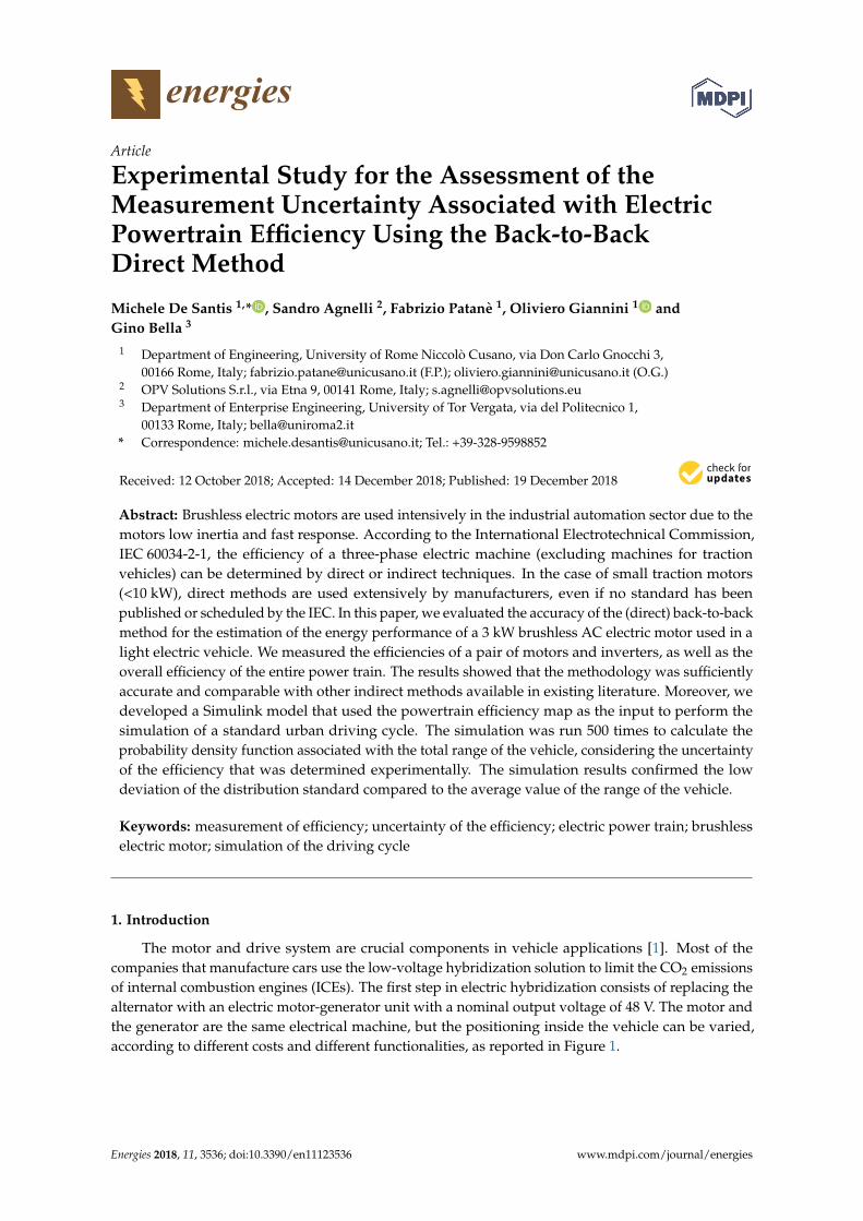
Figure 1. Graphical description of the five hybridization schemes from P0 to P5, considering the different positioning of the electrical machines in the powertrain of the vehicle.

Then, a 48/12 V converter and a small battery storage system are added. A similar system was shown to reduce fuel consumption by as much as 5%, as measured in the New European Driving Cycle (NEDC) [2]. The following steps provide an increasing level of hybridization, up to the fifth hybridization scheme (P5 in Figure 1), which consists of two electric motor-generator units located in the rear wheels. This final architecture of the powertrain allows the vehicle to travel a limited distance in full electric drive. Its performance is based on the continuous power offered by the batteries to maximize the range of the vehicle. Analysis and estimation of the power loss and efficiency of the drivetrain are of practical significance in this matter [3]. As an example, the drive components in the system simulation tools are typically designed based on the efficiency maps of the motor, which is a cost-effective method for optimizing the power consumption and power efficiency over the required ranges of torque and speed [4–7].

Testing of electric machines is regulated by the IEC commission as described in the IEC 60,034 documents, which provide several guidelines, such as IEC 60034-30-2 [8], which is focused on the technical specifications of permanent-magnet, synchronous motors. In particular, the standard considers up to four classes of efficiency, and it groups motors according to their output power and number of poles. Since 1 January 2017, all motors with a rated power between 0.75 and 375 kW are required to comply with the IE3 efficiency, which is premium efficiency in International Efficiency classification [9].

Efficiency, as described in the IEC standards, can be estimated directly or indirectly. A direct measurement is based on the evaluation of input power from voltage and current, and the output power is measured based on the rotational speed and torque. Direct measurement methods are usually considered to be complex, and their implementation is expensive and difficult to perform in terms of the accuracy of the specifications of laboratory instrumentation. Thus, the IEC standards recommend that the efficiency of motors be estimated indirectly, i.e., by measuring the input power and computing the output power by estimating the losses within the motor, as described in the IEC TS 60349-3 documents [10]. IEC 60034-30-2 addresses the standardization of efficiency tests of motors with up to eight poles for industrial purposes, and it cannot be applied to permanent magnet motors for small-vehicle traction, which are characterized by high numbers of poles and variable-speed operation. To date, rigorous estimations of the efficiencies of permanent magnet synchronous motors have not been investigated extensively [11–17], because most studies have been focused on induction motors, which are mostly used in industrial applications.

Figure 1. Graphical description of the five hybridization schemes from P0 to P5, considering thedifferent positioning of the electrical machines in the powertrain of the vehicle.

Then, a 48/12 V converter and a small battery storage system are added. A similar system wasshown to reduce fuel consumption by as much as 5%, as measured in the New European DrivingCycle (NEDC) [2]. The following steps provide an increasing level of hybridization, up to the fifthhybridization scheme (P5 in Figure 1), which consists of two electric motor-generator units located inthe rear wheels. This final architecture of the powertrain allows the vehicle to travel a limited distancein full electric drive. Its performance is based on the continuous power offered by the batteries tomaximize the range of the vehicle. Analysis and estimation of the power loss and efficiency of thedrivetrain are of practical significance in this matter [3]. As an example, the drive components in thesystem simulation tools are typically designed based on the efficiency maps of the motor, which is acost-effective method for optimizing the power consumption and power efficiency over the requiredranges of torque and speed [4–7].

Testing of electric machines is regulated by the IEC commission as described in the IEC 60,034documents, which provide several guidelines, such as IEC 60034-30-2 [8], which is focused on thetechnical specifications of permanent-magnet, synchronous motors. In particular, the standardconsiders up to four classes of efficiency, and it groups motors according to their output powerand number of poles. Since 1 January 2017, all motors with a rated power between 0.75 and 375 kWare required to comply with the IE3 efficiency, which is premium efficiency in International Efficiencyclassification [9].

Efficiency, as described in the IEC standards, can be estimated directly or indirectly. A directmeasurement is based on the evaluation of input power from voltage and current, and the outputpower is measured based on the rotational speed and torque. Direct measurement methods areusually considered to be complex, and their implementation is expensive and difficult to perform interms of the accuracy of the specifications of laboratory instrumentation. Thus, the IEC standardsrecommend that the efficiency of motors be estimated indirectly, i.e., by measuring the input powerand computing the output power by estimating the losses within the motor, as described in the IEC TS60349-3 documents [10]. IEC 60034-30-2 addresses the standardization of efficiency tests of motors withup to eight poles for industrial purposes, and it cannot be applied to permanent magnet motors forsmall-vehicle traction, which are characterized by high numbers of poles and variable-speed operation.To date, rigorous estimations of the efficiencies of permanent magnet synchronous motors have not

Energies 2018, 11, 3536 3 of 19

been investigated extensively [11–17], because most studies have been focused on induction motors,which are mostly used in industrial applications.

The increasing demand for the use of small AC motors has stimulated research related to thedevelopment and enhancement of techniques for the measurement of the motors’ efficiency, and forthe computation of the associated accuracy [18–28], where we provide a short review of the relatedresearch papers. In Reference [9], a comparative analysis of direct and indirect efficiency estimationtechniques was presented for a 3 kW, three-phase induction motor, and it was concluded that thedirect determination of efficiency should be used for all sizes of induction motors. The authorsrecommended the use of the direct method rather than the indirect method for three-phase motorswith power ratings ≤1 kW. In Reference [20], the authors proposed the use of a combination of geneticalgorithms to estimate the efficiency of an induction motor, where the uncertainty for a rated outputpower of 3 kW, was only 0.3%, which was within the acceptable range of accuracy. In Reference [21],the same authors showed that the difference between the measured efficiency (direct method) and theefficiency estimated by the authors’ technique (indirect method) was only 0.25%, for a rated powerof 3 kW. In addition, the inaccuracy of the measured efficiency always was less than 1%, but theinaccuracy of the estimated efficiency always was less than 0.03%. The authors obtained similar resultsin Reference [23], where the difference between the measured and estimated efficiency was 0.4%for a 3 kW rated power. In Reference [27], for an 11-kW rated power induction motor, the RealisticError Estimation (REE) was ±0.24%, which was lower than the Worst Case Estimation (WCE) of themethod recommended by the IEEE 112-B standard for polyphase induction motors. In Reference [28],the accuracy difference for a 3-hp machine, when comparing the measured and estimated efficiencies,was 1.2%. The inaccuracy of the former was ±0.65%, whereas it was ±0.35% for the latter, suggestingthat, for this class of electrical machine, the direct method can be considered to be sufficiently accuratecompared to the estimated method. Other advanced techniques for estimating efficiencies, such as thebacterial foraging algorithm [25], when applied to a 7.5 kW induction motor, resulted in inaccuraciesof 1% or less.

Regarding the specific issue of estimating the efficiencies of light traction motors, the IEC hasyet to publish or schedule a standard, whereas the SAE (Society of Automotive Engineers) recentlydeveloped a document that is focused on measurement repeatability [29]. The direct measurementmethod is used via back-to-back dual motor mounting or by means of electromagnetic friction. Thismethod is particularly fitted for the case of light electric vehicles, because they are always equippedwith two motors that are nominally identical. Even though the method is simple and cost-effective, wewere unable to identify any papers in the literature that focused on the efficiency uncertainty analysis,and that were sufficiently rigorous or detailed for the range of working conditions (speed-torque pair)of the motors. Therefore, the purpose of this paper was to evaluate the back-to-back direct method usedto measure the efficiency of the motor of a small electrical vehicle and the efficiency of the overall drivesystem. Uncertainty maps associated with the back-to-back direct method can be useful in variousapplications, where the estimation by means of the simulation of the range of an electric vehicle is acrucial step, the results of which are needed for the design/optimization of the driving control systemor for the overall energy management policy. Specifically, we performed the following to achieve thatgoal: (i) We applied the direct method on the full power train of a small electrical vehicle (2 × 3 kWbrushless motors plus drivers), (ii) We computed the uncertainty maps associated with the measuredefficiency, and (iii) We estimated the uncertainty associated with the range of the vehicle by simulatinga standard Urban Driving Cycle (UDC) [2] in a Simulink environment.

This paper is organized as follows. After a general description of the powertrain, Section 2describes the experimental setup, the experimental procedure, and the computation of the efficiency ofthe powertrain. Section 3 discusses the results of the measurements of efficiency of the powertrainand the corresponding estimation of the uncertainty, which was compared with other studies in theliterature. Section 4 presents the results of the UDC simulation to determine the uncertainty associatedwith the vehicle’s range. Section 5 presents the conclusion.

Energies 2018, 11, 3536 4 of 19

2. Methods

2.1. General Description

The powertrain was part of an electric, 4-wheel vehicle developed within the European-project,HI-QUAD. The vehicle was equipped with two in-wheel motors in the rear wheels, Figure 2. The tworear wheels were independently controlled through an inverter–motor couple, and they provided amaximum power of 3 kW. Each brushless motor was rated for a peak power of 6 kW at 72 V. For safety,in the case of the L6e vehicle category, the European regulation specifies that the on-board DC voltageshould not exceed 60 V, and that the overall maximum power of the vehicle must be less than 6 kW.The previous limitations restricted the power of each motor to 3 kW, and they restricted the voltagefrom the battery pack located under the seats to 51 V. The forward/regenerative mode could becontrolled independently by sending to each inverter, an appropriate analog torque or speed signalsranging between 0.5 and 4.5 V. The inverters contained the power electronics to convert the DC powerfrom the battery into the AC power necessary to drive the motors according to the driver’s command.Three-phase currents were sent from each inverter to the AC brushless motor. The inverters could alsobe programmed to tune the control parameters of the motor for both the torque and speed modalities.The vehicle’s power source was a 51-V, LiFePO4 battery pack, which was equipped with 32 cellsconsisting of a series of 16 pairs of cells. The battery pack was also used to power the other devices inthe vehicle through a 48–12 V DC/DC converter.

Energies 2018, 11, x FOR PEER REVIEW 4 of 19

2. Methods

2.1. General Description

The powertrain was part of an electric, 4-wheel vehicle developed within the European-project, HI-QUAD. The vehicle was equipped with two in-wheel motors in the rear wheels, Figure 2. The two rear wheels were independently controlled through an inverter–motor couple, and they provided a maximum power of 3 kW. Each brushless motor was rated for a peak power of 6 kW at 72 V. For safety, in the case of the L6e vehicle category, the European regulation specifies that the on-board DC voltage should not exceed 60 V, and that the overall maximum power of the vehicle must be less than 6 kW. The previous limitations restricted the power of each motor to 3 kW, and they restricted the voltage from the battery pack located under the seats to 51 V. The forward/regenerative mode could be controlled independently by sending to each inverter, an appropriate analog torque or speed signals ranging between 0.5 and 4.5 V. The inverters contained the power electronics to convert the DC power from the battery into the AC power necessary to drive the motors according to the driver’s command. Three-phase currents were sent from each inverter to the AC brushless motor. The inverters could also be programmed to tune the control parameters of the motor for both the torque and speed modalities. The vehicle’s power source was a 51-V, LiFePO battery pack, which was equipped with 32 cells consisting of a series of 16 pairs of cells. The battery pack was also used to power the other devices in the vehicle through a 48–12 V DC/DC converter.

Figure 2. Electric motors are the powertrain of the Hi-Quad quadricycle, and they are placed inside the rear wheels. The inverters are inside the metal box behind the two seats, the battery pack is divided into two parts, and they are inside the aluminum packages that are located underneath the seats.

2.2. Experimental Setup

The goal was to implement the direct methodology for evaluating the efficiency of the full powertrain transmission in terms of the conversion of electrical energy to mechanical energy and vice versa (regenerative braking). Using a back-to-back configuration, i.e., using one motor as the electromagnetic brake for the other motor, the methodology allows all of the components of the powertrain to be characterized simultaneously. By determining the torque, speed, voltage, and current measurements from the sensors placed at each power-train level, the efficiency of each component of the power chain could be estimated with an associated uncertainty, which must be computed as a function of the accuracy of the instruments that were used on the test bench.

To perform the tests, the powertrain was unmounted from the vehicle and placed on a fixed frame, as shown in Figure 3. The coupling between the two motors consisted of two elastic joints attached to the two rotors and a torque meter. No bearings were added between the torque transducer and the rotor, so there was no need to take into account any additional mechanical losses.

Figure 2. Electric motors are the powertrain of the Hi-Quad quadricycle, and they are placed inside therear wheels. The inverters are inside the metal box behind the two seats, the battery pack is dividedinto two parts, and they are inside the aluminum packages that are located underneath the seats.

2.2. Experimental Setup

The goal was to implement the direct methodology for evaluating the efficiency of the fullpowertrain transmission in terms of the conversion of electrical energy to mechanical energy andvice versa (regenerative braking). Using a back-to-back configuration, i.e., using one motor as theelectromagnetic brake for the other motor, the methodology allows all of the components of thepowertrain to be characterized simultaneously. By determining the torque, speed, voltage, and currentmeasurements from the sensors placed at each power-train level, the efficiency of each componentof the power chain could be estimated with an associated uncertainty, which must be computed as afunction of the accuracy of the instruments that were used on the test bench.

To perform the tests, the powertrain was unmounted from the vehicle and placed on a fixedframe, as shown in Figure 3. The coupling between the two motors consisted of two elastic jointsattached to the two rotors and a torque meter. No bearings were added between the torque transducer

Energies 2018, 11, 3536 5 of 19

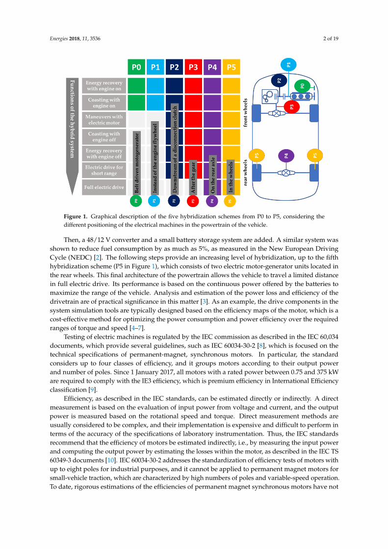
and the rotor, so there was no need to take into account any additional mechanical losses. The twostators were fixed rigidly to the test bench, and misalignments between the joints were reduced toa minimum percentage to cancel possible flexional moments for the torque meter. In the proposedsetup, there was no differential gear since the motors were in-wheel motors, i.e., they were built tobe directly inserted inside the wheels without involving any kind of differential transmission, andthey could be controlled independently. In fact, during the measuring test, one electrical machinewas used as a motor, and the other was used as a brake. Motor 1 and motor 2 were driven by driver1 and driver 2, respectively, which were set in different modalities. Driver 1 was set to speed mode,i.e., the driver tries to keep the rotational speed of the motor as constant as possible, and driver 2was set to torque mode where the driver tries to keep the torque of the motor constant. The supplyvoltages of both driver 1 and driver 2 were kept in the range from 46.4 V to 54.4 V during the tests.Both driver 1 and driver 2 were Sevcon Gen4 36/48 V controllers, whose working voltage ranges aredefined in Table 1. This driver model automatically provides a protection alert when under-voltage orover-voltage threshold limits are exceeded for too much time, and it stops its functioning to avoid theoccurrence of an inverter saturation.

Energies 2018, 11, x FOR PEER REVIEW 5 of 19

The two stators were fixed rigidly to the test bench, and misalignments between the joints were reduced to a minimum percentage to cancel possible flexional moments for the torque meter. In the proposed setup, there was no differential gear since the motors were in-wheel motors, i.e., they were built to be directly inserted inside the wheels without involving any kind of differential transmission, and they could be controlled independently. In fact, during the measuring test, one electrical machine was used as a motor, and the other was used as a brake. Motor 1 and motor 2 were driven by driver 1 and driver 2, respectively, which were set in different modalities. Driver 1 was set to speed mode, i.e., the driver tries to keep the rotational speed of the motor as constant as possible, and driver 2 was set to torque mode where the driver tries to keep the torque of the motor constant. The supply voltages of both driver 1 and driver 2 were kept in the range from 46.4 V to 54.4 V during the tests. Both driver 1 and driver 2 were Sevcon Gen4 36/48 V controllers, whose working voltage ranges are defined in Table 1. This driver model automatically provides a protection alert when under-voltage or over-voltage threshold limits are exceeded for too much time, and it stops its functioning to avoid the occurrence of an inverter saturation.

Figure 3. Bench test for the powertrain.

Figure 3. Bench test for the powertrain.

Energies 2018, 11, 3536 6 of 19

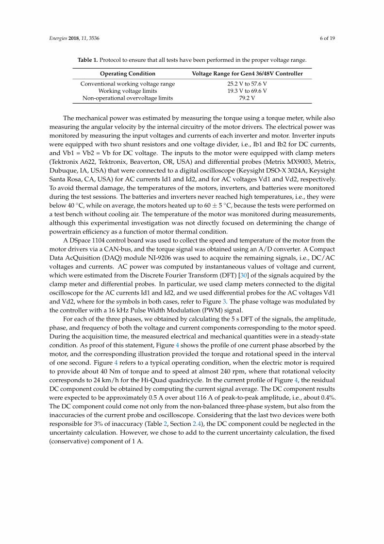
Table 1. Protocol to ensure that all tests have been performed in the proper voltage range.

Operating Condition Voltage Range for Gen4 36/48V Controller

Conventional working voltage range 25.2 V to 57.6 VWorking voltage limits 19.3 V to 69.6 V

Non-operational overvoltage limits 79.2 V

The mechanical power was estimated by measuring the torque using a torque meter, while alsomeasuring the angular velocity by the internal circuitry of the motor drivers. The electrical power wasmonitored by measuring the input voltages and currents of each inverter and motor. Inverter inputswere equipped with two shunt resistors and one voltage divider, i.e., Ib1 and Ib2 for DC currents,and Vb1 = Vb2 = Vb for DC voltage. The inputs to the motor were equipped with clamp meters(Tektronix A622, Tektronix, Beaverton, OR, USA) and differential probes (Metrix MX9003, Metrix,Dubuque, IA, USA) that were connected to a digital oscilloscope (Keysight DSO-X 3024A, KeysightSanta Rosa, CA, USA) for AC currents Id1 and Id2, and for AC voltages Vd1 and Vd2, respectively.To avoid thermal damage, the temperatures of the motors, inverters, and batteries were monitoredduring the test sessions. The batteries and inverters never reached high temperatures, i.e., they werebelow 40 ◦C, while on average, the motors heated up to 60± 5 ◦C, because the tests were performed ona test bench without cooling air. The temperature of the motor was monitored during measurements,although this experimental investigation was not directly focused on determining the change ofpowertrain efficiency as a function of motor thermal condition.

A DSpace 1104 control board was used to collect the speed and temperature of the motor from themotor drivers via a CAN-bus, and the torque signal was obtained using an A/D converter. A CompactData AcQuisition (DAQ) module NI-9206 was used to acquire the remaining signals, i.e., DC/ACvoltages and currents. AC power was computed by instantaneous values of voltage and current,which were estimated from the Discrete Fourier Transform (DFT) [30] of the signals acquired by theclamp meter and differential probes. In particular, we used clamp meters connected to the digitaloscilloscope for the AC currents Id1 and Id2, and we used differential probes for the AC voltages Vd1and Vd2, where for the symbols in both cases, refer to Figure 3. The phase voltage was modulated bythe controller with a 16 kHz Pulse Width Modulation (PWM) signal.

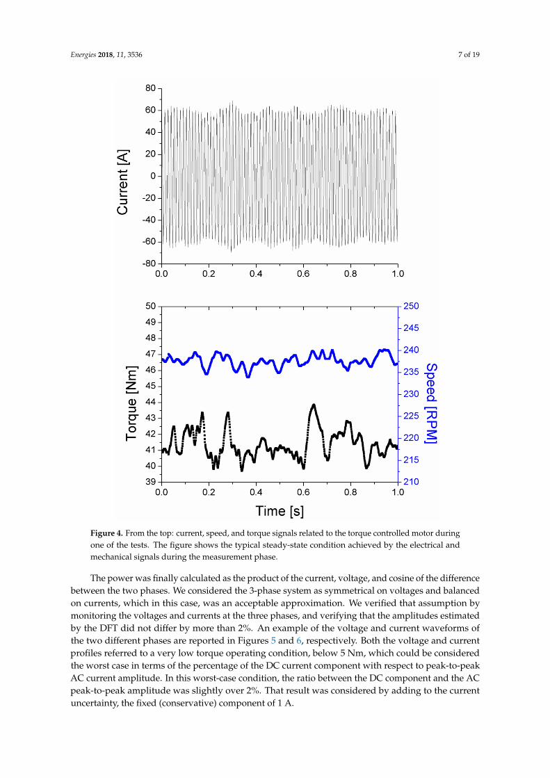
For each of the three phases, we obtained by calculating the 5 s DFT of the signals, the amplitude,phase, and frequency of both the voltage and current components corresponding to the motor speed.During the acquisition time, the measured electrical and mechanical quantities were in a steady-statecondition. As proof of this statement, Figure 4 shows the profile of one current phase absorbed by themotor, and the corresponding illustration provided the torque and rotational speed in the intervalof one second. Figure 4 refers to a typical operating condition, when the electric motor is requiredto provide about 40 Nm of torque and to speed at almost 240 rpm, where that rotational velocitycorresponds to 24 km/h for the Hi-Quad quadricycle. In the current profile of Figure 4, the residualDC component could be obtained by computing the current signal average. The DC component resultswere expected to be approximately 0.5 A over about 116 A of peak-to-peak amplitude, i.e., about 0.4%.The DC component could come not only from the non-balanced three-phase system, but also from theinaccuracies of the current probe and oscilloscope. Considering that the last two devices were bothresponsible for 3% of inaccuracy (Table 2, Section 2.4), the DC component could be neglected in theuncertainty calculation. However, we chose to add to the current uncertainty calculation, the fixed(conservative) component of 1 A.

Energies 2018, 11, 3536 7 of 19Energies 2018, 11, x FOR PEER REVIEW 7 of 19

Figure 4. From the top: current, speed, and torque signals related to the torque controlled motor during one of the tests. The figure shows the typical steady-state condition achieved by the electrical and mechanical signals during the measurement phase.

The power was finally calculated as the product of the current, voltage, and cosine of the difference between the two phases. We considered the 3-phase system as symmetrical on voltages and balanced on currents, which in this case, was an acceptable approximation. We verified that assumption by monitoring the voltages and currents at the three phases, and verifying that the amplitudes estimated by the DFT did not differ by more than 2%. An example of the voltage and current waveforms of the two different phases are reported in Figures 5 and 6, respectively. Both the voltage and current profiles referred to a very low torque operating condition, below 5 Nm, which could be considered the worst case in terms of the percentage of the DC current component with respect to peak-to-peak AC current amplitude. In this worst-case condition, the ratio between the DC component and the AC peak-to-peak amplitude was slightly over 2%. That result was considered by adding to the current uncertainty, the fixed (conservative) component of 1 A.

Figure 4. From the top: current, speed, and torque signals related to the torque controlled motor duringone of the tests. The figure shows the typical steady-state condition achieved by the electrical andmechanical signals during the measurement phase.

The power was finally calculated as the product of the current, voltage, and cosine of the differencebetween the two phases. We considered the 3-phase system as symmetrical on voltages and balancedon currents, which in this case, was an acceptable approximation. We verified that assumption bymonitoring the voltages and currents at the three phases, and verifying that the amplitudes estimatedby the DFT did not differ by more than 2%. An example of the voltage and current waveforms ofthe two different phases are reported in Figures 5 and 6, respectively. Both the voltage and currentprofiles referred to a very low torque operating condition, below 5 Nm, which could be consideredthe worst case in terms of the percentage of the DC current component with respect to peak-to-peakAC current amplitude. In this worst-case condition, the ratio between the DC component and the ACpeak-to-peak amplitude was slightly over 2%. That result was considered by adding to the currentuncertainty, the fixed (conservative) component of 1 A.

Energies 2018, 11, 3536 8 of 19Energies 2018, 11, x FOR PEER REVIEW 8 of 19

Figure 5. Voltage waveforms: the averaged signal and the Discrete Fourier Transform (DFT) signal are reported for each phase. One phase is red and the other one is blue, and the amplitudes are equal to 2% of accuracy, and the voltage profiles are 120° out of phase with the same accuracy.

Figure 6. Current waveforms: one phase is red and the other one is blue. The amplitudes are equal to 2% of accuracy, and the current profiles are 120° out of phase with the same accuracy.

2.3. Experimental Procedure

The efficiency of the powertrain was highly dependent on the current operative condition of the vehicle, and the working range could be wide due to the actual driving scenario and/or the driving style. Therefore, a test bench was used to characterize the performances of the powertrain for the entire ranges over which the torque and rotation speed were varied. In a typical, highly-accurate test bench, the braking torque is controlled and the resulting speed is measured by means of a dedicated electro-magnetic motor. In the case of back-to-back mounting, two nominally-identical motors were tested simultaneously by setting one motor in speed mode and then setting the other motor in torque mode. The experimental procedure consisted of mapping the characteristics of the powertrain conversion by: (i) Setting a target speed on one of the two inverters, (ii) Tuning the target torque on

Figure 5. Voltage waveforms: the averaged signal and the Discrete Fourier Transform (DFT) signal arereported for each phase. One phase is red and the other one is blue, and the amplitudes are equal to 2%of accuracy, and the voltage profiles are 120◦ out of phase with the same accuracy.

Energies 2018, 11, x FOR PEER REVIEW 8 of 19

Figure 5. Voltage waveforms: the averaged signal and the Discrete Fourier Transform (DFT) signal are reported for each phase. One phase is red and the other one is blue, and the amplitudes are equal to 2% of accuracy, and the voltage profiles are 120° out of phase with the same accuracy.

Figure 6. Current waveforms: one phase is red and the other one is blue. The amplitudes are equal to 2% of accuracy, and the current profiles are 120° out of phase with the same accuracy.

2.3. Experimental Procedure

The efficiency of the powertrain was highly dependent on the current operative condition of the vehicle, and the working range could be wide due to the actual driving scenario and/or the driving style. Therefore, a test bench was used to characterize the performances of the powertrain for the entire ranges over which the torque and rotation speed were varied. In a typical, highly-accurate test bench, the braking torque is controlled and the resulting speed is measured by means of a dedicated electro-magnetic motor. In the case of back-to-back mounting, two nominally-identical motors were tested simultaneously by setting one motor in speed mode and then setting the other motor in torque mode. The experimental procedure consisted of mapping the characteristics of the powertrain conversion by: (i) Setting a target speed on one of the two inverters, (ii) Tuning the target torque on

Figure 6. Current waveforms: one phase is red and the other one is blue. The amplitudes are equal to2% of accuracy, and the current profiles are 120◦ out of phase with the same accuracy.

2.3. Experimental Procedure

The efficiency of the powertrain was highly dependent on the current operative condition of thevehicle, and the working range could be wide due to the actual driving scenario and/or the drivingstyle. Therefore, a test bench was used to characterize the performances of the powertrain for theentire ranges over which the torque and rotation speed were varied. In a typical, highly-accuratetest bench, the braking torque is controlled and the resulting speed is measured by means of adedicated electro-magnetic motor. In the case of back-to-back mounting, two nominally-identicalmotors were tested simultaneously by setting one motor in speed mode and then setting the othermotor in torque mode. The experimental procedure consisted of mapping the characteristics of thepowertrain conversion by: (i) Setting a target speed on one of the two inverters, (ii) Tuning the target

Energies 2018, 11, 3536 9 of 19

torque on the other inverter from the minimum to the maximum allowed values, and (iii) Averagingthe sensor data for 5 s, for each value of torque in the stationary condition. The operating status of thepowertrain system during each measurement was in thermal and mechanical steady-state conditions.

Starting from the principle that we were trying to measure the torque characteristics available frommotor 1, we needed motor 2 to function as a brake. The rotational direction of motor 2 was oppositeto that of motor 1, so that motor 2 resisted the rotational motion of motor 1. That came from theback-to-back positioning of the two motors, and in this configuration, the two motors were mirrored,so that if one rotated clockwise, the other rotated counterclockwise to check the speed value of eachmotor (expressed in RPM), and to determine the maximum torque provided by motor 1. Then, motor 1was controlled by driver 1 in the speed mode, but the brake, represented by motor 2, was controlledby driver 2 in the torque mode. This arrangement was chosen for speed control. The three previoussteps were repeated by varying the torque value from the minimum to the maximum allowablevalue, while keeping the speed of motor 1 as constant as possible. This procedure was repeated threetimes for a range of target speeds from 0 to 380 rpm, which allowed us to compute the efficiency ofthe speed-controlled motor–inverter pair (regenerating electrical power), and the torque-controlledmotor–inverter pair.

2.4. Forward and Regenerative Mode Efficiency and Efficiency Uncertainty

This section addresses the estimation of the overall inaccuracies associated with the computationof the efficiency of the powertrain. Nomenclature and propagation rules follow the description inReference [31].

The symbol u(qi) represents the standard uncertainty associated to the measurement of thequantity qi.

The powertrain was equipped with two nominally-identical motors and drivers, operating aselectrical to mechanical (forward mode) and as mechanical to electrical (regenerative mode) energyconverters. Following the scheme reported in Figure 3, four efficiency maps were computed, followingthe nomenclature jηi = Pi/Pj, corresponding to four power conversion operations, i.e., (a) driver 1, bηd;(b) motor 1, dηm; (c) motor 2, mηd; and (d) driver 2, dηb. The forward and regenerative mode efficiencies,i.e., bηm and mηb, corresponded to the generation and regeneration, respectively, of the mechanicalpower, and they could be computed by multiplying, in pairs, the above-mentioned quantities (a, b)and (c, d). The uncertainty associated with the efficiency, jηi, of the generic powertrain componentwas equal to the addition in quadrature of the uncertainties associated with the output and the inputpowers, i.e., Pi and Pj, respectively:

jηi =PiPj⇒ u

(jηi

)= jηi

√1

Pi2 u(Pi)

2 +1

P2j

u(

Pj)2 (1)

The mechanical power, Pm, of a motor can be computed by means of the torque meter output, T,and the velocity of the motor, w, so the associated standard uncertainty of power u(T) is:

Pm = Tω ⇒ u(Pm) = Pm

√1

T2 u(T)2 +1

ω2 u(ω)2 (2)

Regarding the electrical powers, Pb1 and Pb2 and Pd1 and Pd2, that are exchanged between thebattery and the drivers and between the drivers and the motors, respectively:

Pbi = Vb Ibi ⇒ u(Pbi) = Pbi

√1

V2b

u(Vb)2 +

1I2bi

u(Ibi)2 (3)

Pdi = Vd Idi ⇒ u(Pdi) = Pdi

√1

V2di

u(Vdi)2 +

1I2di

u(Idi)2 (4)

Energies 2018, 11, 3536 10 of 19

In Equation (4), the phase error was not considered in the uncertainty calculation.Therefore, taking into account the uncertainties related to the DC/AC voltage and current

measurements, and the uncertainties in the speed and torque measurements of both of the motors,the uncertainty associated with the estimation of the power could be computed for each operatingpoint of the powertrain. Table 2 reports the accuracy budget considered for the computation of theoverall uncertainty.

Table 2. Uncertainty budget for the mechanical and electrical quantities.

Quantity Device Accuracy Distribution

Torque Torque meter ±0.1% reading 2DS1104 ±0.1% reading 2

Speed Inverter ±1 rpm reading√

3

DC voltage and DC current DAQ NI 9206 ±0.1% full scale 2Shunt resistor ±0.25% reading

√3

AC motor currentOscilloscope ±3% reading

√3

Clamp meter ±3% reading ± 50 mA full scale√

3

AC motor voltage Oscilloscope ±3% reading√

3Differential probe ± 2% full scale

√3

3. Results and Discussion

Figure 7 shows the raw data for speed and torque that were collected during the experimentalevaluation of the powertrain. The figure shows that the maximum torque available from the motorwas close to 135 Nm, which was produced at up to 150 rpm. Above 150 rpm, the maximum torquedecreased as the speed increased, following a hyperbolic constant-power trend. Then, it decreasedto zero at the maximum speed of 370 rpm. Note that both of the motors were rated for 220 Nmwhen powered with 72 V, but the reduction of voltage to 51 V caused a corresponding decrease in themaximum available torque to 135 Nm. This behavior was due to the inverter power limitation, whichwas set to 3 kW. The same consideration could be made for the maximum speed value, which neverexceeded 370 rpm, even though the motors were rated for 600 rpm.

Energies 2018, 11, x FOR PEER REVIEW 10 of 19

Therefore, taking into account the uncertainties related to the DC/AC voltage and current measurements, and the uncertainties in the speed and torque measurements of both of the motors, the uncertainty associated with the estimation of the power could be computed for each operating point of the powertrain. Table 2 reports the accuracy budget considered for the computation of the overall uncertainty.

Table 2. Uncertainty budget for the mechanical and electrical quantities.

Quantity Device Accuracy Distribution

Torque Torque meter ±0.1% reading 2 DS1104 ±0.1% reading 2

Speed Inverter ±1 rpm reading √3

DC voltage and DC current DAQ NI 9206 ±0.1% full scale 2 Shunt resistor ±0.25% reading √3

AC motor current Oscilloscope ±3% reading √3

Clamp meter ±3% reading ± 50 mA full scale

√3

AC motor voltage Oscilloscope ±3% reading √3 Differential probe ± 2% full scale √3

3. Results and Discussion

Figure 7 shows the raw data for speed and torque that were collected during the experimental evaluation of the powertrain. The figure shows that the maximum torque available from the motor was close to 135 Nm, which was produced at up to 150 rpm. Above 150 rpm, the maximum torque decreased as the speed increased, following a hyperbolic constant-power trend. Then, it decreased to zero at the maximum speed of 370 rpm. Note that both of the motors were rated for 220 Nm when powered with 72 V, but the reduction of voltage to 51 V caused a corresponding decrease in the maximum available torque to 135 Nm. This behavior was due to the inverter power limitation, which was set to 3 kW. The same consideration could be made for the maximum speed value, which never exceeded 370 rpm, even though the motors were rated for 600 rpm.

Figure 7. Raw speed and torque data gathered by the experimental tests of the powertrain.

The general trend of the experimental data was near-vertical curves. That trend was due to the action of the speed-controlled driver 1. Precisely, Figure 7 shows that the vertical line of blue dots is not properly vertical; rather, it is leaning slightly to the left. This was due to the fact that, as the torque request on driver 2 increased, driver 1 struggled to keep the rotational velocity of motor 1 completely constant. As the torque produced by motor 2 increased, the rotational velocity of motor 1 decreased slightly until the value of the torque provided by motor 2 blocked motor 1. That represented the value of torque that motor 1 was unable to provide to keep its rotational velocity constant. In fact, the

Figure 7. Raw speed and torque data gathered by the experimental tests of the powertrain.

The general trend of the experimental data was near-vertical curves. That trend was due to theaction of the speed-controlled driver 1. Precisely, Figure 7 shows that the vertical line of blue dotsis not properly vertical; rather, it is leaning slightly to the left. This was due to the fact that, as thetorque request on driver 2 increased, driver 1 struggled to keep the rotational velocity of motor 1completely constant. As the torque produced by motor 2 increased, the rotational velocity of motor 1

Energies 2018, 11, 3536 11 of 19

decreased slightly until the value of the torque provided by motor 2 blocked motor 1. That representedthe value of torque that motor 1 was unable to provide to keep its rotational velocity constant. In fact,the capability of maintaining a constant motor speed for driver 1 decreased as the imposed torqueincreased, and that phenomenon was more evident as the speed increased. However, the inaccuracy ofthe speed control at high torque and speed did not affect the estimate of the efficiency, because all ofthe input and output powers were measured constantly. Figure 7 also shows some raw data pointsthat correspond to the preliminary runs of the powertrain, which was tested with two resistive loadsapplied to motor 2. That dynamic braking methodology is called rheostatic braking.

3.1. Power Train Forward-Mode and Regenerative-Mode Efficiencies bηm and mηb

The efficiency map bηm, which corresponds to the torque and speed pairs of Figure 7, is reportedin Figure 8a. The figure shows that, irrespective of the speed of the motor, the powertrain had alow forward mode efficiency for small torques. The same performance was observed for low speeds,i.e., speeds less than 50 rpm, irrespective of the amplitude of the torque. As the speed of the motorincreased, the efficiency of the powertrain increased as the torque request increased. In the speedrange of 50–100 rpm and for values of torque greater than 30 Nm, the efficiency, bηm, was in the rangeof 0.6 to 0.7. In the same range of torque values, a slight increment in speed resulted in a higherefficiency, which approached 0.8 at 150 rpm in the 50–100 Nm range of torque values. The highestpowertrain performance was reached close to the maximum speed, i.e., in the torque range of 60–80 Nm.The maximum efficiency value was 0.88, which indicated that the powertrain that was tested provideda good performance. In terms of efficiency, the results that were obtained showed a battery-to-groundefficiency that was comparable to typical Permanent Magnet Synchronous Motor (PMSM) drivesystems with three-level inverters [14].

Figure 8b shows the total efficiency in regenerative mode, mηb, that was estimated by means ofmotor 2 and driver 2. The map was similar to the map obtained in the forward mode, but in thiscase, the powertrain exhibited an overall higher efficiency. For low values of motor speed, i.e., below100 rpm and above 20 Nm, the powertrain’s regenerative efficiency did not exceed 0.75. The efficiencyreached 0.8 when the speed of the motor was increased to 150 rpm. In the speed range of 150–250 rpmand in the torque range of 20–90 Nm, the efficiency was about 0.88. The best performance was foundwhen the speed ranged from 270–330 rpm and the torque was 15–60 Nm, i.e., mηd reached the value of0.9. In the same area, the forward mode efficiency was 0.88. In the range of low speeds, i.e., 0–15 rpm,the performance of the powertrain was poor, especially as the torque increased. Figure 8b showsthat the powertrain must run at a low speed to achieve a significant regeneration of power. In fact,a minimum of 100 rpm was sufficient to regenerate 60% of the mechanical power.

Energies 2018, 11, x FOR PEER REVIEW 11 of 19

capability of maintaining a constant motor speed for driver 1 decreased as the imposed torque increased, and that phenomenon was more evident as the speed increased. However, the inaccuracy of the speed control at high torque and speed did not affect the estimate of the efficiency, because all of the input and output powers were measured constantly. Figure 7 also shows some raw data points that correspond to the preliminary runs of the powertrain, which was tested with two resistive loads applied to motor 2. That dynamic braking methodology is called rheostatic braking.

3.1. Power Train Forward-Mode and Regenerative-Mode Efficiencies and

The efficiency map , which corresponds to the torque and speed pairs of Figure 7, is reported in Figure 8a. The figure shows that, irrespective of the speed of the motor, the powertrain had a low forward mode efficiency for small torques. The same performance was observed for low speeds, i.e., speeds less than 50 rpm, irrespective of the amplitude of the torque. As the speed of the motor increased, the efficiency of the powertrain increased as the torque request increased. In the speed range of 50–100 rpm and for values of torque greater than 30 Nm, the efficiency, , was in the range of 0.6 to 0.7. In the same range of torque values, a slight increment in speed resulted in a higher efficiency, which approached 0.8 at 150 rpm in the 50–100 Nm range of torque values. The highest powertrain performance was reached close to the maximum speed, i.e., in the torque range of 60–80 Nm. The maximum efficiency value was 0.88, which indicated that the powertrain that was tested provided a good performance. In terms of efficiency, the results that were obtained showed a battery-to-ground efficiency that was comparable to typical Permanent Magnet Synchronous Motor (PMSM) drive systems with three-level inverters [14].

Figure 8b shows the total efficiency in regenerative mode, , that was estimated by means of motor 2 and driver 2. The map was similar to the map obtained in the forward mode, but in this case, the powertrain exhibited an overall higher efficiency. For low values of motor speed, i.e., below 100 rpm and above 20 Nm, the powertrain’s regenerative efficiency did not exceed 0.75. The efficiency reached 0.8 when the speed of the motor was increased to 150 rpm. In the speed range of 150–250 rpm and in the torque range of 20–90 Nm, the efficiency was about 0.88. The best performance was found when the speed ranged from 270–330 rpm and the torque was 15–60 Nm, i.e., reached the value of 0.9. In the same area, the forward mode efficiency was 0.88. In the range of low speeds, i.e., 0–15 rpm, the performance of the powertrain was poor, especially as the torque increased. Figure 8b shows that the powertrain must run at a low speed to achieve a significant regeneration of power. In fact, a minimum of 100 rpm was sufficient to regenerate 60% of the mechanical power.

(a) (b)

Figure 8. Overall efficiency in mechanical power: (a) generation; (b) regeneration.

3.2. Forward-Mode efficiencies of the Motor and Driver and

Figure 9 shows the specific forward efficiencies of motor 1 and driver 1, i.e., and , respectively.

Figure 8. Overall efficiency in mechanical power: (a) generation; (b) regeneration.

Energies 2018, 11, 3536 12 of 19

3.2. Forward-Mode Efficiencies of the Motor and Driver dηm and bηd

Figure 9 shows the specific forward efficiencies of motor 1 and driver 1, i.e., dηm andbηd, respectively.

The forward-mode efficiency of motor 1, dηm, as shown in Figure 9a, increased rapidly up to 0.75,as long as the speed was less than 100 rpm. When the speed was greater than 100 rpm, the efficiencyof the motor increased and reached its maximum values as the speed increased and the torque requestwas in the range of 30–100 Nm. The best performance of the motor was in the torque range of60–80 Nm. As the speed was close to 270 rpm, the efficiency reached the value of 0.92, a result thatwas in accordance with recent studies on the efficiencies of Permanent Magnet (PM) motors [15,16].The highest efficiency was attained when both the driver and the motor maps achieved their bestperformances, i.e., in the speed range of 270–330 Nm and the torque range of 60–80 Nm. The efficiencydecreased rapidly to less than 0.5 when the torque values were less than 20 Nm.

The driver 1 forward-mode efficiency, bηd, shown in Figure 9b, had high values, i.e., greater than0.9, for the torque range of 30–130 Nm, and for speeds greater than 30 rpm. The maximum values weremostly concentrated in the area delimited by speed from 50 to 100 rpm, and by torque values that weregreater than 40 Nm. In this region of the rpm/torque characteristic, the maximum efficiency reached avalue over 0.95. The worst performance occurred when the speed was set at less than 25 rpm, wherethe efficiency decreased to 0.3, irrespective of the torque. The driver’s efficiency was always higherthan the motor’s efficiency. Figure 9b shows that the driver’s efficiency in the area close to 320 rpm wasvery high. However, due to measurement errors that randomly enhanced the driver’s efficiency values,the result was slightly greater than 1. In terms of visualization, we decided to eliminate the driver’sefficiency values that exceeded 1, since it was physically impossible for this scenario to occur. In fact,the driver’s characteristics in that area were reduced for the sake of visualizing the data. Figure 8ashows the efficiency of the entire powertrain, and the measured data were not deleted after theywere acquired.

In conclusion, the experimental tests of the powertrain, concerning the forward-mode evaluationphase, showed that the decrease in the efficiency was not caused by a specific component of thepowertrain. In fact, the low-efficiency regions observed in bηm were found for the same speed/torqueranges in both of the efficiency maps, i.e., bηd and dηm.

Energies 2018, 11, x FOR PEER REVIEW 12 of 19

The forward-mode efficiency of motor 1, , as shown in Figure 9a, increased rapidly up to 0.75, as long as the speed was less than 100 rpm. When the speed was greater than 100 rpm, the efficiency of the motor increased and reached its maximum values as the speed increased and the torque request was in the range of 30–100 Nm. The best performance of the motor was in the torque range of 60–80 Nm. As the speed was close to 270 rpm, the efficiency reached the value of 0.92, a result that was in accordance with recent studies on the efficiencies of Permanent Magnet (PM) motors [15,16]. The highest efficiency was attained when both the driver and the motor maps achieved their best performances, i.e., in the speed range of 270–330 Nm and the torque range of 60–80 Nm. The efficiency decreased rapidly to less than 0.5 when the torque values were less than 20 Nm.

The driver 1 forward-mode efficiency, , shown in Figure 9b, had high values, i.e., greater than 0.9, for the torque range of 30–130 Nm, and for speeds greater than 30 rpm. The maximum values were mostly concentrated in the area delimited by speed from 50 to 100 rpm, and by torque values that were greater than 40 Nm. In this region of the rpm/torque characteristic, the maximum efficiency reached a value over 0.95. The worst performance occurred when the speed was set at less than 25 rpm, where the efficiency decreased to 0.3, irrespective of the torque. The driver’s efficiency was always higher than the motor’s efficiency. Figure 9b shows that the driver’s efficiency in the area close to 320 rpm was very high. However, due to measurement errors that randomly enhanced the driver’s efficiency values, the result was slightly greater than 1. In terms of visualization, we decided to eliminate the driver’s efficiency values that exceeded 1, since it was physically impossible for this scenario to occur. In fact, the driver’s characteristics in that area were reduced for the sake of visualizing the data. Figure 8a shows the efficiency of the entire powertrain, and the measured data were not deleted after they were acquired.

In conclusion, the experimental tests of the powertrain, concerning the forward-mode evaluation phase, showed that the decrease in the efficiency was not caused by a specific component of the powertrain. In fact, the low-efficiency regions observed in were found for the same speed/torque ranges in both of the efficiency maps, i.e., and .

(a) (b)

Figure 9. Efficiency in power generation: (a) motor 1; (b) driver 1.

3.3. Regenerative-Mode Efficiencies of the Motor and Driver and

Figure 10a shows the efficiency of motor 2 in the regenerative mode. The performance of motor 2 resulted in an efficiency map that was similar to that obtained by testing motor 1 in the forward mode. The efficiency was in the range of 0.2 to 0.7 when below 50 rpm, and it was independent of the torque values. For higher speed values, i.e., in the range of 150–300 rpm in the same central torque interval of 30–80 Nm, the efficiency remained high at about 0.9. The peak efficiencies, i.e., near 0.93, occurred in the speed range of 200–270 rpm and the torque range of 30–70 Nm. This region of peak efficiency was clearly visible in the efficiency map of motor 1 for the same speed and torque ranges, and the peak value of efficiency was also very close to that of motor 2. In the last part, i.e., for speeds

Figure 9. Efficiency in power generation: (a) motor 1; (b) driver 1.

3.3. Regenerative-Mode Efficiencies of the Motor and Driver mηd and dηb

Figure 10a shows the efficiency of motor 2 in the regenerative mode. The performance of motor 2resulted in an efficiency map that was similar to that obtained by testing motor 1 in the forward mode.The efficiency was in the range of 0.2 to 0.7 when below 50 rpm, and it was independent of the torquevalues. For higher speed values, i.e., in the range of 150–300 rpm in the same central torque interval of30–80 Nm, the efficiency remained high at about 0.9. The peak efficiencies, i.e., near 0.93, occurred in

Energies 2018, 11, 3536 13 of 19

the speed range of 200–270 rpm and the torque range of 30–70 Nm. This region of peak efficiency wasclearly visible in the efficiency map of motor 1 for the same speed and torque ranges, and the peakvalue of efficiency was also very close to that of motor 2. In the last part, i.e., for speeds greater than350 rpm and for torque in the range of 20–40 Nm, the efficiency was around 0.8. For the same speedrange with the torque less than 20 Nm, the efficiency decreased to 0.2 as the torque decreased.

Figure 10b shows the efficiency map, dηb, of driver 2 in the regenerative mode. The behaviorof driver 2 was similar to that of driver 1 in the forward mode for motor 1 and motor 2. In fact,the regenerative mode condition did not change the driver efficiency significantly, rather it wasindependent of the applied torque, and it remained above 0.8 for motor speeds greater than 50 rpm.For lower speeds and for torque values less than 50 Nm, the efficiency was high, i.e., always greaterthan 0.9, and the same behavior was observed for driver 1 in the forward mode.

Energies 2018, 11, x FOR PEER REVIEW 13 of 19

greater than 350 rpm and for torque in the range of 20–40 Nm, the efficiency was around 0.8. For the same speed range with the torque less than 20 Nm, the efficiency decreased to 0.2 as the torque decreased.

Figure 10b shows the efficiency map, , of driver 2 in the regenerative mode. The behavior of driver 2 was similar to that of driver 1 in the forward mode for motor 1 and motor 2. In fact, the regenerative mode condition did not change the driver efficiency significantly, rather it was independent of the applied torque, and it remained above 0.8 for motor speeds greater than 50 rpm. For lower speeds and for torque values less than 50 Nm, the efficiency was high, i.e., always greater than 0.9, and the same behavior was observed for driver 1 in the forward mode.

(a) (b)

Figure 10. Efficiency in generating power: (a) motor 2; (b) driver 2.

3.4. Efficiency Uncertainty

Using the uncertainty propagation procedure defined in Section 2.4, the overall uncertainty associated with the forward mode efficiency is shown in Figure 11, which reports versus the torque and speed.

Figure 11. Forward mode efficiency (expanded) uncertainty U associated with driver 1 and motor 1.

Figure 10. Efficiency in generating power: (a) motor 2; (b) driver 2.

3.4. Efficiency Uncertainty

Using the uncertainty propagation procedure defined in Section 2.4, the overall uncertaintyassociated with the forward mode efficiency is shown in Figure 11, which reports U

(bηm

)versus the

torque and speed.

Energies 2018, 11, x FOR PEER REVIEW 13 of 19

greater than 350 rpm and for torque in the range of 20–40 Nm, the efficiency was around 0.8. For the same speed range with the torque less than 20 Nm, the efficiency decreased to 0.2 as the torque decreased.

Figure 10b shows the efficiency map, , of driver 2 in the regenerative mode. The behavior of driver 2 was similar to that of driver 1 in the forward mode for motor 1 and motor 2. In fact, the regenerative mode condition did not change the driver efficiency significantly, rather it was independent of the applied torque, and it remained above 0.8 for motor speeds greater than 50 rpm. For lower speeds and for torque values less than 50 Nm, the efficiency was high, i.e., always greater than 0.9, and the same behavior was observed for driver 1 in the forward mode.

(a) (b)

Figure 10. Efficiency in generating power: (a) motor 2; (b) driver 2.

3.4. Efficiency Uncertainty

Using the uncertainty propagation procedure defined in Section 2.4, the overall uncertainty associated with the forward mode efficiency is shown in Figure 11, which reports versus the torque and speed.

Figure 11. Forward mode efficiency (expanded) uncertainty U associated with driver 1 and motor 1.

Figure 11. Forward mode efficiency (expanded) uncertainty U(

bηm

)associated with driver 1 and

motor 1.

Energies 2018, 11, 3536 14 of 19

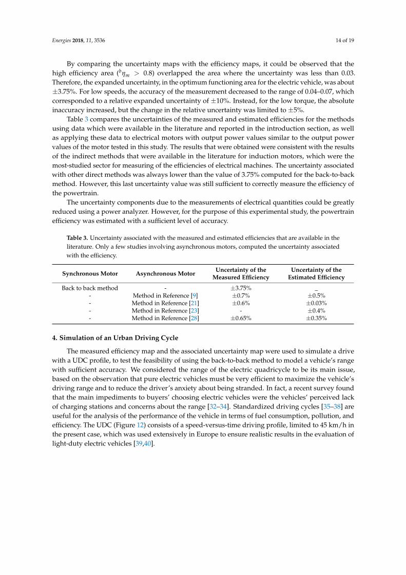
By comparing the uncertainty maps with the efficiency maps, it could be observed that thehigh efficiency area (bηm > 0.8) overlapped the area where the uncertainty was less than 0.03.Therefore, the expanded uncertainty, in the optimum functioning area for the electric vehicle, was about±3.75%. For low speeds, the accuracy of the measurement decreased to the range of 0.04–0.07, whichcorresponded to a relative expanded uncertainty of ±10%. Instead, for the low torque, the absoluteinaccuracy increased, but the change in the relative uncertainty was limited to ±5%.

Table 3 compares the uncertainties of the measured and estimated efficiencies for the methodsusing data which were available in the literature and reported in the introduction section, as wellas applying these data to electrical motors with output power values similar to the output powervalues of the motor tested in this study. The results that were obtained were consistent with the resultsof the indirect methods that were available in the literature for induction motors, which were themost-studied sector for measuring of the efficiencies of electrical machines. The uncertainty associatedwith other direct methods was always lower than the value of 3.75% computed for the back-to-backmethod. However, this last uncertainty value was still sufficient to correctly measure the efficiency ofthe powertrain.

The uncertainty components due to the measurements of electrical quantities could be greatlyreduced using a power analyzer. However, for the purpose of this experimental study, the powertrainefficiency was estimated with a sufficient level of accuracy.

Table 3. Uncertainty associated with the measured and estimated efficiencies that are available in theliterature. Only a few studies involving asynchronous motors, computed the uncertainty associatedwith the efficiency.

Synchronous Motor Asynchronous Motor Uncertainty of theMeasured Efficiency

Uncertainty of theEstimated Efficiency

Back to back method - ±3.75% _- Method in Reference [9] ±0.7% ±0.5%- Method in Reference [21] ±0.6% ±0.03%- Method in Reference [23] - ±0.4%- Method in Reference [28] ±0.65% ±0.35%

4. Simulation of an Urban Driving Cycle

The measured efficiency map and the associated uncertainty map were used to simulate a drivewith a UDC profile, to test the feasibility of using the back-to-back method to model a vehicle’s rangewith sufficient accuracy. We considered the range of the electric quadricycle to be its main issue,based on the observation that pure electric vehicles must be very efficient to maximize the vehicle’sdriving range and to reduce the driver’s anxiety about being stranded. In fact, a recent survey foundthat the main impediments to buyers’ choosing electric vehicles were the vehicles’ perceived lackof charging stations and concerns about the range [32–34]. Standardized driving cycles [35–38] areuseful for the analysis of the performance of the vehicle in terms of fuel consumption, pollution, andefficiency. The UDC (Figure 12) consists of a speed-versus-time driving profile, limited to 45 km/h inthe present case, which was used extensively in Europe to ensure realistic results in the evaluation oflight-duty electric vehicles [39,40].

Energies 2018, 11, 3536 15 of 19Energies 2018, 11, x FOR PEER REVIEW 15 of 19

Figure 12. Urban Driving Cycle (UDC) velocity profile, limited to 45 km/h: the driving cycle consists of three steps of acceleration and deceleration actions.

The UDC simulation was run in the Simulink environment using the efficiency maps to compute the actual power consumption of the torque–speed powertrain. The Simulink model (Figure 13) uses the following electrical/mechanical parameters as inputs, i.e., the battery pack model, electric motor data, maximum torque, reduction ratio, and other mechanical quantities from the motor and from the vehicle chassis (mass, moment of inertia, friction). The motor that was modeled was the standard Simscape servomotor. The battery model considered the discharge curve of a single cell [41] and the nominal and residual capacities.

Figure 13. Block diagram of the UDC simulation: electrical/mechanical quantities reported inside the red boxes were evaluated experimentally.

The electrical capacity of the battery is a function of the time integral of the electrical current absorbed by the powertrain during the execution of the UDC. Each UDC simulation started with the

Figure 12. Urban Driving Cycle (UDC) velocity profile, limited to 45 km/h: the driving cycle consistsof three steps of acceleration and deceleration actions.

The UDC simulation was run in the Simulink environment using the efficiency maps to computethe actual power consumption of the torque–speed powertrain. The Simulink model (Figure 13) usesthe following electrical/mechanical parameters as inputs, i.e., the battery pack model, electric motordata, maximum torque, reduction ratio, and other mechanical quantities from the motor and fromthe vehicle chassis (mass, moment of inertia, friction). The motor that was modeled was the standardSimscape servomotor. The battery model considered the discharge curve of a single cell [41] and thenominal and residual capacities.

Energies 2018, 11, x FOR PEER REVIEW 15 of 19

Figure 12. Urban Driving Cycle (UDC) velocity profile, limited to 45 km/h: the driving cycle consists of three steps of acceleration and deceleration actions.

The UDC simulation was run in the Simulink environment using the efficiency maps to compute the actual power consumption of the torque–speed powertrain. The Simulink model (Figure 13) uses the following electrical/mechanical parameters as inputs, i.e., the battery pack model, electric motor data, maximum torque, reduction ratio, and other mechanical quantities from the motor and from the vehicle chassis (mass, moment of inertia, friction). The motor that was modeled was the standard Simscape servomotor. The battery model considered the discharge curve of a single cell [41] and the nominal and residual capacities.

Figure 13. Block diagram of the UDC simulation: electrical/mechanical quantities reported inside the red boxes were evaluated experimentally.

The electrical capacity of the battery is a function of the time integral of the electrical current absorbed by the powertrain during the execution of the UDC. Each UDC simulation started with the

Figure 13. Block diagram of the UDC simulation: electrical/mechanical quantities reported inside thered boxes were evaluated experimentally.

Energies 2018, 11, 3536 16 of 19

The electrical capacity of the battery is a function of the time integral of the electrical currentabsorbed by the powertrain during the execution of the UDC. Each UDC simulation started with thebattery pack fully charged (state of charge (SOC) = 100%), and the simulation ended when the SOCreached the 0% threshold. We performed 500 UDC simulations, which took about 10 h on a quad-coreIntel Xeon e3-1230v6/3.5 GHz processor with 16 GB of Random Access Memory (RAM).

Concerning the efficiency of the power train, because it was impossible to determine the randomor systematic nature of the sources of errors in the measured uncertainty map, in each UDC run, wedecided to estimate the actual efficiency map by adding an efficiency error to the reference value bηm,where the efficiency error for each ith run was defined as:

bεm,i = pi·√

3u(

bηm

)(5)

where pi is a random variable from a rectangular distribution, limited to the range of −1,1. This meansthat the efficiency map for the ith run was always over-estimated or under-estimated. As mentionedpreviously, we chose such a conservative hypothesis because of the absence of information on thecharacteristics of the error sources.

Figure 14 shows a histogram of the UDC simulations. The results of the estimation of the rangewere about 145,115 m with a 95% uncertainty value of about 450 m, i.e., 0.3%. Such a low uncertaintyvalue was due to the fact that the vehicle, when following the UDC pattern, was always working inthe areas of the efficiency maps, where the associated uncertainty was the lowest, i.e., between 1% and0.1%. That result confirmed that the back-to-back direct method was valid for measuring the efficiencyof the powertrain with a low level of associated uncertainty measurements. The simulation indicatedthat the uncertainty of the efficiency measurement was very low when estimating the range of thevehicle for a standard driving cycle.

Energies 2018, 11, x FOR PEER REVIEW 16 of 19

battery pack fully charged (state of charge (SOC) = 100%), and the simulation ended when the SOC reached the 0% threshold. We performed 500 UDC simulations, which took about 10 h on a quad-core Intel Xeon e3-1230v6/3.5 GHz processor with 16 GB of Random Access Memory (RAM).

Concerning the efficiency of the power train, because it was impossible to determine the random or systematic nature of the sources of errors in the measured uncertainty map, in each UDC run, we decided to estimate the actual efficiency map by adding an efficiency error to the reference value , where the efficiency error for each ith run was defined as:

, = ∙ √3 (5)

where pi is a random variable from a rectangular distribution, limited to the range of −1,1. This means that the efficiency map for the ith run was always over-estimated or under-estimated. As mentioned previously, we chose such a conservative hypothesis because of the absence of information on the characteristics of the error sources.

Figure 14 shows a histogram of the UDC simulations. The results of the estimation of the range were about 145,115 m with a 95% uncertainty value of about 450 m, i.e., 0.3%. Such a low uncertainty value was due to the fact that the vehicle, when following the UDC pattern, was always working in the areas of the efficiency maps, where the associated uncertainty was the lowest, i.e., between 1% and 0.1%. That result confirmed that the back-to-back direct method was valid for measuring the efficiency of the powertrain with a low level of associated uncertainty measurements. The simulation indicated that the uncertainty of the efficiency measurement was very low when estimating the range of the vehicle for a standard driving cycle.

Figure 14. Histogram of the vehicle range from the UDC simulation.

5. Conclusions

We evaluated the efficiency and the associated accuracy of the power train of a light electric vehicle to verify the feasibility of the back-to-back direct method. The inaccuracy of the direct method was greater than the inaccuracies of other methods available in the literature, but the values were still comparable. Our results can also be extended to small motors for traction vehicles, when limited to the back-to-back technique. The results reported in another study [9] indicated that the direct methods for electric motors with rated power values greater than 1-kW could be used for all three-phase motors with a sufficient level of accuracy. The performed UDC simulation led to the conclusion that the back-to-back direct method allowed us to obtain accurate information about the overall range of the vehicle when travelling on a standard driving cycle. We could have obtained a lower

Figure 14. Histogram of the vehicle range from the UDC simulation.

5. Conclusions

We evaluated the efficiency and the associated accuracy of the power train of a light electricvehicle to verify the feasibility of the back-to-back direct method. The inaccuracy of the direct methodwas greater than the inaccuracies of other methods available in the literature, but the values were stillcomparable. Our results can also be extended to small motors for traction vehicles, when limited tothe back-to-back technique. The results reported in another study [9] indicated that the direct methods

Energies 2018, 11, 3536 17 of 19

for electric motors with rated power values greater than 1-kW could be used for all three-phase motorswith a sufficient level of accuracy. The performed UDC simulation led to the conclusion that theback-to-back direct method allowed us to obtain accurate information about the overall range of thevehicle when travelling on a standard driving cycle. We could have obtained a lower inaccuracy ofmeasurements using a power analyzer instead of a digital oscilloscope; however, both the powertrainefficiency and the vehicle range were estimated with sufficient accuracy.

No previous research has been conducted on the uncertainty of the measurements associated withthe efficiency of the powertrain using the back-to-back direct method. All uncertainty assessments inthis field have been performed on the asynchronous electric motors used in industries, and most ofthem were conducted using the indirect method. The efficiency of synchronous electric motors usedfor electric vehicles is currently not regulated by standards, but considering the increasing requestsfor electric vehicles in the automotive market, it is likely that this aspect will be investigated in thenear future.

Forthcoming developments of this experimental study concern the improvement of themeasurement uncertainty associated with the electric powertrain efficiency using the back-to-backdirect method, and the estimate of the vehicle’s range to real a UDC and not just to a standard UDC.Furthermore, the experimental estimate of the powertrain efficiency, using the back-to-back directmethod, will be extended to two different useful scenarios: Powertrain efficiency evaluation as afunction of both motor and battery temperatures and powertrain efficiency evaluation as a functionof the state of charge (SoC) of the battery pack. This information could be very useful for on-boardimplementation of a real-time estimation of a vehicle’s effective range.

Author Contributions: Conceptualization, M.D.S. and S.A.; methodology, F.P.; software, S.A., and M.D.S.;validation, M.D.S., S.A., and F.P.; formal analysis, M.D.S., S.A., and O.G.; investigation, S.A., M.D.S., and F.P.;resources, G.B.; data curation, M.D.S., and S.A.; writing—original draft preparation, M.D.S.; writing—review andediting, M.D.S., F.P., and O.G.; visualization, M.D.S., S.A., F.P.; supervision, O.G., and G.B.; project administration,M.D.S., O.G., and G.B.; funding acquisition, G.B.

Funding: This research was funded by the Ministry of Economic Development of Italy, Innovation Industryproject “sustainable mobility” No. MS01_00038.

Acknowledgments: The present research was financed by the Ministry of Economic Development of Italy in thecontest of the project named HI-QUAD.

Conflicts of Interest: The authors declare no conflict of interest.

References

1. Sun, L.; Chan, C.C.; Liang, R.; Wang, Q. State-of-art of Energy System for New Energy Vehicles. In Proceedingsof the IEEE Vehicle Power and Propulsion Conference (VPPC), Harbin, China, 3–5 September 2008. [CrossRef]

2. Barlow, T.J.; Latham, S.; McCrae, I.S.; Boulter, P.G. A Reference Book of Driving Cycles for Use in theMeasurement of Road Vehicle Emissions, TRL Published Project Report 354. 2009. Available online:http://worldcat.org/isbn/9781846088162 (accessed on 25 Juanary 2010).

3. Zhang, C.; Guo, Q.; Li, L.; Wang, M.; Wang, T. System Efficiency Improvement for Electric Vehicles Adoptinga Permanent Magnet Synchronous Motor Direct Drive System. Energies 2017, 10, 2030. [CrossRef]

4. Wang, X.; Wang, S.; Chen, M.; Zhao, H. Efficiency Testing Technology and Evaluation of the ElectricVehicle Motor Drive System. In Proceedings of the IEEE Conference and Expo Transportation ElectrificationAsia-Pacific (ITEC Asia-Pacific), Beijing, China, 31 August–3 September 2014; pp. 1–5.

5. Chen, C.; Mohr, M.; Diwoky, F. Modeling of the System Level Electric Drive Using Efficiency Maps Obtainedby Simulation Methods. In Proceedings of the SAE 2014 World Congress & Exhibition, Detroit, MI, USA,8–10 April 2014. [CrossRef]

6. Oh, S.C. Evaluation of motor characteristics for hybrid electric vehicles using the hardware-in-the-loopconcept. IEEE Trans. Veh. Technol. 2005, 54, 817–824. [CrossRef]

7. Guo, Q.; Zhang, C.; Li, L.; Zhang, J.; Wang, M. Maximum Efficiency per Torque Control of Permanent-MagnetSynchronous Machines. Appl. Sci. 2016, 6, 425. [CrossRef]

Energies 2018, 11, 3536 18 of 19

8. IEC TS 60034-30-2:2016, Rotating Electrical Machines—Part 30-2: Efficiency Classes of Variable SpeedAC Motors (IE-code). 2016. Available online: https://webstore.iec.ch/publication/30830 (accessed on8 December 2016).

9. Bucci, G.; Ciancetta, F.; Fiorucci, E.; Ometto, A. Uncertainty issues in direct and indirect efficiencydetermination for three-phase induction motors: Remarks about the IEC 60034-2-1 Standard. IEEE Trans.Instrum. Meas. 2016, 65, 2701–2716. [CrossRef]

10. IEC TS 60349-3:2010, Electric Traction—Rotating Electrical Machines for Rail and Road Vehicles—Part3: Determination of the Total Losses of Converter-Fed Alternating Current Motors by Summation ofthe Component Losses. 2010. Available online: https://webstore.iec.ch/publication/1830 (accessed on25 March 2010).

11. Ozturk, S.B.; Toliyat, H.A. Direct torque and indirect flux control of brushless DC motor. IEEE/ASMETrans. Mechatron. 2011, 16, 351–360. [CrossRef]

12. Tinazzi, F.; Zigliotto, M. Torque estimation in high-efficiency IPM synchronous motor drives. IEEE Trans.Energy Convers. 2015, 30, 983–990. [CrossRef]

13. Debruyne, C.; Sergeant, P.; Derammelaere, S.; Desmet, J.J.M.; Vandevelde, L. Influence of Supply VoltageDistortion on the Energy Efficiency of Line-Start Permanent-Magnet Motors. IEEE Trans. Ind. Appl. 2014, 50,1034–1043. [CrossRef]

14. Bianchi, N.; Bottesi, O.; Alberti, L. Energy Efficiency Improvement Adopting Synchronous Motors.In Proceedings of the Eighth International Conference and Exhibition on Ecological Vehicles and RenewableEnergies (EVER), Monte Carlo, Monaco, 27–30 March 2013; pp. 1–7. [CrossRef]

15. Sato, D.; Itoh, J. Evaluation method of energy consumption for permanent magnet synchronous motor drivesystem. In Proceedings of the IECON 2015—41st Annual Conference of the IEEE Industrial ElectronicsSociety, Yokohama, Japan, 9–12 November 2015; pp. 005267–005272. [CrossRef]

16. Du, J.; Wang, X.; Lv, H. Optimization of magnet shape based on efficiency map of IPMSM for Evs. IEEE Trans.Appl. Supercond. 2016, 26, 1–7. [CrossRef]

17. Galioto, S.J.; Reddy, P.B.; EL-Rafaie, A.M.; Alexander, J.P. Effect of magnet types on performance of high-speedspoke Interior-Permanent-Magnet machines designed for traction applications. IEEE Trans. Ind. Appl. 2015,51, 2148–2160. [CrossRef]

18. Lu, B.; Habetler, T.G.; Harley, R.G. A survey of efficiency-estimation methods for in-service induction motors.IEEE Trans. Ind. Appl. 2006, 42, 924–933. [CrossRef]

19. Lu, B.; Habetler, T.G.; Harley, R.G. A nonintrusive and in-service motor-efficiency estimation method usingair-gap torque with considerations of condition monitoring. IEEE Trans. Ind. Appl. 2008, 44, 1666–1674.[CrossRef]

20. Al-Badri, M.; Pillay, P.; Angers, P. A Novel in situ efficiency estimation algorithm for three-phase IM usingGA, IEEE method F1 calculations, and pretested motor data. IEEE Trans. Energy Convers. 2015, 30, 1092–1102.[CrossRef]

21. Al-Badri, M.; Pillay, P.; Angers, P. A Novel Algorithm for Estimating Refurbished Three-Phase InductionMotors Efficiency Using Only No-Load Tests. IEEE Trans. Energy Convers. 2015, 30, 615–625. [CrossRef]

22. Verucchi, C.; Ruschetti, C.; Benger, F. Efficiency measurements in induction motors: Comparison of standards.IEEE Latin Am. Trans. 2015, 13, 2602–2607. [CrossRef]

23. Al-Badri, M.; Pillay, P.; Angers, P. A novel technique for in situ efficiency estimation of three-phase IMoperating with unbalanced voltages. IEEE Trans. Ind. Appl. 2016, 52, 2843–2855. [CrossRef]

24. Siraki, A.G.; Gajjar, C.; Khan, M.A.; Barendse, P.; Pillay, P. An algorithm for nonintrusive in situ efficiencyestimation of induction machines operating with unbalanced supply conditions. IEEE Trans. Ind. Appl. 2012,48, 1890–1900. [CrossRef]

25. Sousa Santos, V.; Viego Felipe, P.; Gómez Sarduy, J. Bacterial foraging algorithm application for inductionmotor field efficiency estimation under unbalanced voltages. Measurement 2013, 46, 2232–2237. [CrossRef]

26. Sakthivel, V.P.; Bhuvaneswari, R.; Subramanian, S. An accurate and economical approach for induction motorfield efficiency estimation using bacterial foraging algorithm. Measurement 2011, 44, 674–684. [CrossRef]

27. Gajjar, C.S.; Kinyua, J.M.; Khan, M.A.; Barendse, P.S. Analysis of a nonintrusive efficiency estimationtechnique for induction machines compared to the IEEE 112B and IEC 34-2-1 standards. IEEE Trans.Ind. Appl. 2015, 51, 4541–4553. [CrossRef]

Energies 2018, 11, 3536 19 of 19

28. Siraki, A.; Pillay, P. An in-situ efficiency estimation technique for induction machines working withunbalanced supplies. IEEE Trans. Energy Convers. 2012, 27, 85–95. [CrossRef]

29. SAE J2907, Performance Characterization of Electrified Powertrain Motor-Drive Subsystem. 2018. Availableonline: https://www.sae.org/standards/content/j2907_201802/ (accessed on 12 February 2018).

30. Krajewski, M. Constructing an uncertainty budget for voltage RMS measurement with a sampling voltmeter.Metrologia 2018, 55, 95–105. [CrossRef]

31. Evaluation of Measurement Data—Guide to the Expression of Uncertainty in Measurement, JCGM100:2008, (GUM 1995 with Minor Corrections). Available online: https://www.iso.org/standard/50461.html(accessed on 20 November 2010).

32. Bonges, H.A., III; Lusk, A.C. Addressing electric vehicle (EV) sales and range anxiety through parking layout,policy and regulation. Transp. Res. Part A 2016, 83, 63–73. [CrossRef]

33. Kim, S.; Lee, J.; Lee, C. Does Driving Range of Electric Vehicles Influence Electric Vehicle Adoption?Sustainability 2017, 9, 1783. [CrossRef]

34. Vidhi, R.; Shrivastava, P. A Review of Electric Vehicle Lifecycle Emissions and Policy Recommendations toIncrease EV Penetration in India. Energies 2018, 11, 483. [CrossRef]

35. Ko, J.; Jin, D.; Jang, W.; Myung, C.; Kwon, S.; Park, S. Comparative investigation of NOx emissioncharacteristics from a Euro 6-compliant diesel passenger car over the NEDC and WLTC at various ambienttemperatures. Appl. Energy 2017, 187, 652–662. [CrossRef]

36. Tsiakmakis, S.; Fontaras, G.; Ciuffo, B.; Samaras, Z. A simulation-based methodology for quantifyingeuropean passenger car fleet CO2 emissions. Appl. Energy 2017, 199, 447–465. [CrossRef]

37. Tsokolis, D.; Tsiakmakis, S.; Dimaratos, A.; Fontaras, G.; Pistikopoulos, P.; Ciuffo, B.; Samaras, Z. Fuelconsumption and CO2 emissions of passenger cars over the new worldwide harmonized test protocol.Appl. Energy 2016, 179, 1152–1165. [CrossRef]

38. Wang, H.; Zhang, W.; Ouyang, M. Energy consumption of electric vehicles based on real-world drivingpatterns: A case study of Beijing. Appl. Energy 2015, 157, 710–719. [CrossRef]

39. Chen, L.; Wang, J.; Lazari, P.; Chen, X. Optimizations of a permanent magnet machine targeting differentdriving cycles for electric vehicles. In Proceedings of the IEEE International Electric Machines & DrivesConference (IEMDC), Chicago, IL, USA, 12–15 May 2013; pp. 855–862. [CrossRef]

40. Tranchoa, E.; Ibarra, E.; Arias, A.; Kortabarria, I.; Prieto, P.; Martínez de Alegría, I.; Andreu, J.; López, I.Sensorless control strategy for light-duty EVs and efficiency loss evaluation of high frequency injectionunder standardized urban driving cycles. Appl. Energy 2018, 224, 647–658. [CrossRef]

41. De Santis, M.; Agnelli, S.; Silvestri, L.; Di Ilio, G.; Giannini, O. Characterization of the powertrain componentsfor a hybrid quadricycle. In Proceedings of the international conference of numerical analysis and appliedmathematics 2015 (ICNAAM 2015), Rhodi, Greece, 22–28 September 2015. [CrossRef]

© 2018 by the authors. Licensee MDPI, Basel, Switzerland. This article is an open accessarticle distributed under the terms and conditions of the Creative Commons Attribution(CC BY) license (http://creativecommons.org/licenses/by/4.0/).