Experimental Study of the Effects of Tilt, Shading, and Temperature

on Photovoltaic Panel Performance

Presented to the

University of California, San Diego

Department of Mechanical and Aerospace Engineering

MAE 126A

Date: 2/6/2014

Prepared by:

Section A08 (Friday 1-4pm)

Akash Gupta, Alex Lin, Colin Moynihan, Mei Tsuruta

2

Abstract

Solar energy is one of the most popular and sustainable forms of alternative energy in the

modern age. This experiment explores the effect of various environmental factors on the power

output of two photovoltaic solar panels. The experiments test the effects of power output and

panel efficiency with respect to tilt angle, shading, and temperature. The maximum power output

of 9.96 W was found to occur when the tilt angle is 60°. This was found by testing the response

of the solar panels at various angles. This occurs at the point of maximum irradiance, which

correlates to a higher output. The effect of shading was observed by covering the photovoltaic

panels horizontally and vertically with a completely opaque material. Horizontal shading has a

larger effect than vertical shading on the PV panels due to the wiring of the panel. Finally,

temperature was observed to decrease the electrical conversion efficiency of the panel as

temperature increased.

3

Table of Contents

Abstract ……………………………………………………...……….………………………….. 2

List of Figures ……………………………………………….....……………………………....... 4

Introduction …………………………………………………….....……………………………... 5

Theory …………………………………………………………………………………………… 6

Experimental Procedure …………………………………...…………………………………….. 8

Results ………………………………………………………………………………………..… 11

Discussion (with Error Analysis) …………………………………...………………………….. 20

Conclusion ……………………………………………………………………………………... 23

References …………………………………………...…………………………………………. 24

Appendix ……………………………………………….………………………………………. 25

4

List of Figures

Figure 1. Solar Angles

Figure 2. Effect of Temperature on I-V Curve

Figure 3. Schematics of Solar Panel I-V Measurement System

Figure 4. Connection Diagram for Solar Operational Interface

Figure 5. Panel Shading Coordinates

Figure 6. I-V curves for Kyocera and UniSolar Panels at 0º and 30º

Figure 7. Isc vs Panel Angle of Tilt

Figure 8. Voc vs Panel Angle of Tilt

Figure 9. Least Squares Fit of Vmpp vs Irradiance

Figure 10. Least Squares Fit of Pmpp vs Irradiance

Figure 11. Output Power vs Voltage for Vertical Shading of UniSolar Panel

Figure 12. Output Power vs Voltage for Horizontal Shading of UniSolar Panel

Figure 13. Ratio of Shaded/Unshaded Pmpp vs Ratio of Shaded Area/Total Panel Area

Figure 14. Conversion Efficiency vs Ratio of Shaded Area/Total Panel Area

Figure 15. Pmpp vs Panel Temperature

Figure 16. Electrical Conversion Efficiency vs Panel Temperature

Figure 17. Vmpp vs Panel Temperature

Figure 18. Impp vs Panel Temperature

Figure 19. Corrected Impp vs Panel Temperature

Figure 20. Corrected Electrical Conversion Efficiency vs Panel Temperature

5

Introduction

Devices powered by solar cells are expected to operate under maximum power. To

accomplish this, maximum power point trackers have been used to find a point at which cells

generate maximum power as a product of current and voltage regarding a particular value of

resistance. Specifically, the performance of solar cells is determined by several external factors

such as the angle of incidence of incoming light, shading of the panel, and changes in solar cell

temperature. In this experiment, an EKO MP-170 PV Module & Array Tester is utilized to

compare the performance of two different PV panels as well as investigate the effect of panel tilt,

shading, and cooling on panel performance. Additionally, the reduction in panel power output

and efficiency as a function of shaded panel area and temperature will be measured.

6

Theory

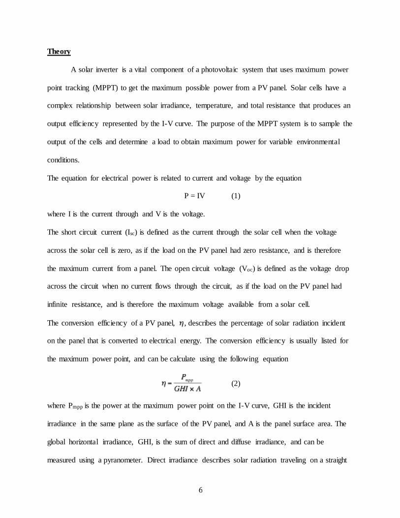
A solar inverter is a vital component of a photovoltaic system that uses maximum power

point tracking (MPPT) to get the maximum possible power from a PV panel. Solar cells have a

complex relationship between solar irradiance, temperature, and total resistance that produces an

output efficiency represented by the I-V curve. The purpose of the MPPT system is to sample the

output of the cells and determine a load to obtain maximum power for variable environmental

conditions.

The equation for electrical power is related to current and voltage by the equation

P = IV (1)

where I is the current through and V is the voltage.

The short circuit current (Isc) is defined as the current through the solar cell when the voltage

across the solar cell is zero, as if the load on the PV panel had zero resistance, and is therefore

the maximum current from a panel. The open circuit voltage (Voc) is defined as the voltage drop

across the circuit when no current flows through the circuit, as if the load on the PV panel had

infinite resistance, and is therefore the maximum voltage available from a solar cell.

The conversion efficiency of a PV panel, , describes the percentage of solar radiation incident

on the panel that is converted to electrical energy. The conversion efficiency is usually listed for

the maximum power point, and can be calculate using the following equation

(2)

where Pmpp is the power at the maximum power point on the I-V curve, GHI is the incident

irradiance in the same plane as the surface of the PV panel, and A is the panel surface area. The

global horizontal irradiance, GHI, is the sum of direct and diffuse irradiance, and can be

measured using a pyranometer. Direct irradiance describes solar radiation traveling on a straight

7

line from the sun to the surface of the panel, while diffuse irradiance describes sunlight that has

been scattered by particles in the atmosphere and comes into contact with the panel.

Figure 1. Solar Angles1 Figure 2. Effect of Temperature on I-V Curve2

When setting up the experiments, the PV panel under measurement is always set up so that the

panel and pyranometer, or sensor unit, are on the same plane relative to the sun, which is

commonly referred to as the “plane of array”. This is a fundamental step in measuring PV

performance, and Fig. 1 shows how to accurately position panels.

Like all other semiconductor devices, solar cells are sensitive to changes in temperature. Fig. 2

shows that an increase in temperature increases Isc slightly and lowers Voc more significantly.

Higher temperatures should then result in a lower maximum power output.

The following formula is used to compute corrected Impp:

)(}{}{ n

measured

n

mppcorrected

n

mpp GHIGHIII (3)

where is the GHI averaged over all measurements, n is the measurement index, and is the

Impp/GHI coefficient. is defined as

GHI

I mpp

(4)

From Eq. (3), corrected Pmpp can be found using the following:

8

measuredmppcorrectedmppcorrectedmpp VIP }{}{}{ (5)

Experimental Procedure

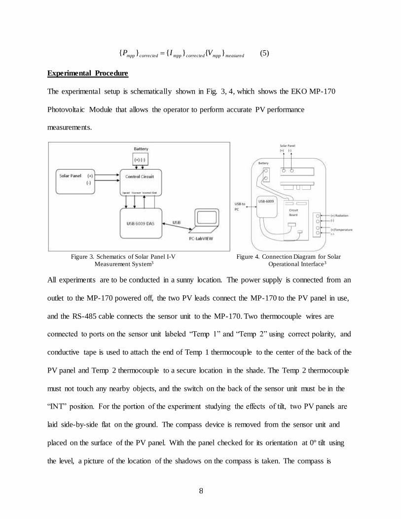
The experimental setup is schematically shown in Fig. 3, 4, which shows the EKO MP-170

Photovoltaic Module that allows the operator to perform accurate PV performance

measurements.

Figure 3. Schematics of Solar Panel I-V Figure 4. Connection Diagram for Solar

Measurement System3 Operational Interface3

All experiments are to be conducted in a sunny location. The power supply is connected from an

outlet to the MP-170 powered off, the two PV leads connect the MP-170 to the PV panel in use,

and the RS-485 cable connects the sensor unit to the MP-170. Two thermocouple wires are

connected to ports on the sensor unit labeled “Temp 1” and “Temp 2” using correct polarity, and

conductive tape is used to attach the end of Temp 1 thermocouple to the center of the back of the

PV panel and Temp 2 thermocouple to a secure location in the shade. The Temp 2 thermocouple

must not touch any nearby objects, and the switch on the back of the sensor unit must be in the

“INT” position. For the portion of the experiment studying the effects of tilt, two PV panels are

laid side-by-side flat on the ground. The compass device is removed from the sensor unit and

placed on the surface of the PV panel. With the panel checked for its orientation at 0º tilt using

the level, a picture of the location of the shadows on the compass is taken. The compass is

9

reattached to the sensor unit, which is aligned so the shadows on the compass match that of the

picture taken. This is done so that the PV panels and pyranometer are on the same plane relative

to the sun.

To take measurements, the sensor unit is powered on, then the MP-170. At the home

screen of the MP-170, press “CONFIG”>highlight “MEAS PAR”>press “Enter”>highlight

“SELECT”>press “Enter”. Highlight the measurement protocol from the “PARAMETER LIST”

that corresponds to the brand of PV panel being used (UniSolar or Kyocera)>press “Enter”. At

the home screen press “MEASURE”. All data are saved after each measurement, and can be

viewed by pressing “DATA”>highlight “SEARCH”>press “Enter”.

For the tilt experiment, measurements are taken for the two PV panels at 0º and 30º tilt.

Only one PV panel can be measured at a time, and the parameters must be changed prior to using

a different panel. Measurements are taken for one PV panel at 10º, 20º, 40º, 50º, and 60º.

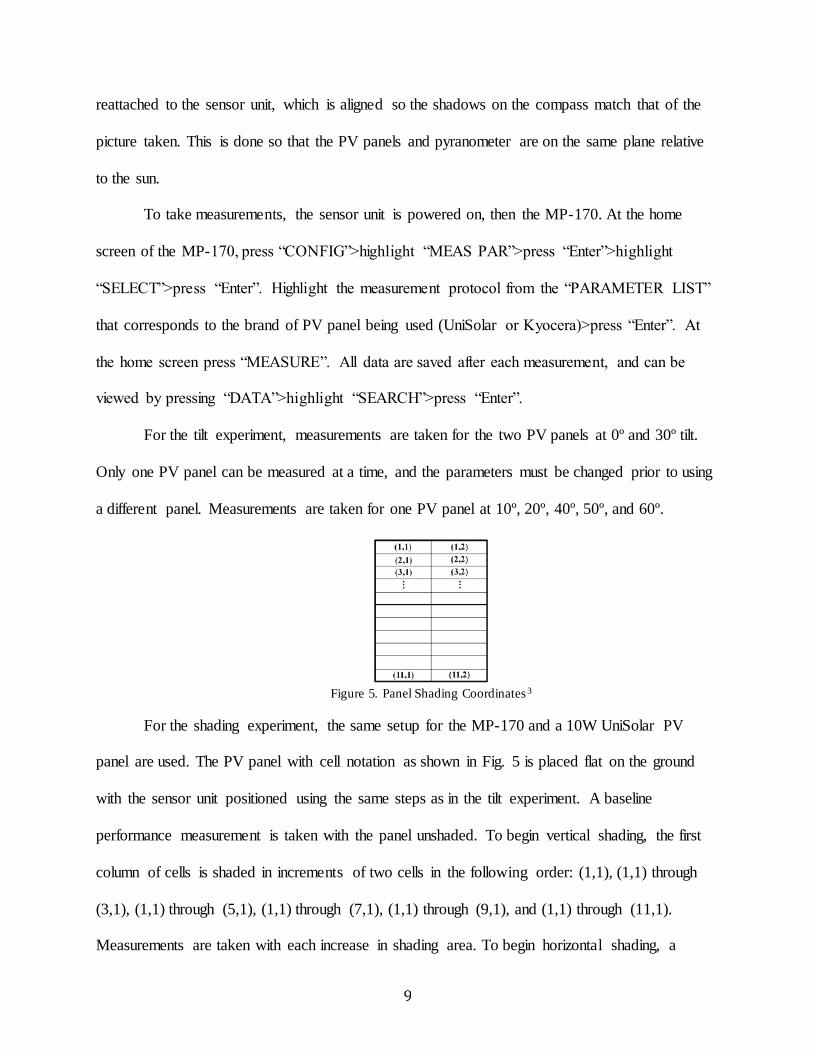
Figure 5. Panel Shading Coordinates3

For the shading experiment, the same setup for the MP-170 and a 10W UniSolar PV

panel are used. The PV panel with cell notation as shown in Fig. 5 is placed flat on the ground

with the sensor unit positioned using the same steps as in the tilt experiment. A baseline

performance measurement is taken with the panel unshaded. To begin vertical shading, the first

column of cells is shaded in increments of two cells in the following order: (1,1), (1,1) through

(3,1), (1,1) through (5,1), (1,1) through (7,1), (1,1) through (9,1), and (1,1) through (11,1).

Measurements are taken with each increase in shading area. To begin horizontal shading, a

10

completely opaque material covers the cells in the following order: Row 1, Rows 1 through 2,

Rows 1 through 3, Rows 1 through 4, and Rows 1 through 5. Measurements are taken with each

increase in shading area.

For the temperature experiment, the same setup for the MP-170 and 10W UniSolar PV

panel are used. One measurement is taken to ensure everything is set up correctly. A plastic bag

is filled with enough ice to cover the entire surface area of the PV panel and placed on the panel

to allow it to cool for 10-15 minutes. The bag is removed and measurements are taken with the

MP-170. Measurements are taken as frequently as possible until the panel reaches a steady state

temperature. Once the panel has reached steady state, 5-10 minutes must pass before repeating

the process with the ice bag and measurements. There should be two complete sets of

measurements.

To download the collected data, access a computer that has the MP-170 Control Program

and USB-COM drivers installed. Connect the MP-170 to the computer using the USB-MiniUSB

cable and turn on the MP-170 if not already powered on. Open the “MP-170 Control Program”

(Start>All Programs> EKO). On the “Measure” tab click “General”. Check that the correct COM

port is selected and the “Data Folder” and “Converted Data Folder” fields show the correct path

for saved files. Click “Ok”. On the “Measure” tab click “Load Data”. All data are saved on the

computer as MDF files, which must be converted. This is done by going to the “Save” tab and

checking that the directory in the field “File Name” is the same as the location of the MDF files.

Select all data records needed by confirming that the “Date” fields shows the same date and time

as the filename of the MDF files and click “Convert”. This generates a CSV file that can be read

using MATLAB or MS Excel.

11

Experimental Results

Week 1: Effects of Tilt on PV Panel Performance

Figure 6. I-V curves for Kyocera and UniSolar Panels at 0º and 30º

The relationship between power and tilt angle can be determined from Fig. 6 by plotting voltage

against current. The power output for both the UniSolar and Kyocera panels is greater when the

tilt angle is at 30º compared to when the tilt angle is at 0º. The measured values for the UniSolar

and Kyocera panels were slightly lower than the rated values (see Table 1 in Appendix).

Figure 7. Isc vs Panel Angle of Tilt

-0.2

0

0.2

0.4

0.6

0.8

0 5 10 15 20 25

Cu

rre

nt

(A)

Voltage (V)

I-V Curves

KY 0º

KY 30º

US 0º

US 30º

y = 0.0057x + 0.445

0

0.2

0.4

0.6

0.8

1

0 20 40 60 80

Isc

(A)

Angle (Degrees)

Short-Circuit Current vs Tilt Angle

12

Figure 8. Voc vs Panel Angle of Tilt

Fig. 7 and 8 illustrate the relationship between short-circuit current vs. angle and open-circuit

voltage vs. angle for the Kyocera solar panel. According to these figures, there exists a steady

increase in current vs. angle, while the measured open circuit voltage shows a very slight

positive slope.

Figure 9. Least squares fit of Vmpp vs Irradiance

y = 0.0007x + 19.346

19.15

19.2

19.25

19.3

19.35

19.4

19.45

19.5

19.55

19.6

0 10 20 30 40 50 60 70

Vo

c (V

)

Angle (Degrees)

Open-Circuit Voltage vs Tilt Angle

y = 0.0081x + 1.5535

0

2

4

6

8

10

12

0 200 400 600 800 1000 1200

Pm

pp

(W

)

Irradiance (W/m2 )

Power at Maximum Power Point vs Irradiance

13

Figure 10. Least squares fit of Pmpp vs Irradiance

Figures 9 and 10 portray the correlation between voltage at the maximum power point vs. solar

irradiation, and power at the maximum power point vs. solar irradiation. Fig. 9 shows that the

absolute maximum power output of 9.9606 W for the Kyocera Solar panel occurs at a tilt angle

of 60º, indicated on the graph itself. As solar irradiance increases, the power at the maximum

power point increases at a slope of 0.0081 m2. However, as solar irradiance increases, voltage

maximum power point slightly decreases.

Week 2: Effects of Shading on PV Panel Performance

Figure 11. Output Power vs Voltage for Vertical Shading of UniSolar Panel

y = -0.0005x + 15.637

14.8514.9

14.95

1515.05

15.1

15.15

15.215.25

15.3

15.35

15.4

0 200 400 600 800 1000 1200

Vm

PP

(V

)

Irradiance (W/m2 )

Voltage at Maximum Power Point vs Irradiance

0

0.2

0.4

0.6

0.8

1

1.2

1.4

0 5 10 15 20 25

Po

wer

Ou

tpu

t (W

)

Voltage (V)

Power Output vs Voltage for Vertical Shading

Unshaded

1 Cell Shaded

3 Cells Shaded

5 Cells Shaded

7 Cells Shaded

9 Cells shaded

11 Cells Shaded

14

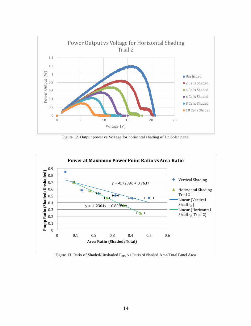
Figure 12. Output power vs Voltage for horizontal shading of UniSolar panel

Figure 13. Ratio of Shaded/Unshaded Pmpp vs Ratio of Shaded Area/Total Panel Area

0

0.2

0.4

0.6

0.8

1

1.2

1.4

0 5 10 15 20 25

Po

wer

Ou

tpu

t (W

)

Voltage (V)

Power Output vs Voltage for Horizontal ShadingTrial 2

Unshaded

2 Cells Shaded

4 Cells Shaded

6 Cells Shaded

8 Cells Shaded

10 Cells Shaded

y = -0.7239x + 0.7637

y = -1.2304x + 0.8039

0

0.1

0.2

0.3

0.4

0.5

0.6

0.7

0.8

0.9

0 0.1 0.2 0.3 0.4 0.5 0.6

Pm

pp

Ra

tio

(S

ha

de

d/

Un

sha

de

d)

Area Ratio (Shaded/Total)

Power at Maximum Power Point Ratio vs Area Ratio

Vertical Shading

Horizontal ShadingTrial 2

Linear (VerticalShading)

Linear (HorizontalShading Trial 2)

15

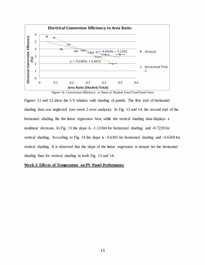
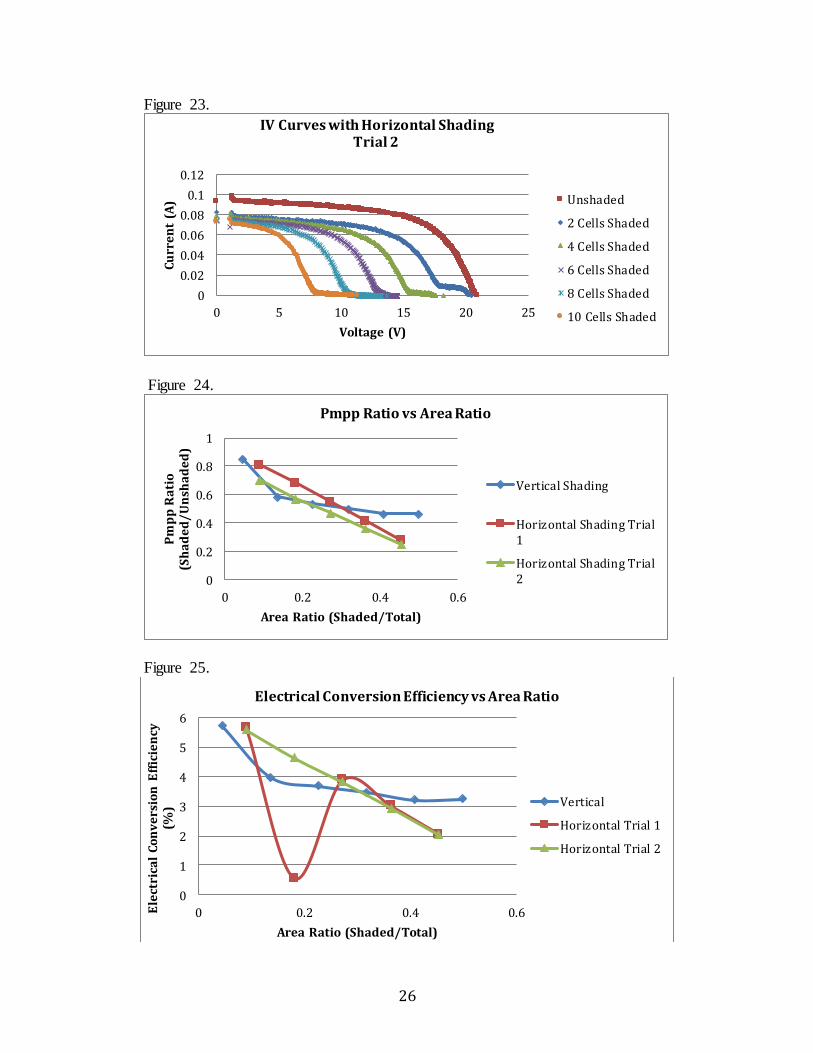
Figure 14. Conversion Efficiency vs Ratio of Shaded Area/Total Panel Area

Figures 11 and 12 show the I-V relation with shading of panels. The first trial of horizontal

shading data was neglected (see week 2 error analysis). In Fig. 13 and 14, the second trial of the

horizontal shading fits the linear regression best, while the vertical shading data displays a

nonlinear decrease. In Fig. 13 the slope is -1.12304 for horizontal shading, and -0.7239 for

vertical shading. According to Fig. 14 the slope is -9.6305 for horizontal shading and -4.6569 for

vertical shading. It is observed that the slope of the linear regression is steeper for the horizontal

shading than for vertical shading in both Fig. 13 and 14.

Week 3: Effects of Temperature on PV Panel Performance

y = -4.6569x + 5.1342

y = -9.6305x + 6.4015

0

1

2

3

4

5

6

0 0.1 0.2 0.3 0.4 0.5 0.6Ele

ctri

cal

Co

nv

ers

ion

Eff

icie

ncy

(%

)

Area Ratio (Shaded/Total)

Electrical Conversion Efficiency vs Area Ratio

Vertical

Horizontal Trial2

16

Figure 15. Pmpp vs Panel Temperature

Figure 16. Electrical Conversion Efficiency vs Panel temperature

y = 0.1401x - 0.103

0

1

2

3

4

5

6

7

8

9

0 5 10 15 20 25

Po

wer

Ou

tpu

t (W

)

Temperature (°C)

Power at Max Power Point vs Panel Temperature

96.32 113.46

98.82 102.72

118.75 131.3

146.91 183.15

214.24 673.52

645.92 262.74

145.8 130.88

123.36 110.53

124.61 127.96

141.75 152.48

141.89 129.49

131.02 133.67

139.8 147.05

159.32 168.1

149.42 164.34

Global Irradiance (W/m2)

y = 0.0089x + 6.7596

0

1

2

3

4

5

6

7

8

9

0 5 10 15 20 25

Ele

ctri

cal C

on

ve

rsio

n E

ffic

ien

cy (

%)

Panel Temperature (°C)

Electrical Conversion Efficiency vs Panel Temperature

96.32 113.46

98.82 102.73

118.75 131.3

146.91 183.15

214.24 645.92

262.74 673.52

145.8 130.88

123.36 110.53

124.61 127.96

141.75 152.48

141.89 129.49

131.02 133.67

139.8 147.05

159.32 168.1

149.42 164.34

Global Irradiance (W/m2)

17

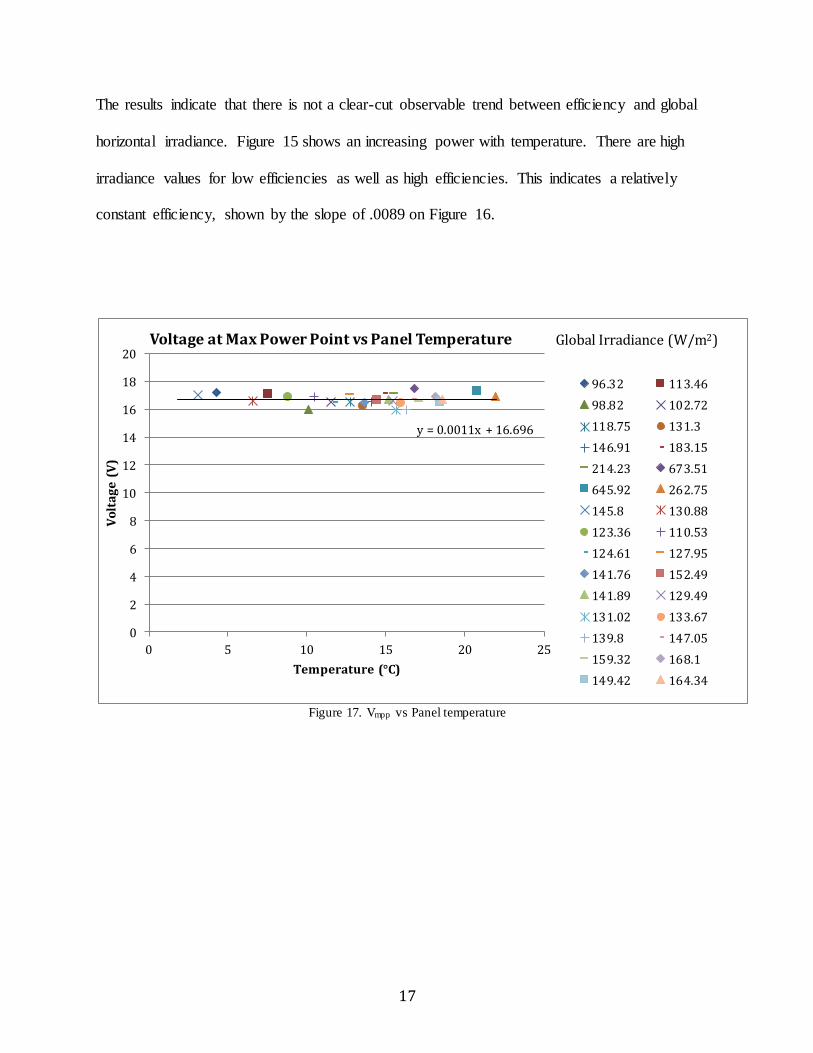
The results indicate that there is not a clear-cut observable trend between efficiency and global

horizontal irradiance. Figure 15 shows an increasing power with temperature. There are high

irradiance values for low efficiencies as well as high efficiencies. This indicates a relatively

constant efficiency, shown by the slope of .0089 on Figure 16.

Figure 17. Vmpp vs Panel temperature

y = 0.0011x + 16.696

0

2

4

6

8

10

12

14

16

18

20

0 5 10 15 20 25

Vo

lta

ge

(V

)

Temperature (°C)

Voltage at Max Power Point vs Panel Temperature

96.32 113.46

98.82 102.72

118.75 131.3

146.91 183.15

214.23 673.51

645.92 262.75

145.8 130.88

123.36 110.53

124.61 127.95

141.76 152.49

141.89 129.49

131.02 133.67

139.8 147.05

159.32 168.1

149.42 164.34

Global Irradiance (W/m2)

18

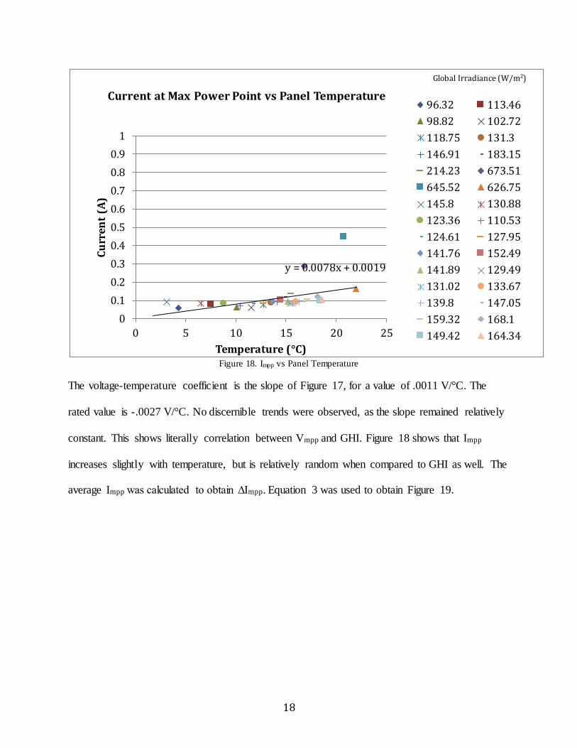
Figure 18. Impp vs Panel Temperature

The voltage-temperature coefficient is the slope of Figure 17, for a value of .0011 V/°C. The

rated value is -.0027 V/°C. No discernible trends were observed, as the slope remained relatively

constant. This shows literally correlation between Vmpp and GHI. Figure 18 shows that Impp

increases slightly with temperature, but is relatively random when compared to GHI as well. The

average Impp was calculated to obtain ∆Impp. Equation 3 was used to obtain Figure 19.

y = 0.0078x + 0.0019

0

0.1

0.2

0.3

0.4

0.5

0.6

0.7

0.8

0.9

1

0 5 10 15 20 25

Cu

rre

nt

(A)

Temperature (°C)

Current at Max Power Point vs Panel Temperature96.32 113.46

98.82 102.72

118.75 131.3

146.91 183.15

214.23 673.51

645.52 626.75

145.8 130.88

123.36 110.53

124.61 127.95

141.76 152.49

141.89 129.49

131.02 133.67

139.8 147.05

159.32 168.1

149.42 164.34

Global Irradiance (W/m2)

19

Figure 19. Corrected Impp vs Panel Temperature

The slope of Figure 19 is the current-temperature coefficient of 0.002 A/°C, as compared to a

rated value of 0.0001 A/°C. Equation 5 was used to calculated corrected power at max power

point. Using equation 2 and corrected power, Figure 20, the graph of corrected efficiency vs

temperature, was obtained.

Figure 20. Corrected Electrical Conversion Efficiency vs Panel Temperature

The corrected conversion efficiency has a more negative slope than the conversion efficiency.

y = 0.0021x + 0.0795

0

0.05

0.1

0.15

0.2

0.25

0 5 10 15 20 25

Co

rrec

ted

Im

pp

(A

)

Temperature (°C)

Corrected Impp versus Temperature

y = -0.0027x + 0.1171

0

0.02

0.04

0.06

0.08

0.1

0.12

0 5 10 15 20 25

Co

rrec

ted

Eff

icie

ncy

Temperature (°C)

Corrected Electrical Conversion Efficiency vs Panel Temperature

20

Discussion with Error Analysis

All measurements obtained by the EKO MP-170 PV Module & Array Tester are accurate

to the order of 10-6. Because these errors are so small compared to the measurements, they can be

neglected. Error propagation for Pmpp Ratio, Power (Figures [12, 13]) yield similar results, and

can be neglected as well.

Week 1:

The figures and the recorded data show that both types of solar panel slightly vary from

the rated (stc) specifications. The rated values were slightly higher than the measured values at

every angle. This could be due to the location where the data was recorded and it could be

caused by the effect of shading on the solar panels. Further, the rated values represent extremely

high efficiency, whereas the measured values do not necessarily represent the maximally

optimizing all factors (such as temperature and irradiance). Voltage should theoretically increase

with solar irradiance because more voltage would be generated when there is more irradiance.

However, Fig. 10 shows a negative relation between voltage and solar irradiance. This could be

explained by other factors affecting the actual voltage that was generated. The voltage decreases

at in extremely slight negative fashion, indicating that a small factor, such as a slight temperature

shift, could have switched the voltage from barely positive to barely negative.

According to the Power at maximum power point vs. Irradiance curves, the maximum

panel power output occurs at an angle of 60 degrees, where irradiance is at the greatest. This

potentially can be attributed to the time of day the data was collected. Because it was late

afternoon, the sun had shifted from the highest point and came in at a lower angle, thus changing

the angle at which the highest irradiance would be observed. The maximum power point occurs

21

on the I-V curve where the curves transitions to a decreasing slope due to power being related to

voltage and current by P = IV.

While taking measurements at different angles, we needed to manually measure the angle

as well as hold the PV panel at the desired angle by hand. Due to these imprecise experimental

techniques the errors associated with PV panel angle are large, +/- 3 degrees. Another type of

error was having negative slope for Vmpp vs. Irradiance is due to application-related errors where

we might have accidentally changed the orientation of the sensors or not accounted for other

factors in the environment. The built in intrinsic errors within the M-170 sensor unit in the

measurement of voltage, current, power, and irradiance are negligible.

Week 2:

The results imply that PV systems are designed so as to maximize the power output even

when shaded. The more rapid decrease in both power at maximum power point and electrical

conversion efficiency for horizontal shading compared to vertical shading (Figures [13, 14]) can

possibly be attributed to the way the individual cells of the PV panel are connected. While

vertically shading, only one cell in each horizontal module (group of two horizontal PV cells)

falls was shaded. That cell falls to a power output of zero, but the power output of the entire

module does not fall to zero. However, while horizontally shading, the entire module is covered,

and thus the entire power output of the full module falls to zero.4 In order to accommodate for

potential power losses due to shading, the PV system would have to be designed to minimize

coverage of full horizontal modules. To accomplish this, the rows of the PV panel could be wired

in series, while the columns could be wired in parallel. According to Ohm’s Law, the connection

in series would maximize output voltage, but would create power-draining loads when individual

22

cells are shaded. Thus, the parallel connection serves to create an equal distribution of voltage to

minimize the power loss due to shading.

The shading was produced by hand with a piece of cardboard. This imperfect technique

could have led to some imperfect shading. To account for this potential error, we assumed a 5%

error. This application related error was due to user interaction with the equipment. Further,

inconsistent irradiance from changing cloud cover affected the data significantly.

Week 3:

The experiment the relative trends between irradiance, temperature, and efficiency on a

PV panel. Theoretically, increased temperatures should lead to decreased efficiency in a PV

panel. However, other factors do play a significant role in affecting the efficiency. There is no

observable trend because of the different changing factors involved in the temperature-based

experiment. The data indicates a slight positive increase in electrical conversion efficiency and

voltage as temperature increases. However, the irradiance was extremely scattered throughout

the dataset, and therefore negates observable correlation between global irradiance and

efficiency. Shifting levels of irradiance due to cloud cover changed ambient air temperatures,

and thus disturbed the data sets. One possible reason for a positive increase in efficiency with

increased temperature is increasing irradiance at a higher rate than temperature. The corrected

electrical conversion efficiency indicates the true correlation between efficiency and

temperature, with a clear decrease in efficiency as temperature increases. Further complications

include water spillage on the solar panel. This not only increases the specific heat capacity, but it

cools down the panel, thus changing the correlative data. The trends for Impp vs Panel

Temperature and Corrected Impp vs Panel Temperature both have a similar positive behavior.

23

Conclusion

This experiment has concentrated on the analysis of the relationship between solar panel

tilt angle, the effect of shading on solar panel performance, and the effect of temperature on PV

performance. The maximum power output for Kyocera solar panel was found to be 9.96W at the

tilt angle of 60º, where the solar irradiance has a positive correlation with power output. The

experiment had shown that horizontal shading had a more significant impact on power output

than vertical shading. The experiment also shows that temperature has a negative correlation

with electrical conversion efficiency. Changes in any factors affecting power output can

significantly change the result. Therefore, PV systems must be designed to accommodate a

balance between the least amount of horizontal shading, the most irradiance, and the least

possible panel temperature.

24

References

1. "Solar Angles and Tracking Systems." Solar Angles and Tracking Systems - Lesson -

Www.TeachEngineering.org. N.p., 05 Feb. 2014. Web. 02 Feb. 2014.

2. "Part II – Photovoltaic Cell I-V Characterization Theory and LabVIEW Analysis Code." -

National Instruments. N.p., 10 May 2012. Web. 02 Feb. 2014.

3. Kleissl, Jan, and R. A. De Callafon. "Laboratory Course Website, Dept. of Mechanical and

Aerospace Engineering at UCSD." Laboratory Course Website, Dept. of Mechanical and

Aerospace Engineering at UCSD. N.p., 18 Feb. 2013. Web. 02 Feb. 2014.

4. “Solar Electronics, Panel Integration and Bankability Challenge.” GreenTechMedia.

http://www.greentechmedia.com/articles/read/solar-electronics-panel-integration-and-the-

bankability-challenge. 06 Feb. 2014.

25

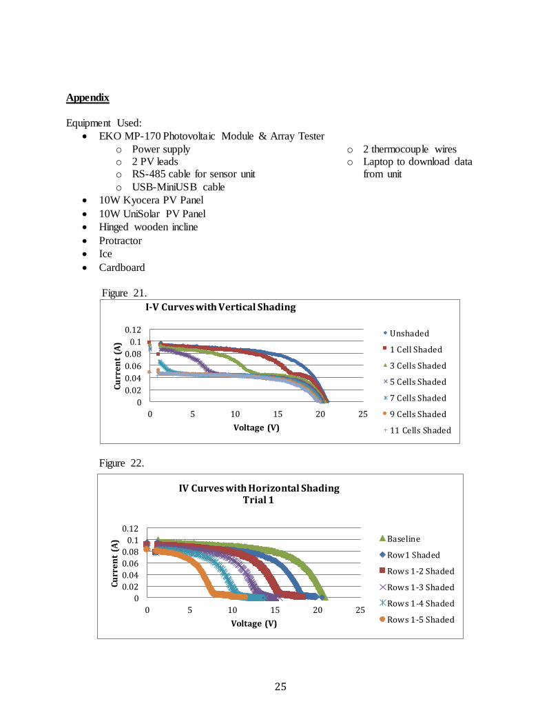
Appendix

Equipment Used:

EKO MP-170 Photovoltaic Module & Array Tester

o Power supply o 2 PV leads o RS-485 cable for sensor unit

o USB-MiniUSB cable

o 2 thermocouple wires o Laptop to download data

from unit

10W Kyocera PV Panel

10W UniSolar PV Panel

Hinged wooden incline

Protractor

Ice

Cardboard

Figure 21.

Figure 22.

0

0.02

0.04

0.06

0.08

0.1

0.12

0 5 10 15 20 25

Cu

rre

nt

(A)

Voltage (V)

I-V Curves with Vertical Shading

Unshaded

1 Cell Shaded

3 Cells Shaded

5 Cells Shaded

7 Cells Shaded

9 Cells Shaded

11 Cells Shaded

0

0.02

0.04

0.06

0.08

0.1

0.12

0 5 10 15 20 25

Cu

rre

nt

(A)

Voltage (V)

IV Curves with Horizontal ShadingTrial 1

Baseline

Row1 Shaded

Rows 1-2 Shaded

Rows 1-3 Shaded

Rows 1-4 Shaded

Rows 1-5 Shaded

26

Figure 23.

Figure 24.

Figure 25.

0

0.02

0.04

0.06

0.08

0.1

0.12

0 5 10 15 20 25

Cu

rre

nt

(A)

Voltage (V)

IV Curves with Horizontal ShadingTrial 2

Unshaded

2 Cells Shaded

4 Cells Shaded

6 Cells Shaded

8 Cells Shaded

10 Cells Shaded

0

0.2

0.4

0.6

0.8

1

0 0.2 0.4 0.6

Pm

pp

Ra

tio

(S

ha

de

d/

Un

sha

de

d)

Area Ratio (Shaded/Total)

Pmpp Ratio vs Area Ratio

Vertical Shading

Horizontal Shading Trial1

Horizontal Shading Trial2

0

1

2

3

4

5

6

0 0.2 0.4 0.6Ele

ctri

cal

Co

nv

ers

ion

Eff

icie

ncy

(%

)

Area Ratio (Shaded/Total)

Electrical Conversion Efficiency vs Area Ratio

Vertical

Horizontal Trial 1

Horizontal Trial 2

27

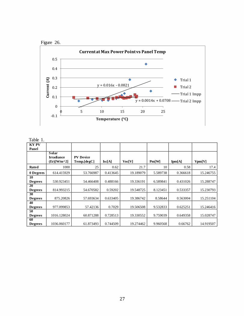
Figure 26.

Table 1. KY PV

Panel

Solar

Irradiance

(Er)[W/m^2]

PV Device

Temp.[degC] Isc[A] Voc[V] Pm[W] Ipm[A] Vpm[V]

Rated 1000 25 0.62 21.7 10 0.58 17.4

0 Degrees 614.415929 53.766987 0.413645 19.189079 5.589738 0.366618 15.246755

10

Degrees 530.923451 54.466408 0.488166 19.336191 6.589841 0.431026 15.288747

20

Degrees 814.993215 54.670582 0.59202 19.548725 8.123451 0.533357 15.230793

30

Degrees 875.20826 57.693634 0.633405 19.386742 8.58644 0.563004 15.251104

40

Degrees 977.099853 57.42136 0.7029 19.506508 9.532833 0.625251 15.246416

50

Degrees 1016.128024 60.871288 0.728513 19.330552 9.759039 0.649358 15.028747

60

Degrees 1036.060177 61.873493 0.744509 19.274462 9.960568 0.66762 14.919507

y = 0.016x - 0.0821

y = 0.0014x + 0.0708

-0.1

0

0.1

0.2

0.3

0.4

0.5

0 5 10 15 20 25

Cu

rre

nt

(A)

Temperature (°C)

Current at Max Power Point vs Panel Temp

Trial 1

Trial 2

Trial 1 Impp

Trial 2 Impp