National Conference with International Participation

ENGINEERING MECHANICS 2008

Svratka, Czech Republic, May 12 – 15, 2008

EXPERIMENTAL STUDY OF WIND LOAD ON RAILWAY-STATION

OBEJCTS

D. Zachoval* , M. Jirsák

**

Summary: The case-study of wind load on innovation railway-station objects was

performed using VZLÚ boundary layer wind tunnel. The results of this experiment

were processed to mean values, its standard deviations and to the gust peak

factors. Spectral analysis of this signal was made for each tap with extreme value

of the gust peak factor. Dimensionless values of the pressure coefficient were

related to reference dynamic pressure conformable with Eurocode 1.

1. Introduction

The paper outlines case-study of wind load acting on low-rise railway-station roofs. The

innovation is concerned of new roof structure over the railway-station platforms. Structural

analysis of the railway-station roofs uses a code for the wind load assessment. The code

includes parameters of wind flow above the flat uniformly rough terrain (FUR) without

specific buildings. As the railway station finds in city center of Salzburg (with substantially

higher buildings in near vicinity), oncoming flow structure differs significantly with wind

direction.

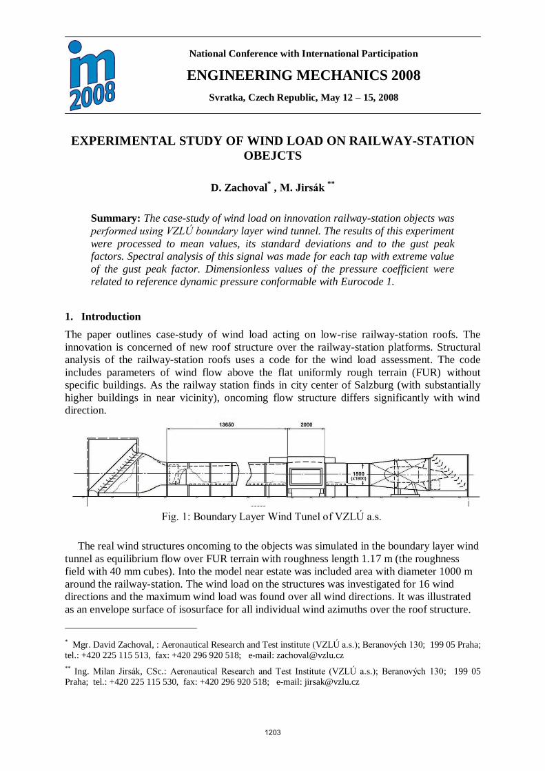
The real wind structures oncoming to the objects was simulated in the boundary layer wind

tunnel as equilibrium flow over FUR terrain with roughness length 1.17 m (the roughness

field with 40 mm cubes). Into the model near estate was included area with diameter 1000 m

around the railway-station. The wind load on the structures was investigated for 16 wind

directions and the maximum wind load was found over all wind directions. It was illustrated

as an envelope surface of isosurface for all individual wind azimuths over the roof structure.

* Mgr. David Zachoval, : Aeronautical Research and Test institute (VZLÚ a.s.); Beranových 130; 199 05 Praha;

tel.: +420 225 115 513, fax: +420 296 920 518; e-mail: zachoval@vzlu.cz

** Ing. Milan Jirsák, CSc.: Aeronautical Research and Test Institute (VZLÚ a.s.); Beranových 130; 199 05

Praha; tel.: +420 225 115 530, fax: +420 296 920 518; e-mail: jirsak@vzlu.cz

Fig. 1: Boundary Layer Wind Tunel of VZLÚ a.s.

1203

2. The Atmospheric Boundary Layer (ABL) simulation

The simulation of ABL in the wind tunnel (see Fig. 1) above the terrain with urban roughness

for this experiment uses the roughness field in net fetch of 11.4 m. The Counihan vortex

generator is situated in front of the roughness field composed from battery of elliptic knives in

combination with castellated wall.

Boundary layer properties were tested over the section of 700 mm upwind the end of cube

fetch. The vertical distribution of mean velocity and turbulence intensity were checked above

centre of turntable and in lateral distance ±600 mm from it. The Fig. 2 introduces these mean

velocity and the standard deviation profiles normalized by friction velocity (U/u* and u/u*).

Span average value of model roughness length z0,m = 4.7 mm derived from the three vertical

velocity profiles is appropriate to roughness length z0 = 1.17 m in full scale.

Power spectrum in Fig. 3 monitors the distribution of turbulent energy (that of longitudinal

component) in dependence on the dimensionless frequency as result of the FFT processing.

The region of power dependence on frequency is exhibited, proper to inertial sub-range,

0

2

4

6

8

10

12

14

10 100 1000

U/u*

uvar/u*

z .d

Velocity profiles

normalized by local u* value

(U/u*)-600 (U/u*)y=0 (U/u*)600

4 ul/u* 4 uc/u* 4 ur/u*

2,5 ln(z/5) 2,5 ln(z/3,5) 2,5 ln(z/5,3)

Fig. 2: Incident flow

1204

showing energy equilibrium state of the boundary layer.

3. Model of the railway-station

The model (VZLÚ production) was designed according the customer data (transferred to

convenient software), complied with available satellite pictures. The passive estate members

were machined from synthetic wood while R.S. roofs were manufactured as carbon fibre

composite.

The pressure taps (218 pieces) were disposed over the upper and lower roof surfaces and

connected with pressure scanner Easterline (model 16TC, range ±10”WC) by polyethylene

tubing within inner diameter of 1 mm and 800 mm length. The frequency response of the

measuring line (see Fig. 8) was measure, which was used later for signal coerrection at its

processing. It was measured as the response of the line to the pressure pulse with very short

duration (approximately 2 ms).

0.0001

0.001

0.01

0.1

1

0.01 0.1 1 10

f.Su(f)/u2

f Lu,x/U(z)

Power spectral density (the urban simulation)

z=75

z=150

z=300

z=450

Kolmogoroff

law

Fig. 3: Power spectral density, Lu,x is integral length scale of turbulence

Fig. 4: Model of the Salzburg railway-station with surrounding estate

1205

4. Set of the equipment

The signals were sampled with frequency 3kHz during time period 30 s each pressure tap and

it were filtered by low-pass analogue filter with limit frequency approximately 290 Hz.

5. The similarity criteria

The modeled case is clearly confined to the atmospheric surface layer range whose structure

the wind tunnel is able to product quite consistently. Thickness of the ASL (roughly 15% of

ABL) represents lower 70÷100 m layer where shear stress distribution is nearly constant as

follows from the ASL definition. All the well-known characteristics of ASL over flat

uniformly rough terrain are valid only on heights overcoming tops of roughness elements,

forming its statistical planar homogeneity.

Existence of the “fully rough turbulent flow” (it is always present in the atmosphere) is

conditioned in BL wind tunnel by sufficient velocity with respect to magnitude of roughness

elements. The similarity is attained at sufficient value of “roughness Reynolds number” Re*

𝑅𝑒∗ = 𝑢∗𝑧0

𝜈> 𝑅𝑒𝑘

∗, where

u* .. is friction velocity, z0 .. roughness length and ν .. is kinematic viscosity. Taking critical

value of 𝑅𝑒𝑘∗ ≈ 2,5 (ASCE man. 1969) and our mean z0 = 4.7 mm and u*/UG ≈ 0,0674 we get

𝑢∗ > 2.515

4.7𝐸−3= 0.00798𝑚 𝑠 whence 𝑈𝐺 > 0,184 𝑚 𝑠 .

The requirement is ample satisfied with actual experimental value of the gradient velocity

UG≈ 15 m/s.

Fig. 5: Numbering of the pressure taps on bottom and top site of the roof structure

(1)

1206

6. Results

The pressure values on both sides of the roof structure were measured as different pressure

Δpi between the wind pressure at the i-tap on the roof structure pw,i and the static pressure in

the wind tunnel pstat.

∆𝑝𝑖 = 𝑝𝑤 ,𝑖 − 𝑝𝑠𝑡𝑎𝑡

The static pressure was taken from the Prandtl probe static orifice, situated above the

boundary layer upwind the model section of the wind tunnel.

There were several problems. At first, reference static pressure in relatively smooth flow

above the boundary layer is different from that in very disturbed flow in the boundary layer

bottom. In the consequence, the sign of resulting pressure coefficients was mostly negative.

This dificult was removed expressing the differences between upper and lower roof surface.

𝑝𝑖 = ∆𝑝𝑖 ,𝑙𝑜𝑤𝑒𝑟 − ∆𝑝𝑖 ,𝑢𝑝𝑝𝑒𝑟 ,

where pi represents force at the i upper pressure taps. The forces ensuing from positive value

of pi pulls the roof structure up and force ensuing from negative value of pi pushes the roof

down.

The results of the wind load measurement were mean pressure coefficients 𝑐 𝑝 ,𝑖 . It is

defined as ratio

𝑐 𝑝 ,𝑖 = 𝑝 𝑖

𝑞𝑟𝑒𝑓

where qref is reference dynamic pressure. It was request to of compare the experimental

dimensionless results with the values developed from codes related to wind at the height of 10

m above earth. Therefore the value of dynamic head on height of z = 40 mm developed from

the scaled profile of mean velocity of incident flow. Uref = 6.09 m/s i.e. qref ≈ 21.45 Pa was

used for the pressure coefficient cp,i final evaluation.

The statistical processing of the pressure signal gave to following values of the pressure.

Mean pressure 𝑝 i, its standard deviation pi,SD, maximum 𝑝𝑖 and minimum peak 𝑝𝑖 of the

pressure signal.

Spectral analysis of the pressure signal was done in the case when the its negative peak

was at least four times higher than its standard deviation.

It is ensuing from equation

𝑝 𝑖 = 𝑝𝑖 + 𝑔𝑝𝑖,𝑆𝐷 𝑔 = 𝑝 𝑖− 𝑝 𝑖

𝑝𝑖 ,𝑆𝐷

where g is gust peak factor.

The maximum wind load on roof structure is depicted in Fig. 6 as an envelope of the wind

loads proper to all measured wind directions.

(2)

(4)

(3)

(5)

1207

Examples of pressure spectra are in Fig. (9 –

12). The examples were chosen for the peak

factors proper to the maximal wind acting on the

structure. The pressure spectra were prepared for

the all records where |g| ≥4. Spectra of the

particular cases are labelled by proper angle/tap

combination. Here it should mention occurrence of

the disturbing peaks caused either by standing

acoustic waves in the wind channel, or to the

frequencies induced by four fan blades.

Fig. 6: maximum wind load on roof structure, the positive value of the cp represents the

suction

Fig. 7: Gust peak factor, for maximum wind loading pressure coeficinets

Fig. 8: Response of the measuring

line

1208

It is visible that with respect of possible elimination of the disturbing peaks one could

accept the spectra to be valid in frequencies approximately from 0.3 Hz up to roughly 100 Hz.

This limit of the modeled frequency answers to lower frequency limit in the case of full scale.

This follows from Strouhal number similarity:

𝑆𝑕 = 𝑓𝑚 𝐿𝑚

𝑈𝐺 𝑚=

𝑓𝐹𝑆 𝐿𝐹𝑆

𝑈𝐺 𝐹𝑆.

At the actual length scale Lm/LFS = 1/205 and supposed (UG)m/(UG)FS = 1/5 for strong wind,

we get

𝑓𝐹𝑆 𝑚𝑎𝑥 = 𝑓𝑚 𝑚𝑎𝑥

𝐿𝑚

𝐿𝐹𝑆

𝑈𝐺 𝐹𝑆 𝑈𝐺 𝑚

= 1001

2505 = 2𝐻𝑧.

Variability of the spectral distribution of fluctuating energy for the individual taps of this

spectra measurement is evident.

Fig. 9: Spectrum of pressure record on the

point 4 (0° wind angle) Fig. 10: Spectrum of pressure record on the

135 (225° wind angle)

Fig. 11: Spectrum of pressure record on the

point 116 (67.5° wind angle)

Fig. 12: Spectrum of pressure record on the

point 117 (67.5° wind angle)

(6)

(7)

1209

7. Pressure results and their discussion

Resulting pressure coefficients cp,i as they were measured on the taps are found within range

form -0,62 to 1.76. Their values are importantly influenced by estate environs, depending on

wind angle as it is documented by following:

Surveying Fig. 6 we can see that the maximal positive pressure differences (acting upwards)

appear on northern ends of platform roofs at angles of about 247.5°, where wind comes from

free space above rails (NE wind) and turns up on the roof tips with cp,i approaching the

absolute maximum with values of about 1.8 (taps No.39 and 114 found close the cutouts of

northern roof tips). The next area of increased positive pressure (lower, about cp≈1.2) is found

near the front part of the hall ridge appearing at wind angles of 202.5°.

The points with high gust peak factor are just at the ends of the roof structure. The wind

can flutter with the roof structure. Critical dynamic load will occur when frequency of the

flutter approaches the natural frequency of the roof structure.

8. Conclusions

Experiments focused on wind load acting on the low railway-station objects which are

submerged in the higher surrounding buildings represent very demanding task with respect of

quite different oncoming wind structure coming from different wind angles, mostly

containing wakes of near buildings which changes mean static pressure on the site. Another

complication following Salzburg railway-station modelling arises in the consequence of

surrounding orography, causing difficulties in connecting of wind tunnel results with

meteorological statistics measured on site of Salzburg airport much less affected by orography

effects. Simulated wind approached the complete model from flat uniformly rough terrain (its

structure) was modified only by passive building environs. In the sense, assessment of actual

wind loading on the parts of railway-station structure, as well as the approach of pedestrian

wind conditions are valid, of course, without directional changes of the gradient velocity

caused by the orography.

The experimental assessment of the wind loading on complex roof structure is important

because the code includes just basic shape of the roofs and just two basic wind directions. The

code calculated with wind coming from flat uniformly rough terrain and it doesn’t include

specific estate at vicinity of the measured object.

The complete wind tunnel model with the modelled neighbouring estate (from aside the

FUR simulation) solves the tasks of dynamic wind acting on railway-station objects with

much higher accuracy and fine details than it would do the wind codes, so as then any CFD

model.

References

ASCE Manuals & Reports on Eng. Practice, No.67 (1999) Wind Tunnel Studies of Buildings,

American Society of Civil Engineers, Reston, Virginia.

Claës Dyrbye, Svend O. Hansen (1996), Wind Load on Structures, Original published in

Danish.

1210

ČSN EN 1991-1-4 Zásady navrhování a zatížení konstrukcí – Část 2-4 Zatížení konstrukcí –

Zatížení větrem

Jirsák M., Zachoval D.: Experimental study on innovation project of Salzburg railway

station, VZLÚ, R 4152/07

Rep. VZLÚ V-1708/2000 Jirsak M. et al.: The completing of the simulation development

(Project MPO FB-C/85/99 RC1.6, in Czech)

1211