experiments on free-surface turbulence · experiments on free-surface turbulence / by ralph...
TRANSCRIPT

Experiments on free-surface turbulence
Savelsberg, R.
DOI:10.6100/IR609526
Published: 01/01/2006
Document VersionPublisher’s PDF, also known as Version of Record (includes final page, issue and volume numbers)
Please check the document version of this publication:
• A submitted manuscript is the author's version of the article upon submission and before peer-review. There can be important differencesbetween the submitted version and the official published version of record. People interested in the research are advised to contact theauthor for the final version of the publication, or visit the DOI to the publisher's website.• The final author version and the galley proof are versions of the publication after peer review.• The final published version features the final layout of the paper including the volume, issue and page numbers.
Link to publication
General rightsCopyright and moral rights for the publications made accessible in the public portal are retained by the authors and/or other copyright ownersand it is a condition of accessing publications that users recognise and abide by the legal requirements associated with these rights.
• Users may download and print one copy of any publication from the public portal for the purpose of private study or research. • You may not further distribute the material or use it for any profit-making activity or commercial gain • You may freely distribute the URL identifying the publication in the public portal ?
Take down policyIf you believe that this document breaches copyright please contact us providing details, and we will remove access to the work immediatelyand investigate your claim.
Download date: 13. Jul. 2018

Experiments on Free-Surface
Turbulence
PROEFSCHRIFT
ter verkrijging van de graad van doctor aan deTechnische Universiteit Eindhoven, op gezag vande Rector Magnificus, prof.dr.ir C.J. van Duijn,voor een commissie aangewezen door het Collegevoor Promoties in het openbaar te verdedigen op
donderdag 8 juni 2006 om 16.00 uur
door
Ralph Savelsberg
geboren te Kerkrade

Dit proefschrift is goedgekeurd door de promotoren :
prof.dr.ir. W. van de Waterenprof.dr.ir. G.J.F. van Heijst
Dit werk maakt deel uit van het onderzoeksprogramma van de Stichting voorFundamenteel Onderzoek der Materie (FOM), die financieel wordt gesteunddoor de Nederlandse Organisatie voor Wetenschappelijk Onderzoek (NWO).
Omslag / Cover: Yellowstone Lake, Yellowstone National Park, Wyoming,USA. Foto met dank aan / Photograph courtesy of Maikel van Hest.Omslag ontwerp / Cover design : Paul Verspaget & Carin Bruinink Grafischevormgeving.Druk / Printed by : Universiteitsdrukkerij Technische Universiteit Eindhoven.
CIP-DATA LIBRARY TECHNISCHE UNIVERSITEIT EINDHOVEN
Savelsberg, Ralph
Experiments on Free-Surface Turbulence / by Ralph Savelsberg. –Eindhoven : Technische Universiteit Eindhoven, 2006. –Proefschrift.ISBN-10: 90-386-2501-4ISBN-13: 978-90-386-2501-0NUR 926Trefwoorden : turbulentie / turbulente stroming / lasersnelheidsmetingen /optische meetmethoden /hydrodynamische golvenSubject headings : turbulence / turbulent flow / water waves / laservelocimetry / shape measurement

Contents
1 Introduction 11.1 Turbulence . . . . . . . . . . . . . . . . . . . . . . . . . . . . . . 11.2 Free-surface deformations . . . . . . . . . . . . . . . . . . . . . . 31.3 Experiments . . . . . . . . . . . . . . . . . . . . . . . . . . . . . . 41.4 Overview of this thesis . . . . . . . . . . . . . . . . . . . . . . . . 7
2 Free-surface turbulence 92.1 Boundary conditions at a free surface . . . . . . . . . . . . . . . 9
2.1.1 Linear gravity-capillary waves . . . . . . . . . . . . . . . . 122.1.2 Sub-surface structures . . . . . . . . . . . . . . . . . . . . 15
2.2 Phenomenology of free-surface turbulence . . . . . . . . . . . . . 192.2.1 Turbulence statistics under a free surface. . . . . . . . . . 192.2.2 Free-surface deformations . . . . . . . . . . . . . . . . . . 222.2.3 The generation of waves by turbulence . . . . . . . . . . . 25
3 Basic properties of the turbulence 273.1 Active-grid-generated turbulence . . . . . . . . . . . . . . . . . . 27
3.1.1 Grid geometry . . . . . . . . . . . . . . . . . . . . . . . . 293.1.2 Forcing protocols . . . . . . . . . . . . . . . . . . . . . . . 31
3.2 Laser Doppler Velocimetry . . . . . . . . . . . . . . . . . . . . . . 333.2.1 Principle of LDV . . . . . . . . . . . . . . . . . . . . . . . 333.2.2 The set-up for Laser-Doppler measurements . . . . . . . . 36
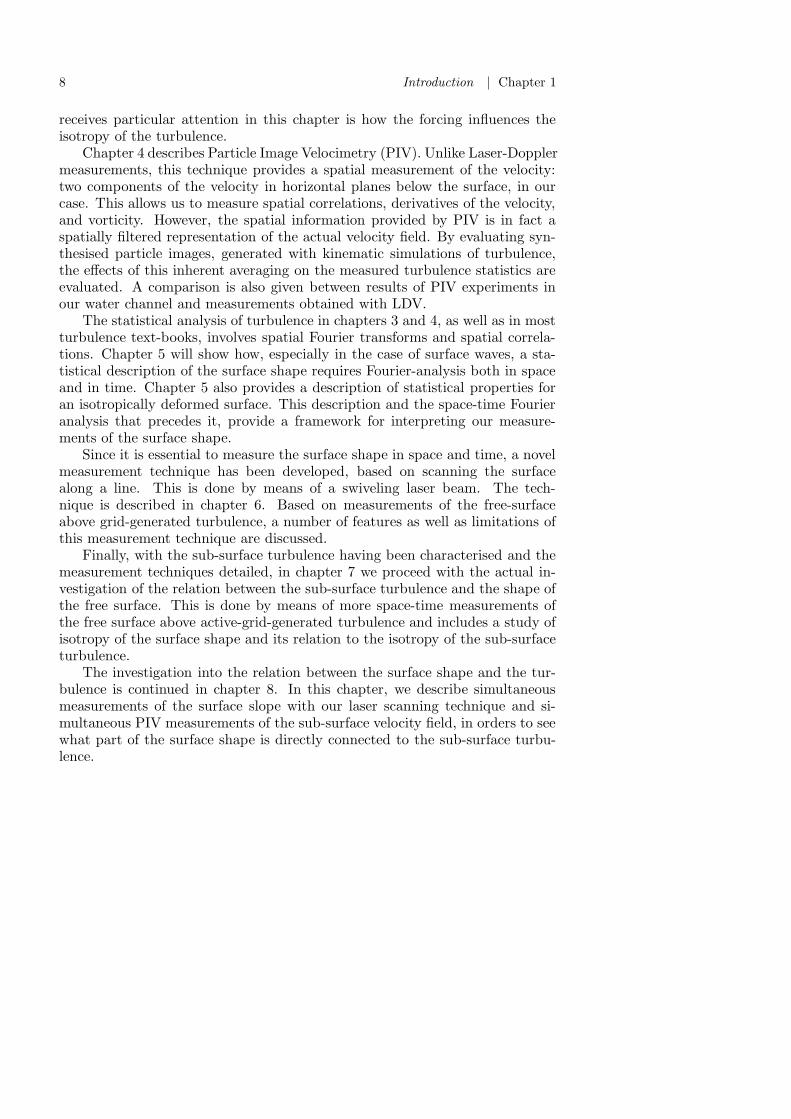
3.3 Properties of the turbulence . . . . . . . . . . . . . . . . . . . . . 393.3.1 Homogeneity . . . . . . . . . . . . . . . . . . . . . . . . . 393.3.2 Turbulent scales . . . . . . . . . . . . . . . . . . . . . . . 423.3.3 Isotropy . . . . . . . . . . . . . . . . . . . . . . . . . . . 46
3.4 Conclusions . . . . . . . . . . . . . . . . . . . . . . . . . . . . . . 49
4 Measuring turbulence properties with PIV 514.1 Introduction . . . . . . . . . . . . . . . . . . . . . . . . . . . . . . 514.2 The principle of PIV . . . . . . . . . . . . . . . . . . . . . . . . . 534.3 Inherent filtering by PIV . . . . . . . . . . . . . . . . . . . . . . . 58

ii CONTENTS
4.3.1 A description of the filter . . . . . . . . . . . . . . . . . . 584.3.2 The effect of spatial averaging on turbulence statistics. . . 59
4.4 Applying PIV to simulated velocity fields . . . . . . . . . . . . . 664.4.1 Kinematic simulations . . . . . . . . . . . . . . . . . . . . 664.4.2 Generating realistic particle images . . . . . . . . . . . . . 694.4.3 Comparison of turbulence statistics . . . . . . . . . . . . . 724.4.4 The influence of particle loss . . . . . . . . . . . . . . . . 76
4.5 Experiments . . . . . . . . . . . . . . . . . . . . . . . . . . . . . . 794.5.1 A comparison of PIV and LDV measurements . . . . . . . 804.5.2 Isotropy in horizontal planes . . . . . . . . . . . . . . . . 84
4.6 Conclusions . . . . . . . . . . . . . . . . . . . . . . . . . . . . . . 87
5 A statistical description of the surface shape 895.1 Basic definitions . . . . . . . . . . . . . . . . . . . . . . . . . . . 895.2 Statistics of the slope at a point . . . . . . . . . . . . . . . . . . . 915.3 Slope statistics in time and space . . . . . . . . . . . . . . . . . . 93
5.3.1 Dispersive surface waves . . . . . . . . . . . . . . . . . . . 945.3.2 Spectra in time and space . . . . . . . . . . . . . . . . . . 965.3.3 Isotropy in the surface slopes . . . . . . . . . . . . . . . . 98
6 Measuring the slope of the free surface 1036.1 Introduction . . . . . . . . . . . . . . . . . . . . . . . . . . . . . . 1036.2 Point measurements of the surface slope . . . . . . . . . . . . . . 1056.3 Measuring the slope in space and time . . . . . . . . . . . . . . . 107
6.3.1 Set-up for slope measurements along a line . . . . . . . . 1076.3.2 Synchronisation . . . . . . . . . . . . . . . . . . . . . . . . 1086.3.3 Data processing . . . . . . . . . . . . . . . . . . . . . . . . 112
6.4 Assessment of the surface scanning method . . . . . . . . . . . . 1146.5 Conclusions . . . . . . . . . . . . . . . . . . . . . . . . . . . . . . 119
7 The nature of the surface ripples 1217.1 Spectra and correlations in time and space . . . . . . . . . . . . . 121
7.1.1 Correlation functions . . . . . . . . . . . . . . . . . . . . . 1287.1.2 The surface spectrum . . . . . . . . . . . . . . . . . . . . 129
7.2 Isotropy . . . . . . . . . . . . . . . . . . . . . . . . . . . . . . . . 1307.3 Synthetic surfaces . . . . . . . . . . . . . . . . . . . . . . . . . . 1337.4 Conclusions . . . . . . . . . . . . . . . . . . . . . . . . . . . . . . 135
8 Correlating the sub-surface turbulence and the surface shape 1378.1 Correlation between turbulence and the surface shape . . . . . . 139
8.1.1 Taylor’s hypothesis for free-surface turbulence . . . . . . . 1408.1.2 Calculating the elevation . . . . . . . . . . . . . . . . . . 144
8.2 Combining PIV and surface slope measurements . . . . . . . . . 1468.3 A test case: vortex shedding . . . . . . . . . . . . . . . . . . . . . 149

Contents iii
8.4 Grid-generated turbulence . . . . . . . . . . . . . . . . . . . . . . 1558.5 Conclusions . . . . . . . . . . . . . . . . . . . . . . . . . . . . . . 160
9 General conclusions 163
Summary 173
Samenvatting 175
Dankwoord / Acknowledgements 177
Curriculum Vitae 179


1
Introduction
1.1 Turbulence
In general, the words turbulent and turbulence are used to describe situationsthat are wild, stormy, tumultuous, agitated, and above all unpredictable. To acertain degree, these descriptions are also true for turbulent flows. Most flows,both in nature and in technological applications, are turbulent. Atmosphericflow is turbulent, which is one of the causes of the unpredictable nature ofour weather. Turbulence in the seas and oceans directly impacts our climate,and affects the distribution of, for instance, plankton, but also of algae andpollution. The chaotic motion inherent to turbulence is used for stirring andmixing chemicals in industrial applications, and, on a much smaller scale, indistributing milk and or sugar through a cup of tea. Combustion, for instancein power plants and car engines, is a turbulent process. In order to understandall these processes, and in case of technological applications in order to improvetheir efficiency, understanding turbulence is essential.
The equation of motion for a fluid is the well-known Navier-Stokes equation,which in essence is Newton’s second law of motion applied to a fluid parcel ∗:
Du(x, t)
Dt= −1
ρ∇p(x, t) + g + ν∇2u(x, t). (1.1)
In this equation, u(x, t) is the fluid velocity at a location x and a time t, ρ isthe density of the fluid, p(x, t) is the pressure, g is the gravitational accelera-tion, and ν is the (kinematic) viscosity of the fluid. In principle, this equation,together with the continuity equation: ∇ · u = 0, fully describes the motionof a fluid, including that in turbulent flows. However, even though the basicequations that describe the fluid motion are known and have been known for
∗Already indicating some limitations, this equation as formulated here is only validfor a homogeneous, incompressible, and Newtonian fluid, without background rotation.

2 Introduction | Chapter 1
more than a century, turbulence essentially is an unsolved problem. The equa-tions allow solutions of a bewildering complexity and exact solutions have onlybeen found for rare and decidedly non-turbulent cases.
A feature of turbulent flows is the occurrence of structures, often callededdies, associated with rapidly fluctuating vorticity. The motion in a turbulentflow occurs over a wide range of length- and time scales. By vortex-stretchingand vortex-breakup, two non-linear processes, the energy that is contained inlarge scale eddies is transferred to smaller structures, in what has become knownas the energy cascade. Because of the unpredictable and seemingly random mo-tions in turbulence, almost all descriptions and measurements of turbulence dealwith statistical quantities such as averages, variances, correlation functions, andenergy spectra. A major breakthrough in the development of a statistical de-scription of turbulence was the work by A.N. Kolmogorov. Based on the notionof the energy cascade, he postulated that for strong turbulence the energy thatis transferred from larger to smaller scales is dissipated by viscous effects onlyon the smallest scales in the turbulence. Accordingly, the turbulence statis-tics on the smallest scales depend on both the energy dissipation rate ε andthe viscosity of the fluid. By dimensional arguments Kolmogorov found that,thus, these smallest scales were of a size: η = (ν3/ε)1/4. He also hypothe-sised that, since viscosity does not play a role on larger scales, the statistics forthese larger scales depend only on the energy dissipation rate. From this hederived his now-famous five-third law for the turbulent energy spectrum. Thedefinition of the energy spectrum, which we will call E(k), is based on Fourier-analysis: E(k)dk is the kinetic energy density in the velocity field containedin Fourier-modes with wavenumbers between k and k + dk. By dimensionalanalysis, Kolmogorov concluded that for scales in the flow larger than η (butsmaller than the largest scales) the energy spectrum shows algebraic scalingwith a scaling exponent of −5/3:
E(k) = Cε2
3 k− 5
3 , (1.2)
with a constant C that is most probably universal, but for which no theoryexists, unless the turbulence problem is solved. This scaling behaviour hassince been observed in a wide variety of turbulent flows, including very largescale flows in the atmosphere and smaller scale flows in, for instance, windtunnels. This theory will be the framework for interpreting our turbulencemeasurements. In particular, our question will be how this multitude of scalesin turbulence is reflected in the size of structures that can be found at thefree surface of the flow. A more detailed description of the theory and itsconsequences and limitations can be found in turbulence textbooks, such as thebooks by Frisch (1995) and Pope (2000).

1.2 | Free-surface deformations 3
1.2 Free-surface deformations
Turbulent flows in seas and oceans, as well as flows in rivers and channels, forinstance, are special in the sense that they have a free surface. Turbulence closeto the interface between water and air behaves very differently from turbulencenear fixed walls, such as the walls of a flow channel or the ocean floor. One of themost obvious features of the air-water interface is that it is deformable. Thesmall-scale roughness of the ocean’s surface determines the exchange of heatand mass between the atmosphere and the ocean. These transport processesare crucial for the global distribution of momentum, heat and chemical species.
By far the most common type of surface deformation to occur in nature arewaves, ranging from tiny thermally driven capillary waves, with wavelengthsof a few micrometers and amplitudes of a few nanometers (Aarts et al., 2004),to monstrous waves induced by earth-quakes, that can travel across the entireglobe and that can reach heights of several meters (Titov et al., 2005). Amore common source of waves on the sea or ocean surface is turbulence in thewind above it, and pressure fluctuations and fluctuating shear stresses on thesurface associated with this. The interaction of waves and wind is a complicatedproblem that has been studied for decades (see Phillips, 1957) and is in factstill being investigated.
The shape of the surface is determined by a delicate balance between verticalacceleration and pressure in the flow below the surface on one hand, and gravityand interfacial tension, i.e. stresses associated with surface curvature, on theother hand. Which force dominates this balance depends on the scale of thedeformation. Generally, for large scale surface deformations, gravity balancesvertical accelerations in the fluid, whereas for smaller scales surface tensionplays a more important role. In a recent paper, Brocchini & Peregrine (2001)have classified the different types of structures and the behaviour that can occurat a free surface above turbulent flow, depending on which force dominates.Structures, other than waves, commonly seen on a free surface above turbulenceare scars; sharp lines on the surface, most often associated with up- or down-welling of fluid at the surface. Additionally, low pressure in the core of sub-surface eddies can lead to dimples in the surface. These too are fairly commonstructures, visible in the wake behind bridge pillars in a river, behind oars ona boat, or in a cup of tea that is stirred with a spoon. Brocchini & Peregrine(2001) distinguish four different regimes of free surface distortions as a resultof sub-surface turbulence, depending on a typical length-scale L and typicalvelocity scale U of the turbulence. Based on these scales, they define twodimensionless numbers: the Froude number, which is a measure of the potentialenergy due to gravity relative to the kinetic energy in the flow:
Fr =U√2gL
, (1.3)
where g is the gravitational acceleration, and the Weber number, which gauges

4 Introduction | Chapter 1
the balance between inertial and surface tension forces:
We =U2Lρ
2σ, (1.4)
where σ is the surface tension coefficient†. Depending on the values of theFroude and Weber numbers the following four regimes can be distinguished:
Weak turbulence Fr << 1,We << 1: The turbulence is not strong enoughto cause significant surface disturbances.
’Knobbly’ flow Fr >> 1,We << 1: The turbulence is strong enough todeform the surface against gravity, but its length-scale is small. Surfacetension causes the surface shape to be very smooth and rounded.
Turbulence dominated by gravity Fr << 1,We >> 1: Surface distor-tions are primarily countered by gravity, resulting in a nearly flat freesurface. The turbulent energy is sufficient to disturb the surface at rela-tively small scales, leading to small regions of waves, vortex dimples, andscars. This is the most common state in nature.
Strong turbulence Fr >> 1,We >> 1: The turbulence is strong enough tocounter gravity and surface tension is no longer sufficient to prevent thesurface from breaking up into droplets and bubbles.
Since turbulence, by its very nature, does not have a single length-scale or time-scale, in the real world, one can expect to see many of these features occurringside-by-side, as was also pointed out by Brocchini & Peregrine (2001). Forinstance, even in relatively weak turbulence, localised events can lead to surfacedeformations.
1.3 Experiments
In this thesis we will study the wrinkling of the surface in still air, which isdetermined by the interaction between the free surface and the turbulent flowbeneath it. The interaction between turbulence and a free surface is also knownas free-surface turbulence (see, for instance, Rood & Katz, 1994; Shen et al.,1999). The complexity of the boundary conditions on the free surface makessimulating the free-surface turbulence a daunting task. Experiments can revealmuch information about this interaction that is not present in such simulations.This is in part due to the linearisations of the boundary conditions required inthe numerical modeling and in part due to the high computational costs involvedin simulating strong turbulence. Hence, we study free-surface turbulence inexperiments in a water channel, in which we generate turbulence by means ofa so-called active grid.
†For a clean air-water interface at room temperature σ = 0.73 · 10−3N/m.

1.3 | Experiments 5
(a)
(b)
Figure 1.1 — (a) Photograph of the free surface over the full widthof the water channel (0.3 m) used in our experiments, from the activegrid (located close to the top of the picture) to about 1.5 m down-stream (b) Details of the surface at 2 m from the grid. The width ofthe photograph corresponds to approximately 0.1 m. See chapter 3for details of the set-up and the turbulence generating grid.

6 Introduction | Chapter 1
Visual observations play an important role in fluid dynamics. This is cer-tainly true for free-surface turbulence. Careful observations of features of thesurface can provide a general idea of the nature of the surface deformations.Figure 1.1 shows photographs of light reflected in the surface above the turbu-lence we generate in our experiments. These photographs clearly show that thesurface exhibits deformations on many different length-scales and in differentdirections. Obviously, photographs do not show either the turbulence or thedynamics of the surface. Even from video, that does show time-dependence,inferring whether, for instance, the surface deformations move at the samevelocity as the mean stream velocity in the turbulence is almost impossible.Hence, instead of on observation, the focus in the experiments described in thisthesis is on detailed measurements of the statistics of both the surface shape andof the turbulence beneath it. In order to be able to properly characterise theturbulence in terms of the Kolmogorov framework and to make the turbulencereproduceable, we have chosen to use homogeneous and isotropic turbulence,which is generated by the active grid.
Measurement techniques in fluid dynamics have progressed rapidly in the
-0.01
0
0.01
0.02
0.03
-0.02
-0.01
0
0.01
0.02
-0.02 -0.01 0 0.01 0.02
y (m
)
x (m)
Figure 1.2 — Scan of the surface above grid-generated turbulence,at 2 m from the grid. The vectors indicate the local surface slope.The grey in the background is a measure for the slope magnitude.It was obtained from measuring the slope along a line in spanwise(x-) direction. The scans were extended in the streamwise (y-) direc-tion by means of Taylors’ frozen turbulence hypothesis. It should benoted that because of this, the image cannot be directly comparedto a snapshot of the surface. See chapter 6 for more details on themeasurement technique and chapter 8 for an explanation of Taylor’shypothesis as applied to a free surface above turbulence.

1.4 | Overview of this thesis 7
last decades, in part due to the increasing computational power of affordablecomputers, as well as, for instance, due to the development of digital cameras.These developments enable us to measure both the sub-surface velocity fieldand the surface gradient field with a sufficiently high resolution. The formeris done with Particle-Image Velocimetry, an existing technique based on cross-correlating digital images of particle distributions in the flow, illuminated bymeans of a laser light sheet. For the surface shape measurements we havedeveloped a new technique based on scanning the surface with a laser beam.Figure 1.2 shows the surface slope field above active-grid-generated turbulence,derived from these surface scans.
If we take U to be the root-mean-square velocity measured in our experi-ments and L the integral length-scale of the turbulence, which is a measure ofthe largest structures, we find We ≈ 15 and Fr ≈ 0.01‡. Hence, the surfacedistortions are relatively small. This can also be seen from the values of theslope in figure 1.2. However, even this case is understood only poorly. Forinstance, how the shape of the free surface is connected to the sub-surface tur-bulence is essentially unknown. Our measurements will allow us to compare thestatistics of both, and see what part of the turbulence, if any, is directly visiblein the surface shape. This is of prime importance for interpreting geophysicalobservations of the surface shape, obtained by novel remote sensing techniques(Forbes et al., 1993; Stammer, 1997).
1.4 Overview of this thesis
Much of this thesis is devoted to the description of and to tests of our measure-ment techniques, but we start in chapter 2 with formal definitions of the bound-ary conditions at a free surface and, based on these, mathematical descriptionsof two distinctly different types of free-surface deformations: gravity capillarywaves and dimples in the surface associated with low pressure in the cores ofsub-surface vortices. These two examples illustrate some of the behaviour thatcan occur at a free surface and provide a framework for our results. Chapter2 also gives an overview of previous studies of how the presence of the surfaceinfluences the turbulence and of the intricate interactions between structuresin the turbulence and the surface.
As was already mentioned, the turbulence in most of our experiment isgenerated by actively stirring the flow by means of a so-called active grid. Thistype of grid can be used to generate the moderately strong turbulence we needand allows us to change the properties of the turbulence to some degree. Adetailed description of the grid is given in chapter 3, as well as properties of theturbulence it generates. These properties were measured by means of point-measurements of the velocity with Laser-Doppler Velocimetry. A question that
‡Details of these measurements can be found in chapter 3.
8 Introduction | Chapter 1
receives particular attention in this chapter is how the forcing influences theisotropy of the turbulence.
Chapter 4 describes Particle Image Velocimetry (PIV). Unlike Laser-Dopplermeasurements, this technique provides a spatial measurement of the velocity:two components of the velocity in horizontal planes below the surface, in ourcase. This allows us to measure spatial correlations, derivatives of the velocity,and vorticity. However, the spatial information provided by PIV is in fact aspatially filtered representation of the actual velocity field. By evaluating syn-thesised particle images, generated with kinematic simulations of turbulence,the effects of this inherent averaging on the measured turbulence statistics areevaluated. A comparison is also given between results of PIV experiments inour water channel and measurements obtained with LDV.
The statistical analysis of turbulence in chapters 3 and 4, as well as in mostturbulence text-books, involves spatial Fourier transforms and spatial correla-tions. Chapter 5 will show how, especially in the case of surface waves, a sta-tistical description of the surface shape requires Fourier-analysis both in spaceand in time. Chapter 5 also provides a description of statistical properties foran isotropically deformed surface. This description and the space-time Fourieranalysis that precedes it, provide a framework for interpreting our measure-ments of the surface shape.
Since it is essential to measure the surface shape in space and time, a novelmeasurement technique has been developed, based on scanning the surfacealong a line. This is done by means of a swiveling laser beam. The tech-nique is described in chapter 6. Based on measurements of the free-surfaceabove grid-generated turbulence, a number of features as well as limitations ofthis measurement technique are discussed.
Finally, with the sub-surface turbulence having been characterised and themeasurement techniques detailed, in chapter 7 we proceed with the actual in-vestigation of the relation between the sub-surface turbulence and the shape ofthe free surface. This is done by means of more space-time measurements ofthe free surface above active-grid-generated turbulence and includes a study ofisotropy of the surface shape and its relation to the isotropy of the sub-surfaceturbulence.
The investigation into the relation between the surface shape and the tur-bulence is continued in chapter 8. In this chapter, we describe simultaneousmeasurements of the surface slope with our laser scanning technique and si-multaneous PIV measurements of the sub-surface velocity field, in orders to seewhat part of the surface shape is directly connected to the sub-surface turbu-lence.

2
Free-surface turbulence
As was already indicated in the Introduction, different types of surface deforma-tions can co-exist above sub-surface turbulence. In this chapter, more detailedmathematical descriptions of two of these deformations will be given: gravity-capillary waves and dimples in the surface associated with sub-surface vortices.These descriptions are based on a formal definition of the equations of motionand the boundary conditions at the surface. Even though they cannot fullydescribe the shape of a free surface above turbulence, they will later form thereference frame for the interpretation of our experimental results. We will alsotake a closer look at how having a free surface as a boundary condition influ-ences the sub-surface turbulence, a problem that has received a lot of attentionin literature. This is followed by a description of how sub-surface turbulencecan generate waves.
2.1 Boundary conditions at a free surface
Several different mathematical formulations of flows involving a free surfaceexist, involving different linearisations, different ways of expressing the pressure,numerous non-dimensionalised forms, and various different coordinate systems.Hence, we feel, it is important to mention the full nonlinear boundary conditionshere. They define a free surface and serve as the basis for two distinctive free-surface deformations that can occur.
The full set of non-linear equations, albeit in a different coordinate system,can be found in Wehousen & Laitone (1960) and in a more concise manner in,for example, Tsai & Yue (1996) and Sarpkaya (1996). As mentioned in chapter1, the governing equations for the fluid motion are the continuity equation (foran incompressible flow):
∇ · u = 0 (2.1)

10 Free-surface turbulence | Chapter 2
and the Navier-Stokes equation:
∂u
∂t+ u · ∇u = −∇p
ρ+ ν∇2u − gez, (2.2)
with the z-coordinate pointing upwards from the surface. The influence ofgravity can be incorporated into the pressure by defining the dynamic pressurepd as:
pd = p + ρgz. (2.3)
This can be introduced into the Navier-Stokes equation:
∂u
∂t+ u · ∇u = −∇pd
ρ+ ν∇2u. (2.4)
For two viscous, immiscible fluids separated by an interface S(x, t) = 0 a num-ber of boundary conditions exist:
1. At the interface the tangential velocity is continuous.
2. The kinematic boundary condition: a fluid parcel cannot pass throughthe interface.
3. The dynamic boundary conditions: tangential stress at the interface iscontinuous, and, due to surface tension, a jump occurs in the normalstress, proportional to the curvature of the interface.
In order for the interface to be considered a free surface density, the velocityand the viscosity in the upper fluid are considered negligible. In our case,the free surface is the interface between air and water∗. Since the velocity ofair is considered negligible, for the free surface the first boundary conditionbecomes irrelevant: the tangential velocity at the surface no longer needs tobe continuous. Hence, the tangential velocity in the water at the surface isunbounded. The kinematic boundary condition can be formulated as follows:the material derivative of the function S(x, t) that describes the interface isequal to zero. Hence:
DS
Dt=
∂S
∂t+ u · ∇S = 0 on z = h(x, y, t), (2.5)
where u is the velocity, now only in the water, and h(x, y) is the surface ele-vation. This is directly related to S through S(x, y, z, t) = z − h(x, y, t). Sincethe viscosity of air is negligibly small compared to that of water, a consequence
∗At room temperature, for water the density is ρ = 0.998 · 103 kg/m3 and thedynamic viscosity µ = ρν = 1 · 10−3 kgm−1s−1, whereas for air ρ = 1.23 kg/m3 anddynamic viscosity µ = 1.27 · 10−6 kgm−1s−1

2.1 | Boundary conditions at a free surface 11
of the dynamic boundary condition is that in the water the tangential stressesat the interface are zero. The normal stress in the water is balanced by thepressure in the air and the surface tension. These conditions can be combinedin the following equation (Tsai & Yue, 1996):
T · n = (σκ)n + Pa on z = h(x, y), (2.6)
where Pa is the atmospheric pressure, i.e. the pressure in the air above the sur-face, n is the unit normal vector to the surface, κ is the local surface curvature,σ is the surface tension coefficient, and T is the stress tensor. For a Newtonianfluid the elements of the stress tensor are given by:
Tij = δijp − µ
(∂ui
∂xj+
∂uj
∂xi
), (2.7)
in which µ = ρν is the dynamic viscosity of water. The local curvature of thesurface can be written as:
κ =1
R1+
1
R2, (2.8)
where R1 and R2 are the local radii of curvature at the surface. A very commonway to linearise this boundary condition is by substituting the second-orderderivatives of the surface elevation for the curvature:
κ =∂2h
∂x2+
∂2h
∂y2. (2.9)
In principle, equations 2.1 to 2.7 fully describe the flow of a Newtonian fluidunder a free surface.
In order to be able to understand the relative importance of the variousforces acting on the surface, and to more formally establish the relevant non-dimensional numbers, these equations can be written in non-dimensional form,by scaling the velocities with a characteristic velocity scale U , length-scales witha characteristic length-scale L and the pressure as p′ = p/(ρU 2), and similarlyPa′ = Pa/(ρU 2). For a turbulent flow U could, for instance, be the root-mean-square velocity and L could be the integral length-scale. This scaling is similarto the scaling used by Tsai (1998). The continuity equation changes very little:
∇ · u′ = 0, (2.10)
where the prime denotes a non-dimensional quantity. The non-dimensionalisedNavier-Stokes equation becomes:
∂u′
∂t′+ u′ · ∇u′ = −∇p′d +
1
Re∇2u′, (2.11)
with the Reynolds number:
Re =UL
ν. (2.12)

12 Free-surface turbulence | Chapter 2
The non-dimensional dynamic pressure is:
p′d = p′ +z′
Fr2, (2.13)
where Fr is the Froude number, now defined as:
Fr =U√gL
. (2.14)
The dynamic boundary condition becomes:(
δij
(p′d −
h′
Fr2
)− 1
Re
(∂u′
i
∂x′j
+∂u′
j
∂x′i
))· n =
(1
Weκ′ + Pa′
)n. (2.15)
with the Weber number:
We =ρU2L
σ. (2.16)
We have formally derived the Weber and Froude numbers that were used byBrocchini & Peregrine (2001) and were already mentioned in chapter 1. How-ever, the definitions here are slightly different from those given in chapter 1:We = ρU2L/2σ and Fr = U/
√(2gL). The difference, a constant factor 2 and√
2, respectively, is likely due to the latter definitions following from the non-dimensionalised energy equation, see for instance Tsai (1998). In any case, theWeber number indicates the relative importance of capillary forces at the sur-face, whereas the Froude number is an indication of the importance of gravity.
As can be seen from equations (2.11), (2.13), and (2.15), the choice ofwhether one uses dynamic pressure or not, only determines whether the influ-ence of gravity (coupled to the Froude number) is visible in the Navier-Stokesequation itself or in the boundary condition at the surface. The latter is com-mon in literature concerning free surfaces.
In order to find solutions to this set of non-linear equations, usually theyare linearised. Two very different types of free-surface deformations, based onlinearised boundary conditions, will now be introduced.
2.1.1 Linear gravity-capillary waves
Waves are probably the most common surface deformation to occur in nature,as was indicated in chapter 1. We will briefly look at waves in a fluid of finitedepth h0 that propagate in one direction. This derivation can also be found incommon fluid dynamics textbooks (see Kundu, 1990; Lighthill, 1978). Gravity-capillary waves are considered to be inviscid and irrotational †. This means
†The effect of viscosity is twofold: waves are damped, the damping becoming largeras the wavelength of the waves decreases and even small waves can actually generatevorticity (Sajjadi, 2002).

2.1 | Boundary conditions at a free surface 13
that the flow can be treated as a potential flow with the potential φ given by:
∇φ = u. (2.17)
Since the velocity field u(x, y, z) is incompressible, the potential φ satisfies thePoisson equation:
∇2φ = 0. (2.18)
This can now be solved with the appropriate boundary conditions. At thebottom the normal velocity w is zero. Hence:
∂φ
∂z= 0 at z = −h0, (2.19)
where the z-coordinate points upwards and its origin z = 0 is located at theundisturbed surface. For waves with a small amplitude compared to theirlength, the kinematic and dynamic boundary conditions can be linearised: theyare evaluated at z = 0 instead of at z = h. The kinematic boundary conditionreduces to:
∂φ
∂z=
∂h
∂tat z = 0, (2.20)
with h(x, y, t) the free surface elevation. Since the flow is considered to beinviscid, the dynamic boundary conditions for the tangential stresses are met:they are zero by definition. Since the flow is also irrotational, instead of theNavier-Stokes equation, a linearised form of Bernoulli’s equation can be used:
∂φ
∂t+
p
ρ+ gz = 0 (2.21)
Combining this with the dynamic boundary condition given in (2.6), whichgives the pressure at the surface, and with the surface curvature being approxi-mated by equation (2.9), the dynamic boundary condition for the normal stressbecomes:
∂φ
∂t=
σ
ρ
(∂2h
∂x2+
∂2h
∂y2
)− gh at z = 0, (2.22)
where the atmospheric pressure Pa = 0. To summarise, instead of a complexset of non-linear equations, now we need to solve the Poission equation (2.18),which is linear, with linearised boundary conditions (2.19), (2.20), and (2.22).The type of solution we are aiming for is, of course, in the form of a harmonicsurface wave, with amplitude a, wavenumber vector k, and frequency ωd:
h(x, y, t) = a cos(k · x − ωdt). (2.23)
Substituting this in the Poisson equation, using separation of variables, andapplying the boundary conditions gives:
φ =aω
k
cosh k(z + h0)
sinhkh0sin(k · x − ωdt), (2.24)

14 Free-surface turbulence | Chapter 2
in which k is the length of vector k. In principle, the vertical and horizontalvelocities associated with the wave motion can be calculated from this expres-sion. Far more interesting, however, is the dispersion relation: the relationbetween the wavenumber and frequency for surface waves. This follows fromthe dynamic boundary condition, by substituting (2.23) and (2.24) in (2.22):
ωd(k) =
√(gk +
k3σ
ρ
)tanh(kh0), (2.25)
It is clear that this set of equations — of irrotational flow with linearised bound-ary conditions — allows a whole range of harmonic solutions, with differentlength-scales, time-scales, and velocities. In principle, a wavy surface can bedescribed in terms of a sum of waves with different wavelengths, amplitudes andphases. For waves with small wavelengths/large wavenumbers k the dispersionrelation is dominated by the term k3/σ. The nature of such waves — capillary
0.2
0.25
0.3
0.35
0.4
0.45
0 0.02 0.04 0.06 0.08 0.1
v f (m
/s)
λ (m)
Figure 2.1 — The phase velocity of gravity-capillary waves as afunction of their wavelength.
waves — is determined by a balance between vertical acceleration and surfacetension. For waves with large wavelengths, gravity waves, the dispersion re-lation is dominated by the term gk. At the surface a balance exists betweenvertical acceleration and gravity. A consequence of the dispersion relation isthat waves of different wavelengths have different phase-velocities vf (k):
vf =
√(g
k+
σk
ρ
)tanh(kh0) =
√(gλ
2π+
2πσ
ρλ
)tanh
2πh0
λ(2.26)
with λ = 2π/k the wavelength. A graph of the phase velocity as a function ofthe wavelength is shown in figure 2.1. As can be seen in this graph, the phasevelocity has a minimum value close to 23 cm/s for a wavelength of close to17 mm.

2.1 | Boundary conditions at a free surface 15
Depending on their scale, the surface deformations are dominated by gravityor capillary forces. This is similar to the picture of surface distortions due tofree-surface turbulence by Brocchini & Peregrine (2001), described in chapter 1.However, it is clear that describing the free surface above turbulence in terms ofa superposition of linear waves is not realistic. The description of these waves isbased on irrotational flow, which is incompatible with the importance of eddiesand vortices in turbulence.
2.1.2 Sub-surface structures
The governing equations and boundary conditions at a free surface also allowa different type of surface deformation, closely associated with vorticity. Insection 2.2 we will see that other researchers who study free-surface turbulencefind correlation between the vertical component of vorticity and the surface ele-vation. The mechanism behind this is fairly straightforward. A core of a vortexis associated with a local maximum in vorticity and with a local pressure min-imum. A consequence of this low pressure can be that the free surface above asub-surface vortex shows a characteristic indentation. This can be illustratedfrom the following simple example, which was explored in more detail by Ander-sen (2003). As will become clear later, this model is much simplified, and cannotaccount for all the intricacies of free-surface turbulence. However, it allows usto illustrate the mechanism through which vorticity and the surface elevationare coupled and allows us to find a straightforward solution. For a weakly de-formed surface — with a relatively small Froude number — the vertical velocitycomponent is very small compared to the horizontal component. If we further-more assume that the velocity does not depend on the depth, the flow can beassumed to be two-dimensional. If, in addition, we ignore the effect of viscosity(i.e. the Reynolds number is relatively large) and surface tension (the Webernumber is relatively large) the flow becomes stationary and the Navier-Stokesequation reduces to the Euler equation, still in non-dimensionalised form:
(u′ · ∇)u′ = −∇p′d. (2.27)
In this two-dimensional case, tangential stresses are zero by definition and thusthe dynamic boundary condition, given by equation (2.15), can be reduced toa scalar equation for normal stress alone:
p′d −h′
Fr2= Pa′. (2.28)
This equation provides a clear link between the (dynamic) pressure and thesurface deformation. Substituting this into the Euler equation leads to:
(u′ · ∇)u′ = − 1
Fr2∇h′. (2.29)

16 Free-surface turbulence | Chapter 2
The kinematic boundary equation tells us that:
u′ · ∇S = 0 (2.30)
and, hence, that the gradient of the surface — the local surface slope — isperpendicular to the sub-surface velocity. In dimensional form we can write thetotal pressure as:
p(x, y) = ρg[h(x, y) − z] + Pa (2.31)
which is simply a hydrostatic pressure distribution. Consequently, the twocomponents of the Euler equation, now in dimensional form, become:
u∂u
∂x+ v
∂u
∂y= −g
∂h
∂x
u∂v
∂x+ v
∂v
∂y= −g
∂h
∂y. (2.32)
These describe a balance between the advective acceleration on the left-handside and the hydrostatic pressure distribution on the right-hand side. Thekinematic boundary condition becomes:
u∂h
∂y+ v
∂h
∂x= 0 (2.33)
Through equations (2.32) and (2.31), we can directly relate a property of thesurface, namely the local surface slope, to properties of the velocity field, albeitunder a number of very specific conditions.
One solution to this set of equations is a columnar vortex with an arbitrarytangential velocity profile vθ(r) and no radial velocity. By rewriting the Eulerequations in polar coordinates we end up with a single scalar equation thatrelates the local surface slope to the velocity:
v2θ
r= g
dh
dr. (2.34)
A cylindrically symmetric vortex has a core that is dominated by vorticity andan outer region that is dominated by strain. The vorticity, which in this caseonly has a component in the z-direction, can be expressed as:
ωz =1
r
d(rvθ)
dr=
d(vθ)
dr+
vθ
r. (2.35)
while the strain is given by:
σz = rd
dr
(vθ
r
)=
d(vθ)
dr− vθ
r. (2.36)

2.1 | Boundary conditions at a free surface 17
We can now rewrite equation (2.34) in terms of vorticity and strain:
dh
dr=
1
2gvθ(ωz − σz). (2.37)
Before proceeding to prescribing a velocity profile for the vortex, it is useful torewrite these equations in non-dimensional form. With a typical velocity scaleU and a length-scale L, we can rewrite equation (2.34) as
dh′
dr′= Fr2 v′θ
2
r′, (2.38)
where again non-dimensional variables are denoted by a prime. Similarly, wecan rewrite equation (2.37) as:
dh′
dr′= Fr2v′θ(ω
′z − σ′
z). (2.39)
Now, take vθ in the form of a modified Rankine vortex‡:
vθ =Ωr
1 + (r/a)2, (2.40)
with Ω a measure of the strength of the vortex and a the vortex radius. In
0
0.1
0.2
0.3
0.4
0.5
0 1 2 3 4 5
v,
r,
(a)
-0.5
0
0.5
1
1.5
2
0 1 2 3 4 5
ω, z,σ
, z
r,
vorticitystrain
(b)
Figure 2.2 — Radial profiles of (a) non-dimensional tangential ve-locity v′
θ and (b) the corresponding profiles for vorticity and strain.
‡A regular Rankine vortex is characterised by a core of radius a. Inside this corevθ = Ωr (solid body rotation) and outside the core vθ = a2Ω/r. For this profile, thederivative of the velocity is discontinuous at r = a, which is why a smoothed versionis used here instead.

18 Free-surface turbulence | Chapter 2
order to non-dimensionalise this velocity profile, we take L = a as the lengthscale and we take U = aΩ as the velocity scale. This leads to:
v′θ =r′
1 + (r′)2. (2.41)
We can now calculate the strain and vorticity and, using equation (2.39), we cancalculate their contributions to the slope. The velocity profile and the associatedstrain and vorticity are shown in figure 2.2. The vorticity is highest in the centerof the vortex and decreases rapidly as r ′ increases towards r = 1. The absolutevalue of the strain has its maximum at r ′ = 1 and then slowly decreases as r′
increases. For this particular velocity profile, we can also explicitly calculate
0
0.1
0.2
0.3
0.4
0 1 2 3 4 5
(2/F
r2 )(dh
, /dr, )
r,
slopecontr. by vorticity
contr. by strain
(a)
-1
-0.8
-0.6
-0.4
-0.2
0
0 1 2 3 4 5
(2/F
r2 )h,
r,
(b)
Figure 2.3 — Radial profiles of (a) the surface slope and contribu-tions to it by strain and vorticity and (b) the surface height.
the surface elevation by integrating equation (2.38) over r ′ and taking h′ = 0for r′ → ∞, with the following result:
h′ = −Fr2
2
1
1 + r′2, (2.42)
which shows that as the Froude number increases, the depression becomesdeeper. The contribution of strain and vorticity to the slope and the resultingsurface elevation are shown in figure 2.3. For this very much simplified model,as indicated by equation (2.37), the exact shape of the surface depends on amix of vorticity and strain. However, the deepest part of the depression in thesurface coincides with the location where the vorticity has its maximum value.
Dimples in the surfaced above sub-surface vortices can quite commonly beseen in the wake of bridge pillars in a river. In chapter 8 we use a similarconfiguration — vortices shed behind a surface-piercing cylinder — in order totest our set-up for simultaneously measuring the sub-surface velocity field and

2.2 | Phenomenology of free-surface turbulence 19
the surface shape. In that case, we can expect a relatively strong link betweenvorticity and elevation as well as between the Euler terms in equation (2.32)and the surface slopes.
The model described here is essentially two-dimensional. It describes a sta-tionary columnar vortex that ends at the surface, without vertical velocitiesand with the velocity independent on the depth. It is clear that in reality, cer-tainly for smaller vortices with a relatively low Reynolds number, viscosity willbecome more important, and the vortex will decay. This decay is coupled to achange in the shape of the surface, and consequently, at the surface, the velocitywill no longer be purely tangential. Obviously, similar to the earlier descriptionof linear waves, this model cannot completely describe the link between thesurface slope and a turbulent sub-surface velocity field. Still, vortices in thesub-surface turbulence, with a concentration of vertical vorticity, will lead todepressions in the surface, essentially through the mechanism described here.Whether this holds in an experiment and whether it can explain the shape ofthe surface spectra will be key issues of this thesis. We can already say thatat small scales surface tension must start to play a role, an effect that wasexcluded from the dynamic boundary condition in equation (2.28), and conse-quently in the balance between advective acceleration and hydrostatic pressure,equations (2.32), as well. A more complete model of the interaction betweenstructures and the surface shape should also include vertical velocities.
2.2 Phenomenology of free-surface turbulence
2.2.1 Turbulence statistics under a free surface.
In the preceding section we have looked at the consequences of the fact that,unlike a fixed wall, a free-surface is deformable. However, another importantdifference between a free surface and a fixed wall is that at a fixed wall the ve-locity equals zero. Accordingly, unlike at a free surface, at a fixed wall vorticitycannot be present. The turbulence does not only influence the shape of thefree surface, but the presence of the free surface also influences the turbulence.Because of its obvious technological importance, for instance for ship or aircraftdesign, the behaviour of turbulence near fixed walls has been extensively stud-ied for more than a century. Turbulent boundary layers near fixed-walls havebecome a standard ingredient for textbooks on turbulence. Not surprisingly,how the very different conditions at a free surface influence the sub-surfaceturbulence has also received considerable attention.
Many of the descriptions of the behaviour of turbulence near a free surfacerefer to the work of Hunt & Graham (1978), who described how turbulencestatistics change, when an initially homogeneous turbulent flow, for instance ina wind tunnel, is convected past a wall moving at the same speed. They aimedto explain experimental results obtained in wind tunnels with a moving wall inthe form of a conveyor belt mounted on one of the walls. In their study, Hunt

20 Free-surface turbulence | Chapter 2
& Graham (1978) introduced the concept of two boundary layers at the wall.In a layer, which they called the “source layer”, with a depth approximatelyequal to the integral length of the turbulence, the vertical fluctuations arereduced from their values in the bulk to zero at the wall, by a source-likevelocity distribution. In a much thinner viscous layer just below the surface,the horizontal fluctuations are reduced to zero at the wall. Using linear rapid-distortion theory, they showed that inside the source layer, while the verticalvelocity fluctuations decrease, tangential fluctuations as well as integral scalesactually increase. This linear model is only formally valid for short times, whennon-linear terms in the equations of motion are negligible. Hunt and Graham’sresults showed generally good agreement with the experiments with a movingwall.
Of course, turbulence moving past a wall moving with the same velocity isnot the same as a free surface. Unlike a free surface, the wall is non-deformableand while the absence of a mean shear on the moving wall means that noturbulence is produced at the wall, the velocity fluctuation is zero, whereasfor a free surface only the surface-normal gradient of the tangential velocity iszero. In a later paper Hunt (1984) gave a general description of the interactionbetween turbulence and a deformable free surface in terms of a source layerand a viscous sublayer. More recently, rapid-distortion theory, based on thework by Hunt & Graham (1978), has been applied to a flat stress-free surfaceby Teixeira (2000) and Teixeira & Belcher (2000), also showing an increasein horizontal velocity fluctuations close to a free surface. A flat stress-freeboundary condition corresponds to a free surface with a small Froude and smallWeber number, where the turbulence is not strong enough to deform the surfaceagainst gravity and surface tension.
The presence of the source layer, also called the “blockage layer” by otherresearchers, in which a decrease in vertical turbulence fluctuations coincideswith an increase in horizontal fluctuations, has been confirmed both by nu-merical simulations and experiments. Most of the numerical studies use a flatnon-deformable stress-free boundary as a model of a free surface. Handleret al. (1993), Pan & Banerjee (1995), Nagaosa (1999), and Nagaosa & Handler(2003), have used direct numerical simulations to study turbulent channel flow,in which the turbulence at the free surface originates in the turbulent bottomboundary layer. Perot & Moin (1995) as well as Walker et al. (1996) used di-rect numerical simulations in a slightly different configuration: by numericallyinserting no-slip walls in initially homogeneous turbulence. Most experimentson free-surface turbulence have dealt with relatively weak turbulence, so with anearly flat surface as well. By using a split film anemometer probe to measurehorizontal and vertical velocities, Brumley & Jirka (1987) studied the behaviourof turbulence below a free surface, in a set-up in which turbulence was producedby means of a vertically oscillating grid. Loewen et al. (1986) studied decayingfree-surface turbulence, generated by towing a vertical bar grid through a tank.

2.2 | Phenomenology of free-surface turbulence 21
They studied structures by means of streak-line images, with aluminium tracerparticles sprinkled on top of the free surface. Also using streak-line images,in their case with oxygen bubbles used as tracers, Rashidi & Banerjee (1988)studied the free-surface turbulence in a turbulent channel flow. The turbulencein these experiments originated in the turbulent bottom boundary layer in theirwater channel. In a later paper, Kumar, Gupta & Banerjee (1998) studied thisproblem by means of Particle Image Velocimetry to measure velocity fields andto study structures.
From their experiments (Rashidi & Banerjee, 1988; Kumar, Gupta & Baner-jee, 1998), as well as from their numerical simulations (Pan & Banerjee, 1995),Banerjee and coworkers conclude that the turbulence near the surface is dom-inated by structures: upwellings, which are blobs of fluid impinging on thesurface that originate from hairpin vortices in the bottom boundary layer, sep-arated by downdraughts, where fluid from adjacent upwellings is forced down-ward, and spiral vortices. These originate from vortex tubes below that attachto the surface, in a process known as vortex (dis)connection. This will be ex-plained in more detail shortly. Upwellings and downdraughts, also known as“splats” and “anti-splats”, were also noted by Perot & Moin (1995), Walkeret al. (1996), and by Nagaosa (1999). These researchers agree that the inter-component energy transfer close to the free surface is the result of a net im-balance between upwellings and downdraughts. An upwelling leads to a stag-nation point on the surface, with high pressure and a negative gradient of thenormal velocity. This has consequences for the pressure-strain correlation. In astagnation point, the pressure has a maximum. Consequently, the vertical com-ponent of the pressure-strain correlation is negative. This leads to a transferof momentum to surface-parallel fluctuations. In downdraughts the situationis reversed. The vertical velocity gradient in that case is positive, and conse-quently, energy is transferred from horizontal to vertical fluctuations. Somecontroversy has arisen over the cause of this net imbalance. Nagaosa (1999)attributes it to the interaction of streamwise vortices with the surface, Perot &Moin (1995) attribute it to viscous effects, and Walker et al. (1996) attributethe growth in horizontal fluctuations to the anisotropy due to the vanishingvertical fluctuation. The latter argument is purely kinematic, similar to therapid-distortion theory by Hunt & Graham (1978). This is supported by recentlarge-eddy-simulations by Calmet & Magnaudet (2003), who simulated openchannel flow, with more intense turbulence than in previous simulations andexperiments. Their results show quantitative agreement with the predictionsby Hunt & Graham (1978) and Teixeira & Belcher (2000). More recently, byincluding vortical corrections to the rapid distortion theory, Magnaudet (2003)was able to extend the rapid distortion predictions to longer time-scales andshowed that the inter-component energy transfer also depends on (an)isotropyof the turbulence below the free surface and on whether it is decaying or not.Consequently the behaviour close to the surface for isotropic decaying turbu-

22 Free-surface turbulence | Chapter 2
lence, as generated with a grid, is expected to be slightly different from theanisotrpoic turbulence emerging from a turbulent bottom boundary layer.
Banerjee and coworkers note that one-dimensional velocity spectra obtainedin their simulations (Pan & Banerjee, 1995), as well as the spectra measuredin their experiments (Kumar, Gupta & Banerjee, 1998), show a scaling region∼ k−3, which is consistent with the prediction for purely two-dimensional tur-bulence by Kraichnan (1967). According to Handler et al. (1993) typical eddiesnear the surface are flattened, as indicated from an increase in the spanwisescale of the streamwise velocity and, similarly, an increase in the streamwisescale of the spanwise velocity. Vortical structures in the source layer becomemore prominent as the turbulence decays. Pan & Banerjee (1995) note that ifthe turbulence decays, which in their numerical simulation can be achieved by’switching off’ the bottom no-slip wall that causes the turbulent bottom bound-ary layer, the turbulence near the surface becomes more and more dominatedby long-lived attached vortices. These vortices interact and merge to form everlarger vortices. This was also noticed by Loewen et al. (1986) in their towed-grid experiments. The emergence of strong coherent vortices and their interac-tions, such as vortex merger, are crucial processes in two-dimensional turbulence(McWilliams, 1984; Maassen, 2000). However, Walker et al. (1996) showed thatthe contribution by vortex-stretching to the production of surface normal vor-ticity, which is associated with these spiral vortices or pancake-like eddies underthe surface, has its maximum near the free surface. Vortex-stretching is a pro-cess that, by definition, is absent in two-dimensional flows, and accordingly, theturbulence can only be considered as fully three-dimensional.
2.2.2 Free-surface deformations
The theoretical, numerical, and experimental work on free-surface turbulencedescribed so far does not deal specifically with surface deformations. The freesurface was modeled as a non-deformable stress-free wall, corresponding to asituation in which surface deformations are effectively countered. In experi-ments, surface deformations were small, and received little attention, probablyin part due to the difficulties involved in measuring them. We have also seen theimportance attributed to various types of structures emerging in the turbulenceand interacting with the surface. Understandably, in attempts to understandthe more complicated interaction between turbulence and a free surface, inter-actions between individual structures and a free surface have been extensivelystudied.
In a review article, Sarpkaya (1996) identifies a whole range of vorticalstructures that can occur in turbulence, with the common property that theycan connect to the free surface, resulting in a surface depression akin to thecolumnar vortex under a free surface, described in the previous section. Theprocess of vortex tubes breaking up and attaching to the surface is known asvortex (dis)connection. It is illustrated in the cartoon in figure 2.4. Vortex

2.2 | Phenomenology of free-surface turbulence 23
connection and vortex disconnection are in essence two different names for thesame process. As a vortex-tube that is parallel to the surface, for instancethe head of a hairpin vortex ejected from a turbulent bottom boundary layeror the front of a vortex-ring, approaches the surface, it tends to break intotwo sections (vortex disconnection). Subsequently, each of the ends attachesto the surface (vortex connection). A vortex ring is a structure that has been
Figure 2.4 — Cartoon of vortex (dis)connection. A vortex tube thatapproaches the surface can break up into two separate parts (vortex-disconnection) that attach to the surface (vortex-connection).
commonly used in order to study vortex (dis)connection, both in experiments,for instance by Bernal & Kwon (1989), Song et al. (1992), Gharib & Weigand(1996) and Weigand (1996), and in numerical simulations by Zhang et al. (1999)among others. As a vortex ring approaches a free surface, it too tends to breakup into smaller vortex tubes that end at the surface. In Weigand’s experimentson vortex rings colliding with a free surface (Weigand, 1996), he combinedshadowgraphy and Particle Image Velocimetry and found that the locationsof large vertical vorticity magnitude corresponded to those of dimples in thesurface. Song et al. (1992), who used shadowgraphy to visualise the free surfaceshape, report that the process of connection and disconnection is accompaniedby the generation of short waves.
One of the few experiments in which velocity measurements were combinedwith a quantitative surface shape measurement technique was performed byDabiri (2003). Particle Image Velocimetry was combined with a two-dimensionalfree-surface gradient detector developed by Zhang & Cox (1994). The flow be-ing studied was a vertical shear layer, formed between two adjacent flows withdifferent velocities into a channel. Dabiri notes a strong (≈ 0.8) correlationbetween the magnitude of the vertical vorticity and the surface elevation. How-ever, Zhang et al. (1999) note that the locations of the maxima of vorticity atthe surface and the mimimal surface elevation do not coincide, even for thesevery localised structures, unless the distribution of vertical vorticity at the sur-face associated with the structure, is cylindrically symmetric. They show thisby calculating the free surface shape above a columnar vortex, the axis of whichis not normal to the surface. For the example of a columnar vortex under afree surface in the previous section, the vorticity distribution was circular and

24 Free-surface turbulence | Chapter 2
the maximum value of the vorticity coincided with the pressure minimum. Thestrong correlation found by Dabiri (2003), suggests that in a vertical shearlayer, the vortices that have the largest influence on the surface in both cases,are large columnar structures. Using the direct link between pressure and thesurface elevation, equation (2.28), Dabiri concludes that, since the pressure andthe surface elevation are directly correlated, a measurement of the surface el-evation over an area can be used to measure the spectrum of the sub-surfacepressure. Due to difficulties inherent in measuring it, the pressure spectrumhas proven to be elusive, although theoretical work (Batchelor, 1951; Monin &Yaglom, 1975) based on Kolmogorov’s turbulence scaling theory has predictedan inertial range in the pressure spectrum with a -7/3 scaling exponent, whiletheoretical work by George et al. (1984) has indicated that for an unboundedflow with a shear layer, the pressure spectrum has a scaling exponent of -11/3.Dabiri (2003) measured frequency spectra of the surface elevation above thevertical shear layer up to frequencies of 15 Hz. These spectra show a fairlysteep scaling range with a scaling exponent of approximately -10/3. Sadly, thespatial resolution apparently was insufficient to measure spatial spectra as well.
Simulations of turbulence with a deformable interface, and not merely ofisolated structures, have been performed by Shen et al. (1999) and Tsai (1998).Tsai uses weakly non-linear boundary conditions and direct numerical simu-lations. The initial condition in these simulations is a two-dimensional shearflow with an added three-dimensional fluctuation. Tsai shows that the correla-tion between the surface elevation and the absolute normal vorticity is ratherlow (≈ 0.5), while the correlation between dynamic pressure and the surfaceelevation is much higher, as can be expected from equation (2.28). Obviously,the high pressure associated with the stagnation points that occur above up-wellings and downdraughts is also expected to cause surface deformations, aswas observed by Brocchini & Peregrine (2001), already referred to in chapter1. Tsai shows a relatively strong correlation between tangential componentsof the vorticity below the surface and the surface elevation. Shen et al. (1999)investigate the same configuration, and compare a deformable surface with lin-earised boundary conditions to a flat-non-deformable surface. According toShen et al. (1999), pressure variations due to splats and anti-splats are lesspronounced for a deformable surface, since surface ripples tend to smooth localpressure fluctuations. They also remark on the effect of the turbulence genera-tion: anisotropic turbulence generated in a mean shear flow or emerging from aturbulent bottom boundary layer on one hand and more isotropic turbulence,akin to grid-generated turbulence, on the other hand. In the latter case, up-wellings and downdraughts are much more rare, and consequently, Shen et al.
(1999) conclude that the inter-component energy transfer in case of homoge-neous (decaying) turbulence is less prominent. As we have seen, Magnaudet(2003) reached this same conclusion based on rapid-distortion theory. With theexception of Song et al. (1992), few researchers have mentioned the formation

2.2 | Phenomenology of free-surface turbulence 25
of waves.
2.2.3 The generation of waves by turbulence
Work on the interaction between turbulence and free-surface waves has mainlybeen focused on the effect of wind-generated waves. The waves one sees ata water surface generally are the result of turbulence in the wind above thesurface, instead of sub-surface turbulence. In a ground-breaking paper, Phillips(1957) expresses the growth of a Fourier component of the surface elevationin terms of Fourier components of the turbulent pressure fluctuations movingwith the wind. The surface elevation and the pressure are coupled through thelinearised dynamic boundary condition:
∂φ
∂t=
σ
ρ
(∂2h
∂x2+
∂2h
∂y2
)− gh − p
ρat z = 0, (2.43)
with p = p(x, t) the pressure at the surface. The only difference with theboundary condition for regular linear gravity-capillary waves, equation (2.22),is that now the pressure is no longer constant. The desired relation is foundby solving the Poisson equation with this dynamic boundary condition and thekinematic boundary condition given in equation (2.20). This is done in a frameof reference that moves with a convection velocity U c. A solution is found interms of Fourier transforms of the pressure and the surface elevation in timeand space.
Phillips finds that a turbulent pressure fluctuation in the wind, with awavenumber k, can excite modes in the surface elevation spectrum, i.e. waveswith wavenumber k traveling under an angle α relative to the direction of thewind, if the pressure fluctuation moves with velocity Uc(k) such that:
Uc(k) cos(α) = vf (k), (2.44)
where vf (k) = ω/k is the phase velocity of the gravity-capillary wave in ques-tion. In other words, if the projection in a certain direction of the velocity withwhich the pressure fluctuations move, matches the phase-velocity of gravity-capillary waves of a similar length-scale, gravity-capillary waves can be excitedin that direction. Phillips was hindered in comparing the results of his model toobserved spectra by the very limited measurements of the pressure spectrum inthe wind. Unfortunately, almost fifty years later this quantity remains elusive.
Although the problem of wind-driven water waves is different from the prob-lem we study, the basic concept of how wind can lead to the growth of waveson a free surface can potentially provide a basis for understanding how sub-surface turbulence can lead to gravity-capillary waves. Such a mechanism isbriefly mentioned by Brocchini & Peregrine (2001). Simply stated, if a tur-bulent pressure fluctuation of a certain length-scale L below the surface, forinstance due to the presence of a sub-surface vortex, moves with a velocity

26 Free-surface turbulence | Chapter 2
that matches the phase velocity corresponding to λ = L, then the turbulencecan excite waves. However, since the phase-velocity of free-surface waves has aminimum of approximately 23 cm/s, as we have seen, this mechanism can onlywork if the turbulent velocity fluctuations are larger than 23 cm/s. Teixeira(2000), has attempted to use a Rapid-distortion model, based on the model byHunt & Graham (1978) to study the generation of waves due to sub-surfaceturbulence. However, Teixeira also was hindered by the difficulties involvedin finding a correct pressure evolution. This was further complicated by thenature of rapid-distortion theory, which in essence is kinematic.
In a notable experiment on wind-driven waves in a water tank, Zhang (1995)measured wavenumber spectra of wind-driven waves, by means of the free-surface gradient detector (see Zhang & Cox, 1994), which was also used byDabiri (2003). Also in a study on wind-generated waves and their influenceon sub-surface turbulence, Borue et al. (1995) performed direct numerical sim-ulations of turbulence under a deformable interface with linearised boundaryconditions and with wind-induced stress on the surface. This work is notablein the context of the problem we study because of one of the situations stud-ied by Borue: surface waves in the absence of wind, i.e.waves generated bythe sub-surface turbulence. Borue et al. (1995) show that the surface rip-ples agree reasonably well with the theoretical dispersion relation for lineargravity-capillary waves, equation (2.25), except for small wavenumbers. Theyalso show wavenumber spectra of the surface elevation for these waves. Thesespectra exhibit a scaling range with a slope of approximately -4.5. The rela-tively low-intensity turbulence in this case was generated by means of a no-slip bottom wall, in combination with initial three-dimensional perturbations.Unfortunately, it is unclear whether the turbulent fluctuations exceed the min-imum phase velocity for surface waves and Borue et al. (1995) remark thatthe coupling between sub-surface turbulence and these surface waves is not yetunderstood.
The interaction between sub-surface turbulence and the surface elevationis too complex to be captured in a simple model. Although the equations ofmotion and the boundary conditions at a free surface are known, they onlyhave solutions for very specific linearised cases. Most of the previous work onthe interaction between turbulence and the free surface has either focused onhow the turbulence is affected by the presence of a free-surface, or — in studiesthat deal explicitly with free surface deformations — has focused on isolatedstructures, such as vortex rings that can emerge in turbulence. Although Tsai(1998), Teixeira (2000), and Borue et al. (1995), have studied the statisticalproperties of the surface deformations due to fully-developed three-dimensionalturbulence below the surface, as far as we are aware, these statistical propertieshave never been measured in experiments. The potential formation of wavesunder influence of the sub-surface turbulence has also never been investigatedin an experiment, and, as Borue et al. (1995) remark, indeed is not understood.

3
Basic properties of the turbulence
For our experiments it is desirable to use relatively strong and well-controlledturbulence, that preferably is both homogeneous and isotropic. Isotropic turbu-lence is rare in nature, but it is reproducable and relatively easlily characterised.In experiments homogeneous and isotropic turbulence can be approximated bypassing a mean flow through a grid. By using a so-called active grid, which usesmoving rods with vanes attached to them to stir the flow, stronger turbulencecan be produced than with a regular grid. The use of an active grid also allowsus to control the properties of the turbulence to a certain degree. Laser-Dopplervelocimetry is used to compare active-grid-generated turbulence to turbulencebehind a similarly dimensioned static grid. The primary goal is to characterisethe turbulence, in order to be able to later compare properties of the surfaceto those of the turbulence. This will be done in chapters 6, 7 and 8.
3.1 Active-grid-generated turbulence
Because of its relative simplicity, turbulence that is both homogeneous andisotropic has received considerable attention in both theory and experiments.In this context “homogeneous” means that the statistical properties of the tur-bulence are independent of the position in the flow and “isotropic” means thatthey do not depend on the orientation, or in other words are invariant underrotation. A standard method to generate turbulence in a laboratory setting,for instance in a wind tunnel or water channel, is by passing the flow through agrid consisting of vertical and horizontal bars. At a distance of approximately40 times the mesh size behind the grid and outside of the boundary layers thegenerated turbulence is a fair approximation of homogeneous and isotropic tur-bulence, as was shown by for instance Comte-Bellot & Corrsin (1966). For acomparison of different grids a number of parameters can be used. One of theseis the mesh Reynolds number, defined as:
ReM =Mv0
ν(3.1)

28 Basic properties of the turbulence | Chapter 3
in which v0 is the mean stream velocity, M is the mesh size of the grid andν is the viscosity of the fluid. A further parameter is the grid solidity, whichis the ratio of the area blocked by the grid divided by the total area of thecross-section of the tunnel or channel. The third parameter that characterisesthe turbulence itself is the well-known Taylor micro-scale Reynolds number,defined as:
Reλ =vrmsλ
ν, (3.2)
in which λ is the Taylor micro-scale of the turbulence, vrms is the root-mean-square velocity and ν is the viscosity.
Within the Kolmogorov framework, the mesh Reynolds number and theTaylor micro-scale Reynolds number are related as:
Reλ = Cf
√Rem, (3.3)
with a constant Cf which depends on the details of the forcing. In case ofgrid turbulence Cf depends on the type and the solidity of the grid. Increasingthe Taylor-based Reynolds number and thus the intensity of the turbulence inan existing set-up can be achieved through a number of means. One, oftenimpractical option is increasing the mesh Reynolds-number, either by usinglarger grid-cells, or by increasing the mean-stream velocity, or perhaps even byusing a fluid with different viscosity. As an alternative the grid geometry can bechanged such that Cf becomes larger. A comparison by Comte-Bellot & Corrsin(1966) between different types of grids, with either round or square bars andof different solidity ratios, has shown that for a given mesh Reynolds numbera large range of turbulence intensities and degrees of anisotropy is possible.Generally, increasing the solidity leads to an increase in turbulence intensity,but also to an increase in anisotropy. Using a so-called Norman grid -a staticgrid in which every other grid cell is blocked to form a checkerboard pattern-Pearson et al. (2002) have achieved a higher value of Reλ than for similarlysized static grids, but also at the expense of higher anisotropy. More recentexperiments by Hurst & Vassilicos (2004) with various types of fractal gridshave shown an increase in Reλ compared to regular static grids, with only amoderate increase in anisotropy.
A special type of grid is the so-called active grid, which was first used in awind tunnel by Makita (1991) and later used by Mydlarski & Warhaft (1990).Poorte (1998) and Poorte & Biesheuvel (2002) used a similar grid in a watertunnel. An active grid consists of an array of axes with metal agitator wingsattached to them. Each axis is driven in a random fashion by an electric motoraccording to a certain forcing protocol. Poorte (1998) has compared numerousexperiments in which turbulence was generated with static grids, finding Cf tobe approximately 0.5. Comparison of his own experiments, those by Makita,and those by Mydlarski and Warhaft showed that the value of Cf for activegrids is close to 2.

3.1 | Active-grid-generated turbulence 29
3.1.1 Grid geometry
In our experiments we use both a static grid and an active grid. The grid isprimarily intended as a tool to generate relatively strong turbulence and it is notour intention to study the effects of forcing with an active grid in detail. Thus,we do not want to stray too far from the territory already explored by Poorte(1998); Poorte & Biesheuvel (2002). Their active grid is the basis for the designof the grid used in the experiments described here. Poorte and Biesheuvel’sgrid was placed in a vertical water tunnel with a cross-section measuring 0.45× 0.45 m2 with a maximum mean stream velocity of 0.4 m/s. The grid had 12× 12 mesh cells, with a mesh size of 3.75 cm. Hence ReM = 15, 000. Poorte(1998) concludes that in order to generate a fair approximation of isotropicdecaying turbulence by use of an active grid one should use a so-called staggeredconfiguration, in which neighbouring agitator wings on each axis of the grid areperpendicular to each other, as shown in figure 3.2 (a). This configurationlimits both the fluctuation and the maximum value of the solidity. However,since generally a higher solidity leads to a higher turbulence intensity, usinga staggered configuration leads to a somewhat smaller turbulence intensit, aswas shown by Poorte (1998). Our experiments are done in a water channel
a c t i v e g r i dL D V p h o t od i o d e s
f r e e s u r f a c e
x - a x i sz - a x i s
y - a x i s
L D V o p t i c s
Figure 3.1 — Set-up for measuring properties of grid-generated tur-bulence.
with a width of 0.3 m, a water depth of approximately 0.31 m with a meanstream velocity from 0 m/s up to 0.3 m/s∗ with a measurement section that is
∗The actual maximum velocity depends on the blockage due to the grid. For a staticgrid the blockage is less than for an active grid, resulting in a lower maximum meanvelocity in the latter case

30 Basic properties of the turbulence | Chapter 3
approximately 7.4 m long. It is illustrated in figure 3.1. The water channel itselfwas an already existing facility, previously used to study turbulent boundarylayers over grooved surfaces (Pulles, 1988; van Manen, 1992). The regular
c h a n n e l c r o s s s e c t i o n
m o t o r s
(a)(b)
Figure 3.2 — (a) Picture of the active grid, with the vanes in non-staggered position. The part of the grid coinciding with the cross-section of the measurement section of the water channel is indicatedby the white dashed line. (b) A schematic drawing of the grid, showingthe vanes in staggered configuration and also showing the orientationof the motors. On the real grid, the horizontal axis are driven throughbelt-drives.
static grid used in our experiments consists of 6 × 6 mesh openings. Themesh size M= 30/6 = 5 cm. The open area of each cell measures an areaof close to 4 × 4 cm2, the cells are separated by square rods with an 8 × 8mm2 cross-section and the overall solidity is 0.34. With a mean stream velocityof 0.3 m/s the mesh Reynolds number for this grid is ReM = 15, 000, whichis the same as Poorte’s active grid. Taking Cf = 0.5 in equation (3.3), theTaylor-based Reynolds number Reλ = 60. Obviously, the turbulence intensitythat can be achieved with this static grid is rather low. In order to havethe same ReM for our active grid, it needs to have M = 5 cm as well. Thevanes are mounted in staggered configuration on rods of 5 mm in diameterand have a chord of 4.8 cm. A photograph of the grid is shown in figure 3.2(a) and a schematic drawing of the grid is shown in 3.2 (b). The width of

3.1 | Active-grid-generated turbulence 31
the channel at its entrance is larger than in the measurement section. Thedifference in width is overcome by a contraction made out of PVC plating.This allowed building the grid as a self-contained unit that can be slotted intothe channel from above by means of a small purpose-built crane. The horizontalaxes are driven by belt-drives that run inside the grid’s vertical supports andthat are attached to motors mounted above the channel. This arrangementobviates the need for holes in the channel walls, thereby reducing the risk ofleaks occurring and of the motors and associated electronics coming into contactwith water. Because of the combination of high speeds and torque required,quite strong DC motors (Maxon Motors RE 40, 150 W, 48 V) in combinationwith a 1:4.3 reduction gear (Maxon Motors GP 42) were chosen to force eachaxis. Each motor is equipped with its own tacho encoder as well as an amplifier(Maxon ADS-E 12-50V, 5 A). A feedback-system, based on the velocity signalobtained from the tacho controllers, is used to ensure that each axis rotatesat the prescribed velocity. The amplifiers are controlled through a PC (via afour-channel National Instruments PCI6711 and eight channel PCI6713 PCI-card in turn controlled through a LabView interface). The velocity of each axis,prescribed by the forcing protocol, is updated at a frequency of 20 Hz. A testof a single motor driving an axis back and forth at 7 Hz at ± 7 revolutions persecond showed that in order to prevent overheating the motors needed to becooled. Hence the motors and the electronics of the grid are water-cooled. Thesame test also showed that the motor was able to switch from -7 to +7 rev/swithin only 10 ms.
3.1.2 Forcing protocols
Our forcing protocols are based on those used by Poorte (1998); Poorte &Biesheuvel (2002). The type of protocol we use corresponds to what Poorteand Biesheuvel call double-random forcing protocols: each axis has a randomangular velocity that is changed at random times. According to Poorte twodimensionless numbers are sufficient to describe forcing protocols for a givengrid geometry. The first is the dimensionless angular velocity Ω∗ based on acomparison of the wing’s tip velocity and the mean stream. It is defined by:
Ω∗ =πΩ0c
v0=
Vtip
v0(3.4)
in which c is the agitator wing chord, v0 is the mean stream velocity, Vtip isthe root-mean-square wing tip velocity and Ω0 is the root-mean-square angularvelocity. The second dimensionless number is dimensionless time T ∗ defined as:
T ∗ =v0T0
c(3.5)
where T0 is the integral time-scale of the forcing protocol. This can be foundby integrating the auto-correlation function C(τ) of the angular velocity of agiven rod over time.

32 Basic properties of the turbulence | Chapter 3
According to Poorte, in order to get homogeneous and isotropic turbulenceboth dimensionless numbers should be close to unity. However, for none ofthe protocols listed in Poorte (1998) and Poorte & Biesheuvel (2002) theyindeed are both close to unity. In practical terms the actual protocol is definedby two settings: the maximum number of time-steps during which a givenrod maintains its angular velocity and the maximum angular velocity. Thesedetermine T0 and Ω0 and accordingly the dimensionless numbers T ∗ and Ω∗.However, the dimensionless numbers are hard to determine a priori and hencethey are determined after the protocol has been generated. The calculated auto-
-0.2
0
0.2
0.4
0.6
0.8
1
0 0.5 1 1.5 2
C(τ
)
τ (s)
25DR125DR225DR325OPT
Figure 3.3 — Auto-correlation C(τ) of the angular velocity for asingle axis for protocols 25dr1, 25dr2, 25dr3, and 25opt.
correlation function for several protocols for a mean-stream velocity close to 0.25m/s are shown in figure 3.3. In these cases the velocity is already uncorrelatedafter less than two seconds. All protocols which we use are listed in table 3.1.
Table 3.1 — Forcing protocols for the active grid
name v0 (m/s) (approx.) Ωmax (Hz) ∆tmax (s) Ω∗ T ∗
25dr1 0.25 0.85 2.25 0.28 5.525dr2 0.25 5.12 0.24 1.71 0.3425dr3 0.25 5.12 1.09 1.71 2.48
25opt 0.25 2.70 0.42 0.90 0.7420opt 0.20 2.10 0.52 0.87 0.8315opt 0.15 1.60 0.70 0.86 1.03

3.2 | Laser Doppler Velocimetry 33
The protocols will be referred to by the names listed in the first column inthe remainder of this thesis. Protocols (25dr1), (25dr2), and (25dr3) areintended to show some of the effects of changing Ω∗ and T ∗. Since we vary themean-stream velocity for some of our experiments, we need different protocolsmatched to the respective velocities. For these protocols, (15opt), (20opt),and (25opt), both Ω∗ and T ∗ are close to unity. As an example, figure 3.4 (a)shows part of double random protocol (25opt). In addition to these double-random protocols we also use a protocol (25ran) in which each axis receivesa different random angular velocity that is changed at a fixed frequency. Themaximum velocity is 14 rev/s, much higher than for any of the others, and thevelocity is changed at a fixed frequency of 7 Hz. Part of this protocol is shownin figure 3.4 (b).
-2.5
-2
-1.5
-1
-0.5
0
0.5
1
1.5
2
2.5
3
10 12 14 16 18 20
Ω (H
z)
t (s)
(a)
-15
-10
-5
0
5
10
15
10 12 14 16 18 20
Ω (H
z)
t (s)
(b)
Figure 3.4 — Angular velocity for a single axis of the grid as afunction of time for (a) double random forcing protocol (25opt) and(b) the anisotropic protocol (25ran).
3.2 Laser Doppler Velocimetry
In order to study the properties of the turbulence in our experiments we useLaser-Doppler Velocimetry (LDV). This has been the most important measure-ment technique for time-dependent measurements of the velocity in turbulentflows of water for decades. A detailed description of the fundamentals and ap-plications of LDV can be found in Durst et al. (1981) and in a more recentarticle by Adrian (1996).
3.2.1 Principle of LDV
Laser-Doppler Velocimetry is based on measuring a frequency shift due to theDoppler effect occurring in (laser) light scattered off particles which are movingwith the flow. Light from a laser beam pointing in a direction s is scattered on

34 Basic properties of the turbulence | Chapter 3
l a s e r b e a m d e t e c t o r
sj
ur
u
p a r t i c l es c a t t e r e d l i g h t
Figure 3.5 — Laser-Doppler velocimetry configuration.
a particle. The scattered light falls onto a detector located in direction r. Boths and r are unit length, see figure 3.5. The Doppler-shift in the frequency ofthe light on the detector is given by:
fd = (u · (r − s))/λ, (3.6)
in which λ is the wavenumber of the incident light on the particle and u isthe velocity of the particle. The equation shows that the Doppler-shift has twovelocity-dependent terms. One is proportional to u ·r and is due to the velocitycomponent of the particle relative to the detector; the other is proportional tou · s and is the result of the velocity of the particle relative to the light source.The combination of these two leads to the Doppler-shift being proportionalto the length of the velocity component in the direction r − s (the scatteringvector), so:
fd = 2u sin(ϕ/2)/λ (3.7)
in which u now is the magnitude of the component of the velocity in the planeformed by r and s, and ϕ is the angle between the incident beam and the lightthat hits the detector; the angle between vectors s and r. A measurement ofthis frequency would reveal the magnitude of the velocity, but not its direction,since one can only measure positive frequencies f = |fd|.
In most practical situations the frequency shift is very small compared tothe frequency of the light itself. Because of this it is generally measured throughinterference. The method used for the measurements described here is the so-called reference beam method, which requires two beams to measure a velocitycomponent: a so-called scattering beam and a reference beam. The principle isbased on mixing of the scattered light, which includes the Doppler shift, withlight of which the frequency is unchanged. The geometry is illustrated in figure3.6. The detector receives light from a number of sources. Light from thereference beam is scattered by particles, but this does not lead to a Doppler-shift, since r = s. The two sources that matter are the reference beam itself,with frequency fref and light from the scattering beam, scattered by particlesmoving through it. The latter is Doppler shifted and has a frequency fsct + fd,in which fd is the Doppler shift and fsct is the frequency of the scattering beam.The detector, a photo diode in our case, operates as a quadratic detector with

3.2 | Laser Doppler Velocimetry 35
r e f e r e n c e b e a m
s c a t t e r i n g b e a m d e t e c t o r
s s c tj
us r e f = r
u
Figure 3.6 — Principle of the reference beam method for LDV mea-surements.
a limited frequency response, which only sees the difference of the incomingfrequencies:
f = |fsct + fd − fref |. (3.8)
This interference on the detector can only occur when the wave-fronts are par-allel, that is when the scattered light originates from the intersection of thescattering- and reference beams (Adrian & Goldstein, 1971). Ideally this mea-surement volume lies in the waist of both beams since in that case the locationis well-defined and the signal-to-noise ratio is improved due to the light in-tensity being higher inside the smaller volume. Furthermore, in this case thefrequency measured does not depend on where the particle passes through themeasurement volume (Durst & Stevenson, 1979).
It is customary to use a single laser in combination with a beam splitter toproduce the scattering and the reference beams. This does mean that, withoutany further measures being taken, the measured velocity would be directionallyambiguous since fsct = fref in equation (3.8). This can be overcome by shiftingthe frequency of one of the beams. In the set-up used for our experiments thisis done by using a Bragg-cell placed in one of the beams. Light falling ontoa crystal under the so-called Bragg-angle results in an interference pattern onthe other side of the crystal. In the Bragg-cell a crystal is forced to resonateat a certain frequency under influence of an acoustic wave. As a result theinterference maxima undergo a frequency shift equal to the acoustic frequencyat which the Bragg cell is driven. The first maximum of the interference patternis used as the scattering beam. The measured frequency now becomes:
f = |(fref + fs + fd) − fref |. (3.9)
As long as fs is chosen to exceed |2u sin(ϕ/2)/λ|, this is directly related to thevelocity through:
f = |fs + fd| = fs + 2u sin(ϕ/2)/λ. (3.10)
without any directional ambiguity.

36 Basic properties of the turbulence | Chapter 3
3.2.2 The set-up for Laser-Doppler measurements
A schematic picture of the Laser-Doppler set-up is shown in figure 3.7. It usesa modular Dantec X55 optical system. The LDV optical system was built out
H e - N e l a s e r
b e a me x p a n d e r
r e f e r e n c e b e a m s
s c a t t e r i n gb e a m m e a s u r e m e n t
v o l u m e
f r o n tl e n s
B r a g g - c e l lb e a mt r a n s l a t o r
g l a s s r o db e a m s p l i t t e r
p o l a r i s i n g b e a ms p l i t t e r
x - a x i s
z - a x i sy - a x i s
d i o d ed e t e c t o r 1
d i o d ed e t e c t o r 2
Figure 3.7 — The 55X LDV system for the water-channel.
of a number of Dantec X55 modules. These cylindrical modules contain thebeam-splitters, a Bragg-cell and mirrors needed to create three beams, one ofwhich has a pre-shift fs of 40 MHz due to the inclusion of the Bragg-cell. Thisbeam is used as the scattering beam. The other two unshifted beams are thereference beams. The use of two reference beams enables measurements of twovelocity components. The change in optical path length in the scattering beam,resulting from its passage through the Bragg-cell is compensated for in thereference beams by passing them through a glass rod. This enables the use oflasers with a small coherence length. The entire cylinder can be rotated aroundits axis, facilitating the alignment. The entire optical system is mounted on amoveable yoke. This allows the measurement volume to be placed anywhere inthe channel, from a depth of 23 cm up to the surface. As indicated in figure 3.7,we have chosen to use a coordinate system in which the x-axis corresponds tothe spanwise direction, the y axis corresponds to the streamwise direction (withincreasing y as the distance to the grid increases) and with the z-axis pointingupwards from the surface. The average height of the surface corresponds toz = 0 and x = 0 corresponds to the centre line of the channel. The orientationof the beams is such that it allows measurement of two velocity components: a

3.2 | Laser Doppler Velocimetry 37
component in the plane formed by reference beam 1 and the scattering beamand a second component, perpendicular to the first, which lies in the planeformed by reference beam 2 and the scattering beam. These planes and thecorresponding velocity components are illustrated in figure 3.8. The detectorsare Dantec 55L21 photo-diodes. The Doppler shift fd1 in the signal measured
u
z - a x i s
y - a x i sv
- w
v 2v 1
d e t e c t o r 1 d e t e c t o r 2
Figure 3.8 — Orientation of the velocity components in a planex =constant, through the measurement volume. We directly measurecomponents v1 and v2 of the velocity projected in the x = 0 plane. Inpost-processing they are converted to vertical and streamwise com-ponents, w and v, respectively.
by detector 1 can be expressed as:
fd1 = v12 sin(ϕ/2)
λ, (3.11)
and the Doppler-shift fd2 in the signal measured by detector 2 is:
fd2 = v22 sin(ϕ/2)
λ. (3.12)
in which v1 and v2 are the velocity components in both planes and ϕ is theangle between either reference beams and the scattering beam. Through twostraightforward geometrical relations the actual streamwise velocity componentv and the vertical component w can be calculated:
v1 =1√2(−v − w) (3.13)
and
v2 =1√2(v − w). (3.14)
The signals from both detectors are each passed to a Dantec 55N12 shifterunit. These units electronically subtract the original pre-shift of 40 MHz and

38 Basic properties of the turbulence | Chapter 3
5 5 N 1 2 s h i f t e r
5 5 N 1 2 s h i f t e r
4 0 M H zc l o c k
5 5 N 1 1 s h i f t e r u n i t
5 5 N 2 1 t r a c k e r
p a r a l l e l s a m p l i n g u n i t
a n a l o g o u t l o c k o u t5 5 N 2 1 t r a c k e ra n a l o g o u t l o c k o u t
l a s e r B r a g gc e l l
p h o t o d i o d e
p h o t o d i o d e
Figure 3.9 — Components of the signal processing.
add a selectable shift between 1 and 9000 kHz, because simply subtractingthe optically introduced pre-shift of 40 MHz would reintroduce the directionalambiguity that was the reason for introducing a pre-shift in the first place. Thesignals with their new pre-shifts are sent to Dantec 55N20/55N21 tracker units.These use a phased-locked-loop to measure the frequency (Gardner, 1979). Thetracker’s output voltage is linearly dependent on the frequency in the incomingsignal. A second output on the tracker indicates whether the phased-lock loopindeed is locked and can be used to the assess the quality of the data. Thetrackers have a built-in low-pass filter with a cut-off at 100 Hz. The two signalsfor each tracker are sent to a 1 kHz PARSAM (parallel sampling) unit forA/D conversion, storage, and processing by a PC. In a measurement at anygiven location typically a million samples of each component were obtained, fora total duration of approximately 17 minutes. A set of Fortran programmeswas used to convert the tracker’s frequency signals to actual streamwise andvertical velocities through equations (3.10), (3.13) and (3.14). The angle ϕ wasdetermined by the distance of the beams to the rotation axis of the X-55 systembefore placement of the final focusing lens combined with the focal length ofthat lens and, of course, the refractive index of the water.
3.3 | Properties of the turbulence 39
3.3 Properties of the turbulence
3.3.1 Homogeneity
Since the location of the measurement volume of the laser-Doppler set-up canbe changed in both vertical and spanwise direction it is possible to check thehomogeneity of the turbulence in cross-sections of the channel. These measure-ments are done at 40 times the mesh size behind the grid, so at 2 m, where theturbulence can be expected to be fully developed. Figure 3.10 shows horizontal
0.23
0.24
0.25
0.26
0.27
0.28
0.29
0.3
-0.15 -0.1 -0.05 0 0.05 0.1 0.15
v 0 (m
/s)
x (m)
static25OPT
Figure 3.10 — Profiles of the mean-stream velocity for both theactive grid with protocol 25opt and the static grid.
profiles of the mean-stream velocity for both for the active and the static grid,for the same setting of the water-channel pump. As can be expected in turbu-lent channel flow, these profiles show a region near the channel centre where themean-stream velocity is practically constant, flanked by regions, the boundarylayers from the channel walls, where the mean-stream velocity is lower. Due tothe higher blockage of the active grid, the mean-stream velocity is somewhatlower than in case of the static grid. In the wall boundary layers the stream-wise fluctuation velocity is higher than in the centre. In the boundary layers themeasured fluctuation velocities, which are tangential to the channel side-walls,are higher than near the channel centre. The increase is the strongest in thestreamwise velocity component, which is obviously associated with anisotropyin the boundary layers. Spanwise measurements of both the streamwise andvertical components of the fluctuation velocity are shown in figure 3.11. Simi-lar measurements in the vertical direction, shown in figure 3.12, show that theturbulence fluctuation is practically constant up to a certain depth below thesurface, for both the streamwise and the spanwise fluctuations. Consequently,the ratio of vrms/wrms, shown in figure 3.13, is practically constant up to a cer-tain depth. This observation is in full agreement with the existence of a sourcelayer as described in the previous chapter: a layer below the surface, with a

40 Basic properties of the turbulence | Chapter 3
0
0.005
0.01
0.015
0.02
0.025
-0.15 -0.1 -0.05 0 0.05 0.1 0.15
v rm
s (m
/s)
x (m)
static25OPT
(a)
0
0.005
0.01
0.015
0.02
0.025
-0.15 -0.1 -0.05 0 0.05 0.1 0.15
wrm
s (m
/s)
x (m)
static25OPT
(b)
Figure 3.11 — Spanwise profiles of (a) streamwise turbulence fluc-tuation vrms and (b) wrms measured at 10 cm below the surface at 2m from the grid.
0
0.005
0.01
0.015
0.02
0.025
0 0.05 0.1 0.15 0.2 0.25
v rm
s (m
/s)
-z (m)
static25OPT
(a)
0
0.005
0.01
0.015
0.02
0.025
0 0.05 0.1 0.15 0.2 0.25
wrm
s (m
/s)
-z (m)
static25OPT
(b)
Figure 3.12 — Vertical profiles of (a) streamwise fluctuation velocityvrms and (b) and the spanwise fluctuation velocity wrms measured atthe centre line of the channel (x = 0) at 2 m from the grid.
thickness of roughly one integral length-scale, in which energy is redistributedfrom vertical to horizontal fluctuations. The bottom boundary layer can not beseen in these measurements, since it lies outside of the vertical range over whichthe measurement volume can be traversed. Figure 3.14 shows measurementsof the velocity fluctuations with Laser-Doppler Velocimetry at approximately 7cm below the surface. For isotropic decaying turbulence, the turbulence inten-sity scales algebraically with the distance to the grid. In our coordinate system,with y being the streamwise direction Mohamed & LaRue (1990):
(vrms(y)
v0
)2
∼( y
M
)n, (3.15)

3.3 | Properties of the turbulence 41
1
1.5
2
2.5
3
3.5
0 0.05 0.1 0.15 0.2 0.25
v rm
s / w
rms
-z (m)
static25OPT
Figure 3.13 — Vertical profiles of the anisotropy ratio vrms/wrms
measured at 2 m from the grid.
10-4
10-3
10-2
10-1
100
4 3.5 3 2.5 2 1.5 1
(ui,r
ms/v
0)2
y (m)
vrms activewrms active
vrms staticwrms static
Figure 3.14 — Turbulence intensity (at 10 cm below the surfaceon the channel center line) as a function of the distance to the grid,for both the active grid, with protocol (25ran) and the static grid(25stat).
with a scaling exponent n ≈ −1.3, and M the grid mesh size. A line with thisslope is also shown in Figure 3.14. The turbulence generated with the activegrid indeed seems to scale algebraically with the distance to the grid, albeit witha slightly different scaling exponent. The turbulence generated with the staticgrid decays more slowly for distances over 2 m and (y/M > 40). A possibleexplanation for this is that, even though at 2 m it is nearly isotropic, beyond2 m from the grid, the relatively weak turbulence generated by the static gridhas decayed sufficiently for the turbulence from the bottom and side-walls ofthe channel to become important.
Overall, these measurements show that at 2 m behind the grid in a region ofapproximately 10 cm wide near the centre of the channel and up to about 6 cm

42 Basic properties of the turbulence | Chapter 3
below the surface the turbulence generated by both the active and the static gridis approximately homogeneous in both the spanwise and vertical directions. Dueto the presence of the surface and the associated source layer, the turbulence inno longer homogenous as we move closer to the surface, and it obviously is nothomogeneous inside the boundary layers formed on the channel walls. Sincethe turbulence decays, the turbulence is obviously not homogeneous in thestreamwise direction. However, since at 2 m we are relatively far removed fromthe grid the turbulence decays relatively slowly. Consequently, over a relativelysmall volume at 2 m from the grid, far below the surface and near the channelcentre line, the turbulence can be considered approximately homogeneous.
3.3.2 Turbulent scales
Our LDV measurements correspond to the most common way of measuringturbulence properties: through a point-measurement of one or multiple compo-nents of the velocity as a function of time. The turbulence properties measured
Table 3.2 — Overview of turbulence properties measured on thecentre line of the channel at 2 m behind the grid and 10 cm belowthe surface.
name v0 vrmsvrms
v0
vrms
wrmsε λt,E λt,C Reλ
(m/s) (m/s) (m2s−3) (cm) (cm)
25dr1 0.270 1.52·10−2 5.6% 1.08 4.1·10−5 0.92 1.0 14025dr2 0.269 1.80·10−2 6.7% 1.10 4.8·10−5 1.0 1.2 18025dr3 0.270 2.37·10−2 8.8% 1.14 7.2·10−5 1.1 1.3 256
25opt 0.271 1.62·10−2 6.0% 1.10 3.4·10−5 1.1 1.2 17320opt 0.221 1.27·10−2 5.7% 1.05 2.4·10−5 1.0 1.1 12815opt 0.166 9.70·10−3 5.8% 1.05 8.5·10−6 1.3 1.3 126
25ran 0.266 2.29·10−2 8.7% 1.15 6.2·10−5 1.1 1.2 25225stat 0.289 7.50·10−3 2.6% 1.10 9.7·10−6 0.73 0.83 70
for the different forcing protocols as well as the static grid are listed in table3.2. It is immediately clear from this table that the streamwise fluctuationvelocity vrms varies widely with the forcing. The static grid leads to the lowestturbulence intensity, 2.6%, while depending on the protocol for the active gridit varies from 5.6% to 8.8%. The forcing by the active grid is such that theactive grid at a low mean-stream velocity, protocol (15opt), produces not onlya higher turbulence intensity but actually a higher absolute value of vrms than

3.3 | Properties of the turbulence 43
the static grid at a mean-stream velocity that is almost twice as high, protocol(25stat).
How the various other scales of the turbulence can be determined from pointmeasurements can be found in standard textbooks on turbulence such as Frisch(1995) or Pope (2000). Hence, the description given here is somewhat concise.In the wave-number domain the inertial range behaviour of the one-dimensionallongitudinal wavenumber spectrum of the velocity is given by:
ELL(k) = αk−5/3ε2/3 (3.16)
in which α ' 0.55 is an empirical constant, see for instance Mohamed & LaRue(1990) and Pearson et al. (2002), and ε is the dissipation. With LDV we can
10-9
10-8
10-7
10-6
10-5
10-4
10-3
10-2 10-1 100 101 102
E(f)
(m2 s
-1)
f=ω/(2π) (Hz)
25STAT25OPT
slope -5/3
Figure 3.15 — Longitudinal energy spectra for the static grid andthe active grid with protocol (25opt), measured at 10 cm below thesurface and 2 m behind the grid.
measure the frequency spectrum Ev(f) of the streamwise velocity componentv. Assuming that Taylor’s hypothesis can be used, we can relate this frequencyspectrum to the longitudinal wavenumber spectrum, given in equation (3.16),through:
Ev(f) = ELL(k(f))dk(f)
df, (3.17)
with Taylor’s hypothesis entering into:
k(f) =2π
v0f, (3.18)
where v0 is the mean of the streamwise velocity. Similarly, from our measure-ment of the vertical component of the velocity, we could in principle calculate
44 Basic properties of the turbulence | Chapter 3
the transverse wavenumber spectrum of the turbulence. The inertial rangebehaviour in the measured frequency spectrum of v can be expressed as:
Ev(f) =
(2π
v0
)−2/3
αf−5/3ε2/3 (3.19)
Hence, the dissipation ε can be determined by fitting a line with slope -5/3to measured frequency spectra. Two examples of such frequency spectra, onemeasured behind the active grid with protocol (25opt) and the other measuredbehind the static grid, are shown in figure 3.15. The higher turbulence intensityobtained with the active grid is clearly visible in the larger area of the spectrum.Furthermore, the spectrum for the more intense turbulence generated with theactive grid shows a clear range with Kolmogorov -5/3 scaling, whereas this isnot clearly present in the spectrum for weaker static-grid-generated turbulence.
The difference between the active and static grid becomes clearer whencomparing their Taylor-microscale based Reynolds numbers, given previouslyin equation (3.2). The Taylor-microscale can be measured in a number of ways.The first of these is by means of the velocity auto-correlation function. Thetransverse Taylor-microscale λt can be measured from the transverse velocityauto-correlation function†, which for small separations ry can be written as:
CTT (ry) = 1 −(
ry
λt
)2
. (3.20)
In our measurements the transverse correlation function CTT (ry) is representedby the correlation C(τ) of the vertical velocity component w in time. This istransformed into CTT (r) by again invoking Taylor’s hypothesis: rx = v0τ . Asan example, the measured the transverse correlation function for two differentprotocols is shown in figure 3.16, together with two parabolic functions used tofind λt. A second way of measuring the Taylor-microscale is through the dissi-pation found from the velocity energy spectrum. Provided that the turbulenceis isotropic:
ε = 15νv2rms
λ2t
. (3.21)
The transverse Taylor micro-scales for the various forcing protocols found fromboth the spectra and the correlation functions, denoted as λt,E and λt,C , re-spectively, are listed in table 3.2. In our measurements the difference betweenthe two micro-scales generally is about 10 %, which gives an indication of theaccuracy of the measurements.
With these Taylor-microscales we can see that, for the cases of which spectrawere shown in figure 3.15, Reλ=70 for the static grid, whereas for the active grid
†In a similar fashion one can define a longitudinal Taylor microscale λl from thelongitudinal correlation function. For isotropic turbulence λl =
√2λt (Pope, 2000).

3.3 | Properties of the turbulence 45
0
0.2
0.4
0.6
0.8
1
0 0.01 0.02 0.03 0.04 0.05
<w(y
+ry)
w(y
)>/(w
rms)
2
ry (m)
25STAT25OPT
Figure 3.16 — Transverse velocity correlation function for the staticgrid and the active grid with protocol (25opt), measured at 10 cmbelow the surface and 2 m behind the grid.
with protocol (25opt) Reλ=173, despite a slightly lower mean stream velocityin the latter case. The forcing constant Cf in equation (3.3) is 0.6 for the staticgrid and 1.5 for protocol (25opt). The largest value Reλ = 256 was reachedfor protocol (25dr3), with Cf = 2.2. Interestingly, the very different protocol(25ran) gives a very similar Reλ.
Another length-scale that can be derived from the auto-correlation functionis the integral length-scale. It follows from integrating the auto-covariancefunction over space. In longitudinal direction this becomes:
LL =
∫ ∞
0CLL(r)d(r), (3.22)
where the spatial coordinate follows from time through Taylor’s hypothesis‡.This equation shows that the integral length-scale is a measure for the longestdistance over which motions in the turbulence are still correlated. It can beconsidered as the length-scale of the largest structures in the turbulence. Theselargest structures often reflect a typical length-scale of the forcing. For instance,in static-grid-generated turbulence this integral length-scale is generally close tothe mesh-size of the actual grid. In practice one cannot measure over indefinitelylong periods and measurements of the correlation over large separations arefraught with difficulty. Hence, in practice, it is fairly common to use a somesort of curve-fitting procedure to the measured correlation function. In ourcase we used the function 1 − exp(r/L), with L the integral scale. Obviously
‡Of course a similar relation exists for the transverse integral length-scale Lt. Forisotropic turbulence LL = 2LT (Pope, 2000).

46 Basic properties of the turbulence | Chapter 3
Table 3.3 — Integral length-scales and the Kolmogorov scales forthe static grid and two protocols for the active grid.
static 25opt 25dr3 25ran
LL (m) 2.6·10−2 8.5·10−2 8.3·10−2 6.5·10−2
ηk (m) 5.7·10−4 4.1·10−4 3.4·10−4 3.6·10−4
τk (s) 0.32 0.17 0.12 0.13vk (m/s) 1.8·10−3 2.4·10−3 2.9·10−3 2.8·10−3
this method only provides a fairly rough indication of the integral scale, butgood enough to compare the different types of forcing. Some results are listedin table 3.3. It is obvious that turbulence produced with the active grid hasa far larger integral scale than the static grid. In fact it would appear to belarger than the mesh-size of the grid, which can be understood as follows: theopening and closing of adjacent grid-cells due to the random movement of theagitator wings can produce a pattern with larger length-scales than the scaleof each individual cell. Further scales often used to characterise the turbulenceare the Kolmogorov scales, that follow from the following equations (Frisch,1995): The Kolmogorov length-scale:
ηk =
(ν3
ε
) 1
4
, (3.23)
the time-scale:
τk =(ν
ε
) 1
2
, (3.24)
and the corresponding velocity scale:
vk = (νε)1
4 . (3.25)
The Kolmogorov scales for a number of different protocols are also listed intable 3.3. We see that the Kolmogorov lengths, associated with the smallestvortices in the turbulent flow are smaller for the active grid than for the staticgrid, consistent with the turbulence being stronger in the former case.
3.3.3 Isotropy
For grid-generated turbulence, outside of the boundary layers, isotropy in planesperpendicular to the mean-stream direction is practically assured. However,measurements in other planes often show anisotropy. Isotropy can be definedin a number of different ways. The simplest measure of isotropy is the ratio

3.3 | Properties of the turbulence 47
of fluctuation velocity components, in our case the ratio of vrms over wrms.Its value for the various protocols is listed in table 3.2. For static grids adifference between the streamwise and vertical root-mean-square velocities ofup to 10 percent is fairly common Comte-Bellot & Corrsin (1966), and indeedfor our static grid we find a 10% difference. The difference for the active gridranges from 8% up to 15%. Interestingly, an increase of turbulence intensity isaccompanied by an increase in the difference between vrms and wrms, somethingwhich was already noted for the comparison of various static grids by Comte-Bellot & Corrsin (1966).
A comparison of the turbulent velocities only reveals anisotropy existing atlarge scales. Scale-dependent anisotropy information can be obtained throughanalysing correlation functions. For incompressible three-dimensional isotropicturbulence the longitudinal and transverse correlation functions are relatedthrough (Pope, 2000):
CTT (r) = CLL(r) +1
2r
d
drCLL(r) (3.26)
Hence, the measured transverse correlation function can be compared to thetransverse correlation function that follows from the measured longitudinal cor-relation function through equation (3.26). If they lie close together, this is anindication of isotropy. However, since the correlation functions are normalisedwith the respective root-mean-square velocities, such a comparison does notshow the difference between vrms and wrms. This may be cured by consider-ing the structure functions instead. These are related to the auto-correlationsthrough:
S2,L = 〈(v(y + r) − v(y))2〉 = 2(vrms)2(1 − CLL(r)) (3.27)
andS2,T = 〈(w(y + r) − w(y))2〉 = 2(wrms)
2(1 − CLL(r)). (3.28)
In case of isotropy, vrms = wrms and hence we can find a relation between thelongitudinal and transverse 2nd-order structure functions for isotropic turbu-lence. Analogous to equation (3.26), in isotropic turbulence they are relatedthrough:
S2,T (r) = S2,L(r) +1
2r
d
drS2,L(r). (3.29)
We can now compare the actually measured transverse 2nd-order structurefunction with that which follows from the measured longitudinal 2nd-orderstructure function through this equation.
Figure 3.17 shows results for all different types of forcing for the maximummean stream velocity. Since one cannot expect there to be isotropy beyondthe integral length-scale, the distance r for which the structure functions areshown ranges from 0 to r/LL = 1. The structure functions shown in thesegraphs are actual measurements, while a fourth-order polynomial fit was used

48 Basic properties of the turbulence | Chapter 3
0.0⋅100
5.0⋅10-6
1.0⋅10-5
1.5⋅10-5
2.0⋅10-5
2.5⋅10-5
0 0.2 0.4 0.6 0.8 1
S 2 (m
2 s-2)
r/LL
(a)
0.0⋅100
2.0⋅10-5
4.0⋅10-5
6.0⋅10-5
8.0⋅10-5
1.0⋅10-4
1.2⋅10-4
0 0.2 0.4 0.6 0.8 1
S 2 (m
2 s-2)
r/LL
(b)
0.0⋅100
1.0⋅10-5
2.0⋅10-5
3.0⋅10-5
4.0⋅10-5
5.0⋅10-5
6.0⋅10-5
7.0⋅10-5
8.0⋅10-5
9.0⋅10-5
0 0.2 0.4 0.6 0.8 1
S 2 (m
2 s-2)
r/LL
(c)
0.0⋅100
2.0⋅10-5
4.0⋅10-5
6.0⋅10-5
8.0⋅10-5
1.0⋅10-4
1.2⋅10-4
1.4⋅10-4
0 0.2 0.4 0.6 0.8 1
S 2 (m
2 s-2)
r /LL
(d)
0.0⋅100
5.0⋅10-5
1.0⋅10-4
1.5⋅10-4
2.0⋅10-4
2.5⋅10-4
0 0.2 0.4 0.6 0.8 1
S 2 (m
2 s-2)
r/LL
(e)
0.0⋅100
5.0⋅10-5
1.0⋅10-4
1.5⋅10-4
2.0⋅10-4
2.5⋅10-4
0 0.2 0.4 0.6 0.8 1
S 2 (m
2 s-2)
r/LL
(f)
Figure 3.17 — Longitudinal and transverse 2nd-order structurefunctions for different forcing: (a) 25stat, (b) 25opt, (c) 25dr1,(d) 25dr2, (e) 25dr3, and (f) 25ran. the solid line represents themeasured transverse structure function and the dashed line representsthe transverse structure function that follows from the measured lon-gitudinal structure function through the relation for isotropic turbu-lence, equation (3.29).
to calculate the derivative of SLL. For the static grid generated turbulence(25stat) in figure 3.17 (a) the calculated and measured transverse structure

3.4 | Conclusions 49
functions indeed lie fairly close together, although they start to deviate forlarger separations. Thus the turbulence would seem to be practically isotropic.The structure functions for the three protocols intended to show the influence ofthe dimensionless parameters Ω∗ and T ∗, (25dr1), (25dr2), and (25dr3) areshown in figures (c),(d) and (e). With the exception of the strongest turbulence,protocol (25dr3), they are broadly similar. For protocol (25dr3) as well as(25ran) the calculated and measured CTT already differ for small separations.This difference becomes even larger as the separation increases. Clearly theturbulence is anisotropic, as was already indicated by the ratio of urms/wrms.Overall the forcing protocol with both dimensionless variables Ω∗ and T ∗ closestto one, (25opt) shown in figure (b), offers a fair compromise between turbulenceintensity and isotropy. The slightly stronger turbulence generated with protocol(25dr2), for which both dimensionless parameters are also fairly close to unity,see table 3.1, is very similar.
3.4 Conclusions
Using Laser-Doppler measurements we have compared the statisics of turbu-lence generated by an active grid to turbulence generated by a similarly di-mensioned static grid. One of the reasons for using grid turbulence was that,typically, it is a fair a approximation of homogeneous and isotropic turbulence.Our measurements show that for both the active grid and the static grid, out-side of the boundary layers and relatively far below the surface, the turbulencecan indeed be considered approximately homogenous. As was already clearfrom the literature, the active grid produces far stronger turbulence than thestatic grid, in our experiments with a Taylor-microscale based Reynolds numberReλ = 70 for the latter and up to Reλ = 256 with the former. Because of thelarger intensity, the active-grid-generated turbulence exhibits clear Kolmogorovscaling. As an indication of the accuracy of our measurements, we have derivedthe Taylor length-scale in two different manners: via dissipation calculated fromthe spectrum and, more directly, through the velocity correlation function. Thedifference between both values is less than 10%. Coupled to the larger turbu-lence intensity, the integral lenght-scale of active-grid-generated turbulence islarger (≈ 8 cm) than that of turbulence generated by the static grid (≈ 3 cm).Another advantage of the active grid is that, by changing the forcing protocol,the isotropy of the turbulence can be changed. Our Laser-Doppler set-up islimited to measuring the vertical and the streamwise components of the veloc-ity. Hence, we can only measure isotropy in those directions. We see that, ingeneral, for protocols that generate the strongest turbulence the turbulence isalso the most anisotropic. By scaling the protocol such that the dimensionlessrotation velocity and dimensionless time given in equations (3.4) and (3.5) areclose to unity, as suggested by Poorte (1998) and Poorte & Biesheuvel (2002),the active-grid-generated turbulence is very close to isotropic. The importance

50 Basic properties of the turbulence | Chapter 3
of the isotropy will become more clear in chapter 7, where we describe mea-surements of the isotropy of the surface above the turbulence.

4
Measuring turbulence properties with
PIV
4.1 Introduction
Particle Image Velocimetry (PIV) is a technique for measuring fluid velocitiesand velocity gradients in a plane. In our experiments on free-surface turbulencePIV is used to measure the turbulent sub-surface velocity field in our water-channel in order to compare it to the free-surface deformation connected withthe turbulence.
PIV has seen widespread use in fluid dynamics, especially since the intro-duction of digital cameras with a sufficiently high frame rate and relativelyhigh spatial resolution, (Willert & Gharib, 1991; Westerweel, 1993). The prin-ciple of PIV is very straightforward: small particles suspended in the flow areilluminated by a laser light sheet and the local fluid velocity is inferred fromtheir displacement. In most applications for measuring turbulence, series ofimage pairs are recorded by a digital CCD camera. These digital images aresub-divided into smaller, usually square, areas called interrogation windows.If sufficient particles are present in the corresponding interrogation windowsin two subsequent images, the cross-correlation of the intensity distributionsin the windows has a distinct peak. The peak’s position is a measure of thedisplacement of the particles in the interrogation window. The positions ofthe peaks from all of the interrogation window pairs in two subsequent imagesresult in a vector field, which represents a snapshot of the velocity field in theplane illuminated by the laser∗.
The fact that PIV can be used to measure the velocity field in a plane offers amajor advantage over the other velocimetry technique used in the water channel,Laser Doppler Velocimetry (LDV), which is a point measurement of the velocity
∗This assumes that the time between two images is short enough to consider thedisplacement as equivalent to the velocity.

52 Measuring turbulence properties with PIV | Chapter 4
as a function of time. In principle PIV can be used to obtain specific spatialinformation such as velocity gradients and vorticity. Spatial spectra of velocity,spatial velocity correlation functions and vorticity are also of interest. UnlikeLDV, PIV does not require the use of Taylor’s frozen turbulence hypothesis forobtaining spatial spectra and correlations. However, as is already clear fromthe description of the principle of PIV, the obtained velocity field is a spatiallyfiltered representation of the actual velocity field. Obviously, structures that arelarger than the region in the flow corresponding to the image cannot be seen, aswell as structures in the flow that are smaller than the interrogation windows.Measuring turbulence by means of PIV requires a compromise: on one handlarge interrogation windows improve the accuracy, as will be explained shortly.On the other hand using large interrogation windows compromises the spatialresolution that can be resolved.
We seek to answer the question what the relation is between the measuredvelocity field and the actual velocity field in a turbulent flow, focusing on theeffect that PIV has on turbulence statistics such as velocity spectra and corre-lation functions as well as velocity gradients. Keane & Adrian (1991) showedthat the measured velocity is a weighted spatial average of the actual velocityin the interrogation window. The low-pass filtering effect of this averaging onmeasured turbulence spectra was first described by Lourenco & Krothapalli(2000). There are further subtle issues that depend on the interrogation win-dow size and that may have a dramatic effect on measured turbulence spectra.For example, choosing too small interrogation windows may result in noise, dueto the emergence of spurious vectors.
It is fairly common to test the accuracy of PIV and new PIV algorithms byusing a known velocity field to generate synthetic images and then comparingthe actual field to the field obtained from evaluating those images with PIV.Some researchers have studied PIV by using single images based on a knownvelocity field of, for instance, a single Oseen vortex (Luff et al., 1999), seriesof images derived from Monte-Carlo simulations (Keane & Adrian, 1990; West-erweel, 1993), or even images with uniform displacement (Forliti et al., 2000).However, relatively few researchers have used spectra in their comparisons, de-spite the obvious benefits of using such a method. Understanding how PIVinfluences the spectrum also allows one to understand how the spatial aver-aging influences all other second-order statistics and allows an assessment ofthe influence of measurement noise. Foucaut & Stanislas (2002) and Foucaut,Carlier & Stanislas (2004) have compared spectra measured with PIV to spec-tra measured with hot-wire anemometry, confirming the description of PIV asa low-pass filter, and have also studied the influence of measurement noise onderivative calculations. Lecordier et al. (2001) have used direct numerical simu-lations to generate synthetic images and have compared spectrum obtained withPIV to those obtained from the numerical simulation, also using the spectrumas a tool for understanding how PIV measures root-mean square velocities.
4.2 | The principle of PIV 53
We will take a look at the effect the filtering has on the spectrum based onresults of kinematic simulations. These simulations are used to generate realisticPIV images of a turbulent velocity field with a prescribed velocity spectrum.The images are subsequently evaluated with PIV to allow us to compare theactual spectrum and the measured spectrum. Our method is unique as theinput spectrum can be changed easily, in contrast to that of a direct numericalsimulation, or that of an actual experiment. Rather than defining the qualityof PIV through comparison of true and measured velocity fields, we define itthrough the statistical properties of the velocity field. Such an approach is mostappropriate to our problem, as we will be interested in the statistical connectionbetween the surface and the velocity field. From these spectra, other quantities— such as correlation functions — follow readily.
4.2 The principle of PIV
Before proceeding to describe the spectral issues, we will start by taking a closerlook at a number of issues associated with PIV. The accuracy of the results thatcan be obtained by PIV is in part determined by the algorithm. Hence, it isimportant to describe its details. A schematic overview of the steps taken inthe algorithm is shown in figure 4.1.
As a first step the images are sub-divided into interrogation windows and thecross-correlation functions between the intensity distributions in correspondingwindows in subsequent images are calculated. This cross-correlation functioncontains a number of contributions: random correlations between particle im-ages, correlation between the background intensities, noise, and a contributiondue to the particle displacement†. The latter, the so-called displacement peak,is obviously the contribution that is important for PIV. The algorithm searchesfor the highest peak in the cross-correlation function. In order for this high-est peak to actually be the displacement peak, a sufficiently large number ofparticles present in the interrogation window in the first image should also bepresent in the second image. Figure 4.2 shows the volume in the light sheet thatcorresponds to a single interrogation window. Particles that are present withinthis volume when the first image of a particle image pair is taken will havemoved into a slightly deformed and slightly displaced volume by the time thesecond image is taken a time ∆t later. Hence, some of the particles that werepresent within the interrogation volume in the first image will have moved outof the interrogation volume by the time the second image is taken. Similarly,
†Non-uniform background illumination typically leads to a contribution to the cross-correlation function with a maximum at zero displacement. Noise in the images isprimarily the result of thermal noise in the camera. The effects of both non-uniformbackground radiation and thermal noise can be reduced by suitably pre-processing theimages with a digital filter. However, these filters can have an adverse effect on theaccuracy of the sub-pixel algorithms common in PIV codes.

54 Measuring turbulence properties with PIV | Chapter 4
c r o s s - c o r r e l a t i o n t h r o u g h F F Ta n d p e a k - d e t e c t i o n
d i v i s i o n o f i m a g e si n t o w i n d o w s
t r a n s f o r m a t i o n t ow o r l d c o o r d i n a t e s
r e m o v a l a n d r e p l a c e m e n to f s p u r i o u s v e c t o r s
c a l c u l a t i o n o f v o r t i c i t ya n d g r a d i e n t s
c a l c u l a t i o n o f s t a t i s t i c s
s e r i e s o fi m a g e p a i r s
v e c t o r f i e l d i n p i x e l - c o o r d i n a t e s
v e c t o r f i e l d i nw o r l d c o o r d i n a t e s
f i l t e r e d v e c t o r f i e l d
v o r t i c i t y f i e l d a n d g r a d i e n t s
c o r r e l a t i o n f u n c t i o n s , h i s t o g r a m s , a n d s p a t i a l s p e c t r a
Figure 4.1 — Overview of the PIV-algorithm.
in the time between the two images, some particles will have moved into theinterrogation volume. Only particles that are present in the overlap betweenboth volumes will be present in both particle images and only those particleslead to a to the displacement peak. This effect is commonly called particle loss‡.
The result of too few particles being present in both images, which can bethe result of particle loss, but also of too few particles being present in theflow overall, is a decrease in the relative size of the displacement peak in thecross-correlation function. The peak’s height is also decreased by velocity gra-
‡Since it is associated both with particles being advected out of the interrogationvolume as well as with particles being advected into it, i.e. particle gain, the term par-ticle loss is somewhat misleading. Particle image pair loss would be a more appropriateterm. However, since particle loss is the name used in most literature it will also beused here.

4.2 | The principle of PIV 55
v o l u m e o c c u p i e d b y p a r t i c l e s i n a n i n t e r r o g a t i o nw i n d o w
d i s p l a c e d m a t e r i a l v o l u m e
o v e r l a p p i n g v o l u m e
L p
z
I ( z )d
L p
Figure 4.2 — An interrogation window corresponds to a volumewithin the light sheet. Due to turbulence, the material volume oc-cupied by the particles when the first image is taken will be slightlydeformed and displaced by the time that the second image is taken.As a consequence, particles move out of the interrogation volume andother particles enter the interrogation volume in the time between thetwo images. Only particles in the overlapping volume, indicated ingrey in this figure, are present in both images.
dients inside of the interrogation window. In the worst case other contributionsdominate the cross-correlation function and the algorithm will no longer iden-tify the displacement. The result of this is commonly called a spurious vector.Usually, a spurious vector differs dramatically from its neighbours. Because ofthis, spurious vectors have a large detrimental effect on gradients and spectracalculated from the velocity field. However, this also makes spurious vectorsrelatively easy to identify. The likelihood of the occurrence of spurious vectorscan be reduced by choosing the parameters of the PIV-experiment accordingto criteria derived by Keane & Adrian (1990, 1991):
• At least 15 particles should be present in an interrogation window.
• The time interval ∆t between two images in a pair is a compromise be-tween having a decent dynamic range and preventing in-plane particleloss. For the former the maximum displacement should be as large aspossible, which will be explained in more detail later. For the latter, thein-plane displacement should be at most one quarter of the width Lp ofthe interrogation window or:
|U |∆t
Lp< 0.25, (4.1)

56 Measuring turbulence properties with PIV | Chapter 4
where U is the in-plane component of the velocity field.
• Similarly, particles being advected perpendicular to the light sheet, so-called out-of-plane particle loss, can be limited by matching the depth dof the light sheet and the time between images ∆t to the normal velocitysuch that:
|w|∆t
d< 0.25, (4.2)
where w is the velocity normal to the light sheet.
In addition to increasing the likelihood of the occurrence of spurious vectors,in-plane particle loss can be expected to lead to a bias towards lower veloci-ties, since particles in regions of fast-moving fluid are more likely to leave theinterrogation window than slowly traveling particles.
Clearly, in a turbulent flow, the smallest length-scale that can be resolved,the smallest velocity difference that can be measured, and the time-delay ∆thave to be compared to the Kolmogorov length-, velocity-, and time-scales, re-spectively. Typically, the turbulent energy E(k) is a rapidly decreasing functionof the wavenumber k, and it is clear that spurious vectors especially influencethe high wavenumbers and lead to larger errors in measured spectra.
Because of the use of a digital camera, the cross-correlation function canonly be calculated in discrete points, meaning that the location of the peakin the correlation function can be resolved with a resolution of one pixel. Asin most other algorithms, in our algorithm the cross-correlations is calculatedusing Fast-Fourier transforms. In many practical cases, to ensure a large enoughnumber of particles in the interrogation window, an interrogation window sizeof 32 × 32 pixels is a practical minimum. In that case the maximum alloweddisplacement is 8 pixels. Hence, the dynamic range of the measured velocitiesis very limited. Of course, increasing the size of the interrogation windowsincreases the dynamic range.
Most PIV algorithms, as well as ours, use Gaussian interpolation of thecorrelation peak in order to find the sub-pixel coordinates of the displacementpeak, thereby increasing the dynamic range. This approach makes sense sincethe point-spread function, that describes how a small illuminated particle isimaged by a camera system, is approximately of Gaussian shape and the cross-correlation function of two Gaussian distributions is Gaussian as well. Sub-pixelresolution does require that the point spread function of the particles in thedigital images covers multiple pixels, preferably an area of about 2 × 2 pixels(Raffel et al., 1998). If the particle diameters are small, the sub-pixel algorithmis biased towards integer pixel displacements. This effect is called pixel-locking.The root-mean-square error in the sub-pixel displacement is at best 0.05 (West-erweel et al., 1997) to 0.1 pixel (H. Huang et al., 1997). In order to improve theaccuracy of the sub-pixel resolution the relative height of the displacement peakshould be increased. Obviously, one way to do this is by having more particles

4.2 | The principle of PIV 57
present in the interrogation window, which in an experiment can easily be doneby increasing the size of the interrogation windows. This has the added benefitof decreasing in-plane particle loss. Not only does particle loss decrease theheight of the displacement peak, it also increases the random correlations andparticle loss is a major contributor to noise. Thus, having large interrogationwindows increases sub-pixel accuracy, by decreasing in-plane particle loss andby increasing the number of particles present in each window. However, thesetrends are opposite to what is needed for a faithful measurement of turbulentflows: small velocity fluctuations — for which precise measurements help —occur at small scales, which are averaged over in large interrogation windows.
Another way to decrease the influence of particle loss and to increase thesub-pixel accuracy is by a technique called window shifting (Westerweel et al.,1997). In this technique the second window in each pair is shifted over theinteger number of pixels corresponding to the mean velocity in each window,after which the cross-correlation function is recalculated. This is used in manyrecent PIV-algorithms, some of which actually use a multi-scale iterative pro-cedure in which as a first step large interrogation windows are used to obtaina rough estimate of the local velocity. Subsequently the cross-correlation is re-calculated with shifted windows. In subsequent steps the interrogation windowsize is decreased (Scarano & Riethmuller, 1999). In our algorithm we use win-dow shifting in order to compensate for the mean velocity present in the waterchannel in our experiments, but the interrogation window size is fixed.
In the algorithm, before proceeding with the removal of spurious vectors, thepositions and lengths of the velocity vectors found from the images are convertedinto world coordinates, so from pixels to for instance m/s. In the experimentsgreat care is taken to align the optical axis of the camera perpendicularly tothe light sheet and a camera lens is used that does not lead to any dramaticdistortions of the image. Transformation from displacements in pixels to worldcoordinates can then be done very easily, without any need for interpolation,by simply multiplying the coordinates in pixels with a constant. In order tocalculate velocities, displacements can simply be divided by the time ∆t betweentwo images in a pair, provided that ∆t is sufficiently small.
The next step in our algorithm is removing spurious vectors by means of afilter. This filter can use a number of different criteria to determine whether avector is valid or not. If the difference between the length of an individual vec-tor and the mean velocity exceeds a certain threshold, the vector is discarded.In a second, more stringent test the length of the vector can be compared tothe median of the length of the surrounding vectors. If the difference betweenthe individual vector and the median exceeds a second threshold the vector isdiscarded. These filters are an efficient way to identify spurious vectors (West-erweel, 1994), but may also remove turbulent structure. The removed vectorsare replaced by using linear interpolation, this to facilitate the subsequent cal-culation of velocity gradients.

58 Measuring turbulence properties with PIV | Chapter 4
Velocity gradients and vorticity are calculated using a simple mid-pointrule. We will take a closer look at measuring velocity gradients later. Finally,averages, spectra and correlation functions are calculated for the image series.
4.3 Inherent filtering by PIV
The smallest scale in the velocity field that can be resolved by PIV is determinedby the interrogation window size. Then, according to the Nyquist samplingcriterion the grid spacing should not be larger than half the window size.
It is fairly common to use a grid spacing of half the width of the interro-gation windows, which means that neighbouring interrogation windows have a50% overlap. Generally, in order to resolve small scales, one should use smallinterrogation windows, but in practice their minimum size is limited, as we haveseen in the previous section. For a typical PIV camera of 1024×1024 pixels,interrogation windows of 32×32 pixels and 50 % overlap between neighbouringwindows, the resulting velocity field only has 63×63 data points. Because ofthis, typically, the range of scales in PIV is very limited compared to the rangeof scales for turbulence. In our case, with Reλ ≈ 200, the ratio of the largest tosmallest scales is more than an order of magnitude larger than the number ofinterrogation windows per window size. Hence, the spatial resolution of PIV isinsufficient for resolving the smallest scales in the flow. The measured velocityfield is a spatially filtered version of the actual field. The question now is whatthe characteristics of this filter are and how the inherent filtering influencesspectral quantities.
4.3.1 A description of the filter
A description of the filtering has been given by Keane & Adrian (1992). Itis based on calculating the location of the peak in the cross-correlation func-tion of the intensity distributions associated with the particle movement, for anarbitrary velocity field. This requires a number of assumptions: other contri-butions to the cross-correlation function should be negligibly small, the pointspread function which describes how a particle is imaged, should be relativelysmall compared to the size of the interrogation window, all particle images aretaken as identical, and the time between the images is short enough to allowdisplacements and velocities to be considered equivalent.
They conclude that the velocity measured for a given interrogation windowin the image actually corresponds to the projection on a plane of the spatialaverage of the velocity. Because particles only contribute to the velocity ifthey are present in both images, the spatial average is the average over theoverlap between the interrogation volume itself and the region to where theparticles have been advected by the time that the second image of the pairis taken. This was already illustrated in figure 4.2. Mathematically it canbe expressed as follows: the volumes can be represented by so-called window

4.3 | Inherent filtering by PIV 59
functions, which equal 1 within a certain region and 0 outside that region. Thevolume corresponding to an interrogation window with size Lp × Lp aroundcoordinate (x0) = (x0, y0) and thickness d can be represented by a function:
W (x,x0) =
1, |x − x0| < Lp/2, |y − y0| < Lp/2, and |z| < d0, otherwise.
(4.3)
The volume to where they are advected to can be represented by the windowfunction W (x+u(x, t)∆t,x0). The overlapping volume can then be representedby the product P of both window functions:
P (x,x0,u) = W (x,x0)W (x + u(x, t)∆t,x0). (4.4)
The velocity up(x0, t) measured for an interrogation window in the image cen-tred around coordinate x0, can now be expressed as spatial average of thevelocity over the volume represented by window function P :
u(x0, t) =
∫V P (x,x0,u)up(x, t) dx∫
V P (x,x0,u) dx, (4.5)
in which up is the projection of the velocity in planes (z = constant) and inwhich
∫V ..dx represents a volume integration.
4.3.2 The effect of spatial averaging on turbulence statistics.
The velocity, averaged over the volume corresponding to an interrogation win-dow, can be written as:
u(x) =
∫ d2
− d2
∫ Lp
2
−Lp
2
∫ Lp
2
−Lp
2
u(x)dxdydz, (4.6)
where Lp × Lp are the dimensions of the area of the light sheet representedby the interrogation window and d is the thickness of the light sheet. Theprojection of this in the plane z = 0 corresponds to the velocity measured withPIV given in equation (4.5), provided that the effect of particle loss is neglected.
The longitudinal velocity spectrum Exx(kx) for turbulence follows from in-tegration of the full three-dimensional spatial spectrum over ky and kz:
Exx(kx) =
∫∫Exx(k)dkydkz, (4.7)
where the three-dimensional spectrum in turn follows from:
Exx(k) = 〈|u(k)|2〉, (4.8)

60 Measuring turbulence properties with PIV | Chapter 4
in which u(k) is the full three-dimensional Fourier transform of the veloc-ity. Fourier transforming the measured spatially averaged velocity, given inequation (4.6), in three-dimensions would lead to the spatially averaged three-dimensional spectrum. Integrating that over ky and kz would lead to the one-dimensional longitudinal velocity spectrum as measured by PIV. Similarly, themeasured longitudinal correlation function follows from:
Cxx(rx) =
∫∫∫T (r′ − r)Cxx(r′)dr′
∣∣∣∣ry=0,rz=0
, (4.9)
where T (r) is a three-dimensional tent-map function with a width 2Lp in therx and ry-directions and a width 2d in the rz-direction.
In order to clarify the consequences of the spatial averaging, instead ofusing these rather complicated three-dimensional equations, we will use one-dimensional representations. In one dimension, still without particle loss, theaveraging inherent to PIV expressed in equations (4.5) can be expressed interms of a straightforward convolution product:
u(x) =
∫P (x − x′)u(x′)dx′, (4.10)
in which P (x) is a top-hat function representing the interrogation window andof the same width Lp as the interrogation window:
P (x) =
0, |x| >
Lp
21
Lp, |x| <
Lp
2 .(4.11)
Equation (4.10) shows that measurement of a uniform mean-stream velocity inthe flow will not be affected by the spatial averaging. Thus, it is unsurprisingthat PIV has few problems with measuring a mean-stream velocity. Sincethe measured velocity is a convolution of the actual velocity and the windowfunction, the spatial Fourier transform of the measured velocity is simply theproduct of the Fourier transform of the actual velocity field, multiplied withthe Fourier transform of the window function:
u(k) = 2πu(k)P (k)§ (4.12)
in which P (k) is the Fourier transform of P (x):
P (k) =1
πkLpsin
kLp
2. (4.13)
Consequently, the measured (longitudinal) energy spectrum E(k) is related to
§The factor (2π) in this expression is a result of the convolution theorem for ourdefinition of the Fourier transform. We define a Fourier transform of an arbitraryfunction f(x) in space as f(k) = 1
2π
∫∞
−∞ f(x)e−ikxdx. If h(x) is the convolution
product of f(x) and g(x), then the Fourier transform h(k) = 2πf(k)g(k).

4.3 | Inherent filtering by PIV 61
10-6
10-5
10-4
10-3
10-2
10-1
100
10-1 100 101
(2π)
2 |P(k
)|2
k/kmax
Figure 4.3 — Function |P (k)|2, the spectral representation of thespatial averaging inherent to PIV. If the overlap between neighbouringwindows is at most 50%, the maximum frequency in the measured PIVspectrum is equal to kmax. Hence, the higher orders shown in thisfigure will typically not be visible in a measured spectrum.
the actual (longitudinal) spectrum E(k) by:
E(k) = (2π)2|P (k)|2E(k). (4.14)
A graphical representation of (2π)2|P (k)|2 is shown in figure 4.3. It is clearthat the spectrum is low-pass filtered. The first minimum in the filter lies atkmax = 2π/Lp and the filter has higher-order harmonics although at increas-ingly closely separated higher frequencies. As long as the cut-off frequency fallswithin the inertial range the area under the spectrum that is removed by the fil-ter is relatively small compared to the overall area. This explains why PIV canprovide a reasonably accurate measurement of the root-mean-square velocity.
This result, albeit without any explanation of its origin or a reference to thework by Keane & Adrian (1992), was first published by Lourenco & Krotha-palli (2000). More recently Foucaut & Stanislas (2002) and Foucaut, Carlier& Stanislas (2004) showed that this low-pass filtering indeed describes the in-herent filtering in PIV by comparing spectra obtained with PIV to spectraobtained with hot-wire anemometry (HWA). Kumar & Banerjee (1998), whomeasured turbulence spectra close to a free surface by means of PIV, concludethat their spectra have a scaling exponent of −3 for high wavenumbers, similarto their spectra obtained from DNS for such a flow. However, it is likely thatthis scaling exponent in the PIV-spectra is actually the result of the inherentfiltering by PIV. Finally, although they apparently did not realise it at the time,the spectra obtained by Lecordier et al. (2001) by evaluating synthetic images

62 Measuring turbulence properties with PIV | Chapter 4
of velocity fields generated from direct numerical simulations (DNS), also showbehaviour associated with this low-pass filtering, albeit obscured slightly byrelatively high noise in their spectra. There are many ways in which the PIVprocedure can influence a measured spectrum, but the filtering action of theoverlapping interrogation windows is the most important one and also the eas-iest to understand. It is, therefore, surprising that it was so ill-understood inthe cited earlier work.
Of course, all second-order statistical quantities can equally well be ex-pressed in wavenumber as in real space; the relation between them is a mereFourier transform. However, in practical situations it is sometimes advanta-geous to directly work in real space. This is especially true in our case, wherethe dynamical range of spatial scales does not suffice to capture all of the spec-tral energy, which introduces errors in the Fourier transform needed to computethe correlation function C(r) from the spectrum E(k). We will therefore, inparallel, discuss the influence of filtering on statistical quantities in real space.Still in one dimension, we can use equation (4.14) to find a relation between themeasured correlation function C(r) and the actual correlation function C(r).The covariance function R(r) is the Fourier transform of the measured energyspectrum:
R(r) =
∫ ∞
−∞E(k)eikrdk
=
∫ ∞
−∞|P (k)|2E(k)eikrdk
=
∫ ∞
−∞T (r − r′)R(r′)dr′, (4.15)
where function T(r) is the Fourier transform of the product P (k)P ∗(k). Assuch, it is itself a convolution of the window function P (r):
T (r) =
∫ ∞
−∞P (r − x)P (x)d(x). (4.16)
For the top-hat shaped P (r) given in equation (4.11), T (r) is a tent-function:
T (r) =
0, |r| > LpLp−|r|
L2 , |r| < Lp,(4.17)
illustrated in figure 4.4. Since the correlation function C(r) = R(r)/(urms)2
and the root-mean-square velocity are largely unaffected by PIV, in our one-dimensional description, the measured longitudinal correlation function is theconvolution of the actual longitudinal correlation function with a tent-function,the width of which is determined by the interrogation window-size. For sepa-rations up to the window size, correlation is introduced artificially, due to the

4.3 | Inherent filtering by PIV 63
L p- L p
1 / L p
r
T ( r )
o
Figure 4.4 — Function T (r), the convolution of the rectangular win-dow function P (r) with itself.
velocity in adjacent grid points being at least partially determined by averagingover the same area. The consequence of this averaging is that the measuredcorrelation function is broadened relative to the actual correlation function andwill be broadened more as the interrogation window size increases.
The correlation function can be used to predict the influence of the filter-ing on velocity gradients as measured with PIV. Predicting the influence ofaveraging on velocity gradients can be also done by means of the spectrum, byrealising that the spectrum of the velocity derivative k2E(k) and comparing
this with the measured k2E(k), as was done by Foucaut & Stanislas (2002).However, since we will use correlation functions to study isotropy, correlationfunctions will be used here. The gradient of the x-component of the velocity inx-direction can be defined as:
∂u
∂x= lim
l↓0
u(x + l) − u(x − l)
2l(4.18)
which means that:⟨(
∂u
∂x
)2⟩
= liml↓0
⟨(u(x + l) − u(x − l)
2l
)2⟩
= liml↓0
1
l2〈u2(x + l)〉 + 〈u2(x − l)〉 − 2〈u(x + l)u(x − l)〉
= 2u2rms lim
l↓0
1 − C(2l)
4l2, (4.19)
in which C is the longitudinal velocity correlation function. Equation (4.19)expresses that the variation of the velocity derivative is related to the curvatureof the correlation function near r = 0. As we have seen in chapter 3, for smallseparations r the correlation function can be written as:
C(r) = 1 −( r
λ
)2. (4.20)

64 Measuring turbulence properties with PIV | Chapter 4
in which λ is the longitudinal Taylor length-scale. Substituting this in equation(4.19) leads to:
⟨(∂u
∂x
)2⟩
= 2u2rms lim
l↓0
1 −(1 −
(2lλ
)2)
4l2=
2u2rms
λ2(4.21)
and thus: ⟨(∂u
∂x
)2⟩ 1
2
=√
2urms
λ, (4.22)
which can also be found in, for instance, Pope (2000).Using second-order centred differences, as suggested by Luff et al. (1999)
and Foucaut & Stanislas (2002) and similar to equation (4.18), we define the
filtered version ∂u/∂x of the gradient of the velocity as:
∂u
∂x=
u(x + Lg) − u(x0 − Lg)
2Lg, (4.23)
with Lg being the separation between points in the grid. Similar to equation(4.19) we can write the variance of the gradient as:
⟨(∂u
∂x
)2⟩
=
⟨(u(x + Lg) − u(x − Lg)
2Lg
)2⟩
=〈u2〉2L2
g
(1 − C(2Lg)). (4.24)
in which C is the measured correlation function. Equation (4.24) shows thatthe measured root-mean-square velocity gradient is directly connected to thevalue of the measured correlation function at a separation that is twice the griddistance Lg, which, for the usual 50% overlap, equals the window size Lp. The
dependence of C on Lp introduces a correlation length λ through:
C(r) = 1 −(
r
λ
)2
, (4.25)
Due to the averaging, λ > λ and, consequently, the fluctuation magnitude ofthe velocity is underestimated.
Knowing how PIV influences correlation functions allows us to take a closerlook at isotropy, as we have seen in chapter 3. For isotropic turbulence, equa-tion (3.26) gives a relation between the longitudinal and transverse correlationfunctions. For LDV measurements these were derived from point measurementsof the transverse and longitudinal velocity as a function of time together with

4.3 | Inherent filtering by PIV 65
the use of Taylor’s frozen turbulence hypothesis¶. PIV provides this spatialinformation directly, albeit spatially averaged. Furthermore, because in its ba-sic form, PIV can be used to measure two components of the velocity in twodimensions, it can be used to measure two longitudinal spectra, Exx(kx) andEyy(ky), and two transverse spectra, Exx(ky) and Eyy(kx), as well as the fourcorresponding correlation functions. In isotropic turbulence all spectra and cor-relation functions are independent of the direction in which they are measured.Hence, in order to check isotropy with PIV, we can directly compare, for in-stance, Exx(kx) and Eyy(ky) and/or their corresponding correlation functions.
Comparing longitudinal and transverse correlation functions by means ofequation (3.26) is potentially problematic. If the filter action is taken longitu-dinally, and Lp becomes very small, it is possible to rephrase equation (3.26):
CTT (r) = T (r) ∗(
CLL(r) +1
2r
d
drCLL(r)
)
= CLL(r) +1
2T (r) ∗
(r
d
drCLL(r)
)
= CLL(r) +1
2r
d
drCLL, (4.26)
with ∗ denotes a convolution product. However, this is much simplified, anda complete three-dimensional treatment is necessary to fully understand theconsequences of the averaging.
Of course, in our description of the filtering we have not included how thespectrum is influenced by the occurrence of spurious data and by noise. Sub-pixel resolution leads to an accuracy of at best 0.1 pixel. Hence, as the dynamicrange decreases, the relative noise level in the spectrum becomes higher. Theseeffects are primarily visible in the high frequencies in the spectrum, and atsmall separations in the correlation functions, and, accordingly, in the gradientfluctuation, as will be shown in the next sections. Besides leading to the oc-currence of spurious data, (4.5) shows that particle loss also leads to a velocitydependent filtering. The effective width of the filter is decreased in regions ofhigh velocity.
¶Since a comparison of correlation functions can potentially obscure large scaleisotropy, with an associated dependence of the root-mean-square velocity on the di-rection, in our LDV measurements second-order structure functions were used insteadof correlation functions. However, equation (3.29), which gives the relation betweenthe transverse and longitudinal 2nd order structure function, follows directly from therelation between the transverse and longitudinal correlation functions.

66 Measuring turbulence properties with PIV | Chapter 4
4.4 Applying PIV to simulated velocity fields
In the previous section, a one-dimensional mathematical description was givenof how the spatial averaging inherent to PIV influences measured turbulencestatistics, based the description of PIV by Keane & Adrian (1992). We nowwant to compare the spectrum found from applying PIV to simulated images tothe spectrum of the actual velocity field. This comparison allows us to assesswhether the spectra obtained from PIV indeed correspond to simple spatialaveraging. Furthermore, the comparison serves to illustrate some of the effectsof having a limited dynamic range and of the occurrence of spurious vectors,associated with particle loss, on the measured turbulence statistics.
The simulated velocity fields are generated by means of a kinematic sim-ulation. We have chosen to use kinematic simulations because they allow usto prescribe the properties of the spectrum and because they are relativelycheap computationally, certainly compared to direct numerical simulation ofturbulence.
4.4.1 Kinematic simulations
A kinematic simulation is essentially based on generating random Fourier modeswith a prescribed spectrum (Kraichnan, 1970; Fung et al., 1992; Elenbaas,2006). Each realisation of the simulated velocity field consists of a sum ofFourier components:
u(x, t) =N∑
n=1
vn cos(kn · x + ωnt) + wn sin(kn · x + ωnt), (4.27)
in which vn and wn are spatial Fourier amplitudes and ωn is a frequency.These amplitudes and this frequency depend on kn, the (discrete wavenumbervector). Exactly how they depend on kn determines the spectrum and allother properties of the resulting flow field. The velocity field can be madeincompressible, i.e. ∇ · u = 0, by making sure that the vectors vn and wn
are perpendicular to the wavenumber vector. The easiest way to do this is bydefining two new vectors an and bn and taking vn and wn as the cross-productsof these vectors with the normalised vector kn = kn/kn, so: vn = an × kn and
wn = bn× kn. The directions of vectors kn are chosen to be uniformly random.The velocity spectrum is determined by how the lengths of an and bn depend onkn. For the purpose of these kinematic simulations we only model the inertialrange behaviour of the turbulence energy spectrum function, already brieflymentioned in chapter 1:
E(k) =
Cε2/3k−5/3 , kc < k < kη
0 , otherwise. (4.28)

4.4 | Applying PIV to simulated velocity fields 67
in which ε is the dissipation rate of the turbulence and C is an empirical con-stant. In accordance with Kraichnan (1970), its value is taken as 1.5. The lowercut-off wavenumber kc sets the largest scale of the turbulence spectrum. Thelarge wavenumber cut-off, kη, is associated with the Kolmogorov scale ηk of theturbulence.:
kη =2π
ηk. (4.29)
The lengths of the discrete wavenumber vectors kn are chosen according to ageometrical distribution:
kn = kc
(kη
kc
) n−1
Nk−1
. (4.30)
and, subsequently, the lengths of the vectors an and bn are taken from shellsof the discrete spectrum such that:
3
2a2
n =3
2b2n = E(kn)∆kn (4.31)
where
∆kn =kn−1 − kn+1
2.
These choices set the spatial spectrum of the turbulence.The model includes time evolution of the velocity field‖. However, as is
already indicated by their name, kinematic simulations do not model actualdynamics. This is, of course, the primary reason why kinematic simulationsare computationally cheap compared to direct numerical simulations. Timeevolution is included by means of the unsteadiness frequencies ωn in equation(4.27). A straightforward relation between ωn and kn is preferred. In oursimulations we use the model by Fung et al. (1992), in which the frequency ofmode n is proportional to the eddy turnover time associated with wave-vectorkn:
ωn = ξ√
k3nE(kn) (4.32)
where ξ is an adjustable (dimensionless) weighting factor.The time-scale of the simulated velocity field is set both by the smallest
eddy turnover time (the Kolmogorov time) τk = (ν/ε)1/2 and the large-eddyturnover velocity urms. However, by selecting L, η, ε and urms, the simulationis overdetermined. Consequently, several choices are possible. We use the valueof ε found from normalising the energy spectrum function. With
∫ ∞
0E(k)dk =
3
2u2
rms (4.33)
‖In order to generate pairs of images of particles that are advected by the flow thisis not strictly necessary. Calculating particle displacements through integration in astationary velocity field would probably suffice for our purpose.

68 Measuring turbulence properties with PIV | Chapter 4
we find:
ε =
(3u2
2C
)3/2 (∫ kη
kc
k−5/3dk
)−3/2
, (4.34)
and consequently, the Kolmogorov time:
τk = (2π)2/3ε−1/3k−2/3η . (4.35)
We could equally well have chosen ε from the Kolmogorov relation
ε = Cεu3
rms
L, (4.36)
where L is the integral scale of the turbulence and Cε is the effective dissipationconstant.
Of course, this clear ambiguity is due to the absence of dynamics in thesimulation. The ambiguity affects our choice of the time delay ∆t between twosnapshots of the velocity field. With our choice for ε, once ηk has been selected,other properties of the turbulence follow: the integral length-scale, which cannot only be found from the velocity auto-correlation function as in chapter 3,but also from the spectrum (see, for instance, Teixeira & Belcher, 2000).
L =3π
4
∫∞0 k−1E(k)dk∫∞
0 E(k)dk, (4.37)
the effective dissipation constant
Cε =Lε
u3rms
, (4.38)
and, finally, the Taylor-based Reynolds number:
Reλ =√
15C−3/2ε
(L
ηk
)2/3
. (4.39)
The filtering model given in the previous section deals specifically with the lon-gitudinal spectrum. However, the spectrum as defined in equation (4.28) is thethree-dimensional spectrum. The relation between the longitudinal spectrumand this spectrum is given by Pope (2000):
ELL(k) =
∫ ∞
k
E(k′)
k′
(1 −
(k
k′
)2)
dk′. (4.40)
In order to compare kinematic simulation results to those obtained from PIV,the computer programme we use for the kinematic simulation provides thelongitudinal spectrum of the generated velocity fields.

4.4 | Applying PIV to simulated velocity fields 69
10-8
10-7
10-6
10-5
10-4
10-3
10-2
10-1
10-3 10-2 10-1 100
E(k
)
k/kη
input. spec.long. spec
kin. sim.
Figure 4.5 — Input energy spectrum function for the kinematic sim-ulation (input. spec) as well as the theoretical longitudinal spectrum(long. spec) and the actual spectrum calculated from the kinematicsimulation (kin. sim.). Note that the spectrum that follows from thekinematic simulation has a non-physical corner due to a low resolutionin the spectrum at small wavenumbers.
The small wavenumber behaviour of the spectrum is due to the finite sizeof the window onto the velocity field. In fact, the spectra are so steep, that theHanning filter used in calculating the spectrum is not effective, and the firsttwo (discrete) wavenumbers should be disregarded. The scales of the turbu-lence used in our simulations were chosen such that the simulated turbulenceis broadly comparable to the active-grid generated turbulence in our experi-ments. For the simulations Reλ = 216 and a ratio between the integral scaleand the Kolmogorov scale L/ηk = 480, while depending on the forcing protocolin the experiments the maximum value of Reλ = 256 and the ratio L/ηk = 210.For these choices, the energy spectrum function, the corresponding longitudi-nal spectrum that follows from equation (4.40), and the longitudinal spectrumproduced by the kinematic simulation are shown in figure 4.5.
4.4.2 Generating realistic particle images
From the simulated velocity fields we generate 12 bit digital images of 1024×1024pixels, corresponding to images that can be recorded with currently fairly com-mon PIV cameras. The largest physical scale in the turbulence is the integrallength scale L. Ideally, to simulate PIV images, we would sprinkle many par-ticles in the volume L3 and obtain images from a thin two-dimensional slabwith the same thickness as the laser light sheet. However, it is computationallyeconomical to sprinkle particles in a three-dimensional volume of size L2 × h,with h << L, instead. Because these particles may be swept out of this volume

70 Measuring turbulence properties with PIV | Chapter 4
c o m p u t a t i o n a l d o m a i n
c u b e c o r r e s p o n d i n g t o i n t e g r a l s c a l ev o l u m e f i l l e d w i t h p a r t i c l e s
v o l u m e c o r r e s p o n d i n g t o p a r t i c l e i m a g e
l i g h t s h e e t
L cL
h
x - a x i s
z - a x i s
y - a x i s
Figure 4.6 — The computational domain for the kinematic simula-tions.
by the velocity associated with large eddies (urms), h must be chosen muchlarger than the thickness of the light sheet, while the area of the image mustbe chosen smaller than L2. The geometry is illustrated in figure 4.6. As wasexplained in section 4.2, in actual PIV images the intensity distribution dueto scattering from a particle is approximately Gaussian. Hence, the image ofa particle is calculated by means of a two-dimensional Gaussian point spreadfunction centred on the particle position, with the peak intensity dependent onthe particle’s position within the light sheet. The light sheet is homogeneousin the plane of the image and has a Gaussian intensity profile in the z-direction(normal to the plane), so I(z) = I0 exp(−(2z/d)2), where d is the 1/e-width ofthe profile and I0 is the intensity in the centre. This is shown schematicallyin figure 4.2. The intensity in each pixel of the eventual image is obtained bytaking the sum of the point-spread functions of all particles integrated overeach pixel. The second image of the image pair is formed by integration ofthe velocity field in time and tracking the particles by means of a fourth-orderRunge-Kutta scheme. According to Fung et al. (1992), in order to resolve thesmallest flow features the integration time-step should be no more than 1/10of the Kolmogorov time. In order to assess the effect of the various variables,the results of all simulations will be compared to the results from a baselinesimulation. The values for the PIV parameters will be changed, while the tur-bulence will be kept the same. An overview of the various length scales andsettings in this baseline simulation is given in table 4.1.
The settings for the thickness of the light sheet and time between imagesfollow from the criteria derived by Keane & Adrian (1990, 1991), already givenin equations (4.1) and (4.2). Since in our simulations we do not have a mean-stream velocity perpendicular to the light sheet we have chosen to use theroot-mean-square velocity as a measure of the velocity component normal to

4.4 | Applying PIV to simulated velocity fields 71
Figure 4.7 — Synthetic PIV particle image.
-200
-100
0
100
200
-200 -100 0 100 200
y/η k
x/ηk
(a)
-200
-100
0
100
200
-200 -100 0 100 200
y/η k
x/ηk
(b)
Figure 4.8 — (a) Snapshot of a number of particle displacements ina simulated velocity field. (b) Corresponding velocity field from PIV.The first image of the corresponding pair of particle images is shownin figure 4.7.

72 Measuring turbulence properties with PIV | Chapter 4
the light sheet, instead. For d we use the 1/e-width of the light sheet. Sincethe velocity perpendicular to the sheet can be expected to regularly exceedthe root-mean square velocity, we have chosen our parameters such that forthe baseline simulation urms∆t/d = 0.15. The interrogation window size waschosen to be 32 pixels, which corresponds to 10 η. For most simulations wechose to use a 50% overlap between neighbouring windows. Our choice of ∆tresults in a maximum in-plane displacement of roughly 4 pixels, which limitsin-plane particle loss. The total number of particles (106) and the thicknessof the computational box in which they were distributed (h = 0.1L = 48ηk)were chosen such that on average more than 50 particles are present in eachinterrogation window, based on the 1/e width of the light sheet, which is farmore than the minimum of 15 found by Keane & Adrian (1991, 1992).
An example of a particle image obtained is shown in figure 4.7. The cor-responding velocity fields, both from the kinematic simulation and from PIVare shown in figure 4.8. All statistics are based on series of 500 velocity fieldsand the corresponding image pairs. The image pairs are evaluated with thealgorithm described in section 4.2.
4.4.3 Comparison of turbulence statistics
Figure 4.9 (a) shows the velocity spectrum obtained directly from the kinematicsimulation, that spectrum multiplied with the filter described in equation (4.13),and the corresponding spectrum found from PIV for the baseline simulation.The grid spacing determines the maximum frequency in the calculated PIVspectra. For a grid spacing Lg, the maximum observable wavenumber in thespectrum is kmax = π/Lg and with Lg = Lp/2, kmax = 2π/Lp. For this simu-lation, as well as for all of the others, the measured root-mean-square velocity
Table 4.1 — Length-scales in the baseline kinematic simulation,scaled with the Kolmogorov length- scale ηk and the Kolmogorovtime-scale τk .
Lc domain size 3.2·103 ηk
L integral scale 480 ηk
λl longitudinal Taylor-scale 22 ηk
Ls image size 337ηk
Lg grid spacing 5 ηk (16 pixels)Lp interrogation window size 10 ηk (32 pixels)d sheet thickness (1/e width) 8 ηk
∆t time interval between images 0.2 τk

4.4 | Applying PIV to simulated velocity fields 73
was within 5 % of the actual value. It should be noted that the filtered versionof the spectrum refers to the one-dimensional filter only, which is not strictlycorrect. However, the overall behaviour of the PIV spectrum in this figure cor-responds to the filtered kinematic simulation spectrum. Figure 4.9 (b) showsresults of evaluating the same particle images with three different interrogationwindow sizes: the baseline simulation evaluated with Lp = 32 pixels as well aswith Lp equal to 64 and 128 pixels, but with the same grid spacing Lg = 16pixels. Due to the higher overlap for both Lp=64 and Lp=128 pixels, whichcorresponds to 20 ηk and 40 ηk respectively, the PIV spectra also show energyat frequencies that are higher than the first cut-off frequency of the filter, cor-responding to the higher-order harmonics of the filter. These PIV spectra arevery similar to spectra measured by Foucaut & Stanislas (2002) and Foucaut,Carlier & Stanislas (2004) and those based on synthesised images of DNS byLecordier et al. (2001). We conclude that the main effect of the finite size ofthe interrogation window is a filtering action on the spectrum, which is ap-propriately described by our one-dimensional version of the filter function. Inany case, the simulations show that the inertial range in measured spectra isseverely depressed by the choice of the interrogation windows in the experi-ments. Similar to the spectra, we can study the influence of the size of theinterrogation window on measured correlation functions. The result is shownin figure 4.10. Keeping in mind our simple model, in which the influence ofthe finite size of the interrogation window is seen as a convolution with a tent
10-8
10-7
10-6
10-5
10-4
10-3
10-2
10-1
10-3 10-2 10-1 100
ELL
(k)
k/kη
kin. sim.filtered
PIV
(a)
10-8
10-7
10-6
10-5
10-4
10-3
10-2
10-1
10-3 10-2 10-1 100
ELL
(k)
k/kη
kin sim.Lp = 32 px.Lp = 64 px.
Lp = 128 px.
(b)
Figure 4.9 — Spectra obtained from kinematic simulations. (a) Thevelocity spectrum as obtained directly from a kinematic simulation,the filtered spectrum, and the spectrum found from evaluating theassociated particle images with PIV. (b) Spectra that follow fromevaluating this kinematic simulation with different PIV interrogationwindow sizes, but the same grid spacing (16 pixels). Onemore, dueto low resolution for the small wavenumbers, there the spectra showan unphysical corner.
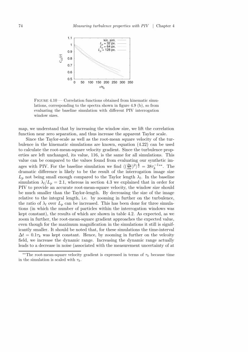
74 Measuring turbulence properties with PIV | Chapter 4
0.5
0.6
0.7
0.8
0.9
1
1.1
0 50 100 150 200 250 300 350
CLL
(r)
r/ηk
kin. sim.Lp = 32 px.Lp = 64 px.
Lp = 128 px.
Figure 4.10 — Correlation functions obtained from kinematic simu-lations, corresponding to the spectra shown in figure 4.9 (b), so fromevaluating the baseline simulation with different PIV interrogationwindow sizes.
map, we understand that by increasing the window size, we lift the correlationfunction near zero separation, and thus increase the apparent Taylor scale.
Since the Taylor-scale as well as the root-mean square velocity of the tur-bulence in the kinematic simulations are known, equation (4.22) can be usedto calculate the root-mean-square velocity gradient. Since the turbulence prop-erties are left unchanged, its value, 116, is the same for all simulations. Thisvalue can be compared to the values found from evaluating our synthetic im-
ages with PIV. For the baseline simulation we find 〈( ∂u∂x )2〉 1
2 = 38τ−1k
∗∗. Thedramatic difference is likely to be the result of the interrogation image sizeLp not being small enough compared to the Taylor length λl. In the baselinesimulation λl/Lp = 2.1, whereas in section 4.3 we explained that in order forPIV to provide an accurate root-mean-square velocity, the window size shouldbe much smaller than the Taylor-length. By decreasing the size of the imagerelative to the integral length, i.e. by zooming in further on the turbulence,the ratio of λl over Lp can be increased. This has been done for three simula-tions (in which the number of particles within the interrogation windows waskept constant), the results of which are shown in table 4.2. As expected, as wezoom in further, the root-mean-square gradient approaches the expected value,even though for the maximum magnification in the simulations it still is signif-icantly smaller. It should be noted that, for these simulations the time-interval∆t = 0.1τk was kept constant. Hence, by zooming in further on the velcoityfield, we increase the dynamic range. Increasing the dynamic range actuallyleads to a decrease in noise (associated with the measurement uncertainty of at
∗∗The root-mean-square velocity gradient is expressed in terms of τk because timein the simulation is scaled with τk.

4.4 | Applying PIV to simulated velocity fields 75
Table 4.2 — The measured root-mean-square velocity gradient as afunction of the ratio of λl, as obtained directly from the kinematicsimulation, over Lp.
λl
Lp〈(∂u
∂x)2〉 1
2 τk
2.1 433.0 494.9 68
best ≈ 0.1 pixel) and, consequently to a (small) decrease in measured velocitygradient fluctuation. The velocity fields generated with kinematic simulationsare incompressible and isotropic. Because of this, and as explained in section4.3, the longitudinal spectrum of velocity component u should be the same asthe longitudinal velocity spectrum of v, no matter how PIV influences the spec-trum. Similarly, the longitudinal as well as the transverse correlation functionsshould be independent of the direction. Figure 4.11 (a) shows both longitudinalspectra, Exx(kx) and Eyy(ky), for the baseline simulation. As expected thesespectra indeed are the same. The same rotation invariance was checked for thecorrelation functions in figure 4.11 (b), where we note that a small differenceis seen for the longitudinal correlations at large separations. We ascribe thisdifference to the finite sample size of the simulation.
As it involves derivatives, we do not expect the relation between the longi-
10-7
10-6
10-5
10-4
10-3
10-2
10-1
10-3 10-2 10-1
ELL
(k)
k/kη
Exx(kx)Eyy(ky)
(a)
0.2
0.4
0.6
0.8
1
0 50 100 150 200 250 300 350
C(r
)
r/ηk
Cxx(rx)Cyy(ry)Cxx(ry)Cyy(rx)
(b)
Figure 4.11 — (a) Longitudinal spectra in the x and y-direction ob-tained from PIV for the baseline simulation. (b) All four correlation-functions (two longitudinal and two transverse) for the same simula-tion.

76 Measuring turbulence properties with PIV | Chapter 4
0.2
0.4
0.6
0.8
1
0 50 100 150 200 250 300
CLL
(r)
r/ηk
directderived from CTT
(a)
0.2
0.4
0.6
0.8
1
0 50 100 150 200 250 300
CLL
(r)
r/ηk
directderived from CTT
(b)
Figure 4.12 — Comparison between the longitudinal correlationfunction and the corresponding longitudinal correlation function thatfollows from applying the relation for isotropic turbulence, equation(3.26), to the measured transverse correlation function: (a) in x-direction, ELL = Exx(kx) and ETT = Eyy(kx), (b) in y-direction,ELL = Eyy(ky) and ETT = Exx(ky).
tudinal and transverse correlation functions, equation (3.26), to hold. This isillustrated in figure 4.12 for the baseline simulation. In this case, derivativeswere simply done through the midpoint rule.
4.4.4 The influence of particle loss
In the kinematic simulations particle loss does occur. As was explained before,the most dramatic consequence of particle loss is the occurrence of spuriousvectors. This is illustrated in figures 4.13 and 4.14. These show results of asimulation in which the time between the images and the thickness of the lightsheet have been doubled relative to the baseline simulation. Hence in-planeparticle loss is doubled, but out-of-plane particle loss should remain unchanged.The maximum in-plane displacement for this simulation is roughly 8 pixels,which is one fourth of the interrogation window size. Figure 4.13 (a) showshistograms of both velocity components found with PIV, as well as a Gaussianfit to the u-component. At a first glance the histograms for u and v arevery similar, and as can be expected from a kinematic simulation, they areGaussian. However, not shown in this histogram is a single data point witha v-component of 45, which obviously is associated with a spurious vector. Aglobal mean filter, as suggested by Westerweel (1994), with a filter thresholdof 2 can obviously easily identify this. Figure 4.13 (b) shows the percentageof vectors that is removed by this filter as a function of the realisation. Inmost realisations no vectors are identified as spurious. However, in a singlerealisation as much as 0.45 % of vectors are spurious, which corresponds to

4.4 | Applying PIV to simulated velocity fields 77
10-5
10-4
10-3
10-2
10-1
100
-4 -2 0 2 4
(nor
mal
ised
) cou
nts
velocity
uv
gaussian fit
(a)
0 0.05 0.1
0.15 0.2
0.25 0.3
0.35 0.4
0.45
0 100 200 300 400 500
% s
purio
us v
ecto
rs
realisation
(b)
Figure 4.13 — (a) Histograms for both velocity components u and vas well as a Gaussian fit to the former. Note the logarithmic verticalscale. (b) Percentage of vectors identified as spurious based on aglobal filter that limits the normalised difference between any givenvector and the global mean of 2.
10-7
10-6
10-5
10-4
10-3
10-2
10-1
10-3 10-2 10-1
ELL
(k)
k/kη
uv
(a)
10-7
10-6
10-5
10-4
10-3
10-2
10-1
10-3 10-2 10-1
ELL
(k)
k/kη
uv
(b)
Figure 4.14 — (a) Longitudinal velocity spectra for both the u andv component of the velocity for velocity fields with a small number ofspurious vectors. (b) Corresponding spectra for the same fields withthe spurious vectors removed by a straightforward global mean filter.
12 vectors. In that particular realisation, within a small part of the image,the displacement exceeds 10 pixels. However, this small number of spuriousvectors has a dramatic influence on the spectrum. The reason is, of course,
that the used input spectrum, E(k) ∼ k− 5
3 , decreases rapidly with increasingk, which makes rare large wavenumber events, such as spurious vectors, standout clearly. This again emphasises the benefits of the spectral approach in thischapter. Figure 4.14 (a) shows both longitudinal spectra, Exx(kx) and Eyy(ky)

78 Measuring turbulence properties with PIV | Chapter 4
0
0.01
0.02
0.03
0.04
0.05
0.06
0 100 200 300 400 500
% s
purio
us v
ecto
rs
realisation
(a)
0 0.2 0.4 0.6 0.8
1 1.2 1.4 1.6 1.8
2
0 100 200 300 400 500
% s
purio
us v
ecto
rs
realisation
(b)
Figure 4.15 — Percentage of bad vectors as a function of the reali-sation for a sheet thickness (a) d = 6ηk and (b) d = 4ηk .
10-7
10-6
10-5
10-4
10-3
10-2
10-1
10-3 10-2 10-1
ELL
(k)
k/kη
d = 8 ηkd = 6 ηkd = 4 ηk
(a)
10-7
10-6
10-5
10-4
10-3
10-2
10-1
10-3 10-2 10-1
ELL
(k)
k/kη
d = 8 ηkd = 6 ηkd = 4 ηk
(b)
Figure 4.16 — Longitudinal velocity spectra for the u component ofthe velocity for simulations with different values for the thickness d ofthe light sheet. (a) For unfiltered velocity fields. (b) Correspondingspectra for the same fields with the spurious vectors removed by aglobal mean filter.
for unfiltered velocity fields. As we have seen before, the turbulence is isotropic.Hence the spectra should be the same. However, the spectra are very differentfor spatial frequencies k/kη above 2·10−2. This is due to the small percentage ofspurious vectors. The corresponding spectra for the filtered velocity fields shownin figure 4.14 (b) are practically identical, showing the success of the filter.Out-of plane particle loss has the same effect. This is demonstrated in figures4.15 and 4.16. These figures show the results of three different simulations:the baseline simulation, labeled d = 8ηk as well as two simulations with thinnerlight sheets with d = 6ηk and d = 4ηk. The particle density in these simulations

4.5 | Experiments 79
is set such that the number of particles within the sheet remains the same asin the baseline simulation. The time between the images is kept the same aswell. The main difference between these simulations is out-of-plane particleloss, which is increased as the sheet is made thinner. Figure 4.15 shows thepercentage of spurious vectors identified with a global mean filter with radius2urms for d = 6ηk and d = 4ηk. For the baseline simulation the percentageis 0. As expected, the percentage of bad vectors increases as the sheet getsthinner. Figure 4.16 (a) shows the longitudinal spectra for u for these threesimulations. The spectrum for the baseline simulation as well as the spectrumfor d = 6ηk are very similar, but the spectrum for the simulation with d = 4ηk
starts to deviate for frequencies k/kη above 2 · 10−2. Figure 4.16 (b) shows thecorresponding spectra for the velocity fields filtered with a global mean filter.Although as a result of this filter, the difference between the spectra becomessmaller, the spectrum with d = 4ηk still is clearly different.
A small number of spurious vectors can have a considerable effect on themeasured spectra. In a properly performed actual PIV experiment on average 1to 2 % of vectors per frame are spurious (Raffel et al., 1998; Westerweel, 1994).One would hope that the effect of such bad vectors were small. However, wehave seen that an even smaller number of bad vectors that occurs as a result ofparticle loss has a considerable effect on the measured spectra. For the spectrait is essential that they are effectively removed. Other statistics, such as meanand fluctuation velocities as well as correlation function fortunately are lessaffected. For the examples shown here a straightforward global mean filterseems to be fairly effective, as was already concluded by Westerweel (1994).However, our examples show that the criteria for particle loss by Keane &Adrian (1990, 1991) as well as the global mean filter have a clearly identifiableinfluence on the spectra.
4.5 Experiments
Our simultaneous PIV and surface slope measurements will be described indetail in chapter 8, following a description of the surface slope measurementtechnique and measurement results. Here we will compare PIV measurementsof grid-generated turbulence in our water channel with LDV measurements inorder to show how the averaging inherent to PIV is visible in the results of ourexperiments and to make sure that our PIV settings and set-up are reasonablysuited for measuring the turbulence. We will also take a look at isotropy in hor-izontal planes. Three different forcing conditions have been studied: active gridturbulence with protocols (25opt) and (25ran), and the static grid (25stat).The corresponding turbulence properties measured with LDV are listed in table3.2.
For the PIV experiments we use a dual pulsed Nd:YAG laser (SpectronLasers SL454, 200 mJ per pulse, 15 pulse pairs per second) to produce a light-

80 Measuring turbulence properties with PIV | Chapter 4
sheet in a horizontal plane below the surface. The flow is seeded with 100µm glass seeding particles (Dantec). A digital camera (Kodak ES 1.0, 8 Bit,1018 × 1008 pixels) is mounted below the water channel pointing upwards. Itimages an area of approximately 5.5 × 5.5 cm2 of the light sheet. The positioncalibration of PIV was done by recording an image of a plate with a patternof white dots against a black background, placed in the water channel insteadof the light sheet. Since the camera was placed relatively far from the plateand was carefully aligned such that its optical axis was perpendicular to theplate, a simple multiplication with a factor, based on the distance betweenthe points on the plate and in the camera image, is sufficient to perform theconversion from pixels to world coordinates. The integral scale of active-grid-generated turbulence found from our LDV measurements was approximately 8.5cm. The ratio between the image size and integral scale is approximately thesame in our experiments and in the kinematic simulations. We know from theLDV experiments that the root-mean-square velocity for active-grid-generatedturbulence is less than 3 cm/s. The 1/e width of the light sheet is approximately1 mm. In order to limit the influence of out-of plane particle loss, we havechosen very conservative values for the time interval between the paired imagesof ∆t = 1 ms for the active-grid-generated turbulence and ∆t = 3 ms forthe static grid, despite the criterion for out-of-plane particle loss by Keane &Adrian (1990, 1991), given in equation (4.2) allowing times between the imagesmore than twice as high. Indeed, the number of spurious vectors is very small(less than 0.5%). For these experiments we have used window shifting, withthe mean stream velocity corresponding to to 4 pixels in case of the active-grid-generated turbulence, whereas for the static grid generated turbulence itcorresponds to 12 pixels. A drawback of our conservative choice for ∆t is thatthe dynamic range is very limited, leading to a relatively high noise level inthe spectra, as we will see. Since spurious data have a very large effect on thespectra as well as on locally measured gradients, we decided that preventingspurious vectors was more important than the dynamic range. Similar to thekinematic simulations, for these PIV experiments we take 500 image pairs andthe images are evaluated with 32 × 32 pixel interrogation windows and 50 %overlap between neighbouring windows.
4.5.1 A comparison of PIV and LDV measurements
Unlike for the kinematic simulations, in our experiments we cannot prescribethe spectrum of the turbulence. However, as described in chapter 3, we do haveaccess to spectra and correlation functions measured by means of Laser-DopplerVelocimetry. Thus we can compare them to PIV measurements at the samelocations in the water-channel. The PIV light sheet is placed horizontally in thewater-channel. Thus, PIV provides the spanwise and streamwise components ofthe velocity, whereas the LDV system provides both the streamwise componentand the vertical component. Hence, we can only compare measurements of

4.5 | Experiments 81
the streamwise component of the velocity, v in our coordinate system. As wasexplained in chapter 3, with LDV we cannot measure spatial spectra directly,and have to resort to using Taylor’s frozen turbulence hypothesis to convertfrequency spectra into wavenumber spectra and, similarly, correlation functionsin time to correlations in space.
It should be noted that the Laser-Doppler and PIV measurements cannotbe performed simultaneously. Hence the LDV and PIV experiments were doneon different days. Furthermore, the experiments for the static-grid-generatedturbulence were done at a different time than those for the active grid, due tothe work involved in removing the active grid from the channel. However, theset-up and the settings used for PIV were kept the same. Table 4.3 shows mean
Table 4.3 — Comparison between mean and root-mean-square ve-locities measured with Laser-Doppler Velocimetry and Particle ImageVelocimetry for three forcing conditions.
v0 PIV v0 LDV vrms PIV vrms LDV(m/s) (m/s) (m/s) (m/s)
25opt 0.285 0.271 1.76·10−2 1.62·10−2
25ran 0.283 0.266 2.54·10−2 2.29·10−2
25stat 0.284 0.289 6.93·10−3 7.50·10−3
and root-mean-square velocities for three different types of forcing: the activegrid with protocols (25opt) and (25ran), and the static grid (25stat), at 2m behind the grid and at 10 cm below the surface. The table shows that themaximum difference in mean-stream velocities measured with PIV and LDV inthis set of experiments is less than 6%. The difference between the root-mean-square velocities is slightly larger, but still is less than 11%. In the kinematicsimulations we saw that PIV provides an accurate measurement of the root-mean-square velocities. Apparently the same applies to the experiments.
Figure 4.17 shows longitudinal spectra and correlation functions measuredwith LDV and the corresponding PIV measurements for the three conditionslisted in table 4.3. The spectra in figures (a), (b), and (c) illustrate the dra-matic difference in the range of scales that can be captured by PIV and LDV.By focusing on a relatively small area the large scales in the PIV spectra areunder-sampled. However, as we have seen before, in order to accurately mea-sure correlation functions at small separations we need a high spatial resolution.For a small range of wavenumbers, before the noise threshold is reached in bothspectra, the spectra are very similar. The noise level is reached at approxi-mately the same wavenumber, which can only be coincidental, since the causesfor noise are completely different in both techniques. The wavenumber where

82 Measuring turbulence properties with PIV | Chapter 4
10-5
10-4
10-3
10-2
10-1
100
101
10-1 100 101 102 103 104
ELL
/(vrm
s)2 (m
)
ky/2 π (m-1)
LDVPIV
(a)
0.4
0.5
0.6
0.7
0.8
0.9
1
1.1
0 0.01 0.02 0.03 0.04 0.05 0.06
CLL
ry (m)
LDVPIV
(b)
10-5
10-4
10-3
10-2
10-1
100
101
10-1 100 101 102 103 104
ELL
/(vrm
s)2 (m
)
ky/2 π (m-1)
LDVPIV
(c)
0.4
0.5
0.6
0.7
0.8
0.9
1
1.1
0 0.01 0.02 0.03 0.04 0.05 0.06
CLL
ry (m)
LDVPIV
(d)
10-5
10-4
10-3
10-2
10-1
100
101
10-1 100 101 102 103 104
ELL
/(vrm
s)2 (m
)
ky/2 π (m-1)
LDVPIV
(e)
0.1 0.2 0.3 0.4 0.5 0.6 0.7 0.8 0.9
1 1.1
0 0.01 0.02 0.03 0.04 0.05 0.06
CLL
ry (m)
LDVPIV
(f)
Figure 4.17 — Comparison of longitudinal spectra and correlationfunctions measured with LDV and PIV. (a) and (b): Active-grid-generated turbulence with protocol (25opt), (c) and (d) with protocol(25ran), and (e) and (f) static-grid-generated turbulence (25stat).
the noise level is reached, in both spectra, is still quite far below the rangewhere the inherent filtering in PIV starts to lead to a significant influence,

4.5 | Experiments 83
which obscures the influence of the spatial averaging. The similar comparisondone by Foucaut & Stanislas (2002) and Foucaut et al. (2004) with spectrameasured with hot-wire anememotry (HWA) showed a clear correspondencebetween the PIV measured spectrum and the HWA-spectrum multiplied withthe appropriate filter.
The correlation functions in figure 4.17 (b), (d) and (e) show a small peakat zero displacement that was not present in the results of the kinematic sim-ulations. This peak is the result of the high-frequency noise, which, of course,is perfectly correlated with itself. This peak was also observed in the corre-lation functions measured by Lecordier et al. (2001). This noise has only asmall influence on the root-mean-square velocity, but it has a far larger influ-ence on the measured fluctuation of the velocity gradients. In our experiments,velocity gradients are calculated using a simple mid-point rule. This derivativecalculation is very susceptible to noise in the velocity data. If we consider thatthe spectrum of the velocity gradient ∼ k2E(k), it is clear that the noise tailin the velocity spectrum is amplified in the derivative spectrum. In terms ofthe correlation function it can be understood as follows: if we consider equation(4.24), we see that as a consequence of the peak at zero displacement, the corre-lation at r = 2Lg = Lp is underestimated. This can be seen in table 4.4, wherethe root-mean-square velocity gradient is listed for the three different forcingconditions listed in table 4.3 alongside the corresponding values derived fromLDV measurements by means of equation (4.22). Because of this, the resultingvelocity gradient is overestimated, despite Lp being smaller than the correlationlength (λl/Lp = 8.4 for both (25opt) and (25ran), while due to a smaller λfor (25stat) the ratio is 5.3). According to Luff et al. (1999), who studied thevorticity field obtained from applying PIV to synthetic images of an Oseen-vortex, a dramatic improvement of the accuracy of the derivative calculationcan be achieved by using a Gaussian weighted averaging of the velocity field,before calculating the derivatives. Hence, in addition to the inherent filtering,in that case the measured velocity is further convolved with a Gaussian window
Table 4.4 — Fluctuation strength of the velocity gradient, 〈( ∂u∂x
)2〉 1
2 ,measured with PIV and derived from LDV, for turbulence with dif-ferent forcing.
LDV PIV PIV σLg
= 1.3 PIV σLg
= 3
25opt 1.4 s−1 3.2 s−1 2.4 s−1 1.3 s−1
25ran 2.0 s−1 3.8 s−1 2.6 s−1 1.6 s−1
25stat 1.1 s−1 1.4 s−1 1.0 s−1 0.67 s−1

84 Measuring turbulence properties with PIV | Chapter 4
function:
G(x) =1
σ
√2
πe−2( x
σ )2
, (4.41)
where σ is the width of the filter. According to Luff et al. (1999) the optimalvalue for σ = 3Lg, but for turbulence, where spatial resolution is a bigger issue,σ = 1.3Lg would be more appropriate. Of course, this Gaussian averaging isanother filter operation. It removes the noise tail from the velocity spectrumand the corresponding peak in the correlation function. This can be seen inthe spectra and corresponding correlation functions shown in figure 4.18. Table4.4 also lists the velocity fluctuations for the filtered PIV results. Clearly, thenumerical values for the filtered fields are closer to the values derived from PIV,and the correlation function also is closer to that measured with PIV, but notwithout a price, as can be seen in the spectra in 4.18 (a).
4.5.2 Isotropy in horizontal planes
In chapter 3 we have seen that, depending on the type of forcing, the isotropyof the turbulence in vertical planes (x =constant) changes. Since in our set-upPIV provides velocity fields in planes parallel to the surface, in similar fashionas for the kinematic simulations in the previous section, PIV allows us to studyisotropy in those planes. Figure 4.19 shows both longitudinal spectra as well asthe two longitudinal and transverse correlation functions for all three forcingconditions.
The two longitudinal spectra for active-grid-generated turbulence with pro-tocol (25opt) in figure 4.19 (a), as well as the two spectra for the static gridin figure 4.19 (e), are practically identical. Similarly, shown in figures (b) and(f), the longitudinal correlation functions for these two conditions overlap, as
10-16
10-14
10-12
10-10
10-8
10-6
10-4
101 102 103
ELL
(m2 s-1
)
ky/2 π (m-1)
no Gaussσ /Lg=1.3
σ/Lg=3
(a)
0.4
0.5
0.6
0.7
0.8
0.9
1
1.1
0 0.01 0.02 0.03 0.04 0.05 0.06
CLL
ry (m)
LDVno Gaussσ /Lg=1.3
σ/Lg=3
(b)
Figure 4.18 — Comparison of spectra and correlation functions forgrid-generated turbulence with protocol (25opt) without Gaussianfiltering and with Gaussian filtering with two different widths.

4.5 | Experiments 85
10-9
10-8
10-7
10-6
10-5
10-4
10-3 10-2 10-1 100
ELL
(k)
k/kη
Exx(kx)Eyy(ky)
(a)
0.2
0.4
0.6
0.8
1
0 50 100 150
C(r
)
r/ηk
Cxx(rx)Cyy(ry)Cxx(ry)Cyy(rx)
(b)
10-8
10-7
10-6
10-5
10-4
10-3 10-2 10-1 100
ELL
(k)
k/kη
Exx(kx)Eyy(ky)
(c)
0.2
0.4
0.6
0.8
1
0 50 100 150
C(r
)
r/ηk
Cxx(rx)Cyy(ry)Cxx(ry)Cyy(rx)
(d)
10-9
10-8
10-7
10-6
10-5
10-2 10-1
ELL
(k)
k/kη
Exx(kx)Eyy(ky)
(e)
0.2
0.4
0.6
0.8
1
0 50 100
C(r
)
r/ηk
Cxx(rx)Cyy(ry)Cxx(ry)Cyy(rx)
(f)
Figure 4.19 — Longitudinal spectra in the x and y-direction, as wellas all four correlation-functions (two longitudinal and two transverse)obtained from PIV. (a) and (b): Active-grid-generated turbulencewith protocol (25opt), (c) and (d) active-grid-generated turbulencewith protocol (25ran), and (e) and (f) static-grid-generated turbu-lence (25stat).

86 Measuring turbulence properties with PIV | Chapter 4
0.2
0.4
0.6
0.8
1
0 50 100 150
CLL
(r)
r/ηk
directderived from CTT
Figure 4.20 — Comparison of the transverse velocity correlationfunction measured with PIV with the transverse correlation functionderived from the relation for isotropic turbulence, equation (3.26), foractive-grid-generated turbulence with protocol (25ran).
0.2
0.4
0.6
0.8
1
0 50 100 150
CLL
(r)
r/ηk
directderived from CTT
(a)
0.2
0.4
0.6
0.8
1
0 50 100
CLL
(r)
r/ηk
directderived from CTT
(b)
Figure 4.21 — The isotropic relation, equation (3.26), applied to(a) active-grid-generated turbulence with protocol (25opt) and (b)static-grid-generated turbulence.
well as the transverse correlation functions. In chapter 3 we have already seenthat the turbulence for these conditions was nearly isotropic in vertical planes.Figure 4.19 now clearly shows that the same applies to isotropy in horizontalplanes. In chapter 3 it was also shown that the turbulence generated with pro-tocol (25ran) was less isotropic in vertical planes. The velocity spectra for thisprotocol in figure 4.19 (c) and the correlation functions in 4.19 (d) show that itis more anisotropic in horizontal planes as well. [b] Finally, we can take a lookat the validity of the relation between the longitudinal and transverse correla-tion functions for isotropic turbulence as obtained from PIV. In the previoussection we have seen that for our kinematic simulations, where λl/Lp = 2.1 it

4.6 | Conclusions 87
was not applicable.Figure 4.20 shows both the measured longitudinal correlation function as
well as the longitudinal correlation function derived from the isotropic relationfor active-grid-generated turbulence with protocol (25ran). However, some-what surprising in light of the failure of this approach for the kinematic simula-tions, corresponding images for the isotropic turbulence generated with protocol(25opt) and with the static grid in figure 4.21 show that the relation does hold.The most likely explanation for this is that in our measurements, the ratio ofλl/Lp was larger than in our kinematic simulations. In case of the active-grid-generated turbulence it was ≈ 9, and for the static grid it was somewhat smaller,but still ≈ 6 due to λl being smaller in that case.
4.6 Conclusions
In order to understand how PIV affects measured turbulence statistics, wehave introduced a simple model, which can be characterised as ‘spectrum in,spectrum out’. The great advantage of this approach is that experimental cir-cumstances can be easily tuned, including the spectral energy. A disadvantageis that higher order statistics cannot be modelled: a kinematic simulation pro-duces a Gaussian velocity field and only the second-order statistics are correct.The results of our model agree with the description of PIV in terms of a spa-tial average over the interrogation window by Keane & Adrian (1992). Wehave shown that this spatial averaging is the principal influence of PIV on thespectrum. It completely dominates over other artifacts of PIV such as particleloss, leading to spurious vectors. As predicted by Westerweel (1994), these canbe easily cured by simply removing them. This effect is clearly visible in outspectra.
Finally, we have compared experimental PIV results for grid-generated tur-bulence with those obtained from LDV. Despite the occurrence of considerablenoise, mostly due to a limited dynamic range, within the equally limited rangeof spatial scales, the PIV spectra were roughly comparable to those measuredwith LDV. By measuring correlation functions with PIV we were able to takea closer look at isotropy of the grid-generated turbulence in our set-up. Tur-bulence that was shown to be isotropic in vertical planes, by means of LDV,was shown to be isotropic in horizontal planes as well. We have demonstratedthat for these measurements it is vital that the interrogation window size ismuch smaller than the correlation length, i.e. the Taylor length-scale λ of theturbulence.
Due to the dramatic effect of the spatial averaging, PIV is not particularlysuited for measuring velocity spectra, unless digital cameras with far higherresolution become available. Even with a high resolution camera, the filteringinherent to PIV starts to influence the measurements even at larger scales thanthe size of the interrogation windows. Nonetheless, we have shown that un-

88 Measuring turbulence properties with PIV | Chapter 4
derstanding what PIV does to the spectrum is key to understanding how PIVaffects other measured properties. For instance, our description of the spatialaveraging explains why PIV can provide reasonable measurements of mean androot-mean-square velocities.
One way to overcome the inherent limitations of PIV is by means of so-calledhigh-resolution particle velocimetry (see Scarano & Riethmuller, 1999). This isa combination of PIV and Particle Tracking Velocimetry, in which the locationof the cross-correlation in a given interrogation window — corresponding toa spatial average of the displacement — is used as a first estimate for thedisplacement of individual particles. If this displacement is known, individualparticle images in the first frame in a pair can be matched to the correspondingparticle images in the next frame. In principle this allows a higher spatialresolution. However, the resolution in this case is no longer uniform across theimage, since it depends on the number of particle pairs that can be matched.

5
A statistical description of the surface
shape
Similar to turbulence, a description of the surface shape above sub-surfaceturbulence lends itself well to Fourier analysis. Unlike most descriptions ofturbulence, however, analysis of the free surface should involve both informa-tion in space and in time. This is essential, since waves can only be properlyidentified by looking at their behaviour in space and time, i.e. their dispersionrelation. In this chapter an overview of the various spectra and correlationfunctions of the surface shape is given. The spatial measurements also allow usto study isotropy. In this chapter we will derive relations between the spectraand correlation functions for isotropic surface deformations.
5.1 Basic definitions
In general, the height of the surface is a function of spatial coordinates x andy and of time t, so h(x, y, t). Similarly, the slopes hx = ∂h/∂x and hy = ∂h/∂yare functions of x, y, and t. For a scalar function η(x, y, t) we can define theauto-covariance function as:
Rη(rx, ry, τ) = 〈η(x + rx, y + ry, t + τ)η(x, y, t)〉, (5.1)
where 〈...〉 denotes an ensemble average∗ . The auto-covariance function is theensemble average over all possible values of t and x of the product of η in a point(x, y) at a time t with η in a different point (x + rx, y + ry) at a different timet + τ . Following Phillips (1980) the Fourier transform of an arbitrary functiong(t) in time is defined as:
g(ω) =1
2π
∫ ∞
−∞g(t)eiωtdt (5.2)
∗In many practical cases, instead of the covariance function R, we shall use itsnormalised equivalent: the correlation function Cη(rx, ry, τ) = Rη(rx, ry, τ)/(ηrms)
2.

90 A statistical description of the surface shape | Chapter 5
with inverse:
g(t) =
∫ ∞
−∞g(ω)e−iωtdω. (5.3)
More appropriately, since physically only ω ≥ 0 makes sense:
g(ω) =
0, ω < 01π
∫∞−∞ g(t)eiωtdt, ω ≥ 0.
(5.4)
Using similar definitions for Fourier transforms in space as in time† the Fouriertransform of an arbitrary function f(x) in one-dimensional space can be definedas:
f(k) =1
2π
∫ ∞
−∞f(x)e−ikxdx (5.5)
with inverse:
f(x) =
∫ ∞
−∞f(k)eikxdk (5.6)
in which k is the wavenumber. Using these definitions, the Fourier transformof η(x, y, z) in both space and time is:
η(k, ω) =1
(2π)3
∫∫∫η(x, t)e−i(k·x)+iωtdxdt (5.7)
in which (k · x) is the inner product of vector x = (x, y) and the wavenumbervector k = (kx, ky). The inverse of this is:
η(x, t) =
∫∫∫η(k, ω)ei(k·x)−iωtdkdω. (5.8)
Based on this, we can define the so-called wave spectrum of η(x, y, t): theFourier transform in space and time of the auto-covariance function Rη(rx, ry, τ):
Eη(k, ω) =1
(2π)3
∫∫∫Rη(rx, ry, τ)e−i(k·r)+iωτ drdτ, (5.9)
in which r = (rx, ry). This is directly related to the Fourier transform in spaceand time of η(x, y, t) itself through:
E(k, ω) = 〈|η(k, ω)|2〉. (5.10)
The auto-covariance in time is the cross-section of Rη(rx, ry, τ) for rx, ry = 0,so
Rη(0, 0, τ) = 〈η(t)η(t + τ)〉, (5.11)
†The difference in the sign of the exponent between the Fourier transform in spaceand that in time is to ensure that for a Fourier transform in both time and space, whichfollows, a wave with a positive value of kx travels in the positive x-direction

5.2 | Statistics of the slope at a point 91
which is symmetric relative to τ = 0. Its Fourier transform is the frequencyspectrum:
Eη(ω) =1
2π
∫Rη(0, 0, τ)eiωτ dτ. (5.12)
It can also be obtained more directly from a point measurement of η in time:
Eη(ω) = 〈|η(ω)|2〉 (5.13)
where η(ω) is the Fourier transform of η(t) measured in a point. The frequencyspectrum follows from the wave-spectrum through integration over wavenumberspace:
Eη(ω) =
∫ ∞
−∞
∫ ∞
−∞E(k, ω)dk (5.14)
=
∫ ∞
−∞Rη(0, 0, τ)eiωτ dτ
= 2
∫ ∞
0Rη(0, 0, τ) cos(ωτ)dτ.
To summarise: the frequency spectrum follows from the wave spectrum throughintegration over time and it is the Fourier transform in time of the auto-covariance function in time.
Similar to the frequency spectrum a spatial spectrum can be defined. Thisfollows from integration of the wave-spectrum over all possible ω:
Eη(k) =
∫ ∞
−∞E(k, ω)dω (5.15)
=
∫ ∞
−∞Rη(r, 0) exp(−i(k · r))dr
= 2
∫ ∞
0Rη(r, 0) cos(k · r)dr
in which Rη(r, 0) is the cross-section of the auto-covariance function in space:
Rη(rx, ry, 0) = 〈η(x + rx, y + ry, t)η(x, y, t)〉, (5.16)
which is symmetric relative to r = 0. So, the spatial spectrum is the integralover all frequencies of the wave-spectrum, and the Fourier transform in spaceof the auto-covariance function in space.
5.2 Statistics of the slope at a point
As was explained in chapter 3, measurements of turbulent flow are often pointmeasurements, in wind-tunnels usually with hot-wire anemometry and in this

92 A statistical description of the surface shape | Chapter 5
thesis with Laser Doppler Velocimetry. In a point measurement of the slope wemeasure hx(t) and hy(t) as a function of time. This enables calculation of thecorrelation functions for hx in time:
Rxx(t) = 〈hx(t0 + t)hx(t0)〉 (5.17)
and hy:Ryy(t) = 〈hy(t0 + t)hy(t0)〉 (5.18)
as well as the frequency spectrum in time for hx:
Exx(ω) =1
2π
∫Rxx(t)e
iωtdt = 〈|hx(ω)|2〉 (5.19)
and similarly for hy:
Eyy(ω) =1
2π
∫Ryy(t)e
iωtdt = 〈|hy(ω)|2〉. (5.20)
Unlike measurements of the turbulent velocity at a point as a function of time,however, these frequency spectra of the surface slope cannot easily be trans-formed into spatial spectra, since in the presence of free surface waves Taylor’shypothesis is not applicable. As a result of the Doppler effect, for waves thatare moving on top of a mean flow with a certain velocity v0, frequencies mea-sured in the non-moving frame are shifted relative to the frequencies in theframe that moves with the flow. This is illustrated in the following comparisonbetween a hypothetical measurement of the surface elevation in a coordinateframe that moves with the mean-stream velocity and a similar measurement ina fixed laboratory frame. The coordinate system used is shown in figure 5.1.If the actual shape of the surface in the coordinate system that moves withthe mean stream velocity is h(x, y, t), in the fixed laboratory frame we wouldmeasure hm(x, y, t), related to h(x, y, t) through a straightforward coordinatetransform:
hm(x, y, t) = h(x, y − v0t, t). (5.21)
xy v 0
Figure 5.1 — Top view of the coordinate system in the water-channel.

5.3 | Slope statistics in time and space 93
Its Fourier transform in time and space is given by:
hm(kx, ky, ω) =1
(2π)3
∫eiωt−ikxx−ikyy h(x, y − v0t, t) dx dy dt
=1
(2π)3
∫eiωt−ikxx−ikyy′−ikyv0t h(x, y′, t) dx dy′ dt
=1
(2π)3
∫ei(ω−v0ky)t−ikxx−ikyy′
h(x, y′, t) dx dy′ dt
= h(kx, ky , ω + v0ky). (5.22)
This means that for the wave spectrum the relation between the actual wavespectrum E and the measured spectrum Em is given by:
E(kx, ky, ω) = Em(kx, ky, ω − v0ky), (5.23)
which shows that wavenumber and frequency information are intertwined. Themeasured frequency is Doppler-shifted due to the convection. This situationis complicated further for waves, where the frequency itself is dependent onthe wavelength. A further complication can arise due to fluctuations in theadvection velocity due to sub-surface turbulence. As was shown before, thefrequency spectrum is the integral of the wave spectrum over k. As such, inthe measured frequency spectrum it is impossible to unravel the behaviour ofthe surface either in space or time. The frequency spectrum at any given fre-quency can contain contributions from waves with different wavenumbers. Forinstance, slowly traveling short waves can contribute to the same frequencyas fast traveling longer waves. Furthermore, the direction in which the wavestravel plays a role. Contributions to a single frequency can consist of a wave ofa certain wavelength traveling upstream with a certain phase-velocity, as wellas waves with a different wavelength traveling downstream with a different ve-locity. The solution to this problem is through a measurement of frequency andwavenumber in the direction y of the convection velocity. The actual frequencyspectrum of the surface scanned in the streamwise direction then follows from:
Eyy(ω) =
∫Em(0, ky , ω − kyv0)dky. (5.24)
5.3 Slope statistics in time and space
In the previous section we have seen that, especially in the case of surfacewaves, measurements of the slope both in time and space are essential forunderstanding the nature of the surface deformations. Our approach is tomeasure the slope along lines on the surface. From these measurements we cancalculate spectra of the surface slope in time and space. These can show whetherpart of the surface in fact consists of gravity-capillary waves. Furthermore, by

94 A statistical description of the surface shape | Chapter 5
measuring spatial correlation functions of the surface slope we can determinewhether or not the shape of the surface is isotropic.
5.3.1 Dispersive surface waves
For gravity-capillary waves the frequency of a wave is directly related to thewavenumber through the following well-known dispersion relation, the deriva-tion of which was shown in chapter 2:
ωd(k) =
√(gk +
k3σ
ρ
)tanh(kh0), (5.25)
in which h0 is the depth of the fluid (water), ρ is its density, σ is the surfacetension, g is the gravitational acceleration, and k is the length of wavenumbervector k. In most text-book examples, see for instance Kundu (1990), this re-lation is derived for one-dimensional waves, and even though in Kundu (1990)examples are given of two-dimensional wave-fields it is easy to overlook thatin real-world cases for a two-dimensional wavefield k has two components. Inwavenumber-frequency space, the dispersion relation represents a so-called dis-persion surface, also known as a dispersion shell (Senet et al., 2001), shown infigure 5.2 (a). For each wave-number vector k = (kx, ky) there is one matching
-1000-500
0 500
1000-1000-500
0 500
1000
0
500
1000
ωd (rad/s)
kx (rad/m) ky (rad/m)
ωd (rad/s)
(a)
kx (rad/m)
k y (r
ad/m
)
400 300 200 100
-1000 -500 0 500 1000-1000
-500
0
500
1000
(b)
Figure 5.2 — (a) The dispersion relation in wavenumber-frequencyspace. (b) Contours of ωd(k).
frequency ωd. Obviously the dispersion surface is cylindrically symmetric rela-tive to (kx, ky) = (0, 0) which is also evident from the contours of ωd(k) shownin figure 5.2 (b).
In our set-up, we have a mean stream velocity in the y-direction. For wavesmoving on top of a mean-stream velocity the dispersion-surface is deformed

5.3 | Slope statistics in time and space 95
-1000-500
0 500
1000-1000-500
0 500
1000
0
500
1000
ωd (rad/s)
kx (rad/m) ky (rad/m)
ωd (rad/s)
(a)
kx (rad/m)
k y (r
ad/m
)
700 600 500 400 300 200 100
0
-1000 -500 0 500 1000-1000
-500
0
500
1000
(b)
Figure 5.3 — The effect of a Doppler-shift due to a mean-streamvelocity of 0.25 m/s in y-direction. (a) The dispersion relation inwavenumber-frequency space. (b) Contours of ωd(k).
0
50
100
150
200
250
300
-1000 -500 0 500 1000
ωd
(rad
/s)
kx (rad/m)
(a)
-100
0
100
200
300
400
500
600
-1000 -500 0 500 1000
ωd
(rad
/s)
ky (rad/m)
(b)
Figure 5.4 — Cross-sections of the dispersion-surface with a mean-stream velocity of 0.25 m/s in the y direction: (a) cross-section forky = 0, (b) cross-section for kx = 0. The former remains symmetricbecause it is unaffected by the Doppler-shift. The latter is influencedby the Doppler-shift. Waves for which ky < 0 (upstream) appear tohave lower frequencies whereas waves for which ky > 0 (downstream)appear to have higher frequencies.
through the Doppler effect. For a mean-stream velocity v0 in the y-directionthe measured in non-moving frame of reference becomes:
ωd(k) =
√(gk +
k3σ
ρ
)tanh(kh0) + v0ky (5.26)
where v0ky is the contribution due to the Doppler-shift. Figure 5.3 (a) showsa graphical representation of the resulting dispersion surface with contours of

96 A statistical description of the surface shape | Chapter 5
ωd(k) shown in figure 5.3 (b). Obviously it is no longer cylindrically symmetric.The influence of the Doppler-shift is also clear from the cross-sections shown infigure 5.4. The cross-section in the kx-direction is unaffected by the Doppler-shift and remains symmetric relative to kx = 0, whereas the cross-section in ky
direction is Doppler-shifted, leading to waves with ky < 0 appearing to havelower frequencies than expected from the dispersion relation and waves withky > 0 appearing to have higher frequencies.
5.3.2 Spectra in time and space
For a field consisting only of linear gravity capillary waves the wave-spectrum isdirectly related to the wave-number spectrum through the dispersion relation:
E(ω,k) = E(k)δ(ω − ωd(k)), (5.27)
where the δ indicates the Dirac δ-function. In practice much of the energy in thewave spectrum of plane gravity-capillary waves is contained in wavenumbers andfrequencies around ω = ωd(k). This is actually applied in a maritime setting inorder to measure the near-surface current in the ocean. The current is derivedfrom a fit of the Doppler-shifted dispersion shell to the wave-spectrum of thesurface elevation in time and space, which is measured with a ship-mountedradar (Senet et al., 2001).
In our measurements we cannot access all of this information directly, sincewe do not have access to both spatial coordinates simultaneously. From ameasurement in the spanwise direction we can determine covariance functionsin time and space along the spanwise line:
Rxx(rx, 0, τ) = 〈hx(x + rx, y, t + τ)hx(x, y, t)〉 (5.28)
andRyy(rx, 0, τ) = 〈hy(x + rx, y, t + τ)hy(x, y, t)〉 (5.29)
and their two corresponding spectra:
Exx(kx, ω) =
∫ ∞
−∞Exx(kx, ky, ω)dky =
1
(2π)2
∫∫Rxx(rx, 0, ω)e−ikxrx+iωτdrxdτ
(5.30)and
Eyy(kx, ω) =
∫ ∞
−∞Eyy(kx, ky, ω)dky =
1
(2π)2
∫∫Ryy(rx, 0, ω)e−ikxrx+iωτ drxdτ.
(5.31)Similarly from streamwise measurements we can determine:
Rxx(0, ry, τ) = 〈hx(x, y + ry, t + τ)hx(x, y, t)〉 (5.32)

5.3 | Slope statistics in time and space 97
and:Ryy(0, ry , τ) = 〈hy(x, y + ry, t + τ)hy(x, y, t)〉. (5.33)
The corresponding spectra follow from the Fourier transforms or from inte-gration of the respective wave-spectra over kx and ky in similar fashion as inequations (5.30) and (5.31). Some of the properties of these spectra can alreadybe understood, without any prior knowledge of the exact nature of the surfacedeformations. The water channel is symmetric relative to x = 0, as well as thestatistical properties of the grid and the turbulent flow it generates. Hence,the covariance functions of the slope measured in x-direction are symmetricrelative to x = 0 and consequently the spanwise spectra are symmetric relativeto kx = 0. In streamwise direction the symmetry is broken by the mean-streamvelocity. Hence the time-space spectra in streamwise direction are not symmet-ric relative to ky = 0 and the time-space correlation functions are not symmeticrelative to y = 0. For gravity-capillary waves travelling on top of a mean-streamvelocity this is reflected in the dispersion shell and its cross-sections, previouslyshown in figure 5.3.
In addition to the one-dimensional time-space spectra we still have accessto the frequency spectra of the slopes, that can also be determined from pointmeasurements already given in equation (5.19) and equation (5.20). They arerelated to the four line spectra in time and space through integration over therespective component of k, so:
Exx(ω) =
∫ ∞
−∞Exx(kx, ω)dkx =
∫ ∞
−∞Exx(ky, ω)dky (5.34)
and
Eyy(ω) =
∫ ∞
−∞Eyy(kx, ω)dkx =
∫ ∞
−∞Eyy(ky, ω)dky. (5.35)
Finally, we can also calculate four one-dimensional spatial spectra. These arerelated to the spectra in time and space through integration over ω, so:
Exx(kx) =
∫ ∞
−∞Exx(kx, ω)dω (5.36)
and similarly Exx(ky), Eyy(kx), and Eyy(ky). They can also be calculated moredirectly from the measurements by Fourier transforming the slopes in space:
Exx(kx) = 〈|hx(kx)|2〉 (5.37)
and likewise Exx(ky), Eyy(kx), and Eyy(ky).As a consequence of measuring the slope as a function of space and time
along a line, the length of the wavenumber vector is unknown. This means thatsome of the drawbacks of point-measurements still remain. In the measuredspectra in time and space a range of wavenumbers k > kx can contribute to

98 A statistical description of the surface shape | Chapter 5
the spectrum in kx as and similarly wavenumbers k > ky can contribute to thespectrum at ky. Hence it is not immediately clear if and how the dispersionrelation will even be visible. Later we will see that the experimental results arealso complicated by the presence of other structures than waves on the surfaceand the fact that the sources of the waves are actually passing through themeasurement location.
5.3.3 Isotropy in the surface slopes
As we have seen in chapters 3 and 4, one of the standard ways to study isotropyin a turbulent flow is by comparing longitudinal and transverse correlation func-tions of the velocity. For incompressible three-dimensional isotropic turbulencea relation between the two can be derived (Pope, 2000):
CTT (r) = CLL(r) +1
2r
d
drCLL(r), (5.38)
which was previously used to study isotropy in our LDV turbulence measure-ments in section 3.3.3. Its equivalent expression for isotropic two-dimensionalincompressible turbulence is:
CTT (r) = CLL(r) + rd
drCLL(r). (5.39)
Unlike the velocity measurements in chapter 3, isotropy of the surface shapecan only be measured by means of spatial measurements. This is because of theinfluence of the Doppler-effect explained in section 5.2. We can find a relationbetween the transverse and longitudinal correlation functions for the surfaceslopes, similar to equation (5.39). The surface elevation can be described bya function h(x, y) ‡. The surface slope is obviously the gradient of the surfaceelevation:
hxex + hyey = ∇h. (5.40)
In our measurements the longitudinal covariance function RLL(r) correspondsto both 〈hy(x, y + r, t)hy(x, y, t)〉, which can be obtained from a measurementalong a streamwise line, and to 〈hx(x + r, y, t)hx(x, y, t)〉 from a spanwise mea-surement. The transverse covariance function RTT (r) corresponds to 〈hx(x, y+r, t)hx(x, y, t)〉 from a streamwise measurement and to 〈hx(x, y+r, t)hx(x, y, t)〉from a spanwise measurement. The correlation functions CLL and CTT (r) arethe covariance functions RLL(r) and RTT (r) divided by the root-mean-squareof the slope in any given direction, since for an isotropic surface this is inde-pendent of the direction in which it is measured. A way to check for isotropy
‡Of course h(x, y, t) is also a function of time. However, the dependence on timefor now is assumed implicitly since ensemble averages and temporal averages will betaken equivalent.

5.3 | Slope statistics in time and space 99
is to see whether the measured longitudinal correlation function is indeed in-dependent of the direction of the line along which we measure (spanwise orstreamwise).
A consequence of the fact that hx and hy are the gradient of scalar fieldh(x, y) is that they form a potential field:
∇ × (∇h) =∂
∂xhy −
∂
∂yhx = 0. (5.41)
We can use this to derive the relation between the transverse and longitudinalcorrelation functions for the surface slopes, via the surface slope covariancetensor, defined by:
R(r) =
(Rxx(r) Rxy(r)Ryx(r) Ryy(r)
)=
(〈hx(x)hx(x + r)〉 〈hx(x)hy(x + r)〉〈hy(x)hx(x + r)〉 〈hy(x)hy(x + r)〉
)
(5.42)Using equation (5.41) we find that:
∂
∂rxRxy(r) − ∂
∂ryRxx(r) =
∂
∂rx〈hx(x)hy(x + r)〉 − ∂
∂ry〈hx(x)hx(x + r)〉 =
〈hx(x)∂
∂rxhy(x + r)〉 − 〈hx(x)
∂
∂ryhx(x + r)〉 = 0 (5.43)
and similarly:∂
∂ryRyx(r) − ∂
∂rxRyy(r) = 0. (5.44)
In any isotropic field, we can write the covariance tensor as a combination ofrirj and δij , which defines the (scalar) longitudinal covariance function RLL(r)and the transverse covariance function RTT (r) (Pope, 2000):
Rij(r) = (RLL(r) − RTT (r))rirj
r2+ RTT (r)δij . (5.45)
The individual components of the tensor can now be written in terms of thesefunctions:
Rxx(r) = (RLL(r) − RTT (r))r2x
r2+ RTT (r)
Rxy(r) = (RLL(r) − RTT (r))rxry
r2
Ryx(r) = (RLL(r) − RTT (r))rxry
r2
Ryy(r) = (RLL(r) − RTT (r))r2y
r2+ RTT (r), (5.46)

100 A statistical description of the surface shape | Chapter 5
which serves to show that RLL indeed is the longitudinal covariance function.Substituting, for instance, r = (rx, 0) in Rxx leads to Rxx(rx, 0) = RLL(rx).Similarly, substituting r = (rx, 0) in Ryy leads to Ryy(rx, 0) = RTT (rx), thetransverse covariance function. Either equation (5.43) or (5.44) can now beused to find the relation between RLL(r) and RTT (r). We start by calculatingexplicitly the derivatives:
∂Rxy
∂rx=
rxry
r2
(dRLL
dr− dRTT
dr
)∂r
∂rx+ (RLL − RTT )
(∂
∂rx
rxry
r2
)=
=
(dRLL
dr− dRTT
dr
)r2xry
r3+ (RLL − RTT )
ry
r2
(1 − 2r2
x
r2
)(5.47)
and
∂Rxx
∂ry=
r2x
r2
(dRLL
dr− dRTT
dr
)∂r
∂ry+ (RLL − RTT )
(∂
∂rx
r2x
r2
)+
dRTT
dr
∂r
∂ry=
=
(dRLL
dr− dRTT
dr
)r2xry
r3− (RLL − RTT )
2ryr2x
r4+
dRTT
dr
ry
r. (5.48)
Substituting these expressions in equation (5.43) leads to:
(dRLL
dr− dRTT
dr
)r2xry
r3+ (RLL − RTT )
ry
r2
(1 − 2r2
x
r2
)
−(
dRLL
dr− dRTT
dr
)r2xry
r3+ (RLL − RTT )
2ryr2x
r4− dRTT
dr
ry
r= 0 (5.49)
which leads to the following relation between the transversal and longitudinalcovariance functions:
RLL = RTT + rd
drRTT . (5.50)
and since the root-mean-square of the slope is independent of the direction thedesired relation between the longitudinal and transverse correlation functionbecomes:
CLL = CTT + rd
drCTT . (5.51)
Performing similar substitutions in equation (5.44) obviously leads to the sameresult.
It is very interesting to compare this equation to the equivalent equation fortwo-dimensional isotropic turbulence given in equation (5.39). For the velocityfield, for which ∇ · u = 0, the occurrence of a difference in velocity compo-nents along a line, so in longitudinal direction, is hindered by incompressibility,whereas the transverse velocity component is unaffected. Hence, in an isotropicvelocity field the longitudinal correlation length is larger than that in transversedirection.

5.3 | Slope statistics in time and space 101
The effect of the free surface gradient field being irrotational is that theroles of the longitudinal and transverse correlation functions are reversed. Herethe occurrence of a difference in the transverse slope in two points on a lineis hindered by it being associated with twisting of the surface. A differencein longitudinal slope is associated with bending, as is illustrated in figure 5.5.Because of the different nature of these surface deformations, for an isotropicirrotational field the transverse correlation length is larger than the longitudinalcorrelation length.
h / x ( x 0 , y 0 )
h / x ( x 0 + x , y 0 )x
y
(a)
h / y ( x 0 + x , y 0 )
h / y ( x 0 , y 0 )
xy
(b)
Figure 5.5 — Illustration of the different type of deformation associ-ated with a difference in (a) the slope along a line (longitudinal) and(b) the slope perpendicular to a line (transverse).
Similar to the correlation functions, which were reduced from four functionsto only two, for isotropic surface waves the four one-dimensional wave spectraobtained from the measurements are reduced to two: the longitudinal andtransverse spectra. The longitudinal spectrum is the Fourier cosine transformof the longitudinal covariance function:
ELL(k) =2
π
∫ ∞
0RLL cos(kr)dr. (5.52)
For isotropic surface waves it corresponds to Exx(kx) and Eyy(ky) as defined inequations (5.36) and (5.37). Similarly the transverse spectrum corresponds toExx(ky) and Eyy(kx) and is the transform of the transverse covariance function:
ETT (k) =2
π
∫ ∞
0RTT cos(kr)dr (5.53)
By taking the Fourier cosine-transform of equation (5.51) we find the followingrelation between the longitudinal and transverse spectra:
ELL(k) = −kd
dkETT (k). (5.54)

102 A statistical description of the surface shape | Chapter 5
Similar to the relation between the correlation functions given in equation(5.51), this equation can, in principle, be used to check whether the surfaceshape is isotropic.
6
Measuring the slope of the free surface
From an experimental point of view, measuring the surface slope at a point asa function of time is relatively straightforward. Similar to, for instance, one-point hot-wire velocity measurements in a wind-tunnel, point measurements ofthe slope enable calculation of the frequency spectrum and the auto-correlationfunction of the slope in time. However, as shown in the previous chapter, thesespectra offer only a limited view of the nature of the surface deformations.Measurements of the surface in space and time are an absolute necessity. Inthis chapter, an existing technique for measuring the surface slope at a point isexplained. It forms the basis for a novel technique that allows measurement ofthe surface slope in space and time along a line. A comparison of experimentalresults obtained with both techniques allows us to test this new set-up.
6.1 Introduction
One of the first quantitative measurements of the surface gradient field involvedpictures of the sun glittering on the ocean surface (Cox & Munk, 1954). In ourwork we use the refraction of a focused laser beam by the surface to measurethe two components of the surface gradient at a point. By rapidly scanning theincident laser beam along a line, while at the same time sampling the location ofthe refracted laser beam, we measure the time-dependent gradient field along aline. For strongly curved surfaces, scanning techniques are unavoidable becausewhole-field measurements are thwarted by caustics and ambiguities. A similarscanning slope gauge has been described by Bock & Hara (1995) and Hara,Bock & Donelan (1997). Their device, which was successfully used for themeasurement of wind-driven waves, is suited for relatively low frequencies andlarge wavelengths (largest frequency ≈ 35 Hz, smallest wavelength ≈ 4 mm)and scans a circle on the surface. For our experiment a linear scan and a muchbetter space-time resolution was needed.

104 Measuring the slope of the free surface | Chapter 6
Jahne et al. (1994) review quantitative imaging techniques of ocean windwaves and conclude that scanning techniques for measuring the gradient fieldare most promising. It is good however, to put these techniques in the per-spective of whole field measurements. In this context, an often-used techniqueto look at spatial surface deformations is shadowgraphy (Settles, 2001). Inshadowgraphy images are formed as a result of the refraction of light passingthrough a transparent material of varying density. In the case of a free sur-face, this refraction occurs at the interface and the resulting image providesa view of the shape of the surface. For free-surface flows, shadowgraphy hasmainly been used to study the interaction of structures with the surface. Forinstance, Walker et al. (1995) has used shadowgraphy to study the interactionbetween a turbulent jet and a free surface. Sarpkaya & Suthon (1991), andGharib and Weigand (Weigand, 1996; Gharib, 1994; Gharib & Weigand, 1996)have used shadowgraphy to study vortex (dis)connection and the interactionbetween vortex rings and a free surface. However, obtaining quantitative infor-mation from shadowgraphy is often impossible and shadowgraphy is primarilya tool to qualitatively visualise the surface shape.
Zhang & Cox (1994) and Kurata et al. (1990) show that quantitative in-formation about the surface gradient field can be obtained from images of a(coloured) pattern that is either refracted in or reflected by the surface. Byreducing the scale of these patterns, Dalziel et al. (2000) developed a syntheticschlieren technique in which a randomly dotted pattern is refracted by the freesurface. Quantitative information about the surface shape is obtained by ap-plying a cross-correlation algorithm, similar to that used for Particle ImageVelocimetry, to a picture of the undisturbed pattern and a picture of the re-fracted pattern. All of these techniques are image-based. The actual image itselfprovides the (two-dimensional) spatial information. The spatial resolution ofthese techniques is limited by the density of the pattern used, or in case of thesynthetic schlieren technique by the minimum size of the interrogation windowsused for cross-correlating the images. The resolution in time in these techniquesis limited by the frame-rate of the camera. Increasing the frame-rate, throughthe use of a high-speed camera, has consequences for the measurement of lowfrequencies, since the duration of the measurement is limited by the maximumnumber of frames that can be stored.
In a geophysical setting, on an entirely different scale both in space (fromseveral meters up to kilometers) and in time (frequencies lower than 1 Hz ),several different techniques are used to measure wave-fields, including radar(altimeter) measurements from ships (Senet et al., 2001) or even from satellites(Forbes et al., 1993; Stammer, 1997) and photographs of sea surface glint takenfrom aircraft (Dugan & Piotrowski, 2003), as well as measurements from in situ
arrays of buoys and pressure transducers (Holland, 2001).

6.2 | Point measurements of the surface slope 105
6.2 Point measurements of the surface slope
The principle of the technique used to do point measurements of the slope isbased on refraction of a laser beam. Previously, this method was successfullyused to measure waves on the surface of a vertically oscillated fluid (Faradaywaves) (see Westra, Binks & van de Water, 2003).
The technique is illustrated in figure 6.1. A laser beam, originating from asmall 1 mW diode laser is sent perpendicularly through the transparent bot-tom of the water-channel and onwards to the surface, where it is refracted. Therefracted beam then proceeds onto a so-called Position Sensitive Device (PSD).This sensor is a dual lateral photo-diode, the layout of which is shown in fig-
d e f o r m e df r e e s u r f a c e
P o s i t i o n S e n s i n gD e v i c e ( P . S . D )
l a s e r b e a m
b e a md i s p l a c e m e n t
x - a x i sy - a x i s
Figure 6.1 — The principle of slope measurements in a point. Abeam is refracted by the surface. The beam’s displacement is mea-sured with a Position Sensitive Device.
ure 6.2. The sensor used in the point measurements measures 1 × 1 cm2 andwas manufactured by UDT sensors. It consists of a three-layer semi-conductingsilicon structure, biased with a bias voltage Vbias. Incident light on the photo-diode’s surface generates free electrons that change the local resistivity of thesemi-conducting material. As a result of this, the ratios of the cathode andanode currents Ic1,Ic2,Ia1, and Ia2, as indicated in figure 6.2, change and assuch their ratios can be used as a measure of the position of the illuminatedspot on the surface of the detector. For a square PSD of size L×L the positionsfollow from:
xPSD =Ia1 − Ia2
2IphL (6.1)
and
yPSD =Ic1 − Ic2
2IphL, (6.2)

106 Measuring the slope of the free surface | Chapter 6
V b i a s
I c 2I c 1
I a 1
I a 2
x P S Dy P S D
pin
i n c i d e n tl i g h t
I p h
Figure 6.2 — Layout of a Position Sensitive Detector.
in which Iph is the total photo-current. Because of these ratios, the sensor isinsensitive to the intensity of the laser spot, with the position signal reflectingthe centre of mass of the laser spot. We emphasize that this only works if thefour photocurrents can be measured exactly simultaneously and the transportof the photo charges across the sensor is instantaneous. The currents are mea-sured and the various subtractions and divisions are performed in an analoguePhillips PSD processor board (type CTR 531.91.0017). This provides two out-put voltages Vx and Vy, which correspond to the positions xPSD and yPSD. Theresponse speed of the measurement technique in this configuration is limitedby the electronic circuitry in the processor board, but generally a PSD offersa far better resolution in time than a pixel-based detector such as a CCD orCMOS. The spatial resolution of the PSD is limited by both shot noise andthermal noise of the resistive layer. The linearity of the response is primarilydependent on the quality of the substrate layers of the PSD. In practice we usea linear transformation from voltages to positions, based on a separate calibra-tion of the PSD. The PSD-Voltages are digitised for processing and storage ona computer by means of a PhyDAS PARSAM (PARallel SAMpling) unit, witha sample frequency of 30kHz.
The free surface gradient in x and y-directions can be calculated from thedisplacements δx, δy of the spot on the PSD surface from:
∂h
∂x=
−δx
H − nw
√H2 + (δx)2 + (δy)2
and∂h
∂y=
−δy
H − nw
√H2 + (δx)2 + (δy)2
.
(6.3)The displacements δx, δy are calculated by subtracting the average positionof the spot taken over the entire measurement time from the instantaneous

6.3 | Measuring the slope in space and time 107
position,δx = xPSD − 〈xPSD〉, δy = yPSD − 〈yPSD〉, (6.4)
where xPSD and yPSD are the instantaneous positions and 〈xPSD〉 and 〈yPSD〉are the corresponding averages.
This method is based on the notion that on average a turbulent surface ishorizontal. Since the right-hand-side of equations (6.3) depends non-linearlyon δx and δy, a zero average of ∂h/∂x and ∂h/∂y is not the same as a zeroaverage of δx and δy, but we found the error to be negligible. Calibrationrequires a measurement of the height H of the PSD above the (undisturbed)surface and the conversion of measured PSD voltages to position, which wascalibrated in a separate experiment. All other information needed to convertmeasured voltages to surface slopes follow from the measured time series. Thismethod is straightforward, sensitive, and linear. However, it only provides thetime-dependence of the surface slope in a point. For a surface that is advectedby the mean flow, this information is ambiguous as temporal fluctuations mayalso be caused by spatial fluctuation which are swept past the measurementlocation. We next describe the extension of this technique to measurement ofthe time-dependent gradient field along a line.
6.3 Measuring the slope in space and time
6.3.1 Set-up for slope measurements along a line
As already mentioned, in order to measure the surface slope in space and timewe have chosen to measure the slope along a line. The technique used for thisis an extension of the existing technique used for point measurements. Thenew set-up is illustrated in figure 6.3. Instead of being aimed at a single pointof the surface, now the laser beam is swiveled back and forth by a rapidlyoscillating mirror (an Electro Optical Products Corp. SC-30 resonant scanningmirror). Changes in the signal that occur more rapidly than those due to theoscillating motion are interpreted as spatial variations of the surface slope alongthe line. A drawback of this technique compared to image-based surface slopemeasurements is that it only provides one spatial coordinate. However, it doesoffer a much higher resolution in time as well as a higher spatial resolution alongthe line. Obviously, it is impossible to measure structures on the surface thatare actually smaller than the size of the light spot on the surface, which is whythe laser beam is passed through a lens that focuses it on the surface. As willbe explained in more detail shortly, the length of the line on the surface is toolarge to allow the refracted beam to be projected directly onto the PSD. Hence,after passing through the free surface the refracted beam falls onto a plate ofhigh quality frosted glass. This leads to an illuminated dot being visible on thetop side of the frosted glass, at the location where the beam hits it. This spotis projected onto the PSD. By sampling the PSD signals at a higher rate fs

108 Measuring the slope of the free surface | Chapter 6
P o s i t i o n S e n s i t i v e D e v i c e( P S D )
i m a g i n g l e n s e s
f r o s t e d g l a s s
H e - N e l a s e r
o s c i l l a t i n g m i r r o r
c h a n n e l s e c t i o n
s c a n n i n g b e a m
f o c u s i n g l e n s
y xHL s
L g
Figure 6.3 — Set-up for measuring the surface slope along a line.
than the oscillation frequency fm of the mirror, the position of the spot on thePSD is measured multiple times during each mirror period, thereby providingthe slope in multiple points on the line. In our case we can measure the slopein 152 points along a 5 cm line.
6.3.2 Synchronisation
The electronics that control the oscillating mirror also provide a periodic squarewave voltage, at the frequency at which the mirror oscillates. This signal servesas a triggering signal for a purpose-built electronic timing unit, which in turndelivers a predetermined number n of trigger signals at a fixed frequency to theADC. This means that the positions on the line at which the PSD voltages aresampled are fixed in time relative to the phase of the mirror. This is illustratedin figure 6.4. Let us call p, with p = 1, ..., n, the index of a sample in eachblock of n samples and q, q = 1, 2, ... the index of a block. Then the index p

6.3 | Measuring the slope in space and time 109
m i r r o r p o s i t i o n
r e f e r e n c e s i g n a l
t r i g g e r s i g n a l
t i m e
f m = 1 . 9 6 k H z
f s = 3 0 0 k H z
Figure 6.4 — Synchronisation of the surface gradient scanner. Themirror control unit provides a block signal with the same frequencyas the mirror movement (fm =1.96 kHz). This triggers a timing unitwhich sends blocks of 152 trigger signals at sample frequency fs =300kHz to the ADC. Each line sample is one cycle of the mirror, in whicheach point on the line is visited twice. The unit has further provisionsto synchronize the line scan to a particle image velocimetry system.
corresponds to a point on the scanned line, while q is an index, fq = q/fm,corresponding to the time at which the line was measured. We will now showhow the samples define the surface gradient hx(x, y, t) and hy(x, y, t).
Let us assume that the laser beam is scanned in the x-direction. Afterrefraction through the surface the signal of the PSD contains two components:V x and V y corresponding to the deflections of the laser beam in the x- andy- directions, respectively. The samples V x
p,q include two contributions: a largecontribution due to the beam being swiveled back and forth by the oscillatingmirror and a smaller contribution resulting from the actual changes in slopein the points of the line. The other sampled voltage, V y
p,q, only contains acontribution from the changes in slope∗. Provided that the imaging by thissystem is linear, the position xg
p,q of the spot on the glass and the voltage V xp,q
from the PSD are related through:
V xp,q = Axg
q,p + Bx, (6.5)
in which A is a proportionality constant that is the same for deflections in x- andy directions and Bx is an offset that depends on the component of the measureddeflection. These constants can be easily found from the measurement. Sinceon average the surface is flat, the time (q) average of the measured voltage V x
∗In practice one can expect there to be some misalignment, leading to a smallcontribution due to the scanning also being present in V y. However, this has no effecton the measurement of the slope itself, since the average trace of the spot in the surfaceis subtracted, as will be explained later.

110 Measuring the slope of the free surface | Chapter 6
isV x
p = 〈V xp,q〉q = Axg
p + Bx, (6.6)
where xgp are the positions corresponding to the trace of the line on the glass if
the surface were flat. Thus the peak-to-peak amplitude V xa of V x
p correspondsto the length of the line on the glass. The proportionality constant A nowfollows from dividing the peak-to-peak amplitude V x
a by the actual physicallength of the line on the glass, Lg,:
A =V x
a
Lg. (6.7)
Of course, since the relation between the surface slope and the laser beamdeflection is non-linear, this procedure is not strictly correct. However, we haveascertained that, similar to the point measurements, the error is negligible. Theconstants that determine the coordinates (xw
p , ywp ) on the actual water surface
are determined analogously to those on the glass; for example the correspondingproportionality constant would be V x
a /Ls, in which Ls is the length of the lineon the water surface.
Finally, the equations for the measured surface gradient field are similar tothose of the point measurement, equation (6.3):
∂h(x, y, t)
∂x
∣∣∣∣x=xw
p ,y=ywp ,t=q/fm
=−δxp,q
H − nw
√H2 + (δxp,q)2 + (δyp,q)2
(6.8)
and
∂h(x, y, t)
∂y
∣∣∣∣x=xw
p ,y=ywp ,t=q/fm
=−δyp,q
H − nw
√H2 + (δxp,q)2 + (δyp,q)2
(6.9)
in which H is the height of the glass above the undisturbed surface and δxp,q
and δyp,q are displacements of the spot on the glass with respect to the tracedaveraged curve:
δxp,q = xp,q − xp =V x
p,q − V xp
A(6.10)
and:
δyp,q = yp,q − yp =V y
p,q − V yp
A. (6.11)
Obviously, for a correct assignment of the gradient field it is crucial to carefullykeep track of the various signs of displacements and digitised voltages.
Calibration of this slope measurement technique requires only straightfor-ward measurements of three lengths, also indicated in figure 6.3 :
1. The height of the glass above the surface H is needed in order to calculatethe slopes from the displacement on the frosted glass from equations (6.8)and (6.9).
6.3 | Measuring the slope in space and time 111
2. The length of the scan-line Lg on the glass is needed to find the propor-tionality constant A in equation (6.7). If it is known, the actual positionson the glass can be calculated.
3. The length of the line on the surface Ls is required in order to calculatethe actual position of each point on the line on the water surface.
It should be noted that due to the use of a swiveling beam the beam crossesboth the bottom of the channel as well the surface at a small angle. The effectof this is almost completely removed by subtracting the averages. Its residualeffect may be a small bias, which may become somewhat more pronounced forthe extreme points on the line. In theory it is possible to correct for this. Theexact position where the light beam falls onto the frosted glass depends on theslope at the surface as well as on the elevation of the surface. However, in ourset-up changes of the position on the glass relative to the average position areinterpreted as resulting from a change of the slope at the surface. As with thepoint measurements, the influence of changes in the elevation of the surface isneglected, since their effect is very small compared to the effect of a change inthe slope, especially since the anticipated changes in the elevation (at most afew mm) are tiny compared to H (30 cm).
The use of a plate of frosted glass is an unfortunate necessity. Directlyprojecting the line onto the PSD is not possible, despite the use of a larger 2× 2 cm2 PSD for these measurements. The reason is that the optics neededto directly project the refracted laser beam onto the PSD is subject to incom-patible requirements. In order to accommodate the largest possible surfacegradient (Sm = O(0.3)) in our experiments, the lens must be placed as near tothe surface as possible, with its focal length F as the minimal distance. Then,if the length of the scanned line is Ls, the diameter of the lens should at leastbe 2 F Sm + L. Although lenses with Sm = 0.3 do exist, they are difficult tomanufacture and their imaging is far from ideal. The problem is that in directimaging of the refracted laser beam, angle and position are coupled. Further,with the surface in the focal plane of the lens, the position on the PSD woulddepend on both the angle and the position at which the laser beam enters thelens. However, the surface gradient itself is only reflected in the angle of thelaser beam. Unravelling these contributions by calibrating would be exceed-ingly difficult. The major benefit of using the frosted glass is that now angleand the position become decoupled. A drawback of this method is, however, alarge loss of light intensity and the introduction of speckles in the light spot.To optimise the light intensity the laser spot on the frosted glass is imagedonto the PSD detector surface by using two very strong large-diameter lenses.To further increase the intensity of the light on the PSD a relatively powerful(approx. 30 mW) He-Ne laser was used.
In order to increase the response speed of the measurement technique, theprocessor board we used for the point measurements, has been replaced by a

112 Measuring the slope of the free surface | Chapter 6
purpose-built new electronic circuit, which amplifies the four PSD currents andseparately converts them to voltages. These four voltages are then individuallysampled by means of a four-channel parallel Analogue to Digital converter (Na-tional Instruments Ni-DAQ 6115) at the sample frequency of 300 kHz. Insteadof measuring voltages V x and V y, the (relative) positions on the PSD are nowactually calculated in post-processing by means of equations (6.1) and (6.2).The time response of the PSD itself now determines the smallest changes thesurface slope along the line that we can find with our scan technique. Sincethe position signal of the light spot depends on intensity ratios, the positionsignal is insensitive to intensity fluctuations of the refracted laser beam. Inour experiment intensity fluctuations are caused by scattering off particles inthe flow (used in PIV experiments) and by speckles of the frosted glass screen.However, the intensity normalisation can only work if all currents are measuredsimultaneously. The problem is that photo-charges in the PSD have a finite ve-locity, set by the capacity of the light-sensitive layer. The propagation delay is afew µs, which in our case corresponds to the used sampling frequency (fs =300kHz). At those frequencies intensity variations are seen as position variations.Without a faster PSD, no further improvement of the signal-to-noise ratio ispossible.
The positions xp on the scan line are sampled sinusoidally: the points crowdnear the extremes of the sweep, and they are sampled fastest near the zero-crossings of the sweep. We expect that a further effect of the propagationdelays of the photo-charges is that samples of the surface slope near the zero-crossings will have different properties from those at the extremes of xp. Wewill assess this possible source of inhomogeneity below.
The overall set-up is more complicated than the set-up used for point mea-surements. Moving the optical system along the water channel is far moredifficult. Because of this we have chosen to place the set-up at a fixed positiontwo meters downstream from the turbulence generating grid, not coincidentlythe same position as where we performed the Laser-Doppler measurements ofthe turbulence properties described in chapter 3.
6.3.3 Data processing
The data processing is done with a series of computer programmes. In orderto obtain surface gradient information from the stored data, the file (typicallyseveral GBytes in size) is first unravelled in samples V x
p,q and V yp,q. If, for
example, the laser beam is scanned in the x-direction sample V xp,q contains the
relevant information about the scan. Since perfect synchronisation is crucialfor this method, the relative phase of the samples V x
p,q is monitored constantlythrough computing the auto-correlation function of V x
p,q. Phase drifts mayoccur due to temperature changes of the resonant mirror. A measurement ofthe phase reveals that the relative phase-shift of the mirror is O(10−3) over theduration of the longest measurement, which is negligible. Next, the coordinates

6.3 | Measuring the slope in space and time 113
(xp, yp), p = 1, .., n are computed from phase-sensitive averages of V x and V y.Finally the surface gradients hx(xp, yp, tq) and hy(xp, yp, tq) are computed.
The key questions are about the homogeneity of the measurement techniquealong the scan line and its spectral response. Several useful statistical quantitiescan be computed from the measured gradient field and may be used to answerthese questions. In the case of homogeneous turbulence, the normalized space-time correlation function
Rxx(xi, xj , τ) =〈hx(xi, t + τ) hx(xj , t)〉
〈h2x(xi, t)〉1/2 〈h2
x(xj , t)〉1/2(6.12)
and similarly Ryy, Rxy, depends only on the separation r = xi − xj , and noton the individual coordinates xi, xj . As different points xi on the scan line aretraversed with different velocities of the swiveling laser beam, the question iswhether this property holds for the measured correlation function. We approachthe correlation function through the cross-spectral density
Cxx(xi, xj , ω) =⟨hx(xi, ω) h∗
x(xj , ω)⟩
. (6.13)
where hx is the temporal Fourier transform of hx. The advantage of the cross-spectral density is that it involves Fourier transforms in the homogeneous timedirection, but it retains the dependence on the spatial coordinates. In order to
improve the statistical accuracy of Cxx we perform a frequency average∫
K(ω, ω′) Cxx(xi, xj , ω′) dω′, (6.14)
where the kernel K(ω, ω′) is a tent-function centred on ω, and whose width inω′ increases exponentially with increasing ω. Such an average is most appro-priate for energy spectra that have an algebraic dependence on the frequency.From the cross-spectral density we can compute the frequency spectrum at each
spatial point, Exx(xi, ω) = Cxx(xi, xi, ω). Finally, the covariance function Eq.6.12 is only a Fourier transform away
Rxx(xi, xj , τ) =<∫∞0 eiωτ Cxx(xi, xi, ω) dω
(∫∞0 cos(ωτ )Cxx(xi, xi, ω) dω
∫∞0 cos(ωτ )Cxx(xj, xj , ω) dω
)1/2,
(6.15)where < denotes the real part. We will demonstrate that to good approximationthe covariance function R only depends on the separation of the points, andnot on their individual coordinates:
rk = xi − xj , k = 1, . . . , n(n − 1)/2. (6.16)
However, significant errors exist. Clearly, computing the space-time correlationfunction of the surface gradient by means of the cross-spectral density is the

114 Measuring the slope of the free surface | Chapter 6
only practical option, as direct computation in the time domain would takeprohibitively long.
Direct computation of the spectrum of the surface gradient, h(kx, ω), ispossible by resampling the coordinates along the line, xp in our example, andthen performing a fast-Fourier transform both in space and time. The surfacefields hx(x, y, t) and hy(x, y, t) themselves are stored for further processing, forexample in order to assess the validity of Taylor’s frozen turbulence hypothe-sis for the surface. Although we only have information about a single spatialdimension (and time), the gradient field signals allow us to measure statisti-cal quantities of a turbulent surface which, to our knowledge, have not beenmeasured before.
6.4 Assessment of the surface scanning method
Before proceeding with the experimental results for the surface above grid-generated turbulence as well as a first physical interpretation, we will first takea look at a number of tests of the surface scan technique. We need to testwhether the imaging of the scan line through the frosted glass, the lenses andthe PSD is linear, since this is one of the assumptions made in the previoussection. Further tests revolve around the frequency response of the PSD. ThePSD needs to be able to follow changes in the position of the spot on its surfacefaster than the mirror frequency (approximately 2 kHz), since these are to beinterpreted as spatial variations. Our first interest will be the average positionsxw
p and ywp .
0 50 100 150-.04
-.02
0
0.02
0.04
p
x p(m
)
-.04 -.02 0 0.02 0.04y p (m)
(a) (b)
Figure 6.5 — Linearity of the imaging by the surface scan set-up.(a) A harmonic scan in streamwise direction. Full line the averagecoordinate yw
p computed for a turbulent surface. Because of the har-monic scan, yw
p should ideally be ∝ sin(2πpfm/fs + ϕ). Dashed line:A sin(2πpfm/fs + ϕ), with amplitude A set to the amplitude of yw
p
and measured phase ϕ = 1.088 π.
The oscillating mirror swivels the laser beam approximately harmonicallyin time. Hence for a scan line in x-direction the average position of the spot onthe PSD surface should depend on p as sin(2π p/fs + ϕ). This is very nearly

6.4 | Assessment of the surface scanning method 115
so, as is illustrated in Figure 6.5 (a). We conclude that non-linearity effects inthe imaging are small†. Figure 6.5 (b) shows xp versus yp, i.e. the trace of thesurface scan for both a spanwise and streamwise scan. This figure shows thatthe adjacent points in a scan form an approximately straight line, as intended.Furthermore, Figure 6.5 (b) shows that the PSD and its associated electronicscan follow the illuminated spot on the surface, even though it moves back andforth at almost 2 kHz. Any phase difference between the measured x- and y-deflections would have resulted in a Lissajous-loop.
The alignment of the set-up is relatively straightforward. The hardest partis aligning the direction of the scan line. Changing the direction of the scan line,which is very useful when studying the isotropy of the surface gradient field,involves moving the oscillating mirror, the focusing lens, and several mirrors.Yet, it is possible to properly align the scan-line in spanwise direction as wellas aligning it in a practically perpendicular, i.e. in streamwise direction, atessentially the same location in the channel, as can also be seen from Figure6.5 (b). A first impression of the detector homogeneity can be obtained fromthe probability distribution function (PDF) of surface gradients on a turbulentchannel flow. The variation of the PDF along the scanned line is shown inFig. 6.6. In this experiment, the scanned line points in the x-direction. As thelength Ls of the scanned line is 5 cm, which is much smaller than the widthof the channel (30 cm), we can assume that the turbulence is homogeneous.The measured PDF is very nearly independent of the position on the scanningline, but a small systematic effect for the rare large |dh/dx| events can be seen.Figure 6.6 also demonstrates that the gradient fluctuations are very nearlyGaussian. A quite similar result was obtained for scans in the streamwise(y) direction. In this direction the grid-generated turbulence decays, but thevariation of its statistical properties over the length of the scan line is negligibleas Ls = 5 cm is small compared to the distance (2 m) of the scanner behindthe turbulence generating grid.
In order to see how scanning affects the signal-to-noise ratio, we now com-pare frequency spectra of the surface slope at a point measured with the surfacescanning technique to spectra measured under the same experimental conditionswith an actual point-measurement. In the last case, the surface slope followsdirectly from the registered signal, while in the former case is wrapped in thespatial scan in the first case. The frequency spectrum obtained from the linescan in this case is actually the frequency spectrum in one of the 152 points onthe 5 cm long line. Results obtained with both techniques for static grid gen-erated turbulence, are shown in Figure 6.7 (a). Up to a frequency of 50 Hz thespectra are very similar, despite the different PSD signal processing electronics,different PSDs, the very different optical systems as well as the difference in
†The quality of the harmonic fit is not only due to the linearity of the imaging.Deviations of the harmonic dependence and curved scan lines can also occur due tothe axis of rotation of the mirror not being parallel to the mirror surface.

116 Measuring the slope of the free surface | Chapter 6
-.05 0 0.0510 -4
10 -3
10 -2
0.1
1
10
-.02
0
0.02
dh / dx
x (m)
-.05 0 0.0510 -4
10 -3
10 -2
0.1
1
10
dh / dx
(a)
(b)
Figure 6.6 — (a) Probability density function (PDF) of surface gra-dients dh/dx as a function of the position x on the scan line. Thescan line is oriented perpendicularly to the mean flow velocity in thechannel. (b) Full line: PDF averaged over x, dashed line: Gaussianfit. The turbulence with mean velocity U = 0.25 m/s is generatedwith the active grid.
calibration methods. Above 50 Hz the spectra from the scan are drowned innoise, while the point spectra continue up to roughly 1 kHz. This is not due toa limitation in frequency response, however, since we have already seen that thePSD and its electronics can follow the spot moving back and forth at almost2 kHz. The difference between the spectra is due to the lower signal-to-noise

6.4 | Assessment of the surface scanning method 117
0.1 1 10 10 2 10 3 10 410 -12
10 -10
10 -8
10 -6
10 -4
Exx
, Eyy
(s)
0.1 1 10 10 2 10 3 10 4
(a) (b)
f (Hz)
Figure 6.7 — Comparison of frequency spectra of the slope measuredwith point-measurements and derived from line measurements. Theturbulence with mean-stream velocity of U = 0.28 m/s was generatedwith a static grid. (a) Eyy, point spectra of the streamwise slope. (b)Exx, point spectra of the spanwise slope. Full lines: using a pointmeasurement, dashed lines: spectra at one of the points of a linemeasurement.
1 10 10 2 10 310 -9
10 -8
10 -7
10 -6
10 -5
10 -4
Exx
, Eyy
(s)
1 10 10 2 10 3
(a) (b)
f (Hz)
Figure 6.8 — (a) Point spectrum of the spanwise slope, Exx, fromboth a spanwise and streamwise scan. (b) Point spectrum of thestreamwise slope, Eyy, from both a spanwise and streamwise scan.The turbulence with mean velocity U = 0.25 m/s was generated usingthe active grid.
ratio as a result of the spot’s relatively low light intensity, and the presence ofthe ground glass screen. Still, the spectrum from the scan covers several ordersof magnitude.
A comparison of spectra measured in a spanwise scan with those measuredwith the scan line in the streamwise direction can potentially reveal limitationsin the detector’s frequency response. The position signal in the scan directionchanges much more rapidly than that in the perpendicular direction. Hence,limitations in the frequency response of the PSD are most likely to affect themeasurement of the slope in the scan direction. However, the frequency spec-

118 Measuring the slope of the free surface | Chapter 6
1 10 10 2
10 -8
10 -7
10 -6
10 -5
-.02-.01
00.01
0.02
f (Hz)
E(f)
(s)
x (m)
Figure 6.9 — Point frequency spectra as a function of the positionof the point x on the scan line. The depression in the centre of thescan line signifies a reduction of the gradient-detector sensitivity.
trum of the slope at a point on a surface scan line should be completely inde-pendent from the direction of that line. However, if the frequency response is aproblem, they will differ. In Fig. 6.8 we show frequency spectra Exx and Eyy ofthe slopes obtained from measurements along both a streamwise and spanwiseline, averaged over the line, for active grid generated-turbulence. Indeed thefrequency spectrum of either slope is practically independent of the directionof the scan line, demonstrating that the registered signals can be unravelledadequately in position and slope information.
The next concern is the frequency-dependent homogeneity of our surfacescan detector. Figure 6.9 shows the dependence of measured frequency spectraon the position on the scan line. The fluctuations appear slightly depressedin the centre of the scan line, in a way that does not depend on frequency.Most probably, this reduction of the sensitivity is related to the variation ofthe scan speed, which is largest in the centre, in combination with the specklepatterns of the ground glass screen. This effect can be eliminated adequately bynormalizing measured wave slopes by their root mean square values 〈h2
x〉1/2 and
〈h2y〉1/2. Let us finally turn to the spatial correlation function C(xi, xj, τ) at
τ = 0. In Fig. 6.10 we plot Cxx(rk, τ) and Ryy(rk, τ), where rk is the separationrk = xi − xj, k = 1, 2, ..., 11476 and τ = 0. Clearly, the correlation functionis not just a function of the separation, but also of the individual coordinatesxi, xj. The resulting deterministic noise is determined by the different scanspeeds with which the laser beam passes different points on the scan line. Thenoise affects measured spatial spectra at high wavenumbers. In the correlation

6.5 | Conclusions 119
-0.4
-0.2
0
0.2
0.4
0.6
0.8
1
1.2
0 0.01 0.02 0.03 0.04 0.05
Cxx
, Cyy
y (m)
1
2
Figure 6.10 — Transverse (1) and longitudinal (2) spatial correla-tion functions measured along a streamwise line as a function of theseparation rk = xi − xj . We draw as many points rk as there areseparations between xi, i = 1, . . . , 152 on the scan line. The residualdependence on the individual coordinates xi shows as deterministicnoise.
functions shown later, this effect was cured by fitting a 6th order polynomialto their r−dependence.
Scanning techniques are unavoidable for measuring the surface gradientfield. The challenge is to unravel gradient- from position information. Itssuccess is determined by the optics and by the response time of the positiondetector, both of which compromise the signal-to-noise ratio. Clearly, the scanfrequency should be adapted to the problem at hand. Currently, fm = 1.96 kHz,but judging from Figure. 6.7, a reduction to 1 kHz would be possible, resultingin an improvement of the signal-to-noise ratio.
6.5 Conclusions
Characterising a turbulent surface through refraction of a focused laser beam isprecise, linear and, since the signal depends on the surface gradient, can resolvelarge surface wavenumbers. However, using this technique to obtain space-timeinformation presents a challenge. In this chapter, we have described a scanningmethod in which a laser beam is rapidly scanned over a surface and its positionafter refraction is measured synchronously. The synchronisation problem can besolved readily, but this method challenges the speed of current position sensingdetectors. Further, imaging requirements necessitated the use of a translucentscreen, resulting in a deterioration of the signal-to-noise ratio. The result is adevice that can measure the space-time gradient field of a turbulent free surfacewith good precision.
The resolution in space is set by the size of the focus of the laser beam(≈ 0.3 mm), whereas in principle the resolution in time is half the swiveling

120 Measuring the slope of the free surface | Chapter 6
frequency fm of the mirror (fm/2 ≈ 1 kHz). However, for our very steepspectra of the surface slope above turbulence the noise threshold is reached at100 Hz. The alignment of the scanning set-up is straightforward and it requiresno calibration other than a measurement of a few lengths. In principle thetechnique can easily be adapted for measuring reflection instead of refraction.By using lasers with different wavelengths and separating the images using laserline filters, this technique can be easily combined with other optical diagnostics,such as particle image velocimetry. This will be explained in more detail inchapter 8.
We have discussed a number of statistical quantities that can be measuredfrom space-time signals. Although a complete discussion of the meaning ofthese quantities falls outside the scope of chapter, we demonstrate that spectraand correlation functions can be measured precisely.

7
The nature of the surface ripples
In this chapter measurements of the statistical properties of the free surfaceabove the turbulent flow in our water channel will be discussed. We will arguehow a physical model about the origin of surface ripples can be found from ourexperimental results. First we will show how the surface activity in a pointevolves when we move away from the grid, where the sub-surface turbulencedecays. Clearly, as explained in chapter 5, a measurement in a point is ambigu-ous, as fluctuations may be either due to a true time dependence of the surfaceshape, or due to a spatial dependence that is swept by the measurement pointby the mean-stream velocity. Hence we will turn to space-time measurementswith the surface scanning method described in chapter 6. A key problem in theinterpretation of the wavenumber-frequency spectra that can be measured withthis technique is the Doppler-effect due to the mean-stream velocity in the wa-ter channel. Nevertheless, strong evidence is found that a major role is playedby gravity-capillary waves. Further evidence is found in measured space-timecorrelation functions.
A unique property of the active grid is that the properties of the turbulenceit generates can be tuned by changing the stirring protocol of the grid. Thus,it is possible to change both the strength and the anisotropy of the turbulence.First we will study how the surface statistics depend on the strength of theturbulence. Then the anisotropy of the sub-surface turbulence will be altered,in order to see how this affects the anisotropy of the surface ripples.
The emerging view will be that isotropic surface waves originate from sourcesthat are uniformly distributed over the surface. Therefore, the Doppler-effectinfluences the measurements in a complicated manner. Finally, we will try tounderstand this by considering a simple model.
7.1 Spectra and correlations in time and space
Figure 7.1 shows frequency spectra of the spanwise surface slope, measuredwith the point measurement technique described in section 6.2, and frequency

122 The nature of the surface ripples | Chapter 7
spectra of the streamwise component of the velocity measured with LDV, justbelow the surface, both for static-grid-generated turbulence. It is immediately
10-1210-1110-1010-910-810-710-610-510-410-310-2
10-1 100 101 102 103 104
Eyy
(s)
f (Hz)
1.21 m1.78 m2.51 m3.58 mslp. -9
(a)
10-8
10-7
10-6
10-5
10-4
10-3
10-1 100 101 102 103 104
Ev
(m2 s
-1)
f (Hz)
1.34 m1.89 m2.41 m3.54 m
slp. -5/3
(b)
Figure 7.1 — (a) Frequency spectra of the streamwise slope (∂h/∂yin our coordinate system) of the surface at the channel centre line,for a number distances from the grid. (b) Frequency spectra of thestreamwise component of the velocity (v) measured at a few mm belowthe surface at the channel centre line for and at roughly the samedistances from the grid. In both cases the turbulence was generatedby means of the static grid.
clear from these figures that the surface slope spectrum is dramatically differentfrom the velocity spectrum of the sub-surface turbulence. Of course, someof the differences are due to the limitations of the respective measurementtechniques. For instance, at roughly 50 Hz the LDV spectrum reaches thenoise threshold, whereas for the point measurements of the surface slope thenoise threshold is reached at a far higher frequency of 1 kHz. Apart fromthis difference, however, it is also clear that while the turbulence spectrumshows a negative slope over the entire range of measured frequencies, with acharacteristic -5/3 scaling exponent in part of this range, the slope spectrumstarts to decrease only at higher frequencies, and with a far steeper slope.There is no simple explanation for this difference. In part this is because,certainly in the presence of waves, there is no straightforward way to transformthe frequency spectra of the slope into spatial spectra, as we have explainedin chapter 5. Without this spatial information, it is virtually impossible tointerpret these frequency spectra. This is different for the the frequency spectraof the velocity, where we can use Taylor’s frozen turbulence hypothesis. Similarto the point measurements of the velocity with LDV, the point measurementsof the surface slopes are, however, very useful for studying the decay of thesurface deformations. Since the experiments were done in a water channel, inwhich turbulence was generated by means of a grid, the turbulence intensitydecays when the flow moves away from the grid. In chapter 3 we found the

7.1 | Spectra and correlations in time and space 123
10-5
10-4
10-3
10-2
10-1
4 3.5 3 2.5 2 1.5 1(h
i,rm
s)2
y (m)
hx activehy activehx statichy static
Figure 7.2 — Root-mean-square surface slopes as a function of thedistance to the grid, measured by means of point measurements,for both the active grid, with protocol (25ran) and the static grid(25stat). The corresponding decay of the sub-surface velocity fluc-tuations can be found in figure 3.14.
characteristic decay for the turbulent velocity fluctuations given by equation(3.15): (
vrms(y)
v0
)2
∼( y
M
)n,
with n = 1.3. Point measurements allow us to see how the surface fluctuationsdecay with y. The results are shown in figure 7.2. The surface fluctuations arenear-isotropic, 〈h2
x〉1/2 ≈ 〈h2y〉1/2, and decay at roughly the same rate as the
sub-surface velocity fluctuations. For the static grid the generated turbulenceis relatively weak (Reλ ≈ 70, compared to Reλ ≈ 250 for the active grid withthe current protocol, both measured at 2 m from the grid). The fluctuations ofthe surface slope are an order of magnitude smaller than those for the activegrid. Only measurements in time and space, as measured with the surfacescanning set-up also described in chapter 6 can provide a clear view of thesurface. Wavenumber-frequency spectra are shown next, now for the active grid.For the case with the strongest turbulence (25 opt, see table 3.2), the spectraare shown in figure 7.3. We show all four spectra Eαα(kβ), with α = x, y andβ = x, y. Clearly, for these spectra, the isotropy is broken by the Doppler-effect,so that Exx(kx) 6= Eyy(ky). However, it will later be shown that the surfaceripples are nevertheless isotropic. Also shown in 7.3 are lines correspondingto the Doppler-shifted dispersion-relation for gravity-capillary waves, togetherwith the line ω = v0k, which corresponds to advection with the mean-streamvelocity v0. It should be realised that this dispersion relation corresponds toplane waves.
A surprisingly large part of the spectrum matches the dispersion relation.This can be seen most clearly in the streamwise spectra shown in figures 5.4 (c)

124 The nature of the surface ripples | Chapter 7
10-1010-810-6
kx/(2π) (m-1)
f (H
z)
0 50 100 150 200 250 300 350 0
50
100
150
200
(a)
10-1010-810-6
kx/(2π) (m-1)
f (H
z)
0 50 100 150 200 250 300 350 0
50
100
150
200
(b)
10-1010-810-6
ky/(2π) (m-1)
f (H
z)
-300 -200 -100 0 100 200 300 0
50
100
150
200
(c)
10-1010-810-6
ky/(2π) (m-1)
f (H
z)
-300 -200 -100 0 100 200 300 0
50
100
150
200
(d)
Figure 7.3 — Space-time spectra for the active grid with protocol(25opt). Span-wise measurements: (a) Exx(kx, ω), (b) Eyy(kx, ω).The solid lines shown in both spanwise spectra represent the disper-sion relation for gravity capillary waves, previously shown in figure5.4 (a). Span-wise measurements: (c) Exx(ky , ω), (d) Eyy(ky, ω). Inboth (c) and (d) the solid lines represent the Doppler-shifted disper-sion relation as shown previously in figure 5.4 (b). The dotted linecorresponds to the mean-stream velocity, which in this case is ap-proximately 26 cm/s. The white band in the centre of the streamwisespectra and at the right of the spanwise spectra corresponds to spatialfrequencies that lie outside of the range of our measurement.
and (d), and confirms that part of the surface shape indeed consists of gravity-capillary waves that travel on top of the mean-stream velocity. Waves thattravel downstream, with ky > 0, are clearly visible. The presence of waves in thespanwise spectrum, coupled to its symmetry, implies that the spanwise wavestravel both towards the left and the right of the channel. Upstream-travelingwaves are not clearly visible in the streamwise spectra. The waves in spanwisedirection are not very clearly visible either, because they too predominantly are

7.1 | Spectra and correlations in time and space 125
10-1010-810-6
ky/(2π) (m-1)
f (H
z)
-300 -200 -100 0 100 200 300 0
50
100
150
200
(a)
10-1010-810-6
ky/(2π) (m-1)
f (H
z)
-300 -200 -100 0 100 200 300 0
50
100
150
200
(b)
Figure 7.4 — Frequency-wavenumber spectra Eyy(ky, ω) for active-grid-generated turbulence with (a) protocol (20opt) and (b) protocol(15opt). Once more the dotted lines represent the mean-stream ve-locities of 22 and 17 cm/s, respectively, and the solid lines correspondto the Doppler-shifted dispersion relation.
associated with low frequencies.Figure 7.4 shows the spectrum Eyy(ky, ω) from streamwise measurements
for turbulence generated with the active grid, with lower mean-stream velocitiesof 0.22 m/s and 0.17 m/s, respectively, and the accordingly modified forcingprotocols (20opt) and (15opt), listed in table 3.2. Now, a branch of upstream-traveling waves has become visible. It is clear that gravity-capillary wavesare traveling on top of the free surface, and that they travel in all directionsacross the surface. It is not unreasonable to suspect that waves measured ata downstream location are generated at the grid and then advected to themeasurement location. However, the fact that we also see waves that travelupstream and in the spanwise direction is an indication that this is not thecase. The waves we see are not generated directly by the grid, but are generatedlocally. This will become more clear in section 7.2, where a closer look is taken atisotropy. The reason why upstream-traveling waves are practically invisible forhigher mean-stream velocities is quite obvious. The minimum phase-velocityof gravity-capillary waves is approximately 23 cm/s. Except for very shortwaves (shorter than λ ≈ 1 cm) both the phase- and group velocity vary onlyslowly with the wavelength. For the turbulence with a mean stream velocityof 27 cm/s, as well as for turbulence with a mean-stream velocity of 22 cm/s,shown in 7.4 (a), most of the upstream-traveling waves are practically stationaryin the frame of reference of our measurement technique. Hence, they primarilylead to contributions in the streamwise spectra at very low values of ω, close tothe lower limit of the frequency range in the measurements.
The branches in the streamwise spectra that correspond to the mean-streamvelocity show that, in addition to waves, some of the surface deformations are

126 The nature of the surface ripples | Chapter 7
10-9
10-8
10-7
10-6
10-5
10-4
10-1 100 101 102 103
Exx
(f) (s
)
f (Hz)
25OPT20OPT15OPT
(a)
10-9
10-8
10-7
10-6
10-5
10-4
10-1 100 101 102 103
Eyy
(f) (s
)
f (Hz)
25OPT20OPT15OPT
(b)
Figure 7.5 — Frequency spectra for turbulence generated with theactive grid, for three different mean-stream velocities and accordinglymodified forcing protocols. (a) Exx(f) and (b) Eyy(f).
advected with the mean-stream velocity. These deformations are a direct sur-face signature of the sub-surface turbulence. These are the most likely sourcesof the waves.
Having seen that part of the surface consists of waves, it is quite temptingto interpret the frequency spectra shown in figure 7.5 in terms of waves. Thefrequency spectra Exx all have a relatively broad peak around roughly the samefrequency, 4.5 Hz for 0.27 m/s and 5.5 Hz for 0.17 m/s, for the cases (25opt)and (15opt), listed in table 3.2 on page 43.
Let us further assume that the Exx spectra are mainly sensitive to wavestraveling in the x-direction, which are unaffected by Doppler-shifts. Then thesefrequencies may be associated with gravity-capillary waves with wavelengths be-tween 6 (15opt) and 8 cm (25opt) and phase-velocities between 32 (15opt)and 36 (25opt) cm/s. These waves should also be visible in the Eyy spec-tra. If we also assume that the Eyy spectra are dominated by waves in they-direction, the waves identified in Exx should come with a Doppler-shift. Con-sequently, in the stream-wise frequency spectrum downstream-traveling waveswith a wavelength λ of 6 cm and a matching phase-velocity vf = 31 cm/s willappear around (v0 + vf )/λ ∼ 8 Hz, while upstream-traveling waves will appeararound (vf − v0)/λ ∼ 2 Hz. Similarly, waves of 8 cm in length traveling on topof turbulence generated with protocol (25opt) will show up at around 8 Hzand 1 Hz, respectively. The corresponding spectra of the streamwise slope, infigure 7.5 (b) indeed show maxima approximately around these frequencies.
Of course, this argument can only be semi-quantitative. If indeed thesources are distributed uniformly over the surface, the Doppler effect will bemore complicated. This issue will be addressed in section 7.3.

7.1 | Spectra and correlations in time and space 127
0 0.10
0.01
0.02
0.03
0.04
-0.5
0
0.5
t (s)
x (m
)
(a)
0 0.10
0.01
0.02
0.03
0.04
0
0.5
t (s)
y (m
)
(b)
0 0.10
0.01
0.02
0.03
0.04
0
0.5
t (s)
x (m
)
(c)
0 0.10
0.01
0.02
0.03
0.04
0
0.5
t (s)
y (m
)
(d)
0 0.10
0.01
0.02
0.03
0.04
-0.2
0
0.2
0.4
t (s)
x (m
)
(e)
0 0.10
0.01
0.02
0.03
0.04
-0.2
0
0.2
0.4
t (s)
y (m
)
(f)
Figure 7.6 — Space-time correlation functions of the surface slopefor turbulence generated with the active grid, for three different mean-stream velocities, v0 = 0.27 m/s, 0.22 m/s and 0.17 m/s, respectively,and accordingly modified forcing protocols (25opt), (20opt), and(15opt). (a) Cxx(rx, 0, τ) and (b) Cyy(0, ry, τ) for protocol v0 =0.27 m/s, similarly (c) and (d) for 0.22 m/s, and (e) and (f) for 0.17m/s. The (hand drawn) lines in the streamwise correlation functionscorrespond to structures traveling across the surface with velocitiesv0 ± vf , where vf is approximately 0.37 m/s. In the spanwise corre-lations, which are symmetric, similar lines are shown with velocities±vf , where vf is close to 0.4 m/s.

128 The nature of the surface ripples | Chapter 7
7.1.1 Correlation functions
The space-time correlation functions show a complementary view. In general,correlation functions emphasize the large energetic structures. In figure 7.6we show Cyy(0, ry , t) and Cxx(rx, 0, τ) for the surface slopes above active-grid-generated turbulence at three different mean flow velocities (and turbulenceintensities). In the measured graphs, clear structures can be seen which appearto move with a constant velocity. These velocities were traced (by hand) inall three cases. The streamwise correlation functions Cyy(0, ry, t) show a ridgecorresponding to velocities v0 ± vf , where vf ≈ 0.37 m/s in all three cases. Thecorrelation functions Cxx(rx, 0, τ) (the spanwise slope measured in the spanwisedirection), shown in figure 7.6 (a), (c), and (e), are symmetric relative to rx = 0.It is tempting to associate the structures in these correlation functions withwaves traveling in the spanwise direction with a velocity close to 0.4 m/s.
If it is true that the surface shape is marred by waves with a wavelengthλ ≈ 8 cm, this wavelength is perhaps associated with the integral scale of theturbulence. We can test this by comparing turbulence, with approximately thesame flow velocity, but different types of forcing. We are going to comparestatic-grid-generated turbulence (25stat) with the active grid with two dif-ferent protocols, (25ran) and (25opt). The turbulence properties are listedin table 3.2. The corresponding frequency spectra are shown in figure 7.7.For the active-grid generated turbulence with protocols (25opt) and (25ran),
10-9
10-8
10-7
10-6
10-5
10-4
10-3
10-1 100 101 102 103
Exx
(f) (s
)
f (Hz)
25RAN25OPT
25STAT
(a)
10-10
10-9
10-8
10-7
10-6
10-5
10-4
10-3
10-1 100 101 102 103
Eyy
(f) (s
)
f (Hz)
25RAN25OPT
25STAT
(b)
Figure 7.7 — Frequency spectra for turbulence generated with threedifferent types of forcing: the active grid with protocols (25opt) and(25ran) and the static grid. (a) Exx(f) and (b) Eyy(f).
the maxima in the spectrum of the spanwise slope, corresponding to the mostenergetic waves on the surface, lie at approximately 4.5 Hz, corresponding towaves with a wavelength of 8 cm. The integral scales of the turbulence for thesecases are, respectively, 8.5 cm and 6.5 cm (see table 3.3). For the static grid,the maximum in Exx(f) lies at a frequency of 8.4 Hz. This corresponds to a

7.1 | Spectra and correlations in time and space 129
smaller wavelength of approximately 3 cm, which agrees well with decreasedintegral length-scale of the turbulence in this case: L = 2.6 cm.
7.1.2 The surface spectrum
Using the scanning device the surface wavenumber spectrum can now also bemeasured directly. The longitudinal spectra Exx(kx) and Eyy(ky) for differ-ent mean velocities – v0=0.27 m/s, 0.22 m/s, and 0.17 m/s with accordinglymodified protocols (25opt), (25ran), and (25stat) – are shown in figure 7.8.Regrettably, however, the length of the scan line is smaller than the integral
10-9
10-8
10-7
10-6
10-5
10-4
10-3
10-2
101 102 103
Exx
(kx)
(m)
kx/(2π) (m-1)
25RAN25OPT
25STAT
(a)
10-9
10-8
10-7
10-6
10-5
10-4
10-3
10-2
101 102 103
Eyy
(ky)
(m)
ky/(2π) (m-1)
25RAN25OPT
25STAT
(b)
Figure 7.8 — wavenumber spectra for turbulence generated with theactive grid, for three different mean-stream velocities and accordinglymodified forcing protocols. (a) Exx(kx) and (b) Eyy(ky).
length-scales (it is approximately the same as the integral scale of the turbu-lence generated with the static grid), so that the dominance of waves withwavelengths equal to the integral scales cannot be tested directly.
Remarkably, for relatively large wavenumbers the spectra are very similar,despite the different forcing. They show a scaling region with a scaling exponentof approximately -6.5, albeit over a relatively limited wavenumber range. Thisscaling region is only present for wavelengths that are smaller than 17 mm.This corresponds to the scale below which capillary forces start to dominatethe balance of forces at the surface.
In both frequency and wavenumber spectra, the noise levels are differentfor different experiments. This is most likely caused by PIV tracer particles inthe water. As was explained in chapter 6, tracer particles that move throughthe scanning beam are a major contributor to noise. The experiments with theactive grid with protocols (25opt), (20opt), and (15opt) were performed onthe same day. Figure 7.5 shows that as the mean-stream velocity increases and,consequently, more particles move through the scanning beam, the noise levelincreases. The noise levels in the spectra in figure 7.7 are difficult to compare,

130 The nature of the surface ripples | Chapter 7
since several months passed between these measurements. During this time,the water in the channel was replaced several times.
7.2 Isotropy
As already stated before, stirring a flow with an active grid provides controlover the isotropy of the produced turbulence. We are therefore in the uniqueposition to see how (an)isotropy of the sub-surface turbulence is expressed inthe (an)isotropy of the surface wrinkles above it.
Three flows have been generated with a varying degree of anisotropy. Case(i) is static-grid-generated turbulence with a mean-stream velocity of 29 cm/s.In chapter 3 and chapter 4 it was shown that this was isotropic in horizontal andvertical (x=0) planes (see, for instance, figure 4.21 (b)). Case (ii) is turbulencegenerated with protocol (25opt). This turbulence was shown to have slightanisotropy (figure 4.21 (a)). Finally, case (iii) is turbulence generated with theactive grid and protocol (25ran). This is very anisotropic (figure 4.20).
In chapter 5 it was explained how anisotropy of the surface slope field canbe quantified by using the spatial correlation functions. Briefly, all correlationfunctions Cxx(rα), Cyy(rα), and Cxx(rα) should be independent of the directionof rα. Furthermore, isotropy relations were derived that link the longitudinalto the transverse correlations. The surface scans allow measurements of fourcorrelation functions: Cxx(rx) and Cyy(rx) from a spanwise scan, and Cxx(ry),Cyy(ry) from a streamwise scan. These four functions, for both cases (i) and(ii) are shown in figure 7.9. The corresponding correlation functions for (iii),are shown in figure 7.10. For both case (i) and (ii), the transverse correlationfunction indeed is practically independent of the direction. For case (i), the
-0.4
-0.2
0
0.2
0.4
0.6
0.8
1
0 0.01 0.02 0.03 0.04 0.05
C(r
)
r (m)
Cxx(rx)Cyy(ry)Cxx(ry)Cyy(rx)
(a)
-0.4
-0.2
0
0.2
0.4
0.6
0.8
1
0 0.01 0.02 0.03 0.04 0.05
C(r
)
r (m)
Cxx(rx)Cyy(ry)Cxx(ry)Cyy(rx)
(b)
Figure 7.9 — Spatial correlation functions (a) for case (i), isotropicturbulence generated with the static grid, and (b) for case (ii), theactive grid with protocol (25opt).

7.2 | Isotropy 131
-0.4
-0.2
0
0.2
0.4
0.6
0.8
1
0 0.01 0.02 0.03 0.04 0.05
C(r
)
r (m)
Cxx(rx)Cyy(ry)Cxx(ry)Cyy(rx)
Figure 7.10 — Spatial correlation functions for case (iii), anisotropicturbulence generated with the active grid with protocol (25ran).
isotropic turbulence, the longitudinal correlation functions are very similar aswell, but for the slightly more anisotropic turbulence in case (ii ) they begin todiffer for separations larger than 2 cm. Figure 7.10 shows corresponding cor-relation functions for the anisotropic turbulence in case (iii). In this case thelongitudinal correlation functions measured in spanwise and streamwise direc-tions start to deviate for even smaller separations and the transverse correlationfunctions differ as well.
In chapter 5 the relation between the transverse and longitudinal surfaceslope correlation functions was derived for an isotropic surface slope field. Fig-ure 7.11 shows the result of applying this relation, equation (5.51), to the sur-face, for all three forcing conditions considered here. We compare the longi-tudinal correlation function, found from applying the isotropic relation to themeasured transverse correlation function, to the actually measured longitudinalcorrelation function. This is done for both the spanwise and streamwise mea-surements. For case (i), shown in figures 7.11 (a) and 7.11 (b), respectively, thecorrelation functions overlap. This confirms that the surface in this case indeedis isotropic. For the nearly isotropic turbulence in case (ii), the surface is alsoreasonably isotropic, although the correlation functions for the spanwise mea-surement, shown in figure 7.11 (c), deviate for separations larger than roughly3 cm. For case (iii), the anisotropic turbulence, the surface too is anisotropic,as evidenced from figure 7.11 (e). For the spanwise measurement, the measuredlongitudinal correlation function and the correlation function calculated fromthe isotropic relation are very different.
We come to the remarkable conclusion that the waves do not only travel inall directions, but that — provided that the turbulence far below the surface isisotropic — the surface is in fact isotropic as well. Furthermore, the isotropy ofthe surface wrinkles follows that of the turbulent velocity fluctuations beneaththe surface, since the surface shape become anisotropic if we change the forcingprotocol such that the sub-surface turbulence becomes anisotropic. This is

132 The nature of the surface ripples | Chapter 7
-0.4
-0.2
0
0.2
0.4
0.6
0.8
1
0 0.01 0.02 0.03 0.04 0.05
CTT
(r)
r (m)
directderived from CLL
(a)
-0.4
-0.2
0
0.2
0.4
0.6
0.8
1
0 0.01 0.02 0.03 0.04 0.05
CTT
(r)
r (m)
directderived from CLL
(b)
-0.4
-0.2
0
0.2
0.4
0.6
0.8
1
0 0.01 0.02 0.03 0.04 0.05
CTT
(r)
r (m)
directderived from CLL
(c)
-0.2
0
0.2
0.4
0.6
0.8
1
0 0.01 0.02 0.03 0.04 0.05
CTT
(r)
r (m)
directderived from CLL
(d)
-0.4
-0.2
0
0.2
0.4
0.6
0.8
1
0 0.01 0.02 0.03 0.04 0.05
CTT
(r)
r (m)
directderived from CLL
(e)
-0.2
0
0.2
0.4
0.6
0.8
1
0 0.01 0.02 0.03 0.04 0.05
CTT
(r)
r (m)
directderived from CLL
(f)
Figure 7.11 — Comparison of the measured longitudinal correla-tion function with the longitudinal correlation function derived fromequation (5.51), for spanwise (left column) and stream-wise (right col-umn) measurements. (a) and (b): case (i), isotropic turbulence. (c)and (d): case (ii), slightly anisotropic turbulence, and (e) and (f):case (iii) anisotropic turbulence).

7.3 | Synthetic surfaces 133
remarkable, because we have also shown that the link between the surface andthe sub-surface turbulence is not very strong. Finally, the isotropy of the surfacein our experiment proves conclusively that the observed surface wrinkles are notjust caused by the active grid and merely advected downstream, but are a trueconsequence of the turbulence.
7.3 Synthetic surfaces
The overall image that emerges from our experiments is that waves are emittedby sources that emanate from events in the sub-surface turbulence, and that aredistributed randomly over the surface. All sources move with the mean velocity.For each of these sources, the Doppler-effect will be different, which complicatesthe interpretation of our results. We will therefore analyse a simple modelin which random sources are sprinkled on a moving surface. The geometricarrangement of this simulation is shown in figure 7.12. The synthetic surfaces
kxU
U
U
y
x ky
Figure 7.12 — The geometric arrangement of the simulation. Scansperpendicular to the convection velocity provide access to Ex,y(kx, ω),scans in the direction of U provide Ex,y(ky, ω).
consist of N sources at random locations xi(t), i = 1, . . . , N which are advectedpast the line-scan detector by the mean velocity field, yi(t) = U t. At themeasurement location x, the time-dependent surface height is:
h(x, t) =N∑
i=1
A(ki) ei ki ri(t)+iωi t, (7.1)
with ri(t) = |x − xi(t)| and wave amplitudes A(ki), that follow from an as-
sumed energy spectrum A(ki) = E(ki)1/2 exp(iφi) with phase angles φi that
are distributed uniformly randomly on the interval [0, 2π]. The frequencies ωi

134 The nature of the surface ripples | Chapter 7
10-1210-1010-810-6
ky/(2π) (m-1)
f (H
z)
-300 -200 -100 0 100 200 300 0
50
100
150
200
(a)
10-1210-1010-810-6
ky/(2π) (m-1)
f (H
z)
-300 -200 -100 0 100 200 300 0
50
100
150
200
(b)
Figure 7.13 — Simulated spectrum Eyy(ky , ω) of gravity-capillarywaves traveling on a surface which is moving in the y−direction withU = 0.17 m/s. (a) Eyy(ky , ω), (b) Exx(ky , ω). The sources emitwaves which satisfy the capillary-gravity dispersion relation. Dashedlines: blue and red-shifted capillary-gravity dispersion relations kx =ωd(kx) + Ukx, and kx = ωd(kx) − Ukx, respectively.
and wavenumbers ki are linked through the dispersion relation ωi = ωd(ki),with ωd(k) given by:
ω2d = g k +
σ
ρk3, (7.2)
with σ the surface tension and ρ the density of water. Therefore, each source iemits a wave with a single wavenumber k and a frequency ωi. Each wave alsohas a phenomenological damping factor exp(−ri(t)/ξi), with ξi = vf/ν k2
i withthe phase velocity vf = ω/ki, and ν the kinematic viscosity. From the surfaceheight we determine the surface slope field with components hx, hy
hx(x, t) =
N∑
i=1
A(ki) ζi,x ei ki ri(t)+iω(ki) t, (7.3)
with ζi,x = ki (x − xi(t))/ri(t), and analogously for hy. Figure 7.13 showsthe typical spectra of a moving surface with embedded sources. These sourceshave wave amplitudes A(k) drawn from the distribution exp(−((k − k0)
2/σ2k),
with σk = 260 and k0 = 78, corresponding to length-scales of 2.4 cm and 8cm, respectively. Waves arrive at the point of observation from all directionsand the resulting spectra Exx(ky, ω) and Eyy(ky, ω) are very similar. Althoughthe transformation of the amplitude distribution of the measured waves to themeasured spectra is highly nontrivial, similar to the measured slope spectra,the dispersion relation can easily be recognised in figure 7.13. It comes in twobranches, one with the blue-shifted frequency ω + Uky, and one with the red-

7.4 | Conclusions 135
shifted frequency ω−Uky. Figure 7.13 (b) shows the spectrum Eyy(kx, ω) withthe wavenumber perpendicular to the advection velocity.
The simulated spectra involve the dispersion relation in a complicated fash-ion. Remarkably, all features of these spectra are a trivial consequence of thegeometrical arrangement of the measurement, the spectral distribution of thesources and the Doppler shift. However, we have no simple way to unfold thetrue spectrum of the sources from the measured spectra.
7.4 Conclusions
We have found that the free surface above turbulence consists largely of gravitycapillary-waves. The waves are clearly identifiable from spectra of the surfaceslope in time and space, most notably in streamwise spectra. The majority ofthe energy present in these ω − k spectra lies in a ridge close to the Doppler-shifted dispersion relation for linear gravity-capillary waves. A consequence ofthis is that much of the surface shape consists of structures that travel acrossthe surface at velocities different from the the mean stream velocity. Waves thattravel in all directions are also visible in corresponding space-time correlationfunctions of the surface slope. Although isotropic turbulence is rare in nature,the emphasis on isotropic turbulence has a clear benefit in our experiments.Isotropy allows us to conclusively state that the waves are generated locally byto the sub-surface turbulence, since spatial correlation functions of the surfaceslopes clearly show that, provided that the sub-surface turbulence is isotropicin horizontal planes below the surface, the surface shape itself is isotropic aswell. This is not only clear from a comparison of longitudinal and transversecorrelation functions measured along lines in different directions. In addition,the theoretical relation between the longitudinal and transverse correlationsderived in chapter 5 for an isotropic surface holds. Furthermore, if we changethe forcing protocol of the active grid such that the sub-surface turbulencebecomes anisotropic, the surface shape becomes anisotropic as well.
The emergence of these waves is remarkable. In chapter 2 we saw thatresonant wave-growth, akin to resonant growth of surface waves due to turbulentwind, can really only be expected for fluctuation velocities in the turbulencethat are larger than the minimum phase-velocity of for gravity-capillary waves(≈ 23 cm/s). However, even for the most intense turbulence generated inour water channel, the root-mean-square velocity fluctuations are ten times assmall as this (2.3 cm/s), and yet we clearly see waves. Obviously, resonantwave-growth is not the mechanism by which these waves are formed. We havealso seen that, out of the wide range of length-scales present in our sub-surfaceturbulence, only the largest scales have a direct influence on the surface shape.This is shown most clearly in the wavenumber spectra shown in figure 7.8.The most energetic waves have wavelengths that correspond to the integrallength-scales of the sub-surface turbulence. A clear indication for this follows

136 The nature of the surface ripples | Chapter 7
from comparing the surface above turbulence generated with the active gridto the surface above turbulence generated with the static grid. The integralscale of the turbulence in the former case is significantly larger than in thelatter case, as is the dominant wavelength of the waves above the turbulence.The streamwise space-time spectra show that, in addition to the waves, partof the surface energy is contained in a ridge at ω/k = v0, with v0 the meanstream velocity. These deformations are clearly directly connected to the sub-surface turbulence, and as such are the most likely sources of the waves, insteadof resonant wave-growth. The exact mechanism through which the sub-surfacestructures generates waves remains unclear, however. It is possible, as suggestedby Brocchini & Peregrine (2001) that waves are generated around upwellingsin the sub-surface turbulence. Deformations that are directly connected to theturbulence will be studied in more detail in the next chapter.
On scales that are smaller than 17 mm, below which capillary forces start todominate the reaction of the surface to vertical accelerations, the wavenumberspectra of the surface slope are very similar, irrespective of the intensity ofthe sub-surface turbulence. For these wavenumbers, the spectra show a verysteep scaling range, with a scaling exponent of -6.5. This exponent correspondsto a -8.5 scaling exponent for the associated surface elevation spectra. Dabiri(2003), for the surface elevation above a turbulent shear layer, measured ascaling exponent in a frequency spectrum of -10/3. Borue et al. (1995) found a-4.5 scaling exponent from their numerical simulations above turbulent channelflow with a no-slip bottom boundary. Clearly, the wave-number spectra aboveour more intense homogenous turbulence are far steeper.

8
Correlating the sub-surface turbulence
and the surface shape
Although, perhaps naively, one might expect the surface shape above fullydeveloped three-dimensional turbulence to primarily be determined by attachedvortices, we have already seen a part of the surface shape above turbulenceconsists of gravity-capillary waves. These waves travel in all directions acrossthe surface, radiated by sources moving with the turbulence. We have alsoseen that part of the free surface structures move at the same velocity as themean-stream velocity. We have postulated that these are structures originatingin the turbulence, and they act as sources for the waves. Such structures couldbe attached vortices, but also upwellings and downdraughts, as explained inchapters 1 and 2.
In order to study what part of the sub-surface turbulence is directly visiblein the free surface shape, we are going to look at cross-correlations betweenproperties of the sub-surface velocity field and properties of the surface slopefield, by measuring both fields simultaneously and at the same location. Ex-periments in which methods to measure the surface slope are combined withsimultaneous measurements of the velocity field are rare. The introduction tochapter 6 gave a number of methods used to measure the surface slope overa certain area of the surface. Not surprisingly, these methods have also beencombined with PIV. Weigand (1996) combines information on the surface shapeobtained from shadow-graphy with information from PIV and uses this to studythe interaction between a vortex ring and a free surface in order to better under-stand vortex (dis)connection. As explained in chapter 2, vortex (dis)connectionis the process in which a surface parallel vortex tube, such as part of a vortexring under the surface, breaks apart (disconnection), after which the open endsattach to the free surface (connection). Weigand notes that the locations ofthe maxima of the vertical component of vorticity, associated with vortex tubesthat are attached to the free surface, coincide with the positions where the sur-face elevation is lowest. However, in Weigand’s experiments, the shadowgraphy

138 Correlating the sub-surface turbulence and the surface shape | Chapter 8
only provides a qualitative image of the surface. Dabiri & Gharib (2001) andDabiri (2003) combine the free-surface gradient detector developed by Zhang& Cox (1994) with simultaneous Digital PIV in horizontal planes just belowthe surface. In the situation they study the turbulence is associated with avertical shear layer that forms between two adjacent inflows into a channel,with different velocities. In this shear layer, the majority of the vorticity thatis generated is in the surface-normal direction. Unlike shadowgraphy the freesurface gradient detector does allow a quantitative measurement of the surfaceslope and by integration the surface elevation. Because of this Dabiri (2003)can quantify the correlation between the vertical component of vorticity andthe surface elevation. Inside the shear layer, the width of which is determinedfrom velocity profiles, they find that the cross-correlation coefficient betweenthe surface elevation and the surface-normal component of vorticity has a value≈ 0.2. Dabiri (2003) notes that, due to the nature of the shear layer, in theframe of reference in these experiments, most of the surface-normal vorticity isnegative. By conditionally correlating only values of negative vorticity belowa threshold (ωz < −1 s−1) and negative values of the elevation, i.e. depres-sions in the surface, the correlation coefficient is increased to 0.8. Naturally,the large value of the correlation coefficient is severy biased by the conditionalaverage. By setting a threshold for the vorticity, Dabiri excludes smaller andless intense sub-surface vortices. As was already mentioned in chapter 2, Zhanget al. (1999) have studied the interaction between a vortex-ring and a free sur-face by means of numerical simulations. They conclude that the correlationbetween the surface-normal component of vorticity and the surface elevation isrelatively poor, unless the vortex associated with the depression in the surfacehas a cylindrically symmetric distribution of surface-normal vorticity.
To our knowledge, we are the first to perform simultaneous measurementsof the surface shape and the sub-surface velocity field for fully developed three-dimensional turbulence. The only other quantitative values for the correlationbetween properties of the surface shape and sub-surface follow from numericalsimulations by Tsai (1998). He simulated the free surface above turbulencegenerated by a horizontal shear, and found that the correlation coefficient be-tween the absolute value of the wall-normal vorticity and the surface elevationis (≈ 0.5), which he calls relatively poor. The reason why Tsai takes the abso-lute value of the wall-normal vorticity is fairly obvious: the average wall-normalvorticity in the situation he studies is 0, or, in other words, on average, there isas much positive vorticity as negative vorticity on the surface. However, bothpositive and negative vorticity lead to depressions in the surface. Tsai alsoshows that the correlation between surface-parallel vorticity, below the surface,and the surface roughness is larger (≈ 0.7). He concludes that upwellings anddowndraughts, which primarily are associated with surface-parallel vorticityincrease surface roughness.
Measurements of the sub-surface velocity field, by means of PIV, combined

8.1 | Correlation between turbulence and the surface shape 139
with our surface scanning technique allow us, for the first time, to measurethe correlation between the vertical component of the vorticity and the surfaceelevation for homogeneous and isotropic turbulence. In addition we look at thecorrelation between the surface slopes and the velocity field. Before this com-bined technique was applied to fully developed three-dimensional turbulence,it was tested by applying it to vortex shedding behind a surface-piercing verti-cal cylinder. Since in that case, certainly relatively close to the cylinder, mostof the generated vorticity is in the surface-normal direction, we should mea-sure similar values for the correlation between the surface-normal vorticity andthe elevation as Dabiri (2003) measured for their vertical shear layer. Thesemeasurements can then be compared to measurements above fully-developedturbulence. By using both the static grid and the active grid — with differentprotocols — to generate the turbulence, we can assess the influence of changingthe properties of the sub-surface turbulence.
8.1 Correlation between turbulence and the surface shape
A way to look for a direct link between the sub-surface turbulence and the sur-face shape is by calculating two-dimensional cross-correlations in space betweenproperties of the surface and properties of the sub-surface velocity field.
The spatial cross-correlation between the absolute value of the vertical com-ponent of the vorticity is given by
Ce(x, y) =〈|ωz(x0 + x, y0 + y)|h(x0, y0)〉
〈ω2z〉
1
2 〈h2〉 1
2
, (8.1)
where 〈...〉 denotes an average over the surface (x0, y0) and over all registeredsurfaces in the experiment. The value of the Ce in the origin, so Ce(0, 0),would be -1 if the surface elevation and the vertical component of vorticitywere perfectly correlated, since |ωz| is positive and vorticity leads to a negativesurface elevation, i.e. an area that is lower than its surroundings. The value of−Ce(0, 0) corresponds to the cross-correlation coefficient measured by Dabiri &Gharib (2001); Dabiri (2003) for vortices in a vertical shear layer and calculatedby Tsai (1998) for numerical simulations of turbulence generated by a horizontalshear. The values of the cross-correlation coefficient found by these researchers,≈ 0.2 and ≈ 0.5, respectively, were less than 1, showing probably not a simpleone-to-one link between the surface elevation and vorticity.
The Euler equations, as given by equation (2.32), in a frame co-moving withthe mean stream velocity v0, provide another link between the surface slopeand the sub-surface velocity-field. Starting with the velocity field measuredwith PIV, by using the Euler equations we can derive what the correspondingslope field would be, if the Euler equations were an accurate description of thelink between the surface shape and the velocity field. The surface slope field

140 Correlating the sub-surface turbulence and the surface shape | Chapter 8
corresponding to the measured velocity field is given by:
∂h
∂x= −1
g
(u
∂u
∂x+ v
∂u
∂y
)
∂h
∂y= −1
g
(u
∂v
∂x+ v
∂v
∂y
), (8.2)
where the right-hand-sides are measured with PIV. Hence, as an alternativeto cross-correlating the surface elevation and |ωz| through equation (8.1), wecan also cross-correlate the actually measured surface slope field with the slopefield derived from the velocity field through equation (8.2). Since the Eulerequations have both an x and y- component, we correlate the inner product ofthe measured surface slope gradient vector ∇h = hxex+hyey and the advective
acceleration A = Axex + Ayey = (u∂u∂x + v ∂u
∂y )ex + (u ∂v∂x + v ∂v
∂y )ey:
Cs(x, y) =〈Ax(x0 + x, y0 + y)hx(x0, y0) + Ay(x0 + x, y0 + y)hy(x0, y0)〉
〈A2x + A2
y〉1
2 〈h2x + h2
y〉1
2
∗,
(8.3)Of course, we already know that, since it is derived for a quasi-stationary flowwith very small vertical velocities and gradients, the Euler equations cannotaccount for all of the intricacies of the relation between surface shape and ve-locity field either. For instance, upwellings and downdraughts have an influenceon the surface shape as well. They are associated with relatively large verti-cal velocities, and relatively large vertical and tangential vorticity below thesurface.
8.1.1 Taylor’s hypothesis for free-surface turbulence
In equations (8.1) and (8.3) we relate the spatial snapshots of the velocity fieldto a spatial snapshot of the surface. However, the surface shape is measured bymeans of a scan along a line. The only way to create two-dimensional imagesof the surface from these scans, is by means of Taylor’s hypothesis.
In turbulent flows with a relatively large mean flow, Taylor’s hypothesiscan be invoked to turn time-dependent measurements in a stationary pointto space-dependent measurements. The idea is that turbulent fluctuations re-main frozen while they are advected by the mean flow. In measurements ofthe turbulent velocity field with moderate turbulence intensity, vrms/v0 . 0.1,Taylor’s hypothesis works well (see Gledzer, 1997), and we have successfullyused it in chapter 3. PIV measurements allow us to verify the applicability ofTaylor’s hypothesis to the grid-generated turbulence in our experiments. If it is
∗We have chosen the name Cs for this correlation since it involves the surface Slopes.The correlation between |ωz| and h is called Ce, because this correlation involves thesurface Elevation.

8.1 | Correlation between turbulence and the surface shape 141
-.02 0 0.02
0
0.5
1.0
-.02
0
0.02
x (m)
C
y (m)
(a)
-.02 0 0.02
0
0.5
1.0
y (m)
C
(b)
Figure 8.1 — (a) The cross-correlation of the velocity fields in twosubsequent PIV snapshots that are taken 67 ms apart (b) Cross-section of this function in streamwise direction. The turbulencewas generated with the active grid and had a mean flow velocityof 0.25 m/s. The presence of perceptible ridges along the lines x = 0and y = 0 is due to peak-locking, associated with the PIV sub-pixelinterpolation algorithm.
applicable, a spatial measurement along a line in the streamwise direction, thatcan be obtained from snapshots of the velocity field, can be interpreted as atime-dependent measurement in point. This can be checked by cross-correlatingsubsequent snapshots of the velocity field, of course provided that the displace-ment of two subsequent images is less than the size of the image. Such a cross-correlation function (obtained for active-grid-generated turbulence) is shown infigure 8.1 (a). In our PIV set-up, which is explained in more detail in section4.5, we capture image pairs at a frequency of 15 Hz. For the experiment shownin figure 8.1, the mean flow velocity in the water channel was 25 cm/s. Hence,the displacement of the velocity fields for subsequent frames is 1.67 cm, withour PIV camera imaging a 5.5 × 5.5 cm2 area of the flow field. The stream-wise cross-section through the cross-correlation function in figure 8.1 (b) indeedshows a clear peak for a displacement of 1.67 cm. Evidently, Taylor’s hypothesisindeed is applicable to the PIV measurements.
The question now is whether we can safely apply Taylor’s hypothesis to thescans of the free surface above the turbulence. Clearly, Taylor’s hypothesis doesnot hold if the turbulent surface changes rapidly while it is advected throughthe scanning line by the mean velocity.
In order to arrive at an estimate of the error made, we realize that the truesurface is potential, so that the circulation of the gradient field taken around a

142 Correlating the sub-surface turbulence and the surface shape | Chapter 8
10 -3 10 -2
10 -5
10 -4
10 -3
r (m)
δh0
(r),
δhx(r
) (m
)
1
2
Figure 8.2 — Error made when assuming Taylor’s frozen turbulencehypothesis for surfaces above trubulence. (1) Full line: root meansquare circulation δh0(r), dashed line: δh0(r) ∼ r1.7. (2): Rootmean square elevation δhx(r) measured along the scan line. Theinset shows the vector field ∇h(x, y) which was constructed using thefrozen turbulence hypothesis. The error is quantified by the value ofthe circulation of ∇h(x, y) taken around squares with sides r. Theturbulence with mean velocity U = 0.25 m/s was generated using theactive grid.
loop of size r,
Γr =
∮
S∇h(x, y) · s ds
vanishes for any loop S. If the surface is not frozen, Γr will be non-zero withits absolute value increasing for increasing r. We have computed Γr for ourmeasured turbulent surfaces; for the loops we chose squares with size r. BecauseΓr is a fluctuating quantity with mean zero, we take
δh0(r) =⟨Γ2
r
⟩1/2
as a measure for the error, which can be viewed as an error in the elevation of thesurface measured over a distance r. Registered time series of line measurementswere tiled in non-overlapping two-dimensional surfaces, and the average wasdone both over all surfaces and over the area of each surface. We can compareδh0(r) to the root-mean-square surface elevation
δhx(r) =
⟨(∫
rhx(x) dx
)2⟩1/2
,

8.1 | Correlation between turbulence and the surface shape 143
which is measured in the scan direction and is not affected by the frozen tur-bulence hypothesis. In figure 8.2 we show both δh0(r) and δhx(r) as a functionof r. Both quantities increase algebraically; as expected δh0(r) increases morequickly than δhx(r) as it embodies the temporal fluctuations of the surface.
Figure 8.2 clearly demonstrates that Taylor’s frozen turbulence hypothesisworks poorly for a free surface above a turbulent flow. On one hand, this isquite remarkable as it works well for the turbulent velocity field beneath it.On the other hand, the turbulent velocity field excites capillary-gravity waveson the surface. As is well known, for water the minimum phase velocity ofcapillary-gravity waves is approximately 0.23 m/s, which is comparable to themean flow velocity in our experiments.
In hindsight, the breakdown of the frozen turbulence hypothesis is alreadyillustrated in figure 7.6, where we showed the space-time correlation func-tions Cyy(y, τ) measured in streamwise scans of the surface. If indeed Tay-lor’s hypothesis would hold, the correlation function would reduce to the ridgeCyy = δ(y − τv0), with v0 the mean velocity. This is clearly not the case.Instead, two ridges can be discriminated, not at the mean velocity, but at ve-locities v0 ± vf , with vf = 0.37 m/s.
Nonetheless, we will reconstruct two-dimensional surface gradient fields byinvoking Taylor’s hypothesis in the manner illustrated in figure 8.3. Subsequentspanwise lines in the surface scans are interpreted as neighbouring lines in space.Obviously, unlike the velocity field PIV obtained from PIV, the two-dimensionalsurface gradient field is not an actual snapshot. The presence of waves, thatleads to Taylor’s hypothesis working poorly for the surface, leads to errors inthe constructed field.
P I V f r a m e s u r f a c e s c a n
D x = L s
D t = L s / v 0
L s
t = t is n a p s h o t a t
s c a n l i n e a tt = t iD y = L s
Figure 8.3 — The location and length Ls of the surface scan-line de-termines the (square) region of the velocity field obtained with PIVused for the cross-correlation. The surface scan is extended in stream-wise (y-) direction by use of Taylor’s hypothesis.
However, that part of the surface shape that is directly connected to the sub-surface velocity field, actually does move with the mean-stream velocity, whilethe changes in the surface slope associated with the waves do not travel with the

144 Correlating the sub-surface turbulence and the surface shape | Chapter 8
mean-stream velocity and, consequently, are not correlated with the sub-surfaceturbulence. Hence, by using Taylor’s hypothesis in this manner, we can findthe link between structures on the surface that do move with the mean-streamvelocity and the turbulence. As such, Taylor’s hypothesis in essence functionsas a filter for correlating structures that travel with the mean velocity.
8.1.2 Calculating the elevation
Calculating the correlation between the vertical component of vorticity and thesurface elevation in equation (8.1) is complicated by the fact that we measurethe surface gradient and not the actual elevation, since it requires the compu-tation of the elevation h(x, y), now not just along a single line, but over theentire area over which the cross-correlation is to be calculated†. The gradientfield, as obtained from Taylor’s hypothesis, has components (hx(x), hy(x)). Wecalculate the matching elevation h(x, y) by starting with h = 0 for x = (0, 0),the centre of the field, and then integrating along the paths indicated by thearrows in figure 8.4 (a). This approach is based on the work by Imaichi Imaichi& Ohmi (1983). For grid points on the line y = 0 we integrate the slopes in
( 0 , 0 )
( x + D x , y + D y )
( x + D x , y )( x , y )
( x , y + D y )
( a )
( b )
( c )
D y
D x
Figure 8.4 — Calculating the surface elevation from the surface slopefield. (a) integration paths. (b) the surface elevation in point outsidethe lines x = 0 and y = 0 follow from integration over two paths. (c)In the iterative steps, the surface elevation follows from an averageover the slope-integrals from four neighbouring points.
†Calculation of the vorticity is fairly straightforward: ωz = ∂v∂x
− ∂u∂y
, where thevelocity gradients are calculated with the mid-point rule, see for instance equation(4.23).

8.1 | Correlation between turbulence and the surface shape 145
x-direction over x, so:
h(x + ∆x, 0) = h(x, 0) + ∆xhx(x + ∆x, 0) + hx(x, 0)
2, (8.4)
where ∆x is the grid spacing in the x-direction, and similarly,
h(0, y + ∆y) = h(0, y) + ∆yhy(0, y + ∆y) + hy(0, y)
2. (8.5)
where ∆y is the grid spacing in the y-direction. For points not on these lines,the elevation is based on the average of the integration over two different paths,as illustrated in figure 8.4 (b):
h(x + ∆x, y + ∆y) =1
2h(x + ∆x, y) + h(x, y + ∆y)
+ ∆xhx(x + ∆x, y + ∆y) + hx(x, y + ∆y)
4
+ ∆yhy(x + ∆x, y + ∆y) + hy(x + ∆x, y)
4. (8.6)
This reduces the effect of measurement errors in both hx and hy. This inte-gration is also affected by Taylor’s hypothesis, since it determines the length∆y of steps taken in the streamwise direction. If Taylor’s hypothesis were toapply, and without measurement noise, the integral over different paths wouldbe the same. Averaging over multiple paths is an attempt to cope with thereconstruction problem. The elevation field that results from this procedurestrongly depends on the position of the starting point. A way to overcomethis is by starting not in (0, 0), but by starting in a point (x0, y0) instead, andthen averaging the result for all possible values of (x0, y0) in the field. This iscomputationally expensive, however. Alternatively, to refine this field, we use avariation of Gauss-Seidel iteration. The elevation field calculated by integratingalong the paths indicated in figure 8.4 (a) and (b) serve as a starting point forthis. We subsequently recalculate the elevations in all grid points in an iterativeprocedure. If h0(x, y) is the elevation in a point (x, y) of the field at the start ofeach iteration, the elevation at the end is h(x, y) = (1 − a)h0(x, y) + ah′(x, y),where a is a constant and h′(x, y) follows from integrating the slopes alongpaths starting in neighbouring points, as shown in figure 8.4 (c), by means ofequations (8.4) and (8.5). The procedure stops once the relative change in ele-vation per iteration is below 1/1000 for each point. The constant a determinesthe convergence of this procedure. In our case, with a = 0.7, the procedure endswithin 5 iterations. Finally, the average elevation in the field is calculated. Thisaverage is then subtracted from the elevation in each point, thereby setting theaverage elevation for each frame to 0.
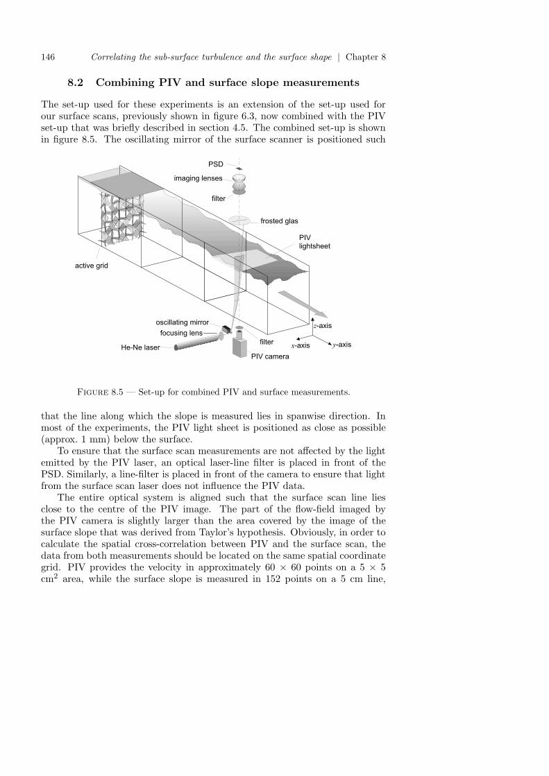
146 Correlating the sub-surface turbulence and the surface shape | Chapter 8
8.2 Combining PIV and surface slope measurements
The set-up used for these experiments is an extension of the set-up used forour surface scans, previously shown in figure 6.3, now combined with the PIVset-up that was briefly described in section 4.5. The combined set-up is shownin figure 8.5. The oscillating mirror of the surface scanner is positioned such
P S Di m a g i n g l e n s e s
f r o s t e d g l a s
a c t i v e g r i d
o s c i l l a t i n g m i r r o r
H e - N e l a s e rP I V c a m e r a
f i l t e r
P I Vl i g h t s h e e t
f i l t e r x - a x i sz - a x i s
y - a x i sf o c u s i n g l e n s
Figure 8.5 — Set-up for combined PIV and surface measurements.
that the line along which the slope is measured lies in spanwise direction. Inmost of the experiments, the PIV light sheet is positioned as close as possible(approx. 1 mm) below the surface.
To ensure that the surface scan measurements are not affected by the lightemitted by the PIV laser, an optical laser-line filter is placed in front of thePSD. Similarly, a line-filter is placed in front of the camera to ensure that lightfrom the surface scan laser does not influence the PIV data.
The entire optical system is aligned such that the surface scan line liesclose to the centre of the PIV image. The part of the flow-field imaged bythe PIV camera is slightly larger than the area covered by the image of thesurface slope that was derived from Taylor’s hypothesis. Obviously, in order tocalculate the spatial cross-correlation between PIV and the surface scan, thedata from both measurements should be located on the same spatial coordinategrid. PIV provides the velocity in approximately 60 × 60 points on a 5 × 5cm2 area, while the surface slope is measured in 152 points on a 5 cm line,

8.2 | Combining PIV and surface slope measurements 147
albeit non-equidistantly due to the harmonic nature of the scan. The grid onwhich the PIV data is located is coarser than that of the surface data and,consequently, it forms the basis for a new joint grid for both measurements. Inorder to calculate the desired cross-correlation functions, the surface slope datais interpolated onto this new grid by means of bi-linear interpolation. The joint
d o t s f o r c o o r d i n a t e d e f i n i t i o n
r e g i o n c o v e r e d b y c o r r e l a t i o n f u n c t i o n
Figure 8.6 — In order to perform the position calibration for PIVa plate with a dotted pattern is imaged with the PIV camera. Toenable the PIV camera to also see the 5 cm long surface-scan linethe line-filter in front of the camera has been removed. The length ofthe scanning line determines the extent of the region where the cross-correlation function can be calculated. The dots that lie outside ofthis line are very faint in the images. This is the result of the cameradiaphragm being set to its smallest setting, which was done to protectthe camera from the scanning laser. For the actual PIV calibration,the scanning laser was shut down, and the diaphragm was opened.
grid is defined by means of a picture taken with the PIV camera without itsline-filter, such as the picture shown in figure 8.6. In order to take this picture,a plate with a pattern of white dots against a black background is placed in thewater channel at the height of the PIV light sheet. Since the actual distancebetween the dots on the calibration plate is known, the corresponding distancein the image provides the calibration factor needed to convert pixels in the PIVimages to meters in the actual flow. This same calibration technique was usedin the PIV experiments described in chapter 4.
In order to match the spatial coordinates of the surface scan to those of thenew grid, it is vitally important to define the location of the origin and to alignthe orientation of the coordinate axes. The orientation of the axes in the PIVdata is defined by an L-shaped pattern of three larger dots on the calibrationplate. As was explained in section 6.3, the orientation of the coordinate systemin the surface scan data is dependent on the orientation of the axes of the

148 Correlating the sub-surface turbulence and the surface shape | Chapter 8
PSD. In practice, matching both to our coordinate systems involves rotatingand mirroring the axes. One of the three larger dots on the calibration plate,indicated in figure 8.6, is used as the origin for the new grid. The plate with thepattern is placed in the water-channel such that this particular dot lies on thechannel centre-line and at 2 m from the grid. The PIV camera is aligned suchthat this dot lies close to the centre of the camera image. After this, the surfacescanning set-up is aligned such that, with the oscillating mirror stationary inits centre position, the scanning beam is also aimed at this dot. This ensuresthat the position of the centre of the scan line corresponds to the origin inthe joint grid. Figure 8.6 was taken with the oscillating mirror switched on.The projection of the scan line on the calibration plate is clearly visible in theimage. Finally, its length defines the size of the square region in the PIV datathat corresponds to the surface scan.
r e f e r e n c e s i g n a l
f m i r r o r = 1 . 9 6 k H z
f s a m p l e = 3 0 0 k H z
s u r f a c e t r i g g e r s i g n a l
f p i v = 1 . 9 6 / 1 3 1 = 1 4 . 9 H z
t i m i n g u n i t
m i r r o r
P I V c a m e r a+ l a s e r A D C
P I V t r i g g e r s i g n a l
L E D t = 0
Figure 8.7 — Synchronising the surface scan and PIV measurements.

8.3 | A test case: vortex shedding 149
Not only should the data be located on the same spatial coordinates, butit should also be obtained at the same time. A given PIV snapshot needs to bematched to the correct part of the surface scan data and viceversa. Synchroni-sation is achieved by means of a purpose-built electronic timing unit, alreadybriefly mentioned before in section 6.3 as part of the surface scanning set-up.Now, in addition to providing trigger pulses at 300 kHz for the ADC used forthe surface slope scanner, once per 131 scan lines this timing unit triggers thePIV system. With approximately 2000 scan lines per second this means thatthe PIV system is triggered at close to its optimum frequency of 15 frame pairsper second. When the sampling of the surface scan data is started, a green LightEmitting Diode (LED)‡ located within the field of view of the PIV camera isbriefly illuminated, thereby setting time t = 0 for both measurements.
The cross-correlation between both measurements will show whether all ofthis is done correctly, since its maximum or minimum, depending on whetherwe are looking at the correlation Cs (between the slopes and the Euler terms)or Ce (between |ωz| and h), respectively, should lie in the origin.
8.3 A test case: vortex shedding
Because of the complicated timing and the difficulties in aligning both measure-ments, we have taken a look at a situation for which we know that sub-surfacevortices are closely linked to surface deformations, namely vortex shedding inthe wake of a surface-piercing vertical cylinder, as shown in the cartoon infigure 8.8. In chapter 2 we explained that a clear correlation between the sur-
Figure 8.8 — Cartoon of vortices being shed in the wake of a surface-piercing vertical cylinder.
face elevation and the vertical component of vorticity can be only expected ifthe vertical vorticity distributions in the sub-surface structures are cylindrical.In addition, the two-dimensional relation between the surface slopes and theEuler-terms of the sub-surface velocity field, equation (2.32), that is at the basisof Cs is only appropriate for quasi-stationary and columnar vortices.
The wake behind a cylinder has been investigated for more than a cen-tury. In a wide range of Reynolds numbers the wake is characterised by a
‡The diode is green in order for it to be visible to the PIV camera through its greenline-filter.

150 Correlating the sub-surface turbulence and the surface shape | Chapter 8
periodic shedding of columnar vortices, with their axes aligned with the cylin-der axis, and alternating positive and negative vorticity. For this type of flow,the Reynolds number is usually defined in terms of the cylinder diameter D andthe mean-stream velocity v0, so ReD = v0D/ν. The frequency f at which thevortices are shed is often non-dimensionalised in terms of the Strouhal number:St = fD/v0. The shedding frequency and, consequently, the Strouhal numberchange as the Reynolds number of the flow changes. An early detailed study ofthe effect of the Reynolds number on the wake and the Strouhal number, for alarge range of Reynolds numbers, was done by Roshko (1952), by means of ex-periments with hot-wire anemometry in a wind tunnel. For 40 < ReD < 150 theshed vortices form a stable so-called Von Karman vortex-street. In this rangeof Reynolds numbers the Strouhal number increases rapidly with increasingReynolds numbers. For 150 < ReD < 300 a number of different instabilitiescan occur in the wake, leading to the wake becoming more three-dimensionaland leading to large fluctuations in the Strouhal number. In Roshko’s experi-ments for ReD up to 104 periodic coherent vortices are still clearly visible in thewake, but beyond a distance of approximately 50 times the cylinder diameterthe wake becomes fully three-dimensional. In this range of Reynolds numbers,the Strouhal number is 0.21, practically independent of the Reynolds number.
For our experiments on vortex shedding the grid was removed from thewater channel and a cylinder with a diameter of 1.2 cm was placed in themeasurement section of channel instead. Measurements were done with fourdifferent mean stream velocities, corresponding to ReD = 225, 446, 902, and1860. The distance between our measurement location and the cylinder was40 cm, which is 33 times the cylinder diameter, and thus periodic vortices areclearly visible. Figure 8.9 shows four coinciding images of different propertiesof the flow, measured in the wake, for ReD = 1860. The surface slope field infigure 8.9 (a), derived from the surface scan by means of Taylor’s hypothesis,shows the presence of a circular area of low slope surrounded by a ring ofhigh slope: a depression in the surface. The corresponding surface slope fieldderived from PIV by means of the Euler equations, equation (8.2), in (b) showsa similar structure and the vorticity distribution shown in (d) has a clear peakat the same location. The integrated surface slope field in (c) shows that themaximum depth of the surface depression is only a few tenths of a millimeter.Evidently, the structure in question is a vortex, with an associated depressionin the surface above it. For this structure, the surface slope field derived fromthe sub-surface velocity field with equation (8.2), is very similar to the actuallymeasured surface slope field, both qualitatively and quantitatively. This canbe seen in more detail in figures 8.10 (a) through (d), which show a numberof cross-sections through the vortex core, for the vortex shown in figure 8.9.For these figures, the centre of the core has been defined as the point wherethe surface elevation has its minimum. The velocity profiles in spanwise andstreamwise direction, in figure (a), show that the location where the angular

8.3 | A test case: vortex shedding 151
-0.01
0
0.01
0.02
0.03
-0.02
-0.01
0
0.01
0.02
-0.02 -0.01 0 0.01 0.02
y (m
)
x (m)
(a)
-0.01
0
0.01
0.02
0.03
-0.02
-0.01
0
0.01
0.02
-0.02 -0.01 0 0.01 0.02
y (m
)
x (m)
(b)
0
5
10
15
20
x (m)
y (m
)
-0.02 -0.01 0 0.01 0.02
-0.02
-0.01
0
0.01
0.02
(c)
-1.5⋅10-4
-1.0⋅10-4
-5.0⋅10-5
0.0⋅100
5.0⋅10-5
x (m)
y (m
)
-0.02 -0.01 0 0.01 0.02
-0.02
-0.01
0
0.01
0.02
(d)
Figure 8.9 — Images of a vortex in the cylinder wake. (a) Sur-face slope field obtained from a measured PIV velocity field throughthe Euler equations, equation (8.2), with only one in four measuredvectors shown. The grey value represents the slope magnitude. (b)Corresponding image of the surface slope field obtained from a surfacescan, extended in streamwise direction by means of Taylor’s hypoth-esis and interpolated on the grid formed by the PIV data. (c) Theabsolute value of the vertical component of vorticity, obtained fromPIV. (d) The surface elevation (in meters) obtained from a surfacescan.

152 Correlating the sub-surface turbulence and the surface shape | Chapter 8
-0.04
-0.02
0
0.02
0.04
-1.5 -1 -0.5 0 0.5 1 1.5
u, v
(cm
/s)
x, y (cm)
-v(x)u(y)
(a)
-5
0
5
10
15
20
25
-1.5 -1 -0.5 0 0.5 1 1.5
|ωz|
(s-1
)
x, y (cm)
spanwisestreamwise
(b)
-0.04
-0.02
0
0.02
0.04
0.06
-1.5 -1 -0.5 0 0.5 1 1.5
h y
x (cm)
PIVscan
(c)
-0.15
-0.1
-0.05
0
0.05
-1.5 -1 -0.5 0 0.5 1 1.5
h (m
m)
x, y (cm)
spanwisestreamwise
(d)
Figure 8.10 — Cross-sections through the snapshots of the vortexshown in figure 8.9. The point (x, y) = (0, 0) is the point where thesurface elevation has its minimum. (a): Velocity profiles through thecore of the vortex. (b): Profiles of the vorticity. (c): The slope hy(x)as derived from PIV by means of the Euler equations, equation (8.2),and as actually measured. (d): Profiles of the elevation through thecore of the vortex
velocity equals zero coincides with the point of lowest elevation, but that thevortex is slightly asymmetric. Profiles of the vorticity in (b) show that thevorticity distribution in the vortex is not completely cylindrically symmetric,and that, consequently, the point of maximum vorticity does not coincide withthe minimum in elevation, as predicted by Zhang et al. (1999). Figure (c) showsprofiles (in spanwise direction) of the slope hy = ∂h/∂y derived from PIV bymeans of the Euler equations, equation (2.32), as well as the directly measuredslope, showing that both are broadly the same. Finally, figure (d) shows thatthe profiles of the surface elevation in the spanwise and the streamwise directionare practically identical. Not surprisingly, the vortex is roughly of the same sizeas the cylinder.

8.3 | A test case: vortex shedding 153
-0.2 0 0.2 0.4 0.6
-0.02-0.01
0 0.01
0.02 -0.02-0.01
0 0.01
0.02
-0.2 0
0.2 0.4 0.6
Cs
x (m) y (m)
Cs
(a)
-0.2 0 0.2 0.4 0.6
x (m)
y (m
)
-0.02-0.01 0 0.01 0.02
-0.02
-0.01
0
0.01
0.02
(b)
-0.4-0.2 0 0.2 0.4 0.6
-0.02-0.01
0 0.01
0.02 -0.02-0.01
0 0.01
0.02
-0.4-0.2
0 0.2 0.4 0.6
-Ce
x (m) y (m)
-Ce
(c)
-0.6-0.4-0.2 0 0.2 0.4
x (m)
y (m
)
-0.02-0.01 0 0.01 0.02
-0.02
-0.01
0
0.01
0.02
(d)
Figure 8.11 — Cross-correlation functions in the cylinder wake forReD = 1860. (a) and (b): Cross-correlation Cs between the measuredslopes and the slope field derived from simultaneous PIV measure-ments of the sub-surface velocity field by means of the Euler equa-tions, equation (8.2). (c) and (d): Cross-correlation Ce between thesurface elevation and |ωz|. Note that in (c) the vertical scale has beeninverted in order to better show the minimum.
The cross-correlations Cs and Ce, averaged over 800 subsequent frames, forthis same experiment are shown in figure 8.11. The correlation Cs between theslopes and the Euler terms, shown in figure 8.11 (a), has a distinctive peak witha height of close to 0.5, at (x, y) = (0, 0). This can also clearly be seen in thecorresponding contour plot in figure (b). Similarly, the correlation between theelevation and vorticity, correlation function Ce in figure (c) has a distinctivenegative peak with a depth of close to 0.5, with the corresponding contourimage shown in (d). That the peaks are located around (0, 0) demonstratesthat alignment of the grids of both measurements was successful and that thesynchronisation works as well. Let us emphasise that the correlations involvetwo-dimensional surfaces that were constructed from line measurements. In

154 Correlating the sub-surface turbulence and the surface shape | Chapter 8
figure 8.11 the correlation peaks have a circular cross-section only if we choosethe convection velocity needed for this construction equal to the mean flowvelocity.
The size of both peaks clearly suggests a fairly strong correlation betweenthe measured properties. However, the peak value also depends on the pa-rameters used for PIV. In chapter 4 we have seen that velocity gradients andvorticity that can be derived from PIV measurements depend on the PIV in-terrogation window size, the density of the grid, and the radius of optionalGaussian filtering.
Briefly, the effect of both the finite size of the interrogation window andthe extent of the Gaussian velocity filter is a spatial filtering of the velocityfield. Decreasing the size of the interrogation windows increases the spatialresolution. Decreasing the size also leads to an increase in the percentage ofbad vectors, and in practice this determines the minimum window size. In ourexperiments, as well as those in chapter 4, we use interrogation windows of32×32 pixels, which corresponds to an area of 2×2 mm2 in the actual flow, andwe use 50 % overlap between neighbouring windows. With these settings, wefound that the number of spurious vectors still lies below 1%. A final parameterthat can be chosen is the radius of the Gaussian filter, as defined in equation(4.41). It is clear that the cross-correlations we are concerned with here are alsobe influenced by the filtering. We expect that if the correlation between thevelocity field and the surface were to be perfect, the actually measured correla-tion would increase with increasing spatial filter size, would reach a maximum,and would then start to decrease again, as the filter size becomes larger thanthe size of the vortices. Figure 8.12 shows how the peak values Cs(0, 0) andCe(0, 0) of the cross-correlation functions, depend on the chosen value of σfor the Gaussian weighted averaging, for two different Reynolds numbers. For
0.1
0.2
0.3
0.4
0.5
0.6
0.7
0 0.005 0.01 0.015
Cs(
0,0)
σ (m)
ReD = 1860ReD = 902
(a)
-0.6
-0.5
-0.4
-0.3
-0.2
-0.1
0
0 0.005 0.01 0.015
Ce(
0,0)
σ (m)
ReD = 1860ReD = 902
(b)
Figure 8.12 — Peak value of the cross-correlation functions for theslopes (Cs) and the elevation (Ce) as a function of the radius of theGaussian filter used to filter the PIV results.

8.4 | Grid-generated turbulence 155
both Reynolds numbers, Cs(0, 0) has its maximum value for σ=7 mm, whichis close to the radius of the cylinder. Hence, the results shown in figure (8.11)have been obtained from Gaussian averaging the velocity field with σ=7 mm.Table 8.1 lists the peak values found for σ=7mm for three highest Reynoldsnumbers in our experiments. The table shows that, as the Reynolds numberincreases, the correlation we measure becomes stronger. For the fourth andlowest Reynold number in our experiments, ReD = 225, the correlation func-tions no longer showed any clear peaks, primarily as a result of noise. Thesurface deformations in that case are too small to still be picked up in outrsurface scan. Clearly, despite the difficulties in quantitatively interpreting the
Table 8.1 — Peak values of Cs and Ce as a function of the Reynoldsnumber for vortex shedding. The values of ReD follow from the mean-stream velocity measured in the experiment by means of PIV.
ReD Cs(0, 0) Ce(0, 0)
446 0.14 -9.3·10−2
902 0.24 -0.131860 0.54 -0.51
cross-correlation functions, as the Reynolds number increases and the vorticesin the wake become stronger, their surface signature becomes more and morevisible and the correlation between the surface shape and sub-surface velocityfield becomes stronger.
However, the most important conclusion that can be drawn from theseresults is that the difficult alignment of both measurement techniques as well asthe synchronisation is successful. We are capable of simultaneously measuringboth the surface shape and the sub-surface velocity field at the same location,and can calculate cross-correlations between properties of the surface and thesub-surface velocity field.
8.4 Grid-generated turbulence
Having seen that the synchronisation and alignment can be done successfully,we can now do similar experiments for grid-generated turbulence. In order tobe able to compare the turbulence results to those of the vortex-shedding, heretoo we chose σ=0.7mm.
Figure 8.13 shows measured cross-correlation functions Cs and Ce for activegrid-generated turbulence with a mean-stream velocity of 25.7 cm/s and pro-tocol (25opt). Even though the correlation functions are not as well-behaved

156 Correlating the sub-surface turbulence and the surface shape | Chapter 8
-0.04-0.02 0 0.02 0.04 0.06
-0.02-0.01
0 0.01
0.02 -0.02-0.01
0 0.01
0.02
-0.04-0.02
0 0.02 0.04 0.06
Cs
x (m) y (m)
Cs
(a)
-0.04-0.02 0 0.02 0.04 0.06
x (m)
y (m
)
-0.02-0.01 0 0.01 0.02
-0.02
-0.01
0
0.01
0.02
(b)
-0.04-0.02 0 0.02 0.04 0.06
-0.02-0.01
0 0.01
0.02 -0.02-0.01
0 0.01
0.02
-0.04-0.02
0 0.02 0.04 0.06
-Ce
x (m) y (m)
-Ce
(c)
-0.06-0.04-0.02 0 0.02 0.04
x (m)
y (m
)
-0.02-0.01 0 0.01 0.02
-0.02
-0.01
0
0.01
0.02
(d)
Figure 8.13 — Cross-correlation functions for active-grid-generatedturbulence with protocol (25opt). (a) and (b): Cross-correlation Cs
between the measured slopes and the slope field derived from simulta-neous PIV measurements of the sub-surface velocity field by means ofthe hydrostatic balance, equation (8.2). (c) and (d): Cross-correlationCe between the surface elevation and |ωz|. Note that in (c) the ver-tical scale has been inverted in order to better show the minimum.

8.4 | Grid-generated turbulence 157
0.01
0.02
0.03
0.04
0.05
0 0.005 0.01 0.015
Cs(
0,0)
σ (m)
activestatic
(a)
-0.04
-0.03
-0.02
-0.01
0
0 0.005 0.01 0.015
Ce(
0,0)
σ (m)
activestatic
(b)
Figure 8.14 — Peak value of the cross-correlations function, (a)Cs and (b) Ce, as a function of the width of the Gaussian filter.The active-grid-generated turbulence, with a mean-stream velocityof 0.257 m/s, was generated with protocol (25opt). The turbulencegenerated with the static grid had a mean-stream velocity of 0.174m/s.
as the corresponding correlation functions for vortex shedding, shown in figure8.11, especially towards the edges, they still show a clear peak at the origin.
In the previous section, we have seen that the peak-value of the cross-correlation function can be influenced by changing the value of σ in the Gaussianaveraging of the velocity field. Figure 8.14 shows the influence of σ on the peakvalues for active-grid-generated turbulence, as well as for turbulence generatedwith the static grid. Apart from the fact that the peak values are much smaller,the general trend is the same as that for vortex shedding shown in figure 8.12.
Figure 8.15 shows cross-correlation functions for active grid-generated tur-bulence with two lower mean stream velocities, and with accordingly modifiedforcing protocols. These correlation functions are broadly the same as thoseshown in figure 8.13, showing that, as the turbulence becomes weaker and,accordingly, the surface deformations become smaller peaks are still clearly vis-ible near the origin. As emphasised before, the use of reconstructed surfaces(through Taylor’s hypothesis) filters structures that move with the mean flowvelocity. From the rotation symmetry of our measured correlation peaks welearn that the measured correlations indeed gauge these structures. Surfacestructures which do not move with the mean flow, such as gravity-capillarywaves, would spoil this correlation.
The values found for the active grid, corresponding to the correlation func-tions shown in figures 8.13 and 8.15, as well as for static-grid-generated turbu-lence, are listed in table 8.2. Generally, with the exception of the static gridgenerated turbulence, similar to vortex shedding, an increase in mean-streamvelocity, and correspondingly an increase in the grid’s mesh Reynolds number

158 Correlating the sub-surface turbulence and the surface shape | Chapter 8
-0.04 0 0.04 0.08 0.12
x (m)
y (m
)
-0.02-0.01 0 0.01 0.02
-0.02
-0.01
0
0.01
0.02
(a)
-0.08-0.04 0 0.04 0.08 0.12
x (m)
y (m
)
-0.02-0.01 0 0.01 0.02
-0.02
-0.01
0
0.01
0.02
(b)
-0.04
0
0.04
0.08
x (m)
y (m
)
-0.02-0.01 0 0.01 0.02
-0.02
-0.01
0
0.01
0.02
(c)
-0.04
0
0.04
x (m)
y (m
)
-0.02-0.01 0 0.01 0.02
-0.02
-0.01
0
0.01
0.02
(d)
Figure 8.15 — Cross-correlation functions between the surface andthe sub-surface velocity field for active-grid-generated turbulence: (a)Cs and (b) Ce for a mean-stream velocity of 16.6 cm/s and forcingprotocol (15opt), (c) Cs and (d) Ce for a higher mean stream ve-locity of 22.1 cm/s and forcing protocol (20opt).

8.4 | Grid-generated turbulence 159
Table 8.2 — Peak values of Cs and Ce for different forcing condi-tions. The turbulence statistics for the active-grid generated turbu-lence, measured at 10 cm below the surface by means of LDV arelisted in table 3.2. The velocities listed here were measured by meansof PIV, just below the surface.
v0 (m/s) vrms (m/s) Cs(0, 0) Ce(0, 0)
static 0.174 5.4·10−3 3.0·10−2 -2.5·10−2
15opt 0.257 1.6·10−2 8.4·10−2 -4.3·10−2
20opt 0.212 1.4·10−2 6.0·10−2 -3.0·10−2
25opt 0.163 1.1·10−2 4.0·10−2 -1.6·10−2
leads to a decreasingly strong link between the surface shape and the sub-surfacevelocity field. The peak values are much smaller than the corresponding valuesfor vortex-shedding, listed in table 8.1.
It is likely that only structures up to a certain depth below the surfaceinfluence the surface shape. In order to study this in more detail, a series ofexperiments was done, in which the distance between the light sheet and thesurface was increased from its minimum value of approximately 1 mm up tomore than 2 cm. The peak values of the cross-correlation functions Cs andCe, evaluated with similar PIV settings, are shown in figures 8.16 (a) and (b),respectively. The figure shows that the peak value Cs(0, 0) of the correlationbetween the Euler terms and the surface slopes steadily decreases for increasing
0
0.02
0.04
0.06
0.08
0.1
0 2 4 6 8 10 12 14 16 18 20
Cs(
0,0)
-z (mm)
(a)
-0.06
-0.04
-0.02
0
0 2 4 6 8 10 12 14 16 18 20
Ce(
0,0)
-z (mm)
(b)
Figure 8.16 — Peak value of the cross-correlation functions Cs
(slopes) and Ce (elevation), for active grid-generated turbulence withprotocol (25opt), as a function of the depth below the surface.

160 Correlating the sub-surface turbulence and the surface shape | Chapter 8
depth. Although the statistical fluctuations of Ce(0, 0) are large, the overalltrend in figure 8.16 (b) is similar. The correlation between the elevation and thevertical component of vorticity also decreases for increasing depth. For depthsbelow 19 mm, the cross-correlation functions no longer show a clear maximumor minimum. This indicates that the depth of the layer in the turbulenceresponsible for deforming the surface, at least for turbulence generated withthis protocol, is approximately 2 cm. In chapter 3 we have measured velocityprofiles as a function of depth by means of Laser-Doppler-Velocimetry at thesame location. These profiles show that within a layer with a depth of a fewcm below the surface, the horizontal velocity fluctuations increase, whereasthe vertical fluctuations decrease. This is most notable in figure 3.13, whichshows that in a layer with a depth of 2 cm the ratio of vrms over wrms, i.e.of the horizontal fluctuation velocity over the vertical fluctuation velocity isdramatically increased. This is in agreement with the presence of a source-layer,first suggested by Hunt and Graham Hunt & Graham (1978) and discussedbefore in chapter 2. Apparently, that part of the surface deformation that isdirectly associated with the sub-surface turbulence, is primarily connected tolarge, pancake-like structures present within this source layer.
8.5 Conclusions
We have combined our existing surface scanning method with PIV, in order tomeasure the spatial correlation between the surface shape and the sub-surfacevelocity field. The main difficulties in combining these techniques lie in makingsure that the data in both measurement techniques is located on the same gridand is measured simultaneously. A further difficulty in our measurements iscaused by the fact that the surface scanning technique only provides the slopealong a line. In order to cross-correlate the surface slope measurements withthe two-dimensional images of the velocity field, measured with PIV, the lineshave been extended to two-dimensional images by means of Taylor’s frozenturbulence hypothesis.
We have tested our procedures in a vortex-shedding experiment and ob-tained a fairly strong correlation (C ≈ 0.5) between surface elevation and theabsolute value of the vorticity. For similar vortices in a vertical shear layer,Dabiri & Gharib (2001) and Dabiri (2003) measured a cross-correlation co-efficient between the vertical component of vorticity, which in their case wasprimarily negative, and the surface elevation of ≈ 0.8. For the Reynolds num-bers we considered in our cylinder wake experiments, the wake is turbulent, butstill shows clear periodic shedding of large vortices. As can be expected fromcolumnar vortices, we find a clear correlation between the surface slope and theEuler terms of the sub-surface velocity field. The cross-correlation coefficientsfound from this comparison are similar to those between vorticity and the ele-vation. Directly comparing our results to those of Dabiri et al. is complicated,

8.5 | Conclusions 161
since, unlike Dabiri et al., we did not use any conditions for the minimum mag-nitude of the vorticity or the elevation. We have also seen that the numericalvalue of the cross-correlation coefficient is influenced by the spatial filtering inPIV, which is not reported by Dabiri et al..
Similar measurements have been performed on grid-generated-turbulence.The only quantitative information on the cross-correlation coefficients for fullydeveloped three-dimensional turbulence were found by Tsai (1998), who sim-ulated turbulence generated by a horizontal shear layer. He found a cross-correlation coefficient between the magnitude of the vertical vorticity and thesurface elevation ≈ 0.5. The maximum value we found for grid-generated-turbulence was ≈ 0.04. The cross-correlation coefficient based on the hydro-static balance was higher, ≈ 0.08.
There is a clear discrepancy between Tsai’s correlation coefficients and themeasured values. Obviously, something is missing in the simulation, and weconclude that the surface shape is more than a reflection of some property ofthe velocity field beneath it. In chapter 7 we have shown that the surfaceis wrinkled by gravity-capillary waves that may originate from structures inthe sub-surface velocity field, but that travel with a relatively large velocityover the surface. These waves would spoil the correlations, and they may beabsent in Tsai’s numerical simulations. A subtle issue in our experimental pro-cedure is the invocation of Taylor’s frozen turbulence hypothesis to reconstructa two-dimensional image from line scans. This procedure favours structuresthat travel with the mean flow velocity. However, we believe that our mea-sured correlations are not affected strongly by this procedure. This was learnedfrom correlating individual line scans of the surface with lines in the mea-sured two-dimensional velocity field. Although the statistical fluctuations inthe measured correlations are larger, the maximum correlation coefficient didnot change much.
Tsai (1998) measured an even higher cross-correlation between surface-parallel vorticity (below the surface) and the surface elevation. He associatedthis with up-wellings and downdraughts. Sadly, with our current set-up, we can-not identify these structures, since we do not have access to the vertical compo-nent of the velocity, nor the surface parallel components of the vorticity. Thesecould in principle be accessed by placing the laser sheet vertically in the channel,instead of parallel to the surface. Such experiments are highly recommended ifthis subject is to be further investigated. Another more complicated option issimultaneously measuring all three components of the velocity in a plane. Thisis possible by means of stereoscopic PIV, with a practically unchanged exper-imental set-up. Measuring all components of the vorticity requires even morecomplicated measurements, for instance with simultaneous PIV measurementsin two closely-spaced parallel light-sheets, or with holographic PIV.
Finally, by changing the distance between the surface and the plane in whichwe measure the velocity field, we have seen that the correlation disappears below

162 Correlating the sub-surface turbulence and the surface shape | Chapter 8
a certain depth. This depth corresponds to that of the source-layer, a layer inwhich kinetic energy is redistributed from vertical velocity fluctuations intohorizontal fluctuations. The space-time spectra of the surface slope in chapter7 showed that part of the surface moved with the mean-stream velocity. Thepresence of peaks in the cross-correlations clearly shows that these deformationsindeed are directly connected to structures in the turbulence below the freesurface, specifically in the source layer.

9
General conclusions
The main goal of this thesis was to find out what the shape of the free surfaceabove turbulence reveals about the properties of the sub-surface turbulence.This was studied by means of detailed experiments in a water channel in whichwe measured properties of both the surface shape and the sub-surface turbu-lence.
In most of the experiments the turbulence was generated by means of anactive grid. Far below the surface and depending on the forcing protocol used tocontrol the grid, the generated turbulence was a reasonably close approximationof homogeneous and isotropic turbulence. Straightforward point measurementsof the surface offer insufficient information to understand the nature of thesurface, since due to the Doppler-effect it is impossible to untangle spatial andtemporal information. Hence, we have developed a novel technique to measurethe surface slope with a high resolution in space and time along a line onthe surface. These space-time measurements of the surface shape show thepresence of gravity-capillary waves above the turbulence, that can be identifiedthrough their dispersion relation. Spatial measurements of the surface haveallowed us to measure the isotropy of the surface. While isotropic turbulence israre in nature, the choice for isotropic turbulence in our experiments providescrucial information. We have seen that for turbulence that is isotropic far belowthe surface, the surface shape is isotropic as well. Furthermore, if we changethe forcing protocol such that the turbulence becomes anisotropic, the surfaceshape becomes anisotropic as well. This shows conclusively that the waves onthe surface are generated not directly by the grid, but locally by the turbulence,instead.
In previous studies on sub-surface turbulence, other researchers have shownthat deformations of the surface are coupled to low pressure in the cores ofsub-surface vortices, and in experiments on a vertical shear layer (Dabiri &Gharib, 2001; Dabiri, 2003) as well as in numerical simulations of turbulencegenerated by a horizontal shear (Tsai, 1998) have found correlation coefficients

164 General conclusions | Chapter 9
between the vertical component of vorticity and the elevation of ≈ 0.8 and≈ 0.5, respectively. In similar experiments, in which we combined our surfacescanning technique with Particle Image Velocimetry, we also find a correlationcoefficient of ≈ 0.5 for the turbulent wake behind a surface-piercing cylinder.However, although for our grid-generated turbulence a distinct correlation peakstill is visible, the correlation coefficient in that case is significantly smaller:< 0.1. The most obvious explanation for this discrepancy is the presence ofgravity-capillary waves.
That the turbulence excites waves is somewhat unexpected. Existing theoryon the generation of surface waves by turbulence predicts that they can onlybe generated if the fluctuation velocities in the turbulence exceed the minimumphase-velocity for gravity-capillary waves. In our experiments the fluctuationvelocities are an order of magnitude smaller. The mechanism for the generationof these waves remains unknown. However, our measurements do show that themajority of the waves on the surface have wavelengths that are approximatelythe same as the integral scale of the sub-surface turbulence and out of the widerange of scales present in the turbulence, only the largest scales are visible inthe surface shape.

Bibliography
Aarts, D.G.A.L., Schmidt, M. & Lekkerkerker, H.N.W. 2004 Directvisual observation of thermal capillary waves. Science 304, 847–850.
Adrian, R.J. 1996 Analysis of a laser doppler anemometer. In Fluid Mechanics
Measurements, 2nd edition (ed. R. J. Goldstein), pp. 175–299. Washington:Taylor & Francis.
Adrian, R.J. & Goldstein, R.J. 1971 Analysis of a laser doppler anemome-ter. J. Phys. E: Sci. Instr. 4, 505–511.
Andersen, A. 2003 Vortex flows with a free surface and random matrix theoryand acoustic resonances. PhD thesis, The Technical University of Denmark.
Batchelor, G.K. 1951 Pressure fluctuations in isotropic turbulence. Proc.
Cambridge Philos. Soc. 47, 359–374.
Bernal, L.P. & Kwon, J.T. 1989 Vortex ring dynamics at a free surface.Phys. Fluids A. 1, 449–451.
Bock, E.J. & Hara, T. 1995 Optical measurements of capillary gravity wavesusing a scanning laser slope gauge. J. Atmos. Oceanic Technol. 12, 395–403.
Borue, V., Orszag, S.A. & Staroslesky, I. 1995 Interaction of surfacewaves with turbulence: direct numerical simulations of turbulent open chan-nel flow. J. Fluid Mech. 286, 1–23.
Brocchini, M. & Peregrine, D.H. 2001 The dynamics of strong turbulenceat free surfaces. part 1. description,. J. Fluid Mech. 449, 225–254.
Brumley, B.H. & Jirka, G.H. 1987 Near-surface turbulence in a grid-stirredtank. J. Fluid Mech. 183, 235–263.
Calmet, I. & Magnaudet, J. 2003 Statistical structure of high-reynolds-number turbulence close to the free surface of an open-channel flow. J. Fluid
Mech. 474, 355–378.
166 BIBLIOGRAPHY
Comte-Bellot, G. & Corrsin, S. 1966 The use of a contraction to improvethe isotropy of grid-generated turbulence. J. Fluid Mech. 25, 657–682.
Cox, C. & Munk, W. 1954 Statistics of the sea surface derived from sunglitter. J. Marine Res. 16, 199–225.
Dabiri, D. 2003 On the interaction of a vertical shear layer with a free surface.J. Fluid Mech. 480, 217–232.
Dabiri, D. & Gharib, M. 2001 Simultaneous free surface deformation andnear surface velocity measurements. Exp. in Fluids 30, 381–390.
Dalziel, S.B., Hughes, G.O. & Sutherland, B.R. 2000 Whole-field den-sity measurements by ‘synthetic schlieren’. Exp. in Fluids 28, 322–335.
Dugan, J.P. & Piotrowski, C.C. 2003 Surface current measurements usingairborne visible image time series. Remote Sens. Environ. 84, 309–319.
Durst, F., Melling, A. & Whitelaw, J.H. 1981 Principles and Practice
of Laser-Doppler Anemometry, 2nd. edition. Academic Press.
Durst, F. & Stevenson, W.H. 1979 Influence of gaussian beam propertieson laser doppler signals. Applied Optics 18, 516–524.
Elenbaas, T. 2006 Writing lines in turbulent air using air photolysis andrecombination tracking. PhD thesis, Eindhoven University of Technology.
Fernando, H.J.S. & Hunt, J.C.R. 1997 Turbulence, waves and mixing atshear-free density interface. part1. a theoretical model. J. Fluid Mech. 347,197–234.
Forbes, C., Leman, K., Olson, D. & Brown, O. 1993 Eddy and wavedynamics in the south atlantic as diagnosed from geosat altimeter data. J.
Geophys. Res. 12, 297–314.
Forliti, D.J., Strykowski, P.J. & Debatin, K. 2000 Bias and precisionerrors of digital particle image velocimetry. Exp. in Fluids 28, 436–447.
Foucaut, J.M., Carlier, C. & Stanislas, M. 2004 Piv optimization forthe study of turbulent flow using spectral analysis. Meas. Sci. Tech. 15,1046–1058.
Foucaut, J.M. & Stanislas, M. 2002 Some considerations on the accuracyand frequency response of some derivative filters applied to particle imagevelocimetry vector fields. Meas. Sci. Tech. 13, 1058–1071.

BIBLIOGRAPHY 167
Frisch, U. 1995 Turbulence, The Legacy of A.N. Kolmogorov . CambridgeUniv. Press.
Fung, J.C.H., Hunt, J.C.R., Malik, N.A. & Perkins, R.K. 1992 Kine-matic simulation of homogeneous turbulence by unstead random fouriermodes. J. Fluid Mech. 236, 281–318.
Gardner, F.M. 1979 Phaselock Techniques, 2nd. edition. Wiley Interscience.
George, W.K., Beuther, P.D. & Arndt, R.E.A. 1984 Pressure spectrain turbulent free shear flow. J. Fluid Mech. 148, 155–191.
Gharib, M. 1994 Some aspects of near surface vortices. Appl. Mech. Rev 47,S157–S162.
Gharib, M. & Weigand, A. 1996 Experimental studies of vortex disconnec-tion and surface connection at a free surface. J. Fluid Mech. 321, 59–86.
Gledzer, E. 1997 On the Taylor hypothesis corrections for measured energyspectra of turbulence. Physica D 104 (2), 163–183.
H. Huang, H., Dabiri, D. & Gharib, M. 1997 On errors of digital particleimage velocimetry. Meas. Sci. Tech 8, 1427–1440.
Handler, R.A., Swean, T.F., Leighton, R.I. & Swearingen, J.D. 1993Length scales and the energy balance for turbulence near a free surface. AIAA
Journal 31, 1998–2007.
Hara, T., Bock, E.J. & Donelan, M. 1997 Frequency-wavenumber spec-trum of wind-generated gravity-capillary waves. J. Geophys. Res. 102, 1061–1072.
Hodges, B.R. & Street, R.L 1999 On simulation of turbulent nonlinearfree-surface flows. J. Comput. Phys. 151, 425–457.
Holland, T.K. 2001 Application of the linear dispersion relation with respectto depth inversion and remotely sensed imagery. IEEE Trans. Geosci. Remote
Sensing 39, 2060–2072.
Hunt, J.C.R. 1984 Turbulence structure and turbulent diffusion near gas-liquid interfaces. In Gas Transfer at Water Surfaces (ed. W. Brutsaert &G.H. Jirka), pp. 67–82. Reidel.
Hunt, J.C.R. & Graham, J.M.R. 1978 Free-stream turbulence near planeboundaries. J. Fluid Mech. 84, 209–235.

168 BIBLIOGRAPHY
Hurst, D. & Vassilicos, J.C. 2004 Experiments in fractal-induced turbu-lence. In Advances in Turbulence X (ed. H.I. Andersson & P.-A. Krogstad),pp. 355–358. Barcelona: CIMNE.
Imaichi, K. & Ohmi, K. 1983 Numerical processing of flow-visualisation pic-tures - measurement of two-dimensional vortex flow. J. Fluid Mech. 129,283–311.
Jahne, B., Klinks, J. & Waas, S. 1994 Imaging of short ocean wind waves:a critical theoretical review. J. Opt. Soc. Am. A 11 (8), 2197–2209.
Keane, R.D. & Adrian, R.J. 1990 Optimization of particle image velocime-ters. part i: double pulsed systems. Meas. Sci. Tech. 1, 1202–1215.
Keane, R.D. & Adrian, R.J. 1991 Optimization of particle image velocime-ters. part ii: multiple pulsed systems. Meas. Sci. Tech. 2, 963–974.
Keane, R.D. & Adrian, R.J. 1992 Theory of cross-correlation analysis ofpiv images. Appl. Sci. Res. 49, 191–215.
Kraichnan, R.H. 1967 Inertial ranges in two-dimensional turbulence.Phys. Fluids 10, 1417–1423.
Kraichnan, R.H. 1970 Diffusion by a random velocity field. Phys. Fluids 13,22–31.
Kumar, S. & Banerjee, S. 1998 Development and application of a hierarchi-cal system for digital particle image velocimetry to free-surface turbulence.Phys. Fluids 10, 160–177.
Kumar, S., Gupta, R. & Banerjee, S. 1998 An experimental investigationof the characteristics of free-surface turbulence in channel flow. Phys. Fluids
10, 437–456.
Kundu, P.K. 1990 Fluid Mechanics. Academic Press.
Kurata, K.T., Grattan, K.T.V., Uchiyama, H. & TanakaT, T. 1990Water surface measurements in a shallow channel using the transmitted im-age of a grating. Rev. Sci. Instrum. 6, 736–739.
Lecordier, B., Demare, D., Vervisch, L.M.J., Reveillon, J. &Trinite, M. 2001 Estimation of the accuracy of piv treatments for tur-bulent flow studies by direct numerical simulation of multi-phase flow. Meas.
Sci. Tech. 12, 1382–1391.
Lighthill, J. 1978 Waves in Fluids. Cambridge Univ. Press.

BIBLIOGRAPHY 169
Loewen, S., Ahlborn, B. & Filuk, A.B. 1986 Statistics of surface flowstructures on decaying grid turbulence. Phys. Fluids 29, 2388–2397.
Lourenco, L. & Krothapalli, A. 2000 True resolution piv, a mesh freesecond order accurate algorithm. In Proc. 8th Int. Symp. Appl. Laser Tech.
Fluid Mech., p. 13.5. Lisbon, Portugal.
Luff, J.D., Drouillard, T., Rompage, A.M., Linne, M.A. & j.R.Hertzberg 1999 Experimental uncertainties associated with particle imagevelocimetry (piv) based vorticity algorithms. Exp. in Fluids 26, 36–54.
Maassen, S.R. 2000 Self-organization of confined two-dimensional flows. PhDthesis, Eindhoven University of Technology.
Magnaudet, J. 2003 High-reynolds-number turbulence in a shear-free bound-ary layer: Revisting the hunt-graham theory. J. Fluid Mech. 484, 167–196.
Makita, H. 1991 Realization of a large scale turbulence field in a small windtunnel. Fluid Dyn. Res. 8, 53–64.
van Manen, A.D. Schwarz 1992 Coherent structures over grooved surfaces.PhD thesis, Eindhoven University of Technology.
McWilliams, J.C. 1984 The emergence of isolated coherent vortices in tur-bulent flow. J. Fluid Mech. 146, 21–43.
Mohamed, S.M. & LaRue, J.C. 1990 The decay power law in grid-generatedturbulence. J. Fluid Mech. 291, 195–214.
Monin, A. & Yaglom, A.M. 1975 Statistical Fluid Mechanics VOL II . MITPress.
Mydlarski, L. & Warhaft, Z. 1990 On the onset of high-reynolds-numbergrid-generated wind tunnel turbulence. J. Fluid Mech. 320, 331–368.
Nagaosa, R. 1999 Direct numerical simulation of vortex structures and tur-bulent scalar transfer across a free surface in a fully developed turbulence.Phys. Fluids 11, 1581–1595.
Nagaosa, R. & Handler, R.A. 2003 Statistical analysis of coherent vorticesnear a free surface in a fully developed turbulence. Phys. Fluids 15, 375–394.
Pan, Y. & Banerjee, S. 1995 A numerical study of free-surface turbulencein channel flow. Phys. Fluids 7, 1288–1290.
Pearson, B.R., Krogstad, P.-A. & van de Water, W. 2002 Measure-ments of the turbulent energy dissipation rate. Phys. Fluids 14, 1288–1290.

170 BIBLIOGRAPHY
Perot, B. & Moin, P. 1995 Shear-free turbulent boundary layers. part 1.physical insights into near-wall turbulence. J. Fluid Mech. 295, 199–227.
Phillips, O.M. 1957 On the generation of waves by turbulent wind. J. Fluid
Mech. 4, 417–445.
Phillips, O. M. 1980 The Dynamics of the Upper Ocean, 2nd edition. Cam-bridge Univ. Press.
Poorte, R.E.G. 1998 On the motion of bubbles in active grid generated tur-bulent flows. PhD thesis, University Twente.
Poorte, R.E.G. & Biesheuvel, A. 2002 Experiments on the motion of gasbubbles in turbulence generated by an active grid. J. Fluid Mech. 461, 127–154.
Pope, S.B. 2000 Turbulent Flows. Cambridge Univ. Press.
Pulles, C.J.A. 1988 Drag reduction of turbulent boundary layers by meansof grooved surfaces. PhD thesis, Eindhoven University of Technology.
Raffel, M., Willert, C.E. & Kompenhans, J. 1998 Particle Image Ve-
locimetry, A Practical Guide. Springer-Verlag.
Rashidi, M. & Banerjee, S. 1988 Turbulence structure in open channelflows. Phys. Fluids 31, 2491–2503.
Rood, E.P. & Katz, J., ed. 1994 Free-Surface Turbulence, American Societyof Mechanical Engineers, Fluids Engineering Division. FED-Vol. 181.
Roshko, A. 1952 On the development of turbulent wakes from vortex sheets.PhD thesis, California Institute of Technology.
Sajjadi, S.G 2002 Vorticity generated by pure capillary waves. JFM 459,277–288.
Sarpkaya, T. 1996 Vorticity, free surface, and surfactants. Annu. Rev. Fluid.
Mech. pp. 83–128.
Sarpkaya, T. & Suthon, P. 1991 Interaction of a vortex couple with a freesurface. Exp. in Fluids 11, 205–217.
Scarano, F. & Riethmuller, M.L. 1999 Iterative multi-grid appraoch inpiv image processing with discrete window offset. Exp. in Fluids 26, 513–523.
Senet, C.M., Seemann, J. & Ziemer, J. 2001 The near-surface currentvelocity determined from images sequences of the sea surface. IEEE Trans.
Geosci. Remote Sensing 39, 492–505.

BIBLIOGRAPHY 171
Settles, G.S. 2001 Schlieren and Shadowgraph Techniques, Visualizing Phe-
nomena in Transparent Media. Springer-Verlag.
Shen, L., Zhang, X., Yue, D.K.P. & Triantafyllou, G.S. 1999 Thesurface layer for free-surface turbulent flows. J. Fluid Mech. 386, 167–212.
Song, M., Bernal, L.P. & Tryggvason, G. 1992 Head-on collision of alarge vortex ring with a free surface. Phys. Fluids A. 4, 1457–1466.
Stammer, D. 1997 Global characteristics of ocean variability from regionaltopex/poseidon altimeter measurements. J. Phys. Oceanogr. pp. 1743–1769.
Teixeira, M.A.C. 2000 Interaction of turbulence with a free surface. PhDthesis, University of Reading.
Teixeira, M.A.C. & Belcher, S.E. 2000 Dissipation of shear-free turbulencenear boundaries. J. Fluid Mech. 422, 167–191.
Titov, V., Rabinovich, B., Mofjeld, H.O., Thomson, R.E. &Gonzalez, F.I. 2005 The global reach of the 26 december sumatra tsunami.Science 309, 2045–2048.
Tsai, W.-T. 1998 A numerical study of the evolution and structure of a tur-bulent shear layer under a free surface. J. Fluid Mech. 354, 239–276.
Tsai, W.-T. & Yue, D.K.P. 1996 Computation of non-linear free-surfaceflows. Annu. Rev. Fluid Mech. 28, 249–278.
Walker, D.T., Chen, C.-Y. & Willmarth, W.W. 1995 Turbulent struc-ture in free-surface jet flows. J. Fluid Mech. 291, 223–261.
Walker, D.T., Leighton, R.I. & Garza-Rios, L.O. 1996 Shear-free tur-bulence near a flat free surface. J. Fluid Mech. 320, 19–51.
Wehousen, J.V. & Laitone, J.C. 1960 Surface waves. In Encyclopedia of
Physics, band IX (ed. S. Flugge & C. Truesdell), pp. 446–778. Springer Ver-lag.
Weigand, A. 1996 Simultaneous mapping of the velocity and deformation fieldat a free surface. Exp. in Fluids 20, 358–364.
Westerweel, J. 1993 Digital particle image velocimetry, theory and applica-tion. PhD thesis, Delft University of Technology.
Westerweel, J. 1994 Efficient detection of spurious vectors in particle imagevelocimetry data. Exp. in Fluids 16, 236–247.

172 BIBLIOGRAPHY
Westerweel, J., Dabiri, D. & Gharib, M. 1997 The effect of a discrete win-dow offset on the accuracy of cross-correlation analysis of digital piv record-ings. Exp. in Fluids 23, 20–28.
Westra, M.-T., Binks, D. J. & van de Water, W. 2003 Patterns ofFaraday waves. J. Fluid Mech. 496, 1–32.
Willert, C.E. & Gharib, M. 1991 Digital particle image velocimetry. Exp. in
Fluids 10, 181–193.
Willert, C.E. & Gharib, M. 1997 The interaction of spatially modulatedvortex pairs with free surfaces. J. Fluid Mech. 345, 227–250.
Zhang, C., Shen, L. & Yue, D.K.P 1999 The mechanism of vortex connec-tion at a free surface. J. Fluid Mech. 384, 207–241.
Zhang, X. 1995 Capillary-gravity and capillary waves generated in a windwave tank: observations and theories. J. Fluid Mech. 289, 51–82.
Zhang, X. & Cox, C.S. 1994 Measuring the two-dimensional structure of awavy water surface optically: A surface gradient detector. Exp. in Fluids 17,225–237.

Summary
Surprisingly little is known about the statistical nature of the shape of a freesurface above turbulence and about how this shape depends on the propertiesof the turbulence.The main focus of this thesis is on experiments in which the statistical prop-erties of both the surface and the turbulence are measured with a number ofdifferent techniques. The experiments are done in a free-surface water-channel,in which turbulence is generated with an active grid. This active grid consists ofan array of horizontal and vertical rods through the channel, with small wingsattached to them. The rods are individually driven by electric motors, accord-ing to a certain forcing protocol, thereby adding energy to the turbulence. Amajor advantage of an active grid is that, by changing this protocol, the prop-erties, such as the intensity and the isotropy, of the generated turbulence canbe changed. These properties were measured by means of Laser-Doppler Ve-locimetry. The turbulence behind the active grid is much more intense thanturbulence generated by a more common static grid. The maximum Taylor-based Reynolds number reached with the active grid (at 40 times the mesh sizebehind the grid) was Reλ = 256, compared to Reλ = 70 with a similarly dimen-sioned static grid. Consequently, the active-grid-generated turbulence showsclear Kolmogorov scaling behaviour over a relatively wide range of scales. Thestronger turbulence also leads to stronger surface deformations.In order to characterise the shape of the surface, it is essential to measurethe surface shape with a high resolution both in space and time. In order toachieve this, a novel technique has been developed, based on refraction of alaser beam that shines through the surface. The deflection of the beam dueto the local surface slope is measured by means of an optical position sensingdevice. The beam is swept along a line by means of a rapidly oscillating mirror(with a frequency of close to 2 kHz). This allows measurements of the surfaceslope at multiple points along the line as a function of time. This surfacescanning technique can be combined with Particle Image Velocimetry (PIV),which provides snapshots of the velocity field and the vertical component ofvorticity in horizontal planes just below the surface. This combination allows usto simultaneously measure the velocity field and the surface deformations aboveit. PIV is based on the cross-correlation of the intensity distributions in images
173

174 SUMMARY
of particles suspended in the flow, that are illuminated by a thin laser light sheet.When applying PIV to turbulence, it is important to realise that the velocityfield that can be obtained with PIV is a spatially averaged representation ofthe actual velocity field. The effect this averaging has on measured turbulenceproperties is investigated by means of kinematic simulations, in which realisticturbulent velocity fields, with a prescribed energy spectrum, are generated.Synthetic particle images derived from these fields are evaluated by means of aPIV algorithm and the velocity spectrum is calculated. Comparing this to theprescribed spectrum clearly shows the averaging, and allows us to predict itsinfluence on other measured turbulence properties.The turbulence generated by our grid is not strong enough to lead to verylarge deformations of the surface. The measured changes in elevation are lessthan 1 mm. In that case, somewhat naively, one would expect the surfacedeformations to be primarily associated with sub-surface vortices. In the coreof a vortex the magnitude of the vorticity is high, while the pressure is low.This low pressure causes a dimple in the surface above the vortex. This effectcan, for instance, be seen when stirring a cup of tea or in the wake behindbridge pillars in a river. Consequently, in simultaneous measurements of thesurface shape and the sub-surface velocity field one would expect to find arelatively large correlation between the vertical component of vorticity and thesurface elevation. Indeed, our measurements show that relatively strong vorticesin the turbulence do deform the surface. However, the measured correlationcoefficients are low (< 0.1). Spectra of the surface slope in space and timeshow that, instead of being connected directly to sub-surface structures, muchof the surface actually consists of gravity-capillary waves, i.e. regular surfacewaves. For surface waves, there is a clear relation between their wavelength andtheir frequency. This relation can be identified in our spectra. The presenceof these waves is somewhat surprising, since resonant wave growth can only beexpected to occur if the fluctuation velocities in the turbulence are larger thanthe minimum phase velocity of the waves (≈ 0.23 m/s), while the measuredfluctuation velocities in our turbulence are an order of magnitude smaller. Aremarkable feature of the waves above the turbulence is that they travel in alldirections across the surface. In fact, provided that the turbulence far below thesurface is isotropic, the surface shape itself is isotropic as well. In other words,statistically, the waves on the surface are the same in every direction. Wecan change this by changing the forcing protocol of the active grid such thatthe turbulence becomes anisotropic. In that case the surface shape becomesanisotropic as well. This is a clear indication that the surface waves are excitedlocally by the turbulence. We have found evidence to suggest that the waves areexcited by the largest structures in the turbulence. As a consequence of this,the surface shape does not reflect the wide range of scales in the sub-surfaceturbulence, but instead exhibits waves primarily with wavelenghts close to theintegral scale of the turbulence.

Samenvatting
Er is verbazingwekkend weinig bekend over hoe de statistische eigenschappenvan de vorm van een vrij oppervlak boven turbulentie afhangen van de turbu-lentie zelf. Het zwaartepunt van dit proefschrift ligt bij experimenten, waarinde eigenschappen van het oppervlak en van de turbulentie worden gemeten meteen aantal verschillende technieken. De experimenten zijn gedaan in een wa-terkanaal, waarin turbulentie wordt opgewekt met behulp van een actief rooster.Dit rooster bestaat uit horizontale en verticale assen die door het kanaal steken.Aan deze assen zijn vaantjes bevestigd. De individuele assen kunnen onafhanke-lijk van elkaar worden bewogen met behulp van electro-motoren die volgens eenbepaald forcerings-protocol worden aangestuurd. Door dit roeren wordt de tur-bulentie sterker en door het aanpassen van het protocol kunnen de eigenschap-pen van de turbulentie, zoals de intensiteit en isotropie, worden beınvloed. Deeigenschappen van de turbulentie zijn gemeten met behulp van Laser-Dopplersnelheidsmetingen. Dat de turbulentie achter het actieve rooster intenser isdan die achter een regulier statisch rooster blijkt onder andere uit het geme-ten Reynolds-getal gebaseerd op de Taylor lengte-schaal van de turbulentie. Demaximum waarde voor het actieve rooster (op 40 keer de maasgrootte achter hetrooster) is Reλ = 256, terwijl voor een statisch rooster van dezelfde afmetingenReλ = 70 werd gemeten. De sterkere turbulentie vertoont duidelijk schalings-gedrag over een relatief groot schaal-bereik en leidt tot sterkere vervormingenvan het oppervlak.Om te begrijpen wat er aan het oppervlak gebeurt is het belangrijk om de vormvan het oppervlak te meten, met een hoge resolutie in zowel de tijd als in deplaats. Hiervoor is een nieuwe techniek ontwikkeld. De lokale helling van hetoppervlak wordt bepaald aan de hand van de uitwijking van een laserbundel diewordt gebroken aan het oppervlak. De uitwijking wordt gemeten met behulpvan een zogenaamd optisch position sensing device (een plaats-gevoelige detec-tor). Een oscillerend spiegeltje laat de bundel snel heen-en-weer zwiepen (meteen frequentie van bijna 2 kHz), zodat de helling als functie van de tijd wordtgemeten in meerdere punten op een lijn. De oppervlakte metingen kunnen wor-den gecombineerd met Particle-Image Velocimetry (PIV). Met deze techniekkunnen moment-opnamen van het snelheidsveld onder het oppervlak wordengemaakt. Zo kunnen we gelijktijdig de snelheid en de vorm van het opper-

176 SAMENVATTING
vlak meten. PIV werkt aan de hand van het correleren van digitale foto’s vande deeltjes-verdeling in de stroming, waarbij de deeltjes worden verlicht meteen dun laser-lichtvlak. Wanneer PIV wordt toegepast op turbulentie is hetvan belang dat een met PIV gemeten snelheidsveld een ruimtelijk gemiddeldeweergave is van het echte snelheidsveld. Deze middelling heeft gevolgen voorde gemeten eigenschappen van de turbulentie. Dit is nader onderzocht aan dehand van kinematische simulaties. Hierin worden realistische snelheidsveldenmet een voorgeschreven energiespectrum berekend. Deze vormen de basis voorsynthetische afbeeldingen van de deeltjes-verdeling in de stroming. Deze kun-nen worden verwerkt met een PIV-algoritme en vervolgens kan het energiespectrum worden berekend. Een vergelijking hiervan met het oorspronkelijkespectrum laat de middelling duidelijk zien en maakt het mogelijk de invloedvan de middelling op andere eigenschappen van de turbulentie te voorspellen.De turbulentie in ons kanaal is niet sterk genoeg om het oppervlak sterk te ver-vormen. De gemeten variaties in de hoogte zijn minder dan 1 mm. Enigszinsnaıef valt in dat geval te verwachten dat vervormingen van het oppervlak vooralontstaan als gevolg van wervels onder het oppervlak. In een wervel is de vor-ticiteit groot en de druk laag. Die lage druk kan ervoor zorgen dat er in hetoppervlak boven een wervel een deukje ontstaat. Op grond hiervan verwachtje een vrij sterke correlatie tussen de verticale component van de vorticiteit ende hoogte van het oppervlak. Onze metingen laten inderdaad zien dat sterkewervels het oppervlak vervormen, maar de gemeten correlatie-coefficienten zijnklein (< 0.1). Er is dus meer aan de hand. Spectra van de helling van hetoppervlak in plaats en tijd laten zien dat de vorm van het oppervlak niet directgekoppeld is aan de turbulentie, maar voor een groot deel bestaat uit capillairezwaartekrachts-golven. Voor dit soort normale oppervlakte-golven is er eenduidelijk verband tussen de golflengte en de frequentie. Deze relatie is terugte zien in de gemeten spectra van het oppervlak. Dat er golven ontstaan isenigszins onverwacht. Een voorwaarde voor het resonant groeien van golven isdat de snelheidsfluctuaties in de turbulentie groter zijn dan de minimum fase-snelheid van de golven (≈ 0.23 m/s). De door ons gemeten fluctuaties zijnechter een orde van grootte kleiner. Heel bijzonder is dat de golven in allerichtingen over het oppervlak reizen. Sterker nog, wanneer de turbulentie veronder het oppervlak isotroop is, dan is het oppervlak zelf ook isotroop. Datwil zeggen, de statistische eigenschappen van de golven zijn in alle richtingenhetzelfde. Door het forcerings-protocol van het actieve rooster zodanig te veran-deren dat de turbulentie anisotroop wordt, wordt het oppervlak ook anisotroop.Dit toont aan dat de golven lokaal worden aangeslagen door de turbulentie. Wehebben aanwijzingen gevonden dat hierbij vooral de grotere structuren in destroming een rol spelen. In de vorm van het oppervlak is niets terug te zienvan de kleinere schalen in de turbulentie. De vorm wordt gedomineerd doorgolven met een golflengte die vergelijkbaar is met de integrale lengte-schaal vande stroming.

Dankwoord / Acknowledgements
Het hier beschreven werk had niet kunnen worden gedaan zonder de hulp vaneen groot aantal mensen. Hoewel mijn gezondheid me af en toe in de steek liet,lieten onderstaande mensen me niet zakken. In de eerste plaats wil ik Willemvan de Water bedanken. Zonder Willems drive, duwtjes in de rug, “hands-onapproach”, soms wilde maar meestal zinnige ideeen en natuurlijk zijn vermaarde“Fortran-programmes of everything” zou dit werk nooit gelukt zijn. Onze somsheftige discussies, met veel handgebaren, vage krijttekeningen op het bord envooral ook veel misverstanden waren toch vaak verhelderend en ik zal ze in detoekomst dan ook enorm missen. GertJan van Heijst wil ik vooral bedankenvoor het vertrouwen dat hij me gegeven heeft en voor de goede raad en hulpop die hij me gaf op de momenten dat ik zelf het vertrouwen dreigde kwijt teraken. Hoewel het door alle experimentele complicaties er niet van is gekomenom numerieke simulaties aan free-surface turbulence te doen en zijn rol in hetproject hierdoor kleiner is geworden dan hij zelf misschien gewild had, wil ikook Herman Clercx bedanken. Hij hield de vinger aan de pols en heeft, zekerin het begin van het project, menige hobbel weten glad te strijken.I owe many thanks to Carl Tipton for his friendship and the many lively dis-cussions that we had about cross-spectral densities, the peculiarities of DutchEnglish, (the) Dutch in general, and pretty much anything else one could pos-sibly think of. I also want to thank Anders Andersen for his valuable ideas andinput in trying to find the models described in chapter 2. I enjoyed our worktogether.Een aantal studenten heeft een directe bijdrage geleverd aan het werk in ditproefschrift: Hubert van Luytelaar als afstudeerder en Koos Delescen, Gijs vander Heijden en Jochem Nietsch als stagairs. Ik hoop dat jullie iets van desamenwerking hebben opgestoken. Ik in ieder geval wel van jullie.Ik heb heel veel hulp gehad van onze onmisbare technici: Gerald Oerlemans voorhet actieve rooster, de bevestiging van de LDV opstelling en onderdelen voorPIV, Freek van Uittert, met name voor de aansturing van het actieve rooster,Ad Holten voor de dataverwerking voor LDV en zijn onmisbare hulp bij hetontwikkelen van de oppervlaktemeettechniek (file-headers!) en Gert van derPlas voor zijn ondersteuning met PIV, LDV en het hele FreeBSD computer-gebeuren. Hun bijdragen zijn niet zo beperkt of zo strikt gescheiden als het

178
voorgaande suggereert. Het hele team heeft me op allerlei manieren geholpen,niet alleen door aan te pakken, maar ook door met me mee te denken en (nietin de laatste plaats) door hun grote rol in de goede sfeer in de groep. In ditlicht bezien mogen ook Pim Sluyter, Jan Willems, Gerard Trines en HermanKoolmees niet ontbreken. Onze bezoekjes aan de Chinees op de Kruisstraatzal ik niet licht vergeten. Verder zijn veel technische klussen opgeknapt doorde Centrale Technische Dienst en door de werkplaats van N-laag, onder debezielende leiding van Marius Bogers.Zonder het secretariaat, afwisselend bezet door Anita, Brigitte en Marjan, zouik er regelmatig een zootje van hebben gemaakt. Administratie en geregelzijn niet mijn favoriete bezigheden, maar gelukkig kon ik op het secretariaatvertrouwen.Ik wil ook Ruben Trieling, Bernard Geurts, Rini van Dongen en Mico Hirschbergbedanken. Hoewel ze formeel niet bij mijn project betrokken waren, waren zein de praktijk maar al te bereid me van goede raad te voorzien. Voor goederaad in meer algemene zin kon ik ook altijd rekenen op Toon Wouters.Natuurlijk wil ik ook mijn mede-promovendi en veel van de studenten diedoor de jaren heen bij ons gewerkt hebben bedanken. Met sommigen heb iknatuurlijk meer contact gehad dan met anderen. De gezamelijke theepauze’s middags was vaak het gezelligste moment van de dag en de daarbij gevoerdegesprekken over “life, the universe, and everything” waren meestal komisch enzondermeer erg levendig. Na zo’n pauze kon ik er weer een aantal uurtjes te-genaan. Ik ga verder geen lange opsomming van namen geven, maar mijn tweekamergenoten mogen niet onvernoemd blijven: Robin Schoemakers en Laurensvan Bokhoven (met waarschijnlijk het netste bureau binnen de TU). We hebbenheel wat uurtjes samen doorgebracht en ook heel wat afgelachen.Tja, en waar zou ik zijn zonder mijn vriendenclub? Harm, Thijs, Maarten,Csaba, Karel en Doryan, Maikel en Fenna. Zij wisten iedere keer op donderdag-avond bij die andere Chinees op de Kruisstraat (King Hung) de zaken in hetjuiste perspectief (of toch net het verkeerde?) te plaatsen. Dat was onont-beerlijk voor mijn gezondheid, hoewel die er de ochtend erna soms ook onderte lijden had. Gon Bao Kai met Palm valt niet altijd even goed. Harm, ein-delijk heb ik een geschikte gelegenheid: “Rene, Edith, the bedknobs, they areblinking!” (het nep-accent moet je er zelf bij bedenken). Ik wil Ben bedanken,onder andere voor de onvergetelijke concerten van Peter Gabriel waar we samennaartoe geweest zijn. Daarnaast wil ik ook Antoin bedanken, al toen ik zevenjaar oud was mijn beste vriend.Tenslotte wil ik mijn ouders en mijn zus bedanken voor hun onvoorwaardelijkeliefde. Zonder hun steun zou dit proefschrift er niet zijn gekomen.

Curriculum Vitae
July 16, 1975Born in Kerkrade, The Netherlands
1987-1993St. Antonius Doctor College, Kerkrade (VWO)
1993-2000Student of Applied Physics, Eindhoven University of Technology.
• Traineeship in the group Equilibria and Transport in Plasmas,Diode Laser Absorption of Balmer-α in the Expanding Hydrogen
Plasma
• Masters thesis in the group Vortex Dynamics and Turbulence,The Free-Surface Evolution of Half Vortex Rings
2000-2006PhD Candidate in the group Vortex Dynamics and Turbulence, Depart-ment of Applied Physics, Eindhoven University of Technology,Experiments on Free-Surface Turbulence
May 2006Postdoctoral Research Fellow, School of Engineering Sciences, Universityof Southampton, UK
