1

Explaining White Polarization in the 2016 Vote for President: The Sobering Role of Racism and Sexism

Brian F. Schaffner

University of Massachusetts Amherst schaffne@polsci.umass.edu

Matthew MacWilliams

University of Massachusetts Amherst

Tatishe Nteta University of Massachusetts Amherst

\body

2

The 2016 presidential campaign featured candidates who both explicitly put issues of

race and gender at the forefront of the discourse. Notably, 2016 also witnessed the largest gap

between the presidential vote preferences of college- and non-college educated whites since

1980. While Trump enjoyed just a four-point margin over Clinton among whites with a college

degree (10 points smaller than Romney’s margin over Obama among that group in 2012), his

advantage among non-college educated whites was nearly 40 points. This gap between college-

and non-college educated whites was possibly the single most uniquely important divide

documented in 2016, and this point was succinctly made by the New York Times’ Nate Cohn

who declared, “Donald J. Trump won the presidency by riding an enormous wave of support

among white working-class voters.”

While many election post-mortems were quick to make note of the education gap among

whites in terms of presidential vote choice in 2016, explanations for the origins of this gap were

a subject of greater debate. Two prominent explanations have been offered. The first is that white

working class Americans have been left behind during the economic recovery that took place

during the Obama presidency. Trump’s populist economic message, focusing on protectionism

and other policies to help working people, resonated with this group (e.g. Tankersley 2016). A

second explanation is that Trump’s willingness to make explicitly racist and sexist appeals

during the campaign, coupled with the presence of an African American president and the first

major party female nominee, made racism and sexism a dividing line in the vote in this election

(e.g. Sides and Farrell 2016). This led less educated whites, who tend to exhibit higher levels of

sexism and racism, to support Trump, while more educated whites were more supportive of

Clinton (Schuman et al 1997; Glick et al. 2002).

3

In this paper, we use data from a national survey conducted during the final week of

October to adjudicate between these two popular explanations. Using unique measures of

attitudes on racism and sexism, coupled with a question designed to tap into dissatisfaction with

personal economic conditions, we are able to determine to what extent each of these explanations

helped to explain vote choices in 2016 and, ultimately, whether either of these explanations can

explain the education gap in vote choice among whites. We find that while economic

dissatisfaction was an important part of the story, racism and sexism were much more impactful

in predicting support for Trump among white voters and more specifically both sexism and

racism explain close to two-thirds of the educational gap among white voters in the 2016

presidential vote.

Explaining the Education Divide Among Whites

As noted above, there has been a wealth of media attention focused on the education gap

and class differences among whites in predicting presidential vote choice in 2016 (see Silver

2016; McGill 2016). However, less attention has been paid to the history of this divide in

American presidential politics. Figure 1 plots the Republican share of the two-party vote for

president among whites with and without a college degree in each presidential election since

1980. These data are from the national exit polls, as compiled by the New York Times.1 Note that

white voting behavior in presidential elections was rather similar from 1980 through 1996,

regardless of education. Indeed, in none of these elections was there more than a five percentage

point difference in how college and non-college educated whites voted. In 2000, a small but

notable gap did begin to emerge, with non-college whites providing more support for the

1Data accessed from https://www.nytimes.com/interactive/2016/11/08/us/politics/election-exit-polls.html. Site only includes exit polls conducted from 1980 – 2016.

4

Republican presidential nominee. This gap remained relatively small, ranging from 5 to 7 points

in the elections held from 2000 to 2012.

In 2016, however, the gap in vote preferences between college and non-college whites

widened considerably to 18 points, nearly three-times larger than it had been in any election

during the series. Importantly, this 18-point gap resulted from an apparent polarization among

whites; college-educated whites became more supportive of Clinton than they had been for

Obama in 2012, while whites without a college degree moved even more dramatically toward

Trump. In fact, Trump won over 70% of the two-party vote among whites without a college

degree, which easily exceeded the performance of any Republican going back to at least 1980.

His success with this group was particularly important in the three states that ultimately decided

the election – Wisconsin, Michigan, and Pennsylvania. According to exit polls, in those three

states, whites without a college degree made up between 40 and 47% of the electorate and in

each state they favored Trump by about 30-points over Clinton.

The emergence of the education gap in vote choice among whites after the turn of the

century sparked journalistic and scholarly attention to understanding why working class whites

were abandoning the Democratic Party. In the most prominent example of work directed at

explaining this gap, Thomas Frank (2005) argued that cultural wedge issues were causing white

working class voters to abandon the Democratic Party. Generally speaking, the cultural wedge

issues that Frank pointed to included abortion, gun control, gay marriage, and the death penalty.

Frank argued that such issues repelled white working class voters from the Democratic Party,

which would be a more natural match for that group if their attention was focused on economic

concerns.

5

In a response to Frank’s book, Larry Bartels noted that “the partisan significance of

educational attainment has largely evaporated” (2006, p. 209). Bartels also convincingly

demonstrated that economic issues were still a primary determinant of voting behavior in the

2004 presidential election, casting doubt on the claims made by Frank regarding the importance

of cultural wedge issues. While other scholars found more support for Frank’s thesis about a

growing divide among the white working class (e.g. Brady et al. 2008), Bartels’s argument that

(1) the education divide among whites was not particularly pronounced in 2004 and (2) cultural

issues were not particularly influential in driving voters away from the Democratic Party, was

convincing.

But as Figure 1 shows, if 2004 did not bring us a particularly large split in the voting

Figure 1: Percent of two-party vote for the Republican presidential candidate among whites with and without a college degree, 1980-2016

Source: National exit polls. Accessed at: http://www.nytimes.com/interactive/2016/11/08/us/politics/election-exit-polls.html

6

preferences of whites based on education, 2016 clearly did. Based on Bartels’s analysis of ANES

data going back to the 1952 presidential election, the 18-point gap in the vote choices of college

whites compared to non-college whites would be the largest such gap since 1964. However, in

1964, that gap was reversed, with non-college whites voting Democratic at a much higher rate

than college whites. As Seth Masket wrote shortly after the election, Frank’s book “explains the

2016 election far better than it did the election cycle in which it was published.”

But why did education emerge as such a dividing line among whites in 2016? On one

hand, it may be that the second part of Bartels’s analysis remains correct even in 2016. That is,

economic issues may still be the most important determinant of vote decisions, but economics

may simply be dividing whites along educational lines more powerfully than they have in past

election cycles. Indeed, Trump ran an especially populist campaign for a Republican nominee,

focusing on protectionist positions on trade issues while generally refusing to call for cuts to

popular government programs like Medicare and Social Security. With some analyses indicating

that working class whites saw the least amount of benefit from the economic recovery (e.g.

Porter 2016), it may very well be the case that this group voted decisively for the populist

nominee of the out-party in 2016.

On the other hand, the explicit nature of the campaign rhetoric on race and sex in 2016

may be the culprit for the education gap among whites. Clinton, in an attempt to mobilize racial

minorities such as African Americans and Latinos, consistently spoke to a number of issues of

import to these groups such as her progressive positions on criminal justice reform, immigration

reform, and the gender inequality. As Tessler notes, “Hillary Clinton moved to the left of Obama

in both her rhetoric and policies on race-related issues in order to retain support from a coalition

increasingly comprised of minorities and racially progressive whites” (2016). Frymer (1999)

7

shows that such appeals to racial minorities have historically been viewed in a negative light by

white voters, most notably by racially conservative whites.

In hoping to mobilize racial conservatives who may have been put off by Clinton’s

vociferous support for racial minorities, Trump moved to the right of Clinton on many of the

racial issues that Clinton trumpeted and in so doing Trump’s rhetoric frequently violated norms

that were supposed to inhibit politicians from making explicitly racist appeals (Mendelberg

2001). Specifically, one of the core tenants of the implicit/explicit model of racial priming is the

expectation that explicit racial appeals will be rejected by the mass public and will, therefore, be

ineffective (Mendelberg 2001; Valentino et al. 2002). Yet, Valentino et al. (2016) find that the

norms of racial political rhetoric have been shifting in recent years. Through a series of survey

experiments they find that “Whites now view themselves as an embattled racial group, and this

has led to both strong ingroup identity and a greater tolerance for expressions of hostility toward

outgroups” (2016, p. 28).

Thus, by 2016, it may have been possible for a candidate like Trump to make explicitly

racist appeals to whites without undermining the effectiveness of those appeals in winning over

white voters with more racist attitudes. Importantly, education has been found to be related to

views on race; whites with less education generally are less tolerant of other racial/ethnic groups

and tend to exhibit more conservative racial attitudes than those with more education (Bobo and

Licari 1989; Sniderman and Piazza 1993; Schuman et al. 1997). Thus, if Trump’s racial rhetoric

was effective, it was most likely to win him votes among less educated whites.

Of course, Trump’s rhetoric went far beyond targeting racial and ethnic groups; he also

invoked language that was explicitly hostile towards women. These remarks were often focused

directly at opponents, such as Carly Fiorina and Hillary Clinton, or news reporters, such as

8

Megyn Kelly. Adding to the litany of sexist remarks he had made during and before the

campaign was the release of the Access Hollywood tape, which made major news about a month

before Election Day, and caused many Republicans to withdraw their support of him.

Such rhetoric was likely all the more salient given the presence of the first female major

party nominee for president in the race. Scholarship on the role of sexism and gender stereotypes

on vote decisions involving women candidates is mixed. While many studies find that women

candidates do not suffer a penalty from voters (e.g. Claassen and Ryan 2016; Dolan 2014; Hayes

2011; Pearson and McGhee 2013), other work has pointed to important challenges faced by

women when they run (e.g. Huddy and Terklidsen 1993; Bauer 2016; Streb et al. 2008). Bos et

al. (forthcoming) point to the importance of role incongruity theory (RCT) for understanding

when a female candidate’s gender may become salient to voters during a campaign. Specifically,

RCT is based on the notion that people tend to think that women should behave communally, but

that political leaders ought to be assertive and independent. It may be the case that when a

campaign highlights the way in which a female candidate is behaving incongruously, attitudes on

sexism may become a stronger predictor of vote choice. As Bos et al. note, “Prejudice against

female candidates is likely to occur when context favors male stereotypical strengths,

highlighting women’s poor fit with the leader role. Prejudice should be reduced when the context

favors female stereotypical strengths, such as cooperation and flexibility” (2017, p. 18). Thus, for

example, when Trump referred to Clinton as a “nasty woman” during a debate, the reaction from

voters may have been conditioned by their underlying views about how women should behave.

For those with more sexist views, Trump’s remark may have drawn attention to the fact that

Clinton was not acting in the stereotypical way that they expect from a woman.

9

Thus, while it is certainly possible that economic dissatisfaction was largely responsible

for the education gap among whites in 2016, there is also reason to expect that racism and sexism

may be behind this gap. Specifically, the rhetoric of the campaign and Clinton’s attempt to be the

first-ever female president may have combined to prime racial and gender attitudes in the minds

of voters. If racism and sexism are associated with support for Trump in 2016, and if non-college

whites are more likely to hold racist and sexist views, then the uniquely explicit role of racism

and sexism in the 2016 campaign may account for the uniquely large education gap among

whites. The education-based polarization in vote choice evidenced in 2016 may have resulted

from college educated whites, who are more likely to reject racist and sexist rhetoric, turning

away from Trump while non-college educated whites, who may be more likely to embrace such

rhetoric, voting for him.

Data

To test whether economic dissatisfaction or racist/sexist attitudes better explains the

education gap among whites, we analyze a nationally representative survey of American adults

administered online by YouGov, from October 25th – October 31st, 2016. YouGov uses a

matched sampling approach, which begins with a randomly selected target sample taken from the

2010 American Community Survey. YouGov then matched respondents from their volunteer

panel on a variety of characteristics including gender, age, race, education, party identification,

ideology, and political interest. The survey included interviews with 2,000 American adults, with

an oversample of African Americans and Latinos to ensure at least 400 respondents in each of

those groups. Propensity score weights accounted for the minority oversamples and were also

10

designed to ensure that the sample was representative of the adult population on age, gender,

race/ethnicity, education, ideology, and region.

The survey questionnaire began by asking respondents whether they intended to vote in

the November election and then asked which candidate they intended to vote for. A follow-up

question was asked of those who said they were not sure who they would vote for to determine

whether they leaned toward voting for a particular candidate. If we limit our analysis to

individuals who said they would definitely vote or had already voted, the survey showed Clinton

with a 3-percentage point lead over Trump (46% to 43%). This margin is close to the 2.1 points

by which Clinton actually won the national popular vote.

Our primary dependent variable is the two-party vote for president. This variable includes

people who said that they were leaning toward one of the two major candidates. Individuals who

chose a candidate other than Clinton or Trump are excluded from our analysis. We also restrict

our analysis only to likely voters, defined as those who said they would definitely vote or who

had already voted. However, extending our scope even to those who were not likely voters does

not alter the conclusions reported below.

Our two primary independent variables are measures of attitudes regarding sexism and

racism. For sexism attitudes, we create a scale from four items taken from the hostile sexism

battery (Glick and Fiske 1996). The hostile sexism battery is part of the Ambivalent Sexism

Inventory and is designed to measure prejudiced attitudes toward women. While the full hostile

sexism battery includes 11 items, space considerations limited us to the use of four of these

items. We conducted a pre-test in June 2017 using subjects recruited from Mechanical Turk to

determine the best subset of four items. More information on this pre-test can be found in the

online supplementary information. The four items we use from this scale are:

11

1. Women are too easily offended.

2. Many women are actually seeking special favors, such as hiring policies that favor them

over men, under the guise of asking for "equality."

3. Women seek to gain power by getting control over men.

4. When women lose to men in a fair competition, they typically complain about being

discriminated against.

Respondents were asked to indicate their agreement or disagreement with these items on a five-

point scale. We then scaled these four items using an IRT graded response model, which resulted

in a single standardized variable for hostile sexism, with a mean of 0 and a standard deviation of

1. We use an IRT graded response model rather than a factor analysis solution because unlike

with factor analysis, the IRT approach allows us to include observations even if they have

missing data on a subset of the items used to create the scale. The IRT graded response model is

also more appropriate for categorical items. Nevertheless, our findings hold even if we use factor

analysis to derive the underlying latent variable.2

To measure racism, we use three items that capture the extent to which an individual

acknowledges and empathizes with racism. These items are related first and foremost to the

concept of color-blind racial attitudes (Bonilla-Silva 2006). As Neville et al. (2000, p. 60)

explain, “color-blind racial attitudes refers to the belief that race should not and does not matter.”

People who hold such attitudes essentially do not acknowledge the existence of racism in the

United States. Thus, the two items we use from the CoBRAS scale developed by Neville et al.

are:

1. White people in the U.S. have certain advantages because of the color of their skin.

2Indeed, the latent variable derived from the IRT graded response model is correlated at .988 with the latent variable derived from a factor analysis.

12

2. Racial problems in the U.S. are rare, isolated situations.

As DeSante and Smith (2016) note, the CoBRAS items are useful at tapping the cognitive

awareness or acknowledgement of racism in America, but additional items are needed to

measure the extent to which people feel empathetic about the costs of racism. Thus, based on the

advice offered by DeSante and Smith, we add an additional item from the Psycho-Social Costs of

Racism to Whites (PCRW) battery (Spanierman and Heppner 2004, Spanierman, et al. 2006,

Poteat and Spanierman 2008):

3. I am angry that racism exists.

For each of these three items, respondents indicated on a six-point scale the strength with which

they agreed or disagreed with each statement. These three questions were then scaled using an

IRT graded response model to create a single racism measure on a standardized scale. As with

the sexism scale, this is a standardized variable so that a -1 would indicate an individual whose

racism is 1 standard deviation below the mean (i.e. they are more acknowledging of racism) and

a 1 would indicate that the individual is 1 standard deviation above the mean (i.e. they are more

denying of the existence of racism).

13

Figure 2 shows the distribution of responses on each of these two items, first for all likely

voters (top row) and then just for likely voters who are white (bottom row). Note that about 15

percent of respondents take the least sexist position on the four items. However, the remaining

85 percent of respondents are distributed fairly evenly across the distribution of values. This

distribution looks quite similar when we restrict the analysis only to whites (bottom-left plot). A

somewhat similar pattern exists with the racism scale, with over 10 percent of all likely voters

Figure 2: Distribution of likely voters on sexism and racism scales

All likely voters

White likely voters only

14

taking the least racist positions on the three items, with the remaining adults distributed across

the spectrum of racism acknowledgement. Notably, the distribution for white likely voters looks

somewhat different, with fewer whites (about 8%) providing the least racist responses to the

items.

The correlation between the two scales is .49 among likely voters and .60 among whites.

Thus, individuals who score higher on the racism battery are also more likely to score higher on

the sexism battery, but the scales are conceptually and statistically distinct (Kinder and Kam

2010).

In addition to these scales for racism and sexism, we also test for the role of economic

satisfaction in affecting vote choice. The survey included an item asking, “All things considered,

Figure 3: Distribution of responses on question asking about satisfaction with personal economic situation

Note: Percent responding to question “All things considered, how satisfied are you with your overall economic situation?”

15

how satisfied are you with your overall economic situation?” Respondents could choose from

five options ranging from “extremely satisfied” to “not satisfied at all.” Figure 3 shows the

distribution of responses from likely voters and white likely voters to this question. Nearly one-

quarter of likely voters reported that they were not satisfied at all with their economic situation,

while very few reported that they were extremely satisfied. Notably, responses to this question

are not strongly related at all to the racism or sexism scales – both scales correlated with the

economic dissatisfaction item at just .10.

For any of these three variables to explain the education gap in vote choice among

whites, we would expect to find that non-college whites would score higher on these items than

those with a college degree. That is, we expect that non-college whites would be more racist,

more sexist, and more dissatisfied with their economic situation. Table 1 presents the average

value for non-college whites and college whites on each of these three measures. The pattern is

consistent across the three items – whites without a college degree expressed more economic

dissatisfaction and scored higher on the racism and sexism scales. Specifically, on the question

about economic dissatisfaction, whites without a college degree were more than a half-point less

satisfied with their economic conditions on the five-point scale. And on the racism and sexism

scales, non-college whites scored about one-quarter of a standard deviation more racist/sexist

than whites with a college degree. These differences are all statistically significant and the

magnitude of these differences is non-trivial.

In the analysis of presidential vote choice that follows, we re-scale each of these three

variables so that they range from 0 to 1. In addition to these three independent variables, we also

include several control variables including partisanship (on the 7-point scale), ideology (5-point

16

scale), gender, age, education, income, and race.3 We re-scaled the partisanship and ideology

measures so that they also range from 0 to 1, and the remaining control variables are simply

incorporated as dummy variables for each relevant category. All of our analyses incorporate

sampling weights to ensure that our results are generalizable to the population of likely voters.

Finally, the online supplementary information includes several robustness checks on our results

using different modeling specifications; the findings we present below are quite consistent across

all of these different checks.

Table 1: Average values of measures of economic dissatisfaction, racism, and sexism among whites by education Measure Whites with a college

degree Whites without a

college degree Difference

Economic dissatisfaction

3.06 (0.07)

3.64 (0.06)

0.58 (p<.001)

Racism scale 0.06 (0.04)

0.30 (0.04)

0.24 (p<.001)

Sexism scale -0.11 (0.05)

0.18 (0.04)

0.29 (p<.001)

Note: Entries are means. Standard errors in parentheses.

Sexism, Racism, Economic Dissatisfaction and Voting for Trump

Table 2 presents the results from two vote choice models estimated using probit. The first

model includes all likely voters in our survey while the second model limits the analysis only to

white likely voters. Notably, the coefficients for the variables are relatively similar across both

models. While it is certainly true that whites score higher on the racism scale than blacks and

Latinos, racism does not operate much differently among whites in predicting support for Trump

3Each of these variables are included as a series of dummy variables. Gender is 1 if female and 0 if male. For age, we include indicators for whether the respondent is 30-54 or 55 and over (with 18-29 as the omitted category). For education we include a dummy variable for whether the respondent had a four-year college degree or not. For family income, we include three categories – less than $40,000 per year, between $40,000 and $100,000, and over $100,000. Respondents who refused to provide their incomes were the omitted category. Finally, for race, we include indicators for whites, blacks, and Latinos, with all other races comprising the omitted group.

17

than it does for those minority groups. It is also worth noting that since we have re-scaled each of

these variables from 0 to 1, the coefficients are somewhat comparable. Of particular note is the

fact that the coefficients for the racism and sexism scales are quite large, exceeded only by

partisanship in terms of their strength of association with support for Trump.

Table 2: Probit estimates of factors affecting two-party vote for Trump All likely voters White likely voters Hostile sexism scale 2.969 3.293 (0.408)** (0.606)** Racism scale 2.913 3.023 (0.585)** (0.839)** Economic dissatisfaction 1.527 1.670 (0.291)** (0.403)** Ideology 2.038 2.499 (0.435)** (0.699)** 7 point Party ID 3.858 4.158 (0.330)** (0.471)** Female 0.538 0.645 (0.187)** (0.249)** Age 30-54 1.561 2.131 (0.427)** (0.562)** Age 55+ 1.590 1.991 (0.432)** (0.544)** College degree -0.003 -0.159 (0.195) (0.253) Income <$40k -0.314 -0.508 (0.264) (0.359) Income $40k - $100k -0.215 -0.435 (0.255) (0.348) Income >$100k -0.765 -0.924 (0.307)* (0.429)* White -0.377 (0.348) Black -0.620 (0.396) Hispanic -0.713 (0.389) Constant -7.539 -8.840 (0.732)** (1.038)** Adjusted count R2 0.839 0.898 N 1,304 721 Note: Entries are probit coefficients with standard errors in parentheses. * p<.05, ** p<.01.

18

Figure 3 uses the first model in Table 1 to plot the predicted probability of voting for

Trump across the range of the economic satisfaction scale, racism scale, and sexism scale, while

holding all other variables in the model at their mean values. This figure begins to answer the

question of whether support for Trump was more about economic dissatisfaction or attitudes on

race and gender. The first panel in the figure shows that economic dissatisfaction was clearly

associated with support for Trump. Moving from the highest to the lowest level of satisfaction

with one’s personal economic situation increased the predicted probability of voting for Trump

by .13.

However, the effect of economic dissatisfaction is dwarfed by the relationship between

sexism and racism and voting for Trump. For example, an individual who was average on all

other variables in the model but registered the most sexist attitudes on the hostile sexism scale

had a .65 probability of voting for Trump. That same individual would have just a .35 predicted

probability of voting for Trump if she registered the least sexist attitudes. Thus, moving from one

end of the sexism scale to the other produced a 30-point increase in support for Trump among

the average likely voter. The effect for the racism scale was nearly identical – moving from the

Figure 3: Predicted probability of voting for Trump based on values of economic dissatisfaction, racism, and sexism

Note: Predicted probabilities based on first model in Table 2 while holding all other variables in model at their mean values. Vertical lines represent 95% confidence intervals.

19

highest levels of acknowledgement and empathy for racism in American to the lowest levels was

associated with about a 30-point increase in support for Trump.

In contextualizing the strong effects for racism and sexism in the 2016 vote choice

model, it is important to keep several things in mind. First, the 30-point change in the probability

of voting for Trump as one moves from low to high levels of racism or sexism occur while

holding all other variables in the model at their mean values. This includes variables that are

highly predictive of vote choice, such as partisanship and ideology. Second, these effects hold

even when we attempted to control for other related concepts, such as authoritarianism and

populism (see the online supplementary information for this and other robustness checks).

Was racism and sexism uniquely important in 2016?

An important question regarding the powerful relationships between racism, sexism and

vote choice described above is whether those effects are unique to the 2016 presidential election,

or if this is simply the continuation of a trend in recent presidential elections. Answering this

question is not entirely straight forward, since we are unaware of any previous presidential

election surveys that have included measures of hostile sexism or the acknowledgement of

racism scale that we analyze here. With regard to the role of race, Michael Tessler (2016) has

provided preliminary evidence that the role of racism was stronger in 2016 than in the 2012

presidential election, but using alternative measures of racism. In this paper, we provide

additional suggestive evidence that 2016 was unique in this regard as well.

First, the national survey that provides the main source of data for this paper included

questions asking respondents to rate how favorable their views were regarding not only Trump

and Clinton, but also the major party nominees from the previous two election cycles (Barack

20

Obama, John McCain, and Mitt Romney). Respondents rated each of these politicians on a four-

point scale ranging from very unfavorable to very favorable. If views toward racism and sexism

played a similar role in those campaigns as it did in 2016, then we might expect to see similar

patterns in how sexism and racism are associated with favorability ratings for each of these

candidates. Alternatively, if we see that racism and sexism are associated with favorability

ratings for the 2016 nominees but not for previous candidates, then this would be evidence that

the 2016 vote was uniquely affected by racism and sexism.

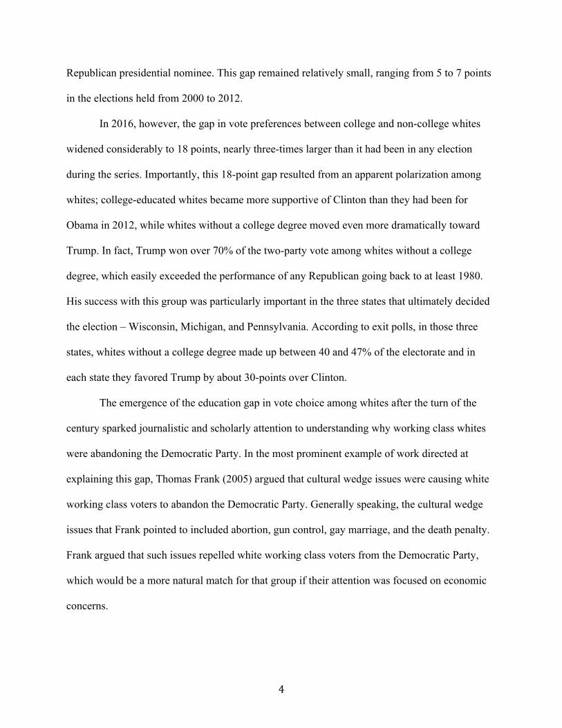
Figure 4 shows the relationship between a likely voter’s value on the racism and sexism

scales and his predicted favorability rating for each politician. These predictions were generated

from identical models to those analyzed above, except in this case we use the favorability rating

as the dependent variable rather than vote choice and we use OLS as our estimator rather than

probit. We re-scaled the favorability ratings so that they ranged from 0 (very unfavorable) to 1

(very favorable). The full results for these models are included in the Appendix. The patterns in

Figure 4 are quite striking, particularly for Republicans. Specifically, we find no statistically

significant relationship between either the racism or sexism scales and favorability ratings of

either John McCain or Mitt Romney. However, the pattern is quite strong for favorability ratings

of Donald Trump. In fact, people who score among the highest values of racism or sexism rate

Trump about twice as favorably as those with the lowest values on those scales, holding all other

variables in the model at their mean values. From this analysis, it certainly appears as though

support for the previous two Republican nominees was not affected by racism and sexism in the

same way that support for Trump was.

21

Interestingly, the patterns for Clinton and Obama’s favorability ratings are quite similar

to each other. While Obama had higher favorability ratings than Clinton across the board, both

were related to sexism and racism in similar ways. Yet, the 2016 election featured the only

Figure 4: Predicted favorability ratings based on values of racism and sexism

Note: Predicted ratings while holding all other variables in model at their mean values. Vertical lines represent 95% confidence intervals.

22

pairing of candidate whose favorability ratings were both affected by peoples’ levels of racism

and sexism.

As an additional test of whether 2016 was unique, we draw on a survey of likely voters

conducted in New Hampshire in October 2016.4 In that survey, we asked respondents not only

who they would support in the 2016 election, but we also asked them to recall who they voted

for in 2012. While the questionnaire for this survey did not include the racism battery or the

question related to economic dissatisfaction, it did include the same four hostile sexism items

from our national survey. Using this data, we estimated two vote choice models – one for

whether the likely voter said they were going to vote for Trump or Clinton in 2016, and a second

for whether the likely voter said they voted for Romney or Obama in 2012. As with our other

models, we include controls for partisanship, ideology, gender, age, and education. We exclude a

control for race in this model since nearly all of the likely voters in New Hampshire were white.

Table 3 shows the results from the two vote choice models. We are particularly interested

in comparing the coefficients for the hostile sexism scale. While hostile sexism does have a

positive coefficient for the 2012 model, the coefficient is not statistically significant and the size

of the effect is less than one-fourth as large as what it is in the 2016 vote choice model. A

difference of coefficients test indicates that we can be highly confident (p < .01) that the

relationship between sexism and vote choice in 2016 was larger than it was for the 2012 vote.

Figure 5 shows how the predicted probability of voting for Trump and Romney was affected by

increasing sexism while holding the other variables in the model at their mean values. Based on

this analysis, it does appear that sexism played a much more important role in affecting the 2016

vote than it did for 2012.

4The field dates for this survey were October 17 – October 21, 2016. The survey was also conducted by YouGov using a similar methodology as that for the national survey we analyze. Additional details are provided in the Appendix.

23

Table 3: Probit estimates of factors affecting two-party vote for Republican presidential candidate in New Hampshire in 2012 and 2016 2012 Presidential Vote 2016 Presidential Vote Hostile sexism scale 0.732 3.132 (0.486) (0.637)** Ideology 3.145 3.370 (0.689)** (0.602)** 7 point Party ID 4.056 3.670 (0.599)** (0.525)** Female -0.116 0.175 (0.198) (0.204) Age 30-54 0.241 -0.222 (0.426) (0.452) Age 55+ 0.035 -0.188 (0.434) (0.445) College degree -0.050 -0.277 (0.195) (0.210) Income <$40k -0.116 0.558 (0.311) (0.322) Income $40k - $100k -0.467 -0.059 (0.250) (0.337) Income >$100k -0.244 0.228 (0.279) (0.370) Constant -3.766 -5.061 (0.578)** (0.611)** Adjusted Count R2 0.768 0.789 N 554 551 Note: Entries are probit coefficients with standard errors in parentheses. * p<.05, ** p<.01.

24

Ideally, we would have survey data from previous election cycles that would allow us to

make cross-election comparisons in terms of the importance of our racism and sexism scales on

the presidential vote. Nevertheless, the analysis of the survey data from New Hampshire and the

national data on favorability ratings for current and past nominees provides a relatively strong

indication that racism and sexism were more important in 2016 than they had been in previous

elections (see also Tessler 2016).

Can Sexism and Racism Explain the Education Gap?

So far, we have demonstrated that sexism and racism were strongly associated with

presidential vote choice in 2016. We have also provided some evidence to support the notion that

Figure 5: Predicted probability of voting for Republican nominee in 2012 and 2016 based on values of sexism

Note: Predicted probabilities based on the models in Table 3 while holding all other variables in model at their mean values. Vertical lines represent 95% confidence intervals.

25

these associations were uniquely potent in 2016 compared to recent presidential elections. But

can racism and sexism help to explain the record gap in voting behavior between college and

non-college whites in 2016?

The 2016 exit polls found that 52% of the two-party vote among whites with at least a

college degree went to Trump, while Trump won 71% of the two-party vote among whites

without a college degree. This amounts to a 19-point gap in the vote choices of whites based on

education. In the pre-election survey that we analyze in this paper, we found a 22-point gap in

the vote choices of college and non-college educated whites. This gap is reflected by the

coefficient on gender in the first column of Table 4. This table presents a series of simple OLS

models for white likely voters in our sample. The aim is to examine how controlling for each of

our key variables might help to explain the education gap among whites. Thus, the greater a

reduction in the size of the coefficient for the college variable in a particular model, the more

those variables help to account for the gap.5

Table 4: The college gap among white likely voters in the two-party vote for Trump Controlling for… Base

Gap Econ.

Satisfaction

Sexism

Racism Racism &

Sexism College degree -0.221 -0.176 -0.099 -0.108 -0.071 (0.042)** (0.042)** (0.036)** (0.032)** (0.031)* Economic dissatisfaction 0.370 (0.078)** Hostile sexism scale 1.097 0.641 (0.054)** (0.070)** Racism scale 1.481 1.029 (0.058)** (0.087)** Constant 0.636 0.394 0.115 -0.053 -0.147 (0.027) (0.055) (0.038) (0.036) (0.034) R2 0.04 0.09 0.37 0.42 0.50 N 800 796 800 800 800 Note: Entries are OLS coefficients with standard errors in parentheses. * p<.05, **p<.01.

5 We note here that controlling for a respondent’s income does not affect the size of the education gap at all.

26

The second column in Table 4 adds our variable capturing respondents’ levels of

economic dissatisfaction. As we saw in our previous vote choice models, this variable is

statistically significant and clearly important. However, controlling for economic dissatisfaction

only reduces the size of the education gap from 22 points to 18 points. Thus, economic

dissatisfaction does not account for most of this gap. In the third and fourth columns, we add our

sexism and racism scales, respectively. Adding each of those variables individually to the model

results in a much larger reduction in the education gap. In fact, controlling for racism or sexism

reduces the size of the education gap by more than half.

The final model in Table 4 includes both the scales for racism and sexism to see what

combined effect both items have on reducing the education gap among whites. When we control

for both an individual’s attitudes on racism and sexism, the college gap drops to 7-points; this is

less than one-third of the size of the original education gap among whites. It is perhaps worth

remembering here that the previous four presidential elections witnessed a college vote choice

gap among whites of between 5 and 7 percentage points. Thus, controlling for racism and sexism

effectively restores the education gap among whites to what it had been in every election since

2000.

Conclusion

The 2016 campaign witnessed a dramatic polarization in the vote choices of whites based

on education. In this paper, we have demonstrated that very little of this gap can be explained by

the economic difficulties faced by less educated whites. Rather, most of the divide appears to be

the result of racism and sexism in the electorate, especially among whites without college

degrees. Sexism and racism were powerful forces in structuring the 2016 presidential vote, even

27

after controlling for partisanship and ideology. Of course, it would be misguided to seek an

understanding of Trump’s success in the 2016 presidential election through any single lens. Yet,

in a campaign that was marked by exceptionally explicit rhetoric on race and gender, it is

perhaps unsurprising to find that voters’ attitudes on race and sex were so important in

determining their vote choices.

How might have racism and sexism mattered for affecting the final outcome? One way to

approach this question is to consider how the vote might have differed if whites without college

degrees had the same average levels on the racism and sexism scales as whites who have college

degrees. If we make such an adjustment in our data, we find that Trump’s total two-party vote

share would have declined by 2 points.6 In other words, if non-college educated whites became

somewhat more progressive in their attitudes toward racism and sexism so that they matched

those of college educated whites, Clinton would have won the popular vote by 4 points instead of

2 points. Given the narrowness with which Clinton lost states like Wisconsin, Michigan,

Pennsylvania, and Florida, such a shift could have had a dramatic effect in terms of the Electoral

College outcome.

Whether the 2016 election will simply be an aberration or the beginning of a trend

remains to be seen. However, there is reason to think that Trump’s strategy of using explicitly

racist and sexist appeals to win over white voters may be followed again by candidates in future

elections. After all, Valentino et al. (2016) show that there is no longer a price to be paid by

politicians who make such explicit appeals. Explicit racist and sexist appeals appeared to cost

Trump some votes from more educated whites, but it may have won him even more support

6To create this calculation, we first estimate the vote choice model in Table 2. We then generate vote predictions for each respondent based on their values on the variables in the model. The next step is to reduce the racism and sexism scale measure for each white respondent without a college degree by a magnitude equal to the mean difference between college and non-college whites (e.g. the values in Table 1) and then create a second prediction based on those new values. The difference between the first prediction and the second is 2 points.

28

among whites with less education. If Republicans see little prospect of winning over racial or

ethnic minorities in the near future, they have two choices – moderate their appeals in order to

restore their advantage among more educated white voters (even if it costs them some votes

among less educated whites) or repeat the Trump strategy to maximize their support among less

educated whites (even at the expense of winning large margins among college educated whites).

As the norms governing political rhetoric appear to have largely been shattered in 2016, the latter

strategy is at least as plausible as the former, and that may have significant consequences for the

stability of American democracy.

29

References Bartels, Larry M. "What’s the Matter with What’s the Matter with Kansas?." Quarterly Journal

of Political Science 1, no. 2 (2006): 201-226. Bos, Angela L., Monica C. Schneider, and Brittany L. Utz. 2017. “Navigating the Political

Labyrinth: Gender Stereotypes and Prejudice in U.S. Elections.” In APA Handbook of the Psychology of Women, Cheryl Travis and Jackie White, Editors.

Brady, David, Benjamin Sosnaud, and Steven M. Frenk. "The shifting and diverging white

working class in US presidential elections, 1972–2004." Social Science Research 38, no. 1 (2009): 118-133.

Claassen, Ryan L., and John Barry Ryan. "Social Desirability, Hidden Biases, and Support for

Hillary Clinton." PS: Political Science & Politics 49, no. 4 (2016): 730-735. DeSante, Christopher D. and Candis W. Smith. 2016. “The Two Dimensions of Whites’ Racial

Attitudes, or: The New New Racism.” Working paper. Dolan, Kathleen. "Gender Stereotypes, Candidate Evaluations, and Voting for Women

Candidates What Really Matters?." Political Research Quarterly 67, no. 1 (2014): 96-107.

Frank, Thomas. What's the matter with Kansas?: how conservatives won the heart of America.

Macmillan, 2007. Glick, Peter, and Susan T. Fiske. "The ambivalent sexism inventory: Differentiating hostile and

benevolent sexism." Journal of personality and social psychology 70, no. 3 (1996): 491. Glick, Peter, Maria Lameiras, and Yolanda Rodriguez Castro. "Education and Catholic

religiosity as predictors of hostile and benevolent sexism toward women and men." Sex Roles 47, no. 9-10 (2002): 433-441.

Hayes, Danny. "When gender and party collide: Stereotyping in candidate trait

attribution." Politics & Gender 7, no. 02 (2011): 133-165. Huddy, Leonie, and Nayda Terkildsen. "Gender stereotypes and the perception of male and

female candidates." American Journal of Political Science (1993): 119-147. Masket, Seth. “What’s the Matter With Kansas? aptly describes the 2016 election — but was

written in 2004”. Vox. (2016). Url: http://www.vox.com/mischiefs-of-faction/2016/12/1/13807382/thomas-frank-kansas-2016-election

McGill, Andrew. “America’s Educational Divide Put Trump in the White House.” The Atlantic.

November 27, 2016. URL:

30

http://www.theatlantic.com/politics/archive/2016/11/education-put-donald-trump-in-the-white-house/508703/

Mendelberg, Tali. The race card: Campaign strategy, implicit messages, and the norm of

equality. Princeton University Press, 2001. Neville, Helen A., Roderick L. Lilly, Georgia Duran, Richard M. Lee, and LaVonne Browne.

"Construction and initial validation of the Color-Blind Racial Attitudes Scale (CoBRAS)." Journal of Counseling Psychology 47, no. 1 (2000): 59.

Pearson, Kathryn, and Eric McGhee. "What It Takes to Win: Questioning" Gender Neutral"

Outcomes in US House Elections." Politics & Gender 9, no. 4 (2013): 439. Porter, Eduardo. “Where Were Trump’s Votes? Where the Jobs Weren’t.” New York Times (Dec.

14, 2016): B1. Poteat, V. Paul, and Lisa B. Spanierman. "Further validation of the Psychosocial Costs of

Racism to Whites Scale among employed adults." The Counseling Psychologist 36, no. 6 (2008): 871-894.

Schuman, Howard, Steeh Charlotte, Bobo Lawrence, and Krysan Maria. "Racial Attitudes in

America: Trends and Interpretations." Cambridge, MA: Harvard (1997). Silver, Nate. “Education, Not Income, Predicted Who Would Vote for Trump.” FiveThirtyEight.

November 22, 2016. URL: http://fivethirtyeight.com/features/education-not-income-predicted-who-would-vote-for-trump/

Sniderman, Paul M., and Thomas Piazza. The Scar of Race Cambridge: Belknap/Harvard Univ.

Press (1993). Spanierman, Lisa B., and Mary J. Heppner. "Psychosocial Costs of Racism to Whites Scale

(PCRW): Construction and Initial Validation." Journal of Counseling Psychology 51, no. 2 (2004): 249.

Spanierman, Lisa B., V. Paul Poteat, Amanda M. Beer, and Patrick Ian Armstrong.

"Psychosocial costs of racism to whites: Exploring patterns through cluster analysis." Journal of Counseling Psychology 53, no. 4 (2006): 434.

Streb, Matthew J., Barbara Burrell, Brian Frederick, and Michael A. Genovese. "Social

desirability effects and support for a female American president." Public Opinion Quarterly 72, no. 1 (2008): 76-89.

Tankersly, Jim. “How Trump won: The revenge of working-class whites.” Washington Post.

November 9, 2016. URL: https://www.washingtonpost.com/news/wonk/wp/2016/11/09/how-trump-won-the-revenge-of-working-class-whites/?utm_term=.fb255924d80b

31

Tesler, Michael. “Views about race mattered more in electing Trump than in electing Obama.”

Washington Post (Monkey Cage). November 22, 2016. URL: https://www.washingtonpost.com/news/monkey-cage/wp/2016/11/22/peoples-views-about-race-mattered-more-in-electing-trump-than-in-electing-obama

Valentino, Nicholas A., Vincent L. Hutchings, and Ismail K. White. "Cues that matter: How

political ads prime racial attitudes during campaigns." American Political Science Review 96, no. 01 (2002): 75-90.

Valentino, Nicholas A. Fabian G. Neuner, and L. Matthew Vandenbroek. “The Changing Norms

of Racial Political Rhetoric and the End of Racial Priming.” Working paper. URL: https://www.researchgate.net/publication/310230276_The_Changing_Norms_of_Racial_Political_Rhetoric_and_the_End_of_Racial_Priming

32

Appendix Table A1: Full model results for the analysis of favorability ratings (Figure 4)

Trump Romney McCain Clinton Obama Hostile sexism 0.292 0.013 -0.022 -0.185 -0.287 (0.052)** (0.057) (0.049) (0.036)** (0.039)** Racism scale 0.284 -0.037 -0.017 -0.264 -0.268 (0.059)** (0.071) (0.061) (0.059)** (0.050)** Ec. dissatisfaction 0.107 -0.139 -0.068 -0.161 -0.175 (0.040)** (0.043)** (0.039) (0.035)** (0.033)** Ideology 0.126 0.151 0.122 -0.102 -0.177 (0.046)** (0.056)** (0.049)* (0.047)* (0.039)** 7 point Party ID 0.443 0.175 0.080 -0.616 -0.629 (0.045)** (0.047)** (0.039)* (0.037)** (0.034)** Female -0.023 0.014 0.064 0.008 0.008 (0.021) (0.023) (0.020)** (0.018) (0.017) Age 30-54 0.057 -0.036 -0.013 -0.011 -0.033 (0.045) (0.050) (0.038) (0.042) (0.037) Age 55+ 0.099 -0.107 -0.039 -0.020 -0.068 (0.045)* (0.050)* (0.038) (0.043) (0.036) College degree -0.091 0.087 0.049 -0.006 0.011 (0.020)** (0.023)** (0.022)* (0.019) (0.020) Income <$40k -0.008 0.040 0.014 0.065 -0.000 (0.032) (0.036) (0.035) (0.026)* (0.029) Income $40-100k -0.022 -0.003 0.023 0.051 0.003 (0.029) (0.033) (0.034) (0.025)* (0.028) Income >$100k -0.065 0.032 0.061 0.100 0.023 (0.038) (0.041) (0.043) (0.031)** (0.033) White -0.009 0.095 0.028 0.020 0.014 (0.038) (0.040)* (0.042) (0.030) (0.034) Black -0.138 0.028 0.066 0.120 0.156 (0.046)** (0.048) (0.049) (0.036)** (0.040)** Hispanic -0.042 0.008 0.036 0.047 0.031 (0.043) (0.045) (0.048) (0.040) (0.041) Constant -0.194 0.279 0.285 0.948 1.215 (0.062)** (0.066)** (0.073)** (0.059)** (0.061)** R2 0.57 0.14 0.05 0.65 0.72 N 1,404 1,292 1,298 1,410 1,408