exploiting large-scale data analytics platforms with
TRANSCRIPT

Exploiting Large-scale Data Analytics Platforms with Accelerator
Hardware
A Dissertation Presented
by
Xiangyu Li
to
The Department of Electrical and Computer Engineering
in partial fulfillment of the requirements
for the degree of
Doctor of Philosophy
in
Computer Engineering
Northeastern University
Boston, Massachusetts
August 2018

ProQuest Number:
All rights reserved
INFORMATION TO ALL USERSThe quality of this reproduction is dependent upon the quality of the copy submitted.
In the unlikely event that the author did not send a complete manuscriptand there are missing pages, these will be noted. Also, if material had to be removed,
a note will indicate the deletion.
ProQuest
Published by ProQuest LLC ( ). Copyright of the Dissertation is held by the Author.
All rights reserved.This work is protected against unauthorized copying under Title 17, United States Code
Microform Edition © ProQuest LLC.
ProQuest LLC.789 East Eisenhower Parkway
P.O. Box 1346Ann Arbor, MI 48106 - 1346
10933920
10933920
2018

I would like to dedicate this dissertation to my lovely wife, Xingyan Xu. I would also like to thank my
mother Li Li, and my father Shuyi Li for raising me and supporting me through to what I have
achieved today.
i

Contents
List of Figures iv
List of Tables vi
List of Acronyms vii
Acknowledgments viii
Abstract of the Dissertation ix
1 Introduction 11.1 Machine Learning . . . . . . . . . . . . . . . . . . . . . . . . . . . . . . . . . . . 11.2 Parallel Processors . . . . . . . . . . . . . . . . . . . . . . . . . . . . . . . . . . 21.3 Distributed Systems . . . . . . . . . . . . . . . . . . . . . . . . . . . . . . . . . . 41.4 Parallelism in ML Algorithms . . . . . . . . . . . . . . . . . . . . . . . . . . . . 51.5 Motivation . . . . . . . . . . . . . . . . . . . . . . . . . . . . . . . . . . . . . . . 61.6 Challenges . . . . . . . . . . . . . . . . . . . . . . . . . . . . . . . . . . . . . . . 8
1.6.1 Maintaining a simple frontend interface for a powerful GPU backend . . . 81.6.2 Targeted Workloads . . . . . . . . . . . . . . . . . . . . . . . . . . . . . 9
1.7 Contributions of the Thesis . . . . . . . . . . . . . . . . . . . . . . . . . . . . . . 101.8 Organization of Thesis . . . . . . . . . . . . . . . . . . . . . . . . . . . . . . . . 10
2 Background 122.1 GPUs . . . . . . . . . . . . . . . . . . . . . . . . . . . . . . . . . . . . . . . . . 12
2.1.1 GPU Architectures . . . . . . . . . . . . . . . . . . . . . . . . . . . . . . 132.1.2 CUDA . . . . . . . . . . . . . . . . . . . . . . . . . . . . . . . . . . . . 142.1.3 OpenCL . . . . . . . . . . . . . . . . . . . . . . . . . . . . . . . . . . . . 16
2.2 Distributed Systems . . . . . . . . . . . . . . . . . . . . . . . . . . . . . . . . . . 172.2.1 MapReduce . . . . . . . . . . . . . . . . . . . . . . . . . . . . . . . . . . 182.2.2 Hadoop . . . . . . . . . . . . . . . . . . . . . . . . . . . . . . . . . . . . 202.2.3 Spark . . . . . . . . . . . . . . . . . . . . . . . . . . . . . . . . . . . . . 21
ii

3 Related Work 243.1 MapReduce-based Distributed Systems with GPUs . . . . . . . . . . . . . . . . . 24
3.1.1 Stand-alone Frameworks . . . . . . . . . . . . . . . . . . . . . . . . . . . 263.1.2 Hadoop/Spark Compatible Frameworks . . . . . . . . . . . . . . . . . . . 28
3.2 Preliminary Work . . . . . . . . . . . . . . . . . . . . . . . . . . . . . . . . . . . 303.2.1 Mahout . . . . . . . . . . . . . . . . . . . . . . . . . . . . . . . . . . . . 313.2.2 PairwiseSimilarity Job in Mahout . . . . . . . . . . . . . . . . . . . . . . 323.2.3 PairwiseSimilarity Job in HadoopCL . . . . . . . . . . . . . . . . . . . . 333.2.4 HadoopCL Cooperative Model . . . . . . . . . . . . . . . . . . . . . . . . 353.2.5 Conclusion . . . . . . . . . . . . . . . . . . . . . . . . . . . . . . . . . . 36
4 Enabling Accelerators on Spark System 374.1 GPUEnabler . . . . . . . . . . . . . . . . . . . . . . . . . . . . . . . . . . . . . . 37
4.1.1 GPUEnabler Program Example . . . . . . . . . . . . . . . . . . . . . . . 394.2 Improvements to GPUEnabler . . . . . . . . . . . . . . . . . . . . . . . . . . . . 404.3 Performance Evaluation . . . . . . . . . . . . . . . . . . . . . . . . . . . . . . . . 43
4.3.1 Machine Learning Benchmarks . . . . . . . . . . . . . . . . . . . . . . . 434.3.2 Experimental Setup . . . . . . . . . . . . . . . . . . . . . . . . . . . . . . 514.3.3 Performance versus input data sizes . . . . . . . . . . . . . . . . . . . . . 51
5 Sparkculator 565.1 User Interface . . . . . . . . . . . . . . . . . . . . . . . . . . . . . . . . . . . . . 575.2 Sparkculator ML Library . . . . . . . . . . . . . . . . . . . . . . . . . . . . . . . 575.3 Developer Interface . . . . . . . . . . . . . . . . . . . . . . . . . . . . . . . . . . 58
5.3.1 mapCUDA . . . . . . . . . . . . . . . . . . . . . . . . . . . . . . . . . . 585.3.2 SparkcuFunc . . . . . . . . . . . . . . . . . . . . . . . . . . . . . . . . . 59
5.4 Sparkculator Core . . . . . . . . . . . . . . . . . . . . . . . . . . . . . . . . . . . 605.4.1 Offloading CUDA Functions to GPUs . . . . . . . . . . . . . . . . . . . . 605.4.2 Offloading Spark Data to GPUs . . . . . . . . . . . . . . . . . . . . . . . 605.4.3 Buffer Caching and Lazy Evaluation . . . . . . . . . . . . . . . . . . . . . 61
5.5 Performance Evaluation . . . . . . . . . . . . . . . . . . . . . . . . . . . . . . . . 635.5.1 Experimental Setup . . . . . . . . . . . . . . . . . . . . . . . . . . . . . . 645.5.2 Benchmarks and Datasets . . . . . . . . . . . . . . . . . . . . . . . . . . 645.5.3 Overall performance and scalability . . . . . . . . . . . . . . . . . . . . . 655.5.4 Execution Time Breakdown . . . . . . . . . . . . . . . . . . . . . . . . . 66
6 Conclusion 696.1 Future Research Directions . . . . . . . . . . . . . . . . . . . . . . . . . . . . . . 70
iii

List of Figures
1.1 Supervised and Unsupervised Learning. . . . . . . . . . . . . . . . . . . . . . . . 31.2 Distributing ML Workload to CPUs and GPUs on Multiple Nodes. . . . . . . . . . 6
2.1 Tesla K40 GPU Architecture. . . . . . . . . . . . . . . . . . . . . . . . . . . . . . 132.2 CUDA Execution Model and Memory Hierarchy. . . . . . . . . . . . . . . . . . . 152.3 OpenCL Execution and Memory Model . . . . . . . . . . . . . . . . . . . . . . . 162.4 MapReudce Programming Model Overview. . . . . . . . . . . . . . . . . . . . . . 182.5 Counting Occurrences of Words in a Large Text File using MapReduce. . . . . . . 192.6 Hadoop Framework. . . . . . . . . . . . . . . . . . . . . . . . . . . . . . . . . . 202.7 Spark Framework. . . . . . . . . . . . . . . . . . . . . . . . . . . . . . . . . . . . 212.8 Lineage graph for logistic regression, different data structures are represented with
different shapes . . . . . . . . . . . . . . . . . . . . . . . . . . . . . . . . . . . . 23
3.1 An example of Mahout processing a movie ratings dataset. . . . . . . . . . . . . . 313.2 The PairwiseSimilarity job in Hadoop. . . . . . . . . . . . . . . . . . . . . . . . . 323.3 Data Format in Mahout and HadoopCL. . . . . . . . . . . . . . . . . . . . . . . . 333.4 HadoopCL vs. cooperative HadoopCL. . . . . . . . . . . . . . . . . . . . . . . . 34
4.1 An overview of GPUEnabler. . . . . . . . . . . . . . . . . . . . . . . . . . . . . . 384.3 K-Means’ Performance on Synthetic Datasets. . . . . . . . . . . . . . . . . . . . . 524.4 Logistic Regression’s Performance on Synthetic Datasets. . . . . . . . . . . . . . . 544.5 Page Rank’s Performance on Synthetic Datasets. . . . . . . . . . . . . . . . . . . 55
5.1 The Sparkculator software stack. The gray boxes are the novel components . . . . 575.2 Input, broadcast, and output SparkcuBuffers, an arrow indicates a data transfer
direction from one memory space to another. . . . . . . . . . . . . . . . . . . . . 625.3 Lineage graph for 2 iterations of logistic regression in Sparkculator, a Sparkculator
buffer contains at most four different types of memory: RDD, CPU off-heap, GPUglobal, and GPU shared . . . . . . . . . . . . . . . . . . . . . . . . . . . . . . . . 63
5.4 Sparkculator’s overall speedup for each benchmark running on 2, 4, and 8 workernodes. . . . . . . . . . . . . . . . . . . . . . . . . . . . . . . . . . . . . . . . . . 65
5.5 Speedup achieved when using 4 and 8 nodes versus 2 nodes on each platform. . . . 665.6 CPU and GPU execution time breakdown for LR on 2 worker nodes versus 4 worker
nodes, across 3 iterations. . . . . . . . . . . . . . . . . . . . . . . . . . . . . . . . 67
iv

5.7 CPU and GPU execution time breakdown for KMeans, Fuzzy and GA on 2 workernodes, across 3 iterations. . . . . . . . . . . . . . . . . . . . . . . . . . . . . . . . 68
v
List of Tables
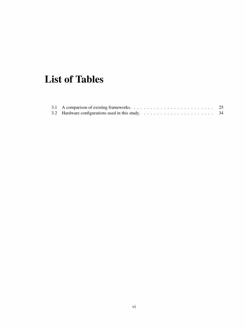
3.1 A comparison of existing frameworks. . . . . . . . . . . . . . . . . . . . . . . . . 253.2 Hardware configurations used in this study. . . . . . . . . . . . . . . . . . . . . . 34
vi
List of Acronyms
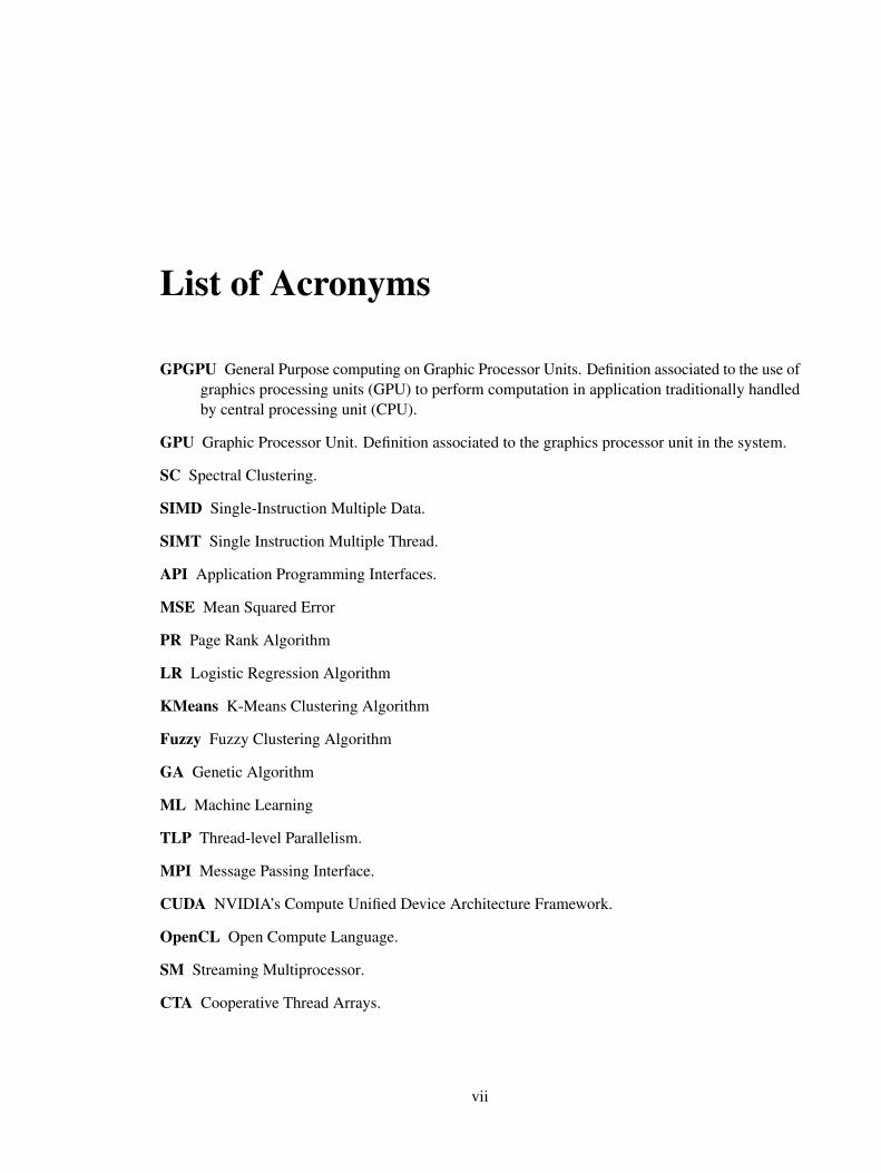
GPGPU General Purpose computing on Graphic Processor Units. Definition associated to the use ofgraphics processing units (GPU) to perform computation in application traditionally handledby central processing unit (CPU).
GPU Graphic Processor Unit. Definition associated to the graphics processor unit in the system.
SC Spectral Clustering.
SIMD Single-Instruction Multiple Data.
SIMT Single Instruction Multiple Thread.
API Application Programming Interfaces.
MSE Mean Squared Error
PR Page Rank Algorithm
LR Logistic Regression Algorithm
KMeans K-Means Clustering Algorithm
Fuzzy Fuzzy Clustering Algorithm
GA Genetic Algorithm
ML Machine Learning
TLP Thread-level Parallelism.
MPI Message Passing Interface.
CUDA NVIDIA’s Compute Unified Device Architecture Framework.
OpenCL Open Compute Language.
SM Streaming Multiprocessor.
CTA Cooperative Thread Arrays.
vii
Acknowledgments
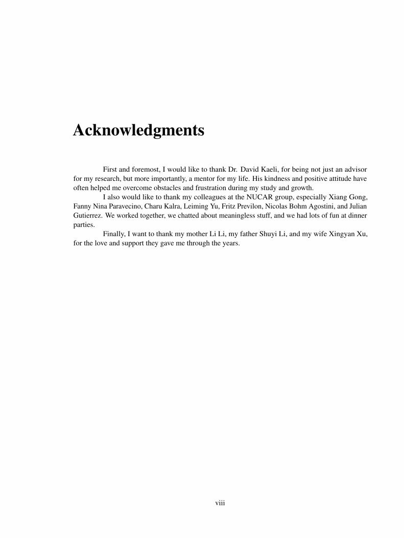
First and foremost, I would like to thank Dr. David Kaeli, for being not just an advisorfor my research, but more importantly, a mentor for my life. His kindness and positive attitude haveoften helped me overcome obstacles and frustration during my study and growth.
I also would like to thank my colleagues at the NUCAR group, especially Xiang Gong,Fanny Nina Paravecino, Charu Kalra, Leiming Yu, Fritz Previlon, Nicolas Bohm Agostini, and JulianGutierrez. We worked together, we chatted about meaningless stuff, and we had lots of fun at dinnerparties.
Finally, I want to thank my mother Li Li, my father Shuyi Li, and my wife Xingyan Xu,for the love and support they gave me through the years.
viii
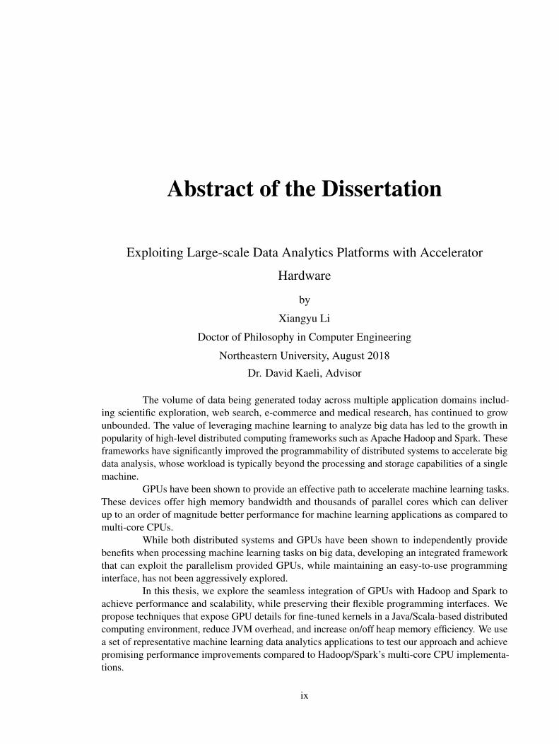
Abstract of the Dissertation
Exploiting Large-scale Data Analytics Platforms with Accelerator
Hardware
by
Xiangyu Li
Doctor of Philosophy in Computer Engineering
Northeastern University, August 2018
Dr. David Kaeli, Advisor
The volume of data being generated today across multiple application domains includ-ing scientific exploration, web search, e-commerce and medical research, has continued to growunbounded. The value of leveraging machine learning to analyze big data has led to the growth inpopularity of high-level distributed computing frameworks such as Apache Hadoop and Spark. Theseframeworks have significantly improved the programmability of distributed systems to accelerate bigdata analysis, whose workload is typically beyond the processing and storage capabilities of a singlemachine.
GPUs have been shown to provide an effective path to accelerate machine learning tasks.These devices offer high memory bandwidth and thousands of parallel cores which can deliverup to an order of magnitude better performance for machine learning applications as compared tomulti-core CPUs.
While both distributed systems and GPUs have been shown to independently providebenefits when processing machine learning tasks on big data, developing an integrated frameworkthat can exploit the parallelism provided GPUs, while maintaining an easy-to-use programminginterface, has not been aggressively explored.
In this thesis, we explore the seamless integration of GPUs with Hadoop and Spark toachieve performance and scalability, while preserving their flexible programming interfaces. Wepropose techniques that expose GPU details for fine-tuned kernels in a Java/Scala-based distributedcomputing environment, reduce JVM overhead, and increase on/off heap memory efficiency. We usea set of representative machine learning data analytics applications to test our approach and achievepromising performance improvements compared to Hadoop/Spark’s multi-core CPU implementa-tions.
ix

x

Chapter 1
Introduction
The unprecedented growth of data over the past decade can be attributed to many factors.
Data collection devices that have increased precision and resolution, have become cheaper and
easier to use, generating an ever-increasing amount of scientific data. Websites that let users share
self-created content such as Facebook, Youtube, and Instagram are collecting petabytes of social data
on a daily basis [1].
Given this growth in data, Machine Learning (ML) techniques have emerged as an im-
portant class of algorithms, since they excel in a diverse set of data analysis tasks. A wide range
of applications have been developed in a number of domains, including medical diagnostics, web
search, online advertising, product recommendations, and computer vision. A general trend is that
datasets are getting larger and more complex, and accordingly, ML models are getting more and
more complicated. These models demand a rapidly growing amount of computational power, which
presents a number of challenges to system software and hardware designers.
To frame the scope of this thesis, we begin with a discussion on the technologies that
we plan to impact in this thesis: i) machine Learning workloads, and ii) parallel processing and
distributed systems.
1.1 Machine Learning
Machine Learning refers to a very large set of algorithms and tools used to understand data,
discovering patterns in the data, and predicting future outcomes with the existing data. There are two
major classes of machine learning algorithms: i) supervised learning, and ii) unsupervised learning.
1

CHAPTER 1. INTRODUCTION
In supervised learning, the training dataset consists of n pairs of (xi, yi), i = 1, ..., n,
where xi ∈ Rd and yi ∈ R1. The values in xi are called input variables, and yi is called an output
variable. The goal is to find a hypothesis function f that maps the input to the output, so that we
can use yi = f(xi) to approximate the output variable yi for all n input instances. This mapping can
then be used for predicting the output for a new input instance. The process of finding the hypothesis
function f is called training.
Figure 1.1a shows an example of training a linear model that predicts housing prices (the
output variable) based on the number of rooms in the house (the input variable). The black dots
represent the training dataset, and the line going through them is the model trained from the dataset,
which can be used to predict the housing price for a new input instance (e.g., the price of a house
with 4 rooms.) In this example, the model is a set of parameters defined by a vector w ∈ Rd, and the
price prediction for a new input instance x is wTx. Training an ML model can be formulated into
solving an optimization problem in the following form:
arg minwg(w) =1
n
n∑i=1
hi(w) (1.1)
The goal is to find the vector w that minimizes the sum of objective functions hi(w) for each data
point i. The objective function hi(w) characterizes how well the model w predicts the outcome for
the i-th data point.
In unsupervised learning, the training dataset contains only the input variables — there
are no output variables that supervise and guide the direction of the training process. The goal is to
find relationships among the input instances and identify interesting patterns and hidden structures
in the data. A typical example is to divide a set of data points into multiple groups, with the goal
of minimizing the distance among the data points within the same group, while maximizing the
inter-group distances. Figure 1.1b shows an example where a dataset is divided into three groups
using an unsupervised clustering algorithm; each group is denoted with a unique marker.
1.2 Parallel Processors
It has been almost two decades since the end of an era when a microprocessor designer
could improve a CPU’s performance by just increasing the clock speed. Thermal and power
technology had not been able to keep up with the heat generated as we increase CPU clock frequencies.
Multi-core processors have become the new normal, and the core count has increased dramatically;
2

CHAPTER 1. INTRODUCTION
4 5 6 7 8 9Average Number of Rooms per Dwelling
0
10
20
30
40
50
Med
ian
Price
($10
00s)
(a) Training a Linear Model to Predict Housing Price.
0 2 4 6 8 10 12X2
0
2
4
6
8
10
12
X1(b) Clustering a Dataset into 3 Groups.
Figure 1.1: Supervised and Unsupervised Learning.
the recent Intel i9 and AMD Threadripper CPUs both are equipped with 16 cores on a single chip.
A CPU core packs powerful ALUs and sophisticated control units, enhancing its ability to carry
out complicated tasks. However, it is not a trivial task to fully utilize the combined power of all
cores to deliver a high overall throughput. Developers need to rewrite the program by dividing an
originally single-threaded task into multiple independent tasks that can be assigned to multiple cores
for parallel execution.
In contrast to the task-level parallelism offered by multi-core CPUs, Graphics Processing
Units (GPUs) exploit thread-level parallelism in an application. Initially designed to render millions
of pixels at the same time, GPUs devote most of its die area and transistors to a large number of
light-weight computing cores (threads) and high-bandwidth memory, instead of sophisticated control
units in CPUs. GPUs adopt a single instruction multiple data (SIMD) execution model that uses
massive threads to execute a single instruction over thousands of data points in parallel, resulting
in extremely high computational and memory throughput. Constrained by the simplified control
units design, a group of 32 threads (called a warp) shares the same control logic on a GPU streaming
multiprocessor, resulting in poor performance when threads within a warp diverge in their execution
paths. This presents challenges to developers as they need to redesign their algorithms in a way
that avoids thread divergence as much as possible. Parallel programming frameworks, such as
Compute Unified Device Architecture (CUDA) and Open Computing Language (OpenCL), have
3

CHAPTER 1. INTRODUCTION
been introduced in the software community that help developers offload the parallel portion of their
algorithms to GPUs with kernel programs written in high-level languages.
1.3 Distributed Systems
While we have witnessed single system performance grow through increasing CPU through-
put and integrating accelerated co-processors, including GPUs and FPGAs, scaling out the system by
distributing the data and tasks to thousands of worker nodes has become increasingly popular. This
is because the storage and computing requirements of big data analytics workloads far exceed the
throughput available on a single system.
A number of distributed programming models have been proposed to meet the demands
of big data analytics tasks [2, 3, 4], among which, the MapReduce programming model is the most
widely-used framework for mapping work to a distributed system. The popularity of MapReduce has
grown based on its ease of use, especially in terms of programmability. It provides a simple interface
— map and reduce — for users to define in order to express their algorithms. Other distributed
systems related tasks, such as data partitioning, task scheduling, and fault tolerance, are all taken care
of by the MapReduce framework. Apache Hadoop [5] is one of the early adopters of the MapReduce
model, and has become widely used in both industry and academia. Hadoop significantly simplifies
distributed data analytic tasks, but its performance suffers from I/O bottlenecks, as it stores all the
intermediate data in secondary storage (i.e., disks). With DRAM getting cheaper and larger, a recent
trend in distributed computing is the use of memory to cache intermediate data during computations
to avoid the I/O overhead.
Apache Spark [6] is an open-source framework that is based on the MapReduce program-
ming model and the Hadoop File System (HDFS). Spark favors in-memory processing over I/O
operations. Spark is designed to benefit machine learning algorithms that iteratively update their pa-
rameters. Spark provides an in-memory processing model to allow iterative applications to read/write
frequently accessed data with low latency, until the computation converges. This class of computation
highlights Spark’s attractive benefits as compared to Hadoop. Another improvement of Spark over
Hadoop is its increased programmability; in addition to continued support of map and reduce
functions, Spark provides a wide range of data transformation APIs such as filter, sortByKey,
and reduceByKey. Spark is written in Scala [7], a functional programming language that makes
it much easier for users to describe their parallel tasks in a straightforward fashion. Because Scala
code compiles to Java bytecode and runs on a Java Virtual Machine (JVM), users can use the large
4

CHAPTER 1. INTRODUCTION
collection of existing Java libraries in Spark, significantly reducing development time. In addition,
Scala provides a clean function literal passing interface. This feature plays an important role in
Spark’s ability to build lineage graphs, in order to improve memory efficiency and ensure fault
tolerance by using in-memory data recovery.
1.4 Parallelism in ML Algorithms
In this section, we consider the parallelism present in ML algorithms, making them good
candidates to be executed on parallel processors and distributed systems. In supervised learning,
our goal is to minimize the objective function in 1.1. We use the most commonly-used objective —
minimizing mean squared error (MSE) — as an example to demonstrate how to deploy a typical ML
algorithm on a parallel platform. Let ei = yi − fw(xi) represent the ith residual — the difference
between the real and predicted value for the ith data point, we aim to find a model w that minimizes
f(w), described in the following equation:
f(w) =1
n
n∑i=1
ei2 (1.2)
To solve this problem, a heuristic approach is often used, in which we update the model w iteratively
until a certain stopping condition is met. Using the gradient descent method as an example, we start
with a randomly selected initial model w0 at iteration t = 0, and update the model w as follows until
it reaches convergence:
wt+1 = wt − αn∑
i=1
∂ei2 (1.3)
where ∂ei2 is the partial gradient of (yi − fw(xi))2
with respect to w, and α is a user-defined
constant scalar that specifies the step size in gradient descent. The partial gradient calculation in 1.3
is the computational bottleneck in most machine learning algorithms. Since the calculation for each
individual data point i is independent from each other, we can divide the workload into multiple
chunks and distribute a chunk per worker node, where it is further divided and assigned to multi-core
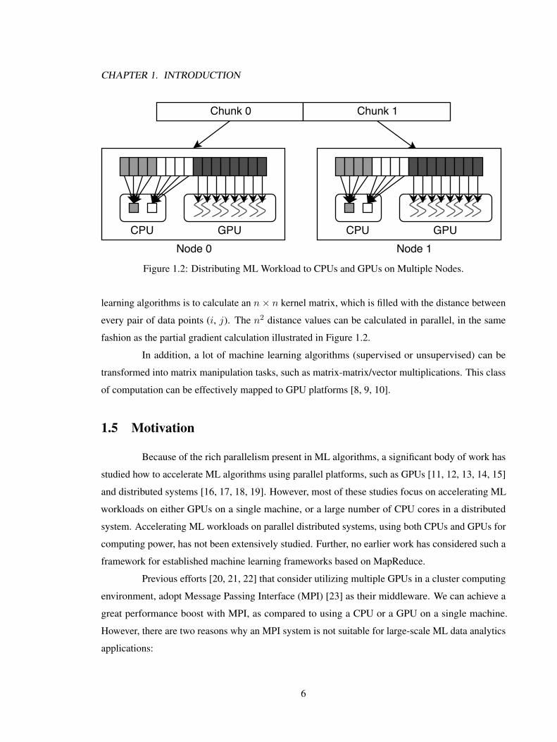
CPUs and many-core GPUs for an additional level of parallelism. Figure 1.2 illustrates how this
works on a 2-node cluster with a dual-core CPU and a GPU on each node. The input dataset is
split in two chunks and distributed to two worker nodes, where each CPU core carries out heavy
computation over multiple data points to exploit its task-level parallelism, and each GPU thread is
only assigned light-weight workload to utilize its thread-level parallelism. In unsupervised learning,
a similar parallel execution pattern is observed, e.g., an important component of various unsupervised
5
CHAPTER 1. INTRODUCTION
Figure 1.2: Distributing ML Workload to CPUs and GPUs on Multiple Nodes.
learning algorithms is to calculate an n× n kernel matrix, which is filled with the distance between
every pair of data points (i, j). The n2 distance values can be calculated in parallel, in the same
fashion as the partial gradient calculation illustrated in Figure 1.2.
In addition, a lot of machine learning algorithms (supervised or unsupervised) can be
transformed into matrix manipulation tasks, such as matrix-matrix/vector multiplications. This class
of computation can be effectively mapped to GPU platforms [8, 9, 10].
1.5 Motivation
Because of the rich parallelism present in ML algorithms, a significant body of work has
studied how to accelerate ML algorithms using parallel platforms, such as GPUs [11, 12, 13, 14, 15]
and distributed systems [16, 17, 18, 19]. However, most of these studies focus on accelerating ML
workloads on either GPUs on a single machine, or a large number of CPU cores in a distributed
system. Accelerating ML workloads on parallel distributed systems, using both CPUs and GPUs for
computing power, has not been extensively studied. Further, no earlier work has considered such a
framework for established machine learning frameworks based on MapReduce.
Previous efforts [20, 21, 22] that consider utilizing multiple GPUs in a cluster computing
environment, adopt Message Passing Interface (MPI) [23] as their middleware. We can achieve a
great performance boost with MPI, as compared to using a CPU or a GPU on a single machine.
However, there are two reasons why an MPI system is not suitable for large-scale ML data analytics
applications:
6
CHAPTER 1. INTRODUCTION
• The MPI standard is a low-level, explicit programming model. Developers need to manually
control and manage data partitioning, task scheduling, job synchronization, etc., to build
a working application. The development process is complicated and error-prone, which is
reasonable for designing domain-specific scientific computing applications that have long
software longevity, but unacceptable for ML data analytics applications that need constant
modification and a rapid development support.
• MPI is traditionally designed for executing scientific computing applications in a High Perfor-
mance Computing (HPC) environment with powerful and reliable computing components in a
supercomputer. In contrast, today’s data analytics applications more often run on hundreds of
commodity machines connected through ethernet in a cluster, where reliability issues arise
frequently since a machine can fail at any time, thus demanding much more fault tolerance
middleware versus what MPI can offer.
As a result, we would like to explore using high-level distributed computing frameworks — Hadoop
and Spark — as the foundation of a parallel and distributed ML framework. Hadoop and Spark have
gained great popularity in the past decade, mostly because of their ease of programming that simplifies
data analytics for large datasets, and reliable fault-tolerant mechanism. However, performance has
not been their strong suit. As discussed previously in Section 1.3, Hadoop’s performance is mostly
bottlenecked by its I/O performance as it relies on disks for intermediate data reads/writes and
checkpointing. Motivated to solve the issue in Hadoop, Spark was created. It allows the user to
indicate which data objects should be persisted in memory instead of on disks, thus significantly
improves performance as it eliminates the disk bottlenecks. Spark is among several software efforts
that strive to solve the I/O issues in the traditional Hadoop framework. Alongside these software
approaches, hardware efforts, such as replacing mechanical disks with solid state drives (SSDs),
increasing DRAM frequencies and capacities, and reducing network latency have also emerged.
These two forces combined produce a shift in the performance bottleneck of distributed systems,
from I/O, to computing and memory. In the foreseeable future, the lack of computing power will
become an increasingly prominent issue, with the I/O bottleneck being optimized away.
Driven by these recent advances in big data computation and cloud computing, this thesis
first investigates the use of GPUs in a Hadoop-based recommender system. We then move to Spark
and study existing work that utilizes the computational power of a GPU in a distributed system,
while providing an easy-to-use front-end interface. We study GPUEnabler [24], a GPU-enabled
Spark framework to identify the current limitations of the state-of-the-art GPU-enabled Spark toolset.
7
CHAPTER 1. INTRODUCTION
While we have learned a lot from this framework, GPUenabler has a number of fundamental design
issues that need to be addressed. We need to pursue further work to improve GPU performance and
scalability for machine learning workloads run on Spark. Our new framework is named Sparkculator,
which learns from the limitations of GPUEnabler, but is a completely new framework developed in
this thesis. We address a number of fundamental challenges in designing this framework, which we
outline next.
1.6 Challenges
1.6.1 Maintaining a simple frontend interface for a powerful GPU backend
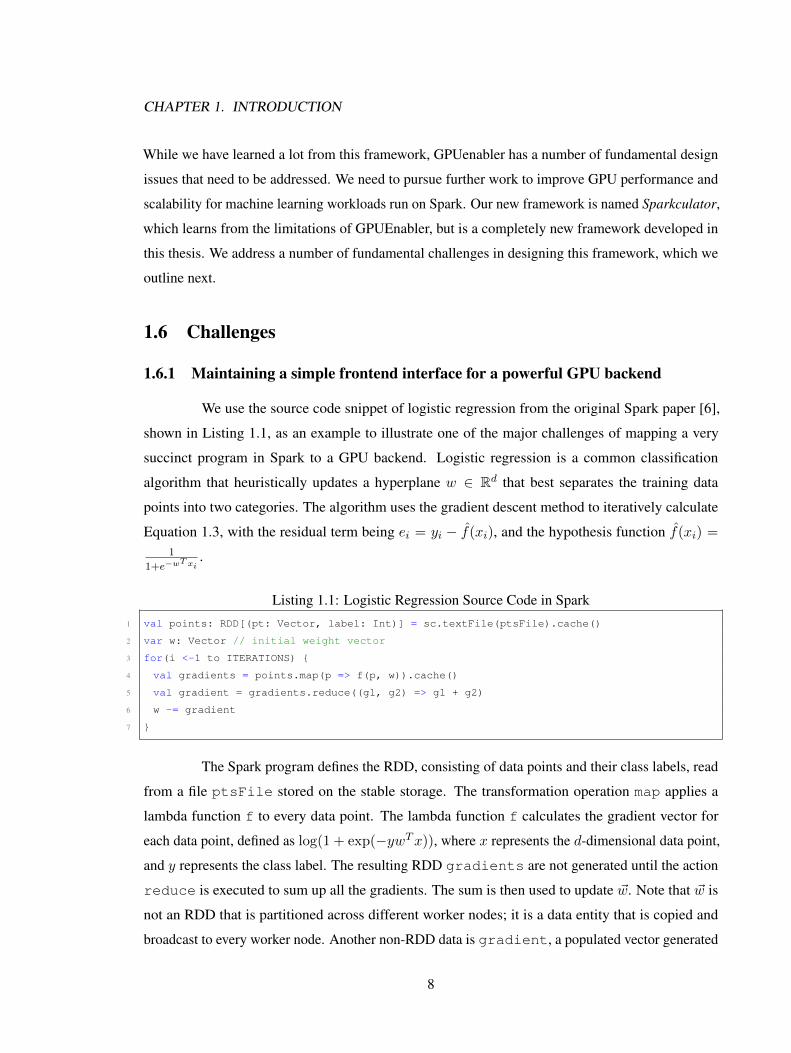
We use the source code snippet of logistic regression from the original Spark paper [6],
shown in Listing 1.1, as an example to illustrate one of the major challenges of mapping a very
succinct program in Spark to a GPU backend. Logistic regression is a common classification
algorithm that heuristically updates a hyperplane w ∈ Rd that best separates the training data
points into two categories. The algorithm uses the gradient descent method to iteratively calculate
Equation 1.3, with the residual term being ei = yi − f(xi), and the hypothesis function f(xi) =
1
1+e−wT xi.
Listing 1.1: Logistic Regression Source Code in Spark
1 val points: RDD[(pt: Vector, label: Int)] = sc.textFile(ptsFile).cache()
2 var w: Vector // initial weight vector
3 for(i <-1 to ITERATIONS)
4 val gradients = points.map(p => f(p, w)).cache()
5 val gradient = gradients.reduce((g1, g2) => g1 + g2)
6 w -= gradient
7
The Spark program defines the RDD, consisting of data points and their class labels, read
from a file ptsFile stored on the stable storage. The transformation operation map applies a
lambda function f to every data point. The lambda function f calculates the gradient vector for
each data point, defined as log(1 + exp(−ywTx)), where x represents the d-dimensional data point,
and y represents the class label. The resulting RDD gradients are not generated until the action
reduce is executed to sum up all the gradients. The sum is then used to update ~w. Note that ~w is
not an RDD that is partitioned across different worker nodes; it is a data entity that is copied and
broadcast to every worker node. Another non-RDD data is gradient, a populated vector generated
8
CHAPTER 1. INTRODUCTION
by the action reduce. For simplicity, we refer to non-RDD data resembling ptsFile as storage
data, ~w as broadcast data, and gradient as result data for the rest of the thesis.
There are two major challenges in designing a framework that enables GPU execution,
while maintaining a simple and clean programming interface: 1) function offloading, and 2) memory
management.
Function Offloading refers to transferring the compute-intensive portion of the Spark
operations to GPU(s) on each computing node. In Listing 1.1, the gradient calculation on line
4should be offloaded to the GPU. The Spark code uses Scala features such as anonymous function
and function literal passing, both of which are not supported in GPU programming languages such
as CUDA and OpenCL. For Spark’s RDD, broadcast, and result data, we need to create the GPU
counterparts, construct CUDA kernels with the corresponding parameters, and launch the kernels on
the GPU. Doing these with minimum code modification by the developer is not a trivial task.
Memory Management includes two major tasks: 1) transferring Spark’s data back and
forth between four different memory spaces: on-heap memory, off-heap memory, GPU’s global
memory, and GPU’s shared memory, 2) managing buffers in different memory spaces efficiently by
maximizing data re-use and minimizing buffer re-allocation. Scala runs on the Java Virtual Machine
(JVM), which wraps a raw data buffer alongside with the meta information and places it in its heap
area. The JVM keeps track of the object allocations on the heap to enable garbage collection —
a process that reclaims memory space automatically by deleting objects that are no longer in use.
For a GPU to access Java objects, such as points, we need to transform and transfer an iterator
of pts and label, together with their metadata (such as size and data type), from on-heap memory
to off-heap memory, and eventually to GPU’s global and shared memory. The second task is to
minimize the amount of data transferred between these memory space. Spark uses cache(), as shown
at line 1, to persist points in memory to reduce access latency. We need to build a GPU buffer
caching system that resembles Spark, to minimize the number of slow CPU-to-GPU data transfers
through PCI-e. In addition, we also need to implement a buffer recycling mechanism that reduce the
amount of GPU buffer allocation and de-allocation.
1.6.2 Targeted Workloads
In order to evaluate the programmability and the performance of the framework, we need
to find a set of real-world ML data analytics applications that are widely-used and represent a range
of different algorithmic characteristics. We also need to run these applications against large datasets
9
CHAPTER 1. INTRODUCTION
on a number of machine configurations in order to test scalability.
In this thesis, we have developed 4 applications. K-Means clustering (KMeans), logistic
regression (LR), Genetic Algorithm (GA) and Fuzzy Clustering algorithm (Fuzzy).
1.7 Contributions of the Thesis
The key contributions of this thesis are summarized as follows:
• We identify and analyze the data-parallel characteristics of general machine learning algo-
rithms,
• We explore how best to map these data-parallel workloads to multiple GPUs on multiple
worker nodes in a distributed system, utilizing task-level and thread-level parallelism.
• We design and build a Hadoop-based recommender system using GPUs and evaluate the
performance.
• We design and build a Spark-based distributed computing framework named Sparkculator that
effectively utilizes GPUs on each compute node to accelerate machine learning data analytics
applications. The framework is based on Apache Spark [6], which provides an an easy-to-use
programming interface, as well as the infrastructure for task scheduling and fault tolerance.
We focus on design tradeoffs to tune Spark-GPU communication.
• We build an ML library based on Sparkculator, which provides ML practitioners to efficiently
deploy their ML tasks. We also build a developer interface, which enables GPU experts to
fully utilize the power of the GPU by incorporating their fine-tuned GPU kernel programs into
Spark’s runtime.
• We also evaluate Sparkculator using our ML library with real-world datasets on a commercial
distributed system Amazon Web Services (AWS) cloud server, and obtain a 3x-8x speedup for
all of the applications.
1.8 Organization of Thesis
The remainder of this thesis is organized as follows: Chapter 2 presents the background
information on distributed computing systems such as Hadoop and Spark, as well as on GPU
10

CHAPTER 1. INTRODUCTION
architectures. Chapter 3 discusses related work that utilizes accelerators in MapReduce-based
distributed computing systems, and presents our preliminary work that accelerates a recommender
system on a GPU-enabled Hadoop system. Chapter 4 describes our experiments with the extended
GPUEnabler. Chapter 5 describes our Sparkculator framework. Finally, we conclude the dissertation
in Chapter 6.
11
Chapter 2
Background
This chapter provides necessary background knowledge directly related to the focus of this
thesis. Section 2.1 describes GPU architectures and programming models, which promote GPUs as a
general purpose computing platform for modern day parallel applications. Section 2.2 presents the
MapReduce programming model and two popular MapReduce-based distributed computing systems:
Hadoop and Spark.
2.1 GPUs
The Graphics Processing Units (GPU) was traditionally designed as a designated device
for computer graphics rendering. It employs a parallel execution model that calculates RGB values
for thousands of pixels in a frame at the same time. The performance is often measured by frames
per second (fps) in the context of real-time rendering of a computer game. Programmers interact
with GPUs through standard APIs such as OpenGL [25] and DirectX [26] and write programs (called
shaders) that are restricted to computer graphics algorithms.
GPUs have much higher computing power and memory bandwidth than CPUs. A typical
CPU has 2 to 16 computing cores, packed with multiple arithmetic logic units (ALUs) and control
logic units. It implements complicated caching and branch prediction mechanisms, and excels at
executing irregular tasks with complicated control flow. In contrast to CPUs, a GPU uses thousands
of light-weight computing cores to improve computing throughput, a large explicitly-managed cache
to hide memory latency, and a main memory with multiple banks for parallel access to increase the
memory bandwidth. For example, Intel’s 8th generation Coffee Lake i7-8700K processor has 6 cores
12
CHAPTER 2. BACKGROUND
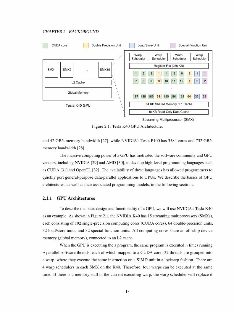
Figure 2.1: Tesla K40 GPU Architecture.
and 42 GB/s memory bandwidth [27], while NVIDIA’s Tesla P100 has 3584 cores and 732 GB/s
memory bandwidth [28].
The massive computing power of a GPU has motivated the software community and GPU
vendors, including NVIDIA [29] and AMD [30], to develop high-level programming languages such
as CUDA [31] and OpenCL [32]. The availability of these languages has allowed programmers to
quickly port general-purpose data-parallel applications to GPUs. We describe the basics of GPU
architectures, as well as their associated programming models, in the following sections.
2.1.1 GPU Architectures
To describe the basic design and functionality of a GPU, we will use NVIDIA’s Tesla K40
as an example. As shown in Figure 2.1, the NVIDIA K40 has 15 streaming multiprocessors (SMXs),
each consisting of 192 single-precision computing cores (CUDA cores), 64 double-precision units,
32 load/store units, and 32 special function units. All computing cores share an off-chip device
memory (global memory), connected to an L2 cache.
When the GPU is executing the a program, the same program is executed n times running
n parallel software threads, each of which mapped to a CUDA core. 32 threads are grouped into
a warp, where they execute the same instruction on a SIMD unit in a lockstep fashion. There are
4 warp schedulers in each SMX on the K40. Therefore, four warps can be executed at the same
time. If there is a memory stall in the current executing warp, the warp scheduler will replace it
13
CHAPTER 2. BACKGROUND
with a ready-to-execute warp in the queue. The context switching between the warps incurs very
small overhead as each thread has its own private memory space, allocated from the register file on
each SMX, to store its current state. The Tesla K40 provides 64KB on-chip memory, which can
be split between user-managed shared memory and device-managed L1 cache using one of three
configurations : 1) 48KB to 16KB, 2) 32KB to 32KB, or 3) 16KB to 48KB.
A GPU serves as a co-processor to the CPU, and often resides on its own chip, separated
from the CPU. The GPU has its own device memory (global memory) and communicates with the
CPU’s host memory through the PCIe bus. Recently there have been efforts, such as NVIDIA’s
Tegra [33] and AMD’s APU [34], that place a CPU and a GPU on the same die, sharing resources
such as memory and address space. In this thesis, we analyze the performance of Hadoop on APUs
as preliminary work. We also focus on discrete GPUs, as they provide more computing cores and
faster memory. In the following sections, we discuss the programming models that are used on GPUs
(CUDA) and heterogeneous systems (OpenCL).
2.1.2 CUDA
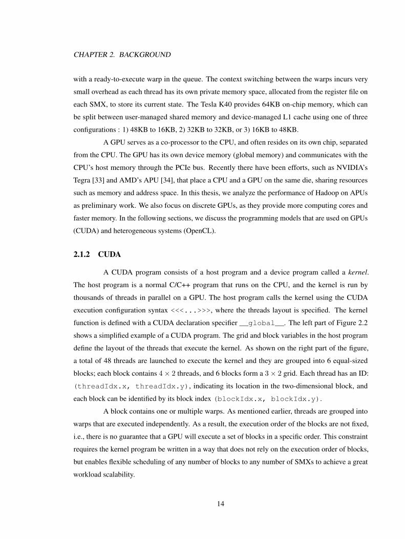
A CUDA program consists of a host program and a device program called a kernel.
The host program is a normal C/C++ program that runs on the CPU, and the kernel is run by
thousands of threads in parallel on a GPU. The host program calls the kernel using the CUDA
execution configuration syntax <<<...>>>, where the threads layout is specified. The kernel
function is defined with a CUDA declaration specifier __global__. The left part of Figure 2.2
shows a simplified example of a CUDA program. The grid and block variables in the host program
define the layout of the threads that execute the kernel. As shown on the right part of the figure,
a total of 48 threads are launched to execute the kernel and they are grouped into 6 equal-sized
blocks; each block contains 4× 2 threads, and 6 blocks form a 3× 2 grid. Each thread has an ID:
(threadIdx.x, threadIdx.y), indicating its location in the two-dimensional block, and
each block can be identified by its block index (blockIdx.x, blockIdx.y).
A block contains one or multiple warps. As mentioned earlier, threads are grouped into
warps that are executed independently. As a result, the execution order of the blocks are not fixed,
i.e., there is no guarantee that a GPU will execute a set of blocks in a specific order. This constraint
requires the kernel program be written in a way that does not rely on the execution order of blocks,
but enables flexible scheduling of any number of blocks to any number of SMXs to achieve a great
workload scalability.
14

CHAPTER 2. BACKGROUND
Figure 2.2: CUDA Execution Model and Memory Hierarchy.
15

CHAPTER 2. BACKGROUND
(a) OpenCL Execution Model [35].
(b) OpenCL Memory Model [35].
Figure 2.3: OpenCL Execution and Memory Model
CUDA has a memory hierarchy that includes various memory spaces designed with
different memory speeds and capacities. Each thread has its own private memory, allocated from
the on-chip register file; the register file has the highest bandwidth, but it is limited in size. Shared
memory is an on-chip memory that is only a bit slower than the registers; it is accessible by threads
that are in the same block, therefore can be used for intra-block communications. The global memory
is the largest memory on a GPU; its size often ranges from 2GB to 16GB. But since it is off-chip, it
is also the slowest memory: the global memory access latency can be orders of magnitude higher
than that of the shared memory. Global memory is accessible by all the threads in the grid; it can be
used for inter-block communications and it is the first storage media when the data is transferred to
the GPU. Constant memory and texture memory are both read-only off-chip memory spaces that are
shared by all threads. They can be utilized in fine-tuned CUDA programs to reduce global memory
usage to achieve better performance. Note that besides the registers, each thread also has local
memory that serves as a private storage space; when the register count is low, local memory can be
used to reduce the register pressure. However, local memory is part of the off-chip global memory,
therefore has a much longer access latency than the registers.
2.1.3 OpenCL
OpenCL is an open standard for cross-platform parallel programming developed and
maintained by the Khronos consortium [36]. The application programming interface (API) in
16

CHAPTER 2. BACKGROUND
OpenCL uses the C language wrapped by the C++ Wrapper API. OpenCL provides an abstract
hardware model for different architectures. An OpenCL program can be compiled and mapped to
different platforms such as x86 CPUs, GPUs, ARM processors, and FPGA. OpenCL defines an
execution model that describes the relationship between computation and processing units, and a
hierarchical memory model.
Similar to CUDA, OpenCL also specifies a host side (e.g., a CPU) and a device side (e.g.,
a GPU). As shown in Figure 2.3a, the device is connected to the host through a network (e.g., a GPU
is connected to a CPU via the PCIe bus). The device contains a certain number of compute units, and
each compute unit is composed of a fixed number of processing elements. A software work-item
is assigned to one processing element, and multiple work-items form a work-group. The whole
computation domain is called ND-range, which consists of multiple equal-sized work-groups. 64
work-items are grouped into a wavefront — similar to a warp in CUDA — where they are executed
in a lockstep fashion.
The OpenCL memory model has a similar hierarchical structure as CUDA. As shown
in Figure 2.3b, the device memory contains three levels: global memory (part of which is used as
constant memory), local memory, and private memory. The global memory serves the same purpose
as the one in the CUDA architecture: large, slow, and shared by all the work-items. Local memory in
OpenCL corresponds to the shared memory in CUDA: it is a fast on-chip memory space, shared by
work-items within the same work-group. Private memory corresponds to the registers in CUDA; it is
an on-chip, fast, small memory space that is only visible to an individual work-item.
2.2 Distributed Systems
The conventional approach of processing huge datasets on a distributed computing system
requires a lot of effort. Message Passing Interface (MPI) is one of the most popular standards for
distributed computing and high performance computing systems, and multiple open and vendor-
specific implementations of MPI have been developed and widely used. However, the development
process of an MPI application is complicated and error-prone. The developer needs to manually
partition the input data to be distributed, send/receive each chunk of data to/from multiple remote
machines, apply operations on different partitions of data in parallel, manage synchronization
between peers and the host machine, design a scheduler to balance the workload among machines,
and recover from failed tasks should any machine not work properly. To overcome these obstacles,
programming models such as MapReduce have evolved in recent years, simplifying data analysis tasks
17
CHAPTER 2. BACKGROUND
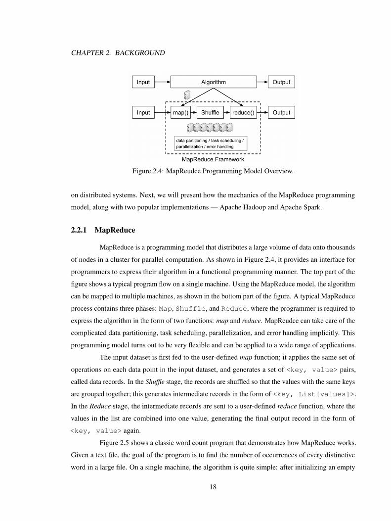
Figure 2.4: MapReudce Programming Model Overview.
on distributed systems. Next, we will present how the mechanics of the MapReduce programming
model, along with two popular implementations — Apache Hadoop and Apache Spark.
2.2.1 MapReduce
MapReduce is a programming model that distributes a large volume of data onto thousands
of nodes in a cluster for parallel computation. As shown in Figure 2.4, it provides an interface for
programmers to express their algorithm in a functional programming manner. The top part of the
figure shows a typical program flow on a single machine. Using the MapReduce model, the algorithm
can be mapped to multiple machines, as shown in the bottom part of the figure. A typical MapReduce
process contains three phases: Map, Shuffle, and Reduce, where the programmer is required to
express the algorithm in the form of two functions: map and reduce. MapReudce can take care of the
complicated data partitioning, task scheduling, parallelization, and error handling implicitly. This
programming model turns out to be very flexible and can be applied to a wide range of applications.
The input dataset is first fed to the user-defined map function; it applies the same set of
operations on each data point in the input dataset, and generates a set of <key, value> pairs,
called data records. In the Shuffle stage, the records are shuffled so that the values with the same keys
are grouped together; this generates intermediate records in the form of <key, List[values]>.
In the Reduce stage, the intermediate records are sent to a user-defined reduce function, where the
values in the list are combined into one value, generating the final output record in the form of
<key, value> again.
Figure 2.5 shows a classic word count program that demonstrates how MapReduce works.
Given a text file, the goal of the program is to find the number of occurrences of every distinctive
word in a large file. On a single machine, the algorithm is quite simple: after initializing an empty
18

CHAPTER 2. BACKGROUND
Hello WorldGood MorningWorld
Map()
<Hello,1> <World,1><Morning,1> <Reduce,1>
Node 1
Node 2
Reduce()<Hello,[1,1]><Map,[1]>
<Morning,[1,1]><Reduce,[1,1]><World,[1]>
Node 1
split & send Shuffle split & send
Reduce()
<Hello,2><Map,1>
<Morning,2><Reduce,2><World,1>
merge & send
<Hello,[1,1]><Map,[1]><Morning,[1,1]><Reduce,[1,1]><World,[1]>
Intermediate Data
Hello MapMorning Reduce
Map()
<Hello,1> <Map,1><Morning,1> <Reduce,1>
Node 2
Hello WorldGood Morning WorldHello MapMorning Reduce
Input Data
<Hello,2><Map,1><Morning,2><Reduce,2><World,1>
Output Data
Figure 2.5: Counting Occurrences of Words in a Large Text File using MapReduce.
hashmap, we read in the text file word by word and insert the word as the key, and 1 as the
value into the hashmap, if the word does not exist in the hashmap; otherwise, we use the given
word as the key to search the hashmap, and increase the corresponding value by 1. But when the
file becomes too big to fit in the memory on a single machine, or the execution time is too long,
we need to use multiple machines to count the words in parallel for a shorter turnaround time.
Processing this file in a distributed system is not trivial: it requires partitioning the data with balanced
workloads on each machine, combining hashmaps from each machine, and recovering data when
machines fail, etc. MapReduce automatically deals with the aforementioned issues, as long as the
programmers cast their algorithm into map() and reduce() functions. Figure 2.5 shows how we can
process this file in a distributed manner using the MapReduce model. The map function outputs
<word, 1> for every word parsed from the text file (e.g., <Hello, 1> and <World 1>). Note
that this function runs on two machines simultaneously where each machine only processes half
of the input dataset. These key-value records are shuffled by the framework and converted into
<word, List[1, 1, 1, ...]> (e.g., <Hello, [1, 1]>), where each record contains a
unique word, followed by a list of all the 1s generated in the previous stage. The shuffle stage is
carried out on a central machine. The shuffled records are then sent to two machines where the
reduce() sum up the partial counts locally. The partial counts are then merged to generate the final
19
CHAPTER 2. BACKGROUND
JobTrackerMapReduce Program
NameNodeClient
Assign/return tasks Assign/return tasks
HDFS
DataNode
child JVM
map()reduce()
TaskTracker
Launch
DataNode
child JVM
map()reduce()
TaskTracker
Launch
read/write
read/write read/write
Figure 2.6: Hadoop Framework.
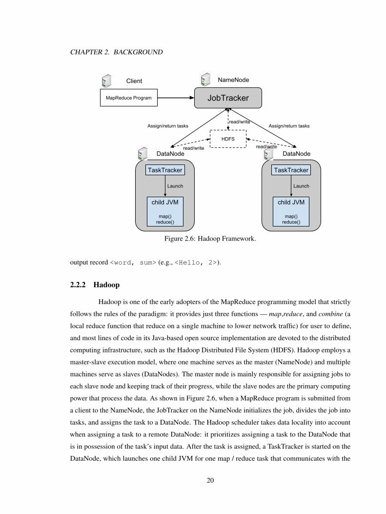
output record <word, sum> (e.g., <Hello, 2>).
2.2.2 Hadoop
Hadoop is one of the early adopters of the MapReduce programming model that strictly
follows the rules of the paradigm: it provides just three functions — map,reduce, and combine (a
local reduce function that reduce on a single machine to lower network traffic) for user to define,
and most lines of code in its Java-based open source implementation are devoted to the distributed
computing infrastructure, such as the Hadoop Distributed File System (HDFS). Hadoop employs a
master-slave execution model, where one machine serves as the master (NameNode) and multiple
machines serve as slaves (DataNodes). The master node is mainly responsible for assigning jobs to
each slave node and keeping track of their progress, while the slave nodes are the primary computing
power that process the data. As shown in Figure 2.6, when a MapReduce program is submitted from
a client to the NameNode, the JobTracker on the NameNode initializes the job, divides the job into
tasks, and assigns the task to a DataNode. The Hadoop scheduler takes data locality into account
when assigning a task to a remote DataNode: it prioritizes assigning a task to the DataNode that
is in possession of the task’s input data. After the task is assigned, a TaskTracker is started on the
DataNode, which launches one child JVM for one map / reduce task that communicates with the
20

CHAPTER 2. BACKGROUND
Figure 2.7: Spark Framework.
HDFS. The JobTracker maintains a heartbeat communication with the TaskTrackers, if a TaskTracker
is lost caused by a node failure, the JobTracker can resubmit the task to another available DataNode.
When a task is completed, the child JVM is released after it writes the output to the HDFS, and
the JobTracker is noticed that the TaskTracker is available for a new task. Because HDFS is based
on disks, frequent read and write accesses in MapReduce jobs incur a large I/O overhead. In the
next section, we describe Spark, an in-memory processing engine for distributed workloads that
significantly reduces such I/O overhead.
2.2.3 Spark
Spark has a similar master-slave execution model as Hadoop. As shown in Figure 2.7,
the master node is called driver node while the slave nodes are called worker nodes. Spark’s main
program is called driver program that sits on the driver node. The SparkContext object contained
in the program consists of the information to coordinate the data and job distributions. When a
Spark job is launched, the SparkContext connects to a specific cluster manager, such as Mesos
or YARN, to carry out the following operations: 1) it allocates resources on each worker node, 2) it
starts an executor on each work node, which spawns multiple processes to wait for incoming tasks,
3) it sends the user program to the executors, and 4) it sends tasks to the executors to run. Note that
Spark can still read and write data from a distributed file system such as HDFS, but the executor can
21

CHAPTER 2. BACKGROUND
be instructed to cache data in the memory for the duration of the whole application to significantly
reduce the amount of I/O operations.
The core of Spark is built on its Resilient Distributed Datasets (RDDs). An RDD is used
to wrap an array of elements, and divide them into multiple partitions which can be distributed to
multiple worker nodes for parallel processing. An RDD is created by applying a transformation
operation on data either from the stable storage (i.e. from the disk), or another RDD. For example,
a map transformation takes in a user-defined function and applies that function to every element
in the RDD. Transformations are lazily executed — i.e., Spark does not execute the map function
right away to generate the child RDD — it only saves the information of how this child RDD can
be transformed from its parent RDD. This information is used to build a lineage graph that tracks
a chain of transformations to be applied to the ancestor RDD in order to generate the result RDD.
This lineage graph is crucial when it comes to recovering data in case of a node failure; the missing
RDD can be reconstructed by re-computing each stage in its lineage graph, starting from the very
first ancestor RDD in the stable storage. The data recovery eliminates the expensive overhead of
disk-based data checkpointing used in Hadoop. A typical driver program starts by defining one or
multiple RDDs and calls transformations that are performed on them. To produce the final result
of a transformed RDD, users need to apply an action operation, such as reduce (which combines
multiple data points into one), count (which returns the number of data points in an RDD) or collect
(which executes all the transformation operations and returns the whole result RDD to the driver
node). In addition, the persist method can be called with an RDD to indicate that the data will be
reused later in the program. Spark caches as many persistent RDDs in memory as possible, and spills
them to disk if it runs out of space. This caching mechanism greatly improves performance when the
same RDD is repeatedly accessed, e.g., when an RDD is used to store the data points that update the
gradient value iteratively in the logistic regression example shown in Listing 1.1.
Figure 2.8 shows the the lineage graph of the logistic regression example, constructed
by Spark during runtime. Each RDD data is given a unique ID. By calling cache() on the RDD
points, Spark persists the RDD in memory. As a result, points of RDD1 are reused in the second
iteration, while a new RDD RDD3 is created for the gradients. Instead of repeatedly parsing the
data from the storage data in each iteration (as indicated by the dashed line), we can directly read
points from memory. This significantly improves performance for ML algorithms, where a model
is iteratively trained from the same input dataset.
Another important use of a lineage graph is for data recovery when there is a node failure;
the missing RDDs can be reconstructed by re-computing each stage in the lineage graph. The
22

CHAPTER 2. BACKGROUND
Figure 2.8: Lineage graph for logistic regression, different data structures are represented with
different shapes
re-computation is entirely done in memory, avoiding expensive disk-based data checkpointing used
in Hadoop.
23
Chapter 3
Related Work
In this chapter, we first review related work that focuses on leveraging GPUs in MapReduce-
based distributed systems. Then we describe our preliminary work, which utilizes heterogeneous
systems under the Hadoop framework to accelerate a recommender system.
3.1 MapReduce-based Distributed Systems with GPUs
There have been a number of efforts that utilize GPUs leveraging the MapReduce pro-
gramming paradigm. In this section, we describe them in detail and compare them based on three
aspects:
1. Compatibility
Compatibility is an important measurement, as it characterizes how well a given framework can
be adopted by the research and software development community. For example, a Spark-based
system can inherit Spark’s critically acclaimed fault-tolerant features, efficient inter-node
communication mechanisms, and attract adoption from a large user base. In addition, if the
framework does not require changes of code in the core of Spark, but is rather a plug-and-play
3rd party library that runs directly on top of Spark, it can gain an even broader acceptance in
the community. Using a library avoids tedious code maintenance work needed in order to keep
up with the actively developed open-source project of Spark. We divide the compatibility of
related work into three categories: 1) compatible with Hadoop, 2) compatible with Spark, or 3)
stand-alone frameworks that do not depend on any existing platform.
2. Flexibility
24

CHAPTER 3. RELATED WORK
High flexibility means that the framework can be used for deploying a wide range of applica-
tions. It depends on several factors, including: 1) if the APIs provided by the framework are
easy to use, and able to express a range of algorithms efficiently, and 2) if the framework can
accommodate various data structures, such as primitive data types, user-defined classes, sparse
vectors, etc.
3. Transparency
Transparency characterizes how much a given framework exposes the GPU programming
details, and resources management tunning knobs to the programmer. To one extreme, there
are frameworks that grant the user with full access to the GPU programming model for tuning
memory allocation, grid/block configuration, task to thread mapping, etc.. Such frameworks
aim at achieving high performance using GPUs with a single programming abstraction; while
on the other end of the spectrum, the frameworks make GPUs totally transparent, striving to
enable programmers to harvest GPUs without having any knowledge about the underlying
CUDA or SIMD architectures. These two different system paradigms present a trade off
between programmability and performance.
Compatibility Flexibility Transparency
Catanzaro et al.StandaloneSingle GPU
Limited numberof map keys
Limited support forreduce operations
Users write Map in CUDAReduce is hardcoded
MarsStandaloneSingle GPU
Extra counting phases No GPU programming
MapCGStandaloneSingle GPU
Additional set of APIsNo GPU programming
Write code once, executeon both devices
GPMRStandaloneGPU cluster
Restructured MapReducepipeline
Full GPU expositionkernel tuning
thread/block configuration
HadoopCLCompatible with Hadoop
Change to Hadoop core codeStatic-typed APIs
Highly TransparentNo GPU programming
SWATCompatible with Spark
No change to Spark codePlug and play
Wrapper APIs to RDDsHighly Transparent
No GPU programming
Table 3.1: A comparison of existing frameworks.
Table 3.1 presents a comparison between related work on these three aspects. In the
25
CHAPTER 3. RELATED WORK
following sections, we will first discuss the stand-alone frameworks, and then the frameworks that
are built upon Hadoop/Spark.
3.1.1 Stand-alone Frameworks
Earlier work focuses on using MapReduce purely as a programming abstraction to alle-
viate GPU programming complexity for the average user. Adopting this model, applications are
implemented in C/C++ and CUDA/OpenCL as individual stand-alone library packages, instead of
built upon Hadoop or Spark.
To our knowledge, Catanzaro et al. [37] is the first work to adopt this model. The framework
asks the programmer to provide: 1) a map function, 2) a set of reduce operators, and 3) a cleanup
function that operates on the reduction results. The map function is arbitrary CUDA code that
produces a set of (key, value) outputs and a set of predicates for each thread. These predicates
consist of one integer per thread, which controls how reduce operations are applied to the map
outputs. The runtime then restructures the code and produces two functions. The first function
combines the user-defined map function with a local reduction operation using the reduce operators.
The second function is a global reduction, combined with the user-defined cleanup function. The
goal of the framework is not to hide GPU programming from the programmers completely, but to
help achieve good performance with less programming effort. Users still need to write map functions
in CUDA, and provide additional information such as predication and reduction operators. But they
do not need to take care of the inter-thread communication and synchronization, which are needed in
a typical CUDA program. The framework also automatically generates optimized parallel reduction
code for the user. However, the framework assumes that: 1) one map function only generates one
output, 2) the reduction operators can only be binary, 3) there are only up to 32 keys generated by the
map function, and 4) reduction functions must be associative. These assumptions limit the range
of applications that can be applied on the framework. They use Support Vector Machine (SVM) as
the benchmark to test the framework’s performance, achieving a 5x-32x speedup in training and a
120x-150x speedup in classification, compared to LibSVM [38], a popular SVM software package
running on a CPU.
Mars [39] provides for higher transparency than Catanzaro et al.’s work. It does not require
users to have any GPU programming knowledge; instead, users just need to write the MAP() and
REDUCE() function using the provided C/C++ APIs. Because the output size of the map and reduce
functions is only known during the runtime, and GPU does not support dynamic memory allocation,
26
CHAPTER 3. RELATED WORK
Mars requires the user to write two additional functions: MAP_COUNT() and REDUCE_COUNT(),
which generate the number of elements of the intermediate data, the size of the intermediate data,
and the size of the reduce results. Mars then uses this information at runtime to allocate GPU buffers
and generate a prefix sum array to indicate the write location for each thread. Mars distributes one
chunk of data to one map/reduce task, and assigns one task to one GPU thread, so that multiple
tasks can execute in parallel. The sorting of intermediate data and the final global reduction is also
done automatically on the GPU. It provides access to configuration parameters such as whether to
execute a sort or reduce stage, the number of thread blocks, and the number of threads per block,
enabling users to tune their application. But users can choose to sit back and let Mars run without any
intervention, as all these parameters have default values. Mars employs several GPU optimization
techniques, including ensuring coalesced memory accesses, utilizing built-in vector types such as
char4 and int4, and using hashing to store sorted intermediate data. They evaluate the framework
with 6 common web applications, and compare the performance results against Phoenix [40] — a
CPU-based MapReduce framework that focuses on utilizing multi-core parallelism, and achieves
1.5x - 16x speedups.
One inefficiency of Mars is that it needs to execute two additional count phases to get
around the problem of limited memory allocation support on GPUs at the time. In a worst case
scenario, the same set of operations will carried out in both the counting function and the map/reduce
function, which doubles the overall execution time.
MapCG [41] strives to be a framework that supports source code portability between
the CPU and the GPU. Users need to only write one version of their code, and the runtime can
execute the code on a multi-core CPU using OpenMP, on a GPU using CUDA, or on both platforms
simultaneously. In addition to the map and reduce functions, MapCG requires users to define three
more functions: Splitter(), Hash(), and KeyCompare(). The Splitter() defines how
to divide the workload between the CPU and GPU, while the latter two functions are mainly used
to determine how to insert data into MapCG’s internal hashtable. MapCG makes use of the newly
added atomic operation support on GPUs (which was not available to Mars at the time their work) to
implement a light-weight dynamic memory allocator for GPUs. It initially uses cudaMalloc()
to allocate a rather large memory buffer on the global memory, from which, it assigns equal sized
“buffer blocks” to the warps on the GPU. Each warp gets one buffer block, which serves as its own
private memory space. Each warp maintains a free_space_ptr that keeps track of the starting
address of the free space within the buffer block. A thread can then dynamically allocate memory
by incrementing the pointer by the requested size using the atomic operation atomicAdd(), to
27

CHAPTER 3. RELATED WORK
ensure the correctness of concurrent operations. The dynamic memory allocator gets rid of the need
of the expensive counting phases used in Mars, and together with the use of a hashtable to store the
intermediate data instead of sorting them, MapCG improves performance compared to Mars. They
evaluate the framework with 8 popular benchmarks and obtain average speedups of 1.6x-2.5x as
compared to Mars.
The aforementioned frameworks all leverage just one GPU on one compute node, and
only support in-core algorithms where the size of input data does not exceed that of a GPU’s
memory. GPMR [42] was developed to address these issues: it is a framework that streams data to a
cluster of GPU-equipped computing nodes. GPMR provides two optimization techniques: partial
reduction and accumulation, for restructuring a standard MapReduce pipeline. These techniques
aim at packing computation on a GPU as much as possible, overlapping GPU-CPU communication
with GPU computation, and reducing PCIe/network traffic. GPMR grants programmers with a very
high degree of freedom to interact with the framework’s pipeline and the GPUs, including tuning
GPU kernels, experimenting with different MapReduce pipeline configurations, and alternating
task-to-thread mapping schemes, to achieve the best performance possible. They implement five
popular benchmarks on the framework, and provide a detailed analysis on the differences between a
standard CPU-based MapReduce implementation and their optimized GPMR implementation for
each benchmark. These benchmarks range from compute-bound to memory-bound, and possess
different algorithmic scaling characteristics. They first compare the performance of GPMR versus
Mars on a single machine, where they achieve 2.7x-37x speedups using three benchmarks. Then a
full evaluation of all five benchmarks is conducted, where they analyze the weak/strong scaling of
the framework, using different sized datasets, running on 1, 4, 8, 16, 32 and 64 GPUs.
3.1.2 Hadoop/Spark Compatible Frameworks
The stand-alone frameworks provide a great foundation for exploring the potential impact
GPUs could bring to the MapReduce programming abstraction, but they all lack one critical feature
of a robust distributed system: reliability. As data sizes continue to grown unbounded, distributed
systems are scaling out to more and more compute nodes, dramatically increasing the chance of
machine failures. This is one of the major reasons why Hadoop/Spark is so popular; it supports a
robust distributed file system to store datasets that exceed a single machine’s capacity, and it uses
check-pointing/data re-computing techniques to recover from a failed node and resumes execution.
There are two GPU-enabled distributed systems that extend Hadoop/Spark: HadoopCL and SWAT,
28

CHAPTER 3. RELATED WORK
which are discussed next.
HadoopCL [43] integrates OpenCL devices into Hadoop to accelerate classic Hadoop
workloads. It hides GPU programming complexity by using Aparapi [44] to automatically translate
a user-written Java program’s bytecode to an OpenCL program. The OpenCL code then runs
on both CPUs and GPUs in a heterogeneous computing environment, managed by HadoopCL’s
runtime system. HadoopCL directly extends Hadoop’s Mapper and Reducer classes to increase code
portability — programmers need to make only small changes to their existing Hadoop program in
order to make their program compatible with HadoopCL. HadoopCL’s runtime maintains multiple
threads that support asynchronous kernel launches and data transfer, to increase the utilization of the
network and device bandwidths, while keeping the GPU occupied. The authors evaluate HadoopCL
by running four benchmarks. While the throughput of just the map task is fairly high, ranging from
1.69x-55.41x as compared to their Hadoop counterparts, the end-to-end execution only achieves
a 1.07x-2.07x speedup for the same set of benchmarks. This leads to their conclusion that, while
heterogeneous processors could provide a significant performance benefit, the bottleneck in Hadoop
is often the I/O overhead (i.e., read/write operations in the HDFS), which obscures any throughput
gains from using accelerators. Other limitations of HadoopCL include: 1) it only supports Java
variables of primitive types, restricting the flexibility of adapting to a wider range of applications, and
2) it does not allocate GPU memory dynamically, needing programmers to define a helper function
so that the runtime can pre-allocate GPU memory.
HadoopCL2 [45] is built from scratch based on the insights gained through developing
HadoopCL. It features an auto-scheduler, which dynamically assigns a task to one of three devices
— the original Hadoop JVM, an OpenCL CPU device, or an OpenCL GPU device — based on the
current system load on different devices and the task’s historical performance information. This
could significantly increase the system’s performance as some applications run much faster within a
JVM versus on a GPU. HadoopCL2 also supports additional data types, including sparse vectors and
composites, which increases its applicability to a wider range of ML algorithms. In addition, it adds a
dynamic memory allocator (similar to MapCG’s) for GPUs, and a GPU-based garbage collector that
enables a thread to reclaim temporary memory allocations. These improvements produce 1.04x-1.60x
additional speedup, for the benchmarks tested versus the original HadoopCL. They also tested 5
complex ML applications from Mahout [46] and achieved a 1.09x-21.32x speedup, while finding
similar strong scaling as compared to Hadoop run on 2-8 computing nodes. The performance gains
are obtained by using manual scheduling — an optimal selection of devices for each task based
on extensive testing of a variety of configurations. They also evaluate the auto-scheduler against
29
CHAPTER 3. RELATED WORK
the manual configuration; it can match or beat the manual scheduler, resulting in a 0.83x-1.06x
speedup. We use HadoopCL2 in our preliminary work in Section 3.2, where we refer to HadoopCL2
as HadoopCL for simplicity.
As Spark employs low latency memory as its storage for intermediate data, we observe a
shift in where the bottlenecks in a distributed system occur, moving from the disk I/O subsystem,
to CPU throughput and memory bandwidth. This shift makes the GPU’s computing power more
prominent in determining the overall system performance, since the benefits of high throughput
processing are no longer hidden by the I/O overhead. SWAT [47] integrates GPUs in Spark to harvest
such benefits. Developed by the same group that developed HadoopCL, SWAT continues the use
of APARAPI for automatic OpenCL code generation in order to make GPU programming details
transparent to programmers; it only requires the programmer to wrap a Spark RDD with a custom
SWAT RDD object, using a “cl” API call. They extend APARAPI to support SparseVector and
DenseVector in Spark MLlib [48], adding a Spark-based machine learning library, as well as the
Tuple2 class in Scala (used to store key-value pairs in Spark). The SWAT runtime is asynchronous,
event-driven, and resource-aware; it is built on top of Spark without any modifications to Spark’s
core code. SWAT supports caching broadcast variables, but does not support caching RDD partitions
in GPU memory, and it does not utilize the GPU’s constant or shared memory. They evaluate
the framework by rewriting and executing six machine learning applications on SWAT, using 2,
4, and 8 computing nodes, each of which consists of a 12-core CPU and two NVIDIA M2050
GPUs. For compute-bound applications, SWAT achieves up to a 3.25x speedup, while for I/O-bound
applications, SWAT produces similar or slightly worse performance, as compared with Spark. In
addition, SWAT presents similar strong scaling characteristics, as does Spark. The authors also
consider using finer granularity during profiling to study the reasons behind the performance results;
they look at task-level speedups, break down the overall runtime into input, execution, and output
time, and study OpenCL event profiling results.
3.2 Preliminary Work
In this section, we discuss our preliminary work which accelerates a Mahout recommender
system by deploying it on GPU-enabled clusters using HadoopCL. Observing some performance is-
sues posed by HadoopCL’s highly automatic memory management system, we propose a cooperative
HadoopCL model that achieves better performance by exposing more GPU programming details to
the programmer.
30

CHAPTER 3. RELATED WORK
userIDitemID
0 1 2 3 4 5
1001
1002
1003
1004
0.0 0.0 0.0 0.03.0
0.0 4.0 0.0 0.0 3.54.5
5.0
0.0 0.0 0.0 3.03.5
0.0 0.0 0.0 4.0 2.0
5.0
4.5
0 1 2 3 4 5
0 0 0 00 00
1
2
3
4
5
0 0 0 0.780 0.39
0 0 00 0
0 0 0.530 0.91
0.78 0 00.53 0.75
0.39 0 0.750.91 0
0.0
0.0
0.0
3.0
0.0
5.0
1001itemID
itemID
=
0.0
1.95
0.0
4.55
5.34
2.73
recom
User Matrix
Similarity Matrix Recommendation Vector for user 1001
0
0
0
0
X
Figure 3.1: An example of Mahout processing a movie ratings dataset.
3.2.1 Mahout
Mahout [49] is an open source machine learning library built upon Hadoop, enabling
parallel processing of big data on a distributed system. Mahout implements three machine learning
techniques: 1) recommendation engines, 2) clustering, and 3) classification. We focus on the
recommendation engine in this preliminary work. A recommender system makes personalized
recommendations for merchandise such as movies, apparel, and electronic devices to customers based
on their purchasing history. It is being widely used on e-commerce websites such as Amazon [50]
and Netflix [51]. The Mahout recommender is based on collaborative filtering (CF). There are two
common methods used in collaborative filtering — neighborhood-based methods [52, 50, 53], and
latent factor models [54].
Using a neighborhood-based method, the system explores the relationship between users
(user-based collaborative filtering) and items (item-based collaborative filtering). To recommend an
item to user u, the system can either find users that are similar to u, and recommend to u the items
that were positively endorsed by those users, or the system can find the items that are similar to those
that user u has rated positively, and recommend those items to u.
An alternative approach is to use a latent factor model. Instead of characterizing the
relationship between users, or alternatively, between items, the model describes both users and
items in a latent factor domain. Unlike the human-created genres, the latent factors comprise a
computerized alternative that can uncover complicated relationships that are not manually defined,
such as a group of movies with product placements, or two products with totally different user bases.
Mahout uses item-based CF in its recommendation system. Figure 3.1 shows how Mahout
31

CHAPTER 3. RELATED WORK
3 4 5
3
4
5
0.530.76 0.64
0.390 0.46
00 0.55
itemID
itemID
Similarity Matrix
userIDitemID
3 4 5
Normalized User Matrix
map() reduce()intermediatedata
Shuffle intermediatedata
3 4 5
0.33 0.30 0.323
4
5
0 0.27 0.29
0 0.300
itemID
itemID
3 4 5
0.333
4
5
0
00
itemID
itemID
1003
1004
0.520.57
0.65 0.35
0.55
0.49
0.33 0.30 0.323
0.43 0.23 0.32
3 4 5
3
4 5
4 0.27 0.29
4 0.12 0.17
3
0
0
4 5
5 0 0.30
3
0
3 4 5
0.43 0.23 0.323
4
5
0 0.12 0.17
0 0.250
itemID
itemID
3
5 0 0.250
Figure 3.2: The PairwiseSimilarity job in Hadoop.
processes a movie ratings dataset. The input data is an n× d matrix, where each row represents a
user, each column represents an movie, and each entry (i, j) represents user i’s rating for movie j.
Mahout then generates a d× d similarity matrix from the user matrix, whose entry (i, j) represents
the similarity between item i and item j. To generate the recommendations for a user, Mahout
multiplies the similarity matrix with the target user’s rating vector. The result is a d-dimensional
recommendation vector where entry i represents the recommendation score for item i. User 1001’s
recommendation vector in Figure 3.1 shows that item 4 is to be recommended as it has the highest
score of 5.34. The whole recommender system consists of 8 Hadoop jobs. We profile Mahout
on 2, 4, and 8 computing nodes and we observe that those 8 Hadoop jobs are bottlenecked by the
pairwiseSimilarity job, which corresponds to the stage in which the similarity matrix is
generated. In the following sections, we describe pairwiseSimilarity job in Mahout, and our
implementations using HadoopCL and cooperative HadoopCL.
3.2.2 PairwiseSimilarity Job in Mahout
Because MapReduce processes data in the unit of (key, value) records, the rows of
the user matrix are represented by records and distributed to multiple machines. Figure 3.2 shows
32

CHAPTER 3. RELATED WORK
userIDitemID
0 1 2 3 4 5
1001
1002
1003
1004
0.0 0.0 0.0 0.00.49
0.0 1.0 0.0 0.0 0.380.78
0.55
0.0 0.0 0.0 0.520.57
0.0 0.0 0.0 0.65 0.35
0.55
0.49
Normalized User Matrix
1001
Key(int) value(HashMap)
[3:0.49 5:0.55]
1002 [1:1.0 4:0.78 5:0.38]
1003 [3:0.57 4:0.52 5:0.55]
1004 [3:0.65 4:0.35 5:0.49]
Mahout Format
3 5 1 4 5 3 4 5 3 4 5
0.49 0.55 1.0 0.78 0.38 0.57 0.52 0.55 0.65 0.35 0.49
0 2 5 8
0 2 5 8
1001 1002 1003 1004
indexLookUpTable
valueLookUpTable
keyArray
indexArray
valueArray
HadoopCL Format
Figure 3.3: Data Format in Mahout and HadoopCL.
how the rows of a user matrix of two users 1003 and 1004 are distributed to two machines for the
item similarity computation. In the map phase, Hadoop iterates over every user vector and generates
a partial similarity matrix for each user. The partial similarity matrix contains similarity scores
between items which were rated by that user. For example, a partial similarity matrix of items 3-5 is
generated for user 1003, who has rated these three and only these three items. In the shuffle phase,
the partial similarity matrices generated by different users are then sorted so that the data from the
same row of the partial similarity matrix are placed into a consecutive chunk. During the reduce
phase, each chunk is processed by the reduce function where the similarity scores are summed up to
generate the final similarity matrix.
Since the matrices used in a recommender system are usually very sparse, Mahout only
stores non-zero values on the HDFS. The key in a (key, value) record is used to store the row
index, while the value is a HashMap that stores the column index and the value of the matrix entry.
The middle part of Figure 3.3 shows how the user matrix is stored in Mahout.
3.2.3 PairwiseSimilarity Job in HadoopCL
HadoopCL uses GPUs only for the map phase since it is the performance bottleneck of the
job. There is minimum code change in Mahout to enable the execution on GPUs with automatically
generated OpenCL code; but under the hood, there is major data transformation to better utilize
the GPUs. Instead of using a HashMap, which lowers GPU’s throughput by frequent atomic and
search operations [55], HadoopCL uses linear arrays along with look-up tables to store the sparse
matrices. As shown in the right hand side of Figure 3.3, the keyArray stores the keys that represent
the userIDs, and the indexArray and valueArray store the itemIDs and the rating values
33

CHAPTER 3. RELATED WORK
respectively. Searching an entry through these arrays is enabled by using two associated look-up
tables constructed by using prefix-sum algorithm [56].
50.57
keyArray indexArray valueArray work-item work-group
1003 1004
3 4 5 3 4
0.550.52 0.65 0.35
3
4
3
4
5
0.57
0.52
0.65
0.35
0.490.55
1003 1004
Input/Output chunk
Original HadoopCL
transpose5
0.49
0.33
3 4 5
0.320.30
3 4 5
4 5 5
0.27 0.300.29 0.13
3 4 5
0.320.23
3 4 5
4 5 5
0.12 0.250.17
0.57
3 4 5
3 4
0.550.52
0.65 0.35
1003
1004
5
0.49
0.33
3 4 5
0.320.30
3 4 5
4 5 5
0.27 0.300.29
0.13
3 4 5
0.320.23
3 4 5
4 5 5
0.12 0.250.17
Cooperative HadoopCL
Figure 3.4: HadoopCL vs. cooperative HadoopCL.
The left hand side of Figure 3.4 shows how HadoopCL process the Mahout job shown
in Figure 3.2 with transformed data. Instead of iterating through every user vector sequentially,
HadoopCL processes each user vector (consists of three arrays) in parallel, where each user vector is
assigned to a work-item, which generates its own partial similarity matrix.
We conduct a preliminary experiment to evaluate HadoopCL’s performance on the pair-
wiseSimilarity job. We first run the whole job on HadoopCL using a CPU v.s. a GPU. For these
experiments we use two systems: one with an AMD A10 APU in each node, and one with an
NVIDIA K20M in each node. System configurations are shown in Table 3.2.
Table 3.2: Hardware configurations used in this study.APU NVIDIA
NameNode DataNode NameNode & DataNodeCPU AMD A8-3850 AMD A10-6700 Intel Xeon E5-2650GPU AMD Radeon HD 6550D AMD Radeon HD 8670D NVIDIA Tesla K20m
CPU Cores 4 4 32GPU Cores 5 6 13CPU Freq 2.9GHz 3.7GHz 2GHzGPU Freq 600MHz 844MHz 706MHz
Our results show that in HadoopCL, the job takes twice as long to run on the GPU versus
the CPU. To investigate the factors that slow down the GPU execution, we extract the CPU and GPU
OpenCL code generated by Aparapi in HadoopCL and compare the performance of the stand-alone
kernel running on CPU and GPU.
34
CHAPTER 3. RELATED WORK
A10 APU K20m10
0
101
102
103
104
Executi
on T
ime (
ms),
Log S
cale 5402.19
1636.89
38.09 40.7827.45
10.98
GPU
CPU
OPT
(a) The HadoopCL kernel performance comparison.
sorting loop writing validation0
500
1000
1500
2000
2500
3000
Execution Time (m
s)
575/11%
2850/52%
1632/30%
361/7%
(b) The HadoopCL GPU execution breakdown.
Figure 3.5a shows that, on both systems, the GPU execution time is much longer (up to
142x) than that of the CPU. Note that the y-axis is in log scale so that the GPU execution time can fit
in the figure. The next section will analyze reasons for this GPU performance loss and discuss our
HadoopCL cooperative model.
3.2.4 HadoopCL Cooperative Model
Figure 3.5b shows a breakdown of the execution time of the GPU code generated by
Aparapi in HadoopCL. The execution is divided logically into four parts. The first part is spent
sorting, where every work-item sorts a small chunk of the indexArray and the valueArray. Because
sorting exhibits random memory behavior (which can become a performance barrier for the GPU),
we add a Filter phase on the CPU before the map phase on the GPU so that the performance impact
of sorting is diminished.
The main part of the GPU code is a two-level nested loop where the partial similarity
scores are generated. HadoopCL uses a work-item to process a whole user vector. For a user vector
of n elements, HadoopCL generates an indexArray and a valueArray whose lengths are bothn×(n+1)
2 , as well as a keyArray of length n. Since n denotes the number of ratings given by a
user, the workload for each work-item can differ greatly. If we denote nmax and nmin as the largest
and smallest number of movies rated by a user, the work-item processing nmin ratings is stalled for
Θ(nmax2−nmin
2) cycles to wait on the completion of the busiest work-item in the same work-group.
This can leave a large number of work-items idle.
The pairwiseSimilarity job serves as a good example of the performance issues that can
arise when mapping one map/reduce task to one work-item. This simple model does not work well
for applications which can benefit from intra work-group communications. To solve this issue, we
propose a cooperative HadoopCL model which provides more flexibility for programmers to deal
with such problems, and can offer many applications improved performance. This model allows
35
CHAPTER 3. RELATED WORK
customized OpenCL kernels to be integrated into HadoopCL to execute specific applications more
efficiently. By allowing programmers to still write their applications in Java, auto-generate OpenCL
kernels, and then manually tweak the generated OpenCL kernels for performance, the cooperative
model still maintains a high degree of programmability while offering improved performance for
applications that can benefit from lower-level tuning. The right hand side of Figure 3.4 shows how
the cooperative model processes the user vectors in the pairwiseSimilarity job. Instead of assigning
an entire user vector to one work-item, the new kernel cooperatively processes each user vector
with a work-group. In this model, the number of stalls is reduced from Θ(nmax2 − nmin
2) to
Θ(nmax − nmin).
The remaining two parts of the GPU implementation are writing and validation. HadoopCL
supports dynamic memory allocation in OpenCL, since it assumes the size of the output and the
writing location of each work-item is unknown. However, dynamic memory allocation adds overhead
and so is measured in the writing stage. The validation part notifies the host to restart processing
if dynamic memory allocation fails. In the cooperative model, we are able to determine the output
size, as well as the output location for each work-item. Therefore, the expensive atomic operations
used during dynamic memory allocation are eliminated. And as a side effect, validation is no longer
necessary needed.
We evaluate the cooperative model by executing the original kernel on CPU/GPU, and the
optimized kernel on GPU on both platforms. As shown in Figure 3.5a, the optimized GPU kernel
(OPT) achieves a speedup of 1.38X and 196X when compared with the original CPU/GPU kernel on
the APU platform, and 3.8X and 149X on the K20M platform.
3.2.5 Conclusion
HadoopCL offers great programmability and a Hadoop-like interface to allow users to pro-
cess their data using GPUs transparently. However, the trade-off is that the user loses the opportunity
to write fine-tuned GPU programs to really leverage its performance. This limitation sometimes
even leads to significant performance degradation compared to a CPU-based implementation. This
observation motivates us to develop a framework that allows the integration of manually written
GPU kernels, while maintaining a high-level programming interface and keeping other aspects of
distributed computing transparent to the users.
36
Chapter 4
Enabling Accelerators on Spark System
In this chapter, we describe the framework design by describing 1) the functionality of
GPUEnabler, 2) the extensions we developed on top of GPUEnabler to enable an efficient and flexible
runtime, and 3) the performance evaluation of the extended GPUEnabler.
4.1 GPUEnabler
To enable Spark to seamlessly leverage a GPU, we need to create an efficient mapping
mechanism from a partition of data in RDDs, to the thread blocks on a GPU. There are three
challenges to address when performing this mapping: 1) GPUs need to process a large chunk of
consecutive data items on each kernel invocation, using a large number of threads in order to hide
memory latency and to amortize the cost of context creation and kernel launch. This is not compatible
with Spark’s iterator-based executor model; 2) because RDDs sit on the JVM’s heap memory, for
a GPU to access it, we need to transfer the data from on-heap memory to off-heap memory, and
then transfer it to GPU memory. Additional considerations need to be taken into account in order to
minimize the transfer frequency between these different memory spaces.
To address these issues, GPUEnabler provides a versatile class named HybridIterator
to convert a partition of an RDD to a chunk of consecutive memory stored off the heap. Figure 4.1
uses logistic regression algorithm as an example to illustrate how the HybridIterator manages different
types of memory buffers. The input is a set of data points and the corresponding labels, which
represent the classes the data points belong to. A data point is represented as a d-dimensional array,
and the class label is stored as an integer. In Spark, the input can be represented by an RDD of a
case class RDD[DataPointAndLabel], where the case class DataPointAndLabel consists
37

CHAPTER 4. ENABLING ACCELERATORS ON SPARK SYSTEM
Figure 4.1: An overview of GPUEnabler.
of an array and an integer as its member variables. Spark stores a set of DataPointAndLabels
in an iterator. HybridIterator transforms the iterator of n objects into two buffers. The first
buffer stores an array of n× d elements, generated by concatenating n d-dimensional data points
together; the second buffer stores and array of n integers, which are the labels extracted from the
DataPointAndLabel objects in the iterator. Each buffer is placed into a chunk of consecutive off-
heap memory, and then transferred to the GPU’s device memory before a kernel is launched. During
this process, CUDA streams are used to overlap data transfers and kernel executions. GPUEnabler
uses JCUDA [57] — a Java to CUDA library backed by the Java Native Interface [58] — to manage
these operations.
Transferring data from Spark’s RDD to consecutive memory off the heap, and then to the
GPU’s memory, is quite expensive. To save the transfer overhead for reused data, users can call
rdd.cacheGPU() on a GPU-backed RDD to persist the data on the GPU. This is analogous to
Spark’s rdd.cache() call, which preserve the data on the system memory.
Another major component of GPUEnabler is a class called CUDAFunction, as shown
on the right hand side of Figure 4.1. It supports and extends the MapReduce model by providing
two functions — mapExtFunc() and reduceExtFunc(). In contrast to passing a function
literal to map() and reduce() in Spark, users need to write their GPU map and reduce kernel
functions in CUDA, and pass the compiled ptx code to mapExtFunc() and reduceExtFunc()
38

CHAPTER 4. ENABLING ACCELERATORS ON SPARK SYSTEM
for GPUEnabler to launch the corresponding kernels. Going back to the logistic regression example in
Figure 4.1, by calling mapExtFunc with the compiled mapKernel, a gradient vector is generated
for each data point, mapExtFunc is also a transformation operation — the mapKernel is not
launched until the action operation reduceExtFunc is called, which performs a parallel vector
summation on the gradient vectors. This lazy execution model can reduce unnecessary data transfers,
as the multiple intermediate gradient vectors are kept on the GPU, and only the resulting single
gradient is transferred from the GPU memory back to the on-heap memory in Spark. Note that the
GPU generates one gradient vector per RDD partition; to sum up the gradient vectors from multiple
partitions, users can pass a functional literal to reduceExtFunc that executes on the CPU, and let
Spark generate the final sum.
4.1.1 GPUEnabler Program Example
Listing 4.1: GPUEnabler Program Example
1 case class DataPointAndLabel(x: Array[Double], y: Int)
2 val data: RDD[DataPointAndLabel] = sc.textFile()
3 val ptxMap = getResource("mapKernel.ptx")
4 val ptxReduce = getResource("reduceKernel.ptx")
5 val mapFunc = new CUDAFunction(Array("this.x", "this.y"),
6 Array("this"),
7 ptxMap, Seq(n, d),
8 (gridSize1, blockSize1))
9 val reduceFunc = new CUDAFunction(Array("this"), Array("this"),
10 ptxReduce,
11 (gridSize2, blockSize2))
12 val gradients =
13 data.mapExtFunc((x:Array[Double], y:Array[Double]) => genGrads(),
14 mapFunc,
15 outputArraySizes=Array(d),
16 inputFreeVars=initialWeights)
17 .reduceExtFunc((x:Array[Double], y:Array[Double]) => (x + y),
18 reduceFunc,
19 outputArraySizes=Array(d))
Listing 4.1 presents the user interface of GPUEnabler using the logistic regression example.
The type of the input data is RDD[DataPointAndLabel], which is a case class consisting of
the data point in Array[Double] and the class label in Int. Lines 3 and 4 load the ptx code
for the map and reduce CUDA kernels. The mapFunc at line 5 is a CUDAFunction, first two
arguments of which specify the input and the output of the map function. “this.x” and “this.y”
39
CHAPTER 4. ENABLING ACCELERATORS ON SPARK SYSTEM
indicate HybridIterator to take as input the member x and the member y of the case class
DataPointAndLabel. The second argument “this”, at line 6, points to the output data — a
single gradient vector. GPUEnabler uses Scala Reflection to recover the data type information
during the runtime. In reduceFunc, the CUDA kernel takes in multiple gradient vectors from the
mapFunction and sums them up. Thus, both the input and the output data are annotated by “this”.
The grid and block dimensions for the kernels are passed along with the ptx code to both mapFunc
and reduceFunc. Constant arguments, such as the number of data points n and the dimensions d,
can also be passed in as shown at line 7.
Starting at line 13, we can use mapExtFunc and reduceExtFunc to carry out the
computation defined in mapFunc and reduceFunc. The first argument in mapExtFunc is a
CPU function that serves as a fall-back if the worker node does not have a GPU, it is followed by the
GPU function, which will be executed if the work node does have a GPU. Users also need to specify
the output array size d at line 15 so that HybridIterator can pre-allocate the output buffer on
the GPU. At this point, we have passed in all RDD data and their meta information. In logistic
regression, the initial weights is needed by every worker node in order to calculate the gradients.
Spark uses a broadcast variable to copy the data over to every worker node. In GPUEnabler, users
need to pass broadcast data using inputFreeVars, as shown at line 16.
4.2 Improvements to GPUEnabler
We implemented K-Means using GPUEnabler and throughput the developing process, we
encountered several performance and programmability issues in GPUEnabler. In this section, we
describe the major modifications and extensions we made to GPUEnabler. We used the insights
gained from implementing K-Means to guide our work towards building an efficient system with a
user-friendly interface.
4.2.0.1 Coalesced Memory Access
To effectively exploit high memory bandwidth on GPUs, we need to produce a coalesced
memory access pattern, where consecutive threads access adjacent data items. As shown in Fig-
ure 4.2a, in a typical machine learning task, n data points (e.g., n d-dimensional vectors of floating
point numbers) are mapped to n threads. In iteration i, the ith dimension of each data point is ac-
cessed by every thread in parallel. Therefore, the data set needs to be stored in column-major format
40

CHAPTER 4. ENABLING ACCELERATORS ON SPARK SYSTEM
(a) An example of coalesced memory access
in GPUEnabler.
(b) The Distributed Parallel Reduction in GPUEnabler.
to ensure coalesced memory access. GPUEnabler’s HybridIterator stores data in row-major
in both off-heap and GPU memory. We add the option for users to choose between column-major
and row-major for their data layout on the GPU. If column-major is chosen, we transpose the data
when it is copied from on-heap memory to off-heap memory. This change generates an approximate
3 times speedup in our K-Means experiments.
4.2.0.2 Data Schema Class to Replace Scala Reflection
In order to be compatible with Java, Scala erases type information at compile time. Be-
cause the type information is needed for CUDA to allocate memory on GPUs and execute kernels,
GPUEnabler uses Scala reflection to obtain the type information of the data at runtime (e.g., to
infer the double arrays in the DataPointAndLable case class). However, the overhead of scala
reflection is quite expensive. In our K-Means experiments, several hundreds of milliseconds are used
on reflection alone in every iteration, taking up about 50% of the whole execution time. In order to
lower this overhead, we develop a DataSchema class that allows users to statically specify meta
information about the memory objects that they want to pass to GPUs. Listing 4.2 presents how
DataSchema is used. Three arguments for xSchema at line 1 annotate its type, length, and layout
(“COL” for column-major and “ROW” for row-major). The length and layout can be omitted for
41
CHAPTER 4. ENABLING ACCELERATORS ON SPARK SYSTEM
non-array data (i.e. ySchema at line 2). The additional DataSchema requires minimum changes
to the existing GPUEnabler program, but achieves, on average, a 2 times speedup in our K-Means
experiments.
Listing 4.2: Program Example of Improved GPUEnabler
1 val xSchema = DataSchema("Array[Double]", d, "COL")
2 val ySchema = DataSchema("Int")
3 val gradientSchema = DataSchema("Array[Double]", d)
4 val mapFunc = new CUDAFunction(Array(xSchema, ySchema),
5 Array(gradientSchema),
6 ptxMap, Seq(n, d),
7 (gridSize1, blockSize1))
4.2.0.3 Temporary GPU Buffer and Kernel Execution Pipeline
The programmability of GPUEnabler is hindered by its generalized framework, lowering
efficiency of some GPU algorithms that are, otherwise, rather simple to implement using C/C++.
Figure 4.2b uses a simple distributed parallel reduction algorithm to demonstrate this point. The
goal is to add up a huge array that is too big to fit on a single machine. The array is first split in two
partitions, each of which is sent to a worker node. The partition is further chunked up to b parts on
each GPU, each of which is assigned to a CUDA thread block. The reduce kernel 1 is executed in
parallel in all b blocks, each of which sums up the chunk of data assigned to it. Each block then
writes a single output value to a temporary memory buffer that contains b elements. The reduce
kernel 2 sums up the values in the temporary buffer and generates the final single sum for this worker.
The master node then executes reduce() using Spark to again add up every element from each
partition.
We encounter two major issues when implementing this algorithm on GPUEnabler: 1)
every GPU buffer in GPUEnabler is mapped from a pinned host memory buffer; there is no support
in GPUEnabler for manually creating a GPU-only memory buffer for storing data such as the
intermediate output from reduce kernel 1, 2) to launch two chained kernels, users need to create
two CUDAFunction instances, and make two reduceExtFunc calls — the first one on the large
input array, and the second one on the temp buffer. This complicates the programs and incur system
overheads. To solve these issues, we implement a TempBuffer class which allocates a temporary
buffer on and only on the GPU on each worker node. We also allow users to pass in an array of
pipelined kernels to CUDAFunction, and to call reduceExtFunc just once to execute all the
42

CHAPTER 4. ENABLING ACCELERATORS ON SPARK SYSTEM
kernels in the pipeline. Shared memory support is also added to GPUEnabler to allow users to specify
the shared memory size to optimize their kernels.
4.2.0.4 Garbage Collection
The biggest performance bottleneck for GPUEnabler is caused by JVM’s garbage collection.
As previously discussed, HybridIterator uses CUDA streams to overlap data transfer and kernel
execution. It inherits Java’s finalizer, and destroys the stream when function finalize() is called.
This stalls garbage collection and significantly slows down the application. We removed the finalizer
call and modified the runtime so it can destroy the CUDA stream when the GPU memory is no
longer needed (e.g., when an action is called to transfer the uncached data from GPU to CPU). This
significantly reduces the garbage collection overhead and yields an approximate 5 times speedup in
our K-Means experiments.
4.3 Performance Evaluation
In this section we present a comprehensive performance evaluation on our GPU-enabled
Spark framework using three popular machine learning algorithms K-Means, Logistic Regression,
and Page Rank. These three algorithms are representative as they cover the applications ranging from
compute-bound (Logistic Regression) to IO-bound (PageRank). We first describe these algorithms
and our implementations; then we present our experiment environment setup on Amazon EC2
instances; lastly, we discuss our performance results using different sized data as input.
4.3.1 Machine Learning Benchmarks
In this section we describe three popular machine learning algorithms that we have evalu-
ated on our GPU-enabled Spark framework. We provide details on their Spark CPU implementations,
and how we port them to our framework to improve performance.
4.3.1.1 K-Means
We first describe K-Means in terms of its mathematical definition, algorithm stages, and
computational complexity. We then discuss distributed K-Means in Spark MLlib and our various
implementations for GPU-enabled Spark.
43

CHAPTER 4. ENABLING ACCELERATORS ON SPARK SYSTEM
Given a set X of n data points xi ∈ Rd, i = 1, ..., n and the number of clusters k ∈ N+ <
n. The K-Means algorithm groups n points into k clusters Ci, i = 1, ..., k, each of which has a
centroid ci ∈ Rd, i = 1, ..., k. A cluster Ci consists of points for which ci is the nearest centroid.
K-Means aims to find an optimal set of clusters C while minimizing the sum of distances
within a cluster. The objective function is defined as follows:
arg minC
k∑j=1
∑x∈Cj
||x− cj ||2
Finding the optimal clustering for this equation is NP-hard [59]. Therefore, the K-Means
algorithm heuristically approaches an approximate solution in three stages: the seeding stage, the
labeling stage, and the update stage. Each stage is described as follows:
1. Seeding stage: Generate initial k cluster centroids.
2. Labeling stage: Calculate the distance of each data point xi to each centroid cj , assigning the
point to its nearest centroid.
3. Update stage: Re-generate a new centroid cj to each cluster Cj by computing the mean of all
data points in that cluster: cj = 1|Cj |
∑xi∈Cj
Stages 2 and 3 are repeated until convergence — when the new centroids are the same as, or within a
small distance, from the old centroids.
In the seeding stage, k cluster centroids cj ∈ Rd are generated. Centroids can be generated
randomly in O(kd) time or using some heuristic method such as K-Means++ [60] in O(nkd) time.
Because the seeding stage is only executed once, and thus, is not a performance bottleneck, we leave
accelerating the seeding stage as future work.
The labeling stage is the most compute-intensive stage in K-Means. In order to assign each
data point to a cluster, nk distances need to be calculated. Given that the complexity for calculating
one euclidean distance is O(d), the entire labeling stage has O(nkd) complexity. In addition, the
labeling stage is executed multiple times in K-Means, making it the primary optimization target in
both Spark and GPU-enabled Spark frameworks.
The update stage updates the centroids by first summing up the data points from the same
cluster, which has a complexity of O(nd). An element-wise scaling operation is then applied to k
d-dimension sums, yielding a complexity of O(dk). As a result, the complexity of the update stage
is O(d(n+ k)). In general clustering algorithms, k n, thus the ratio of complexities between the
44

CHAPTER 4. ENABLING ACCELERATORS ON SPARK SYSTEM
labeling stage and updating stage is O(nkd/(dk)) ≈ O(k), making the updating stage often a less
important target when accelerating K-Means.
4.3.1.2 Spark K-Means on CPUs
Spark MLlib [48] is an open-source machine learning library based on Spark. Its K-Means
clustering algorithm is considered the de-facto standard Spark K-Means implementation, so we
choose this implementation to serve as our performance baseline. Spark K-Means uses a scalable
version of K-Means++ — K-Means|| [61] by default in its seeding stage, which generates a different
set of initial centroids in each run. To ensure that Spark K-Means and our Spark GPU K-Means have
the same initialization to produce deterministic program behavior and a fair performance comparison,
we use the same initial centroids for both frameworks in this work.
Spark MLlib K-Means works as follows: n d-dimension vectors of data points are split
into p partitions, generating p parallel tasks assigned to CPU cores on the worker nodes. Because
each data point needs to loop through all k centroids in order to find the nearest centroid, all k
centroids are broadcast to all worker nodes. Function genLabelAndCost in Algorithm 1 shows
how each data point takes these centroids and generates the label (the index of the nearest centroid)
and the cost (distance between the point and the nearest centroid). An important change that Spark
MLlib makes to the classic K-Means algorithm is the comparison to the lower bound at line 5
before the distance calculation function DIST. For two vectors ~a and~b, their distance ||~a−~b|| has a
lower bound of (||~a|| − ||~b||)2, because of triangular inequality. Therefore, Spark MLlib can skip
the distance calculation if the lower bound is already equal to or bigger than the current minimum
distance minDist. This could reduce the k term in the labeling stage’s complexity of O(ndk),
where the magnitude of the reduction depends on the input datasets. To calculate the lower bound, the
l2-norm ||x|| of the data points is pre-computed and transferred along side the data points throughout
the application.
45

CHAPTER 4. ENABLING ACCELERATORS ON SPARK SYSTEM
Algorithm 1 Spark MLlib’s labeling stage algorithm.
1: function GENLABELANDCOST(x, centroids)
2: minDist = maxValue
3: label = 0
4: for i = 1, ..., k do
5: if (||x|| − ||centroids[i]||)2 < minDist then
6: dist = DIST(x, centroids[i])
7: if dist < minDist then
8: minDist = dist
9: label = i
10: end if
11: end if
12: end for
13: return minDist, label
14: end function
4.3.1.3 Spark K-Means on GPUs
As discussed in the previous section, the labeling stage is the most compute-intensive,
inherently data-parallel, and the performance bottleneck of the K-Means algorithm. As a result, our
work focuses on accelerating the labeling stage — more specifically — on offloading the function
genLabelAndCost in Algorithm 1 to multiple GPUs for parallel execution. Wu and Hong [62]
use triangle inequalities to skip the distance calculations on GPUs and Kohlhoff et al. [14] discuss
using GPUs for the update stage, as well as the labeling stage. In this work, we focus on just the
labeling stage based on using the standard distance calculation, and leave the other two options as
future work.
We have implemented three versions of distributed K-Means on our GPU-enabled Spark
framework: i) using a thread-independent method, ii) using global memory / shared memory, and iii)
using a thread cooperative method:
1. Thread-independent Method with Global Memory (indGlobal)
This version follows the approach of one of the earliest work on GPU-based K-Means [13].
The implementation is rather straight-forward. n threads are launched for n data points.
Thread i loops through all k centroids and calculates all k distances from the centroid to data
46

CHAPTER 4. ENABLING ACCELERATORS ON SPARK SYSTEM
point i, keeping track of the shortest distance and its corresponding centroid index. At the
end, each thread writes its own pair of (id, dist) to global memory. In this method, threads
work independently - each thread only processes the data point assigned to it and there is no
communication among threads.
2. Thread-independent Method with Shared Memory (indShared):
This method follows previous work by Zechner and Granitzer [15]. Since all t threads within
the same block calculate the distance from its assigned data point to one centroid at the same
time, we load the centroids into a block’s shared memory to lower the access latency. Because
the size of the shared memory is limited (48 KB on current GPUs), this limits the dimension of
centroid to 6000 in double precision. In order to load unlimited dimensions, we use t threads
within a block to load t dimensions at a time, and calculate a partial distance. This partial
distance is accumulated throughout the loop until all d dimensions have been loaded and used.
3. Cooperative Method (Coop):
In this version, threads work cooperatively and both the data points and the centroids are loaded
into shared memory. Given n data points and k centroids both in d dimensions, calculating nk
distances is equivalent to a modified version of matrix multiplication between a kxd matrix
A and a dxn matrix B. Instead of carrying out a dot product Ai ∗Bj between every row i in
A and every column j in B (as in matrix multiplication), we calculate ||Ai −Bj ||, which is
the distance between ith centroid and the jth points. The resulting matrix is an kxn matrix C,
whose column j is a vector of k distances from data point j to all k centroids. We then launch
a second kernel to do a pass on every column of matrix C in parallel, and return the shortest
distance, together with its row index, of the nearest centroid Id.
4.3.1.4 Logistic Regression
Logistic regression is a popular classification model in machine learning and statistical
analysis. The goal is to find a weight vector ~w, also known as decision boundary, that separates
data points into positive and negative classes. In this section, we describe logistic regression’s
mathematical definition, the baseline CPU implementation in Spark and our GPU implementation.
Given a set X of n data points xi ∈ Rd, i = 1, ..., n, and n class labels yi ∈ −1,+1),
47

CHAPTER 4. ENABLING ACCELERATORS ON SPARK SYSTEM
logistic regression aims to find the weight vector ~w that minimize the objective function
n∑i=1
log(1 + exp(−yiwTxi) (4.1)
Note that the class labels we use in this work are 1(positive class) and −1(negative class) instead
of 1 and 0. This follows the baseline Spark CPU implementation to provide a fair comparison. In
this work, we use a batch gradient descent optimization method to solve Equation 4.1 and find the ~w.
To perform the gradient descent method, we need to first calculate the gradient vector for each data
point and then sum up all n gradient vectors, which is then used to update ~w. The updated ~w is again
used to calculate a new set of gradient vectors for every data point. This process repeats in a loop
until convergence. The major performance bottleneck in Spark is calculating and summing up the
gradient vectors using the following formula:
n∑i=1
−yi(1−1
1 + exp(−yiwTxi)) · xi (4.2)
Note that we use batch gradient descent in this work, and leave stochastic gradient descent as future
work.
4.3.1.5 Spark Logistic Regression on CPUs
The implementation is quite straightforward and fits the Spark framework quite nicely. n
data points are split into partitions and distributed to the worker nodes, along with broadcasting the
initial weight vector ~w. A gradient vector is calculated for each data point, followed by a vector
sum performed on each partition, to generate a partial sum of gradient vectors. The partial sums are
then sent back to the master for a second level aggregation. ~w is updated on the master node and
broadcast again to the worker nodes in the following iteration.
4.3.1.6 Spark Logistic Regression on GPUs
In our GPU implementation, we again use a cooperative method as in K-Means because
the gradient calculation in Equation 4.2 can be converted into calculating the sum of each row of
matrix Z, where Z is defined as:
Z = [~v, · · ·~v]n×d X (4.3)
where ~v is defined as:
[−Y (1− 1
1 + exp(−Y (Xw)))] (4.4)
48

CHAPTER 4. ENABLING ACCELERATORS ON SPARK SYSTEM
In Equation 4.3, X is an n × d matrix representing the input dataset, and Y is an n-dimensional
vector representing the class labels. Two kernels are launched to calculate the weight vector ~w: the
first kernel calculates the matrix Z that mainly works on matrix-vector multiplication using shared
memory as shown in Equation 4.4 and the second kernel calculates the sum of each row of Z using
parallel reduction.
4.3.1.7 PageRank
PageRank, which as initially proposed by Google [63], is an algorithm that ranks the
importance of web pages, in order to improve its search results. It determines a web page’s importance
by analyzing the graph structure of the linkages between pages. The key idea is that a page should be
considered important if it is linked to by many other highly-ranked pages. Because of the enormous
number of web pages and the inherent sparsity of the links, efficiently computing PageRank still
remains a great challenge. In this section, we describe PageRank’s mathematical definition, its
different interpretations and solutions, and the implementations on Spark and our GPU-enabled Spark
framework. Given a set X of n web pages, an n× n adjacency matrix A can be used to represent the
hyperlink structure among these pages, where the entry aij is defined as:
aij =
1Nj
if page j links to page i
0 otherwise(4.5)
where Nj is the total number of outlinks on page j. The goal of PageRank is to find an n-dimension
vector ~r (where |~r| = 1), named rank vector, in which ~ri is the importance of page i. Finding ~r
is equivalent to finding the principle eigenvector of matrix A, which satisfies ~r = A~r with the
corresponding eigenvalue λ = 1. However, solving this equation would run into issues if there exist
web pages that form a loop. So the practical solution is to find the principle eigenvectors for matrix
A′, defined as:
A′ = αA+ (1− α)N (4.6)
where the matrix N is an n × n matrix whose entries are all 1n . The additional terms add in a
probability factor to break out of the loop.
4.3.1.8 Spark PageRank on CPUs
The baseline PageRank implementation we use in this work interprets the problem as a
random surfer model: at any time, a web surfer who is randomly clicking through a sequence of links
49

CHAPTER 4. ENABLING ACCELERATORS ON SPARK SYSTEM
on the web, has a probability of α to continue clicking and a probability of (1− α) to stop and jump
to a different web page. As α is generally assumed to be 0.85, this means a web page has a 85%
chance of receiving the rank contributions from pages that link to it, and a 15% chance of receiving
the rank contributions from any other pages. Thus, in the Spark implementation, on each iteration,
page i sends its rank contribution ~riNi
to all its outlinks, where Ni is the total number of outlinks
present, then it updates its rank to α/N + (1− α)∑cj , where
∑cj is the sum of the contributions
received from every page j that links to it. The iteration repeats until it hits the specified max number
of iterations, or the change of the rank vector ri between two iterations is less than a pre-defined
threshold value ε.
4.3.1.9 Spark PageRank on GPUs
To deploy PageRank on GPUs, we use the Power Method [63] as it converts the eigenvector
calculation into an iterative Sparse Matrix Vector Multiplication (SpMV) problem: starting with
some initial rank vector ~r0, we can generate a new rank vector ~r1 by multiplying the sparse adjacency
matrix A with ~r0: ~r1 = A~r0, with ~r1, we generate another rank vector ~r2 where ~r2 = A~r1. This
process is repeated until we hit the max number of iterations or when || ~rn − ~rn−1|| < ε.
SpMV is an important subroutine used in numerical linear algebra and graph analytics.
SpMV has been extensively studied on GPUs [64, 65, 9, 66]. Column Sparse Row (CSR) format
is the most popular format for storing the sparse adjacency matrix A, as it is the most compact
format among others, and fits well on GPUs. However, there is no straightforward way to use the
CSR format with Spark since Spark splits an RDD into equal-sized partitions. Thus, the column
indices and the data might be distributed to a worker node that does not have the row offset address
associated with the data. As a result, we use a coordinate format where each worker node has full
knowledge of the row and column indices to perform partial matrix-vector multiplication.
Given an n × n sparse matrix, we split the matrix in COO format into p partitions and
distribute them to multiple worker nodes, each of which performs a partial SpMV using a segmented
reduction [9, 67, 68] on the GPU. The resulting partial rank vectors are sent back to the master for a
vector summation to generate the new rank vector ~r. Note that though the sparse matrix A can be
chunked up into multiple partitions, our implementation does not split up the input and the output
dense rank vector ~r. As a result, the size of the rank vector n is limited by the size of the system
RAM and the GPU device memory. We leave SpMV, where ~r is tiled and distributed, as future work.
50

CHAPTER 4. ENABLING ACCELERATORS ON SPARK SYSTEM
4.3.2 Experimental Setup
We use 9 nodes of an Amazon p2.xlarge EC2 instance in our evaluation, of which one
node is used as the master node, and 2, 4, and 8 nodes as the worker nodes. Each node contains a
4-core 2.30GHz Intel Xeon E5-2686 CPU with 30GB of system RAM and a Tesla K-80 NVIDIA
GPU. The GPU has 2496 CUDA cores, 824MHz clock rate, and 11.4 GB global memory. We use
CUDA 7.0 for compiling the GPU code. The operating system is Ubuntu 14.04. Java 1.8 and Spark
2.1.0 are used as the software suite. In our experiments, the datasets are initially cached in system
memory on each node.
4.3.3 Performance versus input data sizes
In this section, we present the performance results using input datasets with different sizes.
K-Means and logistic regression are executed on three nodes, while PageRank is executed on nine as
it has a much bigger dataset. We run the experiment for each dataset 10 times on both CPUs and
GPUs, and report the median runtime. Both the execution time, and the speedup achieved for the
GPUs versus the CPUs, are plotted.
4.3.3.1 K-Means
The K-Means datasets are generated as follows: we first generate k cluster centers that are
uniformly selected in [0, 500)d. We then generate nk data points for each cluster center, following a
multivariate normal distribution with standard deviation equal to 100. Using triangle inequity, Spark
MLlib K-Means generally can skip about 5% of the distance calculation for this kind of dataset.
We conduct three sets of experiments. In each experiment we increase the value of one
variable in (n, d, or k) while keeping the other two fixed. Each experiment is executed with one
CPU implementation and three GPU implementations — IndGlobal, IndShared, and Coop — as we
discussed in the last section.
As shown in the first row in Figure 4.3, when increasing n from 100K to 400K, the
CPU execution time increases linearly. The two thread-independent kernels have rather similar
performance. The Nvidia Nvprof profiler shows that though IndShared has a higher instructions
per cycle (IPC), it also has executed more instructions, especially when calculating addresses for
loading data from global memory to shared memory. Coop method generates the best speedup (14x),
and performance is still increasing proportional to n, as the GPU is not fully occupied. Similar
performance results can be seen when increasing d as well. Spark MLlib performs much better
51
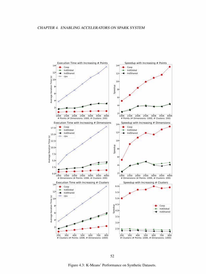
CHAPTER 4. ENABLING ACCELERATORS ON SPARK SYSTEM
100K 150K 200K 250K 300K 350K 400K# Points (# Dimensions: 1000, # Clusters: 200)
2
4
6
8
10
12
14
Aver
age
Itera
tion
Tim
e (s
)
Execution Time with Increasing # PointsCoopIndGlobalIndSharedcpu
100K 150K 200K 250K 300K 350K 400K# Points (# Dimensions: 1000, # Clusters: 200)
2
4
6
8
10
12
14
Spee
dup
Speedup with Increasing # PointsCoopIndGlobalIndShared
1000 1500 2000 2500 3000 3500 4000# Dimensions (# Points: 100K, # Clusters: 200)
0.0
2.5
5.0
7.5
10.0
12.5
15.0
17.5
Aver
age
Itera
tion
Tim
e (s
)
Execution Time with Increasing # DimensionsCoopIndGlobalIndSharedcpu
1000 1500 2000 2500 3000 3500 4000# Dimensions (# Points: 100K, # Clusters: 200)
2
4
6
8
10
12
14
Spee
dup
Speedup with Increasing # DimensionsCoopIndGlobalIndShared
200 300 400 500 600 700 800# Clusters (# Points: 100K, # Dimensions: 1000)
2
4
6
8
10
12
14
Aver
age
Itera
tion
Tim
e (s
)
Execution Time with Increasing # ClustersCoopIndGlobalIndSharedcpu
200 300 400 500 600 700 800# Clusters (# Points: 100K, # Dimensions: 1000)
2.5
3.0
3.5
4.0
4.5
5.0
5.5
6.0
Spee
dup
Speedup with Increasing # Clusters
CoopIndGlobalIndShared
Figure 4.3: K-Means’ Performance on Synthetic Datasets.
52

CHAPTER 4. ENABLING ACCELERATORS ON SPARK SYSTEM
with increased k, thanks to its ability to skip distance calculations. In this category, Coop gradually
approaches to a 6x speedup.
4.3.3.2 Logistic Regression
To generate the datasets for logistic regression, we alternate between −1 and 1 n times,
and in each time period, a d-dimensional data point is generated following a multivariate normal
distribution whose mean is labeli ∗ 0.7. This produces a clear decision boundary for negative and
positive classes.
We conduct two sets of experiment while varying n and d for the data points. The execution
times for CPU are very similar when varying the n v.s. d, as can be seen on the left in Figure 4.4.
This is because that the computation bottleneck for CPU lies in the dot product of wTxi for all n data
points, which has a complexity of O(nd). Thus the execution time is only associated with the total
size of the data points n× d. Same complexity applies for the GPU algorithm, but since on GPUs
we conduct a matrix-vector multiplication XW , where multiple dot-product of wTxi are executed in
parallel, we achieve a much better performance with up to 9x speedup.
4.3.3.3 Page Rank
The datasets for page rank is simply generated by randomly selecting (i, j) pairs to represent
the links from page j to page i in the adjacency matrix A. These pairs are then pre-processed to
generate two different formats for the Spark CPU and the Spark GPU implementations. For Spark
CPU, the input file contains lines of [pagei: outlink1, outlink2, ... ], while for the Spark GPU
implementation, we use a sparse matrix format where each line is [i, j, aij].
We conduct two experiments, where we either change the number of pages n, or the
number of links. As shown in Figure 4.5, the execution time of PageRank calculation on Spark CPU
generally grows linearly with the number of links, and does not change much with increasing number
of pages. However, on Spark GPU, this is a different story. There is not an obvious pattern with
either increased number of links or number of pages. The speedup from GPU ranges from 2.5x to
5.5x.
This is because SpMV is highly dependent on the distribution of the non-zero elements
in each row, with our randomly generated non-zero entries, the performance result does not have a
pattern.
53

CHAPTER 4. ENABLING ACCELERATORS ON SPARK SYSTEM
100K 150K 200K 250K 300K 350K 400K# Points (# Dimensions: 1000)
0.2
0.4
0.6
0.8
1.0
1.2
1.4
1.6
Aver
age
Itera
tion
Tim
e (s
)
Execution Time with Increasing # Pointsgpucpu
100K 150K 200K 250K 300K 350K 400K# Points (# Dimensions: 1000)
4.5
5.0
5.5
6.0
6.5
7.0
7.5
8.0
Spee
dup
Speedup with Increasing # Pointsgpu
1000 1500 2000 2500 3000 3500 4000# Dimensions (# Points: 100K)
0.2
0.4
0.6
0.8
1.0
1.2
1.4
1.6
Aver
age
Itera
tion
Tim
e (s
)
Execution Time with Increasing # Dimensionsgpucpu
1000 1500 2000 2500 3000 3500 4000# Dimensions (# Points: 100K)
5
6
7
8
9
Spee
dup
Speedup with Increasing # Dimensionsgpu
Figure 4.4: Logistic Regression’s Performance on Synthetic Datasets.
54

CHAPTER 4. ENABLING ACCELERATORS ON SPARK SYSTEM
100M 200M 300M 400M# Links (# Pages: 200K)
10
20
30
40
50
60
Aver
age
Itera
tion
Tim
e (s
)
Execution Time with Increasing # Linksgpucpu
100M 200M 300M 400M# Links (# Pages: 200K)
2.5
3.0
3.5
4.0
4.5
5.0
5.5
Spee
dup
Speedup with Increasing # Linksgpu
200K 400K 600K 800K 1000K# Pages (# Links: 200M)
5
10
15
20
25
Aver
age
Itera
tion
Tim
e (s
)
Execution Time with Increasing # Pagesgpucpu
200K 400K 600K 800K 1000K# Pages (# Links: 200M)
2.5
3.0
3.5
4.0
4.5
5.0
Spee
dup
Speedup with Increasing # Pagesgpu
Figure 4.5: Page Rank’s Performance on Synthetic Datasets.
55

Chapter 5
Sparkculator
As discussed in previous chapters, there is a lack of ML libraries running on GPU-enabled
Spark, and there is a a lack of user-friendly middleware that integrates GPU power with Spark’s
distributed infrastructure. Though GPUEnabler provides an opportunity to address these two issues,
it is hindered by its complicated programming interface, inefficient memory management, and lack
of support for various data types. Learning from the experiences gained by extending GPUEnabler,
we propose Sparkculator (Spark CUDA Accelerator), a novel GPU-integrated Spark framework
built from the ground up. The framework provides two interfaces — 1) a user interface, and
2) a developer interface. The user interface is an (ML) library that enables ML practitioners to
accelerate their data analytics tasks without any knowledge of the underlying GPUs; and the developer
interface is to help experienced GPU programmers to fully utilize the GPU’s power by effortlessly
integrating finely-tuned GPU kernels to Spark, and as a result, expand the ML library by adding
more optimized ML applications. We strive to maintain a clean API that retains as much similarity to
Spark as possible. The user interface is exactly the same as that of Spark; the developer interface
requires only a few additional lines of Sparkculator-specific code that glues the Spark and GPU
runtimes together. Similar to SWAT, we develop Sparkculator without modifying Spark’s core code,
making it a plug-in software, maintaining a high degree of compatibility with actively updated Spark
projects. Sparkculator supports a wide range of data structures, including primitive arrays from
Scala, dense vectors and sparse vectors from Breeze [69] and MLlib [48], as well as composite
types that dynamically bind together different data types. We have developed a ML library based on
Sparkculator and conduct an extensive performance evaluation on these ML algorithms.
Figure 5.1 presents the design of Sparkculator. In this chapter, we start by describing
Sparkculator’s user interface, and then we delve into each layer, detailing how each component
56
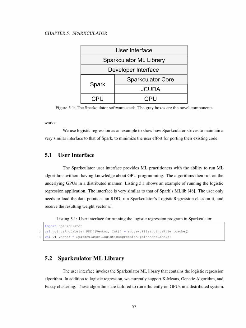
CHAPTER 5. SPARKCULATOR
Figure 5.1: The Sparkculator software stack. The gray boxes are the novel components
works.
We use logistic regression as an example to show how Sparkculator strives to maintain a
very similar interface to that of Spark, to minimize the user effort for porting their existing code.
5.1 User Interface
The Sparkculator user interface provides ML practitioners with the ability to run ML
algorithms without having knowledge about GPU programming. The algorithms then run on the
underlying GPUs in a distributed manner. Listing 5.1 shows an example of running the logistic
regression application. The interface is very similar to that of Spark’s MLlib [48]. The user only
needs to load the data points as an RDD, run Sparkculator’s LogisticRegression class on it, and
receive the resulting weight vector ~w.
Listing 5.1: User interface for running the logistic regression program in Sparkculator
1 import Sparkculator
2 val pointsAndLabels: RDD[(Vector, Int)] = sc.textFile(pointsFile).cache()
3 val w: Vector = Sparkculator.LogisticRegression(pointsAndLabels)
5.2 Sparkculator ML Library
The user interface invokes the Sparkculator ML library that contains the logistic regression
algorithm. In addition to logistic regression, we currently support K-Means, Genetic Algorithm, and
Fuzzy clustering. These algorithms are tailored to run efficiently on GPUs in a distributed system.
57

CHAPTER 5. SPARKCULATOR
GPU programmers can easily contribute to the library, adding applications using Sparkculator’s
developer interface, as described in the following section.
5.3 Developer Interface
To implement an ML algorithm in Sparkculator, GPU programmers need to write a Spark
program and a CUDA kernel, and integrate their CUDA code into Sparkculator using the developer
interface. GPUEnabler [24] inspires the design of the developer interface. Listing 5.2 shows the
source code for logistic regression using the developer interface. The main portion of the program
(line 12 to line 18) is the same as the Spark in Listing 1.1, with two exceptions:
• the replacement of map function to mapCUDA
• in addition to the lambda function f, mapF is also passed to mapCUDA
We will describe these two differences in the following sections.
Listing 5.2: Logistic Regression Program in Sparkculator
1 val mapParams = new ParamList(
2 InParam("pointsAndLabels", Cache, Transpose),
3 OutParam("gradients", Recycle, Transpose),
4 BroadcastParam("w", Recycle),
5 ConstParam("d"))
6 val redParams = new ParamList(
7 InParam("gradients")
8 OutputParam("gradient")
9 ConstParam("d"))
10 val mapF = new SparkcuFunc("genGrads", mapParams)
11 val redF = new SparkcuFunc("sumGrads", redParams)
12 for(i <-1 to ITERATIONS)
13 val gradients = points.mapCUDA(
14 p => f(p, w), mapF, w, d)
15 val gradient = gradients.reduceCUDA(
16 (g1, g2) => g1 + g2, redF, d)
17 w -= gradient
18
5.3.1 mapCUDA
Instead of applying a lambda function to every point in the RDD using map in Spark,
mapCUDA applies a CUDA kernel to a whole RDD partition, where the partition contains multiple
58
CHAPTER 5. SPARKCULATOR
points. A GPU works best when it is able to process a large chunk of consecutive data items using
thousands of threads. Given that the GPU is able to efficiently change threads in a single cycle,
executing a very large number of threads allows the GPU to hide memory latency, and amortize the
cost of context creation and kernel invocation. This approach to performance is quite different from
Spark’s iterator-based processing model, where a CPU core processes one data item at a time. To
ensure compatibility with Spark, the runtime in Sparkculator extends the iterator pattern so that a
standard Spark CPU task can be pipelined after a Sparkculator’s GPU task.
5.3.2 SparkcuFunc
mapF, defined at Line 10, is an object of class SparkcuFunc. SparkcuFunc is a wrapper
that encloses all the information to launch a CUDA kernel, including
1. kernel function’s name, e.g., “genGrads” at line 10.
2. kernel function’s signature, defined by the class ParamList.
At Line 1, the mapParams specifies the paramter list for the mapF object. This includes
the input RDD “pointsAndLabels”, the output RDD “gradients”, the broadcast data “w”, and the
constant paramter “d”(the dimension of the data point). Programmers can specify how they want to
persist the data on GPU memory with three options:
• Cache: this option caches the data on a GPU’s device memory; it is very efficient for read-only
data that is repeatedly accessed, such as the points and the labels in logistic regression.
• Recycle: this option denotes that the allocated GPU buffer does not need to be freed after the
kernel completion, and the contents of the buffer can be overwritten. We use this option for
the output buffer that stores all of the gradients, which are updated in each iteration.
• NoCache: this is the default option, which informs the runtime to free GPU memory after the
kernel completion.
Besides the caching options, developers can also indicate if they want to transpose a buffer
before it is copied to the GPU, which is useful for creating coalesced memory access for threads on
the GPU. The memory system on most GPUs contain a coalescing unit, able to collapse many (up to
32 on an NVIDIA GPU) spatially local accesses into a single memory system access [70].
59

CHAPTER 5. SPARKCULATOR
The developer interface incurs minimal changes as compared to a standard Spark program.
To write the corresponding CUDA program, the developer can conveniently follow the exact order of
the parameters in the ParamList, which makes it convenient to write error-free code. The CUDA
kernel for the map function is shown as follows:
__global__ genGrads(double* points,
int* labels,
double* gradients,
double* w,
int d,
int size)
Note that the RDD pointsAndLabels is de-coupled into two separate primitive arrays,
and size is a variable that is automatically added by Sparkculator which indicates the number of
data items in the partition this kernel function is invoked on.
5.4 Sparkculator Core
The Sparkculator core serves as the communication layer between Spark and a GPU. The
SparkcuFunc objects and RDD defined in the upper layers are relayed to the Sparkculator core,
which then offloads them as CUDA functions and native data buffers to the GPU using JCUDA [57].
We describe how to offload the CUDA function and data to the GPUs in the following sections.
5.4.1 Offloading CUDA Functions to GPUs
The SparkcuFunc described previously, encapsulates all the meta information needed to
launch a GPU kernel in the native CUDA environment, including the kernel source code, parameter
and grid/block configurations, and shared memory size. When we start a Sparkculator job, a
SparkcuFunc object is created as a broadcast variable that is shared by every worker node.
5.4.2 Offloading Spark Data to GPUs
A typical Spark framework and a GPU manage memory in two very different ways. Spark’s
RDD, broadcast data, and result data are all located on the heap memory, managed by the Java
Virtual Machine (JVM). Spark users do not need to worry about the layout of the data. They do not
worry if data is stored consecutively in memory, or if a matrix should be accessed in row-major or
column-major order. Neither do they care about how to de-allocate the data, as the JVM’s garbage
60

CHAPTER 5. SPARKCULATOR
collector automatically handles this. On the other hand, GPU programmers need to take care of
managing two types of off-heap memory — the system memory associated with the CPU, and the
device memory on the GPU. The memory layout and de-allocation are both manually managed by
the GPU programmer, and utilizing the right layout for the data can make a huge difference in overall
performance. To manage these different types of buffers, we have developed SparkcuBuffer,
a versatile class that manages data buffers in four different memory spaces — 1) on-heap memory,
2) off-heap system memory, 3) GPU global memory, and 4) GPU shared memory. Figure 5.2
shows an example of how SparkcuBuffer stores different types of data, including the input RDD
poinstAndLabels, the broadcast data ~w, and the output RDD gradients.
pointsAndLabels is of composite Tuple2 type (Vector, Int)when it is stored on
the heap as a standard RDD. SparkcuBuffer supports a wide range of data types, including primitive
scalars, primitive arrays, DenseVector, SparseVector from Breeze [69] and Spark’s MLlib [48], as
well as composite types such as Tuple2 that binds the types mentioned above together. For this
Tuple2 type, Sparkculator dynamically infers the type and transfers the data to two off-heap buffers,
where both points and labels are stored as a primitive array, in a piece of page-locked, consecutive,
memory. The points data is transposed if the transpose flag is set in the mapParams, as discussed
in Section 5.3.2. The transformed buffer is then transferred to GPU’s global memory asynchronously
using CUDA streams. Because the pointsAndLabels object is rather large, and thus cannot fit
into the shared memory, the data transfer stops at the global memory level; for smaller data structures
that need repeated data accesses such as the weight vector ~w, we transfer them to shared memory to
significantly reduce access latency. As for the output buffer gradients, we map it to GPU global
memory. The output buffer is populated after kernel completion. However, instead of promptly
transferring it to the heap memory, we keep it in device memory. We discuss this lazy evaluation
model in the next section.
5.4.3 Buffer Caching and Lazy Evaluation
We use the lineage graph shown in Figure 5.3 to illustrate how Sparkculator efficiently
manages different buffers by deploying a caching and lazy evaluation mechanism. After the RDD
points is loaded from storage data pointsFile, it is then transformed and transferred to the
system’s off-heap memory, and later transferred to global memory and marked as cached (indicated
by a shaded box).
The broadcast data weight vector ~w is first initialized as a random vector, and then
61

CHAPTER 5. SPARKCULATOR
Figure 5.2: Input, broadcast, and output SparkcuBuffers, an arrow indicates a data transfer direction
from one memory space to another.
transferred all the way to the global memory. When the kernel is launched, ~w is copied to the shared
memory, as it is accessed multiple time during kernel execution. Note that a dashed box indicates that
the buffer is to be recycled, i.e., it is a read-write buffer whose contents can be overwritten, though
should not be de-allocated since this would be inefficient. Recycled buffers are generally useful for
managing broadcast variables which are overwritten in each iteration, but retain the same data types
and sizes.
We also utilize a lazy evaluation mechanism for managing buffers. For input and broadcast
buffers, we do not copy the data to GPU’s device memory until a CUDA kernel using these buffers
is launched. For output buffers, we only allocate them in global memory. After kernel completion
when the buffer is populated, we do not promptly transfer it back to the on-heap memory (i.e., we
transfer it lazily). For example, in Figure 5.3, the device buffer gradients is the output buffer of
the kernel “genGrads” and the input buffer for kernel “sumGrads”. The contents of the buffer is never
needed by any CPU operation, therefore keeping it on the device memory reduces three expensive
operations: 1) the transfer from the GPU’s device memory to the CPU’s off-heap memory, 2) the
data transpose, and 3) the transfer from off-heap to on-heap memory. Output buffers implement the
Iterator interface, and we transfer the buffer up to the on-heap memory only when next() or
hasNext() are invoked. For example, in Figure 5.3, one gradient buffer is generated on the
GPU on each worker node, which needs to be returned to the driver node for a reduction operation to
62

CHAPTER 5. SPARKCULATOR
Figure 5.3: Lineage graph for 2 iterations of logistic regression in Sparkculator, a Sparkculator buffer
contains at most four different types of memory: RDD, CPU off-heap, GPU global, and GPU shared
update ~w. This reduction operation calls hasNext() of the buffer’s Iterator interface, which
triggers the memory copy process.
When the updated ~w is generated, the following iterations execute much faster than the
first iteration due to two main reasons: 1) the data points are cached in global memory, and 2) W1,
gradients, and gradient are all recycled buffers – they are pre-allocated in the first iteration
and do not need to be re-allocated or de-allocated in the following iterations.
Our buffer caching and lazy evaluation model significantly improve Sparkculator’s effi-
ciency and performance. The programmer only need to use the Cache/Recycle/NoCache flag, and
Sparkculator automatically does the remaining work.
5.5 Performance Evaluation
In this section, we present a comprehensive performance evaluation of our GPU-enabled
Sparkculator framework using four machine learning workloads currently supported in Sparkculator’s
ML library. To compare Sparkculator with Spark, we have also developed corresponding Spark-
CPU implementations to serve as our performance baseline. We strive to maintain a competitive
Spark-CPU baseline by offloading linear algebra operations to low-level BLAS routines, using the
netlib-java [71] library. We conduct our experiments on Amazon EC2 instances, and run applications
63
CHAPTER 5. SPARKCULATOR
using large, real world, datasets. We first study the overall performance and scalability of Sparkculator
versus Spark. Then we present an execution time breakdown for each application to better explain
the sources of overall performance benefits.
5.5.1 Experimental Setup
We use the same experimental setup as the one discussed in Section 4.3.2. The datasets are
initially cached in system memory on each node. Because all benchmarks are iterative algorithms,
we let each application run 5 iterations and extract the mean execution time per iteration.
5.5.2 Benchmarks and Datasets
We use four benchmarks to evaluate Sparkculator:
• Logistic Regression (LR): This is the example classification algorithm we use throughout the
thesis. We offload both the n gradient vector calculations and the summations to the GPU.
• KMeans: An iterative clustering algorithm. After the initial k cluster centroids are selected, the
algorithm consists of two major stages: 1) the labeling stage: this stage calculates nk distances
of each data point xi ∈ Rd to each cluster centroid cj , and selects the centroid with the smallest
distance as the new cluster label for each data point; the complexity of the labeling stage is
O(ndk). 2) the updating stage: this stage regenerates a new set of centroids by computing the
mean of all data points in the same cluster. This stage’s complexity is only O(nd), which is
much lower than that in the labeling stage. As a result, we only offload the labeling stage to
the GPU.
• Fuzzy: A soft clustering method. Similar to KMeans, it includes labeling and updating stages.
However, the complexity of both stages is higher in Fuzzy. The labeling stage first calculates
nk distances, but instead of selecting just one centroid for each data point, it creates an n× kpartition matrix P , where Pij indicates the degree to which the data point xi belongs to the
cluster cj . As a result, the complexity of the labeling stage in Fuzzy is O(ndk2). In the
updating stage, because each xi belongs to all k centers, the complexity becomes O(ndk). In
our implementation, we only offload the labeling stage to the GPU; we discuss the reasons for
this choice later in the thesis.
• Genetic Algorithm (GA): a type of evolutionary algorithm that iteratively updates the features
of a dataset by using biology-inspired operations such as mutation, crossover, and selection.
64

CHAPTER 5. SPARKCULATOR
We offload the selection step to the GPU, where the fitness function is evaluated for each
individual data point. GA is different from the other three algorithms as its data is overwritten
in each iteration. Therefore we use recycled buffers to store this data on the GPU.
The dataset we use to evaluate these workloads is the MNIST digits dataset [72]. The dataset provides
784 columns of features and 1 column of class labels. We use 1.8 million data points for LR and 3.5
million data points for the other three workloads. The input data for LR is smaller because it requires
twice as much GPU memory as the other benchmarks. The total amount of GPU memory needed
for each workload is approximately 20GB — the maximum amount of GPU memory when using
two nodes. Note that we use the same input data for 2, 4, and 8 nodes to evaluate Sparkculator’s
strong scaling behavior. During our experiments, we have also tested Sparkculator using synthetic
datasets and the Census dataset from the UCI Machine Learning Repository [73]; Sparkculator shows
consistent performance and scalability when using these datasets compared to the MNIST datasets.
5.5.3 Overall performance and scalability
Figure 5.4: Sparkculator’s overall speedup for each benchmark running on 2, 4, and 8 worker nodes.
Figure 5.4 shows the overall speedup generated by Sparkculator versus Spark. The
benchmarks achieve a speedup ranging from 3x to 8x. The amount of speedup achieved is correlated
65

CHAPTER 5. SPARKCULATOR
with the relative amount of work assigned to the GPU versus the CPU. LR achieves the best speedup
because it runs almost exclusively on the GPU. KMeans’s speedup is lower because only the labeling
stage is offloaded to the GPU, reducing the overall performance since both platforms execute the
updating stage on the CPU. GA runs the least on the GPU — only selection is performed on the
GPU. In addition, there is no caching of input data on the GPU for GA, as the data is updated in
every iteration, leaving GPU unoccupied.
Figure 5.5 presents the speedup achieved by both platforms when moving from 2 nodes to
4 nodes and 8 nodes. This illustrates the strong scaling behavior of both platforms. Both LR and GA
achieve linear or superlinear scalability on both CPU and GPU platforms (our CPU implementation
is scalable). KMeans and Fuzzy achieve rather low scalability because they have low resource
utilization, which we will discuss later in the thesis.
Figure 5.5: Speedup achieved when using 4 and 8 nodes versus 2 nodes on each platform.
5.5.4 Execution Time Breakdown
Next, we study detailed performance profiling data collected from selected benchmarks
to better understand the performance benefits produced by Sparkculator. Figure 5.6 shows LR’s
execution time breakdown for the CPU, and the components of GPU computation and GPU memory
66

CHAPTER 5. SPARKCULATOR
transfers, across 3 iterations on 2 worker nodes and 4 worker nodes. We can make two observations:
1) this application runs almost exclusively on the GPU, as the GPU data transfer and compute times
dominate the execution time, which explains why LR achieves the best overall speedup, 2) when we
increase the number of the nodes from 2 to 4, both GPU computation and memory transfer times are
reduced by more than half, because not only does each GPU get assigned only half the workload,
but the overhead to manage concurrent kernel execution and asynchronous CPU-to-GPU memory
transfers is also reduced. As a result, we achieve superlinear scaling when using 4 nodes.
Figure 5.6: CPU and GPU execution time breakdown for LR on 2 worker nodes versus 4 worker
nodes, across 3 iterations.
Figure 5.7 highlights the vastly different execution patterns present in KMeans, Fuzzy, and
GA. In KMeans, there are very few GPU memory transfers, as all the data points are cached on
the GPU, and only the clustering labels are sent back to the on-heap memory during each iteration.
However, the computational intensity in KMeans is very low — an iteration only takes about 1.2
seconds to complete. This short amount of execution time makes the data transfer time across
different nodes the main bottleneck, which explains the limited strong scaling of KMeans. Fuzzy has
a better GPU-to-CPU ratio because the labeling stage has much higher complexity (O(ndk2) versus
O(ndk) in KMeans, as discussed previously. However, as the GPU optimizes the labeling stage, the
overall performance is bottlenecked by the updating stage, which runs on the CPU. Even though
Fuzzy’s updating stage is data parallel and has rather high complexity (O(ndk)), we do not offload it
to the GPU because the updating stage has a unique buffer caching/recycling pattern. Both the input
67

CHAPTER 5. SPARKCULATOR
data point xi and its entry in the partition matrix Pi are needed to update the centroids, where xi is
a read-only buffer which can be cached on the GPU, and Pi is a read-write buffer which needs to
be updated on the GPU in each iteration. During runtime, Spark combines these two buffers into
an iterator of a composite type: Iterator[(xi, Pi)], so in order to extract every Pi buffer to
update the GPU memory, we need to iterate through each xi as well, which incurs the same amount of
on-heap memory access overhead as uncached data points. As a result, we only offload the labeling
stage and leave optimization of on-heap memory accesses as the future work.
GA differs from KMeans in three respects: 1) it spends most of its time on GPU memory
transfers, caused by frequent data point updates during each iteration, 2) even though GPU memory
transfers are long, GA is computationally heavy and data parallel, so it still obtains better overall
performance when running on GPUs versus CPUs. 3) each iteration for GA is much longer than
KMeans — usually around 20 seconds, which can help amortize the cross-network overhead, leading
to much better scalability.
Figure 5.7: CPU and GPU execution time breakdown for KMeans, Fuzzy and GA on 2 worker nodes,
across 3 iterations.
68

Chapter 6
Conclusion
To summarize, our work has made several contributions:
• We identify and analyze the data-parallel characteristics of general machine learning algorithms,
which can be mapped to multiple GPUs on multiple worker nodes in a distributed system, to
utilize the task-level and thread-level parallelism.
• We implement a Hadoop-based recommender system using GPUs and evaluate the perfor-
mance [74, 75].
• We extend GPUEnabler and build a distributed computing framework that effectively utilizes
GPUs on each computing node. We use this framework to study the performance characteristics
of different ML algorithms and evaluate its performance and scalability on AWS, where we
obtain promising performance gains [76].
• From the experiences learned from extending GPUEnabler, we build Sparkculator [77], an
GPU-enabled Spark system, from the ground up. Sparkculator provides a clean user-interface
and efficient runtime, and fundamentally solves the issues we encountered in extending
GPUEnabler.
• We build an ML library based on Sparkculator, which provides ML practitioners to fast deploy
their ML tasks, we also build a developer interface, which enables GPU experts to fully utilize
the GPU power by continently plug their fine-tuned GPU kernel programs into Spark’s runtime.
• We also evaluate Sparkculator using our ML library with real-world datasets on AWS, and
obtain 4x to 8x speedups for all applications.
69
CHAPTER 6. CONCLUSION
6.1 Future Research Directions
We plan to extend this work by adding more general-purpose ML algorithms to the
framework. We would prefer adding more generic ML algorithms, such as stochastic gradient descent,
that are often used as building blocks for other more sophisticated algorithms. The acceleration of
such algorithms would benefit more ML researchers and data scientists. Adding more benchmarks
would also help us explore a larger design space to evaluate and improve the framework’s efficiency.
As discussed in our analysis of the Fuzzy clustering algorithm, we would like to improve the
performance of on-heap memory accesses when using composite data structures that do not share the
same caching/recycling properties. At last, we will look at the overall CPU/GPU resources utilization
on a worker node, to investigate further improving the framework’s efficiency and reduce node idling
time.
70

Bibliography
[1] A. Thusoo, J. S. Sarma, N. Jain, Z. Shao, P. Chakka, N. Zhang, S. Antony, H. Liu, and R. Murthy,
“Hive-a petabyte scale data warehouse using hadoop,” in Data Engineering (ICDE), 2010 IEEE
26th International Conference on. IEEE, 2010, pp. 996–1005.
[2] J. Dean and S. Ghemawat, “Mapreduce: simplified data processing on large clusters,”
Commun. ACM, vol. 51, no. 1, pp. 107–113, Jan. 2008. [Online]. Available:
http://doi.acm.org/10.1145/1327452.1327492
[3] T. Chen, M. Li, Y. Li, M. Lin, N. Wang, M. Wang, T. Xiao, B. Xu, C. Zhang, and Z. Zhang,
“Mxnet: A flexible and efficient machine learning library for heterogeneous distributed systems,”
arXiv preprint arXiv:1512.01274, 2015.
[4] E. P. Xing, Q. Ho, W. Dai, J. K. Kim, J. Wei, S. Lee, X. Zheng, P. Xie, A. Kumar, and Y. Yu,
“Petuum: A new platform for distributed machine learning on big data,” IEEE Transactions on
Big Data, vol. 1, no. 2, pp. 49–67, 2015.
[5] “Apache hadoop website,” http://hadoop.apache.org/.
[6] M. Zaharia, M. Chowdhury, T. Das, and A. Dave, “Resilient distributed datasets: A
fault-tolerant abstraction for in-memory cluster computing,” NSDI’12 Proceedings of the 9th
USENIX conference on Networked Systems Design and Implementation, pp. 2–2, 2012. [Online].
Available: https://www.usenix.org/system/files/conference/nsdi12/nsdi12-final138.pdf
[7] M. Odersky and al., “An Overview of the Scala Programming Language,” EPFL, Lausanne,
Switzerland, Tech. Rep. IC/2004/64, 2004.
[8] R. Raina, A. Madhavan, and A. Y. Ng, “Large-scale deep unsupervised learning using graphics
processors,” in Proceedings of the 26th Annual International Conference on Machine Learning
71

BIBLIOGRAPHY
- ICML ’09. New York, New York, USA: ACM Press, 2009, pp. 1–8. [Online]. Available:
http://portal.acm.org/citation.cfm?doid=1553374.1553486
[9] N. Bell and M. Garland, “Implementing sparse matrix-vector multiplication on throughput-
oriented processors,” Proceedings of the Conference on High Performance Computing
Networking, Storage and Analysis - SC ’09, no. 1, p. 1, 2009. [Online]. Available:
http://dl.acm.org/citation.cfm?doid=1654059.1654078
[10] A. Coates, B. Huval, T. Wang, D. Wu, and A. Y. Ng, “Deep learning with COTS HPC systems,”
Proceedings of The 30th International Conference on Machine Learning, pp. 1337–1345, 2013.
[11] F. Azmandian, A. Yilmazer, J. Dy, J. Aslam, and D. Kaeli, “GPU-accelerated feature selection
for outlier detection using the local kernel density ratio,” in Proceedings of the IEEE 12th
International Conference on Data Mining (ICDM), 2012, pp. 51–60.
[12] W.-m. W. Hwu, GPU Computing Gems Emerald Edition, 1st ed. San Francisco, CA, USA:
Morgan Kaufmann Publishers Inc., 2011.
[13] R. Farivar, D. Rebolledo, E. Chan, and R. H. Campbell, “A parallel implementation of k-means
clustering on gpus.” in Pdpta, vol. 13, no. 2, 2008, pp. 212–312.
[14] K. J. Kohlhoff, V. S. Pande, and R. B. Altman, “K-means for parallel architectures using
all-prefix-sum sorting and updating steps,” IEEE Transactions on Parallel and Distributed
Systems, vol. 24, no. 8, pp. 1602–1612, 2013.
[15] M. Zechner and M. Granitzer, “Accelerating k-means on the graphics processor via cuda,” in
Intensive Applications and Services, 2009. INTENSIVE’09. First International Conference on.
IEEE, 2009, pp. 7–15.
[16] Y. Liang, M.-F. Balcan, and V. Kanchanapally, “Distributed pca and k-means clustering,” in
The Big Learning Workshop at NIPS, vol. 2013, 2013.
[17] C. T. Chu, S. K. Kim, Y. A. Lin, Y. Yu, G. R. Bradski, A. Y. Ng, and
K. Olukotun, “Map-reduce for machine learning on multicore,” in NIPS, B. Schölkopf,
J. C. Platt, and T. Hoffman, Eds. MIT Press, 2006, pp. 281–288. [Online]. Available:
http://dblp.uni-trier.de/rec/bibtex/conf/nips/ChuKLYBNO06
72

BIBLIOGRAPHY
[18] Y. Low, J. Gonzalez, A. Kyrola, D. Bickson, C. Guestrin, and J. M. Hellerstein,
“Distributed GraphLab: A Framework for Machine Learning in the Cloud,” The 38th
International Conference on Very Large Data Bases, vol. 5, no. 8, pp. 716–727, 2012.
[Online]. Available: http://arxiv.org/abs/1204.6078%5Cnhttp://dl.acm.org/citation.cfm?id=
2212354http://arxiv.org/abs/1107.0922http://arxiv.org/abs/1204.6078
[19] A. Ghoting, R. Krishnamurthy, E. Pednault, B. Reinwald, V. Sindhwani, S. Tatikonda, Y. Tian,
and S. Vaithyanathan, “SystemML: Declarative machine learning on MapReduce,” in Proceed-
ings - International Conference on Data Engineering, 2011, pp. 231–242.
[20] A. M. Aji, J. Dinan, D. Buntinas, P. Balaji, W. C. Feng, K. R. Bisset, and R. Thakur, “MPI-ACC:
An integrated and extensible approach to data movement in accelerator-based systems,” in
Proceedings of the 14th IEEE International Conference on High Performance Computing and
Communications, HPCC-2012 - 9th IEEE International Conference on Embedded Software
and Systems, ICESS-2012, 2012, pp. 647–654.
[21] A. M. Aji, J. Mellor-Crummey, X. Ma, R. Thakur, L. S. Panwar, F. Ji, M. Chabbi, K. Murthy,
P. Balaji, K. R. Bisset, J. Dinan, and W.-c. Feng, “On the efficacy of GPU-integrated
MPI for scientific applications,” in Proceedings of the 22nd international symposium on
High-performance parallel and distributed computing - HPDC ’13. ACM, 2013, p. 191.
[Online]. Available: http://dl.acm.org/citation.cfm?doid=2493123.2462915
[22] D. Komatitsch, G. Erlebacher, D. Göddeke, and D. Michéa, “High-order finite-element seismic
wave propagation modeling with MPI on a large GPU cluster,” Journal of Computational
Physics, vol. 229, no. 20, pp. 7692–7714, 2010.
[23] T. M. Forum, “Mpi: A message passing interface,” 1993.
[24] K. Ishizaki and J. Samuel, “Gpuenabler github repository,” https://github.com/IBMSparkGPU/
GPUEnabler, 2016.
[25] D. Shreiner, G. Sellers, J. M. Kessenich, and B. M. Licea-Kane, OpenGL Programming Guide:
The Official Guide to Learning OpenGL, Version 4.3, 8th ed. Addison-Wesley Professional,
2013.
[26] F. Luna, Introduction to 3D Game Programming with DirectX 11. USA: Mercury Learning &
Information, 2012.
73
BIBLIOGRAPHY
[27] Intel, “8th generation intel core processor family datasheet,” https://www.intel.com/content/
www/us/en/processors/core/8th-gen-processor-family-s-platform-datasheet-vol-1.html.
[28] NVIDIA, “Nvidia tesla p100 gpu accelerator pcie datasheet,” http://images.nvidia.com/content/
tesla/pdf/nvidia-tesla-p100-PCIe-datasheet.pdf.
[29] “Nvidia website,” www.nvidia.com/.
[30] “Amd website,” www.amd.com/.
[31] C. Nvidia, “Cuda c programming guide,” 2017.
[32] A. Munshi, “The opencl specification,” in Hot Chips 21 Symposium (HCS), 2009 IEEE. IEEE,
2009, pp. 1–314.
[33] “Nvidia tegra gpus,” http://www.nvidia.com/object/tegra.html.
[34] “Amd apus,” http://www.amd.com/en/products/a-series-processors-desktop-7th-gen-fm2-plus.
[35] B. Gaster, L. Howes, D. Kaeli, P. Mistry, and D. Schaa, Heterogeneous computing with OpenCL,
2nd Edition. Morgan Kaufmann, 2011.
[36] “Chronos group,” https://www.khronos.org/.
[37] B. Catanzaro, N. Sundaram, and K. Keutzer, “A map reduce framework for programming
graphics processors,” in In Workshop on Software Tools for MultiCore Systems, 2008. [Online].
Available: http://citeseerx.ist.psu.edu/viewdoc/summary?doi=10.1.1.141.1644
[38] C.-C. Chang and C.-J. Lin, “Libsvm: a library for support vector machines,” ACM transactions
on intelligent systems and technology (TIST), vol. 2, no. 3, p. 27, 2011.
[39] B. He, W. Fang, Q. Luo, N. K. Govindaraju, and T. Wang, “Mars: A mapreduce framework
on graphics processors,” in Proceedings of the 17th International Conference on Parallel
Architectures and Compilation Techniques, ser. PACT ’08. New York, NY, USA: ACM, 2008,
pp. 260–269. [Online]. Available: http://doi.acm.org/10.1145/1454115.1454152
[40] C. Ranger, R. Raghuraman, A. Penmetsa, G. Bradski, and C. Kozyrakis, “Evaluating MapRe-
duce for multi-core and multiprocessor systems,” Proceedings - International Symposium on
High-Performance Computer Architecture, pp. 13–24, 2007.
74
BIBLIOGRAPHY
[41] C. Hong, D. Chen, W. Chen, W. Zheng, and H. Lin, “Mapcg: Writing parallel program
portable between cpu and gpu,” in Proceedings of the 19th International Conference on
Parallel Architectures and Compilation Techniques, ser. PACT ’10. New York, NY, USA:
ACM, 2010, pp. 217–226. [Online]. Available: http://doi.acm.org/10.1145/1854273.1854303
[42] J. A. Stuart and J. D. Owens, “Multi-gpu mapreduce on gpu clusters,” in Proceedings of
the 2011 IEEE International Parallel & Distributed Processing Symposium, ser. IPDPS ’11.
Washington, DC, USA: IEEE Computer Society, 2011, pp. 1068–1079. [Online]. Available:
http://dx.doi.org/10.1109/IPDPS.2011.102
[43] M. Grossman, M. Breternitz, and V. Sarkar, “HadoopCL: MapReduce on distributed
heterogeneous platforms through seamless integration of hadoop and OpenCL,” Pro-
ceedings - IEEE 27th International Parallel and Distributed Processing Symposium
Workshops and PhD Forum, IPDPSW 2013, pp. 1918–1927, may 2013. [On-
line]. Available: http://ieeexplore.ieee.org/lpdocs/epic03/wrapper.htm?arnumber=6651095http:
//dx.doi.org/10.1109/IPDPSW.2013.246
[44] G.Frost, “Aparapi website,” https://github.com/aparapi/aparapi.
[45] M. Grossman, M. Breternitz, and V. Sarkar, “HadoopCL2: Motivating the Design of a Dis-
tributed, Heterogeneous Programming System with Machine-Learning Applications,” IEEE
Transactions on Parallel and Distributed Systems, vol. 27, no. 3, pp. 762–775, 2016.
[46] S. Owen, R. Anil, T. Dunning, and E. Friedman, Mahout in Action, 1st ed. Manning
Publications Co. 20 Baldwin Road PO Box 261 Shelter Island, NY 11964: Manning
Publications Co., 2011. [Online]. Available: http://manning.com/owen/
[47] M. Grossman and V. Sarkar, “Swat: A programmable, in-memory, distributed, high-
performance computing platform,” in Proceedings of the 25th ACM International Symposium on
High-Performance Parallel and Distributed Computing, ser. HPDC ’16. New York, NY, USA:
ACM, 2016, pp. 81–92. [Online]. Available: http://doi.acm.org/10.1145/2907294.2907307
[48] X. Meng, J. Bradley, B. Yavuz, E. Sparks, S. Venkataraman, D. Liu, J. Freeman, D. Tsai,
M. Amde, S. Owen, D. Xin, R. Xin, M. J. Franklin, R. Zadeh, M. Zaharia, and A. Talwalkar,
“Mllib: Machine learning in apache spark,” J. Mach. Learn. Res., vol. 17, no. 1, pp. 1235–1241,
Jan. 2016. [Online]. Available: http://dl.acm.org/citation.cfm?id=2946645.2946679
75
BIBLIOGRAPHY
[49] “Apache mahout website,” http://mahout.apache.org/.
[50] G. Linden, B. Smith, and J. York, “Amazon.com recommendations: item-to-item collaborative
filtering,” Internet Computing, IEEE, vol. 7, no. 1, pp. 76–80, Jan 2003.
[51] J. Bennett and S. Lanning, “The netflix prize,” in Proceedings of KDD cup and workshop, vol.
2007, 2007, p. 35.
[52] J. A. Konstan, B. N. Miller, D. Maltz, J. L. Herlocker, L. R. Gordon, and J. Riedl, “Grouplens:
Applying collaborative filtering to usenet news,” Commun. ACM, vol. 40, no. 3, pp. 77–87, Mar.
1997. [Online]. Available: http://doi.acm.org/10.1145/245108.245126
[53] B. Sarwar, G. Karypis, J. Konstan, and J. Riedl, “Item-based collaborative filtering
recommendation algorithms,” in Proceedings of the 10th International Conference on World
Wide Web, ser. WWW ’01. New York, NY, USA: ACM, 2001, pp. 285–295. [Online].
Available: http://doi.acm.org/10.1145/371920.372071
[54] Y. Koren, R. Bell, and C. Volinsky, “Matrix factorization techniques for recommender systems,”
Computer, no. 8, pp. 30–37, 2009.
[55] D. A. Alcantara, V. Volkov, S. Sengupta, M. Mitzenmacher, J. D. Owens, and N. Amenta,
“Building an efficient hash table on the GPU,” in GPU Computing Gems, W. W. Hwu, Ed.
Morgan Kaufmann, Oct. 2011, vol. 2, ch. 4, pp. 39–53.
[56] G. E. Blelloch, “Prefix sums and their applications,” School of Computer Science, Carnegie
Mellon University, Tech. Rep. CMU-CS-90-190, Nov. 1990.
[57] Y. Yan, M. Grossman, and V. Sarkar, “Jcuda: A programmer-friendly interface for accelerating
java programs with cuda,” in Proceedings of the 15th International Euro-Par Conference
on Parallel Processing, ser. Euro-Par ’09. Berlin, Heidelberg: Springer-Verlag, 2009, pp.
887–899. [Online]. Available: http://dx.doi.org/10.1007/978-3-642-03869-3_82
[58] S. Liang, Java Native Interface: Programmer’s Guide and Reference, 1st ed. Boston, MA,
USA: Addison-Wesley Longman Publishing Co., Inc., 1999.
[59] D. Aloise, A. Deshpande, P. Hansen, and P. Popat, “Np-hardness of euclidean sum-of-squares
clustering,” vol. 75, pp. 245–248, 05 2009.
76

BIBLIOGRAPHY
[60] D. Arthur and S. Vassilvitskii, “k-means++: The advantages of careful seeding,” in Proceedings
of the eighteenth annual ACM-SIAM symposium on Discrete algorithms. Society for Industrial
and Applied Mathematics, 2007, pp. 1027–1035.
[61] B. Bahmani, B. Moseley, A. Vattani, R. Kumar, and S. Vassilvitskii, “Scalable k-means++,”
Proceedings of the VLDB Endowment, vol. 5, no. 7, pp. 622–633, 2012.
[62] J. Wu and B. Hong, “An efficient k-means algorithm on cuda,” in 2011 IEEE International
Symposium on Parallel and Distributed Processing Workshops and Phd Forum, May 2011, pp.
1740–1749.
[63] L. Page, S. Brin, R. Motwani, and T. Winograd, “The PageRank Citation Ranking: Bringing
Order to the Web,” World Wide Web Internet And Web Information Systems, vol. 54, no.
1999-66, pp. 1–17, 1998. [Online]. Available: http://ilpubs.stanford.edu:8090/422
[64] T. Wu, B. Wang, Y. Shan, F. Yan, Y. Wang, and N. Xu, “Efficient PageRank and SpMV
computation on AMD GPUs,” in Proceedings of the International Conference on Parallel
Processing, 2010, pp. 81–89.
[65] A. Rungsawang and B. Manaskasemsak, “Fast PageRank computation on a GPU cluster,” in
Proceedings - 20th Euromicro International Conference on Parallel, Distributed and Network-
Based Processing, PDP 2012, 2012, pp. 450–456.
[66] A. Ashari, N. Sedaghati, J. Eisenlohr, S. Parthasarathy, and P. Sadayappan, “Fast Sparse Matrix-
Vector Multiplication on GPUs for Graph Applications,” International Conference for High
Performance Computing, Networking, Storage and Analysis, SC, vol. 2015-Janua, no. January,
pp. 781–792, 2014.
[67] S. Sengupta, M. Harris, Y. Zhang, and J. D. Owens, “Scan primi-
tives for GPU computing,” Graphics . . . , pp. 97–106, 2007. [Online]. Avail-
able: http://portal.acm.org/citation.cfm?id=1280110%5Cnhttp://userweb.cs.utexas.edu/
users/pingali/CS378/2008sp/papers/ScanPrimitives.pdf
[68] S. Dalton, N. Bell, L. Olson, and M. Garland, “Cusp: Generic parallel algorithms
for sparse matrix and graph computations,” 2014, version 0.5.0. [Online]. Available:
http://cusplibrary.github.io/
[69] D. Hall and D. Ramage, “Breeze github repository,” https://github.com/scalanlp/breeze, 2009.
77

BIBLIOGRAPHY
[70] B. Jang, D. Schaa, P. Mistry, and D. Kaeli, “Exploiting memory access patterns to improve
memory performance in data-parallel architectures,” IEEE Trans. Parallel Distrib. Syst., vol. 22,
no. 1, pp. 105–118, Jan. 2011.
[71] S. Halliday, “netlib-java,” https://github.com/fommil/netlib-java, 2015.
[72] Y. LeCun, “The mnist database of handwritten digits,” http://yann. lecun. com/exdb/mnist/,
1998.
[73] D. Dheeru and E. Karra Taniskidou, “UCI machine learning repository,” 2017. [Online].
Available: http://archive.ics.uci.edu/ml
[74] X. Li, M. Grossman, and D. Kaeli, “Mahout on heterogeneous clusters using hadoopcl,”
in Proceedings of the 2nd Workshop on Parallel Programming for Analytics Applications,
ser. PPAA 2015. New York, NY, USA: ACM, 2015, pp. 9–16. [Online]. Available:
http://doi.acm.org/10.1145/2726935.2726940
[75] Y. Ukidave, X. Li, and D. Kaeli, “Mystic: Predictive scheduling for gpu based cloud
servers using machine learning,” in 2016 IEEE International Parallel and Distributed
Processing Symposium (IPDPS), vol. 00, May 2016, pp. 353–362. [Online]. Available:
doi.ieeecomputersociety.org/10.1109/IPDPS.2016.73
[76] Y. Sun, X. Gong, A. K. Ziabari, L. Yu, X. Li, S. Mukherjee, C. McCardwell, A. Villegas, and
D. Kaeli, “Hetero-mark, a benchmark suite for cpu-gpu collaborative computing,” in 2016 IEEE
International Symposium on Workload Characterization (IISWC). IEEE, 2016, pp. 1–10.
[77] X. Li and D. Kaeli, “Exploiting large-scale data analytics platforms with accelerator hardware,”
submitted to Big Data 2018.
78