exploring lora and lorawanpublications.lib.chalmers.se/records/fulltext/252610/252610.pdf ·...
TRANSCRIPT

Exploring LoRa and LoRaWANA suitable protocol for IoT weather stations?
Master’s thesis in Communication EngineeringKristoffer Olsson & Sveinn Finnsson
Department of Electrical EngineeringCHALMERS UNIVERSITY OF TECHNOLOGYGothenburg, Sweden 2017


Master’s thesis 2017:09
Exploring LoRa and LoRaWAN
A suitable protocol for IoT weather stations?
Kristoffer Olsson & Sveinn Finnsson
Department of Electrical EngineeringDivision of Communication and Antenna Systems
Chalmers University of TechnologyGothenburg, Sweden 2017
Exploring LoRa and LoRaWANA suitable protocol for IoT weather stations?Kristoffer Olsson & Sveinn Finnsson
© Kristoffer Olsson & Sveinn Finnsson, 2017.
Supervisors: Árni Alfreðsson, Electrical Engineering & Anders Olsson, ALTENSverigeExaminer: Erik Ström, Electrical Engineering
Master’s Thesis 2017:09Department of Electrical EngineeringDivision of Communication and Antenna SystemsChalmers University of TechnologySE-412 96 GothenburgTelephone +46 31 772 1000
Typeset in LATEXGothenburg, Sweden 2017
iv

Exploring LoRa and LoRaWANA suitable protocol for IoT Weather stations?Kristoffer Olsson & Sveinn FinnssonDepartment of Electrical EngineeringChalmers University of Technology
AbstractSvenska Sjöräddningssällskapet (SSRS) maintains a mobile-phone application thatprovides up-to-date weather information to seafarers in Sweden. In order to increasethe granularity of the weather data that powers the application, they wish to placesimple weather stations at popular sailing destinations in the archipelagos surround-ing Sweden.
In this thesis we examine a new radio protocol called LoRa and the accompany-ing low power wide area network protocol LoRaWAN. The aim of the thesis is toevaluate if and how these protocols can be used for the purpose of transmittingweather data from simple IoT weather stations. Furthermore, we wish to discussand present a specification to extend the effective range of the network.
The LoRa protocol is examined, along with the theory behind the chirp spreadspectrum modulation, which LoRa exploits. The network layer protocol LoRaWANand its structure is presented and shortly explained. We discuss how this struc-ture can be utilized for testing of the protocol and for our use-case. Furthermore,packet error rate testing is performed between an RN2483 transceiver and a Kerlinkgateway. Utilizing the results from this testing, we discuss and create a specificationfor network range extending intermediate-nodes. In addition to the specification, weprovide insight into suitable placement of the IoT weather stations and intermediate-nodes for good network coverage.
The LoRa protocol and the accompanying LoRaWAN network protocol is found tobe useful for the intended IoT weather stations. Furthermore, we find that our sug-gested network range extending specification is a good fit for the intended weatherstation network, but the intermediate-nodes introduce some limitations to the net-work when compared to gateways.
Keywords: LoRa, LoRaWAN, IoT, LPWAN, Weather, Station, Network, Extension.
v

AcknowledgementsWe thank ALTEN Sverige for supplying us with the problem presented in this thesisas well as the resources necessary for its fulfillment. Furthermore, we thank AndersOlsson at ALTEN Sverige for his guidance and support during the thesis. In addi-tion we thank our supervisor Árni Alfreðsson at Chalmers for providing us guidanceand assistance during our thesis project. We would also like to thank Patrik Sären-fors at Indesmatech (Semtech representative Nordic) for his support on making thegateway (Kerlink IoT station) function properly in mobile mode. Finally, we thankÞórhildur Hafsteinsdóttir for proof-reading the report and giving suggestions for im-proving it, and Karin Nylinder for her continuous support during the work on thethesis.
Kristoffer Olsson &Sveinn Finnsson, Gothenburg, September 2017
vii


Contents
List of Figures xiii
List of Tables xv
1 Introduction 11.1 SSRS & Alten . . . . . . . . . . . . . . . . . . . . . . . . . . . . . . . 11.2 Problem description . . . . . . . . . . . . . . . . . . . . . . . . . . . . 11.3 Thesis description . . . . . . . . . . . . . . . . . . . . . . . . . . . . . 2
2 LoRa and LoRaWAN 32.1 Other IoT protocols . . . . . . . . . . . . . . . . . . . . . . . . . . . . 32.2 LoRa . . . . . . . . . . . . . . . . . . . . . . . . . . . . . . . . . . . . 3
2.2.1 Basics of LoRa . . . . . . . . . . . . . . . . . . . . . . . . . . 42.2.2 LoRa - Chirp Spread Spectrum . . . . . . . . . . . . . . . . . 4
2.2.2.1 Coding scheme . . . . . . . . . . . . . . . . . . . . . 42.2.2.2 Achievable data rates . . . . . . . . . . . . . . . . . . 4
2.2.3 Key properties of LoRa . . . . . . . . . . . . . . . . . . . . . . 52.3 LoRaWAN . . . . . . . . . . . . . . . . . . . . . . . . . . . . . . . . . 5
2.3.1 Network topology . . . . . . . . . . . . . . . . . . . . . . . . . 62.3.2 Device classes . . . . . . . . . . . . . . . . . . . . . . . . . . . 72.3.3 Data rate and duty cycles . . . . . . . . . . . . . . . . . . . . 72.3.4 PHY and MAC layer structure . . . . . . . . . . . . . . . . . 8
2.3.4.1 PHY Message Formats . . . . . . . . . . . . . . . . . 82.3.4.2 MAC Message Formats . . . . . . . . . . . . . . . . 9
3 Theory 113.1 Spread Spectrum . . . . . . . . . . . . . . . . . . . . . . . . . . . . . 11
3.1.1 Spread spectrum and fading channel behavior . . . . . . . . . 113.1.2 Spread spectrum: frequency hopping and direct sequence . . . 12
3.2 Chirp Spread Spectrum . . . . . . . . . . . . . . . . . . . . . . . . . . 133.3 Line-of-sight and Fresnel zone clearance . . . . . . . . . . . . . . . . . 19
3.3.1 Line-of-sight . . . . . . . . . . . . . . . . . . . . . . . . . . . . 193.3.2 Fresnel zones . . . . . . . . . . . . . . . . . . . . . . . . . . . 20
4 Chip To Gateway Test 234.1 Purpose of Test . . . . . . . . . . . . . . . . . . . . . . . . . . . . . . 234.2 Related work . . . . . . . . . . . . . . . . . . . . . . . . . . . . . . . 23
ix

Contents
4.2.1 Theoretical performance . . . . . . . . . . . . . . . . . . . . . 234.2.2 Measured performance . . . . . . . . . . . . . . . . . . . . . . 26
4.3 Test parameters . . . . . . . . . . . . . . . . . . . . . . . . . . . . . . 274.4 Results . . . . . . . . . . . . . . . . . . . . . . . . . . . . . . . . . . . 294.5 Discussion of test results . . . . . . . . . . . . . . . . . . . . . . . . . 33
5 Network design 375.1 Considerations . . . . . . . . . . . . . . . . . . . . . . . . . . . . . . 37
5.1.1 Range of LoRa . . . . . . . . . . . . . . . . . . . . . . . . . . 375.1.2 Frequency Channel . . . . . . . . . . . . . . . . . . . . . . . . 375.1.3 Spreading Factor . . . . . . . . . . . . . . . . . . . . . . . . . 395.1.4 Message and Node Identification . . . . . . . . . . . . . . . . . 405.1.5 Acknowledgement of reception by intermediate node . . . . . . 405.1.6 Transmission protocol . . . . . . . . . . . . . . . . . . . . . . 405.1.7 Data transmission frequency . . . . . . . . . . . . . . . . . . . 415.1.8 Packet size from intermediate-node to Gateway . . . . . . . . 415.1.9 Security . . . . . . . . . . . . . . . . . . . . . . . . . . . . . . 425.1.10 Over The Air Updates . . . . . . . . . . . . . . . . . . . . . . 42
5.2 Network Extending Specification . . . . . . . . . . . . . . . . . . . . 425.2.1 Range of LoRa - Placement of nodes . . . . . . . . . . . . . . 425.2.2 Frequency Channel . . . . . . . . . . . . . . . . . . . . . . . . 435.2.3 Spreading Factor . . . . . . . . . . . . . . . . . . . . . . . . . 435.2.4 Message and Node Identification . . . . . . . . . . . . . . . . . 445.2.5 Acknowledgement of reception by intermediate node . . . . . . 445.2.6 Transmission protocol and Data transmission frequency . . . . 45
5.2.6.1 End-device to intermediate-node . . . . . . . . . . . 455.2.6.2 Intermediate-node to Gateway . . . . . . . . . . . . . 47
5.2.7 Security . . . . . . . . . . . . . . . . . . . . . . . . . . . . . . 475.2.8 Over The Air Updates . . . . . . . . . . . . . . . . . . . . . . 485.2.9 Connecting to and leaving LoRaWAN . . . . . . . . . . . . . 48
6 Discussion 496.1 LoRa and LoRaWAN . . . . . . . . . . . . . . . . . . . . . . . . . . . 49
6.1.1 LoRa . . . . . . . . . . . . . . . . . . . . . . . . . . . . . . . . 496.1.2 LoRaWAN . . . . . . . . . . . . . . . . . . . . . . . . . . . . . 49
6.2 Network extension specification vs. additional gateways . . . . . . . . 506.2.1 Advantages . . . . . . . . . . . . . . . . . . . . . . . . . . . . 506.2.2 Limitations . . . . . . . . . . . . . . . . . . . . . . . . . . . . 516.2.3 Suggested network extension specification changes for larger
networks . . . . . . . . . . . . . . . . . . . . . . . . . . . . . . 53
7 Conclusion 55
8 Future work 57
Bibliography 59
x

Contents
A Appendix 1 61
xi

Contents
xii

List of Figures
2.1 Uplink PHY structure . . . . . . . . . . . . . . . . . . . . . . . . . . 82.2 PHY Payload . . . . . . . . . . . . . . . . . . . . . . . . . . . . . . . 92.3 MAC Payload . . . . . . . . . . . . . . . . . . . . . . . . . . . . . . . 92.4 Frame header . . . . . . . . . . . . . . . . . . . . . . . . . . . . . . . 9
3.1 Illustration showing that when echoes from a sinusoidal pulse areproperly spaced in time, then each individual peak is clearly dis-cernible after matched filtering . . . . . . . . . . . . . . . . . . . . . . 15
3.2 Illustration showing that when echoes from a sinusoidal pulse areinterfering (i.e. not sufficiently apart in time), then the individualpeaks can not be distinguished after the matched filter output . . . . 16
3.3 Chirped signal and echo (a) and correlation of the two (b) . . . . . . 183.4 Fresnel zone height for different positions along 10 km communica-
tions link (a) and maximum Fresnel height for different link distances(b) . . . . . . . . . . . . . . . . . . . . . . . . . . . . . . . . . . . . . 21
4.1 Coverage probabilities for path loss exponents 2.4 through 2.7 aregiven in (a) - (d) for different spreading factors on a carrier frequencyof 868.5 MHz. Radio link distances varies from 0− 30 km . . . . . . . 26
4.2 The Kerlink LoRa IoT station positioned at lake Lygnern . . . . . . . 284.3 Comparison between the measured data (tables 4.4 - 4.7), fitted using
linear regression and the coverage probability from section 4.2.1 (usingpath loss exponent η = 2.4 and zoomed in accordingly) . . . . . . . . 32
5.1 Message format . . . . . . . . . . . . . . . . . . . . . . . . . . . . . . 455.2 Payload format . . . . . . . . . . . . . . . . . . . . . . . . . . . . . . 465.3 Intermediate-node frame format . . . . . . . . . . . . . . . . . . . . . 47
A.1 Histogram of RSSI for data collected at 1.0 km. . . . . . . . . . . . . 61A.2 Histogram of RSSI for data collected at 3.0 km. . . . . . . . . . . . . 61A.3 Histogram of RSSI for data collected at 5.0 km. . . . . . . . . . . . . 62A.4 Histogram of RSSI for data collected at 7.0 km. . . . . . . . . . . . . 62A.5 RSSI for data collected at 1.0 km. . . . . . . . . . . . . . . . . . . . . 63A.6 RSSI for data collected at 3.0 km. . . . . . . . . . . . . . . . . . . . . 63A.7 RSSI for data collected at 5.0 km. . . . . . . . . . . . . . . . . . . . . 64A.8 RSSI for data collected at 7.0 km. . . . . . . . . . . . . . . . . . . . . 64A.9 Histogram of SNR for data collected at 1.0 km. . . . . . . . . . . . . 65
xiii
List of Figures
A.10 Histogram of SNR for data collected at 3.0 km. . . . . . . . . . . . . 65A.11 Histogram of SNR for data collected at 5.0 km. . . . . . . . . . . . . 66A.12 Histogram of SNR for data collected at 7.0 km. . . . . . . . . . . . . 66A.13 SNR for data collected at 1.0 km. . . . . . . . . . . . . . . . . . . . . 67A.14 SNR for data collected at 3.0 km. . . . . . . . . . . . . . . . . . . . . 67A.15 SNR for data collected at 5.0 km. . . . . . . . . . . . . . . . . . . . . 68A.16 SNR for data collected at 7.0 km. . . . . . . . . . . . . . . . . . . . . 68
xiv

List of Tables
2.1 Error correction and detection capabilities of LoRa . . . . . . . . . . 42.2 LoRa Data Rates . . . . . . . . . . . . . . . . . . . . . . . . . . . . . 72.3 LoRa Bands, Sub-Bands and applicable regulations, reproduced from
[11] . . . . . . . . . . . . . . . . . . . . . . . . . . . . . . . . . . . . . 8
4.1 Receiver sensitivity for different spreading factors . . . . . . . . . . . 254.2 LoRaMote (SX1272) measurements from moving car, SF12 used. Re-
sults reproduced from [18] . . . . . . . . . . . . . . . . . . . . . . . . 274.3 LoRaMote (SX1272) measurements from moving boat, SF12 used.
Results reproduced from [18] . . . . . . . . . . . . . . . . . . . . . . . 274.4 Test results at transmitter-receiver-distance one km . . . . . . . . . . 304.5 Test results at transmitter-receiver-distance three km . . . . . . . . . 304.6 Test results at transmitter-receiver-distance five km . . . . . . . . . . 304.7 Test results at transmitter-receiver-distance seven km . . . . . . . . . 314.8 The gateway may find it necessary to send repeated downstream mes-
sages to an end node. An would be if a message confirmation doesnot have the intended effect on an end node. Columns 0 - 5 indicateshow downstream messages will cycle through different SFs dependingon the SF used in the original upstream message. Table reproducedfrom [9, Chapter 2.1.7] . . . . . . . . . . . . . . . . . . . . . . . . . . 35
5.1 Maximum Fresnel radii and the accompanying recommended clear-ances for possible transmitter-receiver distances in intermediate-nodeconnections . . . . . . . . . . . . . . . . . . . . . . . . . . . . . . . . 43
5.2 Byte order of payload . . . . . . . . . . . . . . . . . . . . . . . . . . . 46
xv

List of Tables
xvi

1Introduction
1.1 SSRS & Alten
Svenska Sjöräddningssälskapet (SSRS) have entered into a collaboration with Altenin developing weather stations to be placed in the archipelagos surrounding Sweden.The weather stations will be used to provide more localized weather informationabout popular destinations in the archipelagos. The information from these weatherstations will then be made publicly available along with additional information,making it easier for both inexperienced and experienced seafarers to understand thecurrent sea conditions. According to both SSRS [1] and Sjöfartsverket (SwedishMaritime Administration) [2], the number of rescue operations at sea have seen alarge increase the last couple of years. The additional information provided by theweather stations can hopefully minimize the number of seafarers setting sails andheading out to sea during questionable conditions and which then might have tocall SSRS for assistance or rescuing. If severe accidents at sea can be successfullyavoided due to intelligent application of the data, then in the long run this couldlead to lives being saved without the need to perform additional rescue operations.Alten’s part of the project is to design complete weather stations for SSRS that willbe ready for placement at desired locations in the archipelagos.
1.2 Problem description
Svenska Sjöräddningssällskapet (SSRS) has a mobile-phone application that pro-vides up-to-date weather information along with additional information to seafarersaround Sweden. One of the improvements SSRS would like to see is increased granu-larity of their weather information by adding additional weather stations at popularlocations in the archipelagos surrounding Sweden. As the weather stations will belocated in remote locations they should preferably be very low maintenance andself-sufficient for a long time (>1 year). The weather stations also need to reporttheir information back to a central server or application for further processing anddisplaying. To fulfill these requirements a low-cost, long-range and low power pro-tocol with an Internet connected backbone is necessary. An additional problem totake into consideration is that some weather stations might be out of range from acentral gateway, so either a mesh-network protocol or a star-network protocol withsome range extending feature is necessary.
1

1. Introduction
1.3 Thesis descriptionIn this thesis the new wireless protocol LoRa and the network protocol LoRaWAN isevaluated with respect to its usability as a wireless transmission protocol for SSRSweather stations placed in the Gothenburg archipelago. The aim of this thesis is toprovide a range extending protocol for LoRaWAN suitable for weather stations/n-ode network in the Gothenburg archipelago. Firstly, the basics of the protocol alongwith its suitability as a communication protocol for IoT weather stations is evaluatedby review of the protocol specification along with tests of hardware and protocolwhere real world performance is evaluated. The test evaluates the packet-error-rates (PER) for different spreading factors (data rates) of the protocol at variousdistances. Evaluation and analysis of the test results will server as the basis for thedesign of the range extending protocol. The proposed range extending protocol willallow devices located outside of a central gateway’s range to do a hop to an interme-diate node that forwards the message to the central gateway. The main motivationfor a range extending protocol based on the LoRa and LoRaWAN protocols is thatit could potentially reduce the number of gateways necessary for a network, thusminimizing network costs.
In this thesis the range extending specification will be presented ready for soft-ware implementation, but neither a software or hardware implementation will bedone. Furthermore, we will provide simple guidelines for placement of intermediate-nodes and end-devices in a range extended network. These guidelines will be basedon the results of the real world test and protocol evaluation. After presenting thenetwork extending specification, the advantages and drawbacks of the specificationare discussed and compared to the option of adding additional gateway capacity.
In Chapter 2 the LoRa and LoRaWAN protocols are introduced. In Chapter 3the theory behind the LoRa modulation and its benefits to our use case is explored.In Chapter 4 the chip to gateway test of LoRa is presented. Chapter 5 containsdiscussion and reasoning behind an possible network extension protocol for IoTweather stations, followed by a suggested extension specification. In Chapter 6 afinal discussion is had about LoRa, LoRaWAN and the proposed network extensionspecification before concluding the report in Chapter 7. Chapter 8 lists possiblefuture work.
2

2LoRa and LoRaWAN
With a rising interest in Internet of Things (IoT) devices, requirements for a newcommunication standard to suit their needs has arisen. The main requirementsfor these protocols are simplicity and low power, as the devices that implementthese protocols should be cheap and be able to operate for a long time on battery-power. Several new communication protocols and corresponding hardware havebeen developed to meet these criteria. One of these protocols is LoRa, developed bySemtech and the LoRa-Alliance [3]. It can be said that LoRa consists of two parts,LoRaWAN and LoRa modulation. The former is a network architecture and thelatter is a protocol for the physical layer in the OSI model [4].
2.1 Other IoT protocolsLoRa and LoRaWAN are not the only IoT protocols out there, and other protocolsworth exploring are SigFox and DASH7. The SigFox protocol is an ultra narrow-band protocol, with little overhead and low data rates. Like LoRa, SigFox is also ableto transmit over long distances. However, the SigFox protocol limits transmission to140 messages with a 12 byte payload per day per unit. This effectively removes thecapability of creating any useful intermediate-nodes. Furthermore, SigFox requiresthat all end-devices connect to their infrastructure, this limits connection points forend-devices and limits choice of infrastructure. DASH7 is another protocol whichmight be useful for our network, as it is a low energy protocol. DASH7 allowsfor packet sizes of up to 256 bytes and can transmit at data rates up to 166.67kbit/s depending on channel width. However, the main drawback is that it is amedium range protocol with a significantly smaller link budget than SigFox andLoRa, which are both long range protocols. As one of the main components that isbeing investigated in this project is range, we feel that LoRa offers the best trade-offbetween data rate and range. We therefore choose to focus on LoRa and LoRaWANand explore its usability for our use case.
2.2 LoRaLoRa is the physical layer protocol often used in conjunction with the LoRaWANMAC-layer protocol. Unlike the LoRaWAN protocol, which is open source, theLoRa protocol is a proprietary protocol developed by Semtech. Due to LoRa beinga proprietary protocol, information about the design and implementation is notreadily available from Semtech. However, some information about the protocol has
3

2. LoRa and LoRaWAN
Code rate Error Correction [bits] Error detection [bits]4/5 0 04/6 0 14/7 1 24/8 1 3
Table 2.1: Error correction and detection capabilities of LoRa
been released by Semtech and subsequently the protocol has been reverse engineeredto a point where the implementation of the protocol is considered well understood.
2.2.1 Basics of LoRa
2.2.2 LoRa - Chirp Spread SpectrumLoRa utilizes a spread spectrum technique called Chirp Spread Spectrum (CSS) thatwas initially developed for radar applications in the 1940’s [5]. In LoRa the spread-ing of the spectrum is achieved by generating a chirp signal that continuously variesin frequency [5]. These chirps are often referred to as up-chirps, if they are continu-ously increasing in frequency, or down-chirps if they are continuously decreasing infrequency [6]. A theoretical description of the CSS technique is presented in chapter3.
2.2.2.1 Coding scheme
LoRa makes use of Hamming codes for forward error correction (FEC). This is asimple linear block code algorithm that is easy to implement. LoRa offers code ratesof 4/5, 4/6, 4/7 and 4/8. If we assume that the code blocks are well defined suchthat the minimum hamming distance is 1, 2, 3 and 4 for code rates 4/5, 4/6, 4/7 and4/8 respectively, the error correction and error detection capabilities are as shownin table 2.1 [7]. As can be seen from table 2.1, error correcting is only introduced bythe 4/7 code rate. Furthermore, code rate 4/8 does not add to the error correctioncapabilities, only detection capabilities. code rate 4/5 offers no clear advantage overno coding and code rate 4/6 only adds error detection, but no correction capabilities.Therefore, in order to have actual error correcting capabilities, at least code rate4/7 must be used. However, introducing coding and utilizing code rate 4/7 increasesthe payload length by 75% compared to no coding.
2.2.2.2 Achievable data rates
The LoRa specification has defined its chirp rates as spreading factors (SF),ranging from 6-12, although use of spreading factor 6 is currently not enabled bySemtech. The spreading factors, in conjunction with coding-rates dictate the achiev-able data rates for the LoRa protocol. The nominal bit rate can be calculated as[5]:
Rb = SF
[4
4+CR
][
2SF
BW
]4

2. LoRa and LoRaWAN
Where SF is the chosen spreading factor between 7 and 12, CR is the code rate andBW is the bandwidth.
2.2.3 Key properties of LoRaSome of the key properties and selling points of LoRa according to Semtech [5] are:
Bandwidth ScalableLoRa modulation can easily be adapted for either narrowband frequency hop-ping and wideband direct sequence applications as it is both bandwidth andfrequency scalable.
Constant Envelope / Low-powerLoRa modulation is a constant envelope modulation scheme. Therefore low-cost, low-power and high-efficiency power amplifier stages can be used. Thisreduces hardware costs.
High RobustnessLoRa is highly resistant to both in-band and out-of-band interference due toits high bandwidth-time product (>1) and asynchronous nature.
Multipath and Fading ResistantDue to the relatively broadband nature of the chirp pulse, the LoRa modula-tion is robust against multipath and fading. These properties are well suitedfor urban and sub-urban environments where multipath and fading are domi-nant.
Long Range CapabilityCompared to conventional FSK, for fixed output power and throughput, LoRa’slink budget is improved. This in conjunction with other properties of LoRacan translate into significant improvements in range.
2.3 LoRaWANThe LoRa-Alliance describes LoRaWAN [3] as:
LoRaWAN™ is a Low Power Wide Area Network (LPWAN) specifica-tion intended for wireless battery operated Things in a regional, nationalor global network. LoRaWAN targets key requirements of Internet ofThings such as secure bi-directional communication, mobility and local-ization services. The LoRaWAN specification provides seamless inter-
5

2. LoRa and LoRaWAN
operability among smart Things without the need of complex local in-stallations and gives back the freedom to the user, developer, businessesenabling the roll out of Internet of Things.
As can be seen from the above quote, the main focus of LoRaWAN is to be a simplenetwork protocol that is easy to deploy and fulfills all the basic requirements forwireless battery operated IoT devices.
2.3.1 Network topology
LoRaWAN is a Low Power Wide Area Network specification [8]. The specificationstargets wireless battery operated devices and allows for easy setup of devices wishingto connect to a network server. A LoRaWAN network consists of at least a networkserver, gateway and an end-device. End-devices might be some sensor or other entityproducing data that it wishes to relay to a network server. A gateway receives datafrom one or multiple end-devices connected to it over LoRa and forwards it to thenetwork server, acting as a transparent relay between the end-device and networkserver. A single end-device can also be connected to several gateways. The networkserver then makes the data available to an end-user/application. Communicationbetween an end-device and a gateway is over the LoRa protocol (see chapter 2.2),whilst the communication between a gateway and a network server is over TCP/IP,meaning a gateway has to be connected to the Internet in some way. In order to in-crease spectral efficiency, battery life and range, a LoRaWAN gateway can negotiatedata rate, RF output power and which frequency-channels to use with end-devicesusing an adaptive data rate scheme. Furthermore, LoRaWAN supports broadcastsfrom gateways and bi-directional communication, although with limitations. Theselimitations reflect the use cases for the end-devices, resulting in three classes of end-devices. These classes are described in section 2.3.2.
LoRaWAN networks have a star-of-stars network topology, where a central serveris the root or center of the network. One or multiple gateways are then connectedto the central server, creating a network with a star layout. Furthermore, eachgateway then has its own star-network, where the gateway is the central node andend-devices connect to it. This results in a star-of-stars topology.
As mentioned previously, LoRaWAN uses a star-of-stars topology. This has someadvantages and disadvantages compared to a mesh-network topology as used bysome other wireless sensor networks, such as ZigBee. One of the main advantagesof having a star topology is that it makes it unnecessary for end-devices to listen forincoming messages and forward them, which draws a significant amount of power.Furthermore, a star-topology does not require the end-devices to contain any routinglogic, resulting in simpler end-devices. However, using a star-topology has severaldrawbacks compared to a mesh-topology, mainly star-topologies rely on a centralnode, which means that for example a gateway failure will take several end-deviceswith it offline. Furthermore, a star-topology network will have no way to recoverfrom that failure until the gateway is back up again, meanwhile a mesh-topology
6

2. LoRa and LoRaWAN
Spreading Factor Bit rate [bits/s]7 54698 31259 175810 97711 53712 293
Table 2.2: LoRa Data Rates
network could re-route, perhaps losing some throughput but maintaining a usablenetwork.
2.3.2 Device classesClass A devices have the most limited bi-directional communication capabilities in-tended for devices that rarely need to receive down-link transmissions. All down-linktransmissions to a class A device must be performed after an up-link transmissionfrom the class A device. This is due to the fact that a class A device only opensup two short receive windows within a set time limit from its up-link transmis-sion. Down-link transmission is not possible outside of those two receive windows,if down-link transmission is required at any other time, the gateway simply has towait until the next up-link transmission from the class A device before transmittingits message on the down-link.
Class B devices are similar to Class A devices and are required to implement allthe functionality of the Class A devices. In addition, Class B devices also allow formore receive slots by opening up receive windows at scheduled time slots. ClassB end-devices are synced with the gateway by reception of a time synchronizationbeacon transmitted by the gateway.
Class C devices are best suited when significant down-link transmission is expected.Devices in class C are constantly listening for incoming messages, that is, theirreceive window is always open except when transmitting data.
2.3.3 Data rate and duty cyclesCurrently the LoRa protocol is limited to six different data rates, commonly referredto as spreading factors (SF) 7-12. The lower SF numbers offer higher data rates,but shorter distances, whilst the higher spreading rates offer lower data rates butincreased transmission robustness. In general one can assume that the data rate ishalved when increasing the SF by one. The indicative physical bit rate for a 125KHz channel with different SF is given in table 2.2 [9]. The bit rates shown in table2.2 are calculated for a code rate of 4/5.As can be seen from table 2.2, LoRa is a low data rate protocol. However, as LoRa’sspreading factors are all orthogonal to each other, it is in theory possible to transmit
7

2. LoRa and LoRaWAN
Edge Freq.- Edge Freq.+ Field/Power Spect. Access Bandwidth865 MHz 868 MHz +6.2dBm/100 KHz 1% or LBT AFA 3 MHz865 MHz 870 MHz −0.8dBm/100 KHz 0.1% or LBT AFA 5 MHz868 MHz 868.6 MHz 14 dBm 1% or LBT AFA 600 KHz868.7 MHz 869.2 MHz 14 dBm 0.1% or LBT AFA 500 KHz869.4 MHz 869.65 MHz 27 dBm 10 % or LBT AFA 250 KHz869.7 MHz 870 MHz 7 dBm No Requirement 300 KHz869.7 MHz 870 MHz 14 dBm 1% or LBT AFA 300 KHz
Table 2.3: LoRa Bands, Sub-Bands and applicable regulations, reproduced from[11]
using all six spreading factors simultaneously on the same channel.
In Europe end-devices operate in the open 868 MHz ISM band and have to complywith the ETSI regulations [10] for wideband modulation. This allows the LoRadevices to operate on frequencies between 863 MHz to 870 MHz, but with restric-tions on output effective radiated power (ERP) and transmission. From sx1272’s (aLoRa Modem) ETSI compliance sheet [11] we find the regulatory bands that sup-port wideband modulation along with their applicable limitations. This informationis listed in table 2.3.As can be seen in the fourth column of table 2.3, the max duty cycle requirements forspectrum access are very stringent and can vary greatly between bands. Accordingto the European regional parameters for LoRa, all units must implement at leastthe three following frequency channels of 125 KHz width with center frequencies at868.1 MHz, 868.3 MHz and 868.5 MHz. These channels all allow for a duty cycle of< 1% or 36 sec/hour and an output of 14 dBm ERP. If any other frequency channelsare to be used, caution must be used so that all regulatory requirements are met.
2.3.4 PHY and MAC layer structureThe LoRa and LoRaWAN protocols both make use of headers for data transmission.In the following sections we will explain the PHY and MAC layer formats.
2.3.4.1 PHY Message Formats
LoRa the radio protocol utilizes the PHY headers to make radio-transmission andreception possible. There exists two PHY formats, one for up-link and one fordown-link messages. The difference between those formats is that the up-link for-mat contains an optional cyclic redundancy check (CRC) field. The PHY uplinkmessage format is structured as can be seen in figure 2.1. The preamble length
Preamble PHDR PHDR_CRC PHYPayload CRC
Figure 2.1: Uplink PHY structure
can vary between regions, but in Europe the LoRa protocol uses 8 symbols of the
8

2. LoRa and LoRaWAN
sync word 0x34 [9]. According to application note 1200.18 [12], the PHDR shouldcontain a length and an address field, each a byte long. Unfortunately, as LoRa isa proprietary protocol, the specification does not provide further information aboutthe PHDR and PHDR_CRC . The PHYPayload is of variable length, from 0 bytesto a maximum of 255 bytes. Section 2.3.4.2 expands on the layout and functionalityof the PHYPayload.
2.3.4.2 MAC Message Formats
LoRaWAN’s MAC messages are contained within the radio PHY payload of theLoRa protocol. The structure of a PHY payload is illustrated in figure 2.2. Fur-thermore, the MAC payload field can alternatively be exchanged for a network join-request or a join-response, if necessary. We will not expand further on the networkjoin-requests and responses in this thesis. The MAC header (MHDR) and message
MHDR MACPayload MIC
Figure 2.2: PHY Payload
integrity check (MIC) are fixed to a length of 1 octet and 4 octet respectively. TheMAC payload is however of dynamic size with a variable max-length depending onwhich data rate is in use. The structure of a MAC payload is illustrated in figure2.3 and contains a frame header (FHDR), frame port (FPort) and a frame payload(FRMPayload). Furthermore, the FHDR of the MAC payload contains four fields
FHDR FPort FRMPayload
Figure 2.3: MAC Payload
which are utilized by the LoRaWAN protocol. As pictured in figure 2.4 these fieldsare the device address (DevAddr), frame control (FCtrl), frame counter (FCnt) andframe options (FOpts). In total the FHDR is 7-22 bytes long depending on whetherany frame options are used. The minimum length of 7 bytes is due to the fixedlength of the device address, frame control and frame counter of 4, 1 and 2 byteseach. The frame port is a single byte number ranging from 0 to 255, where port 0
DevAddr FCtrl FCnt FOpts
Figure 2.4: Frame header
indicates that the frame payload only contains MAC commands. Ports 1 to 223 areapplication specific and are free to be used by any application. Port 224 is reservedfor the LoRaWAN MAC layer test protocol. The rest of the ports, from 225 to 255are reserved for future standardized application extensions.
The length of the frame payload is variable and is dependent on the amount of datato be transmitted. Furthermore, depending on region and data rate the maximumframe payload length differs. For the European region the maximum application
9

2. LoRa and LoRaWAN
payload length is 51 bytes for data rates 0-2 (SF10-12), 115 bytes for data rate 3(SF9) and 222 bytes for data rates 4 and 5 (SF8 and SF7) [9]. This payload lengthassumes that the frame options field is empty.
For each transmitted message within a LoRaWAN network in Europe, we require atleast 8 symbols for synchronization and then we have a MHDR of 1 byte and MICof 4 bytes. The frame header within the MAC payload has a minimum length of 7bytes, this gives us a minimum transmission of 8 symbols and 12 bytes for an emptymessage. However, some additional data has to be accounted for within the PHYheader and PHY header CRC.
10

3Theory
This chapter aims to provide the reader with a basic understanding of one of thefoundations on which LoRa is built; chirp spread spectrum (CSS). First, the(possibly) familiar topic of spread spectrum and closely associated terms such asfading, shadowing and multipath propagation. After that, modern varietiesof spread spectrum techniques are discussed, before the theory of pulse compres-sion is investigated and the idea behind CSS is revealed.
A short description of line-of-sight (LOS) and Fresnel zone clearance will also becovered, since knowledge of these topics could prove important in order to success-fully deploy a LoRa network as intended in this project.
3.1 Spread Spectrum
3.1.1 Spread spectrum and fading channel behaviorSpread spectrum is a term that encompasses several (similar) techniques that areused (mainly when dealing with wireless communications) to combat the problem offading channel behaviour. The varying attenuation of a radio frequency (RF) signal,fading, is often divided into two categories: signal multipath propagation and objectsblocking the signal’s path (shadowing). While both multipath and shadowing aredependent on parameters such as transmitter/receiver positioning and surroundinggeometry, spread spectrum techniques are mainly used to relieve interference dueto multipath reflections (although the techniques will also help solve some of theproblems associated with shadowing).
When an information carrying signal traverses a channel from a transmitting sourcetowards the receiving end, it can travel many different paths. The (if there is one)signal with a direct line-of-sight (LOS) will reach the destination first, and shortlyafterwards (one or several) reflected versions of the same signal will arrive. Thedifference in distance will produce a change in phase between the arriving copies ofthe same signal. When these different phases add up to distort the combined signal,it is said that the receiver side experiences multipath fading.
If a receiver sees many reflected versions of a signal, a larger amount of time isneeded in order for all the echoes (of significant amplitude) to arrive, thus wideningthe channel’s impulse response. Another name for this lag is delay spread (τd)
11

3. Theory
and it is an important characteristic used when describing the wireless channel. Ifa new signal is sent before the channel has settled from the previous signal, thesymbols will cut into each other, causing inter-symbol interference (ISI). Thus, thedelay spread of a channel will limit its symbol rate.
The channel’s delay spread is linked to the coherence bandwidth (Bc) throughτd ≈ 1
Bc. The coherence bandwidth can be seen as the frequency spread over which
the channel’s fading stays constant. When the bandwidth of a signal fits within thechannel’s coherence bandwidth, it is said to experience flat fading. On the otherhand, if the signal occupies a frequency band significantly larger than the coherencebandwidth, it will encounter regions of varying attenuation. It is said to be subjectto frequency selective fading.
By raising the bandwidth of a signal (by the use of spread spectrum techniques)to be large compared to the coherence bandwidth, the probability that the signalechoes can be effectivly resolved (by using appropriate recombination techniques, e.g.a receiver that employs multipath-assigned correlators) is raised when compared toa narrowband signal experiencing flat fading. The frequency-selective behavior isthen utilized as a means of frequency diversity [6, Chapter 1.1].
3.1.2 Spread spectrum: frequency hopping and direct se-quence
As mentioned, the spread spectrum effect can be realized using several different tech-niques. The most readily used techniques today are frequency hopping spreadspectrum (FHSS) and direct sequence spread spectrum (DSSS).
In FHSS, the data carrying signal is spread over a large band in the frequencydomain, where each frequency chunk equals the bandwidth of the original signal.The order in which the signal jumps, the spreading code, is decided by a pseudo-random number (PN) sequence. For an outsider, without knowledge of the PNsequence, the spread signal would look like noise, and this low probability of inter-cept was one of the main reasons for inventing FHSS. A well-known technique thatuses an implementation of FHSS is the communications protocol Bluetooth.
Direct sequence spread spectrum differs from FHSS in such that it directly mod-ulates the information carrying bits with PN sequence. The high rate of the PNsequence corresponds to the total bandwidth of the DSSS system, which usually ismuch larger than the bandwidth of the information carrying signal. The PN se-quences used in DSSS are commonly designed to have low autocorrelation except atzero delay, making it possible to find the start of a signal seemingly drowned out innoise. An example of a system using DSSS in such a way (for processing gain) isthe global positioning system (GPS).
12

3. Theory
3.2 Chirp Spread SpectrumWhile FH and DS are the most commonly used spread spectrum techniques today,there are other techniques. One such is linear frequency modulation, or chirpspread spectrum. As opposed to both FHSS and DSSS, CSS does not use any PNsequence for the frequency spreading. Instead it sweeps the whole (allotted, notinfinite) frequency band in linear-ramp behaviour. This linear frequency sweep hasa clear advantage over both FHSS and DSSS in that it can be realizable without(expensive) digital signal processors (DSP), which was a deciding factor back at thetime of its invention.
The theory of linear frequency scaling is nothing new. While the technical termsand applications were not explicitly mentioned until 1962, the fundamentals havebeen actively researched since the era of the second World War, and the inventionof the radar (radio detection and ranging) [6, Chapter 1.5]. The main idea thatunderpins it all is called pulse compression.
As mentioned previously, the essential idea behind CSS can be derived from theearly days of radar enhancing techniques. One of the fundamental problems thatall radar systems encounter is the inevitable trade-off between range (transmittedpower) and resolution (signal duration). Consider the outgoing sinusoidal pulse s(t),with unity amplitude, carrier frequency f0 and duration Tc:
s(t) =
ej2πf0t, 0 ≤ t < Tc
0 otherwise(3.1)
The received signal r(t) is the reflected and attenuated (A) versions of s(t), arrivingat the site of the transmitter delayed according to tr:
r(t) =
Aej2πf0(t−tr) + n(t), tr ≤ t < tr + Tc
n(t) otherwise(3.2)
where n(t) is zero-mean additive white Gaussian noise (AWGN), with variance σ2.The most efficient way of mitigating the influence of noise in an AWGN channelis to convolve the received waveform with the matched filter output of the originalsignal. If we define the matched filter h(t) of the signal s(t) in equation (3.1) as:
h(t) = s∗(−t) (3.3)
the aforementioned convolution becomes:
(h ? r) (τ) =∫ +∞
−∞s∗(t)r(t+ τ)dt (3.4)
Inserting h(t) and r(t), as given in equations (3.3) and (3.2) respectively, into equa-tion (3.4) will result in the matched filter output given by:
(h ? r) (τ) = A · tri(t− trTc
)ej2πf0(t−tr) +N (t) (3.5)
13

3. Theory
where N(t) is the correlated noise (to the sent signal) and tri(t−trT
)is the time-
shifted and scaled triangle function, the convolution of two rectangular pulses. Anillustration depicting the sent signal s(t), and the received signal r(t), consistingof several noisy reflections, can be seen in figure 3.1a, while the result from thecorrelations can be seen in figure 3.1b.
As can clearly be seen in figure 3.1, if the echoing signals are separated in time withat least one pulse width (Tc), the individual reflections can be recreated. However,if the distance becomes less than Tc (figure 3.2a), the reflections will no longer bedistinguishable (as illustrated in figure 3.2b). This dependency on the pulse widthto successfully resolve echoes is called the range resolution of a radar system.Given the propagation velocity of an electromagnetic (EM) wave is c, along withthe fact that the total distance covered during a pulse period Tc is twice that of therange of the reflecting target, the range resolution can be specified as
cTc2 (3.6)
It is plain to see that in order to get higher range resolution, the pulse duration Tcmust be minimized.Reducing the pulse duration has a major drawback, the energy of the received pulse,Er, will also be lowered (unless the power is increased to compensate accordingly).Remembering equation (3.2), the energy of the signal component in r(t) is given by:
Er =∫Tc
|r(t)|2dt = A2Tc (3.7)
With the noise variance of the AWGN channel defined as σ2, the signal-to-noise-ratio(SNR) for the echo at the receiver becomes
SNR = Erσ2 = A2Tc
σ2 (3.8)
Comparing equations (3.8) and (3.6), it is clear that a compromise is necessary.Lowering the pulse duration will improve the resolution, thus increasing the rangingcapability. At the same time, the lowered duration will deteriorate the SNR, even-tually drowning the sought signal in the channel’s noise. One way to compensatefor the decreased pulse duration is to raise the power of the outbound pulse. Inthe limiting form that would constitute a Dirac delta function. However, even longbefore approaching that point, such a solution would become unrealistic in terms ofnecessary power.
How can the aforementioned trade-off (between duration versus resolution) be solvedwithout putting excessive amount of energy into a transmitted pulse? One solutionwould be to look at the relationship between a signal’s representations in both time-and frequency domains. Remember Parceval’s relation [13, Chapter 4.3.7]
∫ +∞
−∞|x(t)|2dt =
∫ +∞
−∞|X(2πf)|2df (3.9)
14

3. Theory
0 2 4 6 8t (s)
−1.00
−0.75
−0.50
−0.25
0.00
0.25
0.50
0.75
1.00
Ampl
itude
Pulse compression: Outbound and ingoing signalss(t)r(t)
(a) An outgoing sinusoidal pulse s(t) and returning echos r(t)separated by at least pulse duration Tc
0 1 2 3 4 5 6 7 8 9t (s)
−0.3
−0.2
−0.1
0.0
0.1
0.2
0.3
0.4
Ampl
itude
Pulse compression: Signals matched(h ⋆ r)(t)
(b) Each om the returning echoes can clearly be distinguishedafter the matched filter
Figure 3.1: Illustration showing that when echoes from a sinusoidal pulse are prop-erly spaced in time, then each individual peak is clearly discernible after matchedfiltering
which states that the total energy of a signal x(t), assuming Fourier transformX(2πf), can be found by either integrating in the time plane, or by the corre-sponding computation in the frequency plane. This theorem can be combined with
15

3. Theory
0 2 4 6 8t (s)
−1.00
−0.75
−0.50
−0.25
0.00
0.25
0.50
0.75
1.00
Ampl
itude
Pulse compression: Outbound and ingoing signalss(t)r(t)
(a) Outgoing sinusoidal pulse s(t) and returning echos r(t), thistime separated by less than pulse duration Tc and interferingwith each other
0 1 2 3 4 5 6 7 8 9t (s)
−0.4
−0.3
−0.2
−0.1
0.0
0.1
0.2
0.3
0.4
Ampl
itude
Pulse compression: Signals matched(h ⋆ r)(t)
(b) After the matched filter, the individual echoes are no longerdiscernible
Figure 3.2: Illustration showing that when echoes from a sinusoidal pulse areinterfering (i.e. not sufficiently apart in time), then the individual peaks can not bedistinguished after the matched filter output
another familiar fact, the scaling property of Fourier transforms [13, Chapter 4.3.5]
16

3. Theory
x(at) F↔ 1|a|X(jω
a
)(3.10)
In equation (3.10), F↔ denotes the Fourier transform, again assuming the transforma-tion can be applied to x(t), and the inverse transformation on X (jω). For X (jω),ω is the angular frequency (ω = 2πf [radians/s]), and with an additional ampli-tude correction of 2π it is fully interchangeable with f in the equation. Equation(3.10) that a scaling in the frequency domain will result in an inversely proportionalscaling in time. Thus, combining equations (3.9) and (3.10), people concerned withthe range vs. duration problem of radar pulses had found a possible solution. Byexpanding a pulse in frequency, a proportional compression in time could (theoreti-cally) be achieved without any loss in signal energy.
One simple way of producing the frequency scaling of a pulse is to let it sweepthrough a band of frequencies, Bw, for its duration. The method of linear frequencymodulation is commonly known as chirping (as in Chirp Spread Spectrum), possi-bly due to similarities shared with the sound produced by birds and certain insects.A regular way to define a chirped pulse, denoted ch, is
ch(t) =
cos(2π(f0t± µ t
2
2
)), −Tc
2 ≤ t ≤ Tc
2
0 otherwise(3.11)
where f0 is the carrier frequency, µ is the rate of the sweep (in Hz/s), and Tc is thepulse duration. The sweep rate µ is usually defined as µ = Bw
Tc, where Bw is the fre-
quency band that is swept and Tc is the pulse duration. As for the non-compressedpulse in eq. (3.1), the returning echo of the scaled pulse ch can be considered adelayed and attenuated version of the one given in equation (3.11). An illustrationof the pulse(s) is given in figure 3.3a, where, for the sake of visibility, the carrierfrequency has been set to 0.
In a fashion closely resembling that for the non-compressed pulse, a matched filterh(t) is applied to the echo to best deal with the added noise of the AWGN channel:
h(t) =√
4µ cos(
2π(f0t∓ µ
t2
2
)), −Tc2 ≤ t ≤ Tc
2 (3.12)
If the sweep rate µ in equation (3.11) has a positive sign, the chirp signal sweeps upthrough the frequency band Bw and ch(t) is called an up-chirp. From the inverted∓ sign in equation (3.12) it then follows that the matched filter h(t) will have anegative sweep rate, producing a down-chirp. Thus, the matched filter of an up-chirped signal is a down-chirped (and scaled) version of said signal.
When matching the signals described in equations (3.11) and (3.12), it can be shown[6, Chapter 1.4-2.3] [14, Chapter 2.1.2.3] that the filter output (g(t) = (h ? rc)(t)),where rc(t) is the returning, delayed version of ch(t) defined in equation (3.11), takesthe form of
17

3. Theory
O Tc 2Tc 3Tc 4Tc 5Tct (s)
−1.5
−1.0
−0.5
0.0
0.5
1.0
1.5
Ampl
itude
Linear Chirp sweeping through 1 - 100 Hzch(t)rc(t)
(a) Outbound upchirp ch(t) and three interfering echoes rc(t)returning
O Tc 2Tc 3Tc 4Tc 5Tct (s)
−50
0
50
100
150
200
250
300
Ampl
itude
Correlation between outbound chirp and returning echoes(h ⋆ rc)(t)
(b) Each echo is solvable even though clearly interfering with oneanother
Figure 3.3: Chirped signal and echo (a) and correlation of the two (b)
g(t) =√
4µ cos (2πf0t)sin (πµt (Tc − |t|))
2πµt , −Tc ≤ t ≤ Tc (3.13)
The resulting output g(t) behaves very much like a scaled cardinal sine (sinc)function, with peak amplitude (
√TcBw) and the majority of its energy found in
18

3. Theory
− 1Bw≤ t ≤ 1
Bw, where again Tc is the pulse duration and Bw is the swept frequency
band. An illustration of the correlated result described above can be seen in figure3.3b. It is this concentration of the pulse’s energy in the time domain (going froma duration of Tc to approximately 2
Bw) that has given rise to the name pulse com-
pression.
While the benefits of pulse compression is clear for radar applications, it can alsobe of merit when used in communications systems. As discussed in section 3.1, forfrequency selective channels, the ability of a receiver to recombine several multi-path components could prove decisive when recovering the transmitted signal. Theterm TcBw, commonly known as the time-bandwidth product, that dictates thepower amplification, and thereby improving the resolution in a radar system, couldin similar fashion be used to improve the multipath resolution of the (multipath)channel [6, Chapter 2] in a communications system.
Furthermore, by increasing the pulse duration Tc, while keeping signal peak-powerand bandwidth Bw unchanged, allows for increased signal energy without compro-mising multipath solveability. With the chirp-rate µ defined as µ = Bw
Tc, this time
expansion corresponds to raising the spreading factor introduced in section 2.2.2.2.This additional power could be interpreted as a processing gain, which permitsthe system to use low peak-power, which in turn admits the power amplifier of atransmitting circuit to operate exclusively in its highly efficient linear region. Forpower-limited (mainly battery-driven) devices, operating on low data rates (thus be-ing able to afford the necessary bandwidth) in fading channels, this makes techniquesemploying pulse compression (i.e. CSS) interesting alternatives.
3.3 Line-of-sight and Fresnel zone clearance
The multipath behavior of the fading channel was briefly discussed in section 3.1.1.In section 3.3.1 it will be shown that even though line-of-sight can quite easily beachieved for a communications link, it will not make the problem of destructiveinterference vanish. In section 3.3.2, a way of determining the effect of multipathcomponents stemming from different regions along the path of propagation is in-troduced, along with a discussion on how this knowledge can be used minimizemultipath contribution to destructive interference.
3.3.1 Line-of-sightWhen deciding where to locate the antennas in a communications link, visibility isof utmost importance. In a system where many transmitting nodes need to reacha specific receiver, the positioning of said receiver should be dealt with carefully.For short distance communication links, free line-of-sight between transmitter andreceiver (antennas) poses no problem. However, when the distance starts to growpast a few kilometers, one must take Earth’s curvature into account.
19

3. Theory
From basic trigonometry it can be shown [15] that the distance d to the horizonis given by
d =√
2Rh+ h2 (m) (3.14)where R is Earths radius (6.371× 10⁶ m) and h is the height above R.
Suppose a transmitter is to be located 15 km away from the receiver. Now, as-sume that the height of the transmitter antenna for some reason is limited to twometers. From equation (3.14) it is seen that the distance to the horizon from thetransmitter antenna is 5.04 km. In order for the radio link to achieve line-of-sight,the receiver antenna must be able to see at least 9.96 km in the direction of thetransmitter. Setting the distance d to 10 km, and solving equation (3.14) for theantenna height, gives h = 7.85 m. Thus, it can be seen that for even relatively shortdistances (in the kilometer range), the feasibility of line-of-sight must be take intoaccount.
3.3.2 Fresnel zonesAt first glance, it would seem that if free line-of-sight for a radio link is fulfilled, thenoptimal signal strength at the receiver would be achieved. However, from Huygens-Fresnel’s theory it can be shown that the behavior of electromagnetic (EM) wavepropagation is more complicated.
From an omnidirectional antenna, the transmitted RF power propagates in all direc-tions (at least in theory), creating a spherical wavefront that moves away from thetransmitting antenna. On the wavefront, the signal is all in-phase (given constantdistance and speed of propagation/phase velocity). Suppose a receiving antenna isstationed a distance Ddirect apart from the transmitter antenna, with a clear line-of-sight. Huygens-Fresnel states that the EM field at the location of the receivingantenna is the summation of infinitesimally small fields re-radiating from the wave-front [16, Chapter 1.4].
Now, assume a wavefront somewhere along the antennas’ line-of-sight (distance d1from the transmitter and d2 from the receiver, where d1 +d2 = Ddirect). At any pointP on the surface of the wavefront (except in the direct line-of-sight), the distancefrom transmitter (r1) and the receiver (r2) will add to a difference (be further away)from the direct path. As long as the field components add in coherent fashion (i.e.,either constructive OR destructive, but not both) at the receiver, a closed surfaceon the wavefront is considered a Fresnel zone, Fn. Over the distance of the radiolink, these cross sectional surfaces create a prolate ellipsoid shape, where the radius,or height Rn of the cross section is given by
Rn ≈√nλ
d1d2
d1 + d2(m) (3.15)
where n, is the zone number (1, 2, 3, ...), λ is the carrier wavelength and distancesd1 and d2 given in meters.
20

3. Theory
0 2.00 4.00 4.00 2.00 0Distance to antenna(s) (km)
0
10
20
30
40
50
Fres
nel h
eigh
t (m)
Fresnel zone radius (m) for link distance 10.00 kmZone 1Zone 2Zone 3
(a) First three Fresnel zone heights forlink (10 km) operating at 868.5 MHz
0 20.00 40.00 60.00 80.00 100.00Radio link distance (km)
20
40
60
80
100
120
140
160
Fresnel heigh
t (m)
Maximum Fresnel (zone 1-3) height for link distances 1 - 100 kmZone 1Zone 2Zone 3
(b) Maximum Fresnel zone height forradio link distances between 1 - 100 km
Figure 3.4: Fresnel zone height for different positions along 10 km communicationslink (a) and maximum Fresnel height for different link distances (b)
An illustration of the Fresnel zone height for an RF link of distance 10 km, using acarrier operating at 868.5 MHz can be seen in figure 3.4a. In the first Fresnel zone,the different multipath components can be considered to add constructively at thereceiver (without further consideration of the effects of RF wave polarization onemight add). In the second zone however, the opposite is true, only to change signagain in the third zone etc..
From figure 3.4a it can readily be seen that the maximum radius of the Fresnelzones is reached at half the distance, and for the example given, this height is closeto 30 meters. An example of how the zone height grows with the distance of the RFlink is given in figure 3.4b, for the same carrier frequency.
Since multipath components from zone one add to the received signal strength,it is important to keep the Fresnel height in mind when designing radio links oper-ating over longer distances. If the cross section of the first Fresnel zone is heavilyimpaired somewhere along the path of propagation, it could prove devastating forthe receiver’s ability to recombine the multipath components. As a rule of thumb,at no point should the clearance be less than 60% of the Fresnel height plus threemeter [16, Chapter 1.4].
21

3. Theory
22

4Chip To Gateway Test
4.1 Purpose of Test
In order to successfully design a system that relies on the RN2483 chips, we needto understand the limitations of both the technology and its implementation on theRN2483 chips. Currently, only a handful of studies have been done on LoRa andLoRaWAN and reliable information about its performance is therefore hard to find.Furthermore, as LoRa is a proprietary protocol developed by Semtech, most of theinformation that exists in their literature and white-papers has a tendency to high-light the protocols advantages, but seldom mention its drawbacks. To us, who weredesigning a system based on this technology, we felt that we needed to have a goodunderstanding of the protocol and its limitations before continuing with our design.
In order to gain a better understanding of the protocol, tests were performed tobetter map the usable transmission range of different spreading factors of the LoRaprotocol in a setting that closely resembled the final installation environment. Themetric used to determine the usability of each spreading factor at a certain distancewas the PER. The PER metric was chosen as it is of big concern when designingmulti-hop systems where a packet might have to traverse several links on its wayto its final destination. A high PER might not be problematic in a point-to-pointconnection, however, having a packet that traverses multiple high PER links, thePER will magnify and soon make the system unusable. These tests also allows usto explore the trade-off between data-rate and PER.
4.2 Related work
There have been previous, related studies looking at the robustness of the LoRaprotocol. The focus has been on both theoretical performance (Orestis and Usman[17]), as well as testing retail hardware in the field (Petäjäjärvi et al. [18]).
4.2.1 Theoretical performance
Using the technique from the study by Orestis and Usman, approximations for theexpected performance of LoRa can be computed. By defining the chirped signals (t) as
23

4. Chip To Gateway Test
s (t) =√
2EsTs
cos[2πfct± π
(u(t
Ts
)− w
(t
Ts
)2)](4.1)
it can be seen from equation (4.1) that s (t) is essentially the same as given in equa-tion (3.11), save for the normalized energy and different notation for the sweep rate(u and w versus µ).
Suppose s(t) is transmitted over a flat fading channel, h(t), described as a complex(i.e. two-dimensional) zero-mean independent Gaussian random variable. Givensymmetry (equal variances) it can be shown that the channel is Rayleigh distributed[19, Chap. 3.2.2]. These properties of h(t) can be used to calculate the outage prob-ability due to path loss (distance), shadowing (obstacles) and fading (reflections).The path loss g(d) is a deterministic function depending on the distance d (m), andis defined as
g (d) =(λ
4πd
)η= η log10
(λ
4πd
)dB (4.2)
(following from Friis’ transmission equation). Here λ is the carrier frequency wavelength (from fc in equation (4.1)) and η is the path loss exponent (η ≥ 2). It isassumed that both transmitting and receiving antennas are isotropic (i.e. have gainsof 1), hence they are omitted in equation (4.2).
Shadowing adds zero-mean AWGN to the path loss, and the noise variance σ2 isgiven by
σ2 = −174 + 10 · log10 (BW ) +NF dBm (4.3)
where BW is the bandwidth of s(t) and −174 (dBm) is the thermal noise in oneHertz of bandwidth. The noise figure of the receiver, NF , can be considered to havea value of 6 dB in the intended hardware implementations [5].
Finally, to calculate the probability of outage in the Rayleigh channel due to fading,the impact on the SNR from path loss and shadowing should be included. If thecomplement to the outage probability, coverage, is defined as the probability of thereceiver SNR being equal to or larger than some threshold value qSF this gives
P [SNR ≥ qSF ] (4.4)
Letting P be the transmitted power (W), and
|h|2 ∼ exp (1)
then equation (4.4) can be re-written as (using equations (4.2) and (4.3) and rear-ranging the terms)
P
[|h|2 ≥ σ2 · qSF
P · g(d)
]= exp
(σ2 · qSFP · g(d)
)(4.5)
24

4. Chip To Gateway Test
Equation (4.5) calculates the probability that the SNR of s(t), as defined in equation(4.1), at a distance d from the source of radiation, is larger than or equal to thereceiver SNR threshold qSF (see figure 4.1). The SNR threshold qSF is dependingon the receiver’s sensitivity S according to [20]
S = kB (Ta + Trx)BW · qSF [W] (4.6)
where Ta = T0 = 290 [K] is the receiver antenna noise temperature (290 [K] isconsidered standard room temperature), and Trx = T0 (NF − 1) is the receiver’sequivalent noise temperature. The konstant kB in equation (4.6) is the Boltzmannconstant (kB = 1.38·10−23 [J/K]). With BW equal to the signal bandwidth, equation(4.6) could also be written as S = σ2 ·qSF , where σ2 is given in equation (4.3). Withsensitivity values given in [5] and recited in table 4.1 for different spreading factors,the corresponding SNR thresholds qSF have been calculated and given as well.
Table 4.1: Receiver sensitivity for different spreading factors
Spreading Factor Sensitivity (dBm) qSF (dBm)7 -123 -68 -126 -99 -129 -1210 -132 -1511 -134.5 -17.512 -137 -20
Observant readers may notice that there is approximately 3 dBm difference in sen-sitivity between each spreading factor and its closest neighbor in table 4.1. Foreach increment in spreading factor, LoRa practically halves the sweep rate of thechirp signal, meaning the signal duration redoubles. Recall from section 3.2 thatthe processing gain seen in a compressed sinusoidal pulse was approximately pro-portional to its altered time-bandwidth product (TcBw). With the bandwidth Bw
fixed, a doubling of the signal’s duration Tc effectively results in redoubling of theprocessing gain. This can be seen in the varying sensitivity levels of the differentspreading factors.
With the values from table 4.1 inserted into the probability given in equation (4.5),the range versus coverage probabilities for Lora communication over different spread-ing factors can now be calculated (using constant transmit power P = 14 dBm).
Remembering how Friis’ transmission equation (4.2) depends on the path loss expo-nent η, and that guidelines generally put its value in the range of 2.4−2.7 (althoughfor suburban areas η = 2.7 is preferrable [17]), it is worth pointing out that theresulting coverage probabilities varies largely. In figure 4.1, the coverage has beencalculated for η = [2.4, 2.5, 2.6, 2.7].
As is clearly illustrated in figures 4.1a through 4.1d, finding an appropriate value
25

4. Chip To Gateway Test
0 5 10 15 20 25 30Distance, (km)
0.3
0.4
0.5
0.6
0.7
0.8
0.9
1.0Co
vera
ge p
roba
bilit
y
SF = 7SF = 8SF = 9SF = 10SF = 11SF = 12
(a) η = 2.4
0 5 10 15 20 25 30Distance, (km)
0.0
0.2
0.4
0.6
0.8
1.0
Cove
rage
pro
babi
lity
SF = 7SF = 8SF = 9SF = 10SF = 11SF = 12
(b) η = 2.5
0 5 10 15 20 25 30Distance, (km)
0.0
0.2
0.4
0.6
0.8
1.0
Cove
rage
pro
babi
lity
SF = 7SF = 8SF = 9SF = 10SF = 11SF = 12
(c) η = 2.6
0 5 10 15 20 25 30Distance, (km)
0.0
0.2
0.4
0.6
0.8
1.0
Cove
rage
pro
babi
lity
SF = 7SF = 8SF = 9SF = 10SF = 11SF = 12
(d) η = 2.7
Figure 4.1: Coverage probabilities for path loss exponents 2.4 through 2.7 aregiven in (a) - (d) for different spreading factors on a carrier frequency of 868.5 MHz.Radio link distances varies from 0− 30 km
for the path loss exponent is critical if the illustrated coverage probabilities are tobe useful.
4.2.2 Measured performance
As mentioned, the paper by Petäjäjärvi et al [18] focused on the performance ofavailable hardware, as opposed to the more theoretical approach reviewed above.The hardware used for measuring closely resembles the one tested in this report.In said paper, the receiver/gateway employed was the LoRa IoT station from Ker-link [21], [22], which is identical to the one utilized for this report. The end-nodetransmitting was a LoRaMote [23], a device that relies on Semtechs SX1272 chipto handle the LoRa modulation. While mainly used to illustrate the capabilitiesof LoRaWAN, the LoRaMote is quite customizable and lets the user tweak a fewparameters (e.g. spreading factor and duty cycle) before sending the data. Since theauthors of this report have had the opportunity to test such a device and compareit to the RN2483 module, it can be verified that the two devices perform in similarfashion.
26

4. Chip To Gateway Test
In addition to the equipment similarities, the environment in which the measure-ments were carried out closely resembles that of Gothenburg and its archipelago.Thus, the conditions in [18] should quite accurately mirror those in this report.Hence, even though the measurements were carried out in different style (non-stationary transmitter with only occasional line-of-sight in the paper), the resultsfrom the paper should be usable as reference for the tests executed in this report.The results are presented in tables 4.2 and 4.3, for measurements over land andwater, respectively.
Table 4.2: LoRaMote (SX1272) measurements from moving car, SF12 used. Re-sults reproduced from [18]
Range Transmittedpackets Received packets Packet loss ratio
0 - 2 km 894 788 12 %2 - 5 km 1215 1030 15 %5 - 10 km 3898 2625 33 %10 - 15 km 932 238 74 %
Total 6813 4506 34 %
Table 4.3: LoRaMote (SX1272) measurements from moving boat, SF12 used. Re-sults reproduced from [18]
Range Transmittedpackets Received packets Packet loss ratio
5 - 15 km 2998 2076 31 %15 - 30 km 690 430 38 %
Total 3688 2506 32 %
While direct comparison between measurements taken while travelling in car (table4.2) and in boat (table 4.3) may not be fully representative (due to the relativevagueness of the results), a few hints can be seen none-the-less. For longer distances,there is a clear favor in sending the RF signals over water compared to over land.The resaons for this might be numerous, e.g. better line-of-sight, lower velocities orsuperior reflectivity coefficient [16, Table 2.3, Chapter 2.4] to name a few.
4.3 Test parametersThe tests were performed at lake Lygnern, located a few kilometers south of Gothen-burg. This location was chosen as it closely resembles the end system’s intendedenvironment and it also allowed us to do comprehensive line of sight testing of upto 15 km without needing access to a boat. The location is also within a short dis-tance from Gothenburg, which made carrying out the tests easier. Another benefit
27

4. Chip To Gateway Test
of this location is that little to no other LoRa traffic was encountered during testing.
We collected data for 4 locations in total, the locations were chosen such that theywere 2 km apart from 1 to 7 km. All locations were chosen such that the transmissionlink experienced roughly the same conditions, that is, there was always line of sight,the gateway and transmitters were placed at heights such that the effects of thecurvature of earth and Fresnel zones (see chapters 3.3.1 and 3.3.2 for more details)had minimal affect on the result. Furthermore, we tried performing all the testingduring similar weather conditions. A photograph of the lake and the surroundingnature is shown in figure 4.2.
Figure 4.2: The Kerlink LoRa IoT station positioned at lake Lygnern
At each location we transmitted the current GPS-position of the transmitter inhexadecimal format, resulting in a message that resembled the final weather datamessage length. In order to be able to distinguish between what spreading factorwas used for transmission, the message "Port" numbers were set to the correspond-ing spreading factor. Furthermore, each message sent by the transmitter contains aframe counter that increases for each new message transmitted. We collected thisframe counter number and used it for calculating the PER. Alongside the previouslymentioned information, the gateway we used provided us with additional informa-tion, such as frequency channel, data rate, signal to noise ratio and received signalstrength indicator (RSSI).
The gateway was connected to the internet through a 3G connection and communi-cated with a network server and application residing on server EU1 at www.loriot.io.The application at loriot.io forwarded the data to an IBM Bluemix IoT hub thatwas connected with a cloud-based database application which automatically storedthe collected data. We considered this the easiest and best way to store the collected
28

4. Chip To Gateway Test
data.
In order to gain statistically significant results about the PER of LoRa we transmit-ted 1000 messages at each location. In general, when simulating bit error rates youwish to transmit at least 102 bits more than the reciprocal of the corresponding biterror rate you are aiming for, that is if you wish to have a results for a bit error rateof 10−5 you have to simulate transmission of at least 107 bits. Following this logicwe would have liked to increase the number of transmitted messages at each loca-tion. However, due to the duty cycle limitations of the ETSI regulations, which theLoRaWAN protocol adheres to, increasing transmitted messages at each location byan order of magnitude or more would have made the testing prohibitively slow. Thelow amount of transmitted messages has to be taken into account during evaluationof the PER. However, we also have to consider that each packet contains multiplebits and that the PER does not distinguish between completely lost packets andsingle bit errors in a packet. Therefore there is not a one to one mapping betweenbit error rate and PER and the resulting PER might be substantially higher thanthe bit error rate.
4.4 ResultsThe results from the measurements (taken at distances [1, 3, 5, 7] km) are given intables 4.4 - 4.7. The tables are quite self-explanatory, and what needs to be knownabout the PER was discussed in section 4.3. However, there are a couple of otherthings worth mentioning before delving into the results.
The RSSI values are calculated at the receiver, which in this case is Kerlink’s LoRaIoT station 868 [21], [22]. As possibly suggested by its denotation, RSSI is a mea-sured value. In general, the precision of the measurements degrade when the signalstrength is either far above the receiver’s sensitivity (above −100 dBm), or whenthe SNR (which is calculated using the RSSI) is below zero [24, Chapter 5.5.5]. Thismeans that the SNR and RSSI values, as given in tables 4.4 - 4.7, should advisablybe seen with a somewhat skeptical view.
While at the subject of the RSSI measurements, it is worth mentioning although thevalues given in tables 4.4 - 4.7 are averaged, in figures A.5 - A.8 and A.13 - A.16 (seeappendix A) all the reported values for RSSI and SNR are illustrated, respectively.
As a final note on the subject it must be noted that while the RSSI values can(and indeed are [24, Chapter 5.5.5]) be calculated continuously (i.e. even when asignal is not being received), the IoT station (and its accompanying Internet ser-vice Loriot) will only report a value when a received package has successfully beendecoded.The measurements taken when the transmitters were at a distance of one km fromthe receiver are given in table 4.4. For spreading factors 7, 8 and 10, the resultslook pretty much the same both in terms of RSSI/SNR and PER, performing inthe same range (slightly worse) was spreading factor 11. Only 894 messages were
29

4. Chip To Gateway Test
Spreading Factor Received msgs. PER % Avg. SNR [dB] Avg. RSSI [dBm]7 994/1000 0.6 8.861 -77.7448 997/1000 0.3 9.83 -74.5549 963/1000 3.7 9.387 -96.33910 993/1000 0.7 9.078 -74.39211 884/894 1.1 8.578 -74.39212 962/1000 3.8 7.103 -95.468
Table 4.4: Test results at transmitter-receiver-distance one km
Spreading Factor Received msgs. PER % Avg. SNR [dB] Avg. RSSI [dBm]7 997/1000 0.3 8.808 -86.5338 982/1000 1.8 8.202 -97.6629 971/1000 2.9 10.120 -93.92010 994/1000 0.6 8.421 -92.89111 995/1000 0.5 8.066 -92.54212 987/1000 1.3 8.694 -91.726
Table 4.5: Test results at transmitter-receiver-distance three km
transmitted on spreading factor 11 due to human errors during testing.
What can clearly be seen is that the measurements taken when using spreadingfactors nine and 12 perform quite a bit worse compared to the other four. TheRSSI column hints at much lower signal strength for those two spreading factors.Curiously, the SNR reported for SF9 is the second highest, while the RSSI is thelowest one.
To get a better overview (compared to the somewhat cluttered illustrations in figuresA.5 - A.8 and A.13 - A.16) of the fluctuations of both SNR and RSSI, histogramsare given in figures A.9 and A.1. In similar fashion, histograms for distances three,five and seven kilometers, are given in figures A.10 - A.12 and A.2 - A.4, for SNRand RSSI respectively.For the transmitter-receiver distance of three km, the problem of seemingly opti-mistic SNR values (given the relative PER) surfaced again, for SF9 (see appropriaterow in table 4.5).
Spreading Factor Received msgs. PER % Avg. SNR [dB] Avg. RSSI [dBm]7 901/1000 9.9 -0.180 -116.1738 991/1000 0.9 5.489 -111.9429 994/1000 0.6 6.887 -111.81510 993/1000 0.7 5.944 -107.19611 965/1000 3.5 3.302 -111.26712 945/1000 5.5 -3.254 -117.157
Table 4.6: Test results at transmitter-receiver-distance five km
30

4. Chip To Gateway Test
Spreading Factor Received msgs. PER % Avg. SNR [dB] Avg. RSSI [dBm]7 783/800 2.215 6.777 -104.5868 797/800 0.375 8.280 -101.9209 787/800 1.625 7.464 -107.83910 0 0 6.795 -107.18011 0 0 7.624 -98.33312 0 0 4.299 -106.117
Table 4.7: Test results at transmitter-receiver-distance seven km
At five km distance between transmitters and receiver, the RSSI values start toapproach the sensitivity of the receiver when SF7 is used (compare the RSSI intable 4.6 with the ones given 4.1). Thus, for SF7, the PER sees a clear increase dueto low signal strength. Somewhat surprisingly, after SF7, the worst performers werethe two spreading factors with the most delicate (i.e. best) sensitivity, SF11 andSF12.
In order to find a spot with line-of-sight at transmitter-receiver distance of sevenkm, it was necessary to move the receiver to a location situated at higher ground.The receiver was moved to a position approximately 20 meter above the surface ofthe lake, compared to about five meter during the other ranges. The extra heightwould then help mitigate some of the problems associated with failing the Fres-nel zone clearance recommendations for LOS radio links (see chapter 3.3.2). Thatwould help to explain the increased RSSI when comparing seven km (table 4.7) tothe shorter five km distance (table 4.6).
Regrettably, the measurements were not complete. Due to connectivity problemsbetween the gateway (Kerlink LoRa IoT station) and Loriot (the service handlingall the Internet-bound traffic from the gateway), a large part of the payloads (PHY-Payload) on SF12, SF11 and SF10 were reported as dropped, while the headers(PHDR, see table 2.1 for reference) were still correctly decoded. The service re-sumed normal operation for the last 800 packages sent on SF7, SF8 and SF9. Thus,while we choose to only include the PER for spreading factors seven, eight and nine(see table 4.7), we decided on keeping all the SNR/RSSI (also histogram and linearplots in figures A.12, A.4, A.16 and A.8).
With the results from our measurements available, it is tempting to compare themwith the results from the related studies (as presented in section 4.2). Startingwith the paper that performed similar measurements (Petäjäjärvi et al., see section4.2.2), the importance of LOS is plain to see. Comparing PER between tables 4.2- 4.3 and 4.4 - 4.7, a decisive advantage can be seen when a direct LOS is keptbetween transmitter and receiver. Admittedly, the LoraMote used for transmittingin the other study had a PCB antenna of 0 dBi gain [23], compared to the 3 dBigain of the standard 868 MHz antenna used on the RN2483 modules. Also, thetransmitter was moving around, causing Doppler shift in the received signals in theother study not seen in our case. However, given one of LoRa modulations selling
31

4. Chip To Gateway Test
points is its high Doppler resistance [5, Section 4.1.5], and given the (comparatively)small impact that 3 dB has on the RSSI values in tables 4.4 - 4.7, we still believethat the lion’s part of the PER difference is due to the direct line-of-sight. Of course,other parameters will also affect the performance of the radio link, e.g. adequate(receiver) antenna height to properly combat problems related to Fresnel clearance(see section 3.3.2 for explanation and general guidelines).
If the results in tables 4.4 - 4.7 were to be interpolated over the whole distancecovered, the end-result would be similar to what is given in figure 4.3a.
0 1 2 3 4 5 6 7Distance, (km)
0.90
0.92
0.94
0.96
0.98
1.00
Cove
rage
Measured and interpolated data
SF7SF8SF9SF10SF11SF12
(a) The measured data (stars), interpo-lated using simple linear regression
0 1 2 3 4 5 6 7Distance, (km)
0.90
0.92
0.94
0.96
0.98
1.00
Cove
rage
pro
babi
lity
Coverage Porbability, fc = 868.5 MHz, BW = 125 kHz, η = 2.4
SF = 7SF = 8SF = 9SF = 10SF = 11SF = 12
(b) The theoretical probability of cov-erage using path loss exponent η = 2.4
Figure 4.3: Comparison between the measured data (tables 4.4 - 4.7), fitted usinglinear regression and the coverage probability from section 4.2.1 (using path lossexponent η = 2.4 and zoomed in accordingly)
The linear regressions in figure 4.3a is only intended to serve as a rough outline, us-able in a comparison with the theoretical coverage probabilities discussed in section4.2. Given the scarceness of points measured from and the inconsistent results (dueboth to the small number of messages sent and the varying conditions presented atthe different locations), a linear fit was the only viable option.
Comparing figure 4.3a with to the coverage probabilities for different values of thepath loss exponent (figure 4.1), it can be seen that the measured data perform inthe region of what could be expected when the path loss exponent of 2.4 is chosenin Friis’ transmission equation (see equation (4.2)). A properly zoomed in versionof figure 4.1a is given in figure 4.3b, alongside figure 4.3a for easy comparison.
While far from an exact fit, figure 4.3 goes some way in affirming that the theo-retical model from section 4.2 [17] could be useful for determining what spreadingfactor to aim for, given a certain range and a threshold for acceptable PER. How-ever, the usage of the model is conditioned on a good approximation of the currentchannel’s path loss exponent. In our case, it turned out that η ≈ 2.4, which shouldbe considered a conservative estimate. Looking at figure 4.3a, it can be seen that
32

4. Chip To Gateway Test
the linear approximations are deflated considerably due to the measurements at thefive-km-distance. With proper antenna heights for all tests (not only the ones takenat seven km), the approximation of the path loss exponent would be even lower than2.4. This makes sence, given that 2.4 ≤ η ≤ 2.7 assumes suburban environments(i.e. only partial LOS), and that the conditions provided during the measurementscan be considered direct LOS, with generally favorable surroundings.
It must be stressed that the results from the measurements are somewhat incon-sistent. To be more specific, the PER did not uniformly increase as a function ofdistance between receiver and transmitter. For some spreading factors, the PEReven seemed to decrease when the distance grew (see figure 4.3a). Like previouslysaid, some of the inconsistencies could partly be explained by the varying conditions(in terms of antenna height and surroundings) presented at each test spot. Anotherfactor surely contributing is the relatively low number of messages sent (see section4.3 for details).
There is also the possibility of hardware deficiencies, in either the transmitters(RN2483 modules) or the receiver (Kerlink LoRa IoT station). Looking at theRSSI figures (A.5 - A.8), drops of varying magnitude (averaging at approximately15 dB) can be seen in the strength of the signals. It is not unusual for these drops toremain for long periods (several hundred messages in a row). Seeing how the dropsare spread randomly over both time and spreading factors, it made us question ifperhaps faulty hardware could be the cause of this. However, since there is no clearfit between these RSSI/SNR disturbances and increased PER, it is possible that theanomalies are simply faulty RSSI values being reported by the receiver. Again, giventhat this information determines what data rate the gateway finds appropriate (ifadaptive data rate is operating), this issue could benefit from further investigation.
4.5 Discussion of test resultsThe reason for performing these tests was (as described in section 4.1) to see how thedifferent data rates (i.e. employing different spreading factors) affects the PER. Atthe relatively short distances where PER were measured, the use of higher spreadingfactors (especially SF11-SF12) did not pay off. The main reason being that froma performance perspective, not much set them apart. As has already been pointedout, the tests are far from complete. A few more measurement spots at furtherdistances would have been preferable. However, due to hardware associated prob-lems detected after the initial round of tests, the measurements had to be carriedout from scratch. Given the time needed on each location, tests at distances aboveseven kilometers had to be omitted.
One might ask: why not simply use the highest spreading factor and maximizethe sensitivity? According to the theory from one of the related studies [17], eventhe model best approximating the test results shows that higher spreading factorswill reduce the PER, also for distances below 10 km. A higher reliability (althoughtheoretical) would also somewhat compensate for the incompleteness of the mea-
33

4. Chip To Gateway Test
surement tests (i.e. the absence of results for longer distances).
While the reasoning above is sound, there are several problems associated with ex-clusive usage of high (11+) spreading factors. The first one is power consumption.Assuming a fixed bandwidth then enhancing the sensitivity (increased spreading fac-tor) means that the chirped signal’s duration needs to be extended, thus increasingthe time-bandwidth product TmBw (details on how the chirp’s sensitivity/processinggain is related to TmBw can be found in section 3.2). LoRa spreads its chirps byaltering the number of chips (bits carrying no information) needed to represent asymbol. Since each incremental step practically doubles the number of chips used torepresent the payload information, it also means that the bit rate of said informa-tion is essentially cut in half (for details, see the nominal bit rate equation given insection 2.2.2.2). Of course, a symbol rate cut in half means double the transmissiontime. Given a constant power envelope, double the transmission time equals doublethe power consumption. Thus, by each increment in spreading factor, the batterylife could be halved.
Even if power consumption is not the main concern, the problem of lowered datarates still persists. Since no listen-before-talk is used in LoRa, channel access timeis restricted by duty cycles. A 1% duty cycle means time on air is a precious com-modity. By essentially doubling the time of each message, each unnecessary increasein spreading factor will be expensive.
While it was seen in section 4.4 that the theoretical coverage model seemed to(approximately) fit the measured data when η ≈ 2.4, it must be mentioned that themodel used comes with limitations. The most acute one being the fact that it doesnot take package collision into account. The LoRa network’s best-effort-setup, inabsence of tight node-synchronization, could be seen as employing the Aloha proto-col. For a fixed time frame, the maximal efficiency is approximately 1
2e of said frame(see section 5.1.6). If the frame is optimized for smaller spreading factors, then theprobability of collision will rise if the spreading factor increases. It is worth notingthat Aloha networks are not node-constrained for networks consisting of small num-ber of nodes. Thus, for a LoRa network made up of few nodes, collisions will not bea big concern. However, once the Aloha (i.e. LoRa) network reaches it maximumefficiency, the node-constraint will rapidly turn communication impossible due tocollisions. This effect will be further amplified when higher spreading factors areused.
Another reason for advocating lower spreading factors instead of higher ones canbe found in the first receive window (RX1) of LoRa nodes. When an uplink mes-sage has been sent, LoRaWAN mandates that the end-node waits for a (possible)response from the receiver (gateway). Depending on the spreading factor (SF7 -SF12) utilized for the upstream, the downlink message (e.g. message confirmationfrom the gateway) will have a varying data rate offset. What this data rate offset(i.e. spreading factor offset) between the transmitted upstream message and theresponse message from the gateway in the first receive window (RX1DROffset) is
34
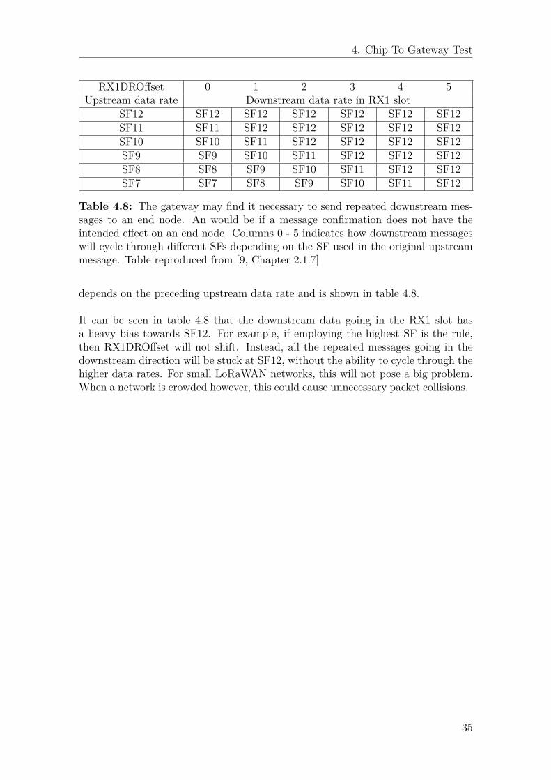
4. Chip To Gateway Test
RX1DROffset 0 1 2 3 4 5Upstream data rate Downstream data rate in RX1 slot
SF12 SF12 SF12 SF12 SF12 SF12 SF12SF11 SF11 SF12 SF12 SF12 SF12 SF12SF10 SF10 SF11 SF12 SF12 SF12 SF12SF9 SF9 SF10 SF11 SF12 SF12 SF12SF8 SF8 SF9 SF10 SF11 SF12 SF12SF7 SF7 SF8 SF9 SF10 SF11 SF12
Table 4.8: The gateway may find it necessary to send repeated downstream mes-sages to an end node. An would be if a message confirmation does not have theintended effect on an end node. Columns 0 - 5 indicates how downstream messageswill cycle through different SFs depending on the SF used in the original upstreammessage. Table reproduced from [9, Chapter 2.1.7]
depends on the preceding upstream data rate and is shown in table 4.8.
It can be seen in table 4.8 that the downstream data going in the RX1 slot hasa heavy bias towards SF12. For example, if employing the highest SF is the rule,then RX1DROffset will not shift. Instead, all the repeated messages going in thedownstream direction will be stuck at SF12, without the ability to cycle through thehigher data rates. For small LoRaWAN networks, this will not pose a big problem.When a network is crowded however, this could cause unnecessary packet collisions.
35

4. Chip To Gateway Test
36

5Network design
The design of a specification for intermediate-nodes is discussed and presented in thischapter. The use case for intermediate nodes is to reliably extend the network rangewithout having to add additional, expensive gateways. A successful specification ofintermediate nodes would allow for reliable transmission over at least a double-hoplink, making the installation of weather stations feasible in more locations.
5.1 ConsiderationsWhen designing the protocol for the intermediate nodes the weather station usecase along with the limitations of the LoRa protocol have to be considered. In thissection some several of the, what we consider, most important considerations whendesigning a range extending network specification are listed and shortly discussed.
5.1.1 Range of LoRaAs stated in LoRaWAN marketing material nodes can have a range of up to 15 kmor further when in line of sight. However, the range of the LoRa protocol depends onmultiple factors, such as data rate, weather and line of sight. Given steady weatherconditions and data rate, the further a transmitter moves from a receiver, the higherthe PER will become. To combat the increasing PER the data rate can be lowered.Therefore, in this network specification, a trade-off between data rate and range hasto be made. The results of the chip to gateway test, presented in section 4.4, can beused to make an informed decision about a suitable data rate which balances boththe range and data rate criteria.
5.1.2 Frequency ChannelThe ETSI regulations and LoRa regional parameters specification [9] specify thatfrequencies between 863 MHz and 870 MHz can be used. Furthermore, the spec-ification requires each chip to implement at least three different channels, 868.10MHz, 868.30 MHz and 868.50 MHz. These channels are used to guarantee a min-imal common channel set between end-devices and gateways. However, for theintermediate-nodes, the possibility of deviating away from this common set of fre-quency channels exists and it might even be wise to do so in order to avoid collisions.One of the main considerations when deciding on which frequency channel to useis whether all units should communicate on the same channel, simplifying setup
37

5. Network design
and operation of the nodes, or whether each intermediate node should form its ownsmall cluster communicating on its own frequency channel. The advantages anddisadvantages of both methods are listed below.
Single frequencyThe main advantage of using a single frequency for communication betweenthe end-devices and intermediate nodes is that it simplifies setup and oper-ation of the nodes. A new end-device or intermediate-node can be insertedanywhere in the network and it can start communicating right away withoutany additional setup. Furthermore, if there are multiple intermediate nodes inrange of an end-device, all intermediate nodes will receive and have the abilityto forward the message, increasing redundancy and possibly minimizing theneed for re-transmissions by the end-device (if re-transmission is used). If oneintermediate-node goes down, some end-devices might still be able to reachother intermediate nodes and stay online. However, this simplicity and redun-dancy comes at a cost of an increased chance of collisions and lower networkthroughput. Assuming a simple Aloha protocol [25] is used for multiple access,the risk of collisions will grow with an increasing number of nodes, increasingthe risk of dropped frames.
Multiple frequencies / cellsCreating smaller cells around each intermediate-node, where each cell com-municates on its own frequency channel has some considerable advantages. Acell implementation where each cell utilizes a frequency channel that does notintersect with neighbouring cells removes the risk of inter-cell collisions. As-suming a simple Aloha protocol approach for multiple access, in-cell collisionsare still possible. However, if the cells are kept small the collision risk willbe minimal compared to a single frequency setup. The main drawback of afrequency cell setup is that it requires extra steps during setup/commissioningof the system. Furthermore, when adding additional end-devices each end-device must be configured to match its intended intermediate node. Whenadding a new intermediate-node a new cell needs to be created and the end-devices which connects to it need to be configured or re-configured to matchthe settings of the new intermediate-node. Another big drawback for the celllayout is that it has no redundancy built in if an intermediate-node goes down,meaning all end-devices connected to an intermediate node go down with it.
It is clear that both the single frequency and multiple frequencies approach havetheir advantages and disadvantages. Both approaches described above can be seenas extremes and a compromise might be a valid idea. A possible compromise wouldbe to limit the multiple frequencies method in a way, such that it would easier to addnew intermediate-nodes and additional end-devices without a cumbersome setup. Apossible approach is described below.
Mixed approachInstead of configuring each intermediate-node and all end-devices belonging
38

5. Network design
to the cell, we only configure the intermediate-node to respond to differentfrequencies. The end-devices are then configured, such that they contain a listof legal frequency channels. When a new end-device is added to the network ora cell, it transmits a join message, cycling through the frequency channel listuntil it receives a response. This way you get a simple setup but most of thebenefits of a multiple cell system. However, if an intermediate-node goes down,the system still does not have the redundancy of a single frequency system.Furthermore, this solution requires bi-directional communication while theother solutions only require an uplink connection from the end-devices to theintermediate node.
As can be seen from the methods above, no clear cut solution exists. The aforemen-tioned methods all have their advantages and drawbacks which have to be consideredwhen creating the network specification.
5.1.3 Spreading Factor
An additional limitation imposed by using an intermediate-node compared to agateway is that in general, the transceivers in the end-devices/intermediate-nodesonly support listening to a single channel and a single spreading factor at the sametime. This requires the intermediate-nodes and end-devices to agree on using asingle spreading factor for communication. Like multiple frequency channels canbe used to differentiate between network cells if a multiple- or mixed frequency ap-proach from section 5.1.2 is used, the spreading factor can be used to differentiatebetween different cells if a single frequency is shared by all cells. However, usingmultiple spreading factors has some obvious drawbacks compared to using multiplefrequencies to differentiate between cells. The main drawbacks are that there arefewer spreading factors available for use compared to frequency channels and thatspreading factors drastically affect the range and data rate of the network. The factthat the spreading factor dictates the range and data rate is also our main consider-ation when choosing which factor to use, so creating different cells by use of differentspreading factors might be counterproductive.Due to the effects that the spreading factor has on the data rate, it can severelyimpact the network usability. Accounting for LoRa’s duty cycle restrictions and lowdata rates, choosing a high spreading factor, which has a low data rate, will have anegative effect on transmission collisions. Furthermore, if a collision occurs for thesehigher spreading factors, the transmitter will have used up a fair bit of its duty cycleand might not be able to re-transmit its message due to duty cycle limitations. Forexample, according to LoRa Modem Calculator Tool a 16 byte message with a 10.25symbol preamble length has a time on air of 926 ms.
This limits a transmitter to a maximum of around 36 messages per hour, includingre-transmissions. This perhaps is no issue for a small network with few nodes, butcan become cumbersome when the network grows. Furthermore, the longer rangeof the higher spreading factors (SF10, SF11, SF12) compared to the lower spread-ing factors (SF7, SF8, SF9) increases the likelihood of collisions. Therefore a lower
39

5. Network design
spreading factor is preferred, as it allows for less interference between nodes, higherdata rates and reduces likelihood of collisions compared to higher spreading factors.
5.1.4 Message and Node IdentificationIn a regular LoRaWAN, a sender and a message can easily be identified by thenetwork due to the built in headers. However, when using intermediate nodes,this becomes less straight forward due to fact that no MAC-layer information issent when the devices utilize the LoRa protocol for point-to-point communicationbetween themselves outside of LoRaWAN. Thus, the intermediate node has to wrapthe message it is forwarding in its own header. Due to this wrapping, the messageappears to originate from the intermediate-node. Therefore it will be hard to tellwhere a message is originating from on a network level, instead extra logic hasto be added to the receiving application, such that it can distinguish the receivedmessages. In order to distinguish the messages, each sender and each message needsto include a unique identifier that an application can make use of. As the datarates supported by LoRa are very low and we have strict duty-cycle restrictions, themain consideration for identifiers is to keep them small. Due to the fact that theintermediate-nodes has to forward these identifiers, keeping them small could allowfor higher throughput and for more messages to be bundled together when they arebeing forwarded by the intermediate-node.
5.1.5 Acknowledgement of reception by intermediate nodeIdeally it would be good to have the intermediate node send an acknowledgementthat it has received a message by an end-device. This can be used to ensure that themessage reaches its destination as the end-device can re-transmit until it receives anacknowledgement from the intermediate node. If the network consists of radio cells,the use of acknowledgements might increase the networks ability to self-heal in caseof outage of an intermediate node. If an end-device does not receive an acknowl-edgement in a pre-determined time, it tries to join another cell. Acknowledgements,however, have some drawbacks too. One of the main drawbacks is that there is nobuilt-in acknowledgement message for the radio protocol, meaning that this func-tionality would have to be implemented in software. Furthermore, due to duty cyclelimitations the end-device may inadvertently use up its duty cycle allocation duringre-transmission or the intermediate-node might use up all its duty cycle for acknowl-edgements, leaving it unable to forward the received messages. This could lead tofurther loss of messages. As weather data is generally slow varying with time, itis not critical that each and every message reaches its destination. Therefore, itmight be wiser to simply increase the update frequency of the weather data insteadof using acknowledgements.
5.1.6 Transmission protocolOne of the simplest transmission protocols is known as Aloha [25]. In Aloha, eachend-device that has any data to transmit, transmits its data whenever it is ready
40

5. Network design
to do so. For our network, this simple approach is desirable. As the Aloha protocoldoes not require time synchronization, it becomes extremely easy to implement. Themain drawback of the Aloha protocol is that is has a max throughput of only 1/2e ≈0.18 = 18% [25]. However, due to the small number of nodes in our network andlow message frequency from each node, network congestion is not of huge concern.Another notable transmission protocol to consider would be Slotted Aloha, this isan improved version of Aloha, where end-devices are only allowed to transmit duringpredefined transmission slots. Slotted Aloha has double the maximum throughput ofthe simple Aloha protocol, which gives a maximum throughput of 1/e ≈ 0.36 = 36%.However, slotted aloha requires time synchronization between end-devices such thatall transmission slots align correctly. The time synchronization can however be veryhard to achieve and we therefore wish to avoid implementing it if possible. Thesimple Aloha protocol is thus considered to be best suited for our needs.
5.1.7 Data transmission frequency
The end-devices and intermediate-nodes in this network will be transmitting weatherdata to an end application. Although weather often seems to change from minute tominute, the weather is rather slow varying and we do not need such high granularitydata for the intended application. Each end-device might not necessarily need totransmit aggregated weather data more often than once every 5 or 10 minutes.This allows for long intervals where the radio is powered of and therefore also savesbattery, prolonging the lifetime of the node. We also see that even at high spreadingfactors, we will not be able to fully utilize the duty-cycle if our transmission frequencyis kept below a single message every 5 minutes. However, we have to considerthat if all nodes transmit their updates at an equal update frequency, this mightcreate continuing message collisions, resulting in lost data. This is due to the factthat if two devices experience a transmission collision, but neither device gets anyfeedback about the collision, they will keep transmitting messages with the samefrequency, continuing the message collisions in perpetuity. Therefore, introducingsome randomness to the update frequency of the weather data might be necessaryto avoid this scenario.
5.1.8 Packet size from intermediate-node to Gateway
Since the information the nodes transmits is of fixed length, there is no reason tohave variable packet lengths between end-devices and intermediate-nodes. However,the intermediate-nodes may have received several packets from end-devices beforethey re-connect to the LoRaWAN network for forwarding of the stored messages.Due to the short message format used to transmit the weather information, the MACheaders in the LoRaWAN protocol can be a significant part of the total transmittedmessage. It would therefore be beneficial to aggregate the data and transmit severalof the stored messages as a single message from the intermediate-node to the gateway.
41

5. Network design
5.1.9 SecurityThe PHY layer LoRa protocol does not offer any encryption options like the MAClayer LoRaWAN protocol does. The LoRa protocol only offers the option of a cyclic-redundancy-check, which checks the message integrity, but provides no encryption.Therefore, unless implemented by the end-devices and intermediate-nodes, all mes-sages between those two parties will be sent in the clear. Although the weatherdata itself perhaps is not very sensitive information that needs to be protected, thelack of encryption and lack of a secure way for end-devices to identify themselvesand intermediate-nodes to verify this identification means that the system is veryvulnerable. A possible vulnerability would be an injection attack where an attackerposes as an end-devices and transmits false data to the intermediate-node. Thiscould inject false values into the end application. In a long-term implementation ofthis kind of network, the security needs to be taken into account.
5.1.10 Over The Air UpdatesAs is known, engineers don’t always get things right on the first try and devicesneed to be maintained, the need to update the device software arises. Due to thespread out nature of the devices it would be beneficial to have the means of up-dating the end-devices and intermediate-nodes over the air (OTA). However, doingOTA updates requires bi-directional communication. As mentionend in chapter 2,LoRaWAN supports bi-directional communication, but it is very limited. Further-more, OTA updates of end-devices also requires bi-directional communication be-tween the intermediate-nodes and end-devices, adding additional complexity to theprotocol. On top of the communication limitations, OTA updates will require addi-tional means to verify that the received update is correct and initiated by a trustedparty. We therefore suggest that OTA updates should not be made available.
5.2 Network Extending SpecificationHaving listed and discussed considerations for a network extending specificationfor intermediate-nodes in the previous section, an implementable specification isproposed in this section. The specification is intended to be used in conjunction witha LoRaWAN as intermediate-nodes need to intermittently connect to a LoRaWANfor message forwarding to a centralized network server. The aim of this specificationis thus to define how end-devices and intermediate-nodes communicate.
5.2.1 Range of LoRa - Placement of nodesThe placement of a node depends on a large number of parameters. While eachlocation needs to be evaluated, there are a few guide lines worth mentioning here.The first thing to consider is the surroundings of the communications link. It isassumed that all nodes will be located at sufficient height to compensate for Earth’scurvature, in accordance with the quick guide given in chapter 3.3.1).
42

5. Network design
Distance 1 km 3 km 5 km 7 km 9 km
Fresnel zone 1maximum radii 9.3 m 16.1 m 20.8 m 24.6 m 27.9 m
Recommendedclearance 8.6 m 12.7 m 15.5 m 17.8 m 19.7 m
Table 5.1: Maximum Fresnel radii and the accompanying recommended clearancesfor possible transmitter-receiver distances in intermediate-node connections
Supposing then that the scenery will be similar to the archipelago outside of Gothen-burg, a large part of the environment will consist of water. Although calm watercan reflect a signal favorably from the perspective of a receiver, it is probably unwiseto assume open water to always behave. Even when relatively calm, highly reflec-tive surfaces can cause unwanted effects. These effects were mentioned in 4.4 whendiscussing the RSSI variations between measurements taken at transmitter-receiverdistance of five and seven kilometers. Although two kilometers further apart, theextra antenna-heights provided at the seven kilometer distance resulted in a sizableRSSI increase compared to the five kilometer distance.
Recalling the Fresnel zone clearance, mentioned in section 3.3.2), equation (3.15)can be used to calculate the first Fresnel zone radius for probable distances inintermediate-node communication links. The maximum radii can be seen in table5.1.Using the maximum heights as references, the recommended clearances, utilizingthe 60% plus an additional three meters rule, are given in table 5.1.
5.2.2 Frequency ChannelFor the intended application of weather stations, we propose to utilize a singlefrequency channel for communication between end-devices and intermediate-nodes.Preferably we would recommend the making use of a frequency channel between 868and 868.6 MHz or 869.7 and 870 MHz to as it allows for a duty cycle of 1% in com-pliance with ETSI regulations. The communication between the intermediate-nodesand the gateway would be relegated to the pre-defined default frequency channelsof 868.1 MHz, 868.3 MHz and 868.5 MHz. Therefore, in order to minimize the colli-sion risk, the upper frequency band of 869.7 to 870 MHz might be better suited forend-device to intermediate-node communication. As the weather station networkis relatively sparse, the benefits of a simple single frequency network outweigh thedrawbacks. Furthermore, due to the sparse nature of the weather stations, it isunlikely that they will run into network congestion problems.
5.2.3 Spreading FactorIn order to decrease the time on air for the end-devices we wish to keep the spread-ing factor as low as possible. Our testing showed that with good placement of the
43

5. Network design
gateway and end-devices, such that line of sight was achievable, there was very littledifference in PER between SF7, SF8 and SF9 even as distances grew to 7 km. How-ever, these tests represent a best case scenario where we have a gateway with a highergain antenna and possibly a more sensitive receiver compared to an RN2483 chip.Therefore we might experience a performance drop when going from end-device togateway to end-device to intermediate-node, which both utilize the same RN2483chip. With well placed intermediate-nodes and end-devices this should not have aconsiderable negative effect of the performance. We therefore suggest utilizing SF8for communication between end-devices and intermediate-nodes. As the data theweather stations are transmitting is fixed and of a limited nature, SF8 should easilyprovide the necessary data rate and range, while minimizing time on air for theend-devices. Another benefit of choosing a low spreading factor is that it allowsfor either an increased update frequency of weather data or increased number ofend-devices.
For the communication between an intermediate-node and a gateway we suggestusing SF7 for data transmission. In our testing we saw that the performance of SF7with regards to PER was stable even with increasing range. In addition, for thisproject the gateway would be placed on a mast on top of SSRS office in Långedrag.With smart placement of the intermediate-nodes this allows for line of sight com-munication between the intermediate-nodes and gateway, mirroring the environmentof our testing and as such we can expect similar performance. Another reason forrecommending SF7 or a lower spreading factor than the end-devices use, is that theintermediate-node must be able to aggregate and transmit all the data received fromthe end-devices, within its own duty cycle. Of course, if there are few end-devicesor/and the update frequency of the weather data is limited, the intermediate-nodewill be able to aggregate and transmit the received data even if using the sameor possibly a lower spreading factor. However, choosing a lower spreading factor,allows for either more devices in the network or a higher update frequency, whichboth are desirable traits.
5.2.4 Message and Node IdentificationEach node should be given a unique two byte node identification number duringcommissioning, this number is then always included when the node transmits aframe of data. This allows for 65536 unique nodes in the network. For messageidentification, a two byte number is included in and incremented with each trans-mitted frame. When the frame counter reaches 65535 it is reset to 0 and resumesordinary operation.
5.2.5 Acknowledgement of reception by intermediate nodeThere will be no acknowledgement procedure implemented in this network protocol.The main reason for this is simplicity, battery-life and duty cycle limitations. Inaddition, the data to be transmitted by the end-devices is weather data, which isusually slow varying, meaning the end application does not suffer from intermittent
44

5. Network design
Node ID Frame Counter Payload CRC2 Bytes 2 Bytes 10 Bytes 2 Bytes
Figure 5.1: Message format
loss of messages. Instead of using acknowledgements, it is suggested to increasethe update frequency of weather data such that a higher transmission loss can betolerated. Although, it should be noted that increasing the update frequency canhave a significant negative effect on battery-life.
5.2.6 Transmission protocol and Data transmission frequencyThe network will utilize the Aloha protocol, due to its simplicity and ease of im-plementation. Thus, when a device has any data that it wishes to transmit, ittransmits it. However, update rate of data, also referred to as the data transmissionfrequency, must be taken into account here. In order to avoid continued collisionsbetween end-device transmissions, some randomness should be introduced into theupdate frequency of the data. The data transmission frequency is to be set at 300 swith a random factor of ±10%. If deemed necessary, this data transmission fre-quency can be updated to better suit the requirements of the network. That is, itcan be increased if the focus is more on battery-life and less on data granularity ordecreased (within duty cycle limitations) if data granularity is more important thanbattery-life.
5.2.6.1 End-device to intermediate-node
The packet size between end-devices and intermediate-nodes will be limited to 16-bytes. The first two bytes are a unique node identifier and the third and fourthbytes combine as a frame counter. The trailing 12-bytes are used for the weatherdata/payload and a cyclic redundancy check. The resulting message format can befound in figure 5.1.
The implementation of each field in table 5.1 is expanded on below.
Node ID:The node id is a unique identifier which should be set independently for eachnode. As the field is two bytes long, valid ID’s are between 0 and 65535. Thenetwork is therefore limited to 65535 unique devices.
Frame Counter:The frame counter is used to identify messages from end-devices. The framecounter is increased with each transmitted message until it reaches its upperlimit of 65535. When the frame counter is at its upper limit it starts againat 0. In addition to providing identification for messages the frame counterprovides a way to calculate PER.
45

5. Network design
Temp. Rain Pressure Wind Speed Humidity Wind Dir. CRC2 Bytes 2 Bytes 2 Bytes 2 Bytes 1 Byte 1 Byte 2 Bytes
Figure 5.2: Payload format
Byte Encoding5 MSB of measured temperature6 LSB of measured temperature7 MSB of measured rain8 LSB of measured rain9 MSB of measured air pressure10 LSB of measured air pressure11 MSB of wind speed12 LSB of wind speed13 MSB of measured humidity14 MSB of wind direction15 MSB CRC16 LSB CRC
Table 5.2: Byte order of payload
Payload:The payload format is designed to carry the sensor values from 6 sensors. Fig-ure 5.2 details the payload format and which data is collected and transmitted.To fit into this payload format, the data shall be encoded as seen in table 5.2.As the hardware design of the weather station is not yet complete, we can notmake final recommendations on how the data bytes should be used to representthe data. However, we will give general recommendations based on a formatused for the LoRaMOTE, which is a multi-purpose test device with similardata recording capabilities. The LoRaMOTE uses the MPL3115A2 chip [26],we therefore base our recommendations on the data format used by that chipas it is described in the LoRaMOTE users guide [23].Byte 5 and 6 represent a signed value of the measured temperature (x100)by the MPL3115A2 chip. The value can then be divided by 100 to get thetemperature with decimal values.Byte 7 and 8 represent the measured rainfall as an unsigned value. For therainfall we have no reference sensor, therefore we leave it up to implementationto decide how these two bytes should represent the value.Byte 9 and 10 represent the measured atmospheric pressure in deci-Pascal(dPa) as measured by the MPL3115A2 sensor. The number is therefore di-vided by 10 to get the hekto-Pascal number (hPa).Byte 11 and 12 are used to represent the measured wind speed. We have noreference sensor, but we suggest that the data should be measured and trans-mitted in mm/s.Byte 13 is used to represent humidity in percent. As this field is a single bytelong, it does not support decimal values, only whole numbers. If the chosen
46

5. Network design
sensor gives decimal values, they should be rounded to nearest integer.Byte 14 is used to represent wind direction. The wind direction as measuredby the sensor should be converted into an unsigned integer value between 0and 255. The measured degree value is converted into the integer by dividingthe measured value by 360/256 ≈ 1.40625. The integer value can then beconverted to a degree value by multiplying it by 360/256 ≈ 1.40625.Byte 15 and 16 are used for a cyclic redundancy check. See section 5.2.7 foradditional information.
5.2.6.2 Intermediate-node to Gateway
The payload format used between the intermediate-node and gateway is very sim-ilar to the format described in section 5.2.6.1. The only difference is that theintermediate-node has a variable payload length and can aggregate several receivedmessages into a single message for forwarding. Therefore, the intermediate-nodeframe format contains a single byte header which informs the application aboutthe number of forwarded messages the incoming message contains. That is, if theintermediate-node is forwarding three messages, it will set the first byte value to 3and then concatenate the 42 message bytes (3 x 14 Bytes) before transmission. Thisis illustrated in figure 5.3.
No. Messages Message 1 Message ... Message N1 Byte 14 Bytes 14 Bytes 14 Bytes
Figure 5.3: Intermediate-node frame format
This allows the intermediate-node to forward as many messages as it deems neces-sary, within the rules of the regional parameters as described in section 2.3.4.2.In addition to forwarding messages, the intermediate-nodes can themselves be end-devices/weather stations. Therefore, each intermediate node also contains its ownunique identifier and frame counter, as described earlier, and forwards its own mes-sages in the same way as it would with any message received from an end-device.
5.2.7 SecurityThere is no built in encryption in the LoRa physical layer protocol. However, westrongly recommend that some encryption is used for the payload. We suggestmaking use of symmetric encryption, where the end-devices and intermediate-nodesshare the same key. The key therefore has to be known by the intermediate-nodesand end-devices when they are being deployed. The reason for choosing symmetricencryption over asymmetric encryption, is that symmetric encryption usually re-quires shorter keys than asymmetric encryption. This makes the encryption easierto use on the very limited hardware that the weather stations will contain. Fur-thermore, as we have the option of distributing the keys during deployment, theadvantage of asymmetric encryption is little to none.We also wish to add a cyclic redundancy check to the end of the message, whichgives additional error detection capabilities. We assume that the hardware we use
47

5. Network design
will be based on Arduino, therefore we suggest making use of AES_128 encryption.This is the same encryption standard that is being used by LoRaWAN. Further-more, there already exists a good implementation called Arduino AESlib [27]. Thissimplifies usage considerably. For the cyclic redundancy check, there exists a goodArduino library called crc-16 [28]. The CRC should be calculated and added to theend of the payload before encryption. This both ensures that the CRC is immutableand furthermore creates a message of 16 bytes, which is the necessary input lengthfor the encryption functions in the AES_128 library. The encryption key used be-tween the end-devices and intermediate-nodes should differ from the Network- andApplication Keys used for the LoRaWAN setup. This is to ensure that even in theevent that the encryption key is leaked, devices will not be able to use it to connectto the LoRaWAN network. Furthermore, the AES_128 encryption key should berandomly generated, not chosen by the implementer.
5.2.8 Over The Air UpdatesNo mechanism for OTA updates shall be implemented. As OTA updates require bi-directional communication, the additional complexit and drawbacks of implementingit outweigh the advantages.
5.2.9 Connecting to and leaving LoRaWANThe intermediate nodes must regularly connect to the LoRaWAN to forward receiveddata and transmit collected data. When leaving the LoRaWAN, the RN2483 chipsissue a mac-pause command and get a response telling them the amount of millisec-onds they can leave the network for. The intermediate-nodes must therefore re-jointhe LoRaWAN before this time is exceeded. They should, however, limit their timeon the LoRaWAN as much as possible as their intermediate-node functionality isnone whilst they are connected to the LoRaWAN. Therefore, the intermediate-nodesshould only connect to the LoRaWAN when they have data to transmit or whenthey are about to exit the out-of-network time limit and then leave the LoRaWANagain as soon as possible.
48

6Discussion
6.1 LoRa and LoRaWANIn general the LoRa and LoRaWAN protocols seem well thought out and cater nicelyto the IoT use case. Having said that, both LoRa and LoRaWAN have some quirks.
6.1.1 LoRaThe LoRa modulation is a well suited for low-power and long-range, but suffersfrom a low data rate and low spectral efficiency. When used in the ISM bands,where duty cycles are strictly regulated, the use cases for LoRa are bound to nondata-heavy applications. Furthermore, the use of Hamming codes for FEC feelssomewhat counterproductive as the coding rate can be set to both 4/5 and 4/6,which introduces a 25-50 % increase in packet length, without introducing any errorcorrection capabilities.
From the tests performed in this project, it was concluded that LoRa modulationcan uphold low PER over the intended distances of the weather stations application.In order for the PER to stay sufficiently low however, the location of the transmittershad to be carefully planned. For long-distance end-nodes and intermediate-nodes inparticular, appropriate clearance had to be meticulously considered. Such require-ments make the deployment of LoRa capable nodes a more time consuming measurethan it might appear at first glance, epsecially for projects similar to this in scope.
6.1.2 LoRaWANThe LoRaWAN specification feels suitable for smaller deployments, where a networkoperator has control over most of the end-devices in the network. However, selling orgiving unrestricted access to a network to multiple different users can have cripplingeffects on the network. Assuming every user wishes to fully utilize the duty cycles itsdevices, the Aloha protocol quickly breaks down due to network usage. Furthermore,the LoRaWAN specification allows end-devices to send confirmed packets, meaningpackets should be acknowledged upon reception by a gateway. As the gatewaytoo is bound by the same duty cycle regulations imposed by ETSI in the ISMbands, the gateway’s duty cycle can be fully consumed by these acknowledgements.This leaves the gateway unable to respond to new incoming messages that requiresacknowledgement, creating additional network congestion as devices will re-transmitalready received messages due to the missing confirmation packets from the gateway.
49
6. Discussion
Therefore, a more complex protocol than Aloha or stricter duty cycle limitationsmight be required in the future as LoRaWANs grow bigger.
6.2 Network extension specification vs. additionalgateways
The network extension specification detailed in section 5.2 arises from the wish ofminimizing the number of gateways necessary in a network. Here, the advantagesand limitations of this approach are discussed. Suggestions are also made abouthow the proposed specification might be altered to better suit larger network de-ployments.
6.2.1 AdvantagesThe suggested network specification for extending networks with intermediate nodeshas some clear advantages compared to extending the network with additional gate-ways. They are listed below:
Low cost hardware and easy setup.The intermediate-nodes can be produced cheaply and their setup to the Lo-RaWAN is straightforward, just like any other LoRaWAN device. Comparedto an intermediate-node, an additional gateway is several times more expen-sive, both in hardware and running costs. The monthly subscription costs ofa gateway, for back-end and back-bone services, can easily surpass the cost ofan intermediate-node.
Homogeneous hardware.The specification is lightweight and is designed such that it can be easilyimplemented on the same hardware as the end-devices. Therefore, the onlydifference between a intermediate-node and an end-device is whether the de-vice contains software for acting as an intermediate-node or not. This makesit easy to re-purpose end-devices into intermediate-nodes or vice-verse if nec-essary. The main suggested hardware addition for intermediate-nodes is alarger battery in order to accommodate the increased energy consumption dueto the always listening nature and increased transmission rate, compared toend-devices.
No additional backbone connection necessary.Unlike a gateway, an intermediate-node does not require any additional back-bone connections, as itself is a relay node towards the gateway that has asteady backbone connection. The gateway’s backbone connection can eitherbe directly to the Internet through an Ethernet cable with network access orthrough a 3G network. These backbone connections can either be hard to findor costly to implement at the desired placement of an gateway making the
50

6. Discussion
intermediate-node a better choice.
Increased battery-life.As the intermediate-nodes contain far simpler hardware and only listens toa single frequency and SF, they draw less power than a gateway. This is animportant consideration as the intermediate-nodes are likely to be located inhard to reach locations, with limited power sources.
Friendlier to the environment.As the intermediate nodes consists of less hardware, they consume less re-sources and create less waste than a gateway. In addition, as mentioned above,during operation they consume less power than a gateway.
6.2.2 LimitationsA network utilizing the network extending specification, which uses intermediate-nodes, has several drawbacks and limitations compared to a network only utilizinggateways.
Single frequency and spreading factorCommunication between intermediate-nodes and end-devices are bound to asingle frequency channel and a single spreading factor. Meanwhile, the gate-ways can listen to multiple frequency channels and spreading factors simulta-neously. Therefore, the gateways introduce much more agility to the network.This also allows more end-devices to connect to each gateway compared tointermediate-nodes.
Simple hardwareThe intermediate-nodes contains far simpler hardware than the gateways.Therefore, using intermediate nodes instead of gateways can lower the avail-able link budget drastically, raising PER or limiting transmission range andplacement of end-devices.
One-way communication vs. Bi-directional communicationThe gateways offer bi-directional communication compared to the one-waycommunication of the intermediate-nodes. Although the bi-directional com-munication between gateways and end-devices is limited, it can be very useful.For example the bi-directional communication allows for adaptive data ratesand over-the-air activation (OTAA) of new nodes.
Low capacity of intermediate-nodesDue to the single frequency and single frequency setup of the intermediate-nodes, the network capacity is quicker to reach its limits compared to themulti-channel and multi-SF gateways.
51

6. Discussion
No OTAA capabilityThe intermediate-nodes do not have the ability of conducting OTAA for end-devices. Therefore, all new additions to the network have to be pre-configuredfor the network. Possibly slowing down roll-out of new devices. However, thisis perhaps not of great concern for a small network, such as the weather stationnetwork the protocol is designed for.
Lower data rate and fixed payload lengthDue to the fact that the intermediate-nodes implement a double-hop network,compared to the single-hop network that the gateway connections provide,the total throughput from end-device to gateway will be significantly lowerthan from an end-device to gateway. Furthermore, as the intermediate-nodehas to forward all its received data within its duty cycle limitations, it cre-ates even stricter duty cycle requirements for the end-devices that connect toit. The effective duty cycle of each end-device in a network of N end-devicesand an intermediate node becomes 1/(N + 1), assuming both intermediate-nodes and end-devices use the same spreading factor and that the end-devicesfully utilize their packets. However, as the packets that the end-devices trans-mit are limited to 14 bytes of information, the effective duty cycle can beslightly improved by aggregating the data in the intermediate node and thenforwarding it. This allows several end-device frames to share the overheadof a single intermediate to gateway message. If the communication betweenintermediate-node and gateway utilizes a higher data rate than the end-deviceand intermediate-nodes do, the effective duty cycle is less affected. However,utilizing only gateways, all end-devices can make full use of its duty cycle.
Back-end application logic necessaryUsing the intermediate-nodes requires an additional processing step to decodethe incoming message and attribute the data to the correct node. Utilizinggateways, the data can only originate from a single end-device. Therefore, ina gateway scenario, it is possible to make use of the device id that accompa-nies each LoRaWAN message instead of having to create new unique deviceidentifiers.
Lowered battery life of devices.Intermediate-nodes will have a significantly lower battery life than the end-devices. Compared to end-devices, the always listening nature of the intermediate-nodes, along with the message forwarding requirements which increases theirtransmission rates lowers the intermediate-nodes battery-life considerably. How-ever, compared to a gateway the intermediate-nodes will still consume lesspower. Though, in general, the gateways would be connected to a fixed power-source, lowering the importance of energy consumption considerations.
No adaptive data rate.Unlike the gateways, the intermediate-nodes offer no adaptive data rate. Thisnecessitates additional compromises on range and data rate between intermediate-
52

6. Discussion
nodes and end-devices as they must all use the same spreading factor. There-fore, end-devices located close to the intermediate node cannot utilize its loca-tion advantage compared to an end-device located further away, limiting thedata rate from end-devices to intermediate-nodes to the lowest commonly us-able data rate. Furthermore, forcing devices to use a higher SF than necessarylowers the battery life of the device as the higher SF requires longer transmittime.
6.2.3 Suggested network extension specification changes forlarger networks
The network specification detailed in chapter 5.2 is well suited for smaller, less densenetworks where the end-device count is low enough that we never reach the limits ofthe Aloha protocol. However, for larger and denser networks this network specifica-tion might break down due to some of the limitations mentioned above. Thereforefor larger deployments where the risk of running into the limits of the Aloha protocolis significant, some modifications to the protocol are therefore proposed. Perhapsthe first thing that should be re-visited is the payload format. The format works wellfor the intended weather station application but might not be optimal for other use-cases. It is still suggested that the payload format is kept to a fixed length multipleof 16, such that AES_128 encryption can be utilized. Furthermore, the continueduse of a CRC is encouraged. If a network is reaching the capacity limitations ofthe Aloha protocol, it is suggested the specification should introduce multiple fre-quencies and possibly multiple SF. This allows the network operator to set up cells,allowing for co-existence of cells due to frequency multiplexing, significantly improv-ing network capacity.
For a larger network implementation all these changes might be considered worth-while. However, for the relatively small network that the weather stations willcompose, these changes add unnecessary complexity. Another considerations is thatfor larger networks with dense end-device deployments the benefits of extending thenetwork with intermediate-nodes becomes less as each additional gateway that isdeployed will be able to serve a significant number of nodes. For these conditions,the advantages of a gateway might outweigh the advantages of the intermediate-node approach. Therefore, we believe that the network extensions specification isbest suited for small extensions to a LoRaWAN, with use cases such as the weatherstations or similar low density networks.
53

6. Discussion
54

7Conclusion
In this report the LoRa modulation and protocol, along with the LoRaWAN spec-ification has been explored. We found the LoRa and LoRaWAN protocols to becompetent and useful for IoT applications such as an IoT weather station network.
The FEC used in LoRa is found to be somewhat lacking as it offers four codingrates, where two rates don’t offer any error correction capabilities and one rate onlyintroduces an extra coding bit, but no additional error correction capabilities. Dis-regarding the FEC of the protocol, the LoRa modulation itself is sound, with linearfrequency modulation being a tried and tested approach to spread spectrum.
In our testing we found that LoRa and LoRaWAN both perform well with lowPERs at distances of up to 7 km when transmitting with line of sight. However,although the higher SF theoretically should outperform the lower SF, this was notthe case during our testing. A probable reason is that for the distances tested, themeasured RSSI values stayed within the sensitivity thresholds provided by each SF.
Another reason for the lack of performance differentiation between various SF mightbe due to the way that gateways in a LoRaWAN chooses which SF is used whenresponding to end-devices. Although our testings was performed with unconfirmedpackets such that the gateway should not transmit acknowledgement responses toeach received packet, the gateway still responded to one out of approximately 20packets. Due to us performing the testing with multiple different transmitters trans-mitting on different SF simultaneously and with regular intervals, the gateway sentresponses to several end-devices within a short time frame. As seen in Table 4.8,the gateway response messages are biased towards the higher SF. This bias to-wards the higher SF in conjunction with only three channels being used for up- anddownlink transmission, long transmission time of SF12 messages and multiple wellsynced transmitters used for testing creates a higher collision risk between up-linkmessages transmitted from end-devices with high SF and response messages sentfrom the gateway, compared to up-link messages sent on lower SF. When a collisionoccurs, we are likely to experience a packet error, leading to an undue increase inpacket errors on higher SF compared to lower SF. It should be noted that in normaloperation, where end-devices are not as well synced and can not utilize the networkas well as in our tests, the response messages from the gateways are less likely toaffect the PER as substantially. It is more likely that the LoRawWANs transmis-sion protocol would lead to high packet losses before the response routine of theLoRaWAN specification becomes highly disruptive.
55

7. Conclusion
We have discussed and specified a network extending protocol for LoRaWANs. Thenetwork extending protocol offers the possibility of extending a LoRaWAN in acheap and simple manner. The specification is found to be well suited for deploy-ment of smaller networks, where the extension only needs to handle a relativelysmall amount of units. When deploying larger networks the duty cycle limitationsand Aloha medium access protocol become prohibitive. For the use case of simpleIoT weather stations, the network extending specification is considered successful,although rather case-specific.
56
8Future work
This report has investigated LoRa and LoRaWAN, and explored how the combina-tion of modulation technique and network protocol might be useful for a weatherstation application. A specification that would allow for the weather stations to beplaced outside of the range of the gateway has been designed. However, the designspecifications have not yet been implemented. Thus, if permitted continued workon this project, implementation would be the logical next step. This would allowfor the design to be verified. In addition, it means that performance testing couldbe carried out as well as exploring how the protocol behaves in the real world. Itwould also be interesting to see how the protocols/networks throughput is affectedfor different data rates and for larger deployments. Furthermore, implementing bi-directional communication into the extension would make new use cases possibleand should also be worth exploring.
In addition to the weather data, future revisions of the weather stations might wishto transmit static images or even a live stream of current weather conditions. SinceLoRa is a low data-rate protocol, future upgrades to the weather stations mightneed to make use of some other protocol if they wish to fulfill those transmissionrequirements. Therefore it might be beneficial to look into other IoT-protocols op-erating in the ISM bands which might be able to offer higher data-rates. Of course,this would come at the cost of range and/or battery-life.
While the tests performed in this report has shown that low PER can indeed bemaintained over comparatively long distances, the performance is conditioned onclear LOS and adequately positioned transmitters. Another prerequisite that needsto be fulfilled is that the network must not run the risk of becoming congested. Forthe intended weather station application of this project, these requirements shouldbe realizable. However, should the employment of LoRaWAN networks see contin-ued increase, then the risk of interference from neighboring LoRa nodes will alsorise. Thus, an interesting subject for future development of this project is that ofinterference mitigation. A paper that has looked at said topic is [29]. The pa-per found that for networks experiencing varying levels of congestion, three closelyspaced gateways considerably improved the PER compared to employing a singlegateway, even if highly directional antennas were utilized. For future developmentof this project, further monitoring the findings of [29] could prove beneficial.
Lastly, one subject probably worth further investigating is what kind of applica-tions that LoRa and LoRaWAN are truly suited for. A study performed in the
57

8. Future work
paper [30] confirms the main drawback of LoRaWAN that has been already notedin this paper. That is, due to its restrictive duty cycles and low data rates, Lo-RaWAN is not a solution that caters all connectivity needs in the LPWAN space.Instead, every setup must be carefully designed to meet the requirements of eachuse case. Thus, a future development of this project could be to try and specifyapplications wherein LoRaWAN would have a high probability of performing well.
58

Bibliography
[1] P. Weyde. (May 31, 2017). Antalet sjöräddningsinsatser ökar - P4 Göteborg| Sveriges Radio, [Online]. Available: http : / / sverigesradio . se / sida /artikel.aspx?programid=104&artikel=6707458 (visited on 06/11/2017).
[2] ——, (Apr. 2, 2016). Kraftig ökning av sjöräddningsinsatser - Nyheter (Ekot)| Sveriges Radio, [Online]. Available: http : / / sverigesradio . se / sida /artikel.aspx?programid=83&artikel=6392915 (visited on 06/11/2017).
[3] LoRa Alliance. (Feb. 6, 2017). Lora-Alliance, [Online]. Available: https://www.lora-alliance.org (visited on 02/06/2017).
[4] Unkown. (Feb. 13, 2017). OSI model, [Online]. Available: en.wikipedia.org/wiki/OSI_model (visited on 02/13/2017).
[5] Semtech. (Mar. 15, 2017). AN1200.22 - LORA Modulation Basics, [Online].Available: www.semtech.com/images/datasheet/an1200.22.pdf (visited on03/15/2017).
[6] J. Pinkney, “Low Complexity Indoor Wireless Data Links Using Chirp SpreadSpectrum”, PhD thesis, Univerity of Calgary, 280 Discovery Place One, 3553-31 St. N.W., Calgary, Alberta, Dec. 2003, 243 pp.
[7] A. G. i Amat, SSY125 Digital Communications, Lecture Notes, Department ofSignals and Systems, Chalmers University of Technology, Nov. 2015, 121 pp.eprint: PDF.
[8] LoRa Alliance. (Feb. 6, 2017). Lora-Techonology, [Online]. Available: https://www.lora-alliance.org/What-Is-LoRa/Technology (visited on 02/06/2017).
[9] LoRa Alliance Technical committee, LoRaWAN - Regional Parameters, 1.0,LoRa Alliance, Inc., Jul. 2016, 45 pp.
[10] ETSI. (May 2012). ETSI EN 300 220-1 V2.4.1 (2012-05), [Online]. Available:www.etsi.org/deliver/etsi_en/300200_300299/30022001/02.04.01_60/en_30022001v020401p.pdf (visited on 05/18/2017).
[11] Semtech. (Jul. 2013). ETSI Compliance of the SX1272/3 LoRa Modem, [On-line]. Available: http : / / www . semtech . com / images / datasheet / etsi -compliance-sx1272-lora-modem.pdf (visited on 05/18/2017).
[12] ——, (Oct. 2013). Implementing Data Whitening and CRC Calculation inSoftware on SX12xx Devices, [Online]. Available: http://www.semtech.com/images/datasheet/AN1200.18_STD.pdf (visited on 06/01/2017).
[13] A. Oppenheim and A. Willsky, Signals & Systems, International Edition,2nd ed. Prentice-Hall International, 1997, 957 pp., isbn: 0-13-651175-9.
[14] A. Hein, Processing of SAR Data, Fundamentals, Signal Processing, Interfer-ometry. Springer Berlin Heidelberg, 2004, isbn: 9783662094570.
59

Bibliography
[15] Wikipedia. (Mar. 28, 2017). Horizon - Wikipedia, [Online]. Available: https://en.wikipedia.org/wiki/Horizon (visited on 05/20/2017).
[16] R. Freeman, Radio System Design for Telecommunications, 3rd ed. IEEE Press(John Wiley & Sons), 2007, 880 pp., isbn: 9780471757139.
[17] G. Orestis and R. Usman, “Low Power Wide Area Network Analysis: CanLoRa Scale?”, in IEEE Wireless Communications Letters, vol. 6, IEEE, 2017,pp. 162–165.
[18] J. Petäjäjärvi, K. Mikhaylov, A. Roivainen, T. Hanninen, and M. Pettissalo,“On the coverage of LPWANs: Range evaluation and channel attenuationmodel for LoRa technology”, in 2015 14th International Conference on ITSTelecommunications (ITST), IEEE, 2015, pp. 55–59.
[19] A. Goldsmith, Wireless Communications, 1st ed. Cambridge University Press,2005, 674 pp., isbn: 9780511841224.
[20] Semtech. (Jul. 2013). LoRa Modem Design Guide, [Online]. Available: http://www.semtech.com/images/datasheet/LoraDesignGuide_STD.pdf (visitedon 05/24/2017).
[21] F. Zandbergen. (Dec. 16, 2016). Kerlink LoRa IoT Station - Specifications -The Things Network, [Online]. Available: https://www.thethingsnetwork.org/docs/gateways/kerlink/specs.html (visited on 05/24/2017).
[22] Kerlink. (May 2017). WIRNET STATION 868 MHZ - Kerlink, [Online]. Avail-able: http : / / www . kerlink . fr / en / products / lora - iot - station - 2 /wirnet-station-868 (visited on 05/24/2017).
[23] Semtech. (Jul. 2014). LoRaMote - USER GUIDE, [Online]. Available: http://www.semtech.com/images/datasheet/User_Guide_LoRaMote_STD.pdf(visited on 05/23/2017).
[24] ——, (Mar. 2015). Semtech LoRa SX1272/73 - Datasheet, [Online]. Available:http://www.semtech.com/images/datasheet/sx1272.pdf (visited on05/28/2017).
[25] E. Modiano. (Apr. 25, 2017). Lecture 10/11: Packet Multiple Access: TheAloha protocol, [Online]. Available: http://web.mit.edu/modiano/www/6.263/lec10.pdf (visited on 04/25/2017).
[26] NXP B.V. (Sep. 13, 2016). MPL3115A2 datasheet, [Online]. Available: http://cache.freescale.com/files/sensors/doc/data_sheet/MPL3115A2.pdf(visited on 05/12/2017).
[27] D. Landman. (May 13, 2017). Arduino AESlib, [Online]. Available: https://github.com/DavyLandman/AESLib (visited on 05/13/2017).
[28] V. Mennella. (May 2017). Crc16 a simple crc-16 library for Arduino, [Online].Available: https://github.com/vinmenn/Crc16 (visited on 05/19/2017).
[29] T. Voigt, M. Bor, U. Roedig, and J. Alonso, “Mitigating Inter-network Interfer-ence in LoRa Networks”, in Proceedings of the 2017 International Conferenceon Embedded Wireless Systems and Networks, Arxiv.org - Cornell University,Feb. 20, 2017.
[30] F. Adelantado, X. Vilajosana, P. Tuset-Peiro, B. Martinez, J. Melia, and T.Watteyne, “Understanding the limits of LoRaWAN”, Jul. 2016.
60

AAppendix 1
−90 −85 −80 −75 −70RSSI [dB]
0
100
200
300
SF 7
AVG RSSI: -77.744 [dBm]
−85 −80 −75 −70 −65RSSI [dB]
0
50
100
150
200
SF 1
0
AVG RSSI: -74.392 [dBm]
−84 −82 −80 −78 −76 −74 −72 −70RSSI [dB]
0
100
200
300
400
SF 8
AVG RSSI: -74.554 [dBm]
−76 −74 −72 −70 −68 −66 −64RSSI [dB]
0
100
200
SF 1
1
AVG RSSI: -72.009 [dBm]
−110 −105 −100 −95 −90 −85 −80RSSI [dB]
0
50
100
150
200
SF 9
AVG RSSI: -96.339 [dBm]
−120 −110 −100 −90 −80 −70RSSI [dB]
0
50
100
150
SF 1
2
AVG RSSI: -95.468 [dBm]
Histogram of RSSI [dBm] for data collected at 1.0 km
Figure A.1: Histogram of RSSI for data collected at 1.0 km.
−94 −92 −90 −88 −86 −84 −82RSSI [dB]
0
100
200
300
SF 7
AVG RSSI: -86.533 [dBm]
−100.0 −97.5 −95.0 −92.5 −90.0 −87.5 −85.0 −82.5RSSI [dB]
0
50
100
150
SF 1
0
AVG RSSI: -92.891 [dBm]
−110 −105 −100 −95 −90 −85RSSI [dB]
0
50
100
150
200
SF 8
AVG RSSI: -97.662 [dBm]
−100.0 −97.5 −95.0 −92.5 −90.0 −87.5 −85.0 −82.5RSSI [dB]
0
50
100
150
SF 1
1
AVG RSSI: -92.542 [dBm]
−105 −100 −95 −90 −85RSSI [dB]
0
50
100
150
200
SF 9
AVG RSSI: -93.920 [dBm]
−120 −115 −110 −105 −100 −95 −90 −85 −80RSSI [dB]
0
50
100
150
SF 1
2
AVG RSSI: -91.726 [dBm]
Histogram of RSSI [dBm] for data collected at 3.0 km
Figure A.2: Histogram of RSSI for data collected at 3.0 km.
61

A. Appendix 1
−120.0 −117.5 −115.0 −112.5 −110.0 −107.5 −105.0 −102.5RSSI [dB]
0
50
100
150
SF 7
AVG RSSI: -116.173 [dBm]
−112 −110 −108 −106 −104 −102RSSI [dB]
0
100
200
300
SF 1
0
AVG RSSI: -107.196 [dBm]
−114 −112 −110 −108 −106RSSI [dB]
0
100
200
300
SF 8
AVG RSSI: -111.942 [dBm]
−120.0 −117.5 −115.0 −112.5 −110.0 −107.5 −105.0 −102.5RSSI [dB]
0
25
50
75
100
SF 1
1
AVG RSSI: -111.267 [dBm]
−117.5 −115.0 −112.5 −110.0 −107.5 −105.0 −102.5RSSI [dB]
0
100
200
300
SF 9
AVG RSSI: -111.815 [dBm]
−125.0 −122.5 −120.0 −117.5 −115.0 −112.5 −110.0 −107.5 −105.0RSSI [dB]
0
50
100
150
SF 1
2
AVG RSSI: -117.157 [dBm]
Histogram of RSSI [dBm] for data collected at 5.0 km
Figure A.3: Histogram of RSSI for data collected at 5.0 km.
−112.5 −110.0 −107.5 −105.0 −102.5 −100.0 −97.5 −95.0RSSI [dB]
0
100
200
SF 7
AVG RSSI: -104.626 [dBm]
−120 −115 −110 −105 −100RSSI [dB]
0
50
100
150
200
SF 1
0
AVG RSSI: -107.033 [dBm]
−120 −115 −110 −105 −100 −95RSSI [dB]
0
50
100
150
SF 8
AVG RSSI: -103.238 [dBm]
−120 −115 −110 −105 −100 −95RSSI [dB]
0
50
100
150
SF 1
1
AVG RSSI: -98.017 [dBm]
−120 −115 −110 −105 −100 −95RSSI [dB]
0
50
100
150
SF 9
AVG RSSI: -107.297 [dBm]
−125 −120 −115 −110 −105 −100 −95RSSI [dB]
0
25
50
75
100
SF 1
2
AVG RSSI: -106.547 [dBm]
Histogram of RSSI [dBm] for data collected at 7.0 km
Figure A.4: Histogram of RSSI for data collected at 7.0 km.
62

A. Appendix 1
0 200 400 600 800 1000Packet No.
−90
−85
−80
−75
−70
SF 7
, RSS
I [dB
] AVG RSSI: -77.744 [dBm]
0 200 400 600 800 1000Packet No.
−85
−80
−75
−70
−65
SF 1
0, R
SSI [
dB] AVG RSSI: -74.392 [dBm]
0 200 400 600 800 1000Packet No.
−85
−80
−75
−70
SF 8
, RSS
I [dB
] AVG RSSI: -74.554 [dBm]
0 200 400 600 800 1000Packet No.
−75
−70
−65
SF 1
1, R
SSI [
dB] AVG RSSI: -72.009 [dBm]
0 200 400 600 800 1000Packet No.
−110
−100
−90
−80
SF 9
, RSS
I [dB
] AVG RSSI: -96.339 [dBm]
0 200 400 600 800 1000Packet No.
−120
−100
−80
SF 1
2, R
SSI [
dB] AVG RSSI: -95.468 [dBm]
RSSI [dBm] for data collected at 1.0 km
Figure A.5: RSSI for data collected at 1.0 km.
0 200 400 600 800 1000Packet No.
−95
−90
−85
SF 7
, RSS
I [dB
] AVG RSSI: -86.533 [dBm]
0 200 400 600 800 1000Packet No.
−100
−95
−90
−85
SF 1
0, R
SSI [
dB] AVG RSSI: -92.891 [dBm]
0 200 400 600 800 1000Packet No.
−110
−100
−90
SF 8
, RSS
I [dB
] AVG RSSI: -97.662 [dBm]
0 200 400 600 800 1000Packet No.
−100
−95
−90
−85
−80
SF 1
1, R
SSI [
dB] AVG RSSI: -92.542 [dBm]
0 200 400 600 800 1000Packet No.
−105
−100
−95
−90
−85
SF 9
, RSS
I [dB
] AVG RSSI: -93.920 [dBm]
0 200 400 600 800 1000Packet No.
−120
−110
−100
−90
−80
SF 1
2, R
SSI [
dB] AVG RSSI: -91.726 [dBm]
RSSI [dBm] for data collected at 3.0 km
Figure A.6: RSSI for data collected at 3.0 km.
63
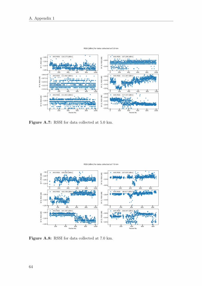
A. Appendix 1
0 200 400 600 800 1000Packet No.
−120
−115
−110
−105
SF 7
, RSS
I [dB
] AVG RSSI: -116.173 [dBm]
0 200 400 600 800 1000Packet No.
−110
−105
SF 1
0, R
SSI [
dB] AVG RSSI: -107.196 [dBm]
0 200 400 600 800 1000Packet No.
−115.0
−112.5
−110.0
−107.5
−105.0
SF 8
, RSS
I [dB
] AVG RSSI: -111.942 [dBm]
0 200 400 600 800 1000Packet No.
−120
−115
−110
−105
SF 1
1, R
SSI [
dB] AVG RSSI: -111.267 [dBm]
0 200 400 600 800 1000Packet No.
−115
−110
−105
SF 9
, RSS
I [dB
] AVG RSSI: -111.815 [dBm]
0 200 400 600 800 1000Packet No.
−125
−120
−115
−110
−105
SF 1
2, R
SSI [
dB] AVG RSSI: -117.157 [dBm]
RSSI [dBm] for data collected at 5.0 km
Figure A.7: RSSI for data collected at 5.0 km.
0 200 400 600 800 1000Packet No.
−110
−105
−100
−95
SF 7
, RSS
I [dB
] AVG RSSI: -104.626 [dBm]
0 200 400 600 800Packet No.
−120
−110
−100
SF 1
0, R
SSI [
dB] AVG RSSI: -107.033 [dBm]
0 200 400 600 800 1000Packet No.
−120
−110
−100
SF 8
, RSS
I [dB
] AVG RSSI: -103.238 [dBm]
0 200 400 600 800Packet No.
−120
−110
−100
SF 1
1, R
SSI [
dB] AVG RSSI: -98.017 [dBm]
200 400 600 800 1000Packet No.
−120
−110
−100
SF 9
, RSS
I [dB
] AVG RSSI: -107.297 [dBm]
0 200 400 600 800Packet No.
−120
−110
−100
SF 1
2, R
SSI [
dB] AVG RSSI: -106.547 [dBm]
RSSI [dBm] for data collected at 7.0 km
Figure A.8: RSSI for data collected at 7.0 km.
64

A. Appendix 1
−5.0 −2.5 0.0 2.5 5.0 7.5 10.0 12.5SNR [dB]
0
50
100
SF 7
AVG SNR: 8.861 [dB]
−5.0 −2.5 0.0 2.5 5.0 7.5 10.0 12.5SNR [dB]
0
50
100
SF 1
0
AVG SNR: 9.078 [dB]
2 4 6 8 10 12SNR [dB]
0
50
100
SF 8
AVG SNR: 9.830 [dB]
2 4 6 8 10SNR [dB]
0
50
100
150
200
SF 1
1
AVG SNR: 8.578 [dB]
−5 0 5 10SNR [dB]
0
50
100
150
SF 9
AVG SNR: 9.387 [dB]
−15 −10 −5 0 5 10SNR [dB]
0
100
200
SF 1
2
AVG SNR: 7.103 [dB]
Histogram of SNR [dB] for data collected at 1.0 km
Figure A.9: Histogram of SNR for data collected at 1.0 km.
2 4 6 8 10 12SNR [dB]
0
20
40
60
80
SF 7
AVG SNR: 8.808 [dB]
−5 0 5 10SNR [dB]
0
50
100
150
SF 1
0
AVG SNR: 8.421 [dB]
−10 −5 0 5 10SNR [dB]
0
50
100
SF 8
AVG SNR: 8.202 [dB]
−7.5 −5.0 −2.5 0.0 2.5 5.0 7.5 10.0SNR [dB]
0
50
100
150
200
SF 1
1
AVG SNR: 8.066 [dB]
−5.0 −2.5 0.0 2.5 5.0 7.5 10.0 12.5SNR [dB]
0
25
50
75
100
SF 9
AVG SNR: 10.120 [dB]
4 5 6 7 8 9 10 11SNR [dB]
0
25
50
75
100
SF 1
2
AVG SNR: 8.694 [dB]
Histogram of SNR [dB] for data collected at 3.0 km
Figure A.10: Histogram of SNR for data collected at 3.0 km.
65

A. Appendix 1
−8 −6 −4 −2 0 2 4 6SNR [dB]
0
20
40
60
SF 7
AVG SNR: -0.180 [dB]
−4 −2 0 2 4 6 8SNR [dB]
0
50
100
150
SF 1
0
AVG SNR: 5.944 [dB]
−6 −4 −2 0 2 4 6 8SNR [dB]
0
50
100
150
200
SF 8
AVG SNR: 5.489 [dB]
−15 −10 −5 0 5SNR [dB]
0
50
100
150
200
SF 1
1
AVG SNR: 3.302 [dB]
−4 −2 0 2 4 6 8 10SNR [dB]
0
50
100
150
SF 9
AVG SNR: 6.887 [dB]
−20 −15 −10 −5 0 5SNR [dB]
0
50
100
SF 1
2
AVG SNR: -3.254 [dB]
Histogram of SNR [dB] for data collected at 5.0 km
Figure A.11: Histogram of SNR for data collected at 5.0 km.
−10.0 −7.5 −5.0 −2.5 0.0 2.5 5.0 7.5 10.0SNR [dB]
0
50
100
SF 7
AVG SNR: 6.847 [dB]
−10 −5 0 5 10SNR [dB]
0
50
100
150
SF 1
0
AVG SNR: 6.590 [dB]
−5 0 5 10SNR [dB]
0
20
40
60
80
100
SF 8
AVG SNR: 7.946 [dB]
−10 −5 0 5 10SNR [dB]
0
50
100
SF 1
1
AVG SNR: 7.337 [dB]
−7.5 −5.0 −2.5 0.0 2.5 5.0 7.5 10.0 12.5SNR [dB]
0
20
40
60
80
SF 9
AVG SNR: 7.658 [dB]
−8 −6 −4 −2 0 2 4 6 8SNR [dB]
0
50
100
150
SF 1
2
AVG SNR: 5.681 [dB]
Histogram of SNR [dB] for data collected at 7.0 km
Figure A.12: Histogram of SNR for data collected at 7.0 km.
66
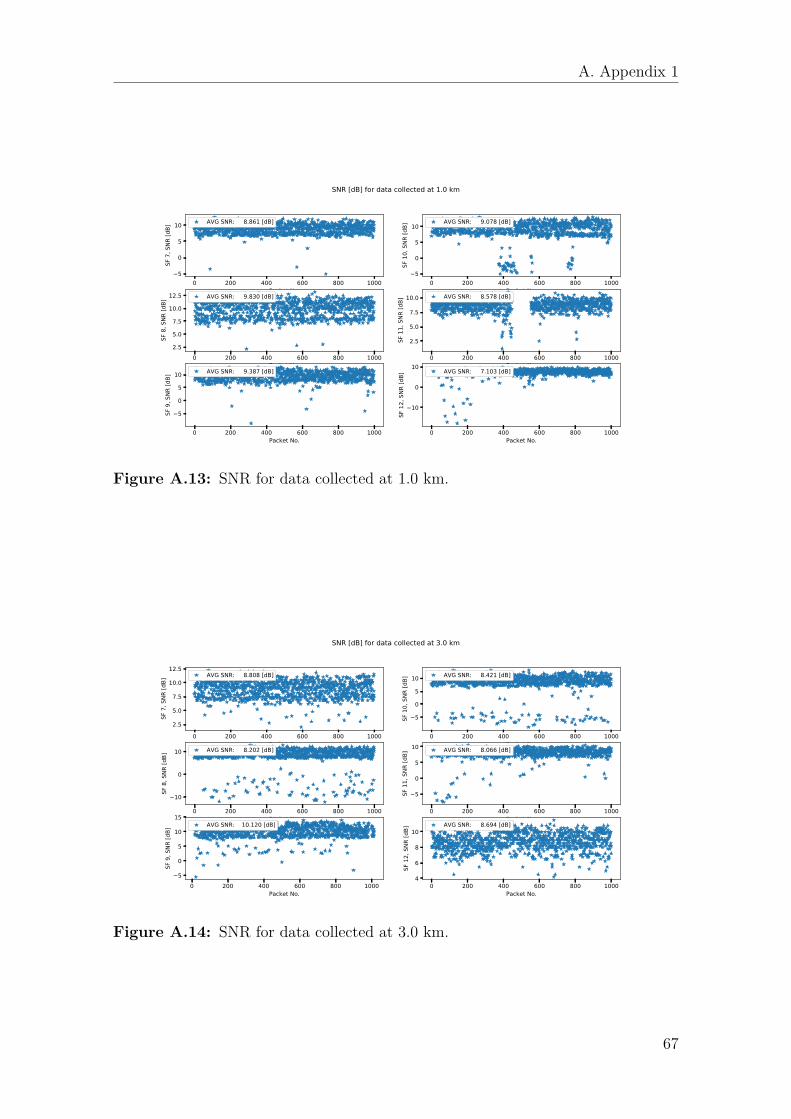
A. Appendix 1
0 200 400 600 800 1000Packet No.
−5
0
5
10
SF 7
, SNR
[dB]
AVG SNR: 8.861 [dB]
0 200 400 600 800 1000Packet No.
−5
0
5
10
SF 1
0, S
NR [d
B]
AVG SNR: 9.078 [dB]
0 200 400 600 800 1000Packet No.
2.5
5.0
7.5
10.0
12.5
SF 8
, SNR
[dB]
AVG SNR: 9.830 [dB]
0 200 400 600 800 1000Packet No.
2.5
5.0
7.5
10.0
SF 1
1, S
NR [d
B]
AVG SNR: 8.578 [dB]
0 200 400 600 800 1000Packet No.
−5
0
5
10
SF 9
, SNR
[dB]
AVG SNR: 9.387 [dB]
0 200 400 600 800 1000Packet No.
−10
0
10
SF 1
2, S
NR [d
B]
AVG SNR: 7.103 [dB]
SNR [dB] for data collected at 1.0 km
Figure A.13: SNR for data collected at 1.0 km.
0 200 400 600 800 1000Packet No.
2.5
5.0
7.5
10.0
12.5
SF 7
, SNR
[dB]
AVG SNR: 8.808 [dB]
0 200 400 600 800 1000Packet No.
−5
0
5
10
SF 1
0, S
NR [d
B]
AVG SNR: 8.421 [dB]
0 200 400 600 800 1000Packet No.
−10
0
10
SF 8
, SNR
[dB]
AVG SNR: 8.202 [dB]
0 200 400 600 800 1000Packet No.
−5
0
5
10
SF 1
1, S
NR [d
B]
AVG SNR: 8.066 [dB]
0 200 400 600 800 1000Packet No.
−5
0
5
10
15
SF 9
, SNR
[dB]
AVG SNR: 10.120 [dB]
0 200 400 600 800 1000Packet No.
4
6
8
10
SF 1
2, S
NR [d
B]
AVG SNR: 8.694 [dB]
SNR [dB] for data collected at 3.0 km
Figure A.14: SNR for data collected at 3.0 km.
67
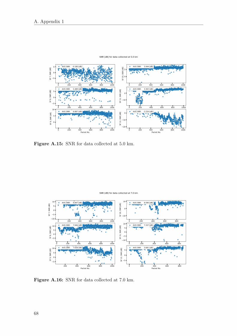
A. Appendix 1
0 200 400 600 800 1000Packet No.
−5
0
5
SF 7
, SNR
[dB]
AVG SNR: -0.180 [dB]
0 200 400 600 800 1000Packet No.
0
5
SF 1
0, S
NR [d
B]
AVG SNR: 5.944 [dB]
0 200 400 600 800 1000Packet No.
−5
0
5
SF 8
, SNR
[dB]
AVG SNR: 5.489 [dB]
0 200 400 600 800 1000Packet No.
−10
0
SF 1
1, S
NR [d
B]
AVG SNR: 3.302 [dB]
0 200 400 600 800 1000Packet No.
0
5
10
SF 9
, SNR
[dB]
AVG SNR: 6.887 [dB]
0 200 400 600 800 1000Packet No.
−20
−10
0
SF 1
2, S
NR [d
B]
AVG SNR: -3.254 [dB]
SNR [dB] for data collected at 5.0 km
Figure A.15: SNR for data collected at 5.0 km.
0 200 400 600 800 1000Packet No.
−10
−5
0
5
10
SF 7
, SNR
[dB]
AVG SNR: 6.847 [dB]
0 200 400 600 800Packet No.
−10
0
10
SF 1
0, S
NR [d
B]
AVG SNR: 6.590 [dB]
0 200 400 600 800 1000Packet No.
−5
0
5
10
SF 8
, SNR
[dB]
AVG SNR: 7.946 [dB]
0 200 400 600 800Packet No.
−10
−5
0
5
10
SF 1
1, S
NR [d
B]
AVG SNR: 7.337 [dB]
200 400 600 800 1000Packet No.
−5
0
5
10
SF 9
, SNR
[dB]
AVG SNR: 7.658 [dB]
0 200 400 600 800Packet No.
−5
0
5
SF 1
2, S
NR [d
B]
AVG SNR: 5.681 [dB]
SNR [dB] for data collected at 7.0 km
Figure A.16: SNR for data collected at 7.0 km.
68