exploring macroscopic quantum mechanics in optomechanical
TRANSCRIPT

Exploring Macroscopic QuantumMechanics in Optomechanical Devices
Haixing Miao
This thesis is in fulfillment of
Doctor of Philosophy
School of Physics
The University of Western Australia
2010

ii
Decrease your frequency by expanding your horizon.
Increase your Q by purifying your mind. Eventually,
you will achieve inner peace and view the internal
harmony of our world.
— A lesson from a harmonic oscillator
iii
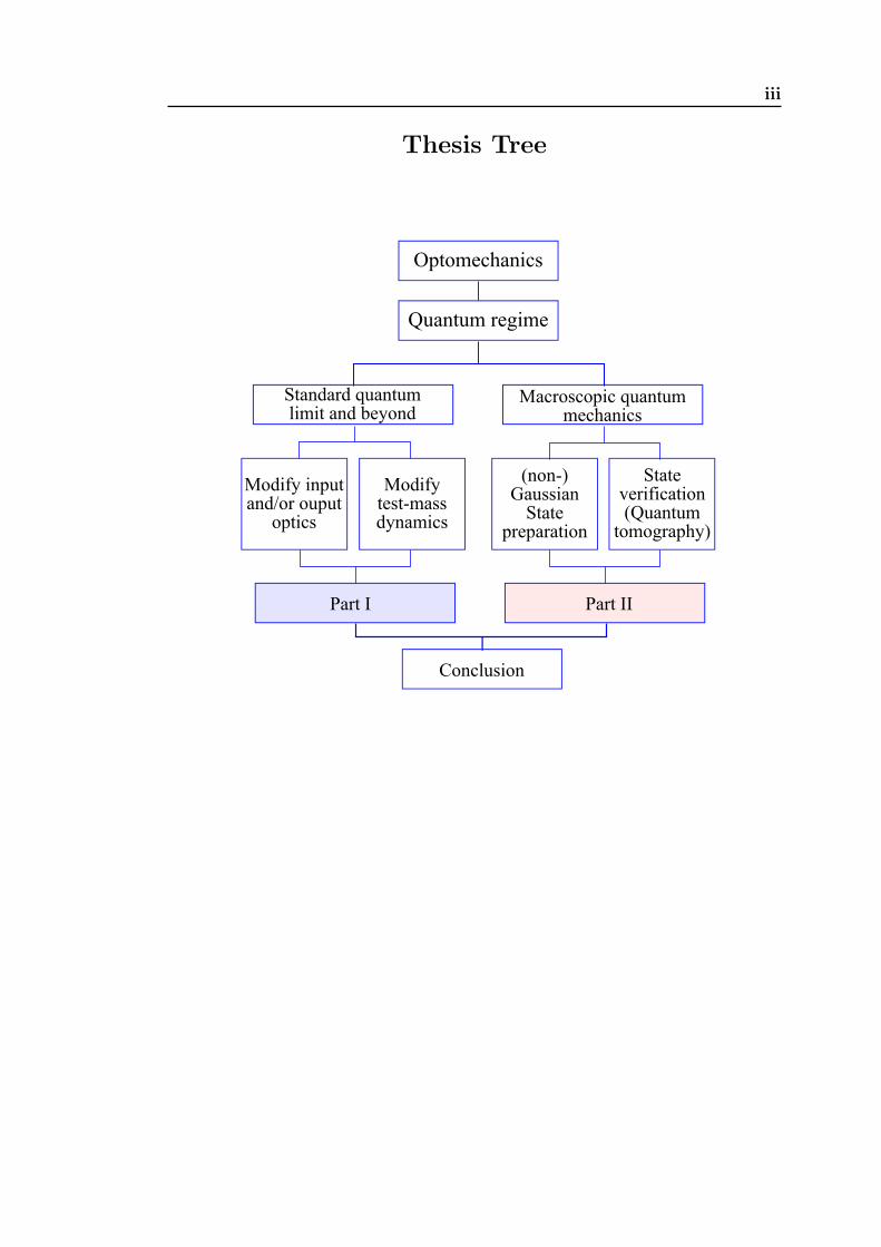
Thesis Tree
! !!
"


Acknowledgments
I am very thankful to my supervisors: Chunnong Zhao, David Blair and Ju Li atthe University of Western Australia (UWA), and Yanbei Chen at the CaliforniaInstitute of Technology (Caltech). With great patience and enthusiasm, they in-troduced me to many interesting topics, especially, optomechanical interactionsand their classical and quantum theories which make this thesis possible. When-ever I encountered some problems that could not be overcome, their sharp insightsand great motivations always lit me up, and helped me to move forward.
I also want to express my thankfulness to Stefan Danilishin, Mihai Bondarescu,Helge Muller-Ebhardt, Chao Li, Henning Rehbein, Thomas Corbitt, KentaroSomiya, Farid Khalili, and all the other members in the LIGO-MQM discus-sion groups. In the two months of visiting the Albert-Einstein Institute (AEI)and MQM telecons, I had intensive discussions with them, which produced manyfruitful results in this thesis. I thank especially Stefan who played significant rolesin all my work concerning macroscopic quantum mechanics.
I am very thankful to Rana Adhikari, Koji Arai, Kiwamu Izumi, Jenne Driggers,David Yeaton-Massey, Aiden Brook and Steve Vass at Caltech, with whom I spentmy enjoyable four-month experimental investigations of an advanced suspensionisolation scheme based upon magnetic levitation. Rana Adhikari and Koji Araimade painstaking efforts in trying to teach me the fundamentals of electronicsand feedback control theory.
I would like to thank Antoine Heidmann, Pierre-Francois Cohadon, and ChiaraMolinell for their friendly hosting of my visit to the Laboratoire Kastler Brossel,and for helping me to understand how to characterize a mechanical oscillatorexperimentally.
I thank all my colleagues at UWA: Yaohui Fan, Zhongyang Zhang, Andrew Sun-derland, and Andrew Woolley. They are easy-going and friendly, and the friend-ship with them has made my postgraduate study life colorful and enjoyable.
I would like to thank Ruby Chan for helping to arrange my visits to AEI andCaltech, and also for helping me with many other administrative issues.
I thank Andre Fletcher (UWA) for helping with proof-reading this thesis.
My research has been supported by the Australian Research Council and the

ii Chapter 0. Acknowledgments
Department of Education, Science and Training. Special thanks are due to theAlexander von Humboldt Foundation and the David and Barbara Groce startupfund at Caltech, which has supported my visit to AEI and Caltech.
Finally, I am greatly indebted to my beloved parents and my best friends: YiFeng, Zheng Cai, Shenniang Xu, Zhixiong Liang, Xingliang Zhu, and Jie Liu, whohave been supporting and encouraging me all the way along.

Abstract
Recent significant achievements in fabricating low-loss optical and mechanicalelements have aroused intensive interest in optomechanical devices which coupleoptical fields to mechanical oscillators, e.g., in laser interferometer gravitational-wave (GW) detectors. Not only can such devices be used as sensitive probesfor weak forces and tiny displacements, but they also lead to the possibilities ofinvestigating quantum behaviors of macroscopic mechanical oscillators, both ofwhich are the main topics of this thesis. They can shed light on improving thesensitivity of quantum-limited measurement, and on understanding the quantum-to-classical transition.
This thesis is a collection of publications that I worked on together with the UWAgroup and the LIGO Macroscopic Quantum Mechanics (MQM) discussion group.In the first part of this thesis, we will discuss different approaches for surpassingthe standard quantum limit for the displacement sensitivity of optomechanicaldevices, mostly in the context of GW detectors. They include: (i) Modifyingthe input optics. We consider filtering two frequency-independent squeezed lightbeams through a tuned resonant cavity to obtain an appropriate frequency depen-dence, which can be used to reduce the measurement noise of the GW detectorover the entire detection band; (ii) Modifying the output optics. We study atime-domain variational readout scheme which measures the conserved dynamicalquantity of a mechanical oscillator: the mechanical quadrature. This evades themeasurement-induced back action and achieves a sensitivity limited only by theshot noise. This scheme is useful for improving the sensitivity of signal-recycledGW detectors, provided the signal-recycling cavity is detuned, and the opticalspring effect is strong enough to shift the test-mass pendulum frequency from 1Hz up to the detection band around 100 Hz; (iii) Modifying the dynamics. Weexplore frequency dependence in double optical springs in order to cancel thepositive inertia of the test mass, which can significantly enhance the mechanicalresponse and allow us to surpass the SQL over a broad frequency band.
In the second part of this thesis, two essential procedures for an MQM experi-ment with optomechanical devices are considered: (i) state preparation, in whichwe prepare a mechanical oscillator in specific quantum states. We study the prepa-rations of both Gaussian and non-Gaussian quantum states, and also the creationof quantum entanglements between the mechanical oscillator and the optical field.Specifically, for the Gaussian quantum states, e.g., the quantum ground state, weconsider the use of passive cooling and optimal feedback control in cavity-assistedschemes. For non-Gaussian quantum states, we introduce the idea of coherently

iv Chapter 0. Abstract
transferring quantum states from the optical field to the mechanical oscillator. Forthe quantum entanglement, we consider the entanglement between the mechani-cal oscillator and the finite degrees-of-freedom cavity modes, and also the infinitedegrees-of-freedom continuum optical mode. (ii) state verification, in which weprobe and verify the prepared quantum states. A similar time-dependent ho-modyne detection method as discussed in the first part is implemented to evadethe back action, which allows us to achieve a verification accuracy that is belowthe Heisenberg limit. The experimental requirements and feasibilities of thesetwo procedures are considered in both small-scale cavity-assisted optomechanicaldevices, and in large-scale advanced GW detectors.

Contents
Acknowledgments i
Abstract iii
1 Introduction 1
2 Quantum Theory of Gravitational-Wave Detectors 13
2.1 Preface . . . . . . . . . . . . . . . . . . . . . . . . . . . . . . . . . 13
2.2 Introduction . . . . . . . . . . . . . . . . . . . . . . . . . . . . . . 13
2.3 An Order-of-Magnitude Estimate . . . . . . . . . . . . . . . . . . 14
2.4 Basics for Analyzing Quantum Noise . . . . . . . . . . . . . . . . 16
2.4.1 Quantization of the Optical Field and the Dynamics . . . . 16
2.4.2 Quantum States of the Optical Field . . . . . . . . . . . . 17
2.4.3 Dynamics of the Test-Mass . . . . . . . . . . . . . . . . . . 19
2.4.4 Homodyne detection . . . . . . . . . . . . . . . . . . . . . 20
2.5 Examples . . . . . . . . . . . . . . . . . . . . . . . . . . . . . . . 20
2.5.1 Example I: Free Space . . . . . . . . . . . . . . . . . . . . 21
2.5.2 Example II: A Tuned Fabry-Perot Cavity . . . . . . . . . . 23
2.5.3 Example III: A Detuned Fabry-Perot Cavity . . . . . . . . 24
2.6 Quantum Noise in an Advanced GW Detector . . . . . . . . . . . 26
2.6.1 Input-Output Relation of a Simple Michelson Interferometer 27
2.6.2 Interferometer with Power-Recycling Mirror and Arm Cavities 29
2.6.3 Interferometer with Signal-Recycling . . . . . . . . . . . . 31

vi Contents
2.7 Derivation of the SQL: a General Argument . . . . . . . . . . . . 34
2.8 Beating the SQL by Building Correlations . . . . . . . . . . . . . 36
2.8.1 Signal-recycling . . . . . . . . . . . . . . . . . . . . . . . . 36
2.8.2 Squeezed input . . . . . . . . . . . . . . . . . . . . . . . . 37
2.8.3 Variational Readout: Back-Action Evasion . . . . . . . . . 38
2.8.4 Optical losses . . . . . . . . . . . . . . . . . . . . . . . . . 39
2.9 Optical Spring: Modification of Test-Mass Dynamics . . . . . . . 40
2.9.1 Qualitative Understanding of Optical-Spring Effect . . . . 41
2.10 Continuous State Demolition: Another Viewpoint on the SQL . . 42
2.11 Speed Meters . . . . . . . . . . . . . . . . . . . . . . . . . . . . . 43
2.11.1 Realization I: Coupled cavities . . . . . . . . . . . . . . . . 44
2.11.2 Realization II: Zero-area Sagnac . . . . . . . . . . . . . . . 46
2.12 Conclusions . . . . . . . . . . . . . . . . . . . . . . . . . . . . . . 47
3 Modifying Input Optics: Double Squeezed-input 49
3.1 Preface . . . . . . . . . . . . . . . . . . . . . . . . . . . . . . . . . 49
3.2 Introduction . . . . . . . . . . . . . . . . . . . . . . . . . . . . . . 49
3.3 Quantum noise calculation . . . . . . . . . . . . . . . . . . . . . . 53
3.3.1 Filter cavity . . . . . . . . . . . . . . . . . . . . . . . . . . 53
3.3.2 Quantum noise of the interferometer . . . . . . . . . . . . 54
3.4 Numerical Optimizations . . . . . . . . . . . . . . . . . . . . . . . 56
3.5 Conclusions . . . . . . . . . . . . . . . . . . . . . . . . . . . . . . 60
4 Modifying Test-Mass Dynamics: Double Optical Spring 61
4.1 Preface . . . . . . . . . . . . . . . . . . . . . . . . . . . . . . . . . 61

Contents vii
4.2 Introduction . . . . . . . . . . . . . . . . . . . . . . . . . . . . . . 61
4.3 General considerations . . . . . . . . . . . . . . . . . . . . . . . . 63
4.4 Further Considerations: Removing the Friction Term . . . . . . . 65
4.5 “Speed-meter” type of response . . . . . . . . . . . . . . . . . . . 66
4.6 Conclusions and future work . . . . . . . . . . . . . . . . . . . . . 68
5 Measuring a Conserved Quantity: Variational Quadrature Read-out 69
5.1 Preface . . . . . . . . . . . . . . . . . . . . . . . . . . . . . . . . . 69
5.2 Introduction . . . . . . . . . . . . . . . . . . . . . . . . . . . . . . 69
5.3 Dynamics . . . . . . . . . . . . . . . . . . . . . . . . . . . . . . . 71
5.4 Variational quadrature readout . . . . . . . . . . . . . . . . . . . 72
5.5 Stroboscopic variational measurement . . . . . . . . . . . . . . . . 74
5.6 Conclusions . . . . . . . . . . . . . . . . . . . . . . . . . . . . . . 76
6 MQM with Three-Mode Optomechanical Interactions 77
6.1 Preface . . . . . . . . . . . . . . . . . . . . . . . . . . . . . . . . . 77
6.2 Introduction . . . . . . . . . . . . . . . . . . . . . . . . . . . . . . 78
6.3 Quantization of three-mode parametric interactions . . . . . . . . 80
6.4 Quantum limit for three-mode cooling . . . . . . . . . . . . . . . 83
6.5 Stationary tripartite optomechanical quantum entanglement . . . 87
6.6 Three-mode interactions with a coupled cavity . . . . . . . . . . . 92
6.7 Conclusions . . . . . . . . . . . . . . . . . . . . . . . . . . . . . . 96
7 Achieving the Ground State and Enhancing Optomechanical En-tanglement 99

viii Contents
7.1 Preface . . . . . . . . . . . . . . . . . . . . . . . . . . . . . . . . . 99
7.2 Introduction . . . . . . . . . . . . . . . . . . . . . . . . . . . . . . 99
7.3 Dynamics and Spectral Densities . . . . . . . . . . . . . . . . . . 102
7.3.1 Dynamics . . . . . . . . . . . . . . . . . . . . . . . . . . . 103
7.3.2 Spectral Densities . . . . . . . . . . . . . . . . . . . . . . . 105
7.4 Unconditional Quantum State and Resolved-Sideband Limit . . . 106
7.5 Conditional quantum state and Wiener filtering . . . . . . . . . . 108
7.6 Optimal feedback control . . . . . . . . . . . . . . . . . . . . . . . 110
7.7 Conditional Optomechanical Entanglement and Quantum Eraser . 112
7.8 Effects of imperfections and thermal noise . . . . . . . . . . . . . 114
7.9 Conclusions . . . . . . . . . . . . . . . . . . . . . . . . . . . . . . 115
8 Universal Entanglement Between an Oscillator and ContinuousFields 117
8.1 Preface . . . . . . . . . . . . . . . . . . . . . . . . . . . . . . . . . 117
8.2 Introduction . . . . . . . . . . . . . . . . . . . . . . . . . . . . . . 118
8.3 Dynamics and Covariance Matrix . . . . . . . . . . . . . . . . . . 119
8.4 Universal entanglement . . . . . . . . . . . . . . . . . . . . . . . . 121
8.5 Entanglement survival duration . . . . . . . . . . . . . . . . . . . 123
8.6 Maximally-entangled mode . . . . . . . . . . . . . . . . . . . . . . 124
8.7 Numerical Estimates . . . . . . . . . . . . . . . . . . . . . . . . . 126
8.8 Conclusions . . . . . . . . . . . . . . . . . . . . . . . . . . . . . . 127
9 Nonlinear Optomechanical System for Probing Mechanical En-ergy Quantization 129
9.1 Preface . . . . . . . . . . . . . . . . . . . . . . . . . . . . . . . . . 129

Contents ix
9.2 Introduction . . . . . . . . . . . . . . . . . . . . . . . . . . . . . . 129
9.3 Coupled Cavities . . . . . . . . . . . . . . . . . . . . . . . . . . . 131
9.4 General Systems . . . . . . . . . . . . . . . . . . . . . . . . . . . 135
9.5 Conclusions . . . . . . . . . . . . . . . . . . . . . . . . . . . . . . 136
10 State Preparation: Non-Gaussian Quantum State 137
10.1 Preface . . . . . . . . . . . . . . . . . . . . . . . . . . . . . . . . . 137
10.2 Introduction . . . . . . . . . . . . . . . . . . . . . . . . . . . . . . 137
10.3 Order-of-Magnitude Estimate . . . . . . . . . . . . . . . . . . . . 139
10.4 General Formalism . . . . . . . . . . . . . . . . . . . . . . . . . . 141
10.5 Single-photon Case . . . . . . . . . . . . . . . . . . . . . . . . . . 143
10.6 Conclusions . . . . . . . . . . . . . . . . . . . . . . . . . . . . . . 145
10.7 Appendix . . . . . . . . . . . . . . . . . . . . . . . . . . . . . . . 145
10.7.1 Optomechanical Dynamics . . . . . . . . . . . . . . . . . . 145
10.7.2 Causal whitening and Wiener filter . . . . . . . . . . . . . 146
10.7.3 State transfer fidelity . . . . . . . . . . . . . . . . . . . . . 148
11 Probing Macroscopic Quantum States 149
11.1 Preface . . . . . . . . . . . . . . . . . . . . . . . . . . . . . . . . . 149
11.2 Introduction . . . . . . . . . . . . . . . . . . . . . . . . . . . . . . 149
11.3 Model and Equations of Motion . . . . . . . . . . . . . . . . . . . 156
11.4 Outline of the experiment with order-of-magnitude estimate . . . 159
11.4.1 Timeline of proposed experiment . . . . . . . . . . . . . . 159
11.4.2 Order-of-magnitude estimate of the conditional variance . 160
11.4.3 Order-of-magnitude estimate of state evolution . . . . . . . 161

x Contents
11.4.4 Order-of-magnitude estimate of the verification accuracy . 163
11.5 The conditional quantum state and its evolution . . . . . . . . . . 164
11.5.1 The conditional quantum state obtained from Wiener filtering165
11.5.2 Evolution of the conditional quantum state . . . . . . . . . 165
11.6 State verification in the presence of Markovian Noises . . . . . . . 167
11.6.1 A time-dependent homodyne detection and back-action-evasion(BAE) . . . . . . . . . . . . . . . . . . . . . . . . . . . . . 167
11.6.2 Optimal verification scheme and covariance matrix for theadded noise: formal derivation . . . . . . . . . . . . . . . . 171
11.6.3 Optimal verification scheme with Markovian noise . . . . . 173
11.7 Verification of Macroscopic Quantum Entanglement . . . . . . . . 175
11.7.1 Entanglement survival time . . . . . . . . . . . . . . . . . 176
11.7.2 Entanglement Survival as a Test of Gravity Decoherence . 177
11.8 Conclusions . . . . . . . . . . . . . . . . . . . . . . . . . . . . . . 178
11.9 Appendix . . . . . . . . . . . . . . . . . . . . . . . . . . . . . . . 178
11.9.1 Necessity of a sub-Heisenberg accuracy for revealing non-classicality . . . . . . . . . . . . . . . . . . . . . . . . . . . 178
11.9.2 Wiener-Hopf method for solving integral equations . . . . 180
11.9.3 Solving integral equations in Section 11.6 . . . . . . . . . . 183
12 Conclusions and Future Work 185
12.1 Conclusions . . . . . . . . . . . . . . . . . . . . . . . . . . . . . . 185
12.2 Future work . . . . . . . . . . . . . . . . . . . . . . . . . . . . . . 187
13 List of Publications 189
Bibliography 191

Chapter 1
Introduction
Figure 1.1 – A schematic plot of an atomic-force microscope (left), and agravitational-wave (GW) detector (right).
Measuring weak forces lies in the heart of modern physics: on the small scale,atomic-force microscopy [1] probes microscopic structures, or even Casimir force,by measuring the displacement of a micro-mechanical cantilever [2]; on the largescale, gravitational-wave (GW) detectors search for ripples in spacetime, by mea-suring the differential displacements of spatially-separated test masses induced bytiny gravitational tidal forces [cf. Fig. 1.1] [3–5]. The core of all these systems isan optomechanical device with mechanical degrees of freedom coupled to a coher-ent optical field, as shown schematically in Fig. 1.2. With the availability of highlycoherent lasers and low-loss optical and mechanical components, optomechanicaldevices can attain such a high sensitivity that even the quantum dynamics of themacroscopic mechanical oscillator has to be taken into account, which leads tothe fundament quantum limit for the measurement sensitivity — the so-called“Standard Quantum Limit”.
Standard Quantum Limit (SQL).—The SQL was first realized by Braginsky inthe 1960’s, when he studied whether quantum mechanics imposes any limit onthe force sensitivity of bar-type GW detectors. As we will see, such a limit isdirectly related to the fundamental Heisenberg uncertainty principle, and it appliesuniversally to all devices that use a mechanical oscillator as a probe mass. Its forcenoise spectral density SF
SQL reads:
SFSQL(Ω) = 2~|m[(Ω2 − ω2
m) + 2iγmΩ]|, (1.1)

2 Chapter 1. Introduction
Figure 1.2 – A schematic plot of an optomechanical system (left), andthe corresponding spacetime diagram (right). The output optical field thatcontains the information of the oscillator motion is measured continuouslyby a photodetector. For clarity, the input and output optical fields areplaced on opposite sides of the oscillator world line.
with Ω the angular frequency, m the mass, ωm the eigenfrequency, and γm thedamping rate of the mechanical oscillator.
In the case of an interferometric GW detector, such as LIGO [3], the mechanicaloscillators are kg-scale test masses suspended with a pendulum frequency around1 Hz. Since the frequency of the GW signal that we are interested in is around100 Hz, they can be well approximated as free masses with ωm ∼ 0. In addition,the gravitational tidal force on two test masses separated by L is Ftidal = mLhwith h the GW strain, which in the frequency domain reads −mLhΩ2. Therefore,the corresponding h-referred SQL reads:
SSQLh (Ω) =
2~mΩ2L2
, (1.2)
where we have ignored the damping rate γm because the quality factor of a typicalsuspension is very high.
There are two perspectives on the origin of the SQL. The first is based uponthe dynamics of the optomechanical system. At high frequencies, the quantumfluctuation of the optical phase gives rise to phase shot noise, which is inverselyproportional to the optical power; while at low frequencies, the quantum fluctu-ation of the optical amplitude creates a random radiation-pressure force on themechanical oscillator and induces radiation-pressure noise which is directly pro-portional to the optical power. If these two types of noise are not correlated, theywill induce a lower bound on the detector sensitivity independent of the opticalpower. The locus of such a lower bound gives the SQL, as shown schematicallyin Fig. 1.3. The second perspective is based upon the fact that oscillator posi-tions at different times do not commute with each other—[x(t), x(t′)] = 0 (t = t′).Therefore, according to the Heisenberg uncertainty principle, a precise measure-ment of the oscillator position at an early time will deteriorate the precision ofa later measurement. Since we infer the external force by measuring the changesin the oscillator position, this will impose a limit on the force sensitivity. These

3
Figure 1.3 – A schematic plot of the displacement noise spectral densityfor a typical GW detector. When we increase the power, the shot noise willdecrease and the radiation-pressure noise will increase, and vise versa. Thelocus of the power-independent lower bound of the total spectrum definesthe SQL (blue).
two perspectives are intimately connected to each other due to the linearity of thesystem dynamics, as will be shown in Chapter. 2.
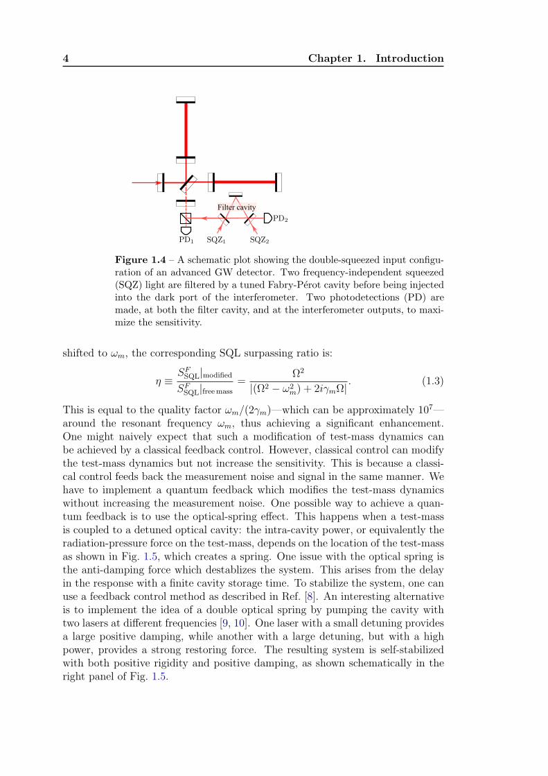
Surpassing the SQL.—From these previous two perspectives on the SQL, we canfind different approaches towards surpassing it, as discussed extensively in theliterature. The first approach is to modify the input and output optics such thatthe shot noise and the radiation-pressure noise are correlated, because the SQLexists only when these two noises are uncorrelated. As shown by Kimble et al [6],by using frequency-dependent squeezed light, the correlation between the shotnoise and the radiation-pressure noise allows the sensitivity to be improved by thesqueezing factor over the entire detection band. The required frequency depen-dence can be realized by filtering frequency-independent squeezed light throughtwo detuned Fabry-Perot cavities before sending into the dark port of the inter-ferometer. Motivated by the work of Corbitt et al. [7], we figure out that such afrequency dependence can also be achieved by filtering two frequency-independentsqueezed lights through a tuned Fabry-Perot cavity. In addition to the detectionat the interferometer dark port, another detection at the filter cavity output isessential to maximize the sensitivity. The configuration is shown schematically inFig. 1.4. An advantage of this scheme is that it only requires a relatively shortfilter cavity (∼ 30 m), in contrast to the km-long filter cavity proposed in Ref. [6].It can be a feasible add-on to advanced GW detectors. This is discussed in detailin Chapter 3.
The second approach is to modify the dynamics of the mechanical oscillator, e.g.,by shifting its eigenfrequency to where the signal is, and amplifying the signal atthe shifted frequency. This is particularly useful for GW detectors in which thependulum frequency of the test masses is very low. If the test-mass frequency is
4 Chapter 1. Introduction
Figure 1.4 – A schematic plot showing the double-squeezed input configu-ration of an advanced GW detector. Two frequency-independent squeezed(SQZ) light are filtered by a tuned Fabry-Perot cavity before being injectedinto the dark port of the interferometer. Two photodetections (PD) aremade, at both the filter cavity, and at the interferometer outputs, to maxi-mize the sensitivity.
shifted to ωm, the corresponding SQL surpassing ratio is:
η ≡SFSQL|modified
SFSQL|freemass
=Ω2
|(Ω2 − ω2m) + 2iγmΩ|
. (1.3)
This is equal to the quality factor ωm/(2γm)—which can be approximately 107—around the resonant frequency ωm, thus achieving a significant enhancement.One might naively expect that such a modification of test-mass dynamics canbe achieved by a classical feedback control. However, classical control can modifythe test-mass dynamics but not increase the sensitivity. This is because a classi-cal control feeds back the measurement noise and signal in the same manner. Wehave to implement a quantum feedback which modifies the test-mass dynamicswithout increasing the measurement noise. One possible way to achieve a quan-tum feedback is to use the optical-spring effect. This happens when a test-massis coupled to a detuned optical cavity: the intra-cavity power, or equivalently theradiation-pressure force on the test-mass, depends on the location of the test-massas shown in Fig. 1.5, which creates a spring. One issue with the optical spring isthe anti-damping force which destablizes the system. This arises from the delayin the response with a finite cavity storage time. To stabilize the system, one canuse a feedback control method as described in Ref. [8]. An interesting alternativeis to implement the idea of a double optical spring by pumping the cavity withtwo lasers at different frequencies [9, 10]. One laser with a small detuning providesa large positive damping, while another with a large detuning, but with a highpower, provides a strong restoring force. The resulting system is self-stabilizedwith both positive rigidity and positive damping, as shown schematically in theright panel of Fig. 1.5.

5
Figure 1.5 – Plot showing the optical spring effect in a detuned opticalcavity. The radiation pressure is proportional to the intra-cavity powerwhich depends on the position of the test mass. The non-zero delay in thecavity response gives rise to an (anti-)damping force. By injecting two laserbeams at different frequencies, this creates a double optical spring and thesystem can be stabilized (right panel).
One limitation with such a modification of the test-mass dynamics mentionedabove is that it only allows a narrow band amplification around the shifted reso-nant frequency. Recently, as realized by Khalili, this limitation can be overcomeby using the frequency dependence of double optical springs, with which the re-sponse function of the free test-mass becomes:
−mΩ2 +K1(Ω) +K2(Ω) (1.4)
with K1 and K2 the optical rigidity. Ideally, if K1(0) + K2(0) = 0, K ′1(0) +
K ′2(0) = 0 and K ′′
1 (0) + K ′′2 (0) = 2m, the inertia of the test mass is canceled,
and a broadband resonance can be achieved. The advantage of this scheme is itsimmunity to the optical loss compared with modifying the input and/or outputoptics. Another parameter regime we are interested in is where two lasers withidentical power are equally detuned, but with opposite signs. Even though thisdoes not surpass the SQL, yet it allows us to follow the SQL at low frequenciesinstead of at one particular frequency in the case shown by Fig. 1.3. This isdiscussed in details in Chapter 4.
A third method is to measure conserved dynamical quantity of the test-mass,also called quantum nondemolition (QND) quantities, which at different timescommute with each other. There will be no associated back action, in contrast tothe case of measuring non-conserved quantities. For a free mass, the conservedquantity is the momentum (speed), and it can be measured, e.g., by adoptingspeed-meter configurations [11–15]. For a high-frequency mechanical oscillator,the conserved quantities are the mechanical quadratures X1 and X2, which aredefined by the equations:
x
δxq≡ X1 cosωmt+ X2 sinωmt,
p
δpq≡ −X1 sinωmt+ X2 cosωmt, (1.5)
with δxq ≡√
~/(2mωm) and δpq ≡√~mωm/2. The quadratures commute with

6 Chapter 1. Introduction
themselves at different times [X1(t), X1(t′)] = [X2(t), X2(t
′)] = 0. To measuremechanical quadratures in the cavity-assisted case, one can modulate the opticalcavity field strength sinusoidally at the mechanical frequency, as pointed out inthe pioneering work of Braginsky [16]. In this case, the measured quantity isproportional to:
E(t)x(t) = E0x(t) cosωmt = E0[X1 + X1 cos 2ωmt+ X2 sin 2ωmt]/2. (1.6)
If the cavity bandwidth is smaller than the mechanical frequency (the so-calledgood-cavity condition), the 2ωm terms will have insignificant contributions to theoutput, and we will measure mostly X1, achieving a QND measurement. However,such a good-cavity condition is not always satisfied, especially in broadband GWdetectors and small-scale devices. Here, we consider a time-domain variationalmethod for measuring the mechanical quadratures, which does not need such agood-cavity condition. By manipulating the output instead of the input field,the measurement-induced back action can be evaded in the measurement data,achieving essentially the same effect as modulating the input field. This approachis motivated by the work of Vyatchanin et al. [17, 18], in which a time-domainvariational method is proposed for detecting GWs with known arrival time.
Macroscopic Quantum Mechanics.—We have been discussing the SQL for mea-suring force with optomechanical devices, and have already seen that the quan-tum dynamics of the mechanical oscillator plays a significant role. A naturalquestion follows: “Can we use such a device to probe the quantum dynamics ofa macroscopic mechanical oscillator, and thereby gain a better understanding ofthe quantum-to-classical transition, and of quantum mechanics in the macroscopicregime? ” The answer would be affirmative if we could overcome a large obstaclein front of us: the thermal decoherence. The coupling between the mechanical os-cillator and high-temperature (usually 300 K) heat bath induces random motionwhich is many order of magnitude higher than that of the quantum zero-pointmotion.
The solution to such a challenge lies in the optomechanical system itself—that is,the optical field. As the typical optical frequency ω0 is around 3 × 10¹⁴ Hz (in-frared), each single quantum ~ω0 has an effective temperature of ~ω0/kB ∼ 15, 000K, which is much higher than the room temperature. This means that the opticalfield is almost in its ground state, with low entropy, and can create an effectivelyzero-temperature heat bath at room temperature. This fact illuminates two ap-proaches to preparing a pure quantum ground state of the mechanical oscillator:(i) Thermodynamical cooling. In this approach, the mechanical oscillator is cou-pled to a detuned optical cavity. There is a positive damping force in the opticaleffect when the cavity is red detuned (i.e., tuned to below the resonant frequencyof the cavity). If the optomechanical damping γopt is much larger than its orig-inal value γm, the the oscillator is settled down in thermal equilibrium with thezero-temperature optical heat bath, as shown schematically in Fig. 1.6. With this

7
Figure 1.6 – Plot showing that the mechanical oscillator is coupled to boththe environmental heat bath with temperature T = 300 K, and to the opticalfield with effective temperature Teff = 0 K. The effective temperature of themechanical oscillator is given by Tm =
γmT+γoptTeff
γm+γopt. This approaches zero
if γopt ≫ γm, which is intuitively expected.
method, many novel experiments have already demonstrated significant reduc-tions of the thermal occupation number of the mechanical oscillator [9, 19–37]. Inthis thesis, we will discuss such a cooling effect in the three-mode optomechanicalinteraction where two optical cavity modes are coupled to a mechanical oscillator(i.e., to a mechanical mode) [refer to Chapter 6 for details]. Due to the opti-mal frequency matching—the frequency gap between two cavity modes is equal tothe mechanical frequency—this method significantly enhances the optomechanicalcoupling, given the same input optical power as the existing two-mode optome-chanical interaction used in those cooling experiments. In addition, it is alsoshown to be less susceptible to classical laser noise. (ii) Uncertainty reductionbased upon information. Since the optical field is coupled to the oscillator, evenif there is no optical spring effect, the information of the oscillator position con-tinuously flows out and is available for detection. From this information, we canreduce our ignorance of the quantum state of the oscillator, and map out a classi-cal trajectory of its mean position and momentum in phase space. The remaininguncertainty of the quantum state will be Heisenberg-limited if the measurementis fast and sensitive enough (i.e., the information extraction rate is high), and thethermal noise induces an insignificant contribution to the uncertainty of the quan-tum state. In this way, the mechanical oscillator is projected to a posterior state,also called the conditional quantum state. The usual mathematical treatment ofsuch a process is by using the stochastic master equation [38–42]. Since we are notinterested in the transient behavior, the frequency-domain Wiener filter approachprovides a neat alternative to obtain the steady-state conditional variance of theoscillator position and momentum (defining the remaining uncertainty). Such anapproach also allows us to include non-Markovian noise, which is difficult to dealwith by using the stochastic master equation. To localize the quantum state inphase space (zero mean position and momentum), one just needs to feed back theacquired classical information with a classical control. There is a unique optimalcontroller that makes the residual uncertainty minimum, and close to that of theconditional quantum state [43].
Due to the intimate connection between the quantity of information in a sys-tem and its thermodynamical entropy, these two approaches merge together inthe case of cavity-assisted cooling scheme. This is motivated by the pioneering

8 Chapter 1. Introduction
work of Marquardt et al. [44] and Wilson-Rae et al. [45]. They showed thatthere is a quantum limit for the achievable occupation number, which is given byγ2/(2ωm)
2. In order to achieve the quantum ground state, the cavity bandwidthγ has to be much smaller than ωm, and this is the so-called good-cavity limit,or resolved-sideband limit. The usual understanding of such a limit is from thethermodynamical point of view, and we point out that it can also be understoodas an information loss. By recovering the information at the cavity output, we canachieve a nearly pure quantum state, mostly independent of the cavity bandwidth.This is explained in Chapter 7.
Preparing non-Gaussian quantum states.—In the above-mentioned situations, thequantum state is Gaussian. By Gaussian, we mean that its Wigner function, whichdescribes the distribution of the position and momentum in phase space, is a two-dimensional Gaussian function. Since it is positive and remains Gaussian, it isdescribable by a classical probability. A unequivocal signature for ‘quantumness’is that the Wigner function can have negative values, e.g. in the well-known‘Schrodinger’s Cat’ state or the Fock state. To prepare these states, it generallyrequires nonlinear coupling between the mechanical oscillator and external degreesof freedom. For optomechanical systems, this can be satisfied if the zero-pointuncertainty of the oscillator position xq is the same order of magnitude as thelinear dynamical range of the optical cavity which is quantified by ratio of theoptical wavelength λ to the finesse F :
λ/(Fxq) . 1. (1.7)
This condition is also the requirement that the momentum kick induced by a singlephoton in a cavity be comparable to the zero-point uncertainty of the oscillatormomentum. Usually, λ ∼ 10−6 m and F ∼ 106, which indicates that xq ∼ 10−12
m and mωm ∼ 10−10. This is rather challenging to achieve with the currentexperimental conditions.
Here we propose a protocol for preparations of a non-Gaussian quantum statewhich does not require nonlinear optomechanical coupling. The idea is to inject anon-Gaussian optical state, e.g., a single-photon pulse created by a cavity QEDprocess [46–48], into the dark port of the interferometric optomechanical device, asshown schematically in Fig. 1.7. The radiation-pressure force of the single photonon the mechanical oscillator is coherently amplified by the classical pumping fromthe bright port. As we will show, the qualitative requirement for preparing anon-Gaussian state becomes:
λ/(F xq) .√Nγ. (1.8)
Here, Nγ = I0 τ/(~ω0) (I0 is the pumping laser power, and ω0 the frequency) isthe number of pumping photons within the duration τ of the single-photon pulse,and we gain a significant factor of
√Nγ, as compared with Eq. (1.7), which makes
this method experimentally achievable.

9
Figure 1.7 – Possible schemes for preparing non-Gaussian quantum statesof mechanical oscillators. The left panel shows the schematic configurationsimilar to that of an advanced GW detector with kg-scale suspended testmasses in both arm cavities. The right panel shows a coupled-cavity schemeproposed in Ref. [31], where a ng-scale membrane is incorporated into ahigh-finesse cavity. In both cases, a non-Gaussian optical state is injectedinto the dark port of the interferometer.
Quantum entanglement.—As one of the most fascinating features of quantum me-chanics, quantum entanglement has aroused many interesting discussions concern-ing the foundation of quantum mechanics, and it also finds tremendous applica-tions in modern quantum information and computing. If two or more subsystemsare entangled, the state of the individual cannot be specified without taking intothe others. Any local measurement on one subsystem will affect others instan-taneously according to the standard interpretation, which violates the so-called“local realism” rooted in the classical physics. The famous “Einstein-Podolsky-Rosen” (EPR) paradox refers to the quantum entanglement for questioning thecompleteness of quantum mechanics [49]. To great extents, creating and testingquantum entanglements has been the driving force for gaining better understand-ing of quantum mechanics.
Interestingly, the optomechanical coupling not only allows us to prepare purequantum states, but also to create quantum entanglements involving macroscopicmechanical oscillators. Since this directly involves macroscopic degrees of free-dom, such entanglements can help us gain insights into the quantum-to-classicaltransition and various decoherence effects which are significant issues in quantumcomputing, and many quantum communication protocols [50].
In the case of a cavity-assisted optomechanical system, it is shown that stationaryEPR-type quantum entanglement between cavity modes and an oscillator [51], oreven between two macroscopic oscillators [52–54] can be created. We also analyzesuch optomechanical entanglement in the three-mode system. The optimal fre-quency matching that enhances the cooling also makes the quantum entanglementeasier to achieve experimentally. Additionally, we investigate how the finite cavitybandwidth that induces the cooling limit influences the entanglement in generaloptomechanical devices. We show that the optomechanical entanglement can besignificantly enhanced if we recover the information at the cavity output. In some

10 Chapter 1. Introduction
cases, the existence of the entanglement critically depends on whether we takecare of the information loss or not.
Motivated by the work of Ref. [54] which shows that the temperature—the strengthof thermal decoherence—only affects the entanglement implicitly, we analyze theentanglement in the simplest optomechanical system with a mechanical oscillatorcoupled to a coherent optical field. Simple though this system is, analyzing theentanglement is highly nontrivial because the coherent optical field has infinitedegrees of freedom. The results are very interesting—the existence of the optome-chanical entanglement is indeed not influenced by the temperature directly, andthe entanglement exists even when the temperature is high and the mechanicaloscillator is highly classical. We obtain an elegant scaling for the entanglementstrength, which only depends on the ratios between the characteristic frequenciesof the optomechanical interaction and the thermal decoherence. This is discussedin detail in Chapter 8.
State verification.—Being able to prepare pure quantum states or entanglementsdoes not tell the full story of an MQM experiment. We need a verification stage,during which the prepared states are probed and verified, to follow up the prepa-ration stage. Suppose the preparation stage finishes at t = 0, the task of theverifier is to make an ensemble measurement of different mechanical quadratures:
Xζ(0) = x(0) cos ζ +p(0)
mωm
sin ζ, (1.9)
with x(0) and p(0) the oscillator position and momentum at t = 0. By buildingup the statistics, we can map out their marginal distributions, from which thefull Wigner function of the quantum state can be constructed. By comparingthe verified quantum state with the prepared one, we can justify the quantumstate preparation procedure. This is a rather routine procedure in the quantumtomography of an optical quantum state. However, this is nontrivial with op-tomechanical devices. Unlike the quantum optics experiments where the opticalquadrature can be easily measured with a homodyne detection, in most casesthat we are interested in, we only measure the position x(t) instead of quadra-tures and the associated back action will perturb the quantum state that we try toprobe. Similar to what is discussed in the first part of this thesis, we also use thetime-domain variational measurement to probe the mechanical quadratures withthe quantum back action evaded from the measurement data. Given a continuousmeasurement from t = 0 to Tint, we can construct the following integral estimator:
X =
∫ Tint
0
dt g(t) x(t) ∝ x(0) cos ζ ′ +p(0)
mωm
sin ζ ′, (1.10)
with cos ζ ′ ≡∫ Tint
0dt g(t) cosωmt and sin ζ ′ ≡
∫ Tint
0dt g(t) sinωmt. In this way, a
mechanical quadrature Xζ′ can be probed. Here, g(t) is some filtering function,which is determined by the time-dependent homodyne phase and also by the way

11
in which data at different times are combined. By optimizing the filtering function,we can achieve a verification accuracy that is below the Heisenberg limit.
A three-stage MQM experiment.—By combining the state preparation and theverification, we can outline a complete procedure for an MQM experiment. Inorder to probe various decoherence effects, and the quantum dynamics, we can in-clude an evolution stage during which the mechanical oscillator freely evolves. Wediscuss such a three-stage procedure: the preparation, evolution, and verificationin advanced GW detectors. The details are in Chapter 11.


Chapter 2
Quantum Theory ofGravitational-Wave Detectors
2.1 Preface
This chapter gives an overview of the quantum theory of gravitational-wave (GW) detectors. It is a modified version of the chapter contributedto a book in progress—Advanced Gravitational-Wave Detectors—editedby David Blair. This chapter is written by Yanbei Chen, and myself.It gives a detailed introduction on how to analyze the quantum noisein advanced GW detectors by using input-output formalism, which isalso valid for general optomechanical devices. It discusses the originof the Standard Quantum Limit (SQL) for GW sensitivity from boththe dynamics of the optical field, and of the test-mass, which leads usto different approaches for surpassing the SQL: (i) creating correlationsbetween the shot noise and back-action noise; (ii) modifying the dynamicsof the test-mass, e.g., through the optical-spring effect; (iii) measuringthe conserved dynamical quantity of the test-mass. For each of theseapproaches, the corresponding feasible configurations to achieve themare discussed in detail. This chapter presents the basic concepts andmathematical tools for understanding later chapters.
2.2 Introduction
The most difficult challenge in building a laser interferometer gravitational-wave(GW) detector is isolating the test masses from the rest of the world (e.g., ran-dom kicks from residual gas molecules, seismic activities, acoustic noises, thermalfluctuations, etc.), whilst keeping the device locked around the correct point ofoperation (e.g., pitch and yaw angles of the mirrors, locations of the beam spots,resonance condition of the cavities, and dark-port condition for the Michelsoninterferometer). Once all these issues have been solved, we arrive at the issuethat we are going to analyze in this chapter: the fundamental noise that arisesfrom quantum fluctuations in the system. A simple estimate, following the steps

14 Chapter 2. Quantum Theory of Gravitational-Wave Detectors
of Braginsky [55], will already lead us into the quantum world — as it will turnout, the superb sensitivity of GW detectors will be constrained by the back-actionnoise imposed by the Heisenberg Uncertainty Principle, when it is applied to testmasses as heavy as 40 kg in the case of Advanced LIGO (AdvLIGO). As Bra-ginsky realized in his analysis, there exists a Standard Quantum Limit (SQL) forthe sensitivities of GW detectors — further improvements of detector sensitivitybeyond this point require us to consider the application of techniques that manip-ulate the quantum coherence of light to our advantage. In this chapter, we willintroduce a set of theoretical tools that will allow us to analyze GW detectorswithin the framework of quantum mechanics; using these tools, we will describeseveral examples in which the SQL can be surpassed.
The outline of this chapter is as follows: In Section 2.3, we will make an order-of-magnitude estimate of the quantum noise in a typical GW detector, from which wecan gain a qualitative understanding of the origin of the SQL; then, in Section 2.4,we will introduce the basic concepts and tools to study the quantum dynamicsof an interferometer, and the associated quantum noise. In Section 2.5, we willanalyze the quantum noise in some simple systems to illustrate the proceduresfor implementing these tools – these simple systems are the fundamental buildingblocks for an advanced GW detector. We will start to study the quantum noise ina typical advanced GW detector in Section 2.6. We will increase the complexitystep by step, each of which is connected in sequence to the simple systems analyzedin the previous section. Section 2.7 will present a rigorous derivation of the SQLfrom a more general context of linear continuous quantum measurements. Thiscan enhance the understanding of the results in the previous section, and also pavethe way to different approaches towards surpassing the SQL. In Section 2.8, wewill talk about the first approach to surpassing the SQL by building correlationsamong quantum noises, and, in Section 2.9, we will illustrate the second approachto beating the SQL by modifying the dynamics of the test mass — in particular, wewill discuss the optical spring effect to realize such an approach. Section 2.10 willpresent an alternative point of view on the origin of the SQL. This will introducethe idea of a speed meter as a third option for surpassing the SQL ,in Section 2.11— two possible experimental configurations of the speed meter will be discussed.Finally, in Section 2.12, we will conclude with a summary of the main results inthis chapter.
2.3 An Order-of-Magnitude Estimate
Here, we first make an order-of-magnitude estimate of the quantum limit for thesensitivity. We assume that test-masses have a reduced mass of m, and it is beingmeasured by a laser beam with optical power I0, and an angular frequency ω0.Within a measurement duration τ , the number of photons is Nγ = I0τ/(~ω0).
2.3. An Order-of-Magnitude Estimate 15
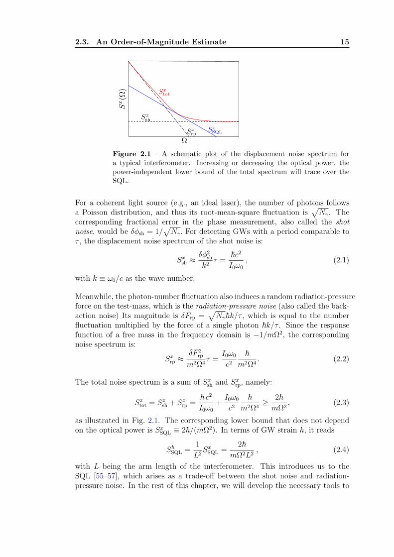
Figure 2.1 – A schematic plot of the displacement noise spectrum fora typical interferometer. Increasing or decreasing the optical power, thepower-independent lower bound of the total spectrum will trace over theSQL.
For a coherent light source (e.g., an ideal laser), the number of photons followsa Poisson distribution, and thus its root-mean-square fluctuation is
√Nγ. The
corresponding fractional error in the phase measurement, also called the shotnoise, would be δϕsh = 1/
√Nγ. For detecting GWs with a period comparable to
τ , the displacement noise spectrum of the shot noise is:
Sxsh ≈ δϕ2
sh
k2τ =
~c2
I0ω0
, (2.1)
with k ≡ ω0/c as the wave number.
Meanwhile, the photon-number fluctuation also induces a random radiation-pressureforce on the test-mass, which is the radiation-pressure noise (also called the back-action noise) Its magnitude is δFrp =
√Nγ~k/τ , which is equal to the number
fluctuation multiplied by the force of a single photon ~k/τ . Since the responsefunction of a free mass in the frequency domain is −1/mΩ2, the correspondingnoise spectrum is:
Sxrp ≈
δF 2rp
m2Ω4τ =
I0ω0
c2~
m2Ω4. (2.2)
The total noise spectrum is a sum of Sxsh and Sx
rp, namely:
Sxtot = Sx
sh + Sxrp =
~ c2
I0ω0
+I0ω0
c2~
m2Ω4≥ 2~mΩ2
, (2.3)
as illustrated in Fig. 2.1. The corresponding lower bound that does not dependon the optical power is Sx
SQL ≡ 2~/(mΩ2). In terms of GW strain h, it reads
ShSQL =
1
L2SxSQL =
2~mΩ2L2
, (2.4)
with L being the arm length of the interferometer. This introduces us to theSQL [55–57], which arises as a trade-off between the shot noise and radiation-pressure noise. In the rest of this chapter, we will develop the necessary tools to

16 Chapter 2. Quantum Theory of Gravitational-Wave Detectors
analyze quantum noise of interferometers from first principles, and to derive theSQL more rigorously. This will allow us to design GW detectors that surpass thislimit.
2.4 Basics for Analyzing Quantum Noise
To rigorously analyze the quantum noise in a detector, we need to study itsquantum dynamics, of which the basics will be introduced in this section.
2.4.1 Quantization of the Optical Field and the Dynamics
For the optical field, the quantum operator of its quantized electric field is
E = u(x, y, z)
∫ +∞
0
dω
2π
√2π~ωAc
[aωe
ikz−iωt + a†ωe+iωt−ikz
]. (2.5)
Here a†ω and aω are the creation and annihilation operators, which satisfy [aω, a†ω′ ] =
2π δ(ω − ω′); A is the cross-sectional area of the optical beam; u(x, y, z) is thespatial mode, satisfying (1/A)
∫dxdy|u(x, y, z)|2 = 1.
For ground-based GW detectors, the GW signal that we are interested in is inthe audio frequency range from 10 Hz to 104 Hz. It creates sidebands on top ofthe carrier frequency of the laser ω0 (3 × 10¹⁴Hz). Therefore, it is convenient tointroduce operators at these sideband frequencies to analyze the quantum noise.The upper and lower sideband operators are a+ ≡ aω0+Ω and a− ≡ aω0−Ω, fromwhich we can define the amplitude quadrature a1 and phase quadrature a2 as:
a1 = (a+ + a†−)/√2, a2 = (a+ − a†−)/(i
√2) . (2.6)
They coherently create one photon and annihilate one photon in the upper andlower sidebands, and this is, therefore, also called the two-photon formalism ([58]).The electric field can then be rewritten as
E(x, y; z, t) = u(x, y, z)
√4π~ω0
Ac[a1(z, t) cosω0t+ a2(z, t) sinω0t] .
where ω is approximated as ω0 and the time-domain quadratures are defined as
a1,2(z, t) ≡∫ +∞
0
dΩ
2π
(a1,2e
−iΩt+ikz + a†1,2eiΩt−ikz
). (2.7)
These correspond to amplitude and phase modulations in the classical limit 1.
1To see such correspondence, suppose the electric field has a large steady-state amplitude A:
E(z, t) = [A+ a1(z, t)] cosω0t+ a2(z, t) sinω0t ≈ A
[1 +
a1(z, t)
A
]cos
[ω0t−
a2(z, t)
A
].

2.4. Basics for Analyzing Quantum Noise 17
free propagation Linear transform
Figure 2.2 – Two basic dynamical processes of the optical field in analyzingthe quantum noise of an interferometer.
After having introduced this quantization, we can look further at the dynamics ofthe optical field. The equations of motion that we will encounter turn out to bevery simple, and only two are relevant, as shown in Fig. 2.2: (i) A free propagation.Given a free propagation distance of L, the new field E ′(t) is
E ′(t) = E(t− τ) , (2.8)
with τ ≡ L/c; (ii) Continuity condition on the mirror surface.
E2(t) =√TE4(t)−
√RE1(t), (2.9)
E3(t) =√RE4(t) +
√TE1(t) , (2.10)
with transmissivity T , reflectivity R, and a sign of convention as indicated in thefigure. These equations relate the optical field before and after the mirror. Dueto the linearity of this system, they are both identical to the classical equationsof motion.
In later discussions, different quantities of the optical field will always be comparedat the same location, and they will all share the same spatial mode. In addition,the propagation phase shift can be absorbed into the time delay. Therefore, we
will ignore the factors u(x, y, z)√
4π~ω0
Ac, and e±ikz, hereafter.
2.4.2 Quantum States of the Optical Field
To determine the expectation value and the quantum fluctuation of the Heisen-berg operators (related to the quantum noise), e.g., ⟨ψ|O|ψ⟩, not only should wespecify the evolution of O, but we also need to specify the quantum state |ψ⟩. Ofparticular interest to us are vacuum, coherent, and squeezed states.
Vacuum state.—The vacuum state |0⟩ is, by definition, the state with no excitationand for every frequency, aΩ|0⟩ = 0. The associated fluctuation is:
⟨0|ai(Ω)aj(Ω′)|0⟩sym = πδijδ(Ω− Ω′), (i, j = 1, 2). (2.11)

18 Chapter 2. Quantum Theory of Gravitational-Wave Detectors
Figure 2.3 – A schematic plot of the electric field and the fluctuations ofamplitude and phase quadrature (shaded area). The left panel shows thetime evolution of E, and the right panel shows E in the space expanded bythe amplitude and phase quadratures (E1, E2).
Equivalently, the double-sided spectral densities 2 for a1,2 are
Sa1(Ω) = Sa2(Ω) = 1, Sa1a2(Ω) = 0 . (2.12)
Coherent state.—The coherent state is defined by [59] as:
|α⟩ ≡ D[α]|0⟩ ≡ exp[∫
dΩ2π(αΩ a
†Ω − α∗
ΩaΩ)]|0⟩ , (2.13)
which satisfies aΩ′|α⟩ = α(Ω′) |α⟩ . The operator D is unitary, so D†D = I. Wecan use this to make a unitary transformation for studying the problem
|ψ⟩ → D†|ψ⟩, O → D†OD , (2.14)
which leaves the physics invariant. This means that the coherent state can bereplaced by the vacuum state, as long as we perform corresponding transforma-tions of O into D†OD. For the annihilation and creation operators, we haveD†(α)aΩD(α) = aΩ+αΩ and D†(α)a†ΩD(α) = a†Ω+α
∗Ω, i.e., the original operators
plus some complex constants.
An ideal single-mode laser with a central frequency ω0 can be modeled as a co-herent state, and αΩ = π a δ(Ω− ω0), with a =
√2I0/(~ω0) and I0 is the optical
power. Under transformation D, the electric field reads [cf. Eq. (2.7)]:
E(t) = [a+ a1(t)] cosω0t+ a2(t) sinω0t , (2.15)
which is simply a sum of a classical amplitude and quantum quadrature fields.This is what we intuitively expect for the optical field from a single-mode laser,namely “quantum fluctuations” superimposed onto a “classical carrier”. In Fig. 2.3,
2For any pair of operators O1 and O2, the double-sided spectral density is defined through
1
2π⟨0|O1(Ω
′)O†2(Ω)|0⟩sym ≡ 1
2π⟨0|O1(Ω
′)O†2(Ω) + O†
2(Ω)O1(Ω′)|0⟩ ≡ 1
2SO1O2(Ω)δ(Ω− Ω′) .

2.4. Basics for Analyzing Quantum Noise 19
Phase squeezingAmplitude squeezing
Figure 2.4 – The fluctuations of the amplitude and phase quadratures(shaded areas) of the squeezed state. The left two panels show the case ofamplitude squeezing; the right two panels show the phase squeezing.
we show E(t) and the associated fluctuations in the amplitude and phase quadra-tures schematically. As we will see later, these fluctuations are attributable to thequantum noise and the associated SQL.
Squeezed state.—A more complicated state would be the squeezed state:
|[χ]⟩ ≡ exp[∫ +∞0
dΩ2π
(χΩ a
†+a
†− − χ∗
Ω a+a−)]|0⟩ ≡ S[χ]|0⟩ . (2.16)
Similar to the coherent-state case, we can also better understand a squeezed stateby making a unitary transformation of the basis through S. By redefining χΩ ≡ξΩ e
−2iϕΩ (ξΩ, ϕΩ ∈ ℜ), for quadratures, this leads to:
S†a1S = a1(cosh ξ + sinh ξ cos 2ϕ)− a2 sinh ξ sin 2ϕ , (2.17)
S†a2S = a2(cosh ξ − sinh ξ cos 2ϕ)− a1 sinh ξ sin 2ϕ . (2.18)
Let us look at two special cases: (i) ϕ = π/2. We have
S†a1S = e−ξa1, S†a2S = eξa2, (2.19)
in which the amplitude quadrature fluctuation is squeezed by e−ξ while the phasequadrature is magnified by eξ; (ii) ϕ = 0. The situation will just be the opposite.Both cases are shown schematically in Fig. 2.4.
2.4.3 Dynamics of the Test-Mass
Similarly, due to the linear dynamics, the quantum equations of motion for thetest masses (relative motion) are formally identical to their classical counterparts:
˙x(t) = p(t)/m, ˙p(t) = I(t)/c+mLh(t). (2.20)
Here x and p are the position and momentum operators, which satisfy [x, p] = i~;I(t)/c is the radiation pressure, which is a linear function of the optical quadra-ture fluctuations; mLh(t) is the GW tidal force. Since the detection frequency(∼100Hz) is much larger than the pendulum frequency (∼1 Hz) of the test-massesin a typical detector, they are treated as free masses.

20 Chapter 2. Quantum Theory of Gravitational-Wave Detectors
2.4.4 Homodyne detection
Figure 2.5 – A schematic plot of two homodyne readout schemes.
In this section, we will consider how to detect the phase shift of the output opticalfield which contains the GW signal. To make a phase sensitive measurement, weneed to measure the quadratures of the optical field, instead of its power. This canbe achieved by a homodyne detection in which the output signal light is mixed witha local oscillator, thus producing a photon flux that depends linearly on the phase(i.e., on the GW strain). Specifically, for a local oscillator L(t) = L1 cosω0t +L2 sinω0t and output b(t) = b1(t) cosω0t+ b2(t) sinω0t, the photocurrent is i(t) ∝|L(t) + b(t)|2 = 2L1b1(t) + 2L2b2(t) + · · · . The rest of the terms, represented by“· · · ”, contain either frequency components that are strictly DC and around 2ω0,and terms quadratic in b. In such a way, we can measure a given quadraturebζ(t) = b1(t) cos ζ + b2(t) sin ζ , by choosing the correct local oscillator, such thattan ζ = L2/L1.
In order to realize the above ideal superposition, there are two possible schemes:introducing the local oscillator from the injected laser (external scheme as shownin the right panel of Fig. 2.5); or intentionally offsetting the two arms at the verybeginning, with a very small phase mismatch, which results in the so-called DCreadout scheme, as shown in the left panel of Fig. 2.5.
2.5 Examples
Before analyzing the quantum noise in an advanced interferometric GW detector,it is illustrative to first consider three examples: (i) A test mass coupled to an op-tical field in free space; (ii) A tuned Fabry-Perot cavity with a movable end mirroras the test mass; (iii) A detuned Fabry-Perot cavity with a movable end mirror.These three examples summarize the main physical processes in an advanced GWdetector. Understanding them will not only help us to get familiar with the tools

2.5. Examples 21
for analyzing quantum noise in a GW detector, but can also provide intuitivepictures which will be useful in understanding more complicated configurations.
2.5.1 Example I: Free Space
Figure 2.6 – A schematic plot of the interaction between the test massand a coherent optical field in free space (left); and the associated physicalquantities (right).
The model is shown schematically in Fig. 2.6. The laser-pumped input opticalfield can be written as [cf. Eq. (2.15)]:
Ein(t) = [√
2I0/(~ω0) + a1(t)] cosω0t+ a2(t) sinω0t. (2.21)
The output field Eout(t) is simply:
Eout(t) = Ein(t− 2τ − 2x/c) , (2.22)
with a delay time τ ≡ L/c. We define output quadratures b1 and b2 through:
Eout(t) = [√2I0/(~ω0) + b1(t)] cosω0t+ b2(t) sinω0t. (2.23)
Since the displacement of the test mass is small, and the uncertainty of ω0x/c ismuch smaller than unity, we can make a Taylor expansion of Eq. (2.22) in a seriesof ω0x/c. Up to the leading order, we obtain the following input-output relations:
b1(t) = a1(t− 2τ) , (2.24)
b2(t) = a2(t− 2τ)− 2
√2I0~ω0
ω0
cx(t− τ) , (2.25)
where, for simplicity, we have assumed that ω0L/c = nπ, with n an integer.
The equation of motion for the test-mass displacement x is simply:
m¨x(t) = Frp(t) +1
2mLh(t) . (2.26)
Here we have chosen an inertial reference frame, as indicated in Fig. 2.6, such thatthe gravitational tidal force is equal to 1
2mLh(t); the radiation-pressure force Frp
on the test-mass is given by:
Frp(t) = 2A4π
|Ein(t− τ)|2 = 2I0c
[1 +
√2~ω0
I0a1(t− τ)
], (2.27)

22 Chapter 2. Quantum Theory of Gravitational-Wave Detectors
where in the second equality we have kept to the first order of the amplitudequadrature. There is a DC component in the radiation-pressure force, whichcan be balanced in the experiment (e.g., by the wire tension in the case of asuspended pendulum). We are interested in the perturbed part, proportional tothe amplitude quadrature, which accounts for the radiation-pressure noise.
We can solve Eqs. (2.24), (2.25) and (2.26) by transforming them into the fre-quency domain, after which we obtain:
b(Ω) = M a(Ω) + D h(Ω) , (2.28)
where a = (a1, a2)T, b = (b1, b2)
T (superscript T denoting transpose); the trans-
fer matrix M and transfer vector D can be read off from the following explicitexpression of Eq. (2.28):[
b1(Ω)
b2(Ω)
]= e2iΩτ
[1 0−κ 1
] [a1(Ω)a2(Ω)
]+
[0
eiΩτ√2κ
]h(Ω)
hSQL
, (2.29)
with
κ =8I0ω0
mc2Ω2, hSQL =
√8~
mΩ2L2. (2.30)
As we can see, the GW signal is contained in the output phase quadrature b2. Itcan be decomposed into signal and noise components:
b2(Ω) = ⟨b2(Ω)⟩+∆b2(Ω) , (2.31)
where ⟨b2(Ω)⟩ is the expectation value of the output, which is proportional tothe GW signal h, and ∆b2 is the quantum fluctuation with zero expectation. Bydefining ⟨b2(Ω)⟩ ≡ T h, we introduce the following quantity:
T = eiΩτ√2κ
1
hSQL
, (2.32)
which is the transfer function from the GW strain h to the output phase quadra-ture. This particular form indicates that the output phase modulation is propor-tional to the GW strain, delayed by a constant time τ . The noise part
∆b2(Ω) = e2iΩτ a2(Ω)− e2iΩτκ a1(Ω) , (2.33)
contains two parts: (i) the first one is the shot noise nsh ≡ e2iΩτ a2, which arisesfrom the phase-quadrature fluctuation of the input optical field and has a flatspectrum [cf. Eq. (2.12)]:
Ssh(Ω) = 1; (2.34)
and (ii) the second one is the radiation-pressure noise nrp ≡ (−e2iΩτκ a1). Thisarises from the amplitude-quadrature fluctuation, and has the following noisespectrum:
Srp(Ω) = κ2 , (2.35)

2.5. Examples 23
with a frequency dependence of 1/Ω4.
Given the coherent state of the input optical field, the amplitude and phase-quadrature fluctuations are not correlated. Therefore, we can obtain the totalnoise spectrum simply by summing up Ssh and Srp. By normalizing with thetransfer function T , the signal-referred noise spectrum can be written as:
Sh(Ω) =1
|T |2S∆b2
(Ω) =
[1
κ+ κ
]h2SQL
2≥ h2SQL. (2.36)
The shot-noise contribution (first term) is inversely proportional to the opticalpower (κ ∝ I0) and the radiation-pressure noise (second term) is proportional toI0. The balance between them gives the SQL for detecting GWs with this simpledevice. We will find that although this model is simple, it summarizes the mainfeatures of a GW detector.
2.5.2 Example II: A Tuned Fabry-Perot Cavity
Figure 2.7 – A schematic plot of the tuned-cavity model (left); and theassociated physical quantities (right).
Now we consider the case of a tuned Fabry-Perot cavity. In Fig. 2.7, we showthe model schematically. In comparison with the previous case, an additionalmirror with transmissivity (of power) T , and reflectivity R, are placed in frontof the test-mass, in effect “wrapping” around the original system. We define thenew input and output optical fields E ′
in,out, in a similar way to that of Ein,out, by
simply replacing a, b with new amplitude and phase quadratures α, β. We need todetermine a new input-output relation between α1,2 and β1,2. From the continuitycondition on the front mirror surface [cf. Eqs. (2.9) and (2.10)], we have:
Ein =√REout +
√TE ′
in , (2.37)
E ′out =
√TEout −
√RE ′
in . (2.38)
Correspondingly, a, b are related to new quadrature fields α, β by:
a =√R b+
√T α , (2.39)
β =√T b−
√R α . (2.40)
Together with Eq. (2.28), it would be straightforward to obtain the new input-output relation. Generally, the expression is rather cumbersome. We will focus
24 Chapter 2. Quantum Theory of Gravitational-Wave Detectors
on the case in which the transmissivity T is small (i.e., a high-finesse cavity).In addition, since the GW sideband frequency Ω we are interested in is around100 Hz, Ω τ is much smaller than unity even when the cavity length L is 4 km.Therefore, we can make a Taylor expansion of the new input-output relation asa series of the dimensionless quantities T and Ω τ . Up to the leading order, thisleads to:[
β1(Ω)
β2(Ω)
]= e2iϕ
[1 0
−K 1
] [α1(Ω)α2(Ω)
]+ e−iϕ
[0√2K
]h
hSQL
. (2.41)
We have introduced:
ϕ ≡ arctan(Ω/γ), K ≡ 2γ ιcΩ2(Ω2 + γ2)
, (2.42)
with the cavity bandwidth γ ≡ Tc/(4L), parameter ιc ≡ 8ω0Ic/(mLc), and intra-cavity power Ic ≡ 4I0/T .
The same as the previous free-space case, we need to read out the phase quadratureof the output field which contains the GW signal. The corresponding signal-referred noise spectrum Sh has a similar form to the previous free-space case, butwith κ replaced by K [cf. Eq. (2.36)], i.e.:
Sh(Ω) =
[1
K+K
]h2SQL
2≥ h2SQL. (2.43)
For frequencies around Ω ∼ γ, the shot noise spectrum almost decreases by afactor of 1/T 2 in comparison with the free-space case. This is attributable tothe coherent amplification of the optical power and the signal. The additionalmirror serves as a quantum feedback, which allows signals to build up coherently,whilst noise adds up incoherently over time. [On the other hand, a classicalfeedback will not normally increase the signal-to-noise ratio, as feeding back whatis already known will not increase knowledge.] For frequencies Ω > γ, the shotnoise increases as Ω2, rather than remaining constant in the previous case. This isdue to the non-zero response time of the cavity, and signal with frequencies higherthan γ are averaged out. Therefore, the cavity bandwidth roughly determines thedetection bandwidth.
2.5.3 Example III: A Detuned Fabry-Perot Cavity
If the cavity is not tuned, as shown schematically in Fig. 2.8, namely, ω0τ =θ + nπ (θ = 0) with n an integer, the free propagation will not only induce aphase shift, but also a rotation of the quadratures. This simply arises from thefollowing fact: given a free-space propagation of τ , and from the relation Eout(t) =

2.5. Examples 25
Figure 2.8 – A schematic plot of a detuned cavity; and the associatedphysical quantities (right). Here, θ is the detuned phase.
Ein(t− τ), the quadrature evolves as:[b1(Ω)
b2(Ω)
]= eiΩτ
[cosω0τ − sinω0τsinω0τ cosω0τ
] [a1(Ω)a2(Ω)
], (2.44)
which is a delay and rotation.
Correspondingly, Eqs. (2.39) and (2.40) are modified:
a =√RR2θ b+
√T Rθ α , (2.45)
β =√T Rθ b−
√R α , (2.46)
where Rθ is the rotation matrix, defined as
Rθ ≡(
cos θ − sin θsin θ cos θ
). (2.47)
Similarly, if the detuned phase is small, with θ ≪ 1, we can make a Taylorexpansion of these equations in series of θ, T and Ω τ . After some manipulation,the new input-output relation can be expressed in the following compact form:
β(Ω) =1
C[M α(Ω) + D h(Ω)], (2.48)
where
C = Ω2[(Ω + iγ)2 −∆2] + ∆ιc, (2.49)
M =
[−Ω2(Ω2 + γ2 −∆2)−∆ ιc 2γ∆Ω2
−2γ∆Ω2 + 2γιc −Ω2(Ω2 + γ2 −∆2)−∆ιc
], (2.50)
D =
[∆Ω
(−γ + iΩ)Ω
]2√γιc
hSQL
, (2.51)
with detuning frequency ∆ ≡ θ/τ . Here we have ignored the tiny frequency-dependent phase correction Ω θ/ω0. Unlike in the previous two cases, the GWsignal here appears in both amplitude and phase quadratures. To readout theGW signal, we can make a homodyne detection of a certain output quadrature:
βζ(Ω) = β1(Ω) cos ζ + β2(Ω) sin ζ. (2.52)

26 Chapter 2. Quantum Theory of Gravitational-Wave Detectors
Given a coherent state input, the corresponding signal-referred noise spectrumdensity is
Sh(Ω) =(cos ζ, sin ζ)MMT(cos ζ, sin ζ)T
|D1 cos ζ +D2 sin ζ|2, (2.53)
with D1,2 being the components of the vector D. This expression recovers theprevious two cases: (i) the tuned cavity, by setting ∆ = 0, and phase quadraturemeasurement ζ = 0; (ii) the free-space case, by setting the cavity bandwidthγ → ∞. We will postpone discussing the physical significance of this formulauntil we consider a signal-recycled GW detector, which can actually be mappedinto a detuned Fabry-Perot cavity.
2.6 Quantum Noise in an Advanced GW Detec-
tor
Figure 2.9 – A schematic plot of an advanced GW detector. The beamsplitter (BS) splits the laser light into two beams. The internal test-mass(ITM) and end test-mass (ETM) with optical coatings on their surface formthe Fabry-Perot arm cavities which amplifies both the signal and opticalpower. The power recycling mirror (PRM) can further increase the circu-lating power. The signal-recycling mirror (SRM) folds the signal back intothe interferometer, and it significantly enriches the dynamics of the system,as discussed in the main text.
After having introduced some basic principles and examples, we are now readyto analyze the quantum noise of a typical advanced GW detector: a Michelsoninterferometer with Fabry-Perot arm cavities, a power-recycling mirror (PRM),and a signal-recycling mirror (SRM). This is shown schematically in Fig. 2.9.
To make a direct one-to-one correspondence between the input-output relation ofan advanced GW detector and the three examples we have considered, we will

2.6. Quantum Noise in an Advanced GW Detector 27
gradually introduce important optical elements, and discuss them in the follow-ing sequence: (i) a simple Michelson interferometer with only end test-masses(Sec. 2.6.1); (ii) a power-recycled interferometer with both power-recycling mir-ror and arm cavities (Sec. 2.6.2); (iii) a power- and signal-recycled interferometer(Sec. 2.6.3).
2.6.1 Input-Output Relation of a Simple Michelson Inter-ferometer
Figure 2.10 – A schematic plot of a simple Michelson interferometer (left);and its mathematical model with propagating optical fields (right).
A simple Michelson interferometer is shown schematically in Fig. 2.10. Ideally,the interferometer is set up to have identical arms, so that at the zero workingpoint of the interferometer (i.e., when locked on a dark fringe), fields enteringfrom each port will only return to that port. The carrier light enters and exitsfrom the common (bright) port, while the differential port remains dark. Thedifferential motion of the test mass xA− xB, which contains the GW signal causesa differential phase modulation, and therefore induces an output signal out of thedifferential (dark) port, at which we make homodyne detections.
We follow steps similar to those in Sec. 2.5.1 to derive the input-output relationhere. As we will see, the input-output relation of the differential displacementwe are interested in is exactly the same as the free-space scenario considered inSec. 2.5.1. The laser-pumped input optical field into the common port is:
Einc (t) = [
√2I0/(~ω0) + c1(t)] cosω0t+ c2(t) sinω0t. (2.54)
With no laser pumping, the input field into the differential port is simply:
Eind (t) = [a1(t) cosω0t+ a2(t) sinω0t] . (2.55)

28 Chapter 2. Quantum Theory of Gravitational-Wave Detectors
The fields, after passing through the half-half beam splitter, and while propagatingtowards ETMA and ETMB, are:
EinA,B(t) =
Einc (t)∓ Ein
d (t)√2
. (2.56)
The fields returning from the ETM are
EoutA,B(t) = Ein
A,B(t− 2τ − 2xA,B/c) , (2.57)
where τ ≡ L/c is the time for light to propagate from the beam splitter to eachof the ETMs. To the leading order in xA,B, we have:
Eoutd (t) =
EoutB (t)− Eout
A (t)√2
≡ [b1(t) cosω0t+ b2(t) sinω0t] , (2.58)
with
b1(t) = a1(t− 2τ), (2.59)
b2(t) = a2(t− 2τ)−√
2I0~ω0
ω0
cxd(t− τ), (2.60)
where we have assumed ω0L/c = nπ, with n an integer; and have defined thedifferential-mode motion:
xd(t) ≡ xB(t)− xA(t) . (2.61)
Radiation-pressure forces acting on the two test-masses have both common anddifferential components, which are proportional to c1 and a1 respectively. If testmasses have nearly the same mass, m, then c1 (a1) will only induce common-mode (differential-mode) motion. Mathematically, we have, up to leading orderin fluctuations/modulations:
FA,B(t) = 2I0c
[1 +
√~ω0
I0
c1(t− τ)∓ a1(t− τ)√2
]. (2.62)
For the differential mode:
FB(t)− FA(t) = 2
√2~ω0I0c
a1(t− τ) . (2.63)
This means that the motion of the differential mode under both the radiation-pressure force and the tidal force, F h
A,B = ∓mLh(t)/2, from GW is:
m ¨xd(t) = FB(t)− FA(t)+FhB(t)−F h
A(t) = 2
√2~ω0I0c
a1(t− τ)+mLh(t) . (2.64)

2.6. Quantum Noise in an Advanced GW Detector 29
Eqs. (2.59), (2.60) and (2.64) are identical to Eqs. (2.24), (2.25) and (2.26), if weidentify the previous 2 x by the differential displacement xd here. Since the GWsignal also increases by a factor of 2, due to the differential motion of two arms,the signal strength will not change. Therefore, the signal-referred noise spectrumobtained in the free-space case also applies [cf. Eq. (2.36)], namely:
Sh(Ω) =
[1
κ+ κ
]h2SQL
2, (2.65)
except for the fact that here:
κ =4I0ω0
mc2Ω2, hSQL =
√4
mΩ2L2. (2.66)
2.6.2 Interferometer with Power-Recycling Mirror and ArmCavities
Figure 2.11 – A schematic plot of a Michelson interferometer with a power-recycled mirror (PRM) and additional ITMs to form arm cavities (left). Thecorresponding propagating fields are indicated in the right diagram.
In order to decrease the shot noise, we need to increase the optical power. Itwould be difficult to achieve a high optical power by solely increasing the inputpower. Instead, we can add a power-recycling mirror, as first proposed by [60](see Fig. 2.11). The output optical field from the common port gets coherentlyreflected back into the interferometer, and amplifies the circulation power. Sincewe are only concerned with the optical field in the differential port, the effect of thePRM can easily be included by simply replacing the input I0 in Ec
in(t) (Eq. 2.54)by:
I ′0 ≡4
TPRM
I0 , (2.67)
where TPRM is the power transmissivity of the PRM. Further improvement of thesensitivity comes from the arm cavities formed by the ITMs and ETMs. Thesecavities are tuned on resonance, further increasing the optical power circulating in

30 Chapter 2. Quantum Theory of Gravitational-Wave Detectors
the arms, and also coherently amplifying the GW signal by increasing the effectivearm length.
The input-output relation at the differential port also has the same form as thetuned Fabry-Perot cavity discussed in Sec. 2.5.2. This can be shown as follows:The new optical fields Ein′
A and Eout′A are related to Ein
A and EoutA simply by:
EinA =
√RIE
outA +
√TIE
in′
A , (2.68)
Eout′
A =√TIE
outA −
√RIE
in′
A , (2.69)
where√RI and
√TI are the reflectivity and transmissivity, respectively, of the
ITM. Similar relations hold for the fields propagating in the arm cavity B. Thesenew fields are connected to the new input Ein′
c and Ein′
d by:
Ein′
A,B =Ein′
c (t)∓ Ein′
d (t)√2
. (2.70)
In addition, the new output in the differential port is:
Eout′
d =Eout′
B (t)− Eout′A (t)√
2. (2.71)
The relations between the new inputs Ein′
d , Eout′
d and outputs Eind , E
outd , at the
differential port, are simply defined by:
Eind =
√RIE
outd +
√TIE
in′
d , (2.72)
Eout′
d =√TIE
outd −
√RIE
in′
d . (2.73)
These have the same form as Eqs. (2.37) and (2.38). Therefore, as long as we areonly concerned with the fields at the differential port, the new input and outputare related to the previous ones without arm cavities in a similar way as that of asingle tuned Fabry-Perot cavity. There is only one difference: in the single tunedcavity analysis, we assumed the front mirror is fixed, while in the GW detector,both ITMs and ETMs can move and the relative motion is detected, which hasa reduced mass of m/2 in each arm. By further taking into account a factor oftwo increase in the sensitivity from two arms, the resulting signal-referred noisespectrum reads [cf. Eq. (2.43)]:
Sh(Ω) =
[1
K+K
]h2SQL
2, (2.74)
with
K ≡ 2γ ιcΩ2(Ω2 + γ2)
, hSQL =
√8~
mΩ2L2. (2.75)
The cavity bandwidth, γ ≡ TIc/(4L), and the parameter ιc are the same as inEq. (2.42), but with Ic ≡ 8I0/(TPRMTI), which is enhanced by both the power-recycling and arm cavities. To illustrate this sensitivity, we can choose the follow-ing specifications for different parameters (close to those of the AdvLIGO): mass

2.6. Quantum Noise in an Advanced GW Detector 31
10 100 10000.1
1
10
100
f @HzD
Sh
hq
SQL
Figure 2.12 – The GW strain-referred sensitivity of an advanced GW de-tector with power-recycled mirror and arm cavities, given the specificationsdetailed in the main text. Here, we have normalized the spectrum by hq,which is defined to be hSQL at 100 Hz.
of individual test mass m = 40 kg, intra-cavity optical power Ic = 800 kW, armcavity length L = 4 km, optical angular frequency ω0 = 1.9×10¹⁵s−1 (wavelengthequal to 1µ m), arm cavity bandwidth γ/(2π) = 100 Hz. The correspondingsensitivity is shown in Fig. 2.12, and it achieves the SQL round 100 Hz.
2.6.3 Interferometer with Signal-Recycling
Figure 2.13 – A schematic plot of a Michelson interferometer with a power-(PRM) and signal-recycled mirrors (SRM) and additional ITMs to formarm cavities (left). The corresponding propagating fields are indicated inthe right-hand diagram, with θ being the detuned phase.
Now we are ready to analyze the quantum noise in an advanced GW detectorwith both power- and signal- recycling. The schematic plot of the configuration isshown in Fig. 2.13, where a signal-recycling mirror is added onto the differentialport, as first proposed by [61, 62]. After previously introducing all the techniques,

32 Chapter 2. Quantum Theory of Gravitational-Wave Detectors
Figure 2.14 – Mapping from a three-mirror cavity to a two-mirror cavityby defining the effective transmissivities (teff , t
′eff) and reflectivities (reff , r
′eff)
of the signal-recycling cavity.
the effect on the detector sensitivity also becomes apparent. With the same idea,we can relate the new input and output fields Ein′′
d , Eout′′
d to the Ein′
d , Eout′
d fieldsanalyzed in the previous section. The relation reads:
Ein′
d (t) =√RSE
out′
d (t− 2θ/ω0) +√TSE
in′′
d (t− θ/ω0) , (2.76)
Eout′′
d (t) =√TSE
out′
d (t− θ/ω0)−√RSE
in′′
d (t) , (2.77)
with θ the detuned phase and RS and TS the reflectivity and transmissivity ofthe SRM, respectively. The corresponding quadratures will undergo rotationsidentical to those shown in the single detuned cavity analysis [cf. Eqs. (2.45)and (2.46)]. The expression for this input-output relation is very lengthy andcomplicated [8, 63]. We will follow the approach in Ref. [64] and map the entiresignal-recycled interferometer into a single detuned cavity, which will then allowus to directly use the results obtained in Sec. 2.5.3.
The idea behind this mapping is based upon the fact that the length, LSR, of thesignal-recycling cavity formed by the ITMs and the SRM is, of the order of 10meters, which is very short compared with km long arm cavity. The propagationphase shift of the sidebands around 100 Hz, eiΩLSR , is negligible [65, 66]. As shownschematically in Fig. 2.14, the signal-recycling cavity can be replaced by one mirrorwith a set of effective reflectivities and transmissivities, which are related to TS,Iand RS,I by:
reff = −√RS +
√RI e
2iθ
1 +√RIe2iθ
, t′eff =
√RI +
√RS RI e
2iθ
1 +√RS RI e2iθ
, (2.78)
teff = t′eff =
√TS TI e
iθ
1 +√RS RI e2iθ
. (2.79)
From the resonant condition of the effective cavity:
r′effe2iΩresL/c = 1, (2.80)
we can define its effective bandwidth γeff and detuning ∆eff through:
Ωres ≡ −∆eff − i γeff . (2.81)

2.6. Quantum Noise in an Advanced GW Detector 33
Up to the leading order of TI , ∆eff and γeff can be expressed in terms of√TS,I ,
√RS,I
and θ through
∆eff =2√RSγI sin 2θ
1 +RS + 2√RS cos 2θ
, γeff =(1−RS)γI
1 +RS + 2√RS cos 2θ
, (2.82)
with the bandwidth of the arm cavity γI ≡ c TI/(4L).
10 100 10000.1
1
10
100
f @HzD
Sh
hq
SQL
Figure 2.15 – The GW strain-referred sensitivity of a signal-recycling GWdetector given a phase-quadrature detection ζ = π/2. The solid curve cor-responds to the RSE scheme with θ = π/2 and
√RS = 0.6. The dashed
curve shows the case with θ = 1.1 and√RS = 0.9.
After this equivalent mapping into a single detuned cavity, it is straightforward toobtain the input-output relation for the signal-recycling interferometer, throughthe following replacement in Eq. (2.48):
γ → γeff , ∆ → ∆eff . (2.83)
For illustration, we assume an ideal phase-quadrature detection with ζ = π/2; thecorresponding GW strain-referred sensitivity is given by [cf. Eq. (2.53)]:
Sh(Ω) =4γ2eff(ιc +∆effΩ
2)2 + [∆effιc + Ω2(γ2eff −∆2eff + Ω2)]2
4γeffιcΩ2(γ2eff + Ω2)h2SQL. (2.84)
One interesting example is when θ = π/2, giving
γeff =1 +
√RS
1−√RS
γ, ∆eff = 0 . (2.85)
The resulting noise spectrum is the same as the previous case without signal-recycling, but with an increased detection bandwidth (a factor of (1+
√RS)/(1−√
RS)). This is the so-called Resonant-Sideband-Extraction (RSE) scheme whichwill be implemented in AdvLIGO. The spectrum is shown in Fig. 2.15. In gen-eral, θ = π/2 and we also show the noise spectrum in the case for a SR cavity

34 Chapter 2. Quantum Theory of Gravitational-Wave Detectors
detuned phase θ = 1.1. As we can see, there are two minima in the sensitivitycurve. Interestingly, they surpass the SQL around the most sensitive frequency(∼ 100Hz for given specifications). To gain a better insight into these featureswhich surpasses the SQL, we need to examine the origin of the SQL from a moregeneral picture of linear continuous measurements. Not only will it allow us tounderstand this particular example, but it can also provide an insight into theSQL, and thus help us to find other approaches to surpass it.
2.7 Derivation of the SQL: a General Argument
Probe Detector
Figure 2.16 – A schematic model of a linear continuous measurement pro-cess.
Throughout the previous discussions, we have learnt that there are two types ofnoise, namely shot noise and radiation-pressure noise. They together give riseto the SQL of the detector sensitivity. Actually, the SQL exists in general linearcontinuous measurements, and it is directly related to the fundamental HeisenbergUncertainty Principle [57]. We will elaborate on this point in this section.
The model of a typical measurement process is shown schematically in Fig. 2.16.The signal – a classical force G (e.g., from the GW) is driving the probe (e.g., thetest mass) which is in turn coupled to an external detector (e.g., the optical field).The detector reads out the probe motion by monitoring its displacement x, andat the same time it exerts a back-action force F onto the conjugate momentum ofthe probe. The signal force G can then be extracted from the detector output Y ,which contains both the signal and the fundamental measurement noise Z (i.e.,the shot noise). Mathematically, the displacement-referred output Y , i.e., themeasurement result, can be written as:
Y (t) = x0 + Z(t) +
∫ t
−∞dt′Rxx(t− t′)[F (t′) +G(t′)]. (2.86)
Here x0 is the free-evolution value of the probe displacement when the detector isdetached, and it has the following two-time commutator:
[x0(t), x0(t′)] = −i~Rxx(t− t′) , (2.87)
where Rxx(t) is the response function of the probe to the external force. Here, werequire that the detector is tunable, and has a parameter ϵ, with:
Zϵ(t) =ϵ
ϵ0Zϵ0(t) , Fϵ(t) =
ϵ0ϵFϵ0(t) . (2.88)
2.7. Derivation of the SQL: a General Argument 35
The fact that Y (t) is the measurement result itself dictates that
[Y (t), Y (t′)] = 0 , (2.89)
because measuring Y (t) continuously should not impose any additional noise [57].In addition, since Z and F are operators that belong to a different system (thedetector) from the probe, they both commute with the probe displacement x0. Itis therefore required that the two-time commutator of Z and F terms in Y mustcancel from x0. In fact, because Z and F have different scalings in ϵ, and becausethe cancelation must happen at all orders of ϵ, we can obtain:
[Z(t), Z(t′)] = [F (t), F (t′)] = 0 , [Z(t), F (t′)] = i~ δ(t− t′) . (2.90)
This indicates that the shot noise and the back-action noise do not commute atthe same moment. In the frequency domain, this can be written as:
[Z(Ω), Z(Ω′)] = [F (Ω), F (Ω′)] = 0 , [Z(Ω), F (Ω′)] = 2π i~ δ(Ω− Ω′) . (2.91)
If we introduce the single-sided (cross) spectral densities SZZ(Ω), SFF (Ω) andSZF (Ω), the above commutation relations dictate the Heisenberg UncertaintyPrinciple:
SZZ(Ω)SFF (Ω)− |SZF (Ω)|2 ≥ ~2 . (2.92)
This generally will not set a bound on the noise spectrum in measuring the probedisplacement [cf. Eq. (2.86)] which is given by:
Sx(Ω) = SZZ(Ω) + 2ℜ[Rxx(Ω)SZF (Ω)] + |Rxx(Ω)|2SFF (Ω) (2.93)
with Rxx(Ω) the Fourier transform of Rxx(t). However, when there is no correla-tion between the shot noise and the back-action noise, namely SZF = 0, it inducesthe SQL for the displacement measurement:
Sx(Ω) ≥ 2|Rxx(Ω)|√SZZ(Ω)SFF (Ω) ≥ 2~|Rxx(Ω)| ≡ Sx
SQL. (2.94)
In the case of GW detection, the external force is the GW tidal force on the testmasses and we have G(t) = mLh(t) (m is the reduced mass). Therefore, the SQLfor the GW signal-referred sensitivity reads
ShSQL =
2~m2Ω4L2|Rxx(Ω)|
. (2.95)
For a free mass, Rxx(Ω) = −1/(mΩ2); this gives the free-mass SQL:
ShSQL =
2~mΩ2L2
, (2.96)
which justifies the order-of-magnitude estimate we obtained in Eq. (2.4).
From the above derivation, we immediately realize that there are two possibleapproaches to surpassing the free-mass SQL: (i) Creating correlations between the

36 Chapter 2. Quantum Theory of Gravitational-Wave Detectors
shot noise Z and the back-action noise F with non-zero SZF . Correspondingly,the inequality in Eq. (2.94) is not satisfied, and the total noise spectrum willnot be bounded by the SQL; (ii) Modifying the dynamics of the probe: Thefree-mass SQL will no longer be relevant if the probe has a different responseto the external force than the free mass. In particular, for an oscillator with aresonance frequency ωm and decay rate γm, the response function reads Rxx(Ω) =1/[−m(Ω2 − ω2
m + iγmΩ)], and then around resonance frequency:
ShSQL|oscillatorShSQL|freemass
=
√(Ω2 − ω2
m)2 + γ2mΩ
2
Ω2
∣∣∣Ω=ωm
=γmωm
. (2.97)
The free-mass SQL can therefore be surpassed by a significant amount of themechanical quality factor ωm/γm around its resonance frequency. We will explorethese two approaches in detail in the next two sections.
2.8 Beating the SQL by Building Correlations
In this section, we will focus on the first approach to beat the SQL, by creat-ing correlations between the shot noise and the back-action noise. This can beachieved by: (i) signal-recycling; (ii) squeezed input; (iii) variational readout. Thedetails of these methods will be discussed.
2.8.1 Signal-recycling
In the previous section [cf. Sec. 2.6.3], we showed that the signal-recycled interfer-ometer can be mapped into a detuned cavity, in which the amplitude and phasequadratures will rotate and mix with each other. When their fluctuations arereflected back to the test mass by the signal-recycling mirror, both will contributeto the radiation-pressure noise, similarly for the shot noise, which will have contri-butions from both fluctuations. Therefore, the shot noise and radiation-pressurenoise naturally acquire correlations. In the case of phase-quadrature readout, itcan be shown that this correlation is given by [64]:
SZF = ~∆eff(∆
2eff + 3γ2eff − Ω2)
2γeff(γ2eff + Ω2). (2.98)
This accounts for the two minima in the sensitivity curve, which surpass the SQL,as shown in Fig. 2.15.

2.8. Beating the SQL by Building Correlations 37
Figure 2.17 – A schematic plot of the frequency-dependent squeezed in-put configuration. A frequency-independent squeezed light, filtered by twodetuned Fabry-Perot cavities in sequence, produces the required frequencydependence.
2.8.2 Squeezed input
As pointed out in the pioneering work of [6], a frequency-dependent squeezedinput can be used to surpass the SQL; in this case, the shot noise and radiation-pressure noise are naturally correlated as a result of the correlation between theamplitude and phase quadratures of the input squeezed light. To illustrate thispoint, we will only look at the scheme discussed in Sec. 2.6.2 without a signal-recycling mirror. It can be easily generalized and extended to general schemes.Given a squeezed input, the amplitude and phase quadrature will be transformedaccording to Eqs. (2.17) and (2.18). As shown in [6], if the squeezing angle ϕ hasthe following frequency dependence:
ϕ(Ω) = −arccotK(Ω), (2.99)
the amplitude and phase fluctuations are squeezed at low and high frequencies,respectively, and the noise spectrum will be reduced by a overall squeezing factorof e2q, namely:
Shsqz = e−2q
[K +
1
K
]h2SQL
2, (2.100)
which surpasses the SQL at around the most sensitive frequencies, as indicated inFig. 2.18. It is possible to achieve a frequency-dependent squeezing, as prescribedin Eq. (2.99), because different sideband frequencies all represent different degreesof freedom, and therefore squeezing them in different ways is totally allowed. Inpractice, one must invent the right device that generates such a frequency depen-dence. This usually implies devices with a certain time scale that is comparableto the detection band of the detector, which is very long compared with usualquantum optical devices.

38 Chapter 2. Quantum Theory of Gravitational-Wave Detectors
10 100 10000.1
1
10
100
f @HzD
Sh
hq
SQL
Figure 2.18 – The GW strain-referred sensitivity of a frequency-dependentsqueezing input interferometer (solid curve). The squeezing factor is e−2q =0.1. The other specification is the same as Fig. 2.12.
Kimble et al. invented one such device – a detuned Fabry Perot cavity. ForFabry-Perot Michelson interferometers, they showed that a squeezing angle ofarctanK can be generated by feeding a frequency-independent squeezed light intotwo consecutive Fabry-Perot cavities, each with a perfect end mirror, and pre-scribed values of detuning and bandwidth. The specifications for the filter cavityparameters can be obtained by using the technique given in the Appendix of [13].This technique is valid for general schemes, such as a signal-recycling configura-tion, shown explicitly in [67], in which the noise spectrum is also reduced by thesqueezing factor for the entire detection band.
2.8.3 Variational Readout: Back-Action Evasion
Figure 2.19 – A schematic plot of the variational-readout configuration.The output is filtered by two detuned Fabry-Perot cavities before the de-tection.

2.8. Beating the SQL by Building Correlations 39
10 100 10000.1
1
10
100
f @HzD
SQL
Sh
hq
Figure 2.20 – The GW strain-referred sensitivity of a variational-readoutscheme (solid curve). The low-frequency back-action noise is completedevaded, thus achieving a sensitivity limited only by shot noise.
Another natural way to build correlations is to measure a certain combination ofthe amplitude quadrature b1 and phase quadrature b2 at the output, namely:
bζ = b1 cos ζ + b2 sin ζ
= (a1 cos ζ + a2 sin ζ)− a1K sin ζ +√2K h
hSQL
sin ζ. (2.101)
The shot noise (a1 cos ζ + a2 sin ζ) and the radiation-pressure noise a1K sin ζ hasnon-zero correlation. If the detection angle ζ has the following frequency depen-dence:
ζ(Ω) = arccotK(Ω), (2.102)
we can completely evade the effect of back-action, and obtain a shot-noise onlysensitivity, namely:
Shvar =
h2SQL
2K. (2.103)
Such back-action- evading scheme was first invented by Vyatchanin et al. ina time domain formalism [17, 18], aimed at detecting GWs with known arrivaltime. The above frequency-domain formalism was developed by Kimble et al., andit is valid for all possible stationary signals. The required frequency dependencycan be achieved in a similar way to that of frequency-dependent squeezing, i.e., byfiltering the output through detuned Fabry-Perot cavity, as shown schematicallyin Fig. 2.19. The specifications for the filter cavities can also be obtained by usingthe results in Ref. [13]. The corresponding sensitivity curve is shown in Fig. 2.20.
2.8.4 Optical losses
In the above discussions, we have assumed an ideal lossless situation. However,in reality, there are multiple channels in which losses can be introduced. These

40 Chapter 2. Quantum Theory of Gravitational-Wave Detectors
include the scattering and losses in the optical elements, and the non-zero trans-mission of the end mirrors. These optical losses will introduce uncorrelated vac-uum fluctuations, and destroy the quantum coherence. They can be modeled byan overall reduction of the field amplitude by
√1− ϵ, and then an introduction
of√ϵ for the vacuum:
b→√1− ϵb+
√ϵn . (2.104)
Here n is associated with the uncorrelated vacuum fluctuations. They will notonly affect the injected squeezed state but also the output field, which underminesthe sensitivity. As shown by Kimble et al., the squeezed-input configuration isreasonably robust against optical loss as long as the filter cavities have a lengthcomparable to the arm cavity (∼ 4 km). However, the variational-readout schemeis very susceptible to the optical losses. If we apply the condition in Eq. (2.102),the noise spectrum with the output loss [cf. Eq. (2.104)] is:
Shloss(Ω) =
[ϵ
2(1− ϵ)K sin2 ζ+
1
2K
]h2SQL. (2.105)
At low frequencies, K ∼ Ω−2 and sin2 ζ ∼ Ω4, and thus the first term scales asΩ−2. This means that the loss will severely affect the low-frequency sensitivity.In addition, as shown by Kimble et al., around the frequency where the SQL isattained for a conventional scheme without a signal-recycling mirror, the SQLbeating ratio of a variational-readout scheme with loss is given by:
µ ≡
√ShSQL
Shvar
≈ 4√ϵ, (2.106)
only if the interferometer can manage a factor of 1/√ϵ times stronger optical
power. Given a typical loss of 0.01, this produces a factor of 0.3 and a power 10times greater, which is rather challenging. Therefore, a low-loss optical setup isessential for implementation.
2.9 Optical Spring: Modification of Test-Mass
Dynamics
Apart from building correlations, as shown by Eq. (2.97), the free-mass SQLcan also be surpassed by modifying the dynamics of the test-mass. One mightexpect that this will require a significant modification of the topology of currentGW detectors. As it turns out, a detuned signal-recycling interferometer natu-rally achieves this. This is intimately connected to the rotation of the amplitudeand phase quadrature in the signal-recycling cavity, which produces correlationsbetween the shot noise and radiation-pressure noise. As we have previously men-tioned, the radiation pressure force not only depends on the amplitude quadrature,

2.9. Optical Spring: Modification of Test-Mass Dynamics 41
but also on the phase quadrature. Since the latter contains the test-mass displace-ment, it induces a position-dependent force and modifies the test-mass dynamics;This phenomenon is also called the “optical-spring” effect. A similar idea, butwith a different configuration, was first proposed by [68], and is the so-called“optical bar” GW detector.
2.9.1 Qualitative Understanding of Optical-Spring Effect
Figure 2.21 – The optical power as a function of cavity detuning ∆ (left).A double optical spring, Ktot(Ω) = K1(Ω)+K2(Ω), which has both positiverigidity and damping (right). The black curve (right) shows a parametricplot of the optical spring K(Ω) as a function of detuning.
The optical-spring effect can be understood qualitatively by looking at the caseof a single detuned cavity. The displacement of the end mirror (test-mass) x willchange the intra-cavity power Ic, which in turn changes the radiation-pressureforce. In the adiabatic limit, the intra-cavity power as a function of x reads:
Ic(x) =γ2Imax
c
γ2 + [∆ + (ω0x/L)]2, (2.107)
which is shown in the left panel of Fig. 2.21. Since the radiation-pressure force isequal to F (x) = Ic(x)/c, such a position-dependent force will introduce a rigidity,which is minus the derivative of the force −dF (x)/dx, around the equilibriumpoint x = 0. Depending on the sign of the detuning, it will create either negativeor positive rigidity. In the case of a detuned signal-recycling configuration forAdvLIGO, a strong optical-spring effect can shift the pendulum frequency of 1Hz up to the detection band. Around the new resonant frequency, we can surpassthe free-mass SQL. This actually accounts for the low-frequency dip in Fig. 2.15.One can refer to Ref. [63] for a detailed discussion of the mechanical resonancedue to this optical-spring effect.
Due to a delayed response of the intra-cavity power to the test-mass motion, theoptical spring also has a friction component. For ∆ < 0, such a delayed response
42 Chapter 2. Quantum Theory of Gravitational-Wave Detectors
gives a positive damping, which pumps energy out of the test mass. For ∆ > 0,the damping is negative, which will destabilize the system. Using the input-outputrelation derived in Sec. 2.5.3, one can easily determine the expression for an opticalspring in the frequency domain as:
K(Ω) = −2Icω0
Lc
∆
(Ω−∆+ iγ)(Ω + ∆+ iγ). (2.108)
For sideband frequencies Ω < ∆, γ, we can perform a Taylor expansion and obtain
K(Ω) =2Icω0
Lc
[∆
γ2 +∆2+
2iγ∆
(γ2 +∆2)2Ω
]≡ Kopt − iγoptΩ. (2.109)
We have introduced the rigidity Kopt (real part of K) and the damping γopt (imag-inary part). As we can see, the positive (negative) rigidity is always accompaniedby a negative (positive) damping. In either case, the system is unstable. Tostabilize the system, one can use a feedback control as described by [8]. An inter-esting alternative is to implement the idea of a double optical spring, by pumpingthe cavity with two lasers at different frequencies [9, 10]. One laser with a smalldetuning provides a large positive damping while another with a large detune,but with a high power, provides a strong restoring force. The resulting system isself-stabilized with both positive rigidity and positive damping, as shown schemat-ically in the right panel of Fig. 2.21.
2.10 Continuous State Demolition: Another View-
point on the SQL
In the previous section [cf. Sec. 2.7], we derive the SQL by focusing on thequantum nature of the detection (the optical field). In this section, we will derivethe SQL from another perspective — continuous state demolition. This will guideus to finding new approaches to surpassing the SQL.
In the Heisenberg picture, suppose we attempt to measure the position of a freemass successively at discrete times separated by τ . We measure x at time t1, thenright after t1, the quantum state of the test mass is characterized by a standarddeviation comparable to the individual-measurement error ϵ, or:
∆x(t1 + 0) = ϵ . (2.110)
The value of ϵ decreases indefinitely as individual-measurement sensitivity in-creases. Applying free-mass quantum mechanics for the duration of t ∈ (t1, t2),we have
[x(t1 + 0), x(t2 − 0)] =i~(t2 − t1)
m=i~τm
. (2.111)

2.11. Speed Meters 43
The decreasing ϵ will lead to an increasing variance in ∆x(t2 − 0) right beforethe second measurement. This is because the Heisenberg Uncertainty Principledictates that:
∆x(t1 + 0) ·∆x(t2 − 0) ≥ ~τ/(2m) , (2.112)
and
∆x(t2 − 0) >~τ2mϵ
. (2.113)
This large variance in the x(t2 − 0) distribution will be reduced down to ϵ by thesubsequent measurement on x(t2) — but at the price of demolishing a quantumstate with a large spread of x(t2) into classical superpositions of quantum stateswith much smaller variances.
If the successive measurements are done without coordination, i.e., if the metersthat collapse the mirror’s states at t1 and t2 are not correlated, then the demolitionwill cause an additional noise, because the new center of the wavefunction aftercollapse is randomly chosen among a distribution with variance ∆x(t2 − 0). If wenow characterize the noise of each individual measurement in position, we obtain,
∆x ≥ max
(ϵ,
~τ2mϵ
)≥√
~τ2m
. (2.114)
This provides us with the scale of the standard quantum limit. In fact, if forany pulse with duration τ , which can vary at all scales, our measurement error isalways:
∆x ∼√
~τ2m
, (2.115)
then the noise spectral density of the device is characterized by:
Sx(Ω) ∼ ~2mΩ2
. (2.116)
Therefore, the SQL can be traced back to the fact that the test mass positions atdifferent times do not commute with themselves [cf. Eq. (2.111)].
2.11 Speed Meters
This alternative viewpoint on the SQL naturally brings us to the idea of a speedmeter, which measures the speed (momentum) instead of the position of the testmass. Since the momentum of a free mass is a conserved dynamical quantity,and its Heisenberg operators at different times commute with each other, one canmeasure it continuously without imposing additional noise, thus allowing us tosurpass the SQL.

44 Chapter 2. Quantum Theory of Gravitational-Wave Detectors
Apart from beating the SQL, other more practical issues that make the speedmeter attractive are the following: (i) the previous schemes require frequency-dependent squeezing or readout which has led to the requirement of two extrakm-scale filter cavities — a high cost in practical construction; (ii) the high valueof K at low frequencies leads to a strong sensitivity to optical losses. As it turnsout, these issues are resolved simultaneously when we try to build a speed meter,which has a constant sensitivity to the speed of test masses in low frequencies —the requirement for frequency dependence on squeezing and readout quadraturetherefore vanishes. In fact, if we imagine an interferometer with a constant κ[cf. Eq. (2.29)] or K [cf. Eq. (2.41)] in the input-output relation, it will indeedrespond to the speed of the mirror position.
Here we will discuss two realizations, both found as prototypes in the early pa-pers of [11, 69], but later gradually deformed into the shape of km-scale laserinterferometers [12–14].
2.11.1 Realization I: Coupled cavities
BSLaser
Photodetector
Arm cavity A
Arm
cav
ity
B
PRM
Sloshing cavityClosed port
ETM Sloshing cavity
Figure 2.22 – A schematic plot of a speed-meter configuration with coupledcavities. A sloshing cavity is added after the dark port. Such a configurationcan be mapped into a three-mirror cavity as schematically shown in theright-hand panel, forming a pair of coupled cavities.
A possible Michelson variant is shown in Fig. 2.22. An additional sloshing cavity isadded after the interferometer output. It has an input-mirror with transmissivityTs and a totally-reflected end mirror. There is another extraction mirror (with atransmissivity of T0) between the interferometer output and the sloshing cavity,through which we read out the signal. This configuration emerges from the two-resonator model of Braginsky and Khalili, where it was pointed out that if tworesonators are coupled, then a sloshing of signal light between the two cavitiescancel each other out, leaving only a sensitivity to the change in mirror position,

2.11. Speed Meters 45
i.e., the speed. The characteristic sloshing frequency is given by:
ωs =
√Tsc
2L. (2.117)
The explicit expression for the response function of the output to the test massmotion can be found by analyzing the input-output relation, giving:
T (Ω) =ω0
L
iΩ
Ω2 − ω2s + iγΩ
, (2.118)
with γ ≡ 4T0c/L due to the extraction mirror. This can also be derived by fittingthe speed meter into the two-resonator model. We can map the speed meterconfiguration into a three-mirror cavity, as shown schematically in Fig. 2.22. The‘x’ corresponds to the differential motion of the end test masses. The left cavitycorresponds to the power-recycled Michelson interferometer, and the right cavityis still the sloshing cavity. The optical fields are summarized by two cavity modesα and β. Their equations of motion are:
α(t) + γ α(t) = iωs β(t) + iω0
Lx(t), (2.119)
β(t) = iωs α(t). (2.120)
We have assumed that both cavity modes are on resonance with respect to thecarrier laser frequency. In addition, we attribute the decay only to the left cavity(due to the extraction mirror). The coupling between the two modes is manifestedby the sloshing terms on the right hand side (proportional to ωs). Solving theabove equation in the frequency domain will immediately give the result in Eq.(2.118).
The GW strain sensitivity of such a configuration can be derived by using theinput-output formalism that we have introduced. Given a frequency-independentsqueezing (phase squeezing factor e−2q), the result is [refer to Ref. [13] for moredetails]:
Sh =
[e−2q
2Ksm
+e2q(cot ζ −Ksm)
2
2Ksm
]h2SQL , (2.121)
where ζ is the readout quadrature angle, and
Ksm =16ω0γIc
mcL[(Ω2 − ω2s)
2 + γ2Ω2]. (2.122)
The first term in Sh is the shot-noise term, and the second is the radiation-pressurenoise. At low frequencies, Ksm is almost a constant. By choosing cot ζ = Ksm(0),the low-frequency radiation-pressure (back-action) can be completely evaded. Weshow the resulting GW strain sensitivity in Fig. 2.23.
There is, however, a subtle issue: the original Braginsky and Khalili argumentstated that momentum can be measured without additional noise — yet in speed

46 Chapter 2. Quantum Theory of Gravitational-Wave Detectors
10 100 10000.1
1
10
100
f @HzD
Sh
hq
SQL
Figure 2.23 – The GW strain-referred sensitivity of the speed meter schemeshown in Fig. 2.22. We have chosen γ/2π = 210 Hz, ωs/2π = 180 Hz andIc = 800 kW. The dotted curve is the case without a phase-squeezed input,and the solid curve has e−2q = 0.1 (a 10 dB squeezing).
meters, we still need back-action evasion: is this still consistent? The answer isyes, because when speed is coupled to an external observable, it ceases to be pro-portional to the conserved, canonical momentum. Here, we sketch a mathematicalproof by Khalili. Suppose the Lagrangian is:
L =1
2mx2 + αa1x , (2.123)
which is the model of a speed meter: the time derivative of the external observablea1 represents the sloshing. Here, the quantity α is a coupling constant. This isequivalent to:
L =1
2mx2 − αa1x , (2.124)
where the coupling becomes a speed coupling, but the canonical momentum isgiven by:
p =∂L∂x
= mx− αa1 , (2.125)
which is conserved, but differs from the kinetic momentum, mx. This meansthat a meter that measures speed must add a constant αa1/m, in order to evadethe back-action. Note that this is a constant combination between the outputphase quadrature and amplitude quadrature — therefore, back-action evasion isstraightforward without requiring additional filtering. This is manifested by thefact that Ksm is almost constant at low frequencies.
2.11.2 Realization II: Zero-area Sagnac
Another possible speed meter configuration is a zero-area Sagnac interferometer,which is shown schematically in Fig. 2.24. This has a different optical topology

2.12. Conclusions 47
Figure 2.24 – A schematic plot of a Sagnac-type speed meter configuration.
from the Michelson scheme, where the light travels through two opposite loops inthe interferometer. To understand its response to the test-mass motion, we canlook at a single trip. The light propagating towards arm A first picks up a phaseshift proportional to ETMA, displacement xA(t), and it accumulates another phaseshift due to motion of ETMB, but at t−τ (τ is the delay time). A similar situationholds for the light propagating towards arm B, but with the roles of ETMA andETMB swapped. When they recombine at the beam splitter, the total phase shiftis simply:
ϕtot(t) ∝ xA(t) + xB(t− τ)− xB(t)− xA(t− τ) ≈ [ ˙xA(t)− ˙xB(t)]τ. (2.126)
It naturally has no response to a static change in arm length, but only to the dif-ferential speed of the two test masses. Therefore, it is a natural speed meter. Thishas been recognized by the GW community, but connection with the “QuantumNondemolition” (QND) speed meter, has never been made. As shown in [14], theGW strain sensitivity of such a configuration is identical to the previous coupled-cavities configuration.
2.12 Conclusions
We have introduced the basic concepts for studying the quantum dynamics andassociated quantum noise of an interferometric GW detector. Different insightsinto the origin of the SQL allow us to find out possible approaches towards sur-passing it. In particular, we have considered modifying the input/ouput opticsusing either frequency-dependent squeezing or a variational readout, and modi-fying the test mass dynamics through the optical spring effect; and measuring aQND observable of the test mass by using a speed meter. This not only serves as

48 Chapter 2. Quantum Theory of Gravitational-Wave Detectors
a review of advanced configurations for future GW detectors, but it additionallyprovides valid examples to help clarify many subtle issues in continuous quantummeasurement.

Chapter 3
Modifying Input Optics: DoubleSqueezed-input
3.1 Preface
In this chapter, we consider improving the sensitivity of future interfero-metric GW detectors by modifying their input optics. In particular, wediscuss simultaneously injecting two squeezed light, filtered through a res-onant Fabry-Perot cavity, into the dark port of the interferometer. Thisis motivated by the work of Corbitt et al. [7], in which a similar scheme,but with a single squeezed light was proposed and analyzed. Here weshow that the extra squeezed light, together with an additional homo-dyne detection suggested previously by Khalili [70], allows a reduction ofquantum noise over the entire detection band. To motivate future imple-mentations, we take into account a realistic technical noise budget for theAdvanced LIGO (AdvLIGO), and numerically optimize the parametersof both the filter and the interferometer for detecting gravitational-wavesignals from two important astrophysics sources: neutron-star–neutron-Star (NS-NS) binaries and Bursts. Assuming the optical loss of the ∼ 30m filter cavity to be 10 ppm per bounce, and 10dB squeezing injection,the corresponding quantum noise with optimal parameters decreases by afactor of 10 at high frequencies and goes below the technical noise at lowand intermediate frequencies. This is a joint research by Farid Khalili,Yanbei Chen and myself. It is published in Phys. Rev. D 80, 042006(2009).
3.2 Introduction
During the last decade, several laser interferometric gravitational-wave (GW) de-tectors including LIGO [3], VIRGO [4], GEO600 [5] and TAMA [71] have beenbuilt and operated almost at their design sensitivity, aiming at extracting GWsignals from various astrophysical sources. At present, the development of next-generation detectors, such as AdvLIGO [72], is also under way, and the sensitivities

50 Chapter 3. Modifying Input Optics: Double Squeezed-input
of these advanced detectors are anticipated to be limited by quantum noise overalmost the whole observational band from 10 Hz to 104 Hz. At high frequencies,the dominant quantum noise is photon shot noise, caused by phase fluctuation ofthe optical field; while at low frequencies, the radiation-pressure noise, due to theamplitude fluctuation, dominates and it exerts a noisy random force on the probemasses. These two noises, if uncorrelated, will impose a lower bound on the noisespectrum, which is called the Standard Quantum Limit (SQL). In terms of theGW strain h ≡ ∆L/L, this limit is given by
SSQLh =
8~mΩ2L2
. (3.1)
This can also be derived from the fact that position measurements of the free testmass do not commute with themselves at different times [73].
Filter cavity
|SQZÚ
|SQZÚ
AHD
EM IM
PRM
LM
MHD
PBS
ETMB
ITMB
ETMA ITMA
SRM
Figure 3.1 – Schematic plot of the proposed configuration. Two squeezedlight beams s, p are injected from both side of the filter cavity rather thanthe one which was considered in Refs. [7, 70]. The signal is detected bythe main homodyne detector (MHD) and an additional detector (AHD) isplaced at the idle port of the filter cavity.
The existence of the SQL was first realized by Braginsky in the 1960’s [55, 74].Since then, various approaches have been proposed to beat the SQL. One recog-nized by Braginsky is to measure conserved quantities of the probe masses, alsocalled Quantum Nondemolition (QND) quantities. This can be achieved, e.g. byadopting “speed meter” configurations [11–15, 69], which measure the conservedquantity—momentum rather than the position. An alternative is to change thedynamics of the probe mass, e.g. by using optical rigidity [75, 76], in which casethe above-mentioned free mass SQL is no longer relevant. As shown by Buonannoand Chen [8, 63, 64], optical rigidity exists in signal-recycled (SR) interferometricGW detectors; therefore we can beat the SQL without radical redesigns of the

3.2. Introduction 51
existing topology of the interferometers. Another approach is to modify the in-put and/or output optics of the interferometers, such that photon shot noise andradiation-pressure noise are correlated. After the initial paper by Unruh [77], thiswas further developed by other authors [6, 7, 17, 78–83]. A natural way to achievethis is injecting a squeezed vacuum state, whose phase and amplitude fluctuationsare correlated, into the dark port of the interferometer. With great advancementsin preparation of the squeezed state [84, 85], squeezed-input interferometers willbe promising candidates for third-generation GW detectors. As elaborated in thework of Kimble et al. [6], frequency-dependent squeezing is essential to reducethe quantum noise at various frequencies of the observation band. In addition,they demonstrated that this can be realized by filtering the frequency-independentsqueezed vacuum state through two detuned Fabry-Perot cavities before sendinginto the interferometer. Their results were extended by Purdue and Chen [13]who discussed the filters for general cases.
Another method, which also uses an additional filter cavity and squeezed state, butin a completely different way, was proposed by Corbitt, Mavalvala, and Whitcomb(hereafter referred to as CMW) [7]. They proposed to use a tuned optical cavityas a high-pass filter for the squeezed state. This scheme does not create the noisescorrelation, but instead, renders their spectral densities frequency-dependent. Athigh frequencies, the phase-squeezed vacuum state gets reflected by the filter andenters the interferometer such that high-frequency shot noise is reduced; whileat low frequencies, ordinary vacuum transmits through the filter and enters theinterferometer, thus low-frequency radiation-pressure noise remains unchanged.One significant advantage is that the squeezed vacuum state does not really enterthe filter cavity, and thus it is less susceptible to the optical losses. However,it does not perform so well as hoped, and there is a noticeable degradation ofsensitivity in the intermediate-frequency range. One of us — Khalili [70] pointedout that this has to do with the quantum entanglement between the optical fieldsat the two ports of the filter cavity. Equivalently, it can be interpreted physicallyas follows: some information about the phase and amplitude fluctuations flowsout from the idle port of the filter cavity and the remaining quantum state whichenters the interferometer is not pure. In order to recover the sensitivity, the filtercavity needs to have a low optical loss, such that this information can be collectedby an additional homodyne detector (AHD) at the idle port. Given an achievableoptical loss of the filter cavity ∼ 10 ppm per bounce, Khalili showed that we canobtain the desired sensitivity at intermediate frequencies. A natural extensionof this scheme is to send an additional squeezed vacuum state into the idle portof the filter cavity, such that the low-frequencies radiation-pressure noise is alsosuppressed. The corresponding configuration is shown schematically in Fig. 3.1,where two squeezed vacuum states s and p are injected from two ports of thefilter cavity, and some ordinary vacuum state n leaks into the filter due to opticallosses. By optimizing the squeezing angles of these squeezed states, we will showthat the resulting quantum noise is reduced over the entire observational band.

52 Chapter 3. Modifying Input Optics: Double Squeezed-input
The outline of this chapter is as follows: in Sec. 3.3, we will calculate the quantumnoises in this double squeezed-input CMW scheme with AHD (later referred to asCMWA). We will use the same notation as in Ref [64], which enables us to extendthe results in Ref. [70] to the case of signal-recycled interferometers easily. In Sec.3.4, we numerically optimize the parameters of this new scheme, as employed inthe search for GW signals from NS-NS binaries and Bursts. Finally, we summarizeour results in Sec. 3.5. For simplicity, we will neglect the optical losses inside themain interferometer, but we do consider the losses from the filter cavity, and alsofrom the non-unity quantum efficiency of the photodiodes. The losses from themain interferometer are not expected to be important, as shown in Refs. [6, 8, 70].The main quantities used in this paper are listed in Table 3.1.
Table 3.1 – Main quantities in this paper.
Quantity Value for Estimates DescriptionsΩ GW frequencyc 3.0× 10⁸ m/s Speed of lightω0 1.8× 10¹⁵ s−1 Laser frequencym 40 kg Test massL 4 km Arm cavity lengthIc 840 kW Optical powerιc =
8ω0IcmLc
(2π × 100)3s−3
γarm 2π × 100 s−1 Cavity bandwithrSR SRM reflectivityϕSR Phase detuning of SR cavityδ Effective detuningγ Effective bandwidthϕ MHD homodyne angleζ AHD homodyne angleLf 30 m Filter cavity Length
γI,E,L =T 2I,E,L
2τf
γf = γI + γE + γL Filter cavity bandwith
ri (i = s, p) (ln 10)/2 (10dB) Squeezing factorsθi (i = s, p) Squeezing angles

3.3. Quantum noise calculation 53
3.3 Quantum noise calculation
3.3.1 Filter cavity
In this section, we will derive single-sided spectral densities of the two outgoingfields a and q as shown in Fig. 3.1. From the continuity of optical fields, we canrelate them to the ingoing fields, which include two squeezed vacuum states s , pand one ordinary vacuum n entering from the lossy mirror (LM) [70]. Specifically,we have
a(Ω) = RI(Ω)s(Ω) + T (Ω)p(Ω) +AI(Ω)n(Ω), (3.2)
q(Ω) = RE(Ω)p(Ω) + T (Ω)s(Ω) +AE(Ω)n(Ω). (3.3)
Here a = (aA, aφ)T, q = (qA, qφ)
T are amplitude and phase quadratures (sub-script A stands for amplitude and φ for phase). In our case, the carrier light beamis resonant inside the filter cavity. Therefore, the effective amplitude reflectivityR, transmissivity T and loss A can be written as,
RI(Ω) =γI − γE − γL + iΩ
γf − iΩ, RE(Ω) =
γE − γI − γL + iΩ
γf − iΩ, (3.4a)
T (Ω) =−2
√γIγE
γf − iΩ, (3.4b)
AI(Ω) =−2
√γIγL
γf − iΩ, AE(Ω) =
2√γEγL
γf − iΩ, (3.4c)
where γf ≡ γI + γE + γL. They satisfy the following identities:
|RI(Ω)|2 + |T (Ω)|2 + |AI(Ω)|2 = |RE(Ω)|2 + |T (Ω)|2 + |AE(Ω)|2 = 1, (3.5a)
R∗I (Ω)T (Ω) +RE(Ω)T ∗(Ω) +A∗
I (Ω)AE(Ω) = 0. (3.5b)
If the input and end mirrors of the filter cavity are identical, namely γI = γE, wewill have RI,RE ∼ 1 and T ∼ 0 when Ω ≫ γf and RI,RE ∼ 0 and T ∼ 1 whenΩ ≪ γf . Therefore, the squeezed vacuum s enters the interferometer at highfrequencies while p becomes significant mostly at low frequencies. By adjustingthe squeezing factor and angle of these two squeezed fields, we can reduce boththe high-frequency shot noise, and the low-frequency radiation-pressure noise,simultaneously.
To calculate the noise spectral densities, we assume that these two squeezed vac-uum sates have frequency-independent squeezing angles θi (i = s, p), and can berepresented as follows:
s = R(rs, θs)v s , p = R(rp, θp)v p , (3.6)
54 Chapter 3. Modifying Input Optics: Double Squeezed-input
with
R(r, θ) ≡(
cosh r − cos θ sinh r − sin θ sinh r− sin θ sinh r cosh r + cos θ sinh r
). (3.7)
Here r is the squeezing factor, and v i = (viA, viφ)T are ordinary vacuums with
single-sided spectral densities: SA(Ω) = Sφ(Ω) = 1, SAφ(Ω) = 0 [6].
The noise spectral densities of the two filter-cavity outputs can then be writtenas
Saa(Ω) = |RI(Ω)|2R(2rs, 2θs) + |T (Ω)|2R(2rp, 2θp) + |AI(Ω)|2I, (3.8)
Sqq(Ω) = |RE(Ω)|2R(2rp, 2θp) + |T (Ω)|2R(2rs, 2θs) + |AE(Ω)|2I, (3.9)
Saq(Ω) = RE(Ω)T ∗(Ω)R(2rp, 2θp) +R∗I (Ω)T (Ω)R(2rs, 2θs)
+ AE(Ω)A∗I (Ω)I, (3.10)
where Saq(Ω) is the cross correlation between two outputs; I is the identity matrixand
Si(Ω) =
(SA,i(Ω) SAφ,i(Ω)SAφ,i(Ω) Sφ,i(Ω)
), (3.11)
with i = aa, qq, aq, whose elements are single-sided spectral densities.
3.3.2 Quantum noise of the interferometer
According to Ref. [64], the input-output relation, which connects the ingoingfields a and the GW signal h with the outgoing fields b, for a signal-recycledinterferometer can be written as:
b =1
M
(C a +D
h
hSQL
). (3.12)
In the above equation,
M = [δ2 − (Ω + iγ)2]Ω2 − δ ιc, (3.13)
and C is the transfer function matrix, with elements:
C11 = C22 = Ω2(Ω2 − δ2 + γ2) + δ ιc, (3.14a)
C12 = −2γ δΩ2, C21 = 2γ δΩ2 − 2γ ιc, (3.14b)
where ιc ≡ 8ω0Ic/(mcL). The elements of the transfer function vector D are
D1 = −2δ√γ ιc Ω, D2 = −2(γ − iΩ)
√γ ιc Ω. (3.15a)

3.3. Quantum noise calculation 55
The effective detuning δ, and bandwidth γ, are given by:
δ =2 rSR γarm sin(2ϕSR)
1 + r2SR + 2 rSR cos(2ϕSR), (3.16a)
γ =(1− r2SR)γarm
1 + r2SR + 2 rSR cos(2ϕSR), (3.16b)
where rSR is the amplitude reflectivity of the signal-recycling mirror (SRM), andϕSR is the phase detuning of the SR cavity. If the main homodyne detector (MHD)measures:
bϕ(Ω) =√η [sinϕ bA(Ω) + cosϕ bφ(Ω)] +
√1− η v(Ω), (3.17)
where ϕ is the homodyne angle and v is the additional vacuum state due to thenon-unity quantum efficiency of the photodiode, and then the corresponding h-referred quantum-noise spectral density can be written as:
Sh(Ω) = h2SQL
(sinϕ cosϕ)C SI C†(sinϕ cosϕ)T + 1−η
η|M |2
(sinϕ cosϕ)D D†(sinϕ cosϕ)T. (3.18)
This can be minimized by adjusting the squeezing angle θ of s and p. We canestimate the optimal θ qualitatively from the asymptotic behavior of the resultingnoise spectrum. At very high frequencies (Ω ≫ γ), from Eq. (3.2), a ∼ s andthus:
Sh(Ω) ∝ cosh(2rs) + cos[2(ϕ+ θs)] sinh(2rs). (3.19)
If the squeezing angle of s :
θs =π
2+ nπ − ϕ, (3.20)
where n is integer, we achieve the optimal case, namely Sh ∝ e−2rs . Similarly, atvery low frequencies (Ω ≪ γ), we have a ∼ p and the spectral density Sh ∝ e−2rp
if
θp = arctan
[2 cosϕ sin β
cos(β − ϕ) + 3 cos(β + ϕ)
]. (3.21)
More accurate values for optimal θs,p can be obtained numerically, as we will showin the next section. Given optimal θs,p, the sensitivity of this double squeezed-input scheme improves at both high and low frequencies. However, for the samereason as in the case of single squeezed-input that the two outputs of the filtercavity are entangled [70], this double squeezed-input scheme does not performwell in the intermediate frequency range. To recover the sensitivity, we need touse an additional homodyne detector (AHD) at the idle port E of the filter cavity.The corresponding measured quantity is:
qζ(Ω) =√η [sin ζ bA(Ω) + cos ζ bφ(Ω)] +
√1− η v′(Ω) (3.22)
where ζ is the homodyne angle and v′(Ω) is the additional vacuum state, whichenters due to the non-unity quantum efficiency of photodiode. We combine qζ(Ω)
with the output bϕ(Ω) using a linear filter K(Ω), obtaining:
o(Ω) = bϕ(Ω)−K(Ω) qζ(Ω). (3.23)
56 Chapter 3. Modifying Input Optics: Double Squeezed-input
Correspondingly, the noise spectral density of this new output o(Ω) can be writtenas:
So(Ω) = Sbϕ(Ω)− 2ℜ[K(Ω)Sbϕ,qζ
(Ω)] + |K(Ω)|2Sqζ(Ω). (3.24)
The minimum quantum noise is achieved when K(Ω) = Sbϕ,qζ(Ω)/Sbϕ
(Ω), and theresulting h-referred noise spectrum with the AHD is then:
SAHDh (Ω) = Sh(Ω)− h2SQL
η|(sinϕ cosϕ)C SIE(sin ζ cos ζ)T|2
(sinϕ cosϕ)DD†(sinϕ cosϕ)T Sζ(Ω), (3.25)
where Sζ(Ω) ≡ η(sin ζ cos ζ)SE(sin ζ cos ζ)T + 1 − η. The second term has aminus sign, which shows explicitly that the sensitivity increases as a result of theadditional detection.
3.4 Numerical Optimizations
In this section, we will take into account realistic technical noise, and numericallyoptimize interferometer parameters for detecting GW signals from specific astro-physics sources, which include Neutron-Star-Neutron-Star (NS-NS) binaries andBursts.
For a binary system, according to Ref. [86], spectral density of the GW signal isgiven by
Sh(2πf) =π
12
(GM)5/3
c3r2Θ(fmax − f)
(πf)7/3. (3.26)
Here the “chirp” mass M is defined as M ≡ µ3/5M2/5 with µ and M beingthe reduced mass and total mass of the binary system. With other parametersbeing fixed, the corresponding spectrum shows a frequency dependence of f−7/3.Therefore, as a measure of the detector sensitivity, we can define an integratedsignal-to-noise ratio (SNR) for NS-NS binaries as:
ρ2NSNS ∝∫ fmax
fmin
f−7/3df
Squanth (2πf) + Stech
h (2πf). (3.27)
The upper limit of the integral fmax ∼ fISCO ≈ 4400× (M/M⊙) Hz is determinedby the innermost stable circular orbit (ISCO) frequency, and the lower limit fmin
is set to be 10 Hz, at which the noise can no longer be considered as stationary.Here we choose M = 2.8M⊙, which is the same as in Ref. [87]. Here Squant
h is thequantum noise spectrum derived in the previous sections and Stech
h corresponds tothe technical noise obtained from Bench [88].
Other interesting astrophysical sources are Bursts [89]. The exact spectrum is notwell-modeled and a usual applied simple model is to assume a logarithmic-flat

3.4. Numerical Optimizations 57
Table 3.2 – Optimization results for NS-NS SNRs
ParametersConfigurationsρ rSR ϕSR γI γE ϕ θp ζ
AdvLIGO 1.0 0.8 1.4 — — −1.0 — —FISAdvLIGO 1.0 0.7 1.5 — — −1.2 −0.6§ —
CMW 1.0 0.8 1.6 240 240 −0.8 −0.6 —CMWA 1.2 0.7 1.6 230 210 0.0 −0.1 0.7
§ This is the squeezing angle θ in the case of single squeezed-input.
Table 3.3 – Optimization results for Bursts SNRs
ParametersConfigurationsρ rSR ϕSR γI γE ϕ θp ζ
AdvLIGO 1.0 0.7 1.5 — — −0.2 — —FISAdvLIGO 1.5 0.8 1.6 — — 0.0 −1.6§ —
CMW 1.5 0.8 1.6 0.0 0.0 0.0 −1.4 —CMWA 1.5 0.8 1.6 140 140 0.0 −0.2 0.9
signal spectrum, i.e. Sh(2πf) ∝ f−1. The corresponding integrated SNR is thengiven by:
ρ2Bursts ∝∫ fmax
fmin
d log f
Squanth (2πf) + Stech
h (2πf). (3.28)
The integration limit is taken to be the same as in the NS-NS binaries case.
To estimate the SNR and also motivate future implementation of this scheme, weassume the filter cavity has a length of ∼ 30 m and an achievable optical lossof 10 ppm per bounce and also consider the non-unity quantum efficiency of thephotodiodes η = 0.9 for both MHD and AHD. Other relevant parameters will befurther optimized numerically. For comparison, we will also optimize other relatedconfigurations, which includes AdvLIGO, AdvLIGO with frequency-independentsqueezed-input (FISAdvLIGO for short), and the CMW scheme. Specifically, thefree parameters for these different schemes that need to be optimized are thefollowing:
AdvLIGO: rSR , ϕSR , ϕ , (3.29a)
FISAdvLIGO: rSR , ϕSR , ϕ , θ , (3.29b)
CMW: rSR , ϕSR , ϕ , γI, γE, θs , θp, (3.29c)
CMWA: rSR , ϕSR , ϕ , γI, γE, θs , θp , ζ . (3.29d)
The resulting optimal parameters for different schemes are listed in Tables 3.2 and3.3. They are rounded to have two significant digits at most in view of variousuncertainties in the technical noise. The integrated SNR ρ is normalized withrespect to that of the AdvLIGO configuration. The optimal θs from the numericalresult is in accord with the asymptotic estimation, namely θs ≈ (π/2)−ϕ (cf. Eq.(3.20)).

58 Chapter 3. Modifying Input Optics: Double Squeezed-input
101 102 103 104
10-24
10-23
10-22
Technical noise
Sh(
)12
2
Optimizations for NSNS SNRAdvLIGOFISAdvLIGOCMWCMWA
Figure 3.2 – Quantum-noise spectra of different schemes with optimizedparameters for detecting gravitational waves from NS-NS binaries. Theoptimal values for the parameters are listed in Table. 3.2.
The corresponding quantum-noise spectrums of different schemes optimized fordetecting gravitational waves from NSNS binaries are shown in Fig. 3.2. TheAdvLIGO, FISAdvLIGO and CMW schemes almost have the identical integratedsensitivities and the CMWA scheme shows a moderate 20% improvement in SNR.This is attributable to the fact that the signal spectrum of NSNS binaries hasa f−7/3 dependence and low-frequency sensitivity is very crucial. However, dueto low-frequency technical noise, advantages of the CMWA scheme are at mostlimited in the case for detecting low-frequency sources.
The case for detecting GWs from Bursts is shown in Fig. 3.3. All other threeschemes have a significant 50% improvement in terms of SNR over AdvLIGO. Thesensitivities of the optimal FISAdvLIGO, CMW and CMWA at high frequenciesalmost overlap each other. In addition, the detuned phase ϕSR of the signal-recycling cavity of those three are nearly equal to π/2, which significantly increasesthe effective detection bandwidth of the gravitational-wave detectors and is thesame as in the Resonant-Sideband Extraction (RSE) scheme. This is because abroadband sensitivity is preferable in the case of Bursts which have a logarithmic-flat spectrum.
To show explicitly how different parameters affect the sensitivity of the CMWAscheme, we present the quantum-noise spectra of different schemes, by using thesame parameters as the optimal CMWA in Fig. 3.4. In the case of AdvLIGO,we obtain a RSE configuration with ϕSR ≈ π/2. The quantum noise of FISAd-vLIGO with squeezing angle θ = θs is lower at high frequencies, but higher at lowfrequencies than the RSE AdvLIGO. FISAdvLIGO with θ = θp behaves in theopposite way, with a significant increase of sensitivity at low frequencies but worsesensitivity at high frequencies. The CMW scheme with double squeezed-input,

3.4. Numerical Optimizations 59
101 102 103 104
10-24
10-23
10-22
Technical noise
Sh(
)12
2
Optimizations for Bursts SNRAdvLIGOFISAdvLIGOCMWCMWA
Figure 3.3 – Quantum-noise spectra of different schemes which are opti-mized for detecting GWs from Bursts. The optimal values for the parame-ters are listed in Table. 3.3.
101 102 103 104
10-24
10-23
10-22
RSE AdvLIGO
Technical noise
Sh(
)12
2
FISAdvLIGO with p
FISAdvLIGO with s
CMWCMWA
Figure 3.4 – Quantum-noise spectrums of different schemes using the sameparameters as the optimal CMWA to show how different parameters affectsensitivity of the CMWA scheme.

60 Chapter 3. Modifying Input Optics: Double Squeezed-input
just as expected, can improve the sensitivity at both high and low frequencies butperforms not so well at intermediate frequencies. The CMWA scheme performsvery nicely over the whole observational band compared with others and it wouldbe more attractive if the technical noise of the AdvLIGO design could be furtherdecreased.
3.5 Conclusions
We have proposed and analyzed the double squeezed-input CMWA scheme as anoption for increasing the sensitivity of future advanced GW detectors. Given anachievable optical loss of the filter cavity, and 10 dB squeezing, this CMWA con-figuration shows a noticeable reduction in quantum noise at both high and lowfrequencies compared with other schemes. Since the length of the filter cavityconsidered here is around 30 m, with the development of better low-loss coatingand squeezing-state sources, the CMWA scheme could be a promising and rela-tively simple add-on to AdvLIGO, without needing to dramatically modify theexisting interferometer topology.

Chapter 4
Modifying Test-Mass Dynamics:Double Optical Spring
4.1 Preface
In this chapter, we will discuss the approach to surpassing the free-massStandard Quantum Limit (SQL) by modifying the the test-mass dynam-ics with double optical springs. We explore the frequency dependence ofthe optical spring effect. In particular, we show that the frequency depen-dence of double optical springs allows us to create a “negative inertia”,which cancels the positive inertia of the test-mass with the mechanicalresponse significantly enhanced. This can surpass the free-mass SQL overa broad frequency range. In addition, we show the feasibility of demon-strating such an effect with Gingin high optical power test facility. Thesame setup could eventually be implemented in future advanced GW de-tectors. This is a joint effort by Farid Khalili, Stefan Danilishin, HelgeMueller-Ebhardt, Yanbei Chen, Chunnong Zhao, and myself. It is anongoing research project.
4.2 Introduction
There are two types of fundamental quantum noise in an advanced gravitational-wave (GW) detector: one, known as measurement shot noise, originates fromfundamental phase fluctuations of light waves, while the other one, caused byquantum fluctuations of light wave amplitude, and resulting in fluctuations ofradiation pressure on the test-masses of the interferometer, called the back-actionnoise. If these two are not correlated, they impose a lower bound on the detector’sensitivity, which is in essence the Standard Quantum Limit (SQL) [55–57]. Fora free probe mass, the SQL, written in terms of GW strain amplitude spectrum,is given by:
hfmSQL =
√2~
mΩ2L2, (4.1)

62Chapter 4. Modifying Test-Mass Dynamics: Double Optical Spring
where m is the reduced mass, and L the arm length of an interferometric GWdetector. In order to further improve the sensitivity, many approaches were pro-posed in the literature to surpass this limit. Most of them, such as variationalmeasurement [6], are based on the utilization of the cross correlations between theshot noise and back-action noise. These methods, however, are extremely suscep-tible to the influence of optical loss, and impose the following severe limitation onthe amount by which these methods can beat the SQL (see, e.g.,, [90]):
ξ =h
hfmSQL
= 4
√1− η
η. (4.2)
Here, h is the sensitivity of the GW detector in terms of the GW strain spectrum;η is the unified quantum efficiency of the meter readout. Estimates show that, atpresent, η is limited mostly by the photodetector quantum efficiency. Given thevalues of η span a range of 0.95− 0.99 (considered as moderately optimistic), thisyields:
ξ & 0.5− 0.3 . (4.3)
which is not very useful.
There is another method to overcome the free-mass SQL, which is not influencedby optical loss, and thus not susceptible to this limitation. Instead of reducingthe total noise, it increases the signal displacement of the test mass, and thussurpasses the free-mass SQL by converting an initially free test-mass into a more“responsive” object, e.g., a harmonic oscillator. In the general case, the SQL forforce detection is equal to:√
SFSQL(Ω) =
√2~m|χ−1(Ω)| , (4.4)
where χ/m is the mechanical susceptibility, which is in essence the system Green’sfunction Fourier transform. Correspondingly, the SQL for the system character-ized by χ in terms of GW strain is equal to
hSQL =1
L
√SFSQL(Ω)
mΩ2= hfmSQL
√|χ−1(Ω)|
Ω2(4.5)
For a free mass, χ−1 = −Ω2, and the factor in the square root is simply unity,while for a mechanical oscillator χ−1 = −(Ω2−ω2
m)+iγmΩ, and the correspondingSQL is smaller than the one for the free mass by a significant factor of
√ωm/γm,
which can be 104 for a high-Q oscillator.
To modify the dynamics of a free test mass into that of a harmonic oscillator, awell-known approach of using optical rigidity induced by the position-dependentradiation-pressure force is widely used. Unfortunately, with a single optical spring,only narrow-band gain can be obtained. We show here that by using two optical

4.3. General considerations 63
springs and exploiting their frequency dependence, it is possible to create a neg-ative optical inertia [91], which compensates positive inertia of the test mass, andthus allows the free-mass SQL to be surpassed over a broad frequency band.
The outline of this chapter is as follows: in Sec. 4.3, we give a general mathematicaltreatment of the optical negative inertial and derive the resulting mechanicalresponse function; in Sec. 4.4, we try to address the problem when the cavitybandwidth is an issue as in case of Gingin setup; in Sec. 4.6, we conclude ourresults and outline future works in this direction.
4.3 General considerations
It is shown in Ref. [64] that a signal-recycled interferometric GW detector canbe mapped into a detuned Fabry-Perot optical cavity. We do not need to gointo the details of an interferometer and can only consider a single cavity for ageneral discussion. As previously proposed in Ref. [10], instead of a single carrierlight beam considered in Ref. [64], here we include two carrier light beams withdifferent frequencies, and each of them will induce an optical rigidity and affectthe dynamics of the test mass. The resulting effective mechanical susceptibility χof the test mass can be read off from the response of the test mass displacementx to the external force F , namely:
x(s) =χ(s)F (s)
m=⇒ χ−1(s) = s2 +
K1(s) +K2(s)
m, (4.6)
with s = −iΩ. The optical rigidities K1,2 are given by:
K1,2 =mJ1,2δ1,2
s2 + 2γs+∆21,2
(4.7)
with
J1,2 =4ω1,2I1,2mcL
, ∆1,2 =√γ2 + δ1,2 . (4.8)
Here, γ is the cavity bandwidth, which is equal to γ = πc2LF , with F the optical
finesse; ω1,2 are the frequencies of two carrier light beams; I1,2 are the intracavitypowers; δ1,2 = ωc1,2 − ω0 are the detunings with respect to the cavity resonantfrequency given by ω0.
The negative inertia regime is reached when:
K1(0) +K2(0) = 0 ,1
2
∂2[K1(s) +K2(s)]
∂s2
∣∣∣s=0
+m = 0 . (4.9)
The first equation indicates that the static rigidity from two carrier light beamscancel each other while the second equation gives a zero inertia which can signif-icantly enhance the mechanical response to the external force (i.e., the GW tidal

64Chapter 4. Modifying Test-Mass Dynamics: Double Optical Spring
force, in the context here). These two conditions provide us with the followingtwo equations:
J1δ1∆2
1
+J2δ2∆2
2
= 0 ,J1δ1(∆
21 − 4γ2)
∆61
+J2δ2(∆
22 − 4γ2)
∆62
= 1. (4.10)
Solving these equations with respect to J1δ1 and J2δ2, one gets:
J1δ1 =∆2
1(1
∆21
− 1
∆22
)(1− 4γ2
∆2
) , J2δ2 =∆2
2(1
∆22
− 1
∆21
)(1− 4γ2
∆2
) , (4.11)
where
∆2 =
(1
∆21
+1
∆22
)−1
. (4.12)
In the practically interesting case of
δ1 ∼ δ2 ≫ γ , (4.13)
we have:
J1 =δ1(
1
δ21− 1
δ22
) , J2 =δ2(
1
δ22− 1
δ21
) , (4.14)
which implies the following relation between the optical powers of the two carriersand their detunings:
J1J2
≡ Ic1Ic2
≈ −δ1δ2. (4.15)
One can easily see that these detunings should have opposite signs, in order tocompensate for the static rigidity. Note also that because J1,2 > 0, the detuningwith the larger magnitude has to be negative.
Substituting Eq. (4.11) into Eq. (4.6), one gets the following expression for themechanical response function:
χ−1(s) = s2 − ∆21∆
22(s
2 + 2γs)
(s2 + 2γs+∆21)(s
2 + 2γs+∆22) (1− 4γ2/∆2)
. (4.16)
In order to reveal the characteristic features of this expression, we expand it intoa Taylor series in s:
χ−1(s) ≈ 1
1− 4γ2
∆2
[−2γs+ 4γs3
(1
∆2− 2γ2
∆41 +∆2
1∆22 +∆4
2
∆41∆
22
)
+ s4(
1
∆2− 12γ2
∆41 +∆2
1∆22 +∆4
2
∆41∆
22
+ 16γ4∆4
1 +∆42
∆2∆41∆
42
)]+O(s5) . (4.17)
Assuming again that δ1 ∼ δ2 ≫ γ, we obtain the following simple expression forthe mechanical response function:
χ−1(s) ≈ −2γs+4γs3
∆2+s4
∆4+O(s5) . (4.18)

4.4. Further Considerations: Removing the Friction Term 65
4.4 Further Considerations: Removing the Fric-
tion Term
In Eq. (4.18) of the previous section, there is a friction term ∼ γs in the effectiveresponse function, which limits the low-frequency improvement. It will not beimportant if the cavity bandwidth is narrow, as mentioned. However, to exper-imentally demonstrate the “negative inertia” effect with the Gingin High PowerFacility, it would be rather challenging for the given specifications. One mightthink that this friction term could be removed by using a feedback control. How-ever, this will not work because any classical feedback does not allow us to improvethe detector sensitivity. Even though the controlled dynamics of the test masswill not have the friction term, the quantum limit will still be given by the originalresponse function χ(Ω) rather than the controlled one. This is shown explicitlyin Ref. [63], where a feedback control is used to control the instability induced bythe optical spring, while the sensitivity for detecting GWs remains unaffected.
We thus need to remove the friction term internally with the help of the opticalspring (a quantum feedback control method) instead of externally with a classicalfeedback control. For this purpose, in addition to Eq. (4.9), we need to furtherimpose the following requirement on the optical spring:
∂[K1(s) +K2(s)]
∂s
∣∣∣s=0
= 0. (4.19)
It seems rather trivial to satisfy this condition, as we have five free parameters:J1,2, δ1,2 and γ. As it turns out, there are no reasonable solutions (imaginaryroots). To solve this problem, we realize that in an actual signal-recycled in-terferometer, the signal-recycling cavity acts as an effective mirror and one cantune cavity bandwidth of two carriers over a large range [64, 65]. In the caseof the Gingin setup, a three-mirror coupled cavity can achieve the same effect.Therefore, we do not need to assume the same cavity bandwidth γ for both carri-ers. Given different cavity bandwidths γ1,2, we find that sthe following achievablespecifications can satisfy both conditions in Eqs. (4.9) and (4.19):
∆1/2π = 200Hz, ∆2/2π = −500Hz, γ1/2π = 36Hz, γ2/2π = 400Hz. (4.20)
With test mass m = 0.8 kg and a cavity length L = 80m, the intracavity powersfor the two carriers are
I1 = 3kW, I2 = 10 kW. (4.21)
The resulting response function, compared with that of the free-mass, is shown inthe Fig. 4.1. As we can see, this setup provides us with significant improvementat low frequencies.

66Chapter 4. Modifying Test-Mass Dynamics: Double Optical Spring
10 20 50 100 200 500 1000100
1000
104
105
106
107
108
f HHzL
Χ-
1 HfL
Figure 4.1 – The resulting response function with a double optical spring(solid), compared with that of a free mass (dashed).
4.5 “Speed-meter” type of response
In this section, we will look at another parameter regime, in which two opticalsprings have equal but opposite detunings, and this cancel each other. In this case,the test mass dynamics is not modified, but we can achieve a “speed-meter” typeof response. Unlike a typical speed meter, which allows us to surpass the SQLat low frequencies, the scheme considered does not. However, its sensitivity canfollow the SQL over a large range at low frequency, which is also very interesting.
The “speed-meter” type of response can be achieved if we choose the right quadra-ture. From Eqs. (47) and (48) in the scaling-law paper [64], the response of thetwo output quadratures to the test-mass displacement is given by:
RY1F =
√γIc
2~∆
(Ω−∆+ iγ)(Ω + ∆+ iγ)(4.22)
RY2F = −√γIc
2~(γ − iΩ)
(Ω−∆+ iγ)(Ω + ∆+ iγ)(4.23)
where γ is the cavity bandwidth, and ∆ is the cavity detuning, and Ic = 8ω0Ic/(Lc).If we read out
Yζ = Y1 sin ζ + Y2 cos ζ (4.24)
at the quadrature angle
ζ = arctanγ
∆, (4.25)
the resulting response of Yζ to the displacement will be:
RYζF =
√γIc
2~iΩ cos ζ
(Ω−∆+ iγ)(Ω + ∆+ iγ). (4.26)
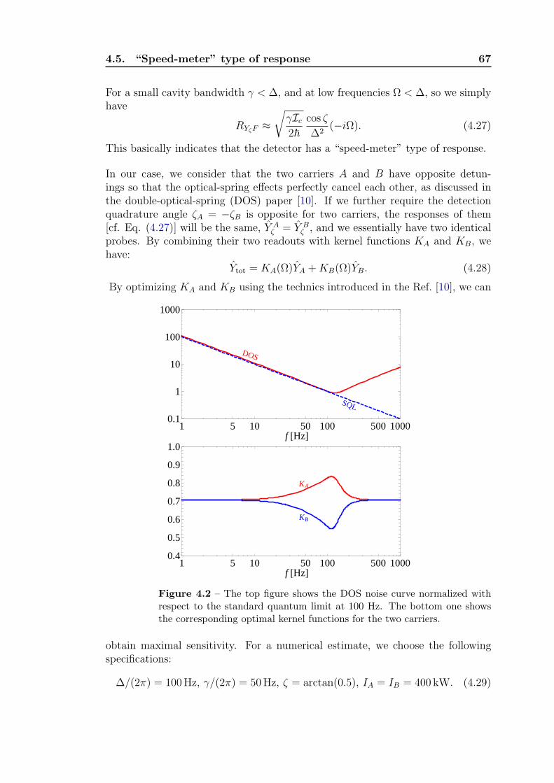
4.5. “Speed-meter” type of response 67
For a small cavity bandwidth γ < ∆, and at low frequencies Ω < ∆, so we simplyhave
RYζF ≈√γIc
2~cos ζ
∆2(−iΩ). (4.27)
This basically indicates that the detector has a “speed-meter” type of response.
In our case, we consider that the two carriers A and B have opposite detun-ings so that the optical-spring effects perfectly cancel each other, as discussed inthe double-optical-spring (DOS) paper [10]. If we further require the detectionquadrature angle ζA = −ζB is opposite for two carriers, the responses of them[cf. Eq. (4.27)] will be the same, Y A
ζ = Y Bζ , and we essentially have two identical
probes. By combining their two readouts with kernel functions KA and KB, wehave:
Ytot = KA(Ω)YA +KB(Ω)YB. (4.28)
By optimizing KA and KB using the technics introduced in the Ref. [10], we can
1 5 10 50 100 500 10000.1
1
10
100
1000
f @HzD
SQL
DOS
1 5 10 50 100 500 10000.4
0.5
0.6
0.7
0.8
0.9
1.0
f @HzD
KA
KB
Figure 4.2 – The top figure shows the DOS noise curve normalized withrespect to the standard quantum limit at 100 Hz. The bottom one showsthe corresponding optimal kernel functions for the two carriers.
obtain maximal sensitivity. For a numerical estimate, we choose the followingspecifications:
∆/(2π) = 100Hz, γ/(2π) = 50Hz, ζ = arctan(0.5), IA = IB = 400 kW. (4.29)

68Chapter 4. Modifying Test-Mass Dynamics: Double Optical Spring
The resulting noise curve and the optimal kernel functions are shown in Fig. 4.2.At low frequencies, we almost follow the SQL. There is actually an analyticalformula for the noise curve, which is:
Sh(Ω) =1
L2
[1
|RYζF |2+S2SQL(Ω)
4|RYζF |2
]≥ Sh
SQL, (4.30)
where SSQL = ~/(mΩ2) and the optical power is twice that of an individual carrier.Given the response in Eq. (4.27), we have:
Sh(Ω) = ShSQL
[1
|RYζF |2SSQL
+SSQL(Ω)
4|RYζF |2
]∝ Sh
SQL. (4.31)
Thiss basically means that we can follow the SQL but never be able to surpass it.This is in contrast with a true “speed meter” in which the SQL can be surpassedsignificant as long as we have a sufficient large optical power. The next questionwould be how we could recover the true “speed-meter” response in the DOSconfiguration.
4.6 Conclusions and future work
We have shown the possibility of a “negative inertia” effect attributable to thespecific frequency dependence of double optical springs. This is capable of re-ducing the effective inertia of the probe mass, and thus can significantly enhancethe mechanical response of the interferometer to GW signals. This effect the in-terferometer to surpass the free-mass SQL over a wide frequency band. Thereare several issues that need to be further investigated: (i) the stability of thesystem. What feedback control method is necessary to stabilize the system? (cf.the discussions in Ref. [63] for the single optical spring case); (ii) if one uses athird carrier for readout purposes, how much improvement in sensitivity couldbe obtained, compared to the current double-carrier case? In addition, we haveconsidered the “speed-meter” type of response, and have shown that a doubleoptical spring allows us to follow the SQL at low frequencies.

Chapter 5
Measuring a Conserved Quantity:Variational Quadrature Readout
5.1 Preface
In this chapter, we consider surpassing the Standard Quantum Limit(SQL) for measuring a weak force with a mechanical oscillator. By usinga time-dependent variational readout, we can measure the mechanicalquadrature—a conserved quantity of the oscillator motion—and evademeasurement-induced back-action. This is motivated by the pioneeringwork of Vyatchanin et al. [17, 18], in which such a back-action-evadingvariational scheme is proposed to detect a force signal with known arrivaltime. Here, we will go beyond such a limitation and make it suitable forall possible stationary signals, which can be characterized by their spec-trum. This will be useful for: (i) improving the sensitivity of future GWdetectors if the test-mass frequency (∼1 Hz) is upshifted to the detec-tion band (∼ 100 Hz) by the optical-spring effect and (ii) improving thesensitivity of an atom force microscopy with a high-frequency mechani-cal oscillator as the probe. This is a continuing joint research effort byStefan Danilishin, Yanbei Chen, and myself.
5.2 Introduction
Due to recent significant achievements in fabricating high-quality mechanical de-vices, electromechanical and optomechanical devices have played important rolesin probing weak forces and tiny displacements. Two notable examples on thelarge scale and small scale are: (i) a gravitational-wave detector, in which kg-scale test-masses are coupled to high-power optical field for probing tiny ripplesin the spacetime—gravitational waves [72], and (ii) an atomic-force microscope,in which a micromechanical oscillator coupled to an electric or optical field is usedto probe atomic forces [1]. Their force sensitivity is limited by the SQL [74], and
70Chapter 5. Measuring a Conserved Quantity: Variational Quadrature
Readout
which has a spectral density of:
SSQLF (Ω) =
~|Rxx(Ω)|
, (5.1)
where the mechanical response Rxx(Ω) = −1/m[(Ω2 − ω2m)] for a high-Q oscillator
with eigenfrequency ωm. The origin of such a limit comes from the fact that we tryto measure the external force by monitoring the changes in the oscillator positionx at different times, which do not commute with each other, i.e.,
[x(t), x(t′)] = − i~mωm
sinωm(t− t′). (5.2)
This leads to the following Heisenberg uncertainty principle:
∆x(t)∆x(t′) ≥ ~2mωm
sinωm(t− t′), (5.3)
which basically means that the oscillator positions at different times cannot besimultaneously measured with an arbitrarily high accuracy; this gives rise to theSQL for the force sensitivity.
There are two approaches to overcoming such a limit [74]: (i) a stroboscopicmeasurement. Thiss measures the oscillator with pulses separated by an integertimes the oscillation period. From the commutator relation Eq. (5.2), we learnthat if t − t′ = 2nπ/ωm, [x(t), x(t′)] = 0, and, then they are simultaneouslymeasurable; (ii) as quadrature measurement. Instead of measuring the oscillatorposition, this measures quantum nondemolition (QND) observables—mechanicalquadratures X1,2 which are defined through the equation:
x(t) ≡ X1(t) cosωmt+X2(t)
mωm
sinωmt. (5.4)
These observables satisfy
[X1(t), X1(t′)] = [X2(t), X2(t
′)] = 0, [X1(t), X2(t′)] = i~δ(t− t′). (5.5)
Therefore, if we are able to detect the force by measuring only one of the quadra-tures, e.g., X1(t), there will not be an associated quantum limit. To realize such ameasurement, Braginsky et al. proposed to modulate the electro/optomechanicalinteraction strength G at the mechanical frequency, namely G(t) = G0 cosωmt[16]. Specifically, the interaction Hamiltonian can be written as:
Hint = ~G(t)x(t)a1(t) = ~G0 cosωmt
[X1(t) cosωmt+
X2(t)
mωm
sinωmt
]a1(t)
=1
2~G0
[X1(t) + X1(t) cos 2ωmt+
X2(t)
mωm
sin 2ωmt
], (5.6)

5.3. Dynamics 71
where a1(t) represents the electrical/optical degrees of freedom. If a1(t) is changingslowly compared with 2ωm and it does not have a significant fluctuation at 2ωm,we will measure the QND observable X1 without imposing any back-action. Foroptomechanical devices, this can be realized with a mechanical oscillator coupledto a high-finesse cavity, such that the cavity bandwidth γ is much smaller thanthe mechanical frequency, as proposed by Clerk et al. [92].
Here, we will consider another regime where the probing field is not slowly chang-ing and has fluctuations at 2ωm, e.g., one with a large cavity bandwidth in thecase of a cavity-assisted scheme. With a time-domain variational readout, we canevade the measurement-induced back-action from the output data, thus realizinga quasi-QND measurement. This will be useful for small-scale atomic force mi-croscopy, where a high-finesse cavity could be difficult to incorporate. It is alsouseful for large-scale GW detectors, because a large cavity bandwidth is preferredfor increasing the detection bandwidth.
The outline of this chapter is as follows: In Sec. 5.3, we will analyze the dynamicsof an optomechanical system. In Sec. 5.4, we will consider the time-domain vari-ational scheme and demonstrate how the back action can be evaded if effectivelysense only one of the quadrature. One limitation for such a scheme is that it losethe resonant gain. In Sec. 5.5, we will introduce another variational scheme whichmimics a stroboscopic measurement, in which we can recover the resonant gainby introducing an insignificant back-action.
5.3 Dynamics
Figure 5.1 – A schematic plot showing an optomechanical system. Amechanical oscillator with eigenfrequency ωm interacts with a cavity modea, which is also coupled to the input (ain) and output (aout) optical modes.
A schematic plot of a typical cavity-assisted optomechanical device is shown inFig. 5.1. In the limit of a large cavity bandwidth γ ≫ ωm, with the cavity modeadiabatically eliminated, the input-output relation for the optical field becomes,
b1(t) = a1(t), (5.7)
b2(t) = a2(t) + (α/~)x(t). (5.8)

72Chapter 5. Measuring a Conserved Quantity: Variational Quadrature
Readout
Here a1,2 (b1,2) are the input (output) amplitude and phase quadratures; α de-termines the interaction strength, and it is related to the optical power I0 byα ≡ 8
√2(F/λ)
√~I0/ω0 where F is the cavity finesse, and ω0 the laser frequency.
The equations of motion for the oscillator are
˙x(t) = p(t)/m, (5.9)
˙p(t) = −mω2mx(t) + α a1(t) + ξth(t). (5.10)
Here, we can split the oscillator position into a perturbed part δx, and a freeoscillation part xq, which is given by:
xq(t) = δxq[X0 cosωmt+ P0 sinωmt], (5.11)
where δxq ≡√~/(2mωm). The perturbed part includes the effects of the radiation-
pressure noise, thermal noise, and external driving force (our signal), namely:
δx(t) =∫ t
0dt′Gx(t− t′)[α a1(t
′) + ξth(t′) + Fext(t
′)], (5.12)
where Gx(t) ≡ Θ(t) sinωmt/(mωm) denotes the Green’s function.
5.4 Variational quadrature readout
In order to make the detection scheme work for all possible signals, we need todiscretize the measurement process into small time sections, the sum of which tellsus the shape of the signal. This idea is similar to the discrete sampling variationalmeasurement discussed in Ref. [93, 94], in which a back-action-evading schemefor a free mass is proposed. Here, we try to derive the noise spectrum for thisscheme, and focus on the oscillator case.
Suppose we divide the measurement from t = 0 to t = T into N sections (thespectral resolution bandwidth is given by 1/T ). For simplicity, we assume thateach section has the same duration ∆τ , namely ∆τ = T/N . With time-dependenthomodyne detection, we can construct the following N integral estimators for theoutput signal:
Yi =∫ τi+1
τidt[g(i)1 (t)b1(t) + g
(i)2 (t)b2(t)
], (τi = i∆τ, i = 0, 1, · · · , N−1). (5.13)
In order to form a quasi-QND measurement, each section should measure thesame quadrature. This is because:
[Yi, Yj] = 0 (i = j), [Xζ , Xζ′ ] = 0. (5.14)
That is, different quadratures are probed, the added noise between different sec-tions will be Heisenberg-limited. This condition can be trivially satisfied if τ

5.4. Variational quadrature readout 73
is equal to an integer times the oscillation period, and g2 is the correspondingperiodic function. One simple choice would be:
∆τ = τm = 2π/ωm, g(j)2 (t) = g
(i)2 (t+ j τm − i τm). (5.15)
In this case, the filtering function has the following Fourier decomposition:
g2(t) =1
τm
+∞∑n=−∞
g2,n(nωm) e−i n ωmt, g2,n(nωm) =
∫ τm0dt g2(t) e
i n ωmt. (5.16)
We encounter one immediate problem with this scheme: each section only sensesa1 for one oscillation period, while the effects of back-action accumulate fromt = 0. The back-action of each section can not be evaded, if the filtering functionsonly satisfy the back-action-evading (BAE) condition (cf. Eq. (5.18). As it turnsout, we have to sacrifice the sensitivity around the mechanical resonance. Thisis because of the following argument: by swapping the integration order, theback-action part of the estimator:
δYi =∫ τi+1
τidt g
(i)1 (t)a1(t) + (α2/~)
∫ τi+1
τidt a1(t)
∫ τi+1
tdt′Gx(t
′ − t) g(i)2 (t′)
+ (α2/~)∫ τi0dt a1(t)
∫ τi+1
τidt′Gx(t
′ − t) g(i)2 (t′). (5.17)
If the BAE condition is satisfied, namely:
g(i)1 (t) + (α2/~)
∫ τi+1
tdt′Gx(t
′ − t) g(i)2 (t′) = 0. (5.18)
We haveδYi = (α2/~)
∫ τi0dt a1(t)
∫ τi+1
τidt′Gx(t
′ − t) g(i)2 (t′). (5.19)
Therefore, to eliminate this accumulated back-action, we require∫ τi+1
τidt′Gx(t
′ −t) g
(i)2 (t′) = 0 for any t, which automatically leads to:∫ τi+1
τidt g
(i)2 (t)xq(t) = 0. (5.20)
If this is the case, we obtain:
Y BAEi =
∫ τi+1
τidt g
(i)2 (t)[a2(t) + (α/~)
∫ t
τidt′Gx(t− t′)Fext(t
′)]. (5.21)
We can recover the sensitivity around ωm by using stroboscopic variation mea-surement, as we will discuss in Sec. 5.5. Even though we do not have resonancegain, this scheme could still be interesting if the signals that we are searching fordo not have frequency components at ωm.
In the following, we will derive the noise spectrum for such a scheme. Using theseBAE estimators, we can construct the output spectrum for the entire measurementprocess; we have:
Zn = τm
N−1∑k=0
Y BAEk ei n ωeτk , ωe ≡ 2π/T. (5.22)

74Chapter 5. Measuring a Conserved Quantity: Variational Quadrature
Readout
The corresponding spectrum SZZ would be defined through
⟨ZnZn′⟩ = SZZ δnn′Nτm. (5.23)
Substituting the expressions for g2 and Y BAEk into the above equation, and after
some straightforward calculations, we obtain:
SZZ(nωe) =∞∑
k=−∞
|gk(k ωm)|2[1
2+α2
~24 sin2(nωeτm/2)
(nωeτm + 2kπ)2R2
xx(nωe)SF (nωe)
](gk(±ωm) = 0), (5.24)
where the mechanical response function Rxx(ω) = [m(ω2 − ω2m)]
−1. Taking thelimit T → ∞ (i.e., a very good bandwidth resolution), we have:
SZZ(Ω) =∞∑
k=−∞
|gk(k ωm)|2[1
2+α2
~2sin2(ω τm/2)
[(ω τm/2) + k π]2R2
xx(Ω)SF (Ω)
], (5.25)
where q is the squeezing factor—a 10 dB squeezing gives e−2q = 0.1; SF (Ω) is theforce noise spectrum that contains both thermal noise, and the external drivingforce. This result is intuitively expected. Basically, the displacement sensitivityis the original one multiplied by the sinc function due to the discrete sampling.Therefore, if the GW signal has a characteristic frequency much lower than themechanical frequency, the filtering function g2 should be mostly a constant. Inthis case, the normalized noise is given by:
Sh(Ω) =1
m2L2Ω4
[~2
2α2
(Ω τm/2)2
sin2(Ω τm/2)R−2
xx (Ω) + SthF (Ω)
]. (5.26)
Even though this is shot-noise limited, this sensitivity does not really increasea lot at low frequencies, because it rises as 1/Ω2 and physically we know thatthe oscillator does not has a good response at low frequencies. However, we showthat back-action can be evaded simply by manipulating the output, for all possiblesignal.
5.5 Stroboscopic variational measurement
In order to recover the sensitivity around the mechanical resonance, we haveto devote most of the measurement time to the amplitude quadrature, and onlymeasure the phase quadrature for a short period of time ∆t≪ ω−1
m every oscillatorcycle — the idea of stroboscopic variational measurement. This is different fromwhat is proposed in Ref. [93] and here the driving field is still constant in time.
As in previous considerations, we divide the measurement into N sections with∆τ = τm. Instead of measuring both amplitude and phase quadrature simulta-neously, we measure the phase quadrature during [τi, τi +∆t], and switch to the

5.5. Stroboscopic variational measurement 75
amplitude quadrature during [τi+∆t, τi+1]. Mathematically, we have the following2N integral estimators:
Xi =∫ τi+1
τi+∆tdt g
(i)1 (t) b1(t), Yi =
∫ τi+∆t
τidt g
(i)2 (t) b2(t). (5.27)
To minimize the back-action, we can construct the following quantities:
Oi ≡i−1∑n=0
Xn(t) + Yi(t). (5.28)
Basically, for each phase quadrature readout, we take into account all the back-action imposed during the history. One can easily find that as long as g1(t) andg2(t) are periodic functions at the mechanical frequency and
g(i)1 (t) +
∫ τi+∆t
τidt′Gx(t
′ − t)g(i)2 (t′) = 0, (t < τi) (5.29)
we have
Oi =∫ τi+∆t
τidt g
(i)2 (t)a2(t) + (α/~)g(i)2 (t)
∫ t
0dt′Gx(t− t′)[αH(t′)a1(t
′) + Fext(t)],(5.30)
where H(t) is a periodic function of τm and H(t) = Θ(t) − Θ(t − ∆t) during[0, τm]. Therefore, most of the back actions are evaded, and the remaining partis imposed during the period when we measure the phase quadrature. This isexactly the same as in the stroboscopic measurement, but with an importantdifference that the probing light beam is always on in our case, which is morefeasible experimentally. By applying the same procedure as in the previous case,we can evaluate the output spectrum from:
Zn = τm
N−1∑k=1
(Ok − O0) ei n ωeτk . (5.31)
Here we remove the initial condition term of the oscillator position by subtractingOk with O0. After some manipulations, and expanding the results in series ofωm∆t, we find:
SZZ(nωe) =∞∑
k=−∞
|gk(k ωm)|2∆t
2τm+
N0∑k=−N0
|gk(k ωm)|2[
α4∆t5
24 ~2m2τm sin2(nωeτm/2)+α2∆t2
2~2τ 2mR2
xx(nωe)SF (nωe)
],
(5.32)
where N0 ωm∆t ≪ 1 so that the Taylor expansion is justified, and terms withlarger k are small and do not contribute to the summation. Suppose g2 only has afrequency component at ωm. Taking the continuous limit, the normalized spectraldensity for detecting GWs is given by:
Sh(Ω) =1
m2L2Ω4
[~2τm
α2R2xx(Ω)∆t
+α2τm∆t
3
12m2R2xx(Ω) sin
2(Ω τm/2)+ Sth
F (Ω)
]. (5.33)

76Chapter 5. Measuring a Conserved Quantity: Variational Quadrature
Readout
Due to the presence of the sin factor in the denominator, the back-action noisenever vanishes, even at the mechanical resonance. However, the added noise inprinciple can be arbitrarily small, if the optimal time scale is chosen, and themeasurement is sufficiently sensitive.
5.6 Conclusions
We have considered two types of variational measurement schemes for measuringthe QND variable—the mechanical quadrature. In both cases, there are insignif-icant contributions from the back action-noise to the sensitivity. In contrast tothe approach of modulating the interaction strength, and requiring a good-cavitycondition, we have considered the case with a large cavity bandwidth. There-fore, these schemes are more suitable for small-scale cavity-assisted devices andlarge-scale broadband GW detectors.

Chapter 6
MQM with Three-ModeOptomechanical Interactions
6.1 Preface
In this chapter, we discuss the Macroscopic Quantum Mechanics (MQM)of a three-mode optomechanical system, in which two orthogonal trans-verse optical cavity modes are coupled to one mechanical mode throughradiation pressure. This work is motivated by the investigations of three-mode parametric instability in large-scale gravitational-wave (GW) de-tectors with high-power optical cavities, as first pointed out by Braginskyet al. [95]. We realized that the same mechanism that induces instability,in a different parameter regime, can also be used to cool the mechanicalresonator down to its quantum ground state. Different from the classicalanalysis by Braginsky et al., we present a full quantum analysis of three-mode optomechanical parametric interactions, which properly takes intoaccount quantum fluctuations and correlations. We obtain the quantumlimit for the ground state cooling with three-mode interactions. In addi-tion, we show that it can also create tripartite optomechanical quantumentanglement between the cavity modes and the mechanical oscillator.Compared with the conventional cavity-assisted optomechanical devicesusing a single cavity mode, three-mode interactions can achieve an op-timal frequency matching: the frequency separation of the two cavitymodes is equal to the mechanical-mode frequency. This allows the carrierand sideband fields to simultaneously resonate and coherently build up.Such a mechanism significantly enhances the optomechanical couplingsin the quantum regime. It allows us to explore quantum behaviors of op-tomechanical interactions in small-scale table-top experiments. We showexplicitly that given experimentally achievable parameters, three-modescheme can realize quantum ground-state cooling of milligram scale me-chanical oscillators and create robust stationary tripartite optomechan-ical quantum entanglements. This chapter summarizes a joint researcheffort by Chunnong Zhao, Li Ju, David Blair, Zhongyang Zhang and me.The relevant publications are Phys. Rev. A 78, 063809 (2008), Phys.Rev. A 79, 063801 (2009), andu Phys. Rev. Letts. 104, 243902 (2009).

78 Chapter 6. MQM with Three-Mode Optomechanical Interactions
6.2 Introduction
Optomechanical interactions have recently become of great interest, for their po-tential in exploring the quantum behavior of macroscopic objects. Various experi-ments have demonstrated that the mechanical mode of a mechanical oscillator canbe cooled significantly through two-mode optomechanical interactions [9, 19, 21–28, 31, 32, 34]. The basic setup consists of a Fabry-Perot cavity with an endmirror. Linear oscillations of the mirror mechanical mode at frequency ωm scatterthe optical-cavity mode (usually TEM00) at frequency ω0 into Stokes (ω0 − ωm)and anti-Stokes (ω0 + ωm) sideband modes, which have the same spatial modeshape as the TEM00 mode. The optical cavity is appropriately detuned such thatthe anti-Stokes sideband is close to resonance. Therefore, the anti-Stokes processis favored over the Stokes process. As a natural consequence of energy conserva-tion, the thermal energy of the mechanical mode has to decrease in order to createhigher-energy anti-Stokes photons at ω0+ωm. If the cavity-mode decay rate, whichis related to the optical finesse, is smaller than the mechanical-mode frequency,theoretical analysis shows that these experiments can eventually achieve the quan-tum ground state of a macroscopic mechanical oscillator [44, 45, 96], which wouldbe a significant breakthrough in physics from both experimental and theoreticalpoints of view. With the same scheme, many interesting issues have been raisedin the literature, such as teleportation of a quantum state into mechanical degreesof freedom [97], creation of stationary quantum entanglements between the cav-ity mode and the mechanical oscillator [51, 98], or even between two oscillators[53, 54]. This in turn could be implemented in future quantum communicationsand computing.
The concept of three-mode optomechanical parametric interactions was first in-troduced and analyzed theoretically in the pioneering work of Braginsky et al.[95]. It was shown that three-mode interactions inside high-power optical cavitiesof large-scale laser interferometric gravitational-wave (GW) detectors have thepotential to induce instabilities, which would severely undermine the operationof detectors. This analysis was elaborated by many other authors to more accu-rately simulate the real situation in next-generation advanced gravitational-wavedetectors [99–102] and to find strategies for suppressing instability [103, 104]. Re-cently, the UWA group experimentally demonstrated three-mode interactions inan 80-m high-power optical cavity by exciting the mechanical modes and observingresonant scattering of light into a transverse cavity mode [105].
In contrast to the two-mode case, in three-mode interactions, a single mechani-cal mode of the mechanical oscillator scatters the main cavity TEM00 mode intoanother transverse cavity mode, which has a different spatial distribution fromthe TEM00 mode. Specifically, when the TEM00 mode is scattered by the me-chanical mode, the frequency is split into Stokes and anti-Stokes sidebands atω0 ±ωm, and in addition, the spatial wavefront is also modulated by the mechan-

6.2. Introduction 79
ical mode. Three-mode interactions strongly arise when both the modulationfrequency and spatial mode distribution are closely matched to those of anothertransverse optical-cavity mode. Under these circumstances, both the carrier andsideband modes are simultaneously resonant inside the cavity and get coherentlybuild up. Taking into account the resonance of the mechanical mode, the systemis triply resonant, with the interaction strength scaled by the product of the twooptical quality factors and the mechanical quality factor. If the transverse opticalcavity mode has a frequency lower than the TEM00 mode, the Stokes sidebandwill be on resonance and the interaction provides positive amplification of themechanical mode, while if the transverse mode has a frequency above the maincavity TEM00 mode, the anti-Stokes sideband will resonate, and the system hasnegative gain and the mechanical mode will be cooled. The underlying principleof both two and three mode interactions is similar to the Brillouin scattering,except that the modulation occurs not through changes in refractive index of themedium, but through bulk surface motion of a macroscopic mechanical oscillator(i.e. the mechanical mode) which modulates the optical path of the light.
While three-mode interactions are inconvenient by-products of the design of ad-vanced GW detectors, they can be engineered to occur in small-scale systemswith low mass resonators, which can serve as an optomechanical amplifier and beapplied to mechanical-mode cooling [106, 107]. Besides, due to its triply resonantfeature, the three-mode system has significant advantages compared with the two-mode system and allows much stronger optomechanical couplings. To motivateexperimental realizations, we have suggested a small-scale table-top experimentwith a milligram mechanical oscillator in a coupled cavity [107]. Using the extradegree of freedom of the coupled cavity, the cavity mode gap (i.e., the differencebetween the two relevant cavity modes) can be continuously tuned such that itis equal to plus or minus the mechanical-mode frequency, which maximizes thethree-mode interaction strength. We also pointed out that, in the negative-gainregime, this experimental setup can be applied to resolved-sideband cooling of amechanical oscillator down to its quantum ground state. In that paper, we usedthe classical analysis presented by Braginsky et al. to obtain the effective thermaloccupation number n of the mechanical mode. This analysis breaks down whenn ≪ 1 and the quantum fluctuations of the cavity modes have to be taken intoaccount. To overcome this limitation, we used the similarity in the Hamiltonianof the two-mode and the three-mode system, and argued that the quantum limitfor cooling in both systems is the same without investigating the detailed dynam-ics. However, in order to gain a quantitative understanding of the three-modesystem in the quantum regime, it is essential to develop a full quantum analysiswhich includes the dynamical effects of the quantum fluctuations. Besides, as wewill show, the quantum analysis reveals a most interesting non-classical feature ofthree-mode systems: stationary tripartite quantum entanglement.
The outline of this chapter is as follows: in Sec. 6.3, we start from the classi-cal analysis given by Braginsky et al. and then quantize it with the standard

80 Chapter 6. MQM with Three-Mode Optomechanical Interactions
approach. In Sec. 6.4, we use the quantized Hamiltonian as the starting pointto analyze the dynamics of the three-mode system. Further, based upon theFluctuation-Dissipation-Theorem (FDT), we derive the quantum limit for theachievable thermal occupation number in cooling experiments. To motivate futuresmall-scale experiments, we provide an experimentally achievable specification forthe quantum ground state cooling of a mechanical oscillator. In Sec. 6.5, we in-vestigate the stationary tripartite optomechanical quantum entanglement, and weshow that the same specification for the cooling experiments can also be appliedto realize robust stationary optomechanical entanglements.
6.3 Quantization of three-mode parametric in-
teractions
In this section, we will first present the classical formulations of three-mode op-tomechanical parametric interactions given by Braginsky et al. [95], and thenapply standard procedures to obtain the quantized version.
Classical Picture. A detailed quantitative classical formulation of three-modeinteractions was given in the Appendix of Ref. [95]. A Lagrangian formalism wasused to derive the classical equations of motion and analyze the stability of theentire three-mode optomechanical system. The formalism can be easily convertedinto Hamiltonian language, which can then be quantized straightforwardly. Forconvenience, we will use slightly different notation and definitions for the opticalfields. Further, we assume that the two optical-cavity modes are the TEM00
and TEM01 modes, and that the mechanical mode has a torsional mode shape(about the vertical axis) which has a large spatial overlap with the TEM01 modeas shown in Fig. 6.1. This can be easily extended to general cases with othertransverse optical modes and mechanical modes. Assuming the electric field islinearly polarized in the transverse direction perpendicular to the z axis, theelectromagnetic fields (E,H) of the cavity modes can be written as:
Ei(t) =
(~ωi
ϵ0V
)1/2
fi(r⊥) sin(kiz)qi(t), (6.1)
Hi(t) =ϵ0ki
(~ωi
ϵ0V
)1/2
fi(r⊥) cos(kiz)qi(t). (6.2)
Here, i = 0, 1 represent the TEM00 and TEM01 modes; fi(r⊥) are the transversemode shapes; ωi denotes the eigenfrequency; ki are the wave numbers; V is thevolume of the optical cavity; qi(t) are the generalized coordinates of the fields;and qi(t) are the time derivatives of qi(t). At the present stage, the appearanceof ~ωi is just to make the generalized coordinates qi dimensionless. The classical
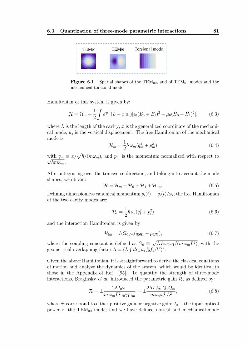
6.3. Quantization of three-mode parametric interactions 81
TEM00 TEM01 Torsional modeTEM00 TEM01
Figure 6.1 – Spatial shapes of the TEM00, and of TEM01 modes and themechanical torsional mode.
Hamiltonian of this system is given by:
H = Hm +1
2
∫dr⊥(L+ xuz)[ϵ0(E0 + E1)
2 + µ0(H0 +H1)2], (6.3)
where L is the length of the cavity; x is the generalized coordinate of the mechani-cal mode; uz is the vertical displacement. The free Hamiltonian of the mechanicalmode is
Hm =1
2~ωm(q
2m + p2m) (6.4)
with qm ≡ x/√
~/(mωm), and pm is the momentum normalized with respect to√~mωm.
After integrating over the transverse direction, and taking into account the modeshapes, we obtain:
H = Hm +H0 +H1 +Hint. (6.5)
Defining dimensionless canonical momentum pi(t) ≡ qi(t)/ωi, the free Hamiltonianof the two cavity modes are:
Hi =1
2~ωi(q
2i + p2i ) (6.6)
and the interaction Hamiltonian is given by
Hint = ~G0qm(q0q1 + p0p1), (6.7)
where the coupling constant is defined as G0 ≡√Λ ~ω0ω1/(mωmL2), with the
geometrical overlapping factor Λ ≡ (L∫dr⊥uzf0f1/V )2.
Given the above Hamiltonian, it is straightforward to derive the classical equationsof motion and analyze the dynamics of the system, which would be identical tothose in the Appendix of Ref. [95]. To quantify the strength of three-modeinteractions, Braginsky et al. introduced the parametric gain R, as defined by:
R = ± 2ΛI0ω1
mωmL2γ0γ1γm= ±2ΛI0Q0Q1Qm
mω0ω2mL
2, (6.8)
where ± correspond to either positive gain or negative gain; I0 is the input opticalpower of the TEM00 mode; and we have defined optical and mechanical-mode

82 Chapter 6. MQM with Three-Mode Optomechanical Interactions
quality factors Qi = ωi/γi (i = 0, 1,m). Due to optomechanical interaction, thedecay rate γm of the mechanical mode will be modified to an effective one γ′m,which is
γ′m ≈ (1−R)γm. (6.9)
When R > 1, the decay rate becomes negative and this corresponds to instability.In this paper, we are particularly interested in the regime whereR < 0 which givesrise to the mechanical-mode cooling. The effective thermal occupation numbern′th of the mechanical mode is given by
n′th =
nthγmγ′m
=nth
1−R(6.10)
with nth denoting the original thermal occupation number. It seems that when−R ≫ 1, n′
th can be arbitrarily small. However, in this case, the classical analysisbreaks down and the quantum fluctuations of the cavity modes will set forth aquantum limit for the minimally achievable n′
th, which will be detailed in thefollowing quantum analysis.
Quantized Hamiltonian. The classical Hamiltonian derived above can be quantizedby identifying the generalized coordinate and momentum as Heisenberg operators,which satisfy the following commutation relations:
[qj, pj′ ] = i δjj′ , (j, j′ = 0, 1,m). (6.11)
The quantized Hamiltonian is then given by
H =1
2
∑i=m,0,1
~ωi(q2i + p2i ) + ~G0qm(q0q1 + p0p1) + Hext, (6.12)
where we have added Hext to take into account the coupling between cavity modesand external continuum optical fields due to the non-zero transmission of the cav-ity. This Hamiltonian is convenient for discussing stationary tripartite quantumentanglement as will be shown in Sec. 6.5, as these generalized coordinates qiand pi correspond to the amplitude and phase quadratures in the quantum opticsentanglement experiments.
To discuss the ground-state cooling as will be investigated in Sec. 6.4, it is il-luminating to introduce annihilation operators for the two cavity modes a ≡(q0 + i p0)/
√2 and b ≡ (q1 + i p1)/
√2, so that the normally-ordered quantized
Hamiltonian can be rewritten as:
H =1
2~ωm(q
2m + p2m) + ~ω0a
†a+ ~ω1b†b+ ~G0qm(a
†b+ b†a) + Hext. (6.13)

6.4. Quantum limit for three-mode cooling 83
6.4 Quantum limit for three-mode cooling
In this section, we will start from the Hamiltonian in Eq. (6.13) to derive thedynamics and discuss the quantum limit for the ground-state cooling experimentsusing three-mode optomechanical interactions. As we will see, due to similarmathematical structure as in the two-mode case, the corresponding quantum limitfor three-mode cooling is identical to the resolved-sideband limit derived by Mar-quardt et al. [44] and Wilson-Rae et al. [45] in the two-mode case.
Equations of Motion. The dynamics of this three-mode system can be derivedfrom the quantum Langevin equations (QLEs). In the experiments, the TEM00
mode is driven on resonance at ω0. Therefore, we choose a rotating frame at ω0,obtaining the corresponding nonlinear QLEs as:
˙qm = ωmpm, (6.14)
˙pm = −ωmqm − γmpm −G0(a†b+ b†a) + ξth, (6.15)
˙a = −γ0 a− i G0qmb+√2γ0 ain, (6.16)
˙b = −(γ1 − i∆)b− i G0qma+
√2γ1 bin. (6.17)
Here the TEM00 and TEM01 mode gap is given by ∆ ≡ ω1 − ω0; G0(a†b + b†a)
corresponds to the radiation pressure which modifies the dynamics of the mechan-ical mode and is also responsible for the quantum limit; we have added thermalnoise ξth whose correlation function, in the Markovian approximation, is given by⟨ξth(t)ξth(t′)⟩ = 2γmnthδ(t − t′). In obtaining the above equations, we have alsoused the Markovian approximation for Hext, namely:
Hext = i ~(√2γ0 a
†ain +√2γ1 b
†bin −H.c.) (6.18)
with H.c. denoting the Hermitian conjugate.
To solve the above equations, we can linearize them by replacing every Heisen-berg operator with the sum of a steady part and a small perturbed part, namelyo = o + δo(ϵ) with ϵ ≪ 1. We treat the Brownian thermal noise ξth, the vacuumfluctuations
√γ0δain,
√γ1δbin and δqm as being of the order of ϵ. In the experi-
ments, the TEM00 mode is pumped externally with a large classical amplitude ainwhile the TEM01 mode is not with bin = 0. Therefore, to the zeroth order of ϵ,the steady part of the cavity modes are simply given by
a =√
2/γ0 ain =√2I0/(γ0~ω0), b = −iG0aqm. (6.19)
Without loss of generality, we can set qm = 0. Therefore, b = 0 and this allows usto eliminate the TEM00 mode from the first-order equations, which are:
δ ˙qm = ωm δpm, (6.20)
δ ˙pm = −ωm δqm − γm δpm −G0a(δb+ δb†) + ξth, (6.21)
δ˙b = −(γ1 + i∆)δb− i G0a δqm +
√2γ1 δbin. (6.22)

84 Chapter 6. MQM with Three-Mode Optomechanical Interactions
Here we have chosen an appropriate phase reference such that ain is real andpositive. The above equations can be solved in the frequency domain, namely:
qm(Ω) = −ωm[Frp(Ω) + ξth(Ω)]
(Ω2 − ω2m) + i γmΩ
, (6.23)
δb(Ω) =G0 a δqm(Ω) + i
√2γ1δbin(Ω)
(Ω−∆) + i γ1, (6.24)
where the radiation pressure
Frp(Ω) =2G2
0 a2∆ δqm(Ω)− 2G0a
√γ1[(γ1 − iΩ)δq2(Ω)−∆ δp2(Ω)]
[(Ω−∆) + i γ1][(Ω + ∆) + i γ1](6.25)
with the amplitude and phase quadratures δq2(Ω) = [δb(Ω) + δb†(−Ω)]/√2 and
δp2(Ω) = [δb(Ω)−δb†(−Ω)]/(√2i). In the expression for Frp, the part proportional
to δqm is due to the optical spring effect. For a high quality-factor oscillator withωm ≫ γm, the decay rate γm and the eigenfrequency ωm of the mechanical modewill be modified to new effective values γ′m and ω′
m, as given by:
γ′m = γm +4G2
0 a2∆ωmγ1
[(ωm −∆)2 + γ21 ][(ωm +∆)2 + γ21 ], (6.26)
ω′m = ωm +
G20a
2∆(ω2m −∆2 − γ21)
[(ωm −∆)2 + γ21 ][(ωm +∆)2 + γ21 ]. (6.27)
In our case, the TEM00 and TEM01 mode gap is ∆ = ω1 − ω0 = ωm. In theresolved-sideband case with γ1 ≪ ωm, we obtain:
γ′m ≈ γm +G2
0a2
γ1; ω′
m ≈ ωm − G20a
2
4ωm
. (6.28)
If we define the parametric gain as R = (γm − γ′m)/γm, then in this case
R = −G20a
2
γ1γm= − 2ΛI0ω1
mωmL2γ0γ1γm. (6.29)
This is identical to Eq. (6.8) in the negative-gain regime, which was obtained fromclassical analysis by Braginsky et al. [95]. However, in contrast to Eq. (6.10), theresulting thermal occupation number of the mechanical mode is given by
n′th =
nthγmγ′m
+ nquant =nth
1−R+ nquant (6.30)
where the extra term nquant originates from the vacuum fluctuations in Frp, i.e.terms proportional to δp2 and δq2. Since, in the case of large R, or equivalentlystrong optomechanical coupling, n′
th ≈ nquant and the mechanical mode will finallyreach a thermal equilibrium with the cavity modes. The lowest achievable thermaloccupation number nquant will be determined by this optical heat bath (i.e., cavitymode + external continuum mode).

6.4. Quantum limit for three-mode cooling 85
To derive this quantum limit nquant, we will apply the Fluctuation-Dissipation-
Theorem (FDT). Specifically, given any two quantities A(t) and B(t) which lin-early depend on field strength, we can define the forward correlation function:
CAB(t− t′) ≡ ⟨A(t)B(t′)⟩ (t > t′), (6.31)
where ⟨ ⟩ denotes the ensemble average. According to the FDT, we have
SAB(Ω) + SAB(−Ω)
SAB(Ω)− SAB(−Ω)=eβ ~Ω + 1
eβ ~Ω − 1= 2neff(Ω) + 1, (6.32)
or equivalently,
neff(Ω) =SAB(−Ω)
SAB(Ω)− SAB(−Ω). (6.33)
where SAB(Ω) is the power spectral density (Fourier transform of CAB), β =1/(kBTeff) and the effective thermal occupation number neff ≡ 1/(eβ ~Ω − 1). Inour case, we can simply substitute A,B with the amplitude of the TEM01 mode δbby fixing qm = 0. From Eq. (6.24) and using the fact that for vacuum fluctuation⟨δbin(Ω)δb†in(Ω′)⟩ = 2πδ(Ω− Ω′), we obtain:
Sδb δb(Ω) =2γ1
(Ω−∆)2 + γ21. (6.34)
Since the mechanical mode have a very high intrinsic quality factor (ωm ≫ γm),the energy transfer between the cavity modes and the mechanical mode onlyhappens around ωm. Therefore, from Eq. (6.33) and Eq. (6.34), the final quantumlimit is given by:
nquant ≈ neff(ωm) =
(γ12ωm
)2
, (6.35)
where we have used the fact that for the resonant case, ∆ = ω1 − ω0 = ωm. Toachieve the quantum ground state, i.e. nquant ∼ 0, we require ωm ≫ γ1 and this issimply the resolved-sideband limit obtained in the pioneering works of Marquardtet al. [44] and Wilson-Rae et al. [45].
The reason why the quantum limit for three-mode cooling is identical to the two-mode case can be readily understood from the fact that the TEM00 mode is elim-inated from the optomechanical dynamics as shown explicitly in Eq. (6.20)(6.21)(6.22) and we essentially obtain an effective two-mode system. As suggested byYanbei Chen [private communication], this equivalence can be made more obviousby mapping this three-mode system into a power and signal-recycled laser inter-ferometer, as shown in Fig. 6.2. The TEM00 and TEM01 modes can be viewedas the common and differential modes in the interferometer, respectively. Thetorsional mode corresponds to the differential motion of the end mirrors and ∆is equivalent to the detuning of the signal-recycling cavity. In the power- andsignal-recycled interferometer, even though there is no high-order transverse op-tical mode involved, the two degrees of freedom of the power-recycling mirror

86 Chapter 6. MQM with Three-Mode Optomechanical Interactions
Figure 6.2 – Equivalent mapping from a three-mode system to a power-and signal-recycled interferometer. The TEM00 and TEM01 modes can beviewed as the common and differential optical modes in the interferometerrespectively. The torsional mechanical mode is equivalent to the differentialmotion of two end mirrors in the interferometer. By adjusting the positionsof the power-recycling mirror (PRM) and signal-recycling mirror (SRM),we can make the carrier and sideband modes simultaneously resonate insidethe cavity, the same as in the three-mode scheme.
and the signal recycling mirror enable simultaneous resonances of the carrier andsideband modes, which is achieved naturally with the three-mode optomechanicalscheme.
The above discussion shows that, mathematically, two-mode interactions andthree-mode interactions are very similar. However, it is very important to empha-size that, from an experimental point of view, there is an important difference.Specifically, the steady-state amplitude a in the radiation pressure Frp is amplifiedby the optical resonance, while for the two-mode case, this amplitude is highlysuppressed due to large detuning. In other words, in order to achieve the sameoptomechanical coupling strength experimentally, the input optical power in thetwo-mode scheme needs to be 1 + (∆/γ0)
2 times larger than the the three-modescheme. This is a large factor in the resolved-sideband regime with ∆ ≫ γ0 (theoptimal ∆ = ωm). Besides, in the three-mode interactions, the condition ∆ = ωm
also naturally optimizes the energy transfer from the mechanical mode to the cav-ity mode [44, 45, 108]. Therefore, the three-mode scheme greatly enhances theoptomechanical coupling and is able to achieve resolved-sideband limit withoutcompromising the intra-cavity optical power. As mentioned in Ref. [106], the am-plitude and laser phase noise can also be reduced significantly with three-modescheme, simply due to the filtering of the cavity resonance.
To motivate future cooling experiments with three-mode interactions, we nowpresent an experimentally achievable specification for the quantum ground statecooling of a milligram-scale mechanical oscillator. We choose that the mass ofthe mechanical oscillator m = 0.1mg; the length of the cavity L = 2 cm; themechanical-mode frequency ωm/2π = 106 Hz; the mechanical-mode quality factorQm ≡ ωm/γm = 107; and the optical finesse F = 104. Given an input optical

6.5. Stationary tripartite optomechanical quantum entanglement 87
power of the TEM00 mode I0 = 50mW, and the environmental temperatureT = 4K, the corresponding effective thermal occupation number of the mechanicaloscillator ∼ 0.5.
6.5 Stationary tripartite optomechanical quan-
tum entanglement
As shown in the works of Vitali et al. [51] and Paternostro et al. [98], optome-chanical interaction provides a very efficient way of generating stationary quantumentanglements among cavity modes and the mechanical mode. Once experimen-tally realized, it will have significant impact on future quantum communications.Following their formalism, we will investigate the stationary tripartite quantumentanglement in the three-mode optomechanical system by first analyzing thedynamics and then evaluating the entanglement measure —the logarithmic nega-tivity EN defined in Refs. [109, 110].
Starting from the Hamiltonian in Eq. (6.12), the corresponding nonlinear QLEsin the rotating frame at the laser frequency ωL can be written as:
˙qm = ωmpm, (6.36)
˙pm = −ωmqm − γmpm −G0(q0q1 + p0p1) + ξth, (6.37)
˙q0 = −γ0q0 +∆0p0 +G0qmp1 +√
2γ0qin0 , (6.38)
˙p0 = −γ0p0 −∆0q0 −G0qmq1 +√
2γ0 pin0 , (6.39)
˙q1 = −γ1q1 +∆1p1 +G0qmp0 +√
2γ1qin1 , (6.40)
˙p1 = −γ1p1 −∆1q1 −G0qmq0 +√
2γ1 pin1 , (6.41)
where ∆0 = ω0−ωL, and ∆1 = ω1−ωL. Slightly different from the cooling experi-ments, here we need to externally drive both the TEM00 and TEM01 modes simul-taneously, to create tripartite quantum entanglement. We choose an appropriatephase reference such that the classical amplitude pi = 0 and qi = 0 (i = 0, 1),which is related to the input optical power Ii by qi =
√2Ii/(~ωiγi). Similar to
the previous case, we can linearize the above equations as:
˙xT = MxT + nT, (6.42)
with T denoting the transpose:
xT ≡ ( δqm, δpm, δq0, δp0, δq1, δp1 )T, (6.43)
nT ≡ ( 0, ξth,√2γ0 δq
in0 ,
√2γ0 δp
in0 ,
√2γ1 δq
in1 ,
√2γ1 δp
in1 )T, (6.44)

88 Chapter 6. MQM with Three-Mode Optomechanical Interactions
and matrix M is given by:
M =
0 ωm 0 0 0 0
−ωm −γm G0q1 0 G0q0 00 0 −γ0 ∆0 0 0
G0q1 0 −∆0 −γ0 0 00 0 0 0 −γ1 ∆1
G0q0 0 0 0 −∆1 −γ1
. (6.45)
At first sight, this mathematical structure is identical to the one analyzed byPaternostro et al. [98]. Apart from differing in the coupling constants (here weneed to consider the overlapping factor Λ), there is another important difference:after linearization, the radiation pressure term G0(q0q1 + p0p1) in Eq. (6.37) isproportional to q0δq1 + q1δq0, rather than to q0q0 − q1q1, as considered in Ref.[98]. As we will show, similar to the case for cooling experiments, the coherentbuild-up of both the TEM00 and TEM01 modes, and the optimal mode gap ω1 −ω0 = ωm enhance the entanglement significantly, which make it easier to achieveexperimentally.
Assuming the system is stable, i.e., all eigenvalues of M have negative real parts,the stationary solutions to Eq. (6.42) can be written formally as:
xi(∞) =∑j
∫ ∞
0
dt′[eM(t−t′)]ijnj(t′), (6.46)
where we have neglected the initial-condition terms, which decay away as the sys-tem approaches the stationary state. We assume that all the noises are MarkovianGaussian processes, and that the correlation functions are:
σij(t− t′) ≡ Dij δ(t− t′), (6.47)
where Dij are the elements of matrix D, and
Dij = Diag[0, 2γmkBT/(~ωm), γ0, γ0, γ1, γ1]. (6.48)
The corresponding stationary covariance matrix among the cavity modes and themechanical mode can then be written as:
V(∞) =
∫ ∞
0
dt[eMt]D[eMt]T, (6.49)
and the components ofV can be obtained by solving the following linear equations:
MV +VMT = −D. (6.50)
For this tripartite continuous-variable system (one mechanical mode + two cavitymodes), one necessary and sufficient condition for separability is the positivity of

6.5. Stationary tripartite optomechanical quantum entanglement 89
partially-transposed covariance matrix [111–113]. In our case, a partial transposeis equivalent to time reversal and can be realized by reversing the momentum ofthe mechanical mode from pm to −pm, namely
Vpt = V|pm→−pm . (6.51)
By evaluating the positivity of the eigenvalue of Vpt, we can directly determinewhether entanglement exists or not. To reveal the richness of the entanglementstructure, we will not directly analyze the positivity of Vpt for the entire system,but rather, following Ref. [98], we look at the entanglement between any bipartitesubsystem using the logarithmic negativity EN . Given the 4×4 covariance matrixVsub for any bipartite subsystem,
Vsub =
[A2×2 C2×2
CT2×2 B2×2
], (6.52)
the logarithmic negativity EN is defined by [110, 111]
EN = max[0,− ln 2σ−] (6.53)
with σ− ≡√Σ−
√Σ2 − 4 detVsub/
√2, and Σ ≡ detA+ detB− 2 detC.
For numerical estimations, we will use the same specification as given in the pre-vious section for the cooling experiments. We will focus on the situation relevantto the experiments, with ω1−ω0 = ωm, and the TEM00 mode driven on resonance(∆0 = 0, ∆1 = ωm). In Fig. 6.3, we show the resulting EN as a function of theinput optical powers of both optical modes. Given the specifications, the entan-glement strength between each optical mode and the mechanical mode becomesstronger as the optical power of their counterpart increases (until the system be-comes unstable). This is understandable, because we have a qm(q0q1 + q0q1) typeof interaction, and the coupling strength between the TEM00 mode and the me-chanical mode directly depends on the classical amplitude of the TEM01 and viceversa. For the entanglement between the two optical modes, this reaches a maxi-mum when both modes have medium power. This can be attributable to the factthat the entanglement between these two optical modes is mediated by the me-chanical mode, and both E0m
N and E1mN should be large to give a reasonable E01
N .Besides, as shown explicitly in Fig. 6.4, the condition ω1−ω0 = ωm will naturallyoptimize the entanglement between the TEM01 mode and the mechanical mode.This is because the Lorentzian profiles of the TEM01 mode and the mechanicalhave the largest overlap when ∆ = ωm. In this case, both the TEM01 mode andthe mechanical mode are driven by the same vacuum field, which gives the max-imal entanglement. Therefore, the optimal condition for the cooling experimentwill simultaneously optimize the entanglement strength, as has also been observedby Genes et al. [108].
To illustrate the robustness of this tripartite entanglement, we show the depen-dence of EN on the environmental temperature in Fig. 6.5. The entanglement

90 Chapter 6. MQM with Three-Mode Optomechanical Interactions
0.020.04
0.06
0.080.1
0.130.15
0.17 0.19
0 1 2 3 4 5 6 70.0
0.2
0.4
0.6
0.8
I0 HWL
I1HWL
0.04
0.080.12 0.17 0.21
0.25
0.30.34
0.38
0 1 2 3 4 5 6 70.0
0.2
0.4
0.6
0.8
I0 HWL
I1HWL
0.003
0.006
0.009
0.012
0 1 2 3 4 5 6 70.0
0.2
0.4
0.6
0.8
I0 HWL
I1HWL
Figure 6.3 – Logrithmic negativity EN as a function of the input opticalpowers of both modes. Other specifications are identical to those for coolingexperiments given in the previous section. The left panel shows E0m
N for theentanglement between the TEM00 mode and the mechanical mode; Themiddle panel presents E1m
N for the TEM01 mode and the mechanical mode;the right panel shows E01
N for the TEM00 mode and the TEM01 mode.
Figure 6.4 – Logarithmic negativity E1mN as a function of the cavity modes
gap ∆ ≡ ω1 − ω0. As we can see, the condition ∆ ≈ ωm, which optimizesthe cooling, also maximizes the entanglement between the TEM01 modeand the mechanical mode. Here we have assumed I0 = 4.5W (higher I0will make the system unstable for small ∆) and I1 = 0.W. Since it can beviewed as an effective two-mode system in this case with I1 = 0, we simplyrecover the results given by Vitali et al. [51].
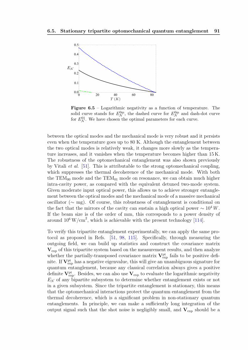
6.5. Stationary tripartite optomechanical quantum entanglement 91
Figure 6.5 – Logarithmic negativity as a function of temperature. Thesolid curve stands for E0m
N , the dashed curve for E0mN and dash-dot curve
for E01N . We have chosen the optimal parameters for each curve.
between the optical modes and the mechanical mode is very robust and it persistseven when the temperature goes up to 80 K. Although the entanglement betweenthe two optical modes is relatively weak, it changes more slowly as the tempera-ture increases, and it vanishes when the temperature becomes higher than 15K.The robustness of the optomechanical entanglement was also shown previouslyby Vitali et al. [51]. This is attributable to the strong optomechanical coupling,which suppresses the thermal decoherence of the mechanical mode. With boththe TEM00 mode and the TEM01 mode on resonance, we can obtain much higherintra-cavity power, as compared with the equivalent detuned two-mode system.Given moderate input optical power, this allows us to achieve stronger entangle-ment between the optical modes and the mechanical mode of a massive mechanicaloscillator (∼ mg). Of course, this robustness of entanglement is conditional onthe fact that the mirrors of the cavity can sustain a high optical power ∼ 104W .If the beam size is of the order of mm, this corresponds to a power density ofaround 106 W/cm2, which is achievable with the present technology [114].
To verify this tripartite entanglement experimentally, we can apply the same pro-tocol as proposed in Refs. [51, 98, 115]. Specifically, through measuring theoutgoing field, we can build up statistics and construct the covariance matrixVexp of this tripartite system based on the measurement results, and then analyzewhether the partially-transposed covariance matrix Vpt
exp fails to be positive defi-nite. If Vpt
exp has a negative eigenvalue, this will give an unambiguous signature forquantum entanglement, because any classical correlation always gives a positivedefinite Vpt
exp. Besides, we can also use Vexp to evaluate the logarithmic negativityEN of any bipartite subsystem to determine whether entanglement exists or notin a given subsystem. Since the tripartite entanglement is stationary, this meansthat the optomechanical interactions protect the quantum entanglement from thethermal decoherence, which is a significant problem in non-stationary quantumentanglements. In principle, we can make a sufficiently long integration of theoutput signal such that the shot noise is negligibly small, and Vexp should be a

92 Chapter 6. MQM with Three-Mode Optomechanical Interactions
direct verification of what we have obtained theoretically.
6.6 Three-mode interactions with a coupled cav-
ity
Figure 6.6 – The optical modes of a single Fabry-Perot cavity with length∼ 10 cm. The panel (a) shows the mode distribution for a near-concentriccavity with g-factor ∼ −1 which is suitable for observing PI, while panel (b)is the near-planar case with g-factor ∼ 1 which suits for cooling experiment.In both cases, there are no symmetric modes on the opposite side of theTEM00 mode because the higher-order mode TEMmn marked with ‘?’ arehighly lossy due to diffraction losses. This is preferred for experimentalrealizations of three-mode interactions because we know from Eq. (6.8)that any symmetric mode on the opposite side of the TEM00 mode willreduce the absolute value of the parametric gain. However, both cavitiesare marginally stable and very susceptible to misalignment.
In this section, we will discuss how to explore three-mode interactions using acoupled cavity. To make our analysis close to realistic experiments, we considera torsional acoustic mode with frequency ∼ 1 MHz interacting with the opticalTEM10 and TEM00 modes. This configuration is chosen because MHz frequencycan be easily achieved in a mm-scale structure, and the torsional mode has a largespatial overlap with the TEM10 mode.
To begin with, let us consider a single Fabry-Perot cavity to see why a coupled
M0 M1 M2
Ein
Eout
E01
E10
E01eidf01/2
E10e-idf01/2
E12
E21
E12eidf12/2
E21e-idf12/2
+ - + - - +
M0 M1 M2
+ - + - - +r0t0
r1t1
r2t2
Figure 6.7 – The optical fields of the coupled cavity. Here δϕ01,12 arethe round-trip phase shifts of light in the sub-cavity (formed by M0 andM1), and in the main cavity (formed by M1 and M2), respectively. We usethe convention that the mirrors have minus reflectivity on the side with acoating layer.

6.6. Three-mode interactions with a coupled cavity 93
cavity is necessary. The free spectral range of a single cavity with length ∼ 10 cmis approximately 1 GHz. Therefore, as shown in Fig. 6.6, one has to build either anear-planar or near-concentric cavity to obtain a desired mode gap around 1 MHzbetween the TEM10 and TEM00 modes. For both cases, the cavity is marginallystable and susceptible to misalignment. It is also difficult to get accesses to bothinstability and cooling regimes in a single setup. Creating a coupled Fabry-Perotcavity solves these problems. As we will show later, the resulting scheme is stable.Additionally, we can easily tune between the instability and cooling regimes. Thecoupled cavity is showed schematically in Fig. 6.7. It is similar to the configurationof power- or signal-recycling interferometers [8, 62] when one considers either thecommon mode or the differential mode. The field dynamics can be easily obtainedas shown in Ref. [116], by treating the sub-cavity as an effective mirror, withfrequency- and mode-dependent transmissivity and reflectivity. Specifically, theeffective transmissivity t01 is:
t01 ≡E12
Ein
=t0t1
1 + r0r1eiδϕ01, (6.54)
and the effective reflectivity r10 is given by:
r10 ≡E12
E21
= −r1 −t21r0e
iδϕ01
1 + r0r1eiδϕ01. (6.55)
The corresponding E12 inside the main cavity can be written as:
E12 =Eint01
1 + r10r2eiδϕ12=
Eint011− |r10|r2ei[arg(r10)+δϕ12+π]
. (6.56)
The resonance occurs when the phase factor in Eq. (6.56) is equal to 2nπ,which critically depends upon the phase angle of the effective reflectivity, namelyarg(r10). Specifically, when the TEM00 mode resonates inside the main cavity,which requires that δϕTEM00
01 = δϕTEM0012 = 2nπ, the phase shift of the TEM10
mode δϕTEM10ij is:
δϕTEM10ij =
2Lij
c∆ω − 2Φij
g + 2n′π, ij = 01, 12, (6.57)
where ∆ω ≡ ω1 − ω0 is the mode gap between TEM10 and TEM00; Φg is theGouy phase and n, n′ are integers. In order to satisfy the resonant conditionfor three-mode interactions, we need to adjust δϕTEM10
01 , which changes arg(r10),such that ∆ω = ±ωm. To achieve this, one obvious way is to change the lengthof sub-cavity L01, but this turns out to be impractical due to a small tuningrange. An alternative and more practical approach, as shown in Fig. 6.8, is toadd another lens or concave mirror inside the sub-cavity to tune the Gouy phaseΦ01
g . The resulting scheme is similar to the proposed stable recycling cavity fornext-generation gravitational-wave detectors [117]. With the additional lens, theGaussian beam gets focused inside the sub-cavity. Since the Gouy phase changes

94 Chapter 6. MQM with Three-Mode Optomechanical Interactions
M0 L1 M2M1Tuning
L01 L12
Laser & mode-
matching optics
Tuning
Figure 6.8 – The optical layout for the table top experiment, where a 1MHz torsional micro-oscillator (M2) interacts with the optical TEM10 modeand the TEM00 mode. By tuning the positions of mirror M0 and lens L1, wecan continuously change the frequency of TEM10. If the losses in L1 werean issue, it could easily be replaced by a concave mirror.
from almost −π2to π
2within one Rayleigh range around the waist, one can easily
obtain a desired δϕTEM1001 simply by adjusting the position of M0 near the waist.
This might lead to problems with power density due to the small waist size, butfor the table top experiment we consider here, the power density is quite low.
The corresponding Φ01g with an additional lens can be derived straightforwardly
by using the ray transfer relation for a Gaussian beam, which is given by
q′ =fq
f − q. (6.58)
Here f is the focal length of L1; q(′) ≡ z(
′) + iz(′)R ; z is the displacement relative to
the waist; zR is the Rayleigh range and superscript ′ denotes quantities after thelens. This dictates
z′ =f(zf − z2 − z2R)
(f − z)2 + z2R, (6.59)
z′R =zRf
2
(f − z)2 + z2R. (6.60)
The resulting Gouy phase at any point is given by
Φg(z) =
arctan (z/zR) , z < zLarctan [(z − zL + z′L)/z
′R] + arctan (zL/zR)− arctan (z′L/z
′R) , z ≥ zL
(6.61)
where z(′)L is the position of L1 relative to the waist. Gouy phase Φ01
g is thedifference between wavefront at M0 and M1, namely
Φ01g = Φg(zM0)− Φg(zM1), (6.62)
where zM0 and zM1 are the positions of M0 and M1 relative to the waist respectively.Therefore, by adjusting the positions of M0 and L1 as shown in Fig. 6.8, we cancontinuously tune Φ01
g such that ∆ω = ωm.
Equations (6.54) to (6.62) provide the design tools of the coupled cavity for three-mode interactions. To realize the experiment, we first need to design the main

6.6. Three-mode interactions with a coupled cavity 95
M0 L1 M2M1(a) Mode matching for Stokes mode (R>0)
236 mm 74 mm 75 mm
M0 L1 M2M1
(b) Mode matching for Anti-Stokes mode (R<0)
232 mm 77 mm 75 mm
Figure 6.9 – The mode matching for the positive gain and negative gainby adjusting the relative position of M0 and L1. Only small adjustment isneeded to tune from one case to another.
Cooling
Instability
Po
sitio
n of
M0 r
elat
ive
to L
1 [m
m]
(a)
Frequency difference between TEM10 and TEM00 [Hz]
(b)
Cooling
Frequency difference between TEM10 and TEM00 [Hz]
Posi
tion
of L
1 re
lativ
e to
M1 [
mm
]
Instability
Figure 6.10 – Panels (a) and (b) show the mode gap between TEM10
and TEM00 as a function of position of M0 relative to L1 and position ofL1 relative to M1 respectively. The dots in both figures are the situationsconsidered in Fig. 6.9. Clearly, we can tune between the instability andcooling regimes continuously.
cavity and specify L12, ωm, the radius of curvatures (RoCs) of M0,M1,M2 and thefocal length of L1. From Eq. (6.56) and Eq. (6.57), we can find out the requiredarg(r01) which gives the right mode gap between TEM10 and TEM00. This willgives us one constraint. Combining with the requirement of mode matching toM0, we can fix two degrees of freedom of the system, namely the positions of M0
and L1. To demonstrate this principle explicitly, we present a solution that isclose to a realistic experimental setup. We assume the following:
L12 = 75 mm ωm = 1MHz f = 100 mm,
R0 = 500 mm r0 =√0.999 A0 = 500 ppm,
R1 = 100 mm r1 =√0.9 A1 = 500 ppm,
R2 = ∞ mm r2 =√0.9995 A2 = 500 ppm.
Here, Ri(i = 0, 1, 2) are RoCs; ri denotes the amplitude reflectivity; ti is theamplitude transmissivity and Ai is the optical loss which satisfy r2i + t2i + Ai =1 (i = 0, 1, 2).
The results of mode matching for both positive- (instability) and negative-gain(cooling) configurations are shown in Fig. 6.9. In Fig. 6.10, we show the modegap between TEM10 and TEM00 as a function of the position of M0 relative toL1 and the position of L1 relative to M1. In this particular case, the dependenceis almost linear with a slope ∼ 2mm/MHz for both panels. This indicates that
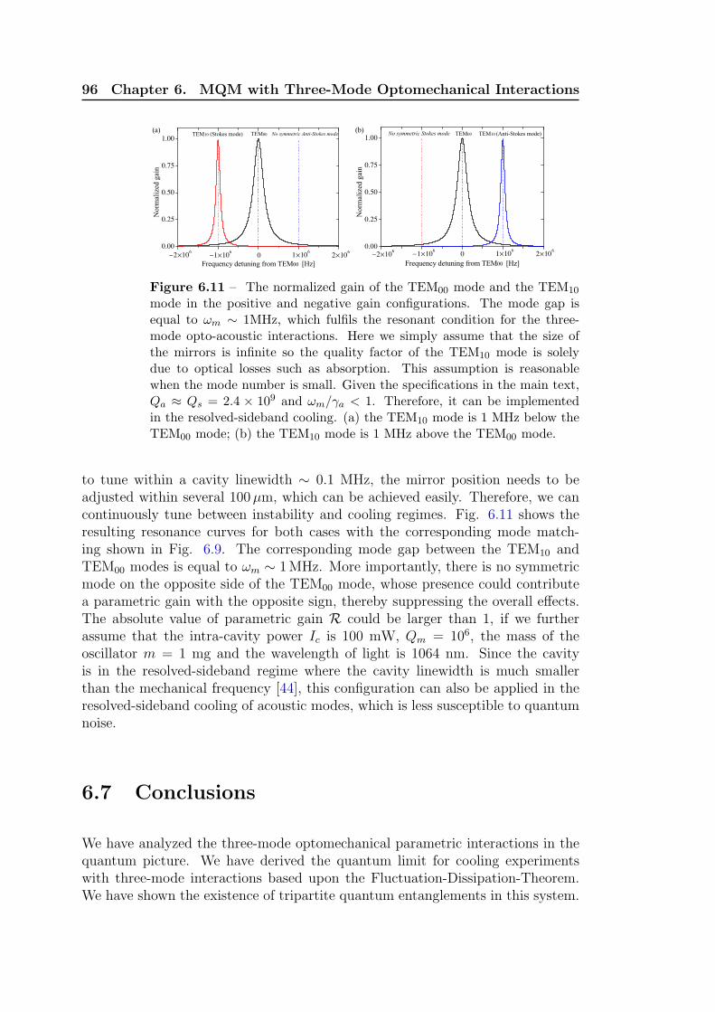
96 Chapter 6. MQM with Three-Mode Optomechanical Interactions
(a) TEM00 No symmetric Anti-Stokes mode
Nor
mal
ized
gai
n
Frequency detuning from TEM00 [Hz]
TEM10 (Stokes mode) No symmetric Stokes mode TEM00 TEM10 (Anti-Stokes mode)
Nor
mal
ized
gai
n
Frequency detuning from TEM00 [Hz]
(b)
Figure 6.11 – The normalized gain of the TEM00 mode and the TEM10
mode in the positive and negative gain configurations. The mode gap isequal to ωm ∼ 1MHz, which fulfils the resonant condition for the three-mode opto-acoustic interactions. Here we simply assume that the size ofthe mirrors is infinite so the quality factor of the TEM10 mode is solelydue to optical losses such as absorption. This assumption is reasonablewhen the mode number is small. Given the specifications in the main text,Qa ≈ Qs = 2.4 × 10⁹ and ωm/γa < 1. Therefore, it can be implementedin the resolved-sideband cooling. (a) the TEM10 mode is 1 MHz below theTEM00 mode; (b) the TEM10 mode is 1 MHz above the TEM00 mode.
to tune within a cavity linewidth ∼ 0.1 MHz, the mirror position needs to beadjusted within several 100µm, which can be achieved easily. Therefore, we cancontinuously tune between instability and cooling regimes. Fig. 6.11 shows theresulting resonance curves for both cases with the corresponding mode match-ing shown in Fig. 6.9. The corresponding mode gap between the TEM10 andTEM00 modes is equal to ωm ∼ 1MHz. More importantly, there is no symmetricmode on the opposite side of the TEM00 mode, whose presence could contributea parametric gain with the opposite sign, thereby suppressing the overall effects.The absolute value of parametric gain R could be larger than 1, if we furtherassume that the intra-cavity power Ic is 100 mW, Qm = 106, the mass of theoscillator m = 1 mg and the wavelength of light is 1064 nm. Since the cavityis in the resolved-sideband regime where the cavity linewidth is much smallerthan the mechanical frequency [44], this configuration can also be applied in theresolved-sideband cooling of acoustic modes, which is less susceptible to quantumnoise.
6.7 Conclusions
We have analyzed the three-mode optomechanical parametric interactions in thequantum picture. We have derived the quantum limit for cooling experimentswith three-mode interactions based upon the Fluctuation-Dissipation-Theorem.We have shown the existence of tripartite quantum entanglements in this system.

6.7. Conclusions 97
The simultaneous resonances of the carrier and sideband modes in the three-modesystem allows more efficient mechanical-mode cooling and more robust optome-chanical entanglement than in the two-mode system. This work provides thetheoretical basis for the feasibility of realizing both ground-state cooling and sta-tionary optomechanical quantum entanglements using three-mode optomechanicalparametric interactions in small-scale table-top experiments and also large-scaleGW interferometers.


Chapter 7
Achieving the Ground State andEnhancing OptomechanicalEntanglement
7.1 Preface
In the previous chapter, we have seen that in order to achieve the quan-tum ground state of a mechanical oscillator, with three-mode or evengeneral optomechanical devices, the cavity bandwidth needs to be smallerthan the mechanical frequency. This is the so-called resolved-sideband orgood-cavity limit. In this chapter, we provide a new but physically equiv-alent insight into the origin of such a limit: that is information loss due toa finite cavity bandwidth. With an optimal feedback control to recoverthis information, we can surpass the resolved-sideband limit and achievethe quantum ground state. Interestingly, recovering this information canalso significantly enhance the optomechanical entanglement. Especiallywhen the environmental temperature is high, the entanglement will ei-ther exist or vanish, depending critically on whether the information isrecovered or not, which is a vivid example of a quantum eraser. This is ajoint research effort by Stefan Danilishin, Helge Muller-Ebhardt, YanbeiChen, and myself. This is available on line at arXiv:1003.4048.
7.2 Introduction
Recently, achieving the quantum ground state of a macroscopic mechanical oscil-lator has aroused great interest among physicists. It will not only have significantimpact on quantum-limited measurements [74] but will also shed light on quantumentanglements involving macroscopic mechanical degrees of freedom [50–54, 98],which can be useful for future quantum computing and help us to understandtransitions between the classical and quantum domains [118–121].
By using conventional cryogenic refrigeration, O’Connell et al. have successfully

100Chapter 7. Achieving the Ground State and Enhancing
Optomechanical Entanglement
cooled a 6 GHz micromechanical oscillator down to its ground state [122]. Mean-while, in order to cool larger-size and lower-frequency mechanical oscillators athigh environmental temperature, there have been great efforts in trying differentapproaches: active feedback control, and parametrically coupling the oscillator tooptical or electrical degrees of freedom [9, 19–37, 123]. The cooling mechanism hasbeen extensively discussed, and certain classical and quantum limits have beenderived [43–45, 106, 108, 124–127]. In the case of cavity-assisted cooling schemes,pioneering theoretical works by Marquardt et al. [44] and Wilson-Rae et al. [45]showed that the quantum limit for the occupation number is (γ/2ωm)
2 1. Thisdictates that, in order to achieve the ground state of the mechanical oscillator,the cavity bandwidth γ must be smaller than the mechanical frequency ωm, whichis the so-called “resolved-sideband” or “good-cavity” limit. This limit is derivedby analyzing the quantum fluctuations of the radiation pressure force on the me-chanical oscillator. From a physically equivalent perspective, it can actually beattributable to information loss: information of the oscillator motion leaks intothe environment without being carefully treated, which induces decoherence.
This perspective immediately illuminates two possible approaches for surpassingsuch a limit: (i) the first one is to implement the novel scheme proposed by Elste etal. [128], in which the quantum noise is destructively interfered, and informationof the oscillator motion around ωm does not leak into the environment. Corbittsuggested an intuitive understanding by thinking of an optical cavity with a mov-able front mirror rather than a movable end mirror in those cooling experiments[private communication]. In this hypothetical scheme, the optical fields directlyreflected, and those filtered through the cavity, both contain the information ofthe front-mirror motion. If the cavity detuning is appropriate, these two piecesof information destructively interfere with each other, and the quantum coher-ence of the mechanical oscillator is maintained. (ii) the second approach is torecover the information by detecting the cavity output. This will work because aconditional quantum state—the best knowledge of the oscillator state, conditionalon the measurement result—is always pure for an ideal continuous measurementwith no readout loss. Indeed, when the cavity bandwidth is much larger thanthe mechanical frequency, the cavity mode will follow the oscillator dynamics andcan therefore be adiabatically eliminated. The quantum noise can be treatedas being Markovian and a standard Stochastic-Master-Equation (SME) analysishas already shown how the conditional quantum state approaches a pure stateunder a continuous measurement [38–42]. For the non-zero cavity bandwidthconsidered here, the cavity mode has a dynamical timescale comparable to thatof the mechanical oscillator. Correspondingly, the quantum noise has correlationsat different times, and is non-Markovian. To estimate the conditional state, aWiener-filtering approach is more transparent than the SME [129]. As we willshow, the conditional quantum state of the oscillator in the cavity-assisted cool-
1There is a factor of two difference in defining the cavity bandwidth here compared with theone defined in Ref. [44].

7.2. Introduction 101
ing schemes is indeed almost pure, with a residual impurity contributed by thethermal noise, and by imperfections in detections and optomechanical entangle-ment between the oscillator and the cavity mode. In order to further localize theoscillator in phase space and achieve its ground state, an optimal feedback controlis essential [43]. In Fig. 7.1, the final occupation number of the unconditionalstate and optimally controlled state is shown. As long as the optimal control isapplied, the minimally achievable occupation number of the oscillator will not beconstrained by the resolved-sideband limit.
0.050.1
0.30.6
1.02.0
4.0
9.0
-2.0 -1.5 -1.0 -0.5 0.00.10.51.01.52.02.53.0
DΩm
ΓΩ
m
0.009
0.0140.02
0.03 0.04
0.060.08
-2.0 -1.5 -1.0 -0.5 0.00.10.51.01.52.02.53.0
DΩmΓΩ
m
Figure 7.1 – A contour plot of the occupation number as a function ofcavity bandwidth γ and detuning ∆ for the unconditional state (left) asobtained in Refs. [44, 45] and optimally controlled state (right), for whichthe details are in Secs. 7.4, 7.5, 7.6.
Another interesting issue in the optomechanical system is creating a quantumentanglement between the cavity mode and the oscillator, or even between twooscillators [51, 53, 54, 98, 125, 130]. Intuitively, one might think that such anentanglement must be very vulnerable to thermal decoherence, and that the envi-ronmental temperature needs to be extremely low in order to create it. However,as shown in Ref. [54], and in a more recent investigation [131], the environmentaltemperature—even though being an important factor—affects the entanglementimplicitly, and only the ratio between the interaction strength and thermal de-coherence matters. The reason why, in Refs. [51, 53, 98, 125], the temperatureplays a dominant role in determining the existence of the entanglement can alsobe traced back to information loss, as briefly mentioned in Ref. [131]. Here, wewill address this issue more explicitly. Fig. 7.2 shows that by recovering the in-formation contained in the cavity output, the optomechanical entanglement caneven be revived at high temperature. This is a vivid example of a quantum eraserfirst proposed by Scully and Druhl [132] and later demonstrated experimentally[133]: quantum coherence can be revived by recovering lost information.
The outline of this chapter is as follows: in Sec. 7.3, we will analyze the systemdynamics by applying the standard Langevin-equation approach and derive thespectral densities of important dynamical quantities. In Sec. 7.4, we obtain un-conditional variances of the oscillator position and momentum, and evaluate thecorresponding occupation number, which recovers the resolved-sideband limit. In

102Chapter 7. Achieving the Ground State and Enhancing
Optomechanical Entanglement
Recovering information
Without recovering information
Figure 7.2 – Optomechanical entanglement strength EN as a function oftemperature T with (solid) and without (dashed) recovering information(details are in Sec. 7.7).
Sec. 7.5, conditional variances are derived via the Wiener-filtering approach, whichclearly demonstrates that the conditional quantum state is almost pure. In Sec.7.6, we show the occupation number of the optimally controlled state and thecorresponding optimal controller to achieve it. In Sec. 7.7, we consider the op-tomechanical entanglement and demonstrate that significant enhancements in theentanglement strength can be achieved after recovering information. In Sec. 7.8, tomotivate cavity-assisted cooling experiments, we consider imperfections in a realexperiment and obtain a numerical estimation of the occupation number givena set of experimentally achievable specifications. Finally, we conclude with ourmain results in Sec. 7.9.
7.3 Dynamics and Spectral Densities
Figure 7.3 – Schematic plot of an optomechanical system with a mechanicaloscillator x coupled to a cavity mode a, which in turn couples to the externalingoing (ain) and outgoing (aout) optical field.
In this section, we will analyze the optomechanical dynamics and derive the spec-tral densities of relevant quantities which are essential for calculating the occupa-tion number of the mechanical oscillator.

7.3. Dynamics and Spectral Densities 103
7.3.1 Dynamics
Even though the dynamics of such a system has been discussed extensively in theliterature [44, 45, 108], we will go through some equations for the coherence ofthis article. An optomechanical system and the relevant dynamical quantities areshown schematically in Fig. 7.3. The corresponding Hamiltonian is given by:
H = ~ωc a†a+
p2
2m+
1
2mω2
mx2 + ~G0x a
†a+ i ~√
2γ (aine−i ω0 ta† −H.c.). (7.1)
Here, ωc and ω0 are the cavity resonant frequency and the laser frequency, respec-tively; a is the annihilation operator for the cavity mode, which satisfies [a, a†] = 1;x and p denote the oscillator position and momentum, with [x, p] = i ~; m is themass of the oscillator; G0 ≡ ω0/L is the optomechanical coupling constant, withL the cavity length. In the rotating frame at the laser frequency ω0, a set ofnonlinear Langevin equations can be obtained:
˙x(t) = p(t)/m, (7.2)
˙p(t) = −γmp(t)−mω2mx(t)− ~G0a
†(t)a(t) + ξth(t), (7.3)
˙a(t) = −(γ − i∆)a(t)− i G0x(t)a(t) +√
2γ ain(t), (7.4)
where the cavity detuning ∆ ≡ ω0 − ωc. To take into account the fluctuation-dissipation mechanism of the oscillator coupled to a thermal heat bath at tempera-ture T , we have included the mechanical damping γm and the associated Brownianforce ξth, of which the correlation function is ⟨ξth(t)ξth(t′)⟩ = 2mγmkBTδ(t−t′) inthe high-temperature limit. In a cooling experiment, the cavity mode is driven bya coherent laser and, to a good approximation, the system is linear. To linearizethe system, we simply replace any operator o(t) with the sum of a steady-statepart and a small perturbed part, namely o(t) → o + o(t)2. We assume that themean displacement of the oscillator is equal to zero: x = 0. The solution to ais simply a =
√2γ ain/(γ − i∆), and ain =
√I0/(~ω0) with I0 the input optical
power. We have chosen an appropriate phase reference such that a is real andpositive. The resulting linearized equations are:
m[¨x(t) + γm ˙x(t) + ω2mx(t)] = −~ G0[a
†(t) + a(t)] + ξth(t), (7.5)
˙a(t) + (γ − i∆)a(t) = −i G0x(t) +√
2γ ain(t), (7.6)
with G0 ≡ G0a. The input-output relation of the cavity, which relates the cavitymode to the external continuum optical mode, is [39]:
aout(t) =√η[−ain(t) +
√2γ a(t)] +
√1− η n(t), (7.7)
where η is the quantum efficiency of the photodetector, and n is the associatedvacuum fluctuation that is not correlated with ain. The linearized dynamics of
2For simplicity, we use the same o to denote its perturbed part.
104Chapter 7. Achieving the Ground State and Enhancing
Optomechanical Entanglement
this system are fully described by Eqs. (7.5), (7.6) and (7.7) which can be solvedin the frequency domain.
Mechanical oscillator part.—By denoting the Fourier component of any quantityO as O(Ω), the solution for the oscillator position is:
x(Ω) = Reff(Ω)[FBA(Ω) + ξth(Ω)]. (7.8)
Here, the back-action force FBA(Ω) is:
FBA(Ω) = 2 ~ G0√γ χ(Ω)[(γ − iΩ)v1(Ω)−∆ v2(Ω)], (7.9)
where we have defined the amplitude quadrature v1(Ω) and the phase quadra-ture v2(Ω) of the vacuum fluctuation, namely v1(Ω) ≡ [ain(Ω)+ a†in(−Ω)]/
√2 and
v2(Ω) ≡ [ain(Ω) − a†in(−Ω)]/(i√2). Due to the well-known “optical-spring” ef-
fect, the mechanical response of the oscillator is modified from its original valueRxx(Ω) = −[m(Ω2 + 2 i γmΩ− ω2
m)]−1 to an effective one given by:
Reff(Ω) ≡ [R−1xx (Ω)− Γ(Ω)]−1, (7.10)
with Γ(Ω) ≡ 2 ~ G20∆χ, and χ ≡ [(Ω + ∆+ iγ)(Ω−∆+ iγ)]−1.
Cavity mode part.—The solution for the cavity mode is:
a(Ω) =G0 x(Ω) + i
√2γ ain(Ω)
Ω +∆+ iγ. (7.11)
In terms of amplitude and phase quadratures, this can be rewritten as:
a1(Ω) =√2γ χ[(−γ + iΩ)v1(Ω) + ∆ v2(Ω)]−
√2 G0 χ∆ x(Ω), (7.12)
a2(Ω) =√2γ χ[−∆ v1(Ω)− (γ − iΩ)v2(Ω)] +
√2 G0 χ (γ − iΩ) x(Ω). (7.13)
Cavity output part.—Similarly, we introduce amplitude and phase quadraturesfor the cavity output: Y1(Ω) ≡ [aout(Ω) + a†out(−Ω)]/2, and Y2(Ω) ≡ [aout(Ω) −a†out(−Ω)]/2. Their solutions are:
Yi(Ω) = Y vaci (Ω) +
√η RYiF (Ω) x(Ω), (i = 1, 2). (7.14)
The vacuum parts Y vaci of the output, which induce measurement shot noise, are
the following:
Y vac1 (Ω) =
√1− η n1(Ω) +
√η χ[(∆2 − γ2 − Ω2)v1(Ω) + 2 γ∆ v2(Ω)], (7.15)
Y vac2 (Ω) =
√1− η n2(Ω) +
√η χ[−2 γ∆ v1(Ω) + (∆2 − γ2 − Ω2)v2(Ω)]. (7.16)
The output responses RYiF (Ω) are defined as [64]:
RY1F (Ω) ≡ −2√γ G0∆χ, RY2F (Ω) ≡ 2
√γG0(γ − iΩ)χ. (7.17)
7.3. Dynamics and Spectral Densities 105
7.3.2 Spectral Densities
Given the above solutions, we can analyze the statistical properties of the dy-namical quantities. We consider all noises to be Gaussian and stationary but notnecessarily Markovian. Their statistical properties are fully quantified by theirspectral densities. We define a symmetrized single-sided spectral density SAB(Ω)according to the standard formula [6]:
2πδ(Ω− Ω′)SAB(Ω) = ⟨A(Ω)B†(Ω′)⟩sym = ⟨A(Ω)B†(Ω′) + B†(Ω′)A(Ω)⟩. (7.18)
For vacuum fluctuations a1,2, we simply have Sa1a1(Ω) = Sa2a2(Ω) = 1 andSa1a2(Ω) = 0.
Mechanical oscillator part.—The spectral density for oscillator position is [cf.Eq. (7.8) and Eq. (7.9)]
Sxx(Ω) = |Reff(Ω)|2StotFF (Ω), (7.19)
with total force-noise spectrum:
SFF (Ω) = 4 ~mΩ3q γ |χ|2(γ2 + Ω2 +∆2) + 2 ~mΩ2
F , (7.20)
where we have introduced characteristic frequencies for the optomechanical inter-action Ωq ≡ (~ G2
0/m)1/3, and the thermal noise ΩF ≡√
2γmkBT/~. The spectraldensity for the oscillator momentum is simply Spp(Ω) = m2 Ω2Sxx(Ω).
Cavity mode part.—The spectral density for the cavity mode is a little compli-cated:
Saa(Ω) = M0M†0 +M0M1
† +M1M0† +M2Sxx(Ω). (7.21)
Here, the elements of the matrix Saa are denoted by Saiaj(Ω) (i, j = 1, 2); thematrix M0 is:
M0 ≡√
2γ χ
[−γ + iΩ ∆−∆ −γ + iΩ
]; (7.22)
the matrix M1 is:
M1 ≡ 2√2~G2
0
√γ|χ|2Reff(Ω)
[−∆(γ − iΩ) ∆2
(γ − iΩ)2 −∆(γ − iΩ)
]; (7.23)
the matrix M2 is:
M2 ≡ 2G20|χ|2
[∆2 −∆(γ + iΩ)
−∆(γ − iΩ) γ2 + Ω2
]. (7.24)
The cross-correlations between the cavity mode and the output [SaY ]ij ≡ SaiYj(Ω)
are given by
SaY = M0M†3 +M0M
†1 +M1M
†3 +
√2γM2Sxx(Ω), (7.25)

106Chapter 7. Achieving the Ground State and Enhancing
Optomechanical Entanglement
with
M3 ≡[∆2 − γ2 − Ω2 2γ∆
−2γ∆ ∆2 − γ2 − Ω2
]. (7.26)
The cross-correlation between the cavity mode and the oscillator is the following:[Sa1x(Ω)
Sa2x(Ω)
]= 2~G0
√γχ∗R∗
eff(Ω)M0
[γ + iΩ−∆
]+√2G0χ
[−∆γ − iΩ
]Sxx(Ω).
(7.27)For the oscillator momentum, Sakp(Ω) = imΩ Sakx (k = 1, 2).
Cavity output part.—As an important feature of the quantum noise in this op-tomechanical system, there is a nonvanishing correlation between the shot noiseY vaci and the quantum back-action noise FBA, and it has the following spectral
densities [cf. Eqs. (7.9), (7.15) and (7.16)]:
SFY vac1
(Ω) = 2√
~mγ ηΩ3q (γ + iΩ)χ∗, (7.28)
SFY vac2
(Ω) = 2√
~mγ ηΩ3q ∆χ∗ (7.29)
where χ∗ is the complex conjugate of χ. Correspondingly, the spectral densitiesfor the output quadratures are:
SYiYj(Ω) = δij + η RYiF (Ω)R
effxx(Ω)SFY vac
j(Ω)
+ η [RYjF (Ω)Reffxx(Ω)SFY vac
i(Ω)]∗ + η RYiF (Ω)R
∗YjF
(Ω)Sxx(Ω). (7.30)
The information of the oscillator position x, contained in the output Yi, is quan-tified by the the cross-correlations between x and Yi, which are:
SxYi(Ω) =
√η Reff
xx(Ω)SFY vaci
(Ω) +√η R∗
YiF(Ω)Sxx(Ω). (7.31)
Similarly, for the oscillator momentum, SpYk(Ω) = −imΩ SxYk
(Ω) (k = 1, 2).
7.4 Unconditional Quantum State and Resolved-
Sideband Limit
In the red-detuned regime (∆ < 0), where the cavity-assisted cooling experimentsare currently working, a delayed response of the cavity mode to the oscillatormotion gives rise to a viscous damping which can significantly reduce the thermaloccupation number of the oscillator, as shown schematically in Fig. 7.4. Physi-cally, it is because the mechanical response is changed into an effective one [cf.Eq. (7.10)], while the thermal force spectrum remains the same. The ground

7.4. Unconditional Quantum State and Resolved-Sideband Limit 107
Figure 7.4 – A block diagram for an optomechanical system. The optome-chanical cooling can be viewed as a feedback mechanism. This reduces thethermal occupation number of the oscillator, which has an effective temper-ature much lower than the heat bath. Meanwhile, some information of theoscillator motion flows into the environment without being appropriatelyrecovered, leading to the resolved-sideband limit.
state can be achieved when the occupation number is much smaller than one.If we neglect the information of the oscillator motion contained in the output,the resulting quantum state of the oscillator will be unconditional and the corre-sponding occupation number of the oscillator can be obtained with the followingstandard definition:
N ≡ 1
~ωm
(Vpp2m
+1
2mω2
mVxx
)− 1
2, (7.32)
where the variances of the oscillator position Vxx and momentum Vpp are relatedto the spectral densities by the following formula:
Vxx,pp =
∫ ∞
0
dΩ
2πSxx,pp(Ω). (7.33)
Since N is dimensionless, it only depends on the following ratios:
Ωq/ωm, γ/ωm, ∆/ωm, ΩF/ωm, γm/ωm. (7.34)
The oscillator mass and frequency only enter implicitly. As long as these ratiosare the same in different experiments, the final achievable thermal occupationnumber of different oscillators will be identical.
The resulting N is shown in the left panel of Fig. 7.1. To highlight the quantumlimit, we have fixed the interaction strength Ωq with Ωq/ωm = 0.5, and we haveneglected the thermal force noise. In the optimal cooling regime with ∆ = −ωm,a simple closed form for the occupation number can be obtained [108]
N = γ2/(2ωm)2 +
[1 + (γ/ωm)2](Ωq/ωm)
3
4[1 + (γ/ωm)2 − 2(Ωq/ωm)3)]. (7.35)
The resolved-sideband limit is achieved for a weak interaction strength Ωq → 0,and
Nlim = γ2/(2ωm)2. (7.36)
In the next section, we will demonstrate that such a limit can indeed be surpassedby recovering the information contained in the cavity output.

108Chapter 7. Achieving the Ground State and Enhancing
Optomechanical Entanglement
7.5 Conditional quantum state and Wiener fil-
tering
Since, given a non-zero cavity bandwidth, the cavity output contains the informa-tion of the oscillator position [cf. Eq. (7.31)], according to the quantummechanics,measurements of the output will collapse the oscillator wave function and projectit into a conditional quantum state that is in accord with the measurement result.The conditional state or equivalently its Wigner function is completely determinedby the conditional mean [xcond, pcond] and the covariance matrix Vcond betweenthe position and momentum. More explicitly, the Wigner function reads
W (x, p) =1
2π√detVcond
exp
[−1
2δXVcond−1
δXT
], (7.37)
with δX = [x − xcond, p − pcond]. Since more information is acquired, the condi-tional quantum state is always more pure than its unconditional counterpart. Inthe limiting case of an ideal measurement, the conditional quantum state of themechanical oscillator would be pure with variances constrained by the HeisenbergUncertainty, i.e., detVcond|pure state = ~2/4.
To derive the conditional mean and variances, a mathematical tool that is usuallyapplied is the Stochastic-Master-Equation (SME), which is most convenient fortreating Markovian process [38–42]. In the case considered here, however, thecavity has a bandwidth comparable to the mechanical frequency, and the quantumnoise is non-Markovian. The corresponding conditional mean and variance can bederived more easily with the Wiener-filtering approach. As shown in Ref. [129],the conditional mean of any quantity o(t), given a certain measurement resultY (t′) (t < t′), can be written as:
o(t)cond ≡ ⟨o(t)⟩cond =
∫ t
−∞dt′Ko(t− t′)Y (t′). (7.38)
Here, Ko(t) is the optimal Wiener filter, and is derived by using the standardWiener-Hopf method. Its frequency representation is:
Ko(Ω) =1
ψ+(Ω)
[SoY (Ω)
ψ−(Ω)
]+
≡ Go(Ω)
ψ+(Ω), (7.39)
where [ ]+ means taking the causal component and ψ± is a spectral factorizationof the output SY Y ≡ ψ+ψ−, with ψ+ (ψ+) and its inverse analytical in the upper-half (lower-half) complex plane, and we have introduced Go(Ω). The conditionalcovariance between A and B is given by:
V condAB ≡ ⟨A(0)B(0)⟩condsym − ⟨A(0)⟩cond⟨B(0)⟩cond
=
∫ ∞
0
dΩ
2π
[SAB(Ω)− GA(Ω)G
∗B(Ω)
]. (7.40)

7.5. Conditional quantum state and Wiener filtering 109
0.0040.005
0.0070.01
0.0150.025
0.04
-2.0 -1.5 -1.0 -0.5 0.00.10.51.01.52.02.53.0
DΩm
ΓΩ
m
Figure 7.5 – A contour plot for the effective occupation number of theconditional quantum state. For comparison, we have chosen the same spec-ifications as in the unconditional case.
Since the first term is the unconditional variance, the second term can be inter-preted as reductions in the uncertainty due to acquiring additional informationfrom the measurement.
These results can be directly applied to an optomechanical system. Suppose wemeasure the following quadrature of the cavity output:
Yζ = Y1 sin ζ + Y2 cos ζ, (7.41)
and its spectral density is:
SY Y (Ω) = SY1Y1(Ω) sin2 ζ + ℜ[SY1Y2(Ω)] sin(2ζ) + SY2Y2(Ω) cos
2 ζ (7.42)
The cross-correlation between Yζ and the oscillator position (momentum) is simply
SxY,pY = SxY1,pY1(Ω) sin ζ + SxY2,pY2(Ω) cos ζ. (7.43)
Substituting for the spectral densities SYiYj, SxYi,pYi
and Sxx,pp, derived in sub-section 7.3.2 into Eq. (7.40), we can obtain the conditional covariances of theoscillator position and momentum, namely V cond
xx , V condpp and V cond
xp .
To quantify how pure the conditional quantum state is, the occupation number,defined in Eq. (7.32), is no longer an adequate summarizing figure. This is becausegenerally V cond
xp is not equal to zero, and a pure squeezed state can have a largeoccupation number, as defined in Eq. (7.32). A well-defined figure of merit is theuncertainty product, which is given by:
U ≡ 2
~
√V condxx V cond
pp − V condxp
2. (7.44)
From this, we can introduce an effective occupation number:
Neff = (U − 1)/2, (7.45)
which quantifies how far the quantum state deviates from the pure one withNeff = 0. This is identical to the previous definition [cf. Eq. (7.32)] in the

110Chapter 7. Achieving the Ground State and Enhancing
Optomechanical Entanglement
limiting case of V condxx = V cond
pp /(m2ω2m) and V
condxp = 0, which is actually satisfied
in most of the parameter regimes plotted in Fig. 7.1.
For a numerical estimate, and for comparing with the unconditional quantumstate in the previous section, we assume the same specification and an ideal phasequadrature detection with ζ = 0 and η = 1. The resulting effective occupationnumber is shown in Fig. 7.5. Just as expected, the conditional quantum stateis not constrained by the resolved-sideband limit and is almost independent ofdetailed specifications of γ and ∆. The residual occupation number or impurityof the state, shown in Fig. 7.5, is due to the information of the oscillator motionbeing confined inside the cavity. Such a confinement is actually attributable tothe quantum entanglement between the cavity mode and the oscillator, as we willdiscuss in Sec. 7.7.
7.6 Optimal feedback control
Figure 7.6 – A block diagram for the feedback control scheme. A forceis applied onto the mechanical oscillator, based on the measurement result,with a control kernel C. In the detuned case (∆ = 0), the radiation pressureand the control force work together to place the mechanical oscillator nearits quantum ground state.
Even though the conditional quantum state has minimum variances in positionand momentum, the oscillator itself actually wanders around in phase space, withits center given by the conditional mean [xcond(t), pcond(t)] at any instant t. Inorder to localize the mechanical oscillator and achieve its ground state, we needto apply a feedback control, i.e., a force onto the oscillator, according to themeasurement results. Such a procedure is shown schematically in Fig. 7.6. De-pending on different controllers, the resulting controlled state will have differentoccupation numbers. The minimum occupation number can only be achieved ifthe unique optimal controller is applied. In Ref. [43], the optimal controller wasderived for a general linear continuous measurement. It can be directly appliedto the optomechanical system with non-Markovian quantum noise, as consideredhere.
Specifically, given the measured output quadrature Yζ , the feedback force applied

7.6. Optimal feedback control 111
to the oscillator can be written in the time and the frequency domains as:
FFB(t) =
∫ t
−∞dt′C(t− t′)Yζ(t
′) , and FFB(Ω) = C(Ω)Yζ(Ω) , (7.46)
where C(t) is a causal control kernel. The equation of motion for the oscillatorwill be modified to [cf. Eq. (7.6)]:
m[¨xctrl(t)+ γm ˙xctrl(t)+ω2mxctrl(t)] = −~ G0[a
†(t)+ a(t)] + ξth(t)+ FFB(t). (7.47)
In the frequency domain, the controlled oscillator position xctrl is related to theuncontrolled one x by:
xctrl(Ω) = x(Ω) +Reff
xx(Ω)C(Ω)Yζ(Ω)
1− Reffxx(Ω)RYζF (Ω)C(Ω)
. (7.48)
As shown in Ref. [43], by minimizing the effective occupation number of thecontrolled state, the optimal controller can be derived, and it is given by:
Copt(Ω) = − Reffxx(Ω)
−1Kopt
ctrl(Ω)
1− RY F (Ω)Koptctrl(Ω)
, (7.49)
where
Koptctrl(Ω) =
1
ψ+(Ω)
Gx(Ω)−Gx(0)√
V condpp /V cond
xx − iΩ
, (7.50)
with Gx(Ω) = [SxY (Ω)/ψ−(Ω)]+, as defined in Eq. (7.39).
From Eq. (7.48), we can find out the spectral densities and the covariance forthe controlled position and momentum. As it turns out, there is an intimateconnection between the optimally-controlled state and the conditional quantumstate. Due to the requirement of stationarity, this ensures that V ctrl
xp = 0 [Vxp =
(1/2)mVxx(0) = 0], and therefore the optimally-controlled state is always less purethan the conditional state. The corresponding purity of the optimally controlledstate is [43]
Uoptctrl =
2
~
√V ctrlxx V ctrl
pp |optimally controlled =2
~
[√V condxx V cond
pp + |V condxp |
]. (7.51)
The occupation numberN for the optimally-controlled state was shown in Fig. 7.1in the introduction. Since V cond
xp is quite small compared with V condxx,pp, the result-
ing occupation number is very close to that of the conditional quantum state.Therefore, as long as the optimal controller is applied, the mechanical oscillatoris almost in its quantum ground state, and the resolved-sideband limit does notimpose significant constraints.

112Chapter 7. Achieving the Ground State and Enhancing
Optomechanical Entanglement
7.7 Conditional Optomechanical Entanglement
and Quantum Eraser
In this section, we will analyze the optomechanical entanglement between theoscillator and the cavity mode. In particular, we will show: (i) the residualimpurity of the conditional quantum state of the oscillator is induced by thisoptomechanical entanglement; (ii) if the environmental temperature is high, theexistence of entanglement critically depends on whether the information in thecavity output is recovered or not. In other words, the quantum correlation isaffected by the “eraser” of certain information, which manifests in the idea of the“quantum eraser” proposed by Scully and Druhl [132].
The existence of optomechanical entanglement is shown in the pioneering workby Vitali et al. [51]. The entanglement criterion, i.e., inseparability, is based uponpositivity of the partially transposed density matrix [111, 112, 134]. In the caseof Gaussian variables considered here, this reduces to the following uncertaintyprinciple in phase space:
Vpt +1
2K ≥ 0, K =
(0 −2i2i 0
), (7.52)
with K denoting the commutator matrix. Partial transpose is equivalent to timereversal and the momentum of the oscillator changes sign. The correspondingpartially transposed covariance matrix Vpt = V|p→−p. From the Williamsontheorem, there exists a symplectic transformation S ∈ Sp(4,R) such that STVptS =⊕2
i=1 Diag[λi, λi]. Using the fact that STKS = K, the above uncertainty principle
requires λi ≥ 1. If ∃λ < 1, the states are entangled. The amount of entanglementcan be quantified by the logarithmic negativity EN [109, 110], which is defined as
EN ≡ max[− lnλ, 0]. (7.53)
Given a 4 × 4 covariance matrix V between the oscillator [x, p] and the cavitymode [a1, a2], the simplectic eigenvalue λ has the following closed form:
λ =
√Σ−
√Σ2 − 4 detV/
√2, (7.54)
where Σ ≡ detA+ detB− 2 detC and
V = ⟨[x, p, a1, a2]T [x, p, a1, a2]⟩sym =
[A2×2 C2×2
CT2×2 B2×2
]. (7.55)
In Ref. [51], the information contained in the cavity output was ignored andunconditional covariances were used to evaluate the entanglement measure EN .We can call this unconditional entanglement. If the information were recovered,

7.7. Conditional Optomechanical Entanglement and Quantum Eraser113
0.006
0.020.05
0.10.2
-2.0 -1.5 -1.0 -0.5 0.00.10.51.01.52.02.53.0
DΩm
ΓΩ
m0.13
0.150.17
0.20.25
0.320.43
-2.0 -1.5 -1.0 -0.5 0.00.10.51.01.52.02.53.0
DΩm
ΓΩ
m
Figure 7.7 – Contour plots of the logarithmic negativity EN for uncondi-tional (left) and conditional (right) entanglement between the cavity modeand the oscillator. We have assumed that Ωq/ωm = 0.5 to make sure that theresulting optomechanical system is stable in the parameter regimes shownin the figure. To manifest the entanglement, we have ignored thermal noise.
conditional covariances obtained in Eq. (7.40) would replace the unconditionalcounterparts. In Fig. 7.7, we compare the unconditional and conditional entangle-ment. It clearly shows that the entanglement strength increases dramatically inthe conditional case. Additionally, the regime where the entanglement is strong isin accord with where the conditional quantum state of the oscillator is less pureas shown in Fig. 7.5. Indeed, there is a simple analytical relation between theeffective occupation number Neff and the logarithmic negativity EN in this idealcase with no thermal noise—that is
EN = −2 ln[√
Neff + 1−√
Neff
]≈ 2√Neff , (7.56)
for small Neff [109]. Therefore, the limitation of a cooling experiment actuallycomes from the optomechanical entanglement, which justifies our claim in Sec. 7.5.
If we take into account the environmental temperature as shown in Fig. 7.2 in theintroduction part, the unconditional entanglement vanishes when the temperatureis higher than 10 K given the following specifications: γ/ωm = 1, ∆/ωm = −1,Ωq/ωm = 1 and Qm = 5× 10⁵ with ωm/2π = 106 Hz. In contrast, the conditionalone exists even when the temperature becomes higher than 100 K. Therefore,only when the information contained in the cavity output is properly treated willthe observer be able to recover the quantum correlation between the oscillatorand the cavity mode at high temperature. In fact, the temperature is not thedominant figure that determines the existence of quantum entanglement. A recentinvestigation showed that, in the simple system with an oscillator interactingwith a coherent optical field, quantum entanglement always exists between theoscillator and outgoing optical field [131]. The resulting entanglement strengthonly depends on the ratio between the characteristic interaction strength Ωq andthe thermal-noise strength ΩF , rather than on the environmental temperature. Wecan make some correspondences to the results in Ref. [131] by assuming a largecavity bandwidth. In such a case, the cavity mode exchanges information with the

114Chapter 7. Achieving the Ground State and Enhancing
Optomechanical Entanglement
Figure 7.8 – Logarithmic negativity EN as a function of cavity bandwidthand environmental temperature. We have chosen Ωq/ωm = 1, ∆ = 0, Qm =5× 10⁵ and ωm/2π = 106 Hz. The shaded regimes are where entanglementvanishes.
external outgoing field at a timescale much shorter than the thermal decoherencetimescale of the oscillator. In Fig. 7.8, we show the resulting EN of the conditionalentanglement as a function of cavity bandwidth and environmental temperaturewith fixed interaction strength. The entanglement can persist at a very hightemperature (104 K, as shown in this plot!) as long as the cavity bandwidth islarge. This, to some extent, recovers the results obtained in Ref. [131].
7.8 Effects of imperfections and thermal noise
To motivate cavity-assisted cooling experiments, we will consider the effects ofvarious imperfections that exist in a real experiment, which include nonunityquantum efficiency of photodetection, thermal noise, and optical loss. The effectsof nonunity quantum efficiency and thermal noise have already been taken intoaccount in the equations of motion. With an optical loss, some uncorrelatedvacuum fields enter the cavity in an unpredictable way. A small optical loss willnot modify the cavity bandwidth significantly but will introduce an additionalforce noise, which is [cf. Eq. (7.28)]
SaddFF (Ω) = 4 ~mΩ3
q γϵ |χ|2(γ2 + Ω2 +∆2), (7.57)
where γϵ ≡ c ϵ/(4L) is the effective bandwidth that is induced by an optical loss ofϵ. For numerical estimations, we will use the following experimentally achievableparameters:
m = 1mg, I0 = 3mW, F = 3× 10⁴, ωm/(2π) = 105Hz,
Qm = 5× 10⁶, L = 1 cm, η = 0.95, ϵ = 10 ppm, (7.58)
where F is the cavity finesse, and Qm ≡ ωm/(γm) is the mechanical qualityfactor. This gives a coupling strength of Ωq/ωm ≈ 0.6 (for ∆ = −ωm), and acavity bandwidth γ/ωm = 2.5. The final results will not change if we increase

7.9. Conclusions 115
0.3
0.5
0.7
0.9
1.11.31.5
2.0 1.5 1.0 0.5 0.00
5
10
15
Figure 7.9 – Occupation number of the optimally-controlled state as afunction of the temperature and the cavity detuning. The other specifica-tions are chosen to be achievable in a real experiment, and are detailed inthe main text.
both the mass and power by the same factor, which essentially gives the sameeffective interaction strength.
In Fig. 7.9, we show the corresponding occupation number for the controlled stateas a function of environmental temperature and cavity detuning. An occupationnumber less than one can be achieved when the environmental temperature be-comes lower than 10 K given the above specifications. If the oscillator can sustaina higher optical power, one can increase the interaction strength to reduce thermalexcitations.
7.9 Conclusions
We have shown that both the conditional state and the optimally-controlled stateof the mechanical oscillator can achieve a low occupation number, even if thecavity bandwidth is large. Therefore, as long as the information of the oscillatormotion contained in the cavity output is carefully recovered, the resolved-sidebandlimit will not pose a fundamental limit in cavity-assisted cooling experiments.This work can help in the understanding of the intermediate regime betweenoptomechanical cooling and feedback cooling, which will be useful in the search forthe optimal parameters for a given experimental setup. In addition, we have shownthat the optomechanical entanglement between the cavity mode and the oscillatorcan be significantly enhanced by recovering information, and its existence becomesinsensitive to the environmental temperature.


Chapter 8
Universal Entanglement Betweenan Oscillator and ContinuousFields
8.1 Preface
In the previous two chapters, we have studied the optomechanical entan-glement between the optical cavity modes and the mechanical oscillator,both of which have finite degrees of freedom. In this chapter, we study theentanglement between a mechanical oscillator and a coherent continuousoptical field which contains infinite degrees of freedom. This system is in-teresting because it lies in the heart of all optomechanical systems. Witha rigorous functional analysis, we develop a new mathematical frameworkfor treating quantum entanglement that involves infinite degrees of free-dom. We show that quantum entanglement is always present betweenthe oscillator and the continuous optical field—even when the environ-mental temperature is high, and the oscillator is highly classical. Sucha universal entanglement is also shown to be able to survive more thanone mechanical oscillation period, if the characteristic frequency of theoptomechanical interaction is larger than that of the thermal noise. Inaddition, we introduce effective optical modes, which are ordered by theirentanglement strength, to better understand the entanglement structure,in analogy with the energy spectrum of an atomic system. In particular,we derive the optical mode that is maximally entangled with the me-chanical oscillator, which will be useful for future quantum computing,and for encoding information into mechanical degrees of freedom. Thisis a joint research effort by Stefan Danilishin, Yanbei Chen and myself.It is published in Phys. Rev. A 81, 052307 (2010).

118Chapter 8. Universal Entanglement Between an Oscillator and
Continuous Fields
Figure 8.1 – A schematic plot of the model and the corresponding space-time diagram. Here x, a and b denote the oscillator position, ingoing andoutgoing field respectively. For clarity, we intentionally place a and b ondifferent sides of the oscillator world line. The tilted lines represent thelight rays. The optical field entering after the moment of interest (t=0) isout of causal contact, and thus irrelevant.
8.2 Introduction
Entanglement, as one of the most fascinating features of quantum mechanics, liesin the heart of quantum computing and many quantum communication protocols[50]. Great efforts have been devoted to theoretical and experimental investiga-tions of quantum entanglements in different systems with discrete or continuousvariables. Due to recent significant achievements in fabricating high-Q mechani-cal oscillators, the quantum entanglement with mechanical degrees of freedom hasaroused great interest. Especially, many table-top experiments have demonstratedsignificant cooling of the mechanical degrees of freedom via feedback or passivedamping (self-cooling) [9, 19–37, 123], which in principle allows us to achieve thequantum ground state [43–45, 106, 108, 124–127]. More recently, with a conven-tional cryogenic refrigeration, O’Connell et al. have succeeded in the ground-statecooling of a micromechanical oscillator [122]. These experiments not only illumi-nate quantum-limited measurements [74], but also pave the way for creating quan-tum entanglement with mechanical degrees of freedom. Theoretical analysis showsthat by coupling a mechanical oscillator to a Fabry-Perot cavity, one can createstationary (Einstein-Podosky-Rosen) EPR-type quantum entanglement betweenoptical modes and an oscillator [51], or even between two macroscopic oscillators[52, 53]. In Ref. [54], it was shown that entanglement between two oscillators canalso be created by conditioning on the continuous measurements of the commonand differential optical modes in a laser interferometer.
Here, we consider the quantum entanglement between a mechanical oscillator anda coherent optical field, which models the essential process in all above-mentionedoptomechanical systems. There are two important motivations behind this: (i)evaluation of entanglement involving a field which contains infinite degrees offreedom. The entanglement structure itself is an interesting problem. To our

8.3. Dynamics and Covariance Matrix 119
knowledge, only finite-degrees-of-freedom entanglements have been investigatedin the literature; (ii) the effect of thermal decoherence. There is an interestingobservation: on the one hand, the environmental temperature enters as an explicitfactor and directly determines the existence of the optomechanical entanglementconsidered in Refs. [51–53]; on the other hand, only the ratio between the op-tomechanical interaction and thermal decoherence determines the existence ofthe entanglement instead of the thermal decoherence alone, and the environmen-tal temperature only influences the entanglement strength implicitly as shown inRefs. [54, 135]. By studying this essential process, we can have a complete pictureof the thermal decoherence.
The model and its spacetime diagram are shown schematically in Fig. 8.1. Asimilar system was analyzed previously by Pirandola et al. [136]. They used anarrow-detection-band approximation to introduce sideband modes, which mapsthe outgoing field into two effective degrees of freedom. In the situation here,sideband modes are not well-defined, because the interaction turns off at t = 0and only the half-space [−∞, 0] is involved. Instead, we will directly evaluatethe entanglement between the oscillator and the outgoing field b (with infinitedegrees of freedom), using the positivity of partial transpose (PPT) criterion [109–113, 134, 137]. Only in the weak-interaction and low-thermal-noise limit can wemake correspondences between our results and those obtained in Ref. [136].
The outline of this chapter is as follows: in Sec. 8.3, we will analyze the dynamicsof this system, and introduce the covariance between the dynamical quantities,which will be essential for analyzing the quantum entanglement. In Sec. 8.4, wetake the continuous limit and extend the PPT criterion to the case with infinitedegrees of freedom. In addition, we apply a rigorous functional analysis and obtainthe entanglement measure of which a simple scaling is derived. In Sec. 8.5, westudy the survival time of the entanglement under thermal decoherence. In Sec .8.6, we introduce effective optical modes to understand the entanglement structureand obtain the maximally-entangled mode. In Sec. 8.7, we make a numericalestimate given a set of experimental achievable specification to motivate futureexperiment to investigate entanglement. We conclude with our main results inSec. 8.8.
8.3 Dynamics and Covariance Matrix
Due to the linearity of the system dynamics, its Heisenberg equations of motionare formally identical to the classical equations of motion, apart from the fact thatevery dynamical quantity is now treated as a quantum operator. For the optical

120Chapter 8. Universal Entanglement Between an Oscillator and
Continuous Fields
field, the standard input-output relations are:
b1(t) = a1(t), (8.1)
b2(t) = a2(t) + κ x(t). (8.2)
Here, a1 (b1) and a2 (b2) are the amplitude and phase quadratures of the ingo-ing (outgoing) optical field. They are defined through the optical electric field:
Ein(t) =√
4π~ω0
Sc [(a+ a1(t)) cosω0t+ a2(t) sinω0t] which contains a steady-state
part a and quantum fluctuation parts a1,2. In this equation, S is the cross-sectional
area of the optical beam, a =√I0/(~ω0) with I0 the optical power and ω0 the
laser frequency. A similar relation for Eout and b1,2 also holds. In Eq. (8.2), thedisplacement of the mechanical oscillator x modulates the phase quadrature ofthe outgoing optical field with an optomechanical coupling constant κ ≡ ω0a/c.To quantify the interaction strength, we introduce a characteristic interactionfrequency Ωq, which is defined by Ωq ≡
√~κ2/m.
For the mechanical oscillator, the equations of motion are given by:
˙x(t) =p(t)
m, (8.3)
˙p(t) = −γm p(t)−mω2mx(t) + Frad(t) + ξth(t). (8.4)
Here, p is the oscillator momentum. To include the fluctuation-dissipation mech-anism of the oscillator coupled to the thermal heat bath at temperature T , wehave introduced the mechanical damping γm, and the corresponding thermal forcenoise ξth which has the following correlation function in the high temperaturelimit: ⟨ξth(t)ξth(t′)⟩ = 2mγmkBT δ(t − t′) ≡ 2~mΩ2
F δ(t − t′) with ΩF a charac-
teristic frequency of the thermal noise. The presence of thermal noise ξth ensuresthe correct commutator between x(t) and p(t) [39]. The radiation-pressure forceFrad, up to the first order in the quantum fluctuation, is proportional to a1(t), andFrad(t) = ~κ a1(t).
The above equations completely quantify the linear dynamics of the system andthey can be easily solved. The solution to oscillator position x is simply:
x(t) =
∫ t
−∞dt′Gx(t− t′)
[~κ a1(t′) + ξth(t
′)], (8.5)
where the Green’s functionGx(t) ≡ e−γmt sin(ωmt)/(mωm). The radiation-pressureterm ~κ a1 induces quantum correlations between the oscillator and the opticalfield, but it is undermined by ξth. This leads to the question of whether quantumentanglement exists or not, after evolving the entire system from t = −∞ to 0.
Since the variables involved are Gaussian, and linear dynamics will preserve Gaus-sianity, the quantum entanglement is completely encoded in the covariance matrix

8.4. Universal entanglement 121
V. With the optical field labeled by the continuous time coordinate t, elementsof V involving optical degrees of freedom are defined in the functional spaceL2[−∞, 0]. Specifically,
V =
[A CT
C B
]. (8.6)
Here Aij = ⟨Xi Xj⟩sym (i, j = 1, 2), with vector X ≡ [x(0), p(0)] and ⟨Xi Xj⟩sym ≡⟨Xi Xj+Xj Xi⟩/2 denoting the symmetrized ensemble average; Cij andBij shouldbe viewed as vectors and operators in L2[−∞, 0]. In the coordinate representation,
(t|Cij) = ⟨Xi bj(t)⟩sym and (t|Bij |t′) = ⟨bi(t) bj(t′)⟩sym, in which ( | ) denotes thescalar inner product in L2[−∞, 0].
8.4 Universal entanglement
According to Refs. [110, 138], in order for one particle and a joint system of ar-bitrarily large N particles to be separable, a necessary and sufficient condition isthat the partially-transposed density matrix ϱT1
1|N (with respect to the first parti-
cle) should be positive semidefinite, i.e., ϱT1
1|N ≥ 0. In phase space of continuousGaussian variables, this reduces to the Uncertainty Principle:
Vpt +1
2K ≥ 0. (8.7)
Here, the commutator matrix K =⊕N+1
k=1 2σy with σy denoting a Pauli matrix.According to the Williamson theorem, there exists a symplectic transformationS ∈ Sp(2N+2,R) such that STVptS =
⊕N+1k=1 Diag[λk, λk]. Using the fact that
STKS = K, the above Uncertainty Principle reads λk ≥ 1. If this fails to be thecase, i.e., ∃λk < 1, the states are entangled. The amount of entanglement can bequantified by the logarithmic negativity EN [109], which is defined as:
EN ≡ max[−∑
k lnλk, 0] for k : λk < 1. (8.8)
In the case considered here, N approaches ∞, and the partial transpose is equiv-alent to time reversal and therefore Vpt = V|p(0)→−p(0). According to Ref. [109],λk can be obtained by solving an eigenvalue problem:
Vptv =1
2λKv, (8.9)
where v ≡ [α0, β0, |α), |β)]T with |f) denoting the vector in L2[−∞, 0]. Nor-malizing x and p with respect to their zero-point values, the commutator reads[x, p] = 2 i. For the optical field, we set [b1(t), b2(t
′)] = 2i δ(t− t′), which gives thecoordinate representation of K.

122Chapter 8. Universal Entanglement Between an Oscillator and
Continuous Fields
Figure 8.2 – Logarithmic negativity EN as a function of the ratio Ωq/ΩF .A mechanical quality factor Qm = 103 is chosen.
Due to uniqueness of |α) and |β) in terms of α0 and β0 for any λ < 1 (non-singular),Eq. (8.9) leads to the following characteristic equation [cf. Eq. (8.6)]
det[A+ λσy −CT(λσy +B)−1C]. = 0 (8.10)
It can be shown that:
(λσy +B)−1 =
[1 +B†
λM−1Bλ −B†
λM−1
−M−1Bλ M−1
], (8.11)
where we have used the fact that B†12 = B21 in L2[−∞, 0] and have defined
Bλ ≡ B12 − i λ and M ≡ B22 −B†λBλ.
To solve this characteristic equation, we need to invert the operator M which canbe achieved via the Wiener-Hopf method 1. Given any function |g) = M−1|h), inthe frequency domain as:
g(Ω) =
∫ 0
−∞dt eiΩ tM−1|h) = 1
ψ−
[h
ψ+
]−
. (8.12)
Here, [ ]− means taking the causal part of the given function (i.e., with poles inthe lower-half complex plane), and the factorization
ψ+ψ− ≡ Λ + i λ ~κ2(Gx − G∗x) + 2~mκ2Ω2
F GxG∗x (8.13)
with Λ ≡ 1 − λ2, and Gx denoting the Fourier transformation of Gx(t). In theabove equation, ψ+(ψ−) and its inverse are analytic in upper-half (lower-half)complex plane, and ψ+(−Ω) = ψ∗
+(Ω) = ψ−(Ω). In deriving Eq. (8.13), we haveused ⟨ai(t) aj(t′)⟩sym = δij δ(t − t′), and the correlation function for the thermalnoise.
Finally, an implicit polynomial equation for the symplectic eigenvalue λ is derivedfrom Eq. (8.10). As it turns out, there always exists one eigenvalue λ whose
1An introduction of this method in solving a similar problem can be found in the appendixof Ref. [139].

8.5. Entanglement survival duration 123
magnitude is smaller than one. In Fig. 8.2, the corresponding logarithmic nega-tivity (c.f. Eq. (8.8)) is shown as a function of Ωq/ΩF . For a high-Q oscillatorQm ≡ ωm/γm ≫ 1, up to the leading order of 1/Qm, a very elegant expression forEN can be derived:
EN =1
2ln
[1 +
25
8
Ω2q
Ω2F
]. (8.14)
This only depends on the ratio between Ωq and ΩF , which clearly indicates theuniversality of the quantum entanglement. The reason why thermal decoherence(ΩF ) alone determines the existence of entanglement in Refs. [51–53] originatesfrom the finite transmission of the cavity, and the information of the cavity modeand the oscillator motion leaks into the environment, inducing additional deco-herence. This is addressed thoroughly in Ref. [139].
8.5 Entanglement survival duration
We now investigate how long such an entanglement can survive under thermal de-coherence. After turning off the optomechanical coupling at t = 0, the mechanicaloscillator freely evolves for a finite duration τ , driven only by thermal noise. Dueto the thermal decoherence, entanglement will gradually vanish. Mathematically,the symplectic eigenvalue will become larger than unity when τ is larger thanthe survival time τs. By replacing [x(0), p(0)] with [x(τ), p(τ)] and making similaranalysis, up to the leading order of 1/Qm, we find that τs satisfies a transcendentalequation:
4Ω4F θ
2s − (2Ω2
F + Ω2q)
2 sin2 θs − 25ω4m = 0, (8.15)
with θs ≡ ωmτs. In the case of Ωq < ΩF < ωm, the oscillating term can beneglected, leading to:
θs =5
2
ω2m
Ω2F
=5Qm
2 nth + 1, (8.16)
where we have defined the thermal occupation number nth through kBT/(~ωm) =nth+(1/2). Therefore, in this case, if Qm is larger than nth, the entanglement willbe able to survive longer than one oscillation period. Since Qm > nth is also therequirement that the thermal noise induces a momentum diffusion smaller thanits zero-point uncertainty [74], this condition is what we intuitively expect. In thestrong interaction case with Ωq ≫ ΩF , the transcendental equation can be solvednumerically, showing that θs > 1 is always valid, and that the entanglement cansurvive at least up to one oscillation period.

124Chapter 8. Universal Entanglement Between an Oscillator and
Continuous Fields
8.6 Maximally-entangled mode
To gain insight into the structure of this entanglement, we apply the techniquesin Ref. [140] and decompose the outgoing field into independent single modes, byconvoluting them with some weight functions fi, namely
Oi ≡ (fi|b), [Oi, O†j ] = 2 δij, (8.17)
which requires (fi|fj) = δij. If we define gi1 ≡ ℜ[fi] and gi2 ≡ ℑ[fi], the single-mode quadratures will be
Xi ≡ (Oi + O†i )/
√2 =
∫ 0
−∞dt gi1 b1 − gi2 b2, (8.18)
Yi ≡ (Oi − O†i )/(i
√2) =
∫ 0
−∞dt gi2 b1 + gi1 b2. (8.19)
Different choices of weight function will generally give optical modes that havedifferent strengths of entanglement with the mechanical oscillator. The functionof particular interest is the one that gives an effective optical mode maximallyentangled with the oscillator. Using the fact that logarithmic negativity is anentanglement monotone, the optimal weight function can be derived from thefollowing constrained variational equation:
δ EsubN
δ gi+ µi gi = 0 (i = 1, 2), (8.20)
where we have neglected unnecessary indices, µk is a Lagrange multiplier due tothe constraint (f |f) = 1, and Esub
N quantifies the entanglement in the subsystemconsisting of the oscillator and the effective optical mode [x(0), p(0), X, Y ]. As itturns out, the optimal weight functions g1,2 have the shape of a decay oscillation,with poles ω given by the following polynomial equation:
[(ω − ωm)2 + γ2m][(ω + ωm)
2 + γ2m] + χ = 0, (8.21)
where the parameter χ is a functional of g1,2, and also depends on Ωq and ΩF .Therefore, the weight functions are
gk(t) = Ak eγg t cos(ωg t+ θk) (k = 1, 2), (8.22)
with γg and ωg being imaginary and real parts of ω. Analytical solutions toparameters Ak, ωg, γg and θk require exact expression for χ in terms of gk, Ωq
and ΩF , which is rather complicated. Instead, we numerically optimize theseparameters to maximize Esub
N .
Taking into account (f |f) = 1, A1 and A2 can be reduced to a single parameterζ, which is defined through
A2k =
4 γg(γ2g + ω2
g) cos2[ζ + k(π/2)]
γ2g + ω2g + γ2g cos(2θk) + γg ωg sin(2θk)
. (8.23)

8.6. Maximally-entangled mode 125
Figure 8.3 – Logarithmic negativity EsubN as a function of quantity (ωg −
ωm)/ωm in the weak-interaction and low-thermal-noise case (upper panel)and strong-interaction and high-thermal-noise case (lower panel). In thefirst case, we have chosen Qm = 103, Ωq/ωm = ΩF /ωm = 2 × 10⁻². Inthe second case, Qm = 106 (independent of Qm for higher Qm), Ωq/ωm =50, ΩF /ωm = 20 and ζ = π/3.
From Eq. (8.21), ω2g − γ2g = ω2
m − γ2m. In addition, a local unitary transformation(rotation and squeezing) will not change the symplectic eigenvalue. Without lossof generality, we can fix θ1 = π/2 and θ2 = 0. Therefore, only two parameters ωg
and ζ need to be optimized.
In the special case of the weak-interaction and low-thermal-noise limit (Ωq, ΩF ≪ωm), the optimal ζopt is equal to π/4, which indicates A1 ≈ A2 = 2
√γm for a high-
Q oscillator. In addition, as shown in the upper panel of Fig. 8.3, the optimalωoptg = ωm, leading to:
f(t) = 2√γme
γmt±i ωmt+ϕ0 . (8.24)
Therefore, the optimal weight function has the same shape as the Stokes and Anti-Stokes sideband modes. This is similar to what been obtained in Refs. [136, 140];however, due to causality, the weight function here is defined in L2[−∞, 0] ratherthan in L2[−∞,∞] which is essential for defining sideband modes.
In the case of strong interaction and high thermal noise (Ωq, ΩF > ωm), theoptimal ωg deviates from ωm and depends on ΩF and Ωq, as shown in the lowerpanel of Fig. 8.3. More generally, the optimal ζopt = π/3, and ωopt
g can be fitted
by ωoptg ≈ (0.64Ω2
F + 0.57Ω2q)
1/2. Correspondingly, the logarithmic negativity canbe approximated as:
EsubN ≈ 1
2ln
[1 +
15.Ω2q
13.Ω2F + Ω2
q
], (8.25)
which again manifests universality of the entanglement. Therefore, as long as theoptimal weight function is chosen, one can always recover quantum correlationsbetween the oscillator and the outgoing field.

126Chapter 8. Universal Entanglement Between an Oscillator and
Continuous Fields
Table 8.1 – Experimental specifications:
m ωm/(2π) Qm T I0 ηsmall scale 50ng 105Hz 107 4K 0.1W 0.05large scale 40kg 1Hz 1010 300K 800kW 0.05
In principle, by choosing a weight function orthogonal to the optimal one obtainedabove, one can derive the next-order optimal mode. Repeating this procedure willgenerate a complete spectrum of effective optical modes ordered by Esub
N , whichis analogous to obtaining the wavefunctions and corresponding energy levels withvariational method in atomic systems. This not only helps to understand the fullentanglement structure but also sheds light on experimental verifications of suchuniversal entanglement. Rather than trying to recover the infinite-dimensionalcovariance matrix in Eq. (8.6), we can apply right weight functions to extractdifferent effective optical modes and form low-dimension sub-systems. Taking thesub-system consisting of the oscillator and the maximally entangled optical modefor instance, 4×4 covariance matrix can be determined by measuring correlationsamong different quadratures. This can be achieved by using a local oscillatorwith time-dependent phase, which allows to probe both mechanical quadratures[139] and those of the effective optical mode. For example, a quadrature Oζ =
X sin ζ + Y cos ζ can be measured with the following local oscillator light beam:
L(t) ∝ L1(t) cosω0t+ L2(t) sinω0t (8.26)
with L1(t) = g1(t) cos ζ+g2(t) sin ζ, and L2(t) = g2(t) cos ζ−g1(t) sin ζ. Synthesisof multiple measurements will recover the covariance matrix that we need to verifythe entanglement.
8.7 Numerical Estimates
To motivate future experiments for realizing such a universal entanglement, wewill include an important imperfection in a real experiment—the optical loss whichcomes from the finite transmission of the mirror. This will induce an uncorrelatedvacuum field n1,2 and the input-output relation will be modified to [cf. Eqs. (8.3)and (8.4)]
b1(t) =√1− η a1(t) +
√η n1(t) (8.27)
b2(t) =√1− η [a2(t) + κ x(t)] +
√η n2(t) (8.28)
with η < 1 quantifying the optical loss. For a typical optical setup, η can be theorder of 0.05 or less. As it turns out, such a small optical loss almost has no effecton the entanglement strength.

8.8. Conclusions 127
To make numerical estimates and demonstrate experimental feasibility, we willconsider experimentally achievable specifications for both small-scale and large-scale experiments, which are listed in Table 8.1. For the small scale, the parame-ters are chosen to be close to that of table-top cooling experiments with microme-chanical oscillator, and it gives ΩF/Ωq ≈ 40 and Qm/nth ≈ 10. For the large scale,it is close to that of an advanced gravitational-wave detector with kg-scale testmasses interacting with a high-power optical field [3], and we have ΩF/Ωq ≈ 1and Qm/nth ≈ 10−3. In both cases, there is non-vanishing entanglement betweenthe mechanical oscillator and the optical field, and this entanglement can surviveup to one mechanical oscillation period.
8.8 Conclusions
We have demonstrated that quantum entanglement exists universally in a systemwith a mechanical oscillator coupled to continuous optical field. The entanglementmeasure — logarithmic negativity — displays an elegant scaling which depends onthe ratio between characteristic interaction and thermal-noise frequencies. Suchscaling should also apply in electromechanical systems, whose dynamics are similarto what we have considered.


Chapter 9
Nonlinear OptomechanicalSystem for Probing MechanicalEnergy Quantization
9.1 Preface
In the previous chapters, we have been discussing linear optomechanicaldevices, of which the dynamics are quantified by linear equations of mo-tion. Motivated by the pioneering theoretical work of Santamore, Martinand Zureck [141, 142], and by recent experimental work of Thompson etal. [31], we consider the quantum limit for probing mechanical energyquantization with mechanical modes parametrically coupled to externaldegrees of freedom. We find that the resolution of a single mechanicalquantum requires a strong-coupling regime—the decay rate of externaldegrees of freedom should be smaller than the parametric coupling rate.In the case of cavity-assisted optomechanical systems, the zero-point mo-tion of the mechanical oscillator needs to be comparable to the linear dy-namical range of the optical system, which is characterized by the opticalwavelength divided by the cavity finesse. If this condition is satisfied, thenonlinearity of the optomechanical system will become important in thequantum regime. Since a direct probe of the mechanical energy naturallymeans that we are able to create a non-Gaussian Fock state in the me-chanical oscillator, this condition also sets the requirement for creatinga non-Gaussian state in optomechanical devices. This is a collaborativeresearch effort by Stefan Danilishin, Thomas Corbitt, Yanbei Chen, andmyself. It is published in Phys. Rev. Lett. 103, 1000402 (2009).
9.2 Introduction
Recently, significant cooling of mechanical modes of harmonic oscillators hasbeen achieved by extracting heat through parametric damping or active feed-back [21, 31]. Theoretical calculations suggest that oscillators with a large ther-

130Chapter 9. Nonlinear Optomechanical System for Probing
Mechanical Energy Quantization
in
out
out
in
Laser
DAQ
r1,t1 rm,tm r2,t2
a b
q
a
a
b
b
Figure 9.1 – The left panel presents the schematic configuration of coupledcavities in the proposed experiment [31]. The right panel shows the opti-cal modes, and we denote the reflectivity and transmissivity of the opticalelements by ri and ti (i = 1, 2,m).
mal occupation number (kBT ≫ ~ωm) can be cooled to be close to their groundstate, if they have high enough quality factors [44]. Once the ground state isapproached, many interesting studies of macroscopic quantum mechanics can beperformed, e.g. teleporting a quantum state onto mechanical degrees of freedom[97], creating quantum entanglement between a cavity mode and an oscillator[51] and between two macroscopic test masses [54]. Most proposals involve theoscillator position being linearly coupled to photons, in which case the quantumfeatures of the oscillator, to a great extent, are attributable to the quantization ofphotons. In order to probe the intrinsic quantum nature of an oscillator, one of themost transparent approaches is to directly measure its energy quantization, andthe quantum jumps between discrete energy eigenstates. Since linear couplingsalone will not project an oscillator onto its energy eigenstates, nonlinearities aregenerally required [141–143]. For cavity-assisted optomechanical systems, one ex-perimental scheme, proposed in the pioneering work of Thompson et al. [31], isto place a dielectric membrane inside a high-finesse Fabry-Perot cavity, forming apair of coupled cavities 1. If the membrane is appropriately located, a dispersivecoupling between the membrane position and the optical field is predominantlyquadratic, allowing the detection of mechanical energy quantization.
In this chapter, we show that in the experimental setup of Thompson et al.,the optical field also couples linearly to the membrane. Due to the finiteness ofcavity finesse (either intentional for readout or due to optical losses), this linearcoupling introduces quantum back-action. Interestingly, it sets forth a simpleStandard Quantum Limit (SQL), which dictates that only those systems whosecavity-mode decay rates are smaller than the optomechanical coupling rate cansuccessfully resolve energy levels. We will further show that a similar constraintapplies universally to all experiments that attempt to probe mechanical energyquantization via parametric coupling with external degrees of freedom (eitheroptical or electrical).
1A similar configuration has been proposed by Braginsky et al. for detecting gravitational-waves, Phys. Lett. A 232, 340 (1997) and Phys. Lett. A 246, 485 (1998).

9.3. Coupled Cavities 131
9.3 Coupled Cavities
The optical configuration of the coupled cavities is shown in Fig. 9.1. Given thespecifications in Ref. [31], the transmissivities of the membrane and end mirrorsare quite low, and thus a two-mode description is appropriate [144, 145], with thecorresponding Hamiltonian:
H = ~ωm(q2 + p2)/2 + ~ω0(a
†a+ b†b)− ~ωs(a†b+ b†a)
+ ~G0q(a†a− b†b) + Hext + Hξ. (9.1)
Here, q, p are the normalized position and momentum of the membrane; a, b areannihilation operators of cavity modes in the individual cavities (both resonateat ω0); ωs ≡ tmc/L is the optical coupling constant for a and b, through thetransmission of the membrane [145]; G0 ≡ 2
√2ω0xq/L is the optomechanical
coupling constant with L denoting the cavity length, and the zero-point motionis xq ≡
√~/(2mωm); Hext and Hξ correspond to the coupling of the system to
the environment and quantify the fluctuation and dissipation mechanism. Byintroducing optical normal modes, namely the common mode c ≡ (a+ b)/
√2 and
differential mode d ≡ (a− b)/√2,
H/~ =ωm
2(q2 + p2) + ω−c
†c+ ω+d†d+G0q(c
†d+ d†c)
+ i(√
2γc c†cin +
√2γd d
†din − H.c.) + Hξ/~ (9.2)
where ω± ≡ ω0 ± ωs and in the Markovian approximation Hext is written outexplicitly in the second line (with γc,d denoting decay rates, and H.c. for Hermitianconjugate).
Before analyzing the detailed dynamics, here we follow Thompson et al. [31] andBhattacharya and Meystre [144], by assuming ωm ≪ ωs and G0 ≪ |ω+ − ω−| =2ωs, analogous to the dispersive regime in a photon-number counting experimentwith a superconducting qubit [146, 147]. This allows us to treat ~G0q(c
†d+ d†c)as a perturbation, and diagonalize the Hamiltonian formally. Up to G2
0/(2ωs)2,
the optical and optomechanical coupling parts of the original Hamiltonian can bewritten as:
H/~ =
(ω− − G2
0q2
2ωs
)o†o+
(ω+ +
G20q
2
2ωs
)e†e. (9.3)
At first sight, the frequency shift of the eigenmodes o and e is proportional to q2.Since the frequency separation of the two normal modes is 2ωs ≫ γc,d, they canbe independently driven and detected. Besides, with γc,d < ωm, only the averaged
membrane motion is registered and, q2 = N+1/2, with N denoting the number ofquanta. Therefore, previous authors had concluded that such a purely dispersivecoupling allows quantum non-demolition (QND) measurements of the mechanicalquanta.

132Chapter 9. Nonlinear Optomechanical System for Probing
Mechanical Energy Quantization
However, the new eigenmodes o and e are given by:
o = c− [(G0d)/(2ωs)]q, e = d+ [(G0c)/(2ωs)]q. (9.4)
If we pump c with classical amplitude c, and left d in vacuum state, the de-tected mode o will have a negligible linear response. However, the idle modee ≈ [G0c/(2ωs)]q, which is dominated by linear coupling. If we choose to drive d,the role of o and e will simply interchange. Such linear coupling can potentiallydemolish the energy eigenstates that we wish to probe. We can make an order-of-magnitude estimate. The optomechanical coupling term in Eq. (9.2), at thelinear order, is G0q(c d + c∗d†). According to the Fermi’s golden rule, it causesdecoherence of energy eigenstate near the ground level at a rate of:
τ−1dec = G2
0|c|2Sd(−ωm) ≈ G20|c|2γd/(2ω2
s), (9.5)
where we have assumed that c is on resonance, and
Sd ≡∫dt eiωt⟨d(t)d†(0)⟩ = 2γd/[(ω − 2ωs)
2 + γ2d ]. (9.6)
On the other hand, from Eq. (9.3) and linear response theory [148], the measure-ment time scale to resolve the energy eigenstate (i.e. measuring N with a uniterror) with a shot-noise limited sensitivity is approximately given by:
τm ≈ [γ2cω2s/(G
40|c|2)]Sc(0) = 2ω2
sγc/(G40|c|2), (9.7)
where Sc(0) is the spectral density of c at zero frequency. Requiring τm ≤ τdecyields
(γcγd/G20) . 1. (9.8)
In the case when the transmissivity of the end mirrors t1 = t2 ≡ t0, we haveγc = γd = c t20/(2L). Defining the cavity finesse as F ≡ π/t20, the above inequalityreduces to λ/(Fxq) . 8
√2. Therefore, to probe mechanical energy quantization,
it requires a strong-coupling regime (cf. Eq. (9.8)), or equivalently, for such anoptomechanical system, zero-point mechanical motion xq to be comparable to thelinear dynamical range λ/F of the cavity.
We now carry out a detailed analysis of the dynamics according to the standardinput-output formalism [39]. In the rotating frame at the laser frequency ω+, thenonlinear quantum Langevin equations are given by
˙q = ωm p, (9.9)
˙p = −ωm q − γm p−G0(c†d+ d†c) + ξth, (9.10)
˙c = −γc c− i G0 q d+√
2γc cin, (9.11)
˙d = −(γd + 2 i ωs) d− i G0 q c+
√2γd din. (9.12)
Here, the mechanical damping and associated Brownian thermal force ξth originatefrom Hξ under the Markovian approximation. These equations can be solved

9.3. Coupled Cavities 133
perturbatively by decomposing every Heisenberg operator α into different orders,such that α = α + ϵ α(1) + ϵ2α(2) + O[ϵ3]. We treat G0/(2ωs), and the vacuum
fluctuations√2γc c
(1)in and
√2γd d
(1)in (simply denoted by
√2γc cin and
√2γd din in
later discussions) as being of the order of ϵ (ϵ≪ 1).
To the zeroth order, c =√2I0/(γc~ω0), with I0 denoting the input optical power,
and d = 0. Up to the first order, the radiation pressure term reads G0c[d(1)+ d(1)†]
(c is set to be real by choosing an appropriate phase reference). In the frequencydomain, it can be written as:
Frp =2√γdG0 c[(γd − iω)v1 − 2ωsv2] + 4G2
0c2ωsq
(ω + 2ωs + iγd)(ω − 2ωs + iγd), (9.13)
where v1, v2 and q are the Fourier transformations of v1(t) ≡ (din + d†in)/√2,
v2(t) ≡ (din− d†in)/(i√2) and q(t), respectively. The first part, containing vacuum
fluctuations, is the back-action FBA, which induces the quantum limit. The otherpart proportional to q is due to the optical-spring effect. Within the time scale formeasuring energy quantization, of the order of γ−1
c (≪ γ−1m ), the positive damping
can be neglected but the negative rigidity has an interesting consequence — itmodifies ωm to an effective ωeff (< ωm). Correspondingly, the position of thehigh-Q membrane is
q(t) = qm + Λ2∫ t
0dt′ sinωeff(t− t′)[FBA(t
′) + ξth(t′)], (9.14)
with Λ ≡√ωm/ωeff . The free quantum oscillation qm = Λ (q0 cosωeff t+p0 sinωeff t)
and q0 and p0 are the initial position and momentum normalized with respect to√~/(mωeff) and
√~mωeff , respectively.
The dispersive response is given by the second-order perturbation O[ϵ2]. Adiabat-ically eliminating rapidly oscillating components and assuming ωm ≪ ωs whichcan be shown to maximize the signal-to-noise ratio, we obtain
c(2)(t) = −iG0
∫ t
0dt′e−γc(t−t′)q(t′) d(1)(t′)
≈ G2eff c N(t)/(2iγc ωs) . (9.15)
Here Geff ≡ ΛG0 and N(t) ≡ N0 + ∆N(t) contains the number of mechanicalquanta N0 ≡ (q20 + p20)/2 and the noise term ∆N(t) due to the back-action andthermal noise. To read out N(t), we integrate output phase quadrature for a du-ration τ . According to the input-output relation cout+ cin =
√2γc c, the estimator
reads:
Y (τ) =∫ τ
0dt[u2(t)−G2
eff c N(t)/(√γc ωs)], (9.16)
where u2 ≡ (cin−c†in)/(i√2). For Gaussian and Markovian process, the correlation
function ⟨c2(t) c†2(t′)⟩ = δ(t− t′)/2. For typical experiments, the thermal occupa-tion number nth ≡ kBT/(~ωm) is much larger than unity, and ⟨ξth(t) ξth(t′)⟩ ≈

134Chapter 9. Nonlinear Optomechanical System for Probing
Mechanical Energy Quantization
0.02 0.05 0.10 0.20 0.500.5
1.0
1.52.0
3.0
Τms
Quantum +Thermal
DN
Quantum
Figure 9.2 – The resolution ∆N for measuring mechanical energy quanti-zation depending on the integration duration τ with total noise (Solid) andquantum noise only (Dashed).
2γmnth δ(t − t′). Through evaluating the four-point correlation function of back-action noise and ξth(t) in ⟨∆N(t)∆N(t′)⟩, we obtain the resolution ∆N as afunction of τ :
∆N2 =
(γcω
2s
G4eff c
2τ
)+
5
6
(γdG
2eff c
2τ
2√2ω2
s
)2
+5
6
(γmkBTτ√2 ~ωeff
)2
. (9.17)
In order to successfully observe energy quantization, the following conditions aresimultaneously required: (i) the resolution ∆N2 should have a minimum equal orless than unity. (ii) this minimum should be reachable within τ that is longer thanthe cavity storage time 1/γc (which in turn must be longer than the oscillationperiod 1/ωeff of the membrane). (iii) the system dynamics should be stable whentaking into account optical rigidity which is approximately equal to G2
0c2/ωs for
ωm ≪ ωs.
Specifically, the SQL in condition (i), set by the first two terms in ∆N2, givesγcγd/G
2eff . 1, or equivalently (γcγd/G
20) . Λ2. If we neglect the optical spring
effect (Λ = 1), we simply recover Eq. (9.8). A strong negative optical rigidity(ωeff ≪ ωm, i.e. Λ ≫ 1) can significantly enhance the effective coupling strengthand ease the requirements on optomechanical properties. However, a small ωeff
also makes the system susceptible to the thermal noise. Taking account of all theabove conditions, the optimal ωeff = ωm
√nth/Qm with mechanical quality factor
Qm ≡ ωm/γm, and there is a nontrivial constraint on the thermal occupationnumber, namely (nth/Qm) ≤ [G2
0/(ωsγc)]2/3.
For a numerical estimate, we use a similar specification as given in Ref. [31],but assume a slightly higher mechanical quality factor Qm, a lower environmentaltemperature T , and a lower input optical power I0 such that all mentioned con-ditions are satisfied. The parameters are the following: m = 50 pg, ωm/(2π) =105Hz, Qm = 3.2 × 10⁷, λ = 532 nm, L = 3 cm, rm = 0.9999, F = 6 × 10⁵, T =0.1K and I0 ≈ 5 nW. The resulting resolution ∆N is shown in Fig. 9.2, and weare able to resolve single mechanical quantum when τ ≈ 0.1 ms.

9.4. General Systems 135
Even though we have been focusing on a double-sided setup where t1 ≈ t2, thequantum limit also exists in the single-sided case originally proposed in Ref. [31].Ideally, a single-sided setup consists of a totally-reflected end mirror and thevacuum fluctuations only enter from the front mirror. Therefore, the quantumnoises inside the two sub-cavities have the same origin, but different optical path.Through similar input-output calculations, we find that if laser detuning is equal to±ωs, the quantum noises destructively interfere with each other at low frequencies,due to the same mechanism studied in great details in Ref. [128], achieving an idealQND measurement. However, in reality, the end mirror always has some finitetransmission or optical loss which introduces uncorrelated vacuum fluctuations.As it turns out, the quantum limit is similar to Eq. (9.8), only with γc,d replacedby the damping rate of two sub-cavities.
9.4 General Systems
Actually, the SQL obtained above applies to all schemes that attempt to probemechanical energy quantization via parametric coupling. Let us consider n me-chanical modes parametrically coupled with n′ normal external modes, describableby the following Hamiltonian:
H =n∑
ν=1
~Ων(q2ν + p2ν)/2 +
n′∑i=1
~ωi a†i ai (9.18)
+n′∑
i,j=1
n∑ν=1
~χijν qν(a†i aj + a†j ai) + Hext + Hξ .
Here Greek indices identify mechanical modes and Latin indices identify externalmodes; Ων and ωi are eigenfrequencies; qν , pν are normalized positions and mo-menta; ai are annihilation operators of the external degrees of freedom; χijν = χjiν
are coupling constants. Similarly, we focus on the regime where |χijν | ≪ |ωi −ωj|(dispersive) and Ων ≪ |ωi − ωj| (adiabatic), and obtain
H =n∑
ν=1
~Ων(q2ν + p2ν)/2 +
n′∑i=1
~ω′io
†i oi + Hext + Hξ, (9.19)
where, up to χ2ijν/|ωi − ωj|2,
ω′i = ωi +
∑ν
χiiν qν +∑j =i
∑ν
(χijν qν)2
ωi − ωj
. (9.20)
In order to have quadratic couplings between a pair of external and mechanicalmodes, o1 and q1 for instance, we require that χ11ν = 0 and χ1iν = χ1i1δ1ν , and

136Chapter 9. Nonlinear Optomechanical System for Probing
Mechanical Energy Quantization
then
ω′1 = ω1 +
∑i=1
χ21i1
ω1 − ωi
q21. (9.21)
However, there still are linear couplings which originate from idle modes. This isbecause, up to χijν/|ωi − ωj|,
oi = ai +∑j =i
χij1ajωi − ωj
q1 ≈ ai +χ1i1a1ωi − ω1
q1 (i = 1). (9.22)
where a1 is replaced with its classical amplitude a1, for a1 ≫ ai. From Eq.(9.21) and (9.22), both linear and dispersive couplings are inversely proportionalto |ωi − ω1|. Therefore, we only need to consider a tripartite system formed byq1, o1 and o2 which is the closest to o1 in frequency. The resulting Hamiltonian isidentical to Eq. (9.2), and thus the same standard quantum limit applies.
9.5 Conclusions
We have demonstrated the existence of standard quantum limit for probing me-chanical energy quantization in general systems where mechanical modes para-metrically interact with optical or electrical degrees of freedom. This work willshed light on choosing the appropriate parameters for experimental realizations.

Chapter 10
State Preparation: Non-GaussianQuantum State
10.1 Preface
As we conclude from the previous chapter, in order to create non-Gaussian quantum states, a nonlinear optomechanical coupling is gen-erally required. This is rather challenging to achieve, especially whenthe mass of the mechanical oscillator is large and the frequency is low.In this chapter, we propose a protocol for coherently transferring non-Gaussian quantum states from the optical field to a mechanical oscil-lator, which does not require a nonlinear coupling in the optomechani-cal system. We demonstrate its experimental feasibility in both futuregravitational-wave detectors and table-top optomechanical devices. Thiswork not only outlines a feasible way to investigate non-classicality inmacroscopic optomechanical systems, but also presents a new and el-egant approach for solving non-Markovian open quantum dynamics ingeneral linear systems. This is a joint research effort by Farid Khalili,Stefan Danilishin, Helge Muller-Edhardt, Huan Yang, Yanbei, and my-self. It has been submitted to Phys. Rev. Letts. for reviewing.
10.2 Introduction
Recently, there have been intensive experimental and theoretical studies on theinvestigation of quantum behaviors of macroscopic mechanical oscillators in op-tomechanical devices [149]. These activities are motivated by: (i) the necessityto achieve and go beyond the Standard Quantum Limit (SQL) for high-precisionmeasurements with mechanical probes [74], (ii) the testing and interpretation ofquantum theory with macroscopic degrees of freedom [150], and (iii) quantum in-formation processing with optomechanical devices [149]. Non-Gaussian quantumstates, such as Fock states, lie in the heart of all these endeavors [151, 152]. A6 GHz micromechanical oscillator has been recently prepared in a single-quantumstate by first cooling it down to the ground state with a dilution refrigeration,

138 Chapter 10. State Preparation: Non-Gaussian Quantum State
Figure 10.1 – Possible experimental schemes: (i) an interferometricgravitational-wave detector with kg-scale test masses (left) [72] and (ii)A tabletop coupled cavity scheme with a ng-scale membrane (right) [31].
and then later swapping the quantum state between it and a superconductingqubit [122]. This is possible due to the intrinsic nonlinearity in the qubit sys-tem [143, 147]. For optomechanical system, to achieve nonlinearity in the quan-tum regime, the zero-point displacement xq =
√~/(2mωm) of the oscillator with
mass m and frequency ωm is required to be comparable to the cavity linear dy-namical range given by the optical wavelength λ divided by the cavity finesseF [31, 142, 153, 154]:
λ/(Fxq) . 1. (10.1)
Since, in a typical setup, λ ∼ 10−6m and F . 106, this gives xq & 10−12m, whichis rather challenging to achieve.
Here, we propose a protocol for preparations of non-Gaussian quantum states withoptomechanical devices, which does not require an optomechanical nonlinearity.The idea is to inject a non-Gaussian optical state, e.g., a single-photon pulse cre-ated by a cavity QED process [46–48], into the dark port of an interferometric op-tomechanical device as shown schematically in Fig. 10.1. The radiation-pressureforce of the single photon on the mechanical oscillator is coherently amplified bythe classical pumping from the bright port, and, as we will show, the qualitativerequirement for preparing a non-Gaussian state becomes:
λ/(F xq) .√Nγ. (10.2)
Here Nγ = I0 τ/(~ω0) (I0 is the laser power into the bright port and ω0 thefrequency) is the number of pumping photons within the duration τ of the single-photon pulse, and we gain a significant factor of
√Nγ compared with Eq. (10.1),
making this scheme experimentally achievable.
To motivate experiments and make correct predictions, it is crucial to understand(i) the dynamics: how the mechanical oscillator interacts with the single-photonpulse, and (ii) the conditional process: how the continuous measurement affectsthe final quantum state. For the dynamics, we will study the full quantum dynam-ics without using either the rotating-wave approximation [155], or the three-mode

10.3. Order-of-Magnitude Estimate 139
approach [97, 156], because the interaction timescale will be shorter than one me-chanical oscillation period, in order to minimize the thermal decoherence effect—astrong optomechanical coupling. For the conditional process, the non-trivial quan-tum correlations at different times in the photon pulse make the open quantumdynamics highly non-Markovian, which does not allow a transparent study withthe standard Stochastic-Master-Equation (SME) approach [38–42]. We develop apath-integral approach. This solves the non-Markovian dynamics elegantly andgives an explicit expression for the final quantum state of the mechanical oscillator,which is also valid for general linear systems.
The outline of this chapter is as follows: in Sec. 10.3, we will make an order-of-magnitude estimate of the experiment requirements of such a protocol by consid-ering a simple case. In Sec. 10.4, we will present the path-integral based approachto treat non-Gaussian state preparation in general optomechanical systems, andan explicit relation between the optical state and the oscillator state is obtained.In Sec. 10.5, we will apply this result to the single-photon case, and find justifi-cations for the previous order-of-magnitude estimate. Finally, we will summarizeour main results in Sec. 10.6. In the Appendix, there are further details of theequations and concepts that we have introduced in the main sections.
10.3 Order-of-Magnitude Estimate
The model of such optomechanical devices is shown in Fig. 10.2. The oscillatorposition x is coupled to a thermal bath and also the cavity mode a (mediatedby radiation pressure) which in turn interacts with ingoing ain and outgoing aoutoptical fields. To gain a qualitative picture, we first make an order-of-magnitudeestimate by considering a simple case in which the cavity bandwidth is large with aadiabatically eliminated and the oscillator is a free mass (frequency ωm ∼ 0) withthe thermal force ignored. The corresponding Heisenberg equations of motionread [refer to App. 10.7.1 for more details]:
˙x(t) = p(t)/m , ˙p(t) = α a1(t) , (10.3)
b1(t) = a1(t) , b2(t) = a2(t) + (α/~)x(t) . (10.4)
Here, the coupling constant α ≡ 8√2(F/λ)
√~I0/ω0; a1,2 (b1,2) are the amplitude
and phase quadratures of the ingoing field ain (outgoing field aout) with a1 ≡(ain + a†in)/
√2 and a2 ≡ (ain − a†in)/(i
√2) (the same for the relation between b1,2
and aout).
Suppose, at t = −τ , the oscillator is prepared in some initial quantum state|ψm⟩ =
∫∞−∞ψm(x)|x⟩ dx and is interacting with a single photon up to t = 0. With
a short photon pulse (i.e., a short interaction duration), the oscillator position

140 Chapter 10. State Preparation: Non-Gaussian Quantum State
Figure 10.2 – A model of the optomechanical device shown in Fig. 10.1(upper left), its spacetime diagram (right), and the couplings (lower left).Ingoing and outgoing rays (tilted lines) are placed on opposite sides of theoscillator world line (vertical) for clarity. The ingoing field contains a pho-ton pulse, while the outgoing field—which contains the information of theoscillator motion—is measured continuously.
almost does not change, and we obtain:
X(0) = X(−τ), P (0) = P (−τ) + κ A1 , (10.5)
B1 = A1, B2 = A2 + κ X(0) . (10.6)
We have normalized the oscillator position and momentum by their zero-pointuncertainties: X ≡ x/xq ( xq ≡
√~/2mωm ) and P ≡ p/pq ( pq ≡
√~mωm/2 );
we have introduced Aj =√2/τ
∫ 0
−τdt aj(t) (j = 1, 2) which has an uncertainty
∆Aj = 1 with ∆A ≡ ⟨ψ|(A−A)2|ψ⟩1/2; Bj =√
2/τ∫ 0
−τdt bj(t); κ ≡ α
√2τ xq/~ =
16√NγF xq/λ. These two equations are similar to those for studying the atom-
light interaction in a quantum memory [157, 158]. They can be transformed backinto an evolution operator: U = exp[iκA1X] in the Schrodinger picture. Thequantum state of the system at t = 0 is simply |ψ⟩ = U |ψo⟩|ψm⟩ with |ψo⟩ theinitial optical state. Given a measurement of B2 with a precise result y, theoscillator is projected into a conditional quantum state: |ψc
m⟩ = ⟨y|U |ψo⟩|ψm⟩which, in the coordinate representation ψc
m(X) ≡ ⟨X|ψcm⟩, reads
ψcm(X) = ψo(y − κX)ψm(X) (10.7)
—the optical state is mapped onto the mechanical oscillator. A significant map-ping requires that ψo(y − κX) dominates over ψm(X) in determining the profileof ψc
m(X). In momentum space, this dictates that the momentum uncertaintyinduced by the optomechanical interaction should be large than that from theinitial state ψm(X), i.e., κ∆A1 > ∆P (−τ). Suppose the oscillator is initially inits quantum ground state with ∆P (−τ) = 1. Since ∆A1 = 1, this condition readsκ > 1, i.e., λ/(F xq) < 16
√Nγ, which justifies Eq. (10.2).
In the above considerations, we have ignored the important thermal decoherenceeffect. In a real experiment, it is essential that the momentum fluctuations dueto the thermal force within the interaction duration τ—∆Pth = (Sth
FF τ)1/2/pq—
should be small compared with that from the optomechanical interaction, namely,

10.4. General Formalism 141
Table 10.1 – Possible experimental specifications
parameters λ F m ωm/2π Qm T I0 τlarge scale 1µm 6000 4 kg 1Hz 108 300 K 200 W 1 mssmall scale 1µm 104 1 ng 105 Hz 107 4 K 0.2µW 0.01 ms
∆Pth < κ. In the high temperature limit, the force spectrum SthFF of the ther-
mal force is 2mωmkBT/Qm with T the environmental temperature and Qm themechanical quality factor. More explicitly, such a requirement reads
λ/(F xq)√nth/Qm
√ωmτ < 8
√Nγ. (10.8)
with nth ≡ kBT/(~ωm) the thermal occupation number. These two conditions[cf. Eqs. (10.2) and (10.8)] set the benchmarks for a successful non-Gaussianstate-preparation experiment. They can be satisfied with experimentally feasiblespecifications as shown in Table 10.1, in which the first row is close to that of alarge-scale gravitational-wave detector and the second row to that of a small-scaleoptomechanical device in Ref. [31]. Such a qualitative picture will be justified bya rigorous treatment below.
10.4 General Formalism
For a quantitative study, we divide the entire process from t = −τ to t = 0into N segments and later take the continuous limit. The n-th segment con-sists of: (i) a free evolution, which is described by an evolution operator: Un ≡exp[−iHn τ/(N~)] with Hn the system Hamiltonian at t = (n−N)τ/N , and (ii)a measurement of the outgoing field at a certain quadrature y = b1 cos θ+ b2 sin θ,which is described by a projection operator: Pn = δ(y− yn) with yn the measure-ment result of y. After the entire process and conditioning on the measurementresults y = (y1, · · · , yN), the system is projected into a conditional quantum state:
ρc(y) = Py ρi P†y/w(y) (10.9)
with Py ≡ PN UN · · · P1U1 and w[y] ≡ Trth,o,m[PyρiP†y] the probability for ob-
taining measurement results y. The initial density matrix ρi of the system isρth(−τ) ⊗ ρo(−τ) ⊗ ρm(−τ) with ρth, ρo, and ρm for the thermal bath, opticalfield, and mechanical oscillator, respectively.
The conditional quantum state of the mechanical oscillator ρcm is obtained bytracing out the degrees of freedom of both the thermal heat bath and opticalfield, i.e.,
ρcm(y) = Trth,o[ρc(y)] = Trth,o[Py ρi P†
y]/w(y). (10.10)

142 Chapter 10. State Preparation: Non-Gaussian Quantum State
In the standard SME approach, such a trace operation is made right after eachsegment and this requires that these degrees of freedom at different segmentsto be not correlated. However, it is not satisfied here, due to quantum corre-lations among different segments (non-Markovian) arising from the non-trivialinitial optical state. We apply a different approach based upon a path inte-gral. By using the facts that: Py = U(τ)PH
N PHN−1 · · · PH
1 ≡ U(τ)PHy , where
U(τ) ≡∏N
n=1Un (time-ordered) and PHn ≡ δ(yn − yn) with yn ≡ U †(nτ
N) y U(nτ
N),
and the optical quadrature at different times commute: [yn, yn′ ] = 0, we obtain
PHy =
∏Nn=1δ(yn − yn) =
∫dNξ(2π)N
exp[i∑N
n=1 ξn(yn − yn)]. In the continuous limitN → ∞, the total projection operator can be rewritten as a path integral:
Py = U(τ)∫
D[ξ] exp
i
∫ 0
−τ
dt ξ(t)[y(t)− y(t)]
, (10.11)
which allows us to take the entire measurement history, and trace out the opticalfield in a single step, instead of sequentially as in the SME approach.
To obtain an explicit expression for the conditional quantum state of the mechan-ical oscillator, i.e., its Wigner function, we evaluate the generating function:
J [αx, αp; y] = Trm[eiαxx+iαpp ρcm(y)], (10.12)
which is related to theWigner function byW [x, p; y] =∫
d2α(2π)2
e−i(αxx+αpp)J [αx, αp; y].
From the facts that: U(τ)† x U(τ) = x(0) and [x(0), y(t)] = 0 (t < 0) (also truefor p), and the property P†
yPy = Py, we obtain
J [α; y] = Trth,m,o[eiαx′
0 PHy ρi]/w(y), (10.13)
where vectors α ≡ (αx, αp), x0 ≡ (x(0), p(0)), and superscript ′ denotes trans-pose. To move forward, we need to specify the initial density matrix ρi ofthe system. For the thermal bath in thermal equilibrium at temperature T ,ρth(−τ) = e−Hth/kBT/Tr[e−Hth/kBT ]. For the optical field, we consider an arbi-trary spatial profile f(x/c) for the photon pulse of which the creation operator
reads Γ† ≡∫ 0
−τdt f∗(t)a†in(t). In the P-presentation, a general initial state of such a
mode can be written as ρo(−τ) =∫d2ζ P (ζ)|ζ⟩⟨ζ| with the vector ζ ≡ (ℜ[ζ],ℑ[ζ])
and |ζ⟩ ≡ exp[ζ Γ† − ζ∗Γ]|0⟩. Since the timescale of the photon profile f(t) willautomatically set the interaction duration, we can extend −τ to −∞ which isequivalent to turning on the optomechanical interaction adiabatically. In thiscase, the initial state of the oscillator—coupled to the thermal bath—decays awaybefore the optomechanical interaction starts, and thus does not influence ρcm.
By substituting in the initial state and Baker-Campbell-Hausdorff formula, thegenerating function becomes:
J =1
w(y)
∫d2ζD[ξ] ei[ζ
∗Γ−ζ Γ†, B]⟨0|eiB|0⟩P (ζ), (10.14)

10.5. Single-photon Case 143
where B ≡ α x′0 +∫ 0
−∞ dt ξ(t)[y(t)− y(t)]. Further evaluation of J requires us tomanipulate the statistics of the measured optical quadrature y(t) and the oscillatormotion x0. We apply the tools introduced in Ref. [129] [refer to App. 10.7.2for some details] to (i) simplify the statistics of y(t), while maintaining its fullinformation by causally whitening it into z(t) such that ⟨z(t)z(t′)⟩ = δ(t− t′), and(ii) separate x0 into a quantum part R and a classical part which can be inferred
from z by using the optimal Wiener filter K—x0 ≡ R+∫ 0
−∞ dtK(−t)z(t)—such
that R is not correlated with z(t), namely ⟨0|R z(t)|0⟩ = 0. With these tools, thepath integral can be completed, and it gives
J =1
w(y)
∫d2ζe−[αVcα′+∥z−2 ζL′∥2]/2+iαx′
ζP (ζ). (10.15)
Here Vc ≡ ⟨0|R′R|0⟩ with R = (Rx, Rp); the modulus of a function: ∥g∥2 ≡∫ 0
−∞ g(t)g∗(t)dt; xζ ≡ xc + ζ∗γ + ζγ∗; xc ≡ (xc, pc) =∫ 0
−∞ dtK(−t)z(t) with z(t)measured results of z(t) and K = (Kx, Kp); γ ≡ [Γ, R] and L ≡ (ℜ[L],ℑ[L])with L(t) ≡ [Γ, z(t)], which characterize the contribution of the photon Γ to boththe oscillator motion R and the output field z, and determine the efficiency of thestate transfer.
Finally, the Wigner function for the quantum state of the oscillator reads (thenormalization factor is ignored):
W =
∫d2ζe−[(x−xζ)V−1
c (x−xζ)′+∥z−2 ζL′∥2]/2P (ζ) (10.16)
with χ ≡ x − xζ . This formula directly relates the optical state to the resultingstate of the mechanical oscillator. Since no specific Hamiltonian is assumed inderiving it, it is valid for general linear quantum dynamics. For cavity-assistedoptomechanical systems, γ, Vc,K and L can be obtained from the standard input-output relations in Refs. [44, 45, 96] by using the formalism in Ref. [129]. The statetransfer efficiency can be measured quantitatively by the fidelity defined as z ≡Tr[ρcm ρo] which is equal to the overlapping between two quantum states [157, 158][cf. App. 10.7.3].
10.5 Single-photon Case
As an example, we consider the simplest case where the optical field is in a single-photon state with ρo = |1⟩⟨1| and P (ζ) = e|ζ|
2∂2δ(2)(ζ)/∂ζ∂ζ∗. From Eq. (10.16),
the normalized Wigner function reads:
W =1− γV−1
c γ† − ∥L∥2 + |γ V−1c δx′ + Z|2
2π√detVc(1− ∥L∥2 + |Z|2)
e−δxV−1c δx′/2, (10.17)

144 Chapter 10. State Preparation: Non-Gaussian Quantum State
0.03
0.1
0.3 0.50.5
-2 -1 0 1 2-2
-1
0
1
2
Re@ZD
Im@ZD
-4 -2 0 2 4-4
-2
0
2
4Z=0.3-0.5 i
Wq ΩmX
ΩmW
qP
-4 -2 0 2 4
Z=0
Wq ΩmX
-0.3
-0.2
-0.1
0.0
0.1
0.2
0.3
0.1
0.3
0.5
0.5
-2 -1 0 1 2-2
-1
0
1
2
Re@ZD
Im@ZD
-3-2-1 0 1 2 3-6-4-2
0246
Z=0.5-0.5 i
X
P
-3-2-1 0 1 2 3
Z=0
X
-0.1
0.0
0.1
0.2
0.3
Figure 10.3 – Distributions of measurement results (left panels) and thecorresponding Wigner function of the oscillator given the most probablemeasurement result (middle panels) and less probable result but with a sig-nificant non-Gaussianity (right panels). The upper panels show the casewith a specification close to a gravitational-wave detector, and the lowerpanels close to a small-scale optomechanical device as listed in Table 10.1.We have used normalized coordinates (with respect to xq and pq) and in-troduced Ωq ≡
√~m/α2.
where δx ≡ x− xc and Z ≡∫ 0
−∞ dt z(t)L(t). Since the measurement results z(t)only appear in the above Wigner function in terms of an integral, i.e., Z, theconditional process is easy to study and the random vector Z = (ℜ[Z], ℑ[Z])follows a two-dimensional distribution:
w[Z] =1− ∥L∥2 +ZZ ′
2π√detVL
e−Z V−1L Z′/2 (10.18)
with VL ≡∫ 0
−∞ dtL′L.
With Eq. (10.17), we can justify the previous order-of-magnitude estimate by usingthe same specifications listed in Table 10.1. As an example, we assume a photonprofile of f(t) =
√2γfe
(γf+iωf )t. The resulting Wigner functions of the mechanicaloscillator are shown in Fig. 10.3. In the case of an advanced gravitational-wavedetector, ωf/2π = γf/2π = 70 Hz, and the state transfer fidelity z = 0.58(Z = 0.3 − 0.5i) and z = 0.95 (Z = 0); in the case of a small-scale device,ωf/ωm = 0.1, γf/ωm = 0.3, and the corresponding z = 0.34 (Z = 0.5− 0.5i) andz = 0.56 (Z = 0). In both cases, the Wigner function has negative regions—aunique quantum feature. The prepared non-Gaussian quantum state can be inde-pendently verified using the quantum tomography protocol proposed in Ref. [139]which allows us to reconstruct the quantum state with a sub-Heisenberg accuracy.This is essential for revealing these nonclassical negative regions.

10.6. Conclusions 145
10.6 Conclusions
We have outlined an experimental protocol for creating non-Gaussian quantumstates in a macroscopic mechanical oscillator with optomechanical interactions.The radiation-pressure induced by the photon pulse is coherently amplified, andthis allows us to transfer the optical state to the mechanical oscillator. Startingfrom an order-of-magnitude estimate, we have convinced ourself that this protocolis feasible for both future gravitational-wave detectors and small-scale table-topexperiments. This has been confirmed by a more rigorous treatment in which apath integral is constructed for the measurement process. Such a path-integral-based approach provides an elegant treatment of the non-Markovian conditionaldynamics in an open quantum system, and it is valid for general linear continuousmeasurements.
10.7 Appendix
10.7.1 Optomechanical Dynamics
In this section, we will briefly review the dynamics of a typical cavity-assistedoptomechanical system, in order to justify some of the equations in the main text.The Hamiltonian for such an optomechanical system (shown schematically in Fig.10.2) can be written as [cf. Refs. [44, 45, 96]]
H =p2
2m+
1
2mω2
mx2 + ~ωc a
†a+ ~G0x a†a
+ i ~√
2γ (aine−i ω0 ta† −H.c.) + Hγ + Hγm . (10.19)
Here, x and p are the position and momentum operators for the oscillator; a isthe annihilation operator for the cavity mode; G0 ≡ ωm/L is the optomechanicalcoupling constant with L the cavity length; γ is the cavity bandwidth; Hγ and
Hγm describe the dissipation mechanism of the cavity mode and the mechanicaloscillator, respectively.
In the rotating frame at the laser frequency ω0, the above Hamiltonian leads tothe following standard Langevin equations for the mechanical oscillator:
˙x(t) =p(t)
m, (10.20)
˙p(t) = −γmp(t)−mω2mx(t) + ~G0a
†(t)a(t) + Fth(t), (10.21)
with Fth the thermal force noise, and for the cavity mode:
˙a(t) + (γ − i∆)a(t) = i G0a(t)x(t) +√2γ ain(t), (10.22)

146 Chapter 10. State Preparation: Non-Gaussian Quantum State
with ∆ ≡ ω0 − ωc. The standard input-output relation for the cavity mode isgiven by [refer to Ref. [39]]
ain(t) + aout(t) =√2γ a(t). (10.23)
Since the cavity mode is coherently driven with a laser, the above equation canbe linearized by replacing every quantity o with a sum of the classical steady parto and a perturbed part. The equations of motion for the perturbed parts of theoscillator read
˙x(t) =p(t)
m, (10.24)
˙p(t) = −γmp(t)−mω2mx(t) + G0 a1(t) + Fth(t), (10.25)
where the amplitude quadrature a1(t) ≡ [a(t) + a†(t)]/√2 and G0 ≡
√2~G0a.
Similarly, for the cavity mode,
˙a(t) + (γ − i∆)a(t) = iG0√2~x(t) +
√2γ ain(t). (10.26)
In the limit of a large cavity bandwidth considered in the order-of-magnitudeestimate [refer to Sec. 10.3], the time dependence of the cavity mode can beadiabatically eliminated and we have
a(t) ≈ iG0√2~ γ
x(t) +
√2
γain(t). (10.27)
Therefore, from Eq. (10.23),
aout(t) = ain(t) + iα√2~x(t). (10.28)
with α ≡√2 G0/
√γ. By defining the output amplitude and phase quadratures
as
b1 =aout + a†out√
2, b2 =
aout − a†outi√2
, (10.29)
we recover what has been shown in Eq. (10.4).
10.7.2 Causal whitening and Wiener filter
In this section, we will briefly introduce the concepts of causal whitening andWiener filtering techniques applied in this paper (One can refer to Ref. [129] formore details). They are implemented extensively in the classical signal filtering.

10.7. Appendix 147
Here, the reason why these classical techniques can be applied lies in following fact:In a linear continuous measurement, the degrees of freedom of the measurementoutput y(t) at different times commute with each other [74], i.e.,
[y(t), y(t′)] = 0. (10.30)
This basically means that in principle, they can be simultaneously measured witharbitrarily high accuracy without imposing any limit. Therefore, they can betreated just as classical entities, and classical filtering techniques apply.
Causal whitening.—Causal whitening is a powerful tool for simplifying the statisticof a random variable (the measurement output in this context), while maintain-ing its complete information. Mathematically, given the spectrum Syy(Ω) of theoutput y(t), we can factorize it as:
Syy(Ω) = ϕ+(Ω)ϕ−(Ω), (10.31)
such that ϕ+ (ϕ−) and its inverse are analytical functions in the upper- (lower-)half complex plane, and ϕ∗
+ = ϕ−. The causally-whitened output in the frequencydomain is defined as
z(Ω) ≡ y(Ω)
ϕ+(Ω). (10.32)
Since
⟨z(Ω)z(Ω′)⟩ = 2πSyy
ϕ+ϕ−δ(Ω− Ω′) = 2πδ(Ω− Ω′), (10.33)
the corresponding correlation function is:
⟨z(t)z(t′)⟩ = δ(t− t′), (10.34)
which corresponds to a white noise with no correlations at different times. Thisnot only simplifies the statistics, because z is uniquely defined from y, it alsopossesses the same amount of information concerning the motion of the mechanicaloscillator.
Wiener filter—AWiener filter is the optimal filter satisfying the least mean-squareerror criterion. Given a random variable x (here the oscillator position), we canextract a maximal amount of information about x(0) from the measurement datay(t) (from −∞ to 0) with the Wiener filter Kx(t). The conditional mean of x(0)is
xcond(0) =
∫ 0
−∞dtKx(−t)y(t). (10.35)
The corresponding error Rx(t) = x(0)− xcond(0) defines the remaining uncertaintythat we cannot learn from y(t). Mathematically, this dictates that such an error isnot correlated with y and is orthogonal to the space defined by the measurementresults, namely,
⟨Rx(0)y(t)⟩ = 0. (10.36)

148 Chapter 10. State Preparation: Non-Gaussian Quantum State
Therefore, the decomposition that we applied in this paper and also Ref. [129]—
x(0) =
∫ 0
−∞dtKx(−t)y(t) + Rx(0) (10.37)
—is very useful in separating the statistical dependence of x on the measurementy and facilitates the analysis of the conditional dynamics.
The Wiener filter can be obtained using the standard Wiener-Hopf method, andits frequency domain representation is:
Kx(Ω) =1
ϕ+(Ω)
[Sxy(Ω)
ϕ−(Ω)
]+
, (10.38)
where Sxy is the cross-correlation between x and y, and [f(Ω)]+ means taking thecomponent of f(Ω) that is analytical in the upper-half complex plane.
10.7.3 State transfer fidelity
To quantify the state transfer, we follow Refs. [157, 158] by defining the fidelityfrom the overlap between the two Wigner functions of the prepared oscillator stateWm(X, P ) and the target state Wtag(X, P ):
z ≡ 2π
∫ ∞
−∞dX
∫ ∞
−∞dP Wm(X, P )Wtag(X, P ). (10.39)
Depending on the situation, X and P can be normalized with respect to eitherthe zero-point uncertainty xq and pq or xq
√ωm/Ωq, and pq
√Ωq/ωm.
Since the center of the prepared state is given by xc and pc, we need to shift itto the center to compare with the target state, and this will not introduce anystatistical difference. In addition, the prepared state is a squeezed state definedby Vc. To properly evaluate the overlap, we will apply the well-known Bogoliubovtransformation to the coordinates of the prepared state:
X ′ = X(sinh β + cosh β cos 2ϕ)− P cosh β sin 2ϕ, (10.40)
P ′ = P (sinh β + cosh β cos 2ϕ) + X cosh β sin 2ϕ. (10.41)
By choosing an appropriate set of squeezing factor β and rotation angle ϕ, theoverlap with the target state can be maximized. Therefore, a properly modifieddefinition for the fidelity should be:
z′ ≡ max[z, β, ϕ]. (10.42)
In the case of the single-photon injection, the Wigner function of the target me-chanical state is simply:
Wtag(X, P ) =X2 + P 2 − 1
2πexp
[−X
2 + P 2
2
]. (10.43)

Chapter 11
Probing Macroscopic QuantumStates
11.1 Preface
In this chapter, we consider a subsequent verification stage which probesthe prepared macroscopic quantum state, and verifies the quantum dy-namics. By adopting an optimal time-dependent homodyne detectionmethod, in which the phase of the local oscillator varies in time, theconditional quantum state can be characterized below the Heisenberglimit, thereby achieving a quantum tomography. In the limiting caseof no readout loss, such a scheme evades measurement-induced back-action, which is identical to the variational-type measurement schemeinvented by Vyatchanin et al., but in the context for detecting grav-itational waves (GWs). To motivate Macroscopic Quantum Mechan-ics (MQM) experiments with future GW detectors, we mostly focus onthe parameter regime where the characteristic measurement frequencyis much higher than the oscillator frequency and the classical noises areMarkovian, which captures the main features of a broadband GW detec-tor. In addition, we discuss verifications of Einstein-Podolsky-Rosen-typeentanglement between macroscopic test masses in future GW detectors,which enables us to test one particular version of gravity decoherence con-jectured by Diosi and Penrose. This is a joint research effort by StefanDanilishin, Helge Muller-Ebhardt, Henning Rehbein, Kentaro Somiya,Yanbei Chen, and myself. It is published in Phys. Rev. A 81, 012114(2010).
11.2 Introduction
Due to recent significant advancements in fabricating low-loss optical, electricaland mechanical devices, we will soon be able to probe behaviors of macroscopicmechanical oscillators in the quantum regime. This will not only shed light onquantum-limited measurements of various physical quantities, such as a weak

150 Chapter 11. Probing Macroscopic Quantum States
force, but also help us to achieve a better understanding of quantum mechanicson macroscopic scales.
As a premise of investigating macroscopic quantum mechanics (MQM), the me-chanical oscillator should be prepared close to being in a pure quantum state. Toachieve this, there are mainly three approaches raised in the literature: (i) Thefirst and the most transparent approach is to cool down the oscillator by cou-pling it to an additional heat bath that has a temperature Tadd much lower thanthat of the environment T0. As a result, the oscillator will achieve an effectivetemperature given by Teff = (T0 γm + Tadd Γadd)/(γm + Γadd), with γm and Γadd
denoting the damping due to coupling to the environment and the additional heatbath, respectively. In the strong-damping regime, with Γadd ≫ γm, we achievethe desired outcome with Teff ≈ Tadd. Since the typical optical frequency ω0 canbe much higher than kBT0/~, a coherent optical field can be effectively behavedas a zero-temperature heat bath. Indeed, by coupling an oscillator parametricallyto an optical cavity, many state-of-the-art experiments have demonstrated signif-icant cooling of the oscillator, achieving a very low thermal occupation number[9, 20, 22–27, 29–32, 34, 35]. A similar mechanism also applies to electrome-chanical systems as demonstrated in the experiments [21, 33, 36, 123]; (ii) Thesecond approach is to introduce additional damping via feedback, i.e., the so-called cold-damping. The feedback loop modifies the dynamics of the oscillator ina way similar to the previous cooling case. Such an approach has also been real-ized experimentally [19, 28, 37]. If the intrinsic mechanical and electrical/opticalqualities of the coupled system are high, those cooling and cold-damping experi-ments can eventually achieve the quantum ground state of a mechanical oscillator[43–45, 106, 108, 124–127]; (iii) The third approach is to construct a conditionalquantum state of the mechanical oscillator via continuous position measurements.Quantum mechanically, if the oscillator position is being continuously monitored,a certain classical trajectory in the phase space can be mapped out, and the os-cillator is projected into a posteriori state [159], which is also called a conditionalquantum state [38–41, 54, 129]. Given an ideal continuous measurement withoutloss, the resulting conditional quantum state of the oscillator is a pure state.
Recently, we theoretically investigated this third approach for general linear po-sition measurements, in great detail [129]. The analysis of this work is indepen-dent of the scale and mass of the oscillator — these parameters will only modifythe structure of resulting noises. In particular, we applied our formalism to dis-cuss MQM experiments with macroscopic test masses in future gravitational-wave(GW) detectors. We demonstrated explicitly that, given the noise budget for thedesign sensitivity, next-generation GW detectors such as Advanced LIGO [3] andCryogenic Laser Interferometer Observatory (CLIO) [160] can prepare nearly pureGaussian quantum states and create Einstein-Podolsky-Rosen (EPR) type entan-glement between macroscopic test masses. Besides, we showed that the free-mass

11.2. Introduction 151
Standard Quantum Limit (SQL) [55, 74] for the detection sensitivity:
SSQLx (Ω) =
2~mΩ2
, (11.1)
where m is mass of the probing test mass, and Ω is the detection frequency. Thislimit also serves as a benchmark for MQM experiments with GW detectors.
More concretely, a Gaussian conditional quantum state is fully described by itsWigner function, as shown schematically in Fig. 11.1. This is given by:
W (x, p) =1
2π√detVcond
exp
[−1
2XVcond−1
XT
]. (11.2)
Here, X = [x − xcond, p − pcond] with xcond and pcond denoting the conditionalmeans of oscillator position x and momentum p, and Vcond is the covariancematrix between position and momentum. The purity of the conditional quantumstate can be quantified by the uncertainty product, which is defined as:
U ≡ 2
~√detVcond =
2
~
√V condxx V cond
pp − V condxp
2, (11.3)
which is also proportional to the square root of the area of the uncertainty ellipseas shown in Fig. 11.1. In Ref. [129], we related this uncertainty product U of theconditional quautum state of test masses in GW detectors to the SQL-beatingratio of the classical noise, and also the amount of entanglement between testmasses to the size of the frequency window (i.e., the ratio between upper andlower ends of that frequency window) in which the classical noise goes below theSQL.
A state-preparation stage alone does not provide a complete test of MQM. This isbecause the measurement data in the state-preparation process only allow us tomeasure a classical trajectory of the oscillator – quantum fluctuations are only in-ferred from the noise budget, but are not directly visible. Therefore, the resultingconditional quantum state critically relies on the noise model of the measure-ment device. If such a noise model is imprecise, it will yield severe discrepanciesbetween the actual quantum state and the conditional one. Therefore, there isa need for a second measurement stage which has to follow up the preparationstage. In this chapter, we will address the above issue by considering a subsequentstate-verification procedure, in which we make a tomography of the conditionalquantum state obtained during the preparation stage. On the one hand, thisverification stage can serve as a check on the specific noise model used to verifythe prepared quantum state. On the other hand, if we insert an evolution stagewith the oscillator evolving freely before the verification, the quantum dynamicsof the oscillator can also be probed, which allows us to study different decoherenceeffects, and also to check whether a macroscopic mechanical oscillator does evolvein the same way as a quantum harmonic oscillator or not.

152 Chapter 11. Probing Macroscopic Quantum States
Figure 11.1 – (Color online) A schematic plot of a Wigner functionW (x, p)(left) and the corresponding uncertainty ellipse for the covariance matrixVcond (this can be viewed as a projection of the Wigner function). The cen-ter of the plot is given by the conditional mean (xcond, pcond). The Heisen-berg limit is shown as a unit circle with radius given by the zero-pointfluctuation ~/(2mωm). For a pure Gaussian conditional quantum state, thearea of the ellipse, i.e., π detVcond/(2mωm)2, is also equal to that of theHeisenberg limit. Therefore, the uncertainty product detVcond can be usedas an appropriate figure of merit for quantifying the purity of a quantumstate.
Figure 11.2 – (Color online) A schematic plot of a random walk of the con-ditional quantum state, i.e., its Wigner function, in phase space. Its centeris given by the conditional mean [xcond(t), pcond(t)], with the uncertaintygiven by conditional variances V cond
xx,pp,xp. To verify the prepared conditionalquantum state, the only knowledge that verifier needs to know is the classi-cal information of the conditional mean provided by the preparer, providedthe noises are Markovian.

11.2. Introduction 153
Since the conditional quantum state undergoes a random walk in the phase space,as shown schematically in Fig. 11.2, the classical information of the conditionalmean, obtained by the preparer from the measurement data, needs to be passedonto the verifier, who will then proceed with a tomography process. Suppose thestate preparation stage ends at t = 0, and the preparer obtains a conditionalquantum state whose Wigner function is W (x(0), p(0)). The task of the verifier isto try to reconstruct this Wigner function, by synthesizing marginal distributionsof different mechanical quadratures Xζ(0) from ensemble measurements at t > 0,with
Xζ(0) ≡ x(0) cos ζ +p(0)
mωm
sin ζ, (11.4)
where x(0) and p(0) denote the oscillator position and momentum at t = 0, and ωm
is the oscillation frequency. This process is similar to the optical quantum tomog-raphy, where different optical quadratures are measured with homodyne detections[161]. However, there is one significant difference — mechanical quadratures arenot directly accessible with linear position measurements, which measure:
xq(t) = x(0) cosωmt+p(0)
mωm
sinωmt, (11.5)
rather than Xζ . To probe mechanical quadratures, we propose the use of a time-dependent homodyne detection, with the local-oscillator phase varying in time.Given a measurement duration of Tint, we can construct an integral estimator,which reads:
X =
∫ Tint
0
dt g(t) x(t) ∝ x(0) cos ζ ′ +p(0)
mωm
sin ζ ′ (11.6)
with cos ζ ′ ≡∫ Tint
0dt g(t) cosωmt, and sin ζ ′ ≡
∫ Tint
0dt g(t) sinωmt. Therefore, a
mechanical quadrature Xζ′ is probed [cf. Eq. (11.4)]. Here g(t) is some filteringfunction, which is determined by the time-dependent homodyne phase, and alsoby the way in which data at different times are combined.
The ability to measure mechanical quadratures does not guarantee the success ofa verification process. In order to recover the prepared quantum state, it requiresa verification accuracy below the Heisenberg limit. Physically, the output of theverification process is a sum of the mechanical-quadrature signal and some uncor-related Gaussian noise. Mathematically, it is equivalent to applying a Gaussianfilter onto the original Wigner function W (x, p) of the prepared state [162], andthus the reconstructed Wigner function is:
Wrecon(x, p) =
∫ ∞
−∞dx′dp′ ψ(x− x′, p− p′)W (x′, p′), (11.7)
where the Gaussian filter ψ(x, p) is given by:
ψ(x, p) ≡ 1
2π√detVadd
exp
[−1
2ξVadd−1
ξT], (11.8)

154 Chapter 11. Probing Macroscopic Quantum States
Figure 11.3 – (Color online) A schematic plot of the uncertainty ellipses ofreconstructed states with the same prepared Gaussian quantum state butdifferent levels of verification accuracy, which shows the necessity of a sub-Heisenberg accuracy. The center of the plot is given by the conditional mean(xcond, pcond). The shaded areas correspond to the verification accuracy.The Heisenberg limit is shown by a unit circle. The dashed and solid ellipsesrepresent the prepared state and the reconstructed states respectively.
with ξ = [x, p], and Vadd denoting the covariance matrix for the added verificationnoise. If the prepared quantum state is Gaussian, using the property of Gaussianintegration, the reconstructed Wigner function is:
Wrecon(x, p) =1
2π√detVrecon
exp
[−1
2ξVrecon−1ξT
], (11.9)
and the covariance matrix Vrecon is:
Vrecon = Vcond +Vadd. (11.10)
In Fig. 11.3, we show schematically the effects of different levels of verificationaccuracy given the same prepared conditional quantum state. A sub-Heisenbergaccuracy, with an uncertainty area smaller than the Heisenberg limit, is essentialfor us to obtain a less distorted understanding of the original prepared quantumstate. In addition, if the prepared quantum state of the mechanical oscillator isnon-Gaussian [143, 163–166], a sub-Heisenberg accuracy is a necessary conditionfor unveiling the non-classicality of the quantum state, as shown schematically inFig. 11.4, and proved rigorously in the Appendix 11.9.1.
Verifications of quantum states below the Heisenberg limit also naturally allowus to test whether entanglement between two macroscopic test masses in GWdetectors can indeed be established, as predicted in Ref. [54, 129], and how longsuch an entangled state can survive. Survival of macroscopic entanglement cantest one particular version of gravity decoherence conjectured by Diosi [120] andPenrose [121]. For an individual object, it is not entirely clear what is the classicalsuperposition of pointer states that gravity decoherence will drive it into. For anentangled state among multiple objects, even though Gaussian, it would naturallyhave to decay into one that is not entangled, within the gravity decoherencetimescale.

11.2. Introduction 155
Figure 11.4 – (Color online) Values of reconstructed Wigner functions onthe p = 0 plane, i.e., Wrecon(x, p = 0), for a single-quantum state, obtainedat different levels of verification accuracy. Solid curve shows the ideal casewith no verification error. Dashed and dotted curves correspond to thecases with a verification error of 1/4 and 1/2 of the Heisenberg limit, re-spectively. The negative regime (shaded), or the non-classicality, vanishesas the verification error increases. This again manifests the importance ofa sub-Heisenberg verification accuracy.
As we will show, in order to achieve a sub-Heisenberg accuracy, we need to op-timize the local-oscillator phase of the time-dependent homodyne detection aswell as the weight with which data collected at different times will be combined.If there is no readout loss, this optimization will automatically give a detectionscheme that evades measurement-induced back action, which is the same as thevariational-type measurement scheme proposed by Vyatchanin and Matsko [18]for detecting GW signals with known arrival time. Since, in a single measurementsetup, different quadratures do not commute with each other, namely:
[Xζ , Xζ′ ] =i ~mωm
sin(ζ − ζ ′), (11.11)
one needs multiple setups, where each makes ensemble measurements of one par-ticular quadrature Xζ with a sub-Heisenberg accuracy — the synthesis of thesemeasurements yields a quantum tomography.
As a sequel to Ref. [129], and to motivate MQM experiments with future GWdetectors, we will also focus on the same parameter regime, where the charac-teristic measurement frequency is much higher than the oscillator frequency, andthe oscillator can be treated as a free mass. In addition, we will consider situ-ations where the spectra of the classical noise can be modeled as being white.Non-Markovianity of noise sources — although they certainly arise in actual GWdetectors [129] and will be crucial for the success of a real experiment — is a rathertechnical issue. This non-Markovianity will not change the results presented heresignificantly, as we will show and address in a separate paper [in preparation.]
This chapter is organized as follows: in Sec. 11.3, we will formulate the systemmodel mathematically by writing down the Heisenberg equations of motion; in

156 Chapter 11. Probing Macroscopic Quantum States
Sec. 11.4, we will provide a timeline for a full MQM experiment with preparation,evolution and verification stages, and use simple order-of-magnitude estimates toshow that this experimental proposal is indeed plausible; in Sec. 11.6, we willevaluate the verification accuracy in the presence of Markovian noises (largelyconfirming the order-of-magnitude estimates, but with precise numerical factors);in Sec. 11.7, we will consider verifications of macroscopic quantum entanglementbetween test masses in GW detectors as a test of gravity decoherence; in Sec. 11.8,we will summarize our main results. In the Appendix, we will present mathemat-ical details for solving the integral equations that we encounter in obtaining theoptimal verification scheme.
11.3 Model and Equations of Motion
In this section, we will present a mathematical description of the system model, asshown schematically in the upper left panel of Fig. 11.5. The oscillator position islinearly coupled to coherent optical fields through radiation pressure. Meanwhile,information of the oscillator position flows into the outgoing optical fields contin-uously. This models a measurement process in an optomechanical system withouta cavity, or with a large-bandwidth cavity. The corresponding Heisenberg equa-tions, valid for both preparation and verification stages, are formally identical toclassical equations of motion except that all quantities are Heisenberg operators.The oscillator position x and momentum p satisfy the following equations:
˙x(t) = p(t)/m, (11.12)
˙p(t) = −2γmp(t)−mω2mx(t) + α a1(t) + ξF (t). (11.13)
Here, α a1 corresponds to the quantum-radiation-pressure noise, or the so-calledback-action noise; α ≡ (~mΩ2
q)1/2 = (8 I0 ω0 ~/c2)1/2 is the coupling constant
between the oscillator and the optical fields, with I0 denoting the optical power,and Ωq quantifying the characteristic frequency of measurement strength. Wehave included the fluctuation-dissipation mechanism of the mechanical oscillatorby introducing the mechanical damping rate γm, and classical-force noise ξF , i.e.,the Brownian thermal noise. In the Markovian limit, the correlation function forξF is given by: 1
⟨ξF (t) ξF (t′)⟩sym = SthF δ(t− t′)/2, (11.14)
where SthF = 4mγmkBT0 ≡ 2~mΩ2
F and we have defined a characteristic frequencyΩF for the thermal noise.
1 Here ⟨ ⟩sym stands for a symmetrized ensemble average. For a system characterized by adensity matrix ρ, it is defined as
⟨o1(t) o2(t′)⟩sym ≡ Tr [o1(t)o2(t′) + o2(t′)o1(t)]ρ /2 .

11.3. Model and Equations of Motion 157
Figure 11.5 – A schematic plot of the system (upper left panel) and thecorresponding spacetime diagram (right panel) showing the timeline of theproposed MQM experiment (see Sec. 11.4.1 for detailed explanations). Inthis schematic plot, the oscillator position is denoted by x which is coupledto the optical fields through radiation pressure. The ingoing and outgo-ing optical fields are denoted by a1,2 and b1,2 with subscripts 1, 2 for theamplitude and phase quadratures, respectively. In the spacetime diagram,the world line of the oscillator is shown by the middle vertical line. Forclarity, ingoing and outgoing optical fields are represented by the left andright regions on opposite sides of the oscillator world line, even though inreality, the optical fields escape from the same side as where they enter. Weshow light rays during the preparation and verification stages in red andblue. In between, the yellow shaded region describes the evolution stage,with the light turned off for a duration of τE . The conditional variance ofthe oscillator motion is represented by the shaded region alongside the cen-tral vertical line (not drawn to the same scale as for the light propagation).At the beginning of preparation, the conditional variance is dominated bythat of the initial state (orange). After a transient, it is determined byincoming radiation and measurements. Right after state preparation, weshow the expected growth of the conditional variance due to thermal noisealone, and ignoring the effect of back-action noise, which is evaded duringthe verification process. The verification stage lasts for a duration of τV ,and it is shorter than τF , after which the oscillator will be dominated bythermalization.

158 Chapter 11. Probing Macroscopic Quantum States
The amplitude and phase quadratures of ingoing optical fields a1,2, and of outgoing
optical fields b1,2, satisfy the following input-output relations:
b1(t) =√η n1(t) +
√1− η a1(t), (11.15)
b2(t) =√η n2(t) +
√1− η
[a2(t) +
α
~x(t) +
α
~ξx(t)
]. (11.16)
Here n1,2, originate from non-unity quantum efficiency of the photodetector forη > 0. In the paraxial and narrow-band approximation, a1,2 are related to theelectrical-field strength at the central frequency ω0 by [6, 58, 59]:
E(t) ≡(4π~ω0
S c
)1/2
[a+ a1(t)] cosω0t+ a2(t) sinω0t (11.17)
with a denoting the classical amplitude, and S standing for the effective cross-sectional area of the laser beam. A similar relation also holds for the outgoingfields b1,2. In addition, they satisfy [a1(t), a2(t
′)] = [b1(t), b2(t′)] = i δ(t − t′).
Their correlation functions are:
⟨ai(t) aj(t′)⟩sym = δije±2qδ(t− t′)/2, (i, j = 1, 2) (11.18)
where q denotes the squeezing factor (q = 0 for a vacuum-state input), with “+”for the amplitude quadrature and “−” for the phase quadrature. Correspondingly,the correlation function for the back-action noise α a1 is simply
⟨α a1(t)α a1(t′)⟩sym = SBAF δ(t− t′)/2, (11.19)
with SBAF ≡ e2q~mΩ2
q. In Eq. (11.16), ξx is the sensing noise. One example is theinternal thermal noise, and it is defined as the difference between the center of massmotion and the surface motion of the oscillator which is actually being measured.In the Markovian approximation, it has the following correlation function:
⟨ξx(t) ξx(t′)⟩sym = Sthx δ(t− t′)/2, (11.20)
where Sthx = ~/(mΩ2
x) and we introduce a characteristic frequency Ωx for thesensing noise.
Note that the Ωq, ΩF , and Ωx that we have introduced are also the frequenciesat which the back-action noise, thermal noise, and sensing noise intersect theSQL [cf. Eq. (11.1)], respectively. They are identical to what were introducedin Ref. [129]. For conveniences of later discussions, we introduce the followingdimensionless ratios:
ζF = ΩF/Ωq, ζx = Ωq/Ωx. (11.21)
In addition, we define two characteristic timescales for the measurement andthermal-noise strength as:
τq ≡ 1/Ωq , τF ≡ 1/ΩF . (11.22)

11.4. Outline of the experiment with order-of-magnitude estimate159
11.4 Outline of the experiment with order-of-
magnitude estimate
In this section, we will describe in detail the timeline of a plausible MQM ex-periment (subsection 11.4.1), and provide order-of-magnitude estimates of theconditional variance of the prepared quantum state, the evolution of the preparedquantum state, and the verification accuracy in the free-mass regime (subsections11.4.2, 11.4.3 and 11.4.4). This will provide qualitatively the requirements on thenoise level for the success of an MQM experiment. We will give more rigoroustreatments in Sec. 11.6.
11.4.1 Timeline of proposed experiment
We have sketched a space-time diagram for the proposed MQM experiment in theright panel of Fig. 11.5 — with time going upward, we therefore start from thebottom of the figure.
Lock Acquisition. At the beginning, the mechanical oscillator is in a highly mixedstate, and so are the optical fields. Therefore, the first step is to “acquire lock” ofthe measurement device, and reach a steady-state operation mode, during whichseveral τq will have elapsed. From this time onwards, the initial-state informa-tion will have been forgotten (propagating outward within the green strip), andthe state of the oscillator will be determined by the driving fields, including theclassical-force noise and sensing noise, as well as the quantum noise. This will bethe start of the state-preparation stage (region above the 45 green strip).
State Preparation. This stage is a steady-state operation of the measurementdevice. The quantum state of the oscillator is collapsed continuously due to ho-modyne readouts of the photocurrent. At any instant during state preparation,based on the measured history of the photocurrent (mostly on data within sev-eral times τq to the past of t), the conditional expectation (xcond, pcond) for theoscillator position x and momentum p can be constructed. The second moments,describable by the covariance matrix between position and momentum, whichconsists of V cond
xx , V condxp and V cond
pp , can be calculated from the noise model ofthe measurement device — they, together with xcond and pcond, fully determinethe quantum state, i.e., the Wigner function of the oscillator at any instant [cf.Eq. (11.2)]. For a Gaussian steady state, the construction of (xcond, pcond) andthe conditional covariance matrix from the history of the photocurrent can beaccomplished most easily using Wiener Filtering, as shown in Ref. [129].
The preparation stage terminates at t = 0, when (xcond, pcond) and the covariancematrix will be determined by data from several −τq up to 0 as shown by the red

160 Chapter 11. Probing Macroscopic Quantum States
strip.
State Evolution. If we want to investigate the quantum dynamics of the oscillatorand study various decoherence effects, we can delay the verification process andallow the oscillator to freely evolve with the interaction light turned off (as rep-resented by the yellow strip). During this period, the thermal noise will inducediffusions of the oscillator position and momentum, thus increasing the conditionalvariance as shown schematically by the broadening of the shaded region along-side the oscillator world line. If there were any additional decoherence effect, thevariance would grow faster than the case with the thermal decoherence alone. Afollow-up verification allows us to check whether additional decoherence mecha-nisms, such as the gravity decoherence conjectured by Diosi [120] and Penrose[121], exist or not.
State Verification. After the evolution stage, the verification stage starts (repre-sented by blue strip). We intentionally use different colors to label the preparationlight and verification light — symbolizing the fact that, in principle, a differentobserver (verifier) could perform the verification process, and verify the quantumstate by him/herself. The only knowledge from the preparer would be the condi-tional expectation xcond and pcond, if all noise sources are Markovian. The verifieruses a time-dependent homodyne detection and collects the data from measuringthe photocurrents. The verification process lasts for a timescale of τV between thecharacteristic measurement timescale τq and the thermal decoherence timescaleτF , after which diffusions of x and p in the phase space become much larger thanthe Heisenberg limit. Based upon the measurement data, the verifier can con-struct an integral estimator for one particular mechanical quadrature [cf. Eq.11.6].
The above three stages have to be repeated many times before enough data arecollected to build up reliable statistics. After finishing the experiment, the verifierwill obtain a reconstructed quantum state of the mechanical oscillator, and thencan proceed to compare with the preparer, and to interpret the results.
11.4.2 Order-of-magnitude estimate of the conditional vari-ance
In this and the following two subsections, we will provide order-of-magnitudeestimates for a three-staged MQM experiment including preparation, evolutionand verification stages. This gives us physical insight into the different timescalesinvolved in an MQM experiment, and also into the qualitative requirements for anexperimental realization. We will justify those estimates based upon more carefultreatments in the next several sections.

11.4. Outline of the experiment with order-of-magnitude estimate161
Based upon the measurement data from several −τq to 0, one can construct aconditional quantum state for the mechanical oscillator. Suppose that the phasequadrature of the outgoing fields is being measured and the photodetection isideal with η = 0. Given a measurement timescale of τ (measuring from −τ to0), variances for the oscillator position and momentum at t = 0, in the free-massregime with ωm → 0, are approximately equal to [cf. Eqs. (11.12), (11.13), (11.15)and (11.16)]
δx2(0) ∼ Stotx /τ + τ 3Stot
F /m2 ∼ N34x N
14F δx
2q, (11.23)
δp2(0) ∼ m2Stotx /τ 3 + τStot
F ∼ N14x N
34F δp
2q. (11.24)
Here, StotF ≡ SBA
F + SthF [cf. Eqs. (11.14) and (11.19) ] and Stot
x ≡ Sshx + Sth
x withSshx denoting the shot noise due to a2 [cf. Eqs. (11.16) and (11.20)]; we have
definedNx ≡ 1 + 2 ζ2x , NF ≡ 1 + 2 ζ2F , (11.25)
whileδx2q ≡ ~/(2mΩq) , δp2q ≡ ~mΩq/2. (11.26)
The optimal measurement timescale is given by τ ∼ τq. The purity of the preparedconditional quantum state at t = 0 is approximately equal to [cf. Eq. (11.3)]
U(0) ∼ 2
~δx(0) δp(0) ∼ NxNF . (11.27)
If the classical noises are low, namely, Nx ∼ NF ∼ 1, the conditional quantumstate will be pure, with U(0) ∼ 1. For future GW detectors such as AdvLIGO,both ζx and ζF will be around 0.1, and such a low classical-noise budget clearlyallows us to prepare nearly pure quantum states of the macroscopic test masses.
11.4.3 Order-of-magnitude estimate of state evolution
During the evolution stage, the uncertainty ellipse of the conditional quantumstate will rotate at the mechanical frequency in the phase space, and meanwhilethere is a growth in the uncertainty due to thermal decoherence as shown schemat-ically in Fig. 11.6. Given a strong measurement, the variance of the resultingconditional quantum state in position δx2(0) will be approximately equal to δx2qas shown explicitly in Eq. (11.23) with Nx, NF ∼ 1. It is much smaller than thezero-point uncertainty of an ωm oscillator, which is given by ~/(2mωm). There-fore, the conditional quantum state of the oscillator is highly squeezed in position.The position uncertainty contributed by the initial-momentum will be comparableto that of the initial-position uncertainty after a evolution duration of τq. This canbe directly seen from an order-of-magnitude estimate. In the free-mass regime,
x(t) ∼ x(0) +p(0)
mt. (11.28)

162 Chapter 11. Probing Macroscopic Quantum States
Figure 11.6 – (Color online) Rotation and diffusion of a highly position-squeezed conditional quantum state, prepared by a strong measurementwith Ωq ≫ ωm. The initial-momentum uncertainty will contribute an un-certainty in the position comparable to the initial-position uncertainty, whenthe evolution duration τE ∼ τq.
For an evolution duration of τE, the corresponding variance in position is:
δx2(τE) ∼ δx2(0) +δp2(0)
m2τ 2E ∼ δx2(0)[1 + (ΩqτE)
2]. (11.29)
The contribution from the initial-momentum uncertainty (the second term) willbecome important when ΩqτE ∼ 1, or equivalently τE ∼ τq.
Apart from a rotation, the uncertainty ellipse will also grow due to thermal deco-herence. Variances in the position and momentum contributed by thermal deco-herence are approximately given by [cf. Eqs. (11.12) and (11.13)]
δx2th(τE) ∼ τ 3ESthF /m
2 = ζ2F (ΩqτE)3δx2q, (11.30)
δp2th(τE) ∼ τE SthF = ζ2F (ΩqτE)δp
2q. (11.31)
The growth in the uncertainty ellipse will simply be:
U th(τE) ∼2
~δxth(τE)δpth(τE) ∼ ζ2F (ΩqτE)
2 = (τE/τF )2. (11.32)
When τE > τF , Uth(τE) > 1, and the conditional quantum state will be dominated
by thermalization.
If there were any additional decoherence effect, the growth in the uncertaintywould be much larger than what has been estimated here. A subsequent verifica-tion stage can serve as a check.

11.4. Outline of the experiment with order-of-magnitude estimate163
11.4.4 Order-of-magnitude estimate of the verification ac-curacy
To verify the prepared conditional quantum state, the oscillator position needs tobe measured for a finite duration to obtain information about x(0) and p(0) [cf.Eq. (11.5) and (11.6)] or about x(τE) and p(τE) if the evolution stage is inserted.In order for an entire state characterization to be possible, one might then expectthat an oscillation period must pass, and during this period, the thermal noiseshould cause an insignificant diffusion of the oscillator momentum compared withits zero-point uncertainty, which requires [74]:
kBT0~ωm
< Qm (11.33)
with Qm ≡ ωm/(2γm) denoting the mechanical quality factor. This requirement isunnecessary if the initial quantum state is prepared by a strong measurement. Aswe have mentioned in the previous subsection, the resulting conditional quantumstate is highly squeezed in position, and the initial-momentum uncertainty willmake a significant contribution to the uncertainty in position after τ > τq. Thismeans, depending on the particular strategy, one can extract x and p below thelevels of δxq and δpq, respectively, as long as one is able to measure oscillatorposition with an accuracy better than δxq, within a timescale of several τq. Thisis certainly possible if the measurement-induced back-action is evaded.
To evade the measurement-induced back-action, one notices the fact that theamplitude quadrature b1 contains a1, which is responsible for the back action,and meanwhile the phase quadrature b2 contains the information of oscillatorposition, part of which is contributed by the back action [cf. Eqs. (11.12)-(11.16)].Therefore, if we measure particular combinations of b1 and b2 at different times,by summing up those measurements, we will be able to cancel the back action andobtain a back-action-evading (BAE) estimator for a given mechanical quadrature.Such a cancelation mechanism is only limited by the readout loss (η = 0), whichintroduces uncorrelated vacuum fluctuations.
We can make an order-of-magnitude estimate to show that a sub-Heisenberg accu-racy can be indeed achieved. With the BAE technique, the force noise that limitsthe verification accuracy will only contain the thermal-noise part. Similar to Eqs.(11.23) and (11.24) but with Stot
F replaced by SthF , the variances in position and
momentum during the verification stage are simply:
δx2V ∼ Stotx /τ + τ 3Sth
F /m2 ∼ N3/4
x ζ1/2F δx2q , (11.34)
δp2V ∼ m2Stotx /τ 3 + τSth
F ∼ N1/4x ζ
3/2F δp2q . (11.35)
Here the optimal verification timescale would be τV ∼ ζ−1/2F τq, and τq < τV < τF .
A summarizing figure of merit for the verification accuracy is approximately given

164 Chapter 11. Probing Macroscopic Quantum States
by:
Uadd|BAE ∼ 2
~δxV δpV ∼ N1/2
x ζF . (11.36)
A sub-Heisenberg accuracy can be achieved when ζF < 1. Note that this error canbe made arbitrarily small by lowering ζF indefinitely, i.e., a very strong measure-ment. If phase-squeezed light is injected during the verification stage, we wouldhave
Uadd|BAE ∼ (e−2q + 2ζ2x)1/2ζF =
√Ω2
F
Ω2qe
2q+
2Ω2F
Ω2x
. (11.37)
Increasing the squeezing factor always improves our verification sensitivity, witha limit of
Uaddlim |BAE ∼ ΩF/Ωx = ζx ζF , (11.38)
which can be much lower than unity in the case of future GW detectors, or of anylow-noise measurement device.
Had we not evaded the back-action noise, we would have√NF in the place of ζF ,
which means δxV δpV would be Heisenberg-limited — unless different squeezingfactors are assumed. For low squeezing (i.e., e±2q larger than both ζx and ζF ), weneed phase-squeezing for x observation, and amplitude squeezing for p observation,with
Uadd|withoutBAE ∼ e−q , (11.39)
which is a significant factor (1/ζF ) worse than in the BAE scheme. Even thoughthere exists an optimal squeezing factor that this scheme can apply, which is:
Uaddopt |withoutBAE ∼ ζx , (11.40)
it is still worse than the limiting situation of the BAE scheme [cf. Eq. (11.38)] bya factor of 1/ζF (≫ 1).
11.5 The conditional quantum state and its evo-
lution
The previous order-of-magnitude estimates provide us with a qualitative pictureof an MQM experiment, especially in the free-mass regime where future GWdetectors will be operating. As long as ζF and ζx are smaller than unity, i.e., theclassical noise goes below the SQL around the most sensitive frequency band (Ω ∼Ωq) of the measurement device, not only can we prepare a nearly pure quantumstate, but also we can make a sub-Heisenberg tomography of the prepared state.In this and following sections, we will provide more rigorous treatments by directlyanalyzing the detailed dynamics of the system.

11.5. The conditional quantum state and its evolution 165
11.5.1 The conditional quantum state obtained fromWienerfiltering
The rigorous mathematical treatment of state preparation has been given in Ref.[129]. The main idea is to treat the conditional quantum state preparation as aclassical filtering problem, which is justified by the fact that the outgoing opticalquadratures b1,2 at different times commute with each other, the same as in aclassical random process. For such a Gaussian linear system, the Wiener filter,satisfying the minimummean-square error criterion, allows us to obtain an optimalestimate for the quantum state of the oscillator, i.e., the conditional quantumstate. Based upon the measurement data y(t) (t < 0), conditional means for theoscillator position and momentum at t = 0 can be constructed as [cf. Eq. (14) ofRef. [129]]
xcond(0) ≡ ⟨x(0)⟩cond =
∫ 0
−∞dtKx(−t)y(t), (11.41)
pcond(0) ≡ ⟨p(0)⟩cond =
∫ 0
−∞dtKp(−t)y(t). (11.42)
Here Kx and Kp are causal Wiener filters. The covariance matrix is given by [cf.Eq. (15) of Ref. [129]]:
Vcondoioj
(0) = ⟨oi(0)oj(0)⟩condsym − ⟨oi(0)⟩cond⟨oj(0)⟩cond, (11.43)
where i, j = 1, 2 and o1, o2 denote x, p, respectively. In the free-mass regime, weshowed that [cf. Eqs. (52)–(54) in Ref. [129]]:
Vcond(0) =
[N
14FN
34x
√2δx2q N
12FN
12x ~/2
N12FN
12x ~/2 N
34FN
14x
√2δp2q
]. (11.44)
With conditional means and variances, the Wigner function or equivalently theconditional quantum state is uniquely defined [cf. Eq. (11.2)]. Correspondingly,purity of the conditional quantum state is quantified by
U(0) =2
~√
detVcond(0) = NxNF . (11.45)
This simply justifies the order-of-magnitude result presented in Eq. (11.27).
11.5.2 Evolution of the conditional quantum state
In the following discussions, we will analyze how such a conditional quantumstate evolves during the evolution stage. On the one hand, this confirms the

166 Chapter 11. Probing Macroscopic Quantum States
qualitative results presented in subsection 11.4.3. On the other hand, it providesa quantitative understanding of the timescale for the later verification stage.
The equations of motion for the oscillator during the evolution stage are givenby Eqs. (11.12) and (11.13) except that there is no radiation pressure, as thelight is turned off 2. For simplicity, and also in consideration of the case in arealistic experiment, we will assume an oscillator with a high quality factor, i.e.,ωm ≫ γm. Within a timescale much shorter than 1/γm, the oscillator can bewell-approximated as a free oscillator. Correspondingly, the analytical solutionfor the oscillator position reads:
x(t) = xq(t) +
∫ ∞
0
dt′Gx(t− t′)ξF (t′) . (11.46)
Here the free quantum oscillation xq(t) of the oscillator is given by Eq. (11.5).We have defined the Green’s function as:
Gx(t) = Θ(t)sin(ωm t)
mωm
, (11.47)
with Θ(t) denoting the Heaviside function.
Given an evolution duration of τE, from Eqs. (11.14) and (11.46) the correspond-ing covariance matrix evolves as
V(τE) = RTΦ Vcond(0) RΦ
+SthF
8m2ω3m
[2Φ− sin 2Φ 2mωm sin2Φ2mωm sin2 Φ m2ω2
m (2Φ + sin 2Φ)
], (11.48)
where Φ ≡ ωm τE, and the rotation matrix RΦ is given by:
RΦ =
[cosΦ −mωm sinΦ
(mωm)−1sinΦ cosΦ
]. (11.49)
The first term in Eq. (11.48) represents a rotation of the covariance matrixVcond(0) due to the free quantum oscillation of the oscillator; the second term iscontributed by thermal decoherence which causes an increase in the uncertainty.
In the free-mass regime and the case of ωmτE ≪ 1, elements of the covariance
2Were the light turned on, the back action could still be evaded as long as one measures theamplitude quadrature a1 during this period and take them into account during data processing.Since no information of the oscillator position (contained in the phase quadrature of the outgoinglight) is collected, this is equivalent to the case with the light turned off.

11.6. State verification in the presence of Markovian Noises 167
matrix can be expanded as series of Φ. Up to the leading order in Φ, we obtain
Vxx(τE) = V condxx +
4δx2q~
V condxp ΩqτE +
δx2qδp2q
V condpp (ΩqτE)
2
+ 2δx2qζ2F
(ΩqτE)3
3, (11.50)
Vxp(τE) = V condxp +
~2δp2q
V condpp ΩqτE +
~2ζ2F (ΩqτE)
2 , (11.51)
Vpp(τE) = V condpp + 2δp2qζ
2FΩqτE , (11.52)
with V condxx,xp,pp denoting the elements of Vcond(0). Up to the leading order in ΩqτE,
the uncertainty product of the resulting quantum state is:
U(τE) =2
~√
detV(τE) ≈ U(0) +V condxx
δx2q(τE/τF )
2, (11.53)
with τF defined in Eq. (11.22). The second term is contributed by the thermaldecoherence and can be viewed as U th(τE). Those formulas recover the results inEqs. (11.29) – (11.32), but now with precise numerical factors. As we can concludefrom Eq. (11.53), in order for a sub-Heisenberg tomography to be possible, thelater verification stage should finish within a timescale of τF , after which thecontribution from the thermal noise gives U th(τF ) ∼ 1.
11.6 State verification in the presence of Marko-
vian Noises
In this section, we will treat the follow-up state verification stage with Markoviannoises in detail. This can justify the order-of-magnitude estimate we have derivedin subsection 11.4.4. In addition, we will show explicitly how to construct theoptimal verification scheme that gives a sub-Heisenberg accuracy.
11.6.1 A time-dependent homodyne detection and back-action-evasion (BAE)
In this subsection, we will analyze the time-dependent homodyne detection whichenables us to probe mechanical quadratures. We will further show how the BAEscheme can be constructed. The BAE scheme is optimal only when there is noreadout loss (η = 0). We will consider more general situations, and derive thecorresponding optimal verification scheme in the next subsection.

168 Chapter 11. Probing Macroscopic Quantum States
Figure 11.7 – (Color online) A schematic plot of time-dependent homodynedetection. The phase modulation of the local oscillator light varies in time.
The equations of motion for the oscillator during the verification stage (t > τE) aregiven by Eqs. (11.12) and (11.13). The corresponding solution for the oscillatorposition is different from Eq. (11.46) due to the presence of the back-action noisewhich starts to act on the oscillator at t = τE. Specifically, it reads
x(t) = xq(t) +
∫ ∞
τE
dt′Gx(t− t′)[α a1(t′) + ξF (t
′)] . (11.54)
Here the free quantum oscillation xq(t) is the signal that we seek to probe duringthe verification stage. For optical quadratures, the equations of motion are givenby Eqs. (11.15) and (11.16). From these equations, we notice that among theoutgoing fields: b1 is pure noise, while b2 contains both signal xq(t) and noise. In
order to highlight this, we rewrite b1,2 as:
b1(t) =√
1− η n1(t) +√η a1(t) ≡ δb1(t) , (11.55)
b2(t) = δb2(t) +√1− η (α/~) xq(t), (11.56)
with [cf. Eq. (11.54)]:
δb2(t) ≡√η n2(t) +
√1− η
a2(t) +
α
~ξx(t)
+α
h
∫ ∞
τE
dt′Gx(t− t′) [α a1(t′) + ξF (t
′)]. (11.57)
In this way, we can directly see that a1 which causes the back-action is containedin both the amplitude quadrature b1 and the phase quadrature b2. Therefore,by measuring an appropriate combination of the two output quadratures, we willbe able to remove the effects of the back-action noise that is imposed on theoscillator during the verification process at t > τE. Searching for such an optimalcombination is the main issue to be addressed in this section.
As mentioned in the introduction part, to probe mechanical quadratures and theirdistributions, a time-dependent homodyne detection needs to be applied [cf. Eq.(11.6)]. Specifically, the outgoing optical field:
Bout(t) = b1(t) cosω0t+ b2(t) sinω0t (11.58)

11.6. State verification in the presence of Markovian Noises 169
at t > τE is mixed with a strong local-oscillator light L(t) whose phase angle ϕos
is time-dependent, as shown schematically in Fig. 11.7, namely:
L(t) = L0 cos[ω0 t− ϕos(t)] (11.59)
with L0 a time-independent constant. Through a low-pass filtering (with a band-width much smaller than ω0) of the beating signal, the resulting photocurrentis:
i(t) ∝ 2Bout(t)L(t)
= L0 b1(t) cosϕos(t) + L0 b2(t) sinϕos(t) , (11.60)
where the overline means averaging over many optical-oscillation periods. Notethat the Heisenberg operators for the photocurrent at different times commutewith each other, i.e.,
[i(t), i(t′)] = 0 , (11.61)
and are therefore simultaneously measurable, as expected. Based on the mea-surement results of i(t) from τE to Tint, we can construct the following weightedquantity Y , with a weight function W (t):
Y =
∫ Tint
0
Θ(t− τE)W (t)i(t)dt ≡ (g1|b1) + (g2|b2) . (11.62)
Here, the Heaviside function Θ(t − τE) manifests the fact that the verificationstage starts at t = τE; and we have introduced the scalar product of two vectors|A) and |B) in the L2[0, Tint] space as the following:
(A|B) ≡∫ Tint
0
A(t)B(t)dt . (11.63)
In addition, we have defined filtering functions g1 and g2 as
g1(t) ≡ Θ(t− τE)W (t) cosϕos(t), (11.64)
g2(t) ≡ Θ(t− τE)W (t) sinϕos(t). (11.65)
Since all the data can in principle be digitized and stored in hardware, the weightfunction W (t) can be realized digitally during data processing. In addition, anoverall re-scaling of g1,2(t) → C0 g1,2(t), with C0 a time-independent constant, doesnot affect the verification performance; also, there are multiple ways of achievinga particular set of g1,2(t), by adjusting the phase ϕos(t) of the local oscillator andthe weight function W (t).
In light of Eqs. (11.55) – (11.57), we decompose the weighted quantity Y [cf. Eq.(11.62)] as a signal Ys and a noise part δY , namely:
Y = Ys + δY . (11.66)

170 Chapter 11. Probing Macroscopic Quantum States
These are given by
Ys =√
1− η (α/~) (g2|xq),δY = (g1|δb1) + (g2|δb2). (11.67)
Since an overall normalization of g1,2 will not affect the signal-to-noise ratio asmentioned, we can mathematically impose that:
(g2|f1) = cos ζ , (g2|f2) = sin ζ (11.68)
withf1(t) ≡ cosωmt, f2(t) ≡ (Ωq/ωm) sinωmt (11.69)
in the coordinate representation. The signal part can then be rewritten as:
Ys =√1− η (α/~)δxq [x0 cos ζ + p0 sin ζ] , (11.70)
where we have introduced normalized the oscillator position and momentum asx0 ≡ x(τE)/δxq and p0 ≡ p(τE)/δpq. In such a way, a mechanical quadrature of
Xζ would be probed [cf. Eq. (11.4)]. For the noise part, more explicitly, we have[cf. Eqs. (11.55)–(11.57)]
δY = (g1|√η n1 +
√1− η a1) + (g2|
√η n2 +
√1− η a2)
+√
1− η (α2/h)(g2|Gx|a1)+√
1− η (α/~)[(g2|Gx|ξF ) + (g2|ξx)] , (11.71)
where the integration with Gx(t− t′) has been augmented into applying a linearoperator Gx in the L2[0, Tint] space. In the above equation, terms on the firstline are the shot noise, the term on the second line is the back-action noise, whileterms on the third line are the classical-force and sensing noises.
The optimal g1(t) and g2(t) that give a sub-Heisenberg accuracy for each quadra-ture will be rigorously derived for general situations in the next section. If a1 anda2 are uncorrelated and there is no readout loss with η = 0, an optimal choice forg1 would need to cancel the entire contribution from the back-action noise term(proportional to a1). This is equivalent to impose, mathematically, that
(g1|a1) + (α2/h)(g2|Gx|a1) = 0 (11.72)
or|g1) + (α2/h)Gadj
x |g2) = 0 , (11.73)
where Gadjx is the adjoint of Gx. Physically, this corresponds to bringing in a
piece of shot noise (g1|a1) to cancel the back-action noise (α2/h)(g2|Gx|a1) —therefore achieving a shot-noise-limited only measurement. In the coordinaterepresentation, Eq. (11.73) can be written out more explicitly as:
g1(t) + (α2/~)∫ Tint
t
dt′Gx(t′ − t)g2(t
′) = 0, (11.74)

11.6. State verification in the presence of Markovian Noises 171
which agrees exactly with the variational-type BAE measurement scheme firstinvestigated by Vyatchanin et al. [18]. It is suitable for detecting signals withknown arrival time. For stationary signals, one would prefer frequency-domainvariational techniques proposed by Kimble et al. [6], which evades the back-actionnoise for all possible signals, as long as they are Gaussian and stationary.
As realized by Kimble et al. [6] in their frequency-domain treatment, when thereadout loss is significant (large η) and when the back-action noise is strong (largeα), the variational approach becomes less effective, because in such a case, themagnitude of g1 required to bring enough a1 to cancel the back-action noise wouldalso introduce significant noise n1 [cf. Eq. (11.71)]. This reasoning apparentlyleads to a trade-off between the need to evade back action, and the need tominimize loss-induced shot noise — such an optimization will be made in thenext section.
11.6.2 Optimal verification scheme and covariance matrixfor the added noise: formal derivation
Imposing the BAE condition [cf. Eq. (11.74)] does not specify the shape of g2,nor does Eq. (11.68), and so we have further freedom in choosing the g2 thatminimizes the noise in measuring a particular quadrature of Xζ . In addition,in the presence of readout loss with η = 0, totally evading back action is notthe obvious optimum, as mentioned. Therefore, we need to optimize g1 and g2simultaneously. In this section, we first carry out this procedure formally, andthen we apply to the Markovian-noise budget in the next subsection.
The total xq-referred noise in the weighted estimator Y can be written as [cf. Eqs.(11.70) and (11.71)]
σ2[g1,2] =~2
(1− η)α2δx2q⟨δY δY ⟩sym
=2
(1− η)Ωq
2∑i,j=1
(gi|Cij|gj), (11.75)
where the correlation functions Cij among the noises are the following:
Cij(t, t′) ≡ ⟨δbi(t)δbj(t′)⟩sym , (i, j = 1, 2) . (11.76)
The optimal g1,2(t) that minimize σ2 can be obtained through the standard con-straint variational method. For this, we define an effective functional as
Jeff = (1− η)(Ωq/4)σ2[g1,2]− µ1(f1|g2)− µ2(f2|g2)
=1
2
∑i,j
(gi|Cij|gj)− (µ1f1 + µ2f2|g2), (11.77)

172 Chapter 11. Probing Macroscopic Quantum States
where µ1 and µ2 are the Lagrange multipliers due to the normalization constraintsin Eq. (11.68). Requiring the functional derivative of Jeff with respect to g1 andg2 to be equal to zero, we obtain:
C11|g1) +C12|g2) = 0 , (11.78)
C21|g1) +C22|g2) = |µ1f1 + µ2f2) . (11.79)
Here Cij should be viewed as operators in the L2[0, Tint] space. This leads toformal solutions for g1,2, namely:
|g1) = −C−111 C12|g2) , (11.80)
|g2) = M|µ1f1 + µ2f2) , (11.81)
where we have defined
M ≡[C22 −C21C
−111 C12
]−1. (11.82)
Re-imposing Eqs. (11.68), the unknown Lagrange multipliers µ1,2 can be solved,which are related to ζ by[
(f1|M|f1) (f1|M|f2)(f2|M|f1) (f2|M|f2)
] [µ1
µ2
]=
[cos ζsin ζ
]. (11.83)
Correspondingly, the minimum σ2min has the following quadratic form:
σ2min = [cos ζ sin ζ]Vadd
norm
[cos ζsin ζ
]. (11.84)
Here, the normalized Vaddnorm is a 2× 2 covariance matrix, and it is given by:
Vaddnorm =
2
(1− η)Ωq
[(f1|M|f1) (f1|M|f2)(f2|M|f1) (f2|M|f2)
]−1
. (11.85)
This relates to the initial definition of the covariance matrix for the added verifi-cation noise [cf. Eq. (11.8)] simply by:
Vadd = Diag[δxq, δpq]VaddnormDiag[δxq, δpq]. (11.86)
Due to the linearity in Eqs. (11.79) and (11.83), the optimal g1,2 for a givenquadrature ζ can also be rewritten formally as:
gζ1,2 = gX1,2 cos ζ + gP1,2 sin ζ , (11.87)
with gX1,2 ≡ gζ1,2(0) and gP1,2 ≡ gζ1,2(π/2). Such ζ-dependence of g1,2 manifests the
fact that a sub-Heisenberg tomography requires different filtering functions, orequivalently different measurement setups, for different quadratures.

11.6. State verification in the presence of Markovian Noises 173
11.6.3 Optimal verification scheme with Markovian noise
Given Makovian noises, the corresponding correlation functions for the outputnoise δbi can be written out explicitly as [cf. Eqs. (11.14), (11.19), (11.20), and(11.76)]:
C11(t, t′) =
η + (1− η)e2q
2δ(t− t′), (11.88)
C12(t, t′) = C21(t
′, t) = (1− η)e2qα2
2~Gx(t
′ − t), (11.89)
C22(t, t′) =
Λ2
4δ(t− t′) + (1− η)
α4
~2
(e2q
2+ ζ2F
)∫ ∞
0
dt1Gx(t− t1)Gx(t′ − t1), (11.90)
with Λ ≡√
2[η + (1− η)(e−2q + 2ζ2x)]. Substituting these Cij into Eq. (11.80)and (11.81), we can obtain the equations for the optimal filtering functions g1 andg2. Specifically, for g1, we have [cf. Eq. (11.80)]
g1(t) +(1− η)e2q
η + (1− η)e2qα2
~
∫ Tint
t
dt′Gx(t′ − t)g2(t
′) = 0. (11.91)
For g2, by writing out M explicitly, this gives [cf. Eq. (11.81)]
Λ2
4g2(t) + ζ ′ 2F
α4
~2
∫∫ Tint
0
dt′dt1Gx(t− t1)Gx(t′ − t1)g2(t
′)
= µ1f1(t) + µ2f2(t) , (11.92)
where we have introduced ζ ′F , which is given by:
ζ ′F ≡[
η(1− η)e2q
2[η + (1− η)e2q]+ (1− η)ζ2F
]1/2≈[η2+ ζ2F
]1/2(11.93)
and it is equal to ζF for no readout loss. Although here g1 is still defined in termsof g2, the optimal verification strategy does not totally evade the back action, asis manifested in the term proportional to η inside the bracket of Eq. (11.93). Inthe limit of no readout loss with η = 0, it is identical to the BAE condition inEq. (11.74) . Typically, we have 1% readout loss η = 0.01, squeezing e2q = 10and ζF = 0.2, so this readout loss will only shift ζF by 6%, which is negligible.However, if the thermal noise further decreases and/or the measurement strengthincreases, the effect of readout loss will become significant, entering in a similarway as in the frequency-domain variational measurement proposed by Kimble etal. [6].
The above integral equations for optimal g1 and g2 can be solved analytically,as elaborated in Appendix 11.9.3, which in turn gives M and the corresponding
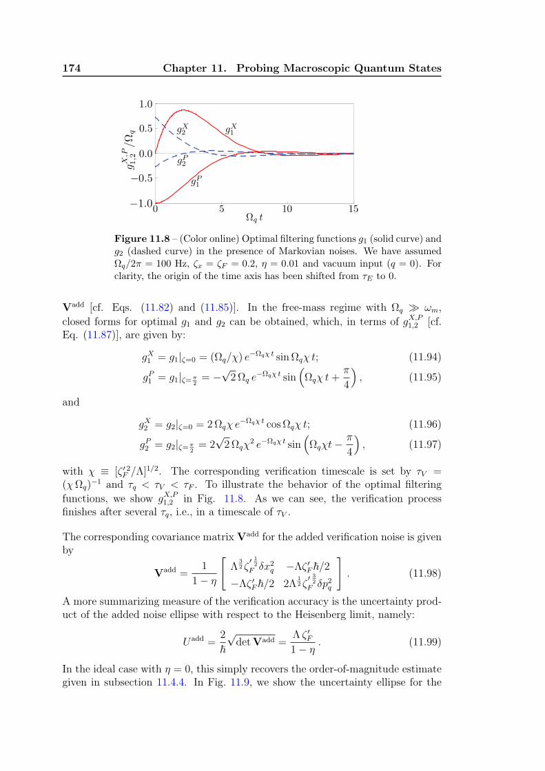
174 Chapter 11. Probing Macroscopic Quantum States
Figure 11.8 – (Color online) Optimal filtering functions g1 (solid curve) andg2 (dashed curve) in the presence of Markovian noises. We have assumedΩq/2π = 100 Hz, ζx = ζF = 0.2, η = 0.01 and vacuum input (q = 0). Forclarity, the origin of the time axis has been shifted from τE to 0.
Vadd [cf. Eqs. (11.82) and (11.85)]. In the free-mass regime with Ωq ≫ ωm,
closed forms for optimal g1 and g2 can be obtained, which, in terms of gX,P1,2 [cf.
Eq. (11.87)], are given by:
gX1 = g1|ζ=0 = (Ωq/χ) e−Ωqχ t sinΩqχ t; (11.94)
gP1 = g1|ζ=π2= −
√2Ωq e
−Ωqχ t sin(Ωqχ t+
π
4
), (11.95)
and
gX2 = g2|ζ=0 = 2Ωqχ e−Ωqχ t cosΩqχ t; (11.96)
gP2 = g2|ζ=π2= 2
√2Ωqχ
2 e−Ωqχ t sin(Ωqχt−
π
4
), (11.97)
with χ ≡ [ζ ′ 2F /Λ]1/2. The corresponding verification timescale is set by τV =
(χΩq)−1 and τq < τV < τF . To illustrate the behavior of the optimal filtering
functions, we show gX,P1,2 in Fig. 11.8. As we can see, the verification process
finishes after several τq, i.e., in a timescale of τV .
The corresponding covariance matrix Vadd for the added verification noise is givenby
Vadd =1
1− η
[Λ
32 ζ
′ 12
F δx2q −Λζ ′F~/2−Λζ ′F~/2 2Λ
12 ζ
′ 32
F δp2q
]. (11.98)
A more summarizing measure of the verification accuracy is the uncertainty prod-uct of the added noise ellipse with respect to the Heisenberg limit, namely:
Uadd =2
~√detVadd =
Λ ζ ′F1− η
. (11.99)
In the ideal case with η = 0, this simply recovers the order-of-magnitude estimategiven in subsection 11.4.4. In Fig. 11.9, we show the uncertainty ellipse for the

11.7. Verification of Macroscopic Quantum Entanglement 175
-1.5-1.0-0.5 0.0 0.5 1.0 1.5-1.5
-1.0
-0.5
0.0
0.5
1.0
1.5
x∆xq
p∆
p q
Figure 11.9 – (Color online) The uncertainty ellipse for the added verifi-cation noise in the presence of Markovian noises. We assume ζx = ζF = 0.2with vacuum input (dashed curve); and ζx = ζF = 0.2 with 10 dB squeezing(dotted curve). For contrast, we also show the Heisenberg limit in a unitcircle, and the ideal conditional quantum state with a solid ellipse.
added noise in the case of ζx = ζF = 0.2, readout loss η = 1% and with (greendotted curve) or without (red long-dashed curve) 10 dB input squeezing. In com-parison, we also plot the Heisenberg limit (unit circle) and the conditional stateobtained through an ideally noiseless state preparation (blue solid ellipse). Asfigure shows, the least challenging scenario already begins to characterize the con-ditional quantum state down to the Heisenberg Uncertainty. In these two cases,we have Λ = 1.48 and 0.62 respectively, leading to:
Uadd = 0.30 (vacuum) , 0.12 (10 dB squeezing). (11.100)
11.7 Verification of Macroscopic Quantum En-
tanglement
In this section, we will apply our protocol to verify macroscopic entanglementbetween test masses in future GW detectors, which was proposed in Refs. [54,129]. In the experiment as shown schematically in Fig. 11.10, measurements at thebright and dark port of the interferometer continuously collapse the quantum stateof the corresponding common and differential modes of the test-mass motion. Thiscreates two highly squeezed Gaussian states in both modes. Since the commonand differential modes are linear combinations of the center of mass motion of testmasses in the two arms, namely xc = xE+ xN and xd = xE− xN, this will naturallygenerate quantum entanglement between the two test masses, which is similar to
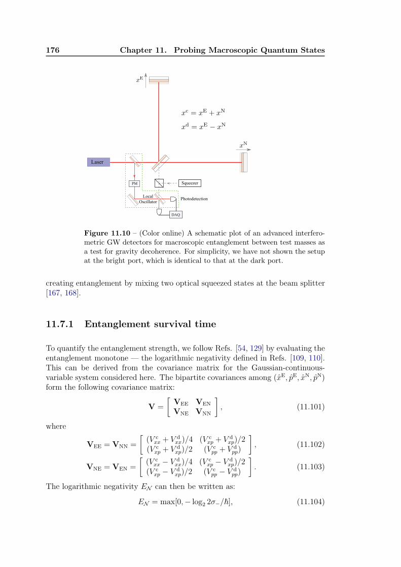
176 Chapter 11. Probing Macroscopic Quantum States
Figure 11.10 – (Color online) A schematic plot of an advanced interfero-metric GW detectors for macroscopic entanglement between test masses asa test for gravity decoherence. For simplicity, we have not shown the setupat the bright port, which is identical to that at the dark port.
creating entanglement by mixing two optical squeezed states at the beam splitter[167, 168].
11.7.1 Entanglement survival time
To quantify the entanglement strength, we follow Refs. [54, 129] by evaluating theentanglement monotone — the logarithmic negativity defined in Refs. [109, 110].This can be derived from the covariance matrix for the Gaussian-continuous-variable system considered here. The bipartite covariances among (xE, pE, xN, pN)form the following covariance matrix:
V =
[VEE VEN
VNE VNN
], (11.101)
where
VEE = VNN =
[(V c
xx + V dxx)/4 (V c
xp + V dxp)/2
(V cxp + V d
xp)/2 (V cpp + V d
pp)
], (11.102)
VNE = VEN =
[(V c
xx − V dxx)/4 (V c
xp − V dxp)/2
(V cxp − V d
xp)/2 (V cpp − V d
pp)
]. (11.103)
The logarithmic negativity EN can then be written as:
EN = max[0,− log2 2σ−/~], (11.104)
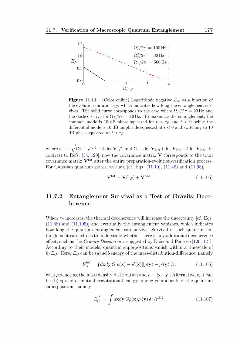
11.7. Verification of Macroscopic Quantum Entanglement 177
Figure 11.11 – (Color online) Logarithmic negative EN as a function ofthe evolution duration τE , which indicates how long the entanglement sur-vives. The solid curve corresponds to the case where ΩF /2π = 20Hz andthe dashed curve for ΩF /2π = 10Hz. To maximize the entanglement, thecommon mode is 10 dB phase squeezed for t > τE and t < 0, while thedifferential mode is 10 dB amplitude squeezed at t < 0 and switching to 10dB phase-squeezed at t > τE .
where σ− ≡√(Σ−
√Σ2 − 4 detV)/2 and Σ ≡ detVNN+detVEE−2 detVNE. In
contrast to Refs. [54, 129], now the covariance matrix V corresponds to the totalcovariance matrix Vtot after the entire preparation-evolution-verification process.For Gaussian quantum states, we have [cf. Eqs. (11.10), (11.48) and (11.98)]
Vtot = V(τE) +Vadd. (11.105)
11.7.2 Entanglement Survival as a Test of Gravity Deco-herence
When τE increases, the thermal decoherence will increase the uncertainty [cf. Eqs.(11.48) and (11.105)] and eventually the entanglement vanishes, which indicateshow long the quantum entanglement can survive. Survival of such quantum en-tanglement can help us to understand whether there is any additional decoherenceeffect, such as the Gravity Decoherence suggested by Diosi and Penrose [120, 121].According to their models, quantum superpositions vanish within a timescale of~/EG. Here, EG can be (a) self-energy of the mass-distribution-difference, namely
E(a)G =
∫dxdyG[ρ(x)− ρ′(x)][ρ(y)− ρ′(y)]/r, (11.106)
with ρ denoting the mass density distribution and r ≡ |x−y|; Alternatively, it canbe (b) spread of mutual gravitational energy among components of the quantumsuperposition, namely
E(b)G =
∫dxdyGρ(x)ρ′(y) δr/r3/2. (11.107)
178 Chapter 11. Probing Macroscopic Quantum States
with δr denoting the uncertainty in location. For the prepared test-mass quantumstates with width of δxq, we have
τ(a)G ≈ Ωq/(Gρ) , τ
(b)G ≈ ~1/2L2Ω1/2
q /(Gm3/2) . (11.108)
where L is the distance between two test masses. Substituting the typical valuesfor LIGO mirrors with ρ = 2.2 g/cm3, the separation between the two input testmasses, L ≈ 10m, and m = 10 kg, we have:
τaG = 4.3× 10⁹ s, τ bG = 1.2× 10⁻⁵ s. (11.109)
It is therefore quite implausible to test model (a); while for model (b), Ωqτ(b)G is
less 0.01 with Ωq/2π = 100 Hz. In Fig. 11.11, we show the entanglement survivalas a function of evolution duration. As we can see, the model (b) of gravitydecoherence can easily be tested, as the entanglement can survive for severaltimes the measurement timescale τq, which is much longer than the predicted τ
(b)G .
11.8 Conclusions
We have investigated in great details a follow-up verification stage after the statepreparation and evolution. We have showed the necessity of a sub-Heisenbergverification accuracy in probing the prepared conditional quantum state, and howto achieve it with an optimal time-domain homodyne detection. Including thisessential building block — a sub-Heisenberg verification, we are able to outline acomplete procedure of a three-staged experiment for testing macroscopic quantummechanics. In particular, we have been focusing on the relevant free-mass regimeand have applied the techniques to discuss MQM experiments with future GWdetectors. However, the system dynamics that have been considered describegeneral cases with a high-Q mechanical oscillator coupled to coherent optical fields.In this respect, we note that our results for Markovian systems only depend onthe ratio between various noises and the SQL, and therefore carries over directlyto systems on other scales. In addition, the Markovian assumption applies moreaccurately to smaller-scale systems which operate at higher frequencies.
11.9 Appendix
11.9.1 Necessity of a sub-Heisenberg accuracy for reveal-ing non-classicality
As we have mentioned in the introduction, a sub-Heisenberg accuracy is a neces-sary condition to probe the non-classicality, if the Wigner function of the prepared

11.9. Appendix 179
quantum state has some negative regions, which do not have any classical coun-terpart.
To prove this necessity, we use the relation between the Q function and the Wignerfunction as pointed out by Khalili [166]. Given density matrix ρ, the Q functionin the coherent state basis |α) is equal to [39, 169, 170]:
Q =1
π(α|ρ|α), (11.110)
which is always positive defined. This is the Fourier transform of the followingcharacteristic function:
J(β, β∗) = Tr[eiβ∗aeiβa
†ρ]. (11.111)
Here, a is the annihilation operator and is related to the normalized oscillatorposition x/δxq and momentum p/δpq [cf. Eq. (11.26)] by the standard relation:
a = [(x/δxq) + i(p/δpq)]/2. (11.112)
If we introduce the real and imaginary parts of β, namely, β = βr + iβi, thecharacteristic function J can be rewritten as:
J(βr, βi) = e−(β2r+β2
i )/2Tr[eiβr(x/δxq)+iβi(p/δpq) ρ], (11.113)
where we have used the fact that eAeB = eA+Be[A, B]/2, as [A, B] commutes withA and B. Inside the bracket of Eq. (11.113), it is the characteristic function forthe Wigner function W (x, p), and thus:
J(βr, βi) =1
(2π)2
∫dx′dp′e−(β2
r+β2i )/2
e−iβr(x′/δxq)−iβi(p′/δpq)W (x′, p′). (11.114)
Integrating over βr and βi, the resulting Q function is given by:
Q(x, p) =1
2π
∫dx′dp′e
− 12
[(x−x′)2
δx2q+
(p−p′)2
δp2q
]W (x′, p′). (11.115)
This will be the same as Eq. (11.7), if we identify Wrecon(x, p) with Q(x, p) and
Vadd =
[δx2q 00 δp2q
], (11.116)
which is a Heisenberg-limited error. Since squeezing and a rotation of x and p axeswill not change the positivity of the Q function, Eq. (11.115) basically dictatesthat the reconstructed Wigner function will always be positive if a Heisenberg-limited error is introduced during the verification stage. Therefore, only if asub-Heisenberg accuracy is achieved will we be able to reveal the non-classicalityof the prepared quantum state.

180 Chapter 11. Probing Macroscopic Quantum States
11.9.2 Wiener-Hopf method for solving integral equations
In this appendix, we will introduce the mathematical method invented by N.Wienerand E. Hopf for solving a special type of integral equations. For more details, onecan refer to a comprehensive presentation of this method and its applications byB. Noble [171]. Here, we will focus on integral equations that can be brought intothe following form, as encountered in obtaining the optimal verification scheme:∫ +∞
0
dt′C(t, t′)g(t′) = h(t) , t > 0 . (11.117)
with
C(t, t′) = A(t− t′) +∑α
∫ min[t,t′]
0
dt′′B∗α(t− t′′)Bα(t
′ − t′′) , (11.118)
where α = 1, 2, . . . and Bα(t) = 0 if t < 0.
Assuming that solution for g(t) to be a square-integrable function in L2(−∞,∞),one can split it into causal and anticausal parts as:
g(t) = g+(t) + g−(t) , (11.119)
where g−(t) is causal part:
g−(t) =
0, t > 0
g(t), t 6 0(11.120)
and g+(t) is the anticausal part of g(t):
g+(t) =
g(t), t > 0
0, t 6 0 .(11.121)
This definition enables us to expand the limits of integration in (11.117) and(11.118) to the full range −∞ < (t, t′, t′′) <∞:∫ +∞
−∞dt′C(t, t′)g+(t
′) = h(t) , t > 0 , (11.122)
where
C(t, t′) = A(t − t′) +∑α
∫ +∞
−∞dt′′[B∗
α,+(t − t′′)Bα,+(t′ − t′′)](+,t′′) , (11.123)
and the index (+, t′′) stands for taking the causal part of a multidimensionalfunction in the argument t′′.

11.9. Appendix 181
Let us first utilize the method in a simple special case when Bα(t) ≡ 0, ∀α, thisgives a conventional Wiener-Hopf integral equation:∫ +∞
0
dt′A(t− t′)g(t′) = h(t) , t > 0 , (11.124)
which can be rewritten as:[∫ +∞
−∞dt′A(t− t′)g+(t
′)− h(t)
](+,t)
= 0 . (11.125)
Applying a Fourier transform in t, and the convolution theorem, one gets:∫ +∞
−∞
dΩ
2π
[A(Ω)g+(Ω)− h(Ω)
]+e−iΩt = 0 . (11.126)
The spectrum of the causal (anticausal) function is simply:
g+(−)(Ω) =
∫ ∞
−∞dt g+(−)(t)e
iΩt . (11.127)
However, this evident relation is not operational for us, as it provides no intuitionon how to directly get g±(Ω) given g(Ω) at our disposal. The surprisingly simpleanswer gives complex analysis. Without loss of generality, we can assume thatg(t) asymptotically goes to zero at infinity as: ∀t : |g(t)| < e−γ0|t| where γ0 is somearbitrary positive number, that guarantees regularity of g(Ω) at −∞ < Ω < ∞.In terms of the analytic continuation g(s) of g(Ω) to the complex plane s = Ω+iγ,the above assumption means that all the poles of g(s) are located outside its bandof analyticity −γ0 < Im(s) < γ0. Thus, the partition into causal and anticausalparts for g(s) is now evident:
g(s) = g+(s) + g−(s) (11.128)
where g+(s)(g−(s)) stands for the function equal to g(s) for γ > γ0(< −γ0) andis analytic in the half plane above (below) the line γ = γ0(−γ0) 3. According toproperties of analytic continuation, this decomposition is unique and completelydetermined by values of g(Ω) on the real axis. Moreover, as a Fourier transform ofvalid L2-function, it has to approach zero when |s| → ∞. For more general cases,this requirement could be relaxed to demand that ∞ should be a regular pointof g(s) so that lim
|s|→∞g(s) = const. This allows to include δ-function and other
integrable distributions into consideration, though it forces us to add the constantg(∞) to formula (11.128) as additional term. For example, for g(t) = e−α|t|, α > 0one has the following Fourier transform:
g(s) =2α
α2 + s2=
2α
(s+ iα)(s− iα)(11.129)
3Functions g+(s) and g−(s) are, in essence, Laplace transforms of g(t) for positive and neg-ative time, respectively, with only a substitution of the variable s → ip.

182 Chapter 11. Probing Macroscopic Quantum States
that has one pole s+ = −iα in the lower half complex plane (LHP) and ones− = +iα in the upper half complex plane (UHP). To split f(Ω) in accordancewith (11.128) one can use the well-known formula:
g±(s) =∑s±,k
Res[g(s), s±,k]
(s− s±,k)σk(11.130)
where summation goes over all poles s+,k (with σk is the order of pole s+,k) ofg(s) that belong to the LHP for g+(s) and over all poles s−,k of g(s) that belongto the UHP for g−(s) otherwise, and Res[g(s), s] stands for residue of g(s) at poles. For our example function this formula gives:
g+(s) =i
s+ iα, g−(s) = − i
s− iα. (11.131)
Using the residue theorem, one can easily show that:
g+(t) = e−αt, for t > 0 (11.132)
g−(t) = eαt, for t < 0 . (11.133)
Coming back to the Eq. (11.126), assume that function A(Ω) can be factorizedin the following way:
A(Ω) = a−(Ω)a+(Ω) (11.134)
where a+(−)(Ω) is a function analytic in the UHP (LHP) with its inverse, ı.e.,both its poles and zeroes are located in the LHP (UHP). One gets the followingequation: [
a−(Ω)a+(Ω)g+(Ω)− h(Ω)]+= 0 . (11.135)
To solve this equation, one realizes the following fact: for any function f , [f(Ω)]+ =0 means that f has no poles in the LHP. Multiplication of f by any function g−which also has no poles in the LHP will evidently not change the equality, namely,[g−(Ω)f(Ω)]+ = 0. Multiplying Eq. (11.135) by 1/a−(Ω), the solution reads
g+(Ω) =1
a+(Ω)
[ h(Ω)a−(Ω)
]+. (11.136)
On performing an inverse Fourier transform of g+(Ω), the time-domain solutiong+(t) can be obtained.
Now we are ready to solve Eq. (11.122) with the general kernel in Eq. (11.123).Performing similar manipulations, one obtains the following equation for g+(Ω)in the Fourier domain:[(
A+∑α
BαB∗α
)g+ −
∑α
Bα(B∗αg+)− − h
]+
= 0 , (11.137)

11.9. Appendix 183
where we have omitted arguments Ω of all functions for brevity. Since Bα is acausal function, B∗
α is anticausal and g+ is causal, (B∗αg)− only depends on the
value of g on the poles of B∗α. Performing a similar factorization:
ψ+ψ− = A+∑α
BαB∗α, (11.138)
with ψ+ (ψ−) and 1/ψ+ (1/ψ−) analytic in the UHP (LHP), ψ+(−Ω) = ψ∗+(Ω) =
ψ−(Ω), we get the solution in the form:
g+ =1
ψ+
[h
ψ−
]+
+1
ψ+
[∑α
Bα(B∗αg+)−
ψ−
]+
. (11.139)
Even though g+ also enters the right hand side of the above equation, yet (B∗αg+)−
can still be written out explicitly as:
(B∗αg+)− =
∑Ω−,k
g+(Ω−,k)Res[B∗(Ω), Ω−,k]
(Ω− Ω−,k)σk. (11.140)
Here Ω−,k are poles of B∗(Ω) that belong to UHP, and therefore g+(Ω−,k) arejust constants that can be obtained by solving a set of linear algebra equations,by evaluating Eq. (11.139) at those poles Ω−,k.
11.9.3 Solving integral equations in Section 11.6
Here, we will use the technique introduced in the previous section to obtain an-alytical solutions to the integral equations we encountered in subsections 11.6.2and 11.6.3.
In the coordinate representation, the integral equations for g1,2 are the following[cf. Eqs. (11.78) and (11.79)]:∫ Tint
0
dt′[C11(t, t
′) C12(t, t′)
C21(t, t′) C22(t, t
′)
] [g1(t
′)g2(t
′)
]=
[0h(t)
], (11.141)
where Cij (i, j = 1, 2) are given by Eqs. (11.88), (11.89) and (11.90), and we havedefined h(t) ≡ µ1f1(t) + µ2f2(t). Since the optimal g1,2(t) will automatically cutoff when t > τF , we can extend the integration upper bound Tint to ∞. Thisbrings the equations into the appropriate form considered in Appendix 11.9.2. Inthe frequency domain, they can be written as
[S11g1]+ + [S12 g2]+ = 0, (11.142)
[S21 g1]+ + [S22 g2]+ − Γ = h, (11.143)
Γ = (1− η)(Ω4q/2)(e
2q + 2ζ2F )[Gx(Gxg2)−]+. (11.144)

184 Chapter 11. Probing Macroscopic Quantum States
Here, Sij are the Fourier transformations of the correlation functions Cij. Specif-ically, they are
S11 =η + (1− η)e2q
2, (11.145)
S12 = −(1− η)e2qΩ2
q
2(Ω + ωm − iγm)(Ω− ωm − iγm), (11.146)
S21 = S∗12, (11.147)
S22 =Λ2
4+
(1− η)(e2q + 2ζ2F )Ω4q
2[(Ω + ωm)2 + γ2m][(Ω− ωm)2 + γ2m]. (11.148)
Since S11 is only a number, the solution to g1 is simply
g1 = −S−111 [S12g2]+. (11.149)
In the time-domain, this recovers the result in Eq. (11.91). Through a spectralfactorization
ψ+ψ− ≡ S22 − S−111 S12S21, (11.150)
we obtain the solution for g2:
g2 =1
ψ+
1
ψ−
[h− S−1
11 S21(S12g2)− + Γ]
+
. (11.151)
Substituting Γ into the above equation, g2 becomes:
g2 =1
ψ+
1
ψ−
[h+ κ Gx(G
∗xg2)−
]+
(11.152)
with κ ≡ m2Ω4qζ
′2F . A simple inverse Fourier transformation gives g1(t) and g2(t).
The unknown Lagrange multipliers can be solved using Eq. (11.83). We canthen derive the covariance matrix Vadd for the added verification noise with Eq.(11.85). In the free-mass regime, a closed form for Vadd can be obtained, as shownexplicitly in Eq. (11.98).

Chapter 12
Conclusions and Future Work
12.1 Conclusions
To conclude, this thesis has covered two main topics concerning MacroscopicQuantum Mechanics (MQM) in optomechanical devices. The first topic con-siders different approaches to surpassing the Standard Quantum Limit (SQL) formeasuring weak forces, which include modifying the input/output optics, and thedynamics of the mechanical oscillator. Concerning the approach of modifyingthe input optics, in Chapter 3, we have proposed simultaneously injecting twosqueezed light—filtered by a resonant optical cavity—into the dark port of thelaser interferometer GW detector. This can reduce the low-frequency radiation-pressure noise, and the high-frequency shot noise so that the detector sensitivityover the entire observational band from 10 Hz to 104 Hz can be improved. Givenits relatively simple setup—only a 30 m filter cavity is required— this could be afeasible add-on to future advanced GW detectors. With the approach of modify-ing the output optics, in Chapter 5, we have proposed the use of a time-domainvariational method, in which the homodyne detection angle has the optimal time-dependence. Such a scheme provides a transparent way to probe the mechanicalquadrature—the conserved dynamical quantity of a mechanical oscillator—andallows us to surpass the SQL. This works in the cases where the bandwidth ofthe optical cavity is much larger than the mechanical frequency, and thereforeit can be implemented in small-scale optomechanical devices, in which high fi-nesse is difficult to achieve, and also in large-scale broadband GW detectors (e.g.,Advanced LIGO). With the approach of modifying the mechanical dynamics, inChapter 4, we have explored the frequency dependence in double optical springs,and we have shown that it can significantly enhance the mechanical response overa broad frequency band. This is especially useful for GW detectors because thenatural frequency of the suspended test-masses is quite low, which gives a lowmechanical response in the detection band around 100 Hz.
The second topic is concerned with exploring quantum behaviors of macroscopicmechanical oscillators with quantum-limited optomechanical devices. In Chapter6, we have discussed the use of three-mode optomechanical interactions to studyMQM. We have pointed out the optimal frequency matching inherent in this in-teraction, which allows a significant enhancement of the optomechanical coupling

186 Chapter 12. Conclusions and Future Work
compared with that in conventional two-mode interactions. Such a feature enablesus to cool milligram-scale mechanical oscillators down to their quantum groundstate and also to create quantum entanglement between the oscillator and thecavity modes. In Chapter 7, we have discussed the quantum limit for groundstate cooling, and the creation of quantum entanglement in general optomechan-ical devices. We have used an alternative point of view, based upon informationloss, to explain the origin of the resolved-sideband cooling limit. By recoveringthe information contained in the cavity output, we can surpass such a coolinglimit without imposing stringent requirements on the cavity bandwidth. We havealso shown such an information recovery can enhance the optomechanical entan-glement. This work can help us in finding the proper parameter regime to achievethe quantum ground state, and to realize quantum entanglement experimentally.In Chapter 8, we have investigated the quantum entanglement between a mechan-ical oscillator and a continuum optical field. In contrast to the cases studied inprevious chapters, the continuum optical field contains infinite degrees of free-dom. We have developed a new functional method to analyze the entanglementstrength, and have derived an elegant scaling which shows that the entanglementonly depends on ratio of the optomechanical coupling to the thermal decoherencestrength. This illuminates the possibility of incorporating mechanical degrees offreedom for future quantum computing at high environmental temperature. InChapter 9, we have studied nonlinear optomechanical interactions for observingmechanical energy quantization. We have derived a simple quantum limit thatonly involves the fundamental parameters of an optomechanical device—this re-quires the zero-point uncertainty of the mechanical oscillator to be comparableto the linear dynamical range of the cavity, which is quantified by the ratio ofthe optical wavelength to the cavity finesse. This limit applies universally toall optomechanical devices, and therefore it serves as a guiding tool for choosingthe right parameters for MQM experiments. In Chapter 10, we have discussedpreparing a mechanical oscillator in non-Gaussian quantum states to explore thenon-classical features of optomechanical devices. We have proposed transferring anon-Gaussian quantum state from the optical field to the mechanical oscillator byinjecting a single-photon pulse into the dark port of an interferometric optome-chanical device. The radiation pressure of the single-photon pulse is coherentlyamplified by the strong optical power from the bright port, which makes such astate transfer possible. We have shown the experimental feasibility in the case ofboth small-scale table-top experiments, and large-scale advanced GW detectors.In Chapter 11, we have outlined a complete procedure for an MQM experiment, byincluding a verification stage to follow up the preparation stage. With an optimaltime-dependent homodyne detection, the prepared quantum state can be probedand verified with a sub-Heisenberg accuracy. This not only allows us to explorethe quantum dynamics of the mechanical oscillator, but also the non-classical fea-ture of the quantum state. In particular, we have applied it to study the survivalduration of the quantum entanglement between macroscopic test-masses whichsuffer from thermal decoherence. This complete procedure can also be directly

12.2. Future work 187
applied to small-scale optomechanical devices.
12.2 Future work
There are still many issues that need to be further investigated for a thoroughunderstanding. Particularly, in Chapter 4, only preliminary results are obtained:they only show the modified mechanical response due to the double optical springbut not the resulting detector sensitivity. We need to combine the outputs ofthe two optical fields in an optimal way to maximize the detector sensitivity. Inaddition, the resulting system is dynamically unstable and we need to figure outa way to control such an instability. In Chapter 5, we have assumed no opticalloss in the variational readout, which certainly fails actually. If the optical lossis included, total evasion of the measurement back-action is not obviously theoptimum as we have found when studying the verification problem in Chapter 11.Since the mathematical structure of this problem is quite different from that in theverification case, we need to find a new method to realize such an optimization. InChapter 9, we have studied the optomechanical dynamics by using the Langevinequation approach. This shows how the dynamical quantities evolve, but the effectof measurement on the evolution of the quantum state is not discussed. Therefore,it is necessary for us to use a different approach to study how the mechanicaloscillator jumps among different energy eigenstates, while at the same time being,subjected to both a continuous measurement and thermal decoherence. This canhelp us to address the question of whether the quantum-Zeno effect exists or notin such a nonlinear optomechanical system. In Chapter 11, we have assumedthat the thermal force noise and measurement sensing noise are white with flatnoise spectra—a Markovian assumption. Non-Markovian noises certainly arise inan actual GW detector. These noises at low frequencies, such as the suspensionthermal noise and the coating thermal noise, tend to rise faster than what wehave assumed. We have already developed the right tools to treat such non-Markovianity but need further analysis to go through the details.


Chapter 13
List of Publications
1 Haixing Miao, Chunong Zhao, Li Ju, Slawek Gras, Pablo Barriga, ZhongyangZhang, and David G. Blair, Three-mode optoacoustic parametric interactionswith a coupled cavity, Phys. Rev. A 78, 063809 (2008).
2 Haixing Miao, Chunnong Zhao, Li Ju and David G. Blair, Quantum ground-state cooling and tripartite entanglement with three-mode optoacoustic inter-actions, Phys. Rev. A 79, 063801 (2009).
3 Chunnong Zhao, Li Ju, Haixing Miao, Slawomir Gras, Yaohui Fan, andDavid G. Blair, Three-Mode Optoacoustic Parametric Amplifier: A Tool forMacroscopic Quantum Experiments, Phys. Rev. Lett. 102, 243902 (2009).
4 Farid Ya. Khalili, Haixing Miao, and Yanbei Chen, Increasing the sensitivityof future gravitational-wave detectors with double squeezed-input, Phys. Rev.D 80, 042006 (2009).
5 Haixing Miao, Stefan Danilishin, Thomas Corbitt, and Yanbei Chen, Stan-dard Quantum Limit for Probing Mechanical Energy Quantization, Phys.Rev. Lett. 103, 100402 (2009).
6 Haixing Miao, Stefan Danilishin, Helge Muller-Ebhardt, Henning Rehbein,Kentaro Somiya, and Yanbei Chen, Probing macroscopic quantum stateswith a sub-Heisenberg accuracy, Phys. Rev. A 81, 012114 (2010).
7 Haixing Miao, Stefan Danilishin, and Yanbei Chen, Universal quantum en-tanglement between an oscillator and continuous fields, Phys. Rev. A 81,052307 (2010).
8 Haixing Miao, Stefan Danilishin, Helge Muller-Ebhardt, and Yanbei Chen,Achieving ground state and enhancing optomechanical entanglement by re-covering information, New Journal of Physics, 12, 083032 (2010).
9 Farid Ya. Khalili, Stefan Danilishin, Haixing Miao, Helge Muller-Ebhardt,Huan Yang, and Yanbei Chen, Preparing a Mechanical Oscillator in Non-Gaussian Quantum States, Phys. Rev. Lett. 105, 070403 (2010).


Bibliography
[1] F. J. Giessibl, “Advances in atomic force microscopy,” Rev. Mod. Phys., 75,pp. 949–, July 2003. 1, 69
[2] U. Mohideen and A. Roy, “Precision Measurement of the Casimir Forcefrom 0.1 to 0.9 mum,” Phys. Rev. Lett., 81, pp. 4549–, Nov. 1998. 1
[3] http://www.ligo.caltech.edu. 1, 2, 49, 127, 150
[4] http://www.virgo.infn.it. 49
[5] http://geo600.aei.mpg.de. 1, 49
[6] H. J. Kimble, Y. Levin, A. B. Matsko, K. S. Thorne, and S. P. Vyatchanin,“Conversion of conventional gravitational-wave interferometers into quan-tum nondemolition interferometers by modifying their input and/or outputoptics,” Phys. Rev. D, 65, 022002, 2001. 3, 37, 51, 52, 54, 62, 105, 158,171, 173
[7] T. Corbitt, N. Mavalvala, and S. Whitcomb, “Optical cavities as amplitudefilters for squeezed fields,” Phys. Rev. D, 70, pp. 022002–, July 2004. 3, 49,50, 51
[8] A. Buonanno and Y. Chen, “Quantum noise in second generation, signal-recycled laser interferometric gravitational-wave detectors,” Phys. Rev. D,64, 042006, 2001. 4, 32, 42, 50, 52, 93
[9] T. Corbitt, Y. Chen, E. Innerhofer, H. Muller-Ebhardt, D. Ottaway, H. Re-hbein, D. Sigg, S. Whitcomb, C. Wipf, and N. Mavalvala, “An All-OpticalTrap for a Gram-Scale Mirror,” Phys. Rev. Lett., 98, pp. 150802–4, Apr.2007. 4, 7, 42, 78, 100, 118, 150
[10] H. Rehbein, H. Muller-Ebhardt, K. Somiya, S. L. Danilishin, R. Schn-abel, K. Danzmann, and Y. Chen, “Double optical spring enhancementfor gravitational-wave detectors,” Phys. Rev. D, 78, 062003, 2008. 4, 42,63, 67
[11] F. Y. Khalili and Y. Levin, “Speed meter as a quantum nondemolitionmeasuring device for force,” Phys. Rev. D, 54, 004735, 1996. 5, 44, 50
[12] P. Purdue, “Analysis of a quantum nondemolition speed-meter interferom-eter,” Phys. Rev. D, 66, 022001, 2002. 44
[13] P. Purdue and Y. Chen, “Practical speed meter designs for quantum non-demolition gravitational-wave interferometers,” Phys. Rev. D, 66, 122004,2002. 38, 39, 45, 51

192 Bibliography
[14] Y. Chen, “Sagnac interferometer as a speed-meter-type, quantum-nondemolition gravitational-wave detector,” Phys. Rev. D, 67, 122004,2003. 44, 47
[15] S. L. Danilishin, “Sensitivity limitations in optical speed meter topology ofgravitational-wave antennas,” Phys. Rev. D, 69, pp. 102003–, May 2004.5, 50
[16] V. B. Braginsky, Y. I. Vorontsov, and K. S. Thorne, “Quantum Nondemo-lition Measurements,” Science, 209, pp. 547–557, Aug. 1980. 6, 70
[17] S. P. Vyatchanin and A. B. Matsko, “Quantum limit on force measure-ments,” JETP, 77, 218, 1993. 6, 39, 51, 69
[18] S. P. Vyatchanin and E. A. Zubova, “Quantum variation measurement of aforce,” Physics Letters A, 201, pp. 269–274, May 1995. 6, 39, 69, 155, 171
[19] P. F. Cohadon, A. Heidmann, and M. Pinard, “Cooling of a Mirror byRadiation Pressure,” Phys. Rev. Lett., 83, pp. 3174–, Oct. 1999. 7, 78, 100,118, 150
[20] C. H. Metzger and K. Karrai, “Cavity cooling of a microlever,” Nature,432, pp. 1002–1005, Dec. 2004. 150
[21] A. Naik, O. Buu, M. D. LaHaye, A. D. Armour, A. A. Clerk, M. P. Blencowe,and K. C. Schwab, “Cooling a nanomechanical resonator with quantumback-action,” Nature, 443, pp. 193–196, Sept. 2006. 78, 129, 150
[22] S. Gigan, H. R. Bohm, M. Paternostro, F. Blaser, G. Langer, J. B.Hertzberg, K. C. Schwab, D. Bauerle, M. Aspelmeyer, and A. Zeilinger,“Self-cooling of a micromirror by radiation pressure,” Nature, 444, pp. 67–70, Nov. 2006. 150
[23] O. Arcizet, P.-F. Cohadon, T. Briant, M. Pinard, and A. Heidmann,“Radiation-pressure cooling and optomechanical instability of a micromir-ror,” Nature, 444, pp. 71–74, Nov. 2006.
[24] D. Kleckner and D. Bouwmeester, “Sub-kelvin optical cooling of a microme-chanical resonator,” Nature, 444, pp. 75–78, Nov. 2006.
[25] A. Schliesser, P. Del’Haye, N. Nooshi, K. J. Vahala, and T. J. Kippenberg,“Radiation Pressure Cooling of a Micromechanical Oscillator Using Dynam-ical Backaction,” Phys. Rev. Lett., 97, pp. 243905–4, Dec. 2006.
[26] T. Corbitt, C. Wipf, T. Bodiya, D. Ottaway, D. Sigg, N. Smith, S. Whit-comb, and N. Mavalvala, “Optical Dilution and Feedback Cooling of aGram-Scale Oscillator to 6.9 mK,” Phys. Rev. Lett., 99, pp. 160801–4,Oct. 2007.

Bibliography 193
[27] A. Schliesser, R. Riviere, G. Anetsberger, O. Arcizet, and T. J. Kippenberg,“Resolved-sideband cooling of a micromechanical oscillator,” Nat Phys, 4,pp. 415–419, May 2008. 150
[28] M. Poggio, C. L. Degen, H. J. Mamin, and D. Rugar, “Feedback Coolingof a Cantilever’s Fundamental Mode below 5 mK,” Phys. Rev. Lett., 99,pp. 017201–4, July 2007. 78, 150
[29] I. Favero, C. Metzger, S. Camerer, D. Konig, H. Lorenz, J. P. Kotthaus,and K. Karrai, “Optical cooling of a micromirror of wavelength size,” Appl.Phys. Lett., 90, pp. 104101–3, Mar. 2007. 150
[30] J. D. Teufel, J. W. Harlow, C. A. Regal, and K. W. Lehnert, “DynamicalBackaction of Microwave Fields on a Nanomechanical Oscillator,” Phys.Rev. Lett., 101, pp. 197203–4, Nov. 2008.
[31] J. D. Thompson, B. M. Zwickl, A. M. Jayich, F. Marquardt, S. M. Girvin,and J. G. E. Harris, “Strong dispersive coupling of a high-finesse cavity toa micromechanical membrane,” Nature, 452, pp. 72–75, Mar. 2008. 9, 78,129, 130, 131, 134, 135, 138, 141
[32] C. M. Mow-Lowry, A. J. Mullavey, S. Gossler, M. B. Gray, and D. E. Mc-Clelland, “Cooling of a Gram-Scale Cantilever Flexure to 70 mK with aServo-Modified Optical Spring,” Phys. Rev. Lett., 100, pp. 010801–4, Jan.2008. 78, 150
[33] S. Groblacher, S. Gigan, H. R. Bohm, A. Zeilinger, and M. Aspelmeyer,“Radiation-pressure self-cooling of a micromirror in a cryogenic environ-ment,” EPL (Europhysics Letters), 81, no. 5, pp. 54003–, 2008. 150
[34] S. W. Schediwy, C. Zhao, L. Ju, D. G. Blair, and P. Willems, “Observationof enhanced optical spring damping in a macroscopic mechanical resonatorand application for parametric instability control in advanced gravitational-wave detectors,” Phys. Rev. A, 77, pp. 013813–5, Jan. 2008. 78, 150
[35] G. Jourdan, F. Comin, and J. Chevrier, “Mechanical Mode Dependence ofBolometric Backaction in an Atomic Force Microscopy Microlever,” Phys.Rev. Lett., 101, pp. 133904–4, Sept. 2008. 150
[36] S. Groblacher, J. B. Hertzberg, M. R. Vanner, G. D. Cole, S. Gigan,K. C. Schwab, and M. Aspelmeyer, “Demonstration of an ultracold micro-optomechanical oscillator in a cryogenic cavity,” Nat Phys, 5, pp. 485–488,July 2009. 150
[37] L. S. Collaboration, “Observation of a kilogram-scale oscillator near itsquantum ground state,” New Journal of Physics, 11, no. 7, pp. 073032–,2009. 7, 100, 118, 150

194 Bibliography
[38] A. Hopkins, K. Jacobs, S. Habib, and K. Schwab, “Feedback cooling of ananomechanical resonator,” Phys. Rev. B, 68, pp. 235328–, Dec. 2003. 7,100, 108, 139, 150
[39] C. Gardiner and P. Zoller, Quantum Noise. Springer-Verlag, 2004. 103, 120,132, 146, 179
[40] G. J. Milburn, “Classical and quantum conditional statistical dynamics,”Quantum and Semiclassical Optics: Journal of the European Optical SocietyPart B, 8, no. 1, pp. 269–, 1996.
[41] A. C. Doherty, S. M. Tan, A. S. Parkins, and D. F. Walls, “State deter-mination in continuous measurement,” Phys. Rev. A, 60, pp. 2380–, Sept.1999. 150
[42] A. C. Doherty and K. Jacobs, “Feedback control of quantum systems usingcontinuous state estimation,” Phys. Rev. A, 60, pp. 2700–, Oct. 1999. 7,100, 108, 139
[43] S. Danilishin, H. Mueller-Ebhardt, H. Rehbein, K. Somiya, R. Schnabel,K. Danzmann, T. Corbitt, C. Wipf, N. Mavalvala, and Y. Chen, “Creationof a quantum oscillator by classical control,” arXiv:0809.2024, 2008. 7, 100,101, 110, 111, 118, 150
[44] F. Marquardt, J. P. Chen, A. A. Clerk, and S. M. Girvin, “Quantum Theoryof Cavity-Assisted Sideband Cooling of Mechanical Motion,” Phys. Rev.Lett., 99, pp. 093902–, Aug. 2007. 8, 78, 83, 85, 86, 96, 100, 101, 103, 130,143, 145
[45] I. Wilson-Rae, N. Nooshi, W. Zwerger, and T. J. Kippenberg, “Theory ofGround State Cooling of a Mechanical Oscillator Using Dynamical Backac-tion,” Phys. Rev. Lett., 99, pp. 093901–, Aug. 2007. 8, 78, 83, 85, 86, 100,101, 103, 118, 143, 145, 150
[46] C. K. Law and H. J. Kimble, “Deterministic generation of a bit-stream ofsingle-photon pulses,” Journal of Modern Optics, 44, no. 11, pp. 2067–2074,1997. 8, 138
[47] J. McKeever, A. Boca, A. D. Boozer, R. Miller, J. R. Buck, A. Kuzmich,and H. J. Kimble, “Deterministic Generation of Single Photons from OneAtom Trapped in a Cavity,” Science, 303, pp. 1992–1994, Mar. 2004.
[48] M. Keller, B. Lange, K. Hayasaka, W. Lange, and H. Walther, “Continuousgeneration of single photons with controlled waveform in an ion-trap cavitysystem,” Nature, 431, pp. 1075–1078, Oct. 2004. 8, 138
[49] A. Einstein, B. Podolsky, and N. Rosen, “Can Quantum-Mechanical De-scription of Physical Reality Be Considered Complete?,” Phys. Rev., 47,pp. 777–, May 1935. 9

Bibliography 195
[50] D. Bouwmeester, A. Ekert, and A. Zeilinger, The Physics of Quantum In-formation. Springer-Verlag, 2002. 9, 99, 118
[51] D. Vitali, S. Gigan, A. Ferreira, H. R. Bohm, P. Tombesi, A. Guerreiro,V. Vedral, A. Zeilinger, and M. Aspelmeyer, “Optomechanical Entangle-ment between a Movable Mirror and a Cavity Field,” Phys. Rev. Lett., 98,pp. 030405–, Jan. 2007. 9, 78, 87, 90, 91, 101, 112, 118, 119, 123, 130
[52] S. Mancini, V. Giovannetti, D. Vitali, and P. Tombesi, “Entangling Macro-scopic Oscillators Exploiting Radiation Pressure,” Phys. Rev. Lett., 88,pp. 120401–, Mar. 2002. 9, 118
[53] M. J. Hartmann and M. B. Plenio, “Steady State Entanglement in the Me-chanical Vibrations of Two Dielectric Membranes,” Phys. Rev. Lett., 101,pp. 200503–, Nov. 2008. 78, 101, 118, 119, 123
[54] H. Mueller-Ebhardt, H. Rehbein, R. Schnabel, K. Danzmann, and Y. Chen,“Entanglement of Macroscopic Test Masses and the Standard QuantumLimit in Laser Interferometry,” Phys. Rev. Lett., 100, pp. 013601–, Jan.2008. 9, 10, 78, 99, 101, 118, 119, 130, 150, 154, 175, 176, 177
[55] V. B. Braginsky, “Classical and Quantum Restrictions on the Detection ofWeak Disturbances of a Macroscopic Oscillator,” JETP, 26, 831, 1968. 14,15, 50, 61, 151
[56] C. M. Caves, K. S. Thorne, R. W. Drever, V. D. Sandberg, and M. Zimmer-mann, “On the measurement of a weak classical force coupled to a quantum-mechanical oscillator. I. Issues of principle,” Rev. Mod. Phys., 52, 341,1980.
[57] V. B. Braginsky and F. Y. Khalili, Quantum Measurement. CambridgeUniversity Press, 1992. 15, 34, 35, 61
[58] C. M. Caves and B. L. Schumaker, “New formalism for two-photon quan-tum optics. I - Quadrature phases and squeezed states. II - Mathematicalfoundation and compact notation,” Phys. Rev. A, 31, 3068, 1985. 16, 158
[59] K. J. Blow, R. Loudon, S. J. D. Phoenix, and T. J. Shepherd, “Continuumfields in quantum optics,” Phys. Rev. A, 42, 4102, 1990. 18, 158
[60] R. W. P. Drever, Gravitational Radiation. North-Holland, 1983. 29
[61] J. Y.Vinet, B. Meers, C. Man, and A. Brillet, “Optimization of long-baselineoptical interferometers for gravitational-wave detection,” Phys. Rev. D, 38,433, 1988. 31
[62] B. J. Meers, “Recycling in laser-interferometric gravitational-wave detec-tors,” Phys. Rev. D, 38, 2317, 1988. 31, 93

196 Bibliography
[63] A. Buonanno and Y. Chen, “Signal recycled laser-interferometergravitational-wave detectors as optical springs,” Phys. Rev. D, 65, 042001,2002. 32, 41, 50, 65, 68
[64] A. Buonanno and Y. Chen, “Scaling law in signal recycled laser-interferometer gravitational-wave detectors,” Phys. Rev. D, 67, 062002,2003. 32, 36, 50, 52, 54, 63, 65, 66, 104
[65] J. Mizuno, Comparison of Optical Configurations for Laser-InterferometricGravitational-Wave Detectors. PhD thesis, Max-Planck Institut fur Quan-tenoptik, Garching, Germany,, 1995. 32, 65
[66] J. Mizuno, K. A. Strain, P. G. Nelson, J. M. Chen, R. Schilling, A. Rudiger,W. Winkler, and K. Danzmann, “Resonant sideband extraction: a newconfiguration for interferometric gravitational wave detectors,” Phys. Lett.A, 175, 273, 1993. 32
[67] J. Harms, Y. Chen, S. Chelkowski, A. Franzen, H. Vahlbruch, K. Danz-mann, and R. Schnabel, “Squeezed-input, optical-spring, signal-recycledgravitational-wave detectors,” Phys. Rev. D, 68, 042001, 2003. 38
[68] V. B. Braginsky, M. L. Gorodetsky, and F. Y. Khalili, “Optical bars ingravitational wave antennas,” Phys. Lett. A, 232, 340, 1997. 41
[69] V. B. Braginsky, M. L. Gorodetsky, F. Y. Khalili, and K. S. Thorne, “Noisein gravitational-wave detectors and other classical-force measurements is notinfluenced by test-mass quantization,” Phys. Rev. D, 61, 044002, 2000. 44,50
[70] F. Y. Khalili, “Increasing future gravitational-wave detectors’ sensitivity bymeans of amplitude filter cavities and quantum entanglement,” Phys. Rev.D, 77, pp. 062003–, Mar. 2008. 49, 50, 51, 52, 53, 55
[71] http://tamago.mtk.nao.ac.jp. 49
[72] http://www.ligo.caltech.edu/advLIGO. 49, 69, 138
[73] K. S. Thorne, Three Hundred Years of Gravitation. Cambridg UniversityPress, 1987. 50
[74] V. B. Braginsky and F. Y. Khalili, Quantum Measurement. CambridgeUniversity Press, 1992. 50, 69, 70, 99, 118, 123, 137, 147, 151, 163
[75] V. B. Braginsky and F. Y. Khalili, “Low noise rigidity in quantum measure-ments,” Physics Letters A, 257, pp. 241–246, July 1999. 50
[76] F. Y. Khalili, “Frequency-dependent rigidity in large-scale interferometricgravitational-wave detectors,” Physics Letters A, 288, pp. 251–256, Oct.2001. 50

Bibliography 197
[77] E. G. Unruh, Quantum Optics, Experimental Gravitation, and MeasurementTheory. Springer-Verlag, 1982. 51
[78] F. Khalili, “Limiting sensitivity during the continuous tracking of the coor-dinates of a quantum test system,” Akademiia Nauk SSSR, Doklady, 294,603, 1987. 51
[79] M. T. Jaekel and S. Reynaud, “Quantum Limits in Interferometric Mea-surements,” EPL (Europhysics Letters), 13, no. 4, pp. 301–, 1990.
[80] A. F. Pace, M. J. Collett, and D. F. Walls, “Quantum limits in interfero-metric detection of gravitational radiation,” Phys. Rev. A, 47, pp. 3173–,Apr. 1993.
[81] A. Buonanno and Y. Chen, “Improving the sensitivity to gravitational-wavesources by modifying the input-output optics of advanced interferometers,”Phys. Rev. D, 69, pp. 102004–, May 2004.
[82] O. Arcizet, T. Briant, A. Heidmann, and M. Pinard, “Beating quantumlimits in an optomechanical sensor by cavity detuning,” Phys. Rev. A, 73,pp. 033819–, Mar. 2006.
[83] F. Y. Khalili, V. I. Lazebny, and S. P. Vyatchanin, “Sub-standard-quantum-limit sensitivity via optical rigidity in the advanced LIGO interferometerwith optical losses,” Phys. Rev. D, 73, pp. 062002–, Mar. 2006. 51
[84] K. McKenzie, N. Grosse, W. P. Bowen, S. E. Whitcomb, M. B. Gray, D. E.McClelland, and P. K. Lam, “Squeezing in the Audio Gravitational-WaveDetection Band,” Phys. Rev. Lett., 93, pp. 161105–, Oct. 2004. 51
[85] H. Vahlbruch, S. Chelkowski, B. Hage, A. Franzen, K. Danzmann, andR. Schnabel, “Coherent Control of Vacuum Squeezing in the Gravitational-Wave Detection Band,” Phys. Rev. Lett., 97, pp. 011101–, July 2006. 51
[86] K. A. Postnov and L. R. Yungelson, “The Evolution of Compact BinaryStar Systems,” Living Reviews in Relativity, 9, pp. –, Dec. 2006. 56
[87] I. S. Kondrashov, D. A. Simakov, F. Y. Khalili, and S. L. Danilishin, “Op-timizing the regimes of the Advanced LIGO gravitational wave detector formultiple source types,” Phys. Rev. D, 78, pp. 062004–, Sept. 2008. 56
[88] http://ilog.ligo wa.caltech.edu:7285/advligo/Bench. 56
[89] L. S. Collaboration, “First upper limits from LIGO on gravitational wavebursts,” Phys. Rev. D, 69, pp. 102001–, May 2004. 56
[90] Y. Chen, S. L. Danilishin, F. Y. Khalili, and H. Mller-Ebhardt, “QND mea-surements for future gravitational-wave detectors,” arXiv:0910.0319, 2009.62
198 Bibliography
[91] H. Mueller-Ebhardt, On quantum effects in the dynamics of macroscopictest masses. PhD thesis, Leibniz University Hannover, 2009. 63
[92] A. A. Clerk, F. Marquardt, and K. Jacobs, “Back-action evasion and squeez-ing of a mechanical resonator using a cavity detector,” New Journal ofPhysics, 10, no. 9, pp. 095010–, 2008. 71
[93] S. L. Danilishin, F. Y. Khalili, and S. P. Vyatchanin, “The discrete samplingvariation measurement,” Physics Letters A, 278, pp. 123–128, Dec. 2000.72, 74
[94] S. L. Danilishin and F. Y. Khalili, “Stroboscopic variation measurement,”Physics Letters A, 300, pp. 547–558, Aug. 2002. 72
[95] V. B. Braginsky, S. E. Strigin, and S. P. Vyatchanin, “Parametric oscillatoryinstability in Fabry-Perot interferometer,” Physics Letters A, 287, pp. 331–338, Sept. 2001. 77, 78, 80, 81, 84
[96] C. Genes, D. Vitali, P. Tombesi, S. Gigan, and M. Aspelmeyer, “Ground-state cooling of a micromechanical oscillator: Comparing cold damping andcavity-assisted cooling schemes,” Phys. Rev. A, 77, pp. 033804–, Mar. 2008.78, 143, 145
[97] S. Mancini, D. Vitali, and P. Tombesi, “Scheme for Teleportation of Quan-tum States onto a Mechanical Resonator,” Phys. Rev. Lett., 90, pp. 137901–, Apr. 2003. 78, 130, 139
[98] M. Paternostro, D. Vitali, S. Gigan, M. S. Kim, C. Brukner, J. Eisert, andM. Aspelmeyer, “Creating and Probing Multipartite Macroscopic Entangle-ment with Light,” Phys. Rev. Lett., 99, pp. 250401–, Dec. 2007. 78, 87, 88,89, 91, 99, 101
[99] V. B. Braginsky, S. E. Strigin, and S. P. Vyatchanin, “Analysis of paramet-ric oscillatory instability in power recycled LIGO interferometer,” PhysicsLetters A, 305, pp. 111–124, Dec. 2002. 78
[100] C. Zhao, L. Ju, J. Degallaix, S. Gras, and D. G. Blair, “Parametric Insta-bilities and Their Control in Advanced Interferometer Gravitational-WaveDetectors,” Phys. Rev. Lett., 94, pp. 121102–, Apr. 2005.
[101] L. Ju, S. Gras, C. Zhao, J. Degallaix, and D. Blair, “Multiple modes contri-butions to parametric instabilities in advanced laser interferometer gravita-tional wave detectors,” Physics Letters A, 354, pp. 360–365, June 2006.
[102] A. Gurkovsky, S. Strigin, and S. Vyatchanin, “Analysis of parametric oscil-latory instability in signal recycled LIGO interferometer,” Physics LettersA, 362, pp. 91–99, Feb. 2007. 78

Bibliography 199
[103] V. B. Braginsky and S. P. Vyatchanin, “Low quantum noise tranquilizerfor Fabry-Perot interferometer,” Physics Letters A, 293, pp. 228–234, Feb.2002. 78
[104] S. Gras, D. Blair, and L. Ju, “Test mass ring dampers with minimum ther-mal noise,” Physics Letters A, 372, pp. 1348–1356, Feb. 2008. 78
[105] C. Zhao, L. Ju, Y. Fan, S. Gras, B. J. J. Slagmolen, H. Miao, P. Bar-riga, D. G. Blair, D. J. Hosken, A. F. Brooks, P. J. Veitch, D. Mudge,and J. Munch, “Observation of three-mode parametric interactions in longoptical cavities,” Phys. Rev. A, 78, pp. 023807–, Aug. 2008. 78
[106] C. Zhao, L. Ju, H. Miao, S. Gras, Y. Fan, and D. G. Blair, “Three-ModeOptoacoustic Parametric Amplifier: A Tool for Macroscopic Quantum Ex-periments,” Phys. Rev. Lett., 102, pp. 243902–, June 2009. 79, 86, 100,118, 150
[107] H. Miao, C. Zhao, L. Ju, S. Gras, P. Barriga, Z. Zhang, and D. G. Blair,“Three-mode optoacoustic parametric interactions with a coupled cavity,”Phys. Rev. A, 78, pp. 063809–, Dec. 2008. 79
[108] C. Genes, D. Vitali, and P. Tombesi, “Simultaneous cooling and entan-glement of mechanical modes of a micromirror in an optical cavity,” NewJournal of Physics, 10, no. 9, pp. 095009–, 2008. 86, 89, 100, 103, 107, 118,150
[109] G. Vidal and R. F. Werner, “Computable measure of entanglement,” Phys.Rev. A, 65, pp. 032314–, Feb. 2002. 87, 112, 113, 119, 121, 176
[110] G. Adesso and F. Illuminati, “Entanglement in continuous-variable systems:recent advances and current perspectives,” Journal of Physics A: Mathemat-ical and Theoretical, 40, no. 28, pp. 7821–, 2007. 87, 89, 112, 121, 176
[111] A. Peres, “Separability Criterion for Density Matrices,” Phys. Rev. Lett.,77, pp. 1413–, Aug. 1996. 89, 112
[112] R. Simon, “Peres-Horodecki Separability Criterion for Continuous VariableSystems,” Phys. Rev. Lett., 84, pp. 2726–, Mar. 2000. 112
[113] A. Serafini, “Multimode Uncertainty Relations and Separability of Contin-uous Variable States,” Phys. Rev. Lett., 96, pp. 110402–, Mar. 2006. 89,119
[114] D. Reitze, “LIGO R&D documents: LIGO-G050360-00-R,” 2005. 91
[115] J. Laurat, G. Keller, J. Augusto, J. A. Oliveira-Huguenin, C. Fabre,T. Coudreau, A. Serafini, G. Adesso, and F. Illuminati, “Entanglement

200 Bibliography
of two-mode Gaussian states: characterization and experimental produc-tion and manipulation,” Journal of Optics B: Quantum and SemiclassicalOptics, 7, no. 12, pp. S577–, 2005. 91
[116] M. Rakhmanov, Dynamics of Laser Interferometric Gravitational Wave De-tectors. PhD thesis, California Institute of Technology, 2000. 93
[117] G. Mueller, “LIGO document: G070441-00-R,” 2007. 93
[118] W. H. Zurek, “Decoherence and the Transition from Quantum to Classical,”Phys. Today, 44, pp. 36–44, Oct. 1991. 99
[119] L. Diosi, “A universal master equation for the gravitational violation ofquantum mechanics,” Physics Letters A, 120, pp. 377–381, Mar. 1987.
[120] L. Diosi, “Models for universal reduction of macroscopic quantum fluctua-tions,” Phys. Rev. A, 40, pp. 1165–, Aug. 1989. 154, 160, 177
[121] R. Penrose, “On Gravity’s role in Quantum State Reduction,” General Rel-ativity and Gravitation, 28, pp. 581–600, May 1996. 99, 154, 160, 177
[122] A. D. O’Connell, M. Hofheinz, M. Ansmann, R. C. Bialczak, M. Lenander,E. Lucero, M. Neeley, D. Sank, H. Wang, M. Weides, J. Wenner, J. M.Martinis, and A. N. Cleland, “Quantum ground state and single-phononcontrol of a mechanical resonator,” Nature, 464, pp. 697–703, Apr. 2010.100, 118, 138
[123] D. G. Blair, E. N. Ivanov, M. E. Tobar, P. J. Turner, F. van Kann, andI. S. Heng, “High Sensitivity Gravitational Wave Antenna with ParametricTransducer Readout,” Phys. Rev. Lett., 74, pp. 1908–, Mar. 1995. 100,118, 150
[124] S. Vyatchanin, “Effective cooling of quantum system,” Dokl. Akad. NaukSSSR, 234, 688, 1977. 100, 118, 150
[125] S. Mancini, D. Vitali, and P. Tombesi, “Optomechanical Cooling of a Macro-scopic Oscillator by Homodyne Feedback,” Phys. Rev. Lett., 80, pp. 688–,Jan. 1998. 101
[126] L. Diosi, “Laser linewidth hazard in optomechanical cooling,” Phys. Rev.A, 78, pp. 021801–, Aug. 2008.
[127] P. Rabl, C. Genes, K. Hammerer, and M. Aspelmeyer, “Phase-noise inducedlimitations on cooling and coherent evolution in optomechanical systems,”Phys. Rev. A, 80, pp. 063819–, Dec. 2009. 100, 118, 150
[128] F. Elste, S. M. Girvin, and A. A. Clerk, “Quantum Noise Interferenceand Backaction Cooling in Cavity Nanomechanics,” Phys. Rev. Lett., 102,pp. 207209–, May 2009. 100, 135

Bibliography 201
[129] H. Mueller-Ebhardt, H. Rehbein, C. Li, Y. Mino, K. Somiya, R. Schn-abel, K. Danzmann, and Y. Chen, “Quantum-state preparation and macro-scopic entanglement in gravitational-wave detectors,” Phys. Rev. A, 80,pp. 043802–, Oct. 2009. 100, 108, 143, 146, 148, 150, 151, 154, 155, 158,159, 165, 175, 176, 177
[130] W. Marshall, C. Simon, R. Penrose, and D. Bouwmeester, “Towards Quan-tum Superpositions of a Mirror,” Phys. Rev. Lett., 91, pp. 130401–, Sept.2003. 101
[131] H. Miao, S. Danilishin, and Y. Chen, “Universal Quantum Entanglementbetween an Oscillator and Continuous Fields,” arXiv:0908.1053, 2009. 101,113, 114
[132] M. O. Scully and K. Druhl, “Quantum eraser: A proposed photon corre-lation experiment concerning observation and ”delayed choice” in quantummechanics,” Phys. Rev. A, 25, pp. 2208–, Apr. 1982. 101, 112
[133] Y.-H. Kim, R. Yu, S. P. Kulik, Y. Shih, and M. O. Scully, “Delayed ”Choice”Quantum Eraser,” Phys. Rev. Lett., 84, pp. 1–, Jan. 2000. 101
[134] M. Horodecki, P. Horodecki, and R. Horodecki, “Separability of mixedstates: necessary and sufficient conditions,” Physics Letters A, 223, pp. 1–8, Nov. 1996. 112, 119
[135] A. Ferreira, A. Guerreiro, and V. Vedral, “Macroscopic Thermal Entangle-ment Due to Radiation Pressure,” Phys. Rev. Lett., 96, pp. 060407–, Feb.2006. 119
[136] S. Pirandola, S. Mancini, D. Vitali, and P. Tombesi, “Continuous-variableentanglement and quantum-state teleportation between optical and macro-scopic vibrational modes through radiation pressure,” Phys. Rev. A, 68,pp. 062317–, Dec. 2003. 119, 125
[137] L.-M. Duan, G. Giedke, J. I. Cirac, and P. Zoller, “Inseparability Criterionfor Continuous Variable Systems,” Phys. Rev. Lett., 84, pp. 2722–, Mar.2000. 119
[138] R. F. Werner and M. M. Wolf, “Bound Entangled Gaussian States,” Phys.Rev. Lett., 86, pp. 3658–, Apr. 2001. 121
[139] H. Miao, S. Danilishin, H. Mueller-Ebhardt, H. Rehbein, K. Somiya, andY. Chen, “Probing macroscopic quantum states with a sub-Heisenberg ac-curacy,” Phys. Rev. A, 81, pp. 012114–, Jan. 2010. 122, 123, 126, 144
[140] C. Genes, A. Mari, P. Tombesi, and D. Vitali, “Robust entanglement of amicromechanical resonator with output optical fields,” Phys. Rev. A, 78,pp. 032316–, Sept. 2008. 124, 125

202 Bibliography
[141] D. H. Santamore, A. C. Doherty, and M. C. Cross, “Quantum nondemolitionmeasurement of Fock states of mesoscopic mechanical oscillators,” Phys.Rev. B, 70, pp. 144301–, Oct. 2004. 129, 130
[142] I. Martin and W. H. Zurek, “Measurement of Energy Eigenstates by a SlowDetector,” Phys. Rev. Lett., 98, pp. 120401–, Mar. 2007. 129, 138
[143] K. Jacobs, P. Lougovski, and M. Blencowe, “Continuous Measurement ofthe Energy Eigenstates of a Nanomechanical Resonator without a Nonde-molition Probe,” Phys. Rev. Lett., 98, pp. 147201–, Apr. 2007. 130, 138,154
[144] M. Bhattacharya and P. Meystre, “Trapping and Cooling a Mirror to ItsQuantum Mechanical Ground State,” Phys. Rev. Lett., 99, pp. 073601–,Aug. 2007. 131
[145] A. M. Jayich, J. C. Sankey, B. M. Zwickl, C. Yang, J. D. Thompson, S. M.Girvin, A. A. Clerk, F. Marquardt, and J. G. E. Harris, “Dispersive op-tomechanics: a membrane inside a cavity,” New Journal of Physics, 10,no. 9, pp. 095008–, 2008. 131
[146] D. I. Schuster, A. A. Houck, J. A. Schreier, A. Wallraff, J. M. Gambetta,A. Blais, L. Frunzio, J. Majer, B. Johnson, M. H. Devoret, S. M. Girvin,and R. J. Schoelkopf, “Resolving photon number states in a superconductingcircuit,” Nature, 445, pp. 515–518, Feb. 2007. 131
[147] A. A. Clerk and D. W. Utami, “Using a qubit to measure photon-numberstatistics of a driven thermal oscillator,” Phys. Rev. A, 75, pp. 042302–,Apr. 2007. 131, 138
[148] A. A. Clerk, M. H. Devoret, S. M. Girvin, F. Marquardt, and R. J.Schoelkopf, “Introduction to Quantum Noise, Measurement and Amplifi-cation,” arXiv:0810.4729, 2008. 132
[149] F. Marquardt and S. M. Girvin, “Optomechanics (a brief review),” Physics,2, 40, 2009. 137
[150] A. J. Leggett, “Macroscopic Quantum Systems and the Quantum Theory ofMeasurement,” Progress of Theoretical Physics Supplement, 69, 80, 1980.137
[151] J. S. Bell, Speakable and Unspeakable in Quantum Mechanics. CambridgeUniversity Press, 1987. 137
[152] S. L. Braunstein and P. van Loock, “Quantum information with continuousvariables,” Rev. Mod. Phys., 77, pp. 513–, June 2005. 137

Bibliography 203
[153] H. Miao, S. Danilishin, T. Corbitt, and Y. Chen, “Standard QuantumLimit for Probing Mechanical Energy Quantization,” Phys. Rev. Lett., 103,pp. 100402–, Sept. 2009. 138
[154] D. Kleckner, I. Pikovski, E. Jeffrey, L. Ament, E. Eliel, J. van den Brink,and D. Bouwmeester, “Creating and verifying a quantum superpositionin a micro-optomechanical system,” New Journal of Physics, 10, no. 9,pp. 095020–, 2008. 138
[155] J. Zhang, K. Peng, and S. L. Braunstein, “Quantum-state transfer fromlight to macroscopic oscillators,” Phys. Rev. A, 68, pp. 013808–, July 2003.138
[156] O. Romero-Isart, M. L. Juan, R. Quidant, and J. I. Cirac, “Toward QuantumSuperposition of Living Organisms,” arXiv:0909.1469, 2009. 139
[157] B. Julsgaard, J. Sherson, J. I. Cirac, J. Fiurasek, and E. S. Polzik, “Ex-perimental demonstration of quantum memory for light,” Nature, 432,pp. 482–486, Nov. 2004. 140, 143, 148
[158] P. Marek and R. Filip, “Noise resilient quantum interface based on QNDinteraction,” arXiv:1002.0225. 140, 143, 148
[159] A. Barchielli, “Stochastic differential equations anda posteriori states inquantum mechanics,” International Journal of Theoretical Physics, 32,pp. 2221–2233, Dec. 1993. 150
[160] S. Miyoki, T. Uchiyama, K. Yamamoto, H. Hayakawa, K. Kasahara, H. Ishit-suka, M. Ohashi, K. Kuroda, D. Tatsumi, S. Telada, M. Ando, T. Tomaru,T. Suzuki, N. Sato, T. Haruyama, Y. Higashi, Y. Saito, A. Yamamoto,T. Shintomi, A. Araya, S. Takemoto, T. Higashi, H. Momose, J. Akamatsu,and W. Morii, “Status of the CLIO project,” Classical and Quantum Grav-ity, 21, no. 5, pp. S1173–, 2004. 150
[161] A. I. Lvovsky and M. G. Raymer, “Continuous-variable optical quantum-state tomography,” Rev. Mod. Phys., 81, pp. 299–, Mar. 2009. 153
[162] B. Yurke and D. Stoler, “Measurement of amplitude probability distribu-tions for photon-number-operator eigenstates,” Phys. Rev. A, 36, pp. 1955–,Aug. 1987. 153
[163] S. Mancini, V. I. Man’ko, and P. Tombesi, “Ponderomotive control of quan-tum macroscopic coherence,” Phys. Rev. A, 55, pp. 3042–, Apr. 1997. 154
[164] S. Bose, K. Jacobs, and P. L. Knight, “Preparation of nonclassical states incavities with a moving mirror,” Phys. Rev. A, 56, pp. 4175–, Nov. 1997.

204 Bibliography
[165] I. Katz, A. Retzker, R. Straub, and R. Lifshitz, “Signatures for a Classicalto Quantum Transition of a Driven Nonlinear Nanomechanical Resonator,”Phys. Rev. Lett., 99, pp. 040404–, July 2007.
[166] F. Khalili, S. Danilishin, H. Miao, H. Muller-Ebhardt, H. Yang, andY. Chen, “Preparing a mechanical oscillator in non-Gaussian quantumstates,” submitted to PRL, 2010. 154, 179
[167] A. Furusawa, J. L. S03rensen, S. L. Braunstein, C. A. Fuchs, H. J. Kimble,and E. S. Polzik, “Unconditional Quantum Teleportation,” Science, 282,pp. 706–709, Oct. 1998. 176
[168] W. P. Bowen, R. Schnabel, P. K. Lam, and T. C. Ralph, “ExperimentalInvestigation of Criteria for Continuous Variable Entanglement,” Phys. Rev.Lett., 90, pp. 043601–, Jan. 2003. 176
[169] M. O. Scully and M. S. Zubairy, Quantum Optics. Cambridg UniversityPress, 1997. 179
[170] D. F. Walls and G. Milburn, Quantum Optics. Springer-Verlag, 2008. 179
[171] B. Nobel, Methods Based on the Wiener-Hopf Technique for the Solution ofPartial Differential Equations. AMS Chelsea Publishing, 1988. 180