exploring the foundation of quantum information in quantum
TRANSCRIPT

Exploring the Foundation ofQuantum Information in Quantum
Optics
by
Xian Ma
A thesispresented to the University of Waterloo
in fulfillment of thethesis requirement for the degree of
Doctor of Philosophyin
Physics
Waterloo, Ontario, Canada, 2016
c© Xian Ma 2016

I hereby declare that I am the sole author of this thesis. This is a true copy of the thesis,including any required final revisions, as accepted by my examiners.
I understand that my thesis may be made electronically available to the public.
ii

Abstract
Quantum information is promising in solving certain computational problems and in-formation security. The power of its speed up and privacy is based on one of the mosttested physical theory: quantum mechanics. Many of the promises of quantum informationhas already been demonstrated in different implementations, which could also be viewedas witness of quantum mechanics. As we progress further in quantum information, we findthat some of the aspects of quantum mechanics could be tested in a novel way. Performingthose tests may lead to new physical theory or at least reinforce our belief of the accuracyof quantum mechanics. In this thesis, I report a few different approaches in testing thefoundation of quantum mechanics using results obtained from quantum optics. While de-veloping such test, quantum state tomography is heavily used to characterize our system.I also report a simplified way of performing quantum state tomography for quantum statethat is close to pure state.
iii

Acknowledgements
I am deeply indebted to my parents Jianlin Zhang and Jianhua Ma for everything. Iwant to thank my wife Xue Rui and my daughter Reyna Ma for their love and support.I must thank Dr. Raymond Laflamme, for giving me the opportunity to be part of hisresearch group, for his constant support and guidance. I must thank the members of myadvisory committee; Dr. Jonathan Baugh, Dr. Joseph Emerson, and Dr. Frank Wilhelmfor their interest in my research and for their support. I am thankful to everyone at theIQC.
iv

Table of Contents
List of Tables vii
List of Figures viii
1 Introduction 1
2 Background: quantum optics and quantum information 3
2.1 Quantum optics . . . . . . . . . . . . . . . . . . . . . . . . . . . . . . . . . 3
2.1.1 Photon modes and evolution . . . . . . . . . . . . . . . . . . . . . . 3
2.1.2 Parametric down converted photons . . . . . . . . . . . . . . . . . . 4
2.1.3 Dual-rail qubits and its relation to polarization qubits . . . . . . . . 8
2.1.4 Unitary gates for photon-polarization qubits . . . . . . . . . . . . . 9
2.2 Quantum information . . . . . . . . . . . . . . . . . . . . . . . . . . . . . . 10
2.2.1 Quantum state tomography and Maximum Likelihood Estimation . 10
3 Testing quantum foundations in space using artificial satellite 13
3.1 Introduction . . . . . . . . . . . . . . . . . . . . . . . . . . . . . . . . . . . 13
3.2 T. Ralph and G. Milburn’s alternative quantum optics theory . . . . . . . 14
3.3 Testing quantum mechanics with artificial satellites . . . . . . . . . . . . . 16
v

4 Testing envariance 20
4.1 Introduction . . . . . . . . . . . . . . . . . . . . . . . . . . . . . . . . . . . 20
4.2 Deriving Born rule from envariance . . . . . . . . . . . . . . . . . . . . . . 21
4.3 Experimental testing envariance . . . . . . . . . . . . . . . . . . . . . . . . 25
4.4 Bounds to Born rule . . . . . . . . . . . . . . . . . . . . . . . . . . . . . . 32
4.5 Conclusion . . . . . . . . . . . . . . . . . . . . . . . . . . . . . . . . . . . . 35
5 Pure State Tomography using Pauli Observables 38
5.1 Introduction . . . . . . . . . . . . . . . . . . . . . . . . . . . . . . . . . . . 38
5.2 Historical results on UDP and UDA . . . . . . . . . . . . . . . . . . . . . . 40
5.3 2 qubit pure state tomography using Paulis measurements . . . . . . . . . 41
5.4 3 qubit pure state tomography using Paulis measurements . . . . . . . . . 43
5.5 Pure state tomography in NMR system . . . . . . . . . . . . . . . . . . . . 45
5.5.1 Pure state tomography for a 2-qubit state . . . . . . . . . . . . . . 46
5.5.2 Pure state tomography for 3-qubit state . . . . . . . . . . . . . . . 47
5.6 Pure state tomography for polarized photon qubits . . . . . . . . . . . . . 49
6 Conclusion 55
References 57
APPENDICES 63
A Testing of envariance to Born rule continued 64
B Proof of UDA using selected Paulis for 3 qubits 70
vi

List of Tables
4.1 Wave plate setting used to implement polarization rotations. . . . . . . . . 27
4.2 Summary of the results for comparing stages I and III . . . . . . . . . . . 31
vii

List of Figures
2.1 Generation of polarization entangled photons via parametric down conversion 7
3.1 Proposed scheme testing gravitationally induced decorrelation . . . . . . . 17
3.2 Coincidence rate prediction for testing gravitationally induced decorrelation 18
4.1 Experimental setup for testing envariance . . . . . . . . . . . . . . . . . . . 26
4.2 Experimental measurement procedure of testing envariance . . . . . . . . . 28
4.3 Reconstructed density matrix of the initial state from the source, after im-plement the first rotation and final state . . . . . . . . . . . . . . . . . . . 29
4.4 Analysis of the experimental results for testing envariance. . . . . . . . . . 30
4.5 Generalized correlations for the singlet state as a function of n using Son’stheory [1]. . . . . . . . . . . . . . . . . . . . . . . . . . . . . . . . . . . . . 34
4.6 Correlation functions versus the rotation angle φ. . . . . . . . . . . . . . . 36
5.1 NMR experiment substance . . . . . . . . . . . . . . . . . . . . . . . . . . 46
5.2 Pure state tomography for 2 qubits . . . . . . . . . . . . . . . . . . . . . . 48
5.3 Performance of 2-qubit protocol using selected Pauli measurements againstrandomly Pauli measurements. . . . . . . . . . . . . . . . . . . . . . . . . . 49
5.4 scheme to create the GHZ state via global controls in NMR . . . . . . . . . 50
5.5 Pure state tomography for GHZ state. . . . . . . . . . . . . . . . . . . . . 51
5.6 Performance of 3-qubit protocol using selected Pauli measurements againstrandomly Pauli measurements. . . . . . . . . . . . . . . . . . . . . . . . . . 52
5.7 Measurement scheme for a polarization-encoded n-photon state. . . . . . . 53
viii

A.1 Testing “Fine graining”. . . . . . . . . . . . . . . . . . . . . . . . . . . . . 67
A.2 Preparation of entangled state α|00〉+ β|11〉 . . . . . . . . . . . . . . . . . 68
ix

Chapter 1
Introduction
Quantum Mechanics is arguably the most tested physical theory in human history. It hasbeen directly and indirectly tested in numerous experiments since its discovery in the early20th century. Many promises of quantum mechanics has been realized such as transistorand atomic clock, and those discovery are verification of quantum mechanics themselves.Moreover, with the help of those technology, one was able to design more precise exper-iments testing quantum mechanics. In the past few decades, quantum information wasdeveloped to help us understand unique advantages of quantum mechanics over classicalcounter parts such as computational power and information security. It has been realized inmany systems such as NMR, optics, superconducting electrode and ion trap. It is anotherpiece of evidence that quantum mechanics as we known is accurate. A natural questionarises: could one use quantum information as a tool to further test quantum mechanics?
The key to above question is knowing what to test. As many existing proposal oftesting quantum mechanics pointed out, to test a theory, one should find some generalizedtheory that reduce to the original one when certain parameters become negligible. Thedevelopment of quantum information gave us many different angles to look at quantummechanics, which gave birth to a few theories which one could use to test the foundationof quantum mechanics.
Many predecessors have proposed and performed tests to quantum mechanics. LikeSteven Weinberg in the 80s who proposed a family of generalization to quantum mechanicswhich could be tested using spinning particles in external fields. In that work, he pointsout the inconsistency of many other attempts to generalize the quantum mechanics byintroducing non-linear terms in the Schrodinger equation. From a mathematician’s per-spective, Andrew M. Gleason proved that for a system whose state lives in a separable
1

Hilbert space of complex dimension at least 3, an unique trace class operator exist for anyquantum probability measurement with Hermitian observables. In other words, Born ruleof probability naturally follows when we describe our state in the complex Hilbert space,and require probability measurement to be non-negative and always normalized under dif-ferent basis. More recently, a 3-slit photon interference experiment is done which putbounds on deviations from the Born rule. The success of quantum mechanics in varioustest and the incompatibility with general relativity motivate us to seek different angle inthe test of quantum foundations.
In this thesis, I am going focus on two separate proposal testing quantum mechanics.First is to look at gravitationally induced entanglement de-correlation[2]. A generalizedtheory proposed by Ralph and Milburn in a sequences of papers gives entangled photonstraveling in curved space time some additional de-correlation due to an additional degreeof freedom from the said theory. This theory is adopted to develop potential experimentproposal for a satellite with only quantum uplink capacity. Second, we turn our attentionto environmental induced invariance(envariance), and its application to test quantum me-chanics. The symmetry of envariance could be used to explain decoherence and thereforebypass the need of introducing Born rule as an axiom of quantum mechanics. In an opticsexperiment, we tested this symmetry and used the result to bound the Born rule using cer-tain extended theory of quantum mechanics[3]. At last, we discuss something we discoveralong the line while we are investigating the above tests: the tomography of quantum statethat is close to a pure state using Pauli observables. When dealing with state that is closeto pure state, we discovered that much less quantum operation are needed to reconstructour quantum state compared to the general case. For two and three qubits system, welisted the minimum number of Pauli operation required to perform tomography on a purequantum state, and tested the robustness in experiments[4].
My contribution of the thesis have already been published in the following papers:
[1] D Rideout, T Jennewein, G Amelino-Camelia, T F Demarie, B L Higgins, A Kempf,A Kent, R Lalamme, X Ma, R B Mann, et al. Fundamental quantum optics experimentsconceivable with satellitesreaching relativistic distances and velocities. Classical and Quan-tum Gravity, 29(22):224011, 2012.
[2] L Vermeyden, X Ma, J Lavoie, M Bonsma, Urbasi Sinha, R Laflamme, and KJ Resch.Experimental test of environment-assisted invariance. Physical Review A, 91(1):012120,2015.
[3] X Ma, T Jackson, H Zhou, J Chen, D Lu, M D Mazurek, K AG Fisher, X Peng,D Kribs, K J Resch, Z Ji, B Zeng, and R Laflamme Pure-state tomography with theexpectation value of Pauli operators.Physical Review A, 93(3):032140, 2016.
2

Chapter 2
Background: quantum optics andquantum information
In this chapter, we are going to introduce some basic background material in quantumoptics and quantum information, which would be useful to understand the subsequentchapters. It will also serve to establish the notation and terminology used in this work.The background material is separated into two sections: Section 2.1, Quantum optics andSection 2.2, Quantum information. Both will give the basic information that is requiredand direct to more resources if interested.
2.1 Quantum optics
2.1.1 Photon modes and evolution
First, we would like to expand the optical fields over a set of modes a1, a†1, a2, a
†2....
For convenience, we pick aki and akj to be orthogonal modes when ki 6= kj. Therefore,operators aki and akj have boson commutation relations
[aki , akj ] = [a†ki , a†kj
] = 0 (2.1)
[aki , a†kj
] = δkikj (2.2)
In Heisenberg picture, the quantum modes of the output state could be write as rearrange-ment of the modes and their conjugates. Without losing generality, we define the evolution
3

to bebk = fk(a1, a
†1, a2, a
†2...) (2.3)
where bk is the output mode k. In other word, if we have a detector designed to measuremode k at the output, the mode arrived at the detector would be bk. The form of fk dependson the unitary(or sometimes non-unitary) evolution U(a1, a
†1, a2, a
†2...) we are interested in.
Here, we assume this initial state is the vacuum state, where ak|0〉 = 0 for any mode k.We can consider the expectation value for a photon number at detector k of the form
n = 〈0|b†kbk|0〉. (2.4)
Moreover, if we measure the correlation between modes ki and kj, the coincidence is givenby
Ckikj = 〈0|b†ki bki b†kjbkj |0〉. (2.5)
2.1.2 Parametric down converted photons
To create entangled photons, one would require nonlinear interaction between photons.One of the most common nonlinear interaction is the parametric down conversion. Ithappens when photon modes enters a medium with nonlinear susceptibility tensor χ, wherethe dielectric polarization density could be expressed as
P (t) = ε0(χ(1)E(t) + χ(2)E2(t) + χ(3)E3(t) + ...), (2.6)
where ε0 is the vacuum permittivity and E(t) is the electrical field. The coefficients χ(n)
are the n-th order susceptibility, and we are interested in the nonlinear effects due to theχ(2) term. The interaction Hamiltonian of the parametric down conversion has the form ofan integral over the volmue of the crystal [5]
HI(t) =ε0χ
(2)
2
∫V
dV E(+)p E(−)
s E(−)i + h.c., (2.7)
where E(+)p is the positive frequency part of the pump optical field, E
(−)s and E
(−)i are
the negative frequency part of the signal and idler optical field, respectively. Using thisHamiltonian, it is possible to generate pairs of entangled photons. In this section we aregoing to consider a simple case where all pump, signal and idler modes are single modeplane waves traveling in the z direction. For a more general derivation, please see Ref. [5]and [6].
4

Under our plane wave assumption, the field operators could be expressed as
E(+)p = i
√~ωp2ε0V
ap exp[i(kpz − ωpt)], (2.8)
E(−)s = −i
√~ωs
2ε0Va†s exp[−i(ksz − ωst)], (2.9)
E(−)i = −i
√~ωi
2ε0Va†i exp[−i(kiz − ωit)]. (2.10)
where ap is the annihilation operator for the pump, a†s and a†i are creation operators forthe signal and the idler respectively.
If the signal and the idler are initialize as vacuum state and the pump initialized in acoherent state, where the wave function at t = 0 is |φ(0)〉 = |α〉p|0〉s|0〉i. The wave functionof the three modes in the first-order perturbation theory takes the form
|φ(t)〉 = |φ(0)〉+1
i~
∫ t
0
dt′HI(t′)|φ(0)〉
= |φ(0)〉+1
i~
∫ t
0
dt′ε0χ
(2)
2
∫V
dV E(+)p E(−)
s E(−)i |φ(0)〉
= |φ(0)〉 − ε0χ(2)
2~(
~2ε0V
)32√ωsωiωp
∫ t
0
dt′∫V
dV ap exp[i(kpz − ωpt′)]
×a†s exp[−i(ksz − ωst′)]a†i exp[−i(kiz − ωit′)]|φ(0)〉
= |φ(0)〉 − ε0χ(2)
2~(
~2ε0V
)32√ωsωiωp
∫ t
0
dt′∫V
dV exp[i(kp − ks − ki)z]
× exp[i(ωs + ωi − ωp)t′]apa†sa†i |φ(0)〉 (2.11)
If we ignore the pump and output vacuum state, the second term in Eq 2.11 gives us wavefunction of a photon pair
|ψ(t)〉 = −αε0χ(2)
2~(
~2ε0V
)32√ωsωiωp
∫ t
0
dt′∫V
dV exp[i(kp−ks−ki)z] exp[i(ωs+ωi−ωp)t′]|1〉s|1〉i.
(2.12)We could make a few observations by looking at this wave function. First, since theinteraction time t is usually much longer than the optical frequency. We have∫ t
0
dt′ exp[i(ωs + ωi − ωp)t′] ≈∫ ∞
0
dt′ exp[i(ωs + ωi − ωp)t′] = 2πδ(ωs + ωi − ωp), (2.13)
5

so the frequencies of the two photon should satisfy
ωs + ωi = ωp. (2.14)
This is the energy conservation of the process. Moreover, if we assume the interactionhappen in a area with length and L, we have∫ L
0
dz exp[i(kp − ks − ki)z] = exp[i(kp − ks − ki)L
2]sinc[(kp − ks − ki)
L
2]. (2.15)
In order to maximize the entangled photon output, the function sinc[(kp − ks − ki)L2]
needs to be maximized. This is called phase matching. Note that we used the first-orderperturbation theory in Eq 2.11. The higher order terms in the series of expansion wouldlead to terms describing multiple photons generated in each mode. It is worth pointingout that those multiple photon output are not simply product of entangle pairs[7].
Energy-time entangled photons
As described in Eq 2.14, the two photons generated by parametric down conversion havenatural correlation in energy. This could be used to produce energy-time entangled pho-tons [8][9] that we use later in Chapter 3.
To verify the idler and the signal photon are indeed entangled, one could measureboth photons in distant detectors. If the difference of arrival time ti and ts violates∆(ti − ts)∆(ωi + ωs) > 1, it is sufficient to show bipartite entanglement between thetwo photons[10]. With the energy conservation ωs + ωi = ωp, the inequality could besimplified as ∆(ti − ts)∆(ωp) > 1.
Polarization entangled photons
To discuss the polarization entangled photon, it is important to review the polarizationstates of photon pairs generated by parametric down conversion. There are two typescorrelated polarizations. When the signal and idler photons have parallel polarization,it is called type I correlation. When the signal and idler photons have perpendicularpolarizations, it is called type II correlation. In this section, we are going to introduceone method to generate polarization entangled photons using type II parametric downconversion, which we use later in Chapter 4. For other interesting methods to generatepolarization entangled photons please refer to Ref [11].
6

Figure 2.1: Preparation of polarization entangled photons. The blue line represents thepump beam, which gets removed at filter(IF). The pink and purple lines represent the signaland idler. The pump light is a 45 degree polarized beam. The horizontal photons from thepump beam travels counterclockwise after the polarizing beam splitter, and generate pairsof horizontal idler and vertical signal photons through type II PDC at PPKTP. The verticalphotons from the pump beam travels clockwise, and generate pairs of vertical idler andhorizontal signal photons. The half wave plate is put in for phase matching purpose. Astwo path are indistinguishable, we create polarization entangled photons at the couplers.
7

As shown in Fig 2.1, we input a 45 degree polarized pump beam:
|ψ〉 =1√2
(|H〉+ |V 〉). (2.16)
The horizontal photons from the pump beam gets transmitted at the polarizing beamsplitter, and generating horizontal idler and vertical signal photons at the nonlinear crystalPPKTP. The horizontal idler gets transmitted by the polarized beam splitter to the couplerA, while the vertical signal gets reflected to the coupler B. Therefore, the setup producesthe transformation |H〉 → |H〉A|V 〉B. The vertical photons from the pump beam getsreflected at the polarizing beam splitter, and generating vertical idler and horizontal signalphotons. The vertical idler gets reflected by the polarized beam splitter to the coupler A,while the horizontal signal gets transmitted to the coupler B. Therefore, the setup producesthe transformation |V 〉 → |V 〉A|H〉B. Since to path are indistinguishable, we arrived atpolarization entangled state:
|φ〉 =1√2
(|H〉A|V 〉B + |V 〉A|H〉B). (2.17)
By adjusting the angle of the QWP at the couple A, we could produce
|φ〉 =1√2
(|H〉A|V 〉B + eiθ|V 〉A|H〉B). (2.18)
By tilting the quarter wave plate, this source generates two of the four Bell states.
2.1.3 Dual-rail qubits and its relation to polarization qubits
In the original linear optics quantum computing scheme [12], dual-rail qubits are used tobuild an ideal quantum computer. The location of a photon in two possible paths areused to encode a qubit. If we name the two spatial mode a and b, the logic 0 is givenby a photon traveling in spatial mode a, |0〉L = |10〉ab, while logic 1 is given by a photontraveling in spatial mode b, |1〉L = |01〉ab. The single qubit unitaries for dual-rail qubitscould be implemented with beam splitters and phase shifters. To show that using bothphase shifters and beam splitters are sufficient for any single qubit gates, we first observethat phase shifter on mode a would give us arbitrary rotation about the Z axis up to aglobal phase. The unitary for a phase shifter placed on the path of mode is given by
UPS(φ) =
(eiφ 00 1
)(2.19)
8

A beam splitter with transmittance sin θ could be described by
UPS(θ) =
(cos θ − sin θsin θ cos θ
)(2.20)
If one put a phase shifter UPS(φ1) after a beam splitter UPS(θ) after a phase shifter UPS(φ1),one could have universal single qubit gate for dual-rail qubits.
UPS(φ2)UPS(θ)UPS(φ1) =
(ei(φ1+φ2) cos θ −eiφ2 sin θeiφ1 sin θ cos θ
)(2.21)
The two polarization degree of freedom for photons, the horizontally and verticallypolarization |H〉, |V 〉, could also be used as basis for implementing qubits. The polarizationqubits can be converted to the dual-rail qubits by introducing a piece of polarized beamsplitter(PBS), which transmits |H〉 and reflects |V 〉. If we name the transmitted spatialmode, mode a, and the reflected mode, mode b. PBS transforms input state α|H〉+ β|V 〉as a polarization qubit to α|10〉ab + β|01〉ab as a dual rail qubit. It is worth noting, onecould easily reverse the setting to convert a dual-rail qubit into a polarization qubit.
2.1.4 Unitary gates for photon-polarization qubits
In order to perform universal one qubit unitary on a photon-polarization qubits, one usessets of waveplates to alter the polarization state of photons traveling through it. Wave-plates are made of birefringent material, whose index of refraction varies depending on thepolarization and propagation direction light. By controlling the thickness of such crystal,one could build half wave plate(HWP) and quarter wave plate(QWP). By rotating themajor axis of HWP or QWP, the waveplates’ unitary changes. For an HWP with its majoraxis at an angle θ, we have
UHWP (θ) = e−iθY e−iπ2ZeiθY
= −i(
cos 2θ sin 2θsin 2θ − cos 2θ
)= −i (Z cos 2θ +X sin 2θ) (2.22)
where X, Y and Z are Pauli Matrices,
X =
(0 11 0
)(2.23)
9

Y =
(0 −ii 0
)(2.24)
Z =
(1 00 −1
)(2.25)
similarly, for a QWP with its major axis at an angle θ, we have
UQWP (θ) = e−iθY e−iπ4ZeiθY
=1√2
(1− i cos (2θ) −i sin 2θ−i sin 2θ 1 + i cos (2θ)
)=
1√2
(1− iX sin 2θ − iZ cos 2θ) (2.26)
Note that using either a single QWP or a HWP will not give us all universal single qubitunitaries by rotating the crystal. Therefore, we stack a few waveplates together to getuniversal single qubit rotations. One of the simplest way to implement it would be tostack a QWP after an HWP and finally after a QWP.
UQWP (θ1)UHWP (θ2)UQWP (θ3)
= Z (cos 2θ2 − cos 2θ3 cos (2θ2 − 2θ1)− sin 2θ3 sin (2θ2 − 2θ1))
Y (sin (2θ3 − 2θ2) + sin (2θ2 − 2θ1))
X (sin 2θ2 − sin 2θ3 cos (2θ2 − 2θ1) + cos 2θ3 sin (2θ2 − 2θ1))
−iI (cos (2θ3 − 2θ2) + cos (2θ2 − 2θ1)) (2.27)
By rotating the major axis of the three crystal, any single qubit gate could be realized bythis set up.
2.2 Quantum information
2.2.1 Quantum state tomography and Maximum Likelihood Es-timation
One key task in quantum information is quantum state tomography, where the density ma-trix representing our quantum state is determined via a number of measurements. With
10
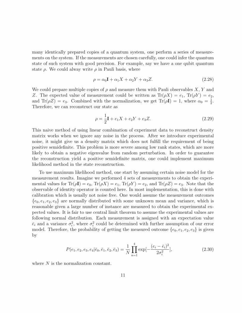
many identically prepared copies of a quantum system, one perform a series of measure-ments on the system. If the measurements are chosen carefully, one could infer the quantumstate of such system with good precision. For example, say we have a one qubit quantumstate ρ. We could alway write ρ in Pauli basis, where
ρ = α0I + α1X + α2Y + α3Z. (2.28)
We could prepare multiple copies of ρ and measure them with Pauli observables X, Y andZ. The expected value of measurement could be written as Tr(ρX) = e1, Tr(ρY ) = e2,and Tr(ρZ) = e3. Combined with the normalization, we get Tr(ρI) = 1, where α0 = 1
2.
Therefore, we can reconstruct our state as
ρ =1
2I + e1X + e2Y + e3Z. (2.29)
This naive method of using linear combination of experiment data to reconstruct densitymatrix works when we ignore any noise in the process. After we introduce experimentalnoise, it might give us a density matrix which does not fulfill the requirement of beingpositive semidefinite. This problem is more severe among low rank states, which are morelikely to obtain a negative eigenvalue from random perturbation. In order to guaranteethe reconstruction yield a positive semidefinite matrix, one could implement maximumlikelihood method in the state reconstruction.
To use maximum likelihood method, one start by assuming certain noise model for themeasurement results. Imagine we performed 4 sets of measurements to obtain the experi-mental values for Tr(ρI) = e0, Tr(ρX) = e1, Tr(ρY ) = e2, and Tr(ρZ) = e3. Note that theobservable of identity operator is counted here. In most implementation, this is done withcalibration which is usually not noise free. One would assume the measurement outcomese0, e1, e2, e3 are normally distributed with some unknown mean and variance, which isreasonable given a large number of instance are measured to obtain the experimental ex-pected values. It is fair to use central limit theorem to assume the experimental values arefollowing normal distribution. Each measurement is assigned with an expectation valueei and a variance σ2
i , where σ2i could be determined with further assumption of our error
model. Therefore, the probability of getting the measured outcome e0, e1, e2, e3 is givenby
P (e1, e2, e3, e4|e0, e1, e2, e3) =1
N
4∏n=1
exp[−(ei − ei)2
2σ2i
], (2.30)
where N is the normalization constant.
11

Instead of directly use the experimentally measured value in our state reconstruction,maximum likelihood estimation tries to find the set of values of the model parameters thatmaximizes the probability of getting the experimentally measured value given such modelparameters. Our optimization task becomes to find such expectation value e0, e1, e2, e3which maximize the probability P (e1, e2, e3, e4|e0, e1, e2, e3). To simplify the expression, wecan take logarithm of Eq. 2.30:
lnP (e1, e2, e3, e4|e0, e1, e2, e3) = − lnN −4∑
n=1
(ei − ei)2
2σ2i
. (2.31)
To further simplify Eq. 2.31, we need to make assumptions on the variances σ2i according
to our physical system. For example, when photon number is measured, we could assumethe measurement outcome follows the Poisson distribution, where σi =
√ei. Therefore,
our optimization task could reduce to finding the minimum of following function:
L(e1, e2, e3, e4|e0, e1, e2, e3) =4∑
n=1
(ei − ei)2
2ei, (2.32)
where L(e1, e2, e3, e4|e0, e1, e2, e3) is called the likelihood function. Some times the varianceσ2i are the same for different measurements, where σi = σ. The optimization is further
reduced to finding the minimum of likelihood function
L(e1, e2, e3, e4|e0, e1, e2, e3) =4∑
n=1
(ei − ei)2, (2.33)
which is also known as the least squares fitting.
12

Chapter 3
Testing quantum foundations inspace using artificial satellite
3.1 Introduction
Quantum mechanics and general relativity are two of the most successful theories in the20th century. Although both of them survived numerous tests with great accuracy, theyare not compatible in certain area. Quantum theory exceptionally describes the behaviourof physical systems at small scales, while general relativity theory predicts systems at largescales. One expects that both theories are limiting cases of one set of unified laws of physics.However, the success of both theory makes it extremely difficult to find experimentalevidence that points us towards such unifying laws of physics.
Going forward, we need more experimental guidance. We could observe and captureevents that naturally occurs in the universe, such as the cosmic microwave background(CMB), which is so far the best potential for solid experimental evidence for quantumgravitational effects. However, the observation of CMB counts only a passive one-shotexperiment since the big bang can not be repeated.
Therefore, it is important that we push our direct tests of quantum theory to scaleswhere the curvature of spacetime is no longer negligible. Some experiments have beenalready performed up to hundreds of kilometers on the Earth[13]. Such tests still fall shortto probe the potential important physics that arises at the intersection of quantum theoryand general relativity. The next step would be looking at potential experiments in evenlarger scale, in the outer space. A test conceivable with artificial satellites in Earth orbit
13

or elsewhere in the solar system may be helpful to eliminate various alternative physicaltheories and place bounds on phenomenological models.
At time of this project was conducted, there was a scientific proposal, where an artificialsatellite with uplink quantum channel capacity would be available. The task was to lookat different alternative physical theories and find ones that have significant difference tothe standard quantum fields theory that could be detected on the satellite.
In this Chapter, we look an alternative quantum optics theory proposed by T. Ralph andG. Milburn in a series of papers. By introducing a second time-like degree of freedom calledevent operator, entangled photon traveling in curved space time would gain additionalde-correlation under this alternative quantum optics theory. My work in this chapteris described in Section 3.3, where we adopted this theory for our uplink satellite anddetermined the required photon detector resolution for the satellite.
3.2 T. Ralph and G. Milburn’s alternative quantum
optics theory
The standard quantum fields theory in curved spacetime [14] allows quantum entanglementto survive unchecked in a wide variety of gravitational environments. Ideally, entangledphotons created locally and traveling through regions of different gravitational backgroundwill still possess all the entanglement they begin with. Local detectors can be carefullydesigned to reveal this. One would need to take into account other factors which mayalso alter the amount entanglement, such as redshift, time-of-arrival delay, phase locking,modification, mode shape, etc. Of course, there is always the possibility that the descrip-tion of standard quantum field is not accurate, and an alternative theory is needed. Analternative theory of the behaviour of photons under different gravitational backgroundwas introduced by Ralph and Milburn in a series of papers [15, 16, 17, 18, 19] originallydesigned to explain the thought experiment of quantum information propagation in pres-ence of closed timelike curves but later used to predict measurable decoherence induced bygravitation.
The motivation of this alternative theory is to allow photon modes to interact with itspast. Under Deutsch model [20] for closed timelike curves, a quantum state is allowed tointeract with a version of itself in the past as long as we enforce the density operator ofthe state to match. This can not be done with photon modes in standard quantum fieldtheory, since the all point along the geodesic of the light ray commutes. This alternativetheory attempts to localize the photon modes in the temporal degree of freedom, so that
14

photon mode of the present and the past no longer commute. This theory also providessome visible changes to entangled pairs traveling in curved spacetime, which could be usedto test the theory.
The essence of this proposal is to supplement ordinary field theory with an additionaldegree of freedom called an event operator, which is associated with the detectors used tomeasure the field quanta in a given setup. In flat spacetime with detectors in the samereference frame, the event operator is of no visible consequence because time passes at thesame rate for all detectors. But when two detectors are in curved spacetime, their localclocks run at different rates and fall out of sync gradually. When the amount by whichthey desynchronize during the photons’ times of flight is longer than the timing resolutionof the detectors, then, although the delay in the time of arrival can be accounted for in thedetector design, the presence of the event operator (whose duration is associated to thedetector’s temporal resolution) ensures that the two photons lose coherence.
What is the event operator? Lets start by writing out the mode annihilation operatorfor a field traveling in the positive x direction:
a(t, x) =
∫dk G(k) eik(x−t+ψ)ak (3.1)
where t is the time, k is the optical frequency and G(k) is a normalized spectral modedistribution and ψ is the phase shift. Note that we have chosen the speed of light to bec = 1 so that the time t is in units of space. It is natural to assume G(k) = 0 for k < 0,since optical modes with negative frequency would not be physical.
It is easy to verify that all points along the geodesic of the light ray are equivalent forthis traveling field. In other word a translation of Eq. 3.1 by x→ x+ δ, t→ t+ δ producesno change in the mode operator:
a(t+ δ, x+ δ) =
∫dk G(k) eik(x+δ−t−δ+ψ)ak = a(t, x). (3.2)
The essence of this alternative quantum optics theory is the event operator. We introduce asecond spectral degree of freedom, Ω, and a distribution, J(Ω), over this degree of freedomto each of the input modes, such that Eq. 3.1 becomes
a(x, t) =
∫dk G(k) eik(x−t+ψ) ×
∫dΩ J(Ω) eiΩtak,Ω (3.3)
where a(x, t) is called the event operator. Note that
[ak,Ω, a†k′,Ω′ ] = δ(k − k′)δ(Ω− Ω′). (3.4)
15

We can view ak,Ω as a description of optical mode localized not only in the frequency kbut also in the second spectral degree of freedom Ω. By adding this independent, localtemporal parametrization of the quantum optical modes, we aim to make observable atdifferent points along the geodesic commute.
3.3 Testing quantum mechanics with artificial satel-
lites
The scheme proposed in Ref. [19] involves preparing a pair of entangled photons via spon-taneous parametric down-conversion (SPDC). One of the entangled photons is measureddirectly on the ground station after a time delay, while the other is sent to the satellite,traversing a varying gravitational potential. Figure 3.1 illustrates the process.
Using the localized event operator introduced in this alternative theory, the maximumcoincidence detection rate of two photons should decline due to intrinsic decoherence bythe curved spacetime. As described earlier in this chapter, the local clock of two detectorexperiencing different gravitational potential falls out of sync. The difference in propertime ∆ between the two detectors during the time of flight of the photons determine thetimescale for the event operators in question, and therefore sets the timescale on whichdecoherence will take place. In our setting, one of the entangled photon is reflected atthe surface of the Earth, and remained in the lab until measured. Therefore it is alwaysat the distance xl = re to the Earth center, where re = 6.38 × 10⁶m is the radius of theEarth. The other photon is sent to the satellite, which is at distance xs = re + h to theEarth center, where h is the height of the satellite. Therefore, in a Schwarzschild metric,the difference in proper time ∆ between the two detectors is given by
∆ = M ln(xsxl
)
≈ Mh
re(3.5)
where 2M = 8.87× 10⁻³m is the Schwarzschild radius of the Earth. When the differencein proper time ∆ is larger than the detector temporal resolution dt, decoherence occurs. Inthe model proposed by Ralph and Milburn in Ref. [19], the reduced correlation function isgiven by
C = Cmax exp
(−∆2
4d2t
), (3.6)
16
the modal functions to occur !as for the classical case" when2#xp−xm+2M ln! xp
xm"$=xd2−xd1 !again with td1= td2 and as-
suming the detectors are far from the massive body". How-ever the size of the maximum is reduced in the event opera-tor formalism. In the limit that !"1 /#J, where #J is thevariance of the distribution J!$" the coincidences will disap-pear to first order in %. Note though that the maximum singledetector count rates remain %%max%2. Thus the effect of thedifferent local propagation times in the event formalism is todecorrelate the entanglement.
To estimate the size of this effect we consider placing thesource and detectors on a geostationary satellite with the mir-ror at ground level and the polarizing beam splitter at heighth. At geostationary orbit the curvature can be neglected, andwe find approximately
! & 2Mh
re. !46"
We assume a Gaussian form for the function J!$",
J!$" =dt
'&e−$2dt
2. !47"
As commented earlier, the effect of the J!$" function is toisolate a localized detection event that is then projected backonto the initial state. It seems natural then to associate dtwith the temporal uncertainty in the measurement. Given thatthe detectors have been positioned to maximize the modalfunctions then the correlation function becomes
C = %%max%2e−!2/4dt2, !48"
and we conclude significant decorrelation will occur when!'2dt. We estimate the intrinsic temporal uncertainty of asilicon photon counter to be around 200 fs and hence set thestandard deviation in units of length to dt=6(10−5 m.Using Eq. !46", the mass of earth in units of length,M =4.4(10−3 m, and the radius of earth re=6.38(106 m,we find this implies significant decorrelation whenh'90 km.
C. Experimental proposal
The estimate at the close of the last section suggests that atestable effect exists for Earth scale curvatures. Nonetheless,directing entangled beams down from geostationary orbit toreflectors separated by a hundred kilometers and back is notcurrently practical. However a slight rearrangement of thesetup, shown in Fig. 4, leads to a more practical proposal. Wenow assume that the source, polarizing beam splitter andsecond detector are all approximately at height xp=re+h,while the mirror, first detector and the correlator are all ap-proximately at ground level, xm=re. A classical channel linksthe second detector and the correlator. Mathematically thesituation is still described by the general equations of theprevious section. In particular it is still possible to maximizethe modal correlation function although clearly we must nowallow for different detection times. The first line of Eq. !45"still describes the magnitude of ! but now with xd1&xm andxd2&xp. With the modal functions maximized !which im-plies xi1=xi2" we have
! & M ln( xp
xm) . !49"
Following the arguments of the previous section we thusconclude that the correlations between detection of one beamof a parametric source on a satellite and the subsequent de-tection of the other beam at ground level will be significantlyreduced when h'180 km.
V. CONCLUSION
Motivated by toy models of exotic general relativistic po-tentials and more general considerations we have introduceda nonstandard formalism for analyzing quantum opticalfields on a curved background metric. In contrast to the stan-dard approach in terms of global mode operators, our non-standard formalism involves local event operators that act onHilbert subspaces that are localized in space-time. As suchthe quantum connectivity of space-time is reduced in ourmodel. We have shown that for inertial observers in a flatspace-time the predictions of the standard and nonstandardformalisms agree. However, for entangled states in curvedspace-time differences can arise. To illustrate this we havestudied the effect on optical entanglement of evolutionthrough varying gravitational fields using both formalisms.The non-standard formalism predicts a decorrelation effectthat could be observable under experimentally achievableconditions.
Although previous studies have found decorrelation of en-tanglement in noninertial frames #14$, the effects are muchsmaller than the one predicted here. They also differ from theones found here in several ways. First note that although,because of the loss of photon correlations, one might refer tothis effect as decoherence, in fact the effect is in principlereversible. Considering the setup of Fig. 3, correlation would
C
time
radial distance
source
ti
td
xm
xp
mirror pbs
FIG. 4. !Color online" Schematic of modified correlation experi-ment. Now the source, polarizing beam splitter, and second detectorare approximately at height xp, while the mirror, first detector, andthe correlator are approximately at height xm. A classical communi-cation channel sends the information from the second detector tothe correlOTator.
QUANTUM CONNECTIVITY OF SPACE-TIME AND… PHYSICAL REVIEW A 79, 022121 !2009"
022121-7
EPS
Satellite, altitude h
Classical Comms
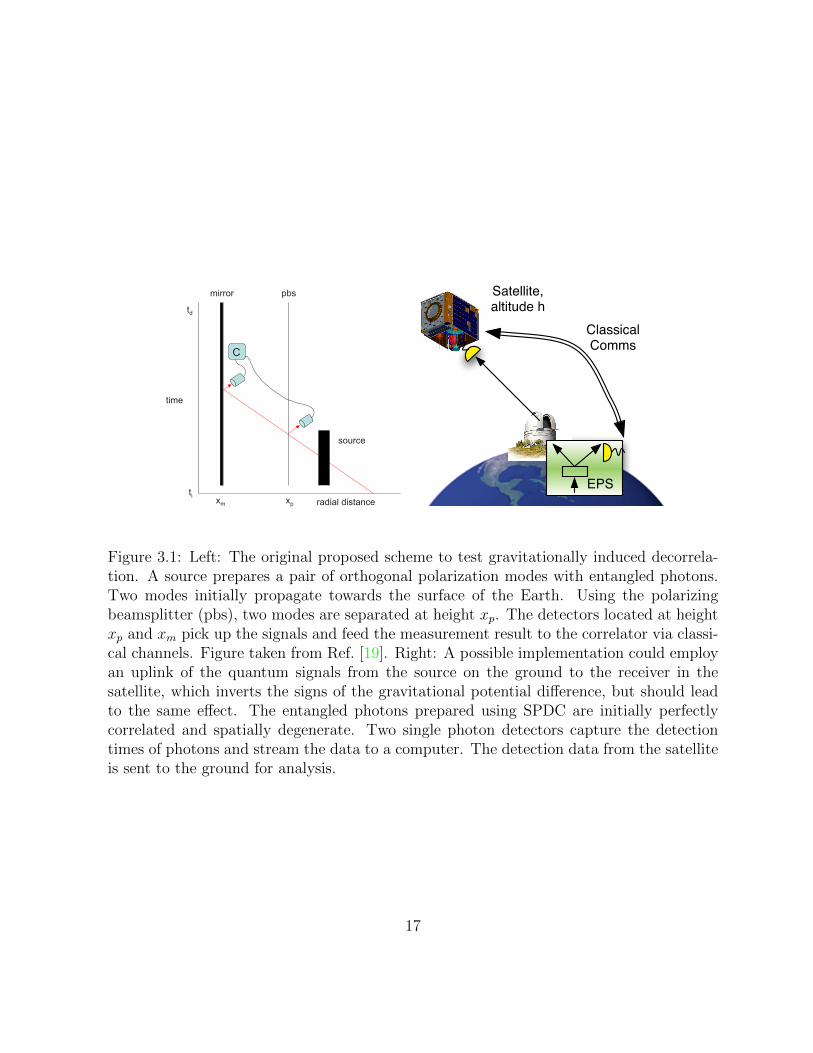
Figure 3.1: Left: The original proposed scheme to test gravitationally induced decorrela-tion. A source prepares a pair of orthogonal polarization modes with entangled photons.Two modes initially propagate towards the surface of the Earth. Using the polarizingbeamsplitter (pbs), two modes are separated at height xp. The detectors located at heightxp and xm pick up the signals and feed the measurement result to the correlator via classi-cal channels. Figure taken from Ref. [19]. Right: A possible implementation could employan uplink of the quantum signals from the source on the ground to the receiver in thesatellite, which inverts the signs of the gravitational potential difference, but should leadto the same effect. The entangled photons prepared using SPDC are initially perfectlycorrelated and spatially degenerate. Two single photon detectors capture the detectiontimes of photons and stream the data to a computer. The detection data from the satelliteis sent to the ground for analysis.
17

dt 2 ps
dt 10 psdt 500 fs
10 100 1000 104 105hkm
0.2
0.4
0.6
0.8
1.0CCmax Coincidence rate vs height of the satellite
LEO GEO
Figure 3.2: Coincidence predictions from the experiment proposed in Ref. [19]. The coin-cidence detection rate (i.e. detection events in both detectors) as a function of temporaldifference of the detection td2− td1 should be peaked around the light traveling time differ-ence in the two “arms”. The maximum coincidence rate C describes the photon correlationupon detection, within the (intrinsic) detection time dt.
where Cmax is the maximum correlation function we should observe in flat spacetime, anddt is the temporal resolution of the photon detectors.
If the photodetector resolution time is 500 fs, then the decoherence should easily beobserved for satellite altitudes above 400 km,1 as illustrated in Figure 3.2. With a GEOsatellite, which orbits at altitude 36,000 km, the effect would be more significant, and evenwith 10 ps response time (the response time of a typical contemporary photodetector), avisible decorrelation effect could occur.
Due to the careful timing required, this scheme is challenging but still possibly doable.It is interesting to note that the predicted decoherence induced by gravity under this alter-native theory applies only to quantum entanglement, and is in addition to any spreadingof classical correlations. Because there are many sources of decoherence for photons trav-eling between satellites and the ground, it will be much easier to refute the event-operatorhypothesis than to confirm it — if we were able to generate entanglement beyond whatis predicted by Eq. 3.6, the hypothesis as proposed would be contradicted. On the other
1This is a conservative estimate compared to the 200 fs quoted in Ref. [19], which would result indecoherence above 90 km.
18

hand, if decoherence were found, it would be difficult to rule out other source of deco-herence, which we may overlooked. If that is the case, one could employ a satellite in anelliptical orbit to perform the test when the satellite is at different heights to see whetherthe decorrelation changes in accord with Eq. 3.6.
Note that an alternative approach to the setup of Figure 3.1 (right panel) is to equipa retroreflecting mirror on the satellite instead of a photon detector. However, one ofthe entangled photon pair would have to travel through the atmosphere twice instead ofjust once, which would cause further loss of photon. It would have the benefit that therequirement of satellite orbit height is halved at which an effect can be seen. The theorywould predict the same curves as in Figure 3.2 but with each tick mark on the horizontalaxis replaced with half its current value. As a trade off between photon loss and satelliteheight requirement, it might be advantageous in certain setups.
19

Chapter 4
Testing envariance
4.1 Introduction
Envariance, or environment - assisted invariance, is a quantum symmetry that discoveredby Zurek in attempt to explain the origin of decoherence [21, 22, 23]. It applies in caseswhere a bipartite quantum state is present. The state consists of a system part, labeledS, and an environment part, labeled E. If some non-trivial action is applied to the systempart only, described by some unitary evolution, US = uS ⊗ IE, then the state is said tobe envariant under US if another unitary applied to the environment, UE = IS ⊗ uE, canrestore the initial state. Mathematically, it can be expressed,
US|ψSE〉 = (uS ⊗ IE)|ψSE〉 = |ψ′SE〉 (4.1)
UE|ψ′SE〉 = (IS ⊗ uE)|ψ′SE〉 = |ψSE〉. (4.2)
Envariance is an example of an assisted symmetry [21] where once the system is transformedunder some unitary US, it can be restored to its original state by another operation ona distinct system: the environment. It is hard to imagine such symmetry in a classicalframework, since non-trivial changes applied to a classical system could be never be restoredby action on a distant classical system.
Envariance is a uniquely quantum symmetry in the following sense. A pure staterepresents complete knowledge of the quantum system. In an pure entangled quantumstate, however, complete knowledge of the whole system does not imply complete knowledgeof its parts. It is therefore possible that an operation on one part of a quantum state canalter the global state, but its local effects are masked by incomplete knowledge of that
20

part; the effect on the global state can then be undone by an action on a different part. Incontrast, complete knowledge of a composite classical system implies complete knowledgeof each of its parts. Thus transforming one part of a classical system cannot be masked byincomplete knowledge and cannot be undone by a change on another part.
Envariance plays a prominent role in work related to fundamental issues of decoher-ence and quantum measurement [21, 22, 23]. Decoherence converts amplitudes in coherentsuperposition states to probabilities in mixtures and is central to the emergence of theclassical world from quantum mechanics [24, 25]. Mathematically the mixture appears inthe reduced density operator of the system which is extracted from the global wavefunctionby a partial trace [26, 27]. This partial trace limits the approach for deriving, as opposed toseparately postulating, the connection between the wavefunction and measurement proba-bilities known as Born rule [28], since the partial trace assumes Born rule is valid [22, 25].Envariance was employed in a derivation of Born rule which sought to avoid circularityinherent to approaches which rely on partial trace [22]. For comments on this derivation,see for example [25].
In the present work, we subject envariance to experimental test in an optical system.We use the polarization of a single photon to encode the system, S, and the polarizationof a second single photon to encode the environment, E. We subject the system photon toa wide range of polarization rotations with the goal of benchmarking the degree to whichwe can restore the initial state by applying a second transformation on the environmentphoton. My contribution for this work was designing the experiment described in section4.3 and putting bounds on the Born rule in section 4.4.
4.2 Deriving Born rule from envariance
Before we go into the experiment, lets give the brief introduction of deriving Born rulefrom envariance. Like other derivation of the Born rule such as Gleason’s theorem, thisderivation follows a number of general assumptions behind quantum mechanics. One couldargue that under the same set of assumptions, Gleason’s theorem should also follow. It isworth pointing out that this derivation is aimed to provide a different perspective at theBorn rule, which is more accessible for people from physics background. Moreover, onemay argue that Gleason’s theorem gives no insight into physical significance of quantumprobabilities, in other word, it is not clear why the observer should assign probabilities inaccord with the measure provided by the Gleason’s approach. This derivation attempts tojustify the quantum definition of probability. In this section, our final goal is to show the
21

Born rule for quantum state |ψSE〉 =∑N
k=1 αk |σk〉 |εk〉. Mathematically, we would like toshow that
Theorem 1. For state in Schmidt form
|ψSE〉 =N∑k=1
αk |σk〉 |εk〉 (4.3)
The probability of measuring |σk〉 in system pk ∝ |αk|2.1
The derivation could be divided into two parts.
First, prove that for |αi|2 = 1N
, pk = 1N
. Then, generalize the result to any rational
|αi|2.
Theorem 2. For state in Schmidt form
|ψSE〉 =N∑k=1
1√Neiθk |σk〉 |εk〉 (4.4)
The probability of measuring |σk〉 in system is pk = 1N∀k ∈ 1, 2, ..., N.
Let’s swap the ith and jth elements in the system. We could do this by swap the labelof those 2 eigenstate without touching any experimental setup. The unitary for the swapcould be written as:
uS = |σi〉 〈σj|+ |σj〉 〈σi|+∑k 6=i,j
|σk〉 〈σk| (4.5)
The state after the swap operation becomes
(uS ⊗ 1) |ψSE〉 =1√Neiθj |σi〉 |εj〉+
1√Neiθi |σj〉 |εi〉
+∑k 6=i,j
1√Neiθk |σk〉 |εk〉 (4.6)
The initial state is envariant under unitary (uS ⊗ 1). One may apply a unitary uE solely onthe environment to recover the original state |ψSE〉. The said unitary uE could be expressedas
uE = ei(θj−θi) |εi〉 〈εj|+ ei(θi−θj) |εi〉 〈εj|+∑k 6=i,j
|εk〉 〈εk| (4.7)
1Born rule for bipartite entangled state
22

We could check that
(uS ⊗ uE) |ψSE〉 =∑k 6=i,j
1√Neiθk |σk〉 |εk〉+
1√Neiθiei(θj−θi) |σj〉 |εj〉
+1√Neiθjei(θi−θj) |σi〉 |εi〉 (4.8)
=∑k
1√Neiθk |σk〉 |εk〉 (4.9)
= |ψSE〉 (4.10)
Before we ask what is the probability of getting outcome |σi〉 and |σj〉 when we measurethe system, we make the following three assumptions.
First, unitary transformations must act on the system to alter its state. Probabilitiesof getting outcome |σi〉 or outcome |σi〉 should not be affected by transformation uE , whichacts only on the environment.
Second, the state of the system S is all that is needed to predict measurement outcomes,including their probabilities.
Finally, the state of a larger composite system that includes S as a subsystem is allthat is needed to determine the state of the system S.
Assume we have probability pi of getting outcome |σi〉 and probability pj of gettingoutcome |σi〉. Since the swap operation only relabels eigenstate i and j, we have
p (i| |ψSE〉) = p (j| (uS ⊗ 1) |ψSE〉) (4.11)
Since operations solely on the environment should not change the measurement outcomein the system, we have
p (j| (uS ⊗ 1) |ψSE〉) = p (j| (uS ⊗ uE) |ψSE〉) (4.12)
After the applying both unitary, we got the original state back, where (uS ⊗ uE) |ψSE〉 =|ψSE〉. Therefore,
p (j| (uS ⊗ uE) |ψSE〉) = p (j| |ψSE〉) (4.13)
Now, from Eq. 4.11, Eq. 4.12 and Eq. 4.13, we conclude that
p (j| |ψSE〉) = p (i| |ψSE〉) (4.14)
23

Due to the freedom of choice of index i and j, the probabilities of measuring any statein this system are the same! Since there are N possible outcomes, and the probabilitiesshould sum up to 1. Thus, the probability of measuring any eigenstate |σk〉 in the systemis pk = 1
N.
We could use the result in Theorem 2 to show Theorem 1. Consider the special examplewhere N = 2.
|ψSE〉 =
√N −M√N
|σl〉 |εl〉+
√M√N|σj〉 |εj〉 (4.15)
Now we put in a large enough ancillary pointer state, and entangle the state with thepointer state.
|ψSE〉 |e0〉 =
√N −M√N
|σl〉S |εl〉E |p0〉P +
√M√N|σj〉S |εj〉E |p1〉P (4.16)
The entangling operation Up is done between the environment and pointer state.
1S ⊗ Up |ψSE〉 |e0〉 =
√N −M√N
|σl〉S |εl〉E |p0〉P +
√M√N|σj〉S |εj〉E |p1〉P (4.17)
Since the ancillary system is large enough, we could rewrite the pointer states in a differentbasis where
|p0〉P =N−M∑k=1
1√N −M
|ηk〉P (4.18)
|p1〉P =N∑
k=N−M+1
1√M|ηk〉P (4.19)
Thus, we could rewrite the state 1S ⊗ Up |ψSE〉 |e0〉 as
1S ⊗ Up |ψSE〉 |e0〉 =
√N −M√N
|σl〉S |εl〉EN−M∑k=1
1√N −M
|ηk〉P
+
√M√N|σj〉S |εj〉E
N∑k=N−M+1
1√M|ηk〉P
=N−M∑k=1
1√N|σl〉S |εl〉E |ηk〉P
+N∑
k=N−M+1
1√N|σj〉S |εj〉E |ηk〉P (4.20)
24
Now we can use Theorem. 2, where the probability of measuring each |ηk〉P should be thesame. In other words,
P (|ηk〉P |1S ⊗ Up |ψSE〉 |e0〉) =1
N. (4.21)
Thus, the probability of detect |σl〉S in system and |ηk〉P in the pointer where k ∈ [1, N−M ]is N−M
N. The probability of detect |σj〉S in system and |ηk〉P in the pointer where k ∈
[N −M + 1, N ] is MN
.
The probability of measuring |σj〉S in the system given state 1S⊗Up |ψSE〉 |e0〉 should beMN
. Since the transformation Up does not act on the system, the probability of measuring|σj〉S in the system given state |ψSE〉 |e0〉 is M
N. This proof could be easily extended to any
N > 2, which prove the Theorem 1. Therefore, we have shown that with a few assumptions,we could derive Born rule from envariance.
4.3 Experimental testing envariance
The derivation presented in Section. 4.2 could be divided into 2 parts. The first part isthe core idea of the derivation, which relates the symmetry to probability of measurementoutcomes. It also requires less resources, where only a two-qubit system is needed. Testingthe second part is more difficult, and the proposal is listed in Appendix A, where a minimumof 4 qubits is needed. In this section, the first part of the derivation is tested.
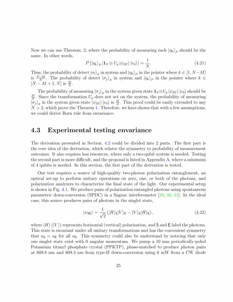
Our test requires a source of high-quality two-photon polarization entanglement, anoptical set-up to perform unitary operations on zero, one, or both of the photons, andpolarization analyzers to characterize the final state of the light. Our experimental setupis shown in Fig. 4.1. We produce pairs of polarization-entangled photons using spontaneousparametric down-conversion (SPDC) in a Sagnac interferometer [29, 30, 31]. In the idealcase, this source produces pairs of photons in the singlet state,
|ψSE〉 =1√2
(|H〉S|V 〉E − |V 〉S|H〉E) , (4.22)
where |H〉 (|V 〉) represents horizontal (vertical) polarization, and S and E label the photons.This state is envariant under all unitary transformations and has the convenient symmetrythat uS = uE for all uS. This symmetry could also be understand by noticing that onlyone singlet state exist with 0 angular momentum. We pump a 10 mm periodically-poledPotassium titanyl phosphate crystal (PPKTP), phase-matched to produce photon pairsat 809.8 nm and 809.3 nm from type-II down-conversion using 6 mW from a CW diode
25

Figure 4.1: Experimental setup. The entangled photon pairs are created using type-IIspontaneous parametric down-conversion. The pump laser is focused on a periodically-poled KTP crystal and pairs of entangled photons with anti-correlated polarizations areemitted. The pump is filtered using a band-pass filter, and polarization controls adjustfor the alterations due to the coupling fibers. The entangled photon pairs are set so onephoton is considered the system, and the other is considered the environment. After thesource the unitary transformations are applied. A three wave plate combination is requiredto apply an arbitrary unitary transformation: quarter wave-plate (QWP), half wave-plate(HWP), QWP. A set of this combination of wave plates is mounted on each translationstage which can slide the wave plates in and out of the path of the incoming photons. Thephotons are then detected using polarizing beam splitters (PBS) and two wave plates totake projective measurements. The counts measured using avalanche photodiode (APD)are then analyzed using coincidence logic.
26
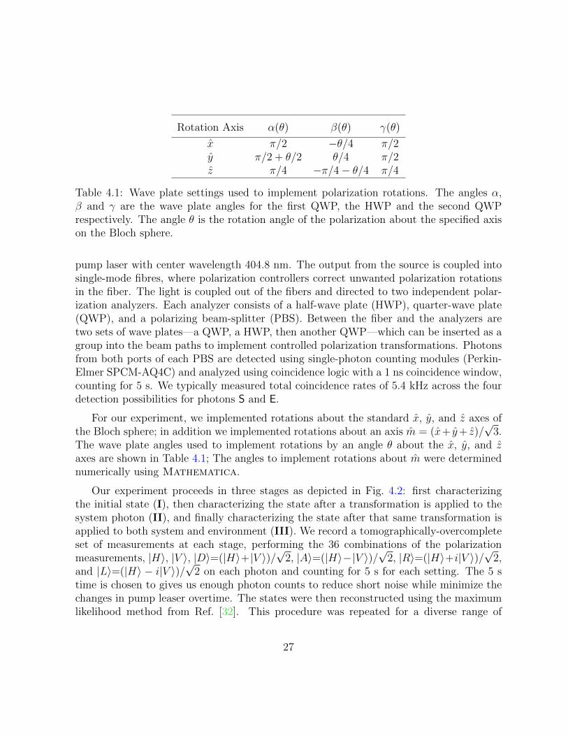
Rotation Axis α(θ) β(θ) γ(θ)
x π/2 −θ/4 π/2y π/2 + θ/2 θ/4 π/2z π/4 −π/4− θ/4 π/4
Table 4.1: Wave plate settings used to implement polarization rotations. The angles α,β and γ are the wave plate angles for the first QWP, the HWP and the second QWPrespectively. The angle θ is the rotation angle of the polarization about the specified axison the Bloch sphere.
pump laser with center wavelength 404.8 nm. The output from the source is coupled intosingle-mode fibres, where polarization controllers correct unwanted polarization rotationsin the fiber. The light is coupled out of the fibers and directed to two independent polar-ization analyzers. Each analyzer consists of a half-wave plate (HWP), quarter-wave plate(QWP), and a polarizing beam-splitter (PBS). Between the fiber and the analyzers aretwo sets of wave plates—a QWP, a HWP, then another QWP—which can be inserted as agroup into the beam paths to implement controlled polarization transformations. Photonsfrom both ports of each PBS are detected using single-photon counting modules (Perkin-Elmer SPCM-AQ4C) and analyzed using coincidence logic with a 1 ns coincidence window,counting for 5 s. We typically measured total coincidence rates of 5.4 kHz across the fourdetection possibilities for photons S and E.
For our experiment, we implemented rotations about the standard x, y, and z axes ofthe Bloch sphere; in addition we implemented rotations about an axis m = (x+ y+ z)/
√3.
The wave plate angles used to implement rotations by an angle θ about the x, y, and zaxes are shown in Table 4.1; The angles to implement rotations about m were determinednumerically using Mathematica.
Our experiment proceeds in three stages as depicted in Fig. 4.2: first characterizingthe initial state (I), then characterizing the state after a transformation is applied to thesystem photon (II), and finally characterizing the state after that same transformation isapplied to both system and environment (III). We record a tomographically-overcompleteset of measurements at each stage, performing the 36 combinations of the polarizationmeasurements, |H〉, |V 〉, |D〉=(|H〉+|V 〉)/
√2, |A〉=(|H〉−|V 〉)/
√2, |R〉=(|H〉+i|V 〉)/
√2,
and |L〉=(|H〉 − i|V 〉)/√
2 on each photon and counting for 5 s for each setting. The 5 stime is chosen to gives us enough photon counts to reduce short noise while minimize thechanges in pump leaser overtime. The states were then reconstructed using the maximumlikelihood method from Ref. [32]. This procedure was repeated for a diverse range of
27

Figure 4.2: Experimental measurement procedure. We investigated the impact of eachunitary transformation by performing quantum state tomography at three different stages:directly on the initial state with no unitary transformations (I), on the state with a trans-formation applied to the system photon (II), and on a state with the same transformationapplied to both the system and environment photon (III).
transformations. We configured our setup to implement unitary rotations in multiples of30 from 0 to 360 about each of the x, y, z, and m axes. The data acquisition time forthis procedure over the set of 13 rotation angles about each axis was approximately sixhours. The source was realigned before each set of rotations to achieve maximum fidelitywith the singlet state from 0.985 to 0.990.
Figure 4.3a)–c) show the real and imaginary parts of the reconstructed density matrixof the quantum state at the three stages in the experiment, I, II, and III respectively. Thefidelity [33] of the state with the ideal |ψ−〉 state during these samples of two of the stagesare 0.987 for both I, and III, respectively, and is defined as [33]:
F (ρ, σ) = Tr[(√ρσ√ρ)1/2]2
(4.23)
We can use this definition to calculate the fidelity between the state at stages I and III.Comparing between the states shown in Fig. 4.3 panels a) and c) the resulting fidelity is0.995.
The summary of the results from our experiment is shown in Fig. 4.4. The coloureddata points in Fig. 4.4a)–d) show the fidelity of the experimentally reconstructed stateat stage III with the reconstructed state from the initial stage I, i.e., F (ρIexpt, ρ
IIIexpt), as a
function of the rotation angle for rotations about the x, y, z, and m, respectively. Theopen circles show the theoretical expectation for the fidelity between the measured stateat stage I with the expected state in stage III, calculated by acting the unitaries on themeasured state from stage I, i.e., F (ρIexpt, ρ
IIIth ). The fidelities are very high, close to the
limit of 1, in all cases and we see reasonable agreement with expectation.
28

Figure 4.3: a) The real and imaginary parts of the reconstructed density matrix of theinitial state from the source (stage I of the procedure). It has 0.987 fidelity [33] with theideal. b) The system photon is transformed using wave plates set to implement the rotationof 90 about the x axis, stage II. The resulting density matrix shown has 0.488 fidelity withthe ideal initial state,0.501 with the initial reconstructed state and 0.995 with the expectedstate, calculated by transforming the density matrix from a). c) The reconstructed densitymatrix after the same unitary from b) is applied to both photons, stage III. This state hasa 0.987 fidelity with the ideal, 0.995 with the reconstructed state from a), and 0.997 withthe expected state calculated by transforming the state from part a).
We considered the effects of Poissonian noise, which describes the fluctuations of thenumber of photons detected, and waveplate calibration on our results and found that theseeffects were too small to explain the deviation between F (ρIexpt, ρ
IIIexpt) and F (ρIexpt, ρ
IIIth ).
To account for this, we characterized the fluctuations in the state produced by the sourceitself by comparing the state produced in subsequent stage I sates in the data collection;recall that stage I for each choice of unitary is always the same (no additional waveplates
29

0 6 0 1 2 0 1 8 0 2 4 0 3 0 00 . 9 8 0
0 . 9 8 5
0 . 9 9 0
0 . 9 9 5
1 . 0 0 0
0 6 0 1 2 0 1 8 0 2 4 0 3 0 0 0 6 0 1 2 0 1 8 0 2 4 0 3 0 0 0 6 0 1 2 0 1 8 0 2 4 0 3 0 0
0 6 0 1 2 0 1 8 0 2 4 0 3 0 00 . 9 9 8 0
0 . 9 9 8 5
0 . 9 9 9 0
0 . 9 9 9 5
1 . 0 0 0 0
0 6 0 1 2 0 1 8 0 2 4 0 3 0 0 0 6 0 1 2 0 1 8 0 2 4 0 3 0 0 0 6 0 1 2 0 1 8 0 2 4 0 3 0 0Bhatt
acha
ryya C
oeffic
ient a )
x y z m
b ) c )
e ) g )f )
d )
R o t a t i o n A n g l e ( D e g r e e s )
Fidelit
y
h )
Figure 4.4: Analysis of the experimental results. Panels a)–d) show the fidelity analysisresults for unitary rotations about x, y, z, and m axes as functions of rotation angle. Thecoloured data points are the comparison between stage I and stage III (comparing thesource state and the state after the unitary has been applied to both qubits). The opencircles show a theoretical comparison. Panels e)–h) show the quantum Bhattacharyyaresults comparing stage I and stage III in the coloured data points for each of the fouraxis, with the open circles being the theoretical comparison. For plots which include acomparison of stage I and II (applying the unitary to one qubit only) and theoreticalcomparisons, see the appendix. The error bar for each graph is the standard deviation ofcomparisons of source state measurements during the experiment.
30

Rotation Axis Average Fidelity Average BC
x 0.997± 0.001 0.9997± 0.0001y 0.9973± 0.0007 0.99966± 0.00008z 0.9984± 0.0006 0.99975± 0.00007m 0.9941± 0.0007 0.9994± 0.0001
Overall average: 0.9966± 0.0004 0.99963± 0.00005
Table 4.2: Summary of the results for comparing stages I and III using fidelity and Bhat-tacharyya Coefficient (BC) analysis and averaging over each unitary rotation. The overallaverage is representative of the overall envariance of our state.
inserted) and thus provides a good measure of the source stability. Specifically, we cal-culated the standard deviation in the fidelity of the state produce at a stage I in the ith
round of the experiment to that produced in the next, (i + 1)th, stage I, F (ρI,iexpt, ρI,i+1expt ).
The standard deviation in these fidelities calculated from the data taken within each setof rotation axes are shown as representative error bars on the plots in Figs. 4.4a)–d). Thestandard deviation of this quantity over all the experiments was 0.0008. We characterizethe difference between the measured and expected fidelities by calculating the standarddeviation in the quantity, F (ρIexpt, ρ
IIIexpt)− F (ρIexpt, ρ
IIIth ), for each experiment. (This is the
difference between the coloured and open data points in Figs. 4.4a)–d).) over all exper-iments to be 0.002. This value is comparable to the error in the fidelity due to sourcefluctuations. Refer to the appendix to see the comparison between stage I and stage II,which would not fit on the scale of Fig. 4.4.
From our data, we extract the average fidelity F (ρIexpt, ρIIIexpt) for the set of measurements
made for each unitary axis and show the results in Table II. As measured by the averagefidelity, our experiment benchmarks envariance to 0.9966± 0.0004,((99.66± 0.04)% of theideal) averaged over all rotations.
Fidelity has conceptual problems as a measure for testing quantum mechanics, since thedensity matrix we used to compute the fidelity is reconstructed using state tomography,which is under the assumption of Born rule. The Bhattacharyya Coefficient (BC) is ameasure of the overlap between two discrete distributions P and Q, where pi and qi arethe probabilities of the ith element for P and Q respectively. The BC is defined [34],
BC =∑i
√piqi. (4.24)
If we normalize the measured tomographic data by dividing by the sum of the counts,we can treat this as a probability distribution. The BC then can be calculated using the
31

distribution of measurements at each stage in the experiment, directly analogous to theapproach used with fidelity. It should be noted that the BC has some limitations whenapplied in this case. If two quantum states produce identical measurement outcomes, itsvalue is 1. Unlike fidelity though, it is not the case that the BC goes to 0 for orthogonalquantum states. For example, the BC for two orthogonal Bell states measured with anovercomplete set of polarization measurements is 7/9. Furthermore, the value of the BCis dependent on the particular choice of measurements taken. While we are employing acommonly-used measurement set for characterizing two qubits, other choices would producedifferent BCs. Nevertheless, this metric can be employed to quantify the envariance in ourexperiment without quantum assumptions, making it appropriate for testing quantummechanics.
The Bhattacharyya Coefficients from our measured data are shown in Fig. 4.4e)–h). Wenormalize the measured counts from stages I and III to give us probability distributionspIexpt and pIIIexpt. The coloured data points in Figs. 4.4e)–h) show the BC between thesedistributions, BC(pIexpt, p
IIIexpt). The open circles are a theoretical expectation of the BC
given the tomographic measurements from stage I; for these theoretical values we used statetomography, and thus assumed quantum mechanics, to obtain the expected distributionpIIIth and calculate the expected BC, BC(pIexpt, p
IIIth ).
Using an analogous procedure to that employed with the fidelity, we estimate the un-certainty in the BC by comparing subsequent measured distributions in stage I throughoutthe experiment, i.e., BC(pI,iexpt, p
I,i+1expt ). A representative error bar calculated from the data
for a set of unitaries around the same axis are shown in Fig. 4.4e)–h). The standarddeviation in this quantity over all the data is 0.00005. As before we characterize the dif-ference between the measured and expected BCs as the standard deviation of the quantityBC(pIexpt, p
IIIexpt) − BC(pIexpt, p
IIIth ) which is 0.00009 over all experiments. As before, this
value is comparable to the error due to source fluctuations. Data showing the BC betweenstage I and II are shown in the appendix along with analogous theoretical comparison.A summary of the BC analysis results are in Table 4.2. The average measured BC is0.99963± 0.00005 ((99.963± 0.005)% of the ideal) across all tested unitaries.
4.4 Bounds to Born rule
In our experiment, we place a bound on the degree of envariance. It has been shownthat envariance can be used to derive Born rule [23, 28]. However, the derivation does notrelate bounds on Born rule to bound on envariance. In order to do so, we explore a recentlyproposed extension of quantum mechanics by Son [1]. Son’s theory generalizes Born rule,
32

replacing the familiar power of 2 which relates wavefunctions to probabilities with a powerof n. In this section, we summarize Son’s theory and use it to put a bound on n using ourexperimental data.
We first consider measurements on a pair of qubits in the maximally entangled singletstate using standard quantum mechanics. We define measurement observables a = ~α · ~σ1
and b = ~β · ~σ2 where ~α, ~β are unit vectors and ~σ1, ~σ2 are the Pauli matrices for the twoqubits. The result of measurements a and b for qubits 1 and 2 respectively can take on thevalues ±1. The correlation function is defined by
E = 〈ab〉 = Pa=b − Pa6=b, (4.25)
where Pa=b and Pa6=b are probabilities that a = b and a 6= b respectively. The correlation
function only depends on the angle 2θ between ~α and ~β for the singlet state. From Bornrule, we have the probability amplitudes ψa=b and ψa6=b satisfy Pa=b = |ψa=b|2 and Pa6=b =|ψa6=b|2. Therefore, the correlation function in standard quantum mechanics is given by
EQM(θ) = |ψa=b|2 − |ψa6=b|2 = − cos 2θ. (4.26)
We now consider Son’s theory, where Born rule is generalized to be Pa=b = |ψa=b|n andPa6=b = |ψa6=b|n, and the correlation function is thus,
E(θ, n) = |ψa=b|n − |ψa6=b|n, (4.27)
where standard quantum mechanics is the special case E(θ, 2) = EQM(θ). As in standardquantum mechanics, Son assumed that the correlation function depends only on the anglebetween measurement settings. Son showed that the constraints |∂ψa=b
∂θ|2 + |∂ψa 6=b
∂θ|2 ∝ 1
and |ψa=b|n + |ψa6=b|n = 1 and the boundary condition E(0, n) = −1 and E(π2, n) = 1 are
sufficient to solve for E(θ, n). See [1] for further details on the deviation. Figure 4.5 showsE(θ, n) for different value n.
In the experiment, we rotated one qubit while leaving the other qubit unchanged dur-ing the stage II (See Figure 4.2) . If we use the same measurement basis on both qubitsfor that rotated state, we are effectively measuring the singlet state input with two mea-surement basis with angle θ apart. For example, we can choose the rotation axis and themeasurement basis to be [Z,(D,A)], where the first qubit is rotated around Z axis, whilemeasurements on the qubits are done in (D,A) basis. Since the rotation axis Z is orthogo-nal to the measurement basis (D,A), we could view the rotation of qubit as a rotation ofthe measurement basis in the D-A plane. For a rotation angle φ, the angle between twomeasurement basis is given by 2θ = π − |π − 2φ|. We could derive prediction of E(φ, n)from Son’s theory, and test it with our data.
33
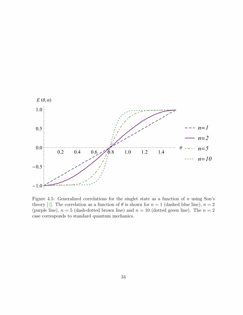
0.2 0.4 0.6 0.8 1.0 1.2 1.4 q
-1.0
-0.5
0.0
0.5
1.0E Hq, nL
n=1n=2n=5n=10
Figure 4.5: Generalized correlations for the singlet state as a function of n using Son’stheory [1]. The correlation as a function of θ is shown for n = 1 (dashed blue line), n = 2(purple line), n = 5 (dash-dotted brown line) and n = 10 (dotted green line). The n = 2case corresponds to standard quantum mechanics.
34

Son’s derivation assumes a perfect singlet state which must be relaxed to obtain acomparison with experiment. For a realistic state, the correlation function will not nec-essarily depend only on θ. In his derivation, Son additionally assumed E(0, n) = −1and E(π/2, n) = 1, i.e., perfect correlations, which are not experimentally achievable. Torelax these assumptions, we consider the difference between two correlation functions mea-sured for a general state ρ and the ideal state |ψ−〉, E(φ, n, ρ) and E(φ, n, |ψ−〉) whereφ is the rotation angle of one of the settings. For n ≈ 2, we make the assumption thatE(φ, n, ρ) − E(φ, n, |ψ−〉) ≈ E(φ, 2, ρ) − E(φ, 2, |ψ−〉). Thus for states close to the idealsinglet state and for n close to 2, we have the relation:
E(φ, n, ρ) ≈ E(φ, n, |ψ−〉) + E(φ, 2, ρ)− E(φ, 2, |ψ−〉). (4.28)
We calculated E(φ, 2, ρ) and E(φ, 2, |ψ−〉) from standard quantum mechanics, and useSon’s theory to calculate E(φ, n, |ψ−〉). For a given set of data Eexp(φi), we find ρ andn to minimize the objective function L = Σi[E(φi, n, ρ) − Eexp(φi)]
2/[δEexp(φi)]2, where
δEexp(φi) is the standard deviation of correlation function Eexp(φi) predicted assumingPoissonian count statistics. Figure 4.6 shows the results of fitting the correlation functionsfor 6 sets of data. From this, we extracted n = 2.04, 2.01, 2.00, 2.01, 2.01, 2.00; averagingthese results and using their standard deviation to estimate the uncertainty yields n =2.01± 0.02 in good agreement with Born rule where n = 2.
4.5 Conclusion
Our deviation from perfect envariance can be understood from our initial state fidelity.However, we also consider the magnitude of the violation of Born rule if one instead assumesall of the deviation stems from such a violation. One recently proposed extension of Bornrule [1] determines probabilities by raising the wavefunction to the power of n rather thanBorn rule which raises the wavefunction to the power of 2. In this theory, the correlationbetween measurement outcomes as a function of measurement setting on a singlet statedepends on the power of n, thus we can test this theory using our experimental data.Fitting our experimental data to this model, we find n = 2.01 ± 0.02 in good agreementwith Born rule.
We have experimentally tested the property of envariance on an entangled two-qubitquantum state. Over a wide range of unitary transformations, we experimentally showedenvariance at (99.66±0.04)% when measured using the fidelity and (99.963±0.005)% usingthe Bhattacharyya Coefficient. Deviations from perfect envariance are in good agreement
35

ññ
ñ
ñ
ñ
ññ
ñ
ñ
ñ
ñ
ññì
ì
ì
ì
ì
ìì
ì
ì
ì
ì
ììò
ò
ò
ò
ò
ò
òò
ò
ò
ò
ò
òõõ
õ
õ
õ
õ
õõ
õ
õ
õ
õ
õç ç
ç
ç
ç
ç
çç
ç
ç
ç
ç
çà à
à
à
à
à
à à
à
à
à
à
à
0.5 1.0 1.5 2.0 2.5 3.0f
-1.0
-0.5
0.0
0.5
1.0
E HfL
Figure 4.6: Correlation functions versus the rotation angle φ. The experimental correla-tions are extracted from our data for the case where the rotation axis and the measurementbasis are given by [Z,(D,A)], [Z,(R,L)], [Y,(D,A)], [Y,(H,V)], [X,(R,L)], [X,(H,V)] shownas red squares, blue circles, green up triangles, yellow down triangles, black empty squares,pink diamonds as a function of the rotation angle φ. The best fit using Eq. 4.28 for eachcorrelation is shown as a line whose colour matches the corresponding data points. Thesefits yield estimates for the value of n of 2.04, 2.01, 2.00, 2.01, 2.01, 2.00, respectively.
36
with theory and can be explained by our initial state fidelity and fluctuations in the proper-ties of our state. Fitting our results to a recently published model which does not explictlyassume Born rule yields nevertheless good agreement with it. Our results serve as a bench-mark for the property of envariance, as improving the envariance of the state significantlywould require substantive improvements in source fidelity and stability. It would be in-teresting to extend tests of envariance to higher dimensional quantum state and to otherphysical implementations.
37

Chapter 5
Pure State Tomography using PauliObservables
5.1 Introduction
Quantum state tomography is one of the essential tasks in quantum information. It is veryexpensive since the required resources grow exponentially with the number of qubits.
What is the task of quantum state tomography? Mathematically, let us consider ad-dimensional Hilbert space Hd, and denote D(Hd) the set of density operators acting onHd. We then measure a set of m linearly independent observables
A = (A0, A1, A2, . . . , Am−1), (5.1)
where each Ai is Hermitian. Without loss of generality, we assume A0 = I (i.e. the identityoperator on Hd), and trAi = 0 for i = 1, 2, . . . ,m− 1.
For any ρ ∈ D(Hd), the Born rule tells us that the measurement returns a set ofoutcomes
α = (tr ρ, tr(ρA1), tr(ρA2), . . . , tr(ρAm−1)). (5.2)
Since ρ ∈ D(Hd), we should theoretically always have tr ρ = 1. However we keep this entryin α for the reason of experimental calibration [35, 36, 37, 38].
For an arbitrary ρ ∈ D(Hd), full quantum state tomography requires order d2 measure-ment outcomes to determine ρ [39]. However for a pure state |ψ〉 ∈ Hd, in general onlyorder d measurements are needed to determine |ψ〉. It could be by chose any orthonormal
38

base to expand the pure state |ψ〉, where only d complex numbers are required to uniquelydetermine this expansion. By measuring the amplitude of |ψ〉 projected onto each basisstate and their relative phase, pure state |ψ〉 can be determined with 2(d − 1) measure-
ments. For a general mixed state, one would need to determine d(d−1)2
elements of thedensity matrix to uniquely determine the quantum state. For a pure state, one could useonly order d parameters to describe the state. An ideal protocol should only require orderd measurements.
In literature, people has come up with two slight different ways in interpreting the term‘determine’, as clarified in a recently paper [40] and could be summarized in the followingdefinition.
Definition 1. A pure state |ψ〉 is uniquely determined among pure states (UDP) bymeasuring A if there does not exist any other pure state which has the same measurementresults as those of |ψ〉 when measuring A. A pure state |ψ〉 is uniquely determined amongall states (UDA) by measuring A if there does not exist any other state, pure or mixed,which has the same measurement results as those of |ψ〉 when measuring A.
The physical interpretation in this case is clear: it is useful in quantum tomography tohave some prior knowledge that the state to be reconstructed is pure or nearly pure. It isknown that there exists a family of 4d−5 observables such that any d-dimensional pure stateis UDP [41], and 5d−6 observables such that any d-dimensional pure state is UDA [40]. Afew other methods for pure-state tomography have also been theorized, and experimentallytested to demonstrate the drop of the number of measurements needed [42, 43, 44, 45, 46,47, 48, 49]. However, even if there are constructive protocols for the measurement set A,in practice these sets may not be easy to measure in an experiment.
One idea of the compressed sensing protocols as discussed in [50, 51] considers measure-ments of Pauli operators for n-qubit systems, with Hilbert space dimension d = 2n. Sinceno joint measurements on multiple qubits are needed for Pauli operators, these operatorsare relatively easy to measure in practice. It is shown that order d log d random Paulimeasurements are sufficient to UDA almost all pure states [52]. That is, all pure statescan be determined, up to a set of states with measure zero (i.e. ‘almost all’ pure states aredetermined). Experiments also demonstrate the usefulness of this method in pure-statetomography in practice [53]. However, it remains open how many Pauli measurements areneeded to determine all pure states (UDP or UDA) of an n-qubit system.
In this work, we examine the problem of the minimum number of Pauli operators neededto UDA all n-qubit pure states. For n = 1 the number is known to be 3, i.e. all three Paulioperators X, Y, Z are needed. We solve the problem for n = 2 and n = 3, where at least 11
39

Pauli operators are needed for n = 2 and at least 31 Pauli operators are needed for n = 3.We then demonstrate that our protocol is robust under depolarizing error with simulatedrandom pure states. We further implement our protocol in our nuclear magnetic resonance(NMR) system and compare our result with other methods. As a direct application of thisresult, we show that our scheme can also be used to reduce the number of settings neededfor pure-state tomography in quantum optical system. My contribution in this work isfinding the optimum Pauli set for 2 qubit pure state tomography in section 5.3, proposedtest in NMR then process the experimental result and analysis the robustness in section5.5, and at last generalize the result to optics in section 5.6.
5.2 Historical results on UDP and UDA
In this work we consider two different kinds of “unique determinedness” for |ψ〉:
1. We say |ψ〉 is uniquely determined among pure states (UDP) by measuring A if theredoes not exist any other pure state which has the same measurement results as thoseof |ψ〉 when measuring A.
2. We say |ψ〉 is uniquely determined among all states (UDA) by measuring A if theredoes not exist any other state, pure or mixed, which has the same measurementresults as those of |ψ〉 when measuring A.
It is known that there exists a group of 4d−5 observables, under which any pure state isUDP, in contrast to the d2−1 observables in the standard method of quantum tomographyfor arbitrary state [41]. Therefore, we can safely say that it is useful for the purpose ofquantum state tomography to have the prior knowledge that the state to be reconstructedis pure or nearly pure.
When the state is UDP, to make the result useful, one needs to verify that the stateis indeed pure. This is not in general practical. One solution to that would be readilygeneralize the above mentioned UDP results to low rank states, where the physical con-straints (e.g., low temperature, locality of interaction etc.) may ensure that the actualphysical state (which ideally supposed to be pure) is indeed low rank. Alternatively, if thestate is UDA, however, in terms of tomography one does not need to bother with thesephysical assumptions, because in the event there is only a unique state compatible withthe measurement results, which turns out to be pure (or low rank).
40

There is also another clear physical intuition for the states that are UDA by measuringobservables from A. Let us consider a Hamiltonian of the form
HA =m∑i=1
αiAi. (5.3)
We observe that any unique ground state |ψ〉 of HA is UDA by measuring A. It is easyto verify: if there is any other state ρ that gives the same measurement results, then ρhas the same energy as that of |ψ〉, which is the ground state energy. Therefore, any purestate in the range of ρ must also be a ground state, which contradicts the fact that |ψ〉is the unique ground state. In other words, UDA is a necessary condition for |ψ〉 to bea unique ground state of HA. It is in general not sufficient, but the exceptions are likelyrare [54, 55].
5.3 2 qubit pure state tomography using Paulis mea-
surements
We define the single-qubit Pauli operators by σ1 = X, σ2 = Y, σ3 = Z, and the identityoperator σ0 = I. For a single qubit, it is straightforward to check that measuring only twoof the three operators cannot determine an arbitrary pure state.1 Therefore all three Paulioperators are needed in the single-qubit case.
For the two-qubit system, there are a total of 16 Pauli operators, including the identity.These are given by the set σi⊗σj with i, j = 0, 1, 2, 3. For simplicity we omit the tensorproduct symbol by writing, e.g. XY instead of X ⊗ Y . Of these 16 Pauli operators, thereexists a set of 11 Pauli operators A such that A is UDA for any pure state, as given bythe following theorem [56].
Theorem 3. Any two-qubit pure state |φ〉 is UDA by measuring the following set of Paulioperators.
A = II, IX, IY, IZ,XI, Y X,Y Y, Y Z, ZX,ZY, ZZ, (5.4)
1Some state can still be determined using only two of the three operators. For example, any state12 (I + αX + βY ), where α2 + β2 = 1 could be determined without measuring observable Z
41

and no set with fewer than 11 Pauli operators can be UDA for all two-qubit pure states.Moreover, any set of Pauli operators which is Clifford equivalent to A is UDA for anytwo-qubit pure states.
This is to say, 11 is the minimum number of Pauli operators needed to UDA anytwo-qubit pure state, and an example of such a set with 11 Pauli operators is given inEq. (5.4).
Proof. In order for A to UDA all two-qubit pure states it is known [40] that any Hermitianoperator H ∈ (S(A))⊥ must have at least two positive and two negative eigenvalues, whereS(A) means the linear span of A.
In this case (S(A))⊥ = S(XX,XY,XZ, Y I, ZI). Note that the 5 operators which arenot measured all mutually anti-commute with each other. It is easy to see that this propertyis required for if two operators in (S(A))⊥ commuted, then they would be simultaneouslydiagonalizable and a linear combination would exist which would have at least one 0-eigenvalue. Since two-qubit Pauli operators only have four eigenvalues total, having asingle 0 eigenvalue fails the UDA condition.
Furthermore it is easy to show by exhaustive search that there exists no set of morethan 5 mutually anti-commuting Pauli operators. So no fewer than 11 Paulis could bemeasured.
To show that this set of 11 Pauli operators is sufficient to be UDA, we construct aparametrization of all H ∈ (S(A))⊥;
H = α1XX + α2XY + α3XZ + α4Y I + α5ZI (5.5)
and show that either H has two positive and two negative eigenvalues or H = 0. Note thatH then has the following form:
α5 0 α3 + α4i α1 + α2i0 α5 α1 − α2i −α3 + α4i
α3 − α4i α1 + α2i −α5 0α1 − α2i −α3 − α4i 0 −α5
.The determinant of H can be calculated and the result is:
α45 + α2
5|α3 + α2i|2 + α25|α1 + α2i|2
+ |α3 − α4i|4 + |α3 − α4i|2|α1 + α2i|2 + |α3 − α2i|2α25
+ |α1 − α2i|4 + |α1 − α2i|2|α3 − α4i|2 + |α1 − α2i|2α25.
42

This quantity, being the sum of non-negative terms, is greater than or equal to 0.Equality is reached if and only if all terms in the sum are 0, which only occurs whenα1 = α2 = α3 = α4 = α5 = 0. Since H is a 4-by-4 traceless Hermitian matrix, it canonly have positive determinant if and only if it has exactly two positive and two negativeeigenvalues.
The same logic follows for any set that is unitarily equivalent to this set. A particularclass of unitary operators which maps the set of Pauli operators to itself is called the Cliffordgroup. Thus, the set A in Eq. 5.4 and any set which is Clifford equivalent [57] to it are ouroptimum sets of Pauli measurement operators for two-qubit pure-state tomography.
5.4 3 qubit pure state tomography using Paulis mea-
surements
The situation for the 3-qubit case is much more complicated [56]. We start by noticingthat
V = IIZ + IZI + ZII + ZZZ
= 4 (|000〉〈000| − |111〉〈111|) (5.6)
has one positive and one negative eigenvalue. Therefore, if the set F1 = IIZ, IZI, ZII, ZZZis a subset of S(A)⊥, the set A cannot UDA all pure states. Similarly any set Fi which isClifford equivalent to F1 cannot be a subset of S(A)⊥. Sets such as these we call failingsets.
Definition 2. A failing set F is a set of Pauli operators such that there exists a nonzeroreal combination of elements chosen from F such that it has only 1 positive eigenvalue or1 negative eigenvalue.
Namely, for an arbitrary pure state |φ〉 to be UDA by measuring operators in a set A,span(Fi) 6⊂ (span(A))⊥ holds for every set Fi that is Clifford equivalent to F1. Thus, forall 945 sets of Fi, at least one element in each Fi should be included in span(A).
Theorem 4. The following set of 31 Pauli operators are sufficient to UDA any given
43

three-qubit pure state |φ〉
A = IIX, IIY, IIZ, IXI, IXX, IXY, IY I, IY X,IY Y, IZI,XIZ,XXX,XXY,XY X,XY Y,
XZX,XZY, Y XX, Y XY, Y XZ, Y Y X, Y Y Y,
Y Y Z, Y ZI, ZII, ZXZ,ZY Z,ZZX,ZZY,
ZZZ, III, (5.7)
and no set with less than 31 Pauli operators can be UDA for all three-qubit pure states.Moreover, any set of Pauli operators which is Clifford equivalent to A can be used to UDAfor any three-qubit pure states.
Similarly to the two-qubit case this set is obtained by finding the largest set of Paulioperators which do not contain any of the identified failing sets and taking the complementproducing the smallest set of measurement operators which could UDA all pure states.
To show that this set A will be UDA for any pure state, we look at the tracelessHermitian operator H ∈ (span(A))⊥, where
H = α1IXZ + α2IY Z + α3IZX + α4IZY + α5IZZ
+α6XII + α7XIX + α8XIY + α9XXI
+α10XXZ + α11XY I + α12XY Z + α13XZI
+α14XZZ + α15Y II + α16Y IX + α17Y IY
+α18Y IZ + α19Y XI + α20Y Y I + α21Y ZX
+α22Y ZY + α23Y ZZ + α24ZIX + α25ZIY
+α26ZIZ + α27ZXI + α28ZXX + α29ZXY
+α30ZY I + α31ZY X + α32ZY Y + α33ZZI.
It can be shown that H either has at least two positive and two negative eigenvaluesor H = 0 (see Appendix B for details). Therefore, set A in Eq. 5.7 and any set which isClifford equivalent to it are our optimum Pauli measurement sets for 3-qubit pure-statetomography.
44

5.5 Pure state tomography in NMR system
A nuclear magnetic resonance (NMR) system is an ideal testbed for our protocol. However,the creation of a pure state in NMR requires unrealistic experimental conditions such asextremely low temperatures or high magnetic fields, which makes it impractical for a liquidsample. To overcome this problem, one can prepare a pseudo-pure state (PPS) alternatively
ρPPS =1− ε2N
I + ε|φ〉〈φ|, (5.8)
where I is the identity matrix, N is the number of qubits and ε ∼ 10−5 represents the polar-ization. For a traceless Pauli observable σ, only the pure state portion ε|φ〉〈φ| contributesto the measurement result. Therefore, the behavior of a system in the PPS is exactly thesame as it would be in the pure state.
To test our protocol, we carried out the experiments in 2- and 3-qubit NMR quantumsystems, respectively. The qubits in the 2-qubit system are denoted by the 13C and 1H spinsof 13C-labeled Chloroform diluted in acetone-d6 on a Bruker DRX-500 MHz spectrometer,and in the 3-qubit system by the 13C, 1H and 19F spins in Diethyl-fluoromalonate dissolvedin d-chloroform on a Bruker DRX-400 MHz spectrometer. The molecular structures andrelevant parameters are shown in Fig. 5.1, and the corresponding natural Hamiltonian foreach system can be described as
Hinternal =∑i=1
πνiσiz +
∑i<j,=1
πJij2σizσ
jz, (5.9)
where νi is the resonance frequency of spin i and Jij are the scalar coupling constantsbetween spins i and j. All parameters are listed in the right table of Fig. 5.1. Note thatin experiment we set νi = 0 in the multi-rotating frame for simplicity.
In experiment, the entire tomography process for a PPS becomes: given measurementsTr(ρσk) = εTr(ρtσk) = Mk, find a density matrix ρrec to best fit the data Mk. In order toevaluate the performance of our protocol, two comparisons will be made. First, we comparethe reconstructed state using the optimum number of Pauli measurements with the oneobtained with full tomography. It gives us an idea how good the reconstruction is, andwhether the protocol works. Second, we compare our result with the state reconstructedby randomly choosing Pauli measurements. This tells us how different the performance isbetween selecting the optimum set and a random set of Pauli measurements.
45

1H 13C 19F T1 (s) T2 (s)1H 400M 2.8 1.213C 160.7 100M 2.9 1.119F 47.6 ‐194.4 376M 3.1 1.3
1H 13C T1 (s) T2 (s)1H 500M 4.8 3.313C 214.6 125M 17.2 0.35
(a)
(b)
Figure 5.1: Molecular structure of (a) 2-qubit sample 13 C-labeled Chloroform and (b) 3-qubit sample Diethyl-fluoromalonate. The corresponding tables on the right side summa-rize the relevant NMR parameters at room temperature, including the Larmor frequencies(diagonal, in Hertz, M = 106), the J-coupling constant (off-diagonal, in Hertz) and therelaxation time scales T1 and T2.
5.5.1 Pure state tomography for a 2-qubit state
For the 2-qubit protocol, the system is firstly initialized to the PPS
ρ00 =1− ε
4I + ε|00〉〈00| (5.10)
via spatial average technique [58, 59], where I is the 4 × 4 identity and ε ∼ 10−5 thepolarization. The NMR signal of this PPS is used as references for further comparisonswith the tomographic results. We then turn on the transversal field with the strength ωx(in terms of radius), so the Hamiltonian includes both internal and external Hamiltonianbecomes
H =ωx2
(σ1x + σ2
x
)+ωz2
(σ1z + σ2
z
)+ π
J12
2σ1zσ
2z (5.11)
By ignoring the identity in ρ00, the system should evolve to a time-dependent pure state
|φ〉 = α(t)|00〉+ β(t)(|01〉+ |10〉)/√
2 + γ(t)|11〉, (5.12)
46

where t is the evolution time and α(t), β(t) γ(t) could be calculated using the Hamiltonianin Eq. 5.11. We measured in total 16 different states at a few different time steps usingPauli observables. The measurement result at each time step is used as one instance of theinput to our tomography algorithm. We then adopted the maximum likelihood method toreconstruct the states. The reconstructed density matrices for the first and sixteenth ex-periments are shown in Figs. 5.2. Note that as the time progresses, the relaxation becomesmore prominent, where the purity of state Tr(ρ2) drops. Since our protocol is designed forpure-state tomography, the performance of our protocol is expected to drop along with thedecrease of purity in a quantum state. The fidelity of different reconstructions compareto the state intended to prepare also drops(See Appendix B for detail), but it is irreleventfor the propose of comparing two tomography methods. In order to further demonstratethe advantages of our protocol, we compare it to a quantum state tomography with Paulimeasurements. Using the same number of random Pauli measurements, one could alsoperform the maximum likelihood method to get a reconstruction of the density matrix.Note that the optimum set of 11 Pauli measurements may be randomly hit in this case,which means the best performance of random Pauli measurement algorithm is the samecompared with our protocol. However, in a realistic setting, only one set of random Paulimeasurements will be chosen. To show the advantage of our protocol, we only have tooutperform the average case of this random algorithm.
We randomly generated 11 distinct 2-qubit Pauli measurements (including identity),and used the maximum likelihood method to get an estimate of our density matrix. If thedensity matrix given by this set of measurements is not unique, the maximum likelihoodmethod runs multiple times to get an average estimation. For each experiment, 100 setsof random Pauli measurements were chosen. The result is shown in Fig. 5.3. We can seethat for high purity, our method significantly outperforms the random Pauli algorithm.The advantage decreases as purity decreases, which indicates our method is more efficientfor a state that is close to pure.
5.5.2 Pure state tomography for 3-qubit state
For 3-qubit system, we are interested in the GHZ state |GHZ〉 = (|000〉+ |111〉)/√
2. Theexperimental data is from [60], and the GHZ state is prepared via global controls in closedlinear Ising spin chains with nearest-neighbor couplings as shown in Fig. 5.4. We measuredall 64 Pauli measurements (the measured purity of the prepared state is about 0.89), andonly use 31 of them described in Eq. (5.7) for our protocol. As shown in Fig. 5.5, onlyusing less than half of the desired measurements, we reconstructed density matrices forthe GHZ state via the maximum likelihood method with 0.96 fidelity. We then compare it
47

Figure 5.2: The reconstruction of density matrix for state number one. The upper twofigures are real and imaginary part of density matrix of state reconstruction using all16 Pauli measurements. The bottom two figures are real and imaginary part of densitymatrix of state reconstruction using 11 optimum Pauli measurements described earlier.The fidelity between the two density matrices is 0.992.
to a quantum state tomography algorithm implementing 31 random Pauli measurements(including identity). Since the number of unused Pauli measurements are much morecompared to the 2-qubit case, we are less likely to hit the optimum set in this randomalgorithm. By implementing a similar maximum likelihood reconstruction, we found theaverage fidelity of this random algorithm to be 0.87 with standard deviation of 0.16. Thedetailed result is shown in Fig. 5.6, which shows clearly that our protocol has a decent
48

0 5 10 15Instances0.0
0.2
0.4
0.6
0.8
1.0
Fidelity/Purity
Figure 5.3: Performance of 2-qubit protocol using selected Pauli measurements againstrandomly Pauli measurements.The blue diamond dots are the fidelity between density ma-trix reconstructed from all 16 Pauli measurements with density matrix reconstructed fromrandom 11 Pauli measurements. The red line represents fidelity of reconstruction usingour protocol, and the green dashed line shows the purity of density matrix reconstructedfrom all Pauli measurements.
advantage over the average case in the randomized algorithm.
5.6 Pure state tomography for polarized photon qubits
Figure 5.7 depicts a typical scheme for measuring a polarization-encoded n-photon state [61,62, 63, 64, 65, 66]. Quarter- and half-waveplates in each photon’s path are rotated to choosea separable polarization basis. We call the set of angles specifying each waveplate’s positionthe setting of the measurement. The n-photon state is projected onto the basis set by thewaveplate angles with n polarizing beamsplitters. A single-photon detector is present ineach of the 2n output ports of the beamsplitters, and n-fold coincident detections amongthe n paths are counted. There are 2n combinations of n-fold coincident detection eventsthat correspond to a state with one photon entering each of the n beamsplitters before
49
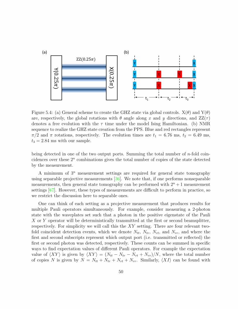
ZZ 0.25
X(Y(
X
X X
XY
Y
Y
X
X
X
t1 t2 t3
(a) (b)
Figure 5.4: (a) General scheme to create the GHZ state via global controls. X(θ) and Y(θ)are, respectively, the global rotations with θ angle along x and y directions, and ZZ(τ)denotes a free evolution with the τ time under the model Ising Hamiltonian. (b) NMRsequence to realize the GHZ state creation from the PPS. Blue and red rectangles representπ/2 and π rotations, respectively. The evolution times are t1 = 6.76 ms, t2 = 6.49 ms,t3 = 2.84 ms with our sample.
being detected in one of the two output ports. Summing the total number of n-fold coin-cidences over these 2n combinations gives the total number of copies of the state detectedby the measurement.
A minimum of 3n measurement settings are required for general state tomographyusing separable projective measurements [36]. We note that, if one performs nonseparablemeasurements, then general state tomography can be performed with 2n + 1 measurementsettings [67]. However, these types of measurements are difficult to perform in practice, sowe restrict the discussion here to separable ones.
One can think of each setting as a projective measurement that produces results formultiple Pauli operators simultaneously. For example, consider measuring a 2-photonstate with the waveplates set such that a photon in the positive eigenstate of the PauliX or Y operator will be deterministically transmitted at the first or second beamsplitter,respectively. For simplicity we will call this the XY setting. There are four relevant two-fold coincident detection events, which we denote Ntt, Ntr, Nrt, and Nrr, and where thefirst and second subscripts represent which output port (i.e. transmitted or reflected) thefirst or second photon was detected, respectively. These counts can be summed in specificways to find expectation values of different Pauli operators. For example the expectationvalue of 〈XY 〉 is given by 〈XY 〉 = (Ntt − Ntr − Nrt + Nrr)/N , where the total numberof copies N is given by N = Ntt + Ntr + Nrt + Nrr. Similarly, 〈XI〉 can be found with
50

Figure 5.5: The reconstruction of density matrix for GHZ state. The upper two figuresare real and imaginary part of density matrix of state reconstruction using all 64 Paulimeasurements. The bottom two figures are real and imaginary part of density matrix ofstate reconstruction using 31 optimum Pauli measurements described in Eq. (5.7). Thefidelity between the two density matrices is 0.960.
〈XI〉 = (Ntt + Ntr −Nrt −Nrr)/N . In total, the XY setting measures the following fourPauli operators:
XY,XI, IY, II.
Based on this observation, we can use the results of Theorem 3 and Theorem 4 toreduce the number of settings to UDA pure states. For the two-qubit case, recall that the
51

0.0
0.2
0.4
0.6
0.8
1.0
Fidelity
Figure 5.6: Performance of 3-qubit protocol using selected Pauli measurements againstrandomly Pauli measurements. Blue dots represents fidelity between density matrix recon-structed from all 64 Pauli measurements and density matrix reconstructed from random 31Pauli measurements. The red squre represents fidelity of reconstruction using our protocol.
11 Pauli operators to UDA any pure states are
A = II, IX, IY, IZ,XI, Y X, Y Y, Y Z, ZX,ZY, ZZ.
Notice that any of the 6 Paulis with no I component (the two-qubit correlations) onlyappear in the setting which measures it. However, looking at the remaining 5 Paulis, IIis included in every setting, IX is included in the Y X setting, IY in Y Y , IZ in Y Z. Theonly operator which does not appear in the settings of the two-qubit correlations is XI, sofor the two qubit case, 6 + 1 = 7 settings are required to be sufficient for UDA.
And similar analysis can be done for the three qubit case, with the aid of computersearch. That is, we find the minimum number of settings that can produce all the 31 Paulioperators as given in Eq. (5.7). We summarize these results as the corollary below.
52

Figure 5.7: Measurement scheme for a polarization-encoded n-photon state. The n-qubitstate is encoded in the polarizations of the n photons. Each photon is measured usinga quarter-waveplate (QWP), half-waveplate (HWP) and a polarizing beamplitter (PBS)with a single-photon counting detector (SPD) at each of its output ports. The quarter- andhalf-waveplates are rotated to choose the measurement basis for each photon. Separableprojective measurements are performed by counting coincident detection events betweenall n photons.
53

Corollary 1. Only 7 settings
XI, Y X, Y Y, Y Z, ZX,ZY, ZZ.
are needed to UDA any two-qubit pure states, compared with 9 settings needed for generaltwo-qubit state tomography. And only 19 settings
XXZ,XY Z,XZX,XZY,XZZ, Y XX,Y XY, Y Y X, Y Y Y, Y ZX, Y ZY, Y ZZ,
ZXX,ZXY,ZXZ,ZY X,ZY Y, ZY Z, ZZX (5.13)
are needed to UDA any three-qubit pure states, compared with 27 settings needed for generalthree-qubit state tomography.
We remark that Corollary 1 is a direct application of Theorem 3 and Theorem 4. Itis possible for even better results to be obtained by including knowledge of settings in thefirst optimization. However, proving sufficiency becomes more difficult in these cases.
54

Chapter 6
Conclusion
In this thesis, we looked at two separate proposal testing quantum mechanics utilizing toolswe found in quantum information. In those proposal, different aspect of quantum mechan-ics are challenged. In the large scale, where the curvature of spacetime is not negligible, atest was proposed to probe the potential important physics that arises at the intersectionof quantum theory and general relativity. The experiment with artificial satellites in Earthorbit proposed in the thesis should be able to refute or be consistent with the alternativequantum optics theory proposed. Many other tests of quantum foundation could be per-formed using similar setup. Going forward, we could observe and capture natural occurringevents and push the experiment to larger scale with more precise detectors
In the small scale, we indirectly tested a cornerstone of quantum mechanics, the Bornrule, by directly testing a quantum symmetry called envariance. For the later proposal, weput a bound for the Born rule for a generalized quantum mechanics theory. Our experimentdemonstrated the quantum symmetry envariance and was able to bound the Born rule. Italso gives us new perspective on Born rule. Future experiment includes testing envariancein a larger system, where the boundary of system and environment could be changed.
In chapter 5, the main question at hand is whether the priori information of statebeing pure helps us reconstruct the quantum state. The usefulness of such information wasproven theoretically for ideal situations, then tested in experiment with noise. We concludesthat the knowledge of quantum state being close to a pure state helps us reconstruct thequantum state. With Pauli observables, 2 and 3 qubits pure state could be reconstructedwith a minimum of 11 and 31 measurements respectively. The next step would be lookingat a larger number of qubits, and what are the optimum sets of observables for statetomography. The result motivates us to look into the structure of quantum states, and
55

make efficient tomography of a multi-qubit system realizable.
56

References
[1] Wonmin Son. Consistent theory for causal non-locality beyond the borns rule. Journalof the Korean Physical Society, 64(4):499–503, 2014.
[2] David Rideout, Thomas Jennewein, Giovanni Amelino-Camelia, Tommaso F Demarie,Brendon L Higgins, Achim Kempf, Adrian Kent, Raymond Laflamme, Xian Ma,Robert B Mann, et al. Fundamental quantum optics experiments conceivable withsatellitesreaching relativistic distances and velocities. Classical and Quantum Gravity,29(22):224011, 2012.
[3] L Vermeyden, X Ma, J Lavoie, M Bonsma, Urbasi Sinha, R Laflamme, andKJ Resch. Experimental test of environment-assisted invariance. Physical ReviewA, 91(1):012120, 2015.
[4] Xian Ma, Tyler Jackson, Hui Zhou, Jianxin Chen, Dawei Lu, Michael D Mazurek,Kent AG Fisher, Xinhua Peng, David Kribs, Kevin J Resch, et al. Pure-state tomog-raphy with the expectation value of pauli operators. Physical Review A, 93(3):032140,2016.
[5] Piotr Kolenderski, Wojciech Wasilewski, and Konrad Banaszek. Modeling and opti-mization of photon pair sources based on spontaneous parametric down-conversion.Physical Review A, 80(1):013811, 2009.
[6] CK Hong and L Mandel. Theory of parametric frequency down conversion of light.Physical Review A, 31(4):2409, 1985.
[7] Harald Weinfurter and Marek Zukowski. Four-photon entanglement from down-conversion. Physical Review A, 64(1):010102, 2001.
[8] James D Franson. Bell inequality for position and time. Physical Review Letters,62(19):2205, 1989.
57

[9] Paul G Kwiat, Aephraim M Steinberg, and Raymond Y Chiao. High-visibility in-terference in a bell-inequality experiment for energy and time. Physical Review A,47(4):R2472, 1993.
[10] Peter van Loock and Akira Furusawa. Detecting genuine multipartite continuous-variable entanglement. Physical Review A, 67(5):052315, 2003.
[11] Keiichi Edamatsu. Entangled photons: generation, observation, and characterization.Japanese Journal of Applied Physics, 46(11R):7175, 2007.
[12] Emanuel Knill, Raymond Laflamme, and Gerald J Milburn. A scheme for efficientquantum computation with linear optics. nature, 409(6816):46–52, 2001.
[13] Rupert Ursin, F Tiefenbacher, T Schmitt-Manderbach, H Weier, Thomas Scheidl,M Lindenthal, B Blauensteiner, T Jennewein, J Perdigues, P Trojek, et al.Entanglement-based quantum communication over 144 km. Nature physics, 3(7):481–486, 2007.
[14] Nicholas David Birrell and Paul Charles William Davies. Quantum fields in curvedspace. Number 7. Cambridge university press, 1984.
[15] TC Ralph. Time displaced entanglement and non-linear quantum evolution. arXivpreprint quant-ph/0510038, 2005.
[16] TC Ralph. A model for nonlinear quantum evolution based on time displaced entan-glement. In SPIE Optics+ Photonics, pages 63050P–63050P. International Society forOptics and Photonics, 2006.
[17] TC Ralph. Unitary solution to a quantum gravity information paradox. PhysicalReview A, 76(1):012336, 2007.
[18] TC Ralph, GJ Milburn, and T Downes. Gravitationally induced decoherence of opticalentanglement. arXiv preprint quant-ph/0609139, 2006.
[19] Timothy C Ralph, Gerard J Milburn, and T Downes. Quantum connectivity of space-time and gravitationally induced decorrelation of entanglement. Physical Review A,79(2):022121, 2009.
[20] David Deutsch. Quantum mechanics near closed timelike lines. Physical Review D,44(10):3197, 1991.
58

[21] Wojciech Hubert Zurek. Probabilities from entanglement, borns rule p k= ψ k 2 fromenvariance. Physical Review A, 71(5):052105, 2005.
[22] Wojciech Hubert Zurek. Environment-assisted invariance, entanglement, and proba-bilities in quantum physics. Physical review letters, 90(12):120404, 2003.
[23] Wojciech Hubert Zurek. Decoherence, einselection, and the quantum origins of theclassical. Reviews of Modern Physics, 75(3):715, 2003.
[24] Wojciech H Zurek. From quantum to classical. PHYSICS TODAY, page 37, 1991.
[25] Maximilian Schlosshauer and Arthur Fine. On zureks derivation of the born rule.Foundations of Physics, 35(2):197–213, 2005.
[26] L Landau. Das dampfungsproblem in der wellenmechanik. Zeitschrift fur Physik,45(5-6):430–441, 1927.
[27] Michael A Nielsen and Isaac L Chuang. Quantum computation and quantum infor-mation. Cambridge university press, 2010.
[28] Max Born. Quantenmechanik der stoßvorgange. Zeitschrift fur Physik, 38(11-12):803–827, 1926.
[29] Taehyun Kim, Marco Fiorentino, and Franco NC Wong. Phase-stable source ofpolarization-entangled photons using a polarization sagnac interferometer. PhysicalReview A, 73(1):012316, 2006.
[30] Alessandro Fedrizzi, Thomas Herbst, Andreas Poppe, Thomas Jennewein, and An-ton Zeilinger. A wavelength-tunable fiber-coupled source of narrowband entangledphotons. Optics Express, 15(23):15377–15386, 2007.
[31] Devon N Biggerstaff, R Kaltenbaek, DR Hamel, G Weihs, T Rudolph, and Kevin JResch. Cluster-state quantum computing enhanced by high-fidelity generalized mea-surements. Physical review letters, 103(24):240504, 2009.
[32] Miroslav Jezek, Jaromır Fiurasek, and Zdenek Hradil. Quantum inference of statesand processes. Physical Review A, 68(1):012305, 2003.
[33] Richard Jozsa. Fidelity for mixed quantum states. Journal of modern optics,41(12):2315–2323, 1994.
59

[34] Anil Bhattacharyya. On a measure of divergence between two multinomial popula-tions. Sankhya: The Indian Journal of Statistics, pages 401–406, 1946.
[35] Daniel F. V. James, Paul G. Kwiat, William J. Munro, and Andrew G. White. Mea-surement of qubits. Phys. Rev. A, 64:052312, Oct 2001.
[36] Mark D. de Burgh, Nathan K. Langford, Andrew C. Doherty, and Alexei Gilchrist.Choice of measurement sets in qubit tomography. Phys. Rev. A, 78:052122, Nov 2008.
[37] Lieven MK Vandersypen and Isaac L Chuang. Nmr techniques for quantum controland computation. Rev. Mod. Phys., 76(4):1037, 2005.
[38] Ivan Oliveira, Roberto Sarthour Jr, Tito Bonagamba, Eduardo Azevedo, and Jair CCFreitas. NMR quantum information processing. Elsevier, 2011.
[39] M. Nielsen and I. Chuang. Quantum Computation and Quantum Information. Cam-bridge University Press, Cambridge, England, 2000.
[40] Jianxin Chen, Hillary Dawkins, Zhengfeng Ji, Nathaniel Johnston, David Kribs, Fred-eric Shultz, and Bei Zeng. Uniqueness of quantum states compatible with given mea-surement results. Physical Review A, 88(1):012109, 2013.
[41] Teiko Heinosaari, Luca Mazzarella, and Michael M Wolf. Quantum tomography underprior information. Communications in Mathematical Physics, 318(2):355–374, 2013.
[42] S. Weigert. Pauli problem for a spin of arbitrary length: A simple method to determineits wave function. Phys. Rev. A, 45:7688–7696, June 1992.
[43] J.-P. Amiet and S. Weigert. Reconstructing a pure state of a spin s through threeStern-Gerlach measurements. J. Phys. A: Math. Gen., 32:2777–2784, April 1999.
[44] J. Finkelstein. Pure-state informationally complete and “really” complete measure-ments. Phys. Rev. A, 70(5):052107, November 2004.
[45] S. T. Flammia, A. Silberfarb, and C. M. Caves. Minimal Informationally CompleteMeasurements for Pure States. Foundations of Physics, 35:1985–2006, December 2005.
[46] Nan Li, Christopher Ferrie, and Carlton M Caves. Fisher-symmetric informationallycomplete measurements for pure states. arXiv preprint arXiv:1507.06904, 2015.
[47] Charles H Baldwin, Ivan H Deutsch, and Amir Kalev. Informational completeness inbounded-rank quantum-state tomography. arXiv preprint arXiv:1510.02736, 2015.
60

[48] Amir Kalev and Charles H Baldwin. The power of being positive: Robust stateestimation made possible by quantum mechanics. arXiv preprint arXiv:1511.01433,2015.
[49] Carmeli, Claudio, Heinosaari, Teiko, Schultz, Jussi, and Toigo, Alessandro. How manyorthonormal bases are needed to distinguish all pure quantum states? Eur. Phys. J.D, 69(7):179, 2015.
[50] D. Gross, Y.-K. Liu, S. T. Flammia, S. Becker, and J. Eisert. Quantum State Tomog-raphy via Compressed Sensing. Phys. Rev. Lett., 105(15):150401, October 2010.
[51] M. Cramer, M. B. Plenio, S. T. Flammia, R. Somma, D. Gross, S. D. Bartlett,O. Landon-Cardinal, D. Poulin, and Y.-K. Liu. Efficient quantum state tomogra-phy. Nat. Commun., 1, December 2010.
[52] Amir Kalev, Robert L Kosut, and Ivan H Deutsch. Quantum tomography protocolswith positivity are compressed sensing protocols. npj Quantum Information, 1:15018,2015.
[53] W.-T. Liu, T. Zhang, J.-Y. Liu, P.-X. Chen, and J.-M. Yuan. Experimental QuantumState Tomography via Compressed Sampling. Phys. Rev. Lett., 108(17):170403, April2012.
[54] Jianxin Chen, Zhengfeng Ji, Bei Zeng, and D. L. Zhou. From ground states to localhamiltonians. Phys. Rev. A, 86:022339, Aug 2012.
[55] J. Chen, Z. Ji, M. B. Ruskai, B. Zeng, and D.-L. Zhou. Comment on some results ofErdahl and the convex structure of reduced density matrices. Journal of MathematicalPhysics, 53(7):072203, July 2012.
[56] Tyler Jackson. Quantum Tomography with Pauli Operators. Master’s thesis, Univer-sity of Guelph, Canada, 2013.
[57] Bei Zeng, Hyeyoun Chung, Andrew W Cross, and Isaac L Chuang. Local unitaryversus local clifford equivalence of stabilizer and graph states. Physical Review A,75(3):032325, 2007.
[58] David G Cory, Amr F Fahmy, and Timothy F Havel. Ensemble quantum computingby nmr spectroscopy. Proc. Natl. Acad. Sci. USA, 94(5):1634–1639, 1997.
61

[59] Dawei Lu, Aharon Brodutch, Jihyun Park, Hemant Katiyar, Tomas Jochym-O’Connor, and Raymond Laflamme. Nmr quantum information processing. arXivpreprint arXiv:1501.01353, 2015.
[60] Yanxiang Gao, Hui Zhou, Dong Zou, Xinhua Peng, and Jiangfeng Du. Preparation ofgreenberger-horne-zeilinger and w states on a one-dimensional ising chain by globalcontrol. Phys. Rev. A, 87:032335, Mar 2013.
[61] J. B. Altepeter, E. R. Jeffrey, and P. G. Kwiat. Phase-compensated ultra-bright sourceof entangled photons. Opt. Express, 13(22):8951–8959, Oct 2005.
[62] Robert Prevedel, Philip Walther, Felix Tiefenbacher, Pascal Bohi, Rainer Kaltenbaek,Thomas Jennewein, and Anton Zeilinger. High-speed linear optics quantum computingusing active feed-forward. Nature, 445(7123):65–69, Jan 2007.
[63] Kai Chen, Che-Ming Li, Qiang Zhang, Yu-Ao Chen, Alexander Goebel, Shuai Chen,Alois Mair, and Jian-Wei Pan. Experimental realization of one-way quantum com-puting with two-photon four-qubit cluster states. Phys. Rev. Lett., 99:120503, Sep2007.
[64] Robert Prevedel, Deny R. Hamel, Roger Colbeck, Kent Fisher, and Kevin J. Resch.Experimental investigation of the uncertainty principle in the presence of quantummemory and its application to witnessing entanglement. Nat. Phys., 7(10):757–761,Oct 2011.
[65] C. Erven, E. Meyer-Scott, K. Fisher, J. Lavoie, B L. Higgins, Z. Yan, C. J. Pugh, J.-P.Bourgoin, R. Prevedel, L. K. Shalm, L. Richards, N. Gigov, R. Laflamme, G. Weihs,T. Jennewein, and K J. Resch. Experimental three-photon quantum nonlocality understrict locality conditions. Nat. Photon., 8(4):292–296, Apr 2014. Letter.
[66] Deny R. Hamel, Lynden K. Shalm, Hannes Hubel, Aaron J. Miller, Francesco Marsili,Varun B. Verma, Richard P. Mirin, Sae Woo Nam, Kevin J. Resch, and Thomas Jen-newein. Direct generation of three-photon polarization entanglement. Nat. Photon.,8(10):801–807, Oct 2014. article.
[67] R. B. A. Adamson and A. M. Steinberg. Improving quantum state estimation withmutually unbiased bases. Phys. Rev. Lett., 105:030406, Jul 2010.
[68] Roger A Horn and Charles R Johnson. Matrix analysis. Cambridge university press,2012.
62

APPENDICES
63

Appendix A
Testing of envariance to Born rulecontinued
From Sec 4.2, the derivation of Born rule consists of two parts, which are presented intwo theorems. We have tested the first part of derivation, where maximumly entangledbipartite is measured, namely the theorem 2. Although this part is undeniable the core ofthe derivation, it is not exactly Born rule. Combined with the second part of the derivation,where probability of getting a eigenstate is related to the modular square of its eigenvalue,the derivation is complete. The second part of the derivation is called ”fine graining” ofthe state, where the pointer state is expanded to a superposition of eigenstates.
Let’s begin with looking at what is the minimum number of qubits needed for thistest. The most simplified example it to show that the state |Φ〉 = 1√
3|0〉 |0〉 +
√2√3|1〉 |1〉
satisfies Born rule. one just have to show that the probability of measuring the first qubitin |0〉 is 2
3and the probability of measuring it in |1〉 is 1
3. We call the first qubit system A,
and the second qubit system B. If system B is large enough, say at least an 6 dimensionHilbertspace, we could add an additional qutrit to system B. The state becomes
|Φ0〉 =
(1√3|0〉 |0〉+
√2√3|1〉 |1〉
)|0〉
=1√3|0〉A |00〉B +
√2√3|1〉A |10〉B (A.1)
Find a transformation acting on system B alone which maps |00〉B to |00〉B and |10〉Bto 1√
2(|11〉B + |02〉B). The state after this transformation becomes
64

|Φ′〉 =1√3|0〉A |00〉B +
1√3|1〉A |11〉B +
1√3|1〉A |02〉B
=1√3|0〉A |0〉B1
|0〉B2+
1√3|1〉A |1〉B1
|1〉B2+
1√3|1〉A |0〉B1
|2〉B2(A.2)
We could use the envariance property of |Φ′〉 to show that the probability of getting|0〉A |0〉B1
, |1〉A |1〉B1and |1〉A |0〉B1
from measuring |Φ′〉 in computational basis are thesame.
We denote the probability of getting |0〉A |0〉B1, P|Φ′〉
(|0〉A |0〉B1
), and the probability
of getting |1〉A |1〉B1, P|Φ′〉
(|1〉A |1〉B1
). If we swap the state |0〉A |0〉B1
and |1〉A |1〉B1on
system A and system B1, we get a updated state
|Φ′〉Swap =1√3|0〉A |0〉B1
|1〉B2+
1√3|1〉A |1〉B1
|0〉B2+
1√3|1〉A |0〉B1
|2〉B2
Note that the swap operation could be done by swapping the measurement outcome|1〉A |1〉B1
and |0〉A |0〉B1. Thus, P|Φ′〉
(|1〉A |1〉B1
)= P|Φ′〉Swap
(|0〉A |0〉B1
)and P|Φ′〉
(|0〉A |0〉B1
)=
P|Φ′〉Swap
(|1〉A |1〉B1
). From the envariance property of |Φ′〉 , we know that the swap
|0〉A |0〉B1and |1〉A |1〉B1
on system A and system B1 could be undone by a swap |1〉B2
and |0〉B2on system B2. The operation on system B2 should not affect the probabili-
ties we got in system A and system B1. Thus, P|Φ′〉(|1〉A |1〉B1
)= P|Φ′〉Swap
(|1〉A |1〉B1
)and P|Φ′〉
(|0〉A |0〉B1
)= P|Φ′〉Swap
(|0〉A |0〉B1
). In sum, we should have P|Φ′〉
(|0〉A |0〉B1
)=
P|Φ′〉(|1〉A |1〉B1
).
Similarly, we could derive P|Φ′〉(|1〉A |0〉B1
)= P|Φ′〉
(|1〉A |1〉B1
). Thus, P|Φ′〉
(|0〉A |0〉B1
)=
P|Φ′〉(|1〉A |0〉B1
)= P|Φ′〉
(|1〉A |1〉B1
), the probability of getting |0〉A |0〉B1
, |1〉A |1〉B1and
|1〉A |0〉B1from measuring |Φ′〉 in computational basis are the same.
Assumes Alice have access to the first and the second qubit of |Φ′〉 and Bob have accessto the first qubit only. Alice should be measuring |00〉, |10〉 and |11〉 with same probabilityfrom the argument above.The measurement result from Bob can’t be conflict with the onefrom Alice, so he should be getting |1〉 twice as much as |0〉. Thus, the probability ofmeasuring |1〉 is 2
3while the probability of measuring |0〉 is 1
3for the first qubit.
By running experiments on envariance testing, we would like to put bounds on theBorn rule.
65

In the previous experiment, we tested envariance for the state |Φ+〉 = 1√2
(|00〉+ |11〉).Ideally for state |Φ+〉, any unitary US on the first qubit could be undone by an unitary
UE on the second qubit. Define US =
(1 00 eiθ
), we could get the corresponding recover
unitary UE =
(1 00 e−iθ
). Note that US ⊗ 1 |Φ+〉 = 1√
2
(|00〉+ eiθ |11〉
), which gives a
relative phase eiθ. This could be undone by operation on the second qubit, which shouldnot affect any probability distribution we can get from the first qubit. We could concludethat probability of measuring |0〉 or |1〉 for the first qubit is independent of the phase eiθ.Moreover, using the argument in section 1.2, we could also conclude that the probabilityof getting|0〉 or |1〉 is 1
2. The experimental result indicates that after operation US⊗UE we
could recover |Φ+〉 with high fidelity. We can’t conclude |Φ+〉 is envariant underUS sincewe can’t get fidelity 1. However, we can try to put bounds on Born rule for state like |Φ+〉once we could get bounds on the experimental errors. (on going)
One might want to consider a more general state |ψSE〉 =∑N
k=1 αk |σk〉 |εk〉, where|αi|2 6= 1
N. To provide evidence or put bound on Born rule for this type of states, additional
experiments are required.
The goal is to perform an experiment to transform the state from |Φ0〉 = 1√3|000〉 +
√2√3|111〉 to |Φ′〉 = 1√
3|000〉 + 1√
3|111〉 + 1√
3|102〉 followed by an experiment to test the
envariance property of the state |Φ′〉. Since qubit is more accessible than qutrit in the lab,we could replace the qutrit with two qubits and use |00〉, |11〉 and |10〉 as our three levelsystem.
We could summarize the task as followed:
1)Construct state |Φ0〉 = 1√3|0000〉 +
√2√3|1111〉, and find a transformation without
touching the first qubit to map |Φ0〉 to |Φ′〉 = 1√3|0000〉+ 1√
3|1111〉+ 1√
3|1010〉
2)Test the state |Φ′〉 = 1√3|0000〉 + 1√
3|1111〉 + 1√
3|1010〉 is envariant under swap op-
erations on the first two qubits. For example, the swap between |00〉 and |11〉 on the firstand second qubit could be undone by the same operation on the third and fourth qubit.
Here we propose a experiment with linear optics. We use polarization of photons asour qubits, where |1〉 = |V 〉 and |0〉 = |H〉. Figure A.1 shows a circuit which outputs
|Φ′〉 = 1√3|0000〉+ 1√
3|1111〉+ 1√
3|1010〉 if we in put |Φ〉 = 1√
3|0〉 |0〉+
√2√3|1〉 |1〉 at node A
and B.
To understand what does the circuit in Figure A.1 does, first we take a closer look atwhat the elements in the blue dash line box do A.1. If the detector 1 detects a photon
66

Input state |>
Detector 1
Detector 2
C
A B
D
E F G
H
PBS1
PBS2 PBS3
PBS4
J
Figure A.1: Testing “Fine graining”.The input state at A and B is|Φ〉 = 1√3|0〉 |0〉 +
√2√3|1〉 |1〉. where |0〉 = |H〉 represents horizontal polarization |1〉 = |V 〉 represents vertical
polarization. Node C prepares a pair of photons in the state 1√2|0〉 |0〉 + 1√
2|1〉 |1〉, while
Node D emits a single photon with random polarization. Upon detect exactly one photon atdetector 1 and detector 2, The state coming out from E,F,G,H could be |Φ′〉 = 1√
3|0000〉+
1√3|1100〉+ 1√
3|1111〉
67

Detector 1 CPBS1
A
E
C1
C2
Figure A.2: Preparation of entangled state α|00〉+ β|11〉
in horizontal polarization, that photon must coming from C1. The photon in C2 shouldbe in horizontal polarization as well since we prepared 1√
2|0〉 |0〉 + 1√
2|1〉 |1〉 at node C.
Moreover, the photon from A should be in horizontal polarization since it went throughthe PBS. Thus, the photon in C2 and E are both in |0〉. Similarly, if detector 1 detect aphoton in vertical polarization, the photon in C2 and B are both in |1〉. Upon post selectexactly one photon detected at detector 1, we know that the state in B and C2 shouldhave the form α |0〉 |0〉+ β |1〉 |1〉.
The elements in the red dash line box is a C-NOT gate upon detect one photon atdetector 2. We could conjugate the C-NOT gate with two π
4− Z gate to get a controlled-
Hadamard gate.
Thus, if we input |Φ〉 = 1√3|0〉A |0〉B +
√2√3|1〉A |1〉B, the elements in the blue box will
transform the state into 1√3|0〉E |0〉F |0〉B +
√2√3|1〉E |1〉F |1〉B . The controlled-Hadamard
gate will further transform the state into 1√3|0〉E |0〉F |0〉B+ 1√
3|1〉E |1〉F |0〉B′+ 1√
3|1〉E |1〉F |1〉B′ .
We consider the spatial degree of freedom for the photon through PBS4 as our fourth qubit.Thus, we get the state coming out from E,F,G,H could be |Φ′〉 = 1√
3|0000〉 + 1√
3|1100〉 +
68

1√3|1111〉.
Once we have prepared state |Φ′〉 = 1√3|0000〉+ 1√
3|1010〉+ 1√
3|1111〉, we could proceed
to test the envariance operation for state |Φ′〉. We would like to swap |00〉 and |10〉 for thefirst two qubits, and see if the same swap operation for the last two qubits recovers |Φ′〉.We propose the two possible tests as followed:
1)Perform a state tomography experiment, and get the 16×16 density matrix ρ for theoutput state|Φ′〉. The swap operations could be done by rearrange the rows and columns ofρ . Ideally, after swapping |00〉 and |10〉 for the first two qubits and the last two qubits, weshould get the same ρ . The possible deviation from ρ could come from either experimentalerror or the failure of envariance theory.
2)Pick a random orthonormal basis Bi and measure |Φ′〉 with this basis. After largenumber of trials, we could estimate the probability Pi of getting outcome Bi. Then weswap |00〉 and |10〉 for the first two qubits and same for the last two qubits for all Bi , andwe could get another orthonormal basis B′i . Measure |Φ′〉 with B′i, and estimate theprobability P ′i of getting outcome Bi. We will have two arrays at the end of experiment,Pi and P ′i. Ideally they should be the same. Any difference should come from eitherexperimental error or the failure of envariance theory.
69

Appendix B
Proof of UDA using selected Paulisfor 3 qubits
In order to prove Theorem 4, it suffices to prove the following result.
Theorem 5. Any Hermitian operator perpendicular to
IIX, IIY, IIZ, IXI, IXX, IXY, IY I, IY X, IY Y, IZI,XIZ,XXX,XXY,XY X,XY Y,XZX,XZY, Y XX,
Y XY, Y XZ, Y Y X, Y Y Y, Y Y Z, Y ZI, ZII, ZXZ,ZY Z,
ZZX,ZZY, ZZZ (B.1)
must have at least two positive and two negative eigenvalues.
Proof. The proof proceeds as follows. First construct an 8-by-8 traceless Hermitian ma-trix H which is orthogonal to all the above Pauli operators. This will be a real linearcombination of every Pauli operator that is not being measured. This H is then a generaldescription of any Hermitian matrix in the complement of the span of all measured op-erators. We will show through a case by case analysis that if we assume H only has onepositive eigenvalue, then it follows that H must be the zero matrix. A similar argumentholds for having only one negative eigenvalue therefore H must have at least two positiveand two negative eigenvalues.
Let us begin by constructing H which is a real linear combination of the 33 Paulioperators not being measured (excluding the identity). H is then:
70

H = x1IXZ + x2IY Z + x3IZX + x4IZY
+x5IZZ + x6XII + x7XIX + x8XIY
+x9XXI + x10XXZ + x11XY I + x12XY Z
+x13XZI + x14XZZ + x15Y II + x16Y IX
+x17Y IY + x18Y IZ + x19Y XI + x20Y Y I
+x21Y ZX + x22Y ZY + x23Y ZZ + x24ZIX
+x25ZIY + x26ZIZ + x27ZXI + x28ZXX
+x29ZXY + x30ZY I + x31ZY X + x32ZY Y
+x33ZZI.
Writing H in matrix form will give the form:
c11 c12 c13 c14 c15 c16 c17 0c∗12 c22 c23 c24 c25 c26 0 c28
c∗13 c∗23 c33 c34 c35 0 c37 c38
c∗14 c∗24 c∗34 c44 0 c46 c47 c48
c∗15 c∗25 c∗35 0 c55 c56 c57 c58
c∗16 c∗26 0 c∗46 c∗56 c66 c67 c68
c∗17 0 c∗37 c∗47 c∗57 c∗67 c77 c78
0 c∗28 c∗38 c∗48 c∗58 c∗68 c∗78 c88
(B.2)
71

where
c11 = x5 + x26 + x33;
c22 = −x5 − x26 + x33;
c33 = −x5 + x26 − x33;
c44 = x5 − x26 − x33;
c55 = x5 − x26 − x33 = c44;
c66 = −x5 + x26 − x33 = c33;
c77 = −x5 − x26 + x33 = c22;
c88 = x5 + x26 + x33 = c11;
c12 = x3 + x24 − i(x4 + x25);
c34 = −x3 + x24 + i(x4 − x25);
c56 = x3 − x24 − i(x4 − x25) = −c34;
c78 = −x3 − x24 + i(x4 + x25) = −c12;
c13 = x1 + x27 − i(x2 + x30);
c24 = −x1 + x27 + i(x2 − x30);
c57 = x1 − x27 − i(x2 − x30) = −c24;
c68 = −x1 − x27 + i(x2 + x30) = −c13;
c14 = x28 − x32 − i(x29 + x31);
c23 = x28 + x32 + i(x29 − x31);
c58 = −x28 + x32 + i(x29 + x31) = −c14;
c67 = −x28 − x32 − i(x29 − x31) = −c23;
c15 = x6 + x13 + x14 − i(x15 + x18 + x23);
c26 = x6 + x13 − x14 − i(x15 − x18 − x23);
c37 = x6 − x13 − x14 − i(x15 + x18 − x23);
c48 = x6 − x13 + x14 − i(x15 − x18 + x23)
= c15 − c∗26 + c∗37;
c16 = x7 − x17 − x22 − i(x8 + x16 + x21);
c25 = x7 + x17 + x22 + i(x8 − x16 − x21);
c38 = x7 − x17 + x22 − i(x8 + x16 − x21);
c47 = x7 + x17 − x22 + i(x8 − x16 + x21)
= c∗16 + c25 − c∗38;
72

c17 = x9 + x10 − x20 − i(x11 + x12 + x19);
c28 = x9 − x10 − x20 − i(x11 − x12 + x19);
c35 = x9 + x10 + x20 + i(x11 + x12 − x19);
c46 = x9 − x10 + x20 + i(x11 − x12 − x19)
= c∗28 + c35 − c∗17;
Note that the anti-diagonal terms are all zeros. This was by design, since any set ofPauli operators Clifford equivalent to the result from the hyper-graph dualization programis also a solution, we had the freedom to choose a set which would make the proof simpler.Choosing the set of operators which contained all Pauli operators constructed by tensoringonly X operators and Y operators meant H would have zero main anti-diagonal. The onlyreason for choosing this set is it makes this proof a little simpler.
Here we assume H is a Hermitian matrix with only one positive eigenvalue. We firstshow all diagonal entries of H must be zero. Observe that c55 = c44, c66 = c33, c77 =c22, c88 = c11. In order for the traceless condition on H to hold, it is then clear thatc11 + c22 + c33 + c44 = 0. If H has some nonzero diagonal entry, then at least one ofc11, c22, c33 and c44 will be positive. Without loss of generality, let c11 > 0, then thesubmatrix of H formed by the rows (1, 8) and columns (1, 8), which will be of the formc11 ∗ I, will have two positive eigenvalues.
Lemma 1. Cauchy’s Interlacing Theorem states[68]:Let:
A =
[B CC† D
]be an n-by-n Hermitian matrix, where B has size m-by-m (m<n). If the eigenvalues of Aand B are α1 ≤ . . . ≤ αn and β1 ≤ . . . ≤ βm respectively. Then:
αk ≤ βk ≤ αk+n−m, k = 1, . . . ,m.
It follows from Cauchy’s interlacing property that if a principle submatrix of H has 2positive eigenvalues then H also has at least two positive eigenvalues.
Hence, H must be in the following form:
73
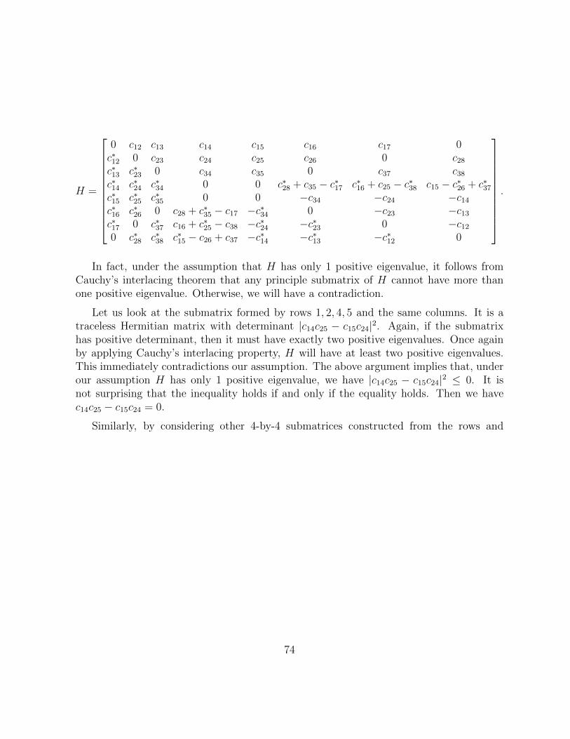
H =
0 c12 c13 c14 c15 c16 c17 0c∗12 0 c23 c24 c25 c26 0 c28
c∗13 c∗23 0 c34 c35 0 c37 c38
c∗14 c∗24 c∗34 0 0 c∗28 + c35 − c∗17 c∗16 + c25 − c∗38 c15 − c∗26 + c∗37
c∗15 c∗25 c∗35 0 0 −c34 −c24 −c14
c∗16 c∗26 0 c28 + c∗35 − c17 −c∗34 0 −c23 −c13
c∗17 0 c∗37 c16 + c∗25 − c38 −c∗24 −c∗23 0 −c12
0 c∗28 c∗38 c∗15 − c26 + c37 −c∗14 −c∗13 −c∗12 0
.
In fact, under the assumption that H has only 1 positive eigenvalue, it follows fromCauchy’s interlacing theorem that any principle submatrix of H cannot have more thanone positive eigenvalue. Otherwise, we will have a contradiction.
Let us look at the submatrix formed by rows 1, 2, 4, 5 and the same columns. It is atraceless Hermitian matrix with determinant |c14c25 − c15c24|2. Again, if the submatrixhas positive determinant, then it must have exactly two positive eigenvalues. Once againby applying Cauchy’s interlacing property, H will have at least two positive eigenvalues.This immediately contradictions our assumption. The above argument implies that, underour assumption H has only 1 positive eigenvalue, we have |c14c25 − c15c24|2 ≤ 0. It isnot surprising that the inequality holds if and only if the equality holds. Then we havec14c25 − c15c24 = 0.
Similarly, by considering other 4-by-4 submatrices constructed from the rows and
74

columns a, b, 4, 5 where a, b are any two of the remain six rows, we can show that:
c14c35 − c15c34 = 0;
−c14c∗34 − c15(c28 + c∗35 − c17) = 0;
−c14c∗24 − c15(c16 + c∗25 − c38) = 0;
−c14c∗14 − c15(c∗15 − c26 + c37) = 0;
c24c35 − c25c34 = 0;
−c24c∗34 − c25(c28 + c∗35 − c17) = 0;
−c24c∗24 − c25(c16 + c∗25 − c38) = 0;
−c24c∗14 − c25(c∗15 − c26 + c37) = 0;
−c34c∗34 − c35(c28 + c∗35 − c17) = 0;
−c34c∗24 − c35(c16 + c∗25 − c38) = 0;
−c34c∗14 − c35(c∗15 − c26 + c37) = 0;
−c∗24(c28 + c∗35 − c17) + c∗34(c16 + c∗25 − c38) = 0;
−c∗14(c28 + c∗35 − c17) + c∗34(c∗15 − c26 + c37) = 0;
−c∗14(c16 + c∗25 − c38) + c∗24(c∗15 − c26 + c37) = 0.
The above equations will imply that the 8-by-2 submatrix formed by the 4-th and 5-thcolumns has rank at most 1.
The same argument can be used to prove that the 8-by-2 submatrices formed by columns(1, 8), (2, 7) or (3, 6) also have rank at most 1.
As a straightforward consequence, H has rank no more than 4.
In other words, the k-th column and the (9−k)-th column are linearly dependent. Thismeans that there exist λ1, λ2, λ3, λ4 such that the following equations hold:
λ1−→C1 + (1− λ1)
−→C8 = λ2
−→C2 + (1− λ2)
−→C7 = 0 (B.3)
λ3
−→C3 + (1− λ3)
−→C6 = λ4
−→C4 + (1− λ4)
−→C5 = 0 (B.4)
Here we have used−→Ck to represent the k-th column of the matrix (B.3).
Let us start with a special case. Let λ1 = 0. Then c12 = c13 = c14 = c28 = c38 = 0 andc15 = c∗26 − c∗37. H can be simplified as the following:
75

H =
0 0 0 0 c∗26 − c∗37 c16 c17 00 0 c23 c24 c25 c26 0 00 c∗23 0 c34 c35 0 c37 00 c∗24 c∗34 0 0 c35 − c∗17 c∗16 + c25 0
c26 − c37 c∗25 c∗35 0 0 −c34 −c24 0c∗16 c∗26 0 c∗35 − c17 −c∗34 0 −c23 0c∗17 0 c∗37 c16 + c∗25 −c∗24 −c∗23 0 00 0 0 0 0 0 0 0
.
If we set c23 = c24 = c34 = 0, then the top-left 4-by-4 submatrix is zero. In this case, thecharacteristic polynomial of H contains only even powers. Thus H has only one positiveeigenvalue implies H has only one negative eigenvalue too. As a consequence, the top-right4-by-4 submatrix of H has rank exactly 1.
As a result, any 2-by-2 submatrix of the top-right submatrix must have determinantzero. From suitable choices of submatrices we can obtain the following equations:
c26c37 = 0; (B.5)
c26(c∗26 − c∗37) = c16c25; (B.6)
c37(c∗26 − c∗37) = c17c35; (B.7)
c16(c∗16 + c25) + c17(c∗17 − c35) = 0. (B.8)
Using the above equations we can obtain:
0 = c16(c∗16 + c25) + c17(c∗17 − c35)
= c16c25 − c17c35 + |c17|2 + |c16|2
= c26(c∗26 − c∗37)− c37(c∗26 − c∗37) + |c17|2 + |c16|2
= |c26 − c37|2 + |c17|2 + |c16|2 (B.9)
This implies c16 = c17 = 0 and c26 = c37. Also since c26c37 = 0 we know that c26 = c37 = 0.Furthermore c25(c∗16+c25) = 0 and c35(c35−c∗17) = 0 will guarantee c25 = c35 = 0. ThereforeH is once again the zero matrix.
We must then assume at least one of c23, c24, c34 must be nonzero. If c23 6= 0, thenby considering submatrices formed by rows/columns (1, 2, 3, k) (5 ≤ k ≤ 8), we have
76

c16 = c17 = 0 and c26 = c37. For the case that c24 = 0 or c34 = 0, we will also havec16 = c17 = 0 and c26 = c37 by considering appropriately chosen submatrices.
We are then left with H in the form:
H =
0 0 0 0 0 0 0 00 0 c23 c24 c25 c26 0 00 c∗23 0 c34 c35 0 c26 00 c∗24 c∗34 0 0 c35 c25 00 c∗25 c∗35 0 0 −c34 −c24 00 c∗26 0 c∗35 −c∗34 0 −c23 00 0 c∗26 c∗25 −c∗24 −c∗23 0 00 0 0 0 0 0 0 0
.
Now, recall the fact that the submatrices formed by the k-th and the (9−k)-th columnswill always have rank 1. From this it can be shown we will have H is a zero matrix.
Take the submatrix formed by the second and seventh columns for example. Since theyare linearly dependent, the determinant of any 2-by-2 submatrix must be zero. From thiswe can get that |c23|2 + |c26|2 = 0. Therefore c23 = c26 = 0. By similar arguments onvarious submatrices, H can be shown to be the zero matrix.
Thus, under our assumption that H has exactly one positive eigenvalue, λ1 6= 0. Sim-ilarly, we can also prove that λ1 6= 1, λ2, λ3, λ4 6= 0, 1. We can then assume from now onthat H has no zero columns or rows.
Hence, there exists certain λ1, λ2, λ3 and λ4 6= 0, 1 which satisfies equation B.3.
Let us use < and = to denote the real part and imaginary part of a complex number.Then the above equations can be rewritten as linear equations of real numbers.
Let us use M(λ1, λ2, λ3, λ4) to denote the 48-by-30 coefficient matrix. If we can provethat the coefficient matrix always has rank 30 for any λ1, λ2, λ3 and λ4, then it will implythat all cij’s are zeros which will immediately contradict our assumption.
Unfortunately, we are not that lucky. M(λ1, λ2, λ3, λ4) will be degenerate under certainassignment of variables (λ1, λ2, λ3, λ4). For example, rank(M(1+i
2, 1+i
2, 1+i
2, 1+i
2)) = 27 <
30. However, we can still show that M(λ1, λ2, λ3, λ4) will have rank 30 except for some
77

degenerate cases which will be dealt with separately . The top-left 2-by-2 submatrix hasrank 2 if and only if λ1 6= 0
At least one of the following situations must happen:
1.
[−C1 A1
B2 C2
]has full rank. This implies c12 = c17 = 0.
2.
[A1 C1
−D2 A2
]has full rank. This implies c12 = c28 = 0.
3.
[B3 C3
−C1 A1
]has full rank. This implies c13 = c16 = 0.
4.
[A1 C1
−D3 A3
]has full rank. This implies c13 = c38 = 0.
5.
[−C1 A1
B4 C4
]has full rank. This implies c14 = c15 = 0.
6.
[−C2 A2
B3 C3
]has full rank. This implies c23 = c26 = 0.
7.
[A2 C2
−D3 A3
]has full rank. This implies c23 = c37 = 0.
8.
[−C2 A2
B4 C4
]has full rank. This implies c24 = c25 = 0.
9.
[−C3 A3
B4 C4
]has full rank. This implies c34 = c35 = 0.
78

10.
det
([−C1 A1
B2 C2
])= det
([A1 C1
−D2 A2
])= det
([B3 C3
−C1 A1
])= det
([A1 C1
−D3 A3
])= det
([−C1 A1
B4 C4
])= det
([−C2 A2
B3 C3
])= det
([A2 C2
−D3 A3
])= det
([−C2 A2
B4 C4
])= det
([−C3 A3
B4 C4
])= 0.
With assistance of symbolic computation package like Mathematica, we find that theonly solution to the above equations is <λ1 = <λ2 = <λ3 = <λ4 = 1
2.
Here we will prove that there is no Hermitian matrix in the form ( B.3) with only onepositive eigenvalue for every situations:
1. c12 = c17 = 0. Any H with only one positive eigenvalue must be in the followingform:
H =
0 0 c13 c14 c15 c16 0 00 0 c23 c24 c25 c26 0 c28
c∗13 c∗23 0 c34 c35 0 c37 c38
c∗14 c∗24 c∗34 0 0 c∗28 + c35 c∗16 + c25 − c∗38 c15 − c∗26 + c∗37
c∗15 c∗25 c∗35 0 0 −c34 −c24 −c14
c∗16 c∗26 0 c28 + c∗35 −c∗34 0 −c23 −c13
0 0 c∗37 c16 + c∗25 − c38 −c∗24 −c∗23 0 00 c∗28 c∗38 c∗15 − c26 + c37 −c∗14 −c∗13 0 0
.
By considering submatrices formed by row/columns (1, 2, p, q) where 3 ≤ p < q ≤ 8,we have that the first two rows are linearly dependent. Under our assumption thatthere is no row of H containing only zero entries, we have c28 = 0.
Recall that the 4-th and 5-th rows are linearly dependent, thus c34(−c∗34) = c35(c28 +c∗35) which now can be simplified as |c34|2 + |c35|2 = 0. Hence c34 = c35 = 0. Then
79

H =
0 0 c13 c14 c15 c16 0 00 0 c23 c24 c25 c26 0 0c∗13 c∗23 0 0 0 0 c37 c38
c∗14 c∗24 0 0 0 0 c∗16 + c25 − c∗38 c15 − c∗26 + c∗37
c∗15 c∗25 0 0 0 0 −c24 −c14
c∗16 c∗26 0 0 0 0 −c23 −c13
0 0 c∗37 c16 + c∗25 − c38 −c∗24 −c∗23 0 00 0 c∗38 c∗15 − c26 + c37 −c∗14 −c∗13 0 0
.
Again, by applying our submatrix argument, we have the submatrix formed by(3, 4, 5, 6) columns must has rank 1.
If there is a zero element in the submatrix formed by rows (1, 2, 7, 8) and columns(3, 4, 5, 6), then there must be a row or a column containing only zero elements in H.So, here we assume the submatrix formed by rows (1, 2, 7, 8) and columns (3, 4, 5, 6)does not contain any zero element.
Then c15c25
= c13c23
= c38c37
which implies c38c25 = c37c15.
Follows from the rank 1 condition, we have
c15(c∗15 − c26 + c37) = −|c14|2,c25(c16 + c∗25 − c38) = −|c24|2.
By substituting c38c25 = c37c15 and c15c26 = c25c16 into the above two equations, wehave
|c15|2 + |c14|2 = c15c26 − c15c37
= c25c16 − c25c38
= −|c24|2 − |c25|2
which implies c15 = c14 = c24 = c25 = 0. However, it contradicts our assumption thatthere is no zero element in the submatrix formed by (1, 2, 7, 8) rows and (3, 4, 5, 6)columns.
Similarly, we can also prove that there is no Hermitian matrix in the form B.3 withonly one positive eigenvalue if any of the following conditions apply.
2. c12 = c28 = 0.
80

3. c13 = c16 = 0.
4. c13 = c38 = 0.
5. c14 = c15 = 0.
6. c23 = c26 = 0.
7. c23 = c37 = 0.
8. c24 = c25 = 0.
9. c34 = c35 = 0.
Now, the only case we left is the following:
10. <λ1 = <λ2 = <λ3 = <λ4 = 12. In this case, rank(
[−C1 A1
B2 C2
]) = 3. Hence
(<c12,=c12,<c17,=c17) lies in the nullspace of
[−C1 A1
B2 C2
]=
−1
2−b1
12
b1
b1 −12
b1 −12
12−b2
12
b2
b212−b2
12
.
Thus
[c12 : c17]
= [2(b2 − b1) + (1 + 4b1b2)i : 2(b1 + b2) + (4b1b2 − 1)i].
81

Similarly, we will have
[c12 : c17 : c28]
= [2(b2 − b1) + (1 + 4b1b2)i :
2(b1 + b2) + (4b1b2 − 1)i : −2(b1 + b2)− (4b1b2 − 1)i];
[c13 : c16 : c38]
= [2(b1 − b3)− (1 + 4b1b3)i :
−2(b1 + b3)− (4b1b3 − 1)i : 2(b1 + b3) + (4b1b3 − 1)i];
[c23 : c26 : c37]
= [2(b3 − b2) + (4b2b3 + 1)i :
2(b2 + b3) + (4b2b3 − 1)i : −2(b2 + b3)− (4b2b3 − 1)i];
[c14 : c15]
= [2(b4 − b1)− (4b1b4 + 1)i :
2(b1 + b4) + (4b1b4 − 1)i];
[c24 : c25]
= [2(b4 − b2) + (4b2b4 + 1)i :
2(b2 + b4) + (4b2b4 − 1)i];
[c34 : c35]
= [2(b4 − b3) + (4b3b4 + 1)i :
2(b3 + b4) + (4b3b4 − 1)i].
Here [ q1 : q2 : · · · : qm] = [r1 + s1i : r2 + s2i : · · · : rm + smi] means there exists someµ ∈ R such that qi = µ(ri + sii) for any 1 ≤ i ≤ m.
Observe that c28 = −c17, c38 = −c16, c37 = −c26, we thus simplify the matrix form ofH as the following:
H =
0 c12 c13 c14 c15 c16 c17 0c∗12 0 c23 c24 c25 c26 0 −c17
c∗13 c∗23 0 c34 c35 0 −c26 −c16
c∗14 c∗24 c∗34 0 0 c35 − 2c∗17 c25 + 2c∗16 c15 − 2c∗26
c∗15 c∗25 c∗35 0 0 −c34 −c24 −c14
c∗16 c∗26 0 c∗35 − 2c17 −c∗34 0 −c23 −c13
c∗17 0 −c∗26 c∗25 + 2c16 −c∗24 −c∗23 0 −c12
0 −c∗17 −c∗16 c∗15 − 2c26 −c∗14 −c∗13 −c∗12 0
.
82

It follows from the fact that the submatrix formed by 4-th and 5-th columns hasrank exactly 1, we have c14(−c∗14) = c15(c∗15−2c26). Thus at least one of the followingcases must happen:
(10.1) c14 = c15 = 0. We can still assume there is no column containing only zeroelements as this is the case that we have already discussed. Thus c26 = 0 whichwould also lead to c23 = 0.
(10.2) c26 = c∗15.
Similarly, at least one of the following conditions:
(10.I) c24 = c25 = c16 = c13 = 0; or
(10.II) c16 = −c∗25
and one of the following conditions:
(10.A) c34 = c35 = c17 = c12 = 0; or
(10.B) c17 = c∗35
must apply.
We have already discussed the cases that c12 = c17 = 0, c13 = c16 = 0 or c23 = c26 = 0previously. Hence the only remaining case is c26 = c∗15, c16 = −c∗25, c17 = c∗35. Thus
H =
0 c12 c13 c14 c15 −c∗25 c∗35 0c∗12 0 c23 c24 c25 c∗15 0 −c∗35
c∗13 c∗23 0 c34 c35 0 −c∗15 c∗25
c∗14 c∗24 c∗34 0 0 −c35 −c25 −c15
c∗15 c∗25 c∗35 0 0 −c34 −c24 −c14
−c25 c15 0 −c∗35 −c∗34 0 −c23 −c13
c35 0 −c15 −c∗25 −c∗24 −c∗23 0 −c12
0 −c35 c25 −c∗15 −c∗14 −c∗13 −c∗12 0
.
According to c26 = c∗15, we have 2(b2 + b3)(1− 4b1b4) = (4b2b3 − 1)(2b1 + 2b4) whichimplies 4(b1b2b3 + b1b2b4 + b1b3b4 + b2b3b4) = b1 + b2 + b3 + b4.
1. 4b1b2 + 4b1b3 + 4b2b3 = 1. Thus b1 + b2 + b3 = 4b1b2b3. However, one can easy toverify that there do not exist three real numbers b1, b2, b3 satisfying these twoequations.
83

2. 4b1b2 + 4b1b3 + 4b2b3 6= 1. Hence b4 = b1+b2+b3−4b1b2b34b1b2+4b1b3+4b2b3−1
. By substituting the
84

assignment of b4 into Equation B.10, we have
c14 = p ·(
2(1− 4b21)(b2 + b3) + 4b1(1− 4b2b3)
4b1b2 + 4b1b3 + 4b2b3 − 1
+−8b1(b2 + b3) + (1− 4b2
1)(1− 4b2b3)
4b1b2 + 4b1b3 + 4b2b3 − 1i
);
c15 = p ·(
2(1 + 4b21)(b2 + b3)
4b1b2 + 4b1b3 + 4b2b3 − 1
+(1 + 4b2
1)(1− 4b2b3)
4b1b2 + 4b1b3 + 4b2b3 − 1i
);
c23 = p ·(
2(1 + 4b21)(b3 − b2)
4b1b2 + 4b1b3 + 4b2b3 − 1
+(1 + 4b2
1)(1 + 4b2b3)
4b1b2 + 4b1b3 + 4b2b3 − 1i
);
c24 = q ·(
2(1− 4b22)(b1 + b3) + 4b2(1− 4b1b3)
4b1b2 + 4b1b3 + 4b2b3 − 1
+8b2(b1 + b3)− (1− 4b2
2)(1− 4b1b3)
4b1b2 + 4b1b3 + 4b2b3 − 1i
);
c25 = q ·(
2(1 + 4b22)(b1 + b3)
4b1b2 + 4b1b3 + 4b2b3 − 1
+(1 + 4b2
2)(1− 4b1b3)
4b1b2 + 4b1b3 + 4b2b3 − 1i
);
c13 = q ·(
2(1 + 4b22)(b1 − b3)
4b1b2 + 4b1b3 + 4b2b3 − 1
− (1 + 4b22)(1 + 4b1b3)
4b1b2 + 4b1b3 + 4b2b3 − 1i
);
c34 = r ·(
2(1− 4b23)(b1 + b2) + 4b3(1− 4b1b2)
4b1b2 + 4b1b3 + 4b2b3 − 1
+8b3(b1 + b2)− (1− 4b2
3)(1− 4b1b2)
4b1b2 + 4b1b3 + 4b2b3 − 1i
);
c35 = r ·(
2(1 + 4b23)(b1 + b2)
4b1b2 + 4b1b3 + 4b2b3 − 1
+(1 + 4b2
3)(1− 4b1b2)
4b1b2 + 4b1b3 + 4b2b3 − 1i
);
c12 = r ·(
2(1 + 4b23)(b2 − b1)
4b1b2 + 4b1b3 + 4b2b3 − 1
+(1 + 4b2
3)(1 + 4b1b2)
4b1b2 + 4b1b3 + 4b2b3 − 1i
).
85

Again, with assistance of symbolic computation package like Mathematica, wecan verify that the characteristic polynomial of H contains only even powers.This implies H has nonzero eigenvalue λ if and only if it also has eigenvalue −λ.Therefore, under our assumption that H has only 1 positive eigenvalue, H alsohas only 1 negative eigenvalue.
However, let us consider the 3-by-3 submatrix of H formed by (5, 7, 8)-th rowsand (1, 2, 3)-th columns . Its determinant is (−i + 2b1)(i + 2b1)2(1 + 2ib2)(i +2b2)2(i−2b3)2(i+2b3)2r((1+4b2
1)p2+(1+4b22)q2+(1+4b2
3)r2). It is always nonzerounless p = q = r or r = 0. If r = 0 this implies that c12 = c34 = c35 = 0. Thiscase has already been covered, Thus H has rank at least 3 which contradictsour previous conclusion that H has only one positive eigenvalue and only onenegative eigenvalue.
To summarize, under our assumption that H has only one positive eigenvalue, a con-tradiction always exist in every situation we studied. Hence, H must has at least 2 positiveeigenvalues and at least 2 negative eigenvalues. This completes our proof.
86