WP/09/79

Exposure to Real Estate Losses: Evidence from the U.S. Banks

Deniz Igan and Marcelo Pinheiro

© 2009 International Monetary Fund WP/09/79 IMF Working Paper Research Department

Exposure to Real Estate Losses: Evidence from the U.S. Banks

Prepared by Deniz Igan and Marcelo Pinheiro†

Authorized for distribution by Stijn Claessens

April 2009

Abstract

This Working Paper should not be reported as representing the views of the IMF. The views expressed in this Working Paper are those of the author(s) and do not necessarily represent those of the IMF or IMF policy. Working Papers describe research in progress by the author(s) and are published to elicit comments and to further debate.

We implement a three-step procedure to assess the extent of exposure to real estate in commercial banks. First, we demonstrate interest rates and income to be the major determinants of delinquency. Then, we adopt a stress testing approach to calculate the impact of any adverse changes in these determinants. This suggests that a 1.3 percentage point increase in mortgage interest rate leads to a 20 percent decrease in a typical bank's distance to default. Finally, we look at the cross-sectional differences and indentify the banks with rapid loan growth along with high cost-income ratio as the most vulnerable.

JEL Classification Numbers: D10, E32, G21, R33. Keywords: Residential and Commercial Real Estate, Delinquency, Distance to Default. Author’s E-Mail Address: digan@imf.org, mpinheiro@cornerstone.com

† The authors thank Steven Ott, Stijn Claessens, and two anonymous referees for their comments on earlier drafts. Marcelo Pinheiro is an associate at Cornerstone Research, Washington, D.C. The material discussed herein may not reflect the opinions of Cornerstone Research.

2

Contents Page

I. Introduction ............................................................................................................................3

II. Related Literature..................................................................................................................4

III. Empirical Approach .............................................................................................................6 A. Modeling the Determinants of Delinquencies ..........................................................8 B. Stress Testing ............................................................................................................9 C. Determinants of Vulnerability.................................................................................10

IV. Data....................................................................................................................................11

V. Results.................................................................................................................................12 A. What Leads to Delinquencies?................................................................................12 B. Can the Banking Sector Survive an Economic Downturn? ....................................13 C. Who are the Vulnerable Banks?..............................................................................13 D. What is the Likely Impact of Recent Regulations?.................................................15

VI. Conclusion .........................................................................................................................15

References................................................................................................................................17 Tables Table 1. Definition and Source of Variables ...........................................................................28 Table 2. Summary Statistics ....................................................................................................29 Table 3. VEC Estimation Results: Delinquency rate on real estate loans ...............................30 Table 4. VEC Estimation Results: Delinquency rate on residential real estate loans..............31 Table 5. VEC Estimation Results: Delinquency rate on commercial real estate loans ...........32 Table 6. Summary Statistics by Vulnerability .........................................................................32 Table 7. Characteristics of Vulnerable Banks: Cross-Section Analysis ..................................33 Table 8. Characteristics of Vulnerable Banks: Panel Data Analysis .......................................33 Table 9. Most Vulnerable Banks: Distribution by State ..........................................................33 Figures Figure 1. Business, Credit, and Real Estate Cycles, 1976-2006..............................................18 Figure 2. Share of All Real Estate-Related Loans in Banks' Portfolio, 1960-2006.................19 Figure 3. Share of Real Estate Loans in Banks' Portfolio, 1996-2006 ....................................20 Figure 4. Real Estate Price Indices, 1984-2006.......................................................................21 Figure 5. Real Estate Exposure: Median Bank, 2000-2006.....................................................22 Figure 6. Delinquency Rate, 1991-2006 ..................................................................................23 Figure 7. Response of Delinquency Rate on Real Estate Loans to Major Determinants ........24 Figure 8. Response of Delinquency Rate on Residential Real Estate Loans to Major Determinants ............................................................................................................................25 Figure 9. Response of Delinquency Rate on Commercial Real Estate Loans to Major Determinants ............................................................................................................................26 Figure 10. Bank Vulnerability and House Price Appreciation between 2000 and 2006 .........27

3

I. INTRODUCTION

In 2006, the federal banking agencies issued two guidelines to address their concern that financial institutions have become overexposed to the real estate sector while credit standards and risk management practices in real estate lending have been deteriorating. In particular, the concern was that concentration in commercial real estate loans has reached a level that could lead to undesirable outcomes in the event of a significant downturn. Moreover, expanding use of nontraditional mortgage loans, yet to be tested in a stressed environment, were argued to warrant increased scrutiny.1 Such exposure to the real estate sector is a legitimate cause for concern especially when it coincides with increasing property prices giving rise to the financial accelerator effect as demonstrated by Kiyotaki and Moore (1997). Regulators feared a repeat of the widespread commercial real estate failures inciting turmoil in the banking sector in the 1980s and 1990s. Additionally, they urged the lending institutions to maintain strong risk management practices for residential real estate loans as well, reasoning that credit standards tend to deteriorate during the upward phase of economic cycles2 and certain nontraditional mortgage loans can introduce risks that are unfamiliar to both lenders and borrowers. Yet, practitioners argued that part of commercial real estate loans (to be specific, multifamily housing) have lower default risk (as traditionally assumed for other residential real estate loans) and, moreover, commercial real estate loans were much better-secured than they were before, thanks to the developments in mortgage-backed securities markets. Moreover, they worried that a zealous industry-wide attempt to contain risks might choke the lending sector by "slamming the brakes on good loans" (BNA Daily Report for Executives, Sept. 15, 2006) and lead to the failures that it actually aims to avoid. Instead, practitioners favored a well-measured supervisory response specifically targeted at the institutions with poor risk management practices. The regulators concerns happened to be justified in the summer of 2007 when the news of increasing defaults on subprime mortgage loans hit mortgage-backed securities and triggered what turned out to be one of the most severe financial crisis in history. It is an interesting question whether analysis of detailed data on banks and the overall economy could have revealed early warning signs of the problems the banks currently are suffering from. 1 See “Interagency Guidance on Nontraditional Mortgage Product Risks”, dated September 29, 2006, and “Concentrations in Commercial Real Estate Lending, Sound Risk Management Practices”, dated December 9, 2006, available at http://www.federalreserve.gov/boarddocs/press/bcreg/2006.

2 See Ruckes (2004), and references therein, for theoretical frameworks explaining cyclical variation in credit standards. Asea and Blomberg (1998) provide evidence on lax lending during the expansionary phase of the business cycle. Jimenez and Saurina (2006) present similar evidence for Spain.

4

This paper analyzes the exposure to the real estate sector in commercial banks prior to the financial crisis. We follow a three-step procedure. We first estimate a model of delinquency rates as a function of aggregate variables to identify the factors driving defaults on real estate loans. Then, detailed bank-level data are used to calculate the impact on the soundness of banks of plausible changes in key variables. Finally, we document the distinguishing characteristics of the banks that appear to be the most vulnerable. The novel features of the study, in addition to combining micro and macro data, are the recognition of the two-way causality between credit and real estate cycles and the focus on the impact of widespread real estate loan defaults on bank soundness. The findings suggest that changes in interest rates and income are the major determinants of aggregate delinquency rate. Residential delinquencies are also affected by unemployment and the availability of credit. The responsiveness to availability of credit conform with the idea that bank behavior can be excessively aggressive and extend loans to households who, ex post, cannot repay their debt. Commercial delinquencies seem to be responsive to a smaller number of variables, but they particularly respond to industry conditions (measured by the vacancy rate) and the debt burden. Stress-testing calculations suggest that a 1.3 percentage point increase in mortgage interest rate leads to a 20 percent decrease in a typical bank's distance to default. Finally, based on the analysis of the differences between the most vulnerable banks and the rest of the sample, banks with rapid loan growth along with high cost-income ratio appear to be the most likely to experience a deterioration in their soundness. In the light of the events in credit markets that started in the summer of 2007, the findings reported here point to an important regulatory issue. Namely, indicators traditionally used by supervisors do not appear to be the only relevant ones in today’s markets. Real estate exposure and its coverage through usual capital requirements have not given any early warning signs, yet it was the exposures concentrated in off-balance sheet items that triggered problems. Moreover, the “shadow banking system”, not the commercial banks, constitute the realm of the turmoil. Having said that, characteristics of vulnerable banks point to particular issues that regulators and supervisors could have paid more attention to. Hence, there is a need to reconsider the list of relevant indicators and the overall regulatory framework. This paper makes a case for this need in a formal empirical framework. The rest of the paper is organized as follows. We first recap the related literature on delinquencies on real estate loans. Then we discuss our empirical approach in detail. After introducing the data, we summarize our main findings and discuss their implications.

II. RELATED LITERATURE

The literature on real estate markets and real estate-related lending is vast, yet there appears to be a divide between studies based on micro and macro data in terms of their focus. Many

5

of the micro-oriented studies using detailed data on individual loans and borrower characteristics concentrate on default probabilities and, to the best of our knowledge, do not consider the impact of defaults on the potential failure of banks. For instance, Quigley et al (2000) conclude that, while trigger events such as divorce directly affect the probability of default on residential mortgages, the probability of negative equity is the main time-varying covariate influencing mortgage holders’ default decision. Researchers reach contradictory results regarding purely residential (single-family) and commercial (multifamily) mortgages. On one hand, Avery et al (1996) establish the link between loan-to-value ratio and the borrower’s credit history as the major determinants of single-family mortgage defaults. Archer et al (1998), on the other hand, examine defaults on multifamily mortgages and find that origination loan-to-value ratio is a poor indicator of future default while the spread between the loan and market interest rates empirically reflect default risk. For commercial mortgage defaults in general, Vandell et al (1993) find that the contemporaneous market loan-to-value ratio to be significant in explaining foreclosures, however, the original debt service coverage ratio (a proxy for short-term cash flow situation) is insignificant. Yet, factors that can explain aggregate default rates and implications for systemic failure of changes in these factors remain more or less not explored. Exceptionally, Elmer and Seelig (1999) look at foreclosures on single-family homes and argue that shocks to house prices and income are the two variables most closely related to the foreclosure rates. But, their analysis employs a meticulously constructed series for foreclosures rather than the readily available delinquency rates, limiting its practical use, and does not consider aggregate rate of commercial mortgage defaults. Moreover, most micro studies rely on cross-sectional dimension of the data more than the time dimension. This raises doubts on the accuracy of the estimates when the impact of macroeconomic variables is in question because of little, if any, variation in the macro variables used. Macro-oriented studies of real estate markets instead focus on the patterns of movement in prices and activity as well as their links to the overall economy. Real estate markets, due to certain distinctive features (e.g. rigid supply, infrequent trades, opaqueness, short-term financing for construction together with long-term financing for occupancy), are intrinsically prone to boom-bust cycles. For example, Ball et al (1996) and Ball and Wood (1999) find evidence of significant and long period cycles in commercial and residential real estate, respectively. Against this backdrop, the relation between credit and real estate is an intriguing one. Use of real estate as collateral lets businesses and consumers borrow more during real estate booms (which generally coincides with benign macroeconomic environment, e.g. low inflation and high income growth). As they borrow more, demand for real estate increases, pushing prices even higher and banks keep on lending. But, when the cycle starts turning (generally coinciding with slowing income growth), banks find themselves with nonperforming loans and credit rationing sets in. This is why regulation in real estate lending especially during real estate booms attracts so much attention.

6

Figure 1 illustrates these relations between the business, credit, and real estate cycles by plotting the year-on-year changes in GDP, bank credit to the private sector, and house prices in real terms. Two observations are particularly interesting. First, the real estate cycle moves more closely with the credit cycle than it does with the business cycle. Second, real estate prices appear to have become less correlated with the other cycles since the mid-1990s.3 All cycles started their downturn in 2006, indicating that the unwinding in the banks' position was to start soon.4 Policy-oriented literature has recognized this two-way relationship in which real estate and credit cycles feedback into each other and documented the coincidence between the two cycles (see, for example, IMF, 2000, and BIS, 2001). Formal empirical research, however, has been limited, and almost nonexistent in studying the response of aggregate default rates to these cycles and the potential impact on the vulnerability of the banking sector or financial markets in general. This paper puts micro and macro components together to form a full picture of the exposure to real estate in banks. Following a brief examination of the time trends in real estate-related bank activity, we proceed to find out the extent of exposure and discuss the recent regulations under the light of these findings.

III. EMPIRICAL APPROACH

The objective of this paper is two-fold, seeking answers to the questions:

1. What is the extent of banks’ exposure to the real estate sector?

2. What are the potential implications of the proposed regulations?

To answer the first of these questions, we examine several indicators to assess the position of the banking sector at the end of 2006 with respect to its exposure to the real estate sector. Commercial banks are the largest holders of mortgage debt outstanding. We start with the time-series patterns of real estate-related activity in the commercial banks' balance sheets. Figure 2 shows that the weight in commercial banks' loan portfolio of loans secured by real estate has increased. This fact, taken alone, could imply that the real estate exposure of banks

3 Indeed, the correlation between credit movements and house prices was 0.74 between 1976 and 1990, but dropped to 0.13 between 1991 and 2006. Similarly, the correlation between income changes and house prices was 0.53 between 1976 and 1990, but dropped to 0.13 between 1991 and 2006.

4 At the time of the writing of the first version of this paper, the unwinding had not started, yet it is obvious now that the banking system is under distress as predicted.

7

is at historically high levels. Actually, the weight of real estate-related loans has steadily increased since the 1960s, but never has reached the levels observed at the end of 2006 even before or during the crisis of early 1990s. It is, however, interesting to notice that the increase in exposure is actually driven by residential mortgage and home equity loans: the share of commercial real estate loans has been pretty stable (Figure 3). Commercial real estate loans are generally considered to be riskier than loans for residential purposes, not only because the primary source of repayment is cash flows from the real estate collateral but also because commercial real estate prices have historically shown more volatility (Figure 4).5 The fact that it is the residential real estate loans that is expanding more rapidly could be comforting if the historical characteristics are assumed to prevail. This, however, might be a rather stringent assumption considering that many reports show that the growth in the residential mortgage market has been driven by the “subprime” segment.6 Also, the proportion of nontraditional loan products that allow borrowers to defer repayment of principal and, sometimes, interest has grown.7 According to Federal Housing Finance Board’s Monthly Interest Rate Survey, the share of adjustable-rate mortgages grew from 12 percent in 1998 to 22 percent in 2006, peaking at 35 percent in 2004. Ultimately, it was problems in these segments that triggered the current crisis. These facts relate to an important point: one needs to consider the specific risk characteristics of the assets held and the risk management practices in place to assess the extent of exposure. Although not direct, other measures of real estate exposure, defined relative to the banks asset and equity position, can help demonstrate this point. Figure 5 plots the ratio of loans secured by real estate plus the market value of mortgage-backed securities (excluding those issued or guaranteed by U.S. government agencies and enterprises) to total assets as well as to equity capital. In the upper left-hand panel, one can observe that banks’ exposure to real estate - in loans and securities as a whole - as a percent of total assets increased considerably over the past six years. Nevertheless, there has been a corresponding increase in equity capital ratio. So, the relative increase in real estate exposure seems to be less pronounced. A similar pattern is visible in the middle panel when one looks at the untapped lines of credit for real estate as a measure of exposure.

5 In the period shown, for instance, the annualized volatility of commercial real estate price index was 3.44 percentage points while that of the residential real estate price index was 1.77 percentage points.

6 Subprime mortgages are defined as those loans offered to borrowers with higher risk profiles. According to the industry publisher Inside Mortgage Finance, the share of subprime lending increased from 9 percent in 2000 to 20 percent in 2006. In absolute terms, the change was from $120 billion to $600 billion.

7 These include interest-only mortgages, where the borrower does not pay any loan principal during the first few years of the loan, and payment-option adjustable-rate mortgages, where the borrower has flexibility over the amount he pays with the potential for negative amortization.

8

Although not wise in retrospect, one could have found comfort in the fact that banks were better capitalized. Nevertheless, why they chose to do so is an important question. The reason might be simply that effective supervision and prudential motives lead banks to build up the cushion against possible losses. Yet, it might also be to compensate for the higher levels of risk in their real estate portfolios or other assets. If this is the case, as it turned out to be, increased scrutiny over banks’ lending standards, portfolio performance and risk management practices would be justified. In addition to the time-series aspect, it is interesting to explore the variation among banks in their exposure. Identifying the characteristics of the banks that are more vulnerable to deteriorating circumstances is an important tool for efficient and effective supervision. For this purpose, the analysis is composed of three steps. First, controlling for microeconomic reasons of default, we look into the responses of the aggregate delinquency rates to system-wide shocks. Then, the impact of adverse shocks in key macroeconomic factors on individual banks is calculated. Finally, properties of the banks with the largest exposures are summarized.

A. Modeling the Determinants of Delinquencies

Why does a borrower default on a debt? The literature offers two answers to this question. According to the ability-to-pay hypothesis, the borrower will default on the loan when he faces an income shock or an unfavorable change in loan terms makes it implausible to keep up with his payments. While shocks related to the borrower's personal circumstances (divorce, emergency medical care, etc.) tend to lead to default here and there, it is the macro shocks such as rising interest rates or sluggish economic activity that are likely to have a stronger relation with defaults at the aggregate level. More interestingly, the increase in interest rates does not have to stem from movements in the term structure: many adjustable-rate mortgages include an initial period with lower interest rates (“teaser” rates), which reset to the market rate at the end of this initial period. Hence, establishing the relation between interest rates and defaults would enable one to analyze the effect of these special loan products on the borrower’s ability to pay. Strategic-default hypothesis, alternatively, argues that the borrower will default when the value of the loan is greater than the value of the asset, after taking transaction and reputation costs into account. Especially with collaterized loans, incentives to exercise the option to default will depend on the movements in the underlying asset value. Depressed house prices, for instance, could trigger defaults on residential mortgage loans. Guided by these hypotheses, we model the aggregated delinquency rate as a function of interest rates, income, debt burden on the borrowers, and the variables that indicate the position on the housing, credit, and business cycles. It is important to repeat the analysis on

9

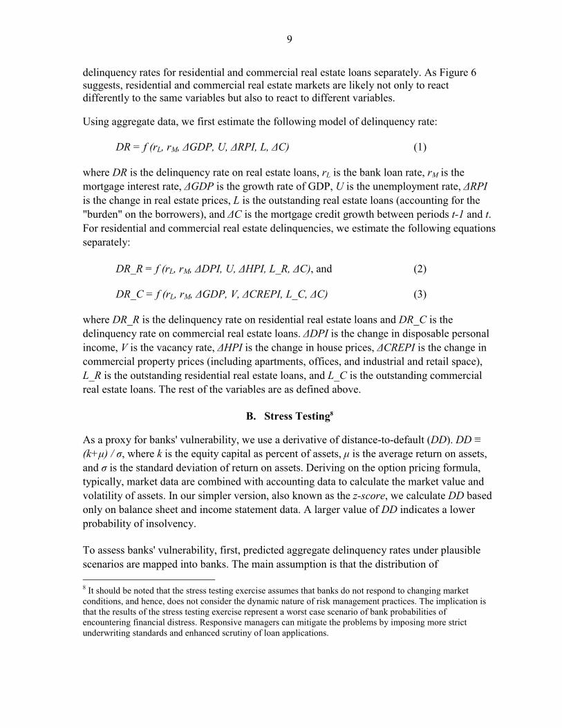
delinquency rates for residential and commercial real estate loans separately. As Figure 6 suggests, residential and commercial real estate markets are likely not only to react differently to the same variables but also to react to different variables.

Using aggregate data, we first estimate the following model of delinquency rate: DR = f (rL, rM, ΔGDP, U, ΔRPI, L, ΔC) (1) where DR is the delinquency rate on real estate loans, rL is the bank loan rate, rM is the mortgage interest rate, ΔGDP is the growth rate of GDP, U is the unemployment rate, ΔRPI is the change in real estate prices, L is the outstanding real estate loans (accounting for the "burden" on the borrowers), and ΔC is the mortgage credit growth between periods t-1 and t. For residential and commercial real estate delinquencies, we estimate the following equations separately: DR_R = f (rL, rM, ΔDPI, U, ΔHPI, L_R, ΔC), and (2) DR_C = f (rL, rM, ΔGDP, V, ΔCREPI, L_C, ΔC) (3) where DR_R is the delinquency rate on residential real estate loans and DR_C is the delinquency rate on commercial real estate loans. ΔDPI is the change in disposable personal income, V is the vacancy rate, ΔHPI is the change in house prices, ΔCREPI is the change in commercial property prices (including apartments, offices, and industrial and retail space), L_R is the outstanding residential real estate loans, and L_C is the outstanding commercial real estate loans. The rest of the variables are as defined above.

B. Stress Testing8

As a proxy for banks' vulnerability, we use a derivative of distance-to-default (DD). DD ≡ (k+μ) / σ, where k is the equity capital as percent of assets, μ is the average return on assets, and σ is the standard deviation of return on assets. Deriving on the option pricing formula, typically, market data are combined with accounting data to calculate the market value and volatility of assets. In our simpler version, also known as the z-score, we calculate DD based only on balance sheet and income statement data. A larger value of DD indicates a lower probability of insolvency. To assess banks' vulnerability, first, predicted aggregate delinquency rates under plausible scenarios are mapped into banks. The main assumption is that the distribution of 8 It should be noted that the stress testing exercise assumes that banks do not respond to changing market conditions, and hence, does not consider the dynamic nature of risk management practices. The implication is that the results of the stress testing exercise represent a worst case scenario of bank probabilities of encountering financial distress. Responsive managers can mitigate the problems by imposing more strict underwriting standards and enhanced scrutiny of loan applications.

10

delinquencies across banks remains unchanged. An example could help illustrate this point. Suppose there are two banks in the system, A and B, where bank A has 5 delinquent loans out of 50 and bank B has 20 delinquent loans out of 100. Hence, bank A and B have 10 and 20 percent delinquency rates, respectively, and the aggregate delinquency rate is 16.6 percent (25/150). If the aggregate delinquency rate was to increase to 20 percent, the delinquency rate in bank A would increase to 12 percent and that in bank B would become 24 percent, keeping the ratio of delinquencies in bank A to those in bank B at its original level (1 to 2). Once the mapping is completed, we recalculate DD assuming that the increase in delinquencies would decrease income from loans proportionately. The change in DD indicates how much closer the bank is to insolvency as a consequence of the increase in the delinquency rate. This allows us to split the banks into several categories depending on their response to specific macro shocks, allowing us to determine which banks are more at risk.

C. Determinants of Vulnerability

The final part in our approach builds on the last idea discussed in step 2, i.e., pinpointing which characteristics are more important to determine exposure to risk. This part is more concerned with policy implications and looks into how the change in distance to default depends on bank characteristics, such as size, geographic location, and other exposures. Hence, we look at the following regression equation using bank-level data: ΔDDi = g (Si, CIi, NIMi, LDi, LOCi, REi) (4) where S is the bank size (measured as log of total assets), CI is the cost-to-income ratio, NIM is the net interest margin, LD is the loan-to-deposit ratio, LOC is the location (to capture state-specific shocks) and RE is the percentage of loans that are related to real estate. This is a cross-section analysis where the dependent variable is the estimated change in distance to default (from step 2) and the independent variables are historical averages. Finally, we also use a panel data model to enhance our understanding of the determinants of the delinquency rate in real estate loans, DR, defined as (RealEstateNonperformingLoans+RealEstateNonaccruals)/(TotalRealEstateLoans), at the bank level. This analysis uses DR as its dependent variable and the same independent variables as the cross-section analysis described above, but now we use both year-to-year and cross-sectional variation and we introduce a time-fixed-effect and a measure of individual banks' credit growth. Hence, the regression equation to be estimated using panel data is DRit = h (Sit, CIi,t-1, NIMi,t-1, LDi,t-1, REi,t-1, LOCi, CGit, TFEt) (5) where TFE is the time-fixed-effect (to capture common movements), CG is the credit growth in bank i from period t-1 to t and other variables are essentially as defined above (keeping in mind that we no longer use averages).

11

These models allow us to understand where regulation should be directed, i.e., what the main determinants of exposure to real estate risk are and what type of regulations could be more effective. Thus, they enable us to provide an assessment of the proposed regulations.

IV. DATA

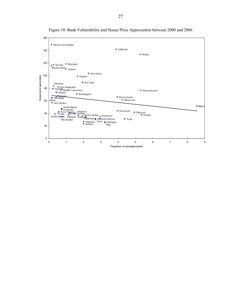
We utilize both macro and micro data at quarterly frequency. In the first and second steps, aggregate data compiled by federal agencies are used. The macroeconomic data for the analysis come from IMF International Financial Statistics database. These steps examine the relationship between aggregate delinquency rates and major economic factors during 1987-2006. The final step of the study relies on detailed bank accounting data to examine the loan composition and structure for U.S. banks from 1986 to 2006. The main data source is the Report of Condition and Income database (Call Report Files) that provides the balance sheets and income statements for all banks regulated by the Federal Reserve System. Breakdowns of loans in non-accrual status and information on nonperforming loans are used to compute the delinquency rate at the bank level. Following the discussion in the previous section, we model the decision to go delinquent on a loan as a function of interest rates, income, real estate prices, and credit conditions. Here, interest rates, income, and outstanding loans, proxing for debt burden, represent the factors affecting the borrower’s ability to pay. Inclusion of bank credit pertains to another aspect of payment capacity, namely, the ease of credit in the financial system, which is important when refinancing is offered as an option to delinquency. Real estate prices reflect the possibility of strategic default. As mentioned earlier, residential and commercial real estate loans are analyzed separately and factors that are likely to be more relevant for each type are employed as explanatory variables. For instance, while unemployment is linked to delinquencies in residential real estate loans, vacancy rate is a better proxy for economic activity related to delinquencies in commercial real estate loans. As for the bank-level analysis in step 3, we use CAMEL measures as determinants of bank soundness and control for bank characteristics such as size, growth, and exposure to real estate.9 Table 1 explains the variables used in the analysis while Table 2 presents the summary statistics.

9 CAMEL is a rating system used widely by bank supervisors. The main idea is assigning a score to each bank based on five factors: capital adequacy, asset quality, management, earnings, and liquidity. Lately, a sixth factor, sensitivity to market risk, was added, changing the acronym to CAMELS. For more information on CAMEL(S), see, among others, Lopez (1999).

12

V. RESULTS

A. What Leads to Delinquencies?

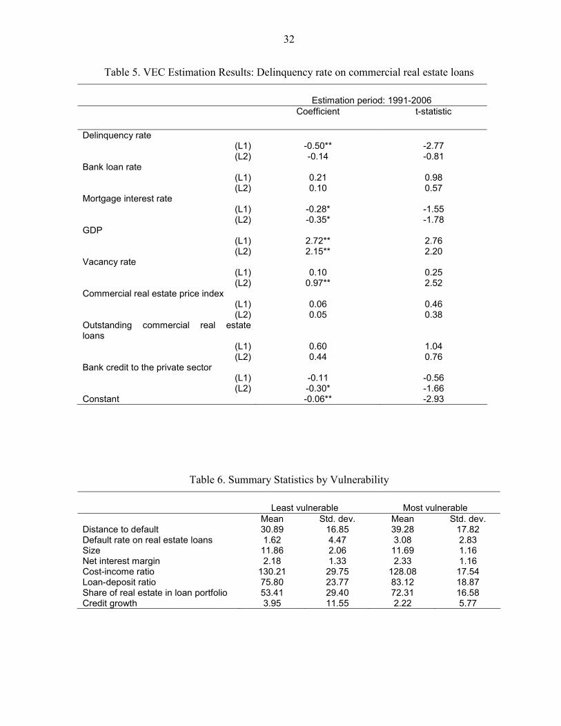
To find out which factors have the largest impact on aggregate delinquency rates while taking the feedback effect between the credit and real estate cycles into account, we use a vector error correction framework.10 Table 3 presents the estimates for aggregate delinquency rates on all real estate loans while Tables 4 and 5 show the results for residential and commercial real estate loans separately. Based on these estimation results, we plot the impulse response functions demonstrating the accumulated impact of a one standard deviation change in the variable of interest on the delinquency rate. Figure 7 shows that real estate loan delinquencies are most likely to be driven by changes in the mortgage interest rate and real estate prices, in line with Elmer and Seelig (1999). Overall delinquency rates on real estate loans respond strongly to changes in mortgage interest rates, yet, as expected, delinquency behavior for residential real estate and commercial real estate loans differ considerably. In particular, residential real estate loans are more sensitive to interest rate changes as well as to changes in household income and unemployment rates reflecting the arguments set forth in the ability to pay hypothesis. While rising mortgage interest rates lead to an increase in delinquencies as more borrowers find it harder to make their payments, an increasing house price also appear to be linked to a higher delinquency rate. Looking at residential and commercial delinquency rates separately, however, reveals that rising property prices are negatively related to delinquencies on commercial real estate loans (Figures 8 and 9). Commercial real estate loans also appear to come under pressure on the face of increased debt burden and movements in the business cycle, as demonstrated in the delinquency rate’s response to GDP and vacancy rates. These results suggest that the delinquencies on commercial real estate loans can be better explained by strategic behavior, as suggested by Vandel et al (1993), whereas the positive relation between (residential) house prices and delinquency rate is inconsistent with the strategic default hypothesis, in contrast to Quigley et al (2000). A potential explanation for this, nevertheless, could be households borrowing beyond their means.

10 Before proceeding with the regression analysis, we check if the data series we are using are stationary. All series are found to be I(1) at high levels of significance, with the slight exception of outstanding commercial real estate loans, for which the null hypothesis of the first difference having a unit root is rejected at the 10 percent significance level. Then, we determine the number of cointegrating relationships. The test statistics support the existence of two cointegrating relationships for real estate loans at the 5 percent significance level. For residential and commercial real estate loans, the number of cointegrating relationships are one and three, respectively. Tables summarizing the unit root and Johansen cointegration tests are available on request.

13

B. Can the Banking Sector Survive an Economic Downturn?

Findings from the first step of our analysis suggest that mortgage interest rates are important in determining delinquency rates on real estate loans. Specifically, a one standard deviation increase in the mortgage interest rate could trigger a 1.1 percentage point accumulated increase in the real estate loan delinquency rate over 4 years. Since interest rates can be taken as an indicator of other changes in the economy, we treat an increase in interest rates as the sign of economically hard times and calculate the impact on the average real estate loan portfolio.11 Increase in interest rates might curb demand for home purchase loans and initiate a slowdown in house price appreciation; hence, looking at the impact of higher interest rates could shed light on the consequences of a glum real estate market. This stress-testing exercise also encompasses the potential effects of resetting interest rates on adjustable-rate mortgages. A typical bank in 2006, with a delinquency rate of 2.0 percent and real estate share of 66.6 percent in its loan portfolio, would suffer an interest income drop equal to 10.3 percent were the delinquency rate to experience a 1.1 percentage point increase and rise to 3.1 percent. This would correspond to a 20 percent decrease in the bank’s distance to default, indicating an increased likelihood of solvency problems. One could interpret these average figures as justification for a widespread regulatory move on commercial banks’ real estate lending activities. On a bank-by-bank basis, however, less than 1 percent of the banks carry the risk of becoming insolvent, i.e., distance to default measure entering the negative territory. Four-fifths of the these banks have exposure to real estate in their loan portfolios in excess of the sample average of 66.6 percent and three-fourths of them have exposure exceeding the median value of 70.84 percent. These indicate a high degree of asymmetry between vulnerable and sound banks in terms of their exposure to real estate.12 To explore these issues further and evaluate the merits of an industry-wide regulation, we look into the differences across banks depending on the estimated response of the distance to default measure to the change in interest rates.

C. Who are the Vulnerable Banks?

Table 6 shows the summary statistics for the least and most vulnerable banks, where the least and most vulnerable banks are defined by the top and bottom quintiles with respect to the

11 Higher interest rates here imply decreased ability to make payments because cost of borrowing is higher. This might occur, for instance, as economic activity reaches its peak and monetary stance tightens.

12 Summary statistics also point to a great degree of skewness in the distribution of key variables across banks. For instance, while the median delinquency rate stands at 2 percent, the mean is closer to 4 percent. Hence, it is possible that a small number of banks find themselves in serious distress, potentially spreading the problems elsewhere in the financial system through cross holdings.

14

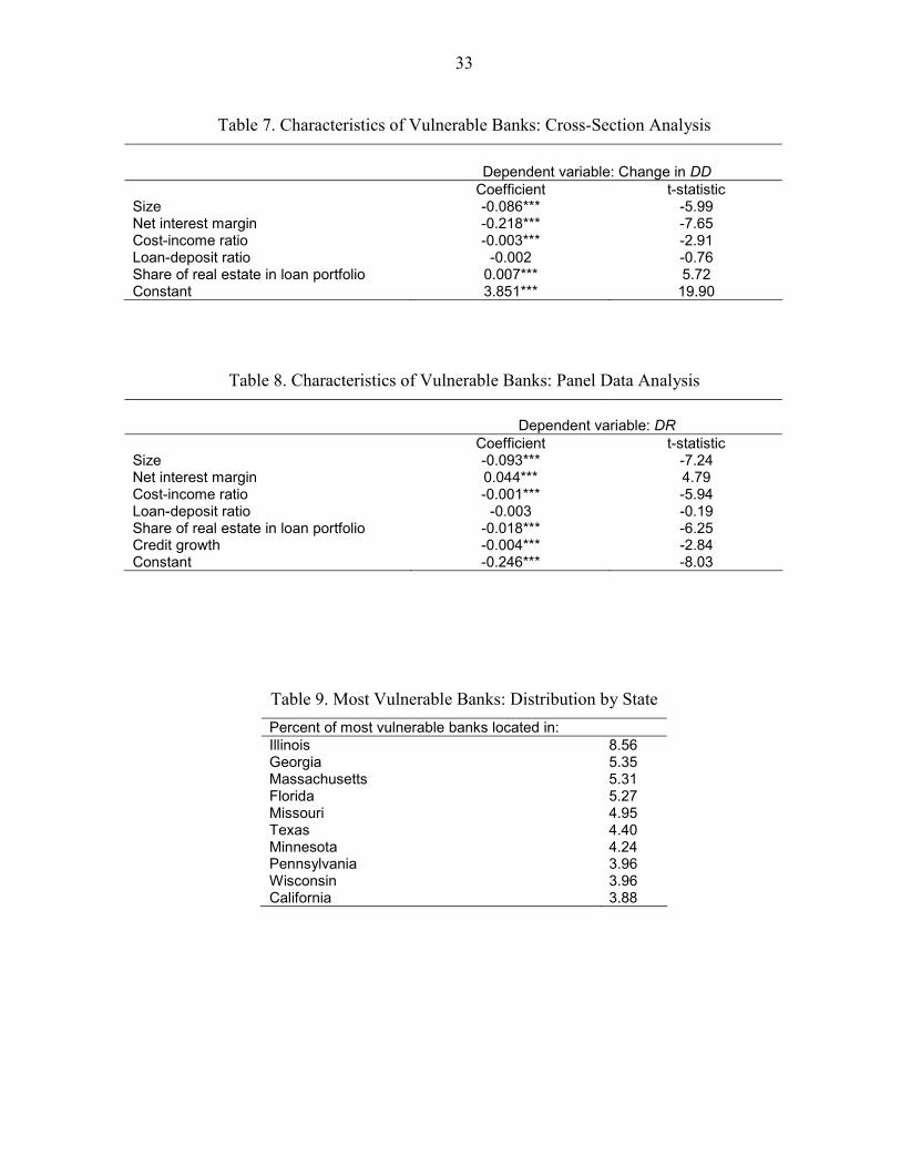
change in the distance to default measure. It appears to be the case that banks with high loan-deposit ratios and large share of real estate loans in their lending activities are more likely to be among the most vulnerable. Next, we investigate whether these characterizations remain valid in the regression analysis. Table 7 shows the results of estimating the cross-sectional equation ΔDDi = α + β1Si + β2CIi + β3NIMi + β4LDi + β5REi + β6LOCi + εi (6) while Table 8 presents the results of estimating the panel data equation DRit = α + β1Sit + β2CIi,t-1 + β3NIMi,t-1 + β4LDi,t-1 + β5REi,t-1 + β6CGit (7) + γ1 LOCi + γ2TFEt + εit where coefficients on location and time dummies are suppressed for sake of brevity. These regression results partially confirm the picture that emerges from examining the summary statistics. The small difference between the average size of least and most vulnerable banks is apparently not statistically significant. Actually, larger banks have a higher likelihood of facing troubles in the event of an economic downturn, which is somewhat puzzling at first sight because they tend to have lower delinquency rates on their real estate loans. Yet, further investigation of the relation between size and delinquency rates reveal that delinquency rates increase more in the case of an economic downturn in larger banks. In the cross-sectional regressions, banks with high net interest margins, although profitable, appear to be more vulnerable to shocks brought about by changes in the interest rates both through the direct impact and through the indirect impact of increased delinquency rates triggered by the higher interest rates. Panel data regressions suggest that this could be because these banks take on riskier loans as they tend to have relatively more delinquent real estate loans. Less efficient banks, as indicated by the coefficient on cost-income ratio in Table 8, would experience a sharper drop in their distance to default although they do not necessarily have higher rates of delinquent loans in their real estate portfolios, as seen in Table 9. This points out the importance of management quality and the associated enhanced efficiency. Banks that have high shares of real estate loans in their portfolio, probably because they tend to have a relatively lower proportion of nonperforming real estate loans, do not appear to be more vulnerable. One potential explanation for this seemingly puzzling finding is that these banks have relatively more income from other activities that could offset the downfall in income from their real estate loan portfolios. Alternatively, one could argue that these banks choose to “specialize” in real estate lending because they have an ability to make better loans in this market, and hence, a lower rate of delinquency. If they are also good at managing the associated risks, then they will not appear to be any more vulnerable than banks that do not specialize in real estate lending. Finally, banks that extend credit faster tend to have higher real estate loan delinquency rates, which points out to aggressive lending practices during phases of rapid credit expansion.

15

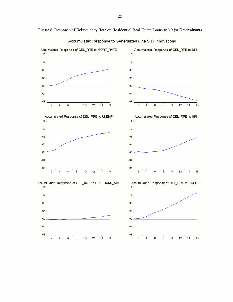
Location also could be an important factor as real estate loans are particularly sensitive to local housing market conditions. Table 9 gives a list of the top ten states in the distribution of the most vulnerable banks across states.13 It is interesting to notice that some of these states, such as Florida and California, have been among the places experiencing stronger real estate price booms than others in the past few years. Figure 10 illustrates this insight further. Hence, the event of downturn in the housing cycle might have a higher probability of happening in these states where house price appreciation has been higher, making the borrowers and the lenders more vulnerable.

D. What is the Likely Impact of Recent Regulations?

Supervisory and regulatory policy discussions at the end of 2006 and the beginning of 2007 focused on commercial real estate exposure and the potential risks associated with nontraditional mortgage loans. Looking at the composition of real estate loans in banks’ portfolios, it is hard to argue concentration in commercial real estate loans poses an immediate concern. Relative share of commercial real estate loans has been stable while the increase in banks’ exposure to real estate has been driven by an increased share of residential real estate loans. Moreover, the gap between commercial and residential real estate loans in terms of level and volatility of delinquency rates has narrowed in the past decade. Hence, given the increasing concentration in residential real estate loans and converging risk profile of this type of loans, the concern on the use of nontraditional mortgage products to expand residential real estate loan portfolios appear to be quite relevant. That said, our analysis also reveals that there is considerable variation on the extent of exposure among banks. Therefore, more refined measures such as intensified supervision of most vulnerable banks and guidance targeted on specific risk factors would be preferable. In particular, given the importance of mortgage interest rates and the expanding use of adjustable-rate mortgages in riskier segments of the borrower pool, supervisors should encourage sound risk management practices regarding such products and closely monitor the status of those institutions which use such products more frequently.14

VI. CONCLUSION

In the five years to March 2007, house prices grew at an annual rate of 8 percent while outstanding mortgage debt almost doubled. In residential versus commercial comparison, it

13 For banks operating in multiple states, the data are rearranged at the state level. For example, Wachovia appears as several entities in the database as Wachovia California and Wachovia Arizona. Therefore, the location variable reflects the situation associated with the location of the loan activity and/or property.

14 An equally important development in mortgage markets has been the increased degree of securitization. The analysis here focuses on the traditional measures of exposure while supervisors should also watch the exposure through asset-backed security holdings.

16

was the residential real estate prices and real estate loans contributing more to the overall growth. Share of real estate-related loans in the same period increased from 42.6 percent to 56.5 percent where subprime lending at nontraditional terms was the fastest growing segment of the residential mortgage market. The analysis conducted here using information on commercial banks' balance sheets right before the financial crisis of 2007-08 stormed the economy suggest that not all banks had the capacity to absorb the consequences of potential adverse movements in interest rates and house prices. Vulnerable banks tend to expand loans rapidly, have poor efficiency records and high real estate lending activity levels, and those located in a number of states some of which had experienced a house price boom. While it may come as no surprise that inefficient banks are more likely to run into trouble, we identify another generally-overlooked characteristic, namely, the rate of loan growth, as an indicator of vulnerability. In the light of the events that took down some institutions in 2007 and 2008, it appears to be the case that there were some vulnerability pockets that could have been detected back in 2006.

17

REFERENCES Archer, W. R., P. J. Elmer, D. M. Harrison, and D. C. Ling, 1998, “Determinants of

Multifamily Mortgage Default,” FDIC Working Paper No. 99–2. Asea, P. K., and B. Blomberg, 1998, “Lending Cycles,” Journal of Econometrics, Vol. 83,

pp. 89–123. Avery, R., R. Bostic, P. Calem, and G. Canner, 1996, “Credit Risk, Credit Scoring, and the Performance of Home Mortgages,” Federal Reserve Bulletin. Vol. 82, pp. 621–64. Ball, M. T. Morrison, and A. Wood, 1996, “Structures Investment and Economic Growth,”

Urban Studies, Vol. 33, pp.1687–706. Ball, M., and A. Wood, 1999, “Housing Investment: Long-Run International Trends and Volatility,” Housing Studies, Vol.14, pp.185–209. Bank of International Settlements - BIS, 2001, 71st Annual Report, Washington, .D.C. Elmer, P. J., and S. A. Seelig, 1999, “Insolvency, Trigger Events, and Consumer Risk

Posture in the Theory of Single-Family Mortgage Default,” FDIC Working Paper No. 98–3.

International Monetary Fund, 2000, World Economic Outlook (May) Washington, D.C. Jimenez, G., and J. Saurina, 2006, “Credit Cycles, Credit Risk, and Prudential Regulation,”

International Journal of Central Banking, Vol. 2, pp. 65–97. Kiyotaki, N., and J. Moore, 1997, “Credit Cycles,” Journal of Political Economy, Vol.105,

pp. 211–48. Lopez, J. A., 1999, “Using CAMELS Ratings to Monitor Bank Conditions,” FRBSF Economic Letter, pp. 99–19. Ruckes, M., 2004, “Bank Competition and Credit Standards,” Review of Financial Studies, Vol. 17, pp.1073–102. Quigley, J. M., R. Van Order, and Y. Deng, 2000, “Mortgage Terminations, Heterogeneity and the Exercise of Mortgage Options,” Econometrica, Vol. 68, pp. 275–307. Vandell, K. D., W. Barnes, D. Hartzell, D. Kraft, and W. Wendt, 1993, “Commercial Mortgage Defaults: Proportional Hazards Estimation Using Individual Loan Histories,” AREUEA Journal, Vol. 21, pp. 451–80.

18

Figure 1. Business, Credit, and Real Estate Cycles, 1976-2006

-15

-10

-5

0

5

10

15

20

1976Q1 1982Q1 1988Q1 1994Q1 2000Q1 2006Q1

GDP growth

Credit growth

Returns to housing

Sources: IMF International Financial Statistics, Office of Federal Housing Enterprise Oversight.

19

Figure 2. Share of All Real Estate-Related Loans in Banks' Portfolio, 1960-2006

0

10

20

30

40

50

60

60-Q1 63-Q1 66-Q1 69-Q1 72-Q1 75-Q1 78-Q1 81-Q1 84-Q1 87-Q1 90-Q1 93-Q1 96-Q1 99-Q1 02-Q1 05-Q1

RE loans

Source: Haver Analytics.

20

Figure 3. Share of Real Estate Loans in Banks' Portfolio, 1996-2006

0

10

20

30

40

50

60

1996Q4 1997Q3 1998Q2 1999Q1 1999Q4 2000Q3 2001Q2 2002Q1 2002Q4 2003Q3 2004Q2 2005Q1 2005Q4 2006Q3

Commercial Residential

Source: Haver Analytics.

21

Figure 4. Real Estate Price Indices, 1984-2006

Figure 3. Real Estate Price Indices

0

20

40

60

80

100

120

140

160

180

84-Q1 87-Q1 90-Q1 93-Q1 96-Q1 99-Q1 02-Q1 05-Q1

Commercial

Residential

Source: Haver Analytics.

22

Figure 5. Real Estate Exposure: Median Bank, 2000-2006

Source: Federal Reserve Report of Condition and Income database.

35

40

45

50

2000q1 2000q3 2005q1 2005q3 2006q1 2006q3

RE loans and MBS(in percent of total assets)

380

430

480

2000q1 2000q3 2005q1 2005q3 2006q1 2006q3

RE loans and MBS(in percent of equity capital)

1.5

2

2.5

3

3.5

4

2000q1 2000q3 2005q1 2005q3 2006q1 2006q3

Unused RE loan commitments(in percent of total assets)

15

20

25

30

35

40

2000q1 2000q3 2005q1 2005q3 2006q1 2006q3

Unused RE loan commitments(in percent of equity capital)

9

9.5

10

10.5

2000q1 2000q2 2000q3 2000q4 2005q1 2005q2 2005q3 2005q4 2006q1 2006q2 2006q3 2006q4

Equity capital(in percent of total assets)

23

Figure 6. Delinquency Rate, 1991-2006

Source: Federal Reserve.

0

2

4

6

8

10

12

14

1991Q1 1991Q4 1992Q3 1993Q2 1994Q1 1994Q4 1995Q3 1996Q2 1997Q1 1997Q4 1998Q3 1999Q2 2000Q1 2000Q4 2001Q3 2002Q2 2003Q1 2003Q4 2004Q3 2005Q2 2006Q1

All loans

0

2

4

6

8

10

12

14

1991Q1 1992Q3 1994Q1 1995Q3 1997Q1 1998Q3 2000Q1 2001Q3 2003Q1 2004Q3 2006Q1

Business loans

Loans secured by real estate

Consumer loans

0

2

4

6

8

10

12

14

1991Q1 1992Q3 1994Q1 1995Q3 1997Q1 1998Q3 2000Q1 2001Q3 2003Q1 2004Q3 2006Q1

Loans secured by real estate

Residential real estate

Commercial real estate

24

Figure 7. Response of Delinquency Rate on Real Estate Loans to Major Determinants

-.08

-.04

.00

.04

.08

.12

.16

.20

2 4 6 8 10 12 14 16

Accumulated Response of DEL_RE to PRIME_RATE

-.08

-.04

.00

.04

.08

.12

.16

.20

2 4 6 8 10 12 14 16

Accumulated Response of DEL_RE to MORT_RATE

-.08

-.04

.00

.04

.08

.12

.16

.20

2 4 6 8 10 12 14 16

Accumulated Response of DEL_RE to GDP

-.08

-.04

.00

.04

.08

.12

.16

.20

2 4 6 8 10 12 14 16

Accumulated Response of DEL_RE to RPI

-.08

-.04

.00

.04

.08

.12

.16

.20

2 4 6 8 10 12 14 16

Accumulated Response of DEL_RE to RELOANS_AVE

-.08

-.04

.00

.04

.08

.12

.16

.20

2 4 6 8 10 12 14 16

Accumulated Response of DEL_RE to CREDIT

Accumulated Response to Cholesky One S.D. Innovations

25

Figure 8. Response of Delinquency Rate on Residential Real Estate Loans to Major Determinants

-.08

-.04

.00

.04

.08

.12

.16

2 4 6 8 10 12 14 16

Accumulated Response of DEL_RRE to MORT_RATE

-.08

-.04

.00

.04

.08

.12

.16

2 4 6 8 10 12 14 16

Accumulated Response of DEL_RRE to DPI

-.08

-.04

.00

.04

.08

.12

.16

2 4 6 8 10 12 14 16

Accumulated Response of DEL_RRE to UNEMP

-.08

-.04

.00

.04

.08

.12

.16

2 4 6 8 10 12 14 16

Accumulated Response of DEL_RRE to HPI

-.08

-.04

.00

.04

.08

.12

.16

2 4 6 8 10 12 14 16

Accumulated Response of DEL_RRE to RRELOANS_AVE

-.08

-.04

.00

.04

.08

.12

.16

2 4 6 8 10 12 14 16

Accumulated Response of DEL_RRE to CREDIT

Accumulated Response to Generalized One S.D. Innovations

26

Figure 9. Response of Delinquency Rate on Commercial Real Estate Loans to Major Determinants

-.15

-.10

-.05

.00

.05

.10

.15

.20

2 4 6 8 10 12 14 16

Accumulated Response of DEL_CRE to PRIME_RATE

-.15

-.10

-.05

.00

.05

.10

.15

.20

2 4 6 8 10 12 14 16

Accumulated Response of DEL_CRE to GDP

-.15

-.10

-.05

.00

.05

.10

.15

.20

2 4 6 8 10 12 14 16

Accumulated Response of DEL_CRE to VAC

-.15

-.10

-.05

.00

.05

.10

.15

.20

2 4 6 8 10 12 14 16

Accumulated Response of DEL_CRE to CREPI

-.15

-.10

-.05

.00

.05

.10

.15

.20

2 4 6 8 10 12 14 16

Accumulated Response of DEL_CRE to CRELOANS_AVE

-.15

-.10

-.05

.00

.05

.10

.15

.20

2 4 6 8 10 12 14 16

Accumulated Response of DEL_CRE to CREDIT

Accumulated Response to Generalized One S.D. Innovations

27

Figure 10. Bank Vulnerability and House Price Appreciation between 2000 and 2006

Alabama

Arizona

Arkansas

California

Colorado

Connecticut

Delaware

District of Columbia

Florida

Georgia

Idaho

Illinois

IndianaIowa

KansasKentucky

Louisiana

Maine

Maryland

Massachusetts

Michigan

Minnesota

Mississippi

Missouri

Montana

Nebraska

Nevada

New Hampshire

New Jersey

New Mexico

New York

North Carolina

North Dakota

Ohio

Oklahoma

Oregon

Pennsylvania

Rhode Island

South CarolinaSouth Dakota Tennessee

Texas

Utah

Vermont

Virginia

Washington

West Virginia Wisconsin

Wyoming

0

20

40

60

80

100

120

140

160

0 1 2 3 4 5 6 7 8 9

Proportion of vulnerable banks

Hou

se p

rice

appr

ecia

tion

28

Table 1. Definition and Source of Variables

Variable Definition Source Aggregate: Delinquency rate Loans secured by real estate that are past due

thirty days or more and still accruing interest as well as those in nonaccrual status, expressed as a percentage of end-of-period loans (available separately for residential and commercial real estate)

FFIEC

Mortgage interest rate Contract interest rate on commitments for fixed-rate first mortgages

FHLMC

Bank loan rate Rate posted by a majority of top 25 (by assets in domestic offices) insured U.S.-chartered commercial banks

FED

Disposable personal income Personal income less personal current taxes BEA GDP Gross domestic product IFS Unemployment Unemployment rate IFS Vacancy rate Proportion of real estate inventory which is vacant

for industrial, office, or residential rental use BC

Bank credit to the private sector Loans extended to private corporations and individuals by commercial banks

IFS

Outstanding real estate loans Stock of real estate-related loans (available separately for residential and commercial real estate)

FED

Real estate price index Transaction-based prices of real estate properties (available separately for residential and commercial real estate)

OFHEO†

Bank level: Distance to default Sum of equity capital and return on assets divided

by return volatility, calculated on a rolling basis FED††

Size Logarithm of total bank assets FED†† Net interest margin Difference between interest expense and interest

income, expressed as a percentage of average earning assets

FED††

Cost-income ratio Total costs divided by total income FED†† Loan-deposit ratio Total loans divided by total deposits FED†† Share of real estate in loan portfolio Loans secured by real estate divided by total

loans (available separately for residential and commercial real estate)

FED††

Credit growth Growth rate of total real estate loans (available separately for residential and commercial real estate)

FED††

Abbreviations: FFIEC - Federal Financial Institutions Examination Council; FHLMC - Federal Home Loan Mortgage Corporation; FED - Federal Reserve Board; BEA - Bureau of Economic Analysis; IFS - IMF International Financial Statistics; BC - Bureau of the Census; OFHEO - Office of Federal Housing Enterprise Oversight. † Authors’ calculations using the single-family home price index by OFHEO and commercial real estate transaction-based price index constructed by MIT Center for Real Estate †† Authors’ calculations using the Report of Condition and Income database maintained by Chicago FED

29

Table 2. Summary Statistics

Variable Mean Std. dev.Aggregate:

Delinquency rate on all real estate loans 3.58 0.24Delinquency rate on residential real estate loans 2.85 0.25Delinquency rate on commercial real estate loans 2.73 0.48Mortgage interest rate 2.05 0.19Bank loan rate 1.99 0.28Disposable personal income 8.68 0.30GDP 9.07 0.14Unemployment 1.70 0.17Vacancy rate 2.29 0.12Bank credit to the private sector 9.43 0.32Outstanding real estate loans 7.07 0.50Outstanding residential real estate loans 6.44 0.57Outstanding commercial real estate loans 6.20 0.45Real estate price index 5.05 0.24Residential real estate price index 5.37 0.28Commercial real estate price index 4.73 0.22Bank level:

Distance to default 33.63 16.30Size 11.69 1.45Net interest margin 2.31 1.20Cost-income ratio 130.51 21.78Loan-deposit ratio 78.69 20.46Share of real estate in loan portfolio 62.40 22.09Share of residential real estate in loan portfolio 28.88 19.38Share of commercial real estate in loan portfolio 21.80 15.93Credit growth in real estate loans 3.40 8.89Credit growth in residential real estate loans 2.67 10.10Credit growth in commercial real estate loans 4.30 12.00Note: All aggregate data series are seasonally adjusted and are in logs.

30

Table 3. VEC Estimation Results: Delinquency rate on real estate loans

Estimation period: 1987-2006 Coefficient t-statistic

Delinquency rate (L1) -0.20* -1.61 (L2) -0.07 -0.60

Bank loan rate (L1) -0.03 -0.34 (L2) 0.07 0.81

Mortgage interest rate (L1) -0.04 -0.36 (L2) -0.001 -0.01

GDP (L1) -0.34 -0.87 (L2) -0.39 -0.95

Real estate price index (L1) -0.01 -0.08 (L2) 0.30** 2.63

Outstanding real estate loans (L1) 0.16 0.63 (L2) 0.03 0.14

Bank credit to the private sector (L1) -0.17* -1.94 (L2) -0.08 -0.91

Constant -0.002 0.31

31

Table 4. VEC Estimation Results: Delinquency rate on residential real estate loans Estimation period: 1991-2006 Coefficient t-statistic

Delinquency rate (L1) -0.39** -3.41 (L2) -0.16* -1.42

Bank loan rate (L1) -0.45** -3.66 (L2) 0.02 0.15

Mortgage interest rate (L1) -0.09 -0.80 (L2) -0.06 -0.38

Disposable personal income (L1) -0.60* -1.73 (L2) -0.83** -2.67

Unemployment (L1) -0.41*** -6.44 (L2) -0.24*** -4.69

Residential real estate price index (L1) 0.59* 1.58 (L2) 0.22 0.57

Outstanding residential real estate loans (L1) 0.10 0.48 (L2) -0.02 -0.12

Bank credit to the private sector (L1) -0.34*** -3.50 (L2) -0.19* -1.62

Constant 0.01* 1.46

32

Table 5. VEC Estimation Results: Delinquency rate on commercial real estate loans Estimation period: 1991-2006 Coefficient t-statistic

Delinquency rate (L1) -0.50** -2.77 (L2) -0.14 -0.81

Bank loan rate (L1) 0.21 0.98 (L2) 0.10 0.57

Mortgage interest rate (L1) -0.28* -1.55 (L2) -0.35* -1.78

GDP (L1) 2.72** 2.76 (L2) 2.15** 2.20

Vacancy rate (L1) 0.10 0.25 (L2) 0.97** 2.52

Commercial real estate price index (L1) 0.06 0.46 (L2) 0.05 0.38

Outstanding commercial real estate loans

(L1) 0.60 1.04 (L2) 0.44 0.76

Bank credit to the private sector (L1) -0.11 -0.56 (L2) -0.30* -1.66

Constant -0.06** -2.93

Table 6. Summary Statistics by Vulnerability Least vulnerable Most vulnerable Mean Std. dev. Mean Std. dev. Distance to default 30.89 16.85 39.28 17.82 Default rate on real estate loans 1.62 4.47 3.08 2.83 Size 11.86 2.06 11.69 1.16 Net interest margin 2.18 1.33 2.33 1.16 Cost-income ratio 130.21 29.75 128.08 17.54 Loan-deposit ratio 75.80 23.77 83.12 18.87 Share of real estate in loan portfolio 53.41 29.40 72.31 16.58 Credit growth 3.95 11.55 2.22 5.77

33

Table 7. Characteristics of Vulnerable Banks: Cross-Section Analysis Dependent variable: Change in DD Coefficient t-statistic Size -0.086*** -5.99 Net interest margin -0.218*** -7.65 Cost-income ratio -0.003*** -2.91 Loan-deposit ratio -0.002 -0.76 Share of real estate in loan portfolio 0.007*** 5.72 Constant 3.851*** 19.90

Table 8. Characteristics of Vulnerable Banks: Panel Data Analysis Dependent variable: DR Coefficient t-statistic Size -0.093*** -7.24 Net interest margin 0.044*** 4.79 Cost-income ratio -0.001*** -5.94 Loan-deposit ratio -0.003 -0.19 Share of real estate in loan portfolio -0.018*** -6.25 Credit growth -0.004*** -2.84 Constant -0.246*** -8.03

Table 9. Most Vulnerable Banks: Distribution by State Percent of most vulnerable banks located in: Illinois 8.56 Georgia 5.35 Massachusetts 5.31 Florida 5.27 Missouri 4.95 Texas 4.40 Minnesota 4.24 Pennsylvania 3.96 Wisconsin 3.96 California 3.88