extended kalman filter
DESCRIPTION
Day 25. Extended Kalman Filter. with slides adapted from http://www.probabilistic-robotics.com. Kalman Filter Summary. Highly efficient : Polynomial in measurement dimensionality k and state dimensionality n : O(k 2.376 + n 2 ) Optimal for linear Gaussian systems ! - PowerPoint PPT PresentationTRANSCRIPT
1
Extended Kalman FilterDay 25
with slides adapted from http://www.probabilistic-robotics.com
2
Kalman Filter Summary
• Highly efficient: Polynomial in measurement dimensionality k and state dimensionality n: O(k2.376 + n2)
• Optimal for linear Gaussian systems!
• Most robotics systems are nonlinear!
3
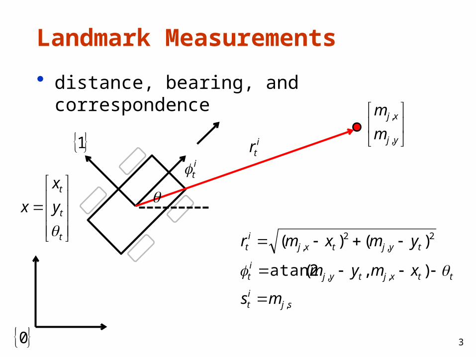
Landmark Measurements
• distance, bearing, and correspondence
1
0
t
t
t
y
x
x
yj
xj
m
m
,
,
it
itr
sjit
ttxjtyjit
tyjtxjit
ms
xmym
ymxmr
,
,,
2,
2,
),(atan2
)()(
4
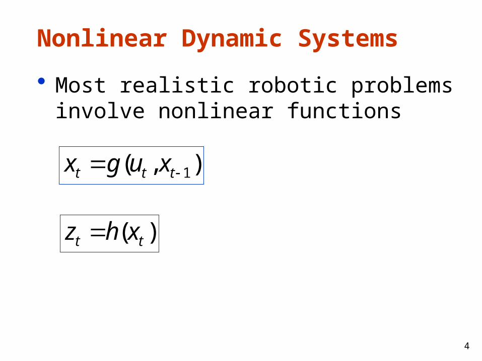
Nonlinear Dynamic Systems
• Most realistic robotic problems involve nonlinear functions
),( 1 ttt xugx
)( tt xhz

5
Nonlinear Dynamic Systems
• localization with landmarks
),( 1
)cos(cos
)sin(sin
tt
t
t
t
t
t
t
t
t
xug
t
tvv
tvv
t
t
ty
tx
x
),,(
,
,,
2,
2,
),(atan2
)()(
mjxh
sj
txjtyj
yjxj
z
it
it
it
t
it
m
xmym
ymxm
s
r
6
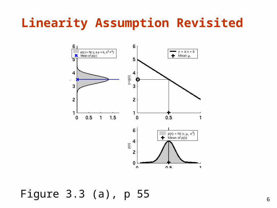
Linearity Assumption Revisited
Figure 3.3 (a), p 55
7
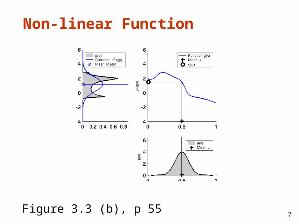
Non-linear Function
Figure 3.3 (b), p 55
8
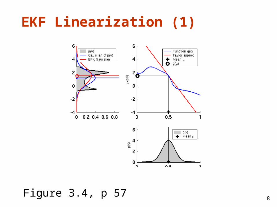
EKF Linearization (1)
Figure 3.4, p 57

9
EKF Linearization (2)
Figure 3.5 (a), p 62
10
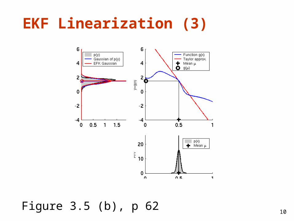
EKF Linearization (3)
Figure 3.5 (b), p 62

11
Taylor Series
• recall for f(x) infinitely differentiable around in a neighborhood a
• in the multidimensional case, we need the matrix of first partial derivatives (the Jacobian matrix)
))(()(
...)(!2
)()(
!1
)()()( 2
axafaf
axaf
axaf
afxf
12
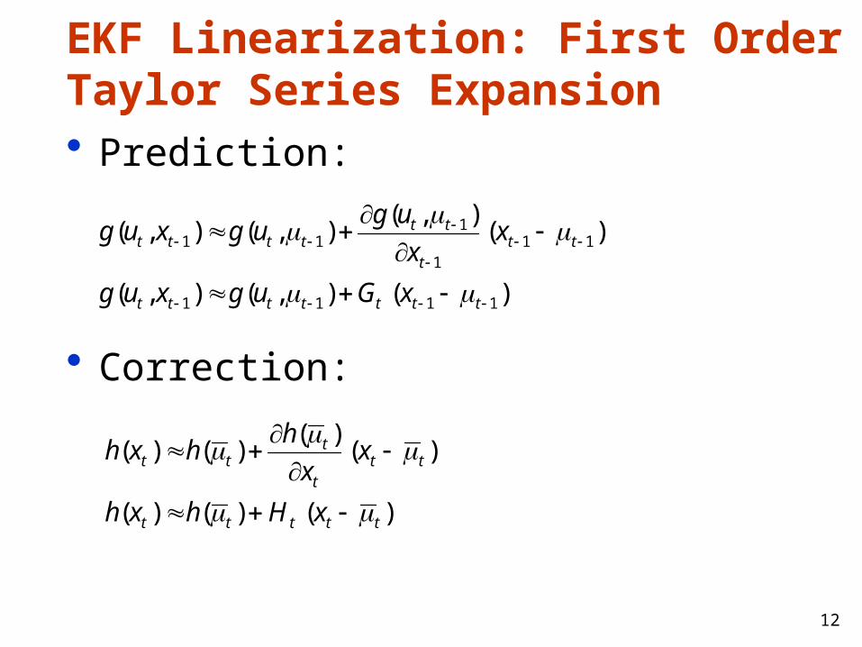
• Prediction:
• Correction:
EKF Linearization: First Order Taylor Series Expansion
)(),(),(
)(),(
),(),(
1111
111
111
ttttttt
ttt
tttttt
xGugxug
xx
ugugxug
)()()(
)()(
)()(
ttttt
ttt
ttt
xHhxh
xx
hhxh
13
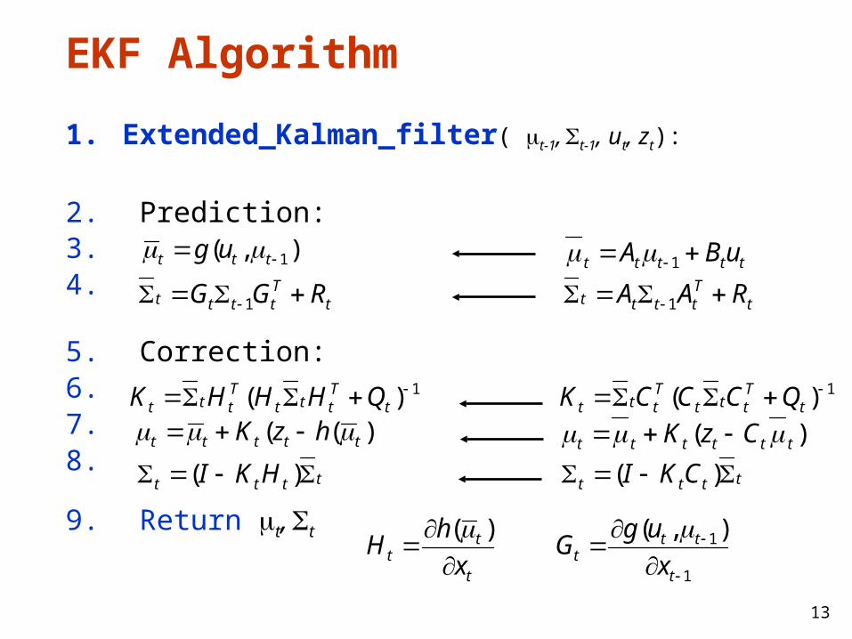
EKF Algorithm
1. Extended_Kalman_filter( mt-1, St-1, ut, zt):
2. Prediction:3. 4.
5. Correction:6. 7. 8.
9. Return t, St
),( 1 ttt ug
tTtttt RGG SS 1
1)( SS tTttt
Tttt QHHHK
))(( ttttt hzK
tttt HKI SS )(
1
1),(
t
ttt x
ugG
t
tt x
hH
)(
ttttt uBA 1
tTtttt RAA SS 1
1)( SS tTttt
Tttt QCCCK
)( tttttt CzK
tttt CKI SS )(
14
Localization
• Given • Map of the environment.• Sequence of sensor measurements.
• Wanted• Estimate of the robot’s position.
• Problem classes• Position tracking• Global localization• Kidnapped robot problem (recovery)
“Using sensory information to locate the robot in its environment is the most fundamental problem to providing a mobile robot with autonomous capabilities.” [Cox ’91]
15
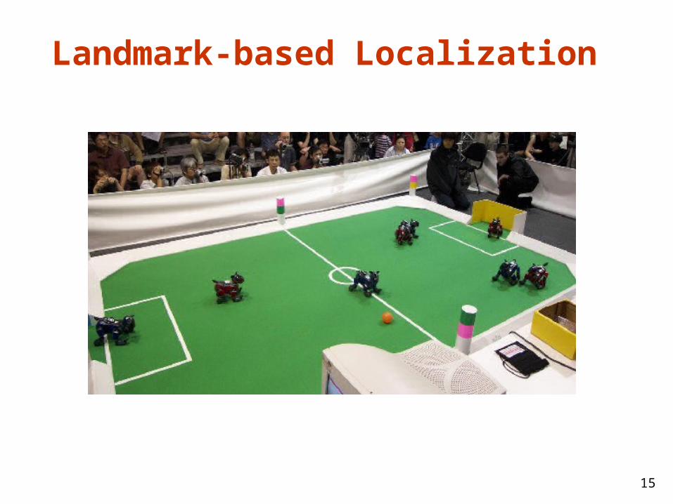
Landmark-based Localization
16
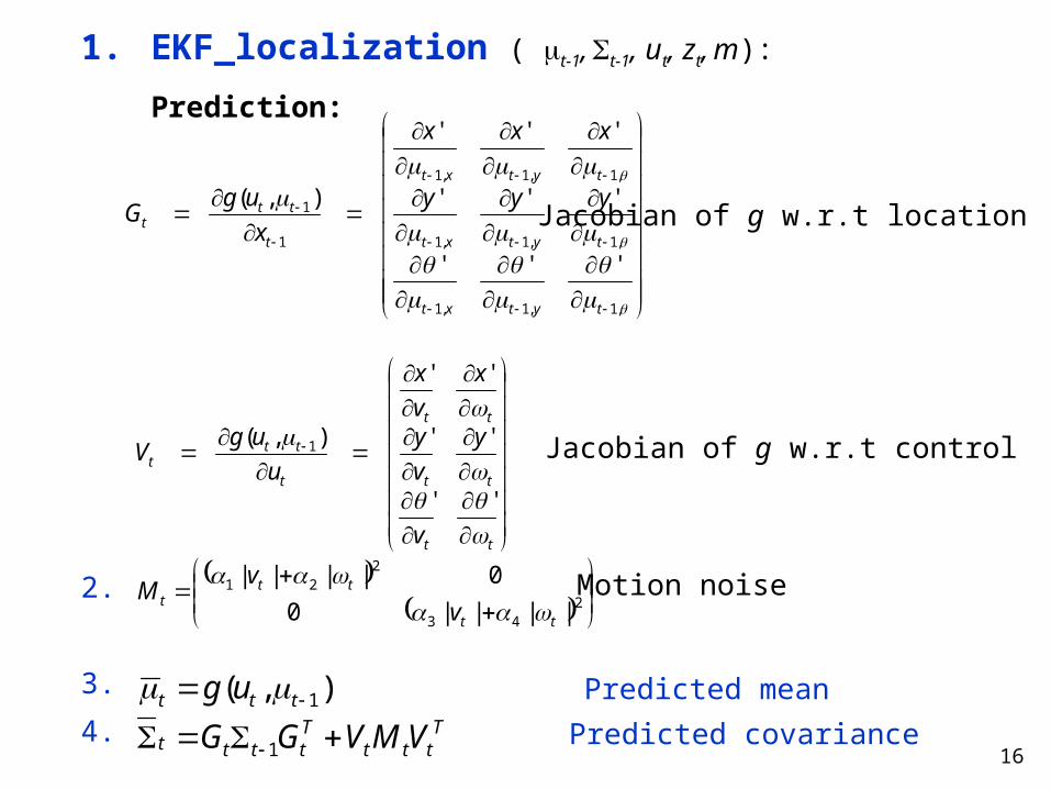
1. EKF_localization ( mt-1, St-1, ut, zt, m):
Prediction:
2.
3.
4. ),( 1 ttt ug
Tttt
Ttttt VMVGG SS 1
,1,1,1
,1,1,1
,1,1,1
1
1
'''
'''
'''
),(
tytxt
tytxt
tytxt
t
ttt
yyy
xxx
x
ugG
tt
tt
tt
t
ttt
v
y
v
y
x
v
x
u
ugV
''
''
''
),( 1
2
43
221
||||0
0||||
tt
ttt
v
vM
Motion noise
Jacobian of g w.r.t location
Predicted mean
Predicted covariance
Jacobian of g w.r.t control
17
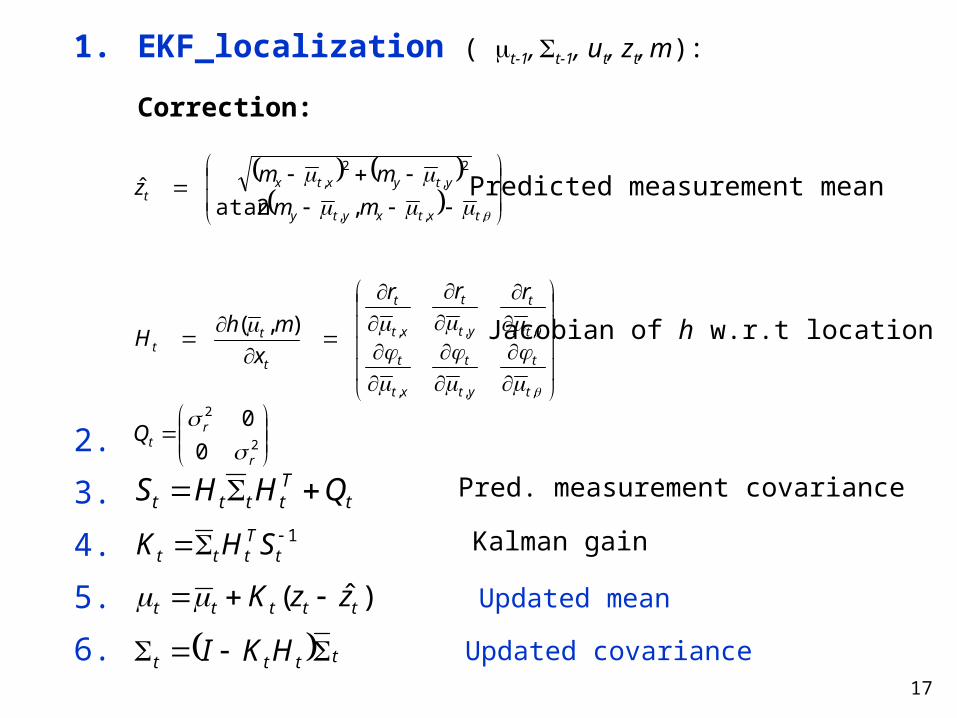
1. EKF_localization ( mt-1, St-1, ut, zt, m):
Correction:
2.
3.
4.
5.
6.
)ˆ( ttttt zzK
tttt HKI SS
,
,
,
,
,
,),(
t
t
t
t
yt
t
yt
t
xt
t
xt
t
t
tt
rrr
x
mhH
,,,
2,
2,
,2atanˆ
txtxyty
ytyxtxt
mm
mmz
tTtttt QHHS S1S t
Tttt SHK
2
2
0
0
r
rtQ
Predicted measurement mean
Pred. measurement covariance
Kalman gain
Updated mean
Updated covariance
Jacobian of h w.r.t location