extended'biomechanical'model'of'the' … carolina... ·...

!!!!!!

Ana!Carolina!Pinto!da!Silveira!!

!!

Extended'Biomechanical'Model'of'the'Ankle4Foot'Complex:'Incorporation'of'

Muscles'and'Ligaments'!

!!!

Thesis&submitted&for&the&degree&of&Master&in&Biomedical&Engineering&

!!!!!!Thesis'Supervisors:'!!!!!!!Prof.!Dr.!Ilse!Jonkers!(Dept.!of!Kinesiology,!KU!Leuven)!!!!!!!!Prof.!Dr.!Maria!Augusta!Neto!(Dept.!of!Mechanical!Engineering,!University!of!Coimbra)!!!!!!!!Dennis!Vandenbussche!(RS!Print,!Paal,!Belgium)!Assessor:'!!!!!!!Prof.!Josef!Vander!Sloten!(Dept.!of!Mechanical!Engineering,!KU!Leuven)'Mentors:'!!!!!!!Wouter!Aerts!(Dept.!of!Mechanical!Engineering,!KU!Leuven)'!!!!!!!Tiago!Malaquias!(Dept.!of!Mechanical!Engineering,!KU!Leuven)!!!!

Coimbra,!2015!!!!!!!

!!!!!!!!!!!!!!!!!!!!!!!!

!!!!!!!!!!!!!!!!!!!!!!!

Master!thesis!developed!in!cooperation!with:!!!!

!!!

!!!

!!!

!! !

!!!!!!!!!!!!!!!!!!!!!!!!!!!!!!!!!!!!!!!!!!!!!!!

!!!!!!!!!!!!!!!!!!!!!!!!!!!!!!!!!!!!!Esta!cópia!da!tese!é!fornecida!na!condição!de!que!quem!a!consulta!reconhece!que!os!direitos! de! autor! são! pertença! do! autor! da! tese! e! que! nenhuma! citação! ou!informação!obtida!a!partir!dela!pode!ser!publicada!sem!a!referência!apropriada.!!This!copy!of!the!thesis!has!been!supplied!on!condition!that!anyone!who!consults!it!is!understood! to! recognize! that! its! copyright! rests! with! its! author! and! that! no!quotation! from! the! thesis! and! no! information! derived! from! it! may! be! published!without!proper!acknowledgement.!!!

Preface

The moment of finishing my master thesis marks the end of the most challengingand fulfilling ride so far. The past five years have been a tremendous experience,that would not be possible if not being surrounded by incredible people.

I want to express my most sincere gratitude to professor Ilse Jonkers. Thank youfor showing me what true guidance, trust and support are. Thank you for integratingme so well in the team, for always caring so much and for making this experience soremarkable. I also want to thank Professor Jos Vander Sloten for the valuable inputgiven to this work and for the wise advices both during last year and this semester.To professor Maria Augusta Neto, for being my supervisor in Coimbra and for theconfidence placed in me.

I must also thank Tristan Kuijpers for introducing me to the Aladyn project,and, of course, to Dennis Vandenbussche for providing me the opportunity to workin such an interesting project.

A huge thank you to Wouter Aerts, for being the best mentor any studentcould ask for. Thank you for all the patience, kindness, willingness to help and forrepeatedly answering my questions. To Tiago Malaquias, for putting so much e↵ortinto this topic and for working side by side with me. Thank you for the motivation,enthusiasm and invaluable contribution. To Tassos Natsakis, for the valuable remarksand readiness to help whenever needed.

I feel very fortunate to have been part of such an exceptional team. I could nothave asked for any better.

I cannot forget to thank professor Isabel Lopes for making possible my participa-tion in both Erasmus and Erasmus+ mobility programs.

A big thank you to my friends in Coimbra and in Leuven, for being my constantinspiration, for reminding me of what is really important in life and for making thisride so wonderful.

Finally, I want to thank my beautiful family, for fully supporting and encouragingmy adventures. For accompanying me, everyday, with no exception, even when livingin a di↵erent country. Thank you for the endless support and for always believing inme.

Ana Carolina Pinto Silveira

i

Contents

Preface i

Abstract v

Resumo vii

List of Figures ix

List of Tables xi

List of Abbreviations and Symbols xiii

1 Introduction 11.1 Defining the Problem . . . . . . . . . . . . . . . . . . . . . . . . . . . 21.2 Objectives and Motivation . . . . . . . . . . . . . . . . . . . . . . . . 31.3 Document Structure . . . . . . . . . . . . . . . . . . . . . . . . . . . 4

2 Literature Study 52.1 Anatomy of the Human Foot . . . . . . . . . . . . . . . . . . . . . . 52.2 The Human Gait Cycle . . . . . . . . . . . . . . . . . . . . . . . . . 172.3 State of the Art: Existing Foot-ankle models . . . . . . . . . . . . . 182.4 Conclusion . . . . . . . . . . . . . . . . . . . . . . . . . . . . . . . . 23

3 Methods 253.1 Model Construction . . . . . . . . . . . . . . . . . . . . . . . . . . . 273.2 Experimental Data Collection . . . . . . . . . . . . . . . . . . . . . . 343.3 Scaling of the Model . . . . . . . . . . . . . . . . . . . . . . . . . . . 353.4 Model Validation . . . . . . . . . . . . . . . . . . . . . . . . . . . . . 373.5 Conclusion . . . . . . . . . . . . . . . . . . . . . . . . . . . . . . . . 43

4 Results 454.1 Kinematics . . . . . . . . . . . . . . . . . . . . . . . . . . . . . . . . 454.2 Dynamics . . . . . . . . . . . . . . . . . . . . . . . . . . . . . . . . . 474.3 Conclusion . . . . . . . . . . . . . . . . . . . . . . . . . . . . . . . . 48

5 Discussion 515.1 Kinematics . . . . . . . . . . . . . . . . . . . . . . . . . . . . . . . . 515.2 Dynamics . . . . . . . . . . . . . . . . . . . . . . . . . . . . . . . . . 53

6 Conclusion 59

A Intrinsic Muscles 63

iii

Contents

B Ligaments 67

C Abstract: CMBBE 2015 73

Bibliography 75

iv

Abstract

Current musculoskeletal foot-ankle models have a limited complexity and thereforethey are not able to capture the full functionality of the foot-ankle complex. However,in the context of the Aladyn project, which aims at developing custom insoles withdynamic structures through 3D printing, there is need to model this complexityfor extending the level of scientific evidenced-based insole design using multi-bodydynamic simulations.

In this work, an extended musculoskeletal foot model is developed in OpenSim,incorporating the foot anatomical structures, intrinsic muscles and ligaments. Afive-segment foot model is developed including a talus, calcaneus, midfoot, forefootand toes segment. Five joints interconnect these segments and connect them with thelower leg segment: ankle (tibia-talus), subtalar (talus-calcaneus), chopart (calcaneus-midfoot), tarsometatarsal (midfoot-forefoot) and metatarsophalangeal (forefoot-toes).Two foot models were constructed with di↵erent number of degrees-of-freedom (DOF):an eight DOF and a fifteen DOF. Based on the number of foot segments spanned,thirty intrinsic muscles and thirty-six ligaments are included. The characteristicparameters of these anatomical structures are retrieved from literature. Experimentalmotion capture data, including marker trajectories, force and plantar pressure dataof five healthy subjects is used to perform the scaling, inverse kinematics and inversedynamics analysis.

Both the kinematic and dynamic results, are very consistent with literature. Theeight DOF model proved to be more suitable to serve the purpose of this project.It presented less inter-subject variability when compared to the fifteen DOF model.The presence of ligaments in the model is found to contribute to the generation ofjoint moment and power. However, further work on the refinement of the parametersthat characterize the intrinsic muscles and ligaments is necessary before proceedingto forward simulation analysis, and as such that it can be used in clinical practice.

v

Resumo

Actualmente, os modelos tridimensionais musculoesqueleticos do complexo pe-tornozelonao sao representativos de toda a funcionalidade e complexidade do pe humano.Neste trabalho, inserido no projeto Aladyn (cujo objetivo e desenvolver palmilhaspersonalisadas com estruturas dinamicas atraves da impressao 3D), ha necessidade decriar um modelo mais representativo desta complexidade para elevar o nıvel cientıficodo design de palmilhas atraves de simulacoes dinamicas de corpos multiplos.

Assim, e desenvolvido um modelo musculoesqueletico do pe-tornozelo em OpenSim,incorporando estruturas anatomicas ao nıvel do pe: musculos intrınsecos e ligamentos.O modelo contem cinco segmentos: calcaneo, talus, medio-pe, ante-pe e dedos. Ossegmentos sao interligados por quatro articulacoes: subtalar (talus - calcaneo), chopart(calcaneo - medio-pe), tarsometatarsal (medio-pe - ante-pe) e metatarsofalangeana(ante-pe - dedos); e por sua vez, estes sao ligados a parte inferior da perna atravesda articulacao do tornozelo (tibia - talus). Tendo em conta o numero de articulacoes,sao construıdos dois modelos com diferentes graus de liberdade: um deles com oitoe o outro com quinze graus de liberdade. De acordo com o numero de segmentosdo pe, sao incluıdos trinta musculos intrınsecos e trinta e seis ligamentos. Dadosexperimentais de captura de movimentos humanos motion capture, forca e pressaoplantar de 5 sujeitos saudaveis sao usados para realizar o dimensionamento do modelo,bem como analises de cinematica inversa e dinamica inversa.

Os resultados obtidos, tanto cinematicos como cineticos estao de acordo coma literatura. O modelo de oito graus de liberdade revela ser mais adequado parao proposito deste projeto, pois apresenta menos variabilidade inter-sujeito quandocomparado com o modelo de 15 graus de liberdade. A incorporacao de ligamentos nomodelo demonstra contribuir para a geracao de momento e energia, principalmenteao nıvel das articulacoes do medio-pe e ante-pe. E necessario trabalho futuro nosentido de ajustar os parametros que caracterizam os musculos e os ligamentos,antes de se avancar para aplicacoes em dinamica direta, tal que o modelo possa serutilizado em praticas clınicas.

vii

List of Figures

2.1 Reference planes with respect to human anatomy. . . . . . . . . . . . . . 62.2 Bones of the foot, dorsal and plantar view. . . . . . . . . . . . . . . . . 72.3 Schematic representation of the foot axis defined by Hicks [11]. . . . . . 92.4 The dorsal and plantar views of the intrinsic muscles of the foot. . . . . 132.5 Origin and insertion points of the intrinsic muscles of the foot: dorsal

and plantar view. . . . . . . . . . . . . . . . . . . . . . . . . . . . . . . . 142.6 Ligaments and tendons of the ankle-foot complex: medial and lateral view. 152.7 The human gait cycle for the right foot. . . . . . . . . . . . . . . . . . . 172.8 Detail of the stance and swing phase of the gait cycle. . . . . . . . . . . 182.9 Eight segments of the human foot model proposed by Scott and Winter

[29]. . . . . . . . . . . . . . . . . . . . . . . . . . . . . . . . . . . . . . . 212.10 Musculotendon actuator model used in the work of Delp [32]. . . . . . . 22

3.1 Project workflow. . . . . . . . . . . . . . . . . . . . . . . . . . . . . . . . 253.2 The joints and DOF of the 3-segment OpenSim gait model

(3DGaitModel2392). . . . . . . . . . . . . . . . . . . . . . . . . . . . . . 263.3 Foot extrinsic muscles of the OpenSim gait model (3DGaitModel2392),

right foot. . . . . . . . . . . . . . . . . . . . . . . . . . . . . . . . . . . . 263.4 The five segments of the extended foot model. . . . . . . . . . . . . . . . 273.5 The 15 DOF of the 5-segment model. . . . . . . . . . . . . . . . . . . . 283.6 Foot intrinsic muscles incorporated in the extended OpenSim model. . . 303.7 Ligament characteristic force-displacement curve. . . . . . . . . . . . . . 323.8 Ligaments incorporated in the extended foot model: medial and lateral

view. . . . . . . . . . . . . . . . . . . . . . . . . . . . . . . . . . . . . . . 323.9 Ligaments incorporated in the extended foot model: plantar and dorsal

view. . . . . . . . . . . . . . . . . . . . . . . . . . . . . . . . . . . . . . . 333.10 Location of the foot markers: right foot. . . . . . . . . . . . . . . . . . . 353.11 Example of the distance between one pair of experimental markers and

one pair of model markers. . . . . . . . . . . . . . . . . . . . . . . . . . 363.12 Graphical representation of the linear marker weight attribution for the

di↵erent cases. . . . . . . . . . . . . . . . . . . . . . . . . . . . . . . . . 393.13 Example of the inter-marker distance for one trial and the respective

marker weight attribution . . . . . . . . . . . . . . . . . . . . . . . . . . 403.14 Example of plantar pressure map and segment division for one trial . . 42

ix

List of Figures

3.15 Vertical component of the external loads acting on the foot segments. . 423.16 Example of the vertical force component of the ground reaction forces

acting on the four segments in contact with the ground, for one trial. . . 43

4.1 Kinematic results of the 8 DOF and 15 DOF model . . . . . . . . . . . 464.2 Ankle moment and power obtained in the work of Burg [20] . . . . . . . 484.3 Joint moments of the 8 DOF model. . . . . . . . . . . . . . . . . . . . . 494.4 Joint powers of the 8 DOF model. . . . . . . . . . . . . . . . . . . . . . 50

5.1 Ligaments of the ankle and subtalar joint incorporated in OpenSim. . . 545.2 Joint moment for the 3 DOF of the ankle joint of the 15 DOF model. . 555.3 Joint power for the 3 DOF of the ankle joint of the 15 DOF model. . . . 555.4 Example of the force-length curve of the plantar fascia. . . . . . . . . . 565.5 Example of the results of the inverse dynamics for the tarsometatarsal

first ray joint and for the metatarsophalangeal plantarflexion/dorsiflexionjoint. . . . . . . . . . . . . . . . . . . . . . . . . . . . . . . . . . . . . . . 57

x

List of Tables

A.1 Parameters of the foot intrinsic muscles. . . . . . . . . . . . . . . . . . . 63A.2 Geometry path of the intrinsic muscles - part 1. . . . . . . . . . . . . . . 64A.3 Geometry path of the intrinsic muscles - part 2. . . . . . . . . . . . . . . 65A.4 Geometry path of the intrinsic muscles - part 3. . . . . . . . . . . . . . . 66

B.1 Parameters of the foot ligaments. . . . . . . . . . . . . . . . . . . . . . . 68B.2 Ligaments’ geometry path - part 1 . . . . . . . . . . . . . . . . . . . . . 69B.3 Ligaments’ geometry path - part 2 . . . . . . . . . . . . . . . . . . . . . 70B.4 Ligaments’ geometry path - part 3 . . . . . . . . . . . . . . . . . . . . . 71B.5 Ligaments’ geometry path - part 4 . . . . . . . . . . . . . . . . . . . . . 72

xi

List of Abbreviations andSymbols

Abbreviations

AB Abduction

ABDH Abductor Hallucis

ABDM Abductor Digiti Minimi

AD Adduction

ADHO Adductor Hallucis Oblique

ADHT Adductor Hallucis Transverse

a.-p.m.-t.

Anterior-posterior mid-tarsal axis

CT Computer Tomography

d.a. Dorsiflexion axis

DI Dorsal Interosseous

DF Dorsiflexion

DOF Degrees of Freedom

EDB Extensor Digitorum Brevis

EHB Extensor Hallucis Brevis

EV Eversion

FDB Flexor Digitorum Brevis

FDMB Flexor Digiti Minimi Brevis

FHB Flexor Hallucis Brevis

FHBL Flexor Hallucis Brevis Lateralis

FHBM Flexor Hallucis Brevis Medialis

IC Initial Contact

IMD Inter-Marker Distance

IV Inversion

LB Lumbricals

MoCap Motion Capture

o.m.-t. oblique mid-tarsal axis

p.a. plantarflexion ankle axis

xiii

List of Abbreviations and Symbols

PCSA Physiological Cross-Sectional Area

PF Plantarflexion

PI Plantar Interosseous

QPL Quadratus Plantar Lateralis

QPM Quadratus Plantar Medialis

SD Standard Deviation

t.c.n. Talo-calcaneo-navicular axis

TO Toe O↵

XML Extensible Markup Language

1r. Fist ray axis

5r. Fifth ray axis

Symbols

C(q, q) Vector of Coriolis and centrifugal forces

F Force

G(q) Vector of gravitational forces

k Sti↵ness

L0 Ligament resting length

L Ligament length

M Moment of force

M(q) System matrix

P Power

q Vector of generalized positions

q Vector of generalized velocities

q Vector of generalized accelerations

" Strain

⌧ Vector of generalized forces

! Angular velocity

xiv

Chapter 1

Introduction

Gait is the most common of human movements. Even though it is usually takenfor granted, it is one of the most complex and totally integrated movements. It hasbeen described and analysed more than any other movement. In fact, understandingthe actual patterns of movement of humans and animals goes back to prehistorictimes [1]. In 1836 the Weber brothers made one of the first mechanical analysisof human locomotion, describing the phases of human walking as well the motionof the centre of mass. They also analysed disorders of the gait pattern [2]. Theappearance of photographic and motion picture cameras contributed to revolutionizethe study of the human movement, revealing details that were not possible tovisualize before. In 1887 Muybridge presented sequential photography techniquesto analyse human gait [3], [2]. In the 19th century it was possible to perform thevery first recordings of human locomotion patterns [1]. Nowadays it is possible toconduct even more precise experiments due to: the development of more accuratemotion capture systems, which make use of video, infra-red cameras and laser oracoustic emission systems (e.g. Vicon r, Oxford Metrics, UK); the use of force platesand plantar pressure measurement systems; furthermore, advances in the computersimulation field allowed estimating dynamic variables that cannot be directly observedor measured, for instance, the muscle forces or the trajectory of the bodies’ centreof mass, moments of force, mechanical energy, etc. Consequently, musculoskeletalmodels, in which the human body is divided and modelled in segments that areinterconnected by joints, have become a popular tool to study human gait as well asto calculate muscle forces in combination with dynamic simulations of motion, sincethey make use of inverse solutions to estimate or calculate these dynamic variables[2]. Thus, biomechanical modelling techniques can be used as a diagnostic, surgeryplanning or rehabilitation tool that can guide clinical decision making, or simplyincrease the quality of life of healthy subjects by providing more suitable footwear.This is possible thanks to the simulation and prediction tools, allowing to reveal, forinstance, how much muscle strength is required to do a certain movement, or theforces and moments that a musculoskeletal system produces during a specific motion,or even to understand how changing the insertion point of a tendon can a↵ect itsmoment curve profile.

1

1. Introduction

However, in the current musculoskeletal models, the level of detail included todescribe foot biomechanics is limited. Nevertheless, biomechanical modelling of thefoot can, among others, actively contribute to: study gait disorders and pathologiesrelated to the foot, improve athletic performance or design subject-specific customizedinsoles.

Therefore, this master thesis aims to develop an extended musculoskeletal modelof the human foot in OpenSim, a freely available, user extensible software that allowsthe development of musculoskeletal models and dynamic simulations of movement[4].

1.1 Defining the Problem

The foot provides support to the human body by distributing gravitational andinertial loads [5]. Despite playing a fundamental role in human gait, there is still muchto unveil before it is possible to fully understand its intrinsic kinematics and dynamics.It is a structurally complicated unit and its basic load-carrying mechanisms remaina vivid subject of debate in the biomechanics community [6]. So far, an unbiasedunderstanding of the foot kinematics has been di�cult to achieve due to, precisely,the complexity of the foot structure and motion [6]. This complexity arises from thenumber of small bones, muscles and ligaments that the foot is able to comprise. Dueto this elaborateness, biomechanical models often treat the foot as a rigid segment,with no relative movement between the functional units or segments within the foot[7], [8]. Consequently, these models do not provide a realistic representation of thefoot structure and its kinematics. As a result, the multi-segmental and deformableproperties of the foot are not taken into account. While the use of these simplemodels might be reasonable to quantify ankle moments and powers during gait usinginverse dynamics analysis [9], it is not advisable for performing contact simulationanalysis or for modelling the e↵ect of foot insoles on the movement of the footstructure. Furthermore, in many foot disorders (for example, flat feet, midfoot break,overpronation, etc.), these simple models do not allow a valid representation of thespecific dysfunction that is often related to pathological movement between individualfoot segments. In these cases, a realistic representation of the foot structure and itskinematics is required.

Multi-segment kinematic foot-ankle models, have been defined to capture footkinematics and quantify it in health and disease [10]. They simplify the complexanatomical structure of the foot by grouping several neighbour bones together,creating the so called foot segments. The segments then act as rigid bodies, meaningthat there is no movement within the segment. These kinematic models are primarilyused for clinical gait analysis purposes, quantifying the joint angles and moments.They di↵er from musculoskeletal models as muscles are not included in kinematicmodels. As such, the aim of kinematic models is to analyse and document inter-segment motion.

For simulation purposes, the current musculoskeletal models should not onlyincorporate a similar multi-segment definition as the kinematics models. In addition,

2

1.2. Objectives and Motivation

the characteristic parameters of the foot muscles and ligaments, such as the ligamentslack length, the muscle physiological cross sectional area or force, need to be defined.This specific information is currently only limited available as there are only veryfew studies concentrating on experimentally documenting these specific parameters.

In conclusion, the state of the art for musculoskeletal models of the foot-anklecomplex for use in dynamic simulations of gait are highly simplified and do notaccount for the complex ligamentous and muscle control of the foot-ankle kinematics.The development of a detailed foot-ankle model is a pre-requisite to increase the un-derstanding of foot pathologies and the design of adequate therapeutic interventions.

1.2 Objectives and Motivation

This master thesis is developed in the context of the Aladyn project, a joint collabo-ration between three industrial partners, Materialise NV, RS Scan and RS Print, andthe KU Leuven as the research partner. The goal is to produce custom insoles withdynamic structures through 3D-printing. In order to do this, it is necessary to havea more scientific evidence-based insole design approach, since until now this processis mainly based on subjective decision making by the orthotic technicians, without aconsistent and solid base. Thus, the Aladyn project aims at creating a fully auto-mated digital workflow from patient assessment to the production of subject-specificinsoles based on objective evidence. There are three distinctive knowledge domainsidentified in this project: biomechanical patient assessment, evidence-based insoledesign through modelling and 3D-printing of insoles with dynamic structures. Thisthesis work falls into the second knowledge domain.

Therefore, the primary purpose of this master thesis is to define and validate anextended foot-ankle musculoskeletal model in OpenSim. The specific objectives are:

• Increasing the level of detail of the current OpenSim foot model, by extendingthe anatomical and functional detail of the foot structures: firstly, the numberof foot segments and the degrees-of-freedom (DOF) between them need tobe increased to represent physiological foot function. This goal must beaccomplished based on a literature study documenting in detail the foot-anklekinematics and the associated joint axes. Secondly, the most relevant intrinsicmuscles and ligaments of the foot that control the included segments need to beincorporated. This goal must be accomplished by investigating and gatheringthe respective muscle/ ligament parameters and geometry information fromliterature. The model definition will be implemented according to the OpenSimmodel formulation.

• Validation of the performance of two foot-ankle models, one with 8 DOF andthe other with 15 DOF. This relies on inverse kinematics analysis using a dataset of 3D integrated motion capture (MoCap) that included a multi-segmentfoot definition. Calculated kinematics are compared against a golden standardof foot-ankle kinematics obtained through bone anchored pins.

3

1. Introduction

• Evaluation of the ligament forces by performing inverse dynamics analysis.Ranges of ligament forces are evaluated only qualitatively, as no golden standardis available in literature.

The expected outcome of this work is the development of an extended muscu-loskeletal foot model, that can be used, in combination with 3D motion captureand dynamic motion simulations, as a decisive tool in the making of customized3D-printed insoles.

1.3 Document Structure

The second chapter of this thesis consists of the literature study. It starts by presentingthe anatomy of the human foot, followed by the human gait cycle. The last sectionof the chapter focus on reviewing the already existing solutions regarding kinematic,kinetic and musculoskeletal models. Chapter 3 consists of the methods used toextend and validate the developed foot model. It defines the model constructionprocedure, as well as the scaling and validation. The fourth chapter presents theresults obtained in terms of kinematics and dynamics. Chapter 5 discusses the resultsobtained as well as the challenges faced during the course of this work. At the end ofeach chapter a brief conclusion is presented, except for chapter 5, since its conclusionis part of the final chapter. Finally, in the last chapter, a conclusion is formulatedand future work is defined.

Three appendices are included in this work. Appendixes A and B present theinput parameters to model the intrinsic muscles and ligaments. Finally, appendix Cincludes the abstract of the publication to be presented in the thirteenth InternationalSymposium on Computer Methods in Biomechanics and Biomedical Engineering2015 (CMBBE), by the KU Leuven Ankle-Foot group.

4

Chapter 2

Literature Study

The aim of the present chapter is to address the anatomy of the foot in terms of itsbones, joints, intrinsic muscles and ligaments, providing an overview of the importantanatomical structures that need to be added to the extended musculoskeletal model ofthe foot. Secondly, the di↵erent phases of the human gait cycle are briefly explained.Finally, a literature review of the already existing kinematic and dynamic foot modelsis presented and a brief conclusion is formulated.

It is necessary to first establish the terminology used in this work in terms of theanatomical reference system, as a variety of terms that describe the 3-dimensionalmovement of the foot are found in literature. Figure 2.1 shows the reference planeswith respect to the human anatomy. The sagittal plane divides de body into a rightand a left part; the frontal, also known as coronal plane, divides the body into ananterior and a posterior part; and the transverse or horizontal plane is perpendicularto the sagittal and frontal planes. Therefore, the vertical axis is the Y axis, theanterior-posterior direction is the X axis and the medial-lateral direction is the Zaxis, figure 2.1. Furthermore, the terminology used in this work to describe the 3Dmovement of the foot is as follows: dorsiflexion/plantarflexion or extension/flexioncorrespond to rotation about a medial-lateral axis; abduction/adduction, to rotationabout a vertical axis; and inversion/eversion to rotation about an anterior-posterioraxis. It is also important to note that some authors, such as Hicks [11], referto the rotation about an anterior-posterior axis as supination/pronation whilstin this work this rotation is referred to as inversion/eversion. The terminologysupination/pronation is used in this work to describe a combined movement ofinversion/eversion in the frontal plane, adduction/abduction in the transverse planeand plantarflexion/dorsiflexion in the sagittal plane, respectively.

2.1 Anatomy of the Human Foot

The human foot is considered to be a very complex and intricate structure due tothe number of elements and joints it comprises despite its relatively small size. It is,therefore, essential to understand the basics of the foot anatomy in terms of bones,joints, muscles and ligaments, as well as understanding the interaction between these

5

2. Literature Study

Figure 2.1: Reference planes with respect to human anatomy. Figure adapted from[12]

structures in order to build a biomechanical foot model. Regardless of what researchdefines as the human gait cycle and the role of the foot, the one constant remainsanatomy [13], being of paramount importance to understand it before anything else.

2.1.1 Foot Bones

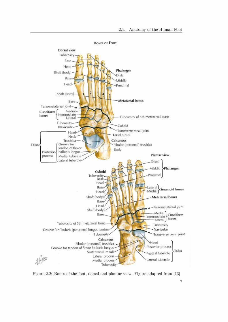
The foot includes twenty-six bones: seven tarsals, five metatarsals and fourteenphalanges, figure 2.2. The tarsals are the talus, calcaneus, navicular, three cuneiforms(medial, intermediate and lateral) and the cuboid. The arrangement and relativepositioning of the bones imposes a limited independence between them [13].

The talus plays the critical role of connecting the lower leg to the foot sinceit articulates with the tibia and fibula, which are the lower leg bones, and it alsoarticulates with the calcaneus and navicular. The calcaneus is the largest bone ofthe foot and is commonly referred to as the heel bone. It contains three articularsurfaces (the posterior, middle, and anterior facets) allowing the talus to articulatewith it, forming the subtalar joint. The navicular is located between the head of thetalus and the three cuneiforms and it has a flattened oval shape. It connects withthe talus through the talonavicular joint. The three cuneiforms are all wedge shapedand line up side by side in the midfoot, with the broader side of the wedge oriented

6

2.1. Anatomy of the Human Foot

Figure 2.2: Bones of the foot, dorsal and plantar view. Figure adapted from [13]

7

2. Literature Study

plantarly on the medial cuneiform and dorsally on the intermediate and lateralcuneiforms. They articulate with the navicular forming the naviculocuneiform joint.The cuboid is a square-shaped bone on the lateral side of the foot interposed betweenthe calcaneus and the fourth and fifth metatarsals. The main joint formed with thecuboid is the calcaneocuboid joint. The metatarsals are long bones, relatively flatdorsally and concave longitudinally on the plantar sides. They are each composed ofa base, a body and a head and are numbered from one (medial) to five (lateral). Thebases of the second and third metatarsals articulate with the cuneiforms and the baseof the fifth with the cuboid, creating the Lisfranc joint (or the tarsaometatarsal joint).The heads articulate with the proximal phalanges, forming the metatarsophalangealjoint. The first metatarsal is the broadest and most massive of the five. It has abroad head and its plantar surface has two grooves where the sesamoids lie withinthe tendons of the flexor hallucis brevis muscle. Finally, the phalanges are the bonesof the toes. They are short and are divided into proximal, middle and distal. Eachtoe has three bones except for the great toe which has two [13].

2.1.2 Foot Joints

A joint is defined as the place where two bones connect or articulate. In termsof joint function, there are three di↵erent joint classes: the synarthroses, whichare immovable since the surfaces of the bones are in almost direct contact; theamphiarthroses, which are slightly movable, being the surface of the bones connectedby ligaments or cartilage; and the synovial joints or diarthroses, which are the mostcommon in the human body. The latter are characterized as freely movable joints,in which there is space between the adjoining articular surfaces and the space islubricated by synovial fluid. The synovial joints are the most relevant as all thejoints studied in this work are of the synovial type. These joints can be classifiedin several types according to the kind of motion permitted in each of them. Thefollowing synovial joints are present in the foot: the Hinge joint, where motion isonly possible in one plane, for example, the interphalangeal joint; the Gliding joint,also known as planar joint, admits a gliding movement in any direction along theplane of the joint, it can be found between bones that have flat articular surfaces,being the tarsometatarsal joint an example; and the Condyloid joint, in which flexion,extension, adduction, abduction and circumduction are possible and it is present, forexample, in the metatarsophalangeal joint [14].

Ankle Joint

The ankle joint is the articulation between the tibia and the talus and it is agreed tobe a synovial joint of the hinge type, also known as tibiotalar joint. The synovialmembrane of the ankle joint has the capacity to extend upwards, causing largeamount of synovial liquid to concentrate there [13]. The primary movement of thisjoint is dorsiflexion (extension) and plantarflexion (flexion), however just like in mostof the foot joints, there is a combination of other minimal movements happening atthe joint as opposed to a unique and simply defined movement. As described by

8


Figure 2.3: Schematic representation of the foot axis defined by Hicks [11]: theplantarflexion ankle axis (p.a.), dorsiflexion ankle axis (d.a.), talo-calcaneo-navicularaxis (t.c.n.), oblique mid-tarsal axis (o.m.-t.), anterior-posterior mid-tarsal axis (a.-p.m.-t.), first ray axis (1r.) and fifth ray axis (5r.). Figure adapted from [11]

Hicks [11] and in agreement with the work of Barnett and Napier [15], a dorsiflexionankle axis (d.a.) and plantarflexion ankle axis (p.a.) were defined at the ankle level,2.3. These axis are oblique in both the sagital and transverse planes, therefore, theminor and minimal movements that accompany flexion-extension at the ankle areabduction/adduction and inversion/eversion [16].

Subtalar and Talocalcaneonavicular joints

The subtalar joint is one of the six intertarsal joints, being the other five the talocal-caneonavicular, calcaneocuboid, transverse tarsal, cuneonavicular and intercuneiform.It is the joint between the underside of the body of the talus and the posterior surfaceof the superior aspect of the calcaneus. There is a loose, thin-walled articular capsuleuniting the bones in the margins of the articular surfaces [13].

The talocalcaneonavicular joint is composed of two joints that function as a unit:the posterior talocalcaneal joint and the anterior talocalcaneal joint. The axis of this

9

2. Literature Study

joint, according to [11] is oblique, oriented upward, anteriorly and medially and has atransverse, vertical and longitudinal component. Each component generates motion,hence, this joint produces a combination of three motions: eversion-abduction-extension or inversion-adduction-flexion.

Chopart Joint

The transverse tarsal joint, also known as Chopart joint, crosses the foot from sideto side, consisting of the talonavicular and the calcaneocuboid joints [13]. Thetalonavicular joint is an integral part of the talocalcaneonavicular complex and movesalong with the subtalar joint but it can also move in unison with the calcaneocuboidjoint, independently of the subtalar. Thus, the navicular rotates with respect to thetalus about three di↵erent axis depending on which complex it is moving along with,but always acts as a hinge joint. The calcanocuboid is a saddle joint [16].

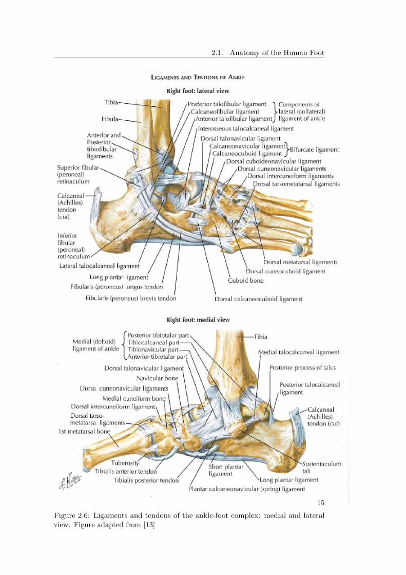
As presented in figure 2.3, and according to Hicks [11] there are two axis that definethe Chopart joint: the oblique mid-tarsal axis (o.m.-t.) and the anterior-posteriormid-tarsal axis (a.-p. m.-t.). The movement allowed in the first one is eversion-abduction-extension or inversion-adduction-flexion and in the latter eversion withslight abduction-extension or inversion with slight adduction-flexion. In conclusion,these joints contribute mainly to the inversion/ eversion of the foot.

Tarsometatarsal Joint

The tarsometatarsal, also known as Lisfranc’s joint, is composed of plane jointsbetween the medial three metatarsals bases with the cuneiforms, and the two lateralmetatarsals bases with the cuboid. It allows flexion/extension of the metatarsalrays and some longitudinal axial rotation-inversion and rotation-eversion at themarginal rays [16]. Observing figure 2.3, it is possible to identify two axes at thetarsometatarsal joint: the 1st ray axis (1 r.) and the 5th ray axis (5 r.). Both axesallow for flexion-eversion or extension-inversion [11].

Metatarsophalangeal Joint

These joints are condyloid joints between the heads of the metatarsals and theextremities of the proximal phalanges. As such, dorsiflexion, plantarflexion, abduction,adduction and circumduction are the movements at these joints. However, the primarymovement is, undoubtedly, dorsiflexion/plantarflexion. Each joint is enclosed by anarticular capsule and reinforced by plantar and collateral ligaments [13].

2.1.3 Intrinsic Muscles

The muscles are the structures that allow bone movements through its contractileforces. As agglomerates of fibers, they are responsible for creating movement inthe human body. The sarcomere is the functional unit of the muscles, and it iscomposed of contractile proteins or filaments which are the responsible for the musclecontraction. A muscle contracts when it is activated and this activation is controlled

10


by the somatic nervous system, which triggers an action potential. When contracting,the muscles develop force and create a torque about one or more joints spanned bythose muscles. Nevertheless, muscles are able to accelerate bodies that they do notspan due to a phenomenon denominated dynamic coupling, in which a force appliedby each muscle is transmitted through the bones of the skeleton to all the joints [17].

The tendons, which are strong fibrous collagen tissue, attach the muscles to thebones of the skeleton. At the foot, extrinsic and intrinsic muscles are discriminated.The foot extrinsic muscles originate in the femur, tibia or fibula and insert on oneof the foot bones, while the intrinsic muscles have both their origin and insertionpoints in the foot.

The intrinsic muscles of the foot are twenty-eight and are located both in theplantar and the dorsal aspects of the foot. It is widely accepted [13] [16] that theplantar foot can be divided in four relevant compartments: medial, lateral, centraland interosseous.

The medial compartment comprises the abductor hallucis (ABDH) and flexorhallucis brevis (FHB) muscles as well as the tendon of the flexor hallucis longus(the last one is not considered an intrinsic muscle). The flexor hallucis brevis is atwo-bellied muscle, divided into a medial and lateral component and it allows for theflexion of the hallux through the metatarsophalangeal joint. The abductor hallucismuscle, arising from the calcaneus and inserting into the base of the proximal phalanxof the big toe is the responsible for abduction of the great toe from the axis of thesecond ray.

The lateral compartment consists of the flexor digiti minimi brevis (FDMB)and abductor digiti minimi (ABDM). The first flexes the fifth toe through themetatarsophalangeal joint and the latter abducts the fifth toe from the axis of thesecond ray.

The central compartment contains the flexor digitorum brevis muscles (FDB),the tendon of the flexor hallucis longus and lumbricals (LB), the adductor hallucisand the quadratus plantae muscles. The flexor digitorum brevis muscles dividesinto four tendons and each one of them is then divided, in the proximal phalanges,into two splits that insert in the middle phalanges, figure 2.4. Thus, these musclesare responsible for flexion of the middle phalanges of the lateral four toes and alsocontribute to the metatarsophalangeal flexion of these toes. The quadratus plantaris divided into a medial and a lateral component (QPM and QPL) that merge toform a flattened muscular band. This muscle assists the flexor digitorum longusin flexing the toes. The lumbricals are four small cylindrical muscles that arisefrom the four tendons of the flexor digitorum longus and these muscles flex theproximal phalanges (at the metatarsophalangeal joint) and extend the middle anddistal phalanges. The last muscles of the central compartment are the transverse andthe oblique adductor hallucis (ADHT and ADHO). These muscles adduct the greattoe and play an important role in maintaining the transverse arch of the foot [13].

Finally, the interosseous compartment comprises the plantar interosseous (PI)and the dorsal interosseous (DI). The first are adductors of the third, fourth and fifthdigits while the second are abductors of the digits. Both of the interosseous serve inflexion of the metatarsophalangeal joints [13]. Figure 2.5 illustrates the origin and

11

2. Literature Study

insertion points of the intrinsic muscles of the foot.Regarding the dorsal aspect of the foot, it includes the extensor hallucis brevis

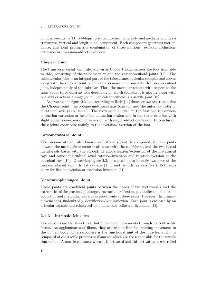
(EHB) and three extensor digitorum brevis muscles (EDB). Figure 2.4 shows theintrinsic muscles of the foot. The extensor digitorum brevis is a broad but thinmuscle that divides into four tendons for the most medial four toes. However, themost medial tendon, which is the largest of the four, is often designated as extensorhallucis brevis muscle [13] [18], as it is possible to observe in figure 2.4. The otherthree tendons merge with the tendons of the extensor digitorum longus (which is notan intrinsic muscle) in the second, third and forth toes, assisting in the extension ofthe proximal phalanges [13].

2.1.4 Ligaments

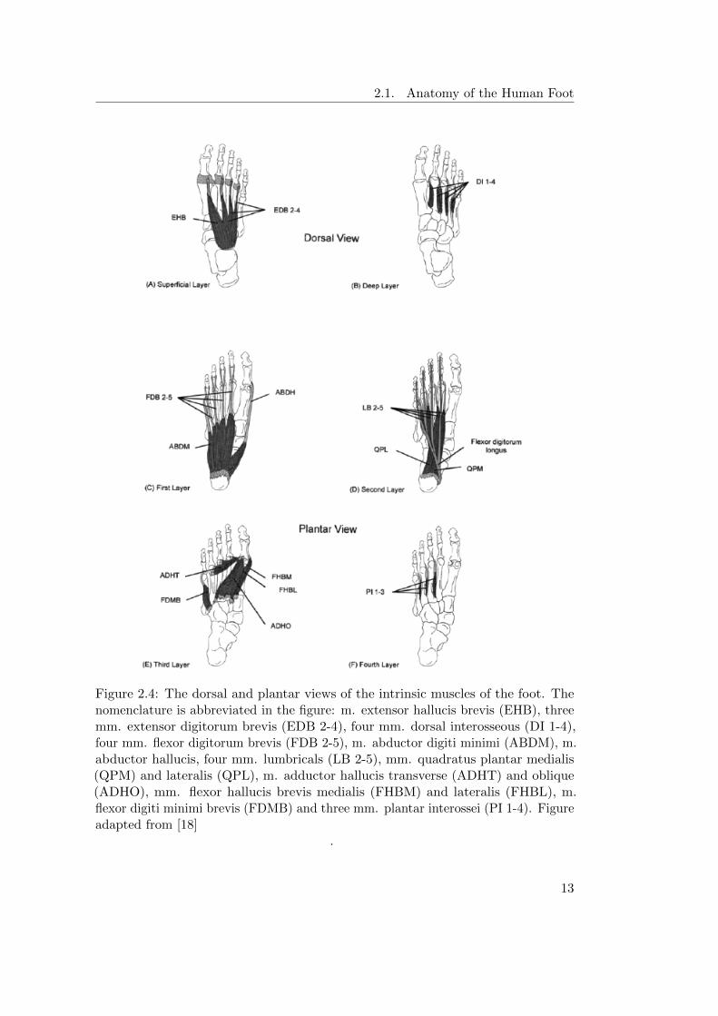
Ligaments are strong structures that attach bones to other bones. They are composedof flexible, fibrous connective tissue and are responsible for stabilizing the joints.Even though they are flexible, they are also rather sti↵ structures in which smalllength changes can cause large passive forces. A brief overview of the ankle-footligaments that are the most relevant to this work is presented. Figure 2.6 illustratesthe ligaments of the ankle-foot complex.

Ankle Ligaments

The ligaments responsible for stabilizing the ankle joint can be divided into threegroups depending on their anatomical location: the lateral ligaments, the deltoidligaments on the medial side, and the ligaments of the tibiofibular syndemosis [19].The first two groups are composed of notably strong ligaments.

The lateral collateral ligament complex consists of the anterior talofibular, thecalcaneofibular and the posterior talofibular ligaments. Firstly, the anterior talofibularligament limits the anterior displacement of the talus and plantarflexion of the ankle.It is virtually horizontal to the ankle in neutral position but inclines upward indorsiflexion and downward in plantarflexion. Only in plantarflexion the ligamentcomes under strain. Secondly, the calcaneofibular is the only ligament bridging boththe talocrural and subtalar joint. It allows flexion/extension of the talocrural jointand also permits subtalar movement depending on its bi-articular characteristics. Thecalcaneofibular becomes horizontal during plantarflexion and vertical in dorsal flexion,remaining tensed throughout the entire arc of motion of the ankle and is relaxedwhile everted and tense during inversion. Thirdly, the posterior talofibular ligamentis relaxed in plantarflexion and in neutral ankle position, while in dorsiflexion it istensed. Since it is a multifascicular ligament, it does not insert in a specific uniqueplace and some of its fibers contribute to form the tunnel for the flexor hallucislongus tendon while other fibers fuse with the posterior intermalleolar ligament [19],[16].

The medial collateral ligament, also known as the deltoid ligament, is a strongand triangular multifascicular group of ligaments and can be divided into a superficialand deep group of fibers. It originates from the medial malleolus to insert in the talus,

12


Figure 2.4: The dorsal and plantar views of the intrinsic muscles of the foot. Thenomenclature is abbreviated in the figure: m. extensor hallucis brevis (EHB), threemm. extensor digitorum brevis (EDB 2-4), four mm. dorsal interosseous (DI 1-4),four mm. flexor digitorum brevis (FDB 2-5), m. abductor digiti minimi (ABDM), m.abductor hallucis, four mm. lumbricals (LB 2-5), mm. quadratus plantar medialis(QPM) and lateralis (QPL), m. adductor hallucis transverse (ADHT) and oblique(ADHO), mm. flexor hallucis brevis medialis (FHBM) and lateralis (FHBL), m.flexor digiti minimi brevis (FDMB) and three mm. plantar interossei (PI 1-4). Figureadapted from [18]

.

13

2. Literature Study

Figure 2.5: Origin and insertion points of the intrinsic muscles of the foot: dorsaland plantar view. Figure adapted from [13]

calcaneus and navicular. Even though there is not much agreement in literature,the most commonly accepted description of this ligament is that it comprises sixbands: three that are always present, the tibiospring, the tibionavicular and the deepposterior tibiotalar ligament, which is the thickest [13] and strongest component ofthe entire medial ligament [16]; and the other three that can vary, the superficialposterior tibiotalar ligament, tibiocalcaneal ligament and deep anterior tibiotalarligament [19].

The tibiofibular syndesmotic ligament complex ensures the stability of the tibiaand fibula and resists the axial, rotational and translational forces that attempt toseparate them. The three ligaments responsible for this are the anterior tibiofibular,the posterior tibiofibular and the interosseous tibiofibular ligament.

Talocalcaneonavicular Ligaments

The talocalcaneonavicular complex comprises the inferior, lateral, posterior, medial,superomedial and interosseous calcaneonavicular ligaments. The inferior calcaneon-avicular ligament, also known as the spring ligament due to its elasticity, is veryfasciculated consisting of a thick bundle of fibers, being the lateral bundle (thatinserts on the beak of the navicular), the strongest. The lateral calcaneonavicular

14


Figure 2.6: Ligaments and tendons of the ankle-foot complex: medial and lateralview. Figure adapted from [13]

15

2. Literature Study

is part of the bifucarte ligament, which is disposed in the form of a V forming anaverage angle of 30 degrees between the two components. The other componentof the bifurcate ligament is the medial calcaneocuboid and it is usually the leaststrong component of the V-shaped ligament. Besides the ones mentioned above, thetalocalcaneonavicular joint also includes the cervical ligament (it is a part of theinterosseous ligament and is also called anterior talocalcaneal ligament) which isthe strongest ligament connecting the talus and the calcaneus. Finally, there is thetalonavicular ligament, which has a superficial and a deep component, being the firsta thin, long band and the second a shorter but deeper band [16].

Hindfoot-Midfoot Ligaments

There are numerous ligaments connecting the hindfoot bones to those of the midfoot,as well as interconnecting the tarsal bones. At the calcaneocuboid joint, three liga-ments are identified: the medial, dorsolateral and inferior calcaneocuboid ligaments.The medial ligament is the outer component of the bifurcate ligament, as mentionedabove. The inferior calcaneocuboid is a thick, powerful plantar ligament with a deepand a superficial component: the short plantar and the long plantar ligaments.

Each of the three cuneiform bones is united to the navicular by both a dorsaland a plantar ligament. The cubonavicular, the dorsal cuneonavicular and thecuneo-cuboid ligaments each have three types: a dorsal, plantar and a interosseous.

Lastly, there are two dorsal, two interosseous and one plantar intercuneiformligaments to keep these three bones together. The dorsal are small rectangular bands,the plantar is a short ligament, while the interosseous is a strong thick transverseligament [16].

Tarsometatarsal Ligaments

The tarsometatarsal joint is very complex one and is secured by seven dorsal ligaments,by a variable number of plantar ligaments and by three sets of interosseous ligaments.The dorsal ligaments guarantee the connection between the bases of the first threemetatarsal rays and the three cuneiforms and between the fifth metatarsal and thecuboid. Even though the plantar cuneometatarsal ligaments are always present,its number and location vary from subject to subject. These ligaments are, ingeneral, stronger than the dorsal ones. The interosseous ligaments are located in theinterspace between the three first metatarsals and the cuneiforms, being the firstone the strongest of the three (also known as the Lisfranc ligament). Finally, thereare the intermetatarsal ligaments in between the metatarsals, and they can also becharacterized in dorsal, plantar and interosseous. It is noteworthy to mention thatthere is no dorsal or plantar ligaments between the first and second metatarsals [16].

Metatarsophalangeal

In the metatarsophalangeal joint, the proximal phalanx and the fibrocartilaginousplantar plate constitute both an anatomical and functional unit. It is at the plantarplate that the two longitudinal septae of the plantar aponeurosis insert as well as

16

2.2. The Human Gait Cycle

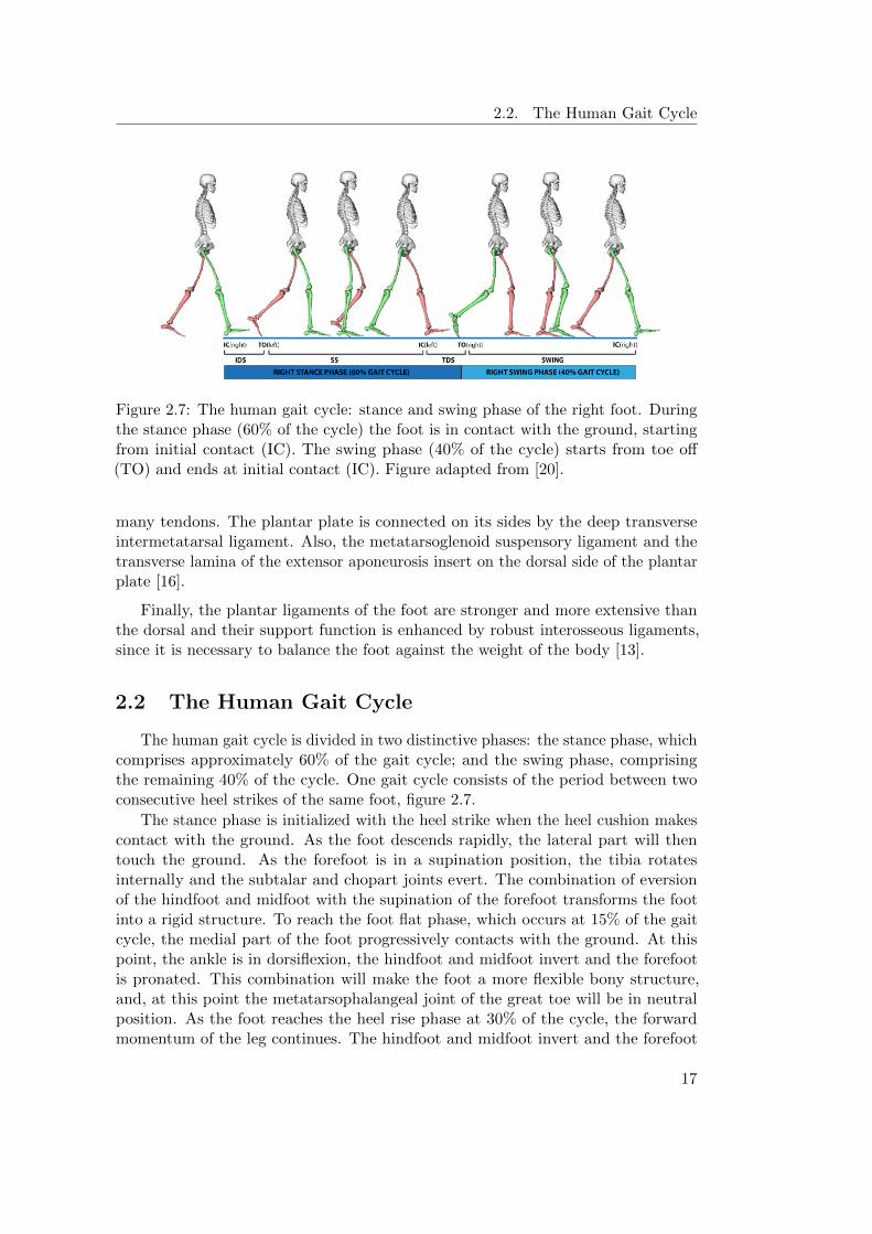
Figure 2.7: The human gait cycle: stance and swing phase of the right foot. Duringthe stance phase (60% of the cycle) the foot is in contact with the ground, startingfrom initial contact (IC). The swing phase (40% of the cycle) starts from toe o↵(TO) and ends at initial contact (IC). Figure adapted from [20].

many tendons. The plantar plate is connected on its sides by the deep transverseintermetatarsal ligament. Also, the metatarsoglenoid suspensory ligament and thetransverse lamina of the extensor aponeurosis insert on the dorsal side of the plantarplate [16].

Finally, the plantar ligaments of the foot are stronger and more extensive thanthe dorsal and their support function is enhanced by robust interosseous ligaments,since it is necessary to balance the foot against the weight of the body [13].

2.2 The Human Gait Cycle

The human gait cycle is divided in two distinctive phases: the stance phase, whichcomprises approximately 60% of the gait cycle; and the swing phase, comprisingthe remaining 40% of the cycle. One gait cycle consists of the period between twoconsecutive heel strikes of the same foot, figure 2.7.

The stance phase is initialized with the heel strike when the heel cushion makescontact with the ground. As the foot descends rapidly, the lateral part will thentouch the ground. As the forefoot is in a supination position, the tibia rotatesinternally and the subtalar and chopart joints evert. The combination of eversionof the hindfoot and midfoot with the supination of the forefoot transforms the footinto a rigid structure. To reach the foot flat phase, which occurs at 15% of the gaitcycle, the medial part of the foot progressively contacts with the ground. At thispoint, the ankle is in dorsiflexion, the hindfoot and midfoot invert and the forefootis pronated. This combination will make the foot a more flexible bony structure,and, at this point the metatarsophalangeal joint of the great toe will be in neutralposition. As the foot reaches the heel rise phase at 30% of the cycle, the forwardmomentum of the leg continues. The hindfoot and midfoot invert and the forefoot

17

2. Literature Study

Figure 2.8: Detail of the stance and swing phase of the gait cycle. Figure adaptedfrom [16]

increases the pronation position and the foot will acquire a loose status. However, asthe foot progresses to the push o↵ phase, it acts as a lever arm and maintains itsrigidity. The plantarflexion continues at the ankle and the metatarsophalangeal jointof the great toe will reach its maximum of dorsiflexion around 45%-50% of the cycle,after which it will decrease until reaching again the neutral position. Finally, the toeo↵ phase occurs at 60% of the gait cycle when the great toe breaks contact with theground, starting the swing phase [16].

The swing phase corresponds to the period in which the foot is o↵ the ground.At the beginning of this phase, the foot is accelerated and plantarflexed, then itgradually moves to dorsiflexion and eversion. In the last part of this phase, the footis decelerated, the leg rotates internally and the heel inverts. To complete the cycle,the foot progressively descends to reach the ground and when it does, the ankle is ina 90 degrees position and the heel is minimally inverted [16].

2.3 State of the Art: Existing Foot-ankle models

Throughout the years, many foot models have been developed, di↵ering in the numberand the definition of its segments. The foot models serve distinctive purposes, thus,depending on its intent, the models can be used to perform di↵erent types of analysis,such as kinematic, kinetic, forward simulation, etc. Hence, depending on the purpose,kinematic, kinetic or musculoskeletal models can be developed. This section provides

18

2.3. State of the Art: Existing Foot-ankle models

an overview of the state of the art regarding some of the di↵erent types of footmodels.

2.3.1 Kinematic and Kinetic Foot Models

Kinematics is defined to be the study of motion without considering the forcesand moments that produce that motion. Kinematics, include linear and angulardisplacements, velocities and accelerations [1]. On the other hand, kinetics is definedto be the general term given to forces that cause movement. These forces can beinternal, including muscle activity, ligaments, and force caused by friction in thejoints; or external, such as the ground reaction forces and the external loads [1].Thus, kinetics provide insight of the mechanics involved and of the strategies andcompensations of the neural system. As stated by Winter [1], a large part of the futureof biomechanics lies in kinetic analyses, because the information present permits usto make very definitive assessments and interpretations. In this sense, in order todevelop kinetic (or dynamic) foot models, a set of requirements must be fulfilled:firstly, for every foot segment, the mass, centre of mass and moment of inertia needto be defined; additionally, it is necessary to know the external forces acting on eachsegment separately.

Most of the kinematic foot models described in literature divide the foot in threesegments. The Oxford Foot Model [21] is one of them, presenting a multi-segmentapproach to measure foot kinematics during gait that was tested for its repeatabilityin healthy feet. The three segments are the hindfoot (comprising the calcaneusand talus), forefoot (metatarsals) and hallux (toes), allowing six degrees of freedombetween any pair of segments. The inter-segment angular motion was examined in thethree anatomical planes and consistent patterns and ranges of motion were detected.This model was used by Stebbins [8] where it was adapted to study children’s feet.Another three segment foot model by Okita [10] divides the foot in shank (tibia andfibula), hindfoot (calcaneus and talus) and forefoot (tarsal bones, metatarsals andtoes). In this publication the authors investigate the rigid body assumption andwhether there are di↵erences in the kinematics data from skin mounted markers andbone mounted markers. It was concluded that the shank and hindfoot behaved asrigid bodies while the forefoot violated the rigid body assumption since there wasevidence of significant di↵erences between motions of the first metatarsal and theforefoot as well as relative motion between the first and fifth metatarsals. In 1998,Rattanaprasert [22] also presented a three foot segment with a hindfoot, forefoot andhallux (in addition to a rigid leg segment) to study the e↵ects of reduced functionalactivity of the tibialis posterior muscle on the motion of the foot. The motiondi↵erences observed in the study were consistent with the expected mechanicalconsequences.

Even though the previous models satisfied the goals they were meant for, ithas been reported by Cobb [23] that significant movement occurs between thenavicular and the first ray and that the medial and lateral forefoot function somewhatindependently. The latter study investigated the e↵ect of foot posture on gaitkinematics using a four-segment foot model presenting four functional articulations:

19

2. Literature Study

hindfoot, calcaneonavicular complex, medial forefoot and first metatarsophalangealcomplex. Sawacha [24] also developed a multi-segment foot model including themidfoot, since it was considered a limitation of literature not to evaluate the midfootmotion when characterizing the foot kinematics of diabetic patients. A five-segmentfoot model was established by Tome [25], consisting of tibia, hindfoot, medial forefoot,lateral forefoot and hallux segments. The medial forefoot was defined by the firstmetatarsal and the lateral forefoot including the second through fourth metatarsals.The goal of the model was to compare the stance kinematics of patients su↵eringfrom posterior tibialis tendon dysfunction to healthy subjects. Another five-segmentfoot model is presented by Leardini [26], including the shank, calcaneus, midfoot,metatarsals and hallux to study the motion during the stance phase of gait. Caravaggi[27] used this model to investigate the relationship between foot joints mobility andplantar pressure. The study states that pressure distribution can be seen as thee↵ectiveness of the musculoskeletal system in absorbing the ground reaction forcesvia the foot and its joints. From the study it was noticed that the mean and peakpressure at the hindfoot and forefoot were negatively correlated with the amount ofmotion at the ankle and tarso-metatarsal joints. On the other hand, the pressure atthe hallux and midfoot were positively correlated with the range of motion of thejoints across the midfoot.

In 2002, MacWilliams [7] presented a model with a higher level of detail, incorpo-rating nine segments to study the kinematics and kinetics during adolescent gait. Asthis model allows to study foot kinetics, it falls into both the categories of kinematicand kinetic models. The included segments are the hallux, medial toes, lateral toes,medial forefoot, lateral forefoot, calcaneus, cuboid, talus/navicular/cuneiform andtibia/fibula. Joint angles, moments and powers were calculated for eight articulationsof the nine segments. The results indicated the complexity of gait, with specific footjoints generating power and others absorbing it. For instance, the results showed thatwhile the tarsometatarsal joint generates power, the metatarsophalangeal absorbs asimilar amount of power, therefore balancing the forefoot. Furthermore, the medialrays were found to carry higher loads, flex more and generate more power than thelateral rays, which is consistent with the fact of the first ray being structurally thelargest. Using these more detailed foot models, it was possible to have a betterunderstanding of ankle-foot kinematics and kinetics during gait. Maha↵ey [28],evaluated three di↵erent foot models in terms of their repeatability in paediatric footmotion during gait: the Oxford foot model (by Carson [21]), the 3DFoot model (byLeardini [26]) and the Kinfoot model (by MacWilliams [7]). They concluded that theOxford Foot Model showed moderate repeatability and reasonable errors except forthe hindfoot; the Kinfoot provided abundant information on the foot kinematics butthe errors were considered unacceptable; the 3DFoot model was found to o↵er anacceptable balance between repeatability and the kinematic information provided.

In 1993, Scott and Winter [29] proposed an eight-segment foot model intercon-nected by hinge joints to estimate joint kinematics and kinetics during the stancephase of the gait cycle. The plantar soft tissue of the foot was modelled as a setof springs and dampers in parallel. The structure of the model was based on theanatomy of the foot, figure 2.9. The results obtained from the kinematic and kinetic

20

2.3. State of the Art: Existing Foot-ankle models

Figure 2.9: Eight segments of the human foot model proposed by Scott and Winter,1993. Figure adapted from [29]

.

analysis allowed to classify the model as an objective tool able to quantify the motionand loading during the stance phase of walking, even though it was ascertained thatthe model is too complex for most questions regarding foot function. It was alsopointed out that the method to estimate the load at di↵erent sites of the plantarpart of the foot had many drawbacks and associated errors, since it consisted ofdecomposing the estimates of loads from walking trials where only a certain part ofthe foot landed on a force platform [29].

Abuzzahab [30] presented a three-segment kinetic model of the foot and ankleconsisting of the tibia, hindfoot, midfoot and hallux and the validation of the modelrequired kinematic, plantar pressure and ground reaction force data. The model wasonly validated for the sagittal plane.

Another kinetic foot model is presented by Bruening [31]. This model was createdsince the already existing kinetic foot models were considered too complex for clinicaluse. The model includes a shank (tibia and fibula) and three foot segments: hindfoot(calcaneus and talus), forefoot (navicular, cuboid, cuneiforms and metatarsals) andhallux (proximal and distal phalanges). Kinetic parameters were incorporated inthe model (by applying ground reaction forces to separate segments, defining theinertial properties and rigidity of the segment), and the joint moments and powerswere calculated. The results showed that the model may be used to understand andmonitor certain pathologies with only minimal impairments.

2.3.2 Musculoskeletal Foot Models

Musculoskeletal foot models include muscles and/or ligaments, being one of theirmain purposes to calculate muscle forces in combination with dynamic simulationsof motion. As such, musculoskeletal models are used to make predictive simulationsby estimating variables that cannot be directly observed and derived.

21

2. Literature Study

Figure 2.10: Musculotendon actuator model used in the work of Delp [32]. Theforces in muscles FM , and in the tendon F

T , are normalised to peak isometric muscleforce F

M

0 ; while the tendon length l

T and muscle-fiber length l

M are normalised tooptimal muscle-fiber length l

M

0 . lMT is the musculotendon length, ↵ is the pennationangle and L

T

s

is the tendon slack length. Figure adapted from [32].

One of the most notable works of the field is that of Delp [32], in which the firstmusculoskeletal model of the human lower extremity is created to study how themuscle force and moment is a↵ected by surgical interventions. With respect to thefoot, an ankle, subtalar and metatarsophalangeal joints were defined. Therefore,the foot model consisted of three rigid segments: the talus, the foot (includingthe calcaneus, navicular, cuneiforms, cuboid and metatarsals) and the toes (thephalanges). A total of forty-three musculotendon actuators were modelled in thewhole body and were represented as line segments with origin, insertion and optionalvia-points. The muscles were modelled using a three-element Hill model, with acontractile element in parallel with a passive elastic element, both in series withan elastic element. The contractile element modelled the muscle force based ona force-length and force-velocity relation. The parallel element models the elasticbehaviour of the muscle, while the series elastic element represents the non-lineartendon behaviour, figure 2.10. Thus, it was possible to compute the force and jointmoment that each muscle can develop for the di↵erent body positions by combiningthe musculoskeletal geometric data, the joint models and the musculotendon models[32].

Netptune [33], stresses the importance of examining joint loading during thenon-sagittal plane movements and also the individual muscle forces and the groundcontact force. In order to do that, the 3D musculoskeletal model of the lowerextremity with individual muscle actuators developed by Delp [32] was used and

22

2.4. Conclusion

slightly modified, with the addition of contact elements, in order to split the groundforces per segment. Moreover, the number of muscles included is lower than in theoriginal model of Delp [32], since the muscles were grouped and modelled as fourteenindependent muscle groups. Each of them with an origin and insertion point andsome of them with additional via points to represent the muscle path more accurately.The force production in muscles was also represented using Hill models. The modelwas used to analyse ankle sprain injuries.

Anderson and Pandy [34] presented a three dimensional musculoskeletal model ofthe human body to simulate normal walking. The model was actuated by fifty-fourmuscles and incorporated twenty-three DOF. Regarding the foot, it was modelledin two segments: hindfoot and toes. The path of the musculotendon actuators isbased on the work of Delp [32], and they are also modelled as a 3-element Hill-typemuscle in series with a tendon. The results of the model simulation of body segmentsdisplacement, ground reaction forces and muscles activations obtained proved to beconsistent with literature.

Finally, the most complete and detailed kinematic/kinetic model to date is theGlasgow-Maastricht foot model developed using the Anybody Modelling System[6]. The model has twenty-six segments as it considers each bone a rigid segment,twenty-six joints leading to a forty-six degrees of freedom (DOF) complex. In thisstudy [6], it was possible to recreate the foot motion during the stance phase of asubject. However, specific information on the range of motion of the bony segmentsis not presented. In the Anybody Wiki page [35], detailed information on the modelcomponents is provided, namely the list of ligaments and muscles included in themodel. It contains all the major ligament structures and muscles of foot, bothintrinsic and extrinsic. Nevertheless, information on the dynamics of the model (jointmoments and powers) and muscle forces is not freely available.

2.4 Conclusion

The human foot anatomy is presented, focusing on the foot bones, joints, intrinsicmuscles and ligaments, since understanding their anatomy is the first step towardsthe construction of a musculoskeletal foot model.

An overview of the already existing kinematic, kinetic and musculoskeletal modelsis provided. The type of foot model developed is fully dependent on its intended use.Kinematic models divide the foot into segments by grouping neighbouring bonestogether, being their main purpose the study of inter-segment movement throughcalculation of joint angles. Kinetic models, also known as dynamic models, study thekinetics involved in the generation of movement by calculating, for instance, jointmoments and powers. Musculoskeletal models are an extension of dynamic models,as muscles and/or ligaments are incorporated in order to study muscle force andmake predictive simulations.

A variety of kinematic and kinetic models, di↵ering on the number of segmentsis presented. It is observed that most models are divided into segments according tothe principal joints of the foot. However, the importance of incorporating a midfoot

23

2. Literature Study

segment is broadly conveyed. Regarding musculoskeletal models, the anatomical footstructures included and its level of detail is limited.

It is possible to conclude that biomechanical foot models have been progressivelyappearing due to the need to better understand the kinematics and forces thatcause movement. However, reproducing the real complexity of the foot into a footmodel has not been possible yet. Therefore, the development of a more detailedrepresentation contributes to this purpose.

24

Chapter 3

Methods

Chapter 3 focusses on the methods used to extend and validate the musculoskeletalfoot model. After presenting the general work-flow, the di↵erent steps of the modelconstruction are explained in detail. Next, the experimental data used for validationand the scaling of the model are explained. Finally, the methods used to validatethe model are presented and a brief conclusion is formulated.

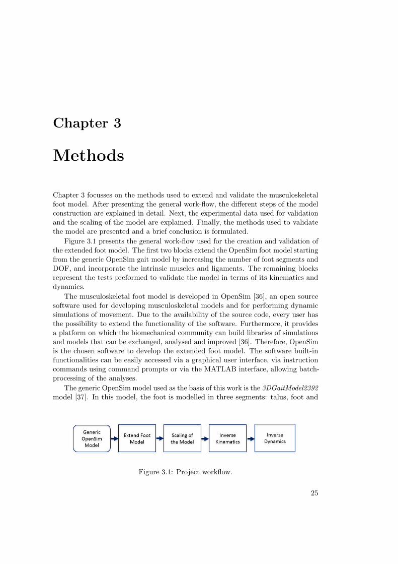
Figure 3.1 presents the general work-flow used for the creation and validation ofthe extended foot model. The first two blocks extend the OpenSim foot model startingfrom the generic OpenSim gait model by increasing the number of foot segments andDOF, and incorporate the intrinsic muscles and ligaments. The remaining blocksrepresent the tests preformed to validate the model in terms of its kinematics anddynamics.

The musculoskeletal foot model is developed in OpenSim [36], an open sourcesoftware used for developing musculoskeletal models and for performing dynamicsimulations of movement. Due to the availability of the source code, every user hasthe possibility to extend the functionality of the software. Furthermore, it providesa platform on which the biomechanical community can build libraries of simulationsand models that can be exchanged, analysed and improved [36]. Therefore, OpenSimis the chosen software to develop the extended foot model. The software built-infunctionalities can be easily accessed via a graphical user interface, via instructioncommands using command prompts or via the MATLAB interface, allowing batch-processing of the analyses.

The generic OpenSim model used as the basis of this work is the 3DGaitModel2392model [37]. In this model, the foot is modelled in three segments: talus, foot and

Figure 3.1: Project workflow.

25

3. Methods

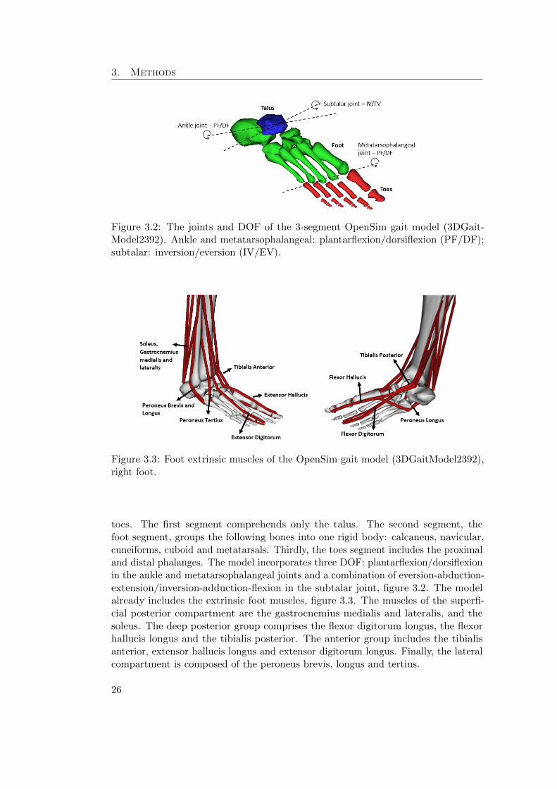
Figure 3.2: The joints and DOF of the 3-segment OpenSim gait model (3DGait-Model2392). Ankle and metatarsophalangeal: plantarflexion/dorsiflexion (PF/DF);subtalar: inversion/eversion (IV/EV).

Figure 3.3: Foot extrinsic muscles of the OpenSim gait model (3DGaitModel2392),right foot.

toes. The first segment comprehends only the talus. The second segment, thefoot segment, groups the following bones into one rigid body: calcaneus, navicular,cuneiforms, cuboid and metatarsals. Thirdly, the toes segment includes the proximaland distal phalanges. The model incorporates three DOF: plantarflexion/dorsiflexionin the ankle and metatarsophalangeal joints and a combination of eversion-abduction-extension/inversion-adduction-flexion in the subtalar joint, figure 3.2. The modelalready includes the extrinsic foot muscles, figure 3.3. The muscles of the superfi-cial posterior compartment are the gastrocnemius medialis and lateralis, and thesoleus. The deep posterior group comprises the flexor digitorum longus, the flexorhallucis longus and the tibialis posterior. The anterior group includes the tibialisanterior, extensor hallucis longus and extensor digitorum longus. Finally, the lateralcompartment is composed of the peroneus brevis, longus and tertius.

26

3.1. Model Construction

Figure 3.4: The five segments of the extended foot model: calcaneus (purple), talus(blue), midfoot (green), forefoot (yellow) and hallux (orange).

3.1 Model Construction

In order to increase the level of detail of the foot model, the first step comprehendsthe segments’ anatomical division. In parallel, it is necessary to incorporate thearchitecture of the anatomical structures that span the selected segments: the footintrinsic muscles and ligaments. Furthermore, it is necessary to acquire the muscles’and ligaments’ intrinsic properties.

3.1.1 Number of segments

In the context of the Aladyn project, the KU Leuven Foot and Ankle group (Me-chanical Engineering Department, Biomechanics Section) developed a five-segmentOpenSim foot model with five joints interconnecting the segments. The definition ofthese five segments is primarily supported by the location of the principal joints ofthe foot. Furthermore, it is consistent with the literature’s reported need to include amidfoot segment definition [10], [24], [7], [20], to represent the significant movementoccurring between the first metatarsal and the navicular [23].

The workflow to create the model comprises the following steps: (1) segmentationof CT scans, using Matlab

r software (Materialise NV, Belgium); (2) creation ofa volume mesh and (3) selection of foot landmarks in Matlab

r (Materialise NV,Belgium), followed by (4) the attribution of material properties, such as the boneand soft tissue density, in Matlab

r; thereafter, (5) the anthropometric structure iscreated in Matlab

r by computing the total mass, total volume, inertia tensor andcentre of mass of each segment; and finally (6) the model is integrated in OpenSim.

Figure 3.4 presents the five segments of the extended foot model: calcaneus, talus,midfoot, forefoot and toes. The midfoot segment includes the cuboid, navicular, andthe three cuneiforms (medial, intermedium and lateral). The forefoot segment com-prises the five metatarsal bones. Finally, the toes segment consists of all the proximaland distal phalanges. Hence, the five joints interconnecting the segments are the

27

3. Methods

Figure 3.5: The 15 degrees-of-freedom of the 5-segment model. The three rotationalmovements are incorporated at each joint: plantarflexion/dorsiflexion (PF/DF),inversion/eversion (IV/EV) and abduction/adduction (AB/AD).

ankle (interconnecting the tibia-talus segment), subtalar (talus-calcaneus), chopart(calcaneus-midfoot), tarsometatarsal (midfoot-forefoot) and metatarsophalangealjoint (forefoot-toes).

3.1.2 Number of DOF

The number of degrees-of-freedom that are incorporated in the models depend onthe purpose the models are meant to serve. In this particular case, the goal is toprovide more insight both in the design of customized insoles and in gait analysissimulations. Therefore, two models were developed based on the five segment model,each consisting of a di↵erent number of DOF interconnecting these segments: onemodel with 15 DOF and another one with 8 DOF was defined.

15 DOF Foot Model

A fifteen DOF model was created with three DOF at each of the five joints, thereforeallowing inversion/eversion, plantarflexion/dorsiflexion and abduction/adductionbetween both the parent (proximal) and child (distal) segment of the joint, figure 3.5.Even though not all these DOF are present in the foot, it was chosen to incorporatea higher level of detail into the model, to evaluate the movements that really occurin the di↵erent joints. This way, when performing simulations of movement thebehaviour of the foot could give more insight in the joint movement since therotational movement is not constrained. None of the three translational DOF wereincorporated at the joints level.

28


8 DOF Foot Model

For the 8 DOF model, the attribution of the DOF is based on the anatomical functionof the ankle-foot complex, as documented in the work of Hicks [11], figure 2.3. Inthis sense, the DOF incorporated at the joints are the following:

• Ankle joint: tibia-talus (1 DOF) - plantarflexion/dorsiflexion;

• Subtalar joint: talus-calcaneus (1 DOF) - is defined as an oblique axis, thereforecombining eversion-abduction-extension/inversion-adduction-flexion;

• Chopart joint: calcaneus-midfoot (2 DOF) - is defined by two axis, an obliqueand an anterior-posterior axis. The first axis, allows a combination of move-ments between three di↵erent planes: eversion-abduction-extension/inversion-adduction-flexion. About the anterior-posterior axis there is eversion withcoupled abduction-extension or inversion with coupled adduction-flexion;

• Tarsometatarsal joint: midfoot-forefoot (2 DOF) - is defined by two axis, the 1stray axis and the 5th ray axis, both allowing flexion-eversion/extension-eversion;

• Metatarsophalangeal joint: forefoot-toes (2 DOF) - plantarflexion/dorsiflexionand abduction/adduction.

3.1.3 Incorporation of Intrinsic Muscles

Understanding and determining the contribution of muscles to the observed motionsis an arduous task since muscles can accelerate body segments which they do notspan. Therefore, at the foot level, it is important to also include the intrinsic musclesthat span the intra-foot joints and that also have an e↵ect on the ankle control.

The incorporation of intrinsic muscles in the OpenSim model started by seekinga more insightful understanding of muscle architecture. It is defined by Kura [18]as the arrangement of muscle fibers relative to the axis of force generation andits understanding has significance for, among others, biomechanical modelling andanalysis of normal foot function. The physiologic cross-sectional area (PCSA) of themuscle, which measures the number of sarcomeres in parallel with the pull angle ofthe muscle [1], is considered to be one of the most important parameters since it isbelieved to be directly related to isometric muscle force [38], [18], which is the forcegenerated by the muscle in a static position without changing its length [39].

The choice of the muscles included in the model was primarily based on thenumber of segments the muscles span. Hence, only the intrinsic muscles that havetheir origin, insertion and via points in two or more of the five segments defined in themodel were included. Intrinsic muscles within a rigid segment would have no addedvalue, since there is no relative movement and thus no moment generating capacityof the muscle. The geometry and placement of the muscles in the model is based onscientific literature [18], [16], [13]. Figure 3.6 shows the OpenSim extended modelwith the intrinsic muscles that are included. On the left side, the intrinsic muscles ofthe dorsal part of the foot as well as the first layer of the plantar intrinsic muscles are

29

3. Methods

Figure 3.6: Foot intrinsic muscles incorporated in the extended OpenSim model.

presented. The right side shows the second and third layer of the plantar intrinsicmuscles. Tables A.2, A.3 and A.4, in Appendix A, list more detailed informationon the respective segment where the origin, via and insertion points of the intrinsicmuscles are located.

OpenSim provides di↵erent classes of muscles, and with each class a di↵erentmathematical approach for modelling the muscle functionality. These classes canbe very complete, with modelling the force-length and force-velocity behaviour ofthe muscle structure. However, this requires that specific parameters to describemuscle function, such as the maximum isometric force, the optimal fiber length orthe maximum contraction velocity need to be known. However, this informationis not freely available in literature. Therefore, it is chosen to model the intrinsicmuscles as a simple ”Path Actuator”. This muscle model describes the muscle forceas a ratio of an optimal force transferred to the interconnected bodies via a geometrypath. Therefore, this class requires as input the optimal force of the actuator andthe geometry path, represented by a set of points (origin, insertion and optional viapoints). The main reason for using this class is the fact that it allows the creation

30


of as many path points as needed to define the muscle path, and because it is onlyrequired to provide the optimal force of the muscle. These geometrical and muscleforce information can be retrieved from literature. It would not be possible to usea di↵erent modelling class due to the limited available information on the intrinsicproperties of the foot intrinsic muscles, however, for the purposes the extended modelis being developed, the path actuator is a fair representation of the intrinsic muscles.In this sense, the parameters used for modelling the path actuators are collectedfrom the work of Kura et al., 1997 since it is one of the very few in depth studies ofthe intrinsic muscles of the foot. A table with the referred parameters can be foundin Appendix A. The integration of all the intrinsic muscles is done in an automatedway using Matlab

r.

3.1.4 Incorporation of Ligaments

Incorporating ligamentous structures in a kinetic foot model significantly increasesthe level of joint stabilization. Commonly, ligaments are not included in multi-segment foot models, since most models’ purpose is to explain muscle function andfor that reason ligaments are not included. Nevertheless, ligaments are responsiblefor stabilizing the foot joints by connecting neighbouring bones together, and willtherefore a↵ect the muscle balance.

Ligaments are considered to be viscoelastic structures, meaning that their me-chanical behaviour depends on time and on the load-history [40]. The ligaments arepassive elements whose primary purpose is to constrain motion. They are graduallystretched as displacement between their origin and insertion points occurs, and returnto their original shape when the tension is no longer applied. Ligament behaviour isnon-linear as demonstrated by the ligament force-length curves documented whenapplying constant strain rates [40]. This happens because the collagen fibers thatcompose the ligaments are recruited gradually as load increases [41]. Figure 3.7presents the characteristic force-displacement curve of ligaments (also referred to asforce-length curve). The force length curve can be subdivided in three regions: thetoe region, which is non-linear and occurs for low strain values, the elastic region,which displays a linear behaviour and the plateau region, that leads to failure of theligament tissue.

The process of incorporating ligaments follows the same work-flow as the in-corporation of the intrinsic muscles. The first step consisted of understanding thearchitecture of the ligaments and their location in the foot. Based on this informa-tion, it was possible to decide which ligaments are appropriate to include in thefive-segment foot model, since, analogously to the case of the intrinsic muscles, it isonly advantageous to include ligaments that span joints that are modelled in theextended OpenSim foot model. The ligament geometry path is described by a pointset (origin, insertion and optional via points), in the same way as for the intrinsicmuscles.

Figures 3.8 and 3.9 present the ligaments incorporated in the OpenSim footmodel. The first figure shows the medial and laterial view of the foot with therespective ligaments. Figure 3.9 presents the ligaments in the plantar aspect of the

31

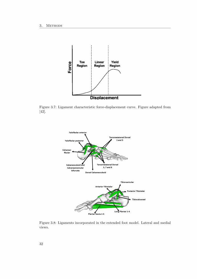
3. Methods

Figure 3.7: Ligament characteristic force-displacement curve. Figure adapted from[42].

Figure 3.8: Ligaments incorporated in the extended foot model. Lateral and medialviews.

32


Figure 3.9: Ligaments incorporated in the extended foot model. Plantar and dorsalviews.

foot except for the upper right part of the figure that shows the dorsal ligamentsthat are included in the model. Their placement in the model is according to whatis reported in literature [19] [16] [13]. Tables B.2, B.3, B.4 and B.5, in AppendixB, list the ligaments incorporated in the model and the respective body segment towhich their origin, via and insertion points are attached to.

In OpenSim it is possible to model ligaments using the class Ligament. Theclass requires as input the resting length of the ligament, which is the length at zeroload (zero strain), the force length curve of the ligament and PCSA force, which isused to scale the force-length curve. This force-length curve models the non-linearbehaviour of the ligament. It relates the ligament force to the normalized length ofthe ligament:

L

norm

=L

L0(3.1)

Being L0 the resting length and L the ligament length.According to the OpenSim ligament definition, the strain can be written as:

" =L� L0

L

(3.2)

33

3. Methods

In this way, when the ligament length is shorter than the resting length no forceis generated, whereas when the ligament is stretched beyond the resting length, thereis force generation.

As mentioned above, the ligament elasticity is generally non-linear. Therefore, itis necessary to construct the ligament force-length curve including the non-linearbehaviour. Hence, based on [43], a fourth order polynomial form equation is used toconstruct the force-length curve:

F = A+B"+ C"

2 +D"

4 (3.3)

Being A = 0 and B = k

init

, which is the initial sti↵ness and the sti↵ness is defined

as: k =F1

" ⇤ L0. Equation 3.3 is then derived with respect to the strain, 3.4. This

way, it is possible to solve the equation for each ligament present in the model, tofind the missing variables, C and D.

dF

d"

= B + 2C"+ 4D"

3 (3.4)

"

2nom

"

4nom

2"nom

4"3nom

�⇥C

D

�=

F

nom

� k

init

⇤ "nom

k

nom

� k

init

�

The parameters that define the non-linearity of the ligament force-length curveare the relative initial sti↵ness, a0, and the relative sti↵ness at nominal strain, a1.In this sense, the initial sti↵ness, k

init

, is scaled by being multiplied by the relativeinitial sti↵ness, a0 and by the respective resting length, L0. Similarly, the nominalsti↵ness, k

nom

, is multiplied by the relative sti↵ness at nominal strain, a1 and by theligament resting length, L0. Therefore, a0, defines the slope of the force-length curveat resting length (at the beginning of the curve) interpolating the curve betweenzero and the linear part of the force length curve, while a1 interpolates the curve inthe yield region [43]. It is then possible to compute the force-length curve of eachligament by interpolating the force values. The force-length curve is normalised bydividing every force value by the PCSA force. It is also important to mention thatthe yield region of the characteristic ligament force-length curve was modelled to beconstant. Table B.1 in Appendix B lists all the values, retrieved from literature [44],[45], [46], [47], [48], [49], [19], that were used as input to the variables mentionedabove. The time and load history properties of the ligaments are not taken intoaccount in this approach.

3.2 Experimental Data Collection

Experimental data, collected during the work of Burg [20], was used in order to scaleand validate the foot model. The data comprised motion capture data (200 Hz) fromfive healthy subjects walking barefoot, using ten infra-red Vicon cameras (Vicon r,Oxford Metrics, UK) to track the motion of a sixty-five skin-mounted marker set.From the sixty-five markers, eighteen are positioned on each foot, figure 3.10, making

34

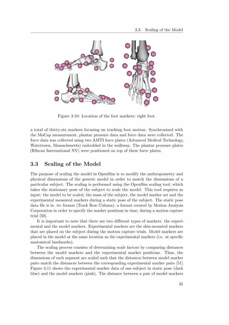
3.3. Scaling of the Model

Figure 3.10: Location of the foot markers: right foot.

a total of thirty-six markers focusing on tracking foot motion. Synchronised withthe MoCap measurement, plantar pressure data and force data were collected. Theforce data was collected using two AMTI force plates (Advanced Medical Technology,Watertown, Massachusetts) embedded in the walkway. The plantar pressure plates(RSscan International NV) were positioned on top of these force plates.

3.3 Scaling of the Model

The purpose of scaling the model in OpenSim is to modify the anthropometry andphysical dimensions of the generic model in order to match the dimensions of aparticular subject. The scaling is performed using the OpenSim scaling tool, whichtakes the stationary pose of the subject to scale the model. This tool requires asinput: the model to be scaled, the mass of the subject, the model marker set and theexperimental measured markers during a static pose of the subject. The static posedata file is in .trc format (Track Row Column), a format created by Motion AnalysisCorporation in order to specify the marker positions in time, during a motion capturetrial [50].

It is important to note that there are two di↵erent types of markers: the experi-mental and the model markers. Experimental markers are the skin-mounted markersthat are placed on the subject during the motion capture trials. Model markers areplaced in the model at the same location as the experimental markers (i.e. at specificanatomical landmarks).

The scaling process consists of determining scale factors by comparing distancesbetween the model markers and the experimental marker positions. Thus, thedimensions of each segment are scaled such that the distances between model markerpairs match the distances between the corresponding experimental marker pairs [51].Figure 3.11 shows the experimental marker data of one subject in static pose (darkblue) and the model markers (pink). The distance between a pair of model markers

35

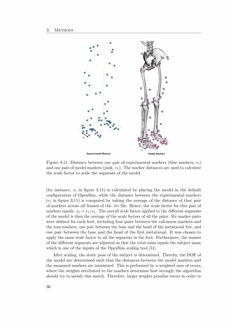
3. Methods

Figure 3.11: Distance between one pair of experimental markers (blue markers, e1)and one pair of model markers (pink, v1). The marker distances are used to calculatethe scale factor to scale the segments of the model.

(for instance, v1 in figure 3.11) is calculated by placing the model in the defaultconfiguration of OpenSim, while the distance between the experimental markers(e1 in figure 3.11) is computed by taking the average of the distance of that pairof markers across all frames of the .trc file. Hence, the scale factor for this pair ofmarkers equals: s1 = e1/v1. The overall scale factor applied to the di↵erent segmentsof the model is then the average of the scale factors of all the pairs. Six marker pairswere defined for each foot, including four pairs between the calcaneus markers andthe toes markers, one pair between the base and the head of the metatarsal five, andone pair between the base and the head of the first metatarsal. It was chosen toapply the same scale factor to all the segments in the foot. Furthermore, the massesof the di↵erent segments are adjusted so that the total mass equals the subject mass,which is one of the inputs of the OpenSim scaling tool [51].

After scaling, the static pose of the subject is determined. Thereby, the DOF ofthe model are determined such that the distances between the model markers andthe measured markers are minimized. This is performed by a weighted sum of errors,where the weights attributed to the markers determine how strongly the algorithmshould try to satisfy this match. Therefore, larger weights penalize errors in order to

36

3.4. Model Validation

match the model markers with the experimental markers more closely [51]. In thissense, larger weights were attributed to the markers located on the shoulders of thesubject and on the calcaneus marker cluster.

The path actuators and intrinsic muscles of the model also need to be scaledsince these structures depended on the length of the segments. The scaling tool ofversion 3.2 of OpenSim scales the geometry of these structures, however, it does notscale the length-dependent properties of the ligaments. In a post-processing step,the resting length of the ligaments are scaled in Matlabr. Knowing the geometryof the scaled model, the ligament length L

ligGeneric

and resting length L0Generic

ofthe generic model, it is possible to compute the resting length of the scaled model,based on the length of the ligament at default position L

ligScaled

:

L0Scaled =L0Generic

L

ligGeneric

⇥ L

ligScaled

(3.5)

In the OpenSim scaling tool it is possible to specify if the model markers shouldbe adjusted to match the experimental markers’ locations. This is done by loadingthe same .trc file containing the experimental marker locations in order to find theproper set of joint angles to match the subject’s pose. It is done by averaging allthe experimental markers over the specified time interval and an inverse kinematicsproblem is solved [52]. Both the 15 DOF and the 8 DOF models were scaled using thesame marker set. For the 8 DOF model, the option of adjusting the model markersto the experimental marker location was chosen, while for the 15 DOF model it wasnot. For the 15 DOF model, the adjusted marker set obtained for the 8 DOF modelwas used. As a result, the di↵erences observed during inverse kinematics analysiswould not be due to di↵erences in scaling. In this way, both models were identicallyscaled.

3.4 Model Validation

The constructed and scaled model was validated by performing inverse kinematicsand inverse dynamics analysis to compare the results with literature. In this sense,the following subsections present the methodologies used to perform the kinematicsand dynamics analysis.

3.4.1 Inverse Kinematics

Inverse kinematics analysis estimates joint angles based on measured trajectories ofskin-mounted markers. The Kalman Smoother algorithm, by De Groote [53], wasthe tool used to perform inverse kinematics analysis. Compared to other techniquesthat estimate joint kinematics, the Kalman Smoother algorithm uses completemarker trajectories to make the estimations instead of basing only on partial markertrajectory information [53]. It computes the joint angles by stepping through eachtime frame and positioning the model in a pose that best matches the experimentalmarker and coordinate errors information. It solves a weighted least squares problemand its solution aims at minimizing the marker errors [54].

37

3. Methods

The Kalman Smoother algorithm consists of two consecutive steps: a Kalmanfilter to estimate the joint kinematics at a given time instant, t

i

, using markertrajectory information only until t

i

; and a backward recursion going from the lastinstant of measured marker trajectory until t

i

. Hence, the resulting estimates ofthe Kalman Smoother are computed based on all the available information. Thisinformation includes all the complete marker trajectory, the process model, whichdescribes the expected time evolution of the joint kinematics for each DOF, andthe measurement model, which relates the joint kinematics to the measured markerpositions [53].

The input needed to run the Kalman Smoother is the experimental marker datacollected during the motion capture trials. It is also necessary to provide a scaledmusculoskeletal model containing the definition of the marker set used, as well asthe weights associated with each marker. The higher the weight of the marker, themore the marker error is minimized. The marker weight attribution is, therefore,a crucial step of the inverse kinematics analysis. It is necessary to assign the footmarker weight di↵erently for each trial, since the reliability of the markers variesfrom trial to trial, as skin motion artefacts may arise. During the experimental trialthere is relative movement of the markers within the segment due to skin motion,thus, the markers that present less displacement throughout the trial are consideredmore accurate.

The foot marker weights are assigned as follows: for each time step and for eachsegment, the relative distances between each marker of the segment is calculated.Subsequently, it is possible to calculate the inter-marker distance (IMD) of each pairof markers in one segment by subtracting the minimum distance from the maximumdistance observed between those markers. Then, the average IMD for each markercan be calculated. Therefore, for every segment, the average and the maximumvalues of the IMD were determined. Due to the high number of markers placedon the foot and the consequent di�culties in tracking each marker correctly, theweight range assigned to these markers is limited between 0.25 and 2. The weightsare assigned linearly, figure 3.12, being the markers that present the least relativedisplacement assigned with an higher weight value and the markers presenting moremotion with a lower weight. Figure 3.12, is a graphical representation of the weightattribution algorithm. If the maximum IMD of the segment is larger than the upperlimit (2 cm) there are two cases: the IMD of the marker is equal or larger than theaverage IMD, red line, or the IMD of the marker is smaller than the average IMD ofthe segment, blue line. On the other hand, if the maximum IMD of the segment isequal or smaller than the upper limit there are also two possible cases: the IMD ofthe marker is equal or larger than the average IMD of the segment, green line, orthe IMD of the marker is smaller than the average, blue line. It is important to notethat the average IMD varies from segment to segment, therefore it does not have afixed position in the graph, and it is not necessarily smaller than the upper limit.

Figure 3.13a shows the IMD, in mm, during one trial and figure 3.13b the weightattribution according to the IMD. Regarding the markers of the upper body andleg, the same weight was attributed to all the trials and all the subjects. Thesemarkers are assigned a higher weight compared to most of the foot markers, since

38


Figure 3.12: Graphical representation of the linear marker weight attribution for thedi↵erent cases (coloured lines). If the IMD of the segment is larger than an imposedlimit (upper limit - 2cm): the blue line represents the weight assignment in case theIMD of the marker is smaller than the average IMD of the segment, and the red linein case the marker IMD is equal or larger than the average IMD of the segment. If,on the other hand, the marker IMD is equal or smaller than the upper limit: thegreen line in case the marker IMD is equal or larger than the average IMD of thesegment and the blue line in the opposite case.

these markers are easily tracked and present small relative displacement during thetrials.

Regarding the 15 DOF model, due to having all three rotational degrees-of-freedom in each joint, some of the movements allowed are not anatomically possible.Besides that, the model has more freedom to try to solve the inverse kinematics,generating results that are not, at times, realistic. One of these is the motion ofthe talus, since skin-mounted markers are not capable of tracking its movement.Therefore, three model markers were added to the model markers’ set for the 15DOF model. The markers were placed on the anterior aspect of the talus; on thelateral aspect and on top of the talus (coinciding with the ankle joint).

After having the resulting motion file obtained from the Kalman Smoother, anextra analysis, named Body Kinematics, was performed to retrieve the position andorientation of the bodies with respect to the anatomical planes. It is necessaryto perform this extra analysis as the Kalman Smoother retrieves the angles ofall the DOF, however, as the 8 and the 15 DOF models have di↵erent joint axisdefinitions, it is not possible to compare the angles. Therefore, by examining themotion relatively to the anatomical planes (sagittal plane- flexion/extension; frontal

39

3. Methods

Figure 3.13: (a) Example of the IMD for one trial and the respective marker weightattribution, (b).

plane- inversion/eversion; transverse plane- adduction/abduction), it is possible tocompare both models. Consequently, this analysis calculates the orientation andposition of the centre of mass of each body based on the gait pattern calculated viathe Kalman Smoother. In this way, by subtracting the orientation of each consecutivepair of segments, it is possible to obtain the relative movement, in degrees, betweenthe segments. This is also the approach used in literature.

The inverse kinematics analysis were performed using the experimental data offive subjects, with four trials per subject. It was done for both the 8 DOF modeland the 15 DOF model, and their results were compared. Only the stance phase isstudied as it is the most relevant for the purpose of the extended musculoskeletalmodel, especially to describe the contact of the foot with the ground. For the analysis,right and left foot kinematics were combined for each trial. Therefore, a total of40 trials is analysed per model: five subjects, four trials per subject and per foot.After observing the output of the inverse kinematics analysis, it was noticed that forsome trials the Kalman Smoother algorithm did not find an optimal solution. Thiswas observed for seven out of forty trials (7/40) performed with the 15 DOF modeland for four out of forty trials (4/40) with the 8 DOF model. Consequently, it wasdecided not to take these trials into account. The mean of the di↵erent trials persubject was calculated and, subsequently, the mean and standard deviation (SD) ofthe five subjects were determined.

40


3.4.2 Inverse dynamics

Inverse dynamics computes the net forces and torques at each joint underlying aparticular movement [55]. The inverse dynamics tool of OpenSim was used. It takesthe motion (the output of the inverse kinematics) and the external loads applied tothe model as input to determine the generalized forces.

The principle behind inverse dynamics is expressed by the classical equation ofmotion that can be written, in the inverse dynamics sense [56], as follows:

M(q)q + C(q, q) +G(q) = ⌧ (3.6)

With N the number of degrees-of-freedom, q, q, q 2 R

N represents the vectorsof generalized positions, velocities and accelerations, respectively; M(q) 2 R

N⇥N

is the system matrix; C(q, q) 2 R

N is the vector of Coriolis and centrifugal forces;G(q) 2 R

N is the vector of gravitational forces and ⌧ 2 R

N is the vector of generalizedforces that must be determined [56]. All the terms of the first part of the equationare known, since the motion of the model is completely defined by the position,orientation, velocity and acceleration of the centre of mass of the segments [56].Therefore, the inverse dynamics solves the equations of motion in order to find themissing term: the net forces and torques for each joint. In order to maximally exploitthe inverse dynamic analyses for the complex foot model, the ground reaction forcesneed to be split and applied to the respective segments, since the force is acquired asone single vector applied only in one segment.

Splitting the Ground Reaction Forces

It is, therefore, necessary to subdivide the ground reaction forces acting on the footaccording to the number of foot segments of the model. The extended foot modelconsists of five segments, but only four of them are in contact with the ground: morespecific, calcaneus, midfoot, forefoot and toes. The subdivision of the ground reactionforces was performed using an algorithm developed by the KU Leuven Foot andAnkle group (Mechanical Engineering Department, Biomechanics Section), based onthe plantar pressure data.

The simultaneously measured plantar pressure provides information on the verticalforce component and the point of application of this force component. By subdividingthe plantar pressure in four regions, figures 3.14a and 3.14b, the vertical force andthe point application are subdivided over the four segments. For the two other forcecomponents (medio-lateral and antero-posterior), it is assumed that they relate tothe measured force with the same ratio as the vertical forces. Therefore, the groundreaction forces are decomposed proportionally to the pressure registered for eachsegment. The division of the pressure information into the di↵erent segments isdone manually by selecting four points in the pressure map containing the maximalplantar pressure for all time steps. It is done in a graphical user interface (GUI) inMatlab

r by choosing four points in the following regions: calcaneus, head of the fifthmetatarsal, head of the first metatarsal and toes. Figure 3.14a shows an exampleof one trial with four chosen points and the consequent division of the segments.

41

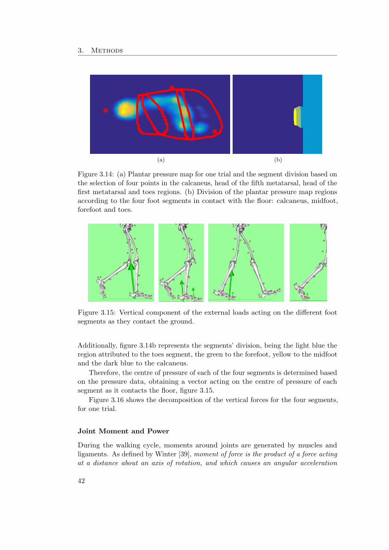
3. Methods

(a) (b)

Figure 3.14: (a) Plantar pressure map for one trial and the segment division based onthe selection of four points in the calcaneus, head of the fifth metatarsal, head of thefirst metatarsal and toes regions. (b) Division of the plantar pressure map regionsaccording to the four foot segments in contact with the floor: calcaneus, midfoot,forefoot and toes.

Figure 3.15: Vertical component of the external loads acting on the di↵erent footsegments as they contact the ground.

Additionally, figure 3.14b represents the segments’ division, being the light blue theregion attributed to the toes segment, the green to the forefoot, yellow to the midfootand the dark blue to the calcaneus.

Therefore, the centre of pressure of each of the four segments is determined basedon the pressure data, obtaining a vector acting on the centre of pressure of eachsegment as it contacts the floor, figure 3.15.

Figure 3.16 shows the decomposition of the vertical forces for the four segments,for one trial.

Joint Moment and Power

During the walking cycle, moments around joints are generated by muscles andligaments. As defined by Winter [39], moment of force is the product of a force actingat a distance about an axis of rotation, and which causes an angular acceleration

42

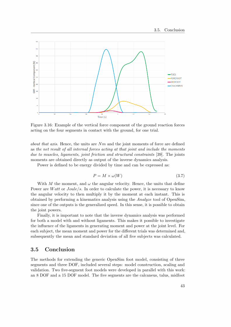
3.5. Conclusion

Figure 3.16: Example of the vertical force component of the ground reaction forcesacting on the four segments in contact with the ground, for one trial.

about that axis. Hence, the units are Nm and the joint moments of force are definedas the net result of all internal forces acting at that joint and include the momentsdue to muscles, ligaments, joint friction and structural constraints [39]. The jointsmoments are obtained directly as output of the inverse dynamics analysis.

Power is defined to be energy divided by time and can be expressed as:

P = M ⇥ !(W ) (3.7)

With M the moment, and ! the angular velocity. Hence, the units that definePower are Watt or Joule/s. In order to calculate the power, it is necessary to knowthe angular velocity to then multiply it by the moment at each instant. This isobtained by performing a kinematics analysis using the Analyze tool of OpenSim,since one of the outputs is the generalized speed. In this sense, it is possible to obtainthe joint powers.

Finally, it is important to note that the inverse dynamics analysis was performedfor both a model with and without ligaments. This makes it possible to investigatethe influence of the ligaments in generating moment and power at the joint level. Foreach subject, the mean moment and power for the di↵erent trials was determined and,subsequently the mean and standard deviation of all five subjects was calculated.

3.5 Conclusion

The methods for extending the generic OpenSim foot model, consisting of threesegments and three DOF, included several steps: model construction, scaling andvalidation. Two five-segment foot models were developed in parallel with this work:an 8 DOF and a 15 DOF model. The five segments are the calcaneus, talus, midfoot

43

3. Methods

(cuboid, navicular and cuneiformia), forefoot (metatarsals) and toes (phalanges).The foot model was further extended by the incorporation of intrinsic muscles andligaments. Their location in the foot and characteristic parameters were retrievedfrom literature and implemented in the OpenSim model in an automated way, usingMatlab

r. The ligament force-length curve was modelled based on literature, takingthe form of a fourth order polynomial equation, where the non-linear mechanicalbehaviour of the ligament was taken into account.

Experimental motion capture, force and plantar data of five healthy subjects,gathered during the work of Burg [20], was used to scale and validate the extendedmusculoskeletal foot models.

Finally, the methods utilized for the model validation were the inverse kine-matics and inverse dynamics analysis. The most optimal marker tracking weightis determined automatically. For the inverse dynamics, the ground reaction forceswere subdivided according to the foot segment in contact with the ground, basedon plantar pressure data. Given the output of the inverse kinematics (joint angles)and the output of the inverse dynamics ( joint moments), the joint powers werecalculated.

44

Chapter 4

Results

The results obtained from the inverse kinematics and inverse dynamics analysis arepresented. The first section of the chapter presents the kinematic results both forthe 15 DOF model and the 8 DOF model. The next section presents the dynamicresults, joint moments and powers, obtained for the 8 DOF model.

4.1 Kinematics

The kinematic results were compared with the results obtained in the study con-ducted by Lundgren [57]. Their results are considered a golden standard since thekinematic data was collected using in vivo bone-anchored markers. This eliminatedthe occurrence of skin movement artefacts that is seen using skin-mounted markers.Furthermore, since the marker pins are drilled individually into the foot bones, it ispossible to assess the movement between the bones, having a better understandingof the joint motion. Moreover, using this approach, it is possible to track the motionof the talus, which is inaccessible using skin-mounted markers. Nine bones werestudied: tibia, fibula, talus, calcaneus, navicular, cuboid, medial cuneiform, first andfifth metatarsal. It is the first in vivo bone-anchored marker study to investigatethe movement within the midfoot and forefoot. Nevertheless, as no bone-pins wereinserted into the phalanges, the metatarsophalangeal motion was not studied.

Figure 4.1 presents the inverse kinematics results obtained with the 8 DOF model(green), the 15 DOF model (red) and the results of Lundgren [57] (blue). On theX axis the percentage of the stance phase of the gait cycle is displayed and the Yaxis represents the angles between the two bodies, in degrees. The first column offigures shows the eversion/inversion rotation, where the positive values correspondto eversion and the negative to inversion. In the second column, the plantarflex-ion/dorsiflexion movement is shown, being plantarflexion the positive values anddorsiflexion the negative. The third column presents adduction, positive values,and abduction, negative values. The movement, represented by eversion/inversion,plantarflexion/dorsiflexion and abduction/adduction, was calculated for the follow-ing pairs of bodies: tibia-talus, talus-calcaneus, calcaneus-midfoot, talus-midfoot,midfoot-forefoot and forefoot-toes. For each subject and each foot, the mean of the

45

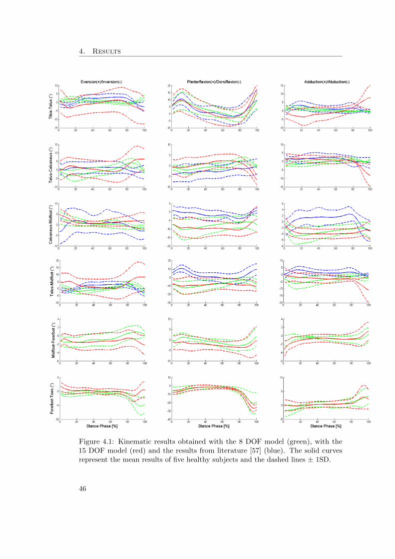
4. Results

Figure 4.1: Kinematic results obtained with the 8 DOF model (green), with the15 DOF model (red) and the results from literature [57] (blue). The solid curvesrepresent the mean results of five healthy subjects and the dashed lines ± 1SD.

46

4.2. Dynamics

four trials was calculated. Then, by taking the mean of all trials, the mean and thestandard deviation (SD) of all subjects was determined and it is presented in figure4.1.

Firstly, by inspecting figure 4.1, it is possible to observe that the 15 DOF model(red curves) presents more inter-subject variability and a larger range of motionin most of the plots than the 8 DOF model (green curves), except for the inter-segment joint angles between the forefoot-toes and calcaneus-midfoot segments.Secondly, when comparing the 8 DOF model (green curves) with literature [57] (bluecurves), the curve profiles, as well as the range of motion are very consistent. Themain di↵erences are observed in the calcaneus-midfoot and talus-midfoot segments.Regarding the calcaneus-midfoot, literature presents a larger range of motion forthe eversion/inversion movements, while for the plantarflexion/dorsiflexion andadduction/abduction the curves are somewhat shifted. The same can be found forthe talus-midfoot segments. However, it is important to note that the axis scale israther small, therefore overemphasising the di↵erences between the curves. It is alsonoteworthy that in literature the comparison is made for the calcaneus in relation tothe cuboid, while in the developed models the comparison is between the calcaneusand midfoot. The same happens for the talus and midfoot as in literature the motionis defined between the talus relative to the navicular.

Since the work of Lundgren [57] did not include bone pins in the phalanges, itwas not possible to compare the results obtained for the metatarsophalangeal joint.Furthermore, the data of the relative movement of the midfoot-forefoot was notavailable. Nonetheless, it was possible to compare the results with the work of Burg[20], being the ranges of motion and curve profiles very similar.

4.2 Dynamics

After the kinematic analysis, it was decided to proceed the dynamics analysis withonly the 8 DOF model, since this model generated kinematic results that were morecomparable to literature. As mentioned in the last chapter, the inverse dynamicsanalysis was performed for both a model with and without ligaments, allowing toinvestigate the influence of the ligaments in generating moment and power at thejoint level.

Validating the results obtained for the joint moments and powers can only bedone with confidence for the ankle joint, since, to date, there are not many otherkinetic foot models with such level of detail. Therefore, the ankle joint moment andpower were compared with the results obtained by Burg [20].

Figure 4.3 presents the moment normalised by the mass of each subject as apercentage of the gait cycle. The blue curves represent the resulting joint momentstaking the ligaments into account and the green curves without considering them.

Observing figure 4.3 and comparing it to the results obtained by Burg [20], figure4.2, it is possible to state that the profile of the ankle joint curve is in accordancewith literature. At the beginning of the stance phase the vertical component of theground reaction force is aligned with the ankle joint, therefore, a very small moment

47

4. Results

Figure 4.2: Ankle moment and power obtained by Burg [20]. Figure adapted from[20].

(positive in this case) is induced. After that, the moment increases reaching themaximum moment at push o↵. It is also possible to notice di↵erences in the momentcaused by the presence of ligaments, figure 4.3. Only for the ankle and subtalar jointthere is no apparent di↵erence.

Figure 4.4 displays the normalised joint power for each one of the eight degrees-of-freedom. Similarly to the moment, the ankle power curve profile follows the patternsfound in literature [20]. Negative values indicate power absorption and positive valuespower generation. The chopart joint, both the oblique and the anterior-posterioraxis, stands outs due to presenting an oscillating and somewhat large range ofmotion. Finally, it is also noteworthy that the axis of the graphs, in figures 4.3 and4.4, are scaled to di↵erent ranges in order to clearly observe the curves’ patterns.Nevertheless, the moments and powers are considerably larger at the ankle joint incomparison with the remaining joints.

4.3 Conclusion

Experimental data of five healthy subjects were used to perform the inverse kine-matics analysis. The results of the inverse kinematics analysis are very consistentwith literature [57] [20]. The most notable dissimilarities were verified betweenthe calcaneus-midfoot and talus-midfoot segments. Regarding the two models incomparison: the 8 DOF model revealed to be more consistent with literature andpresented less inter-subject variability.

The 8 DOF model was, therefore, the chosen to continue with the inverse dynamicsanalysis. The joint moments and powers were compared with literature [20]. Theresults were also very consistent. When comparing the dynamic results with ligamentsand without, it was noticed that for the ankle and the subtalar joint the curve profilesobtained were exactly the same. For the remaining degrees-of-freedom, di↵erentmoments and powers were verified.

48

4.3. Conclusion

Figure 4.3: Joint normalised moments (Nm/Kg) obtained for the 8 DOF model, withand without including ligaments in the inverse dynamic analysis, blue and greencurves, respectively. The solid lines represent the mean moment of the five subjectsand the dashed lines ± 1SD.

49

4. Results

Figure 4.4: Joint powers (W/Kg) obtained for the 8 DOF model, with and withoutincluding ligaments in the inverse dynamic analysis, blue and green curves, respec-tively. The solid lines represent the mean power of the five subjects and the dashedlines ± 1SD.

50

Chapter 5

Discussion

In this chapter, the results obtained are analysed and discussed. The first sectionfocus on the kinematic results and the required improvements. More specifically,the marker weight attribution and the comparison between the 8 DOF and 15 DOFmodels are addressed. The next sections discuss the dynamic results. Finally, futuredevelopments, such as the static optimization, are briefly presented.

5.1 Kinematics

In this first section, the kinematics behaviour of the extended ankle-foot model isdiscussed. This comprises first the use of the marker weight attribution for modelscaling and inverse kinematics analysis. Secondly, the di↵erences in the inversekinematics results of the 8 DOF and 15 DOF model are discussed.

Marker Weight Attribution

Experimental testing is commonly subjective to measurement errors, due to equipmentlimitations as well as human and environment induced errors. During the motioncapture data acquisition performed by Burg [20], a high number of experimentalmarkers (18) were placed on the foot in order to track the motion of its bones. Thisresults in two specific challenges: on one hand, a high number of markers needto be placed in an accurate way to track the foot motion; on the other hand, itis challenging to place such a high amount of markers close to each other. Thisproximity may cause di�culties for the cameras to distinguish the markers. Inspecific instances, some of the markers are covered either by other markers or bythe opposite foot/leg, and are, therefore, not visible to the cameras. Whereas theexperimental markers are supposed to be placed in specific anatomical locations, themarker placement is not always accurate and some landmarks are less accessiblethan others. Furthermore, skin motion artefact also contributes to measurementerrors. Ideally, the marker weighting used should accommodate for these e↵ectsand di↵erentially attribute marker weights depending on the relative stability ofthe individual markers. Therefore, an algorithm was developed for determining thetracking weight of individual markers. This was inversely related to the inter-segment

51

5. Discussion

displacement of the marker throughout the trial, as described in chapter 3. It ishowever important to recognize the high sensitivity of both models to the markerweight attribution during the inverse kinematics analysis. Changes in marker weightwere, in some cases, found to have a substantial impact in the result obtained fromthe Kalman Smoother. Therefore, the weight attribution algorithm can still beimproved. As mentioned in the last chapter, for the 15 DOF model, 7 out of 40trials had to be removed after the kinematics analysis whereas 4 out of 40 trials wereremoved for the 8 DOF model as the Kalman Smoother could not find a solutionfor the inverse kinematics. The higher level of measurement error in these trials,introducing noise to the marker data, may be a possible explanation for the failing ofthese trials. It is also noteworthy that the four trials removed for the 8 DOF modelwere from the same subject and same foot, hence the problem is more likely to lie inthe experimental data acquisition of that particular subject rather than in the model.On the other hand, the removed trials of the 15 DOF model were from di↵erentsubjects. However, it is also possible that a di↵erent weight attribution could haveled to better results. Therefore, slightly di↵erent weight attribution approaches canbe tested in the future. For instance, the maximum displacement distance (upperlimit) can be refined. Another option is comparing the IMD of each marker with allthe other foot markers instead of comparing them only within the segment.

8 DOF model vs 15 DOF model

Comparing the kinematic results of the 8 DOF model and the 15 DOF model wasone of the main objectives of this work. From figure 4.1, it was noticed that the8 DOF model results are more consistent with literature. The standard deviationobtained is considerably smaller than for the 15 DOF model, meaning that theinter-subject variability is less significant. In this sense, the 8 DOF model producesmore consistent results throughout the di↵erent subjects.

The calcaneus-midfoot and talus-midfoot movement present the most evidentdissimilarity with the data of Lundgren [57]. It is believed that this is due to adi↵erent definition of the relative motion: in the work of Lundgren [57] the calcaneus-cuboid motion is compared, whereas in this work the comparison is made betweenthe calcaneus-midfoot. Similarly, Lundgren [57] compares the talus-navicular motionwhilst in this work the talus-midfoot motion is compared. Thus, some divergence isexpected since the comparison is not made between exactly the same bodies, eventhough the segments are very close approximations. Added to that, it might also beexplained by the fact that no translational displacement is incorporated in eitherthe 8 DOF or 15 DOF models, only the three rotations between segments, and it ispossible that minor translational movement occurs between the foot bones duringgait. Furthermore, the complexity of accurately tracking the motion of the midfootusing skin-mounted markers can also contribute to the di↵erences verified. Whenanalysing the movement of the chopart joint described by both the 8 DOF and 15DOF foot models, it was possible to observe a somewhat excessive gap between themidfoot and calcaneus throughout the gait cycle, which is, then, reflected in thekinematic results.

52

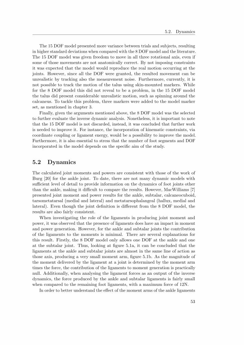
5.2. Dynamics

The 15 DOF model presented more variance between trials and subjects, resultingin higher standard deviations when compared with the 8 DOF model and the literature.The 15 DOF model was given freedom to move in all three rotational axis, even ifsome of those movements are not anatomically correct. By not imposing constraintsit was expected that the model would reproduce the real motion occurring at thejoints. However, since all the DOF were granted, the resulted movement can beunrealistic by tracking also the measurement noise. Furthermore, currently, it isnot possible to track the motion of the talus using skin-mounted markers. Whilefor the 8 DOF model this did not reveal to be a problem, in the 15 DOF modelthe talus did present considerable unrealistic motion, such as spinning around thecalcaneus. To tackle this problem, three markers were added to the model markerset, as mentioned in chapter 3.

Finally, given the arguments mentioned above, the 8 DOF model was the selectedto further evaluate the inverse dynamic analysis. Nonetheless, it is important to notethat the 15 DOF model is not discarded, instead, it was concluded that further workis needed to improve it. For instance, the incorporation of kinematic constraints, viacoordinate coupling or ligament energy, would be a possibility to improve the model.Furthermore, it is also essential to stress that the number of foot segments and DOFincorporated in the model depends on the specific aim of the study.

5.2 Dynamics

The calculated joint moments and powers are consistent with those of the work ofBurg [20] for the ankle joint. To date, there are not many dynamic models withsu�cient level of detail to provide information on the dynamics of foot joints otherthan the ankle, making it di�cult to compare the results. However, MacWilliams [7]presented joint moment and power results for the ankle, subtalar, calcaneocuboid,tarsometatarsal (medial and lateral) and metatarsophalangeal (hallux, medial andlateral). Even though the joint definition is di↵erent from the 8 DOF model, theresults are also fairly consistent.

When investigating the role of the ligaments in producing joint moment andpower, it was observed that the presence of ligaments does have an impact in momentand power generation. However, for the ankle and subtalar joints the contributionof the ligaments to the moments is minimal. There are several explanations forthis result. Firstly, the 8 DOF model only allows one DOF at the ankle and oneat the subtalar joint. Thus, looking at figure 5.1a, it can be concluded that theligaments at the ankle and subtalar joints are almost in the same line of action asthose axis, producing a very small moment arm, figure 5.1b. As the magnitude ofthe moment delivered by the ligament at a joint is determined by the moment armtimes the force, the contribution of the ligaments to moment generation is practicallynull. Additionally, when analysing the ligament forces as an output of the inversedynamics, the force produced by the ankle and subtalar ligaments is fairly smallwhen compared to the remaining foot ligaments, with a maximum force of 12N.

In order to better understand the e↵ect of the moment arms of the ankle ligaments

53

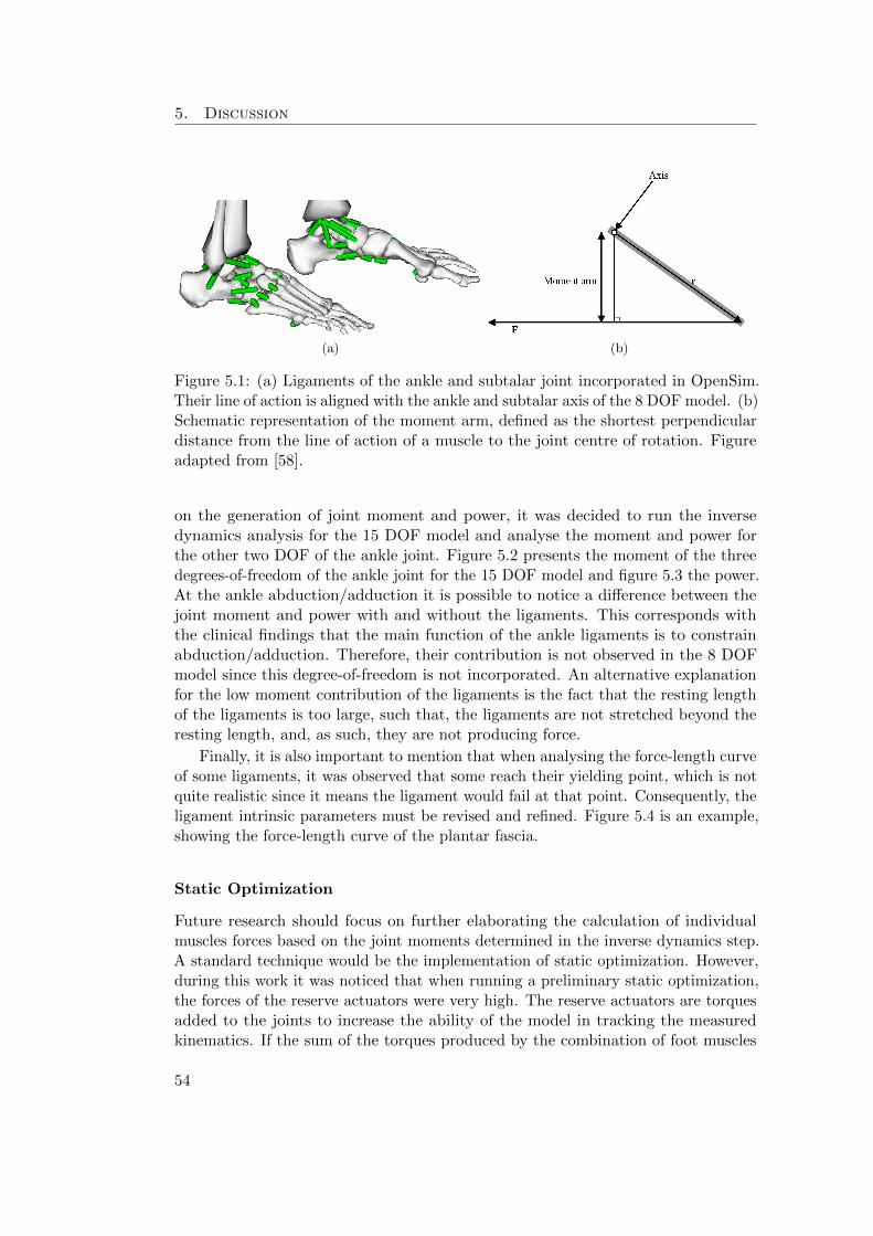
5. Discussion

(a) (b)

Figure 5.1: (a) Ligaments of the ankle and subtalar joint incorporated in OpenSim.Their line of action is aligned with the ankle and subtalar axis of the 8 DOF model. (b)Schematic representation of the moment arm, defined as the shortest perpendiculardistance from the line of action of a muscle to the joint centre of rotation. Figureadapted from [58].

on the generation of joint moment and power, it was decided to run the inversedynamics analysis for the 15 DOF model and analyse the moment and power forthe other two DOF of the ankle joint. Figure 5.2 presents the moment of the threedegrees-of-freedom of the ankle joint for the 15 DOF model and figure 5.3 the power.At the ankle abduction/adduction it is possible to notice a di↵erence between thejoint moment and power with and without the ligaments. This corresponds withthe clinical findings that the main function of the ankle ligaments is to constrainabduction/adduction. Therefore, their contribution is not observed in the 8 DOFmodel since this degree-of-freedom is not incorporated. An alternative explanationfor the low moment contribution of the ligaments is the fact that the resting lengthof the ligaments is too large, such that, the ligaments are not stretched beyond theresting length, and, as such, they are not producing force.

Finally, it is also important to mention that when analysing the force-length curveof some ligaments, it was observed that some reach their yielding point, which is notquite realistic since it means the ligament would fail at that point. Consequently, theligament intrinsic parameters must be revised and refined. Figure 5.4 is an example,showing the force-length curve of the plantar fascia.

Static Optimization

Future research should focus on further elaborating the calculation of individualmuscles forces based on the joint moments determined in the inverse dynamics step.A standard technique would be the implementation of static optimization. However,during this work it was noticed that when running a preliminary static optimization,the forces of the reserve actuators were very high. The reserve actuators are torquesadded to the joints to increase the ability of the model in tracking the measuredkinematics. If the sum of the torques produced by the combination of foot muscles

54

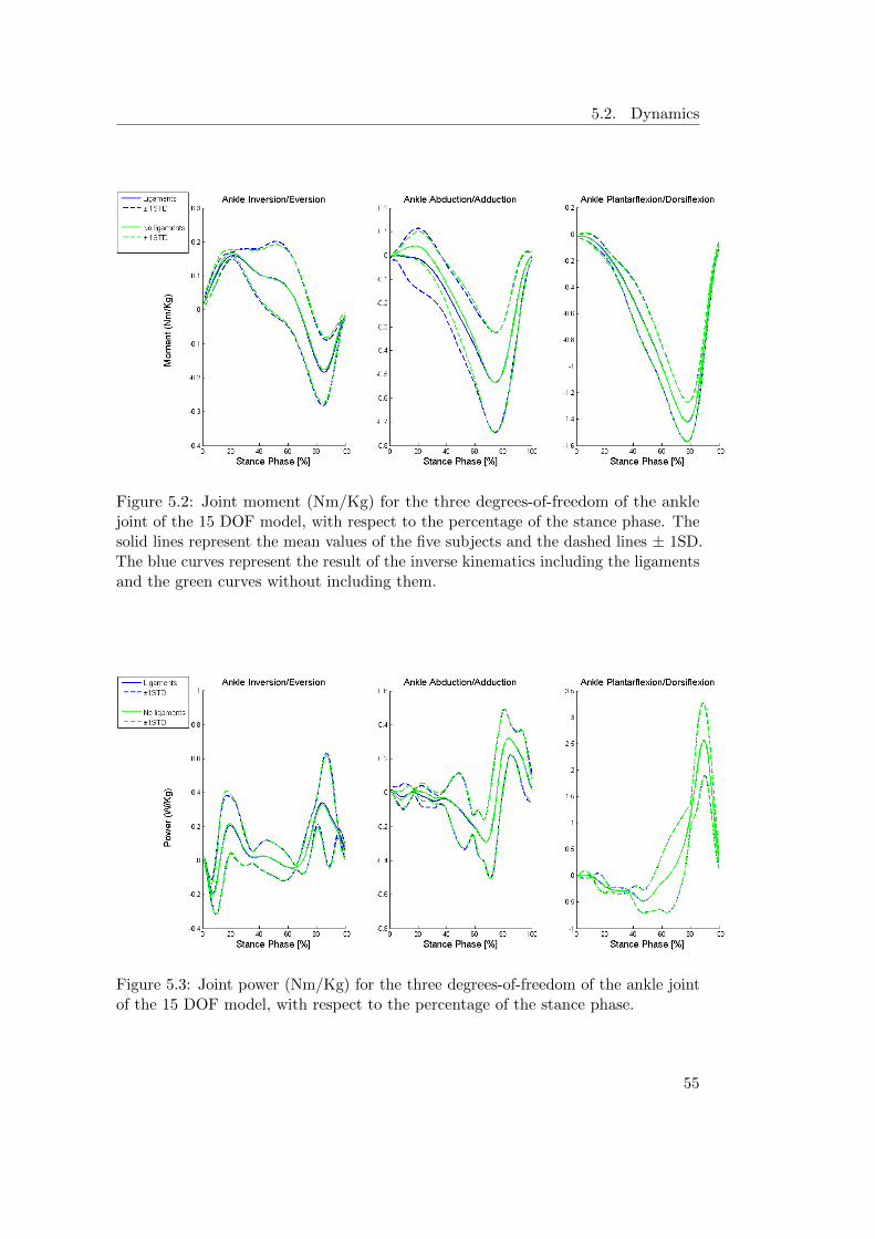
5.2. Dynamics

Figure 5.2: Joint moment (Nm/Kg) for the three degrees-of-freedom of the anklejoint of the 15 DOF model, with respect to the percentage of the stance phase. Thesolid lines represent the mean values of the five subjects and the dashed lines ± 1SD.The blue curves represent the result of the inverse kinematics including the ligamentsand the green curves without including them.

Figure 5.3: Joint power (Nm/Kg) for the three degrees-of-freedom of the ankle jointof the 15 DOF model, with respect to the percentage of the stance phase.

55

5. Discussion

Figure 5.4: Example of the force-length curve of the plantar fascia. The characteristicyield region of the ligament force-length curve was modelled to be constant.

(intrinsic and extrinsic) and ligaments were not able to generate the desired torque, ascalculated via the inverse dynamics, the reserve actuators would be active. As such, itis desired that the contribution of the reserve actuation is minimal. Figures 5.5a and5.5b show that the static optimization cannot find a solution. The solid black line,which represents the result of the inverse dynamics without including the ligaments,should be in between the solid green and red lines, which represent the ligaments’torque plus the minimum and maximum torque of the intrinsic muscles (solid lines)and plus the minimum and maximum torque of both intrinsic and extrinsic muscles(dashed lines). Therefore, since the black lines are not in between the red and greenlines, 5.5a and 5.5b, it is possible to conclude that the static optimization cannotfind a solution. Consequently, it is necessary to first refine the path actuators andligaments’ parameters before proceeding to the static optimization analysis. Theparameter refinement should be done, ideally, based on information collected duringexperimental measurements of the ligament and intrinsic muscles’ characteristics.

56

5.2. Dynamics

(a) (b)

Figure 5.5: (a) Example of the results of the inverse dynamics for the tarsometatarsalfirst ray joint and (b) for the metatarsophalangeal plantarflexion/dorsiflexion joint.The solid black line represents the result of the inverse dynamics without ligaments;the solid blue line is the torque produced by the ligaments; the green lines representthe ligaments’ torque plus the minimum torque of the intrinsic muscles and plus theminimum torque of both intrinsic and extrinsic muscles; the red lines represent theligaments’ torque plus the maximum torque of the intrinsic muscles and plus themaximum torque of both intrinsic and extrinsic muscles.

57

Chapter 6

Conclusion

Modelling the true complexity of the ankle-foot is not yet feasible, however, pro-gressively, it is possible to create fair approximations. In this work, an extendedankle-foot musculoskeletal model was developed in OpenSim, responding to the needfor a more detailed representation of the ankle-foot complex. This was achievedwith the development of two five-segment foot models with 8 and 15 DOF, includingthirty intrinsic muscles and thirty-six ligaments. The models’ performance in termsof kinematics was compared and validated against literature. Moreover, dynamicanalysis were also performed for the 8 DOF model in order to evaluate the jointmoments and power and the ligaments’ contribution. The current developmentsallow to provide more extensive insight in the kinematic and kinetic behaviour ofthe foot in order to aid in the design of customized insoles.

The validation of the foot models proved to be successful as the kinematics andkinetics analysis produced the expected results, according to literature. However,since some experimental trials did not produce optimal results, there are possibleimprovements to be implemented. Firstly, since errors occur during experimental dataacquisition, improving the filtering and treatment of the data is necessary. Secondly,the modelling itself can be improved by, for instance, modelling the translationalmovement of the joints and not only the rotational movement. Thirdly, the markerweight attribution can also be refined, in order to adapt more accurately to eachparticular trial. Furthermore, the development of a new marker protocol to bettermatch the needs of the new five-segment foot model is also a possibility.

When analysing the results of the 8 DOF and 15 DOF model, it was possible toconclude that the 8 DOF model is the most fit for the purpose of this project. Byfollowing the anatomical functionality of the foot, it was able to generate the mostconsistent results across the di↵erent trials and subjects. On the other hand, thekinematics of the 15 DOF showed excessive variability. It is, however, important toemphasize that with the necessary refinements, the 15 DOF model might reveal tobe the most appropriate for a di↵erent study, as the DOF incorporated depend onthe purpose of the model.

Regarding the incorporation of the intrinsic muscles and ligaments, the character-istic parameters that define them need to be refined. The problematic lies on the lack

59

6. Conclusion

of experimental measurements to quantify and characterize these parameters for someof the muscles and ligaments, such as the ligament resting length, nominal sti↵nessor the intrinsic muscles’ contraction velocity. Therefore, the parameters retrievedfrom literature, for some cases, were mere approximations and not experimentallyobtained values. Consequently, as verified when analysing the results, the behaviourof some ligaments (force-length curve) was rather unrealistic. Nonetheless, evaluatingthe contribution of the ligaments to joint moment and power generation, minorcontributions were found at the level of the ankle joint, however a larger e↵ect wasfound at the midfoot and forefoot joints. The calculation of individual muscle forces,the next step of the work-flow, would rely on tuning the parameters of the intrinsicmuscles and ligaments.

Furthermore, future work will also consist on performing forward simulationanalysis in order to verify the model performance in reproducing the plantar pressureprofiles with the use of a contact model.

60

Appendices

61

Appendix A

Intrinsic Muscles

Table A.1 presents the input parameters for modelling the foot intrinsic musclesin OpenSim as Path Actuators. Tables A.2, A.3 and A.4 present their respectivegeometry path.

Table A.1: Parameters of the foot intrinsic muscles.

Muscle Name Isometric Force PCSA

Abductor Hallucis 301.76 6.68Extensor Hallucis Brevis 60.53 1.34Abductor Digiti Minimi 1, 2 and 3 57.07 1.26Lumbrical 2 and 3 18.07 0.4Lumbrical 4 13.55 0.3Lumbrical 5 8.13 0.18Quadratus Plantar Medialis 29.51 0.65Quadratus Plantar Lateralis 15.06 0.33Flexor Digitorum Brevis 2 80.41 1.78Flexor Digitorum Brevis 3 67.31 1.49Flexor Digitorum Brevis 4 56.92 1.26Flexor Digitorum Brevis 5 15.81 0.35Extensor Digitorum Brevis 2 35.69 0.79Extensor Digitorum Brevis 3 23.04 0.51Extensor Digitorum Brevis 4 19.88 0.44Adductor Hallucis Oblique 74.39 1.65Adductor Hallucis Transverse 9.34 0.21Flexor Digiti Minimi Brevis 90.35 2Flexor Hallucis Brevis Medialis 81.31 1.8Flexor Hallucis Brevis Lateralis 95.77 2.12

63

A. Intrinsic Muscles

Table A.2: Geometry path of the intrinsic muscles - part 1.

Muscle Name Point Body Model SegmentAbductor Hallucis Origin Calcaneus Calcaneus

Via Navicular MidfootVia Metatarsal ForefootInsertion ProximalPhalange1 Toes

Extensor Hallucis Brevis Origin Calcaneus CalcaneusVia Intermediate Cuneiform MidfootVia Metatarsal1 ForefootInsertion ProximalPhalange Toes

Abductor Digiti Minimi1 Origin Calcaneus CalcaneusVia Metatarsal5 ForefootVia Metatarsal5 ForefootInsertion ProximalPhalange5 Toes



Lumbrical2 Origin FlexorDigitorumLongusTendon MidfootVia Metatarsal2 ForefootInsertion ProximalPhalange2 Toes




Quadratus Plantar Medialis1 Origin Calcaneus CalcaneusInsertion FlexorDigitorumLongusTendon Midfoot

64


Muscle Name Point Body Model SegmentQuadratus Plantar Medialis2 Origin Calcaneus Calcaneus

Insertion FlexorDigitorumLongusTendon Midfoot

Quadratus Plantar Medialis3 Origin Calcaneus CalcaneusInsertion FlexorDigitorumLongusTendon Midfoot

Quadratus Plantar Lateralis1 Origin Calcaneus CalcaneusInsertion FlexorDigitorumLongusTendon Midfoot



Flexor Digitorum Brevis2 Origin Calcaneus CalcaneusVia Cuboid MidfootVia Metatarsal2 ForefootVia ProximalPhalange2 ToesInsertion MiddlePhalange2 Toes



Flexor Digitorum Brevis5 Origin Calcaneus CalcaneusVia Cuboid MidfootVia Metatarsal5 ForefootInsertion MiddlePhalange5 Toes

Extensor Digitorum Brevis2 Origin Calcaneus CalcaneusVia Metatarsal3 ForefootVia Metatarsal2 ForefootVia Metatarsal2 Forefoot

65

A. Intrinsic Muscles


Muscle Name Point Body Model SegmentExtensor Digitorum Brevis3 Origin Calcaneus Calcaneus

Via Metatarsal3 ForefootVia Metatarsal3 ForefootVia Metatarsal3 Forefoot

Extensor Digitorum Brevis4 Origin Calcaneus CalcaneusVia Metatarsal4 ForefootVia Metatarsal4 Forefoot

Adductor Hallucis Oblique1 Origin Metatarsal2 ForefootVia Metatarsal1 ForefootInsertion Proximal Phalange1 Toes



Adductor Hallucis Transverse1 Origin Metatarsal3 ForefootVia Metatarsal1 ForefootInsertion Proximal Phalange1 Toes

Adductor Hallucis Transverse2 Origin Metatarsal4 ForefootVia Metatarsal1 ForefootInsertion Proximal Phalange1 Toes

Flexor Digiti Minimi Brevis Origin Metatarsal5 ForefootVia Metatarsal5 ForefootInsertion Proximal Phalange5 Toes

Flexor Hallucis Brevis Medialis Origin Navicular MidfootVia Metatarsal1 ForefootVia Metatarsal1 ForefootInsertion Proximal Phalange1 Toes

Flexor Hallucis Brevis Lateralis Origin Navicular MidfootVia Metatarsal1 ForefootVia Metatarsal1 ForefootInsertion Proximal Phalange1 Toes

66

Appendix B

Ligaments

Table B.1 presents the input parameters for modelling the foot ligaments in OpenSim.Tables B.2, B.3, B.4 and B.5 present their respective geometry path.

67

B. Ligaments

Table B.1: Parameters of the foot ligaments.

Ligament Resting Nominal Nominal Relative Initial Relative sti↵ness NominalName Length Strain Force Stifness at nominal strain Stifness

L0 (m) " F (N) k

init

k

nom

k (N/m)TibioTalarPost 0.023 0.125 39.14 0.25 3.8 13855.14TibioTalarAnt 0.029 0.125 19.56 0.26 2.85 5415.48TibioCalcaneal 0.034 0.083 18.97 0.2 4.1 6648.50TibioNavicular 0.047 0.125 450.00 1 1 77374.76TaloFibularPost 0.034 0.083 4.53 0.14 4.15 1590.75TaloFibularAnt 0.034 0.175 47.53 0.3 2.51 7895.51CalcaneoFibular 0.041 0.083 10.12 0.1 3.8 2995.20PlantarFascia1Ph 0.163 0.036 62.74 0.6 1.5 10694.89PlantarFascia2Ph 0.164 0.036 62.74 0.6 1.5 10609.67PlantarFascia3Ph 0.163 0.036 50.19 0.6 1.5 8528.85PlantarFascia4Ph 0.155 0.036 37.64 0.6 1.5 6736.18PlantarFascia5Ph 0.146 0.036 37.64 0.6 1.5 7155.45LongPlantar1 0.092 1.000 5383.13 1 1 58730.56LongPlantar2 0.087 1.000 4037.34 1 1 46185.92LongPlantar3 0.082 1.000 2691.56 1 1 32996.03LongPlantar4 0.073 1.000 1345.78 1 1 18472.40CalcaneoNavicularPlantar1 0.022 1.000 1032.85 1 1 46019.95CalcaneoNavicularPlantar2 0.014 1.000 1200.00 1 1 86692.61CalcaneoNavicularPlantar3 0.012 1.000 1200.00 1 1 101095.88CalcaneoCuboidPlantar1 0.020 1.000 1500.00 1 1 74419.53CalcaneoCuboidPlantar2 0.026 1.000 1500.00 1 1 57284.57CalcaneoCuboidDorsal 0.029 1.000 1032.85 1 1 35615.38TaloNavicularDorsal1 0.013 1.000 500.00 1 1 37683.63TaloNavicularDorsal2 0.013 1.000 500.00 1 1 37683.60CalcaneoNavicularBifurcate 0.019 1.000 1032.85 1 1 54608.87CalcaneoCuboidBifurcate 0.016 1.000 1032.85 1 1 63712.04TarsoMetatarsalDorsal1 0.014 1.000 500.00 1 1 34498.41TarsoMetatarsalDorsal3 0.011 1.000 500.00 1 1 45524.49TarsoMetatarsalDorsal5 0.008 1.000 200.00 1 1 25625.19TarsoMetatarsalDorsal7 0.010 1.000 500.00 1 1 51428.32TarsoMetatarsalDorsal8 0.008 1.000 500.00 1 1 59842.86TarsoMetatarsalPlantar1 0.010 1.000 1032.00 1 1 100199.82TarsoMetatarsalPlantar2 0.008 1.000 20913.46 1 1 2462555.57TarsoMetatarsalPlantar3 0.008 1.000 20913.46 1 1 2629730.45TarsoMetatarsalPlantar4 0.009 1.000 500.00 1 1 57175.35TarsoMetatarsalPlantar5 0.010 1.000 500.00 1 1 48895.98

68

Table B.2: Ligaments’ geometry path - part 1.

Ligament Point Body Model Segment

TibioTalarPost Origin Tibia TibiaInsertion Talus Talus

TibioTalarAnt Origin Tibia TibiaInsertion Talus Talus

TibioCalcaneal Origin Tibia TibiaInsertion Calcaneus Calcaneus

TibioNavicular Origin Tibia TibiaInsertion Navicular Midfoot

TaloFibularPost Origin Tibia TibiaInsertion Talus Talus

TaloFibularAnt Origin Tibia TibiaInsertion Talus Talus

CalcaneoFibular Origin Tibia TibiaInsertion Calcaneus Calcaneus

PlantarFascia1Ph Origin Calcaneus CalcaneusVia Metatarsal1 ForefootInsertion ProximalPhalange1 Toes



69

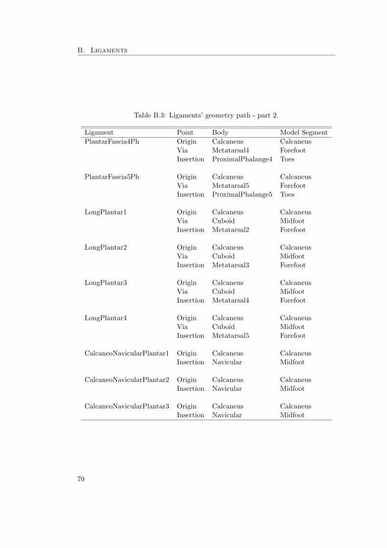
B. Ligaments


Ligament Point Body Model SegmentPlantarFascia4Ph Origin Calcaneus Calcaneus

Via Metatarsal4 ForefootInsertion ProximalPhalange4 Toes


LongPlantar1 Origin Calcaneus CalcaneusVia Cuboid MidfootInsertion Metatarsal2 Forefoot




CalcaneoNavicularPlantar1 Origin Calcaneus CalcaneusInsertion Navicular Midfoot



70


Ligament Point Body Model SegmentCalcaneoCuboidPlantar1 Origin Calcaneus Calcaneus

Insertion Cuboid Midfoot

CalcaneoCuboidPlantar2 Origin Calcaneus CalcaneusInsertion Cuboid Midfoot

CalcaneoCuboidDorsal Origin Calcaneus CalcaneusInsertion Cuboid Midfoot

TaloNavicularDorsal1 Origin Talus TalusInsertion Navicular Midfoot

TaloNavicularDorsal2 Origin Talus TalusInsertion Navicular Midfoot

CalcaneoNavicularBifurcate Origin Calcaneus CalcaneusInsertion Navicular Midfoot

CalcaneoCuboidBifurcate Origin Calcaneus CalcaneusInsertion Cuboid Midfoot

TarsoMetatarsalDorsal1 Origin Medial Cuneiform MidfootInsertion Metatarsal1 Forefoot

TarsoMetatarsalDorsal3 Origin Intermediate Cuneiform MidfootInsertion Metatarsal2 Forefoot

71

B. Ligaments


Ligament Point Body Model SegmentTarsoMetatarsalDorsal5 Origin Lateral Cuneiform Midfoot

Insertion Metatarsal3 Forefoot

TarsoMetatarsalDorsal7 Origin Cuboid MidfootInsertion Metatarsal4 Forefoot

TarsoMetatarsalDorsal8 Origin Cuboid MidfootInsertion Metatarsal5 Forefoot

TarsoMetatarsalPlantar1 Origin Medial Cuneiform MidfootInsertion Metatarsal1 Forefoot

TarsoMetatarsalPlantar2 Origin Intermediate Cuneiform MidfootInsertion Metatarsal2 Forefoot

TarsoMetatarsalPlantar3 Origin Lateral Cuneiform MidfootInsertion Metatarsal3 Forefoot

TarsoMetatarsalPlantar4 Origin Cuboid MidfootInsertion Metatarsal4 Forefoot

TarsoMetatarsalPlantar5 Origin Cuboid MidfootInsertion Metatarsal5 Forefoot

72

Appendix C

Abstract: CMBBE 2015

The abstract of the publication to be presented in the thirteenth InternationalSymposium on Computer Methods in Biomechanics and Biomedical Engineering2015 (CMBBE).

73

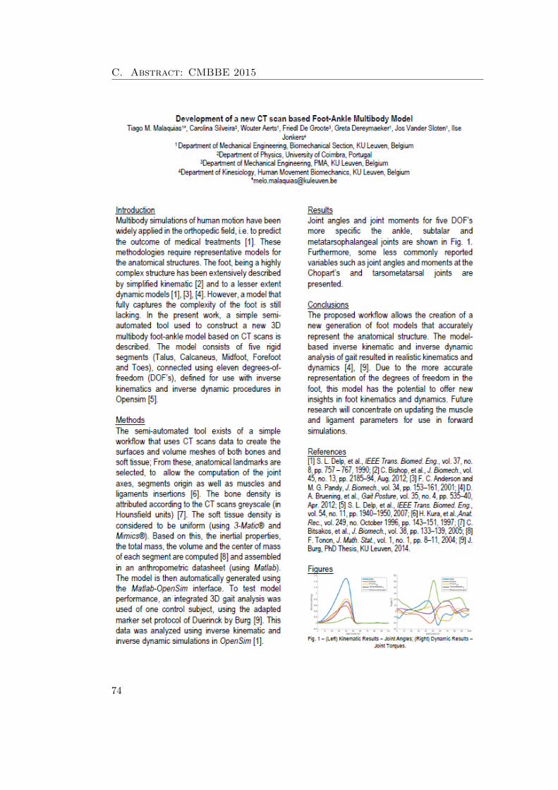
C. Abstract: CMBBE 2015

74

Bibliography

[1] D. A. Winter. Biomechanics and motor control of human movement. 1990.

[2] Rosa Pamies Vila. Application of Multibody Dynamics Techniques To TheAnalysis of Human Gait. PhD thesis, Universitat Politecnica de Catalunya,2012.

[3] E Muybridge. Animal locomotion. An electro-photographic investigation ofconsecutive phases of animal movements. Photogravure company of New York,University of Pennsylvania, New York, 1887.

[4] Simtk.org. OpenSim Project Overview. https://simtk.org/home/opensim.Date of access: 2015-05-22.

[5] Steven M Kidder, Faruk S Abuzzahab, Gerald F Harris, and Je↵rey E Johnson.A System for the Analysis of Foot and Ankle Kinematics During Gait. EEETransactions on Rehabilitation Engineering, 4(1), 1996.

[6] Sylvain Carbes, Sø ren Tø rholm, Scott Telfer, Jim Woodburn, Michiel Oost-erwaal, and John Rasmussen. A new multisegmental foot model and markerprotocol for accurate simulation of the foot biomechanics during walking. Pro-ceedings of ISB 2011 Congress XXIII, pages 1–2, 2011.

[7] Bruce A. MacWilliams, Matthew Cowley, and Diane E. Nicholson. Foot kine-matics and kinetics during adolescent gait. Gait and Posture, 17(3):214–224,2003.

[8] J. Stebbins, M. Harrington, N. Thompson, a. Zavatsky, and T. Theologis.Repeatability of a model for measuring multi-segment foot kinematics in children.Gait and Posture, 23(4):401–410, 2006.

[9] H. Cenk Guler, Necip Berme, and Sheldon R. Simon. A viscoelastic spheremodel for the representation of plantar soft tissue during simulations. Journalof Biomechanics, 31(9):847–853, 1998.

[10] Nori Okita, Steven a. Meyers, John H. Challis, and Neil a. Sharkey. An objectiveevaluation of a segmented foot model. Gait and Posture, 30(1):27–34, 2009.

[11] J. H. Hicks. The mechanics of the foot. Journal of anatomy, 88(Pt 1):25–30.1,1954.

75

https://simtk.org/home/opensim

Bibliography

[12] Michael Whittle. Gait Analysis: An Introduction. Butterworth-Heinemann,2007.

[13] Richard D. Lannotti, Joseph P.; Parker. The Netter collection of medicalillustrations. 6: The musculoskeletal system Part 2: Spine and lower limb.Philadelphia Elsevier Saunders, 2013.

[14] Henry Gray. Classification of Joints. In Anatomy of the Human Body, pages1821–1865. 1918.

[15] C. H. Barnett and J. R. Napier. The axis of rotation at the ankle joint in man.J. Anat. London, (86):1–9, 1952.

[16] Shahan K. Sarrafian. Anatomy of the Foot and Ankle. Descriptive, Topographic,Functional. J. B. Lippincott Company, 1983.

[17] Yi-Chung Lin, Hyung Joo Kim, and Marcus G. Pandy. A computationallye�cient method for assessing muscle funtion during human locomotion. Interna-tional Journal for Numerical Methods in Biomedical Engineering, 27(1):436–449,2011.

[18] Hideji Kura, Zong Ping Luo, Harold B. Kitaoka, and Kai Nan An. Quantitativeanalysis of the intrinsic muscles of the foot. Anatomical Record, 249(1):143–151,1997.

[19] Pau Golano, Jordi Vega, Peter a J de Leeuw, Francesc Malagelada, M. CristinaManzanares, Vıctor Gotzens, and C. Niek van Dijk. Anatomy of the ankleligaments: A pictorial essay. Knee Surgery, Sports Traumatology, Arthroscopy,18(5):557–569, 2010.

[20] Josefien Burg. Biomechanics of the foot-ankle complex before and after totalankle arthroplasty : An in vivo and in vitro analysis. PhD thesis, KU Leuven,2014.

[21] M. C. Carson, M. E. Harrington, N. Thompson, J. J. O’Connor, and T. N.Theologis. Kinematic analysis of a multi-segment foot model for researchand clinical applications: A repeatability analysis. Journal of Biomechanics,34(10):1299–1307, 2001.

[22] Uangthip Rattanaprasert, Richard Smith, Martin Sullivan, and Wendy Gilleard.Three-dimensional kinematics of the forefoot, rearfoot, and leg without thefunction of tibialis posterior in comparison with normals during stance phase ofwalking. Clinical Biomechanics, 14(1):14–23, 1999.

[23] Stephen C. Cobb, Laurie L. Tis, Je↵rey T. Johnson, Yong Tai Wang, Mark D.Geil, and Frances a. McCarty. The e↵ect of low-mobile foot posture on multi-segment medial foot model gait kinematics. Gait and Posture, 30(3):334–339,2009.

76

Bibliography

[24] Zimi Sawacha, Giuseppe Cristoferi, Gabriella Guarneri, Stefano Corazza, GiuliaDona, Paolo Denti, Andrea Facchinetti, Angelo Avogaro, and Claudio Cobelli.Characterizing multisegment foot kinematics during gait in diabetic foot patients.Journal of Neuroengineering and Rehabilitation, 6:37, 2009.

[25] Josh Tome, Deborah a Nawoczenski, Adolph Flemister, and Je↵ Houck. Compari-son of foot kinematics between subjects with posterior tibialis tendon dysfunctionand healthy controls. The Journal of Orthopaedic and Sports Physical therapy,36(9):635–644, 2006.

[26] A. Leardini, M. G. Benedetti, L. Berti, D. Bettinelli, R. Nativo, and S. Giannini.Rear-foot, mid-foot and fore-foot motion during the stance phase of gait. Gaitand Posture, 25(3):453–462, 2007.

[27] Paolo Caravaggi, Claudia Giacomozzi, and Alberto Leardini. Foot segmentsmobility and plantar pressure in the normal foot. Journal of Foot and AnkleResearch, 7(Suppl 1):A11, 2014.

[28] Ryan Maha↵ey, Stewart C Morrison, Wendy I Drechsler, and Mary C Cramp.Evaluation of multi-segmental kinematic modelling in the paediatric foot usingthree concurrent foot models. Journal of foot and ankle research, 6(1):43, 2013.

[29] Stephen H. Scott and David a. Winter. Biomechanical model of the humanfoot: Kinematics and kinetics during the stance phase of walking. Journal ofBiomechanics, 26(9):1091–1104, 1993.

[30] F.S. Abuzzahab, G.F. Harris, S.M. Kidder, and J.E. Johnson. A kinetic, biome-chanical model of the foot and ankle. Proceedings of 16th Annual InternationalConference of the IEEE Engineering in Medicine and Biology Society, pages 0–1,1994.

[31] Dustin a. Bruening, Kevin M. Cooney, and Frank L. Buczek. Analysis of akinetic multi-segment foot model part II: Kinetics and clinical implications. Gaitand Posture, 35(4):535–540, 2012.

[32] S. L. Delp, J. P. Loan, and M. G. Hoy. An interactive graphics-based model ofthe lower extremity to study orthopedic surgical procedures. IEEE transactionson Biomedical Engineering, 37(8):757–767, 1990.

[33] R. R. Neptune, I. C. Wright, and a. J. Van Den Bogert. A Method for NumericalSimulation of Single Limb Ground Contact Events: Application to Heel-ToeRunning. Computer Methods in Biomechanics and Biomedical Engineering,3(4):321–334, 2000.

[34] F C Anderson and M G Pandy. Dynamic optimization of human walking.Journal of biomechanical engineering, 123(5):381–390, 2001.

77

Bibliography

[35] AnyScript Community. The Glasgow-Maastricht Foot Model (FootGM), 2013.http://wiki.anyscript.org/index.php/AnyBody_Body_Model. Date of ac-cess: 2015-03-22.

[36] Scott L. Delp, Frank C. Anderson, Allison S. Arnold, Peter Loan, AymanHabib, Chand T. John, Eran Guendelman, and Darryl G. Thelen. OpenSim:Open-source software to create and analyze dynamic simulations of movement.IEEE Transactions on Biomedical Engineering, 54(11):1940–1950, 2007.

[37] Cindy; Au and James Dunne. Gait 2392 and 2354 Models,2013. http://simtk-confluence.stanford.edu:8080/display/OpenSim/

Gait+2392+and+2354+Models. Date of access: 2015-06-26.

[38] Carl Gans. Fiber architecture and muscle function. Exercise & Sport ScienceReviews, 10(1):160–207, 1982.

[39] Da Winter. Biomechanics and motor control of human gait: normal, elderlyand pathological. 1991.

[40] P. Provenzano, R. Lakes, T. Keenan, and R. Vanderby. Nonlinear ligamentviscoelasticity. Annals of Biomedical Engineering, 29(10):908–914, 2001.

[41] A Viidik. Simultaneous mechanical and light microscopic studies of collagenfibers. Z Anat Entwicklungsgesch., 136(2):204–12, 1972.

[42] Albert L. Kwansa, Yvonne M. Empson, Emmanuel C. Ekwueme, Valerie I.Walters, Joseph W. Freeman, and Cato T. Laurencin. Novel matrix basedanterior cruciate ligament (ACL) regeneration. Soft Matter, 6(20):5016, 2010.

[43] A/S AnyBody Technology. Anybody Tutorials - Lesson7: Ligaments.http://www.anybodytech.com/fileadmin/AnyBody/Docs/Tutorials/

chap5_Muscle_modeling/lesson7.html. Date of access: 2015-03-06.

[44] J R Funk, G W Hall, J R Crandall, and W D Pilkey. Linear and quasi-linear viscoelastic characterization of ankle ligaments. Journal of biomechanicalengineering, 122(1):15–22, 2000.

[45] Bernard Mengiardi, Marco Zanetti, Philip B Schottle, Patrick Vienne, BeataBode, Juerg Hodler, and Christian W a Pfirrmann. Spring ligament complex: MRimaging-anatomic correlation and findings in asymptomatic subjects. Radiology,237(1):242–249, 2005.

[46] Clarissa Canella Moraes Do Carmo, Lina Isabel Fonseca De Almeida Melao,Marcio Freitas Valle De Lemos Weber, Debra Trudell, and Donald Resnick.Anatomical features of plantar aponeurosis: Cadaveric study using ultrasonog-raphy and magnetic resonance imaging. Skeletal Radiology, 37(10):929–935,2008.

78

Bibliography

[47] Vishwas Patil, Nabil a Ebraheim, Alexandra Frogameni, and Jiayong Liu.Morphometric dimensions of the calcaneonavicular (spring) ligament. Foot &ankle international / American Orthopaedic Foot and Ankle Society [and] SwissFoot and Ankle Society, 28(8):927–932, 2007.

[48] John Rule. Pictorial Essay Spring Ligament of the Ankle : Normal MR Anatomy.American Journal of Roentgenology, 161(6):1241–1244, 1993.

[49] Rita Stagni, Alberto Leardini, and Andrea Ensini. Ligament fibre recruitmentat the human ankle joint complex in passive flexion. Journal of Biomechanics,37(12):1823–1829, 2004.

[50] Jennifer Hicks. Marker (.trc) Files, 2013. http://simtk-confluence.

stanford.edu:8080/display/OpenSim/Marker+%28.trc%29+Files. Date ofaccess: 2015-06-26.

[51] Jennifer Hicks. How Scaling Works, 2015. http://simtk-confluence.

stanford.edu:8080/display/OpenSim/How+Scaling+Works. Date of access:2015-06-26.

[52] Christopher Hicks, Jennifer; Dembia. How to use the scale tool,2013. http://simtk-confluence.stanford.edu:8080/display/OpenSim/

How+to+Use+the+Scale+Tool. Date of access: 2015-06-26.

[53] F. De Groote, T. De Laet, I. Jonkers, and J. De Schutter. Kalman smoothingimproves the estimation of joint kinematics and kinetics in marker-based humangait analysis. Journal of Biomechanics, 41(16):3390–3398, 2008.

[54] Christopher Hicks, Jennifer; Dembia. How Inverse Kinematics Works,2013. http://simtk-confluence.stanford.edu:8080/display/OpenSim/

How+Inverse+Kinematics+Works. Date of access: 2015-06-28.

[55] Jennifer Lund, Katherine; Hicks. Getting Started with Inverse Dynamics,2012. http://simtk-confluence.stanford.edu:8080/display/OpenSim/

Getting+Started+with+Inverse+Dynamics. Date of access: 2015-06-29.

[56] Jennifer Hicks. How Inverse Dynamics Works, 2012. http://simtk-confluence.stanford.edu:8080/display/OpenSim/How+Inverse+Dynamics+Works. Dateof access: 2015-06-29.

[57] P. Lundgren, C. Nester, a. Liu, a. Arndt, R. Jones, a. Staco↵, P. Wolf, anda. Lundberg. Invasive in vivo measurement of rear-, mid- and forefoot motionduring walking. Gait and Posture, 28(1):93–100, 2008.

[58] Wikipedia. Torque. https://en.wikipedia.org/wiki/Torque. Date of access:2015-07-06.

79

extended'biomechanical'model'of'the' … carolina... ·...

Documents