extending integral concepts to curved bridge systems
TRANSCRIPT
University of Nebraska - Lincoln University of Nebraska - Lincoln
DigitalCommons@University of Nebraska - Lincoln DigitalCommons@University of Nebraska - Lincoln
Civil Engineering Theses, Dissertations, and Student Research Civil Engineering
11-2011
Extending Integral Concepts to Curved Bridge Systems Extending Integral Concepts to Curved Bridge Systems
Saeed Eghtedar Doust University of Nebraska-Lincoln, [email protected]
Follow this and additional works at: https://digitalcommons.unl.edu/civilengdiss
Part of the Civil Engineering Commons, and the Structural Engineering Commons
Eghtedar Doust, Saeed, "Extending Integral Concepts to Curved Bridge Systems" (2011). Civil Engineering Theses, Dissertations, and Student Research. 41. https://digitalcommons.unl.edu/civilengdiss/41
This Article is brought to you for free and open access by the Civil Engineering at DigitalCommons@University of Nebraska - Lincoln. It has been accepted for inclusion in Civil Engineering Theses, Dissertations, and Student Research by an authorized administrator of DigitalCommons@University of Nebraska - Lincoln.
EXTENDING INTEGRAL CONCEPTS TO CURVED BRIDGE SYSTEMS
by
Saeed Eghtedar Doust
A DISSERTATION
Presented to the Faculty of
The Graduate College at the University of Nebraska
In Partial Fulfillment of Requirements
For the Degree of Doctor of Philosophy
Major: Interdepartmental Area of Engineering
(Civil Engineering)
Under the Supervision of Professors Elizabeth G. Jones and Atorod Azizinamini
Lincoln, Nebraska
November, 2011

EXTENDING INTEGRAL CONCEPTS TO CURVED BRIDGE SYSTEMS Saeed Eghtedar Doust, Ph.D.
University of Nebraska, 2011
Advisors: Elizabeth Jones and Atorod Azizinamini
The behavior of integral abutment systems and the extension of their application to curved bridges are investigated. First, the stresses in the elements of a typical integral abutment are studied by conducting nonlinear finite element analysis using the software package Abaqus. The results are design recommendations for the details of such abutments. The effect of integral abutments on the responses of bridges is also investigated. Steel and concrete bridge systems are studied separately.
The studied steel bridge systems are composed of composite I-girder superstructures and integral abutments supported on steel H-piles. A series of finite element studies for different bridge lengths and radii are conducted and the effects of several load cases on the bridges are studied. In these bridges, the stresses in the abutment piles are of critical importance from the design standpoint. The results show that horizontal curvature mitigates these stresses. The bridge movement is also studied and a procedure to find the end displacements of curved bridges is presented. Pile orientation is another significant design factor that is studied elaborately. The results indicate that, for straight bridges, the strong-axis pile bending yields lower levels of stress. A method for finding the optimum pile orientation in curved integral bridges is developed. The effect of different bearing types is also investigated. This investigation reveals the superior structural performance of elastomeric bearings compared to other bearing types.
The concrete bridge systems that are studied consist of voided slab superstructures, integral abutments and concrete drilled shafts. A matrix of finite element studies is performed for different lengths and curvatures. Similar to steel I-girder bridges, it is concluded that horizontal curvature mitigates the internal forces of the abutment elements. The orientation of the concrete shafts is also examined which again shows the advantage of strong-axis orientation. Integral abutment bridges can have flexible piers integrally connected to the superstructure to eliminate all the bridge bearings. The effect of such integral piers on the internal forces of integral abutments is also examined. In these flexible piers, moment magnification can be of crucial significance. It is shown that choosing the integral abutment system reduces the magnification effects in the slender pier columns compared to jointed bridge systems.

ii
© Copyright by
Saeed E. Doust
(2011)

iii
Dedication
To
My wife Golboo
and
My daughter Taraneh

iv
Acknowledgement
The present dissertation was conducted in the National Bridge Research Organization
under the supervision of Professor Atorod Azizinamini. I am really thankful of him for
his guidance, advice and help throughout the course of my doctoral studies.
I would like to express my sincere thanks to Professor Andrezj Nowak for his valuable
considerations during the past years. His attention has meant a lot to me. I am extremely
appreciative of his continual kindness.
I am deeply grateful of Professor Mehrdad Negahban for his valuable guidance and
friendship. He gave me confidence in the most difficult days that I had.
I wish to thank Professor Elizabeth Jones, the Graduate Chair of the department for
her sincere helps and guidance. I also thank Professor Fred Choobineh who served on my
committee and evaluated my studies. And I appreciate the friendship and assistance of
Dr. Aaron Yakel during the past years. I will never forget his precious helps.
I want to offer my special thanks to my beloved wife, Golboo, for her priceless
patience, understanding and support. If she was not helping me, I was not able to
accomplish this work. I owe her a life. And I apologize my daughter, Taraneh, for those
times that I was tired and couldn’t play with her. I promise to spend more time for her
from now on.
At the end, I would like to thank my parents for spending their lives on my growth and
progress.

v
Table of Contents
Table of Contents .......................................................................................... v
List of Figures… ........................................................................................... xi
List of Tables….. ........................................................................................ xix
Chapter 1 Introduction, Background and Objectives ........................ 1 1.1 Introduction .......................................................................................................... 1
1.2 Background ........................................................................................................... 6
1.3 Literature Review ................................................................................................. 7 1.3.1 Straight IA Bridges .......................................................................................... 8 1.3.2 Curved Bridges .............................................................................................. 10
A) Analysis..................................................................................................... 14 B) Elastic lateral torsional buckling capacity ................................................ 15 C) Cross-Frame Spacing ................................................................................ 16 D) Effect of Cross Frames .............................................................................. 16 E) Flange Local Buckling of Curved Girders ................................................ 17
1.3.3 Curved IA Bridges ......................................................................................... 17
1.4 Scope .................................................................................................................. 19
1.5 Objectives of the study ....................................................................................... 20
Chapter 2 Mechanistic Study of Curved IAB ................................... 23 2.1 Introduction ........................................................................................................ 23
2.2 Analysis of a Curved Girder ............................................................................... 24
2.3 Analysis of an I-Girder under Torsion ............................................................... 27
2.4 Analysis of Two-girder Bridges ......................................................................... 32
2.5 Analysis of Multi-girder Bridges ........................................................................ 37
2.6 Cross Frame Spacing .......................................................................................... 41
Chapter 3 Detailed Study of Connections in an Integral Abutment 43 3.1 Introduction ........................................................................................................ 43
3.2 Abutment Configuration ..................................................................................... 44
3.3 Steel Material Modeling ..................................................................................... 45 3.3.1 Tension Test ................................................................................................... 48 3.3.2 Validity of Constant Volume Assumption .................................................... 52

vi
3.3.3 Elastic Rebound of Cross Section .................................................................. 54 3.3.4 Proposing a New Model for Steel Material ................................................... 56 3.3.5 Curve Fitting .................................................................................................. 57 3.3.6 A Sample Model: Grade 50 Steel .................................................................. 61
3.4 Concrete Material Modeling ............................................................................... 61 3.4.1 Concrete Response under Compression ........................................................ 62 3.4.2 Concrete Compression Response Models ..................................................... 63
A) Hognestad Model ...................................................................................... 64 B) Polynomial Model ..................................................................................... 65 C) Carreira and Chu Model............................................................................ 65 D) Comparison of Different Models .............................................................. 66
3.4.3 Concrete Response under Tension ................................................................. 67 3.4.4 Concrete Tension Response Models .............................................................. 68 3.4.5 Concrete Response Modeling in Abaqus ....................................................... 72 3.4.6 Employed Concrete Models .......................................................................... 77
3.5 Elements ............................................................................................................. 79 3.5.1 C3D8(R) ........................................................................................................ 79 3.5.2 C3D4 .............................................................................................................. 81 3.5.3 C3D10M ........................................................................................................ 81 3.5.4 T3D2 .............................................................................................................. 81
3.6 Stress Functions Definition ................................................................................ 81
3.7 Finite Element Modeling .................................................................................... 85
3.8 Moment Capacity of the Superstructure ............................................................. 98
3.9 Results of Analysis ........................................................................................... 101 3.9.1 Girder Stresses ............................................................................................. 101
A) Effect of Girder Stiffener ........................................................................ 102 B) Effect of Girder End Shear Studs............................................................ 103 C) Ultimate Loading .................................................................................... 104
3.9.2 Abutment Wall Stresses At Girder Embedment Zone ................................. 108 A) Effect of Girder Stiffener on Wall Stresses ............................................ 109 B) Effect of Girder End Shear Studs............................................................ 110
3.9.3 Abutment Wall Stresses At Pile Embedment Zone ..................................... 112 A) Effect of Pile Stiffener ............................................................................ 113
3.9.4 Pile Stresses ................................................................................................. 114 A) Effect of Pile Stiffener ............................................................................ 115
Chapter 4 Effect of Curvature on Steel IA Bridges ........................ 117 4.1 Introduction ...................................................................................................... 117
4.2 Bridge Configuration ........................................................................................ 118 4.2.1 Superstructure .............................................................................................. 118 4.2.2 Abutments .................................................................................................... 120 4.2.3 Piers ............................................................................................................. 121
4.3 Finite Element Modeling .................................................................................. 123

vii
4.3.1 Material Properties ....................................................................................... 123 4.3.2 Loading ........................................................................................................ 124
A) Dead Load (DC) ...................................................................................... 124 B) Wearing Surface Load (DW) .................................................................. 124 C) Earth Pressure (EH) ................................................................................ 125 D) Live Load (LL) ....................................................................................... 126 E) Braking Force (BR)................................................................................. 127 F) Centrifugal Force (CE) ........................................................................... 128 G) Wind Load (WS) ..................................................................................... 129 H) Uniform Temperature Changes (TU) ...................................................... 133 I) Temperature Gradient (TG) .................................................................... 133 J) Shrinkage (SH)........................................................................................ 134
4.3.3 Load Combinations ...................................................................................... 138 4.3.4 Soil-Structure Interaction ............................................................................. 140
A) Soil-Abutment interaction ....................................................................... 141 B) Soil-Pile Interaction ................................................................................ 143 B1) Lateral Load‐Deflection in Soft Clay ................................................................ 144
B2) Lateral Load‐Deflection in Sand ....................................................................... 147
4.3.5 Elements ...................................................................................................... 152 A) Beam Element ......................................................................................... 153 B) Shell Element .......................................................................................... 153 C) Nonlinear Link Element .......................................................................... 154 D) Nonlinear Support Element ..................................................................... 157
4.3.6 Finite Element Models ................................................................................. 158
4.4 Results of FE Analysis ..................................................................................... 159 4.4.1 Effects of Length and Curvature on Load Responses ................................. 161
A) Bending Moment of Abutment Piles ...................................................... 163 A1) Contraction ...................................................................................................... 164
A2) Expansion ......................................................................................................... 166
A3) Live Load .......................................................................................................... 168
A4) Wind Load ........................................................................................................ 170
A5) Dead Load ........................................................................................................ 172
A6) Concrete Shrinkage.......................................................................................... 174
A7) Horizontal Earth Pressure ................................................................................ 176
A8) Centrifugal Force ............................................................................................. 178
A9) Weight of Wearing Surface ............................................................................. 179
A10) Braking Force ................................................................................................... 181
A11) Positive Temperature Gradient ....................................................................... 183
A12) Negative Temperature Gradient ..................................................................... 185

viii
A13) Combination of the Loads ............................................................................... 186
B) Shear Force of Abutment Piles ............................................................... 188 4.4.2 Bridge Movement ........................................................................................ 189
A) Factors Affecting Bridge Displacement .................................................. 192 B) Bridge Shortening Due to Contraction ................................................... 196 C) Bridge Shortening Due to Shrinkage ...................................................... 198 D) Total Bridge Shortening .......................................................................... 199 E) Effect of Bridge Width on the Displacement Direction .......................... 201 E1) Effect of Width on Contraction End Displacement ......................................... 201
E2) Effect of width on Shrinkage End Displacement ............................................. 202
E3) Effect of width on Total End Displacement ..................................................... 202
F) Direction of Displacement ...................................................................... 204 G) Bridge End Displacement ....................................................................... 207 H) Step by Step Procedure ........................................................................... 211 I) Example .................................................................................................. 212
4.4.3 Pile Orientation ............................................................................................ 214 A) Analysis of Modeled Bridges with Weak and Strong Orientation for Abutment Piles .................................................................................................... 217 B) The Procedure to Find the Optimal Pile Orientation .............................. 228
4.4.4 Effect of Bearing Type and Orientation ...................................................... 228 A) Effect of Bearing Type on Abutment Pile Moments .............................. 230 B) Effect of Bearing Type on Pier Columns Moments ................................ 231 C) Bearing Orientation ................................................................................. 234
Chapter 5 Effect of Curvature on Concrete IA Bridges ................. 237 5.1 Introduction ...................................................................................................... 237
5.2 Bridge Configuration ........................................................................................ 238 5.2.1 Superstructure .............................................................................................. 238 5.2.2 Abutments .................................................................................................... 239 5.2.3 Piers ............................................................................................................. 240
5.3 Finite Element Modeling .................................................................................. 242 5.3.1 Material Properties ....................................................................................... 242 5.3.2 Loading ........................................................................................................ 242
A) Dead Load (DC) ...................................................................................... 243 B) Wearing Surface Load (DW) .................................................................. 243 C) Earth Pressure (EH) ................................................................................ 244 D) Live Load (LL) ....................................................................................... 244 E) Braking Force (BR)................................................................................. 246 F) Centrifugal Force (CE) ........................................................................... 246 G) Uniform Temperature Changes ............................................................... 247 H) Temperature Gradient ............................................................................. 248 I) Shrinkage ................................................................................................ 248
5.3.3 Soil-Structure Interaction ............................................................................. 250

ix
A) Soil-Abutment Interaction ...................................................................... 250 B) Soil-Pile Interaction ................................................................................ 251 B1) Lateral Load‐Deflection in Soft Clay ................................................................ 251
B2) Lateral Load‐Deflection in Sand ....................................................................... 254
5.3.4 Elements ...................................................................................................... 257 A) Beam Element ......................................................................................... 258 B) Shell Element .......................................................................................... 258 C) Nonlinear Link Element .......................................................................... 258 D) Nonlinear Support Element ..................................................................... 260
5.3.5 Finite Element Models ................................................................................. 261
5.4 Results of FE Analysis ..................................................................................... 262 5.4.1 Effect of Length and curvature on Load Responses .................................... 263
A) Bending Moment of Abutment Piles ...................................................... 263 A1) Contraction ...................................................................................................... 263
A2) Expansion ......................................................................................................... 264
A3) Live Load .......................................................................................................... 265
A4) Dead Load ........................................................................................................ 266
A5) Concrete Shrinkage.......................................................................................... 267
A6) Horizontal Earth Pressure (EH) ........................................................................ 268
A7) Centrifugal Force ............................................................................................. 271
A8) Weight of Wearing Surface ............................................................................. 272
A9) Braking Force ................................................................................................... 273
A10) Positive Temperature Gradient ....................................................................... 274
A11) Negative Temperature Gradient ..................................................................... 275
A12) Combination of the Loads ............................................................................... 276
B) Shear Forces of Abutment Piles .............................................................. 277 5.4.2 Pile Orientation ............................................................................................ 277 5.4.3 Bearing-Isolated Pier vs. Flexible Integral Pier ........................................... 284 5.4.4 Mitigation of Moment Magnification .......................................................... 285
Chapter 6 Concluding Remarks and Future Research .................. 291 6.1 Connections of Integral Abutments .................................................................. 291
6.2 Steel I-girder IA Bridges .................................................................................. 292 6.2.1 Effects of Bridge length and curvature on load responses .......................... 293 6.2.2 Bridge Movement ........................................................................................ 295 6.2.3 Pile Orientation ............................................................................................ 297 6.2.4 Effect of Bearing Type ................................................................................ 297
6.3 Concrete IA Bridges ......................................................................................... 299

x
6.3.1 Effects of Bridge Length and Curvature on Load Responses ...................... 299 6.3.2 Pile Orientation ............................................................................................ 301 6.3.3 Bearing-Isolated Piers versus Integral Piers ................................................ 302 6.3.4 Mitigation of Moment Magnification Factor ............................................... 302
6.4 Recommendations for Future Research ............................................................ 303
References 305
Appendix A Effect of Bridge Length and Curvature on Shear Force of Abutment Piles 317
A1 Contraction ....................................................................................................... 317
A2 Expansion ......................................................................................................... 319
A3 Live Load .......................................................................................................... 321
A4 Wind Load ........................................................................................................ 323
A5 Dead Load ........................................................................................................ 325
A6 Concrete Shrinkage .......................................................................................... 327
A7 Horizontal Earth Pressure ................................................................................. 329
A8 Centrifugal Force .............................................................................................. 331
A9 Weight of Wearing Surface .............................................................................. 332
A10 Braking Force ................................................................................................... 334
A11 Positive Temperature Gradient ......................................................................... 336
A12 Negative Temperature Gradient ....................................................................... 337
A13 Combination of the Loads ................................................................................ 339
Appendix B MATLAB Moment-curvature Program ................. 342-351

xi
List of Figures
Figure 1.1-1 A Typical a) Integral Abutment b) Semi-Integral Abutment .................... 4
Figure 2.2-1 Plan View of a Curved Girder Under Gravity Loads in z Direction .......... 24
Figure 2.3-1 Effect of Torsional Moment Applied to a Cantilever I-Girder (Boresi et al.) ...........................................................................................................
28
Figure 2.4-1 Plan View of the Two-Girder Bridge ........................................................ 33
Figure 2.4-2 Flange Forces of the Girders ...................................................................... 33
Figure 2.4-3 Equilibrium of a Segment of the Girder Flange ........................................ 34
Figure 2.4-4 3D View of the Two-Girder Bridge ........................................................... 35
Figure 2.5-1 Cross Section of the Multi-Girder Curved Bridge ..................................... 37
Figure 3.2-1 General Configuration of an Integral Abutment ........................................ 45
Figure 3.3-1 Strain-Stress Curves (Tension Test # 1) .................................................... 49
Figure 3.3-2 Strain-Stress Curves (Tension Test # 2) .................................................... 50
Figure 3.3-3 Strain-Stress Curves (Tension Test # 3) .................................................... 50
Figure 3.3-4 Strain-Stress Curves (Tension Test # 4) .................................................... 51
Figure 3.3-5 Designation of the Key Points on the Strain-Stress Curves ....................... 56
Figure 3.3-6 Scheme of Fitted Curve Between Points C and D ..................................... 59
Figure 3.3-7 Fitted Curve Between Points C and D ....................................................... 60
Figure 3.3-8 Material Model for Grade 50 Steel ............................................................ 61
Figure 3.4-1 Strain-Stress Curves of Concrete Specimens of Different Strength .......... 63
Figure 3.4-2 Hognestad Model for Strain-Stress of Concrete in Compression ............. 64
Figure 3.4-3 Strain-Stress Curves of Concrete in Compression in Different Models .... 67
Figure 3.4-4 Strain-Stress Curves of Concrete in Tension in Different Models ............ 68
Figure 3.4-5 Schematic Strain-Stress Curve of Concrete in Tension ............................. 69
Figure 3.4-6 Strain-Stress Curves of Concrete in Tension and Compression ................ 73
Figure 3.4-7 Biaxial Failure Surface of Concrete ........................................................... 75
xii
Figure 3.4-8 Definition of Compressive Inelastic strain Used for Definition of Compression Hardening Data (Abaqus Documentation) ...........................
76
Figure 3.4-9 Definition of Tensile Cracking Strain used for Definition of Tension Stiffening Data ...........................................................................................
77
Figure 3.4-10 Total and Inelastic Strain vs. Stress for 4 ksi Concrete in Compression ... 78
Figure 3.4-11 Total and Cracking Strain vs. Stress for 4 ksi Concrete in Tension .......... 79
Figure 3.5-1 C3D8 Brick Element .................................................................................. 80
Figure 3.5-2 C3D10M Tetrahedron Element .................................................................. 81
Figure 3.7-1 General Configuration of the Integral Abutment Model ............................ 86
Figure 3.7-2 Girder Element of the Connection ............................................................. 87
Figure 3.7-3 Embedded End of the Girder...................................................................... 88
Figure 3.7-4 Highlighted Position of the Girder Element............................................... 89
Figure 3.7-5 Concrete Wall of the Abutment ................................................................. 90
Figure 3.7-6 Highlighted Position of the Abutment Wall............................................... 91
Figure 3.7-7 Highlighted Position of the Deck Slab ....................................................... 92
Figure 3.7-8 Haunch Element of the Connection ........................................................... 92
Figure 3.7-9 Highlighted Position of the Haunch ........................................................... 93
Figure 3.7-10 H- Pile Element of the Connection ............................................................ 94
Figure 3.7-11 Highlighted Position of the H-Piles ........................................................... 95
Figure 3.7-12 Highlighted Rebars of the Deck Slab ......................................................... 96
Figure 3.7-13 Highlighted Rebars of the Abutment Wall ................................................ 97
Figure 3.7-14 Shear Studs Attached to the Girder Bottom Flange ................................... 97
Figure 3.8-1 Superstructure Section at the Vicinity of Abutment Wall (Section A-A) ...............................................................................................................
99
Figure 3.8-2 Moment–Curvature of the Superstructure at Section A-A ......................... 99
Figure 3.8-3 Stress Distribution in the Superstructure at the Vicinity of Abutment Wall Corresponding to Maximum Moment Capacity ................................
100
Figure 3.9-1 Mises Stresses of Girder without any Stiffener or End Shear Stud ........... 102
Figure 3.9-2 Mises Stresses of Girder with Stiffener without End Shear Stud .............. 103
Figure 3.9-3 Mises Stresses of Girder with End Shear Stud without Stiffener .............. 104
Figure 3.9-4 Mises Stresses of Half of the Girder .......................................................... 105
Figure 3.9-5 Mises Stresses of Concrete Deck ............................................................... 106
Figure 3.9-6 Mises Stresses of Girder’s End Corresponding to Mid-span Plastification ...............................................................................................
107

xiii
Figure 3.9-7 Mises Stresses of Abutment Wall Supporting an Unstiffened Girder ...... 108
Figure 3.9-8 Mises Stresses of Abutment Wall Supporting a Stiffened Girder.............. 109
Figure 3.9-9 Mises Stresses of Abutment Wall - Girder without End Shear Studs ........ 111
Figure 3.9-10 Mises Stresses of Abutment Wall - Girder with End Shear Studs ............. 111
Figure 3.9-11 Mises Stresses of the Concrete Wall Around the Piles .............................. 112
Figure 3.9-12 Stiffened Pile at the Wall Lower Face Section .......................................... 113
Figure 3.9-13 Mises Stresses of the Concrete Wall Around the Piles with Stiffener ....... 114
Figure 3.9-14 Mises Stresses of Abutment Piles .............................................................. 115
Figure 3.9-15 Mises Stresses of Abutment Piles with Stiffener ....................................... 116
Figure 4.1-1 A Curved Steel I-girder Bridge Similar to the Studied Bridges ................ 118
Figure 4.2-1 Cross Section of the Composite Steel Superstructure ................................ 119
Figure 4.2-2 Steel I-Girder Dimensions ......................................................................... 120
Figure 4.2-3 Abutment Integral Details .......................................................................... 121
Figure 4.2-4 Pier Configuration ...................................................................................... 122
Figure 4.2-5 Springs Modeling the Bearings of the Piers ............................................... 123
Figure 4.3-1 Wearing Surface of the Modeled Steel Bridges ......................................... 125
Figure 4.3-2 Positioning of the Live Load ...................................................................... 127
Figure 4.3-3 Positive Temperature Gradient in the Superstructure Section ................... 134
Figure 4.3-4 Annual Average Ambient Relative Humidity in Percent ........................... 136
Figure 4.3-5 Relationship of Wall Movement vs. Soil Pressure..................................... 142
Figure 4.3-6 Force-Displacement Curves of the Abutment Backfill Springs ................. 143
Figure 4.3-7 Force-Displacement Curves of the Springs of Piles of Abutments in Soft Clay ....................................................................................................
146
Figure 4.3-8 Force-Displacement Curves of the Springs of Piles of Piers in Soft Clay ............................................................................................................
147
Figure 4.3-9 Initial Modulus of Subgrade Reaction ....................................................... 148
Figure 4.3-10 Values of Coefficients , and as a Function of Angle of Friction .......................................................................................................
150
Figure 4.3-11 Force-Displacement Curves of the Springs of Piles of Piers in Sand ........ 151
Figure 4.3-12 Force-Displacement Curves of the Springs of Piles of Abutments in Sand ............................................................................................................
152
Figure 4.3-13 Modeling of the Bearings ........................................................................... 156
Figure 4.3-14 Typical Finite Element Models of the Studied Bridges ............................. 159

xiv
Figure 4.4-1 Maximum Moment in Abutment Piles Due to Contraction ....................... 165
Figure 4.4-2 Normalized Moment in Abutment Piles Due to Contraction ..................... 166
Figure 4.4-3 Maximum Moment in Abutment Piles Due to Expansion ......................... 167
Figure 4.4-4 Normalized Moment in Abutment Piles Due to Expansion ....................... 168
Figure 4.4-5 Maximum Moment in Abutment Piles Due to Live Load ......................... 169
Figure 4.4-6 Normalized Moment in Abutment Piles Due to Live Load ....................... 170
Figure 4.4-7 Maximum Moment in Abutment Piles Due to Wind Load ........................ 171
Figure 4.4-8 Normalized Moment in Abutment Piles Due to Wind Load...................... 172
Figure 4.4-9 Maximum Moment in Abutment Piles Due to Dead Load ........................ 173
Figure 4.4-10 Normalized Moment in Abutment Piles Due to Dead Load ...................... 174
Figure 4.4-11 Maximum Moment in Abutment Piles Due to Concrete Shrinkage .......... 175
Figure 4.4-12 Normalized Moment in Abutment Piles Due to Concrete Shrinkage ........ 176
Figure 4.4-13 Maximum Moment in Abutment Piles Due to Horizontal Earth Pressure ......................................................................................................
177
Figure 4.4-14 Normalized Moment in Abutment Piles Due to Horizontal Earth Pressure ......................................................................................................
178
Figure 4.4-15 Maximum Moment in Abutment Piles Due to Centrifugal Force.............. 179
Figure 4.4-16 Maximum Moment in Abutment Piles Due to Weight of wearing Surface .......................................................................................................
180
Figure 4.4-17 Normalized Moment in Abutment Piles Due to Weight of Wearing Surface .......................................................................................................
181
Figure 4.4-18 Maximum Moment in Abutment Piles Due to Braking Force ................... 182
Figure 4.4-19 Normalized Moment in Abutment Piles Due to Braking Force ................. 183
Figure 4.4-20 Maximum Moment in Abutment Piles Due to Positive Temperature Gradient ......................................................................................................
184
Figure 4.4-21 Normalized Moment in Abutment Piles Due to Positive Temperature Gradient ......................................................................................................
184
Figure 4.4-22 Maximum Moment in Abutment Piles Due to Negative Temperature Gradient ......................................................................................................
185
Figure 4.4-23 Normalized Moment in Abutment Piles Due to Negative Temperature Gradient ......................................................................................................
186
Figure 4.4-24 Maximum Moment in Abutment Piles in Load Combinations Envelope .. 187
Figure 4.4-25 Normalized Moment in Abutment Piles in Load Combinations Envelope .....................................................................................................
188
Figure 4.4-26 Directions of End Displacements in A Curved Bridge .............................. 193

xv
Figure 4.4-27 Bridge End Movement- a) Pure Translation -b) Rotation .......................... 194
Figure 4.4-28 Modification Factor for Bridge Shortening Due to Contraction ................ 197
Figure 4.4-29 Modification Factor for Bridge Shortening Due to Shrinkage................... 199
Figure 4.4-30 Modification Factor for Bridge Shortening Applied to Total Shortening ..................................................................................................
200
Figure 4.4-31 Direction of End Displacement Due to Contraction .................................. 201
Figure 4.4-32 Angles and in Total Displacement .............................................. 203
Figure 4.4-33 Values / ° versus W/Lc ...................................................................... 204
Figure 4.4-34 Modified Displacement Directions versus L/R .......................................... 207
Figure 4.4-35 Deformed Bridge General Configuration ................................................... 208
Figure 4.4-36 Deformed Bridge Simplified Configuration .............................................. 209
Figure 4.4-37 Critical Load Combination Type ............................................................... 215
Figure 4.4-38 Critical Load Combination Type ............................................................... 223
Figure 4.4-39 Direction of Pile Displacement .................................................................. 224
Figure 4.4-40 Average Displacement Directions of Abutment Piles Top Node .............. 225
Figure 4.4-41 Design Displacement Directions of Abutment Piles Top Node ................ 226
Figure 4.4-42 Bending Moment of Abutment Piles with Different Bearing Types ......... 230
Figure 4.4-43 Longitudinal Bending Moment of Pier Columns with Different Bearing Types ............................................................................................
232
Figure 4.4-44 Transverse Bending Moment of Pier Columns with Different Bearing Types ..........................................................................................................
234
Figure 4.4-45 Guided Bearing Orientation in Jointed Bridges ......................................... 235
Figure 4.4-46 Guided Bearing Orientation in Bridges with Restraint Superstructure for a Trial Point ..........................................................................................
236
Figure 5.1-1 A Concrete Curved Integral Bridge Similar to the Studied Bridges .......... 238
Figure 5.2-1 Cross Section of the Superstructure of the Modeled Bridges .................... 239
Figure 5.2-2 A Typical Integral Connection for Voided Slab Bridges ........................... 240
Figure 5.2-3 Integral Connection of Piers and Superstructure ....................................... 241
Figure 5.2-4 Bearing-Isolated Connection of Piers and Superstructure ......................... 241
Figure 5.3-1 Wearing Surface of the Modeled Bridges .................................................. 244
Figure 5.3-2 Positioning of the Live Load (distances in inch) ....................................... 245
Figure 5.3-3 Force-Displacement Curves of the Abutment Backfill Springs ................. 251
Figure 5.3-4 Force-Displacement Curves of the Springs of Piles of Abutments in Soft Clay ....................................................................................................
253

xvi
Figure 5.3-5 Force-Displacement Curves of the Springs of Piles of Piers in Soft Clay ............................................................................................................
254
Figure 5.3-6 Force-Displacement Curves of the Springs of Piles of Piers in Sand ........ 256
Figure 5.3-7 Force-Displacement Curves of the Springs of Piles of Abutments in Sand ............................................................................................................
257
Figure 5.3-8 Modeling of the Elastomeric Bearings ....................................................... 260
Figure 5.3-9 A Typical Finite Element Model of the Studied Bridges ........................... 262
Figure 5.4-1 Maximum Moment of Abutment Piles Due to Contraction ....................... 264
Figure 5.4-2 Maximum Moment of Abutment Piles Due to Expansion ......................... 265
Figure 5.4-3 Maximum Moment of Abutment Piles Due to Live Load ......................... 266
Figure 5.4-4 Maximum Moment of Abutment Piles Due to Dead Load ........................ 267
Figure 5.4-5 Maximum Moment of Abutment Piles Due to Concrete Shrinkage .......... 268
Figure 5.4-6 Maximum Moment of Abutment Piles Due to Horizontal Earth Pressure ......................................................................................................
269
Figure 5.4-7 Plan View of Deformed Shape of the Bridge with R=200’ under EH ....... 270
Figure 5.4-8 Plan View of Deformed Shape of the Bridge with R=600’ under EH ....... 270
Figure 5.4-9 Plan View of Deformed Shape of the Bridge with R=1000’ under EH ..... 271
Figure 5.4-10 Maximum Moment of Abutment Piles Due to Centrifugal Force ............. 272
Figure 5.4-11 Maximum Moment of Abutment Piles Due to Weight of Wearing Surface .......................................................................................................
273
Figure 5.4-12 Maximum Moment of Abutment Piles Due to Braking Force ................... 274
Figure 5.4-13 Maximum Moment of Abutment Piles Due to Positive Temperature Gradient ......................................................................................................
275
Figure 5.4-14 Maximum Moment of Abutment Piles Due to Negative Temperature Gradient ......................................................................................................
276
Figure 5.4-15 Envelope of Moment of Abutment Piles in Different Load Combinations .............................................................................................
277
Figure 5.4-16 PCACOL Design Sheet for Strong-Axis Orientation (1 of 2) ................... 280
Figure 5.4-17 PCACOL Design Sheet for Strong-Axis Orientation (2 of 2) ................... 281
Figure 5.4-18 PCACOL Design Sheet for Weak-Axis Orientation (1 of 2) ..................... 282
Figure 5.4-19 PCACOL Design Sheet for Weak-Axis Orientation (2 of 2) ..................... 283
Figure 5.4-20 Envelope of Moment of Abutment Piles in Different Load Combinations in Bridges with Integral Piers vs. Bridges with Elastomeric Isolated Piers ..........................................................................
285
Figure 5.4-21 ∆ Effect in Non-Sway Mode ................................................................... 288

xvii
Figure 5.4-22 ∆ Effect in Sway Mode ........................................................................... 288
Figure 5.4-23 ∆ Effect in a Jointed Abutment Bridge with Flexible Piers .................... 289
Figure 5.4-24 ∆ Effect in an Integral Abutment Bridge with Flexible Piers ................. 290
Figure A-1. Maximum Shear Force in Abutment Piles Due to Contraction ................. 318
Figure A-2. Normalized Shear Force in Abutment Piles Due to Contraction ............... 319
Figure A-3. Maximum Shear Force in Abutment Piles Due to Expansion ................... 320
Figure A-4. Normalized Shear Force in Abutment Piles Due to Expansion ................. 321
Figure A-5. Maximum Shear Force in Abutment Piles Due to Live Load .................... 322
Figure A-6. Normalized Shear Force in Abutment Piles Due to Live Load ................. 323
Figure A-7. Maximum Shear Force in Abutment Piles Due to Wind Load .................. 324
Figure A-8. Normalized Shear Force in Abutment Piles Due to Wind Load ................ 325
Figure A-9. Maximum Shear Force in Abutment Piles Due to Dead Load................... 326
Figure A-10. Normalized Shear Force in Abutment Piles Due to Dead Load ................ 327
Figure A-11. Maximum Shear Force in Abutment Piles Due to Concrete Shrinkage..... 328
Figure A-12. Normalized Shear Force in Abutment Piles Due to Concrete Shrinkage .. 329
Figure A-13. Maximum Shear Force in Abutment Piles Due to Earth Pressure ............. 330
Figure A-14. Normalized Shear Force in Abutment Piles Due to Earth Pressure ........... 331
Figure A-15. Maximum Shear Force in Abutment Piles Due to Centrifugal Force ........ 332
Figure A-16. Maximum Shear Force in Abutment Piles Due to Weight of Wearing Surface .......................................................................................................
333
Figure A-17. Normalized Shear Force in Abutment Piles Due to Weight of Wearing Surface .......................................................................................................
334
Figure A-18. Maximum Shear Force in Abutment Piles Due to Braking Force ............. 335
Figure A-19. Normalized Shear Force in Abutment Piles Due to Braking Force ........... 335
Figure A-20. Maximum Shear Force in Abutment Piles Due to Positive Temperature Gradient ......................................................................................................
336
Figure A-21. Normalized Shear Force in Abutment Piles Due to Positive Temperature Gradient ................................................................................
337
Figure A-22. Maximum Shear Force in Abutment Piles Due to Negative Temperature Gradient ................................................................................
338
Figure A-23. Normalized Shear Force in Abutment Piles Due to Negative Temperature Gradient ................................................................................
339
Figure A-24. Envelope of Maximum Shear Force in Abutment Piles in Different Load Combinations ....................................................................................
340

xviii
Figure A-25.
Envelope of Normalized Shear Force in Abutment Piles in Different Load Combinations ....................................................................................
341

xix
List of Tables
Table 1.1-1 Different Types of Jointless Bridges .......................................................... 3
Table 2.5-1 C Factor for Different Number of Girders ................................................. 40
Table 4.3-1 Multilane Presence Factors ........................................................................ 126
Table 4.3-2 C Factor for Different Radii ....................................................................... 129
Table 4.3-3 Base Wind Pressure, Corresponding to .................... 130
Table 4.3-4 Values of and for Various Upstream Conditions ............................ 131
Table 4.3-5 Base Wind Pressure, for Various Angles of Attack ............................. 131
Table 4.3-6 Wind Pressure, for Various Angles of Attack ...................................... 133
Table 4.3-7 Proposed API p-y Curve for Soft Clay ...................................................... 144
Table 4.4-1 Normalized Weight Factors for Bending Moment of Abutment Piles ...... 163
Table 4.4-2 Direction of Total Displacement (Results of FE Analyses) (W=60’-8”) ... 202
Table 4.4-3 Angles and Modified Angles of Total Displacement Direction ................. 206
Table 4.4-4 Ratios of Abutment Pile Stresses (Weak Axis Orientation to Strong Axis Orientation) ........................................................................................
219
Table 4.4-5 Critical Load Combination Category for Abutment Pile Stresses ............. 222
Table 4.4-6 Ratio of Piles Weak-axis Orientation Stress to Optimized Stress ............. 227
Table 4.4-7 Ratio of Piles Strong-axis Orientation Stress to Optimized Stress ............ 227
Table 4.4-8 Different Bearing Types and the Associated DOF’s.................................. 229
Table 5.3-1 C Factor for Different Radii ....................................................................... 247
Table 5.4-1 Internal Forces of Shafts with Different Orientations ................................ 278

Chapter 1
Introduction, Background
and Objectives
1.1 Introduction
Bridges have been built since thousands of years ago by human beings. From
prehistoric times to the Renaissance bridges had two main characteristics: The main
construction materials were stone and natural cement and the spans were less than 100
feet. Despite the limitations that the architects and engineers of those times had, long
bridges up to a total length of 1000 feet can be found among ancient bridges. After the
Renaissance, modern bridges came into existence in the seventeen and eighteen century.
The greatest differences of these modern bridges and the old ones were the material and
span length. The material changed to iron (or steel) and later concrete. The span length
gradually increased up to 3000 feet in the early twentieth century. So, the engineers were
in charge of designing longer and longer bridges.
This trend in building bridges caused new approaches to appear in bridge industry. To
accommodate the movements of long bridges, the designers adopted new techniques in

2
their designs. Moveable expansion joints and bearings were among those techniques.
These devices have been used in bridges for more than 200 years. But, their performance
has affected the long term performance of new bridges. Expansion joints have different
designs which all of them have some sort of dysfunction. Even though they have high
quality in the first months or years of service, after a longer time, most of them have
problems such as leakage and poor ride quality due to wear or fracture. Bearings also
have shown their intrinsic problems. In most bearing types, elastomeric layers are used.
These elastomers lose their original properties in time. Ozone can damage the elastomer,
even if there is no load or movement applied to the elastomer. That’s why most of
bearings should be replaced after some years.
The deficiencies of expansion joints and bearings drew the bridge designers to some
new concepts of bridge design in the past years. Elimination of joints and bearings was
the new target. This led to the introduction of a new type of structural system known as
Integral bridges. These bridges are composed of:
- Abutments at the two ends
- Approach slabs that rest on abutments and their backfill
- Intermediate piers
- And finally a “jointless” superstructures built integral to the abutments
Note that there are no joints from the end to end of approach slabs. This bridge system
is an ideal one which has no bearings and no joints. But, based on the needs, some other
structural systems have also developed. First is an integral bridge that has rigid piers with
movable and/or fixed bearings. In this type of bridges, all expansion joints and also the

3
abutment bearings are eliminated. But, piers still have bearings. If the durability of the
pier bearings is guaranteed, these bridges can survive for a long time without any major
deterioration. The second system has integral piers, but it has bearings in the abutments.
In these bridges, the piers are flexible to be able to accommodate the movements, and the
abutments are rigid, so they are isolated from the superstructure. A third system is a
jointless bridge that has bearings both in the abutments and piers. Those jointless
structural systems that have bearings in the abutments are called semi-integral. Table 1.1-
1 shows different types of jointless bridges.
Bridge Type Joint Bearing
over Piers
Bearing in
Abutments
Integral with Flexible Piers No No No
Integral with Rigid Piers No Yes No
Semi-integral with Flexible Piers No No Yes
Semi-integral with Rigid Piers No Yes Yes
Table 1.1-1. Different Types of Jointless Bridges
As described before, integral bridges do not have joints whether they have bearings or
not. Therefore, a better name for these bridges is “Jointless”. These two terms have been
used interchangeably in the literature and also in the present study. The integral bridges
with no bearing in the abutments are sometimes called “integral Abutment Bridges”.
Figure 1.1-1 illustrates typical integral and semi-integral abutment details.

4
Figure 1.1-1. A Typical a) Integral Abutment b) Semi-Integral Abutment
Integral bridges have several advantages compared to jointed ones. The main
advantages include:
- Lower initial and maintenance cost
- Longer service life
- No water leakage from superstructure down to substructure
- Improved riding quality
- Easier and faster construction
- Easier inspection
- More resistant to pavement growth/pressure phenomenon
- Reduced number of bearings (except for semi-integral with rigid piers)
- Easier embankment compaction
Span
Girder
Span
a) b)
Girder
ElastomericBearing

5
- No need to cofferdams for abutment excavation and pile driving
- Small excavation for abutments
- No need to battered piles for flexible abutments or piers
- Increased factor of safety for buoyancy
- Simple formwork for abutments and piers pile caps
- Fewer joints (just two joints at the ends of approach slabs)
- Broader construction tolerance
- Reduced removal of existing substructure (new configuration to straddle old
foundations)
- Simple beam seat details
- Elimination of bearing anchor bars
- Broader end to intermediate span ratio
- No risk of superstructure falling during major earthquakes and eliminating seat
width requirements in seismic design
- More distribution for live load
- Simpler Design (if the bending stiffness of abutment piles is ignored)
In the present study, both types of integral abutment bridges, with flexible and rigid
piers, are studied. The abbreviations used for these bridges depending on the context are
IA for “integral abutment” and IAB for “integral abutment bridges”.

6
1.2 Background
The first integral abutment bridge in the United States was built in 1938. Since then
building integral bridges has spread throughout the country. Construction of integral
bridges has also been adopted in Europe, Australia, New Zealand, Japan, South Korea
and some other countries.
In the first decades, integral bridge systems were used for bridges with concrete
superstructure. These bridges had a length between 50 to 100 feet. It was not until early
1960’s that this concept was adopted for steel girder bridges. After that, several steel
bridges with a skew angle less than 30 degrees and lengths not more than 300 feet were
constructed using this method. Jointless steel bridges of length less than 300 feet have
had an excellent performance in some states like North Dakota, South Dakota and
Tennessee. Such bridges with concrete superstructures have been constructed and served
with lengths of less than 800 feet in other states like California, Kansas and Colorado.
In 1987, eleven states of the US reported construction of jointless integral bridges with
lengths of about 300 feet. Among those states, Tennessee and Missouri implemented the
approach to longer bridges. Missouri reported concrete and steel integral bridges with the
length of 500 and 600 feet, respectively. Tennessee DOT is leading the way in
construction of long integral bridges. They have constructed a prestressed concrete
integral abutment bridge with a length of 1175 feet.
The same tendency is seen in other countries. In Europe, European Commission is
spreading the integral bridge concept among bridge designers. In the UK, integral and
semi-integral bridge systems are recommended for relatively short bridges with less than
7
30 degrees skew angle. In Canada, integral construction is encouraged among designers
where each province has its own provisions for these bridges. Ontario recommends
jointless technique for bridges shorter than 328 feet.
The above mentioned trend shows that making use of integral bridges will become
standard among the bridge designers and responsible agencies like DOT’s in the near
future. But, the use of this type of bridges becomes even more popular when
comprehensive design guides are available and if their enhanced long term performance
and durability is more proven. On the other hand, as thousand of existing bridges are
jointed and during years are deteriorated, converting them into jointless integral bridges
appears to be a reasonable solution if the design provisions and details of such bridges are
documented. That will ensure the designers and owners of their decision and there will be
more justification for adoption of such methodology.
1.3 Literature Review
To have a detailed study on curved integral abutment bridges, three different subjects
should be considered: curved bridges, integral bridges and curved integral bridges. This is
attributed to the fact that the problems associated with a curved jointed bridge or a
straight integral bridge may be inherited by a curved integral bridge. Therefore, the
literature review on curved integral abutment bridges is carried out in three steps. First,
the previous research on integral abutment straight bridges is reviewed. These studies
mainly include the investigations on thermal response and examination of the available
field monitoring data related to integral bridges. Then, the studies that have been
conducted on curved bridges are examined. This part presents a summary of decades of

8
research on the behavior of curved I- and box-girder bridges, their design requirements
and the approaches to evaluate their strength. And then, the previous studies on curve
integral abutment bridges are briefly summarized.
1.3.1 Straight IA Bridges
Straight integral bridges have been the subject of several studies. National Steel
Bridge Alliance of American Iron and Steel Institute has published a report on integral
abutments for steel bridges (American Iron and Steel Institute, Tennessee, Dept. of
Transportation, Structures Division, & National Steel Bridge Alliance, 1996). This report
authored by Wasserman and Walker was one of the first ones discussing the details and
basic design requirements of steel integral bridges. As an almost old report, it has been a
conservative guideline for designing integral bridges. The report discusses the practices
of design agencies, the geometrical and construction limitations of jointless bridges and
also provides an elementary example for design of piles.
Arsoy et al. have prepared a report for Virginia Transportation Research Council that
presents the results of their works in a literature review, field trip and a finite element
analysis related to integral bridges (Arsoy et al., 1999). They have concluded that the
important factors regarding the integral bridges are the settlement of the approach fills,
loads on the abutment piles, abutment displacement characteristics, the earth pressure
distribution, the effects of secondary loads and the soil-structure interaction. They have
discussed the techniques of reducing the approach fills settlements and have made some
recommendations to enhance the performance of these bridges.

9
Fennema et al. have studied the response of an integral abutment bridge through
analysis and field monitoring (Fennema, Laman, & Linzell, 2005). Their research
verified that the inclusion of multi-linear soil springs resulted from p-y curves is a valid
method of soil-pile interaction analysis. It is also shown that superstructure thermal
movement is accommodated through rotation of the abutment about its based rather than
pure longitudinal translation of the wall. They have also indicated that soil pressures are
between active and at-rest pressure values. Also, it is demonstrated that the maximum
soil pressure is at a point approximately 1/3 of the abutment height below the road
surface.
Pugasap et al. have studied long-term response of integral abutment bridges (Pugasap,
Kim, & Laman, 2009). They have continuously monitored three Pennsylvania integral
abutment bridges for about two years and shown that the bridge movement progresses
year to year and the long term response is significant with respect to static predictions. In
this study, seasonal cyclic ambient temperature and equivalent temperature derived from
time-dependent strains using the age-adjusted effective modulus have been employed. To
model the hysteretic behavior of soil-pile and soil-abutment interaction and the abutment-
to-backwall connection, the elastoplastic p-y curves, classical earth pressure theories and
moment-rotation relationships with parallel unloading path were used. In their study, the
predicted earth pressures have been similar to the measured pressures. They have shown
that the ratios of long-term to short-term abutment displacements vary from 1.5 to 2.3
which indicate the importance of considering the long-term response of integral abutment
bridges.

10
In 2009, Vermont Agency of Transportation published a guideline on design of
integral abutment bridges (VTrans, 2009). The guideline discusses general design and
location features, loads, structural analysis methods, the needed guideline to design
concrete and steel elements of such bridges, foundation, abutments and pier requirements
and several other subjects. The format of presenting the subjects is in accordance to
AASHTO LRFD. But the problem with this report is the comprehensiveness of the
discussed problems. It seems that this guideline follows the previous codes and reports
and lefts several problems about jointless bridges unanswered.
There are also several other studies on the behavior of integral abutment straight
bridges. Although, there is not an all-inclusive design guide for straight integral bridges,
but it seems there is enough research, tests and data available to be compiled for
composition of a design guide.
1.3.2 Curved Bridges
In geometrical design of roads, tendency to use smooth transitions forces the designers
to employ curved paths and inevitably demand for curved bridges in their designs. The
use of curved bridges has increased drastically over the past 30 years so that these bridges
constitute about one-third of all bridges being built today (Linzell, Leon, & Zureick,
2004).
Until 1960s there was not a major research project on understanding the behavior of
curved bridges. The need for curved bridges, because of their advantages to chord
bridges, led to development of the specifications for these bridges. The first official
attempt was creation of the Consortium of University Research Teams (CURT) project in

11
1969 which was funded by 25 states under the direction of the Federal Highway
Administration (FHWA). The consortium collected all existing data on curved bridges,
conducted analytical and experimental research and developed analysis and design
methods for curved bridges (Linzell, Hall, & White, 2004). But, all the results were based
on the available information and techniques of those days.
The research on curved bridges continues in 1970s leading to publication of the first
AASHTO design guide in 1980 when AASHTO issued the Guide Specifications for
Horizontally Curved Bridges (American Association of State Highway and
Transportation Officials, 1980). The guide was incomplete and conservative on the
presented provisions. The reason for the conservative approach was the uncertainties on
the response of curved bridges during construction and service. Therefore, more research
was required to enhance the available recommendations. AASTHO revised the guide
several times after first publication through the interim revisions and published a second
edition of the specifications in 1993 (American Association of State Highway and
Transportation Officials, 1993).
In 1992, another project was started by FHWA to study curved steel bridges. The
project called Curved Steel Bridge Research Project (CSBRP) was conducted by Zureick
et al. (Zureick et al., 1994). The project had several aspects ranging from reviewing
existing research to providing new design recommendations. Another goal was to study
curved bridges from constructability point of view. One of the major steps in the project
was to conduct an experimental research on a large scale curved bridge. The main
difference of the experiments in this project and the previous ones was the size of the test
specimens and providing more realistic boundary conditions in the laboratory. The test

12
bridge in this project was a single span three-girder bridge with the mean span of 90 feet
and mean radius of 200 feet. So, the span was a representative of the existing bridge
spans and the radius was the lower bound for the real curved bridges. Based on the results
of that experiment, Zureick et al. presented the state-of-the-art analysis methods for
horizontally curved steel I-girder bridges (Zureick & Naqib, 1999). Also the capabilities
of analysis tools to predict the behavior of girders during erection and the significance of
erection sequence on the initial stresses of the girders were discussed by Linzell et al.
(Linzell, Leon et al., 2004). Based on this research project, several other problems have
been studied by the involved researchers like the research conducted by White et al
(White, 2001).
In 1993, National Cooperative Highway Research Program (NCHRP) started a new
project, NCHRP 12-38, conducted by Hall et al. to offer improved specifications
compared to previous research. The results of this study were published in NCHRP report
424 (Hall et al., 1999). It includes an overview of curved bridge research, the US curved
bridge design practice, a summary of Load Factor Design specifications by Hall and Yoo
(Hall, National Research Council (U.S.), Transportation Research Board, National
Cooperative Highway Research Program, & Bridge Software Development International,
Ltd, 1998). The outcome of this project is reflected in AASHTO through the Guide
Specifications for Horizontally Curved Bridges published in 2003 (American Association
of State Highway and Transportation Officials, Subcommittee on Bridges and Structures,
2003).
Another project on curved bridges was the joint project of AISI and FHWA in 1999 to
develop unified equations for curved and straight I-girder bridges for the LRFD code.

13
The results of this great project are presented by White et al. (White, 2001). This
document includes a review of the curved I-girder strength equations and the required
modifications to the AASHTO LRFD 2001. All of these efforts resulted in valuable
outcomes in less than a decade (White et al., 2008).
One more great research project by NCHRP is the project 12-52 which revised the
2003 AASHTO Guide Specifications and provided valuable design examples for both I-
and Box-girder curved steel bridges. These example are prepared by Kulicki et al. (J. M.
Kulicki, National Cooperative Highway Research Program, & Modjeski and Masters,
2005a; J. M. Kulicki, National Cooperative Highway Research Program, & Modjeski and
Masters, 2005b).
The research on uniting the design equations for straight and curved bridges was
continued by White et al. and the most updated strength equations was first reflected in
the AASHTO LRFD published in 2007 (American Association of State Highway and
Transportation Officials, 2007).
In addition to these national bridge research projects, several other projects have been
conducted by different researchers. For example, Bell and Linzell have studied the effects
of different erection procedures on the deformations and stresses of a horizontally curved
I-girder bridge. In this study that was on a three-span bridge, despite the large radius of
the curvature of the bridge, the original erection scheme resulted in large deformations
yielding a misaligned geometry. Their study shows the important effect of pair girder
erection, lateral bracing and temporary shoring during construction (Bell & Linzell,
2007).

14
In addition to the general studies on curved bridge behavior, several researchers have
studied more specific subjects in this field (J. M. Kulicki, National Cooperative Highway
Research Program., American Association of State Highway and Transportation
Officials, & United States, Federal Highway Administration, 2006). In the following
subsections, some of these studies are summarized.
[In other countries, other than the US, it seems that Japan is one of the only countries
which have published their own design guides for curved bridges. Japan Road
Association has published the Guidelines for the Design of Horizontally Curved Girder
Bridges.]
A) Analysis
There can be several different levels of analysis for curved girder bridges including
hand calculations like V-Load method, 1D line girder analysis, 2D planar analysis and
finally 3D analysis. 1D line girder analysis is any analysis method which extracts a girder
out of the rest of structure and analyzes that girder individually. Employing such a
method for curved bridges may result in huge approximations. 2D planar analyses
methods have several varieties. Any analysis that includes just superstructure elements
and incorporates the effects of substructures by means of boundary conditions lies in this
group. Cross frames and diaphragms may or may not be modeled in a planar analysis.
The components may be modeled using only frame elements. Plate or shell elements also
may be used in such an analysis. On the other hand, a 3D finite element analysis includes
all the components of super- and substructure. In 3D analyses, there can be different
levels of refinement. Truss, frame, plate, shell or solid elements may be employed based
on the needed accuracy. Some elements may be replaced by the boundary conditions in

15
the analysis. In this case, the results are valid provided that correct boundary conditions
are chosen. Any analysis method for curved bridges that does not include the depth of the
girders can’t be considered as a full 3D analysis. Any 3D space frame analysis is not a
full 3D analysis because of inability to account for the effect of deck slab or girder web in
the third dimension.
Evaluation of the different analysis levels capabilities was a valuable outcome of the
NCHRP Project 12-38. The evaluated analysis levels include 1D line girder analysis, 2D
planar grid analysis and 3D finite element analysis that are compared through examples
by Hall et al. (Hall et al., 1999). They have shown that there is a close correlation for
dead load results among all three levels of analysis. For live load, the results of 2D and
3D analyses are fairly correlated, but 1D analysis results are noticeably different. The
reason for the discrepancy may be attributed to the load distribution factors.
Nevling et al. have also examined the accuracy of different levels of analysis for
curved I-girder bridges. In their study, a field test on a three-span bridge has been
performed to evaluate different methods results. It is concluded that 2D grillage models
and 3D finite element models predict girder vertical bending moments more accurately
than a line girder analysis. Also, it is resulted that the girder vertical bending moment
distributions of a 3D analysis are not significantly more accurate than those of a 2D
analysis (Nevling, Linzell, & Laman, 2006).
B) Elastic lateral torsional buckling capacity
As the curved bridges have an intrinsic imperfection, the usual bifurcation type lateral
torsional buckling moment may not be seen in such bridges. An eigenvalue analysis

16
yields buckling moments for the girders of these bridges. Davidson performed several
analyses on hypothetical curved bridges which resulted in a fitted equation for such
problems (J. S. Davidson, 1996).
C) Cross-Frame Spacing
Several finite element analyses conducted by Davidson et al. (J. S. Davidson, Keller,
& Yoo, 1996) on a series of hypothetical curved bridges has ended in an equation for the
spacing of the cross frames as follows:
ln1.965
.
Eq. 1.1
In which is the cross frame spacing, is span length of girder, is the warping
stress in the girder, is the bending stress in the girder, is the radius of curvature and
is the width of the compression flange of the girder.
D) Effect of Cross Frames
Addition of lateral bracing to the flanges of I-girders makes them to act like a box
girder. One of the main structural roles of the cross frames in curved I-girder bridges is to
increase the stiffness of the superstructure and so to reduce the deflection of the bridge.
The other important effect of cross frames is the reduction of the girder bending and
warping stresses.

17
E) Flange Local Buckling of Curved Girders
Eq. 1.2 was proposed by Davidson and Yoo which was the result of a number of
analyses on curved I-girder bridges to limit the width to thickness ratio of the
compression flange (J. S. Davidson & Yoo, 1996).
√ Eq. 1.2
Where
1.05 4 1.0 Eq. 1.3
1.3.3 Curved IA Bridges
In the section on curved bridges, it was states that the trend to have optimum
transitions in design of roads and highways urges the employment of curved paths and
roads. These optimized geometrical designs necessitate construction of curved bridges.
On the other hand, the request for elimination of joints directs the bridge designers to a
solution called “Curved Integral Abutment Bridges”. Regarding their superior
performance, this type of bridges is getting more and more popularity among the
designers and also bridge owners. But, as there is not enough information on the
structural behavior of these bridges, some DOT’s have restricted the application of
curved IA bridges.
A limited number of investigations have been carried out on curved integral abutment
bridges. Among them is a dissertation by Thanasattayawibul that is done in the
University of Maryland, College Park in 2006 (Thanasattayawibul, 2006). In this

18
dissertation, several finite element analyses have been performed on curved steel I-girder
IA bridges. The effects of dead, live and temperature loads have been considered. In this
research, the main studied subjects have been the abutment pile stresses and the bridge
lateral displacements.
Another study on curved integral abutment bridges is a master’s thesis by Kalayci
from the University of Massachusetts Amherst (Kalayci, 2010). In this thesis, the
Stockbridge Bridge in Vermont is used as a baseline model which based on that five
other models have been generated with the same length and different degrees of
curvature. The effects of dead and temperature loading on the models have been studied.
The weak-axis bending is chosen for the abutment piles. Reducing the restraint against
bridge movement is stated as the reason for such a pile orientation. The finite element
models have been studied for bridge displacements and pile and superstructure moments.
In the modeling process it is tried to use simplified models which could have been
resulted in errors in the responses. Again, it is stated that based on NCHRP Report 563,
these simplified analysis methods cannot be considered full 3-D finite element analyses.
In the above-mention studies, there are some major problems. One of the problems is
the practicality of the presented results. In some cases, just the “relative” values of the
some important results, such as pile stresses or displacements, are given. Some of the
results are absolutely weird. Several problems of great practical significance have not
been investigated. For example, longer spans, like the spans close to 200 feet, have not
been studied. The effects of several loads other than dead, live and temperature have not
been considered. These loads include earth pressure, centrifugal force, braking force,
wind load and concrete shrinkage. Based on the design codes, the internal forces should

19
be studied in load combinations. In the previous studies, the internal forces in those load
combinations have not been studied. A mechanistic solution for the displacements of the
curved integral abutment bridges has not been presented. The optimum orientation of the
piles has not been discussed. Also other problems such as the effects of different types of
bridge bearings or pier-to-superstructure connections have not been investigated.
1.4 Scope
In the present dissertation two different types of jointless bridges are studied:
i- Integral abutment steel I-girder bridges with rigid piers
ii- Integral abutment concrete bridges with flexible piers
The studied steel IA bridges have bearing over the intermediate piers and the studied
concrete IA bridges do not have any type of bearings.
The other point to mention on the scope of this study is the radius of curvature of the
bridges. In highway design manuals, the radius of curvature of roads is determined as a
function of design speed, superelevation and coefficient of friction using the following
equation:
15 Eq. 1.4
In which is the minimum radius of curvature in feet, is the design speed in
mile per hour, is the superelevation and is the side friction coefficient. This equation
comes from equating the centrifugal force and the summation of friction force and
tangential component of weight on a slope. The constant 15 comes from the different

20
units used in the equation. Plugging a velocity of 25 mph, a superelevation of %6 and a
side friction coefficient of 0.15, yields a radius of about 200 feet. If the design speed is
changed to 30 mile per hour, the minimum radius increases to about 300 feet. These tight
radii are in agreement with the radius chosen for the great experimental research of
CSBRP project of FHWA which was the base of the works of leading researchers of this
area in the US. Another research was conducted by Disantiago et al. who also chose a
radius of 191 feet for their investigation (DeSantiago, Mohammadi, & Albaijat, 2005).
In the present study, as it is assumed that steel bridges practically cannot have radii
less than 300 feet, the minimum radius of curvature used for studied steel bridges is 300
feet. And since the concrete bridges are assumed to have cast-in-place slab type
superstructures in which the radius of 200 feet or even smaller is possible, a minimum
radius of 200 feet is chosen for the studied concrete bridges. In each case, larger radii up
to infinity which correspond to straight bridges are also studied.
1.5 Objectives of the study
The objective of the present study is to comprehend the behavior of curved integral
abutment bridges. Because of existing uncertainty on the response of such structures,
transportation agencies have limited their application. The conservative approach of the
bridge designers and owners comes from inadequate past research on these bridges. As
horizontal curvature induces a large amout of complexity in the response of curved
bridges, lack of knowledge about their complicated behaviour has urged the bridge
design code providers to adopt such conservatism. For example, Burke M. P., the author
of several references on interal bridges, limits the curvature of such bridges to 5 degrees

21
(Burke, 2009). Also, Maruri and Petro set a limitation of 10 degrees on the curvature of
steel and concrete bridges (Maruri and Petro, 2005). Arockiasamy et al. have limited the
application of curved integral bridges to those bridges that have an angle subtended by a
30 meter arc-length greater than 5 degrees (Arockiasamy & Sivakumar, 2005). This
means that the radius of such bridge should be larger than 1100 feet. One of the main
targets of the present study is to check the validity of such limitations.
In this dissertation, curved integral steel I-girder and also concrete slab bridges are
studied. The effect of bridge horizontal curvature and bridge length are investigated. The
effect of different loads applied to an integral bridge is examined. These loads include
gravity loads, lateral loads either longitudinal or transverse, temperature effects, concrete
shrinkage and earth pressure.
Different opinions can be found in the literature about pile orientation in integral
bridges. As the maximum pile stress is a limiting factor for the length of the integral
bridges, optimum orientation for the pile is of critical importance. Although in several
reports at least a section is devoted to pile orientation, the existing opinions are not based
on a scientific reasoning. Those opinions are mainly based on a sense to make the integral
bridges more flexibile which is deeply discussed in present study.
Bridge end displacement is a major concern for bridge designers. This end
displacement is of great significance from bridge structural design and pavement design
standpoints. A sophisticated study is conducted on this problem in the case of steel
bridges. The factors affecting the bridge movement are discussed. The effect of different
participating causes such as bridge width are also included. It is tried to present a step by
step procedure to calculate the curved bridge movement.

22
The other problem that is studied is the effect of bearing devices on the response of
curved integral bridges. It is observed that due to lack of correct understanding of the
response of curved integral bridges, wrong types of bearing devices are used in these
bridges. The improper selection of the type of bearing devices creates overwhelming
internal forces in the structure. In this study, the bearing devices are categorized based on
the available degrees of freedom, and then their effects on bridge structural behavior are
investigated.

23
Chapter 2
Mechanistic Study of
Curved IAB
2.1 Introduction
The response of curved bridges to horizontal and gravity load is different than that of
straight bridges. This difference is because of torsional actions due to the curvature of the
longitudinal axis of the bridge. If the torsional forces are replaced by equivalent forces on
equivalent straight girders, an approximate solution can be obtained. The equivalent
forces are developed from equilibrium and are a function of bridge radius, spacing
between the girders and the spacing between the cross frames. The following subsections
explain the method of analysis. First a curved girder under gravity loads is analyzed to
have a better understanding of the internal forces developed in such an element. The main
outcome of this analysis is the torsional moment created in curved girders due to gravity
loads. Then, the problem of torsional response of an I-girder is analyzed, which is divided
into Saint-Venant’s torsion and warping torsion. Next, the bridge systems with horizontal
curvature are studied. For this purpose, first a two-girder bridge unit is analyzed, and then

24
a multi-girder system is studied. At the end, a method to calculate the spacing of the cross
frames is presented.
2.2 Analysis of a Curved Girder
A curved girder with a horizontal radius of curvature of is considered. The girder is
assumed to have a fixed support at one end and a free support at the other end. This
assumption for the boundary conditions does not hurt the generality of the problem. Also,
it is assumed that the girder is under the uniform gravity load of . The length of the
girder is and the angle subtended by the girder is Ѳ. The origin of the coordinate axes is
located at the fixed end of the girder. Figure 2.2-1 shows the general picture of the
assumed girders.
Figure 2.2-1. Plan View of a Curved Girder Under Gravity Loads in z Direction
dy
x
dL
L
R
Fixed Support
Curved Beam
b
a

25
To find the support reactions, the equilibrium equations about the axes , and are
written:
0 Eq. 2.1
Eq. 2.2
Eq. 2.3
Eq. 2.4
0 Eq. 2.5
As can be observed there is no reaction forces in the x and y directions, also no
moment about z direction and the reaction along z direction is nothing other than the
applied vertical load, which in this case is the weight of the girder. In order to calculate
the moment reaction about x and y directions, an infinitesimal element of the girder with
the length of and location coordinates of , is considered. The position of the
element in the polar coordinates can be written as:
1 cos Eq. 2.6
sin Eq. 2.7
The integrals are calculated as follows:
sinѲ
sinѲ
1 cos Ѳ
Eq. 2.8

26
1 cosѲ
1 cosѲ
Ѳ sin Ѳ
Eq. 2.9
Hence
1 cos Ѳ Eq. 2.10
Ѳ sin Ѳ Eq. 2.11
The moment is the bending moment of the curved girder at the support and the
moment is the torsional moment developed in the cross section of the girder at
support. The noticeable fact is creation of torsional moment due to just gravity load, such
as self weight, which is unheard in the case of straight girders. To verify the above
equations, the values of and are evaluated for a special case of ∞ which is a
straight girder:
Lim . lim 1 cos Ѳ . limѲ Ѳ1 cos Ѳ
. limѲѲ
Ѳ . limѲ
ѲѲ
. limѲѲ
Eq. 2.12
. Ѳ Ѳ .Ѳ Ѳ Ѳ sin Ѳ
.Ѳ
Ѳ sin ѲѲ .
Ѳ
1 cos Ѳ2Ѳ
.Ѳ
sin Ѳ2 0
Eq. 2.13
In the above calculations, the third and forth limits are evaluated using the L’Hopital’s
rule. The conclusions from this special case are in compliance with the common
understanding of the behavior of straight girders. But, the major result of this part of

27
study is for curved girders; development of torsional moment in the girder due to gravity
loads in the absence of any external lateral or torsional loads.
2.3 Analysis of an I-Girder under Torsion
When a section is under torsional moment, the response of the section can be divided
into Saint-Venant’s torsion and warping torsion. The participation of each of these two
types of response depends on the stiffness of each of them. In an I-section, as the Saint-
Venant stiffness is less than the warping stiffness, the role of section warping becomes
important. When the end of an I-girder is restrained by a rigid support like an integral
abutment, warping is prevented in that end of the girder. Therefore, torsion of a girder
with such boundary conditions results in longitudinal stresses in the girder. In this
section, the analysis of a one-end restrained I-girder under torsion is presented according
to the formulations given by Boresi et al. (Boresi & Schmidt, 2003).
Consider an I-girder connected to the abutment wall at one end such as the I-girder
shown in Figure 2.3-1. If the girder undergoes a torsional moment, balance of the section
of the girder adjacent to the wall develops horizontal shear forces in the flanges. As the
flanges are restrained at the end, the shear forces produce longitudinal stresses like a
cantilever beam. As the distance of the section to the wall increases, the torsion is resisted
partly by these shear forces and partly by Saint-Venant shear stresses in the section. At
sections far away from the abutment, the warping shear forces in the flanges become
smaller and smaller and the torsion is resisted mainly by Saint-Venant shear stresses.

28
Figure 2.3-1. Effect of Torsional Moment Applied to a Cantilever I-Girder (Boresi et al.)
If the torsional moment of the section is , part of that which develops warping shear
forces in the flanges is that is equal to:
Eq. 2.14
The other part of is which is the Saint-Venant torsion of the section.
Eq. 2.15
In the above equations, the parameters , the distance of the flange centroids, , the
torsional constant and , the shear modulus of elasticity are known. The flange horizontal

29
shearing force and the angle of twist per unit length are unknown. The angle is
equal to , where the coordinate axes and are defined in Figure 2.3-1. To find these
two unknowns, the first equation that can be written is static equilibrium of the section:
Eq. 2.16
Or
Eq. 2.17
The other equation can be found from bending of the flange of girder:
Eq. 2.18
in which is the lateral bending moment of the flange, is the modulus of elasticity
and is the moment of inertia of the section with respect to the vertical axis z, so that is
approximately equal to the moment of inertia of the flange about z axis. The above
equation does not have any of the unknowns of the problem, and . The following
geometric relation is used to introduce into Eq. 2.18:
2 Eq. 2.19
Which related the lateral deflection of the flange and the angle of torsion . Two
differentiations yields:
2 Eq. 2.20
And as , the following equation is obtained:

30
2 Eq. 2.21
Substitution of Eq. 2.21 into Eq. 2.18 gives:
4 Eq. 2.22
On the other hand, . So,
4 Eq. 2.23
Substituting from Eq. 2.23 into Eq. 2.17 gives:
4 Eq. 2.24
If the parameter α is defined as:
2 Eq. 2.25
Then the Eq. 2.24 may be written as
Eq. 2.26
The solution for the above second order ordinary differential equation is as follows:
⁄ ⁄ Eq. 2.27
To find the values of A and B boundary conditions of the problem should be defined. The
boundary conditions are as follows:

31
0 at 0 Eq. 2.28
0 at Eq. 2.29
Finding the values of A and B results in the following values for and β:
1cosh
cosh Eq. 2.30
Eq. 2.31
Substituting Eq. 2.30 into Eq. 2.15 yields the moment at any section.
1cosh
cosh Eq. 2.32
The maximum torsional shear is calculated as:
2 Eq. 2.33
And the lateral bending moment of the flange is calculated as:
sinh
cosh Eq. 2.34
So, the maximum lateral bending moment of the flange is equal to:
Eq. 2.35

32
As the length of the girders are relatively large, the value of is approximately
equal to unity and the following values are obtained for and :
Eq. 2.36
Eq. 2.37
Using the above equations, an approximate method for analyzing a one-end restrained I-
girder can be derived. In this method, it can be approximately assumed that in a length of
from the abutment, the torsion is carried by the shear forces in flanges that are equal to:
Eq. 2.38
This shear force bends the flanges laterally so that the maximum normal stress can be
obtained from Eq. 2.37 as:
12
112
6 Eq. 2.39
In the remaining length of the girder away from abutment, it can be assumed that the
whole torsion is carried by the Saint-Venant torsion of the girder and so classical torsion
equations can be implemented to find the resulted shear stress.
2.4 Analysis of Two-girder Bridges
A method known as V-Load method which is based on static equilibrium is used to
analyze a curved bridge with two girders (Fiechtl, 1987). If the spacing between the
girders are assumed to be D, the angle of curvature of the bridge to be , the radius and

33
arc length of the outer girder to be and and the radius and arc length of the inner
girder to be and , then the vertical forces on the girders can be obtained using the
static equilibrium. Figure 2.4-1 shows a plan view of the considered bridge.
Figure 2.4-1. Plan View of the Two-Girder Bridge
If it is assumed that the bending moment in each girder is just resisted by the
compression and tension of the top and bottom flanges and if the depth of the outer and
inner girders are and respectively, then the flange forces due to moments and
will be / and / . Figure 2.4-2 shows the flange forces of the girders resulted
from equilibrium.
Figure 2.4-2. Flange Forces of the Girders
d1
D
Girder 1 L1 R1,:
Girder 2 L2 R2,:d2
h
Mh
Mh
M

34
On the other hand, as the girders are curved, the horizontal forces of the flanges will
not be in equilibrium. If a segment of the outer girder which has a diaphragm in its center
is considered, as shown in Figure 2.4-3, because of curvature of the girder a horizontal
force along the line of the diaphragm is needed to guarantee equilibrium. This force is
similar and in the opposite direction for the top and bottom flanges. This force is
calculated by setting the summation of the forces in the diaphragm line equal to zero. If
the subtended angle of the neighboring diaphragms is Ѳ, the horizontal force of the
diaphragm will be:
Eq. 2.40
Knowing that for the outer girder / where is its diaphragm spacing and
substituting into Eq. 2.40 results in:
Eq. 2.41
Figure 2.4-3. Equilibrium of a Segment of the Girder Flange
d1
M1h1
M1h1
H1
R1

35
The corresponding force of the diaphragm for the inner girder is calculated in the
same way as the method used for outer girder, with this difference that is in the
opposite direction.
Eq. 2.42
Figure 2.4-4 illustrates a three dimensional picture of the forces acting on the two-
girder bridge.
As can be seen, the moment equilibrium of the diaphragm necessitates existence of the
vertical shear forces that can be calculated from the following equation:
Eq. 2.43
in which is the equal depth of the inner and outer girders.
Figure 2.4-4. 3D View of the Two-Girder Bridge
Substituting for and from the previous equations leads to:
M1h
M1h
M1h
M1h
H1
H1
V
M2h
M2h
M2h
M2h
H2
H2
V
Bracing System
H1
H1
V
H2
H2
V
Bracing System Closeup
h
D

36
Eq. 2.44
Since
Eq. 2.45
The vertical reaction of the diaphragm will be:
Eq. 2.46
These vertical loads which are applied to the girders in the opposite directions are the
effect of curvature on the bridge girders.
The bending moments and are the final moments produced in the girders of the
bridge due to effects of applied loads and curvature. In this analysis, these two sources of
producing moments are tried to be separated. If the moments due to applied loads are
shown by subscript L and the moments due to curvature are shown by subscript C, then it
can be written that:
Eq. 2.47
Eq. 2.48
To calculate the moments due to curvature, first it should be assumed that the
moments in the girders are just due to applied loads. Then, the shear forces of the
diaphragms can be calculated from Eq. 2.40. Then, the equivalent straight girder should
be analyzed under application of the shear forces so that the moment due to curvature is
obtained. The sum of the moments of applied load and curvature is the moment of the

37
girder. This method can be used iteratively so that more exact evaluations of the effect of
curvature can be reached.
2.5 Analysis of Multi-girder Bridges
As shown in the previous section, in curved two-girder bridges the moment and shear
force of the outer girder increases (compared to equivalent straight bridge) due to the
effect of curvature while the forces of the inner girder decreases. The same approach as
two girder bridges is used to analyze multi-girder bridges in horizontal curvature.
A bridge with girders, girder spacing of and girder depth of is considered.
Figure 2.5-1 illustrates a cross section of such a bridge. Equilibrium of the diaphragms
leads to a relation between horizontal flange forces and vertical shears that the
diaphragms apply to the girders:
Eq. 2.49
Figure 2.5-1. Cross Section of the Multi-Girder Curved Bridge
G1 G2 G3 Gi G
D = (N -1)Sg
gN

38
in which is the shear in the i-th diaphragm and is the applied force to the flange of
the ith girder. On the other hand, the horizontal force that is applied to each flange is a
function of the bending moment of the girder :
Eq. 2.50
where d is the cross frame spacing on the girder and R is the radius of curvature of the
girder. Substitution of the Eq. 2.50 into Eq. 2.49 yields:
Eq. 2.51
Considering the free body diagram of the bridge leads to a relation between the shear
in jth diaphragm and the vertical forces applied to the girders 1 to j:
Eq. 2.52
in which is the vertical force applied to the ith girder. Now, if a linear distribution is
assumed for the vertical forces applied to the girders, then the force applied to the girder i
can be written as a function of the force applied to the outer girder, :
12 1
1 Eq. 2.53
From the last two equations, it can be concluded that:
12 1
1 Eq. 2.54
And from Eq. 2.51 it is resulted that:
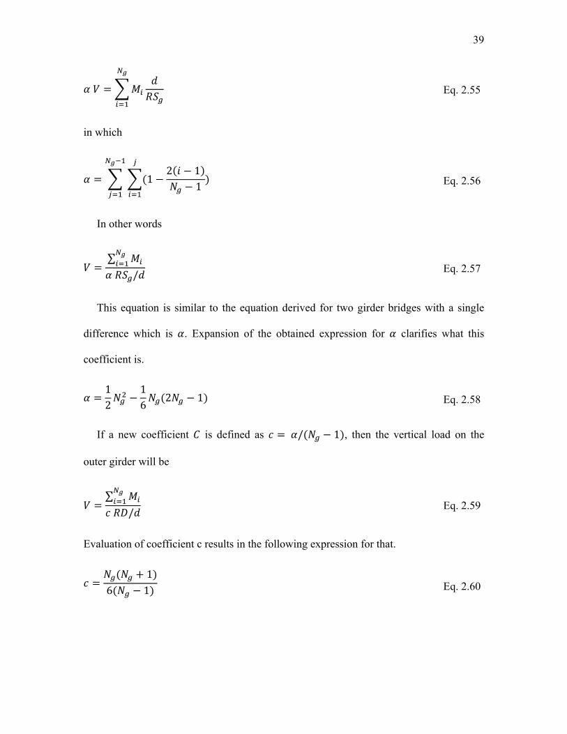
39
Eq. 2.55
in which
12 1
1 Eq. 2.56
In other words
∑ / Eq. 2.57
This equation is similar to the equation derived for two girder bridges with a single
difference which is . Expansion of the obtained expression for clarifies what this
coefficient is.
12
16 2 1 Eq. 2.58
If a new coefficient is defined as / 1 , then the vertical load on the
outer girder will be
∑ / Eq. 2.59
Evaluation of coefficient c results in the following expression for that.
16 1 Eq. 2.60

40
The value of the above equation for 2 is equal to unity which is in compliance
with the result of the study on two-girder bridges. The value of the coefficient for
different number of girders is tabulated in Table 2.5-1.
: Number of Girders C Factor
2 1.000
3 1.000
4 1.111
5 1.250
6 1.400
7 1.556
8 1.714
9 1.875
Table 2.5-1. C Factor for Different Number of Girders
As the first approximation, the summation of the girders moments can be estimated by
the sum of the moments due to applied loads. So, the Eq. 2.59 can be estimated by
∑ / Eq. 2.61
which directly gives the load applied to the outer girder at diaphragm location. The loads
on the other girders can be obtained by the linear variation assumption for the loads. In
this way, first based on the external loads that are applied to the bridge a set of additional
shear forces on the girders is calculated. Then, the girders are analyzed to obtain the
additional moments due to curvature.

41
2.6 Cross Frame Spacing
A criterion for cross frame spacing can be obtained from the equilibrium of horizontal
forces as stated in Eq. 2.41:
Eq. 2.62
in which is the horizontal force of cross frame with a spacing of due to bending
moment . Therefore, if the force of the cross frame is assumed to be distributed over
the spacing S, the magnitude of that force is:
Eq. 2.63
Since in a bridge, usually there are several cross frames along the length of the bridge,
if the force is assumed to be uniform between adjacent cross frames, the maximum
moment about the vertical axis in the flanges of the girder is:
12 12 Eq. 2.64
The moment tends to bend the flanges of the girder about the vertical axis. But the
direction of bending is different for top and bottom flanges, so that it causes some sort of
warping in the bridge girders. The longitudinal stress due to this lateral moment is equal
to the moments divided by the section modulus of the flange under consideration:
Eq. 2.65
where is the elastic section modulus of the flange equal to:

42
6 Eq. 2.66
On the other hand, the bending moment causes longitudinal stresses in the flanges
of the girder which can reasonably estimated as:
Eq. 2.67
Substitution of the above three equations into Eq. 2.64 results in:
2 Eq. 2.68
The ratio of the stresses due to lateral bending of the flange can be presumed by
designer in order to find an approximate spacing for the cross frames. Using the above
equation, the designer can find the optimum spacing of the cross frames after one or two
iterations.

43
Chapter 3
Detailed Study of Connections
in an Integral Abutment
3.1 Introduction
In this chapter, the behavior of the connections in the integral abutment of a steel
bridge is studied in details. For this purpose, first the general configuration of a typical
integral abutment is discussed. A picture of the details for this type of abutments which is
in practice in the US is presented. Then, the material models considered for steel and
concrete elements are investigated. Next, the finite element modeling of the abutment is
explained. And at the end, the results of the analysis are brought.
In order to study the integral abutments, finite element modeling is conducted using
the software package Abaqus 6.9.1. This general-purpose program is able to analyze such
structural details in the finest possible way. In the following sections, the method of
analysis is explained step by step.

44
3.2 Abutment Configuration
A general picture of an integral abutment of a steel I-girder bridge is depicted in
Figure 3.2-1. As can be seen, the concrete mass of the wall is continuous with the deck
slab. This is maybe the first reason that this type of abutment is called integral. In these
abutments, the steel girder is embedded in the concrete wall in a length of about half of
the wall thickness. It is supposed that the bond between steel and concrete which is
poured on it develops enough stresses for attaching the girder to the wall. Although the
horizontal rebars of the wall are continued through the web of the girder. There may also
be some shear studs attached to the bottom flange of the girder in the embedment length.
The purpose of installing such studs is to increase the reliability of the connection to
carry negative moments. The top flange of the girder is connected to the reinforced
concrete deck by shear connectors which altogether provide the tension component for
the presumed negative moment.
In these abutments, the piles are embedded in the concrete mass of the wall. The
connection is assumed to be provided by the bond of concrete and steel. The length of
embedment is typically between 2 and 4 feet. The wall rebars are so arranged that they do
not intersect with the piles.
The approach slab is attached to the abutment wall by means of a pin connection
detail. Therefore, it just applies a vertical load to the abutment wall and does not
participate in the overall response of the abutment. Because of that, it can be eliminated
from the study.

45
Figure 3.2-1. General Configuration of an Integral Abutment
3.3 Steel Material Modeling
The steel components of this connection include flanges and web of the girder,
stiffeners, steel pile and reinforcement of the concrete elements. ASTM Grade 50 steel is
assumed to be used in the girder and stiffeners. The H-piles are supposed to be of ASTM
Grade 36 steel and the rebars of concrete elements are of ASTM Grade 60 steel.
The strain-stress data of steel components are obtained from standard tension tests.
The results of such tests are the applied force and the strain of the specimen throughout
the time span of the test. So, having the initial cross sectional area of the specimen, the
resulted stress data would be based on that initial area. As for most practical engineering
purposes, the strains are so small that change of area is negligible; calculating the stress
based on initial area has adequate precision. The stress calculated using this method is
Pile
Concrete Wall
Approach Slab
Girder
Span
Deck
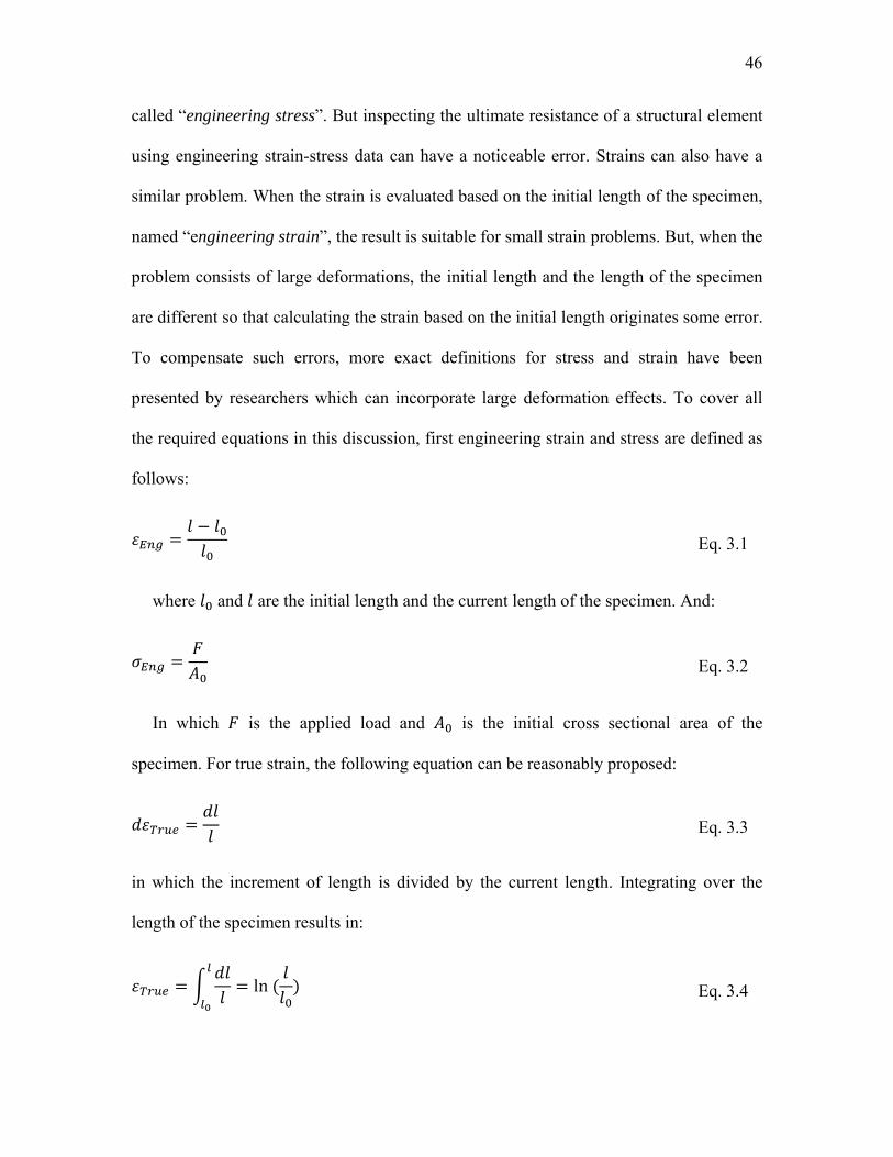
46
called “engineering stress”. But inspecting the ultimate resistance of a structural element
using engineering strain-stress data can have a noticeable error. Strains can also have a
similar problem. When the strain is evaluated based on the initial length of the specimen,
named “engineering strain”, the result is suitable for small strain problems. But, when the
problem consists of large deformations, the initial length and the length of the specimen
are different so that calculating the strain based on the initial length originates some error.
To compensate such errors, more exact definitions for stress and strain have been
presented by researchers which can incorporate large deformation effects. To cover all
the required equations in this discussion, first engineering strain and stress are defined as
follows:
Eq. 3.1
where and are the initial length and the current length of the specimen. And:
Eq. 3.2
In which is the applied load and is the initial cross sectional area of the
specimen. For true strain, the following equation can be reasonably proposed:
Eq. 3.3
in which the increment of length is divided by the current length. Integrating over the
length of the specimen results in:
ln Eq. 3.4

47
This strain is also called as log-strain. Substituting the engineering strain definition
into true strain definition yields a relationship between the two strains:
ln 1 ln 1 Eq. 3.5
Using the above equation, true strain can be easily calculated from the engineering
strain which is the result of the tension test. The true stress is also defined using a logical
equation:
Eq. 3.6
which is the division of the current force by the current area. The problem with the true
stress definition is that finding the real time area of the specimen during the tension test is
not possible using the conventional tension test equipments. Therefore, despite the
equation for calculating the true stress is available for engineers and designers, the
evaluation of true stress is not practical. So, researchers have tried to figure out methods
to estimate the true stress as precise as possible. The first recommended method to
evaluate the true stress is based on assuming constant volume for the element during
deformation. Using the previous equations for engineering and true strains and stresses
and also assuming a constant value for the element the following formulation can be
concluded for true stress:
1 Eq. 3.7
Using the above equation, the true stress can be easily calculated from engineering
strain and stress that are results of tension test. But, the validity of this equation depends

48
on the validity of the constant volume assumption. Another method to find the true stress
is based on the Poisson’s ratio approach. If a cylindrical specimen is under tension, the
area of the specimen is reduced while its length increases. If the ratio of the transverse
strain to longitudinal strain is assumed to be equal to the Poisson’s ratio, the current
diameter of the specimen will be:
∆ 1
1 Eq. 3.8
So, the current area will be:
4 1 1 Eq. 3.9
Therefore, the true stress can be written as follows:
1 1 Eq. 3.10
Using this equation the true stress is again evaluated as a function of engineering
strain and stress. This equation is valid if the ratio of the lateral to longitudinal strains is
equal to the assumed Poisson’s ratio. In this case, the validity of Poisson’s ratio after
yielding of steel and experiencing large strains is questionable.
3.3.1 Tension Test
To have a better understanding of the state of stresses in steel materials, the strain-
stress data of some actual tension tests that are conducted based the ASTM requirements
are studied. The tension tests have been done on test specimens with the dimensions in

49
accordance to ASTM A 370. The steel material for the specimens is ASTM A709, Grade
50 which conforms to the steel material of the girders of the studied bridges.
The first step of study is to plot engineering and true strain-stress curves for the
available tension test data. As there are two different definitions for the true stress, both
of the formulations are plotted. Figure 3.3-1 through Figure 3.3-4 show the strain-stress
curves.
Figure 3.3-1. Strain-Stress Curves (Tension Test # 1)
0
10
20
30
40
50
60
70
80
90
0 0.1 0.2 0.3 0.4 0.5
Stress (ksi)
Strain
Engineering
True (V=constant)
True (Poisson)
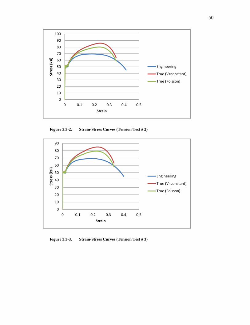
50
Figure 3.3-2. Strain-Stress Curves (Tension Test # 2)
Figure 3.3-3. Strain-Stress Curves (Tension Test # 3)
0
10
20
30
40
50
60
70
80
90
100
0 0.1 0.2 0.3 0.4 0.5
Stress (ksi)
Strain
Engineering
True (V=constant)
True (Poisson)
0
10
20
30
40
50
60
70
80
90
0 0.1 0.2 0.3 0.4 0.5
Stress (ksi)
Strain
Engineering
True (V=constant)
True (Poisson)

51
Figure 3.3-4. Strain-Stress Curves (Tension Test # 4)
As can be observed from the results of different tension tests, the equivalent true point
of each point of engineering curve has smaller strain value. This is attributed to the fact
that ln 1 is smaller than for nonzero values of strains. The other observation
is that engineering definition of stress gives the smallest stress and true definition with
constant volume assumption yields the largest stress among stress definitions. True stress
based on legitimacy of Poisson’s ratio results in stress values between the other two stress
definitions. An additional fact about strain-stress curves is that all of the different
approaches are approximately the same up to start of strain hardening of steel. This is a
very helpful remark in the practical designs where stresses are kept below the stress
plateau. The last but not the least observation from the above graphs is that the slope of
true strain-stress curve at the beginning of strain hardening region is about 1.18 times of
that slope in the engineering strain-stress curve. This ratio is the same for all conducted
tension tests.
0
10
20
30
40
50
60
70
80
90
0 0.1 0.2 0.3 0.4 0.5
Stress (ksi)
Strain
Engineering
True (V=constant)
True (Poisson)

52
3.3.2 Validity of Constant Volume Assumption
Further study on these curves is initiated by looking more exactly at the failure point
of the curves. As stated before, in normal tension tests, the applied force to the specimen
at each moment (usually with one second intervals) is recorded, while the actual strains in
the failure zone are not known. But, the cross sectional area of the specimen after break
can be measured. This cross section represents the actual cross section of the specimen at
the time of failure after elastic rebound of the area. Since the necked area shows a
tremendously large plastic deformation, the elastic rebound of the cross section can be
ignored in the calculations; however estimation of the elastic rebound is not a difficult
problem. For the previously discussed tension tests, the final cross sectional area of the
specimens are measured. These areas are 0.06396, 0.06558, .06710 and 0.06299 inch
squared for the tests #1 through #4, respectively. Dividing the ultimate forces by these
areas shows considerably different stress values at the very last moments of tension tests
compared to those of true strain-stress curves. These ultimate stresses are 134.3, 141.2,
137.3 and 139.9 ksi for the tests #1 to #4, respectively. As there is not any particular
assumption in calculating these stress values, it can be believed that these stresses are
more exact compared to true stresses which are calculated based on some assumptions.
At this point, since the true stress based on Poisson’s ratio assumption gives stress values
that are even less than those of the stress values based on constant volume assumption,
the Poisson’s ratio true stress is disregarded for the rest of the study and after this, the
true stress means the stress estimated based on constant volume assumption.
Another point of interest is the point of maximum stress on the engineering strain-
stress curve. As the engineering stress is obtained by simply dividing the applied force by

53
the initial cross sectional area, maximum stress at this point means maximum applied
load. Therefore, at this point the derivative of the applied load is zero:
0 Eq. 3.11
So
0 Eq. 3.12
And therefore
Eq. 3.13
On the other hand, constant volume assumption gives another expression for . As
the volume is constant, its derivative is zero. So
0 Eq. 3.14
Hence
Eq. 3.15
The second equation in the above expression is based on Eq. 3.3 which is the
definition of true strain. Thus
Eq. 3.16
Or
Eq. 3.17
In other words, the slope of the true strain-stress curve is equal to the value of true
stress at that point. This derivation is for the point of maximum stress on the engineering

54
strain-stress curve. This formulation is presented by Yakel (Yakel, 2009). To verify this
equation, the results of the available tension test are scrutinized. The results of tension
tests show that the slope of the strain-stress curve is on average 20 percent larger than the
value of true stress, at the point of maximum engineering stress.
1.2 Eq. 3.18
This is another reason that the constant volume assumption is not valid for large
deformations.
3.3.3 Elastic Rebound of Cross Section
In the previous section is was shown that the exact value of stress at the time of failure
in tension tests is much higher than those predicted by true stress formulation based on
the constant volume assumption. Those values of stress were calculated ignoring the
elastic rebound of the cross section after the specimen breaks. In this section, it is tried to
find the magnitude of the stresses considering the area of the specimens before the
rebound.
If the dimensions of a rectangular specimen after the break at failure section are
and , the area of the cross section is times . But
the cross sectional area right before the break is smaller than that. The elastic rebound of
the section can be estimated having the stress of the section at the time of the break. The
elastic rebound strain for each side of the specimen is equal to the stress at the moment of
break divided by the modulus of elasticity.

55
Eq. 3.19
So, the dimension of each side of the specimen just before failure is:
1 Eq. 3.20
And
1 Eq. 3.21
For circular specimens and are replaced by the measured diameter
. Consequently, a more exact cross sectional area for the specimen at the
moment of break can be obtained using the following equation:
1 Eq. 3.22
As is a function of and this stress is a function of the area
just before the break, an iterative procedure can be employed to find the area at the
moment of failure.
Examining the presented formulation for the available tension tests show that for
tension tests #1 through #4 the first iteration results in areas equal to 0.06337, 0.06494,
0.06647 and 0.06239 inch squared, respectively. The ratios of these areas to the measured
areas are 0.9907, 0.9903, 0.9905 and 0.9902. As the difference of the measured area and
the calculated area of the first iteration is less than one percent, other iterations are
ignored and the cross sectional area of the specimens at the time of break can be assumed
to be equal to %99 of the measured area after the break. This method is used for true
cross sectional area calculation for the rest of this study. Therefore the true stress at the

56
time of break is calculated by dividing the actual final load by %99 percent of the
measured area of the section after the break.
3.3.4 Proposing a New Model for Steel Material
Based on the previous discussions on the results of tension tests, a model for the true
strain-stress curve of steel material is presented in this section. The model assumes that
the engineering strain-stress data are available for the material under study. The purpose
is to define the true strain-stress curve. The model is described in the following steps. The
key points are designated in Figure 3.3-5:
Figure 3.3-5. Designation of the Key Points on the Strain-Stress Curves
Step 1- For the points on the elastic region and yielding plateau, it is assumed that the
constant volume assumption is valid and the values of true strain and true stress are
obtained by Eq. 3.5 and Eq. 3.7. Therefore points A, B and C are known.
A
B C
D
E
Stre
ss
Strain
Do
Engineering S-S
True S-S
E
max
1.2EST,Eng
D1.2

57
Step 2- The slope of true strain-stress curve at the beginning of strain hardening region
is assumed to be 1.18 (or approximately 1.2) times of that slope for engineering strain-
stress curve (as presented in Section 3.3.1).
Step 3- Point D is the corresponding true strain-true stress point for the point of
maximum stress on the engineering strain-stress curve based on constant volume
assumption (using Eq. 3.5 and Eq. 3.7).
Step 4- The slope of the true strain-stress curve at point D is equal to 1.2 times of the
value of true stress at that point (As discussed in section 3.3.2).
Step 5- A smooth curve is fitted between points C and D knowing the coordinates of
these points and the slope of the curve at these points. The curve fitting technique is
offered in the next section.
Step 6- A line is extended beyond point D with the same slope as the slope of the
curve at point D and terminated at point E with a stress level equal to the maximum true
stress at the moment of break. As discussed in Section 3.3.3, this stress is equal to the
applied load at the time of break divided by %99 of the cross sectional area after the
break.
3.3.5 Curve Fitting
In the material model proposed in the previous section, a curve was needed to fit
between points C and D. There are some requirements for the curve. The first one is the
smoothness of the curve. Rough changes are not seen in the engineering strain-stress
curve. So, a function having rough variations is not expected for the true strain-stress
curve in this region. The other necessity is that the function is concave between these two
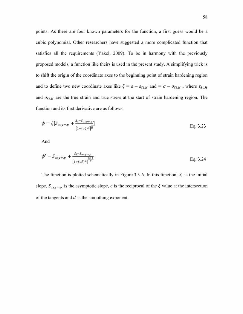
58
points. As there are four known parameters for the function, a first guess would be a
cubic polynomial. Other researchers have suggested a more complicated function that
satisfies all the requirements (Yakel, 2009). To be in harmony with the previously
proposed models, a function like theirs is used in the present study. A simplifying trick is
to shift the origin of the coordinate axes to the beginning point of strain hardening region
and to define two new coordinate axes like . and . , where .
and . are the true strain and true stress at the start of strain hardening region. The
function and its first derivative are as follows:
.. Eq. 3.23
And
.. Eq. 3.24
The function is plotted schematically in Figure 3.3-6. In this function, is the initial
slope, . is the asymptotic slope, is the reciprocal of the value at the intersection
of the tangents and is the smoothing exponent.

59
Figure 3.3-6. Scheme of Fitted Curve Between Points C and D
As there are four known values (the coordinates and the slopes at the two ends of the
curve) and four unknown values of , ., and , it seems that four equations can
be written to find the four unknown value. But, coordinates of the first end (0,0) is a
trivial solution for Eq. 3.23, independent of the four unknown values. Therefore, there is
one extra unknown value in this problem and assuming a value for one of them results in
a solution for the other three. Plotting different curves for different values of the involved
parameters shows that if the smoothing exponent is between 1 and 3, the curve fits the
best as what is expected for this transition function. If the exponent is less than 1, the
curve looks like a line and if it is larger than 3, the curve tends to the tangents of the two
ends. So, a value between 1 and 3 is chosen for that. Let’s take equal to 2.
Among the other unknown parameters, is the easiest to find. If 0 is plugged
into Eq. 3.24, then which shows is simply equal to the known slope of the first
end.
C
D end end
Si
Sasymp.
1/c

60
Now, there are two unknown parameters . and and two known values which
are the coordinates and slope of the end point. Plugging the coordinates of end point into
Eq. 3.23 and back-calculating yields:
.
.1 / Eq. 3.25
Simultaneous numerical solution of the Eq. 3.24 and Eq. 3.25, so that the slope at the
end is equal to the known value of slope, yields the values of . and . Figure 3.3-7
shows the curve for a smoothing exponent value of 2, an initial slope of 444 , a
final coordinates of , 0.1435 , 27.98 and an end slope of 98.2 . The
resulted values for . and are 88.71 and 22.24, respectively. Note that the end
slope and asymptotic slope are not the same.
Figure 3.3-7. Fitted Curve Between Points C and D
0
5
10
15
20
25
30
0 0.02 0.04 0.06 0.08 0.1 0.12 0.14 0.16
ψ(ksi)
ξ

61
3.3.6 A Sample Model: Grade 50 Steel
The result of all of the modeling steps for a Grade 50 steel is shown in Figure 3.3-8. In
this model, the curve is linear up to a stress of 50 ksi with a slope of 29000 ksi. The strain
at this point is 0.00172. After that, it has a plateau up to a strain of 0.0227. Note that the
slope of plateau is not a real zero. Then, on the transition curve, it goes to a strain of
0.1663 with a stress of 82.18 ksi. After the transition, it goes up linearly to a stress level
of about 141 ksi with a corresponding true strain of 0.767. Other steel materials are also
modeled using the same approach.
Figure 3.3-8. Material Model for Grade 50 Steel
3.4 Concrete Material Modeling
In this section, the behavior of concrete under loading is studied. Concrete shows a
very complex response when imposed to different loading conditions. There are several
factors that affect the response of concrete members. Concrete has totally different
0
20
40
60
80
100
120
140
160
0 0.1 0.2 0.3 0.4 0.5 0.6 0.7 0.8 0.9
s(ksi)
e
Total Strain
Plastic Strain

62
behaviors under compression and tension. Multi-axial load application is also a decisive
parameter. When concrete is confined by lateral compressive force, it can carry
considerably higher axial load. To study the material properties of concrete, first the
response of concrete under compressive forces is explained. Then the existing models to
predict the strain-stress properties of concrete specimens under compression are given.
Then, selecting one of the models, it is tried to illustrate how the model is perceived in
the finite element program, Abaqus. This program has some different methods to model
nonlinear strain-stress response of materials among which the most applicable one for
concrete behavior is detailed. The same steps are taken for tensile behavior of concrete.
For this purpose, first concrete response under tension is explained. Then, one of the
existing models for estimating the strain-stress curve of concrete under tension is
elucidated. And at the end, the technique of Abaqus to model the tensile behavior of
concrete is elaborated.
3.4.1 Concrete Response under Compression
When a concrete member is under compressive force, it demonstrates a nonlinear
strain-stress curve. In the first stages of loading, concrete stress goes up with an
approximately linear trend as the strain increases. But under greater loads, the rate of
stress increase reduces so that it reaches a maximum point. After that, the concrete stress
decreases as the displacement increases. At the final point, the concrete crushes due to
application of the ultimate compressive force. This behavior is not the same under
different conditions. When the rate of load application changes or multi-axial load is
applied to the concrete member, different strain-stress curves are resulted. The other fact

63
is that concretes of different strength show different crushing strains. Figure 3.4-1 shows
the strain-stress curves for some concrete specimens of different compressive strength.
Figure 3.4-1. Strain-Stress Curves of Concrete Specimens of Different Strength
It can be observed that the compressive stress is a nonlinear function of strain. Also,
the crushing strain decreases as the maximum stress increases. Finding the affecting
parameters and their nonlinear relation to the compressive strength is a complex task
which has been studied by several researchers. The next subsection discusses some their
works.
3.4.2 Concrete Compression Response Models
Several researchers have investigated the response of concrete in compression. The
result of their research has been to propose models for the strain-stress curve of concrete.
In this section, first these models are described and then a comparison of the models is
presented.

64
A) Hognestad Model
Hognestad (1951) proposed a model for the response of concrete under compression.
This model describes the stress of concrete at each strain level as a function of the
maximum compressive strength, , and the modulus of elasticity of concrete.
for 0 Eq. 3.26
Figure 3.4-2. Hognestad Model for Strain-Stress of Concrete in Compression
And
1 ..
for Eq. 3.27
In which
Eq. 3.28
Ec
f "c = 0.85f 'c
f "c = 0.15f "c
0 cu=0.004

65
B) Polynomial Model
This model describes the compressive stress of concrete as a polynomial function of
its strain. To find the constants of the polynomial functions, it is required to have some
assumptions. In the model, it is assumed that the maximum stress of the concrete takes
place at a strain equal to 0.002 and the failure occurs at the strain of 0.003. The other
assumption is on the failure stress level. In the current model it is assumed that failure
stress is 60 percent of the maximum stress. Implementing the above-mentioned
assumptions to a cubic polynomial, the following equation is resulted for the strain-stress
of the concrete.
5 10 5 10 800 Eq. 3.29
In which is the concrete stress and is the maximum compressive strength both in
ksi.
C) Carreira and Chu Model
Carreira and Chu (1985) proposed a curve for the strain-stress relation of concrete
which is compose of two parts. The first part is a line that is valid for stresses up to 30
percent of the maximum strength of the concrete. Beyond that point, a curve is suggested
that predicts the stress of concrete up to crushing strain. That curve is defined as follows.
Eq. 3.30
In which is the strain of concrete at the maximum stress of in MPA.
.1.55 Eq. 3.31

66
In this model, can be assumed to be equal to 0.002 and the crushing strain to be
equal to 0.003.
D) Comparison of Different Models
In this section, different models proposed for concrete compressive behavior are
compared to each other. For this purpose, the models are plotted for a concrete with
compressive strength of 4 ksi. The strain corresponding to this maximum stress is
assumed to be 0.002. The crushing strain is assumed to be 0.003. Figure 3.4-3 shows the
strain-stress curves predicted by different models.
As can be seen, up to the point of maximum stress, the Hognestad model and
Polynomial model are almost the same, while the model proposed by Carreira and Chu
predicts higher stresses. Beyond that point, Hognestad Model and Carreira and Chu
model have approximately the same stresses and the polynomial model drops the stresses
down to 60 percent of the maximum stress which was imposed to that model as an
assumption. Comparing this graph to Figure 3.4-1 shows that the stresses at the time of
failure are close to 80 percent of the maximum stress which is between the stress values
predicted by the polynomial model and the other two models. In the present study, the
model proposed by Carreira and Chu is used in the finite element models.

67
Figure 3.4-3. Strain-Stress Curves of Concrete in Compression in Different Models
3.4.3 Concrete Response under Tension
The behavior of concrete in tension is much more complicated than its behavior in
compression. When tensile strains are introduced in a concrete element, the stress starts
to be proportional to the magnitude of strain. For very small strains, the stress is
proportional to the strain, almost similar to the response under compression. But this
similarity is just for the early stages of loading. As the strain increases, complexities of
tensile behavior start to show up. The reason for that is formation of micro-cracks in the
body of the element in the tensile zone. The micro-cracks can unite to develop a macro-
crack which grows in the process of crack propagation. If the strain and average stress are
recorded during this process, it is observed that as the strain increases the average stress
over the tensile element decreases. The pattern for this reduction has been the subject of
study for several researchers who have recommended different models for the tension
stiffening regime of concrete behavior. More difficulty comes to existence when it is tried
00.51
1.52
2.53
3.54
4.5
0 0.001 0.002 0.003 0.004
s (ksi)
e
Concrete s‐e Curves in Compression
Polynomial
Carreira‐Chu
Hognestad

68
to express stress tensor in terms of strain tensor of at a point. Results of the studies show
that for such a material the stress tensor is not just a function of the strain tensor of that
point. But also, a strain field should be considered for the neighborhood of each point of
the element. The next subsection presents some of the existing models for the tensile
response of concrete.
3.4.4 Concrete Tension Response Models
Several researchers have studied the behavior of concrete in tension. Figure 3.4-4
shows the strain-stress curves which are proposed by some of the researchers. As can be
seen, linear, bi-linear and nonlinear descriptions are the recommendation of different
researchers for the tension stiffening part of concrete strain-stress curve. Bazant has
proposed a line for the tension stiffening part of the curve. Gylltoft has suggested the
stress as a bilinear function of the strain while some others like Scanlon, Mazars and Lin
& Scordelis have recommended curvilinear functions for that region of the response.
Figure 3.4-4. Strain-Stress Curves of Concrete in Tension in Different Models
max
u
Lin-Scordelis and Mazars
Bazant and Oh
Gylltoft
Scanlon

69
In this section, one of the existing models for predicting the post-cracking response of
concrete in tension is studied in more details. This method is recommended by Barros et
al. and is developed to consider both linear and exponential functions for the tension
stiffening of behavior of concrete (Barros, Martins, & Ferreira, 2001). That’s why the
formulations are given for both functions simultaneously. The assumed linear and
exponential functions for strain-stress curve are as follows:
Linear Function Eq. 3.32
And
Exponential Function Eq. 3.33
In which is the initial cracking stress, E is modulus of elasticity of undamaged
concrete, is the ultimate strain in tension and b is the calibration coefficient for the
exponential curve. If the above stress functions are plotted against strain, the schematic
shapes of Figure 3.4-5 are obtained. The unknown values and are found as follows.
Figure 3.4-5. Schematic Strain-Stress Curve of Concrete in Tension
ft
tu
Linear Model
Exponential Model
70
The area under the curves for these two functions will be equal to:
for Linear Function Eq. 3.34
And
for Exponential Function Eq. 3.35
On the other hand, the total area of the strain-stress curve is equal to the deformation
energy per unit volume, . From the definitions of Fracture Mechanics, one can obtain
the crack propagation energy per unit area of the crack as:
. Eq. 3.36
in which w is the width of the damaged region. As is a material property which can
be found for the customary materials in the fracture mechanics references, the area under
the strain-stress curve can be set equal to the known value of / .
Ozblot and Bazant recommend that the width of the damaged region is proportional to
the maximum aggregate size, which is a known parameter for any kind of concrete used
in the construction industry (Ozbolt & Bazant, 1996). So, can be assumed as a known
parameter as:
. Eq. 3.37
where is a factor changing between 3 and 8 and is the maximum aggregate
size.

71
As and are known, the area under the strain-stress curve can be set equal to the
ratio of / to find the unknowns of each of the two linear or exponential approaches.
For the linear function the unknown will be found as follows:
/ Eq. 3.38
So
Eq. 3.39
And for the exponential function the parameter will be calculated as follows:
Eq. 3.40
Therefore
Eq. 3.41
Hence, the tension stiffening part of the strain-stress curve for concrete will be:
Linear Function Eq. 3.42
And
Exponential Function Eq. 3.43
In practical cases, the strain cannot go to infinity, while in the exponential function
there is no limit for the strain. Therefore, to find an upper bound for the strain in the
exponential model, the area under the curve at the maximum practical strain is set equal
to 98 percent of the total area under the curve. This equality results in a strain of as

72
the maximum practical strain. So for the exponential function the range of applicability is
as follows:
Eq. 3.44
3.4.5 Concrete Response Modeling in Abaqus
To study the integral abutment connections, the finite element program Abaqus is
used. The program has several capabilities, making the user able to model complex
structural systems. Regarding the concrete nonlinear structural properties, two major
methods are available in the program. One of them is smeared crack modeling and the
other one is concrete damaged plasticity. In the present study, concrete damaged
plasticity is employed as the method of analyzing the problem. The accuracy of this
approach to model the behavior of reinforced concrete has been verified by many
researchers in the past years.
Concrete damaged plasticity can incorporate two types of concrete failure in the
model: crushing under compressive stresses and cracking under tensile stresses. Crushing
and cracking are detected when certain criteria reach yield surfaces. The yield surfaces
are defined by compressive and tensile equivalent plastic strains as the hardening
parameters. In the coming discussion, these two parameters are shown by and .
Figure 3.4-6 illustrates the strain-stress curves of concrete in tension and compression. It
is observed that as the strain increases, the tensile stress increases linearly up to a
maximum tensile stress of . Beyond this point, the tension softening starts which
results in reduction of stress for any increment of strain so that in very large strains the

73
stress of concrete tends to zero. In compression the response is different. In the
beginning, the stress has a linear relationship with strain up to reaching the stress of .
After that, stress goes up as the strain increases in a nonlinear manner. This trend is seen
up to a maximum compressive capacity of . Beyond this maximum point, the strain
softening part of the curve starts which results in lower stresses for larger strains. This
response continues so that for very large strains, the compressive stress of concrete goes
to zero.
Figure 3.4-6. Strain-Stress Curves of Concrete in Tension and Compression
t0
t
t
tel
tpl
Eo
Tension
(1-d )t Eo
cu
c
c0
cel
cpl c
Eo(1-d )c Eo
Compression

74
Concrete damaged plasticity is supposed to model damage in concrete in compression
and tension. This is considered in this approach by decreasing the stiffness of concrete
when strain softening starts in compression or tension. This is implemented in the model
by means of damage parameters in compression and tension designated by and ,
respectively. These parameters reduce the modulus of elasticity of concrete and can be
between zero and one. Values of damage parameter close to zero represent early stages of
softening and values closed to one correspond to very low stiffness which is seen at large
strains. Values of these parameters very close to one can lead to structural and so
numerical instabilities in the problem.
The problem of concrete damage is more complex when dealing with cyclic loads. In
this case, some cracks are initiated when the material is under tension. Then, compression
in the next cycles of loading may result in closure of some of the cracks. Therefore, some
part of the lost stiffness of the concrete may be reinstated. This complicated behavior is
modeled by recovery parameters in compression or tension.
Another difficult situation occurs when concrete is under multi-axial state of stress. In
this case, Abaqus makes use failure surfaces instead of failure curves. Figure 3.4-7
shows a section of the failure surface for the case of biaxial loading. In this picture the
points of failure corresponding to uniaxial compression, uniaxial tension, biaxial
compression and biaxial tension are demonstrated.

75
Figure 3.4-7. Biaxial Failure Surface of Concrete
In concrete damaged plasticity model, the behavior of concrete under compression is
idealized by defining the inelastic strain of concrete. This strain is equal to the total strain
minus the elastic strain assuming an undamaged modulus of elasticity for concrete.
Eq. 3.45
In which
Eq. 3.46

76
Figure 3.4-8 shows the definition of compressive inelastic strain based on the above
equation. Also elastic and plastic strains are illustrated in the picture, to clearly show the
difference of inelastic strain and plastic strain.
Figure 3.4-8. Definition of Compressive Inelastic strain Used for Definition of
Compression Hardening Data (Abaqus Documentation)
The same approach is used for tension stiffening part of the strain-stress response of
concrete. The input data of Abaqus are post-cracking stress and also cracking strain for
an element in tension. The cracking strain is defined as the total tensile strain minus the
elastic strain assuming undamaged modulus of elasticity for concrete. Therefore:
Eq. 3.47
In which
Eq. 3.48
cu
c
co
cel
cpl
cin
ocel c
Eo
Eo
(1-d )c Eo

77
Figure 3.4-9 illustrats the cracking strain based on using undamaged modulus of
elasticity to obtain it from total strain. To distinguish the difference of cracking strain and
plastic strain, both of them are shown in the picture. As can be seen, plastic strain is
calculated using the reduced modulus of elasticity of the damaged material. An initial
guess for the tension stiffening part of the curve which is recommended in Abaqus
Documentation is a line originating from a strain of 10E-4 for a stress of and ending
to a point of zero stress for a strain of 10E-3. Other more accurate models for tension
stiffening can be found in the literature.
Figure 3.4-9. Definition of Tensile Cracking Strain used for Definition of Tension
Stiffening Data
3.4.6 Employed Concrete Models
Based on the previous discussions on the behavior of concrete elements in
compression and tension, the following models are developed for a 4ksi concrete which is
used in the finite element analyses. Figure 3.4-10 shows the total strain and also the
t0
t
t
tel
tpl
Eo
(1-d )t Eo
tck
otel
Eo

78
inelastic strain of concrete in compression versus stress, which is based on Carreira and
Chu model. As can be observed, there are no inelastic behavior up to the stress of 1.2 ksi.
Figure 3.4-10. Total and Inelastic Strain vs. Stress for 4 ksi Concrete in Compression
Figure 3.4-11 depicts the total and cracking strain of the concrete material versus its
tensile stress. The employed model in tension is an exponential one. It shows that the
concrete material does not have an inelastic response up to reaching a tensile stress level
of about 0.5 ksi. Then, it starts to develop cracks which results in steep drop of its tensile
strength.
0.0
0.5
1.0
1.5
2.0
2.5
3.0
3.5
4.0
4.5
0 0.0005 0.001 0.0015 0.002 0.0025 0.003 0.0035
Stress(ksi)
e
Total Strain
Inelastic Strain

79
Figure 3.4-11. Total and Cracking Strain vs. Stress for 4 ksi Concrete in Tension
3.5 Elements
In this section, a brief explanation on the elements that are used in the finite element
modeling is presented. The descriptions are based on Abaqus 6.9 HTML Documentation.
For more details one can refer to the Abaqus Documentation.
3.5.1 C3D8(R)
C3D8 is an 8-node linear brick element. C3D8R is an 8-node linear brick element with
reduced integration and hourglass control. These elements have three degrees of freedom
at each node which are translations in x, y and z directions. Figure 3.5-1 shows a picture
of these elements. The extension R stands for reduced integration. Reduced integration
means an integration scheme which is one order less than the full integration scheme
which is used for integration of internal forces and stiffness of the element. Reduced
integration reduces the constraints introduced by an element when the continuum theory
being modeled has some sort of internal constraints, like incompressibility or the
0.000
0.100
0.200
0.300
0.400
0.500
0.600
0 0.001 0.002 0.003 0.004 0.005 0.006
Stress (ksi)
Strain
Cracking Strain
Total Strain

80
Kirchhoff transverse shear constraints when solid elements are used in order to analyze a
bending problem. In these applications, full integration leads to locking which means
resulting in a response that is orders of magnitude too stiff, so that the results are totally
unusable. In such cases, reduced integration will often work well. In contrast, if there is
no R in the element name, it is fully integrated. It means the Gauss scheme chosen will
integrate the stiffness matrix of the elements with uniform material behavior exactly if
the Jacobian of the mapping from the isoparametric coordinates to the physical
coordinates is constant throughout the element. The meaning of this statement is that the
opposite sides or faces in 3D elements must be parallel and in second-order elements the
nodes must be either at the ends or middle of the element sides. Hourglassing can be a
problem with first-order, reduced-integration elements, like C3D8R, in stress-
displacement analyses. Since the elements have only one integration point, distortion is
possible in such a way that the strains calculated at the integration point are all equal to
zero, that leads to uncontrolled mesh distortion. First-order, reduced-integration elements
in Abaqus include hourglass control, but reasonably fine meshes should be used for them.
By distributing point loads and boundary conditions over a number of neighboring nodes,
instead of one point, the hourglassing can be minimized.
Figure 3.5-1. C3D8 Brick Element
8-node linear element

81
3.5.2 C3D4
C3D4 is a 4-node first-order constant stress tetrahedral element. It is tried to avoid
using this element, but is some cases making use of it has been inevitable.
3.5.3 C3D10M
C3D10M is a 10-node modified tetrahedron element with hourglass control.
Figure 3.5-2 illustrates this element.
Figure 3.5-2. C3D10M Tetrahedron Element
3.5.4 T3D2
T3D2 is a 2-node linear displacement element. The behavior of this element is the
same as truss elements is structures. It carries only axial load. No shear or bending
moment is transferred by this element. This element, when embedded in a concrete mass,
can be regarded as a rebar.
3.6 Stress Functions Definition
In this section, the definitions of the stress functions that are used in the following
discussions are presented. The stress components at each node are assumed to be given
10-node modified second-order element

82
by the Cauchy stress tensor which its elements are . The isotropic invariants of the
stress tensor are defined as
Eq. 3.49
Another set of invariants are defined as
Eq. 3.50
If the principal stresses of T are , and , the above six invariants can be written
in terms of these stresses as
Eq. 3.51
And
Eq. 3.52

83
The deviatoric stress which has a crucial role in plasticity theory is defined as the
difference of Cauchy stress and the spherical stress as
T Eq. 3.53
In which the average stress is
T Eq. 3.54
A useful property of the deviatoric stress is that its trace is equal to zero.
T T 3 0 Eq. 3.55
The isotropic invariants can also be defined for the deviatoric stress in the same way
as defined for the Cauchy stress:
Eq. 3.56
And the second set of invariants as follows:
0
Eq. 3.57
The latter set of invariants of deviatoric stress are written in terms of the invariants of
Cauchy stress as
0 Eq. 3.58

84
3
2 9 27
One of the most celebrated yield criteria for ductile metals is the Von Mises Yield
function as follows
Eq. 3.59
In which is the yield stress of the ductile metal material and is Von Mises
stress potential defined as
: Eq. 3.60
Plugging from Eq. 3.57 into Eq. 3.60 yields
3 Eq. 3.61
Substituting from Eq. 3.58 into Eq. 3.61and making use of Eq. 3.52 to convert
invariants of Cauchy stress into principal stresses gives Von Mises stress potential as a
function of principal stresses as
Eq. 3.62
One of the most significant advantages of the above equation is that it proves that
Mises stress potential can be smaller or larger than the principal stresses and when one of
the principal stresses is much larger than the other two, Mises stress is close to the
absolute value of that larger stress.
As the Mises stress potential is always equal to or greater than zero, another equivalent
stress definition by means of which the direction of traction vector can be distinguished is

85
also required. This criterion can be achieved using the third invariant of the deviatoric
stress tensors. This third invariant is defined as
. : Eq. 3.63
This value is a useful representation of the stress values at a specific location which its
sign can be positive or negative. In the following study, this third invariant of deviatoric
stress will be used to distinguish tensile or compressive stresses when required.
3.7 Finite Element Modeling
An elaborated technique is employed to model the abutment details in Abaqus 6.9.1.
The abutment wall, deck slab, haunch, girder, stiffeners and piles are modeled using 3D
solid elements. Rebars are modeled by means of 2-node 3D truss elements. Figure 3.7-1
shows a general picture of the abutment which consists of different elements.

86
Figure 3.7-1. General Configuration of the Integral Abutment Model
Figure 3.7-2 shows the girder element of the connection. The girder is made of Grade
50 steel. It has an 18”x1.5” top flange, a 66”x0.5” web and an 18”x2” bottom flange. The
girder may have two stiffener plates at the face of the concrete wall. The stiffener size is
66”x8.75”x0.5” on each side.

87
Figure 3.7-2. Girder Element of the Connection
The girder is 18 inches embedded in the abutment wall. Figure 3.7-3 illustrates the end
of the girder which is embedded in the wall and cannot be seen clearly in the other
pictures. One of the features of such connections is that the rebars of the abutment wall
go through the web of the girder. This requires the web of the girder be drilled to provide
the holes for rebars to go through. As the two top rebars are #7 and the lower five rebars
are #5, the upper two holes are larger than the lower ones.

88
Figure 3.7-3. Embedded End of the Girder
Figure 3.7-4 shows the highlighted picture of the girder in the connection. The
boundaries of the girder element can be visibly seen in this picture.

89
Figure 3.7-4. Highlighted Position of the Girder Element
Figure 3.7-5 shows the abutment wall part of the connection. It is made of concrete
material with a characteristic strength of 4 ksi. It has a width of 42”, a length of 108” and
a height of 136”. The place of girder and piles embedment is cut into the wall using the
outstanding features of Abaqus. As the girder stiffeners are assumed to be inside the mass
of concrete, their place is also cut in the wall element.

90
Figure 3.7-5. Concrete Wall of the Abutment
Figure 3.7-6 illustrates the highlighted picture of the abutment wall which more
clearly shows its boundaries and also the place of piles embedment in the wall.

91
Figure 3.7-6. Highlighted Position of the Abutment Wall
Figure 3.7-7 shows the highlighted position of the deck in the abutment assembly.
Like the abutment wall, it is made of class BD47 4 ksi concrete. The deck has an 8”
thickness and has a tributary width of 108” for each girder.
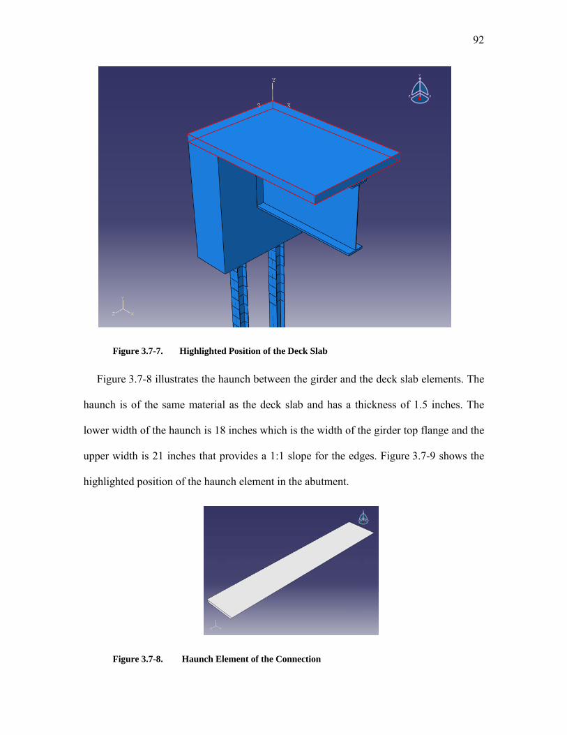
92
Figure 3.7-7. Highlighted Position of the Deck Slab
Figure 3.7-8 illustrates the haunch between the girder and the deck slab elements. The
haunch is of the same material as the deck slab and has a thickness of 1.5 inches. The
lower width of the haunch is 18 inches which is the width of the girder top flange and the
upper width is 21 inches that provides a 1:1 slope for the edges. Figure 3.7-9 shows the
highlighted position of the haunch element in the abutment.
Figure 3.7-8. Haunch Element of the Connection

93
Figure 3.7-9. Highlighted Position of the Haunch
Figure 3.7-10 shows the pile element of the abutment. The section of the piles is
H12x53 which is made of Grade 36 steel. The piles are modeled 3 feet below the point of
fixity. The abutment is supported by two piles which are 54 inches apart. The center of
the piles is 12 inches away from the front face of the wall. The surrounding soil of the
piles is modeled using the spring element in Abaqus. The stiffness of the springs is 4 k/in
per linear foot of the piles.

94
Figure 3.7-10. H- Pile Element of the Connection
Figure 3.7-11 shows the highlighted picture of the piles in the abutment assembly. The
embedded length of the pile in the abutment wall can be obviously detected in this
picture.

95
Figure 3.7-11. Highlighted Position of the H-Piles
Figure 3.7-12 shows the highlighted rebars of the concrete deck slab. The longitudinal
bars are #5 placed at 8” spacing at top and bottom layers. The transverse bars are #5 at
12” spacing again at both top and bottom layers. The cover above the upper transverse
rebars is 2 inches and the cover below the lower transverse rebars is 1 inch.

96
Figure 3.7-12. Highlighted Rebars of the Deck Slab
Figure 3.7-13 illustrates the abutment wall cage of reinforcement. The top and bottom
layer of bars along the length of the abutment consist of 4#7 rebar. The size of all other
rebars of the wall is #5. The rebars are not evenly distributed to minimize the intersection
with the girder or the piles. Although, some of them that are parallel to the wall face go
through the girder web as explained before. The clear concrete cover for the lower and
back face of the wall is 3 inches, while it is 2 inches for the front face of the wall. The
vertical rebars of the wall enter the deck slab to guaranty the load transfer between the
deck and the wall. However, a considerable portion of the load is supposed to be
transferred through the girder which is attached both to the deck and the wall.

97
Figure 3.7-13. Highlighted Rebars of the Abutment Wall
The effect of shear studs on the bottom flange of the girder in the embedded length is
also studied. Figure 3.7-14 shows two pictures of the shear studs below the bottom
flange.
Figure 3.7-14. Shear Studs Attached to the Girder Bottom Flange

98
Using the above-mentioned elements two different models have been made. The first
one is a single span bridge of 100 feet length which has integral abutments at the two
ends. The piles in this model are not modeled and a fixed support is provided for the
abutment wall. Using this model one is able to apply the ultimate gravity load to the
bridge and observe the behavior of the I-girder to abutment wall connection. The other
model is a 30 feet cantilever composite I-girder that is integrally connected to the
abutment. In the latter study, the piles are included in the modeling. So, it is possible to
investigate the pile-to-wall connection which is another area of interest. The following
sections of this chapter describe the results of analyzing these two models.
3.8 Moment Capacity of the Superstructure
Before proceeding to the results of finite element analysis, to have a measure of the
capacity of the superstructure section that is attached to the abutment wall, a moment-
curvature analysis of the section is performed using the defined material properties. A
MATLAB code is provided to analyze the section. The implemented approach in the
program is to increase the bending strain in the section incrementally and calculate the
imposed curvature and the developed moment in the section. This MATLAB program
has been a huge project by its own, and for brevity more explanation is avoided and the
program is brought in Appendix B.
Figure 3.8-1 shows the superstructure section for which the moment capacity is
calculated and Figure 3.8-2 illustrates the moment-curvature diagram of that section. It is
seen that the yielding moment of the section is about 160,000 k.in and the ultimate
moment capacity of the section is approximately 175,000 k.in.

99
Figure 3.8-1. Superstructure Section at the Vicinity of Abutment Wall (Section A-A)
Figure 3.8-2. Moment–Curvature of the Superstructure at Section A-A
Span
A
A
GirderSteel
Reinforce Concrete Deck

100
Figure 3.8-3 shows the stress distribution in the superstructure section when the
maximum moment is reached. It is observed that the neutral axis is 42 inches above the
bottom fiber of the girder. Other than about 3.5 inches below and above this neutral axis,
all other parts of the girder are yielding which have stresses equal or greater than 50 ksi.
Concrete deck is fully cracked and the upper and lower layers of rebars in the deck are
yielding. The stress of the rebars is more than 60 ksi. Note that the slope of the plateau
region in the presented steel material models in section 3.3 is not zero. That’s why the
stresses after yielding get larger than 50 and 60 ksi for Grade 50 and Grade 60 steel,
respectively.
Figure 3.8-3. Stress Distribution in the Superstructure at the Vicinity of Abutment Wall
Corresponding to Maximum Moment Capacity
0
10
20
30
40
50
60
70
80
‐60 ‐40 ‐20 0 20 40 60 80
Elevation (in
)
Stress (ksi)

101
3.9 Results of Analysis
The results of nonlinear finite element analysis of the studied integral abutment detail
are presented in this section. First, the steel I-girder stresses are discussed. This includes
the girder stresses at the vicinity of the abutment wall face, both in the embedded region
and outside of the wall. Then, the concrete deck stresses are shown. In the next step, a
discussion on the stresses of the abutment wall is presented. As a result, the effect of
girder stiffener right at the wall front face section is investigated. After that comes
another outcome of this study which is to show the effect of shear studs attached to the
bottom flange of the girder. One more investigation is on the pile stresses. Stresses of
abutment wall at the neighborhood of the pile are then illustrated followed by an
argument on necessity of a pile stiffener at that location.
3.9.1 Girder Stresses
In this section, the stress state of a girder integrally attached to an abutment wall is
studied. First, a 100-foot span bridge is analyzed in which the girder has no stiffener and
no bottom flange shear connectors. The Mises stresses for such a girder are depicted in
Figure 3.9-1. It is seen that the maximum stress happen in the web above the wall face.
At the level of loading corresponding to this picture, the concrete in contact to the end of
the bottom flange started crushing while the stress in the girder flange is much lower than
its yield capacity. To find a solution to decrease the web stresses and shift them to the
bottom flange, two usual details are described in the following sections.

102
Figure 3.9-1. Mises Stresses of Girder without any Stiffener or End Shear Stud
A) Effect of Girder Stiffener
In this part of the study, a transverse stiffener is added to the girder right above the
wall front face and the single span bridge is analyzed. Figure 3.9-2 describes the stresses
after adding the stiffener. It is observed that the stiffener reduces the web stresses to some
extents. But, as expected, the stiffener is not able to move the maximum stresses to the
bottom flange. That’s why some designers think about connecting shear studs to the
bottom flange to increase the moment carrying capacity of the girder. This problem is
discussed in the next section. The effect of the stiffener on the abutment wall stresses is
studied in section 3.9.2.

103
Figure 3.9-2. Mises Stresses of Girder with Stiffener without End Shear Stud
B) Effect of Girder End Shear Studs
Another idea is to connect shear studs to the bottom flange of the girder in the
embedded length to offer it a more pronounced role in carrying loads. Nine shear studs of
6 inches length and 1 inch diameter are tied to the lower face of the bottom flange.
Figure 3.9-3 shows the Mises stresses of the girder end. Comparing to Figure 3.9-1, it can
be observed that there is not a noticeable difference between the state of stress of the
girder with and without shear connectors. The maximum stress occurs in the web while

104
the shear studs are not able to give the bottom flange an added value. The effect of the
shear studs on the state of stress in the abutment wall is discussed in section 3.9.2.
Figure 3.9-3. Mises Stresses of Girder with End Shear Stud without Stiffener
C) Ultimate Loading
Another job is to analyze the single span bridge under heavy gravity loads and observe
the behavior of the connection. The loading and analysis are continued up to reaching
plastic moment capacity in the middle of the 100-foot span. As can be observed in
Figure 3.9-4, the Mises stresses in the girder are about 50 ksi from the bottom fiber of the
section up to upper portion of the web. Figure 3.9-5 is showing the Mises stresses of the
concrete deck. The concrete stress at mid-span is close to 4 ksi which is the maximum

105
strength of concrete. This configuration for stresses at mid-span corresponds to the plastic
capacity with the neutral axis below the top flange of the girder.
Figure 3.9-4. Mises Stresses of Half of the Girder

106
Figure 3.9-5. Mises Stresses of Concrete Deck
A closer look at the stresses of girder ends demonstrates that the girder has low
stresses at the ends, despite of plastification at mid-span. And another weird observation
is that the maximum stresses of the girder at the ends do not form in the top or bottom
flange. In integral abutment connections, the maximum stress at the girder end is in the
web above the wall front face. Figure 3.9-1 through Figure 3.9-3 show initiation of high
stresses in the web instead of flanges in such a connection. This is attributed to the
occurrence of knife edge phenomenon. In such connections, the girder web tends to cut
the face of the concrete wall like a knife. The other characteristic of these connections is
that the responsibility of developing the longitudinal stresses in the bottom flange of the
girder is with the surrounding concrete of the flange in the short practical lengths of

107
embedment. As the maximum supporting stress at the end face of the flange is the
capacity of concrete and the mobilized stress over the surfaces of the flange in the
embedded region is the friction and bond between steel and concrete, these two cannot
create stresses comparable to yield stress of steel material. Figure 3.9-6 shows the Mises
stresses of the girder end as the load is increased. It is observed that application of a large
load creates high shear stresses in the web of the girder while the stress in the bottom
flange of the girder is still low.
Figure 3.9-6. Mises Stresses of Girder’s End Corresponding to Mid-span Plastification

108
3.9.2 Abutment Wall Stresses At Girder Embedment
Zone
In this section, the concrete abutment wall stresses are studied in more details. The
first point of interest in the wall is the contact region of the steel girder and the wall. This
region is in charge of transferring the girder end shear and moment to the abutment
structure. As shown in Figure 3.9-7, maximum stresses are developed right below the
girder web at the face of the concrete wall. This picture is of wall supporting an
unstiffened girder. This region is subject to the vertical shear force and the horizontal
friction and bond between steel and concrete. This part of the abutment structure is
potential to failure because of this high stress and the limited confinement of concrete.
Figure 3.9-7. Mises Stresses of Abutment Wall Supporting an Unstiffened Girder
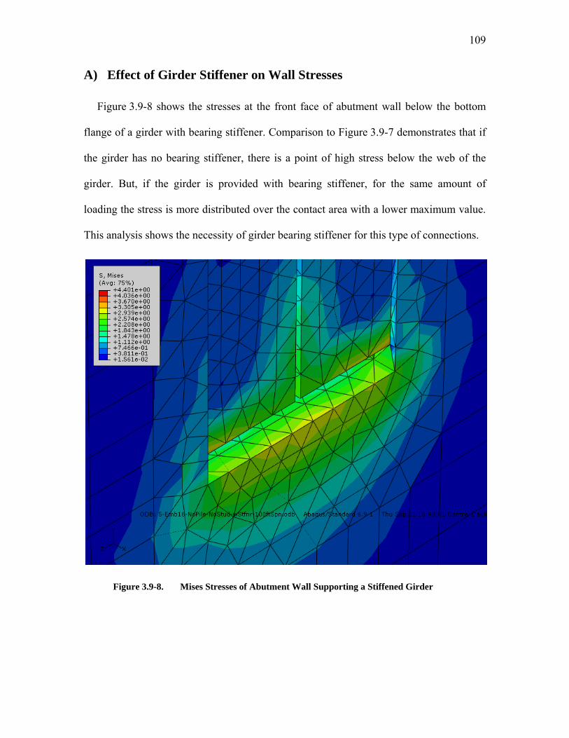
109
A) Effect of Girder Stiffener on Wall Stresses
Figure 3.9-8 shows the stresses at the front face of abutment wall below the bottom
flange of a girder with bearing stiffener. Comparison to Figure 3.9-7 demonstrates that if
the girder has no bearing stiffener, there is a point of high stress below the web of the
girder. But, if the girder is provided with bearing stiffener, for the same amount of
loading the stress is more distributed over the contact area with a lower maximum value.
This analysis shows the necessity of girder bearing stiffener for this type of connections.
Figure 3.9-8. Mises Stresses of Abutment Wall Supporting a Stiffened Girder

110
B) Effect of Girder End Shear Studs
Another study is to investigate the effectiveness and necessity of girder end shear
studs. In this study, the role of bottom flange shear connectors in changing the wall
stresses is examines. The Mises stresses of the girder and abutment wall in two different
cases of with and without shear studs are shown in Figure 3.9-9 and Figure 3.9-10. It
demonstrates that if shear studs are added to the bottom flange of the girder, the concrete
stresses at the end of the bottom flange decreases from 6.69 ksi to 4.61 ksi. In section
3.9.1, it was shown that girder stresses are not affected considerably by the end shear
studs. But, the results for abutment wall stresses show that the shear studs are effective in
mitigating the wall stresses.
A closer look at the wall stresses in this zone reveals that the maximum stress occurs
where the end of the bottom flange pushes the adjacent concrete. As the friction and bond
between the surfaces of the bottom flange do not mobilize high values of stress in the
bottom flange, development of stress in the bottom flange is mainly done by the concrete
in contact to the end face of the flange. While adding shear studs to the bottom flange,
helps engage a larger chunk of concrete in developing flange stresses.

111
Figure 3.9-9. Mises Stresses of Abutment Wall - Girder without End Shear Studs
Figure 3.9-10. Mises Stresses of Abutment Wall - Girder with End Shear Studs

112
3.9.3 Abutment Wall Stresses At Pile Embedment Zone
In the case of girder to wall connection, it was observed that the stresses in the
concrete wall at the points of contact to steel girder were so large. Therefore, it is also
expected that the stresses in the concrete in contact with steel piles to be high. Figure 3.9-
11 shows the stresses of concrete around the piles. As anticipated, large compressive
stresses are created at the lower face of the wall. Although there is a great gradient of the
stresses in depth, these stresses are so huge that are able to crush the concrete. Hence, a
detail to prevent the crushing is required. A suggestion can be to add stiffeners to the pile
at the concrete face section which will be discussed in the following section.
Figure 3.9-11. Mises Stresses of the Concrete Wall Around the Piles

113
A) Effect of Pile Stiffener
The finite element model of the abutment is run again by adding a pair of stiffeners to
the HP sections of the pile at the concrete lower face section. Figure 3.9-12 shows a
picture of pile stiffener. The stiffener has 0.5 inch thickness.
Figure 3.9-12. Stiffened Pile at the Wall Lower Face Section
As can be observed from Figure 3.9-13, the maximum stress of the concrete wall
reduces to 5.31 ksi. It shows about 18 percent of reduction of the stresses. These
stiffeners do not have a magnificent role in distributing the stresses in the concrete. As
opposed to the case of girder-to-wall connection, this time adding stiffeners is not so
effective.

114
Figure 3.9-13. Mises Stresses of the Concrete Wall Around the Piles with Stiffener
3.9.4 Pile Stresses
In the conventional detail for integral abutments, the weakest elements are the piles.
These piles are usually HP sections. The strongest HP section is HP14x117 which
compared to the other attached elements which are the girders and abutment wall is tiny.
That’s why these abutments absorb a small negative moment in comparison with the
capacity of the girders. Figure 3.9-14 shows the Mises stresses of the piles. The stresses
illustrate a full plastic hinge in the piles just below the lower face of the concrete wall.
The pile stresses start to reduce inside the wall as the distance to the concrete face gets
larger. The stress at the top section of the pile is close to zero.

115
Figure 3.9-14. Mises Stresses of Abutment Piles
A) Effect of Pile Stiffener
The stresses of the piles after adding the stiffeners are illustrated in Figure 3.9-15.
Comparing to Figure 3.9-14 reveals that there is a slight difference between the pile
stresses with and without stiffeners. This is similar to the results for the girder stresses. In
the case of the stiffened pile, the pile stresses decrease gradually inside the concrete mass
so that they are almost zero at the top of the pile.

116
Figure 3.9-15. Mises Stresses of Abutment Piles with Stiffener

117
Chapter 4
Effect of Curvature on
Steel IA Bridges
4.1 Introduction
In this chapter the effect of bridge horizontal curvature on the response of integral
steel I-girder bridges is studied. The baseline bridge for this part of the investigation is
the I-480 Bridge in Omaha, NE. To perform such an investigation, based on that real-life
bridge, several finite element models of curved integral bridges with different lengths and
radii of curvature are analyzed. These bridge models have a composite steel I-girder
superstructure, two integral abutments at the two ends of the bridge and one or more
intermediate piers which are isolated from the bridge superstructure by means of
bearings. All abutments and piers are supported on steel H-piles. More explanations on
the modeled bridges are brought in the following sections. Figure 4.1-1 shows a picture
of a curved steel I-girder bridge similar to the bridges that are studied in this research.
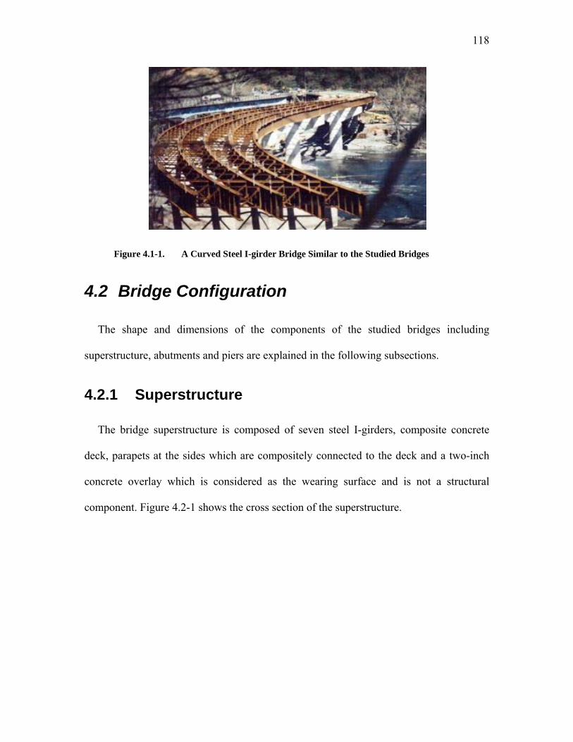
118
Figure 4.1-1. A Curved Steel I-girder Bridge Similar to the Studied Bridges
4.2 Bridge Configuration
The shape and dimensions of the components of the studied bridges including
superstructure, abutments and piers are explained in the following subsections.
4.2.1 Superstructure
The bridge superstructure is composed of seven steel I-girders, composite concrete
deck, parapets at the sides which are compositely connected to the deck and a two-inch
concrete overlay which is considered as the wearing surface and is not a structural
component. Figure 4.2-1 shows the cross section of the superstructure.

119
Figure 4.2-1. Cross Section of the Composite Steel Superstructure
The girders have two different cross sections at mid-span and over piers. Dimensions
of different girder sections are illustrated in Figure 4.2-2. As can be seen, the depth of the
web is equal to 66 inches throughout the length of the girders, but other dimensions are
different for positive and negative moment regions. The total height of the steel section is
69.5 and 70.25 inches at mid-span and over the piers, respectively. The spacing of the
girders is 9 feet. There is a concrete haunch of variable thickness between the girders and
the deck which provides a 6% superelevation over the top flange of the girders with its
variable thickness. The average thickness of the haunch is 1.5 inches over the entire
length of the girders except a length of 15 feet at each side of the piers that the thickness
reduces to 1 inch.
2" OverlayParapet Parapet
9' 9' 9' 9' 9' 9'
16" 58 ft = 696 in.
3'-4" 3'-4"
16"

120
Figure 4.2-2. Steel I-Girder Dimensions
The thickness of the concrete deck is 8 inches and its width is 60’-8”. The effective
roadway width of the bridge is 58 feet. At the two sides of the superstructure, there are
two concrete parapets which are connected to the deck using rebars. The width and height
of each parapet are 16 and 42 inches, respectively.
4.2.2 Abutments
The abutments of the modeled bridges are integrally connected to the superstructure
which is the main characteristic of this type of bridges. Each abutment is consisted of a
concrete wall with a thickness of 3’-5 13/16“ and a varying height between 9’-4” to 13’.
The wall is sitting on a row of seventeen HP12x53 steel piles with a length of 70 feet and
spacing of 3’-6”. The wing walls of the studied bridges are separated from the abutment
wall with a joint so that from a structural stand point, they are not affecting the behavior
of the bridges. Also, the approach slabs are connected to the abutment wall using a pin
joint detail. So, the only reaction force from the approach slab is a vertical load that is
8"
2"1"
66"
2.25"24"
24"
5"/8
8"
1.5"1.5"
66"
2"18"
18"
0.5"
Over PiersMid-Span

121
applied to the abutment walls and then transmitted to the steel piles and the surrounding
soil.
There are several details for connecting an abutment to bridge superstructure
integrally, which can be found in the references. For composite steel superstructures, the
integral connection can be achieved by continuing the steel girders in the concrete wall
and connecting these two elements using rebars that go through the web of the girders.
Figure 4.2-3 shows the details of such an integral connection.
Figure 4.2-3. Abutment Integral Details
4.2.3 Piers
The piers of the studied bridges consist of two hammerhead columns, a cap beam and
two pile caps each of them resting on two rows of five steel H-piles. All the components
of the piers other than the H-piles are made of reinforced concrete. The columns have a
3’-6” by 10’-9” rectangular cross section and a length of 38 feet. At the top, the width of
each column is gradually widened to 29’-9”. The cap beam which connects the columns
29 13/16"
Var. 9'-4"~13'
HP12x53
Seat Beam
12"
12"

122
to each other has a length of 59’-6”, a width of 4’-6” and a varying depth from 4’ to 7’-7”
which provides a 6% superelevation for the bridge. The pile cap of each column is a
21x7.5x4 cubic feet concrete mass which is supported on ten HP14x89 steel piles with 95
feet length. Figure 4.2-4 shows a general picture of the piers of the studied bridges.
Figure 4.2-4. Pier Configuration
The superstructure is resting on piers by means of bearings which can be either
elastomeric, sliding, fixed pot or guided pot. In the fixed pot bearings, the horizontal
movement of the superstructure and the cap beam at the point of connection is tied to
each other and the other four degrees of freedom are provided by means of an elastomeric
layer which is in the pot. These elements are modeled using nonlinear gap springs. In the
guided pot bearings, using a stainless steel PTFE plate and a shear key, the horizontal
movement is set so that it is free in one horizontal direction and fixed in the other
horizontal direction (perpendicular to the free DOF). The other four degrees of freedom

123
are provided by the elastomeric layer and are modeled by gap elements, similar to fixed
pot bearings. Figure 4.2-5 shows the springs modeling the bearings of the piers.
Figure 4.2-5. Springs Modeling the Bearings of the Piers
4.3 Finite Element Modeling
In this section, the characteristics of the finite element models of the studied curved
steel integral abutment bridges are explained. These characteristics include material
properties, loading, soil-structure interaction and the employed elements in the finite
element models.
4.3.1 Material Properties
In the studied bridges, the material for I-girders flanges and webs, braces, stiffeners
and all splices conforms to the requirements of ASTM A709/A709M, Grade 50
weathering steel. The steel material for H-piles conforms to ASTM A709, Grade 36. All
structural steel materials have a unit weight of 490 lb/ft3, a coefficient of thermal
expansion of 6.5x10E-6 /°F, a modulus of elasticity of 29000 ksi and a Poisson ratio of
0.3.

124
Other components including deck slab, parapets, abutment walls, columns, cap beams
and pile caps are reinforced concrete parts with a 28-day compressive strength equal to
4 ksi. These parts have a unit weight of 150 lb/ft3, a coefficient of thermal expansion of
6x10E-6 /°F, a modulus of elasticity of 3644 ksi and a Poisson ratio of 0.2.
4.3.2 Loading
In this section, the applied loads to the modeled bridges are reviewed. These loads
include the self weight of the bridge components, the weight of the wearing surface and
railing, the effects of live load including gravity, braking and centrifugal forces, the
pressure of soil to the abutments, the thermal loads including expansion, contraction and
temperature gradient through the thickness of superstructure and the effect of concrete
shrinkage. An explanation of each of these loads is presented in the following
subsections.
A) Dead Load (DC)
Assuming a unit weight of 150 / for the reinforced concrete components and a
unit weight of 490 / for steel components of the bridges, the dead load of the
modeled bridges is applied to all elements through calculating the volume of each
element.
B) Wearing Surface Load (DW)
Considering a 2-inch thick future concrete overlay with a unit weight of 145 / ,
the weight of wearing surface which is equal to 1.678E-4 ksi is applied to the bridges
decks. Also, the cross sectional area of each concrete side railing is assumed to be 498

125
, which results in a weight of 519 / along the edges of the bridges. A schematic
picture of the wearing surface components is shown in Figure 4.3-1.
Figure 4.3-1. Wearing Surface of the Modeled Steel Bridges
C) Earth Pressure (EH)
The pressure of the backfill soil is applied to the modeled bridges assuming a
cohesionless soil with a unit weight of 125 / and an angle of internal friction of 30
degrees. In this way, the soil pressure is:
3.617 10 5 Eq. 4.1
In which is depth of the soil layer in inches and is the soil pressure in ksi.
Elaborate explanations on how the soil pressure is applied to the structure are presented
in Section 4.3.4 (Soil-Structure Interaction).
2" Future Overlay
Parapet Parapet
108 108 108 108 108 108
16 58 ft = 696 in. 16
40 40

126
D) Live Load (LL)
Live load is applied to the models based on the AASHTO LRFD Bridge Design
Specifications (American Association of State Highway and Transportation Officials,
2010). According to the specifications four different loads should be considered for such
continuous superstructures:
- Design truck plus the lane load
- Design tandem plus the lane load
- For negative moments and piers reaction: 90 percent of dual design trucks plus the
lane load
- And again for the negative moments and piers reaction: dual tandem plus the lane
load
An impact factor of 1.33 is applied to all live loads except the lane loads. In addition, a
multiple lane presence factor is applied which is derived from Table 4.3-1.
Number of Loaded Lanes Multiplication Factor
1 1.20
2 1.00
3 0.85
> 3 0.65
Table 4.3-1. Multilane Presence Factors
The live loads are applied in the most critical place in each lane so that the maximum
effects are concluded. Figure 4.3-2 shows the positioning of the live load on the modeled
bridge decks.

127
Figure 4.3-2. Positioning of the Live Load
E) Braking Force (BR)
As per AASHTO LRFD Bridge Design Specifications, the braking force for each lane
is the maximum of 25 percent of the design truck weight or 5 percent of the design truck
plus lane load weight. This force is calculated for different bridge lengths and applied for
different positions of the live load.
It should be noted that as there are four lanes on the modeled bridges and the
simultaneous braking of the live load of all the lanes is considered, a multilane presence
factor based on Table 4.3-1 is applied to the braking forces. It should also be mentioned
that for bridges with length of less than 450 feet, the braking force of a truck which is 25
percent of its weigh is governing and this force is equal to 11.7 kips per lane:
72 0.25 0.65 11.7 /
For bridges with lengths more than 450 feet, the braking force based on truck plus lane
loading is governing which depends on the length of the bridge:
24722424247224242472242424722424120
12 ft12 ft12 ft12 ft120" < 12 ft

128
0.05 72 0.64 0.65 2.34 0.0208 /
F) Centrifugal Force (CE)
When a bridge has horizontal curvature, an important lateral load which is applied to
the bridge superstructure is the centrifugal force of the moving loads. Based on AASHTO
LRFD Bridge Design Specification 2010, this radial force is the product of the weight of
design truck or tandem and a factor defined as:
Eq. 4.2
where is equal to 4/3 for all limit states other than fatigue, is the design speed, is
the radius of curvature of the design lane and is the gravitational acceleration equal to
32.2 / . If the parameters in this equation are in a consistent set of units, the factor
will be unitless. Actually based on Eq. 1.4 and Eq. 4.2, the centrifugal force factor should
be equal to
4
3 0.28 Eq. 4.3
But for design purposes, the structural design speed may be assumed slightly more
than the geometrical design speed. Table 4.3-2 shows the values of C factor and
equivalent centrifugal forces for different radii of curvature at design speeds from 35 to
60 mph. In the calculations, a multilane presence factor of 0.65 is applied for four lanes
of loading. Note that the assumed design speeds are about 5 mph more than the speed
given by Eq. 1.4.

129
Radius of
Curvature (ft)
Geometrical
Design Speed
(mph)
Structural
Design Speed
(mph)
C Factor Centrifugal
Force (kips per
lane)
300 30.7 35 0.364 17.04
538 41.2 45 0.335 15.68
1000 56.1 60 0.324 15.16
Table 4.3-2. C Factor for Different Radii
As can be seen, the value of the C factor is almost constant ranging from 0.324 to
0.364.
G) Wind Load (WS)
The wind load is applied to the modeled bridges based on the AASHTO LRFD Bridge
Design Specification. The pressures of the wind load are assumed to be caused by a base
design wind which has a speed of 100 mph. The wind pressure has a horizontal direction
and is uniformly distributed over the areas of the bridge exposed to the wind as seen in
the elevation view.
The pressure of design wind, , is calculated using the following equation in ksf:
Eq. 4.4
in which is the base wind pressure specified in Table 4.3-3, (mph) is the design
wind velocity at design elevation and is the base wind velocity equal to 100 mph at
30.0 feet height.

130
Structural
Component
Windward Load
(ksf)
Leeward Load (ksf)
Beams 0.05 NA
Trusses, Columns
and Arches
0.05 0.25
Large Flat Surfaces 0.04 NA
Table 4.3-3. Base Wind Pressure, Corresponding to
The wind loading shall not be less than 0.30 klf on beam and girder components like
the superstructure of the bridges.
As the bridge superstructure’s elevation is more than 30 feet (the height is ranging
from 43 feet to 56.44 feet), there should be an adjustment on the as follows:
2.5 Eq. 4.5
where:
: Friction velocity taken as specified in Table 4.3-4
: Wind velocity at 30 feet above low ground or design water level assumed to be
equal to 100
: Height of the structure at which wind load are being calculated measured from low
ground or water level (> 30 feet)
: Friction length of upstream fetch taken as specified in Table 4.3-4

131
Condition Open Country Suburban City
(mph) 8.20 10.9 12.0
(ft) 0.23 3.28 8.20
Table 4.3-4. Values of and for Various Upstream Conditions
Where the wind direction is not perpendicular to the structure, the base wind pressure
shall be modified as specified in Table 4.3-5.
Skew Angle of
Wind (Degrees)
Girder Lateral Load
(ksf)
Girder Longitudinal
Load (ksf)
0 0.050 0.000
15 0.044 0.006
30 0.041 0.012
45 0.033 0.016
60 0.017 0.019
Table 4.3-5. Base Wind Pressure, for Various Angles of Attack
The forces directly applied to the substructures shall be calculated using a base wind
pressure of 0.040 ksf. Also, a vertical upward wind pressure of 0.020 ksf should be
applied to the horizontal surfaces of the bridges.
Now, using the above equations the wind pressures on the studied bridges are
calculated as follows. Assuming an open country condition for the bridge which is the
most severe case, will be 8.20 mph and will be 0.23 foot. As the average height of
the superstructure is 49.72 feet, the design wind velocity will be:
132
2.5 2.5 8.20100100
49.720.23 110.2 mph
Since for the girder structures the base wind pressure, , is 0.05 ksf, pressure of
design wind will be:
0.05 110.2100 0.0607
Therefore the forces on different elements of the modeled bridges will be:
0.0607 4.22 10 : On the vertical surface of girders and parapets
0.020 1.39 10 : On the horizontal surface of deck
0.040 2.78 10 0.01168 : On the vertical surfaces of columns
As this study is mainly focused on curved bridges and there are no unique longitudinal
and transverse directions for such bridges, especially for highly curved ones, after
choosing the direction of the wind, the pressures should be calculated and applied to the
vertical surfaces based on the different angles of attack for different parts. With a
pressure of design wind equal to 0.0607 ksf, the pressures applied to the parts in an
average height of 49.72 ft will be as presented in Table 4.3-6.

133
Skew Angle of
Wind (Degrees)
Girder Lateral Load
(ksi)
Girder Longitudinal
Load (ksi) 0 4.22 10 0.000
15 3.71 10 0.51 10
30 3.46 10 1.01 10
45 2.79 10 1.35 10
60 1.43 10 1.60 10
Table 4.3-6. Wind Pressure, for Various Angles of Attack
H) Uniform Temperature Changes (TU)
Seasonal temperature changes are applied to the modeled bridges based on the contour
maps that are given in AASHTO as the more precise method of determining the
temperature changes for each region. For a steel girder bridge composite with concrete
deck, a maximum design temperature of 120°F and a minimum design temperature of
-30°F can be a worst case scenario that can be envisioned. An assumed construction
temperature between 60°F and 70°F results in an increase of +60°F and a decrease of
-100°F for the bridge structure. These two temperature changes are applied to the
modeled bridges as the uniform temperature loading.
I) Temperature Gradient (TG)
The temperature gradient loading is applied to the modeled bridges based on the
provisions of AASSTO LRFD Specifications. Figure 4.3-3 illustrates the considered
pattern for positive gradient. Assuming a solar radiation zone “1” for the location of the
modeled bridges, the temperatures T1 and T2 are equal to 54°F and 14°F, respectively.

134
For composite steel girder bridges, the value of A is 12 inches and t is the thickness of
concrete deck. Based on these assumptions a non-uniform temperature gradient is
obtained for the concrete deck and there will be no gradient in the steel girders. The
negative temperature gradient is obtained by multiplying the values of positive gradient
by -0.30. These two gradient patterns are applied to the computer models.
Figure 4.3-3. Positive Temperature Gradient in the Superstructure Section
J) Shrinkage (SH)
To account for the effect of concrete shrinkage in the models, first the strain due to
concrete shrinkage is calculated and then the equivalent temperature decrease which
causes the same amount of strain is found. In this way, the effect of concrete shrinkage is
simulated by applying a temperature decrease to the concrete parts.
To calculate the strain in concrete due to shrinkage, the method presented by
AASHTO LRFD is used (American Association of State Highway and Transportation
Officials, 2010). In the code, the shrinkage strain is obtained using the following
equation:

135
0.48 10 Eq. 4.6
in which:
1.45 – 0.13 / 1.0
2 0.014
5
1
61 4
where:
= relative humidity (%). In the absence of better information, may be taken from
Figure 4.3-4.
= factor for the effect of the volume-to-surface ratio of the component
= factor for the effect of concrete strength
= humidity factor for shrinkage
= time development factor
= maturity of concrete (day), defined as age of concrete between the end of curing
and the time being considered for shrinkage effects
= age of concrete at time of interest (day)
/ = volume-to-surface ratio (in.)

136
= specified compressive strength of concrete at time of prestressing for pre-
tensioned members and at time of initial loading for non-prestressed members. If
concrete age at time of initial loading is unknown, may be taken as 0.80 (ksi).
AASHTO LRFD 2010 states that if the concrete is exposed to drying before 5 days of
curing have elapsed; the shrinkage strain should be increased by 20 percent.
Figure 4.3-4. Annual Average Ambient Relative Humidity in Percent
For concrete deck of the superstructure, assuming a relative humidity of 70 percent for
the location of the bridge under consideration, a / ratio equal to 4.0 inches, an of 4
ksi for superstructure concrete and a time of infinity for calculation of the time
development factor, the following values are obtained:
12 12 812 12 2 4.0

137
1.45 – 0.13 1.45 0.13 4 0.93 1.0 1.0
2 0.014 2 0.014 70 1.02
5
15
1 0.80 4 1.19
61 4 ∞
61 4 4 ∞ 1.0
For parapets the ratio and are calculated as follows:
42 12
42 12 42 5.25
1.45 – 0.13 1.45 0.13 5.25 0.77 1.0 1.0
For abutment walls the ratio and are calculated as follows:
728 158 48
728 158 158 48 2 728 48 33.4
1.45 – 0.13 1.45 0.13 33.4 2.89 1.0 1.0
And for the pier columns the ratio and are equal to:
129 42129 42 2 15.8
1.45 – 0.13 1.45 0.13 15.8 0.60 1.0 1.0
The other coefficients including , , are the same as those of deck and so the
shrinkage strain can be calculated as:

138
1.0 1.02 1.19 1.0 0.48 10 583 10
Now, the equivalent temperature decrease can be evaluated using the following
equation:
∆
Hence:
6 10 ∆ 583 10
∆ 97.2 °
The effect of shrinkage of the concrete deck, parapets, abutment wall and pier columns
is applied to the modeled bridges by assuming a contraction of -97.2°F for these parts. In
this case of loading, there is no temperature change in the other elements of the bridge.
4.3.3 Load Combinations
The load combinations used for studied bridges are based on Table 3.4.1-1 of
AASHTO LRFD. In general, a factored load effect can be taken as:
Eq. 4.7
in which ’s are load modifiers that are taken equal to unity, ’s are the load factors
from Table 3.4.1-1 of AASHTO LRFD and ’s are the load effects. Among all the
possible load combinations given in Eq. 4.7, some of them realized to be critical for the
studied bridges that are discussed as follows.
For Strength I Limit State, Eq. 4.7 results in:

139
, 1.75 1.75 1.75
0.5 1.2 0.5 1.2 Eq. 4.8
Where
, 1.25 0.90
, 1.5 0.65
, 1.35 0.90
The possible rational load combinations comes from maximizing or minimizing
, maximizing or minimizing , maximizing or minimizing . The
following eight load combinations are the final result from Eq. 4.8.
, 1.25 1.5 0.9 0.65 1.35 0.9
1.75 1.75 1.75 0.5 1.2
Eq. 4.9
For the term , it is observed that contraction and shrinkage act in the same
direction, while expansion is opposite to shrinkage. Therefore, a more simplification is to
take 1.2 0.5 and 1.2 1.2 . However, the more general expression
arises less questions about the possible critical combinations.
For Strength III Limit State, Eq. 4.7 yields:
, 1.25 1.5 0.9 0.65 1.35 0.9
1.4 0.5 1.2 Eq. 4.10
In addition to strength limit states, the bridges are also studied in service limit states.
Eq. 4.7 gives the following Service I Limit State combinations:

140
, 1.0 1.0 1.0 1.0 1.0 1.0
0.3 1.0 0.5 1.2 Eq. 4.11
In which is equal to 0.5 for the load combinations that have live load included and
equal to 1.0 when live load is not considered. These load combinations are regarded in
this study on the integral bridges.
4.3.4 Soil-Structure Interaction
This section presents detailed explanation on the employed methods for calculation of
the interaction forces between the elements of the modeled bridges and the adjacent soil.
Based on theories of soil mechanics, the soil pressure depends on the magnitude and
direction of the structure displacement. If the structure is pushed against soil, the pressure
changes nonlinearly between at-rest and passive pressure. And if the structure is moving
away from neighboring soil, the interaction pressure decreases nonlinearly from at-rest to
active soil pressures, depending on the magnitude of the movement. To predict these
nonlinear responses, there are some available methods in literature which will be used in
the finite element models.
As the soil exists all around the piles of abutments or piers, but in the case of abutment
walls, the soil is just in one side of the wall, there are two different soil pressure response
curves for these two cases which will be explained separately in the following
subsections.

141
A) Soil-Abutment interaction
In soil mechanics, lateral soil pressure is generally defined as a ratio of vertical earth
pressure. This ratio that is known as the earth pressure coefficient is a variable that
changes based on the state of interest which can be active, at-rest, passive or something
between. For a wall supported laterally by soil, Clough G. W. and Duncan J. M. have
performed a series of finite element analyses to perceive the soil behavior (Clough,
Duncan, University of California, & Dept. of Civil Engineering, 1971). They developed a
relationship between the wall movement and the soil pressure which is shown in
Figure 4.3-5. As can be observed the soil pressure changes from passive pressure to
active pressure based on the direction and magnitude of the wall displacement. In the
present study, the curve that they have presented for an internal friction angle of 30
degrees is entered as the response curve into the finite element models.
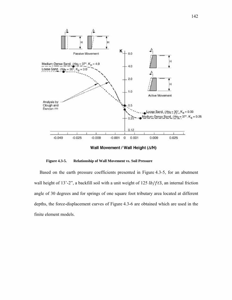
142
Figure 4.3-5. Relationship of Wall Movement vs. Soil Pressure
Based on the earth pressure coefficients presented in Figure 4.3-5, for an abutment
wall height of 13’-2”, a backfill soil with a unit weight of 125 / 3, an internal friction
angle of 30 degrees and for springs of one square foot tributary area located at different
depths, the force-displacement curves of Figure 4.3-6 are obtained which are used in the
finite element models.

143
Figure 4.3-6. Force-Displacement Curves of the Abutment Backfill Springs
As the backfill of the bridge abutments are generally composed of granular soils, the
response curve for abutment springs is only presented for cohesionless soils and therefore
cohesive soil behavior for abutment backfill is ignored.
B) Soil-Pile Interaction
The response of the soil interacting with piles of piers or abutments is different than
that for abutment walls because the piles are fully embedded in soil or in other words the
soil completely surrounds the piles. So the pile movement in all directions results in
pushing a mass of soil. In this way, if one wants to study this problem in 2D, for each
point of the pile if the pile is not moving, the at-rest pressures of the two sides are equal
and the total pressure on the pile is equal to zero. And if the pile moves in a direction, the
value of the soil pressure is equal to the pressure value resulted from a displacement of
the same magnitude but in the opposite direction. This 2D reasoning is valid for all
horizontal directions in a 3D space and therefore displacement versus pressure curves that
‐2.00
‐1.00
0.00
1.00
2.00
3.00
4.00
5.00
6.00
‐10.00 ‐8.00 ‐6.00 ‐4.00 ‐2.00 0.00 2.00 4.00 6.00
Force (kip)
Displacement (in.)
Force‐Displacement Curve for Abutments Springs
Depth=158"
Depth=118"
Depth=79"
Depth=39"

144
are presented by the researchers is skew-symmetrical with respect to zero pile
displacement.
One of the sources for solution of this problem is the recommendations of American
Petroleum Institute which proposes soil response curves for both cohesive and
cohesionless soils (American Petroleum Institute, 2005). The following subsections
describe the API recommendations.
B1) Lateral Load-Deflection in Soft Clay
The response of soft clay under lateral loading is generally a nonlinear behavior. API
proposes a p-y curve for short term static loading which may be generated from
Table 4.3-7.
/ /
0 0
0.23 0.1
0.33 0.3
0.5 1
0.72 3
0.98 8
1 ∞
Table 4.3-7. Proposed API p-y Curve for Soft Clay
in which:
: actual lateral pressure

145
: lateral bearing capacity of soft clay
: actual lateral deflection
2.5 .
: strain which occurs at one half of the maximum stress on laboratory unconsolidated
undrained compression tests of undisturbed soil samples
: pile diameter
The lateral bearing capacity of soft clay has been found to be between 8 and 12
except at shallow depths which failure mode changes due to lack of enough overburden
pressure. In the present study, this capacity is assumed to be equal to 9c for deep
elements of the pile and for shallower positions, i.e. at depth smaller than reduced
resistance zone ( ), it is linearly increased between 3 and 9 :
3
9
Eq. 4.12
: undrained shear strength for undisturbed clay samples
: effective unit weight of soil
J: a dimensionless empirical constant with values ranging from 0.25 to 0.5
X: depth below soil surface
: depth below soil surface to bottom of reduced resistance zone. For constant soil
strength with depth:

146
6
Based on the above mentioned equations, the force-displacement curves for the
springs of abutment piles are obtained which are plotted in Figure 4.3-7. These graphs
correspond to the response for HP12x53 piles with spring spacing of 5 feet, soil unit
weight of 125 lb/ft3, undrained cohesion of 2 ksf, J value of 0.4 and equal to 0.01.
Figure 4.3-7. Force-Displacement Curves of the Springs of Piles of Abutments in Soft Clay
Also for piles of piers with HP14x89 sections, for springs of five feet spacing and the
same soil properties and same J and values, the force-displacement curves of
Figure 4.3-8 are found.
‐100
‐80
‐60
‐40
‐20
0
20
40
60
80
100
‐6 ‐4 ‐2 0 2 4 6Force (kip)
Displacement (in.)
Force‐Displacement of Abutment Pile Springs
Depth>12.78 ft
Depth=10 ft
Depth=5 ft

147
Figure 4.3-8. Force-Displacement Curves of the Springs of Piles of Piers in Soft Clay
B2) Lateral Load-Deflection in Sand
API recommends a hyperbolic tangent equation for the lateral force-displacement
curve of the piles in sand as follows:
. . . tanh
Eq. 4.13
Where:
: Lateral soil resistance in a length of of pile (force)
: An empirical correction factor, 3 0.8 0.9
: Estimated ultimate lateral soil resistance (force/unit length)
: Length of the pile section
: Initial modulus of subgrade reaction from Figure 4.3-9
‐150
‐100
‐50
0
50
100
150
‐6 ‐4 ‐2 0 2 4 6Force (kip)
Displacement (in.)
Force‐Displacement of Pier Pile Springs
Depth>14.62 ft
Depth=10 ft
Depth=5 ft

148
: Depth from the top of the soil layer
: Displacement in the horizontal direction
Figure 4.3-9. Initial Modulus of Subgrade Reaction
The ultimate soil lateral resistance can be obtained based on the equations given in
API recommendations as the minimum of:
. . Eq. 4.14
And
. . . Eq. 4.15

149
where:
: Ultimate sand lateral resistance at shallow depths (force/unit length)
: Ultimate sand lateral resistance at deep depths (force/unit length)
: Pile Diameter
: Effective soil density
: Angle of internal friction
45
1
/2
45
: Active earth pressure coefficient
: At-rest earth pressure coefficient
The values of constants , and can be found from Figure 4.3-10. This figure
may also be used to check the values obtained from the relevant equations.

150
Figure 4.3-10. Values of Coefficients , and as a Function of Angle of Friction
Using the above equations and considering a width of 13.8 inches for HP14x89 piles
of piers, a soil unit net weight of 125 / , an angle of internal friction of 30 degrees and
a one foot spacing for the pile springs, a k value of 45 lb/in3 is obtained from Figure 4.3-
9, which results in the force-displacement curves of Figure 4.3-11 for the pile springs. As
shown in these two graphs, the force-displacement curves strongly depend on the depth
of the springs.

151
Figure 4.3-11. Force-Displacement Curves of the Springs of Piles of Piers in Sand
The response of the springs of the HP12x53 piles of the abutments can be plotted by
employing the same values as used for the pier piles in the related equations and
considering a width of 11.8 inches for the piles. Figure 4.3-12 shows the force-
displacement curves for these springs.
‐2000
‐1500
‐1000
‐500
0
500
1000
1500
2000
‐4 ‐3 ‐2 ‐1 0 1 2 3 4
Force (kip)
Displacement (in.)
Force‐Displacement of Pier Pile Springs
Depth=19 ft
Depth=38 ft
Depth=57 ft
Depth=76 ft
Depth=95 ft
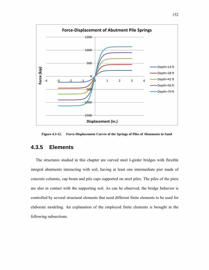
152
Figure 4.3-12. Force-Displacement Curves of the Springs of Piles of Abutments in Sand
4.3.5 Elements
The structures studied in this chapter are curved steel I-girder bridges with flexible
integral abutments interacting with soil, having at least one intermediate pier made of
concrete columns, cap beam and pile caps supported on steel piles. The piles of the piers
are also in contact with the supporting soil. As can be observed, the bridge behavior is
controlled by several structural elements that need different finite elements to be used for
elaborate modeling. An explanation of the employed finite elements is brought in the
following subsections.
‐1500
‐1000
‐500
0
500
1000
1500
‐4 ‐3 ‐2 ‐1 0 1 2 3 4
Force (kip)
Displacement (in.)
Force‐Displacement of Abutment Pile Springs
Depth=14 ft
Depth=28 ft
Depth=42 ft
Depth=56 ft
Depth=70 ft
153
A) Beam Element
To model the superstructure braces, pier columns, cap beams and also the piles of the
piers and abutments, two-node frame elements are used. The frame elements have a
general three dimensional beam column formulation. In these elements the effects of
axial deformation, biaxial bending, torsion and biaxial shear can be modeled. A frame
element is a straight line between two points. Each element has its own local coordinate
system for assigning element properties and loads. Another characteristic of these
elements is end offset which enables one to more accurately model the intersection of two
elements, such as intersection of the columns of these bridges with the relatively rigid
pile caps. The rigidity of end offsets can vary by setting a parameter called rigid zone
factor to model partial to full rigidity. These elements can be loaded by gravity, multiple
concentrated loads, multiple distributed loads, temperature induced loads and strain and
deformation loads.
B) Shell Element
Several parts of the modeled bridges including the deck slab, parapets, flanges and
webs of the I-girders, stiffeners, abutment walls and pile caps are modeled using shell
elements. A shell element is a three- or four-node formulation which combines
membrane and plate behaviors.
For defining material properties and loads and for getting output, each shell element
has its local axes. Different types of loadings are possible in these elements including
gravity and uniform loads, surface pressure on the side faces and also the top, bottom

154
surfaces and temperature loads. In these elements temperature-dependent, orthotropic
material properties can also be defined.
Shell elements use a four-point numerical integration formulation. Stresses and
internal forces and moments are calculated at the 2-by-2 Gauss integration points and
then extrapolated to the joints of the element. From the difference in values of stresses or
internal forces calculated from different elements attached to a common joint, an estimate
error in the solution can be approximated. This is an indication of the accuracy of a given
finite-element meshing and can then be used as the basis for optimizing the mesh for a
new and more accurate solution.
C) Nonlinear Link Element
Nonlinear link elements are used to connect two joints together with specified
nonlinear properties. Each link element may show up to three types of behavior based on
the required properties and the analysis type. These properties include: linear, nonlinear
and frequency-dependent.
In the modeled bridges, these link elements are used to simulate the elastomeric
bearings connecting the piers to the superstructure. The properties assigned to these link
elements are described here. In design of the elastomeric bearings, it is assumed that the
area of the bearing should be chosen so that the pressure on the elastomeric bearing is not
less than a specified value, namely one third or one fourth of the maximum allowed
pressure on the bearing. This assumption yields to the fact that these types of bearings
shall not in tension in any of the load combinations. On the other hand, as the maximum
applied pressure on the elastomer is limited by the manufacturers (typically to 2 ksi), the

155
stiffness of the link element in the six degrees of freedom can be determined using the
following equations. In these equations, the gravity direction of the neoprene is assumed
as direction 1 and the two horizontal directions are named 2 and 3. The elastomers are
circular with radius of 14 inches and have a thickness of 4 inches. The modulus of
elasticity of elastomeric material is 85.3 ksi and it has a shear modulus of elasticity of
0.142 ksi.
Axial stiffness:
6565 /
Shearing stiffness:
10.9 /
Torsional stiffness:
268 . /
Bending stiffness:
80 427 . /
Where:
is the cross sectional area, is axial modulus of elasticity, is the rubber thickness,
is the shear modulus of elasticity, is the torsional constant (equal to for circular
elastomers) and is the moment of inertia of the section of the elastomeric bearing.

156
In this way, six stiffnesses of the bearings are calculated and entered into the finite
element model. A picture of the bearing springs modeled in a pier is shown in Figure 4.3-
13.
Figure 4.3-13. Modeling of the Bearings
Later in this study, the effects of fixed and guided pot bearings are also examined. For
those types of bearings, if the elastomeric layer of the pot is assumed to have a circular
shape with the radius of 18 inches and thickness of 1 inch, then the stiffness in the six
degrees of freedom will be calculated as follows:
Axial stiffness:
. /
21 700 /
Shearing stiffness (for fixed pots):
∞
Shearing stiffness (for guided pots in the guided direction):
0
Shearing stiffness (for guided pots perpendicular to guided direction):
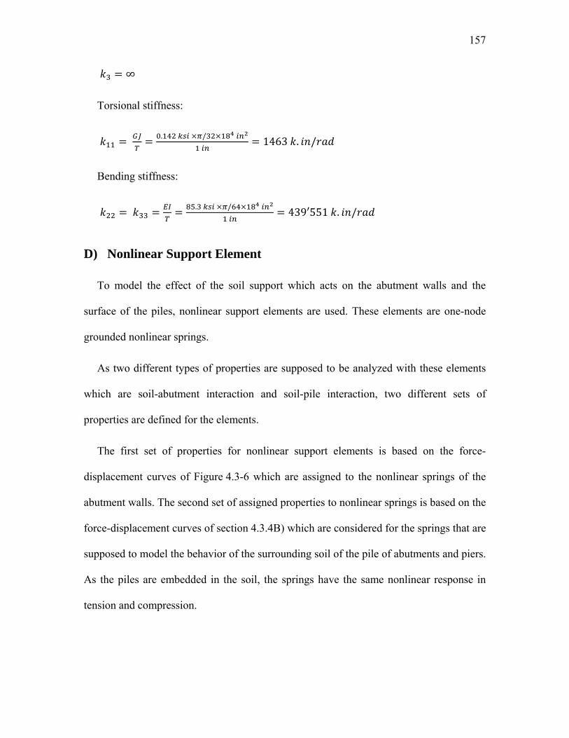
157
∞
Torsional stiffness:
. /
1463 . /
Bending stiffness:
. /
439 551 . /
D) Nonlinear Support Element
To model the effect of the soil support which acts on the abutment walls and the
surface of the piles, nonlinear support elements are used. These elements are one-node
grounded nonlinear springs.
As two different types of properties are supposed to be analyzed with these elements
which are soil-abutment interaction and soil-pile interaction, two different sets of
properties are defined for the elements.
The first set of properties for nonlinear support elements is based on the force-
displacement curves of Figure 4.3-6 which are assigned to the nonlinear springs of the
abutment walls. The second set of assigned properties to nonlinear springs is based on the
force-displacement curves of section 4.3.4B) which are considered for the springs that are
supposed to model the behavior of the surrounding soil of the pile of abutments and piers.
As the piles are embedded in the soil, the springs have the same nonlinear response in
tension and compression.

158
4.3.6 Finite Element Models
Based on the information provided in the previous sections, a comprehensive finite
element analysis study is conducted using the Nonlinear Finite Element Analysis
Program SAP 2000. In the analyses, the movements and internal forces of curved integral
abutment bridges are evaluated and compared to the responses of straight bridges.
In order to conduct such analyses, several finite element models of curved I-girder
steel bridges with radius of curvature equal to 300, 538 and 1000 feet are analyzed. For
each of these radii, the bridge is modeled in different lengths, namely; 308, 501, 694 and
887 feet. Additionally, the equivalent straight bridge of each curved model is simulated
with exact same characteristics as the curved bridge except the curvature. The span length
in the modeled bridges is 154 feet for the end spans and 193 feet for the middle spans. As
shown before, the width of all the bridges is 60’-8”. Figure 4.3-14 illustrates typical
models that are made in this study.

159
Figure 4.3-14. Typical Finite Element Models of the Studied Bridges
4.4 Results of FE Analysis
In this section, the results of the conducted finite element analyses are presented. In
the analyses, different aspects of the behavior of steel I-girder integral abutment bridges
are studied. These studies include:
- Effect of Length and Curvature on Load Responses:
A diverse set of loads are applied to the modeled bridges. The effect of bridge
curvature and bridge length on the response of different elements under each load
160
is examined. As the critical forces in an element are determined based on factored
load, the loads are combined based on the load combinations of Section 4.3.3 and
the effect of length and curvature is also presented for the envelope of load
combination effects.
- Bridge Movement:
First, it is tried to distinguish the different parameters affecting the bridge end
displacement. It is observed that the maximum bridge end displacement occurs due
to contraction and shrinkage. The reduction of the bridge length (or bridge
shortening) due to these effects is calculated. In the case of long straight bridges,
the summation of end displacements is equal to the bridge shortening. But, in
curved bridges end displacements are a function of bridge shortening. A
geometrical relationship is presented between shortening and displacement in
curved bridges. The effect of bridge width is also included.
- Abutment Pile Orientation:
The orientation of abutment piles is a problem that is studied in deep for steel
bridges. Researchers have two different opinions regarding the pile orientation.
Some believe the piles should be oriented for strong axis bending. Some others
prefer a weak axis bending. An analytical solution for this problem is presented for
the case of straight bridges. For curved bridges, several finite element analyses for
different bridge configurations are performed. Based on the results, a general
solution to find the optimum pile orientation is presented.
- Effect of Bearing Type and Orientation:

161
First, different bearing types used in bridge industry are surveyed. The different
types that are found are categorized based on their structural performance. The
effect of elastomeric, fixed, guided and sliding bearings on the internal forces of
the studied bridges is investigated. And the final recommendations on the bearing
orientation are provided.
In the following sections, all of the above-mentioned problems are developed
elaborately.
4.4.1 Effects of Length and Curvature on Load
Responses
In this section, the effect of different loads on the responses of the studied integral
abutment bridges is displayed. The piers of the bridges are isolated from the
superstructure by means of elastomeric bearings. The loads and load effects that are
considered include the self weight of the bridge, the weight of superstructure, live load,
braking force, centrifugal force, horizontal earth pressure, expansion, contraction,
positive and negative temperature gradient and finally concrete shrinkage. Since the
studied bridges are composed of several elements, the examined elements should be
limited to those elements that are the most critical from the design standpoint. The other
factor is the inspected output. As each element has a number of different outputs such as
axial or in-plane forces and also bending moments and shear forces in different
directions, the study should be narrowed down to a number of the most influential output
types.

162
With the above introduction, since the abutment piles are the most critical elements in
design of integral bridges, they are chosen for the study. For those elements, the resultant
bending moment and shear force are investigated as the desired output types. The
following subsections show the results of the finite element studies on these element
outputs.
The other problem is the magnitude of the internal forces in each element due to each
load. It should be noticed that the responses are totally different in a manner that the
responses under some of the loads are tens of times of the response due to some other
loads. So, all loads should not be considered of the same effectiveness. A weight function
is defined for each response of the elements which shows the significance of that type of
loading for that set of elements. The definition of the weight function is as below:
For example the weight function for dead load moment of pile of abutments is:
And then the average of the internal force ratios is calculated for different bridge as follows:
And the normalized weight factor for each load case is obtained using the following equation:
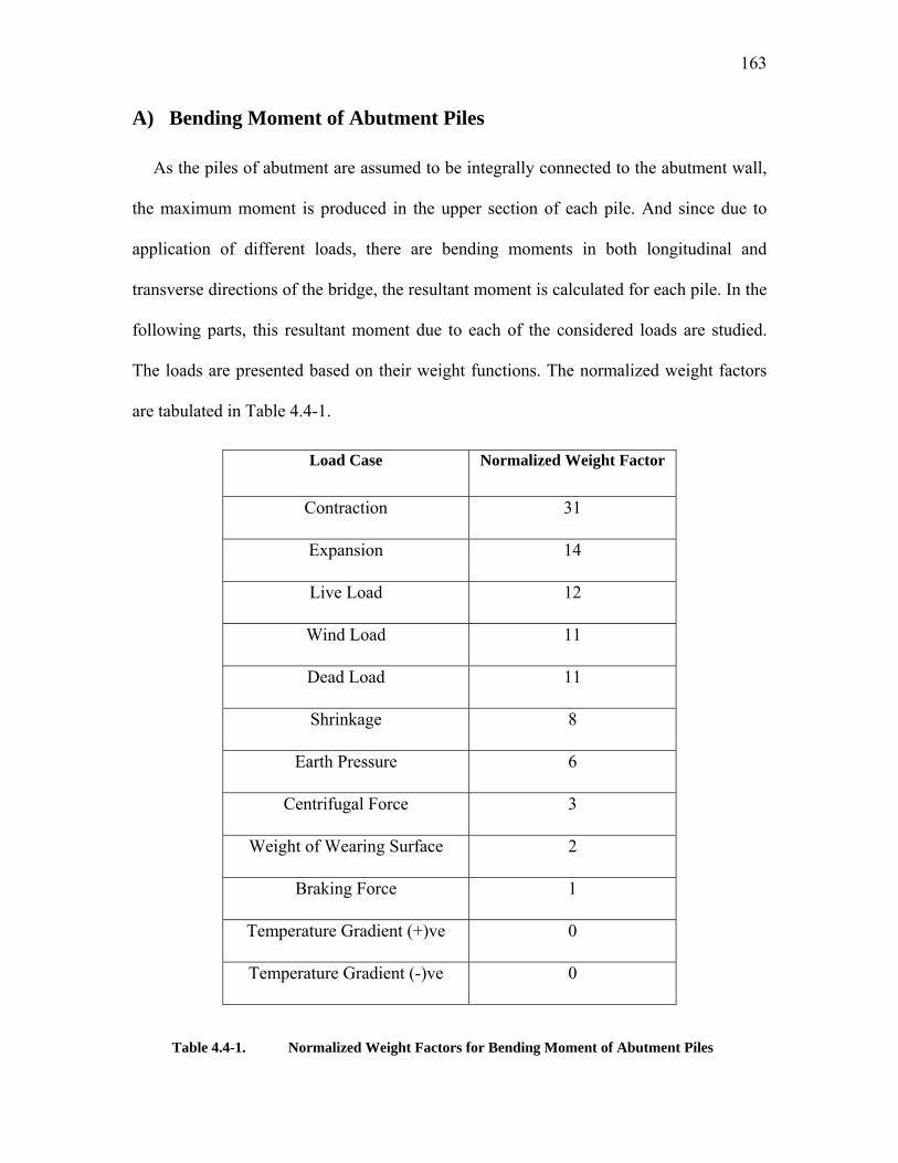
163
A) Bending Moment of Abutment Piles
As the piles of abutment are assumed to be integrally connected to the abutment wall,
the maximum moment is produced in the upper section of each pile. And since due to
application of different loads, there are bending moments in both longitudinal and
transverse directions of the bridge, the resultant moment is calculated for each pile. In the
following parts, this resultant moment due to each of the considered loads are studied.
The loads are presented based on their weight functions. The normalized weight factors
are tabulated in Table 4.4-1.
Load Case Normalized Weight Factor
Contraction 31
Expansion 14
Live Load 12
Wind Load 11
Dead Load 11
Shrinkage 8
Earth Pressure 6
Centrifugal Force 3
Weight of Wearing Surface 2
Braking Force 1
Temperature Gradient (+)ve 0
Temperature Gradient (-)ve 0
Table 4.4-1. Normalized Weight Factors for Bending Moment of Abutment Piles

164
The fact that should be mentioned about these weight factors is that these factors are
not the percentage of participation of the load compared to other loads in a load
combination. These factors show the relative magnitude of the moments due to different
load. For example, in some bridges factored contraction moment can be about 95 percent
of the critical load combinations moment, while its normalized weight factor is 31.
A1) Contraction
Contraction with a normalized weight factor of 31 is the most effective loading for the
studied bridges. In straight bridges, contraction moments in abutment piles have an
increasing trend with increase of bridge length. Figure 4.4-1 shows the curves of moment
versus length for different radii. In curved bridges with large radius of curvature, i.e.
radius of 1000 feet, the moments due to contraction tend to increase as the length
increases, but the increase is not as strict as the case of straight bridges. For bridges with
radius of 300 and 538 feet, the moment increases up to length of about 500 to 600 feet,
then it starts to decrease for longer bridges.

165
Figure 4.4-1. Maximum Moment in Abutment Piles Due to Contraction
To have a better understanding of how the moments reduce for long bridges, the
moments in piles of bridges of different radii are divided by the moment of the straight
bridge of the same length. In this way, a set of Normalized moments are calculated which
are plotted in Figure 4.4-2.
0
500
1000
1500
2000
2500
3000
3500
4000
4500
300 400 500 600 700 800 900
Mom
ent (k.in)
Bridge Length (ft)
Abutments: Integral ‐ Piers Bearing Type: Elastomeric
R=infinity
R=1000'
R=538'
R=300'

166
Figure 4.4-2. Normalized Moment in Abutment Piles Due to Contraction
As can be observed from the above graph, the pile moments in a bridge with R=300’
and L=887’ is about 17 percent of the pile moment in a straight bridge of the same length.
This shows that the abutment pile moments due to contraction not only do not necessarily
increase as the bridge length increases but also they may be reduced considerably for
long bridges.
A2) Expansion
Expansion is the second load that is studied because it has the second greatest weight
factor. The bending moment in abutment piles of straight bridges show a strictly
increasing trend as the length of the bridge increases. But in curved bridges, the moments
of the abutment piles get larger values due to increase in the length of short bridges. But
beyond a specific length which depends of the radius of curvature, the moments start to
0.00
0.20
0.40
0.60
0.80
1.00
1.20
300 400 500 600 700 800 900
Mom
ent R
atio
Bridge Length (ft)
Ratio of Maximum Moments in Abutment Piles(M curved / M straight)
Abutments: Integral ‐ Piers Bearing Type: Elastomeric
R=infinity'
R=1000'
R=538'
R=300'

167
drop off. The other noticeable point is that the values of pile moments in expansion are
considerably lower than those due to contraction. There are two reasons for this
difference. The first one is the magnitude of the considered temperature changes. The
temperature increase is +60°F while the temperature decrease is -100°F. The other reason
for lower moments compared to contraction is the soil resistance. When bridge expands,
the abutment walls are pushed against the backfill soil, and soil tries to decrease the
movement of bridge ends. That’s why in a straight bridge with L=887 feet, the pile
moment due to expansion is about 1100 k.in and that moment caused by contraction is
about 3800 k.in.
Figure 4.4-3. Maximum Moment in Abutment Piles Due to Expansion
In order to have a better view of the relative values of the moments of the studied
bridges due to expansion, a normalized graph of the curves is presented in Figure 4.4-4.
0
200
400
600
800
1000
1200
1400
300 400 500 600 700 800 900
Mom
ent (k.in)
Bridge Length (ft)
Abutments: Integral ‐ Bearing Type: Elastomeric
R=infinity
R=1000'
R=538'
R=300'

168
Figure 4.4-4. Normalized Moment in Abutment Piles Due to Expansion
The observable fact from Figure 4.4-4 is that the magnitude of abutment pile
expansion moments in a long curved bridge (L=887 feet) with a radius of 300 feet is less
than 40 percent of that of a straight bridge. In shorter bridges, the pile moments of curved
bridges are greater than those of straight bridges. The reason of larger moments in shorter
curved bridges is the lateral displacement of the abutment wall due to bridge expansion
which bends the piles about their strong axes and causes large moment in piles. In the
case of straight bridges, because of symmetry there is not large lateral displacement due
to expansion.
A3) Live Load
In the table of weight factors live load is in the third place which shows the relatively
high values of internal moments developed by live load in the abutment piles. As can be
0.00
0.20
0.40
0.60
0.80
1.00
1.20
1.40
1.60
1.80
2.00
300 400 500 600 700 800 900
Normalized
Mom
ent
Bridge Length (ft)
Ratio of Maximum Moments in Abutment Piles(M curved / M straight)
Abutments: Integral ‐ Piers Bearing Type: Elastomeric
R=infinity'
R=1000'
R=538'
R=300'
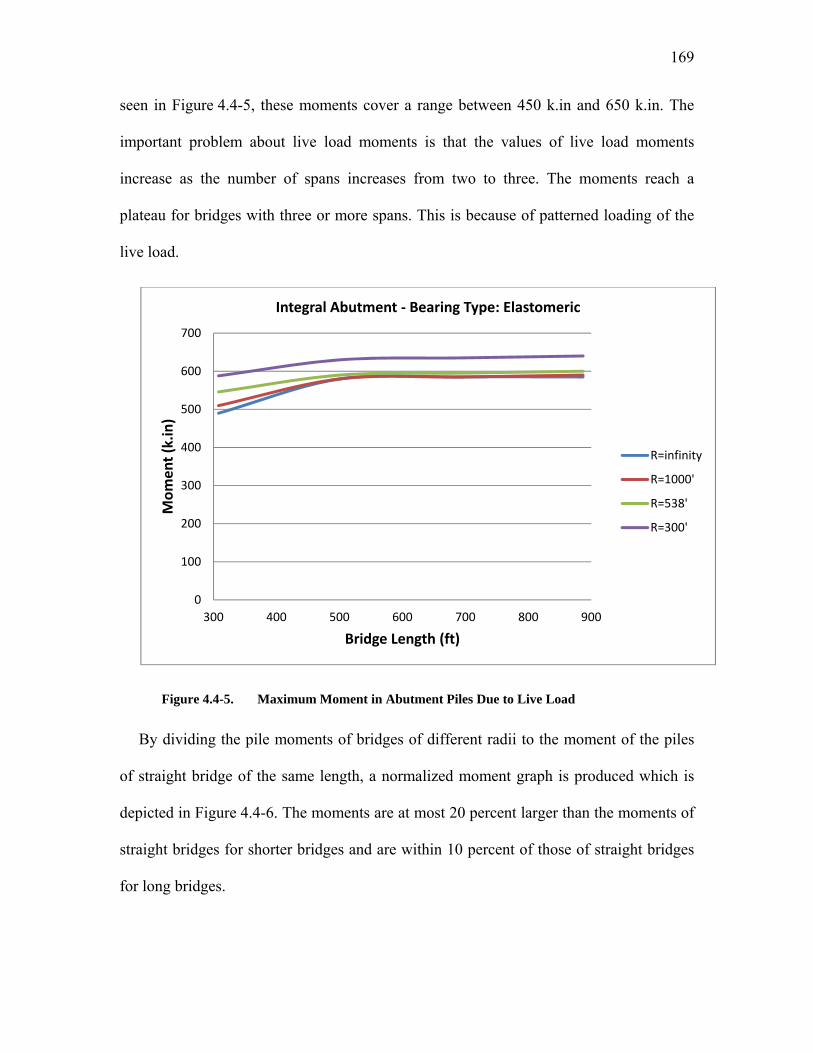
169
seen in Figure 4.4-5, these moments cover a range between 450 k.in and 650 k.in. The
important problem about live load moments is that the values of live load moments
increase as the number of spans increases from two to three. The moments reach a
plateau for bridges with three or more spans. This is because of patterned loading of the
live load.
Figure 4.4-5. Maximum Moment in Abutment Piles Due to Live Load
By dividing the pile moments of bridges of different radii to the moment of the piles
of straight bridge of the same length, a normalized moment graph is produced which is
depicted in Figure 4.4-6. The moments are at most 20 percent larger than the moments of
straight bridges for shorter bridges and are within 10 percent of those of straight bridges
for long bridges.
0
100
200
300
400
500
600
700
300 400 500 600 700 800 900
Mom
ent (k.in)
Bridge Length (ft)
Integral Abutment ‐ Bearing Type: Elastomeric
R=infinity
R=1000'
R=538'
R=300'

170
Figure 4.4-6. Normalized Moment in Abutment Piles Due to Live Load
A4) Wind Load
Lateral load transfer mechanism in integral abutment bridges is totally different than
that of jointed bridges. That’s why wind load has such a high weight factor in integral
bridges. As the piers of the studied bridges are assumed to be connected to the
superstructure by means of elastomeric bearings, and the abutments are integrally
connected to the superstructure, the larger stiffness of the abutments absorbs almost all
the lateral loads applied to the bridge. This problem is more magnified when the length of
the bridge increases. As shown in Figure 4.4-7, the moments in the abutment piles of
bridges of L=300 feet have a maximum of about 400 k.in and for length of about 900
feet, the maximum is about 900 k.in. This could lead to high stresses in the piles if there
were live load and centrifugal force on the bridge simultaneously. But the load
0.00
0.20
0.40
0.60
0.80
1.00
1.20
1.40
300 400 500 600 700 800 900
Normalized
Mom
ent
Bridge Length (ft)
Ratio of Maximum Moments in Abutment Piles(M curved / M straight)
Integral Abutment ‐ Piers Bearing Type: Elastomeric
R=infinity
R=1000'
R=538'
R=300'

171
combinations that include stormy conditions assume no live load on the bridge. Because
of this approach, which is reasonable, wind load is not a terribly critical load case on
integral abutment bridge. However, the current studies show that the wind load
combinations should always be considered for abutment piles.
Figure 4.4-7. Maximum Moment in Abutment Piles Due to Wind Load
A graph of the ratio of the moments of curved bridges to the moment of the straight
bridge of the same length is shown in Figure 4.4-8. These ratios have a maximum of
about 1.5 for shorter bridges and a maximum of 2 for longer bridges which shows the
vulnerability of curved bridges to wind load. It’s because the wind major effect on the
abutment of straight bridges is in lateral direction and the abutment stiffness in lateral
direction is much larger than the stiffness in longitudinal direction. Wind can have a
0
100
200
300
400
500
600
700
800
900
1000
300 400 500 600 700 800 900
Mom
ent (k.in)
Bridge Length (ft)
Integral Abutment ‐ Bearing Type: Elastomeric
R=infinity
R=1000'
R=538'
R=300'

172
major component in the longitudinal direction of curved bridges which causes larger
displacement and so larger moments in the abutment piles.
Figure 4.4-8. Normalized Moment in Abutment Piles Due to Wind Load
A5) Dead Load
Dead load effect on the abutment of bridges depends on the sequence of the
construction. Based on the stages that a bridge is constructed, the internal forces in the
components can be totally different. In a bridge which most of the end span is covered by
the elements cantilevered to piers, the dead load effects on the abutment are minimal at
the end of construction. But in a bridge with a large number of temporary supports that
are removed at the end of construction, the forces in the abutment can be much larger. In
the studied bridges, the dead weight of the bridge is applied to the models in a single
stage which simulates the second example with temporary supports. The shapes of the
0.00
0.50
1.00
1.50
2.00
2.50
300 400 500 600 700 800 900
Normalized
Mom
ent
Bridge Length (ft)
Ratio of Maximum Moments in Abutment Piles(M curved / M straight)
Abutments: Integral ‐ Piers Bearing Type: Elastomeric
R=infinity'
R=1000'
R=538'
R=300'

173
curves of the piles dead load moments versus bridge length are illustrated in Figure 4.4-9.
It shows that the moments decrease as the bridge length increases.
Figure 4.4-9. Maximum Moment in Abutment Piles Due to Dead Load
The magnitude of dead load moment reduction can be seen in Figure 4.4-10. The
maximum decrease is for the bridge with the smallest radius which decreases from 1.3
times of equivalent straight bridge moment to about 0.9 times of that.
0
100
200
300
400
500
600
700
800
300 400 500 600 700 800 900
Mom
ent (k.in)
Bridge Length (ft)
abutments: Integral ‐ Bearing Type: Elastomeric
R=infinity
R=1000'
R=538'
R=300'

174
Figure 4.4-10. Normalized Moment in Abutment Piles Due to Dead Load
A6) Concrete Shrinkage
In the literature related to structural effects of concrete deck shrinkage in composite
steel bridges, this phenomenon is regarded as a secondary effect in bridge structures. But
in the studied bridges, concrete shrinkage showed a noticeable effect on the abutment
piles. It can be observed from Figure 4.4-11 that shrinkage can cause moments up to
about 1100 k.in in the abutment piles of straight bridges which is a large moment. This
behavior is seen, but not of the same severity, in bridges with a radius of 1000 feet. But in
bridges with a radius of 300 or 538 feet, the pile moments are not increasing for bridges
longer than 500 or 600 feet. In these bridges, a maximum moment of about 660 k.in is
read which shows the better performance of highly curved bridges under shrinkage load
effects.
0.00
0.20
0.40
0.60
0.80
1.00
1.20
1.40
300 400 500 600 700 800 900
Normalized
: Mom
ent
Bridge Length (ft)
Ratio of Maximum Moments in Abutment Piles(M curved / M straight)
Abutments: Integral ‐ Piers Bearing Type: Elastomeric
R=infinity'
R=1000'
R=538'
R=300'

175
Figure 4.4-11. Maximum Moment in Abutment Piles Due to Concrete Shrinkage
The pattern of changes of moments versus length for different radii shows that for
shorter bridges shrinkage creates larger moments compared to straight bridges. But, as
illustrated in Figure 4.4-12, in longer bridges (L=887’), shrinkage moments are less than
70 percent of those of straight bridges.
0
200
400
600
800
1000
1200
300 400 500 600 700 800 900
Mom
ent (k.in)
Bridge Length (ft)
Abutments: Integral ‐ Bearing Type: Elastomeric
R=infinity
R=1000'
R=538'
R=300'
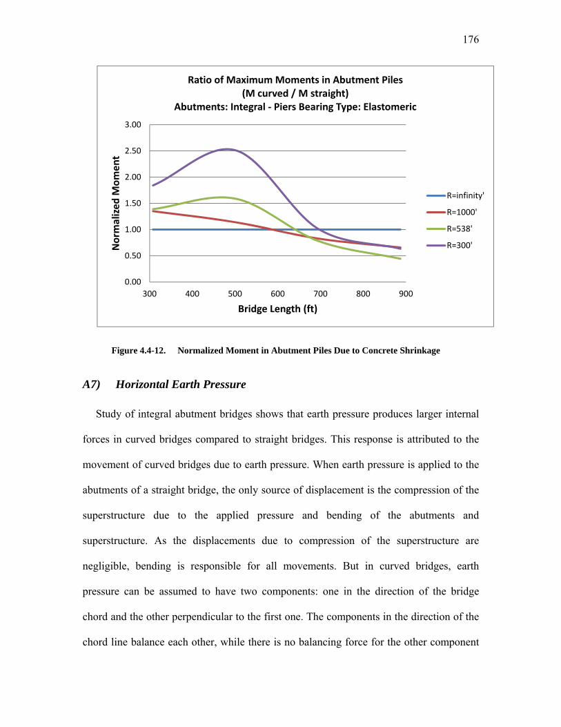
176
Figure 4.4-12. Normalized Moment in Abutment Piles Due to Concrete Shrinkage
A7) Horizontal Earth Pressure
Study of integral abutment bridges shows that earth pressure produces larger internal
forces in curved bridges compared to straight bridges. This response is attributed to the
movement of curved bridges due to earth pressure. When earth pressure is applied to the
abutments of a straight bridge, the only source of displacement is the compression of the
superstructure due to the applied pressure and bending of the abutments and
superstructure. As the displacements due to compression of the superstructure are
negligible, bending is responsible for all movements. But in curved bridges, earth
pressure can be assumed to have two components: one in the direction of the bridge
chord and the other perpendicular to the first one. The components in the direction of the
chord line balance each other, while there is no balancing force for the other component
0.00
0.50
1.00
1.50
2.00
2.50
3.00
300 400 500 600 700 800 900
Normalized
Mom
ent
Bridge Length (ft)
Ratio of Maximum Moments in Abutment Piles(M curved / M straight)
Abutments: Integral ‐ Piers Bearing Type: Elastomeric
R=infinity'
R=1000'
R=538'
R=300'
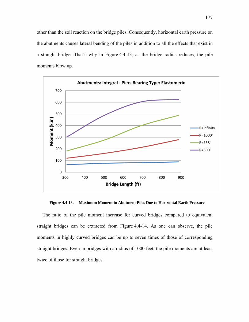
177
other than the soil reaction on the bridge piles. Consequently, horizontal earth pressure on
the abutments causes lateral bending of the piles in addition to all the effects that exist in
a straight bridge. That’s why in Figure 4.4-13, as the bridge radius reduces, the pile
moments blow up.
Figure 4.4-13. Maximum Moment in Abutment Piles Due to Horizontal Earth Pressure
The ratio of the pile moment increase for curved bridges compared to equivalent
straight bridges can be extracted from Figure 4.4-14. As one can observe, the pile
moments in highly curved bridges can be up to seven times of those of corresponding
straight bridges. Even in bridges with a radius of 1000 feet, the pile moments are at least
twice of those for straight bridges.
0
100
200
300
400
500
600
700
300 400 500 600 700 800 900
Mom
ent (k.in)
Bridge Length (ft)
Abutments: Integral ‐ Piers Bearing Type: Elastomeric
R=infinity
R=1000'
R=538'
R=300'

178
Figure 4.4-14. Normalized Moment in Abutment Piles Due to Horizontal Earth Pressure
A8) Centrifugal Force
The results of the study show that the bending moment in the abutment piles due to
centrifugal force is not highly dependent on the radius of curvature or the length of the
bridge. As can be observed in Figure 4.4-15, when the radius of the bridge varies from
300 feet to 1000 feet or the length of the bridge changes between 300 feet and 900 feet,
the pile moments change from 120 to 150 k.in. It means three times of change in radius
or length causes about 25 percent of difference in abutment pile moments. If the
centrifugal force factor was chosen equal to 0.28 for all radii, the pile moments were even
closer to each other.
0.00
1.00
2.00
3.00
4.00
5.00
6.00
7.00
8.00
300 400 500 600 700 800 900
Normalzied
Mom
ent
Bridge Length (ft)
Ratio of Maximum Moments in Abutment Piles(M curved / M straight)
Abutments: Integral ‐ Piers Bearing Type: Elastomeric
R=infinity'
R=1000'
R=538'
R=300'

179
Figure 4.4-15. Maximum Moment in Abutment Piles Due to Centrifugal Force
A9) Weight of Wearing Surface
The response due to the weight of wearing surface has the same style as that of dead
load. As observed in Figure 4.4-16, the pile moments have a decreasing trend as the
length of bridge increases. But the magnitudes of the moments are much smaller. This
can also be interpreted from its weight factor which is equal to two versus the weight of
dead load that is eleven.
0
20
40
60
80
100
120
140
160
180
300 400 500 600 700 800 900
Mom
ent (k.in)
Bridge Length (ft)
Abutments: Integral ‐ Piers Bearing Type: Elastomeric
R=infinity
R=1000'
R=538'
R=300'

180
Figure 4.4-16. Maximum Moment in Abutment Piles Due to Weight of wearing Surface
The ratios of the pile moments for wearing surface weight are shown in Figure 4.4-17.
As the values of the pile moments in this case are not so large, these ratios are not of
great importance from a design point of view.
0
20
40
60
80
100
120
300 400 500 600 700 800 900
Mom
ent (k.in)
Bridge Length (ft)
Abutments: Integral ‐ Piers Bearing Type: Elastomeric
R=infinity
R=1000'
R=538'
R=300'

181
Figure 4.4-17. Normalized Moment in Abutment Piles Due to Weight of Wearing Surface
A10) Braking Force
Braking force shows to be one of the least important load types applied to an integral
bridge. Having a normalized weight factor equal to one implies this minimal effect.
Figure 4.4-18 illustrates the variation of bending moment of the abutment piles versus
bridge length. For all different radii, the braking pile moment increases when the length
of the bridge increases. Another observation is that the braking response for length
greater than 450 feet is different than that of shorter bridges. This is attributed to the way
the loading code defines the braking force. For more evidence one can refer to the
loading section. The other fact is that as the radius of curvature of the bridge increases,
the abutment pile moment due to braking load reduces.
0.00
0.20
0.40
0.60
0.80
1.00
1.20
1.40
300 400 500 600 700 800 900
Normalized
Mom
ent
Bridge Length (ft)
Ratio of Maximum Moments in Abutment Piles(M curved / M straight)
Abutments: Integral ‐ Piers Bearing Type: Elastomeric
R=infinity'
R=1000'
R=538'
R=300'

182
Figure 4.4-18. Maximum Moment in Abutment Piles Due to Braking Force
Figure 4.4-19 depicts the normalized moment of abutment piles for different bridge
lengths and radii. It shows that the pile braking moment of a highly curved bridge is
about four times of that of equivalent straight bridge. But, regarding the fact that the
braking load is of little significance in integral bridges, this increase in the moments is
not so effective in changing the pile design moments.
0
20
40
60
80
100
120
300 400 500 600 700 800 900
Mom
ent (k.in)
Bridge Length (ft)
Abutments: Integral ‐ Piers Bearing Type: Elastomeric
R=infinity
R=1000'
R=538'
R=300'
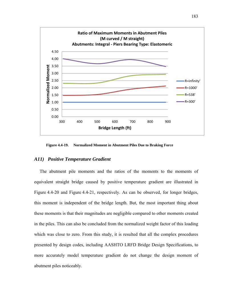
183
Figure 4.4-19. Normalized Moment in Abutment Piles Due to Braking Force
A11) Positive Temperature Gradient
The abutment pile moments and the ratios of the moments to the moments of
equivalent straight bridge caused by positive temperature gradient are illustrated in
Figure 4.4-20 and Figure 4.4-21, respectively. As can be observed, for longer bridges,
this moment is independent of the bridge length. But, the most important thing about
these moments is that their magnitudes are negligible compared to other moments created
in the piles. This can also be concluded from the normalized weight factor of this loading
which was close to zero. From this study, it is resulted that all the complex procedures
presented by design codes, including AASHTO LRFD Bridge Design Specifications, to
more accurately model temperature gradient do not change the design moment of
abutment piles noticeably.
0.00
0.50
1.00
1.50
2.00
2.50
3.00
3.50
4.00
4.50
300 400 500 600 700 800 900
Normalized
Mom
ent
Bridge Length (ft)
Ratio of Maximum Moments in Abutment Piles(M curved / M straight)
Abutments: Integral ‐ Piers Bearing Type: Elastomeric
R=infinity'
R=1000'
R=538'
R=300'

184
Figure 4.4-20. Maximum Moment in Abutment Piles Due to Positive Temperature
Gradient
Figure 4.4-21. Normalized Moment in Abutment Piles Due to Positive Temperature
Gradient
0
5
10
15
20
25
30
300 400 500 600 700 800 900
Mom
ent (k.in)
Bridge Length (ft)
Abutments: Integral ‐ Piers Bearing Type: Elastomeric
R=infinity
R=1000'
R=538'
R=300'
0.00
0.20
0.40
0.60
0.80
1.00
1.20
300 400 500 600 700 800 900
Normalized
Mom
ent
Bridge Length (ft)
Ratio of Maximum Moments in Abutment Piles(M curved / M straight)
Abutments: Integral ‐ Piers Bearing Type: Elastomeric
R=infinity'
R=1000'
R=538'
R=300'

185
A12) Negative Temperature Gradient
The pile moments and normalized moments in the abutments due to negative
temperature gradient are illustrated in Figure 4.4-22 and Figure 4.4-23. Similar to
positive temperature gradient, again the values of bending moments are trifling. The
comment on positive temperature gradient is repeated that complicated modeling for this
type of loading does not distinctly change the design moments.
Figure 4.4-22. Maximum Moment in Abutment Piles Due to Negative Temperature
Gradient
0
1
2
3
4
5
6
7
8
300 400 500 600 700 800 900
Mom
ent (k.in)
Bridge Length (ft)
Abutments: Integral ‐ Piers Bearing Type: Elastomeric
R=infinity
R=1000'
R=538'
R=300'

186
Figure 4.4-23. Normalized Moment in Abutment Piles Due to Negative Temperature
Gradient
A13) Combination of the Loads
The bending moment in the abutment piles are calculated based on the load
combinations of section 4.3.3. As there are several different combinations, study of
responses in all of the combinations may be exhausting. Therefore, the envelope of the
moments in all of those combinations is studied instead. The envelope moments are
plotted for different radii and lengths in Figure 4.4-24. It can be observed that generally
as the radius reduces, the slope of the curves reduces as well. Therefore, in spite of the
larger moments for shorter curved bridges, the moments in curved bridges are finally
smaller than those of the corresponding straight bridge. The other fact is that the envelope
0.00
0.20
0.40
0.60
0.80
1.00
1.20
300 400 500 600 700 800 900
Normalized
Mom
ent
Bridge Length (ft)
Ratio of Maximum Moments in Abutment Piles(M curved / M straight)
Abutments: Integral ‐ Piers Bearing Type: Elastomeric
R=infinity'
R=1000'
R=538'
R=300'

187
pile moments of bridge with small radius of curvature, R<600 feet, is almost independent
of the bridge length. This is a significant result that can be concluded from this graph.
Figure 4.4-24. Maximum Moment in Abutment Piles in Load Combinations Envelope
Similar to what was done for each load case; the normalized moments are plotted
versus bridge length for different radii of curvature in Figure 4.4-25. In this graph, it is
shown that in bridges of length less than 500 feet, pile design moment in curved bridges
are at most 20 percent larger than those of straight bridges. But as the length of the bridge
increases, the moments reduce in a manner that in bridges of length equal to about 900
feet and radii equal to 300, 538 and 1000 feet, the pile moments are 0.48, 0.54 and 0.81
times of those of equivalent straight bridge, respectively.
0
1000
2000
3000
4000
5000
6000
7000
300 400 500 600 700 800 900
Mom
ent (k.in)
Bridge Length (ft)
Abutments: Integral ‐ Piers Bearing Type: Elastomeric
R=infinity
R=1000'
R=538'
R=300'

188
Figure 4.4-25. Normalized Moment in Abutment Piles in Load Combinations Envelope
B) Shear Force of Abutment Piles
A study similar to what is done for abutment piles bending moment is carried out on
the shear forces of the piles. The results show that the design shear force of piles which is
the envelope of the shear in different load combinations is increasing in straight bridges
as the length of the bridge increases. But in curved bridges, such a general conclusion
cannot be made. The response depends on the radius of curvature of the bridge. It is
observed that for bridges with large radius, the behavior is similar to that of straight
bridges. In the bridges of high curvature, the slope of shear curves is much smaller than
that of bridges with large radius so that the shear forces can even be decreasing versus
length. In long bridges with small radius, the design shear can be as small as 40 percent
of that of equivalent straight bridges.
0.00
0.20
0.40
0.60
0.80
1.00
1.20
1.40
300 400 500 600 700 800 900
Normalized
Mom
ent
Bridge Length (ft)
Ratio of Maximum Moments in Abutment Piles(M curved / M straight)
Abutments: Integral ‐ Piers Bearing Type: Elastomeric
R=infinity'
R=1000'
R=538'
R=300'

189
For brevity of the main text, the complete discussions and graphs of shear forces in
abutment piles are presented in Appendix A.
4.4.2 Bridge Movement
Bridge movement is a major concern in design of integral bridges. When the
superstructure of a bridge is integrally connected to the abutments, all effects that can
cause a displacement or rotation at the ends of the bridge create internal forces both in
abutment and in superstructure. The most important source of displacing the end of a
bridge is temperature change. Expansion and contraction are the most known causes of
change of bridge length. The other significant reason for bridge movement is the
shrinkage of concrete deck. In fully concrete superstructures, shortening of the bridge
length can also be caused by creep of concrete. However, in composite steel bridges
creep cannot have such a role in moving the ends of the bridge. When there is a
movement in the bridge ends, all the bridge elements including abutment wall, abutment
piles, steel girders and deck should tolerate the induced forced. The pavements should
also accommodate the movement so that there is not uncontrolled cracks or bumps in the
road.
In order to determine the displacements of bridge ends, all the engaged factors should
be studied. These include:
- the factors dependent on the location and type of the bridge: maximum and
minimum temperatures that the bridge experiences over its life span, the
temperature gradient in the bridge elements, construction temperature of the bridge
190
- the factors dependent on material properties: coefficients of thermal expansion of
steel and concrete, creep and shrinkage properties of concrete
- the factors affecting the bridge movement based on the structural characteristics of
the bridge
The first set of problems which are mainly climatic problems have been studied by
several researchers. As these problems depend on many parameters including shade
temperature, solar radiation and wind speed, the success in this area has been limited. But
reasonable data are available in references including “Climatic Atlas of the United
States” (Visher, 1954) and “Climatography of the United States” (United States,
Environmental Data Service, & National Climatic Center, 1900s). In the present study,
an increase of +60 °F and a decrease of -100 °F are taken which are based on AASHTO
LRFD contour maps for a typical location in the US. But site specific temperatures
should be used for each bridge which can be obtained from climatological resources or
design codes.
The second set of problems which is determination of the material properties is also
studied by several researchers, including the investigations of Tadros et al. on the creep
and shrinkage properties of concrete (Al-Omaishi, Tadros, & Seguirant, 2009; Huo, Al-
Omaishi, & Tadros, 2001; Tadros et al., 2003).
But the third problem which is analysis of bridges for movements due to assumed
temperature changes and assumed material properties needs much more attention. What
is generally known in bridge engineering is that the bridge movement if the summation of
the movements due to temperature, shrinkage and creep:

191
∆ ∆ ∆ ∆ Eq. 4.16
The thermal displacement is equal to the thermal strain times the initial length:
∆ Eq. 4.17
In which thermal strain is the product of temperature change ∆ and the coefficient of
thermal expansion . The shrinkage and creep displacements are also calculated in the
same way:
∆ Eq. 4.18
and
∆ Eq. 4.19
To calculate the shrinkage and creep strains there are some available methods, one of
them the equations presented by AASHTO LRFD Bridge Design Specifications
(American Association of State Highway and Transportation Officials, 2010). But
regarding the usage of these equations, some questions may come to the mind of a bridge
engineer:
- Are these equations able to predict the bridge movement with enough precision?
- Aren’t there any other factors affecting the bridge displacement at pavement level?
- What should be done to find the displacements of a curved bridge?
In this section, using the finite element models of the studied composite steel curved
bridges, it is tried to answer the above questions. First, a discussion is presented to clarify
the involved factors and the difference of bridge shortening and bridge end displacement.
Then, based on the results of finite element analyses, two factors are introduced to more
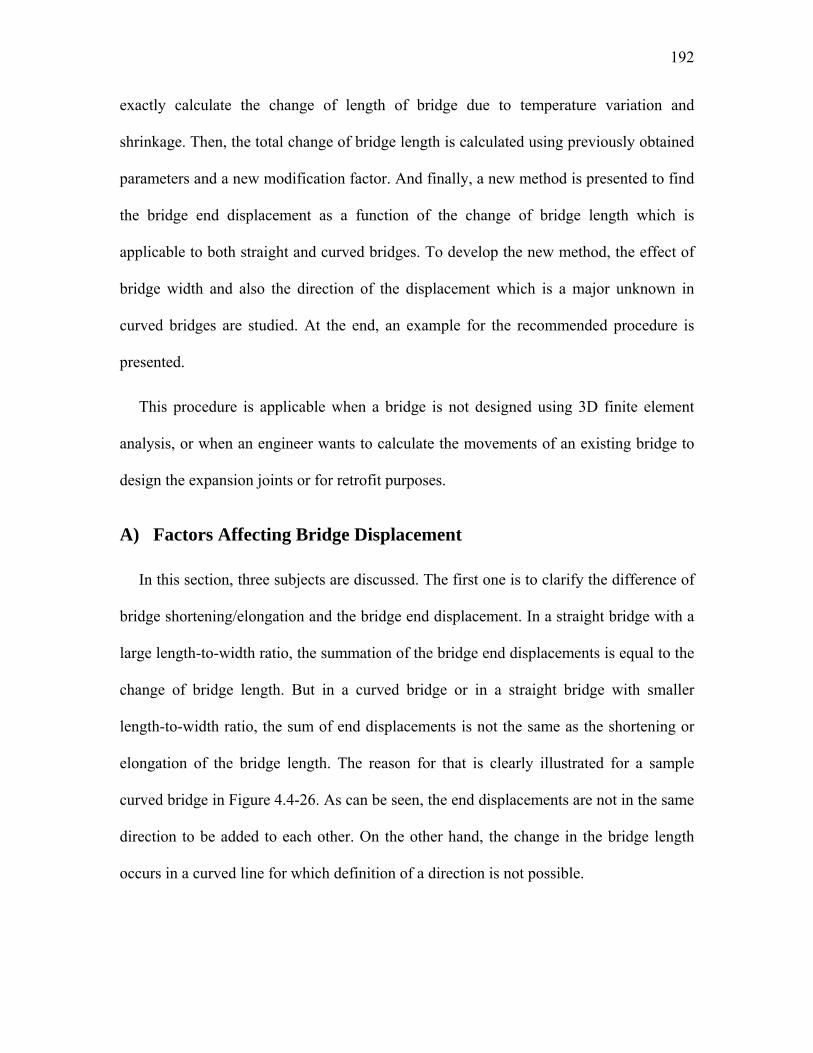
192
exactly calculate the change of length of bridge due to temperature variation and
shrinkage. Then, the total change of bridge length is calculated using previously obtained
parameters and a new modification factor. And finally, a new method is presented to find
the bridge end displacement as a function of the change of bridge length which is
applicable to both straight and curved bridges. To develop the new method, the effect of
bridge width and also the direction of the displacement which is a major unknown in
curved bridges are studied. At the end, an example for the recommended procedure is
presented.
This procedure is applicable when a bridge is not designed using 3D finite element
analysis, or when an engineer wants to calculate the movements of an existing bridge to
design the expansion joints or for retrofit purposes.
A) Factors Affecting Bridge Displacement
In this section, three subjects are discussed. The first one is to clarify the difference of
bridge shortening/elongation and the bridge end displacement. In a straight bridge with a
large length-to-width ratio, the summation of the bridge end displacements is equal to the
change of bridge length. But in a curved bridge or in a straight bridge with smaller
length-to-width ratio, the sum of end displacements is not the same as the shortening or
elongation of the bridge length. The reason for that is clearly illustrated for a sample
curved bridge in Figure 4.4-26. As can be seen, the end displacements are not in the same
direction to be added to each other. On the other hand, the change in the bridge length
occurs in a curved line for which definition of a direction is not possible.

193
Figure 4.4-26. Directions of End Displacements in A Curved Bridge
The second problem is to investigate the reasons for “movement” of bridge ends.
Among the applied loads and load effects to a bridge, some of them like temperature
variation change the bridge length. It is obvious that when the length of a bridge changes,
at least one of the bridge ends moves. But this kind of movement is not the only source
for bridge end displacement. The bridge ends can displace due to rotation of the bridge
ends without noticeable change in bridge length. This rotation is more understandable as
a source of movement when the load do not change bridge length, like gravity loads.
Figure 4.4-27 shows a picture of bridge end movement due to translation and rotation.
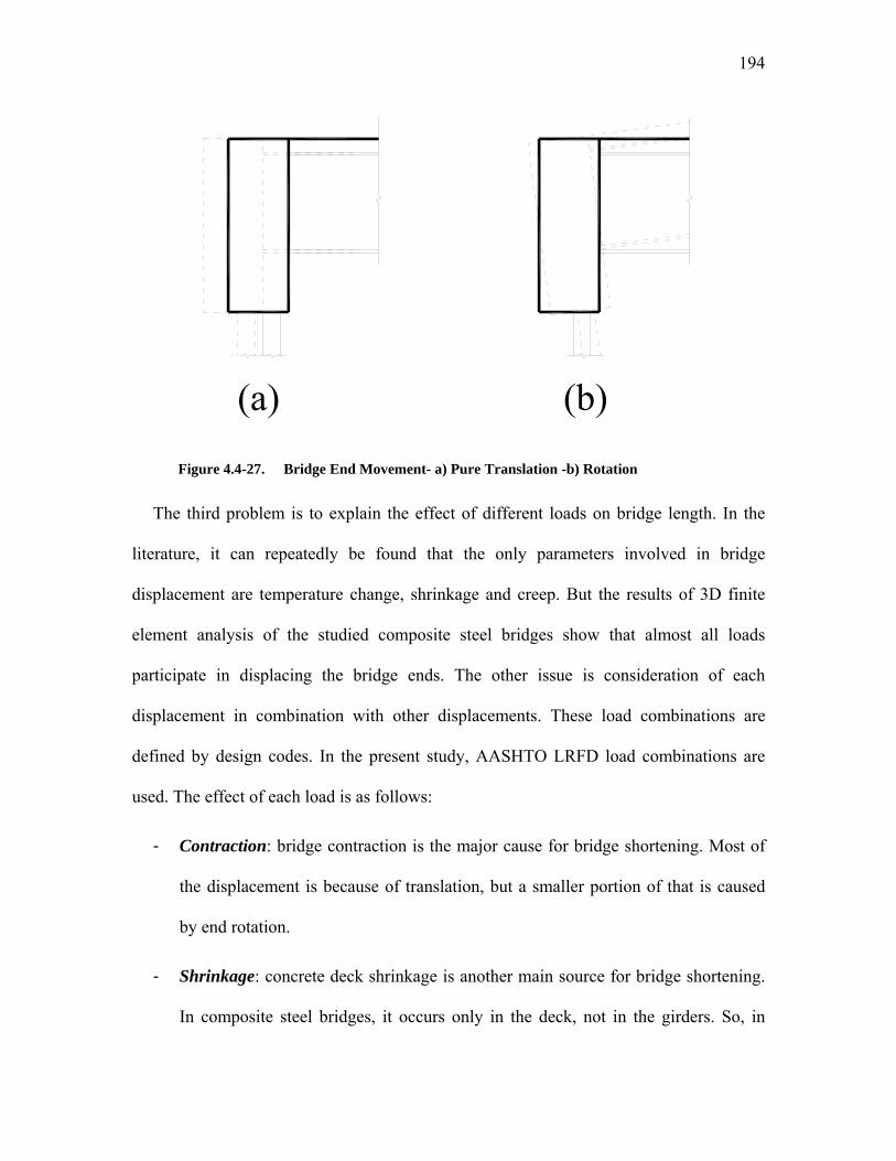
194
Figure 4.4-27. Bridge End Movement- a) Pure Translation -b) Rotation
The third problem is to explain the effect of different loads on bridge length. In the
literature, it can repeatedly be found that the only parameters involved in bridge
displacement are temperature change, shrinkage and creep. But the results of 3D finite
element analysis of the studied composite steel bridges show that almost all loads
participate in displacing the bridge ends. The other issue is consideration of each
displacement in combination with other displacements. These load combinations are
defined by design codes. In the present study, AASHTO LRFD load combinations are
used. The effect of each load is as follows:
- Contraction: bridge contraction is the major cause for bridge shortening. Most of
the displacement is because of translation, but a smaller portion of that is caused
by end rotation.
- Shrinkage: concrete deck shrinkage is another main source for bridge shortening.
In composite steel bridges, it occurs only in the deck, not in the girders. So, in
(a) (b)

195
addition to reducing the length of the bridge, it causes rotation of the ends more
profoundly compared to bridge contraction.
- Creep: the effect of concrete creep is ignorable in composite steel bridges.
However in prestressed concrete bridges, it is an important reason for bridge
shortening.
- Expansion: bridge expansion is another significant source of displacing the bridge
ends. In section 4.4.1A2), two reasons were presented for smaller abutment pile
moments due to expansion compared to contraction. For exact same reasons, the
displacements due to expansion are smaller than those of contraction. In addition,
contraction, shrinkage and creep create displacements that are in the same
direction (or at least approximately in the same direction). But expansion
movement is almost in the opposite direction. In the conducted finite element
analyses, expansion load combinations do not create the maximum end
displacements. For these reasons, the main focus of the present study is to
calculate the bridge movements in contraction load combinations.
- Gravity Loads including dead load, weight of wearing surface and live load: all
gravity loads cause bridge end displacement. As gravity loads do not change the
bridge length, this displacement is mainly due to rotation of the bridge ends.
- Lateral loads: these loads such as centrifugal load and wind load are analyzed in
the finite element models. The results demonstrate that the movements due to this
type of loads are not of great importance. Although all of these displacements are
taken into account.

196
- Earth pressure: finite element analyses of the studied bridges show that earth
pressure has a minimal effect on end displacement of straight bridges. But in the
case of curved bridges, its effect become more visible which is considered in the
models.
- Braking force: the results show that live load braking force has a minimal effect
on bridge movement.
- Temperature gradient: all model either straight or curved show that the
displacements due to temperature gradient in superstructure in approximately zero.
So, if a bridge designer ignores the complicated modeling of temperature gradient,
no noticeable displacement is missed.
B) Bridge Shortening Due to Contraction
To calculate the reduction of the bridge length due to a uniform temperature decrease
of -100 °F, the equivalent coefficient of thermal expansion (in this case contraction)
should be evaluated. This coefficient is calculated as follows:
Eq. 4.20
in which the values of modulus of elasticity, E, cross sectional area, A, and coefficient of
thermal expansion, , for concrete deck and steel girder should be plugged in. Then, the
change of bridge length can be calculated using the following equation:
∆ . ∆ . Eq. 4.21
where ∆ is equal to -100 °F and is the initial length of the bridge (or
√ where and are the undeformed bridge length and width to account for the

197
effect of bridge width). Based on the location of point of zero movement, this value may
be multiplied by a fraction like ½. For curved bridges, two different lengths for inner and
outer arc of the bridge are considered. Comparison of the bridge length reductions
resulted from 3D finite element analyses and hand calculations based on the above
equations shows differences that are mainly due to bending moments in the cross section.
The ratio of the lengths resulted from finite element analyses and the lengths based on
hand calculations are defined as a modification factor that is plotted versus the
radius of curvature in Figure 4.4-28. For simplicity, in hand calculations, the actual
distance to the point of zero movement, which is an oblique line in straight bridges and
an unknown curve in curved bridges, is ignored and the modification factors are found
based on the length of the bridge edges.
Figure 4.4-28. Modification Factor for Bridge Shortening Due to Contraction
0.9
0.95
1
1.05
1.1
1.15
100 1000 10000
Mod
ification
Factor, gTU
c
Radius (ft)
Outer Arc
Inner Arc

198
C) Bridge Shortening Due to Shrinkage
To calculate the change in bridge length because of shrinkage of concrete, the
equivalent shrinkage strain of superstructure due to shrinkage of different components
should be determined as follows:
, , , , Eq. 4.22
The shrinkage strain for each component should be calculated based of the
recommendations of 4.3.2J). It should be noted that , for steel girders is equal to
zero. Then the change in bridge length is calculated as follows:
∆ , Eq. 4.23
in which is the bridge length in straight bridges and the inner and outer arc length in
curved bridges (or or a fraction of this value). Comparison of
the results of these calculation and the bridge lengths resulted from 3D finite element
analyses shows that the hand calculations need a modification factor to account for all of
the other participating factors that are not seen in these simplified calculations. This
factor, named , is plotted versus radius of curvature for the modeled bridges.

199
Figure 4.4-29. Modification Factor for Bridge Shortening Due to Shrinkage
D) Total Bridge Shortening
The total bridge shortening can be found as the shortening due to contraction and
shrinkage are available from previous sections. The changes in lengths of the bridges are
obtained based on AASHTO LRFD Service I load combinations. In these load
combinations, temperature and shrinkage can have a load factor of 1.2 to yield the
maximum response. So, the values of bridge length reduction obtained from finite
element analyses are compared to the values of length reduction found from 1.2 times of
contraction and shrinkage calculation. The values of bridge length reduction of 3D
models are obtained from drawing of the deformed shapes of the bridges in AutoCAD.
Finding bridge length using these two different methods again demonstrates that hand
calculations miss the effect of some other parameters that exist in a real bridge. These
parameters include other loads such as gravity and lateral loads and also earth pressure.
1.1
1.15
1.2
1.25
1.3
1.35
1.4
1.45
100 1000 10000
Mod
ification
Factor, gSh
Radius (ft)
Outer Arc
Inner Arc

200
To account for these parameters another modification factor is defined which is plotted
versus radius in Figure 4.4-30.
Figure 4.4-30. Modification Factor for Bridge Shortening Applied to Total Shortening
As can be observed, the summation of contraction and shrinkage shortenings should
be increased from 5 to 8 percent to make up for the effect of other loads. So, the total
shortening of a bridge, either straight or curved, is computed using the following
equation:
∆ 1.2 ∆ ∆ Eq. 4.24
If the modification factor given by Figure 4.4-30 is assumed to be equal to 1.08 for all
bridges, then the Eq. 4.24 is simplified to:
∆ 1.3 ∆ ∆ Eq. 4.25
0.9
0.95
1
1.05
1.1
1.15
1.2
100 1000 10000
Mod
ification
Factor, g
Radius (ft)
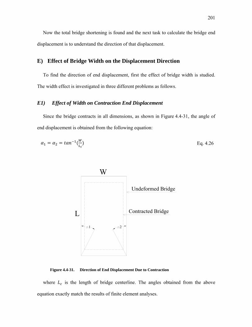
201
Now the total bridge shortening is found and the next task to calculate the bridge end
displacement is to understand the direction of that displacement.
E) Effect of Bridge Width on the Displacement Direction
To find the direction of end displacement, first the effect of bridge width is studied.
The width effect is investigated in three different problems as follows.
E1) Effect of Width on Contraction End Displacement
Since the bridge contracts in all dimensions, as shown in Figure 4.4-31, the angle of
end displacement is obtained from the following equation:
Eq. 4.26
Figure 4.4-31. Direction of End Displacement Due to Contraction
where is the length of bridge centerline. The angles obtained from the above
equation exactly match the results of finite element analyses.
L
W
21
Undeformed Bridge
Contracted Bridge

202
E2) Effect of width on Shrinkage End Displacement
The direction of shrinkage end displacement is more complicated. Since the girders
are continuous in the longitudinal direction of the bridge and discrete in the transverse
direction, the following equation can be imagined for the direction of the displacement:
Eq. 4.27
These angles are also compared to the finite element results which show reasonable
and practical precision.
E3) Effect of width on Total End Displacement
The effect of bridge width on the total bridge displacement is much more complicated
than the previous cases and derivation of a closed for solution for that is not easily
possible. Therefore, a finite element solution is employed. Based on the results of the
finite element analyses, the data presented in Table 4.4-2 are gathered that are used to
find the effect of bridge width on the total displacement of bridges.
L (ft) W/L (deg.) /90° (deg.) /90°
308 0.197 105 1.17 75 0.83
501 0.121 100 1.11 80 0.89
694 0.087 98 1.09 82 0.91
887 0.068 96 1.07 84 0.93
Infinity 0.000 90 1.00 90 1.00
Table 4.4-2. Direction of Total Displacement (Results of FE Analyses) (W=60’-8”)

203
The angles and are shown in Figure 4.4-32.
Figure 4.4-32. Angles and in Total Displacement
If the values of /90° and /90° are plotted versus W/L, as shown in
Figure 4.4-33, it is observed that these values can be estimated by two lines with a good
correlation. The following two equations are presented for these two lines:
1 0.84 Eq. 4.28
1 0.84 Eq. 4.29
L
Undeformed Bridge
Deformed Bridge
in
out

204
Figure 4.4-33. Values / ° versus W/Lc
The values of the above two equations are deviation of the direction of displacements
from 90 degrees because of the width of the bridge. These equations can be considered as
the effect of width on the direction of total displacement. The ratio of / should be
limited to 0.33 for these equations.
F) Direction of Displacement
In this section, it is tried to find the direction of the bridge end displacements based on
the results of the finite element analyses of the modeled bridges and also the findings the
previous section on the effect of bridge width.
In the previous section the factors and were found that represent the effect of
bridge width on the direction of end movements. If the angles of displacement are
divided by these factors, the effect of bridge width is excluded from displacement
direction. So, the obtained angles can be more easily handled as the effect of curvature on
displacement direction. Based on this finding, the direction of movements for the studied
y = 0.8399x + 1.0072R² = 0.9884
y = ‐0.8399x + 0.9928R² = 0.9884
0.00
0.20
0.40
0.60
0.80
1.00
1.20
1.40
0 0.05 0.1 0.15 0.2 0.25
a/ 90
°
W/L
Inner angle
Outer Angle
Linear (Inner angle)
Linear (Outer Angle)

205
bridges are derived from finite element models and by dividing those angles by the
factors and , it is tried to find a relationship for the modified directions.
Table 4.4-3 shows the angles of displacement direction for different bridges and the
modified directions to eliminate to effect of width.
206
L R L/R , ,
308 300 1.03 91 78.0 67 80.0
501 300 1.67 77 69.0 60 68.0
694 300 2.31 68 62.4 57 63.0
887 300 2.96 68 64.0 58 62.0
308 538 0.572 102 87.0 73 87.0
501 538 0.931 86 77.5 70 78.8
694 538 1.29 82 75.0 68 75.0
887 538 1.649 76 71.0 65 69.6
308 1000 0.308 104 89.5 74 89.0
501 1000 0.501 94 84.7 76 85.5
694 1000 0.694 88 80.7 75 82.3
887 1000 0.887 85 79.4 75 80.4
308 Infinity 0 105 90.0 75 90.0
501 Infinity 0 100 90.0 80 90.0
694 Infinity 0 98 90.0 82 90.0
887 Infinity 0 96 90.0 84 90.0
Table 4.4-3. Angles and Modified Angles of Total Displacement Direction
The values of modifies angles are plotted versus the ratio L/R in Figure 4.4-34.

207
Figure 4.4-34. Modified Displacement Directions versus L/R
As observed in Figure 4.4-34, the modified inner and outer angles surprisingly
coincide. If a line is fitted to the data series of the modified angles, a unique equation is
obtained which is displayed in Eq. 4.30.
90° 11 Eq. 4.30
Then the actual values of inner and outer angles can be calculated using the following
equations:
. Eq. 4.31
. Eq. 4.32
In this way, the direction of end displacement of a curved bridge can be determined.
G) Bridge End Displacement
In the previous sections, the magnitude of the total shortening of bridges which is a
function of contraction and shrinkage shortening and some modification factors and also
y = ‐11.04x + 90.248R² = 0.9576
y = ‐10.586x + 89.684R² = 0.9397
0
10
20
30
40
50
60
70
80
90
100
0 1 2 3 4
Mod
ified
Angles
L/R
Modified Outer Angle
Modified Inner Angle
Linear (Modified Outer Angle)
Linear (Modified Inner Angle)

208
the direction of the end displacements of the corners of a curved bridge were found. In
this section, the goal is to calculate the total end displacements of a bridge, based on the
previous findings. For that purpose, one of the arcs of the bridge, either inner or outer, is
considered. The problem needs a geometrical solution to find a new arc which has a
specific length and its end lies on a specific line. The specific length is the length of the
deformed bridge and the specific line is the direction of the end displacement, which both
of them are known. The geometry of the problem is shown in Figure 4.4-35. In this
picture, the undeformed configuration is known which consists of the length L, the radius
R and the center of curvature O. So, the coordinates of all of the points on the curve are
known. Desired is to locate the deformed curve which means finding O’ and R’ knowing
the new length L’ and the line AA” as the geometrical location for A’.
Figure 4.4-35. Deformed Bridge General Configuration
After trying to solve this problem, it was found out that this problem does not have a
unique solution. So, one more constraint should be added to the problem. Drawing the
O
O'A
A'
A"L/2L'/2
x
y
B'
OB=RO'B'=R'
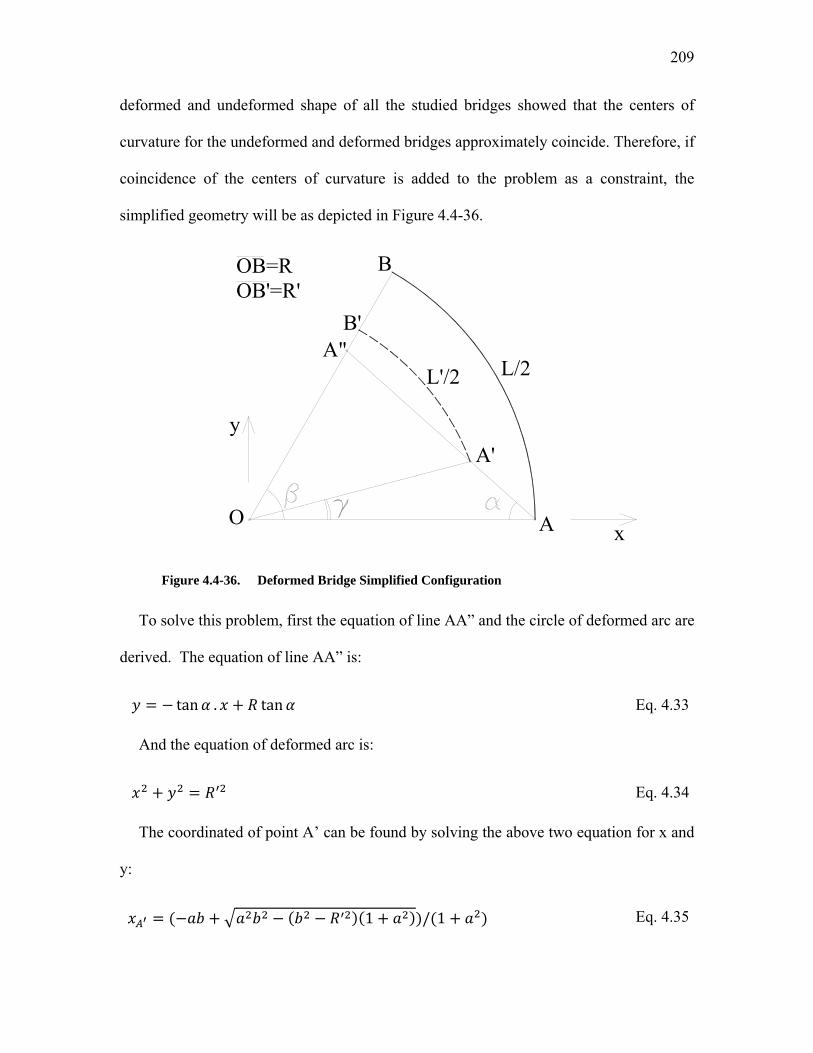
209
deformed and undeformed shape of all the studied bridges showed that the centers of
curvature for the undeformed and deformed bridges approximately coincide. Therefore, if
coincidence of the centers of curvature is added to the problem as a constraint, the
simplified geometry will be as depicted in Figure 4.4-36.
Figure 4.4-36. Deformed Bridge Simplified Configuration
To solve this problem, first the equation of line AA” and the circle of deformed arc are
derived. The equation of line AA” is:
tan . tan Eq. 4.33
And the equation of deformed arc is:
Eq. 4.34
The coordinated of point A’ can be found by solving the above two equation for x and
y:
1 / 1 Eq. 4.35
O A
A'
A"L/2L'/2
x
y
B
B'
OB=ROB'=R'

210
Eq. 4.36
Where
tan Eq. 4.37
tan Eq. 4.38
So the slope of line OA’ will be:
tan Eq. 4.39
The length of the deformed arc is equal to:
2 Eq. 4.40
In which
Eq. 4.41
The above equations can be solved numerically to find R’. This can be done easily in
Excel, MathCAD, MATLAB or any other program capable of solving equations. The
Excel is maybe the easiest one. Note that in these equations, is the total length, not half
of it.
Using the presented method, the end displacements of a curved composite steel bridge
are found which is of great importance to design such a bridge. This method is also
helpful to have a sense of magnitude and direction of displacements to design the bridge-
to-pavement connection devices like the expansion joints.

211
H) Step by Step Procedure
Based on the investigations of the present study, the following steps are recommended
to calculate the maximum displacements of a curved or straight bridge:
Step 1- Determine the point of zero movement and therefore the length of the bridge
that participates in end displacement. For symmetric bridges, it can be assumed to be
equal to half of the length of bridge. Otherwise, other methods found in the literature can
be employed. To account for the effect of width, can be replaced by √ or a
similar function of bridge length and width.
Step 2- Determine the effective coefficient of thermal expansion using Eq. 4.20.
Step 3- Calculate the bridge shortening due to contraction using Eq. 4.21.
Step 4- Find the modification factor for bridge shortening due to contraction using
Figure 4.4-28.
Step 5- Determine the equivalent shrinkage strain using Eq. 4.22 and
recommendations of 4.3.2J).
Step 6- Calculate the bridge shortening due to shrinkage using Eq. 4.23.
Step 7- Find the modification factor for bridge shortening due to shrinkage using
Figure 4.4-29.
Step 8- Find the modification factor for total bridge shortening using Figure 4.4-30.
Step 9- Calculate the total bridge shortening using Eq. 4.24.
Step 10- Calculated the bridge width effect factor using Eq. 4.28 and Eq. 4.29.

212
Step 11- Find the direction of the bridge corners displacements solving Eq. 4.30
through Eq. 4.32.
Step 12- Knowing the total bridge shortening found in step 9 and the directions found
in step 11, solve equations Eq. 4.35 through Eq. 4.41 to find the new location of bridge
corners.
Using this method, the x and y components of bridge end displacements are found.
I) Example
In this section, the x and y components of the end displacement of the inner corner of
a curved composite steel bridge of length, width and radius of curvature respectively
equal to 887, 60.667 and 538 feet are calculated.
Assumptions:
3644
864
6.0 10 /
29000
99.35
6.5 10 /
1- It is assumed that point of zero movement is located in the middle of the bridge.
887538 538
60.6672 12 10043.88

213
2 5021.94
2- Equivalent coefficient of thermal expansion:
. . ..
6.24 10 /
3- Contraction shortening is equal to:
∆ . ∆ . 6.24 100 5021.94 3.134
4- From Figure 4.4-28:
0.97
5- Equivalent shrinkage strain:
, 0
, 538 10 (From section 4.3.2J))
, , , , 538 10
.304.5 10
6- Shrinkage shortening:
∆ , /2 304.5 10 5021.94 1.529
7- From Figure 4.4-29:
1.185
8- From Figure 4.4-30:
1.07

214
9- Total shortening is:
∆ 1.2 ∆ ∆ 1.2 1.07 0.97 3.134 1.185
1.529 6.23
10- Effect of width on displacement direction:
1 0.84 1 0.84 . 1.057
11- Direction of displacement:
90° 11 90 11 71.7°
. 1.057 71.7 75.8°
12- Solving equations Eq. 4.35 through Eq. 4.41:
6090.70 .
5.15 .
So:
∆ 6090.70 538 . 12 1.30 .
∆ 5.16 0 5.16 .
∆ and ∆ are the components of displacement of the inner corner of the bridge.
4.4.3 Pile Orientation
There are two different opinions on the orientation of abutment piles among the
researchers of this field. A first approach to pile orientation in integral bridges, asks for
the weak axis bending for the piles. The supporters of such an attitude have the following
reasoning for their opinion: As the bridge tends to move longitudinally and as this

215
movement depends on the length of the bridge which can be hundreds of feet, in order to
facilitate the bridge end displacement, the stiffness of the abutments should be
minimized. One of the most effective methods to reduce the stiffness of the abutments is
to align the piles of the abutment such that the bending moment due to longitudinal
movement occurs about the weak axis of the piles. This philosophy has led several
departments of transportation to require a weak-axis bending orientation for the abutment
piles. But, in contrast to this interpretation, another approach regards the problem mainly
as a classic bending problem in which larger section modulus of an element results in
smaller normal stresses. Founded on the latter reasoning, some other departments of
transportation necessitate strong axis orientation for the abutment piles. Figure 4.4-37
illustrates the weak- and strong-axis orientations for the abutment piles.
Figure 4.4-37. Critical Load Combination Type
It is observed that there is disagreement on the pile orientation among bridge
researchers. The first approach has more supporters. In a report submitted to Virginia
Department of Transportation, it is clearly written that: “Steel H-piles are often oriented
Pile
Concrete Wall
Span
A A
Section A-A
Bridge Longitudinal Axis
Section A-A
Weak-Axis Strong-Axis

216
for weak-axis bending to better accommodate bridge displacements. For a given
deflection, weak-axis bending generates less stress in the piles than does strong-axis
bending.” Or “In order to build longer integral bridges, pile stresses should be kept low.
In addition to weak-axis bending orientation of piles, additional provisions can be made”
(Arsoy et al., 1999). It seems that the writers have assumed the same fixity depth and the
same section modulus for the piles oriented in weak and strong axes in order to so easily
conclude that weak orientation develops less stresses. If two elements have the same
length and different moment of inertia, due to equal lateral displacement, the bending
moment in that one which has smaller moment of inertia will be smaller. This relation
can be clearly seen in Eq. 4.42.
∆ Eq. 4.42
But such two piles embedded in soil do not have the same points of fixity. As the
moment of inertia increases, the fixity point will be deeper. On the other hand, the section
modulus of the weak axis is smaller than that of the strong axis. And the stress is directly
related to section modulus, not the moment of inertia. So even if it is definitely known
that the bending moment about the weak axis is smaller than the strong axis, it cannot be
concluded that the stress level in the pile is lower.
According to the above explanations, it is clear that pile orientation is a more
complicated problem than what apparently assumed by some designers. More complexity
comes to existence when the bridge has some sort of irregularity such as horizontal
curvature.
As stated earlier, this problem depends on some factors including bridge configuration
and soil properties. The other factor is the loading that is dictated by the design code. To

217
be able to have a closer approach to this problem, first, the studies bridges are analyzed
with usual weak axis orientation for the piles, assuming a moderate stiffness for the soil
as explained in Section 4.3.4. Then, all bridges are analyzed with the piles aligned so that
their strong axis is parallel to abutments. After studying the resulted internal forces, a
method for orienting the abutment piles of a general curved bridge in the optimized
direction is derived. In the proposed method, the goal is to minimize the stresses of the
piles. It is also explained that why minimizing the stresses is in agreement with LRFD
approach for design of piles, because one may think of it as an allowable stress design
methodology.
A) Analysis of Modeled Bridges with Weak and Strong Orientation for
Abutment Piles
In this section, first, to have a better understanding of the effect of pile orientation on
the developed stresses in the bridge elements and particularly in the abutment piles, all
the modeled bridges are analyzed in both usual cases for pile orientation. Since the
baseline bridge had a weak axis parallel to abutments, all the original finite element
models have weak axis orientation for the piles. So, the results presented in section 4.4.1
are for weak axis orientation. The piles of all models are rotated 90 degrees so that the H-
Piles strong axes become parallel to the abutments. These new models are analyzed and
the maximum stresses in the piles of all bridges are calculated using the following
equation:
Eq. 4.43

218
In the above equation, is the axial load of the pile, is the cross sectional area of the
pile, , , and are the bending moment and section modulus of the pile
about the weak axis and strong axis, respectively. The ratios of the maximum stresses of
the piles in the original weak axis oriented models to those of the new models with strong
axis orientation are shown in Table 4.4-4.

219
L (ft)
R (ft) 308 501 694 887
300 0.84 0.87 0.76 0.80
538 0.86 0.90 1.23 1.20
1000 0.96 0.96 1.40 1.60
Infinity 1.65 1.48 1.60 1.71
Table 4.4-4. Ratios of Abutment Pile Stresses (Weak Axis Orientation to Strong Axis
Orientation)
As can be observed from the above table, in some cases the weak-axis bending leads
to lower stresses and in some other cases strong-axis orientation yields smaller stress
values. So, a general conclusion cannot be made at this stage. The other important
observation is that in straight bridges, the ratio is greater than unity, no matter what is the
length of the bridge. It means lower stresses for strong-axis orientation. This can be
theoretically proven regarding the fact that bridge end displacement is almost
independent of the substructure stiffness. So, the parameter ∆ in Eq. 4.42 is equal for all
pile orientations. Besides, normal stress due to bending is equal to:
Eq. 4.44
in which is half of the depth of a symmetric section. Substituting from Eq. 4.42 into
Eq. 4.44 yields:
∆ Eq. 4.45
As the depth and width of HP sections are approximately equal, the parameter c is the
same for weak and strong axes bending ( ). The length L is the distance
220
from top of the pile to the point of fixity which is calculated using the following
equations for different soil properties:
1.4 for constant Eq. 4.46
And
1.8 for linearly increasing Eq. 4.47
Therefore, assuming the same soil properties, is larger for strong axis orientation.
Therefore, based on Eq. 4.45, as ∆ is the same for both orientations, will be smaller
for strong axis bending. In HP sections strong axis moment of inertia is about three times
of that of weak axis. So, is about 30 percent larger for the strong axis and so the stress
is about 25 percent lower. This difference is only due to horizontal displacement. Other
factors such as pile rotation due to earth pressure or any other participating factor can
also affect the stresses. That’s why larger differences are read from Table 4.4-4 for
straight bridges.
To further investigate the effect of pile orientation, the condition under which a load
combination produces the maximum stress in the abutment piles is studied. To have such
a discussion, first the individual loads are considered. Gravity loads including dead load,
live load and weight of future wearing surface are the first set of loads that create
noticeable stress levels in the abutment piles. In a bridge of simple geometry like a
straight bridge, these loads apply an axial load and a negative moment to the abutment
piles. Temperature and shrinkage are the second set of loads that cause considerable
amount of stress in the piles. In this set, expansion applies negative moment to the
abutments, while contraction and shrinkage apply positive moment to the abutments. If

221
other loads such as centrifugal force, braking force, earth pressure, wind load and
temperature gradients are ignored, the positive and negative moments of the piles can be
written as follows:
. . . ∆ Eq. 4.48
And
& . . . ∆ . Eq. 4.49
In which is the span length, is the total length of the bridge, ∆ is the uniform
temperature change and , and are constants. Plugging in the values of temperature
changes, the above two equations can be rewritten as:
. 60 . Eq. 4.50
And
& . 100 . . Eq. 4.51
The last two equations show that for short bridges the negative moment is greater than
the positive moment but as the length of the bridge increases, the positive moments due
to contraction becomes dominant. It should be noted that the axial force stresses are
added to the bending stresses, independent of the bending moment direction. Therefore,
the load combinations can be divided into two types:
- The load combinations that include bridge expansion (denoted as EXP.).
- The load combinations that include bridge contraction (denoted as CONT.).

222
With this background on the developed stresses in the piles, using the results of finite
element analyses, the governing load combination category for each model is determined.
The results for weak-axis bending pile orientation are shown in Table 4.4-5.
L (ft)
R (ft) 308 501 694 887
300 EXP. EXP. CONT. CONT.
538 EXP. CONT. CONT. CONT.
1000 EXP. CONT. CONT. CONT.
Infinity EXP. CONT. CONT. CONT.
Table 4.4-5. Critical Load Combination Category for Abutment Pile Stresses
Table 4.4-5 shows that bridges of short length have an expansion-based critical load
combination and in other bridges the load combinations that include contraction dominate
the stresses. In bridges of very small radius of curvature, the criticality of expansion load
combinations extends more into longer bridges, but as the length increases, contraction
becomes governing again. On this basis, a graph can be plotted for determining the
governing load combination in the studied bridges that is shown in Figure 4.4-38.
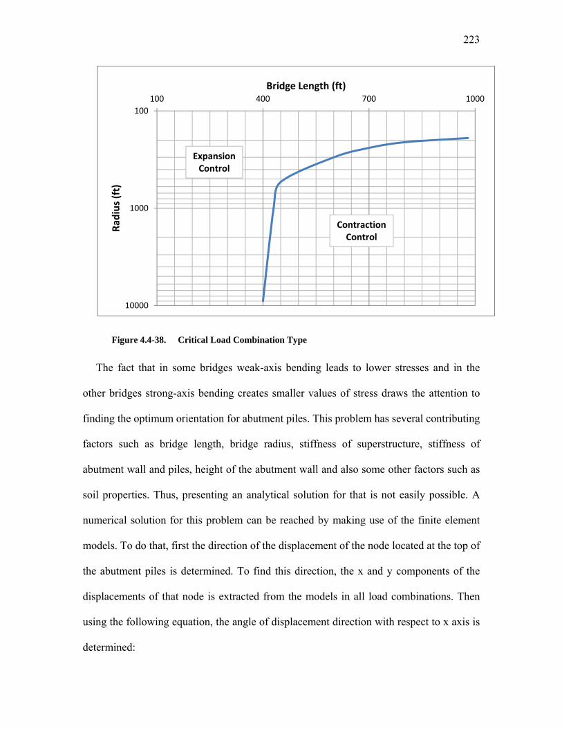
223
Figure 4.4-38. Critical Load Combination Type
The fact that in some bridges weak-axis bending leads to lower stresses and in the
other bridges strong-axis bending creates smaller values of stress draws the attention to
finding the optimum orientation for abutment piles. This problem has several contributing
factors such as bridge length, bridge radius, stiffness of superstructure, stiffness of
abutment wall and piles, height of the abutment wall and also some other factors such as
soil properties. Thus, presenting an analytical solution for that is not easily possible. A
numerical solution for this problem can be reached by making use of the finite element
models. To do that, first the direction of the displacement of the node located at the top of
the abutment piles is determined. To find this direction, the x and y components of the
displacements of that node is extracted from the models in all load combinations. Then
using the following equation, the angle of displacement direction with respect to x axis is
determined:
100
1000
10000
100 400 700 1000
Radius (ft)
Bridge Length (ft)
Expansion Control
Contraction Control

224
tan / 180/ Eq. 4.52
Figure 4.4-39 shows the direction of displacement for a typical pile top node.
Figure 4.4-39. Direction of Pile Displacement
There are 17 piles under each abutment and 16 load combinations in which these
directions are calculated. The average of these directions for expansion combinations and
contraction combinations are calculated and plotted versus L/R ratios in Figure 4.4-40.
x
y
ux
uyu
A
A'
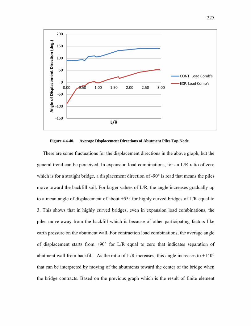
225
Figure 4.4-40. Average Displacement Directions of Abutment Piles Top Node
There are some fluctuations for the displacement directions in the above graph, but the
general trend can be perceived. In expansion load combinations, for an L/R ratio of zero
which is for a straight bridge, a displacement direction of -90° is read that means the piles
move toward the backfill soil. For larger values of L/R, the angle increases gradually up
to a mean angle of displacement of about +55° for highly curved bridges of L/R equal to
3. This shows that in highly curved bridges, even in expansion load combinations, the
piles move away from the backfill which is because of other participating factors like
earth pressure on the abutment wall. For contraction load combinations, the average angle
of displacement starts from +90° for L/R equal to zero that indicates separation of
abutment wall from backfill. As the ratio of L/R increases, this angle increases to +140°
that can be interpreted by moving of the abutments toward the center of the bridge when
the bridge contracts. Based on the previous graph which is the result of finite element
‐150
‐100
‐50
0
50
100
150
200
0.00 0.50 1.00 1.50 2.00 2.50 3.00
Angle of D
isplacem
ent Direction
(deg.)
L/R
CONT. Load Comb's
EXP. Load Comb's

226
analysis of several bridges, approximate smooth curves can be imagined for design
purposes like those displayed in Figure 4.4-41.
Figure 4.4-41. Design Displacement Directions of Abutment Piles Top Node
Using the above graph, the orientation of the abutment piles of the studied bridges is
changed so that the critical displacement of the abutment causes strong-axis bending in
the piles and the models are run again. Orienting the piles for strong-axis bending in the
direction of maximum displacement is based on the results of modeling of straight
bridges in which the direction of displacement was known and strong-axis bending
showed better performance in lowering the stresses. After the analyses, the resulted pile
stresses, which are called optimized stresses, are compared to the stresses of weak-axis
and strong-axis orientation for the piles. For this purpose, the ratios of these stresses to
the optimized stress are calculated and tabulated in Table 4.4-6 and Table 4.4-7:
Eq. 4.53
‐100
‐75
‐50
‐25
0
25
50
75
100
125
150
0.00 0.50 1.00 1.50 2.00 2.50 3.00
Angle of D
irection
(deg.)
L/R
Contraction‐Control
Expansion‐Control

227
L (ft)
R (ft) 308 501 694 887
300 1.00 1.00 1.00 0.89
538 1.06 1.04 1.75 1.56
1000 1.06 1.00 1.40 1.50
Infinity 1.65 1.48 1.60 1.71
Table 4.4-6. Ratio of Piles Weak-axis Orientation Stress to Optimized Stress
L (ft)
R (ft) 308 501 694 887
300 1.19 1.13 1.31 1.12
538 1.23 1.17 1.42 1.31
1000 1.10 1.04 1.00 0.93
Infinity 1.00 1.00 1.00 1.00
Table 4.4-7. Ratio of Piles Strong-axis Orientation Stress to Optimized Stress
As can be seen, in 15 out of 16 bridge models, this method of optimization leads to
stresses less than or equal to the stresses obtained from usual weak-axis or strong-axis
pile orientation stresses. Weak-axis pile orientation which is the most commonly adopted
orientation can cause up to 75% larger stresses and strong-axis orientation can develop
more than 40% greater stresses compared to the optimized solution. So, the presented
method can be put into practice to find the optimal pile orientation for curved integral
abutment bridges. A step by step procedure for this purpose is brought in the following
subsection.

228
B) The Procedure to Find the Optimal Pile Orientation
According to the presented analyses and discussions for optimizing the abutment pile
orientation, the following steps are recommended for design purposes:
Step 1- Using Figure 4.4-38, try to find the critical type of load combinations between
expansion- and contraction-based combinations.
Step 2- Using Figure 4.4-41, find the direction of piles displacement based on the
critical type of load combinations found in Step 1.
Step 3- Orient the strong axis of the abutment piles perpendicular to the displacement
direction found in Step 2.
Step 4- Analyze the bridge based on the recommended pile orientation. Since the
validity of the recommended graph for distinguishing the criticality of expansion versus
contraction is limited to the current study, a more conservative approach is to find the
displacement direction for both expansion-critical and contraction-critical assumptions
and analyze two different models for these two pile orientations and find the optimal
orientation to have the minimum stress in the piles. In the latter procedure, the minimum
stress is guaranteed, even though taking the simpler procedure and trying to find the
critical type of load combinations is much better than choosing the weak- or strong-axis
bending without these considerations.
4.4.4 Effect of Bearing Type and Orientation
There are several types of bearings that are used in bridges. Each type of bearing has
its own characteristics. For example, each type has a specific arrangement for setting the

229
degrees of freedom free, fixed or in between. Since in an integral bridge, the
superstructure is resting on piers by means of a bearing device, it is necessary to study the
effect each bearing type on the responses of the bridge. Different types of bearings and
the status of the degrees of freedom for each of them are tabulated in Table 4.4-8.
Bearing Type Ux
Longitudinal
Uy
Transverse
Uz Rx Ry Rz
Plain or Reinforced Elastomeric k k k k k K
Fixed Pot or Fixed Disc Fix Fix k k k k
Guided Pot or Guided Disc 0 or k Fix k k k k
Sliding (Elastomer or Pot or Disc) 0 0 k k k 0
Rocker or Cylindrical 0 Fix Fix Fix 0 Fix
Spherical Fix Fix Fix 0 0 0
Table 4.4-8. Different Bearing Types and the Associated DOF’s
In this table, “k” means that the DOF has a specific stiffness between zero and infinity.
A free DOF that has zero stiffness and a fixed DOF with a stiffness of infinity are the two
bounds indicated by “0” and “Fix”, respectively.
In the present study, the effects of four different types of bearings which are more
commonly used in integral bridges are studied. These bearings consist of elastomeric,
fixed, guided and sliding bearings. The responses that are studied include the bending
moment of abutment piles and pier columns. For abutment piles, the resultant bending
moment which is the square root of sum of squares of the longitudinal and transverse

230
moments is studied and for the pier columns, the longitudinal and transverse moments are
investigated separately.
A) Effect of Bearing Type on Abutment Pile Moments
To study the effect of different bearing types on the bending moment of abutment
piles, several finite element analyses are conducted on the studied bridges with different
bearings. As there are several load cases applied to the bridges and also several load
combinations, quite a few sets of outputs are resulted. For brevity, only the envelope of
bending moments in different load combinations is presented in Figure 4.4-42.
Figure 4.4-42. Bending Moment of Abutment Piles with Different Bearing Types
In bridges with the radius of 300 feet, the bridges with sliding bearings have larger
moments compared to those with elastomeric, fixed or guided pot bearings. The moments
for the bridges with fixed and guided pot bearings are very close to each other. These two
0
1000
2000
3000
4000
5000
6000
7000
300 400 500 600 700 800 900
Mom
ent (k.in)
Bridge Length (ft)
Maximum Moments in Abutment PilesEnvelope of Load Combinations
R=inf‐Sliding
R=inf‐Elastomer
R=inf‐Guided
R=inf‐Fixed
R300'‐Sliding
R=300'‐Elastomer'
R300‐Guided
R300'‐Fixed

231
types of bearing cause smaller moments in the abutment piles. The other observation on
highly curved bridges is that the maximum abutment pile moment is almost independent
of the length of the bridge. As can be seen, the moment for the bridges with the length of
about 900 feet is approximately equal to the moments in bridges with 300 feet length.
In straight bridges, the general response is similar to that of curved bridges. The
abutment pile moments in bridges with sliding bearings are greater than those in the
bridges with other types of bearings. Fixed and guided pot bearings create slightly
smaller moments compared to the elastomeric bearings, which is attributed to the
restraint that the massive piers have developed against the movements. Abutment pile
moments are increasing as the length of the bridge increases. The other fact is that in
short bridges either curved or straight, the maximum abutment pile moment is
approximately the same for bridges with different types of bearings.
In both straight and curved bridges, the change in the abutment pile moments due to
using different types of bearings is less 20 percent.
B) Effect of Bearing Type on Pier Columns Moments
The moments created in the pier columns are divided into longitudinal and transverse
components that are discussed separately. In this context, the transverse moment means a
moment that causes bending of pier elements in the plane of the pier. The longitudinal
moment causes bending perpendicular to the transverse moment. In the case of curved
bridges, longitudinal moment bends the pier about the radial axis.
The longitudinal moments in straight bridges decrease as the stiffness of the bearing
reduces. It is shown in Figure 4.4-43 that the bridges with fixed bearings have the largest

232
moment values. When the bearings have the properties of elastomers, the moments
decrease and if the bearings are sliding or guided, with sliding direction along the length
of the bridge, the longitudinal moments reduce drastically. In the latter case, the
longitudinal stiffness of the bearings is zero and it may be expected that the moments
should be equal to zero. But, the moments are not equal to zero because of the rotational
stiffness of the bearings. The rotation of the superstructure above the pier and the
rotational stiffness of the bearings build up a moment in the pier in the longitudinal
direction. Another sources of the longitudinal moments can be the loads that are applied
to the pier itself, like wind load if applicable.
In the case of curved bridges, a similar pattern is observed. Bridges with fixed
bearings have the largest moments in the pier columns. If the bearings are elastomeric,
the maximum moment of pier columns reduce compared to those with fixed bearings.
And when the bearings are sliding or guided the moments are considerably smaller.
Figure 4.4-43. Longitudinal Bending Moment of Pier Columns with Different Bearing
Types
0
5000
10000
15000
20000
25000
300 400 500 600 700 800 900
Mom
ent (k.in)
Bridge Length (ft)
Pier Columns Longitudinal Moments
Straight‐FixedPot
Straight‐Elastomer
Straight‐Guided
Straight‐Sliding
R300‐FixedPot
R300‐Elastomer
R300‐Guided
R300‐Sliding

233
The transverse moment of pier columns are plotted versus bridge length for different
radii in Figure 4.4-44. It is observed that curved bridges with fixed bearings have
transverse moments very close to those of the bridges with guided bearings. This is
attributed to the reason presented for the case of abutment piles. If the bearings are
changed to elastomeric ones, the moments drop significantly. In the case of elastomeric
bearing, the transverse moments are on average 60 percent of the moments of bridges
with fixed or guided bearings. If sliding bearings are used, the moments reduce to the
transverse moments that are caused by the pier structure itself, like expansion, contraction
and shrinkage of the pier frame.
In straight bridges, the pier columns transverse moments are mainly due to frame
action of the pier structure, not the behavior of the whole bridge structure. So, it is
generally independent of the bearing type or the length of the bridge. These moments are
very close to the moments if the pier is analyzed alone. The result is that such a pier
configuration itself creates moments about 55000 k.in. In such cases, it can be
recommended that use of massive pier columns in pier bents should be avoided in favor
of multiple slender columns.
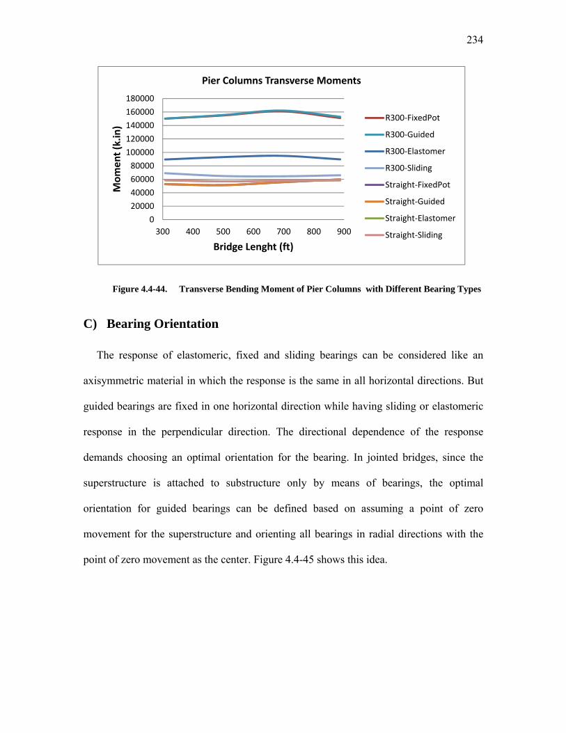
234
Figure 4.4-44. Transverse Bending Moment of Pier Columns with Different Bearing Types
C) Bearing Orientation
The response of elastomeric, fixed and sliding bearings can be considered like an
axisymmetric material in which the response is the same in all horizontal directions. But
guided bearings are fixed in one horizontal direction while having sliding or elastomeric
response in the perpendicular direction. The directional dependence of the response
demands choosing an optimal orientation for the bearing. In jointed bridges, since the
superstructure is attached to substructure only by means of bearings, the optimal
orientation for guided bearings can be defined based on assuming a point of zero
movement for the superstructure and orienting all bearings in radial directions with the
point of zero movement as the center. Figure 4.4-45 shows this idea.
0
20000
40000
60000
80000
100000
120000
140000
160000
180000
300 400 500 600 700 800 900
Mom
ent (k.in)
Bridge Lenght (ft)
Pier Columns Transverse Moments
R300‐FixedPot
R300‐Guided
R300‐Elastomer
R300‐Sliding
Straight‐FixedPot
Straight‐Guided
Straight‐Elastomer
Straight‐Sliding

235
Figure 4.4-45. Guided Bearing Orientation in Jointed Bridges
The presented method for finding the optimal orientation of the bearings is valid
provided that there is no restraint for the bridge movement. If there are some restraints
like fixed bearings or integral abutments, the point of zero movement should be found by
assuming a point as the point of zero movement, orienting the guided bearings along the
rays coming out of that point, analyzing the bridge to find the internal forces of the
elements and optimizing the internal forces by trial and error on the position of the zero
movement point. Figure 4.4-46 shows the rays of alignment for a trail point.
Abut.1 Abut.2
PierAssumed Point ofZero Movement

236
Figure 4.4-46. Guided Bearing Orientation in Bridges with Restraint Superstructure for a
Trial Point
Adopting such an iterative method can be time-consuming if not a waste of time when
there are other bearing types to be used in conjunction with integral bridges. A better
recommendation is to use elastomeric or sliding bearings in the case of integral bridges.
For elastomeric bearings, use of circular bearings is recommended to completely
eliminate the problems arising from bearing direction.
Abut.1 Abut.2
Pier
A Trial Point ofZero Movement
237
Chapter 5
Effect of Curvature on
Concrete IA Bridges
5.1 Introduction
In this chapter, the effect of horizontal curvature on the response of concrete curved
integral abutment bridges is studied. To perform such an investigation, several finite
element models of concrete integral bridges with different lengths and radii of curvature
are analyzed. Each of the studied bridges has a concrete voided slab superstructure, two
integral abutments at the two ends of the bridge and one or more intermediate piers which
their connection to the superstructure is either integral or bearing isolated. All abutments
and piers are supported on concrete piles. More explanations on the modeled bridges are
brought in the following sections. Figure 5.1-1 shows a picture of a concrete curved
integral bridge similar to the bridges that are studied in this section.

238
Figure 5.1-1. A Concrete Curved Integral Bridge Similar to the Studied Bridges
5.2 Bridge Configuration
The components of the studied bridges include superstructure, abutments and piers.
The shape and dimensions of these elements are explained in the following subsections.
5.2.1 Superstructure
In the studied bridges, the superstructure is a concrete voided slab with a total width of
40 feet. This concrete deck consists of two solid concrete side cantilevers of 5 feet length
with the thickness of 12 inches and a voided concrete slab of 44 inches depth. The
diameter of voids is 28 inches and their center to center spacing is 38 inches. Figure 5.2-1
depicts the cross section of the superstructure. As shown in the picture, the bridge has
two curbs at the two sides of the roadway each of them with a width of 24 inches.

239
Figure 5.2-1. Cross Section of the Superstructure of the Modeled Bridges
5.2.2 Abutments
The abutments of the modeled bridges are integrally connected to the superstructure
which is the main characteristic of this type of bridges. Each abutment is consisted of a
50-inch high concrete wall with a thickness of 44 inches which is resting on a row of
three circular concrete shafts. The diameter of each shaft is 40 inches and their length is
50 feet. (In this chapter, the terms shaft and pile are used interchangeably.) As the
thickness of both voided slab and the abutment wall are 44 inches, the connecting zone
has a 44 by 44 square inches cross sectional area which transfers the forces between
superstructure and the abutment.
There are several details for connecting abutments to bridge superstructures integrally,
which can be found in the references. For voided slab superstructures, the integral
connection can be achieved easily by splicing the rebars of the deck and the abutment
28"38"
24" 432 in. = 36 ft. 24"
132" 132" 48" 48" 60" 60"

240
together and casting monolithic concrete for the two adjacent components. Figure 5.2-2
shows such a typical integral connection.
Figure 5.2-2. A Typical Integral Connection for Voided Slab Bridges
5.2.3 Piers
Piers of the modeled bridges consist of three concrete columns of circular cross
section with a radius of 32 inches which are supported on concrete shafts with a diameter
of 48 inches. The length of the columns is 20 feet and the depth of the shaft is 60 feet.
The piers connection to the superstructure is either integral or bearing-isolated. In the
integral connection, the columns are assumed to be rigidly connected to the
superstructure. Figure 5.2-3 illustrates such an integral connection.
D=40"
44"
44"
50"
Drilled ShaftConcrete
Span

241
Figure 5.2-3. Integral Connection of Piers and Superstructure
In the bearing-isolated piers, the columns are connected to each other by means of a
cap beam and the superstructure rests on the cap beam by means of a number of
elastomeric bearings. Figure 5.2-4 shows a typical bearing-isolated superstructure to pier
connection.
Figure 5.2-4. Bearing-Isolated Connection of Piers and Superstructure
132" 132" 48" 48 60" 60"
D=32"Concrete Column
D=48"Drilled ShaftConcrete
L=20'
L=60'
Ground Level
132" 132" 48" 48
D=32"Concrete Column
D=48"Drilled ShaftConcrete
L=17'
L=60'
Ground Level
B=40"Concrete Capbeam
H=32"
Elastomeric Bearing
Pedestal
D=22" T=4"

242
5.3 Finite Element Modeling
In this section, the characteristics of the finite element models that are used to study
the curve concrete integral bridges are explained. These characteristics include the
material properties, the applied loads to the models, soil-structure interaction and the
employed elements.
5.3.1 Material Properties
In the modeled bridges, different components are assumed to be reinforced concrete
elements. The strength of the concrete in different parts varies based on the requirements
of each part.
For all structural elements, the concrete material has a unit weight of 145 lb/ft3, a
coefficient of thermal expansion of 6x10E-6 /degrees F and a Poisson ratio of 0.2.
For voided slab superstructure, concrete columns and the stub abutment walls, the
specified compressive strength of concrete is 5 ksi. The concrete in these parts has a
modulus of elasticity of 4074 ksi and a shear modulus of elasticity of 1698 ksi.
For piles of piers and abutments, the modulus of elasticity of concrete material is equal
to 3644 ksi and the shear modulus is 1518 ksi. For these piles the specified compressive
strength of concrete is 4 ksi.
5.3.2 Loading
In this section, the applied loads to the modeled bridges are reviewed. These loads
include the self weight of the bridge components, the weight of the wearing surface and

243
railing, the effects of live load including gravity, braking and centrifugal forces, the
pressure of soil to the abutments, the thermal loads including expansion, contraction and
temperature gradient through the thickness of superstructure and the effect of concrete
shrinkage. Explanations for each of these loads are presented in the following
subsections.
A) Dead Load (DC)
Assuming a unit weight of 145 / , the dead load is applied to all of the
components of the modeled bridges through calculating the volume of each element.
B) Wearing Surface Load (DW)
Considering a 4-inch thick overlay with a unit weight of 140 / , the weight of
wearing surface is applied to the bridges. In addition to the overlay, two curbs with a
thickness of 12 inches are assumed to exist on the bridges. The weight of railings is
considered to be 67 lb/ft. A schematic picture of the wearing surface components is
shown in Figure 5.3-1.

244
Figure 5.3-1. Wearing Surface of the Modeled Bridges
C) Earth Pressure (EH)
The pressure of the backfill soil is applied to the modeled bridges assuming a
cohesionless soil with a unit weight of 125 / and an angle of internal friction of 30
degrees. Therefore, the soil pressure is:
3.617 10 5
in which is the depth of the soil layer in inches and is the soil pressure in ksi.
Elaborate explanations on how the soil pressure is applied to the structure are presented
in Section 5.3.3 (Soil-Structure Interaction).
D) Live Load (LL)
Live load is applied to the models based on the AASHTO LRFD Bridge Design
Specifications 2010. According to the specifications four different loads should be
considered for such continuous superstructures:
4" OverlayRailing Concrete Curb
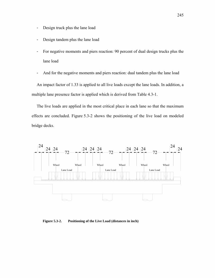
245
- Design truck plus the lane load
- Design tandem plus the lane load
- For negative moments and piers reaction: 90 percent of dual design trucks plus the
lane load
- And for the negative moments and piers reaction: dual tandem plus the lane load
An impact factor of 1.33 is applied to all live loads except the lane loads. In addition, a
multiple lane presence factor is applied which is derived from Table 4.3-1.
The live loads are applied in the most critical place in each lane so that the maximum
effects are concluded. Figure 5.3-2 shows the positioning of the live load on modeled
bridge decks.
Figure 5.3-2. Positioning of the Live Load (distances in inch)
2424 24
72242424
72242424
722424
Wheel Wheel Wheel Wheel Wheel Wheel
Lane Load Lane Load Lane Load

246
E) Braking Force (BR)
As per AASHTO LRFD Bridge Design Specifications, the braking force for each lane
is the maximum of 25 percent of the design truck weight or 5 percent of the design truck
plus lane load weight. This force is calculated for different bridge lengths and applied for
different positions of the live load.
It should be noted that as there are three lanes on the modeled bridges and the
simultaneous braking of the live load of all lanes is considered, a multilane presence
factor, based on Table 4.3-1, is applied to these braking forces. Also, it is noteworthy that
the braking force of each lane for bridges shorter than 450 feet is a constant load equal to
15.3 kips:
72 0.25 0.85 15.3 /
And for longer bridges, it increases with the bridge length as follows:
0.05 72 0.64 0.85 3.06 0.0272 /
F) Centrifugal Force (CE)
When a bridge has horizontal curvature, an important lateral load which is applied to
the bridge superstructure is the centrifugal force of moving loads. Based on AASHTO
LRFD Bridge Design Specification 2010, this radial force is the product of the weight of
design truck or tandem and a factor defined as:
Eq. 5.1
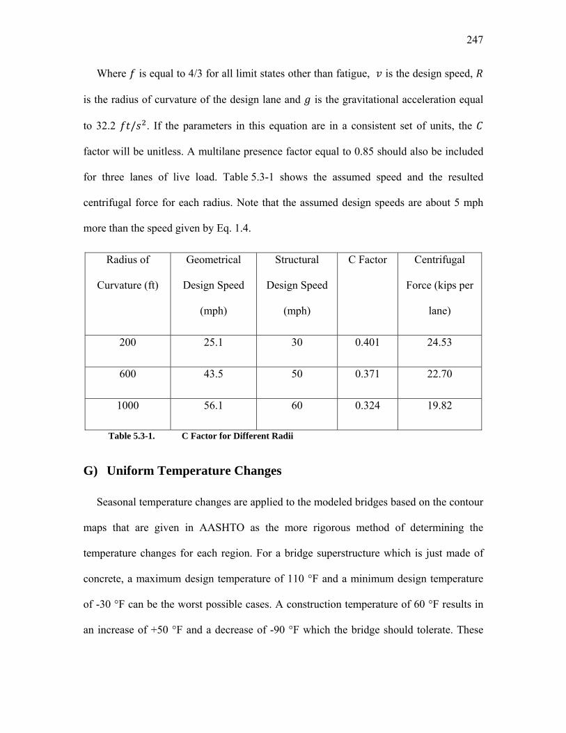
247
Where is equal to 4/3 for all limit states other than fatigue, is the design speed,
is the radius of curvature of the design lane and is the gravitational acceleration equal
to 32.2 / . If the parameters in this equation are in a consistent set of units, the
factor will be unitless. A multilane presence factor equal to 0.85 should also be included
for three lanes of live load. Table 5.3-1 shows the assumed speed and the resulted
centrifugal force for each radius. Note that the assumed design speeds are about 5 mph
more than the speed given by Eq. 1.4.
Radius of
Curvature (ft)
Geometrical
Design Speed
(mph)
Structural
Design Speed
(mph)
C Factor Centrifugal
Force (kips per
lane)
200 25.1 30 0.401 24.53
600 43.5 50 0.371 22.70
1000 56.1 60 0.324 19.82
Table 5.3-1. C Factor for Different Radii
G) Uniform Temperature Changes
Seasonal temperature changes are applied to the modeled bridges based on the contour
maps that are given in AASHTO as the more rigorous method of determining the
temperature changes for each region. For a bridge superstructure which is just made of
concrete, a maximum design temperature of 110 °F and a minimum design temperature
of -30 °F can be the worst possible cases. A construction temperature of 60 °F results in
an increase of +50 °F and a decrease of -90 °F which the bridge should tolerate. These

248
two temperature changes are applied to the modeled bridges as the uniform temperature
loading.
H) Temperature Gradient
The temperature gradient loading is applied to the modeled bridge based on the
provisions of AASSTO Specifications. Assuming a solar radiation zone “1” for the
location of the modeled bridges, a positive temperature gradient of 40 °F is suggested
through the thickness of the superstructure. For the negative temperature gradient, a -0.3
factor should be multiplied to the positive gradient which results in a negative gradient of
-12 °F. These two temperature gradients are also applied to the models.
I) Shrinkage
Concrete shrinkage is a time-dependent volume decrease of the concrete due to loss of
moisture. This phenomenon happens for all concrete elements regardless of presence of
external force on the element. To account for this effect in the models, first the strain due
to concrete shrinkage is calculated and then the equivalent temperature decrease which
causes the same amount of strain is found. In this way, the effect of concrete shrinkage is
simulated.
To calculate the strain in concrete due to shrinkage, the method presented by
AASHTO LRFD 2010 is used. In the code, the shrinkage strain is obtained using the
following equation:
0.48 10 Eq. 5.2

249
For the definition of each of the parameters of Eq. 5.2, the reader is referred to Section
4.3.2J).
Assuming a relative humidity of 70 percent for the location of the bridge under
consideration, a / ratio equal to 0.613 inch, an of 5 ksi for superstructure concrete
and a time of infinity for calculation of the time development factor, the following values
are obtained:
1.45 – 0.13 1.45 0.13 6.44 0.613 1.0 1.0
2 0.014 2 0.014 70 1.02
5
15
1 0.80 5 1.00
61 4 ∞
61 4 4 ∞ 1.0
Having the above factors evaluated, the shrinkage strain can be calculated as:
1.0 1.02 1.0 1.0 0.48 10 490 10
Now the equivalent temperature decrease can be evaluated using the following
equation:
∆
Hence:
6 10 ∆ 490 10
∆ 81.7 °

250
Since in the uniform temperature loading a decrease of -90 °F was considered for
bridge contraction and the equivalent temperature decrease of shrinkage is -81.7 °F, the
effects of the concrete shrinkage can be assumed to be % 90.8 of the effects resulted from
bridge contraction.
5.3.3 Soil-Structure Interaction
The procedure employed to analyze the soil-structure interaction for studied concrete
integral bridges, is similar to what used for steel bridges in Chapter 4. Again, as the
abutment walls separate from the soil under specific loading conditions, but the piles are
surrounded by soil, the soil response is studied in two different subsections for the walls
and piles.
A) Soil-Abutment Interaction
The load-displacement curves of the soil behind the abutment wall of the studied
concrete bridges are derived from the response curves of Figure 4.3-5, presented Clough
and Duncan. For an abutment wall height of 7’-10”, a backfill soil with a unit weight of
125 / 3, an internal friction angle of 30 degrees and for springs of one square foot
tributary area located at different depths, the force-displacement curves of Figure 5.3-3
are obtained which are used in the finite element models.

251
Figure 5.3-3. Force-Displacement Curves of the Abutment Backfill Springs
As the backfill of the bridge abutments are generally composed of granular soils, the
response curve for abutment springs is only presented for cohesionless soils. Therefore,
cohesive soil behavior for abutment backfill is ignored.
B) Soil-Pile Interaction
The response of the soil interacting with shafts of piers or abutments is modeled using
the same technique that was used in steel bridges. The recommendations of American
Petroleum Institute are adopted as the model for the soil behavior (American Petroleum
Institute, 2005). The following subsections describe the resulted load-deflection curves.
B1) Lateral Load-Deflection in Soft Clay
The response of soft clay under lateral loading is generally a nonlinear behavior. API
proposes a p-y curve for short term static loading which may be generated from
Table 4.3-7. In that table, is actual lateral pressure, is the actual lateral deflection,
0.000
0.500
1.000
1.500
2.000
2.500
3.000
3.500
‐5.00 ‐4.00 ‐3.00 ‐2.00 ‐1.00 0.00 1.00 2.00 3.00
Force (kip)
Displacement (in.)
Force‐Displacement Curve for Abutments Springs
Depth=94"
Depth=70"
Depth=46"
Depth=22"
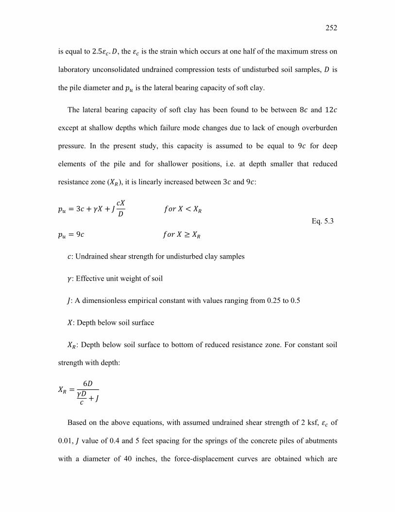
252
is equal to 2.5 . , the is the strain which occurs at one half of the maximum stress on
laboratory unconsolidated undrained compression tests of undisturbed soil samples, is
the pile diameter and is the lateral bearing capacity of soft clay.
The lateral bearing capacity of soft clay has been found to be between 8 and 12
except at shallow depths which failure mode changes due to lack of enough overburden
pressure. In the present study, this capacity is assumed to be equal to 9 for deep
elements of the pile and for shallower positions, i.e. at depth smaller that reduced
resistance zone ( ), it is linearly increased between 3 and 9 :
3
9
Eq. 5.3
: Undrained shear strength for undisturbed clay samples
: Effective unit weight of soil
: A dimensionless empirical constant with values ranging from 0.25 to 0.5
: Depth below soil surface
: Depth below soil surface to bottom of reduced resistance zone. For constant soil
strength with depth:
6
Based on the above equations, with assumed undrained shear strength of 2 ksf, of
0.01, value of 0.4 and 5 feet spacing for the springs of the concrete piles of abutments
with a diameter of 40 inches, the force-displacement curves are obtained which are

253
plotted in Figure 5.3-4. As can be observed, the behavior for the springs deeper than 33
feet, is independent of the depth of the soil. This constant response is applicable to
springs down to the end of the piles which are 50 feet deep.
Figure 5.3-4. Force-Displacement Curves of the Springs of Piles of Abutments in Soft Clay
For the response of the soil neighboring the pile of piers which have a diameter of 48
inches, assuming the same constants and soil properties as for abutment piles, the curves
of Figure 5.3-5 are derived. As can be seen, from the depth of 36.9 feet to the end of the
piles, which is the depth of 65 feet, the reaction of the soil does not change.
‐400
‐300
‐200
‐100
0
100
200
300
400
‐15 ‐10 ‐5 0 5 10 15Force (kip)
Displacement (in.)
Force‐Displacement of Abutment Pile Springs
Depth>32.86 ft
Depth=20 ft
Depth=10 ft

254
Figure 5.3-5. Force-Displacement Curves of the Springs of Piles of Piers in Soft Clay
B2) Lateral Load-Deflection in Sand
API recommends a hyperbolic tangent equation for the lateral force-displacement
curve of the piles in sand as follows:
. . . tanh
Eq. 5.4
Where:
: Lateral soil resistance in a length of of pile (force)
: An empirical correction factor, 3 0.8 0.9
: Estimated ultimate lateral soil resistance (force/unit length)
: Length of the pile section
: Initial modulus of subgrade reaction from Figure 4.3-9
: Soil depth from the top of the soil layer
‐400
‐300
‐200
‐100
0
100
200
300
400
‐20 ‐15 ‐10 ‐5 0 5 10 15 20Force (kip)
Displacement (in.)
Force‐Displacement of Pier Pile Springs
Depth>36.9 ft
Depth=20 ft
Depth=10 ft

255
: Displacement in the horizontal direction
The ultimate soil lateral resistance can be obtained based on the given equations as the
minimum of:
. . Eq. 5.5
And
. . . Eq. 5.6
Where:
: Ultimate sand lateral resistance at shallow depths (force/unit length)
: Ultimate sand lateral resistance at deep depths (force/unit length)
: Pile Diameter
: Effective soil density
: Angle of internal friction
45
1
/2
45
: Active earth pressure coefficient
: At-rest earth pressure coefficient

256
The values of constants , and can be found from Figure 4.3-10. This figure
may also be used to check the values obtained from the relevant equations.
Using the above equations and considering a diameter of 48 inches for the shafts of
piers, a soil unit net weight of 125 / , an angle of internal friction of 30 degrees and
five feet spacing for the springs, a k value of 45 lb/in3 is obtained from Figure 4.3-9
which results in the force-displacement curves of Figure 5.3-6 for the pile springs. As
shown in the Figure 5.3-6, the force-displacement curves strongly depend on the depth of
the springs.
Figure 5.3-6. Force-Displacement Curves of the Springs of Piles of Piers in Sand
The response of the springs of the piles of the abutments can be plotted by employing
the same values as used for the pier piles in the related equations and considering a
‐5000
‐4000
‐3000
‐2000
‐1000
0
1000
2000
3000
4000
5000
‐6 ‐4 ‐2 0 2 4 6
Force (kip)
Displacement (in.)
Force‐Displacement of Pier Pile Springs
Depth=13 ft
Depth=26 ft
Depth=39 ft
Depth=52 ft
Depth=65 ft

257
diameter of 40 inches for the piles. Figure 5.3-7 shows the force-displacement curves for
these springs.
Figure 5.3-7. Force-Displacement Curves of the Springs of Piles of Abutments in Sand
5.3.4 Elements
The bridges studies in this chapter consist of voided slab superstructures, flexible
integral abutments interacting with the backfill soil and the surrounding soil of the piles
and some piers comprising concrete columns and piles. The piles of the piers are also in
contact with the supporting soil. As can be observed, the bridge behavior is controlled by
several structural elements that need different elements to be used for better modeling.
An explanation of these finite elements is brought in the following subsections.
‐3000
‐2000
‐1000
0
1000
2000
3000
‐6 ‐4 ‐2 0 2 4 6
Force (kip)
Displacement (in.)
Force‐Displacement of Abutment Pile Springs
Depth=10 ft
Depth=20 ft
Depth=30 ft
Depth=40 ft
Depth=50 ft

258
A) Beam Element
To model the pier columns and also the piles of the piers and abutments, two-node
frame elements are used. For description of the beam elements refer to the Section
4.3.5A).
B) Shell Element
The superstructure including the voided slab deck and the side cantilevers and also the
stub abutments of the bridges are modeled using shell elements. A shell element is a
three- or four-node formulation which combines membrane and plate behaviors. For
more complete description of the shell elements refer to Section 4.3.5B).
C) Nonlinear Link Element
Nonlinear link elements are used to connect two joints together with specified
nonlinear properties. As explained in Chapter 3, each link element may have three
different types of behavior based on the required properties and the analysis type. These
properties include: linear, nonlinear and frequency-dependent.
In the modeled bridges, these link elements are used to simulate the elastomeric
bearings connecting the piers to the superstructure. In design of the elastomeric bearings,
it is assumed that the area of the bearing should be chosen so that the pressure on the
bearing is not less than a specified value, namely one third or one fourth of the maximum
allowed pressure on the bearing. This assumption yields to the fact that these types of
bearings shall be not in tension in any of the load combinations. On the other hand, as the
maximum applied pressure on the neoprene is limited by the manufacturers (typically to
2 ksi), the stiffness of the link element in the six degrees of freedom can be determined as

259
follows. In the following equations, the gravity direction of the neoprene is assumed as
direction 1 and the two shearing directions are assumed as 2 and 3. For a circular
elastomeric bearing of 22-inch diameter and 4-inch thickness, assuming an elastic
modulus of 85.3 ksi and a shear modulus of 0.142 ksi, the following stiffnesses can be
calculated:
Axial stiffness:
85.3 4 22
4 8106 /
Shearing stiffness:
0.142 4 22
4 13.5 /
Torsional stiffness:
0.142 32 22
4 816 . /
Bending stiffness:
85.3 64 22
4 245216 . /
Where:
is the cross sectional area, is axial modulus of elasticity, is the total thickness
including rubber and steel plates, is the shear modulus of elasticity, is the torsional
constant (equal to for circular neoprenes) and is the moment of inertia of the section
of the elastomeric bearing.

260
Therefore, the calculated stiffness of the bearings are entered into the finite element
model. A picture of the elastomeric bearing modeling of a pier of the modeled bridges is
shown in Figure 5.3-8.
Figure 5.3-8. Modeling of the Elastomeric Bearings
D) Nonlinear Support Element
To model the effect of the soil support which acts on the abutment walls and the
surface of the piles, nonlinear support elements are used. These elements are one-node
grounded nonlinear springs.
As two different types of properties are supposed to be analyzed with these elements
which are soil-abutment interaction and soil-pile interaction, two different sets of
properties are defined for these elements.

261
The first set of assigned properties to nonlinear support elements is based on the force-
displacement curves of Figure 5.3-3 which are assigned to the nonlinear springs of the
abutment walls.
The second set of assigned properties to nonlinear springs is based on the force-
displacement curves of Figure 5.3-4 and Figure 5.3-5 which are considered for the
springs that are supposed to model the behavior of the surrounding soil of the shafts of
abutments and piers. As the shafts are embedded in the soil, the springs have the same
nonlinear response in tension and compression.
5.3.5 Finite Element Models
Based on the information provided in the previous sections, a comprehensive finite
element analysis study is conducted. In the analyses, the movements and internal forces
of curved integral abutment bridges are evaluated and compared to the responses of
straight bridges.
In order to perform such analyses, several finite element models of curved bridges
with radius of curvature equal to 200, 600 and 1000 feet are made. For each of these
radii, the bridge is modeled in different lengths, namely 130, 215, 300, 470 and 640 feet.
On the other hand, the equivalent straight bridge of each curved model is simulated with
exact same characteristics as the curved bridge except the curvature. The length of the
end spans and intermediate spans of the studied bridges are 65 and 85 feet, respectively.
As shown before, the width of all the bridges is 40 feet. Figure 5.3-9 illustrates a typical
finite element model that is made in this study.

262
Figure 5.3-9. A Typical Finite Element Model of the Studied Bridges
5.4 Results of FE Analysis
In this section, the results of the previously explained finite element analyses are
presented. To comprehend the behavior of curved concrete integral bridges, different
problems are discussed. First, the internal forces of the abutment piles are studied and
compared to counterpart straight bridges. The results are presented for a variety of load
cases that were discussed in Section 5.3.2. Integral bridges can have bearing-isolated
rigid piers or flexible integral piers. The responses in these two types of structures are
compared. The other part of this section focuses on the integral piers. When the piers are
integrally connected to superstructure, they should be flexible to accommodate the
movements. And flexibility requires slender columns to be incorporated in the structure.
The superiority of adopting integral bridge systems when slender columns are needed is
then discussed.

263
5.4.1 Effect of Length and curvature on Load
Responses
In this section, the consequences of variation in the bridge length and curvature on the
load effects are presented. In the design of integral abutment bridges, the most critical
response is the internal forces in abutment piles. In most cases, the pile forces determine
the maximum possible bridge length. Other responses like the bending moments in the
superstructure, the moments in the abutment concrete wall can be designed by choosing
larger sections or stronger material. The axial forces in the piles can also be designed
choosing enough long piles. Therefore, the study is narrowed down to the flexural forces
of the abutment piles which are discussed in the following sections.
A) Bending Moment of Abutment Piles
Abutments of the modeled bridges are comprised of the stub wall and the piles. The
height of the stub wall is just 50 inches and it is a continuous element compared to
discrete supporting piles. Therefore, from a structural design point of view, the piles are
more critical for design. This statement is more clarified noting the fact that the
summation of the bending moments of the stub wall and the piles along the line of their
intersection are equal. For the wall, this moment is distributed along the horizontal length
of the wall which is 40 feet, but for the piles, the moment is divided among the piles, in
this case among three piles. Hence, to study the variation of the internal forces of the
abutments, those of the abutment piles are investigated.
A1) Contraction

264
The flexural moments of the abutment piles of the modeled bridges are evaluated
using the finite element program for both curved and straight bridges under bridge
contraction loading. These moments are plotted versus the length of the bridges in
Figure 5.4-1. It is observed that for straight bridges the moment blows up as the length
increases. In curved bridges the rate of increase in the moments reduces as the curvature
increases. In highly curved bridges, the moments have a drastic decrease as the length of
the bridge gets larger. For a radius of 200 feet, the moment in a bridge of 640 feet is
smaller than that of a bridge with 130 feet length.
Figure 5.4-1. Maximum Moment of Abutment Piles Due to Contraction
A2) Expansion
The bending moment of abutment piles due to straight bridge expansion increases
strictly as the length of the bridge increases. In curved bridges, the moment increases up
0
5000
10000
15000
20000
25000
100 200 300 400 500 600 700
Mom
ent (k.in)
Bridge Length (ft)
Concrete Integral Abutment Bridges
R=infinity
R=1000'
R=600'
R=200'

265
to a specific length at which a maximum moment occurs. The length corresponding to the
maximum moment depends on the curvature, ranging from 300 feet for a radius of 200
feet to 500 feet for a radius of 1000 feet. For longer bridges the moments start to reduce.
Figure 5.4-2. Maximum Moment of Abutment Piles Due to Expansion
A3) Live Load
For each radius, the pile moments due to live load have an increase as the length of the
bridge increases from 130 feet (two-span bridge) to 300 feet (four-span bridge). For
longer bridges, it is almost constant. The response for straight bridges and curved bridges
with the radius of 1000 feet are very close. For a radius of 600 feet, the moments are
larger than the other bridges.
0
1000
2000
3000
4000
5000
6000
7000
100 200 300 400 500 600 700
Mom
ent (k.in)
Bridge Length (ft)
Concrete Integral Abutment Bridges
R=infinity
R=1000'
R=600'
R=200'
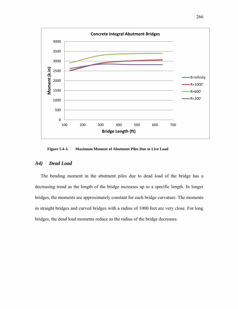
266
Figure 5.4-3. Maximum Moment of Abutment Piles Due to Live Load
A4) Dead Load
The bending moment in the abutment piles due to dead load of the bridge has a
decreasing trend as the length of the bridge increases up to a specific length. In longer
bridges, the moments are approximately constant for each bridge curvature. The moments
in straight bridges and curved bridges with a radius of 1000 feet are very close. For long
bridges, the dead load moments reduce as the radius of the bridge decreases.
0
500
1000
1500
2000
2500
3000
3500
4000
100 200 300 400 500 600 700
Mom
ent (k.in)
Bridge Length (ft)
Concrete Integral Abutment Bridges
R=infinity
R=1000'
R=600'
R=200'
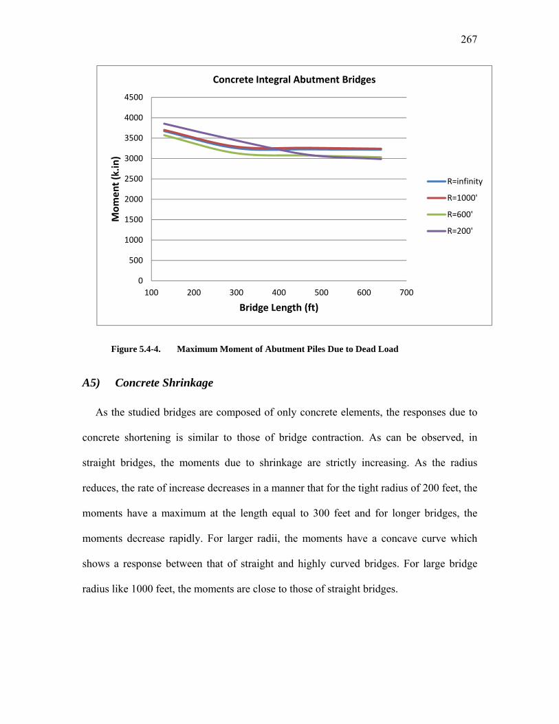
267
Figure 5.4-4. Maximum Moment of Abutment Piles Due to Dead Load
A5) Concrete Shrinkage
As the studied bridges are composed of only concrete elements, the responses due to
concrete shortening is similar to those of bridge contraction. As can be observed, in
straight bridges, the moments due to shrinkage are strictly increasing. As the radius
reduces, the rate of increase decreases in a manner that for the tight radius of 200 feet, the
moments have a maximum at the length equal to 300 feet and for longer bridges, the
moments decrease rapidly. For larger radii, the moments have a concave curve which
shows a response between that of straight and highly curved bridges. For large bridge
radius like 1000 feet, the moments are close to those of straight bridges.
0
500
1000
1500
2000
2500
3000
3500
4000
4500
100 200 300 400 500 600 700
Mom
ent (k.in)
Bridge Length (ft)
Concrete Integral Abutment Bridges
R=infinity
R=1000'
R=600'
R=200'

268
Figure 5.4-5. Maximum Moment of Abutment Piles Due to Concrete Shrinkage
A6) Horizontal Earth Pressure (EH)
The abutment pile moments are approximately constant for straight bridges. In this
case, there is a slight increase in moments for longer bridges as depicted in Figure 5.4-6.
For radius equal to 600 and 1000 feet, the response is similar to straight bridges with a
larger increase as the length increases. For highly curved bridges, R=200 feet, the
response is totally different. The moments increase rapidly as the radius decreases from
600 feet to 200 feet. The reason is illustrated in Figure 5.4-7 through Figure 5.4-9. In a
straight bridge, the earth forces are in the same line and opposite to each other. Therefore,
they balance each other and only cause local bending in the piles. In a tightly curved
bridge depending on the length-to-radius ratio, the earth pressures are not counteracting
like in straight bridges. For small Length/Radius ratios the major components of earth
0
2000
4000
6000
8000
10000
12000
14000
16000
100 200 300 400 500 600 700
Mom
ent (k.in)
Bridge Length (ft)
Concrete Integral Abutment Bridges
R=infinity
R=1000'
R=600'
R=200'

269
pressure balance each other. But for large Length/Radius ratios, the earth pressure is
mainly resisted by the internal forces in the structure. In some cases, as shown in
Figure 5.4-7, the earth pressure may be almost perpendicular to each other. In such
situations, large lateral displacements occur due to earth pressure which results in large
bending moments in the abutment piles.
Figure 5.4-6. Maximum Moment of Abutment Piles Due to Horizontal Earth Pressure
0
200
400
600
800
1000
1200
1400
1600
100 200 300 400 500 600 700
Mom
ent (k.in)
Bridge Length (ft)
Concrete Integral Abutment Bridges
R=infinity
R=1000'
R=600'
R=200'

270
Figure 5.4-7. Plan View of Deformed Shape of the Bridge with R=200’ under EH
Figure 5.4-8. Plan View of Deformed Shape of the Bridge with R=600’ under EH

271
Figure 5.4-9. Plan View of Deformed Shape of the Bridge with R=1000’ under EH
A7) Centrifugal Force
Figure 5.4-10 describes the pile moments due to centrifugal forces. It shows that the
centrifugal moments are larger for short bridges. Up to a length of 400 feet, the moments
are decreasing and for longer bridges, the moments are constant.

272
Figure 5.4-10. Maximum Moment of Abutment Piles Due to Centrifugal Force
A8) Weight of Wearing Surface
The changes in moments due the weight of wearing surface are similar to those of
dead load. In general, there is a decreasing trend in the moments as the length increases.
The response of bridges with the radius equal to 1000 feet is very close to that of straight
bridges.
0
200
400
600
800
1000
1200
1400
1600
1800
100 200 300 400 500 600 700
Mom
ent (k.in)
Bridge Length (ft)
Concrete Integral Abutment Bridges
R=infinity
R=1000'
R=600'
R=200'

273
Figure 5.4-11. Maximum Moment of Abutment Piles Due to Weight of Wearing Surface
A9) Braking Force
The pile moments because of braking force are shown in Figure 5.4-12. It is observed
that the moments increase as the radius of the bridge decreases. This is mainly attributed
to the balance of braking force by the backfill pressure. In straight bridges or those with a
large radius, the braking force is resisted by the passive pressure of the abutment backfill.
But, in highly curved bridges, a large component of the braking force is not balanced by
the earth pressure and creates a large bending moment is abutment piles and piers. The
other fact is the increase in the slope of the curves for bridges longer than 450 feet. This
is because of the change in the magnitude of braking force in the design code for bridges
beyond this length.
0
100
200
300
400
500
600
700
800
900
100 200 300 400 500 600 700
Mom
ent (k.in)
Bridge Length (ft)
Concrete Integral Abutment Bridges
R=infinity
R=1000'
R=600'
R=200'

274
Figure 5.4-12. Maximum Moment of Abutment Piles Due to Braking Force
A10) Positive Temperature Gradient
It is shown in Figure 5.4-13 that the bending moments due to positive temperature
gradient is approximately constant as the length of the bridge changes. Also, it is
observed that these moments reduce as the radius of the bridge decreases. The difference
in the moments between straight bridges and those with radius equal to 200 feet is less
than 20 percent. So, as an estimate, it can be assumed that the moments due to
temperature gradient are independent of bridge length and radius.
0
200
400
600
800
1000
1200
100 200 300 400 500 600 700
Mom
ent (k.in)
Bridge Length (ft)
Concrete Integral Abutment Bridges
R=infinity
R=1000'
R=600'
R=200'

275
Figure 5.4-13. Maximum Moment of Abutment Piles Due to Positive Temperature
Gradient
A11) Negative Temperature Gradient
As negative temperature gradient is equal to minus 30 percent of the positive one, the
results pattern is similar to that of positive gradient. For description of the results, the
reader is referred to the previous section.
0
500
1000
1500
2000
2500
3000
3500
4000
4500
100 200 300 400 500 600 700
Mom
ent (k.in)
Bridge Length (ft)
Concrete Integral Abutment Bridges
R=infinity
R=1000'
R=600'
R=200'

276
Figure 5.4-14. Maximum Moment of Abutment Piles Due to Negative Temperature
Gradient
A12) Combination of the Loads
The final plot for load effects, and the most important one, is illustrated in Figure 5.4-
15. The envelopes of the maximum bending moments in different load combinations are
shown in this picture. The significant observation is that in curved bridges, the envelope
moments are not strictly increasing. In highly curved bridges with radius equal to 200
feet, the moments are almost constant for bridges longer than 300 feet. In bridges with
larger radius, the moments are between those of R=200 and straight bridges. The bridges
with R=1000 feet have moments very close to straight bridges, so that these moment can
be estimate ignoring the effect of curvature.
0
200
400
600
800
1000
1200
1400
100 200 300 400 500 600 700
Mom
ent (k.in)
Bridge Length (ft)
Concrete Integral Abutment Bridges
R=infinity
R=1000'
R=600'
R=200'
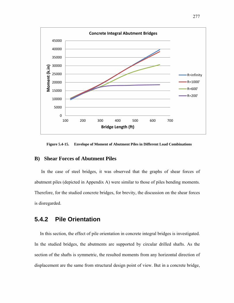
277
Figure 5.4-15. Envelope of Moment of Abutment Piles in Different Load Combinations
B) Shear Forces of Abutment Piles
In the case of steel bridges, it was observed that the graphs of shear forces of
abutment piles (depicted in Appendix A) were similar to those of piles bending moments.
Therefore, for the studied concrete bridges, for brevity, the discussion on the shear forces
is disregarded.
5.4.2 Pile Orientation
In this section, the effect of pile orientation in concrete integral bridges is investigated.
In the studied bridges, the abutments are supported by circular drilled shafts. As the
section of the shafts is symmetric, the resulted moments from any horizontal direction of
displacement are the same from structural design point of view. But in a concrete bridge,
0
5000
10000
15000
20000
25000
30000
35000
40000
45000
100 200 300 400 500 600 700
Mom
ent (k.in)
Bridge Length (ft)
Concrete Integral Abutment Bridges
R=infinity
R=1000'
R=600'
R=200'

278
the shafts can be asymmetric, like rectangular shafts, or the rebars in a symmetric shaft
can be asymmetric. Then, different orientations of the shafts result in different internal
forces. Therefore, there should be a criterion to determine the optimum orientation of the
shafts.
To study this problem, the circular piles of the studied concrete bridges are replaced
by rectangular shafts. The shafts have a 40-inch by 20-inch cross section. Two sets of
finite element models are made with strong-axis and weak-axis bending orientations for
the piles. The bridges are analyzed with these two shaft orientations to find the internal
forces of the shafts including the axial force and bending moments. The results for the
bridge with the length of 130 feet are shown in Table 5.4-1:
Orientation Axial Force
(kip)
M22 (weak axis
moment) (k.in)
M33 (strong axis
moment) (k.in)
Weak-Axis
Bending 105 863 9381
Strong-Axis
Bending 105 1143 8492
Table 5.4-1. Internal Forces of Shafts with Different Orientations
The shafts are designed by the program PCACOL to calculate the required rebar area
in each of them. The results show that for the strong-axis orientation of the shafts, 8.22
square inches of Grade 60 rebar is requires. This area of rebar is equal to 1.025 percent of
the gross cross sectional area of the shaft. Figure 5.4-16 and Figure 5.4-17 depict the
design details in the program format. The shaft with weak-axis orientation is also

279
designed for the resulted internal forces. The needed area of Grade 60 rebar for the weak-
axis bending is 16.56 square inches. It is equivalent to 2.07 percent of the gross cross
sectional area of the shaft. The details of the design process are shown in Figure 5.4-18
and Figure 5.4-19.
Therefore, it is concluded that the strong-axis bending of the drilled shafts results in
more economical designs in the case of straight bridges. A similar conclusion was made
for the orientation of steel piles in the previous chapter.

280
Figure 5.4-16. PCACOL Design Sheet for Strong-Axis Orientation (1 of 2)

281
Figure 5.4-17. PCACOL Design Sheet for Strong-Axis Orientation (2 of 2)

282
Figure 5.4-18. PCACOL Design Sheet for Weak-Axis Orientation (1 of 2)

283
Figure 5.4-19. PCACOL Design Sheet for Weak-Axis Orientation (2 of 2)

284
5.4.3 Bearing-Isolated Pier vs. Flexible Integral Pier
As described in the Section 5.2.3, there can be two different types of piers in the
studied concrete integral bridges. In one of the pier types, the columns of the pier are
integrally connected to the superstructure. As both columns and superstructure are
concrete elements, just extending the rebars of the columns into the superstructure with
the required development length provides the integrity of the piers and superstructure. In
the second type of piers, the pier columns and a cap beam form a frame which the
superstructure seats on it by means of elastomeric bearings. Therefore, a large amount of
the movements of the superstructure can be accommodated by bearings instead of the
pier structure. Figure 5.2-3 and Figure 5.2-4 describe these two types of piers graphically.
The concrete integral abutment bridges are analyzed with these two types of piers. As
the stiffnesses of these two piers are not the same, the internal forces of the structures are
different. The point of interest in the design of integral abutment bridges is the abutment
piles. The envelope of flexural moment of abutment piles in different load combinations
are derived from the finite element models and plotted versus different bridge lengths in
Figure 5.4-20. As can be observed, in straight bridges, the difference between the pile
moments with different pier types is ignorable. In curved bridges, the pile moments in the
bridges with integral piers are greater than those of bridges with isolated piers. As the
radius of curvature of the bridges is reduced, the difference between the moments is more
profound. The largest change in the moments is for bridges with the radius equal to 200
feet which a 15 percent reduction is observed when the piers are bearing-isolated.

285
Figure 5.4-20. Envelope of Moment of Abutment Piles in Different Load Combinations in
Bridges with Integral Piers vs. Bridges with Elastomeric Isolated Piers
5.4.4 Mitigation of Moment Magnification
In design of frames, the second order ∆ effects should be taken into account. The
studied concrete integral abutment bridges which have integral piers are 3D frames. Such
bridges have an enhanced ∆ behavior compared to jointed bridges. In this section, the
difference between the behavior of these two types of bridges and the superiority of
integral abutment designs are explained.
To design the columns of the piers of a jointed bridge, the flexural moments of the
columns should be determined from a second order elastic analysis or an approximate
procedure as follows (American Institute of Steel Construction, American Institute of
Steel Construction, & Manual of steel construction, 2005):
0
5000
10000
15000
20000
25000
30000
35000
40000
45000
100 200 300 400 500 600 700
Mom
ent (k.in)
Bridge Length (ft)
Maximum Moments in Abutment PilesEnvelope of Load Combinations
Integral Pier vs. Bearing Isolated Pier
R=infinity‐Integral
R=infinity‐Elastomer
R=1000'‐Integral
R=1000'‐Elastomer
R=600'‐Integral
R=600'‐Elastomer
R=200'‐Integral
R=200'‐Elastomer
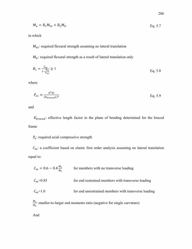
286
Eq. 5.7
in which
: required flexural strength assuming no lateral translation
: required flexural strength as a result of lateral translation only
1 Eq. 5.8
where
Eq. 5.9
and
: effective length factor in the plane of bending determined for the braced
frame
: required axial compressive strength
: a coefficient based on elastic first order analysis assuming no lateral translation
equal to:
0.6 0.4 for members with no transverse loading
=0.85 for end restrained members with transverse loading
=1.0 for end unrestrained members with transverse loading
: smaller-to-larger end moments ratio (negative for single curvature)
And
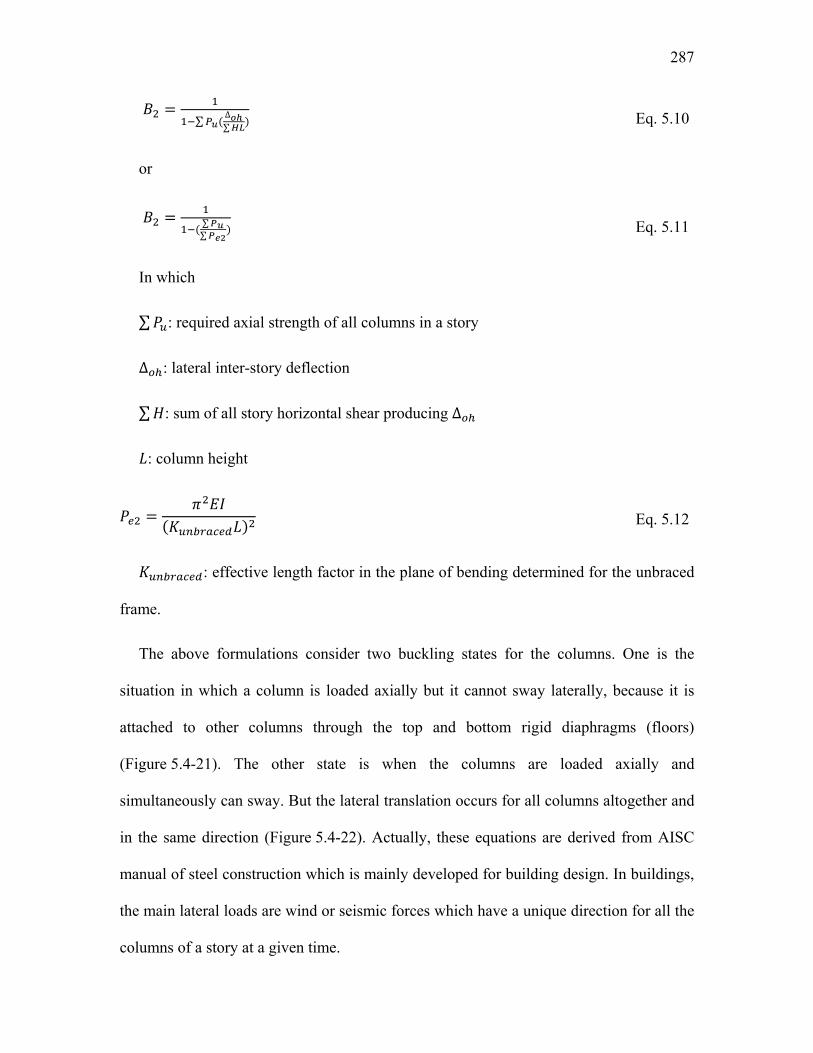
287
∑ ∆
∑
Eq. 5.10
or
∑∑
Eq. 5.11
In which
∑ : required axial strength of all columns in a story
∆ : lateral inter-story deflection
∑ : sum of all story horizontal shear producing ∆
: column height
Eq. 5.12
: effective length factor in the plane of bending determined for the unbraced
frame.
The above formulations consider two buckling states for the columns. One is the
situation in which a column is loaded axially but it cannot sway laterally, because it is
attached to other columns through the top and bottom rigid diaphragms (floors)
(Figure 5.4-21). The other state is when the columns are loaded axially and
simultaneously can sway. But the lateral translation occurs for all columns altogether and
in the same direction (Figure 5.4-22). Actually, these equations are derived from AISC
manual of steel construction which is mainly developed for building design. In buildings,
the main lateral loads are wind or seismic forces which have a unique direction for all the
columns of a story at a given time.

288
Figure 5.4-21. ∆ Effect in Non-Sway Mode
Figure 5.4-22. ∆ Effect in Sway Mode
In bridges in addition to the above two situations, one more state can happen. Consider
a three-span bridge jointed at the abutments. When the bridge is under uniform thermal
loads, for example contraction, the top of the columns move toward the center of the
bridge (or more exactly toward the point of zero movement). The critical case takes place
when the axial force of one of the columns is maximized due to presence of live load.
Figure 5.4-23 shows a bridge in such a state. Under such circumstances, the moment in
the loaded columns (left columns in the picture) tends to magnify. But, as the ∆ and
moments increase in this column, the other column tends to restore to its undeformed

289
shape. Therefore, the assumption in the building structures which a floor moves in a
unique direction due to a loading case is not valid for bridge under the described
conditions. In building structures, the terms such as ∑ or ∑ are based on the
assumptions that are valid only for that type of structure.
Figure 5.4-23. ∆ Effect in a Jointed Abutment Bridge with Flexible Piers
For bridge design, more critical conditions in which an axially loaded column can
have a side sway while other columns do not have the same direction of side sway should
be considered. In this case, the other columns, not only do not help the column that has
the maximum axial load, but also they may act like springs that intensify the ∆ effect for
the critical column. Therefore, the following magnification factor may be recommended
for a column in such a situation.
,
1 Eq. 5.13
where
, Eq. 5.14

290
In integral abutment bridges, as the two ends of the bridge are connected to the
abutments, for movement in any direction at least one of the abutments is a help for the
intermediate columns. Figure 5.4-24 illustrates an integral abutment bridge under such a
situation. As can be observed, the stiffness of the left abutment piles mitigates the
moment magnification of the axially loaded columns. For this case, the following
equation for the magnification factor can be recommended, in which the resisting
elements are the left abutment and left pier.
∑ ,∑ ,
Eq. 5.15
In which
, Eq. 5.16
Figure 5.4-24. ∆ Effect in an Integral Abutment Bridge with Flexible Piers

291
Chapter 6
Concluding Remarks and
Future Research
The concluding remarks of the present study are divided into three sections. First, the
findings of the close-up analysis of the integral abutment connections are summarized.
Then, the conclusions of the investigations on steel I-girder bridges are explained. After
that, the results of the studies on concrete bridges are recapitulated. At the end, some
recommendations for future research are presented.
6.1 Connections of Integral Abutments
An important part of the current study was to investigate the behavior of abutment
connections in steel integral bridges. Each integral abutment has two connection zones:
one is the superstructure-to-abutment wall connection and the other is the pile-to-
abutment wall connection. The state of stresses in each of these two connections has been
scrutinized.
For the girder-to-abutment wall connection, it was observed that the girder stresses in
the vicinity of the wall face are mainly concentrated in the lower part of the girder web.

292
This means that the maximum stresses are not found in the bottom flange of the girder.
This is attributed to the mechanism of stress transfer between the steel girder and the
neighboring concrete wall. The effect of adding a stiffener to the girder web at the section
of the wall face has also been studied. The results show that the stiffener is effective in
spreading the stresses over the face of the concrete wall below the bottom flange. This
had a minor effect on the stresses of the girder itself. Another idea that was studied was to
add shear studs to the bottom flange of the girder for the length embedded in the wall. It
was observed that shear studs did not change the maximum stresses of the girder, but
were effective in reducing the concrete wall stresses by about 40 percent.
The second zone which has been studied is the pile-to-abutment wall connection. For
this zone the significant observation is the high stresses in the steel pile, so that the pile
section is almost fully plastic. The stresses in the concrete abutment wall are also high,
even higher than the characteristic strength, which can be interpreted as the confinement
effects. The effect of stiffener on the stresses in the pile and concrete wall was also
examined. It was concluded that the pile stiffener reduces the maximum stresses on the
face of the wall. This stiffener is not as effective as the stiffener for the girder-to-wall
connection because of different load transfer configurations.
6.2 Steel I-girder IA Bridges
Several integral steel I-girder bridges were studied in this dissertation. The baseline
model for the analyses was the I-480 Bridge in Omaha, NE, which is a four-span
composite steel I-girder bridge with a radius of 538 feet. Several other models were
generated based on this bridge for various bridge lengths and radii. The bridges were

293
analyzed using finite element models. Full 3D finite element analysis was conducted
including the modeling of girder flanges and web plates, concrete deck slab, shear studs,
cross frames, stiffener plates, different bearing connections, pier caps, non-prismatic
columns, pile caps, pier H-piles, abutment walls, abutment piles and even parapets. Based
on the need, different elements such as solid, shell, plate and beam elements are
employed. The soil-structure interaction has been modeled as well. A wide variety of
loads and load effects have been applied to the models including dead load, live load,
centrifugal force, braking force, earth pressure, uniform temperature changes,
temperature gradient, wind load and concrete shrinkage.
6.2.1 Effects of Bridge length and curvature on load
responses
Based on the results of the analysis for different loads, a weight factor is defined for
each load. The larger weight factor for a specific load means the larger internal forces due
to that load. Therefore, a larger weight factor indicates the importance of the loading
from a structural design point of view. The sorting of the loads based on their weight
factors is as follows: contraction, expansion, live load, wind load, dead load, concrete
shrinkage, horizontal earth pressure, centrifugal force, weight of wearing surface, braking
force, positive temperature gradient and finally negative temperature gradient.
The results of the study show that the internal forces in the abutments of curved
bridges due to contraction loading, which is the most critical loading for design purposes,
are always smaller than those of straight bridges. As the radius of curvature of the bridge
reduces, the internal forces reduce as well. Besides, the increase in the length of straight

294
or large-radius bridges increases the internal forces of the abutment piles. But for smaller
radii, the abutment piles’ internal forces start to decrease as the bridge is longer than a
specific length.
For bridge expansion, the results show that in straight bridges the internal forces
increase as the length of the bridge increases. But, in the case of curved bridges, there is
an increase in the responses for shorter bridges and then the curves reach a maximum
point. For longer bridges beyond the maximum point, the internal forces are decreasing.
Therefore, it can be concluded that the internal forces due to expansion for bridges longer
than a specific length are smaller than those of straight bridges. That specific length
depends mainly on bridge curvature.
For live load effects, it is observed that the abutment pile stresses generally have the
same level of intensity. The internal forces are mainly independent of radius of curvature.
For short bridges, as the length increases, there is a slight increase in the internal forces
due to live load. But beyond a specific length, the internal forces are constant. The
increase in the shear forces and flexural moments is attributed to the loading pattern of
the live load which is applicable to the multi-span bridges. The abutment pile’s internal
forces due to other gravity loads such as dead load of structure or weight of wearing
surface are decreasing versus length of the bridge. The response curves do not have a
large slope.
The results of the study for the effects of concrete shrinkage in composite steel bridges
were complex and could not be interpreted easily. A general conclusion is that in straight
bridges, the internal forces of the abutment piles increase as the length of the bridge
increases. But in curved bridges, these forces remain constant for bridge lengths larger
295
than a specific value. The other important observation is that concrete shrinkage is not a
secondary effect in composite integral abutment bridges. Its effects are more significant
than some commonly understandable loads such as earth pressure and centrifugal force.
The abutment forces due to horizontal earth pressure are highly dependent on the
radius of the curvature of the bridge. It is shown that for smaller radii, as the acting earth
pressure on the abutments do not balance each other, larger lateral displacement is
created in the whole structure. Therefore, the internal forces in the abutment piles that are
integrally connected to the superstructure have large values.
In the studied steel bridges, the values of the shear forces and bending moments due to
centrifugal force are shown to be almost independent of the radius of curvature. Even the
length of the bridge has a minimal effect on the responses due to centrifugal force. The
reason for this is the fact that the centrifugal force is approximately constant for different
radii.
Other loads including braking force and temperature gradient show minor influence on
the response of composite integral abutment bridges. The effects are so small that the
obtained weight factors for both positive and negative temperature gradients are less than
0.5 (compared to 31 for contraction).
6.2.2 Bridge Movement
Since the internal forces in the abutment piles are mainly a result of the time-
dependent movements of bridge abutments, a major goal in this dissertation was to study
the displacements of curved integral abutment bridges. To perform such a complicated
task, first the factors affecting the bridge end displacements were studied. It was

296
discovered that the bridge end displacement in this type of bridges is not just a function
of seasonal temperature changes. Other loads like horizontal earth pressure can cause
considerable movements in highly curved bridges. And even if the values of a curved
bridge shortening or elongation due to some effects like temperature changes are known,
the magnitude and direction of the bridge end displacements are unknown. The other fact
is that the rotation of the abutments should be considered as a source of displacement at
the pavement level. Knowing these facts, a comprehensive finite element study on the
displacements of curved composite steel integral bridges was conducted. Using the
results of the analyses, a relation was developed between the bridge end displacements
and the shortening due to contraction and shrinkage. The effects of bridge end rotation
and also the effects of other loads on curved bridge end displacements were incorporated
into the solution by means of modification factors.
In the case of curved bridges, a major unknown in bridge movement is the direction of
displacement. One of the factors that affects the direction of displacement is the bridge
width. The effect of bridge width was investigated. For straight bridges, closed-form
solutions were obtained for the effect of bridge width on the direction of displacement
due to contraction and shrinkage. For curved bridges, the effect of bridge width was
explored through several finite element analyses. It was observed that the effect of width
can be extracted from the direction of displacement by means of two factors for inner and
outer bridge corners. In this way, an equation was found using available curve fitting
methods for the direction of end displacement of curved integral bridge.
Therefore, the magnitude and direction of bridge end displacements for composite
steel I-girder integral bridges were found.

297
6.2.3 Pile Orientation
Orientation of the abutment piles is an important problem in design of integral bridges.
In most of the references of integral abutment bridges, it is clearly stated that the piles
should be oriented for weak-axis bending so that the stresses are kept low. It the present
study, a closed-form solution for straight bridges was presented that showed lower levels
of stress resulted from strong-axis bending of the piles. To verify the solution, the stresses
were examined in several finite element models of the studied bridges. The results show
that the strong-axis bending of the piles yields lower levels of stress.
In the case of curved bridges, as the direction of the movement of the abutments is not
necessarily perpendicular to abutment line, the optimum orientation for the piles is not
strong or weak axis. The results of the finite element models are used to find the average
direction of maximum displacement of the pile heads. These directions were plotted
versus L/R ratios. Based on the findings of the optimum orientation for straight bridges, it
was concluded that the piles should be oriented so that the strong-axis of the piles is
perpendicular to the direction of the maximum displacement. This method of
optimization was verified by the finite element analysis which showed lower stresses in
30 out of 32 cases compared to strong- or weak- axis bending.
6.2.4 Effect of Bearing Type
To study the effect of bearing type on the response of curved integral abutment
bridges, different bearing types were surveyed. All the existing bearings were categorized
based on the provided degrees of freedom for the connecting members. The effects of
plain and reinforced elastomeric bearings, fixed pot or disc bearings, guided pot or disc

298
bearings and sliding bearings were studied. The findings of the finite element studies
show that using fixed bearings over piers reduces the abutment pile moments compared
to the pile moments of bridges with sliding bearing over the piers. But, the reduction in
most cases was less than 20 percent. The bridges that had elastomeric bearings had pile
moments between those with sliding and fixed bearing. The maximum pile moments of
bridges with guided bearings were very close to the moments of bridges with fixed
bearings.
The flexural moments in the piers were studied in two perpendicular directions:
longitudinal and transverse. The longitudinal moments of the piers were maximized if the
bearings were fixed. If the bearings were of sliding or guided types, the longitudinal
moments were very close to zero. One of the reasons for not having an exact zero
moment was the applied loads to the piers themselves, such as the wind load. In the case
of elastomeric bearings, the longitudinal moments of the piers were between those of the
bridges with sliding bearings and fixed bearings.
The transverse moments of the piers were maximized when the bearings of the piers
were fixed or guided. The values of these moments were much greater than those of
bridges with sliding bearings, namely about 2.5 times. It should be noted that even with
sliding bearings the transverse moments of the piers were not close to zero. That is
because of the nature of the studied piers: massive columns framed by means of another
gigantic element: the cap beam. In other words, if two massive hammerhead columns are
framed together, large values of internal forces should be expected. The transverse
moments of piers with elastomeric bearing were larger than those of piers with sliding
bearings but still much smaller than those with fixed or guided bearings.

299
As guided bearings were proved to produce large bending moments in the piers of
curved integral abutment bridges, bridge designers should not look for finding an
optimum orientation for this type of bearings. It is recommended that elastomeric or
sliding bearings be used in the piers of curved integral abutment bridges.
6.3 Concrete IA Bridges
A broad study has been conducted on curved integral abutment concrete bridges. The
superstructure of the bridges was composed of a continuous voided slab integrally
connected to the abutment walls. The abutment walls were supported on drilled shafts.
The pier columns were either integral with the superstructure or isolated by means of
elastomeric bearings and a cap beam. The piers were also supported on drilled shafts.
Different lengths and radii were considered for analysis. The effects of different loads
including dead load, live load, centrifugal and braking force, earth pressure, temperature
and shrinkage loads have been investigated on the bridges.
6.3.1 Effects of Bridge Length and Curvature on Load
Responses
The findings on the effects of variation in radius and length on bridge behavior
showed that in straight bridges, the internal forces of the abutment piles due to
contraction loading increase as the length of the bridge increases. As the radius decreases,
the increases in the internal forces tend to lessen. For highly curved bridges, like those
with a radius of 200 feet, the bending moments increase up to length of 300 feet and
beyond that length the moments become constant.
300
For the pile bending moments due to expansion, it was observed that shorter curved
bridges have larger bending moments in the abutment piles compared to straight ones.
But, as the length gets larger, the moments start to decrease after reaching a peak.
Therefore, it can be concluded that the bending moments due to expansion in very long
curved bridges are smaller than that of equivalent straight bridges.
For the pile moments due to gravity loads, two different behaviors were observed. For
the bending moment due to live load, there was an increase up to the length of 300 feet
and beyond that length, the live load moments were almost constant for each radius of
curvature. The reason for the increase in the moments from the two-span bridge with the
length of 130 feet to the four-span bridge with the length of 300 feet is the number of
spans and possibility of patterned loading for the four-span bridge. The other gravity
loads such as dead load or weight of wearing surface showed a decreasing trend for the
pile moments versus the length of the bridge. For these gravity loads, the responses of
the bridge with the radius equal to 1000 feet were very close to those of straight bridges.
The shape of abutment pile bending moment curves due to shrinkage in concrete
integral bridges was very similar to those due to contraction. The only difference was the
magnitude of the moments. The reason for that is the fact that after completion of the
construction of the bridge, all the elements continue shrinking which causes the same
effects as the contraction. The only difference can be the different ages of the elements
which causes different strain rates.
For the bending moments of piles due to horizontal earth pressure, there was a huge
difference between the results for highly curved bridges and other bridges. In straight
bridges and the bridges with large radius of curvature, the earth pressures applied to the

301
two abutments either balance each other or their major components are balanced. But in
highly curved bridges, these forces do not counteract and consequently cause horizontal
displacement of the whole bridge. Therefore, the resulted bending moments in the
abutment piles are noticeably larger compared to other bridges.
The bending moments due to positive and negative temperature gradient are
approximately equal for different bridge length or bridge radius. The moments in bridges
with the radius of 1000 feet are almost the same as those of straight bridges. The other
important observation is the relatively large magnitude of these moments in the piles of
concrete bridge. That is because of larger size and stiffness of the concrete piles of these
bridges compared to those of steel bridges.
The final conclusion for the effects of loads on the studied concrete bridges can be
made by looking at the envelope of load combinations. It is observed that in straight
bridges the combination of bending moments increase strictly as the length of the bridge
increases. In the case of curved bridges, the increase in the combination of bending
moments is not as strict as that of straight bridges. For small radii of curvature, they have
an increase up to the length of 300 feet and beyond that length a plateau is observed. The
fact that the envelope of piles bending moments is almost constant in highly curved
bridges is probably the most significant conclusion of this part of the study.
6.3.2 Pile Orientation
In the studied concrete integral bridges, the abutments are supported on circular drilled
shaft. Therefore, if the rebars are symmetric in the shafts, all horizontal directions would
be the same for pile movement. But since the drilled shafts can be noncircular or the
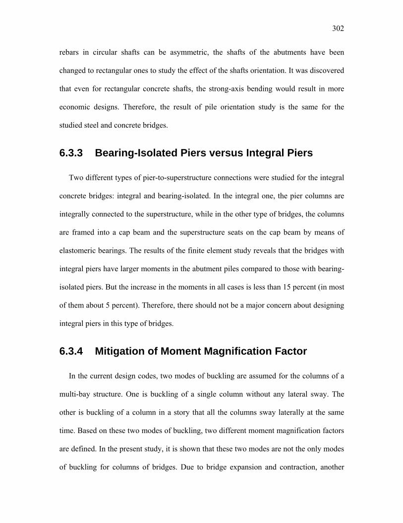
302
rebars in circular shafts can be asymmetric, the shafts of the abutments have been
changed to rectangular ones to study the effect of the shafts orientation. It was discovered
that even for rectangular concrete shafts, the strong-axis bending would result in more
economic designs. Therefore, the result of pile orientation study is the same for the
studied steel and concrete bridges.
6.3.3 Bearing-Isolated Piers versus Integral Piers
Two different types of pier-to-superstructure connections were studied for the integral
concrete bridges: integral and bearing-isolated. In the integral one, the pier columns are
integrally connected to the superstructure, while in the other type of bridges, the columns
are framed into a cap beam and the superstructure seats on the cap beam by means of
elastomeric bearings. The results of the finite element study reveals that the bridges with
integral piers have larger moments in the abutment piles compared to those with bearing-
isolated piers. But the increase in the moments in all cases is less than 15 percent (in most
of them about 5 percent). Therefore, there should not be a major concern about designing
integral piers in this type of bridges.
6.3.4 Mitigation of Moment Magnification Factor
In the current design codes, two modes of buckling are assumed for the columns of a
multi-bay structure. One is buckling of a single column without any lateral sway. The
other is buckling of a column in a story that all the columns sway laterally at the same
time. Based on these two modes of buckling, two different moment magnification factors
are defined. In the present study, it is shown that these two modes are not the only modes
of buckling for columns of bridges. Due to bridge expansion and contraction, another

303
mode of buckling can happen that is much more critical that the other two. In this mode,
the relative lateral translation of the column ends happen due to changes of the bridge
length while the moments are magnified by vertical loads, such as live load. It is shown
that this phenomenon is more critical in the case of jointed bridges. In integral abutment
bridges, at least one the abutments is helping the loaded column to mitigate its moment
magnification. The moment magnification factor for the new mode of buckling is also
recommended.
6.4 Recommendations for Future Research
In this dissertation, the behavior and responses of curved integral abutment bridges
were studied. The effects of several parameters were considered. But, there is still a need
to continue the research on this topic and develop a comprehensive design guide for this
type of bridges. One of the main problems that should be continued is to study the bridge
movement in other types of integral bridges. In this dissertation, a method for finding the
displacements of curved steel bridges was proposed. The displacements of other types of
bridges such as prestressed concrete girder bridges should also be studied. The effect of
different span length and number of spans should be investigated as well. The other
problem is to continue the study on pile orientation for other types of bridges and other
span lengths or ratios.
As some curved bridges are skewed at the ends, skewness is another topic that should
be incorporated into the effects of curvature. In the case of skew bridges, in several
previous reports, the only limitation that is set on the bridge geometry is a skew angle
less than 20 degrees. But, what is forgotten is that the skew angle is not the only factor

304
causing the rotation of the bridge. The other factor is the length-to-width ratio. When a
bridge has large length-to-width ratios, a small skew angle can cause a huge rotation in
the bridge structure. While for small ratios, the bridge may be able to tolerate larger skew
angles.

305
References
Al-Omaishi, N., Tadros, M. K., & Seguirant, S. J. (2009). Elasticity modulus, shrinkage,
and creep of high-strength concrete as adopted by AASHTO. PCI Journal, 54(3),
44-63.
American Association of State Highway and Transportation Officials. (1980). Guide
specifications for horizontally curved highway bridges - 1980. Washington, D.C:
A.A.S.H.T.O.
American Association of State Highway and Transportation Officials. (1993). Guide
specifications for horizontally curved highway bridges. Washington, D.C: American
Association of State Highway and Transportation Officials.
American Association of State Highway and Transportation Officials. (2007). AASHTO
LRFD bridge design specifications, customary U.S. units (4th ed.). Washington, DC:
American Association of State Highway and Transportation Officials.
American Association of State Highway and Transportation Officials. (2010). AASHTO
LRFD bridge design specifications (5th ed.). Washington, D.C: American
Association of State Highway and Transportation Officials.

306
American Association of State Highway and Transportation Officials. Subcommittee on
Bridges and Structures. (2003). AASHTO guide specifications for horizontally
curved steel girder highway bridges, 2003 : With design examples for I-girder and
box-girder bridges. Washington, DC: American Association of State Highway and
Transportation Officials.
American Institute of Steel Construction, American Institute of Steel Construction, &
Manual of steel construction. (2005). Steel construction manual. uniform title: Steel
construction (13th ed.). Chicago, Ill.: American Institute of Steel Construction.
American Iron and Steel Institute, Tennessee, Dept. of Transportation, Structures
Division, & National Steel Bridge Alliance. (1996). Integral abutments for steel
bridges. vol. 2, chapter 5, highway structures design handbook Printed by National
Steel Bridge Alliance.
American Petroleum Institute. (2005). Recommended practice for planning, designing,
and constructing fixed offshore platforms : Working stress design (21st ed.).
Washington, D.C: American Petroleum Institute.
Arockiasamy, M., & Sivakumar, M. (2005). Time-dependent behavior of continuous
composite integral abutment bridges. Practice Periodical on Structural Design and
Construction, 10(3), 161-170.
Arsoy, S., Barker, R. M., Duncan, J. M., Virginia Polytechnic and State University,
Charles E. Via Dept. of Civil and Environmental Engineering, Virginia
Transportation Research Council, et al. (1999). The behavior of integral abutment

307
bridges : Final contract report (FHWA/VTRC 00-CR3 ed.). Richmond, Va.:
Virginia Dept. of Transportation.
Barros, M. H. F. M., Martins, R. A. F., & Ferreira, C. C. (2001). Tension stiffening
model with increasing damage for reinforced concrete. Engineering Computations
(Swansea, Wales), 18(5-6), 759-785.
Bell, B. J., & Linzell, D. G. (2007). Erection procedure effects on deformations and
stresses in a large-radius, horizontally curved, I-girder bridge. Journal of Bridge
Engineering, 12(4), 467-476.
Boresi, A. P., & Schmidt, R. J. (2003). Advanced mechanics of materials (6th ed.). New
York: John Wiley & Sons.
Burke, M. P. (2009). Integral and semi-integral bridges. Chichester, U.K. ; Ames, Iowa:
Wiley-Blackwell.
Clough, G. W., Duncan, J. M., University of California, B., & Dept. of Civil Engineering.
(1971). Finite element analyses of retaining wall behavior. Berkeley, Calif: Dept. of
Civil Engineering, University of California.
Davidson, J. S., Keller, M. A., & Yoo, C. H. (1996). Cross-frame spacing and parametric
effects in horizontally curved I-girder bridges. Journal of Structural Engineering
New York, N.Y., 122(9), 1089-1096.
Davidson, J. S., & Yoo, C. H. (1996). Local buckling of curved I-girder flanges. Journal
of Structural Engineering New York, N.Y., 122(8), 936-947.

308
Davidson, J. S. (1996). Nominal bending and shear strength of horizontally curved steel
I-girder bridges
DeSantiago, E., Mohammadi, J., & Albaijat, H. M. O. (2005). Analysis of horizontally
curved bridges using simple finite-element models. Practice Periodical on
Structural Design and Construction, 10(1), 18-21.
Fennema, J. L., Laman, J. A., & Linzell, D. G. (2005). Predicted and measured response
of an integral abutment bridge. Journal of Bridge Engineering, (6)
Fiechtl, A. L. (1987). Approximate analysis of horizontally curved girder bridges. Austin,
TX: Center for Transportation Research , University of Texas at Austin.
Hall, D. H., Grubb, M. A., Yoo, C. H., United States, Federal Highway Administration,
National Cooperative Highway Research Program, et al. (1999). Improved design
specifications for horizontally curved steel girder highway bridges. Washington,
D.C: National Academy Press.
Hall, D. H., National Research Council (U.S.), Transportation Research Board, National
Cooperative Highway Research Program, & Bridge Software Development
International, Ltd. (1998). Recommended specifications for steel curved-girder
bridges. Coopersburg, PA: Bridge Software Development International.
Huo, X. S., Al-Omaishi, N., & Tadros, M. K. (2001). Creep, shrinkage, and modulus of
elasticity of high-performance concrete. ACI Materials Journal, 98(6), 440-449.

309
Kalayci, E. (2010). Analysis of curved integral abutment bridges, Master of Science
Thesis, University of Massachusetts Amherst,
http://scholarworks.umass.edu/theses/389/
Kulicki, J. M., National Cooperative Highway Research Program., American Association
of State Highway and Transportation Officials., & United States. Federal Highway
Administration. (2006). Development of LRFD specifications for horizontally curved
steel girder bridges. Washington, D.C.: Transportation Research Board.
Kulicki, J. M., National Cooperative Highway Research Program, & Modjeski and
Masters. (2005a). AASHTO-LRFD design example : Horizontally curved steel box
girder bridge. Harrisburg, Pa: Modjeski and Masters, Inc.
Kulicki, J. M., National Cooperative Highway Research Program, & Modjeski and
Masters. (2005b). AASHTO-LRFD design example: Horizontally curved steel I-
girder bridge. Harrisburg, Pa: Modjeski and Masters, Inc.
Linzell, D., Hall, D., & White, D. (2004). Historical perspective on horizontally curved I
girder bridge design in the united states. Journal of Bridge Engineering, 9(3), 218-
229.
Linzell, D., Leon, R. T., & Zureick, A. H. (2004). Experimental and analytical studies of
a horizontally curved steel I-girder bridge during erection. Journal of Bridge
Engineering, 9(6), 521-530.

310
Nevling, D., Linzell, D., & Laman, J. (2006). Examination of level of analysis accuracy
for curved I-girder bridges through comparisons to field data. Journal of Bridge
Engineering, 11(2), 160-168.
Ozbolt, J., & Bazant, Z. (1996). Numerical smeared fracture analysis: Nonlocal
microcrack interaction approach. International Journal for Numerical Methods in
Engineering, 39(4), [d]635-661.
Pugasap, K., Kim, W., & Laman, J. A. (2009). Long-term response prediction of integral
abutment bridges. Journal of Bridge Engineering, 14(2), 129-139.
Tadros, M. K., National Research Council (É.-U.), Transportation Research Board,
National Cooperative Highway Research Program, États-Unis, & Federal Highway
Administration. (2003). Prestress losses in pretensioned high-strength concrete
bridge girders. Washington, D.C: Transportation Research Board.
Tamboli, A. R. (2010). Handbook of structural steel connection design and details (2nd
ed.). New York: McGraw-Hill.
Thanasattayawibul, N. (2006). Curved Integral Abutment Bridges. Doctor of Philosophy
Dissertation, University of Maryland, College Park.
United States, Environmental Data Service, & National Climatic Center. (1900s).
Climatography of the united states. [Climatography of the United States Preceding
Title: Climatography of the United States]

311
Visher, S. S. (1954). Climatic atlas of the united states Cambridge, Harvard University
Press.
Wang, C., Salmon, C. G., & Pincheira, J. A. (2007). Reinforced concrete design (7th ed.).
Hoboken, NJ: John Wiley & Sons.
White, D. Development of design equation for curved steel I girder. (2001)
http://hdl.handle.net/1853/19352; Materials specified: Item Resolution URL
Instruction: Put this Resolution URL in a web browser to view this item.
Yakel, A. J. (2009). Flexural strength and ductility of high performance steel girders.
PhD Dissertation, University of Nebraska-Lincoln
Zureick, A., & Naqib, R. (1999). Horizontally curved steel I-girders state-of-the-art
analysis methods. Journal of Bridge Engineering, 4(1), 38-47.
Zureick, A., Naquib, R., Yadlosky, J. M., United States, Federal Highway
Administration, & HDR Engineering. (1994). Curved steel bridge research project.
interim report I, synthesis (FHWA-RD-93-129 ed.). McLean, Va; Springfield, Va:
Federal Highway Administration; Available through the National Technical
Information Service.
Maruri, R., & Petro, S. (2005). Integral Abutments and Jointless Bridges (IAJB) 2004
Survey Summary. The 2005 FHWA Conference (Integral Abutments and Jointless
Bridges). Baltimore, Maryland.
Akiyama, H. (2008). Fundamentally Structural Characteristics of Integral Bridges.

312
Kanazawa University, Graduate School of Natural Science & Technology.
American Association of State Highway and Transportation Officials. (2004). A Policy
on Geometric Design of Highways and Streets, 5th Edition. American Association of
State Highway and Transportation Officials, 2004.
Barker, R. M., Duncan, J. M., Rojiani, K. B., Ooi, P. S., Tan, C. K., & Kim, S. G. (1991).
National Cooperative Highway Research Program (NCHRP) Manuals for the Design of
Bridge Foundations. Washington: Transportation Research Board.
Bogard, D., & Matlock, H. (1980). Simplified Calculation of p-y Curves for Laterally
Loaded Piles. Unpublished Report, Ertec Inc.
Bonczar, C., Civjan, S., Brena, S., & DeJong, J. (2005). Behavior of Integral Abutment
Bridges: Field Data and Computer Modeling. Boston: EOT Office of Transportation
Planning.
Brena, S. F., Bonczar, C. H., Civjan, S. A., DeJong, J. T., & Crovo, D. S. (2007).
Evaluation of seasonal and Yearly Behavior of an Integral Abutment Bridge. Journal of
Bridge Engineering, 12 (3), 296-305.
Chavel, B. W., & Earls, C. J. (2006). Construction of a Horizontally Curved Steel I-
Girder Bridges. Part I: Erection Sequence. Journal of Bridge Engineering, 11 (1), 81-90.
Collin, P., Veljkovic, M., & Petursson, H. (2006). International Workshop on the Bridges
with Integral Abutments. Lulea University of Technology.
Galambos, T. V., Hajjar, J. F., Huang, W.-H., Pulver, B. E., Leon, R. T., & Rudie, B. J.
(2000). Comparison of measured and computed stresses in a steel curved girder bridge.
Journal of Bridge Engineering, 5 (3), 191-199.

313
Greimann, L. F., Wolde-Tinsae, Amde, A. M., & Yang, P. S. (1985). Effects of
Predrilling and Layered Soils on Piles. Journal of Geotechnical Engineering,111(1),18-31
Greimann, L. F., Wolde-Tinsae, Amde, A. M., & Yang, P. S. (1986). Nonlinear Analysis
of Integral Abutment Bridges. Journal of Structural Engineering, 112 (10), 2263-2280.
Howell, T. D., & Earls, C. J. (2007). Curved Steel I-Girder Bridge Response during
Construction Loading: Effects of Web Plumbness. Journal of Bridge Engineering, 12 (4),
485-493.
Iles, D. (2006). Integral Bridges in UK. International Workshop on IAB’s – Lulea
University of Technology.
Jayakumaran, S., Bergmann, M., Ashraf, S., & Norrish, C. (2005). Case Study: A
Jointless Structure to Replace the Belt Parkway Bridge Over Ocean Parkway”,. FHWA
Conference.
Kim, W. S., Laman, J. L., & Linzell, D. G. (2007). Live Load Radial Moment
Distribution for Horizontally Curved Bridges. Journal of Bridge Engineering, 12 (6), 727-
736.
Linzell, D. G. (1999). Studies of a full-scale horizontally curved steel I-girder bridge
system under self-weight. PhD Dissertation, Georgia Institute of Technology, School of
Civil and Environmental Engineering.
McElwain, B. A., & Laman, J. A. (2000). Experimental Verification of Horizontally
Curved I-Girder Bridge Behavior. Journal of Bridge Engineering, 5 (4), 284-292.
Ministry of Transportation - Province of Ontario. (1999). Performance of Integral
Abutment Bridges.

314
Moorty, S., & Roeder, C. W. (1992). Temperature-Dependent Bridge Movements.
Journal of Structural Engineering , 118 (4), 1090-1105.
Roeder, C. W., & Moorty, S. (1990). Thermal Movements in Bridges. Transportation
Research Record , 1290 , 135-143. Washington, D.C.: Transportation Research Board,
National research Council.
Samaan, M., Sennah, K., & Kennedy, J. B. (2002). Positioning of bearings for curved
continuous spread-box girder bridges. Canadian Journal of Civil Engineering , 29 (5),
641-652. 179
Ting, J. M., & Faraji, S. (1998). Streamlined Analysis and Design of Integral Abutment
Bridges. University of Massachusetts Lowell, Department of Civil and Environmental
Engineering. Amherst: University of Massachusetts Transportation Center.
Womack, K., Halling, M., & Bott, S. (2001). Static and dynamic testing of a curved steel
girder bridge in Salt Lake City, Utah. Utah Department of Transportation.
Zhang, H., Huang, D., & Wang, T.-L. (2005). Lateral load distribution in curved steel I-
girder bridges. Journal of Bridge Engineering, 10 (3), 281-290.
VTrans. 2009. Integral Abutment Bridge Design Guidelines. Montpelier, Vermont :
VTrans, 2009.
ABAQUS Analysis User’s Manual, version 6.9-1 (2006), Hibbit, Karlsson & Sorenson,
Inc., Pawtucket, Rhode Island. ABAQUS Theory Manual, version 6.6-1 (2006), Hibbit,
Karlsson & Sorenson, Inc., Pawtucket, Rhode Island.
Carreira D. J., & Chu K. (1985). Stress-Strain Relationship for Plain Concrete in
Compression. ACI Journal, November-December 1985, 797-804.

315
National Steel Bridge Alliance, American Iron and Steel Institute. 1996. Integral
Abutments for Steel Bridges. s.l.: Tennessee Department of Transportation, 1996.
White, D. W., Zureick, A. H., Phoawanich, N., and Jung, S. (2001). "Development of
Unified Equations for Design of Curved and Straight Steel Bridge I Girders," Final
Report, Prepared for American Iron and Steel Institute Transportation and Infrastructure
Committee, Professional Service Industries, Inc., and Federal Highway Administration,
School of Civil and Environmental Engineering, Georgia Institute of Technology,
Atlanta, GA.
White, D. W. (2008). "Unified Flexural Resistance Equations for Stability Design of
Steel I-Section Members: Overview." Journal of Structural Engineering, 134(9), ASCE,
1405-1424.
White, D. W., and Barker, M. G. (2008). "Shear Resistance of Transversely Stiffened
Steel I-Girders." Journal of Structural Engineering, 134(9), ASCE, 1425-1436.
White, D. W., Barker, M. G., and Azizinamini, A. (2008). "Shear Strength and Moment-
Shear Interaction in Transversely Stiffened Steel I-Girders." Journal of Structural
Engineering, 134(9), ASCE, 1437-1449.
White, D. W., and Duk Kim, Y. (2008). "Unified Flexural Resistance Equations for
Stability Design of Steel I-Section Members: Moment Gradient Tests." Journal of
Structural Engineering, 134(9), ASCE, 1471-1486. 226
White, D. W., and Jung, S. (2008). "Unified Flexural Resistance Equations for Stability
Design of Steel I-Section Members: Uniform Bending Tests." Journal of Structural
Engineering, 134(9), ASCE, 1450-1470.

316
Marchon, P. H. A. (2007). Nonlinear Finite Element Analysis of Composite Bridges At
Ultimate Load, Master of Science Thesis, University of Nebraska-Lincoln

317
Appendix A
Effect of Bridge Length and
Curvature on Shear Force of
Abutment Piles
In Appendix 1, the developed shear force in the abutment piles of the studied steel
integral bridges is investigated in more details. First, the shear force of piles due to each
load or load effect is plotted and discussed. Then, the envelope of the shear forces in
different load combinations which is a design parameter is studied. Similar to the section
4.4.1A), the loads are presented based on their normalized weight factor.
A1 Contraction
Figure A-1. shows the abutment piles shear forces under contraction loading for
different bridge length and radii of curvature. One can see that the shear forces decrease
as the radius of curvature decreases. The other observation is that in a straight bridge the
shear force increases as the bridge gets longer. But in a curved bridge when the length
increases the shear forces increases up to a certain length and after that it starts to reduce.

318
Figure A-1. Maximum Shear Force in Abutment Piles Due to Contraction
The piles shear forces are normalized in Figure A-2. by dividing the shear force of the
curved bridges by that of the straight bridge of the same length. It can be seen that the
shear forces of curved bridges can reduce about 75 percent when the bridge has a small
radius of curvature.
0
10
20
30
40
50
60
70
80
90
300 400 500 600 700 800 900
Shear Force (kip)
Bridge Length (ft)
Integral Abutment ‐ Piers Bearing Type: Elastomeric
R=infinity
R=1000'
R=538'
R=300'
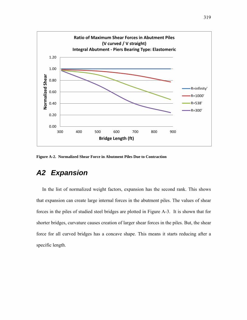
319
Figure A-2. Normalized Shear Force in Abutment Piles Due to Contraction
A2 Expansion
In the list of normalized weight factors, expansion has the second rank. This shows
that expansion can create large internal forces in the abutment piles. The values of shear
forces in the piles of studied steel bridges are plotted in Figure A-3. It is shown that for
shorter bridges, curvature causes creation of larger shear forces in the piles. But, the shear
force for all curved bridges has a concave shape. This means it starts reducing after a
specific length.
0.00
0.20
0.40
0.60
0.80
1.00
1.20
300 400 500 600 700 800 900
Normalized
She
ar
Bridge Length (ft)
Ratio of Maximum Shear Forces in Abutment Piles(V curved / V straight)
Integral Abutment ‐ Piers Bearing Type: Elastomeric
R=infinity'
R=1000'
R=538'
R=300'

320
Figure A-3. Maximum Shear Force in Abutment Piles Due to Expansion
The shear forces are Normalized in Figure A-4. This picture shows that the shear
force of piles of curved bridges are about two times of that of equivalent straight bridges.
But for highly curved bridges it can be half of the shear force of straight bridge for long
bridges of length about 900 feet.
0
5
10
15
20
25
30
35
300 400 500 600 700 800 900
Shear Force (kip)
Bridge Length (ft)
Integral Abutment ‐ Piers Bearing Type: Elastomeric
R=infinity
R=1000'
R=538'
R=300'
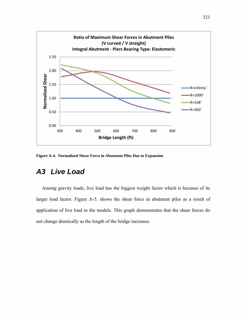
321
Figure A-4. Normalized Shear Force in Abutment Piles Due to Expansion
A3 Live Load
Among gravity loads, live load has the biggest weight factor which is because of its
larger load factor. Figure A-5. shows the shear force in abutment piles as a result of
application of live load to the models. This graph demonstrates that the shear forces do
not change drastically as the length of the bridge increases.
0.00
0.50
1.00
1.50
2.00
2.50
300 400 500 600 700 800 900
Normalized
She
ar
Bridge Length (ft)
Ratio of Maximum Shear Forces in Abutment Piles(V curved / V straight)
Integral Abutment ‐ Piers Bearing Type: Elastomeric
R=infinity'
R=1000'
R=538'
R=300'
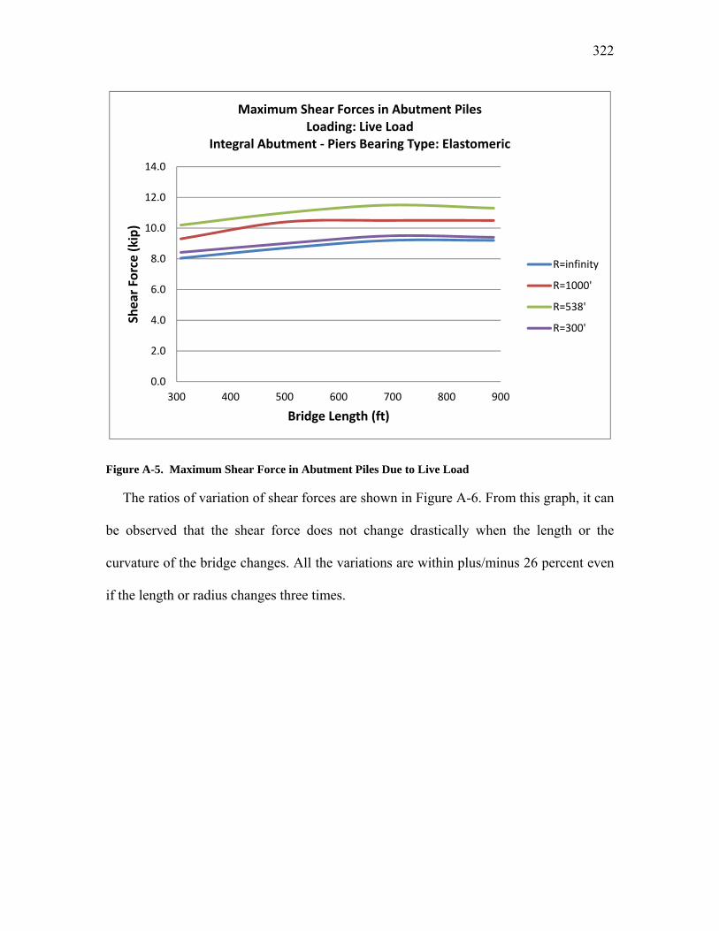
322
Figure A-5. Maximum Shear Force in Abutment Piles Due to Live Load
The ratios of variation of shear forces are shown in Figure A-6. From this graph, it can
be observed that the shear force does not change drastically when the length or the
curvature of the bridge changes. All the variations are within plus/minus 26 percent even
if the length or radius changes three times.
0.0
2.0
4.0
6.0
8.0
10.0
12.0
14.0
300 400 500 600 700 800 900
Shear Force (kip)
Bridge Length (ft)
Maximum Shear Forces in Abutment PilesLoading: Live Load
Integral Abutment ‐ Piers Bearing Type: Elastomeric
R=infinity
R=1000'
R=538'
R=300'

323
Figure A-6. Normalized Shear Force in Abutment Piles Due to Live Load
A4 Wind Load
The shear forces of the abutment piles are given in Figure A-7. This plot shows that up
to a length of about 600 feet, the shear forces in bridges with different radius of curvature
are almost the same as that of the straight bridge of equal length. However, as the length
of the bridge goes beyond 600 feet, the effect of bridge curvature is more profound and
larger differences are observed.
0.00
0.20
0.40
0.60
0.80
1.00
1.20
1.40
300 400 500 600 700 800 900
Normalized
She
ar
Bridge Length (ft)
Ratio of Maximum Shear Forces in Abutment Piles(V curved / V straight)Loading: Live Load
Integral Abutment ‐ Piers Bearing Type: Elastomeric
R=infinity'
R=1000'
R=538'
R=300'

324
Figure A-7. Maximum Shear Force in Abutment Piles Due to Wind Load
Figure A-8. discusses the ratios of the shear forces due to wind load. It is seen that for
a bridge of about 900 feet length, the shear force in a curved bridge can be about 50
percent larger than that of a straight bridge.
0.00
2.00
4.00
6.00
8.00
10.00
12.00
14.00
16.00
18.00
20.00
300 400 500 600 700 800 900
Shear Force (kip)
Bridge Length (ft)
Integral Abutment ‐ Piers Bearing Type: Elastomeric
R=infinity
R=1000'
R=538'
R=300'

325
Figure A-8. Normalized Shear Force in Abutment Piles Due to Wind Load
A5 Dead Load
The shear response of the piles of integral steel bridges subjected to dead load is
depicted in Figure A-9. Like live load, deal load has a decreasing trend as the length of
the bridge increases. The other remark is that, although the straight bridge shows lower
shear force for shorter bridges, as the length increases the curves of non-straight bridges
fall below that of straight ones.
0.00
0.20
0.40
0.60
0.80
1.00
1.20
1.40
1.60
1.80
300 400 500 600 700 800 900
Normalized
She
ar
Bridge Length (ft)
Ratio of Maximum Shear Forces in Abutment Piles(V curved / V straight)
Integral Abutment ‐ Piers Bearing Type: Elastomeric
R=infinity'
R=1000'
R=538'
R=300'

326
Figure A-9. Maximum Shear Force in Abutment Piles Due to Dead Load
Figure A-10. illustrates the normalized shear force of the abutment piles. It shows that
the greatest drop in shear force per length increment is for the highest curvature, i.e.
R=300 feet. When the bridge has lower curvature, the response is closer to that of straight
bridge, which seems reasonable.
0
2
4
6
8
10
12
14
300 400 500 600 700 800 900
Shear Force (kip)
Bridge Length (ft)
Integral Abutment ‐ Piers Bearing Type: Elastomeric
R=infinity
R=1000'
R=538'
R=300'

327
Figure A-10. Normalized Shear Force in Abutment Piles Due to Dead Load
A6 Concrete Shrinkage
Figure A-11. shows the shear force of piles when the bridge is subject to the effects of
concrete shrinkage. The response of straight bridges and curved bridges with large radius
is a convex curve, while that of highly curved bridges is concave. As such, shear forces
increase for larger radii of curvature (including infinity) and finally decrease for smaller
radii (after the maximum point). The other point is that the shear force of curved bridges
longer than about 700 feet is less than the force of a straight bridge of the same length.
0.00
0.20
0.40
0.60
0.80
1.00
1.20
1.40
1.60
300 400 500 600 700 800 900
Normalized
She
ar
Bridge Length (ft)
Ratio of Maximum Shear Forces in Abutment Piles(V curved / V straight)
Integral Abutment ‐ Piers Bearing Type: Elastomeric
R=infinity'
R=1000'
R=538'
R=300'

328
Figure A-11. Maximum Shear Force in Abutment Piles Due to Concrete Shrinkage
Normalized shear forces of the abutment piles are plotted versus length in Figure A-
12. This picture shows the shear force from another perspective. In shorter bridges, the
shear forces of piles of highly curve bridges due to shrinkage are about two times larger
than that of straight bridges. As the length goes up to about 900 feet, the shear force
drops down to about 60 percent of the shear of the equivalent straight bridge. Also, a
pivot point with approximate length of 700 feet is observable.
0
5
10
15
20
25
30
300 400 500 600 700 800 900
Shear Force (kip)
Bridge Length (ft)
Integral Abutment ‐ Piers Bearing Type: Elastomeric
R=infinity
R=1000'
R=538'
R=300'

329
Figure A-12. Normalized Shear Force in Abutment Piles Due to Concrete Shrinkage
A7 Horizontal Earth Pressure
Figure A-13. shows the shear forces of the abutment piles when horizontal earth
pressure is applied to the bridge. The shear force in straight bridges does not depend on
the length of the bridge which is reasonable. But, in the case of curved bridges, it changes
as the length changes. For small radii of curvature like 300 feet, it has the largest values
which tend to be constant for longer bridges. For larger radii like 1000 feet, it shows
increasing trend as the length increases.
0.00
0.50
1.00
1.50
2.00
2.50
300 400 500 600 700 800 900
Normalized
She
ar
Bridge Length (ft)
Ratio of Maximum Shear Forces in Abutment Piles(V curved / V straight)
Integral Abutment ‐ Piers Bearing Type: Elastomeric
R=infinity'
R=1000'
R=538'
R=300'
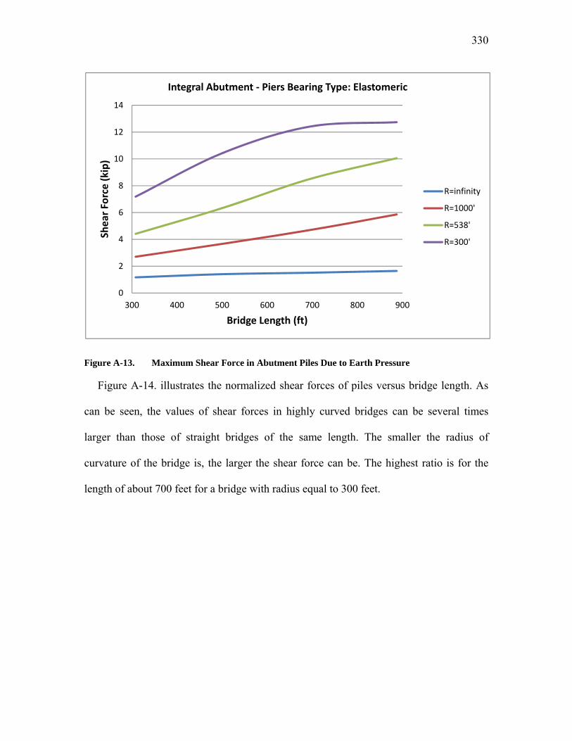
330
Figure A-13. Maximum Shear Force in Abutment Piles Due to Earth Pressure
Figure A-14. illustrates the normalized shear forces of piles versus bridge length. As
can be seen, the values of shear forces in highly curved bridges can be several times
larger than those of straight bridges of the same length. The smaller the radius of
curvature of the bridge is, the larger the shear force can be. The highest ratio is for the
length of about 700 feet for a bridge with radius equal to 300 feet.
0
2
4
6
8
10
12
14
300 400 500 600 700 800 900
Shear Force (kip)
Bridge Length (ft)
Integral Abutment ‐ Piers Bearing Type: Elastomeric
R=infinity
R=1000'
R=538'
R=300'

331
Figure A-14. Normalized Shear Force in Abutment Piles Due to Earth Pressure
A8 Centrifugal Force
The shear forces of piles created by centrifugal force of the live load are plotted versus
length in Figure A-15. As can be observed, the piles shear force is approximately
unchanged upon variation of bridge length or radius. As there is no centrifugal force in
straight bridges, a normalized shear force is not defined for this load in the same way as
the other loads.
0.00
1.00
2.00
3.00
4.00
5.00
6.00
7.00
8.00
9.00
300 400 500 600 700 800 900
Normalized
She
ar
Bridge Length (ft)
Ratio of Maximum Shear Forces in Abutment Piles(V curved / V straight)
Integral Abutment ‐ Piers Bearing Type: Elastomeric
R=infinity'
R=1000'
R=538'
R=300'

332
Figure A-15. Maximum Shear Force in Abutment Piles Due to Centrifugal Force
A9 Weight of Wearing Surface
Figure A-16. represents the shear force of abutment piles for different bridge length
and curvature. As can be seen, the general trend is similar to the other gravity loads. The
shear force reduces as the length of the bridge increases and the slope of reduction is
larger for smaller radii of curvature. As expected, the shear force for straight bridges is
almost the same for different bridge lengths. This is attributed to the fact that this shear
force in a straight bridge is mainly a function of the end span length which has been the
same for all studied bridge.
0.0
0.5
1.0
1.5
2.0
2.5
3.0
3.5
4.0
4.5
300 400 500 600 700 800 900
Shear Force (kip)
Bridge Length (ft)
Integral Abutment ‐ Piers Bearing Type: Elastomeric
R=infinity
R=1000'
R=538'
R=300'

333
Figure A-16. Maximum Shear Force in Abutment Piles Due to Weight of Wearing Surface
By dividing the shear force of the curved bridges by that of the straight bridge of the
same length, the shear forces are normalized which are graphed in Figure A-17. As one
can observe, the normalized shear graph is very similar to that of dead load. This is
because these two loadings are of the same nature. Again, it is seen that the rate of
changes is maximum for smallest radius of curvature.
0.0
0.5
1.0
1.5
2.0
2.5
300 400 500 600 700 800 900
Shear Force (kip)
Bridge Length (ft)
Integral Abutment ‐ Piers Bearing Type: Elastomeric
R=infinity
R=1000'
R=538'
R=300'

334
Figure A-17. Normalized Shear Force in Abutment Piles Due to Weight of Wearing Surface
A10 Braking Force
The shear force caused by braking load of the live loads is illustrated in Figure A-18.
Braking force has one of the smallest weight factors among various loads. That can be
ascertained by looking the shear values developed in the piles by this loading. The shear
forces are tiny. The change in the rate of forces which starts for lengths larger than 450
feet, is because of the change in definition of the load in that range of lengths. The
normalized shear forces are also shown in Figure A-19.
0.00
0.20
0.40
0.60
0.80
1.00
1.20
1.40
1.60
300 400 500 600 700 800 900
Normalized
She
ar
Bridge Length (ft)
Ratio of Maximum Shear Forces in Abutment Piles(V curved / V straight)
Integral Abutment ‐ Piers Bearing Type: Elastomeric
R=infinity'
R=1000'
R=538'
R=300'

335
Figure A-18. Maximum Shear Force in Abutment Piles Due to Braking Force
Figure A-19. Normalized Shear Force in Abutment Piles Due to Braking Force
0
1
1
2
2
3
3
300 400 500 600 700 800 900
Shear Force (kip)
Bridge Length (ft)
Integral Abutment ‐ Piers Bearing Type: Elastomeric
R=infinity
R=1000'
R=538'
R=300'
0.00
0.50
1.00
1.50
2.00
2.50
3.00
3.50
4.00
4.50
300 400 500 600 700 800 900
Normalized
She
ar
Bridge Length (ft)
Ratio of Maximum Shear Forces in Abutment Piles(V curved / V straight)
Integral Abutment ‐ Piers Bearing Type: Elastomeric
R=infinity'
R=1000'
R=538'
R=300'
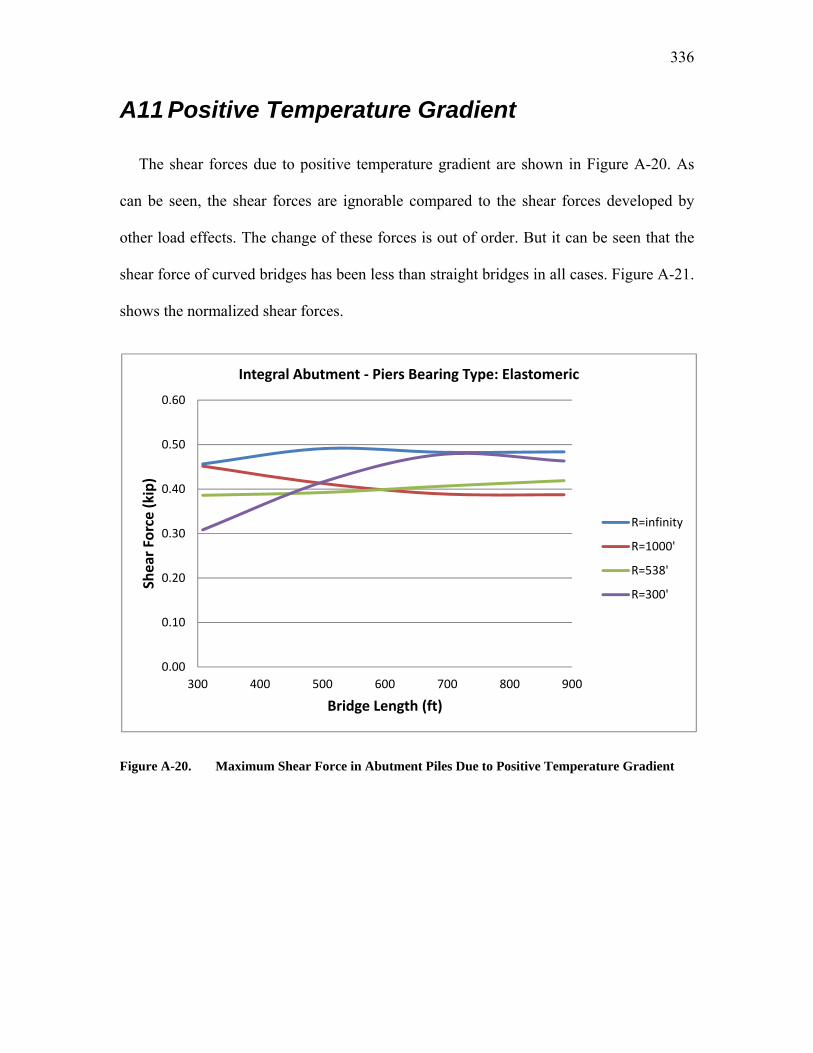
336
A11 Positive Temperature Gradient
The shear forces due to positive temperature gradient are shown in Figure A-20. As
can be seen, the shear forces are ignorable compared to the shear forces developed by
other load effects. The change of these forces is out of order. But it can be seen that the
shear force of curved bridges has been less than straight bridges in all cases. Figure A-21.
shows the normalized shear forces.
Figure A-20. Maximum Shear Force in Abutment Piles Due to Positive Temperature Gradient
0.00
0.10
0.20
0.30
0.40
0.50
0.60
300 400 500 600 700 800 900
Shear Force (kip)
Bridge Length (ft)
Integral Abutment ‐ Piers Bearing Type: Elastomeric
R=infinity
R=1000'
R=538'
R=300'

337
Figure A-21. Normalized Shear Force in Abutment Piles Due to Positive Temperature Gradient
A12 Negative Temperature Gradient
Having the smallest weight factor among all loads proves trifling nature of negative
temperature gradient in design procedure of studied bridges. The shear forces are all less
than 0.2 kips. Therefore, the regime of their changes is not discussed. The normalized
shear force is shown in Figure A-23. It shows that this tiny shear force in curved bridges
can be in some conditions smaller and in some other cases greater than that of straight
counterpart which is not of great importance.
0.00
0.20
0.40
0.60
0.80
1.00
1.20
300 400 500 600 700 800 900
Normalized
She
ar
Bridge Length (ft)
Ratio of Maximum Shear Forces in Abutment Piles(V curved / V straight)
Integral Abutment ‐ Piers Bearing Type: Elastomeric
R=infinity'
R=1000'
R=538'
R=300'

338
Figure A-22. Maximum Shear Force in Abutment Piles Due to Negative Temperature Gradient
0.00
0.02
0.04
0.06
0.08
0.10
0.12
0.14
0.16
300 400 500 600 700 800 900
Shear Force (kip)
Bridge Length (ft)
Integral Abutment ‐ Piers Bearing Type: Elastomeric
R=infinity
R=1000'
R=538'
R=300'

339
Figure A-23. Normalized Shear Force in Abutment Piles Due to Negative Temperature Gradient
A13 Combination of the Loads
After discussing the effect of bridge length and curvature on the shear force of
abutment piles of studied bridges, in this section the envelope of shear force in different
load combinations of AASHTO code is studied in more details. As can be observed from
Figure A-24. the shear forces of piles in straight bridges increase as the length of the
bridge increases. But, in curved bridge variations is a function of curvature. In bridges
with large radius of curvature, the trend is somehow similar to straight bridges, but with a
more moderate rate of change. In highly curved bridge, the slope of changes reduces so
that the shear forces can decrease as the length increases.
0.00
0.20
0.40
0.60
0.80
1.00
1.20
300 400 500 600 700 800 900
Normalized
She
ar
Bridge Length (ft)
Ratio of Maximum Shear Forces in Abutment Piles(V curved / V straight)
Integral Abutment ‐ Piers Bearing Type: Elastomeric
R=infinity'
R=1000'
R=538'
R=300'

340
Figure A-24. Envelope of Maximum Shear Force in Abutment Piles in Different Load
Combinations
Figure A-25. shows the normalized factored shear force envelope in the abutment
piles. it can be observed that the design shear force in a curved bridge of small length
(L=300’) is larger than that of the equivalent straight bridge. It also shows that depending
on the bridge curvature, the shear force of curved bridge is equal to that of the straight.
For bridge longer than that specific length, the shear force starts to be smaller than that of
the straight bridge so that at the length of about 900 feet, the shear force of the pile can be
as small as 45 percent of the shear force of straight bridge. This shows that piles of long
curved bridge are more designable compared to straight bridge with equal length from
shear design point of view.
0
20
40
60
80
100
120
140
300 400 500 600 700 800 900
Shear Force (kip)
Bridge Length (ft)
Integral Abutment ‐ Piers Bearing Type: Elastomeric
R=infinity
R=1000'
R=538'
R=300'

341
Figure A-25. Envelope of Normalized Shear Force in Abutment Piles in Different Load
Combinations
0.00
0.20
0.40
0.60
0.80
1.00
1.20
1.40
1.60
300 400 500 600 700 800 900
Normalized
She
ar
Bridge Length (ft)
Ratio of Maximum Shear Forces in Abutment Piles(V curved / V straight)
Integral Abutment ‐ Piers Bearing Type: Elastomeric
R=infinity'
R=1000'
R=538'
R=300'

342
Appendix B
MATLAB Moment-curvature
Program
In this appendix, the MATLAB program developed to analyze the moment capacity of
the composite steel section at the face of integral abutment is presented:
disp('Units: kips, inch');
format long;
disp('Is it the first time you are running the program (after loading MATLAB)?');
first=input('y for "yes" or n for "no" (Default= no): ','s');
if isempty(first)
first='n';
end
if first=='y'
B=zeros(100,1);
D=zeros(100,1);
material=zeros(100,1);
end
% color('green');
n_sec = input('Number of section changes? (Default=5)');
if isempty(n_sec)
n_sec = 5;

343
end
sum_D=zeros(n_sec,1);
for i=1:n_sec
disp('%%'); disp('%%'); disp(' Width B(i,1)was:');
disp(B(i,1));
disp('Press "Enter" if there is no changes in the section width.');
Btemp= input('Width of the section? ');
if isempty(Btemp)
aaaa=1;
else
B(i,1) = Btemp;
end
disp('%%'); disp('%%'); disp(' Depth(i,1)was:');
disp(D(i,1));
disp('Press "Enter" if there is no changes in the section depth.');
Dtemp= input('Depth of the section? ');
if isempty(Dtemp)
aaaa=1;
else
D(i,1) = Dtemp;
end
disp('%%'); disp('%%');
disp('Material of the section:');
disp(' Enter 1 for GR50 Steel');
disp(' 2 for GR60 Steel');
disp(' 3 for GR100 Steel');
disp(' 4 for NSC');
disp(' 5 for HSC');
disp(' 6 for UHPC');
% material(i,1)= input('Select a Material (1 to 6):');
disp(' Material(i,1)was:');

344
if material(i,1)== 1;
disp(' 1: GR50 Steel');
elseif material(i,1)==2;
disp(' 2: GR60 Steel');
elseif material(i,1)==3;
disp(' 3: GR100 Steel');
elseif material(i,1)==4;
disp(' 4: NSC');
elseif material(i,1)==5;
disp(' 5: HSC');
elseif material(i,1)==6;
disp(' 6: UHPC');
end
disp(material(i,1));
disp('Press "Enter" if there is no changes in the section material.');
mattemp= input('Material of the section? ');
if isempty(mattemp)
aaaa=1;
else
material(i,1) = mattemp;
end
end
% forming the total height
h=0;
for i=1:n_sec
h=h+D(i,1);
end
disp('%%'); disp('%%');
disp('Total Height=');
disp(h);
% forming the partial depths

345
sum_D(1,1)=D(1,1);
for i=2:n_sec
sum_D(i,1)=sum_D(i-1,1)+D(i,1);
end
disp('%%'); disp('%%');
n = input('Number of increments in the section (for Default n=1000 Press "Enter")?');
if isempty(n)
n = 1000;
end
% setting breadth and material for each increment
b=zeros(n+1,1);
d=zeros(n+1,1);
mat=zeros(n+1,1);
for j=1:n_sec-1
for i=1:n+1
d(i,1)=(i-1)/n*h;
if d(i,1)<=sum_D(1,1)
b(i,1)=B(1,1);
mat(i,1)=material(1,1);
elseif d(i,1)>sum_D(j,1)
b(i,1)=B(j+1,1);
mat(i,1)=material(j+1,1);
else
b(i,1)=b(i,1)+0;
end
end
end
% k represents the current location of N.A.
k=round(n/2);
% integer
% incofe is the increments of strain

346
incofe=0.00022;
% n_inc is the number of increments of strain to be considered (ie max strain)
n_e_inc=100;
strain=zeros(n+1,1);
stress=zeros(n+1,1);
f=zeros(n+1,1);
m=zeros(n+1,1);
curvature=zeros(n_e_inc+1,1);
M=zeros(n_e_inc+1,1);
M(1,1)=0;
curvature(1,1)=0;
%E=20;
%a=2;
%Fy=2;
%ey=Fy/E;
dy=h/n;
% an approximate method for calculating the convergence limit
dummy_force=zeros(n_sec,1);
for i=1:n_sec
if material(i,1)== 1;
ff=50;
elseif material(i,1)==2;
ff=60;
elseif material(i,1)==3;
ff=100;
elseif material(i,1)==4;
ff=4;
elseif material(i,1)==5;
ff=15;
elseif material(i,1)==6;
ff=18.4;

347
end
dummy_force(i,1)=B(i,1)*D(i,1)*ff;
end
dum_force=0.003*sum(dummy_force(:,1));
disp('%%'); disp('%%');
disp('3/1000 of yield axial force of the section is:');
disp(dum_force);
CL= input('Convergence Force Limit (for Default=0.003*Yield force Press "Enter")?');
NoConv=0;
if isempty(CL)
CL = dum_force;
end
disp('%%'); disp('%%');
disp('RUNNING ...');
pause(0.1);
rup_flag=0;
if NoConv==0
for j=2:n_e_inc+1
if (rup_flag==0 && NoConv==0)
etop=(j-1)*incofe;
for i=1:n+1
strain(i,1)=-etop+(i-1)/k*etop;
if mat(i,1)== 1;
StressGR50;
elseif mat(i,1)==2;
StressGR60;
elseif mat(i,1)==3;
StressGR100;
elseif mat(i,1)==4;
StressNSC;
elseif mat(i,1)==5;

348
StressHSC;
elseif mat(i,1)==6;
StressUHPC;
end
end
for i=1:n
f(i,1)=(stress(i,1)+stress(i+1,1))/2*(b(i,1)+b(i+1,1))/2*dy;
end
F=sum(f(:,1));
while (abs(F)>CL && NoConv==0)
if (F>0 && k<n-1)
k=k+1;
for i=1:n+1
strain(i,1)=-etop+(i-1)/k*etop;
if mat(i,1)== 1;
StressGR50;
elseif mat(i,1)==2;
StressGR60;
elseif mat(i,1)==3;
StressGR100;
elseif mat(i,1)==4;
StressNSC;
elseif mat(i,1)==5;
StressHSC;
elseif mat(i,1)==6;
StressUHPC;
end
end
for i=1:n
f(i,1)=(stress(i,1)+stress(i+1,1))/2*(b(i,1)+b(i+1,1))/2*dy;
end

349
elseif (F<0 && k>1)
k=k-1;
for i=1:n+1
strain(i,1)=-etop+(i-1)/k*etop;
if mat(i,1)== 1;
StressGR50;
elseif mat(i,1)==2;
StressGR60;
elseif mat(i,1)==3;
StressGR100;
elseif mat(i,1)==4;
StressNSC;
elseif mat(i,1)==5;
StressHSC;
elseif mat(i,1)==6;
StressUHPC;
end
end
for i=1:n
f(i,1)=(stress(i,1)+stress(i+1,1))/2*(b(i,1)+b(i+1,1))/2*dy;
end
else
NoConv=1;
disp('There is no convergence!');
end
F=sum(f(:,1));
end;
for i=1:n
m(i,1)=f(i,1)*(i-0.5)*dy;
end
M(j,1)=sum(m(:,1));

350
curvature(j,1)=etop/(k*dy);
for i=1:n+1
if rup_flag==0
if mat(i,1)== 1;
StrainGR50;
elseif mat(i,1)==2;
StrainGR60;
elseif mat(i,1)==3;
StrainGR100;
elseif mat(i,1)==4;
StrainNSC;
elseif mat(i,1)==5;
StrainHSC;
elseif mat(i,1)==6;
StrainUHPC;
end
end
end
elseif rup_flag==1
M(j,1)=M(j-1,1);
curvature(j,1)=curvature(j-1,1);
end
disp(curvature(j,1));
disp(M(j,1));
% plot(curvature(j,1),M(j,1));
end
else
disp('There is no convergence!');
end
disp('Total Height=');
disp(h);

351
disp('Maximum Curvarture=');
disp(curvature(j,1));
disp('Maximum Moment=');
disp(M(j,1));
disp('Top Strain=');
disp(strain(1,1));
disp('Bottom Strain=');
disp(strain(n+1,1));
plot(curvature,M);
% plot stress
z=zeros(n+1,1);
for i=1:n+1
z(i,1)=h-d(i,1);
end
plot(stress,z);