on learning with integral operatorsweb.mit.edu/lrosasco/www/publications/operator_estimates.pdfthe...
TRANSCRIPT
Journal of Machine Learning Research () Submitted 12/04; Published
On Learning with Integral Operators
Lorenzo Rosasco, [email protected] for Biological and Computational Learning, MIT,Cambridge, MA, USA& Dipartimento di Informatica e Scienze dell’Informazione,Universita di Genova, Italy
Mikhail Belkin, [email protected] of Computer Science and Engineering,Ohio State University, U.S.A.
Ernesto De Vito [email protected]
Dipartimento di Scienze per l’Architettura,Universita di Genova, Italy& INFN, Sezione di Genova, Italy
Editor:
Abstract
A large number of learning algorithms, for example, spectral clustering, kernel PrincipalComponents Analysis and many manifold methods are based on estimating eigenvaluesand eigenfunctions of operators defined by a similarity function or a kernel, given empiricaldata. Thus for the analysis of algorithms, it is an important problem to be able to assessthe quality of such approximations. The contribution of our paper is two-fold:1. We use a technique based on a concentration inequality for Hilbert spaces to providenew much simplified proofs for a number of results in spectral approximation.2. Using these methods we provide several new results for estimating spectral properties ofthe graph Laplacian operator extending and strengthening results from von Luxburg et al.(2008).Keywords: spectral convergence, empirical operators, learning integral operators, per-turbation methods
1. Introduction
A broad variety of methods for machine learning and data analysis from Principal Com-ponents Analysis (PCA) to Kernel PCA, Laplacian-based spectral clustering and manifoldmethods, rely on estimating eigenvalues and eigenvectors of certain data-dependent matri-ces. In many cases these matrices can be interpreted as empirical versions of underlyingintegral operators or closely related objects, such as continuous Laplacian operators. Thusestablishing connections between empirical operators and their continuous counterparts isessential to understanding these algorithms. In this paper, we propose a method for an-alyzing empirical operators based on concentration inequalities in Hilbert spaces. This
c© Lorenzo Rosasco, Mikhail Belkin Ernesto De Vito.
Rosasco, Belkin, De Vito
technique together with perturbation theory results allows us to derive a number of resultson spectral convergence in an exceptionally simple way. We note that the approach usingconcentration inequalities in a Hilbert space has already been proved useful for analyz-ing supervised kernel algorithms, see De Vito et al. (2005b), Yao et al. (2007), Bauer et al.(2007), Smale and Zhou (2005). Here we develop on this approach to provide a detailed andcomprehensive study of perturbation results for empirical estimates of integral operators aswell as empirical graph Laplacians.
In recent years several works started considering these connections. The first studyof this problem appeared in Koltchinskii and Gine (2000), Koltchinskii (1998), where theauthors consider integral operators defined by a kernel. In Koltchinskii and Gine (2000)the authors study the relation between the spectrum of an integral operator with respectto a probability distribution and its (modified) empirical counterpart in the frameworkof U -statistics. In particular they prove that the `2 distance between the two (ordered)spectra goes to zero under the assumption that the kernel is symmetric and square inte-grable. Moreover, under some stronger conditions, rates of convergence and distributionallimit theorems are obtained. The results are based on an inequality due to Lidskii andto Wielandt for finite dimensional matrices and the Marcinkiewicz law of large numbers.In Koltchinskii (1998) similar results were obtained for convergence of eigenfunctions and,using the triangle inequality, for spectral projections. These investigations were continuedin Mendelson and Pajor (2005, 2006), where it was shown that, under the assumption thatthe kernel is of positive type, the problem of eigenvalue convergence reduces to the study ofhow the random operator 1
n
∑ni=1Xi⊗Xi deviates from its average E[X ⊗X], with respect
to the operator norm, where X,X1, . . . , Xn are i.i.d `2 random vectors. The result is basedon a symmetrization technique and on the control of a suitable Radamacher complexity.The above studies are related to the problem of consistency of kernel PCA consideredin Shawe-Taylor et al. (2002, 2004) and refined in Zwald et al. (2004), Zwald and Blanchard(2006). In particular, Shawe-Taylor et al. (2002, 2004) study the deviation of the sum ofthe all but the largest k eigenvalues of the empirical matrix to its mean using McDiarmidinequality. The above result is improved in Zwald et al. (2004) where fast rates are pro-vided by means of a localized Rademacher complexities approach. The results in Zwald andBlanchard (2006) are a development of the results in Koltchinskii (1998). Using a new per-turbation result the authors study directly the convergence of the whole subspace spannedby the first k eigenvectors and are able to show that only the gap between the k and k + 1eigenvalue affects the estimate. All the above results hold for symmetric, positive definitekernels.
A second related series of works considered convergence of the graph Laplacian in varioussettings , see for example Belkin (2003), Lafon (2004), Belkin and Niyogi (2005), Hein et al.(2005), Hein (2006), Singer (2006), Gine and Koltchinskii (2006). These papers discussconvergence of the graph Laplacian directly to the Laplace-Beltrami operator. Convergenceof the normalized graph Laplacian applied to a fixed smooth function on the manifoldis discussed in Hein et al. (2005), Singer (2006), Lafon (2004). Results showing uniformconvergence over some suitable class of test functions are presented in Hein (2006), Gineand Koltchinskii (2006). Finally, convergence of eigenvalues and eigenfunctions for the caseof the uniform distribution was shown in Belkin and Niyogi (2007).
2
On Learning with Integral Operators
Unlike these works, where the kernel function is chosen adaptively depending on thenumber of points, we will be primarily interested in convergence of the graph Laplacianto its continuous (population) counterpart for a fixed weight function. Von Luxburg et al.(2004) study the convergence of the second eigenvalue which is relevant in spectral cluster-ing problems. These results are extended in von Luxburg et al. (2008), where operators aredefined on the space of continuous functions. The analysis is performed in the context ofperturbation theory in Banach spaces and bounds on individual eigenfunctions are derived.The problem of out-of-sample extension is considered via a Nystrom approximation argu-ment. By working in Banach spaces the authors have only mild requirements for the weightfunction defining the graph Laplacian, at the price of having to do a fairly complicatedanalysis.
Our contribution is twofold. In the first part of the paper, we assume that the kernelK is symmetric and positive definite. We start considering the problem of out-of-sampleextension of the kernel matrix and discuss a singular value decomposition perspective onNystrom-like extensions. More precisely, we show that a finite rank (extension) operatoracting on the Reproducing Kernel Hilbert space H defined by K can be naturally associ-ated with the empirical kernel matrix: the two operators have same eigenvalues and relatedeigenvectors/eigenfunctions. The kernel matrix and its extension can be seen as compo-sitions of suitable restriction and extension operators that are explicitly defined by thekernel. A similar result holds true for the asymptotic integral operator, whose restriction toH is a Hilbert-Schmidt operator. We can use concentration inequalities for operator valuedrandom variables and perturbation results to derive concentration results for eigenvalues(taking into account the multiplicity), as well as for the sums of eigenvalues. Moreover,using a perturbation result for spectral projections, we derive finite sample bounds for thedeviation between the spectral projection associated with the k largest eigenvalues. Werecover several known results with simplified proofs, and derive new results.
In the second part of the paper, we study the convergence of the asymmetric normal-ized graph Laplacian to its continuous counterpart. To this aim we consider a fixed positivesymmetric weight function satisfying some smoothness conditions. These assumptions allowus to introduce a suitable intermediate Reproducing Kernel Hilbert space H, which is, infact, a Sobolev space. We describe explicitly restriction and extension operators and intro-duce a finite rank operator with spectral properties related to those of the graph Laplacian.Again we consider the law of large numbers for operator-valued random variables to deriveconcentration results for empirical operators. We study behavior of eigenvalues as well asthe deviation of the corresponding spectral projections with respect to the Hilbert-Schmidtnorm. To obtain explicit estimates for spectral projections we generalize the perturbationresult in Zwald and Blanchard (2006) to deal with non-self-adjoint operators. From a tech-nical point the main difficulty in studying the asymmetric graph Laplacian is that we nolonger assume the weight function to be positive definite so that there is no longer a naturalReproducing Kernel Hilbert space space associated with it. In this case we have to dealwith non-self-adjoint operators and the functional analysis becomes more involved. Com-paring to von Luxburg et al. (2008), we note that the RKHS H replaces the Banach spaceof continuous functions. Assuming some regularity assumption on the weight functions wecan exploit the Hilbert space structure to obtain more explicit results. Among other things,we derive explicit convergence rates for a large class of weight functions. Finally we note
3

Rosasco, Belkin, De Vito
that for the case of positive definite weight functions results similar to those presented herehave been independently derived by Smale and Zhou (2008).
The paper is organized as follows. We start by introducing the necessary mathemat-ical objects in Section 2. We recall some facts about the properties of linear operatorsin Hilbert spaces, such as their spectral theory and some perturbation results, and discusssome concentration inequalities in Hilbert spaces. This technical summary section aims atmaking this paper self-contained and provide the reader with a (hopefully useful) overviewof the needed tools and results. In Section 3, we study the spectral properties of kernelmatrices generated from random data. We study concentration of operators obtained by anout-of-sample extension using the kernel function and obtain considerably simplified deriva-tions of several existing results on eigenvalues and eigenfunctions. We expect that thesetechniques will be useful in analyzing algorithms requiring spectral convergence. In fact, inSection 4, we apply these methods to prove convergence of eigenvalues and eigenvectors ofthe asymmetric graph Laplacian defined by a fixed weight function. We refine the resultsin von Luxburg et al. (2008), which, to the best of our knowledge, is the only other paperconsidering this problem so far.
2. Notation and preliminaries.
In this section we will discuss various preliminary results necessary for the further develop-ment.
2.1 Operator theory
We first recall some basic notions in operator theory, see for example Lang (1993). Inthe following we let A : H → H be a (linear) bounded operator, where H is a complex(separable) Hilbert space with scalar product (norm) 〈·, ·〉 (‖·‖) and (ej)j≥1 a Hilbert basisin H. We often use the notation j ≥ 1 to denote a sequence or a sum from 1 to p where pcan be infinite. The set of bounded operators on H is a Banach space with respect to theoperator norm ‖A‖H,H = ‖A‖ = sup‖f‖=1‖Af‖. If A is a bounded operator, we let A∗ beits adjoint, which is a bounded operator with ‖A∗‖ = ‖A‖.A bounded operator A is Hilbert-Schmidt if
∑j≥1‖Aej‖2 <∞ for some (any) Hilbert basis
(ej)j≥1. The space of Hilbert-Schmidt operators is also a Hilbert space (a fact which willbe a key in our development) endowed with the scalar product 〈A,B〉HS =
∑j 〈Aej , Bej〉
and we denote by ‖·‖HS the corresponding norm. In particular, Hilbert-Schmidt operatorsare compact.
A closely related notion is that of a trace class operator. We say that a bounded operatorA is trace class, if
∑j≥1
⟨√A∗Aej , ej
⟩< ∞ for some (any) Hilbert basis (ej)j≥1 (where
√A∗A is the square root of the positive operator A∗A defined by spectral theorem, see for
example Lang (1993). In particular, Tr(A) =∑
j≥1 〈Aej , ej〉 < ∞ and Tr(A) is called thetrace of A. The space of trace class operators is a Banach space endowed with the norm‖A‖TC = Tr(
√A∗A). Trace class operators are also Hilbert Schmidt (hence compact). The
following inequalities relate the different operator norms:
‖A‖ ≤ ‖A‖HS ≤ ‖A‖TC .
4

On Learning with Integral Operators
It can also be shown that for any Hilbert-Schmidt operator A and bounded operator B wehave
‖AB‖HS ≤ ‖A‖HS‖B‖, (1)‖BA‖HS ≤ ‖B‖‖A‖HS .
Remark 1 If the context is clear we will simply denote the norm and the scalar productby ‖·‖ and 〈·, ·〉 respectively. However, we will add a subscript when comparing norms indifferent spaces. When A is a bounded operator, ‖A‖ always denotes the operator norm.
2.2 Spectral Theory for Compact Operators
Recall that the spectrum of a matrix K can be defined as the set of eigenvalues λ ∈ C, s.t.det(K − λI) = 0, or, equivalently, such that λI − K does not have a (bounded) inverse.This definition can be generalized to operators. Let A : H → H be a bounded operator, wesay that λ ∈ C belongs to the spectrum σ(A), if (A− λI) does not have a bounded inverse.For any λ 6∈ σ(A), R(λ) = (A − λI)−1 is the resolvent operator, which is by definition abounded operator. If A is a compact operator, then σ(A) \ {0} consists of a countablefamily of isolated points with finite multiplicity |λ1| ≥ |λ2| ≥ · · · and either σ(A) is finiteor limn→∞ λn = 0, see for example Lang (1993).
If the bounded operator A is self-adjoint (A = A∗, analogous to a symmetric matrix inthe finite-dimensional case), the eigenvalues are real. Each eigenvalue λ has an associatedeigenspace which is the closed subspace of all eigenvectors with eigenvalue λ. A key result,known as the Spectral Theorem, ensures that
A =∞∑i=1
λiPλi,
where Pλ is the orthogonal projection operator onto the eigenspace associated with λ. More-over, it can be shown that the projection Pλ can be written explicitly in terms of theresolvent operator. Specifically, we have the following remarkable equality:
Pλ =1
2πi
∫Γ⊂C
(γI −A)−1dγ,
where the integral can be taken over any closed simple rectifiable curve Γ ⊂ C (withpositive direction) containing λ and no other eigenvalue. We note that while an integralof an operator-valued function may seem unfamiliar, it is defined along the same lines asan integral of an ordinary real-valued function. Despite the initial technicality, the aboveequation allows for far simpler analysis of eigenprojections than other seemingly more directmethods.
This analysis can be extended to operators, which are not self-adjoint, to obtain adecomposition parallel to the Jordan canonical form for matrices. To avoid overloading thissection, we postpone the precise technical statements for that case to the Appendix B.
Remark 2 Though in manifold and spectral learning we typically work with real valuedfunctions, in this paper we will consider complex vector spaces to be able to use certain
5
Rosasco, Belkin, De Vito
results from the spectral theory of (possibly non self-adjoint) operators. However, if thereproducing kernel and the weight function are both real valued, as usually is the case inmachine learning, we will show that all functions of interest are real valued as well.
2.3 Reproducing Kernel Hilbert Space (RKHS)
Let X be a subset of Rd. A Reproducing Kernel Hilbert space is a Hilbert space H offunctions f : X → C, such that all the evaluation functionals are bounded, that is
f(x) ≤ Cx‖f‖ for some constant Cx.
It can be shown that there is a unique conjugate symmetric positive definite kernel functionK : X×X → C, called reproducing kernel, associated with H and the following reproducingproperty holds
f(x) = 〈f,Kx〉 , (2)
where Kx := K(·, x). It is also well known (Aronszajn, 1950) that any conjugate sym-metric positive definite kernel K uniquely defines a reproducing kernel Hilbert space whosereproducing kernel is K. We will assume that the kernel is continuous and bounded, sothat the elements of H are bounded continuous functions, the space H is separable and iscompactly embedded in C(X) with the compact-open topology (Aronszajn, 1950).
Remark 3 The set X can be taken to be any locally compact separable metric space and theassumption about continuity can be weakened. However, the above setting will simplify sometechnical considerations, in particular in Section 4.2 where Sobolev spaces are considered.
2.4 Concentration Inequalities in Hilbert spaces
We recall that if ξ1, . . . , ξn are independent (real-valued) random variables with zero meanand such that |ξi| ≤ C, i = 1, . . . , n, then Hoeffding inequality ensures that ∀ε > 0,
P
[ ∣∣∣∣∣ 1nn∑i=1
ξi
∣∣∣∣∣ ≥ ε]≤ 2e−
nε2
2C2 .
If we set τ = nε2
2C2 then we can express the above inequality saying that with probability atleast (with confidence) 1− 2e−τ , ∣∣∣∣∣ 1n
n∑i=1
ξi
∣∣∣∣∣ ≤ C√
2τ√n
. (3)
Similarly if ξ1, . . . , ξn are zero mean independent random variables with values in a separablecomplex Hilbert space and such that ‖ξi‖ ≤ C, i = 1, . . . , n, then the same inequality holdswith the absolute value replaced by the norm in the Hilbert space, that is, the followingbound ∥∥∥∥∥ 1
n
n∑i=1
ξi
∥∥∥∥∥ ≤ C√
2τ√n
(4)
holds true with probability at least 1− 2e−τ (Pinelis, 1992).
6

On Learning with Integral Operators
Remark 4 In the cited reference the concentration inequality (4) is stated for real Hilbertspaces. However, a complex Hilbert space Hcan be viewed as a real vector space with thescalar product given by 〈f, g〉HR
= (〈f, g〉H + 〈g, f〉H)/2, so that ‖f‖HR = ‖f‖H. This lastequality implies that (4) holds also for complex Hilbert spaces.
2.5 Perturbation theory
First we recall some results on perturbation of eigenvalues and eigenfunctions. About eigen-values, we need to recall the notion of extended enumeration of discrete eigenvalues. Weadapt the definition of Kato (1987), which is given for an arbitrary self-adjoint operator, tothe compact operators. Let A : H → H be a compact operator, an extended enumerationis a sequence of real numbers where every nonzero eigenvalue of A appears as many timesas its multiplicity and the other values (if any) are zero. An enumeration is an extendednumeration where any element of the sequence is an isolated eigenvalue with finite mul-tiplicity. If the sequence is infinite, this last condition is equivalent to the fact that anyelement is nonzero.
The following result due to Kato (1987) is an extension to infinite dimensional operatorsof an inequality due to Lidskii for finite rank operator.
Theorem 5 (Kato 1987) Let H be a separable Hilbert space with A, B self-adjoint com-pact operators. Let (γj)j≥1, be an enumeration of discrete eigenvalues of B − A, thenthere exist extended enumerations (βj)j≥1 and (αj)j≥1 of discrete eigenvalues of B and Arespectively such that, ∑
j≥1
φ(βj − αj) ≤∑j≥1
φ(γj),
where φ is any nonnegative convex function with φ(0) = 0.
By choosing φ(t) = |t|p, p ≥ 1, the above inequality becomes∑j≥1
|βj − αj |p ≤∑j≥1
|γj |p.
Letting p = 2 and recalling that ‖B −A‖2HS =∑
j≥1 |γj |2, it follows that∑j≥1
|βj − αj |2 ≤ ‖B −A‖2HS .
Moreover, since limp→∞(∑
j≥1 |γj |p)1/p = supj≥1 |γj | = ‖B −A‖, we have that
supj≥1|βj − αj | ≤ ‖B −A‖.
Given an integer N , let mN be the sum of the multiplicities of the first N nonzero topeigenvalues of A, it is possible to prove that the sequences (αj)j≥1 and (βj)j≥1 in the aboveproposition can be chosen in such a way that
α1 ≥ σ2 ≥ . . . ≥ αmN > αj j > mN
β1 ≥ β2 ≥ . . . ≥ βmN ≥ βj j > mN .
7

Rosasco, Belkin, De Vito
However in general we need to consider extended enumerations, which are not necessarilydecreasing sequence, in order to take into account the kernel spaces of A and B, which arepotentially infinite dimensional vector spaces (also see the remark after Theorem II in Kato(1987)).
To control the spectral projections associated with one or more eigenvalues we need thefollowing perturbation result due to Zwald and Blanchard (2006) (see also Theorem 20 inSection 4.3). Let A be a positive compact operator such that σ(A) is infinite. GivenN ∈ N, let PAN be the orthogonal projection on the eigenvectors corresponding to the topN distinct eigenvalues α1 > . . . > αN and αN+1 the next one.
Proposition 6 Let A be a compact positive operator. Given an integer N , if B is anothercompact positive operator such that ‖A−B‖ ≤ αN−αN+1
4 , then
‖PBD − PAN‖ ≤2
αN − αN+1‖A−B‖
where the integer D is such that the dimension of the range of PBD is equal to the dimensionof the range of PAN . If A and B are Hilbert-Schmidt, in the above bound the operator normcan be replaced by the Hilbert-Schmidt norm.
We note that a bound on the projections associated with simple eigenvalues implies thatthe corresponding eigenvectors are close since, if u and v are taken to be normalized andsuch that 〈u, v〉 > 0, then the following inequality holds
‖Pu − Pv‖2HS = 2(1− 〈u, v〉2) ≥ 2(1− 〈u, v〉) = ‖u− v‖2H.
3. Integral Operators defined by a Reproducing Kernel
Let X be a subset of Rd and K : X × X → C be a reproducing kernel satisfying theassumptions stated in Section 2.3. Let ρ be a probability measure on X and denote byL2(X, ρ) the space of square integrable (complex) functions with norm ‖f‖2ρ = 〈f, f〉ρ =∫X |f(x)|2dρ(x). Since K(x, x) ≤ κ by assumption, the corresponding integral operatorLK : L2(X, ρ)→ L2(X, ρ)
(LKf)(x) =∫XK(x, s)f(s)dρ(s) (5)
is a bounded operator.Suppose we are now given a set of points x = (x1, . . . , xn) sampled i.i.d. according to
ρ. Many problems in statistical data analysis and machine learning deal with the empiricalkernel n × n-matrix K given by Kij = 1
nK(xi, xj). The question we want to discuss is towhich extent we can use the kernel matrix K (and the corresponding eigenvalues, eigenvec-tors) to estimate LK (and the corresponding eigenvalues, eigenfunctions). Answering thisquestion is important as it guarantees that the computable empirical proxy is sufficientlyclose to the ideal infinite sample limit.The first difficulty in relating LK and K is that they operate on different spaces. By default,LK is an operator on L2(X, ρ), while K is a finite dimensional matrix. To overcome this
8
On Learning with Integral Operators
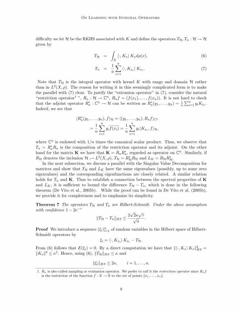
difficulty we let H be the RKHS associated with K and define the operators TH, Tn : H → Hgiven by
TH =∫X〈·,Kx〉Kxdρ(x), (6)
Tn =1n
n∑i=1
〈·,Kxi〉Kxi . (7)
Note that TH is the integral operator with kernel K with range and domain H ratherthan in L2(X, ρ). The reason for writing it in this seemingly complicated form is to makethe parallel with (7) clear. To justify the “extension operator” in (7), consider the natural“restriction operator1 ”, Rn : H → Cn, Rnf = (f(x1), . . . , f(xn)). It is not hard to checkthat the adjoint operator R∗n : Cn → H can be written as R∗n(y1, . . . , yn) = 1
n
∑ni=1 yiKxi .
Indeed, we see that
〈R∗n(y1, . . . , yn), f〉H = 〈(y1, . . . , yn), Rnf〉Cn
=1n
n∑i=1
yif(xi) =1n
n∑i=1
yi〈Kxi , f〉H,
where Cn is endowed with 1/n times the canonical scalar product. Thus, we observe thatTn = R∗nRn is the composition of the restriction operator and its adjoint. On the otherhand for the matrix K we have that K = RnR
∗n, regarded as operator on Cn. Similarly, if
RH denotes the inclusion H ↪→ L2(X, ρ), TH = R∗HRH and LK = RHR∗H.
In the next subsection, we discuss a parallel with the Singular Value Decomposition formatrices and show that TH and LK have the same eigenvalues (possibly, up to some zeroeigenvalues) and the corresponding eigenfunctions are closely related. A similar relationholds for Tn and K. Thus to establish a connection between the spectral properties of Kand LK , it is sufficient to bound the difference TH − Tn, which is done in the followingtheorem (De Vito et al., 2005b). While the proof can be found in De Vito et al. (2005b),we provide it for completeness and to emphasize its simplicity.
Theorem 7 The operators TH and Tn are Hilbert-Schmidt. Under the above assumptionwith confidence 1− 2e−τ
‖TH − Tn‖HS ≤2√
2κ√τ√
n.
Proof We introduce a sequence (ξi)ni=1 of random variables in the Hilbert space of Hilbert-Schmidt operators by
ξi = 〈·,Kxi〉Kxi − TH.
From (6) follows that E(ξi) = 0. By a direct computation we have that ‖〈·,Kx〉Kx‖2HS =‖Kx‖4 ≤ κ2. Hence, using (6), ‖TH‖HS ≤ κ and
‖ξi‖HS ≤ 2κ, i = 1, . . . , n.
1. Rn is also called sampling or evaluation operator. We prefer to call it the restriction operator since Rnfis the restriction of the function f : X → R to the set of points {x1, . . . , xn}.
9

Rosasco, Belkin, De Vito
From inequality (4) we have with probability 1− 2e−τ
‖ 1n
n∑i=1
ξi‖HS = ‖TH − Tn‖HS ≤2√
2κ√τ√
n,
which establishes the result.
As an immediate consequence of Theorem 7 we obtain several concentration results foreigenvalues and eigenfunctions discussed in subsection 3.2. However, before doing that weprovide an interpretation of the Nystrom extension based on SVD and needed to properlycompare the empirical operator and his mean.
3.1 Extension operators
We will now briefly revisit the Nystrom extension and clarify some connections to theSingular Value Decomposition (SVD) for operators. Recall that applying SVD to a p×mmatrix A produces a singular system consisting of singular (strictly positive) values (σj)kj=1
with k being the rank of A, vectors (uj)mj=1 ∈ Cm and (vj)pj=1 ∈ Cp such that they form
orthonormal bases of Cm and Cp respectively, andA∗Auj = σjuj j = 1, . . . kA∗Auj = 0 j = k + 1, . . . ,mAA∗vj = σjvj j = 1, . . . kAA∗vj = 0 j = k + 1, . . . , p.
It is not hard to see that the matrix A can be written as A = V ΣU∗, where U and V arematrices obtained by ”stacking” u’s and v’s in the columns, and Σ is a p×m matrix havingthe singular values σi on the first k-entries on the diagonal (and zero outside), so that
Auj = √σjvj j = 1, . . . kAuj = 0 j = k + 1, . . . ,mA∗vj = √σjuj j = 1, . . . kA∗vj = 0 j = k + 1, . . . , p,
which is the formulation we will use in this paper. The same formalism applies moregenerally to operators and allows us to connect the spectral properties of LK and TH aswell as the matrix K and the operator Tn. The basic idea is that each of these pairs (as shownin the previous subsection) corresponds to a singular system and thus share eigenvalues (upto some zero eigenvalues) and have eigenvectors related by a simple equation. Indeed thefollowing result can be obtained considering the SVD decomposition associated with RH(and proposition 9 considering the SVD decomposition associated with Rn). The proof ofthe following proposition can be deduced from the results in De Vito et al. (2005b, 2006)2.
2. In De Vito et al. (2005b, 2006) the results are stated for real kernels, however the proof does not changeif K is complex valued. Moreover, if K is real and LK is regarded as integral operator on the space ofsquare integrable complex functions, one can easily check that the eigenvalues are positive and, if u isan eigenfunction with eigenvalue σ ≥ 0, then the complex conjugate u is also an eigenfunction with thesame eigenvalue, so that it is always possible to choose all the eigenfunctionsto be real valued.
10

On Learning with Integral Operators
Proposition 8 The following facts hold true.
1. The operators LK and TH are positive, self-adjoint and trace class. In particular bothσ(LK) and σ(TH) are contained in [0, κ].
2. The spectra of LK and TH are the same, possibly up to the zero. If σ is a nonzeroeigenvalue and u, v are the associated eigenfunctions of LK and TH (normalized tonorm 1 in L2(X, ρ) and H) respectively, then
u(x) =1√σjv(x) for ρ-almost all x ∈ X
v(x) =1√σj
∫XK(x, s)u(s)dρ(s) for all x ∈ X
3. The following decompositions hold:
LKg =∑j≥1
σj 〈g, uj〉ρ uj g ∈ L2(X, ρ)
THf =∑j≥1
σj 〈f, vj〉 vj f ∈ H,
where the eigenfunctions (uj)j≥1 of LK form an orthonormal basis of kerLK⊥ andthe eigenfunctions (vj)j≥1 of TH form an orthonormal basis for ker(TH)⊥.
If K is real-valued, both the families (uj)j≥1 and (vj)j≥1 can be chosen as real valued func-tions.
Note that the RKHS H does not depend on the measure ρ. If the support of the measureρ is only a subset of X (e.g., a finite set of points or a submanifold), then functions inL2(X, ρ) are only defined on the support of ρ whereas functions in H are defined on thewhole space X. The eigenfunctions of LK and TH coincide (up-to a scaling factor) on thesupport of the measure, and v is an extension of u outside of the support of ρ. Moreover,the extension/restriction operations preserve both the normalization and orthogonality ofthe eigenfunctions. In a slightly different context Coifman and Lafon (2006) showed theconnection between the Nystrom method and the set of eigenfunctions of LK , which arecalled geometric harmonics. The main difference between our result and the cited paper isthat we consider all the eigenfunctions, whereas Coifman and Lafon introduce a thresholdon the spectrum to ensure stability since they do not consider a sampling procedure.
An analogous result relates the matrix K and the operator Tn .
Proposition 9 The following facts hold:
1. The operator Tn is of finite rank, self-adjoint and positive, whereas the matrix K isconjugate symmetric and semi-positive defined. In particular the spectrum σ(Tn) hasonly finitely many nonzero elements and is contained in [0, κ].
11
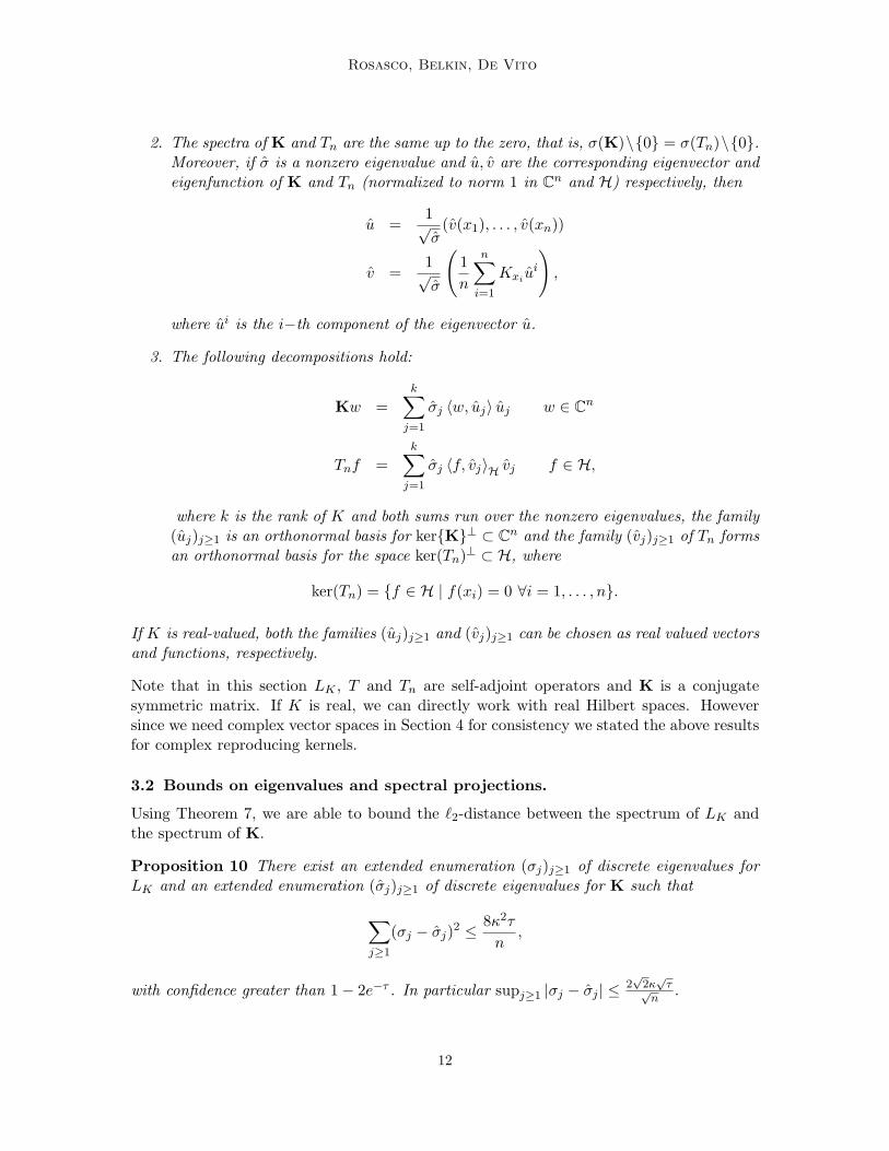
Rosasco, Belkin, De Vito
2. The spectra of K and Tn are the same up to the zero, that is, σ(K)\{0} = σ(Tn)\{0}.Moreover, if σ is a nonzero eigenvalue and u, v are the corresponding eigenvector andeigenfunction of K and Tn (normalized to norm 1 in Cn and H) respectively, then
u =1√σ
(v(x1), . . . , v(xn))
v =1√σ
(1n
n∑i=1
Kxi ui
),
where ui is the i−th component of the eigenvector u.
3. The following decompositions hold:
Kw =k∑j=1
σj 〈w, uj〉 uj w ∈ Cn
Tnf =k∑j=1
σj 〈f, vj〉H vj f ∈ H,
where k is the rank of K and both sums run over the nonzero eigenvalues, the family(uj)j≥1 is an orthonormal basis for ker{K}⊥ ⊂ Cn and the family (vj)j≥1 of Tn formsan orthonormal basis for the space ker(Tn)⊥ ⊂ H, where
ker(Tn) = {f ∈ H | f(xi) = 0 ∀i = 1, . . . , n}.
If K is real-valued, both the families (uj)j≥1 and (vj)j≥1 can be chosen as real valued vectorsand functions, respectively.
Note that in this section LK , T and Tn are self-adjoint operators and K is a conjugatesymmetric matrix. If K is real, we can directly work with real Hilbert spaces. Howeversince we need complex vector spaces in Section 4 for consistency we stated the above resultsfor complex reproducing kernels.
3.2 Bounds on eigenvalues and spectral projections.
Using Theorem 7, we are able to bound the `2-distance between the spectrum of LK andthe spectrum of K.
Proposition 10 There exist an extended enumeration (σj)j≥1 of discrete eigenvalues forLK and an extended enumeration (σj)j≥1 of discrete eigenvalues for K such that
∑j≥1
(σj − σj)2 ≤ 8κ2τ
n,
with confidence greater than 1− 2e−τ . In particular supj≥1 |σj − σj | ≤2√
2κ√τ√
n.
12

On Learning with Integral Operators
Proof By Proposition 8, an extended enumeration (σj)j≥1 of discrete eigenvalues for LK isalso an extended enumeration (σj)j≥1 of discrete eigenvalues for TH, and a similar relationholds for K and Tn by Proposition 9. Theorem 5 with A = Tn and B = TH gives that∑
j≥1
(σj − σj)2 ≤ ‖TH − Tn‖2HS
for a suitable extended enumerations (σj)j≥1, (σj)j≥1 of discrete eigenvalues for T and Tn,respectively. Theorem 7 provides us with the claimed bound.
Theorem 4.2 and the following corollaries of Koltchinskii and Gine (2000) provide the sameconvergence rate (in expectation) under a different setting (the kernel K is only symmetric,but with some assumption on the decay of the eigenvalues of LK).
The following result can be deduced by Theorem 5 with p = 1 and Theorem 7, howevera simpler direct proof is given below.
Proposition 11 Under the assumption of Proposition 10 with confidence 1− 2e−τ
|∑j≥1
(σj − σj)| = |Tr(TH)− Tr(Tn)| ≤ 2√
2κ√τ√
n.
Proof Note that
Tr(Tn) =1n
n∑i=1
K(xi, xi), and Tr(TH) =∫XK(x, x)dρ(x).
Then we can define a sequence (ξi)i=1n of real-valued random variables by ξi = K(xi, xi)−
Tr(TH). Clearly E[ξi] = 0 and |ξi| ≤ 2κ, i = 1, . . . , n so that Hoeffding inequality (3) yieldswith confidence 1− 2e−τ∣∣∣∣∣ 1n
n∑i=1
ξi
∣∣∣∣∣ = |Tr(TH)− Tr(Tn)| ≤ 2√
2κ√τ√
n.
From Proposition 6 and Theorem 7 we directly derive the probabilistic bound on the eigen-projections given by Zwald and Blanchard (2006) – their proof is based on bounded differ-ence inequality for real random variables– see also De Vito et al. (2005a). Assume for thesake of simplicity, that the cardinality of σ(LK) is infinite. Given an integer N , let m bethe sum of the multiplicities of the first N distinct eigenvalues of LK , so that
σ1 ≥ σ2 ≥ . . . ≥ σm > σm+1,
and PN be the orthogonal projection from L2(X, ρ) onto the span of the correspondingeigenfunctions. Let k be the rank of K, and u1 . . . , uk the eigenvectors corresponding tothe nonzero eigenvalues of K in a decreasing order. Denote by v1 . . . , vk ∈ H ⊂ L2(X, ρ)the corresponding Nystrom extension given by item 2 of Proposition 9.
13
Rosasco, Belkin, De Vito
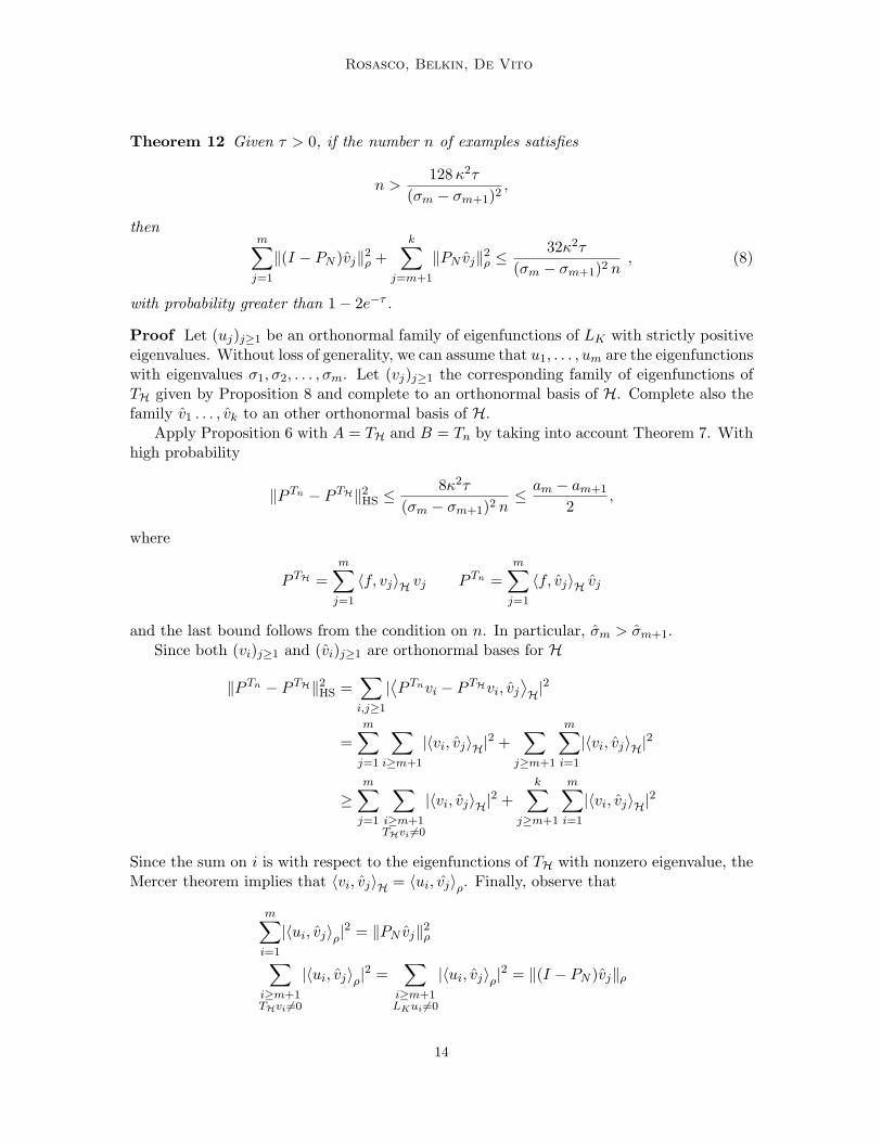
Theorem 12 Given τ > 0, if the number n of examples satisfies
n >128κ2τ
(σm − σm+1)2,
thenm∑j=1
‖(I − PN )vj‖2ρ +k∑
j=m+1
‖PN vj‖2ρ ≤32κ2τ
(σm − σm+1)2 n, (8)
with probability greater than 1− 2e−τ .
Proof Let (uj)j≥1 be an orthonormal family of eigenfunctions of LK with strictly positiveeigenvalues. Without loss of generality, we can assume that u1, . . . , um are the eigenfunctionswith eigenvalues σ1, σ2, . . . , σm. Let (vj)j≥1 the corresponding family of eigenfunctions ofTH given by Proposition 8 and complete to an orthonormal basis of H. Complete also thefamily v1 . . . , vk to an other orthonormal basis of H.
Apply Proposition 6 with A = TH and B = Tn by taking into account Theorem 7. Withhigh probability
‖P Tn − P TH‖2HS ≤8κ2τ
(σm − σm+1)2 n≤ am − am+1
2,
where
P TH =m∑j=1
〈f, vj〉H vj P Tn =m∑j=1
〈f, vj〉H vj
and the last bound follows from the condition on n. In particular, σm > σm+1.Since both (vi)j≥1 and (vi)j≥1 are orthonormal bases for H
‖P Tn − P TH‖2HS =∑i,j≥1
|⟨P Tnvi − P THvi, vj
⟩H|
2
=m∑j=1
∑i≥m+1
|〈vi, vj〉H|2 +
∑j≥m+1
m∑i=1
|〈vi, vj〉H|2
≥m∑j=1
∑i≥m+1THvi 6=0
|〈vi, vj〉H|2 +
k∑j≥m+1
m∑i=1
|〈vi, vj〉H|2
Since the sum on i is with respect to the eigenfunctions of TH with nonzero eigenvalue, theMercer theorem implies that 〈vi, vj〉H = 〈ui, vj〉ρ. Finally, observe that
m∑i=1
|〈ui, vj〉ρ|2 = ‖PN vj‖2ρ∑
i≥m+1THvi 6=0
|〈ui, vj〉ρ|2 =
∑i≥m+1LKui 6=0
|〈ui, vj〉ρ|2 = ‖(I − PN )vj‖ρ
14
On Learning with Integral Operators
where we used that kerTH ⊂ kerTn, so that vj ∈ kerLK⊥ with probability 1.
First term in the left side of inequality (19) is the projection of the vector space spannedby the Nystrom extension of the first top eigenvectors of the empirical matrix K onto theorthogonal of the vector space MN spanned by the first top eigenfunctions of the integraloperator LK , the second term is the projection of the vector space spanned by the Nystromextensions of the other eigenvectors of K ontoMN . Both differences are in L2(X, ρ) norm.A similar result is given in Zwald and Blanchard (2006), however, the role of the Nystromextensions is not considered– they study only the operators TH and Tn (with our notation).Another result similar to ours is independently given in Smale and Zhou (2008), where theauthors considered a single eigenfunction with multiplicity 1.
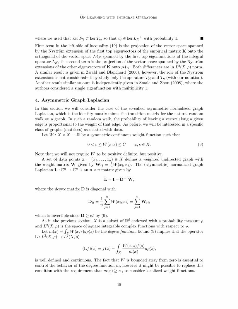
4. Asymmetric Graph Laplacian
In this section we will consider the case of the so-called asymmetric normalized graphLaplacian, which is the identity matrix minus the transition matrix for the natural randomwalk on a graph. In such a random walk, the probability of leaving a vertex along a givenedge is proportional to the weight of that edge. As before, we will be interested in a specificclass of graphs (matrices) associated with data.
Let W : X ×X → R be a symmetric continuous weight function such that
0 < c ≤W (x, s) ≤ C x, s ∈ X. (9)
Note that we will not require W to be positive definite, but positive.A set of data points x = (x1, . . . , xn) ∈ X defines a weighted undirected graph with
the weight matrix W given by Wij = 1nW (xi, xj). The (asymmetric) normalized graph
Laplacian L : Cn → Cn is an n× n matrix given by
L = I−D−1W,
where the degree matrix D is diagonal with
Dii =1n
n∑j=1
W (xi, xj) =n∑j=1
Wij ,
which is invertible since D ≥ cI by (9).As in the previous section, X is a subset of Rd endowed with a probability measure ρ
and L2(X, ρ) is the space of square integrable complex functions with respect to ρ.Let m(x) =
∫XW (x, s)dρ(s) be the degree function, bound (9) implies that the operator
L : L2(X, ρ)→ L2(X, ρ)
(Lf)(x) = f(x)−∫X
W (x, s)f(s)m(x)
dρ(s),
is well defined and continuous. The fact that W is bounded away from zero is essential tocontrol the behavior of the degree function m, however it might be possible to replace thiscondition with the requirement that m(x) ≥ c , to consider localized weight functions.
15

Rosasco, Belkin, De Vito
We see that when a set x = (x1, . . . , xn) ∈ X is sampled i.i.d. according to ρ, thematrix L is an empirical version of the operator L. We will view L as a perturbation ofL due to finite sampling and will extend the approach developed in this paper to relatetheir spectral properties. Note that the methods described in the previous section are notdirectly applicable in this setting since W is not necessarily positive definite, so there is noRKHS associated with it. Moreover, even if W is positive definite, L involves division bya function, and may not be a map from the RKHS to itself. To overcome this difficulty inour theoretical analysis, we will rely on an auxiliary RKHS H with reproducing kernel K.Interestingly enough, this space will play no role from the algorithmic point of view, butonly enters the theoretical analysis.
To state the properties of H we define the following functions
Kx : X → C Kx(t) = K(t, x)Wx : X → R Wx(t) = W (t, x)
mn : X → R mn =1n
n∑i=1
Wxi ,
where mn is the empirical counterpart of the function m and, in particular, mn(xi) = Dii.To proceed we need the following Assumption A, which postulates that the functions
wx,Wx/m,Wx/mn belong to H. However it is important to note that for W sufficientlysmooth (as we expect it to be in most applications) these conditions can be satisfied bychoosing H to be a Sobolev space of sufficiently high degree. This is made precise in theSection 4.2 (see Assumption A1).
AssumptionA Given a continuous weight function W satisfying (9), we assume thereexists a RKHS H with bounded continuous kernel K such that
Wx,1mWx,
1mn
Wx ∈ H
‖ 1mWx‖H ≤ C,
for all x ∈ X.Assumption A allows to define the following bounded operators LH, AH : H → H
AH =∫X〈·,Kx〉H
1mWx dρ(x)
LH = I −AH (10)
and their empirical counterparts Ln, An : H → H
An =1n
n∑i=1
〈·,Kxi〉H1mn
Wxi
Ln = I −An. (11)
Next result will show that LH, AH and L have related eigenvalues and eigenfunctions andthat eigenvalues and eigenfunctions (eigenvectors) of Ln, An and L are also closely related.In particular we will see in the following that to relate the spectral properties of L and L itsuffices to control the deviation AH − An. However, before doing this, we make the abovestatements precise in the following subsection.
16
On Learning with Integral Operators
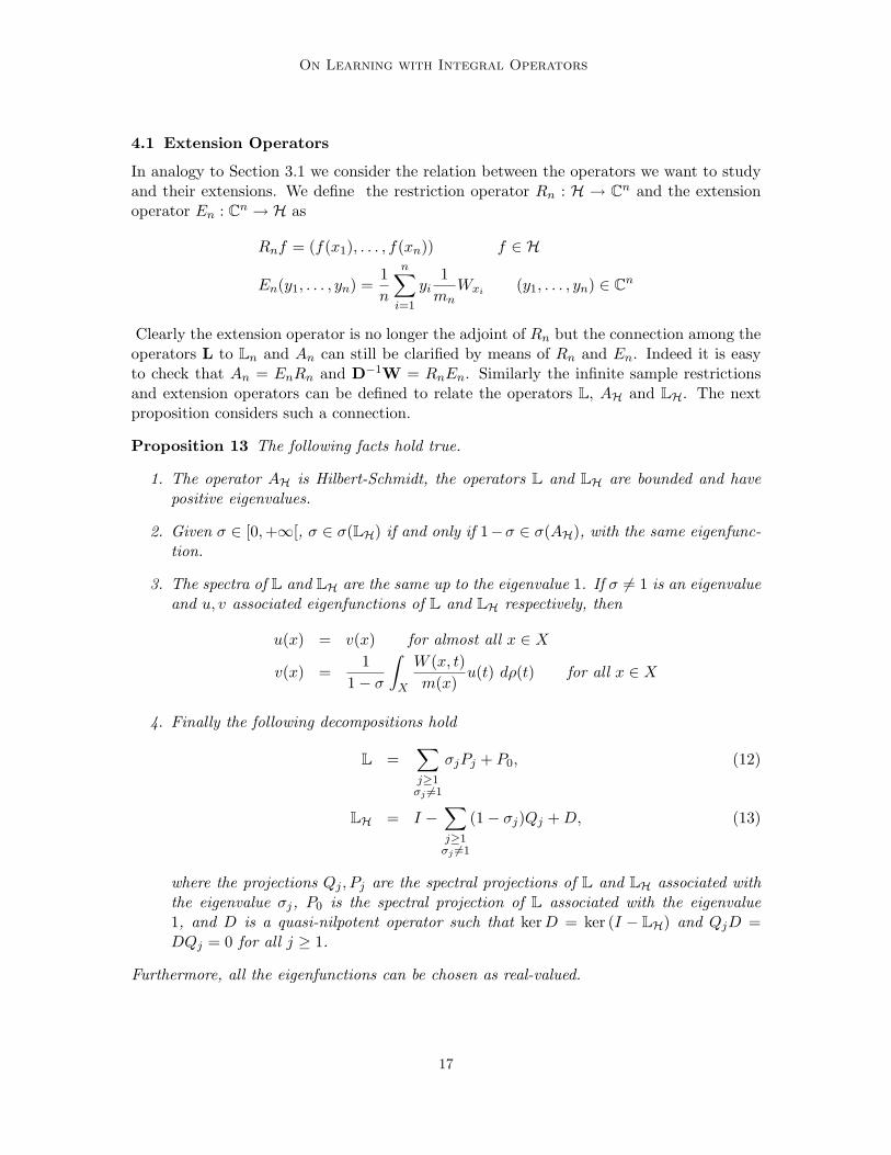
4.1 Extension Operators
In analogy to Section 3.1 we consider the relation between the operators we want to studyand their extensions. We define the restriction operator Rn : H → Cn and the extensionoperator En : Cn → H as
Rnf = (f(x1), . . . , f(xn)) f ∈ H
En(y1, . . . , yn) =1n
n∑i=1
yi1mn
Wxi (y1, . . . , yn) ∈ Cn
Clearly the extension operator is no longer the adjoint of Rn but the connection among theoperators L to Ln and An can still be clarified by means of Rn and En. Indeed it is easyto check that An = EnRn and D−1W = RnEn. Similarly the infinite sample restrictionsand extension operators can be defined to relate the operators L, AH and LH. The nextproposition considers such a connection.
Proposition 13 The following facts hold true.
1. The operator AH is Hilbert-Schmidt, the operators L and LH are bounded and havepositive eigenvalues.
2. Given σ ∈ [0,+∞[, σ ∈ σ(LH) if and only if 1−σ ∈ σ(AH), with the same eigenfunc-tion.
3. The spectra of L and LH are the same up to the eigenvalue 1. If σ 6= 1 is an eigenvalueand u, v associated eigenfunctions of L and LH respectively, then
u(x) = v(x) for almost all x ∈ X
v(x) =1
1− σ
∫X
W (x, t)m(x)
u(t) dρ(t) for all x ∈ X
4. Finally the following decompositions hold
L =∑j≥1σj 6=1
σjPj + P0, (12)
LH = I −∑j≥1σj 6=1
(1− σj)Qj +D, (13)
where the projections Qj , Pj are the spectral projections of L and LH associated withthe eigenvalue σj, P0 is the spectral projection of L associated with the eigenvalue1, and D is a quasi-nilpotent operator such that kerD = ker (I − LH) and QjD =DQj = 0 for all j ≥ 1.
Furthermore, all the eigenfunctions can be chosen as real-valued.
17

Rosasco, Belkin, De Vito
The proof of the above result is long and quite technical and can be found in Appendix A.Note that, with respect to Proposition 9, neither the normalization nor the orthogonalityis preserved by the extension/restriction operations, so that we are free to normalize vwith the factor 1/(1 − σ), instead of 1/
√1− σ as in Proposition 8. One can easily show
that, if u1, . . . , um is a linearly independent family of eigenfunctions of L with eigenvaluesσ1, . . . , σm 6= 1, then the extension v1, . . . , vm is a linearly independent family of eigenfunc-tions of LH with eigenvalues σ1, . . . , σm 6= 1. Finally, we stress that in item 4 both seriesconverge in the strong operator topology, however, though
∑j≥1 Pi = I − P0, it is not true
that∑
j≥1Qi converges to I − Q0, where Q0 is the spectral projection of LH associatedwith the eigenvalue 1. This is the reason why we need to write the decomposition of LH asin (13) instead of (12). An analogous result allows us to relate L to Ln and An.
Proposition 14 The following facts hold true.
1. The operator An is Hilbert-Schmidt, the matrix L and the operator Ln have positiveeigenvalues.
2. Given σ ∈ [0,+∞[, σ ∈ σ(Ln) if and only if 1− σ ∈ σ(An), with the same eigenfunc-tion.
3. The spectra of L and Ln are the same up to the eigenvalue 1, moreover if σ 6= 1 is aneigenvalue and the u, v eigenvector and eigenfunction of L and Ln, then
u = (v(x1), . . . , v(x1))
v(x) =1
1− σ1n
n∑i=1
W (x, xi)mn(x)
ui
where ui is the i−th component of the eigenvector u.
4. Finally the following decompositions hold
L =∑j≥1σj 6=1
σjPj + P0,
Ln =∑j≥1σj 6=1
σjQj + Q0 + D,
where the projections Qj , Pj are the spectral projections of L and Ln associated withthe eigenvalue σj, P0 and Q0 are the spectral projections of L and Ln associated withthe eigenvalue 1, and D is a quasi-nilpotent operator such that ker D = ker (I − Ln)and QjD = DQj = 0 for all j with σj 6= 1.
The last decomposition is parallel to the Jordan canonical form for (non-symmetric) matri-ces. Notice that, since the sum is finite,
∑j≥1σj 6=1
Qj + Q0 = I.
18

On Learning with Integral Operators
4.2 Graph Laplacian Convergence for Smooth Weight Functions
If the weight function W is sufficiently differentiable, we can choose the RKHS H to be asuitable Sobolev space. For the sake of simplicity, we assume that X is a bounded opensubset of Rd with a nice boundary3. Given s ∈ N, the Sobolev space Hs = Hs(X) is
Hs = {f ∈ L2(X, dx) | Dαf ∈ L2(X, dx) ∀|α| = s},
where Dαf is the (weak) derivative of f with respect to the multi-index α = (α1, . . . , αd) ∈Nd, |α| = α1 + · · · + αd and L2(X, dx) is the space of square integrable complex functionswith respect to the Lebesgue measure (Burenkov, 1998). The spaceHs is a separable Hilbertspace with respect to the scalar product
〈f, g〉Hs = 〈f, g〉L2(X,dx) +∑|α|=s
〈Dαf,Dαg〉L2(X,dx) .
Let Csb (X) be the set of continuous bounded functions such that all the (standard) deriva-tives of order s exists and are continuous bounded functions. The space Csb (X) is a Banachspace with respect to the norm
‖f‖Csb
= supx∈X|f(x)|+
∑|α|=s
supx∈X|(Dαf)(x)|.
Since X is bounded, it is clear that Csb (X) ⊂ Hs and ‖f‖Hs ≤ d‖f‖Csb, where d is a suitable
constant depending only on s. A sort of converse also holds, which will be crucial in ourapproach, see Corollary 21 of Burenkov (1998). Let l,m ∈ N such that l −m > d
2 , then
Hl ⊂ Cmb (X) ‖f‖Cmb≤ d′‖f‖Hl (14)
where d′ is a constant depending only on l and m.From Eq (14) with l = s and m = 0, we see that the Sobolev space Hs, where s =
bd/2c+ 1, is a RKHS with a continuous4 real valued bounded kernel Ks.We are ready to state our assumption on the weight function, which implies Assump-
tion A.
Assumption A1 We assume that W : X ×X → R is a positive, symmetric function suchthat
W (x, t) ≥ c > 0 ∀x, t ∈ X (15)
W ∈ Cd+1b (X ×X). (16)
As we will see, condition (16) quantifies the regularity of W we need to use Sobolev spacesas RKHS and, as usual, it critically depends on the dimension of the input space, see alsoRemark 19 below. By inspecting our proofs, (16) can be replaced by the more technicalcondition W ∈ Hd+1(X ×X).
As a consequence of Assumption A1, we are able to control the deviation of Ln fromLH.
3. The conditions are very technical and we refer to Burenkov (1998) for the precise assumptions.4. The kernel Ks is continuous on X ×X since the embedding of Hs into Cb(X) is compact, see Schwartz
(1964).
19

Rosasco, Belkin, De Vito
Theorem 15 Under the conditions of Assumption A1, with confidence 1− 2e−τ we have
‖Ln − LH‖HS = ‖AH −An‖HS ≤ C√τ√n, (17)
where ‖·‖HS is the Hilbert-Schimdt norm of an operator in the Sobolev space Hs with s =bd/2c+ 1, and C is a suitable constant.
To prove this result we need some preliminary lemmas. In the following C will be a constantthat could change from one statement to the other. The first result shows that Assump-tion A1 implies Assumption A with H = Hs and that the multiplicative operators definedby the degree function, or its empirical estimate, are bounded.
Lemma 16 There exists a suitable constant C > 0 such that
1. for all x ∈ X, Wx,1mWx,
1mnWx ∈ Hd+1 ⊂ Hs and ‖ 1
mWx‖Hs ≤ C;
2. the multiplicative operators M,Mn : Hs → Hs defined by
Mf = mf Mnf = mnf f ∈ Hs
are bounded invertible operators satisfying
‖M‖Hs,Hs , ‖M−1‖Hs,Hs , ‖Mn‖Hs,Hs , ‖M−1n ‖Hs,Hs ≤ C (18)
‖M −Mn‖Hs,Hs ≤ C‖m−mn‖Hd+1 , (19)
where ‖·‖Hs,Hs is the operator norm of an operator in the Sobolev space Hs.
Proof Let C1 = ‖W‖Cd+1b (X×X). Given x ∈ X, clearly Wx ∈ Cd+1
b (X) and, by standard
results of differential calculus, both m and mn ∈ Cd+1b (X) with
‖Wx‖Cd+1b (X), ‖m‖Cd+1
b (X), ‖mn‖Cd+1b (X) ≤ C1.
Leibniz rule for the quotient with bound (15) gives that 1m and 1
mn∈ Cd+1
b (X) with
‖ 1m‖Cd+1
b (X), ‖1mn‖Cd+1
b (X) ≤ C2,
where C2 is independent both on n and on the sample (x1, . . . , xn). Claim in item 1 isa consequence of the fact that pointwise multiplication is a continuous bilinear map onCd+1b (X), and Cd+1
b (X) ⊂ Hd+1 ⊂ Hs with
‖f‖Hs ≤ C3‖f‖Hd+1 ≤ C4‖f‖Cd+1b (X).
We claim that if g ∈ Cd+1b (X) and f ∈ Hs, then gf ∈ Hs and
‖gf‖Hs ≤ ‖g‖Hd+1‖f‖Hs .
20

On Learning with Integral Operators
Indeed, Lemma 15 of Section 4 of Burenkov (1998) with p = p2 = 2, p1 = ∞, l = s andn = d ensures that
‖gf‖Hs ≤ ‖g‖Csb (X)‖f‖Hs .
Eq. (14) with m = s and l = d+ 1 > d/2 + s = d/2 + [d/2] + 1 provides us with the claimedbound.
The content of item 2. is a consequence of the above result with g = m,mn,1m ,
1mn
, andm−mn, respectively, satisfying ‖g‖Hd+1 ≤ C4 max{C1, C2} = C5.The constant C will be the maximum among the constants Ci.
Next lemma shows that the integral operator of kernel W and its empirical counterpart areHilbert-Schmidt operators and it bounds their difference.
Lemma 17 The operators LW,H, LW,n : Hs → Hs defined by
LW,H =∫X〈·,Ks
x〉Hs Wxdρ(x),
LW,n =1n
n∑i=1
⟨·,Ks
xi
⟩Hs Wxi ,
are Hilbert-Schmidt. Furthermore, with confidence 1− 2e−τ
‖LW,H − LW,n‖HS ≤ C√τ√n.
for a suitable constant C.
Proof Note that ‖⟨·,Ks
xi
⟩Hs Wxi‖HS = ‖Ks
xi‖Hs‖Wxi‖Hs ≤ C1 for a suitable constant
C1, which is finite by item 1 of Lemma 16 and the fact that Ks is bounded. HenceLW,n, LW,H are Hilbert Schmidt operators on Hs. The random variables (ξi)ni=1 definedby ξi =
⟨·,Ks
xi
⟩Hs Wxi −LW,H, taking value in the Hilbert space of Hilbert-Schmidt opera-
tors, are zero mean and bounded. Applying (4) we have with confidence 1− 2e−τ
‖LW,H − LW,n‖HS ≤ C√τ√n, (20)
for a suitable constant C.
We then consider multiplication operators defined by the degree functions.
Lemma 18 With confidence 1− 2e−τ
‖M −Mn‖Hs,Hs ≤ C√τ√n.
for a suitable constant C.
Proof Item 2 of Lemma 16 ensures that M and Mn are bounded operators on Hs with‖M −Mn‖Hs,Hs ≤ C1‖m−mn‖Hd+1 .
21
Rosasco, Belkin, De Vito
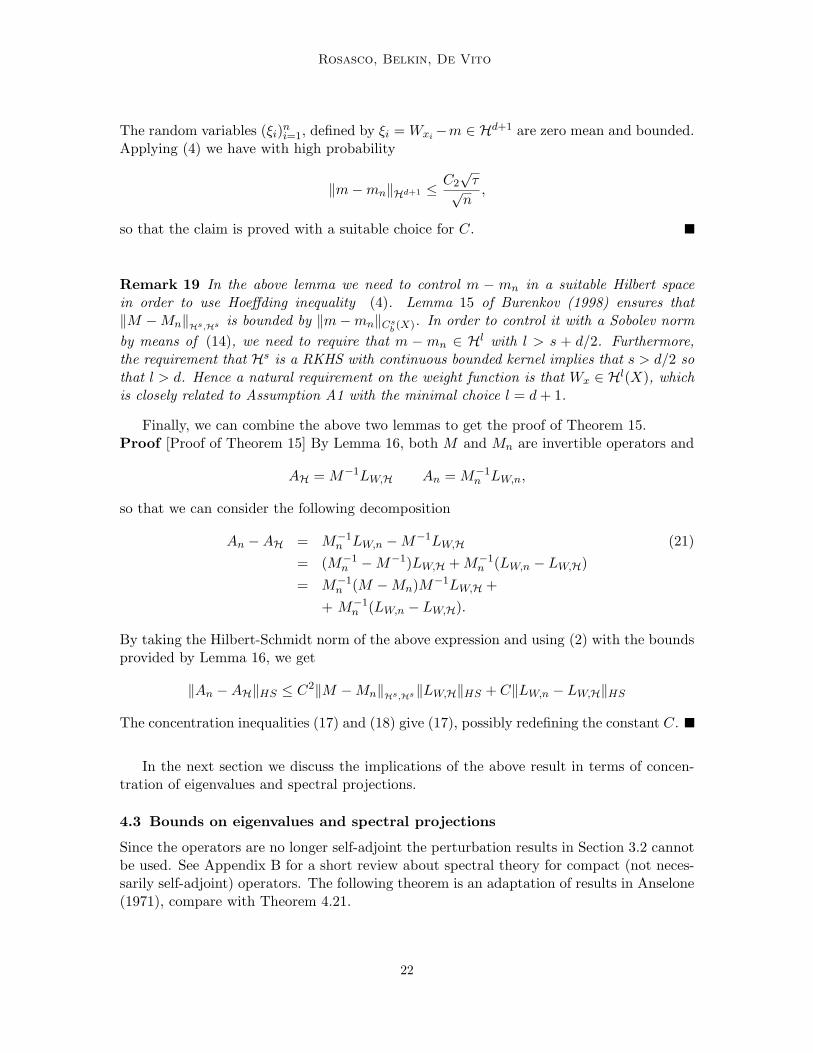
The random variables (ξi)ni=1, defined by ξi = Wxi−m ∈ Hd+1 are zero mean and bounded.Applying (4) we have with high probability
‖m−mn‖Hd+1 ≤C2√τ√n,
so that the claim is proved with a suitable choice for C.
Remark 19 In the above lemma we need to control m − mn in a suitable Hilbert spacein order to use Hoeffding inequality (4). Lemma 15 of Burenkov (1998) ensures that‖M −Mn‖Hs,Hs is bounded by ‖m−mn‖Cs
b (X). In order to control it with a Sobolev normby means of (14), we need to require that m − mn ∈ Hl with l > s + d/2. Furthermore,the requirement that Hs is a RKHS with continuous bounded kernel implies that s > d/2 sothat l > d. Hence a natural requirement on the weight function is that Wx ∈ Hl(X), whichis closely related to Assumption A1 with the minimal choice l = d+ 1.
Finally, we can combine the above two lemmas to get the proof of Theorem 15.Proof [Proof of Theorem 15] By Lemma 16, both M and Mn are invertible operators and
AH = M−1LW,H An = M−1n LW,n,
so that we can consider the following decomposition
An −AH = M−1n LW,n −M−1LW,H (21)
= (M−1n −M−1)LW,H +M−1
n (LW,n − LW,H)= M−1
n (M −Mn)M−1LW,H ++ M−1
n (LW,n − LW,H).
By taking the Hilbert-Schmidt norm of the above expression and using (2) with the boundsprovided by Lemma 16, we get
‖An −AH‖HS ≤ C2‖M −Mn‖Hs,Hs‖LW,H‖HS + C‖LW,n − LW,H‖HS
The concentration inequalities (17) and (18) give (17), possibly redefining the constant C.
In the next section we discuss the implications of the above result in terms of concen-tration of eigenvalues and spectral projections.
4.3 Bounds on eigenvalues and spectral projections
Since the operators are no longer self-adjoint the perturbation results in Section 3.2 cannotbe used. See Appendix B for a short review about spectral theory for compact (not neces-sarily self-adjoint) operators. The following theorem is an adaptation of results in Anselone(1971), compare with Theorem 4.21.
22

On Learning with Integral Operators
Theorem 20 Let A be a compact operator. Given a finite set Λ of non-zero eigenvalues ofA, let Γ be any simple rectifiable closed curve (having positive direction) with Λ inside andσ(A) \ Λ outside. Let P be the spectral projection associated with Λ, that is,
P =1
2πi
∫Γ(λ−A)−1 dλ,
and defineδ−1 = sup
λ∈Γ‖(λ−A)−1‖.
Let B be another compact operator such that
‖B −A‖ ≤ δ2
δ + `(Γ)/2π< δ,
where `(Γ) is the length of Γ, then the following facts hold true.
1. The curve Γ is a subset of the resolvent set of B enclosing a finite set Λ of non-zeroeigenvalues of B;
2. Denoting by P the spectral projection of B associated with Λ, then
‖P − P‖ ≤ `(Γ)2πδ
‖B −A‖δ − ‖B −A‖
;
3. The dimension of the range of P is equal to the dimension of the range of P .
Moreover, if B −A is a Hilbert-Schmidt operator, then
‖P − P‖HS ≤`(Γ)2πδ
‖B −A‖HSδ − ‖B −A‖
.
We postpone the proof of the above result to Appendix A.We note that, if A is self-adjoint, then the spectral theorem ensures that
δ = minλ∈Γ,σ∈Λ
|λ− σ|.
The above theorem together with the results obtained in the previous section allows toderive several results.
Proposition 21 If Assumption A1 holds, let σ be an eigenvalue of L, σ 6= 1, with mul-tiplicity m. For any ε > 0 and τ > 0, there exists an integer n0 and a positive constantC such that, if the number of examples is greater than n0, with probability greater than1− 2e−τ ,
1. there are σ1, . . . , σm (possibly repeated) eigenvalues of the matrix L satisfying
|σi − σ| ≤ ε for all i = 1, . . . ,m.
23
Rosasco, Belkin, De Vito
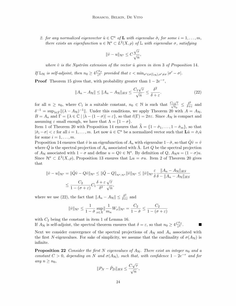
2. for any normalized eigenvector u ∈ Cn of L with eigenvalue σi for some i = 1, . . . ,m,there exists an eigenfunction u ∈ Hs ⊂ L2(X, ρ) of L with eigenvalue σ, satisfying
‖v − u‖Hs ≤ C√τ√n,
where v is the Nystrom extension of the vector u given in item 3 of Proposition 14.
If LH is self-adjoint, then n0 ≥ 4C2τε2
provided that ε < minσ′∈σ(LH),σ′ 6=σ |σ′ − σ|.
Proof Theorem 15 gives that, with probability greater than 1− 2e−τ ,
‖An −AH‖ ≤ ‖An −AH‖HS ≤C1√τ√n≤ δ2
δ + ε. (22)
for all n ≥ n0, where C1 is a suitable constant, n0 ∈ N is such that C1√τ√
n0≤ δ2
δ+ε and
δ−1 = supλ∈Γ‖(λ−AH)−1‖. Under this conditions, we apply Theorem 20 with A = AH,B = An and Γ = {λ ∈ C | |λ− (1− σ)| = ε}, so that `(Γ) = 2πε. Since AH is compact andassuming ε small enough, we have that Λ = {1− σ}.Item 1 of Theorem 20 with Proposition 14 ensures that Λ = {1− σ1, . . . , 1− σm}, so that|σi−σ| < ε for all i = 1, . . . ,m. Let now u ∈ Cn be a normalized vector such that Lu = σiufor some i = 1, . . . ,m.Proposition 14 ensures that v is an eigenfunction of An with eigenvalue 1−σ, so that Qv = vwhere Q is the spectral projection of An associated with Λ. Let Q be the spectral projectionof AH associated with 1− σ and define u = Qv ∈ Hs. By definition of Q, AHu = (1− σ)u.Since Hs ⊂ L2(X, ρ), Proposition 13 ensures that Lu = σu. Item 2 of Theorem 20 givesthat
‖v − u‖Hs = ‖Qv −Qv‖Hs ≤ ‖Q−Q‖Hs,Hs‖v‖Hs ≤ ‖v‖Hsε
δ
‖An −AH‖HSδ − ‖An −AH‖HS
≤ C2
1− (σ + ε)C1δ + ε
δ2
√τ√n,
where we use (22), the fact that ‖An −AH‖ ≤ δ2
δ+ε and
‖v‖Hs ≤ 11− σ
supx∈X‖ 1mn
Wx‖Hs =C2
1− σ≤ C2
1− (σ + ε)
with C2 being the constant in item 1 of Lemma 16.If AH is self-adjoint, the spectral theorem ensures that δ = ε, so that n0 ≥ 4C
2τε2
.
Next we consider convergence of the spectral projections of AH and An associated withthe first N -eigenvalues. For sake of simplicity, we assume that the cardinality of σ(AH) isinfinite.
Proposition 22 Consider the first N eigenvalues of AH. There exist an integer n0 and aconstant C > 0, depending on N and σ(AH), such that, with confidence 1 − 2e−τ and forany n ≥ n0,
‖PN − PD‖HS ≤C√τ√n,
24
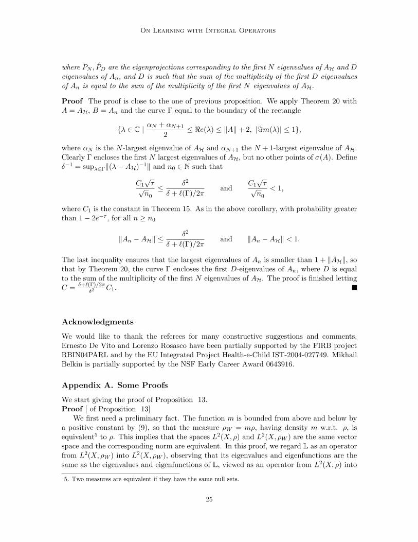
On Learning with Integral Operators
where PN , PD are the eigenprojections corresponding to the first N eigenvalues of AH and Deigenvalues of An, and D is such that the sum of the multiplicity of the first D eigenvaluesof An is equal to the sum of the multiplicity of the first N eigenvalues of AH.
Proof The proof is close to the one of previous proposition. We apply Theorem 20 withA = AH, B = An and the curve Γ equal to the boundary of the rectangle
{λ ∈ C | αN + αN+1
2≤ <e(λ) ≤ ‖A‖+ 2, |=m(λ)| ≤ 1},
where αN is the N -largest eigenvalue of AH and αN+1 the N + 1-largest eigenvalue of AH.Clearly Γ encloses the first N largest eigenvalues of AH, but no other points of σ(A). Defineδ−1 = supλ∈Γ‖(λ−AH)−1‖ and n0 ∈ N such that
C1√τ√
n0
≤ δ2
δ + `(Γ)/2πand
C1√τ√
n0
< 1,
where C1 is the constant in Theorem 15. As in the above corollary, with probability greaterthan 1− 2e−τ , for all n ≥ n0
‖An −AH‖ ≤δ2
δ + `(Γ)/2πand ‖An −AH‖ < 1.
The last inequality ensures that the largest eigenvalues of An is smaller than 1 + ‖AH‖, sothat by Theorem 20, the curve Γ encloses the first D-eigenvalues of An, where D is equalto the sum of the multiplicity of the first N eigenvalues of AH. The proof is finished lettingC = δ+`(Γ)/2π
δ2C1.
Acknowledgments
We would like to thank the referees for many constructive suggestions and comments.Ernesto De Vito and Lorenzo Rosasco have been partially supported by the FIRB projectRBIN04PARL and by the EU Integrated Project Health-e-Child IST-2004-027749. MikhailBelkin is partially supported by the NSF Early Career Award 0643916.
Appendix A. Some Proofs
We start giving the proof of Proposition 13.Proof [ of Proposition 13]
We first need a preliminary fact. The function m is bounded from above and below bya positive constant by (9), so that the measure ρW = mρ, having density m w.r.t. ρ, isequivalent5 to ρ. This implies that the spaces L2(X, ρ) and L2(X, ρW ) are the same vectorspace and the corresponding norm are equivalent. In this proof, we regard L as an operatorfrom L2(X, ρW ) into L2(X, ρW ), observing that its eigenvalues and eigenfunctions are thesame as the eigenvalues and eigenfunctions of L, viewed as an operator from L2(X, ρ) into
5. Two measures are equivalent if they have the same null sets.
25

Rosasco, Belkin, De Vito
L2(X, ρ) – however, functions that are orthogonal in L2(X, ρW ) in general are not orthogonalin L2(X, ρ).
Note that the operator IK : H → L2(X, ρW ) defined by IKf(x) = 〈f,Kx〉 is linear andHilbert-Schmidt since
‖IK‖2HS =∑j≥1
‖IKej‖2ρW=∫X
∑j≥1
〈Kx, ej〉2 dρW (x)
=∫XK(x, x)m(x) dρ(x) ≤ κ‖m‖∞,
where κ = supx∈X K(x, x). The operator I∗W : L2(X, ρW )→ H defined by
I∗W f =∫X
1mWxf(x) dρ(x)
is linear and bounded since, by Assumption A
‖∫X
1mWxf(x) dρ(x)‖H ≤
∫X‖ 1mWx‖H|f(x)| dρ(x) ≤ C‖f‖ρ ≤
C
c‖f‖ρW .
A direct computation shows that
I∗W IK = AH = I − LH σ(AH) = 1− σ(LH)
andIKI
∗W = I − L σ(IKI∗W ) = 1− σ(L).
Both I∗W IK and IKI∗W are Hilbert-Schmidt operators since they are composition of a
bounded operator and Hilbert-Schmidt operator. Moreover, let σ 6= 1 and v ∈ H withv 6= 0 such that LHv = σv. Letting u = IKv, then
Lu = (I − IKI∗W )IKv = IKLv = σu and I∗Wu = I∗W IKv = (1− σ)v 6= 0,
so that u 6= 0 and u is an eigenfunction of L with eigenvalue σ. Similarly we can prove thatif σ 6= 1 and u ∈ L2(X, ρ), u 6= 0 is such that Lu = σu, then v = 1
1−σ I∗Wu is different from
zero and is an eigenfunction of LH with eigenvalue σ.We now show that L is a positive operator on L2(X, ρW ), so that both L and LH have
positive eigenvalues. Indeed, let f ∈ L2(X, ρW ),
〈Lf, f〉ρW=
∫X|f(x)|2m(x)dρ(x)−
∫X
(∫X
W (x, s)m(x)
f(s)dρ(s))f(x)m(x)dρ(x)
=12
∫X
∫X
[|f(x)|2W (x, s)− 2W (x, s)f(x)f(s) + |f(s)|2W (x, s)
]dρ(s)dρ(x)
=12
∫X
∫XW (x, s)|f(x)− f(s)|2dρ(s)dρ(x) ≥ 0,
where we used that W (x, s) = W (s, x) > 0 and m(x) =∫XW (x, s) dρ(s). Since W is real
valued, it follows that we can always choose the eigenfunctions of L as real valued, and, asa consequence, the eigenfunctions of LH.
26

On Learning with Integral Operators
Finally we prove that both L and LH admit a decomposition in terms of spectral pro-jections – we stress that the spectral projection of L is orthogonal in L2(X, ρW ), but not inL2(X, ρ).Since L is a positive operator on L2(X, ρW ), it is self-adjoint, as well as IKI∗W , hence thespectral theorem gives
IKI∗W =
∑j≥1
(1− σj)Pj
where for all j, Pj : L2(X, ρW )→ L2(X, ρW ) is the spectral projection of IKI∗W associatedto the eigenvalue 1 − σj 6= 0. Moreover note that Pj is also the spectral projection of Lassociated to the eigenvalue σj 6= 1. By definition Pj satisfies:
P 2j = Pj ,
P ∗j = Pj the adjoint is in L2(X, ρW )PjPi = 0, i 6= j,
PjPker(IKI∗W ) = 0∑j≥1
Pj = I − Pker(IKI∗W ) = I − P0
where Pker(IKI∗W ) is the projection on the kernel of IKI∗W , that is, the projection P0. More-over the sum in the last equation converges in the strong operator topology. In particularwe have
IKI∗WPj = PjIKI
∗W = (1− σj)Pj ,
so thatL = I − IKI∗W =
∑j≥1
σjPj + P0.
Let Qj : H → H be defined by
Qj =1
1− σjI∗WPjIK .
Then from the properties of the projections Pj we have,
Q2j =
1(1− σj)2
I∗WPjIKI∗WPjIK =
11− σj
I∗WPjPjIK = Qj ,
QjQi =1
(1− σj)(1− σi)I∗WPjIKI
∗WPiIK =
11− σi
I∗WPjPiIK = 0 i 6= j.
Moreover,∑j≥1
(1− σj)Qj =∑j≥1
(1− σj)1
1− σjI∗WPjIK = I∗W (
∑j≥1
Pj)IK = I∗W IK − I∗WPker(IKI∗W )IK
so thatIKI
∗W =
∑j≥1
(1− σj)Qj + I∗WPker(IKI∗W )IK ,
27

Rosasco, Belkin, De Vito
where again all the sums are to be intended as converging in the strong operator topology.If we let D = I∗WPker(IKI∗W )IK then
QjD =1
1− σjI∗WPjIKI
∗WPker(IKI∗W ) = I∗WPjPker(IKI∗W ) = 0,
and, similarly DQj = 0. By construction σ(D) = 0, that is, D is a quasi-nilpotent operator.Equation (13) is now clear as well as the fact that kerD = ker (I − LH).
Proof [Proof of Proposition 14] The proof is the same as the above proposition by replacingρ with the empirical measure 1
n
∑ni=1 δxi .
Next we prove Theorem 20.Proof [Proof of Theorem 20] We recall the following basic result. Let S and T two boundedoperators acting on H and defined C = I − ST . If ‖C‖ < 1, then T has a bounded inverseand
T−1 − S = (I − C)−1CS
where we note that ‖I − C‖−1 ≤ 11−‖C‖ since ‖C‖ < 1, see Proposition 1.2 of Anselone
(1971).Let A and B two compact operators. Let Γ be a compact subset of the resolvent set of
A and defineδ−1 = sup
λ∈Γ‖(λ−A)−1‖,
which is finite since Γ is compact and the resolvent operator (λ−A)−1 is norm continuous,see for example Anselone (1971) . Assume that
‖B −A‖ < δ,
then for any λ ∈ Γ
‖(λ−A)−1(B −A)‖ ≤ ‖(λ−A)−1‖‖B −A‖ ≤ δ−1‖B −A‖ < 1.
Hence we can apply the above result with S = (λ−A)−1, T = (λ−B), since
C = I − (λ−A)−1(λ−B)−1 = (λ−A)−1(B −A).
It follows that (λ−B) has a bounded inverse and
(λ−B)−1 − (λ−A)−1 = (I − (λ−A)−1(B −A))−1(λ−A)−1(B −A)(λ−A)−1.
In particular, Λ is a subset of the resolvent set of B and, if B − A is a Hilbert-Schmidtoperator, so is (λ−B)−1 − (λ−A)−1.
Let Λ be a finite set of non-zero eigenvalues. Let Γ be any simple closed curve with Λinside and σ(A) \ Λ outside. Let P be the spectral projection associated with Λ, then
P =1
2πi
∫Γ(λ−A)−1 dλ.
28

On Learning with Integral Operators
Applying the above result, it follows that Γ is a subset of the resolvent set of B and we letΛ be the subset of σ(B) inside Γ and P the corresponding spectral projection, then
P − P =1
2πi
∫Γ(λ−B)−1 − (λ−A)−1 dλ
=1
2πi
∫Γ(I − (λ−A)−1(B −A))−1(λ−A)−1(B −A)(λ−A)−1 dλ.
It follows that
‖P − P‖ ≤ `(Γ)2π
δ−2‖B −A‖1− δ−1‖B −A‖
=`(Γ)2πδ
‖B −A‖δ − ‖B −A‖
.
In particular if ‖B −A‖ ≤ δ2
δ+`(Γ)/2π < δ, ‖P − P‖ ≤ 1 so that the dimension of the range
of P is equal to the dimension of the range of P . It follows that Λ is not empty.If B−A is a Hilbert-Schmidt operator, we can replace the operator norm with the Hilbert-Schmidt norm, and the corresponding inequality is a consequence of the fact that theHilbert-Schmidt operator are an ideal.
Appendix B. Spectral theorem for non-self-adjoint compact operators
Let A : H → H be a compact operator. The spectrum σ(A) of A is defined as the set ofcomplex number such that the operator(A−λI) does not admit a bounded inverse, whereasthe complement of σ(A) is called the resolvent set and denoted by ρ(A). For any λ ∈ ρ(A),R(λ) = (A − λI)−1 is the resolvent operator, which is by definition a bounded operator.We recall the main results about the spectrum of a compact operator (Kato, 1966)
Proposition 23 The spectrum of a compact operator A is a countable compact subset ofC with no accumulation point different from zero, that is,
σ(A) \ {0} = {λi | i ≥ 1, λi 6= λj if i 6= j}
with limi→∞ λi = 0 if the cardinality of σ(A) is infinite. For any i ≥ 1, λi is an eigenvalueof A, that is, there exists a nonzero vector u ∈ H such that Au = λiu. Let Γi be a rectifiableclosed simple curve (with positive direction) enclosing λi, but no other points of σ(A), thenthe operator defined by
Pλi=
12πi
∫Γi
(λI −A)−1dλ
satisfies
PλiPλj
= δijPλiand (A− λi)Pλi
= Dλifor all i, j ≥ 1,
where Dλiis a nilpotent operator such that Pλi
Dλi= Dλi
Pλi= Dλi
. In particular thedimension of the range of Pλi
is always finite.
29

Rosasco, Belkin, De Vito
We notice that Pλiis a projection onto a finite dimensional space Hλi
, which is left invariantby A. A nonzero vector u belongs to Hλi
if and only if there exists an integer m ≤ dimHλi
such that (A − λ)mu = 0, that is, u is a generalized eigenvector of A. However, if A issymmetric, for all i ≥ 1, λi ∈ R, Pλi
is an orthogonal projection and Dλi= 0 and it holds
thatA =
∑i≥1
λiPλi
where the series converges in operator norm. Moreover, if H is infinite dimensional, λ = 0is always in σ(A), but it can be or not an eigenvalue of A.
If A be a compact operator with σ(A) ⊂ [0, ‖A‖], we introduce the following notation.Denoted by pA the cardinality of σ(A) \ {0} and given an integer 1 ≤ N ≤ pA, let λ1 >λ2 > . . . , λN > 0 be the first N nonzero eigenvalues of A, sorted in a decreasing way. Wedenote by PAN the spectral projection onto all the generalized eigenvectors correspondingto the eigenvalues λ1, . . . , λN . The range of PAN is a finite-dimensional vector space, whosedimension is the sum of the algebraic multiplicity of the first N eigenvalues. Moreover
PAN =N∑j=1
Pλj=
12πi
∫Γ(λI −A)−1dλ
where Γ is a rectifiable closed simple curve (with positive direction) enclosing λ1, . . . , λN ,but no other points of σ(A).
References
P. M. Anselone. Collectively compact operator approximation theory and applications tointegral equations. Prentice-Hall Inc., Englewood Cliffs, N. J., 1971. With an appendixby Joel Davis, Prentice-Hall Series in Automatic Computation.
N. Aronszajn. Theory of reproducing kernels. Trans. Amer. Math. Soc., 68:337–404, 1950.
F. Bauer, S. Pereverzev, and L. Rosasco. On regularization algorithms in learning theory.J. Complexity, 23(1):52–72, 2007.
M. Belkin. Problems of Learning on Manifolds. PhD thesis, University of Chicago, USA,2003.
M. Belkin and P. Niyogi. Towards a theoretical foundation for Laplacian-based manifoldmethods. In Proceedings of the 18th Conference on Learning Theory (COLT), pages486–500, 2005.
M. Belkin and P. Niyogi. Convergence of Laplacian eigenmaps. In B. Scholkopf, J. Platt,and T. Hoffman, editors, Advances in Neural Information Processing Systems 19, pages129–136. MIT Press, Cambridge, MA, 2007.
V.I. Burenkov. Sobolev spaces on domains. B. G. Teubuer, Stuttgart-Leipzig, 1998.
R. R. Coifman and S. Lafon. Geometric harmonics: A novel tool for multiscale out-of-sampleextension of empirical functions. ACHA, 21:31–52, 2006.
30

On Learning with Integral Operators
E. De Vito, A. Caponnetto, and L. Rosasco. Model selection for regularized least-squaresalgorithm in learning theory. Foundations of Computational Mathematics, 5(1):59–85,February 2005a.
E. De Vito, L. Rosasco, A. Caponnetto, U. De Giovannini, and F. Odone. Learning fromexamples as an inverse problem. Journal of Machine Learning Research, 6:883–904, May2005b.
E. De Vito, L. Rosasco, and A. Caponnetto. Discretization error analysis for Tikhonovregularization. Anal. Appl. (Singap.), 4(1):81–99, 2006.
E. Gine and V. Koltchinskii. Empirical graph Laplacian approximation of Laplace-Beltramioperators: Large sample results. High Dimensional Probability, 51:238–259, 2006.
M. Hein. Uniform convergence of adaptive graph-based regularization. In Proceedings ofthe 19th Annual Conference on Learning Theory (COLT), pages 50–64, New York, 2006.Springer.
M. Hein, J-Y. Audibert, and U. von Luxburg. From graphs to manifolds - weak and strongpointwise consistency of graph Laplacians. In Proceedings of the 18th Conference onLearning Theory (COLT), pages 470–485, 2005. Student Paper Award.
T. Kato. Perturbation theory for linear operators. Springer, Berlin, 1966.
T. Kato. Variation of discrete spectra. Commun. Math. Phys., III:501–504, 1987.
V. Koltchinskii. Asymptotics of spectral projections of some random matrices approximat-ing integral operators. Progress in Probabilty, 43, 1998.
V. Koltchinskii and E. Gine. Random matrix approximation of spectra of integral op-erators. Bernoulli, 6:113–167, 2000.
S. Lafon. Diffusion Maps and Geometric Harmonics. PhD thesis, Yale University, USA,2004.
S. Lang. Real and Functional Analysis. Springer, New York, 1993.
S. Mendelson and A. Pajor. Ellipsoid approximation with random vectors. In Proceedingsof the 18th Annual Conference on Learning Theory (COLT), pages 429–433, New York,2005. Springer.
S. Mendelson and A. Pajor. On singular values of matrices with independent rows. Bernoulli,12(5):761–773, 2006.
I. Pinelis. An approach to inequalities for the distributions of infinite-dimensional martin-gales. Probability in Banach Spaces, 8, Proceedings of the 8th International Conference,pages 128–134, 1992.
L. Schwartz. Sous-espaces hilbertiens d’espaces vectoriels topologiques et noyaux associes(noyaux reproduisants). J. Analyse Math., 13:115–256, 1964. ISSN 0021-7670.
31

Rosasco, Belkin, De Vito
J. Shawe-Taylor, N. Cristianini, and J. Kandola. On the concentration of spectral prop-erties. In T. G. Dietterich, S. Becker, and Z. Ghahramani, editors, Advances in NeuralInformation Processing Systems 14, pages 511–517, Cambridge, MA, 2002. MIT Press.
J. Shawe-Taylor, C. Williams, N. Cristianini, and J. Kandola. On the eigenspectrum of thegram matrix and the generalisation error of kernel pca. to appear in IEEE Transactionson Information Theory, 51, 2004. URL http://eprints.ecs.soton.ac.uk/9779/.
A. Singer. From graph to manifold Laplacian: The convergence rate. Appl. Comput.Harmon. Anal.,, 21:128–134, 2006.
S. Smale and D.X. Zhou. Learning theory estimates via integral operators and their ap-proximations. submitted, 2005. retrievable at http://www.tti-c.org/smale.html.
S. Smale and D.X. Zhou. Geometry of probability spaces. preprint, 2008. retrievable athttp://www.tti-c.org/smale.html.
U. Von Luxburg, O. Bousquet, and M. Belkin. On the convergence of spectral clusteringon random samples: the normalized case. In Proceedings of the 17th Annual Conferenceon Learning Theory (COLT 2004, pages 457–471. Springer, 2004.
U. von Luxburg, M. Belkin, and O. Bousquet. Consistency of spectral clustering. Ann.Statist., 36(2):555–586, 2008.
Y. Yao, L. Rosasco, and A. Caponnetto. On early stopping in gradient descent learning.Constr. Approx., 26(2):289–315, 2007.
L. Zwald and G. Blanchard. On the convergence of eigenspaces in kernel principal compo-nent analysis. In NIPS, 2006.
Laurent Zwald, Olivier Bousquet, and Gilles Blanchard. Statistical properties of kernel prin-cipal component analysis. In Learning theory, volume 3120 of Lecture Notes in Comput.Sci., pages 594–608. Springer, Berlin, 2004.
32