Extending Ozone‐Precursor Relationships in ChinaFrom Peak Concentration to Peak TimeHang Qu1 , Yuhang Wang1 , Ruixiong Zhang1 , and Jianfeng Li1

1School of Earth and Atmospheric Sciences, Georgia Institute of Technology, Atlanta, GA, USA

Abstract High ozone concentrations have become the major summertime air quality problem inChina. Extensive in situ observations are deployed for developing strategies to effectively control theemissions of ozone precursors, that is, nitrogen oxides (NOX = NO + NO2) and volatile organic compounds(VOCs). The modeling analysis of in situ observations often makes uses of the dependence of ozone peakconcentration on NOX and VOC emissions, because ozone observations are among the most widelyavailable air quality measurements. To extract more information from regulatory ozone observations, weextend the ozone‐precursor relationship to ozone peak time in this study. We find that the sensitivities ofozone peak time and concentration are complementary for regions with large anthropogenic emissionssuch as China. The ozone peak time is sensitive to both VOC and NOX emissions, and the sensitivity isnearly linear in the transition regime of ozone production compared to the changing ozone peak con-centration sensitivity in this regime, making the diagnostics of ozone peak time particularly valuable. Theextended ozone‐precursor relationships can be readily applied to understand the effects on ozoneby emission changes of NOX and VOC and to assess potential biases of NOX and VOC emissioninventories. These observation constraints based on regulatory ozone observations can complement theother measurement and modeling analysis methods nicely. Furthermore, we suggest that the ozone peaktime sensitivity we discussed here to be used as a model evaluation measure before the empiricalkinetic modeling approach (EKMA) diagram is applied to understand the effectiveness of emission controlon ozone concentrations.

Plain Language Summary High ozone concentrations have become the major summertime airquality problem in China. Air quality models are routinely used to investigate effective ozone strategies bycontrolling the emissions of ozone precursors, nitrogen oxides (NOX = NO + NO2) and volatile organiccompounds (VOCs). Therefore, the evaluations of model‐simulated sensitivities of ozone to its precursoremissions using available observations are urgently needed. In the past, efforts have been focused onsensitivities of ozone peak concentrations to its precursor emissions. We show in this work that theobservations of ozone peak time can also be applied to understand ozone sensitivities to its precursoremissions, especially in regions with large anthropogenic emissions such as China. Before air quality modelsare applied to investigate effective strategies of controlling ozone precursor emissions, we suggest that themodel simulations of ozone peak time and concentrations are evaluated using the extensive regulatoryair quality monitoring network data. Model biases in simulated ozone peak time or concentrations alsoprovide important clues to potential model errors, such as systematic biases in the estimated emissions ofozone precursors. These biases in model simulations can lead to erroneous emission control strategies andneed to be corrected before air quality models can be used in policy applications.

1. Introduction

Ground‐level ozone is a secondary air pollutant that damages human and vegetation health (U.S.EPA, 2013). The chemical production of ground‐level ozone involves the photochemical reactions betweennitrogen oxides (NOX = NO + NO2) and volatile organic compounds (VOCs) (Seinfeld & Pandis, 2016). Theozone‐precursor relationship, that is, the sensitivity of ozone to NOX and VOC emissions, is an importantfactor in establishing effective ozone control strategies (Blanchard & Fairley, 2001; Geng et al., 2008;Jimenez & Baldasano, 2004; Liu et al., 2012; Parra et al., 2009; Ren et al., 2013; Yang et al., 2011; Zhaoet al., 2009). In China megacity clusters, ozone production is often in the transition regime (Jin &Holloway, 2015; Li et al., 2013; Liu et al., 2012; Ran et al., 2009; Xing et al., 2011).

©2020. American Geophysical Union.All Rights Reserved.

RESEARCH ARTICLE10.1029/2020JD033670

Key Points:• The ozone peak time can be used

similarly to ozone peak levels toevaluate ozone sensitivities to NOX

and VOC emissions in modelsimulations

• The sensitivities of ozone peak timeand concentration arecomplementary for regions withlarge anthropogenic emissions

• The biases of model‐simulatedozone peak time and concentrationsprovide additional constraints onNOX and VOC emission inventories

Supporting Information:• Supporting Information S1

Correspondence to:Y. Wang,yuhang.wang@eas.gatech.edu

Citation:Qu, H., Wang, Y., Zhang, R., & Li, J.(2020). Extending ozone‐precursorrelationships in China from peak con-centration to peak time. Journal ofGeophysical Research: Atmospheres,125, e2020JD033670. https://doi.org/10.1029/2020JD033670

Received 7 AUG 2020Accepted 19 OCT 2020Accepted article online 23 OCT 2020

Author Contributions:Conceptualization:Hang Qu, YuhangWangFormal analysis: Hang Qu, YuhangWangMethodology: Hang Qu, RuixiongZhangSoftware: Hang Qu, Ruixiong ZhangValidation:Hang Qu, Ruixiong Zhang,Jianfeng LiVisualization: Hang QuWriting ‐ original draft: Hang Qu,Yuhang Wang

QU ET AL. 1 of 16

China is experiencing high levels of ozone due to high precursor emissions in association with rapid urba-nization and industrialization (Duncan et al., 2016; Lin et al., 2013; Ma et al., 2019; Sun et al., 2019; Wanget al., 2017; Zhao et al., 2013). In July 2018, for example, ozone was the dominant air pollutant in 155 ofthe 168 major cities in China, and in 104 of them, the maximum daily 8‐hr average (MDA8) ozone exceeds160 μg m−3 (~80 ppbv, the Grade II national air quality standard of China) (CNEMC, 2018). Ozone has beenincreasing by 1–3 ppbv yr−1 in urban and background regions in China recently (Gao et al., 2017; K. Li et al.,2019; Ma et al., 2016). In this fast‐changing environment, observation constraints are sorely needed onprecursor emissions used in the model and model‐based emission control strategies.

Diagnosing ozone sensitivity to precursor emissions often requires intensive field observations of a suite ofchemical species (e.g., Liu et al., 2012; Lu et al., 2017). When the extensive field measurements are unavail-able, it is often desirable to use the observations from the regulatory monitoring networks. The benefit is thatthese networks cover vast regions in a nation, but the limitation is that precursor measurements either haveissues or are unavailable (e.g., J. Li et al., 2019). High‐quality measurements of ozone are readily availablefrom these networks (e.g., Lu et al., 2018). A commonly used ozone‐precursor relationship is the dependenceof peak concentration of daytime ozone on NOX and VOC emissions, which is also known as the empiricalkinetic modeling approach (EKMA) diagram (e.g., Ashok & Barrett, 2016; Kinosian, 1982; Tan et al., 2018).For regulatory application purposes, it is natural to focus on peak ozone concentrations. However, from thepoint of view of modeling diagnostics and making use of the extensive ozone observations from monitoringnetworks, ozone peak time is also of interest. Previous studies showed that the spatial and temporal distri-butions over the cities (Wang et al., 2017; Yang et al., 2020) and model simulations revealed that the peaktime of the average diurnal profile of ozone responds to VOC or NOX emissions (Karl et al., 2019; J. Liet al., 2019; Ojha et al., 2012).

In this study, we extend the ozone‐precursor relationship to ozone peak time and investigate the potential ofusing extensive ozone observations in China to improve observation constraints on model simulated ozone‐precursor relationships (J. Li et al., 2019). We use the observations of ozone in July 2014 as an example todemonstrate this potential. We show that ozone peak time's dependence on NOX and VOC emissions offersnew constraints on the emissions that are different from those placed by the observed peak concentrations.Therefore, the discrepancies between simulated and observed ozone peak time and peak concentrations canbe applied to understand the biases in ozone precursor emission inventories and provide pertinent guidanceon adjusting model‐based emission control strategies.

2. Data and Methods2.1. The China National Environmental Monitoring Center (CNEMC) Network

CNEMC has established ambient atmosphere quality monitoring networks across the country since 2013,reporting hourly real‐time data of six criteria pollutants (O3, CO, NO2, SO2, PM2.5, and PM10) and air qualityindex (AQI) in cities online (http://www.cnemc.cn). The data were used in recent studies for analyzing thecurrent air quality issues (K. Li et al., 2019; Liu et al., 2018; Lu et al., 2018). In this work, we analyzed thehourly surface ozone observations from 861 sites in 189 cities for July 2014. For each site, we remove allthe data that are higher than four times the monthly average of 3‐hr running mean data for the hour ofthe observations. We then group the data by the hour of the observation and apply Tukey's fences to removeoutliers. Specifically, we remove the outlier data which are outside the range of Q1 − k(Q3 − Q1) and Q3+k(Q3−Q1), whereQ1 andQ3 are the 25th and 75th quartiles, respectively, and k= 1.5 (Tukey, 1977). A total of2.3% of the measurement data are removed. Comparison with another data quality control method(Lu et al., 2018) and no data quality control shows that the regional mean ozone peak time and peak concen-tration values are insensitive to the quality control method used (Text S1 and Figures S1 and S2 in the sup-porting information). The results presented in this work change negligibly when all the observation data areused. For each city, processed hourly observation data are first averaged over all sites, and peak time andpeak concentration of ozone are then calculated separately for each city in each day. The days with missingdaytime (8 a.m. to 8 p.m. in local Sun time) hourly data are excluded in the peak value analysis. The peaktime of ozone is converted to local Sun time based on the longitude of the city. If a computed daily peak timeof ozone occurs at nighttime (8 p.m. to 8 a.m. in local Sun time), manual inspection is made either to discardthe data or to recalculate the daytime ozone peaks for that day. The resulting daily data for each city are used

10.1029/2020JD033670Journal of Geophysical Research: Atmospheres

QU ET AL. 2 of 16

to compute regional averages. Model results for cities with corresponding observation data are processed inthe same manner.

2.2. The 3‐D Regional Chemical Transport Model

The 3‐D Regional chEmical trAnsport Model (REAM) has been widely used in studies over North America,East Asia, and other regions (Gu et al., 2014; Liu, Wang, Vrekoussis, et al., 2012; Liu et al., 2014; Wanget al., 2006, 2007; Xu et al., 2018; Zeng et al., 2006; Zhang et al., 2016; R. Zhang et al., 2017, 2018; Zhao,Wang, Choi, et al., 2009). The horizontal resolution of the model is 36 kmwith 30 vertical layers in the tropo-sphere. Meteorological data are obtained from the Weather Research and Forecasting model (WRF 3.6)assimilations constrained by the National Centers for Environmental Prediction Climate Forecast SystemVersion 2 (NCEP CFSv2) products (Saha et al., 2013). The boundary conditions for chemical tracers areobtained from the GEOS‐Chem model (v9–02) (Bey et al., 2001). The chemistry mechanism extends theGEOS‐Chem chemistry mechanism with reactions involving aromatics, ethylene, and acetylene. TheMultiresolution Emission Inventory for China (MEIC, http://www.meicmodel.org/) emissions for the year2012 are adopted in the model for anthropogenic emissions of NOX, VOCs, and CO (Li et al., 2017). Theemissions are scaled by the diurnal ratio taken from the National Emissions Inventory (NEI), and there isno weekday‐to‐weekend variation. Biogenic emissions of isoprene are calculated using the Model ofEmissions of Gases and Aerosols from Nature (MEGAN v2.1) (Guenther et al., 2012). We run the modelfor July 2014, the same period as the data we used. The model is spun up for 10 days for initialization.

A 0‐D box model is also developed based on the 3‐D REAM. The 0‐D box model uses the same chemicalmechanism as the 3‐DREAMmodel. The meteorological, physical, and chemical parameters including tem-perature, pressure, water concentration, boundary layer height, photolysis rates, deposition rates, and aero-sol surface area are averaged hourly for city grid cells with surface ozone observations. Advection transport isspecified with a transport lifetime of 5.3 hr, corresponding to an average city scale of 100 km and an averagewind speed of 5.2 m s−1. Hourly background concentrations for ozone are set at the fifth percentile value ofthe observations. Hourly backgrounds of other chemical tracers are set at the fifth percentile values of 3‐DREAM results. Each simulation is run until a steady state is reached when the differences in ozone peak con-centration and time converge to <1% from the results of the previous day. A total of 400 simulations wereconducted for NOX emissions in the range of 0–4.5 × 1016 molecules m−2 s−1 and VOC emissions in therange of 0–1.4 × 1017 molecules m−2 s−1; NOX and VOC emissions are evenly divided into 20 bins each.The upper limits of NOX and VOC emission ranges correspond to three times of average MEIC emissionsfor the cities with surface ozone observations.

3. Results3.1. Correlations of O3 Peak Concentration and Time to NOX and VOC Emissions

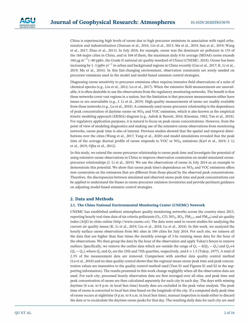
The ozone‐precursor relationships to be studied can be simply illustrated by the correspondence of ozonepeak time and concentration to NOX and VOC emissions in China. Figures 1a and 1b show the correlationsbetween ozone peak concentration and NOX and VOC emissions, respectively. The correlation coefficientsof ozone peak concentration with NOX and VOC emissions are comparable at 0.54 and 0.53, respectively. Insmall cities with NOX emissions <1 × 1015 molecules m−2 s−1, the transport processes dominate the concen-trations of ozone and its precursors, and we remove these four sites (3%) of Beihai, Zhangjiajie, Weihai, andLhasa to focus on the effects of local ozone photochemistry. Figure 1c shows that the observed ozone peaktime correlates well with MEIC NOX emission (R = 0.61) in the cities with strong NOX emissions (>1 × 1015

molecules m−2 s−1). The ozone peak time delays from 1–3 to 4–6 pm as the NOX emissions increase from1 × 1015 to 1 × 1017 molecules m−2 s−1. The ozone peak time is also correlated with VOC emission withan R value of 0.56 (Figure 1d). Figure 1 implies that the EKMA‐type relationship between ozone peak con-centration and its precursor emissions may be extended to ozone peak concentration in China.

3.2. Modeling Analysis of the Observations

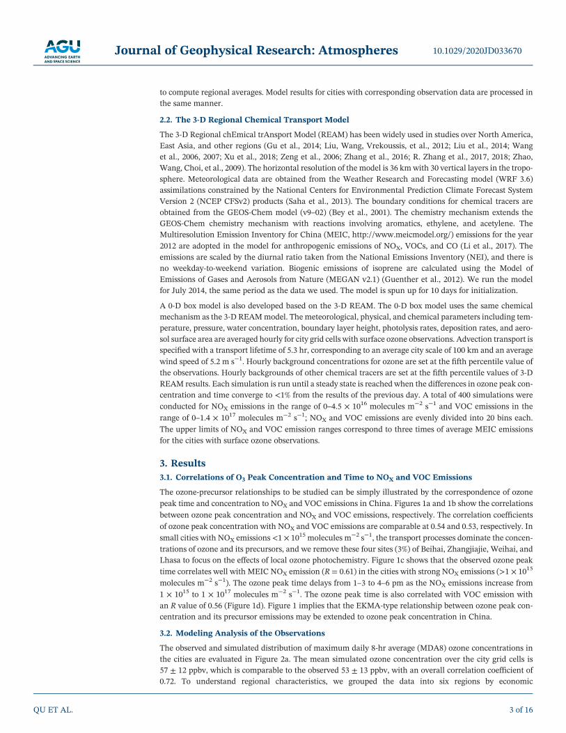
The observed and simulated distribution of maximum daily 8‐hr average (MDA8) ozone concentrations inthe cities are evaluated in Figure 2a. The mean simulated ozone concentration over the city grid cells is57 ± 12 ppbv, which is comparable to the observed 53 ± 13 ppbv, with an overall correlation coefficient of0.72. To understand regional characteristics, we grouped the data into six regions by economic

10.1029/2020JD033670Journal of Geophysical Research: Atmospheres

QU ET AL. 3 of 16

development and topography (Figure 2b): North Central Plain (NCP), Northeast (NE) region, Yangtze RiverDelta (YRD), Northwest (NW) region, Southwest (SW) region, and Pearl River Delta (PRD). Table 1summarizes the regional statistics. The observed mean MDA8 ozone concentrations range from 41 to64 ppbv in the six regions. The highest mean ozone concentration occurs in the NCP region, and thelowest mean concentration occurs in the PRD region. The model results differ from the observations by0–13 ppbv in the six regions, and the correlation coefficients between observed and simulated ozone rangefrom 0.61 to 0.81.

The comparisons of the monthly means of the simulated and observed ozone peak concentration and peaktime are illustrated in Figures 2c and 2d. Both the observed and simulated monthly mean ozone peak con-centrations in the cities are in the range of 20–90 ppbv, and they are strongly correlated with a R value of0.71. Most of the simulation results lie between the 1:2 and 2:1 lines with some exceptions in the SW andYRD regions, where the simulated peak ozone concentrations are overestimated. The ozone peak concentra-tions are highest in the NCP region and lowest in the PRD region. The observed and simulated ozone peaktime data are moderately correlated with R = 0.51, and the range of the ozone peak time is mostly from 2 to

Figure 1. Observed ozone peak concentration and time as a function of NOXand VOC emissions in the MEIC inventory,respectively, for July 2014. The pink triangles denote urban regions with NOXemissions <1015molecules m−2 s−1, whichare excluded from this study. The red line is a least squares regression for urban regions with NOXemissions>1015molecules m−2 s−1.

10.1029/2020JD033670Journal of Geophysical Research: Atmospheres

QU ET AL. 4 of 16

6 p.m. The simulated ozone peak time data in 150 cities lie within 1 hr of the observed ozone peak time. Thecities in the NCP region tend to have late afternoon (3 to 6 p.m.) ozone peaks while the cities in the PRDregion tend to have early afternoon (1 to 4 p.m.) ozone peaks.

The regional day‐to‐day variability of observed and simulated data is also compared for ozone peak concen-tration (Figure S3) and peak time (Figure S4), and the overall time series is illustrated in Figure S5. The

Figure 2. Panel (a) shows the simulated (background) and observed (circle) maximum daily 8‐hr average ozone(MDA8 O3) concentrations for July 2014. Panel (b) shows the six regions: northwest (“NW”, orange), North ChinaPlain (“NCP”, red), northeast (“NE”, green), southwest (“SW”, purple), Pearl River Delta (“PRD”, blue), and YangtzeRiver Delta (“YRD”, yellow). Panel (c) shows the comparison between observed and simulated monthly meanozone peak concentrations in the cities, and the data are color‐coded by region. The horizonal and vertical bars denotethe observed and simulated standard deviations, respectively. The red solid line corresponds to 1:1, and the reddashed lines are for 1:2 and 2:1. Panel (d) is the same as (c) but for monthly mean ozone peak time. The red solid linecorresponds to 1:1, and the red dashed lines correspond to 1‐hr difference from the 1:1 line.

Table 1Statistics of Observed and Simulated Means and Standard Deviations (ppbv) of MDA8 Ozone in Six Regions for July 2014

NCP NE NW PRD YRD SW Overall

Observations 64 ± 9 56 ± 9 55 ± 11 41 ± 11 52 ± 8 43 ± 12 53 ± 13Simulations 64 ± 8 59 ± 9 55 ± 6 42 ± 6 58 ± 12 56 ± 14 57 ± 12Correlation coefficient 0.61 0.78 0.72 0.81 0.62 0.67 0.72

10.1029/2020JD033670Journal of Geophysical Research: Atmospheres

QU ET AL. 5 of 16

ozone peak concentration data show high correlations between the observations and simulation results,indicating that the model can capture the day‐to‐day variance of the ozone peak concentrations reasonablywell. However, the correlation between the observed and simulated ozone peak time is low. The low correla-tion is due in part to the small daily ozone peak variation in a region since the square of R is inversely pro-portional to the total sum of the data variance. For the overall time series. The median of the differencebetween the simulated and observed ozone peak time is 0.14 hr.

The observed and simulated daytime (10 a.m. to 4 p.m.) NO2 concentrations are compared in Figures S6 andS7. The correlation coefficient between observed and simulated NO2 is 0.56 for city‐to‐city variability and0.43 for day‐to‐day variability, respectively. The day‐to‐day variability is higher (0.58–0.85) in the NCP,NE, PRD, and YRD regions and lower (0.48) in the NW and SW regions. Previous studies have shown thatthe surface measurements of NO2 have high biases due to the interferences of other reactive nitrogen speciessuch as peroxyacetyl nitrate (PAN) and nitric acid (HNO3) and suggested a correction factor of 0.5 to theobservation data in July in the United States (Lamsal et al., 2008; R. Zhang et al., 2018). However, inChina, a ratio of 0.80 has been found between the satellite‐derived surface NO2 and CNEMCmeasurementsin July (Gu et al., 2017). In this research, the ratio between the simulated and observed averaged NO2 is 0.72,similar to Gu et al. (2017). Given the much shorter lifetime of NOX than ozone in the summer, surface mea-surements of the former can be strongly affected by nearby local sources. The general lack of spatial repre-sentativeness of urban NO2 measurements also contributes to the differences between observed andsimulated surface NO2 concentrations.

To further investigate the relationships of ozone peak concentration and time with NOX and VOC emissions,we conduct two series of sensitivity tests: (1) NOX emissions changing from − 50% to + 50% with an

Figure 3. Sensitivities of ozone daily peak concentration and peak time to VOCs and NOXemissions in the six regions forJuly 2014. The black open circles and lines show the observed peak averages and the corresponding standard deviations.The open circles at the intersection of the red and blue lines denote the standard simulation results. The red lineswith solid dots show the sensitivities to NOXemissions (“NOXSens”); the blue lines with solid dots show the sensitivitiesof VOC emissions (“VOC Sens”). The signs of “+” and “−” denote an increase and decrease of the precursor emission inthe model, respectively. Each dot denotes an increment or decrement of 10% in emissions. Sensitivities up to plus orminus 50% are shown.

10.1029/2020JD033670Journal of Geophysical Research: Atmospheres

QU ET AL. 6 of 16

increment of 10% and (2) VOC emissions changing from − 50% to + 50% with an increment of 10%. Figure 3shows the monthly mean results of the sensitivity simulations in comparison with the observations. VOCemissions enhance the ozone peak concentration nearly linearly, while the NOX emissions affect theozone peak concentration differently. In the NW and SW regions, the ozone peak concentration increaseswith NOX emissions, but the sensitivity decreases with increasing NOX emissions. The peak ozone andNOX emission relationship is no longer monotonic in the other four regions. While increasing NOX

emissions decrease the ozone peaks, decreasing NOX emissions eventually also decrease the ozone peaks,but the turnover points are shifted to the left in the NCP, YRD, and NE regions. The sensitivity results ofthe ozone concentration to the emissions agree with previous studies (Li et al., 2013; Xing et al., 2011).

In contrast to the complex ozone peak concentration sensitivities to NOX emissions, the sensitivities of ozonepeak time to NOX and VOC are monotonic. Increasing NOX emissions delays the ozone peak time whileincreasing VOC emissions advances the ozone peak time in all six regions. For the same 50% change of emis-sions, the effect of NOX is larger than VOCs, which partly explains the higher correlation coefficient betweenozone peak time and NOX emissions than those between ozone peak time and VOC emissions or for ozonepeak concentration.

The monotonic sensitivities of ozone peak time to NOX and VOC emissions compared to the more complexresponse of ozone peak concentration to emissions imply that the observations of ozone peak time providegood constraints on model simulations other than the observations of ozone peak concentration. It is onlybecause the ambient ozone standard is based on concentrations that the observations of ozone peak timeare usually not applied to evaluate model simulations. A further useful property of the simulated ozone

Figure 4. The sensitivities of simulated ozone peak time to NOXand VOC emissions for July 2014. N + : increaseNOXemissions by 50%; N− : decrease NOXemissions by 50%; V + : increase VOC emissions by 50%; V− : decreaseVOC emissions by 50%; N +V+ : increase both NOXand VOC emissions by 50%; N−V− : decrease both NOXand VOCemissions by 50%; N +V− : increase NOXemissions by 50% and decrease VOC emissions by 50%; and N−V+ : decreaseNOXemissions by 50% and increase VOC emissions by 50%.

10.1029/2020JD033670Journal of Geophysical Research: Atmospheres

QU ET AL. 7 of 16

peak time is that the impact of changing NOX and VOC emissions concurrently by 50% is nearly additive(Figure 4): The change of ozone peak time in a simulation of changing NOX and VOC emissions by 50%concurrently is close to the sum of the simulated changes of changing NOX or VOC emissions by 50%alone. This additive effect does not exist in the ozone peak concentration simulations due to chemicalnonlinearity (Figure 5), suggesting that the observed and simulated sensitivities of ozone peak time areeasier to interpret than ozone peak concentration in urban regions of China.

We examine in more detailed chemical processes leading to these sensitivity results. The chemical produc-tion of ozone is due to the oxidation of NO by the hydroperoxy (HO2) radicals or organic peroxy (RO2) radi-cals. Peroxy radicals are mostly produced from the reactions of VOCs with OH. Photolysis of oxygenatedVOCs (OVOCs) is also a large primary source of peroxy radicals in polluted urban regions. The reaction ofOH with NO2 is a large sink of radicals and NOX (Liu et al., 2012). The sensitivities of OH, HO2 + RO2,and NOX and the rates of OVOC photolysis, the reaction rate of OH and NO2, and chemical production rateof O3 (pO3) to 50% changes of NOX or VOCs are shown in Figure 6. The sensitivity results show that NOX andVOC emissions affect ozone peak concentration and peak time in different ways. A 50% increase of NOX

emissions increases the radical sink through the reaction of OH and NO2, suppressing radical concentra-tions. The net effect is a decrease in ozone production and peak ozone concentration. A 50% decrease ofNOX emissions has the opposite consequence. The radical suppressing effect by an increase of NOX is largerin the early morning when the primary radical source is smaller than at noon. As a result, the ramping up ofozone production is delayed, and the ozone peak time is later. A 50% increase of VOC emissions increasesHO2 and RO2 concentrations but does not affect NOX concentrations as much, thereby increasing ozone pro-duction and peak concentrations. The effect of VOC emissions on ozone peak time is largely due to the reac-tions of the VOCs with the OH radical (Figure S8) and the photolysis of OVOCs, both of which peak before orat noon, while ozone peak time is in midafternoon (Figure 3). A 50% increase of VOC emissions increases

Figure 5. The same as Figure 4 but for ozone peak concentration.

10.1029/2020JD033670Journal of Geophysical Research: Atmospheres

QU ET AL. 8 of 16

OVOC photolysis, shifting HO2 and RO2 concentration peak toward noon and making ozone peak timeoccurs in earlier afternoon. Similarly, a 50% decrease of VOC emissions delays ozone peak time.

3.3. Isopleth Diagram for Ozone Peak Time

The EKMA isopleth diagram for the sensitivity of ozone to NOX and VOC emissions has been widely used(Ashok & Barrett, 2016; Kinosian, 1982; Sillman et al., 1990; Sillman & Samson, 1993; Tan et al., 2018).We use the 0‐D box model to compute the EKMA‐type diagrams for ozone peak concentration and timefor the urban regions of China in this study. Averaged hourly regional transport time, deposition rates, back-ground concentrations, wind speed, and boundary layer height are included to simulate the effect of advec-tion, mixing, and deposition. The results provide qualitative guidance on understanding the 3‐D modelresults discussed previously.

Figure 7a shows the sensitivity diagrams for peak ozone concentration. The peak ozone sensitivity diagramis as expected. Under high NOX and lowVOC emissions, peak ozone concentration increases with increasingVOC and decreasing NOX emissions, although the VOC sensitivity is much higher than NOX. Hence, it isoften referred to as the VOC‐limited regime. Under low NOX and high VOC emissions, which is oftenreferred to as the NOX‐limited regime, peak ozone concentration increases with increasing NOX emissionsrapidly but is insensitive to VOC emissions. In the transition regime (near the area between the two dashedred lines in Figure 7), peak ozone concentration increases with increasing NOX or VOC emissions. If theVOC to NOX emission ratio (C:N ratio) decreases to the lower right of the diagram, the sensitivity of peak

Figure 6. Sensitivities of OH, HO2 + RO2, NOX, and the rates of OVOC photolysis, the reaction rate of OH and NO2, and pO3to 50% changes of NOXor VOCs aturban sites in this study for July 2014. The black lines are the results from the standard model; the red dashed lines show the results from a 50% increase ofNOXemissions; the red dotted lines show the results from a 50% decrease of NOXemissions; the blue dashed lines show the results from a 50% increase ofVOCs emissions; the blue dotted lines show the results from a 50% decrease of VOCs emissions.

10.1029/2020JD033670Journal of Geophysical Research: Atmospheres

QU ET AL. 9 of 16

ozone concentration to VOC emissions increases while the sensitivity of peak ozone concentration to NOX

emissions turns from positive to negative.

On average, the urban regions in China fall into the transition regime: the behaviors of the ozone peak con-centrations in the NW and SW regions are centered in the transition regime while the other regions leantoward the side of the transition regime with lower VOC to NOX (C:N) emission ratios. Figure 7b shows thatthe sensitivity of ozone peak time in the vicinity of the transition regime is quite consistent and nearly linearin comparison to the changing ozone peak concentration sensitivity in this regime. Increasing NOX emis-sions or decreasing VOC emissions delays ozone peak time, in qualitative agreement with 3‐D model simu-lation results. The reasons can be understood in Figure 6. For polluted urban regions, increasing NOX

emissions or decreasing VOC emissions has a similar effect of shifting the peak of peroxy radicals towardthe afternoon and resulting in a later peak time of ozone. The former is due to an increase of the primaryradical loss through the reaction of OH and NO2, and the latter is due to a decrease of the primary radicalsource through the photolysis of OVOCs. As the C:N emission ratio continues decreasing to be <2:1 (lowerright), ozone peak time is moved earlier by increasing NOX emissions as peak ozone concentrationdecreases, while it is delayed by increasing VOC emissions as peak ozone concentration increases. In thisregime, OH, ozone production, and chemical reactivity become increasingly suppressed by the reaction ofOH and NO2. Increasing VOC emissions decreases the effect of the reaction of OH and NO2 since the frac-tion of OH reacts with VOCs would increase, and decreasing NOX has a similar effect. When the C:N emis-sion ratio continues to increase from the transition regime to the NOX‐limited regime in the upper left, ozonepeak time becomes less sensitive to NOX and VOC emission. In the highly enriched VOC emission regime,the peroxy radicals are not as sensitive to NOX emissions as in the transition or VOC‐limited regime.

The EKMA isopleth diagram first proposed by Kinosian (1982) is an important analysis method to diagnosethe effectiveness of ozone precursor emission controls based on model simulations of the observation data.As such the applications of this analysis method in the original 0‐Dmodeling framework need to target pol-luted regions where ozone peak values are controlled by local emissions while taking into account the uncer-tainties of the chemical mechanisms, boundary layer mixing, and emissions (e.g., National ResearchCouncil, 1991). In this work, we extend the sensitivities of ozone to precursor emissions to ozone peak

Figure 7. EKMA‐type diagrams for the sensitivities of ozone peak concentration and time reacting to NOXand VOC emissions simulated in the box model. Therange of NOXand VOC emission increments covers up to three times of average urban emissions in model grid cells with urban surface ozone observations.The red dashed lines bounding the transition regime are drawn based on the gradient of ozone peak time sensitivity to NOXor VOC emissions, illustrating thedifferent sensitivities of ozone peak time and concentrations to NOXand VOC emissions.

10.1029/2020JD033670Journal of Geophysical Research: Atmospheres

QU ET AL. 10 of 16

hour because of the additional information that can be garnered from the observations. The considerationsfor the applications of EKMA diagram also apply to our extension of the EKMA diagrams.We aggregated theozone data on a regional basis (Figure 2) to reduce the uncertainties associated with local emissions, trans-port, and the limited data set size for a given city. When used in this manner, the extended EKMA diagrammethod can be applied to 3‐D model simulation results to evaluate the model simulations and diagnosepossible biases in the model emissions. The regional aggregation is effective for China because of the highdensity of polluted cities.

3.4. Diagnosing Potential Regional Emission Biases

The extended ozone‐precursor relationships of Figure 7 can be applied to understand the implications of theobserved changes in ozone peak time and concentration. For example, we would expect to see correspondingchanges when urban emissions of NOX or VOCs in a region decrease due to air quality control measures. Thequalitative diagrams of Figure 7 provide quick guidance on the effectiveness of the control measures, andquantitative assessments can be carried out with modeling results (Figure 3). Here we illustrate the use ofFigure 3 to understand potential problems in the emissions of NOX or VOCs in themodel. More detailed ana-lysis is recommended particularly with respect to more thoroughly understanding the model uncertainties.Figure 3 shows that the simulation results are very close to the observations for the NW and NCP regions,implying good emission estimation, consistent with previous studies (Guo et al., 2019; Li et al., 2018). Forthe NE region, the model overestimates the observed ozone peak value and an early ozone peak time. To cor-rect for both biases, the best solution is to increase NOX by 50%. For the SW region, the ozone peak time iswell simulated, but the ozone peak concentration is overestimated. The former dictates that a decrease ofNOX emissions must be accompanied by a decrease of VOC emissions since decreasing one alone would leadto a bias in simulated ozone peak time and reducing both emissions is optimal (Figure 5). Previous researchsuggested that MEIC may overestimate VOC emissions for 67% in Sichuan province in the SW region, con-sistent with our results (Zhou et al., 2019). For the PRD region, the model‐observation difference is withinthe variability of the observed data. For the YRD region, the model estimates a higher peak concentrationand an earlier peak time than the observations. These biases can be corrected by either increasing NOX

emissions or reducing VOC emissions. Since previous studies found overestimations of NOX emission(Kong et al., 2019; Wu et al., 2017; L. Zhang et al., 2018; Zhang et al., 2020; Zhao et al., 2018), the simulationresults of Figure 3 indicate that VOC emissions are also overestimated. The potential biases in the emissionsdiscussed here need other methods such as direct measurements of NOX and VOC concentrations oremissions to corroborate.

3.5. Uncertainty

For urban regions of China, Figure 7 qualitatively explains the additional information obtained by extendingthe ozone‐precursor relationships from peak concentration to peak time. In and around the transitionregime, ozone peak time is sensitive to both NOX and VOC emissions, and its sensitivity to NOX emissionsis much more straightforward than that of peak ozone concentration. There are uncertainties of using theozone‐precursor relationships, which apply for the previously established ozone peak concentration as wellas ozone peak time discussed here. One caveat is that the observations of ozone are reported every hour.When comparing model results to the observations, hourly data are also used. However, our analysis showsthat the uncertainty of the peak time due to the hourly sampled observation and correspondingmodel data isnegligible for the large datasets in this study (Text S2). The precision of ozone peak time and concentrationcan be improved by increasing the observation frequency from every hour to every 10 min, which can beeasily achieved with today's technology. The same frequency must also be used for model data.

There are other factors to be considered which introduce uncertainties (e.g., National ResearchCouncil, 1991). The standard deviation of the observed regional ozone peak concentrations is ~3 ppbv, simi-lar to previous studies for longer periods (K. Li et al., 2019; Lu et al., 2019). The model‐simulated ozone sys-tematic uncertainties are difficult to assess due in part to nonlinear chemistry (Liu et al., 2012). For practicalpurposes, the update‐to‐date chemical mechanisms need to be used in modeling. Previous studies mostlyfocused on ozone peak concentrations. In Mexico City, diurnal patterns of NOX and VOC emissions canaffect ozone peak concentrations by up to 17% (Ying et al., 2009). If we remove the diurnal variations ofNOX and VOC emissions, the largest effects occur in the NCP, NE, and PRD, where ozone peak time is

10.1029/2020JD033670Journal of Geophysical Research: Atmospheres

QU ET AL. 11 of 16

Figure 8. The same as Figure 3with and extra case for removing the diurnal cycle of the emissions, marked as yellow dot.

Figure 9. The same as Figure 3with two extra cases for 10% enhancement and 10% reduction of the dry deposition rate ofozone, marked as green triangular pointing upward and downward, respectively.

10.1029/2020JD033670Journal of Geophysical Research: Atmospheres

QU ET AL. 12 of 16

delayed by ~0.25 hr, and ozone peak concentration decreases by 0.5 and 1 ppbv in NCP and YRD regions,respectively (Figure 8). The dry deposition also affects surface ozone (Zhao et al., 2019). Increasing ordecreasing dry deposition rate by 10% does not affect simulated ozone peak time but changes ozone peakconcentrations by up to 2 ppbv (Figure 9). Meteorology factors can also influence ozone concentrations(Hu et al., 2010; Lin et al., 2008), and dedicated studies are required. In general, the regional and monthlyaverages used in this study are less sensitive to meteorological biases than considering a single city.

4. Conclusions

In this study, we extend the ozone‐precursor relationship to ozone peak time. The initial clue is simply basedon the correlations of the observed ozone peak time and concentrations with NOX and VOC emissions. Weused the observations for the period of July 2014 to show that ozone peak time has better or comparable cor-relations with ozone precursor emissions in comparison to ozone peak concentration. It implies that thewidely used EKMA diagram can be extended to observed ozone peak time and provides additional and inde-pendent constraints on ozone control strategies on the basis of widely available regulatory air quality mon-itoring data. We analyzed the observations for China, but the extended ozone‐precursor relationships can beapplied in other polluted regions where the EKMA diagram analysis is applicable.

We apply the 3‐D REAMmodel with an extensive suite of sensitivity simulations to examine the sensitivitiesof ozone peak time and concentrations to NOX and VOC emissions. The 3‐Dmodel sensitivity results are cor-roborated with the emission sensitivity isopleth diagram for ozone peak time similar to the EKMA diagramfor ozone concentrations. The sensitivity distributions of ozone peak time and concentration differ signifi-cantly, indicating that the sensitivities of ozone peak time and concentration are complementary for regionswith large anthropogenic emissions such as China. The ozone peak time is sensitive to both VOC and NOX

emissions, and the sensitivity is nearly linear in the transition regime of ozone production compared to thechanging ozone peak concentration sensitivity in this regime, making the diagnostics of ozone peak timeparticularly valuable.

Since ozone is a secondary pollutant produced from photochemical reactions, the near‐surface observationsare not affected as much by heterogeneously distributed emission sources as NOX and VOCs. The longer che-mical lifetime of ozone than NOX and fast‐reacting VOCs also makes its measurements more representativethan its precursors. Furthermore, the measurements of ozone are more reliable and readily available thanNOX and VOCs in China and other regions. The extended ozone‐precursor relationships developed here pro-vide both qualitative and quantitative constraints on understanding the effects on ozone by emissionchanges of NOX and VOC. They can also be applied with air quality models to assess potential biases ofNOX and VOC emission inventories. In this work, we find that the emissions of ozone precursors are consis-tent with the observed ozone peak time and concentrations for the NW and NCP regions. In the NE region,NOX emissions may have a low bias of 50%. In the SW region, both the NOX and the VOC emissions are over-estimated. In the YRD region, the VOC emissions are overestimated. In the PRD region, model results are inagreement with the observations within the uncertainties of the measurements. Such observation con-straints on the basis of regulatory ozone observations can complement nicely the other measurement andmodeling analysis methods for evaluating NOX and the VOC emission inventories.

Before air quality models are applied to investigate effective strategies of controlling ozone precursor emis-sions, we suggest that the model simulations of ozone peak time and concentrations are evaluated using theextensive regulatory air quality monitoring network data in China. Model biases in simulated ozone peaktime or concentrations provide important clues to potential model errors, such as systematic biases in theestimated emissions of ozone precursors. These biases in model simulations can lead to erroneous emissioncontrol strategies and need to be corrected before air quality models can be used in policy applications. Theuncertainties of the method developed here are similar to previous studies using the EKMA diagram (Moore& Londergan, 2001; Tan et al., 2018). We examine specifically the uncertainties related to the diurnal varia-tion of emissions and ozone dry deposition, and we find that they do not significantly affect the inferenceresults of potential emission biases based on ozone observations. While not explicitly studied, the inferenceresults are insensitive to short‐term meteorology biases because the modeling analysis (e.g., Figures 3–9) isbased on monthly and regional averaged results. Depending on the applications of the extended EKMA dia-gram analysis, further uncertainty analysis needs to be carried out.

10.1029/2020JD033670Journal of Geophysical Research: Atmospheres

QU ET AL. 13 of 16

Conflict of Interest

No conflict of interest is declared.

Data Availability Statement

The MEIC emission inventory can be accessed on the MEIC website (http://www.meicmodel.org/). TheCNEMC data and the simulation data used in this research can be accessed online (https://doi.org/10.6084/m9.figshare.11860158.v4).

ReferencesAshok, A., & Barrett, S. R. H. (2016). Adjoint‐based computation of U.S. nationwide ozone exposure isopleths. Atmospheric Environment,

133, 68–80. https://doi.org/10.1016/j.atmosenv.2016.03.025Bey, I., Jacob, D. J., Yantosca, R. M., Logan, J. A., Field, B. D., Fiore, A. M., et al. (2001). Global modeling of tropospheric chemistry with

assimilated meteorology: Model description and evaluation. Journal of Geophysical Research, 106, 23,073–23,095. https://doi.org/10.1029/2001JD000807

Blanchard, C. L., & Fairley, D. (2001). Spatial mapping of VOC and NOX‐limitation of ozone formation in central California. AtmosphericEnvironment, 35, 3861–3873. https://doi.org/10.1016/S1352‐2310(01)00153‐4

CNEMC (2018). Monthly report on air quality of China cities. China National Environmental Monitoring Centre, http://www.cnemc.cn/jcbg/kqzlzkbg/201808/P020181010529659662339.pdf (in Chinese).

Duncan, B. N., Lamsal, L. N., Thompson, A. M., Yoshida, Y., Lu, Z., Streets, D. G., et al. (2016). A space‐based, high‐resolution view ofnotable changes in urban NOX pollution around the world (2005–2014). Journal of Geophysical Research: Atmosphere, 121, 976–996.https://doi.org/10.1002/2015JD024121

Gao, W., Tie, X., Xu, J., Huang, R., Mao, X., Zhou, G., & Chang, L. (2017). Long‐term trend of O3 in a mega city (Shanghai), China:Characteristics, causes, and interactions with precursors. Science of Total Environment, 603‐604, 425–433. https://doi.org/10.1016/j.scitotenv.2017.06.099

Geng, F., Tie, X., Xu, J., Zhou, G., Peng, L., Gao, W., et al. (2008). Characterization of ozone, NOX, and VOCs measured in Shanghai, China.Atmospheric Environment, 42(29), 6873–6883. https://doi.org/10.1016/j.atmosenv.2008.05.045

Gu, D., Wang, Y., Smeltzer, C., & Boersma, K. F. (2014). Anthropogenic emissions of NOX over China: Reconciling the difference of inversemodeling results using GOME‐2 and OMI measurements. Journal of Geophysical Research: Atmosphere, 119, 7732–7740. https://doi.org/10.1002/2014JD021644

Gu, J., Chen, L., Yu, C., Li, S., Tao, J., Fan, M., et al. (2017). Ground‐level NO2 concentrations over China inferred from the satellite OMIand CMAQ model simulations. Remote Sensing, 9(6), 519. https://doi.org/10.3390/rs9060519

Guenther, A. B., Jiang, X., Heald, C. L., Sakulyanontvittaya, T., Duhl, T., Emmons, L. K., & Wang, X. (2012). The Model of Emissions ofGases and Aerosols from Nature Version 2.1 (MEGAN2.1): An extended and updated framework for modeling biogenic emissions.Geoscientific Model Development, 5, 1471–1492. https://doi.org/10.5194/gmd‐5‐1471‐2012

Guo, H., Chen, K., Wang, P., Hu, J., Ying, Q., Gao, A., & Zhang, H. (2019). Simulation of summer ozone and its sensitivity to emissionchanges in China. Atmospheric Pollution Research, 10, 1543–1552. https://doi.org/10.1016/j.apr.2019.05.003

Hu, X., Nielsen‐Gammon, J. W., & Zhang, F. (2010). Evaluation of three planetary boundary layer schemes in the WRF model. Journal ofApplied Meteorology and Climatology, 49, 1831–1844. https://doi.org/10.1175/2010JAMC2432.1

Jimenez, P., & Baldasano, J. M. (2004). Ozone response to precursor controls in very complex terrains: Use of photochemical indicators toassess O3‐NOX‐VOC sensitivity in the northeastern Iberian Peninsula. Journal of Geophysical Research, 109, D20309. https://doi.org/10.1029/2004JD004985

Jin, X., & Holloway, T. (2015). Spatial and temporal variability of ozone sensitivity over China observed from the Ozone MonitoringInstrument. Journal of Geophysical Research: Atmosphere, 120, 7229–7246. https://doi.org/10.1002/2015JD023250

Karl, M., Walker, S., Solberg, S., & Ramacher, M. O. P. (2019). The Eulerian urban dispersion model EPISODE—Part 2: Extensions to thesource dispersion and photochemistry for EPISODE‐CityChem v1.2 and its application to the city of Hamburg. Geoscientific ModelDevelopment, 12, 3357–3399. https://doi.org/10.5194/gmd‐12‐3357‐2019

Kinosian, J. R. (1982). Ozone‐precursor relationships from EKMA diagrams. Environmental Science and Technology, 16(12), 880–883.https://doi.org/10.1021/es00106a011

Kong, H., Lin, J., Zhang, R., Liu, M., Weng, H., Ni, R., et al. (2019). High‐resolution (0.05° × 0.05°) NOX emissions in theYangtze River Delta inferred from OMI. Atmospheric Chemistry and Physics, 19, 12,835–12,856. https://doi.org/10.5194/acp‐19‐12835‐2019

Lamsal, L. N., Martin, R. V., van Donkelaar, A., Steinbacher, M., Celarier, E. A., Bucsela, E., et al. (2008). Ground‐level nitrogen dioxideconcentrations inferred from the satellite‐borne Ozone Monitoring Instrument. Journal of Geophysical Research, 113, D16308. https://doi.org/10.1029/2007JD009235

Li, J., Wang, Y., & Qu, H. (2019). Dependence of summertime surface ozone on NOX and VOC emissions over the United States: Peak timeand value. Geophysical Research Letters, 46, 3540–3550. https://doi.org/10.1029/2018GL081823

Li, K., Jacob, D. J., Liao, H., Shen, L., Zhang, Q., & Bates, K. H. (2019). Anthropogenic drivers of 2013–2017 trends in summer surface ozonein China. Proceedings of the National Academy of Sciences of the United States of America, 116(2), 422–427. https://doi.org/10.1073/pnas.1812168116

Li, M., Zhang, Q., Korokawa, J., Woo, J., He, K., Lu, Z., et al. (2017). MIX: A mosaic Asian anthropogenic emission inventory under theinternational collaboration framework of the MICS‐Asia and HTAP. Atmospheric Chemistry and Physics, 17(2), 935–963. https://doi.org/10.5194/acp‐17‐935‐2017

Li, N., He, Q., Greenberg, J., Guenther, A., Li, J., Cao, J., et al. (2018). Impacts of biogenic and anthropogenic emissions on summertimeozone formation in the Guanzhong Basin, China. Atmospheric Chemistry and Physics, 18(10), 7489–7507. https://doi.org/10.5194/acp‐18‐7489‐2018

Li, Y., Lau, A. K. H., Fung, J. C. H., Zheng, J., & Liu, S. (2013). Importance of NOX control for peak ozone reduction in the Pearl River Deltaregion. Journal of Geophysical Research: Atmosphere, 118, 9428–9443. https://doi.org/10.1002/jgrd.50659

10.1029/2020JD033670Journal of Geophysical Research: Atmospheres

QU ET AL. 14 of 16

AcknowledgmentsThis work was supported by theNational Science FoundationAtmospheric Chemistry Program(Grant 1743401).

Lin, J., Da, P., & Zhang, R. (2013). Trend and interannual variability of Chinese air pollution since 2000 in association with socioeconomicdevelopment: A brief overview. Atmospheric and Oceanic Science Letters, 6, 84–89. https://doi.org/10.1080/16742834.2013.11447061

Lin, J., Youn, D., Liang, X., &Wuebbles, D. J. (2008). Global model simulation of summertime U.S. ozone diurnal cycle and its sensitivity toPBL mixing, spatial resolution, and emissions. Atmospheric Environment, 42, 8470–8483. https://doi.org/10.1016/j.atmosenv.2008.08.012

Liu, H., Liu, S., Xue, B., Lv, Z., Meng, Z., Yang, X., et al. (2018). Ground‐level ozone pollution and its health impacts in China. AtmosphericEnvironment, 173, 223–230. https://doi.org/10.1016/j.atmosenv.2017.11.014

Liu, Z., Wang, Y., Costabile, F., Amoroso, A., Zhao, C., Huey, L. G., et al. (2014). Evidence of aerosols as a media for rapid daytime HONOproduction over China. Environmental Science and Technology, 48(24), 14,386–14,391. https://doi.org/10.1021/es504163z

Liu, Z., Wang, Y., Gu, D., Zhao, C., Huey, L. G., Stickel, R., et al. (2012). Summertime photochemistry during CAREBeijing‐2007: ROX

budgets and O3 formation. Atmospheric Chemistry and Physics, 12(16), 7737–7752. https://doi.org/10.5194/acp‐12‐7737‐2012Liu, Z., Wang, Y., Vrekoussis, M., Richter, A., Wittrock, F., Burrows, J. P., et al. (2012). Exploring the missing source of glyoxal (CHOCHO)

over China. Geophysical Research Letters, 39, L10812. https://doi.org/10.1029/2012GL051645Lu, X., Chen, N., Wang, Y., Cao, W., Zhu, B., Yao, T., et al. (2017). Radical budget and ozone chemistry during autumn in the

atmosphere of an urban site in central China. Journal of Geophysical Research: Atmosphere, 122, 3672–3685. https://doi.org/10.1002/2016JD025676

Lu, X., Hong, J., Zhang, L., Cooper, O. R., Schultz, M. G., Xu, X., et al. (2018). Severe surface ozone pollution in China: A global perspective.Environmental Science and Technology Letters, 5(8), 487–494. https://doi.org/10.1021/acs.estlett.8b00366

Lu, X., Zhang, L., Chen, Y., Zhou, M., Zheng, B., Li, K., et al. (2019). Exploring 2016‐2017 surface ozone pollution over China: Sourcecontributions and meteorological influences. Atmospheric Chemistry and Physics, 19(12), 8339–8361. https://doi.org/10.5194/acp‐19‐8339‐2019

Ma, M., Gao, Y., Wang, Y., Zhang, S., Leung, L. R., Liu, C., et al. (2019). Substantial ozone enhancement over the North China Plain fromincreased biogenic emissions due to heat waves and land cover in summer 2017. Atmospheric Chemistry and Physics, 19(19),12,195–12,207. https://doi.org/10.5194/acp‐19‐12195‐2019

Ma, Z., Xu, J., Quan, W., Zhang, Z., Lin, W., & Xu, X. (2016). Significant increase of surface ozone at a rural site, north of eastern China.Atmospheric Chemistry and Physics, 16, 3969–3977. https://doi.org/10.5194/acp‐16‐3969‐2016

Moore, G. E., & Londergan, R. J. (2001). Sampled Monte Carlo uncertainty analysis for photochemical grid models. AtmosphericEnvironment, 35, 4863–4876. https://doi.org/10.1016/S1352‐2310(01)00260‐6

National Research Council (1991). Rethinking the ozone problem in urban and regional air pollution. Washington, DC: NationalAcademic Press.

Ojha, N., Naja, M., Singh, K. P., Sarangi, T., Kumar, R., Lal, S., et al. (2012). Variabilities in ozone at a semi‐urban site in the Indo‐GangeticPlain region: Association with the meteorology and regional processes. Journal of Geophysical Research, 117, D20301. https://doi.org/10.1029/2012JD017716

Parra, M. A., Elustondo, D., Bermejo, R., & Santamaria, J. M. (2009). Ambient air levels of volatile organic compounds (VOC) and nitrogendioxide (NO2) in a medium‐size city in Northern Spain. Atmospheric Environment, 407, 999–1009. https://doi.org/10.1016/j.scitotenv.2008.10.032

Ran, L., Zhao, C., Geng, F., Tie, X., Tang, X., Peng, L., et al. (2009). Ozone photochemical production in urban Shanghai, China: Analysisbased on ground level observations. Journal of Geophysical Research, 114, D15301. https://doi.org/10.1029/2008JD010752

Ren, X., Duin, D., Cazorla, M., Chen, S., Mao, J., Zhang, L., et al. (2013). Atmospheric oxidation chemistry and ozone production:Results from SHARP 2009 in Houston, Texas. Journal of Geophysical Research: Atmosphere, 118, 5770–5780. https://doi.org/10.1002/jgrd.50342

Saha, S., Moorthi, S., Wu, X., Wang, J., Nadiga, S., Tripp, P., et al. (2013). The NCEP Climate Forecast System Version 2. Journal of Climate,27(6), 2185–2208. https://doi.org/10.1175/JCLI‐D‐12‐00823.1

Seinfeld, J. H., & Pandis, S. N. (2016). Atmospheric chemistry and physics: From air pollution to climate change (3rd ed.). New Jersey: JohnWiley & Sons, Inc.

Sillman, S., Logan, J. A., & Wofsy, S. C. (1990). The sensitivity of ozone to nitrogen oxides and hydrocarbons in regional ozone episodes.Journal of Geophysical Research, 95, 1837–1851. https://doi.org/10.1029/JD095iD02p01837

Sillman, S., & Samson, P. J. (1993). Nitrogen oxides, regional transport, and ozone air quality: Results of a regional‐scale model for theMidwestern United States. Water, Air, and Soil Pollution, 67(1–2), 117–132. https://doi.org/10.1007/BF00480817

Sun, L., Xue, L., Wang, Y., Li, L., Lin, J., Ni, R., et al. (2019). Impacts of meteorology and emissions on summertime surface ozone increasesover central eastern China between 2003 and 2015. Atmospheric Chemistry and Physics, 19(3), 1455–1469. https://doi.org/10.5194/acp‐19‐1455‐2019

Tan, Z., Lu, K., Jiang, M., Su, R., Dong, H., Zeng, L., et al. (2018). Exploring ozone pollution in Chengdu, southwestern China: A case studyfrom radical chemistry to O3‐VOC‐NOX sensitivity. Science of Total Environment, 636, 775–786. https://doi.org/10.1016/j.scitotenv.2018.04.286

Tukey, J. W. (1977). Exploratory Data Analysis. United Kingdom: Addison‐Wesley.U.S. EPA (2013). Integrated science assessment for ozone and related photochemical oxidants. National Center for Environmental

Assessment: RTP, NC, EPA/600/R‐10/076F.Wang, T., Xue, L., Brimblecombe, P., Lam, Y. F., Li, L., & Zhang, L. (2017). Ozone pollution in China: A review of concentrations,

meteorological influences, chemical precursors, and effects. Science of Total Environment, 575, 1582–1596. https://doi.org/10.1016/j.scitotenv.2016.10.081

Wang, W., Cheng, T., Gu, X., Chen, H., Guo, H., Wang, Y., et al. (2017). Assessing spatial and temporal patterns of observed ground‐levelozone in China. Scientific Reports, 7(1), 3651. https://doi.org/10.1038/s41598‐017‐03929‐w

Wang, Y., Choi, Y., Zeng, T., Davis, D., Buhr, M., Huey, G. L., & Neff, W. (2007). Assessing the photochemical impact of snow emissionsover Antarctica during ANTCI 2003. Atmospheric Environment, 41(19), 3944–3958. https://doi.org/10.1016/j.atmosenv.2007.01.056

Wang, Y., Choi, Y., Zeng, T., Ridley, B., Blake, N., Blake, D., & Flocke, F. (2006). Late‐spring increase of trans‐Pacific pollution transport inthe upper troposphere. Geophysical Research Letters, 33, L01811. https://doi.org/10.1029/2005GL024975

Wu, J., Wang, Q., Chen, H., Zhang, Y., & Wild, O. (2017). On the origin of surface ozone episode in Shanghai over Yangtze River Deltaduring a prolonged heat wave. Aerosol and Air Quality Research, 17, 2804–2815. https://doi.org/10.4209/aaqr.2017.03.0101

Xing, J., Wang, S. X., Jang, C., Zhu, Y., & Hao, J. M. (2011). Nonlinear response of ozone to precursor emission changes in China: Amodeling study using response surface methodology.Atmospheric Chemistry and Physics, 11, 5027–5044. https://doi.org/10.5194/acp‐11‐5027‐2011

10.1029/2020JD033670Journal of Geophysical Research: Atmospheres

QU ET AL. 15 of 16

Xu, J., Zhang, Q., Shi, J., Ge, X., Xie, C., Wang, J., et al. (2018). Chemical characteristics of submicron particles at the central TibetanPlateau: Insights from aerosol mass spectrometry. Atmospheric Chemistry and Physics, 18(1), 427–443. https://doi.org/10.5194/acp‐18‐427‐2018

Yang, G., Liu, Y., & Li, X. (2020). Spatiotemporal distribution of ground‐level ozone in China at a city level. Scientific Reports, 10(1), 7229.https://doi.org/10.1038/s41598‐020‐64111‐3

Yang, Q., Wang, Y., Zhao, C., Liu, Z., Gustafson, W. I. Jr., & Shao, M. (2011). NOX emission reduction and its effects on ozone during the2008 Olympic games. Environmental Science and Technology, 45(15), 6404–6410. https://doi.org/10.1021/es200675v

Ying, Z., Tie, X., & Li, G. (2009). Sensitivity of ozone concentrations to diurnal variations of surface emissions inMexico City: AWRF/Chemmodeling study. Atmospheric Environment, 43, 851–859. https://doi.org/10.1016/j.atmosenv.2008.10.044

Zeng, T., Wang, Y., Chance, K., Blake, N., Blake, D., & Ridley, B. (2006). Halogen‐driven low‐altitude O3 and hydrocarbon losses in springat northern high latitudes. Journal of Geophysical Research, 111, D17313. https://doi.org/10.1029/2005JD006706

Zhang, L., Zhao, T., Gong, S., Kong, S., Tang, L., Liu, D., et al. (2018). Updated emission inventories of power plants in simulating air qualityduring haze periods over East China. Atmospheric Chemistry and Physics, 18(3), 2065–2079. https://doi.org/10.5194/acp‐18‐2065‐2018

Zhang, R., Wang, Y., He, Q., Chen, L., Zhang, Y., Qu, H., et al. (2017). Enhanced trans‐Himalaya pollution transport to the Tibetan Plateauby cut‐off low systems. Atmospheric Chemistry and Physics, 17(4), 3083–3095. https://doi.org/10.5194/acp‐17‐3083‐2017

Zhang, R., Wang, Y., Smeltzer, C., Qu, H., Koshak, W., & Boersma, K. F. (2018). Comparing OMI‐based and EPA AQS in situ NO2 trends:Towards understanding surface NOX emission changes. Atmospheric Measurement Techniques, 11, 3955–3967. https://doi.org/10.5194/amt‐11‐3955‐2018

Zhang, R., Zhang, Y., Lin, H., Feng, X., Fu, T., & Wang, Y. (2020). NOX emission reduction and recovery during COVID‐19 in East China.Atmosphere, 11, 433. https://doi.org/10.3390/atmos11040433

Zhang, Y., Wang, Y., Chen, G., Smeltzer, C., Crawford, J., Olson, J., et al. (2016). Large vertical gradient of reactive nitrogen oxides in theboundary layer: Modeling analysis of DISCOVER‐AQ 2011 observations. Journal of Geophysical Research: Atmosphere, 121, 1922–1934.https://doi.org/10.1002/2015JD024203

Zhao, B., Wang, S. X., Liu, H., Xu, J. Y., Fu, K., Klimont, Z., et al. (2013). NOx emissions in China: Historical trends and future perspectives.Atmospheric Chemistry and Physics, 13(19), 9869–9897. https://doi.org/10.5194/acp‐13‐9869‐2013

Zhao, C., Wang, Y., Choi, Y., & Zeng, T. (2009). Summertime impact of convective transport and lightning NOX production over NorthAmerica: Modeling dependence on meteorological simulations. Atmospheric Chemistry and Physics, 9, 4315–4327. https://doi.org/10.5194/acp‐9‐4315‐2009

Zhao, C., Wang, Y., & Zeng, T. (2009). East China plains: A “basin” of ozone pollution. Environmental Science and Technology, 43(6),1911–1915. https://doi.org/10.1021/es8027764

Zhao, Y., Xia, Y., & Zhou, Y. (2018). Assessment of a high‐resolution NOX emission inventory using satellite observations: A case study ofsouthern Jiangsu, China. Atmospheric Environment, 190, 135–145. https://doi.org/10.1016/j.atmosenv.2018.07.029

Zhao, Y., Zhang, L., Zhou, M., Chen, D., Lu, X., Tao, W., et al. (2019). Influences of planetary boundary layer mixing parameterization onsummertime surface ozone concentration and dry deposition over North China. Atmospheric Environment, 218, 116950. https://doi.org/10.1016/j.atmosenv.2019.116950

Zhou, Z., Tan, Q., Deng, Y., Wu, K., Yang, X., & Zhou, X. (2019). Emission inventory of anthropogenic air pollutant sources and charac-teristics of VOCs species in Sichuan Province, China. Journal of Atmospheric Chemistry, 76(1), 21–58. https://doi.org/10.1007/s10874‐019‐9386‐7

10.1029/2020JD033670Journal of Geophysical Research: Atmospheres

QU ET AL. 16 of 16