extending stan for deep probabilistic programming › pdf › 1810.00873.pdf · stan that can learn...

Extending Stan for Deep Probabilistic Programming

GUILLAUME BAUDART,MIT-IBM Watson AI Lab, IBM Research

JAVIER BURRONI, UMass Amherst

MARTIN HIRZEL,MIT-IBM Watson AI Lab, IBM Research

KIRAN KATE,MIT-IBM Watson AI Lab, IBM Research

LOUIS MANDEL,MIT-IBM Watson AI Lab, IBM Research

AVRAHAM SHINNAR,MIT-IBM Watson AI Lab, IBM Research

Stan is a popular declarative probabilistic programming language with a high-level syntax for expressing

graphical models and beyond. Stan differs by nature from generative probabilistic programming languages

like Church, Anglican, or Pyro. This paper presents a comprehensive compilation scheme to compile any

Stan model to a generative language and proves its correctness. This sheds a clearer light on the relative

expressiveness of different kinds of probabilistic languages and opens the door to combining their mutual

strengths. Specifically, we use our compilation scheme to build a compiler from Stan to Pyro and extend Stan

with support for explicit variational inference guides and deep probabilistic models. That way, users familiar

with Stan get access to new features without having to learn a fundamentally new language. Overall, our

paper clarifies the relationship between declarative and generative probabilistic programming languages and

is a step towards making deep probabilistic programming easier.

1 INTRODUCTIONProbabilistic Programming Languages (PPLs) are designed to describe probabilistic models and

run inference on these models. There exists a variety of PPLs [Bingham et al. 2019; Carpenter

et al. 2017; De Raedt and Kersting 2008; De Raedt et al. 2007; Goodman et al. 2008; Goodman

and Stuhlmüller 2014; Lunn et al. 2009; Mansinghka et al. 2014; McCallum et al. 2009; Milch et al.

2005; Murray and Schön 2018; Pfeffer 2001, 2009; Plummer et al. 2003; Tolpin et al. 2016; Tran

et al. 2017]. Declarative Languages like BUGS [Lunn et al. 2009], JAGS [Plummer et al. 2003], or

Stan [Carpenter et al. 2017] focus on efficiency, constraining what can be expressed to a subset

of models for which fast inference techniques can be applied. This family enjoys broad adoption

by the statistics and social sciences communities [Carlin and Louis 2008; Gelman and Hill 2006;

Gelman et al. 2013]. Generative languages like Church [Goodman et al. 2008], Anglican [Tolpin et al.

2016], WebPPL [Goodman and Stuhlmüller 2014], Pyro [Bingham et al. 2019], and Gen [Cusumano-

Towner et al. 2019] focus on expressivity and allow the specification of intricate models with rich

control structures and complex dependencies. Generative PPLs are particularly suited for describing

generative models, i.e., stochastic procedures that simulate the data generation process. Generative

PPLs are increasingly used in machine-learning research and are rapidly incorporating new ideas,

such as Stochastic Gradient Variational Inference (SVI), in what is now called Deep Probabilistic

Programming [Bingham et al. 2019; Tran et al. 2017].

While the semantics of probabilistic languages have been extensively studied [Gordon et al.

2014; Gorinova et al. 2019; Kozen 1981; Staton 2017], to the best of our knowledge little is known

about the relation between the two families. Unfortunately, while one might think that there is a

simple 1:1 translation from Stan to generative languages, it is not that easy. We show that such

a translation would be incorrect or incomplete for a set of subtle but widely-used Stan features,

such as left expressions or implicit priors. In contrast, this paper formalizes the relation between

Stan and generative PPLs and introduces, with correctness proof, a comprehensive compilation

scheme that can be used to compile any Stan program to a generative PPL. This makes it possible

to leverage the rich set of existing Stan models for testing, benchmarking, or experimenting with

new features or inference techniques.

1

arX

iv:1

810.

0087

3v2

[cs

.LG

] 1

Jul

202

0

G. Baudart, J. Burroni, M. Hirzel, K. Kate, L. Mandel, and A. Shinnar

data { int N; int<lower=0,upper=1> x[N]; }parameters { real<lower=0,upper=1> z; }model { z ~ beta(1, 1);

for (i in 1:N) x[i] ~ bernoulli(z); }

z x

Np(z | x1, . . . ,xN )

Fig. 1. Biased coin model in Stan.

In addition, recent probabilistic languages offer new features to program and reason about

complex models. Our compilation scheme combined with conservative extensions of Stan can

be used to make these benefits available to Stan users. As a proof of concept, this paper shows

how to extend Stan with support for deep probabilistic models by compiling Stan to Pyro. Besides

supporting neural networks, our Stan extension (dubbed DeepStan) also introduce a polymorphic

type system for Stan. This type system together with a tensor shape analysis allows programmers

to omit redundant tensor sizes of dimensions, leaving them to the compiler to deduce. DeepStan has

the following advantages: (1) Pyro is built on top of PyTorch [Paszke et al. 2017]. Programmers can

thus seamlessly import neural networks designed with the state-of-the-art API provided by PyTorch.

(2) Variational inference was central in the design of Pyro. Programmers can easily craft their own

inference guides to run variational inference on deep probabilistic models. (3) Pyro also offers

alternative inference methods, such as NUTS [Homan and Gelman 2014] (No U-Turn Sampler), an

optimized Hamiltonian Monte-Carlo (HMC) algorithm that is the preferred inference method for

Stan. We can thus validate the results of our approach against the original Stan implementation on

classic probabilistic models.

To summarize, this paper makes the following contributions:

(1) A comprehensive compilation scheme from Stan to a generative PPL (Section 2).

(2) A proof of correctness of the compilation scheme (Section 3).

(3) A type system to deduce the size and shape of Stan vectorized constructs (Section 4).

(4) A compiler from Stan extended with explicit variational inference guides and deep proba-

bilistic models to Pyro (Section 5).

The fundamental new result of this paper is to prove that every Stan program can be expressed as

a generative probabilistic program. Besides advancing the understanding of probabilistic program-

ming languages at a fundamental level, this paper aims to provide concrete benefits to both the

Stan community and the Pyro community. From the perspective of the Stan community, this paper

presents a new compiler back-end that unlocks additional capabilities while retaining familiar

syntax. From the perspective of the Pyro community, this paper presents a new compiler front-end

that unlocks a large number of existing real-world models as examples and benchmarks.

The code of our experimental compiler from extended Stan to Pyro is available at https://github.com/deepppl/deepppl.

2 OVERVIEWThis section shows how to compile a declarative language that specifies a joint probability distribu-

tion like Stan [Carpenter et al. 2017] to a generative PPL like Church, Anglican, or Pyro. Translating

Stan to a generative PPL also demonstrates that Stan’s expressive power is at most as large as that

of generative languages, a fact that was not clear before our paper.

As a running example, consider the biased coin model shown in Figure 1. This model has observed

variables xi , i ∈ [1 : N ], which can be 0 for tails or 1 for heads, and a latent variable z ∈ [0, 1] forthe bias of the coin. Coin flips xi are independent and identically distributed (IID) and depend on zvia a Bernoulli distribution. The prior distribution of parameter z is Beta(1, 1).

https://github.com/deepppl/deepppl

https://github.com/deepppl/deepppl


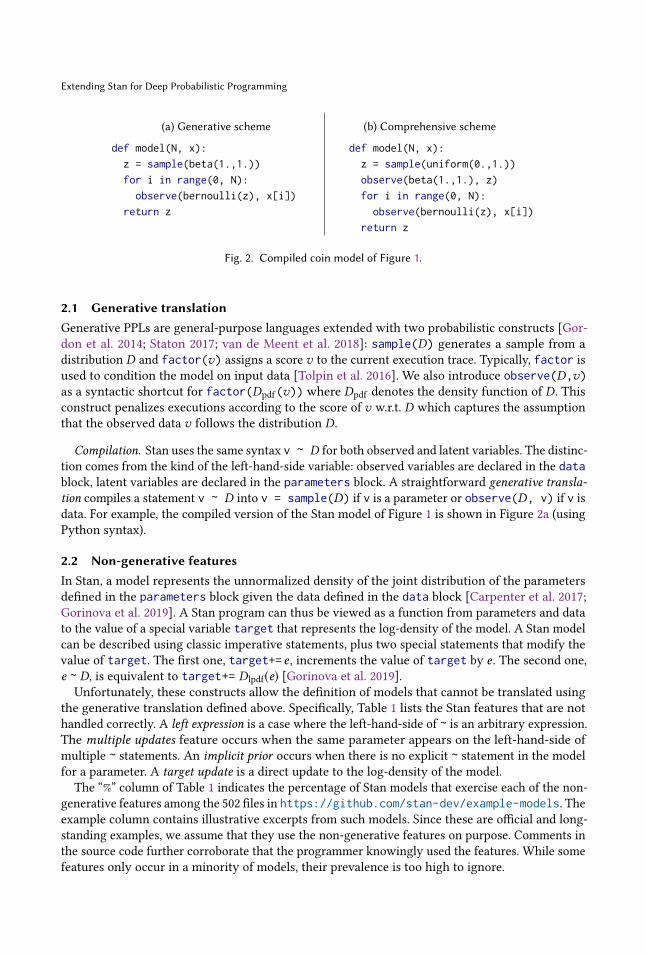
(a) Generative scheme

def model(N, x):

z = sample(beta(1.,1.))

for i in range(0, N):

observe(bernoulli(z), x[i])

return z

(b) Comprehensive scheme

def model(N, x):

z = sample(uniform(0.,1.))

observe(beta(1.,1.), z)

for i in range(0, N):

observe(bernoulli(z), x[i])

return z

Fig. 2. Compiled coin model of Figure 1.

2.1 Generative translationGenerative PPLs are general-purpose languages extended with two probabilistic constructs [Gor-

don et al. 2014; Staton 2017; van de Meent et al. 2018]: sample(D) generates a sample from a

distribution D and factor(v) assigns a score v to the current execution trace. Typically, factor is

used to condition the model on input data [Tolpin et al. 2016]. We also introduce observe(D,v)as a syntactic shortcut for factor(Dpdf(v)) where Dpdf denotes the density function of D. Thisconstruct penalizes executions according to the score of v w.r.t. D which captures the assumption

that the observed data v follows the distribution D.

Compilation. Stan uses the same syntax v ~ D for both observed and latent variables. The distinc-

tion comes from the kind of the left-hand-side variable: observed variables are declared in the datablock, latent variables are declared in the parameters block. A straightforward generative transla-tion compiles a statement v ~ D into v = sample(D) if v is a parameter or observe(D, v) if v isdata. For example, the compiled version of the Stan model of Figure 1 is shown in Figure 2a (using

Python syntax).

2.2 Non-generative featuresIn Stan, a model represents the unnormalized density of the joint distribution of the parameters

defined in the parameters block given the data defined in the data block [Carpenter et al. 2017;

Gorinova et al. 2019]. A Stan program can thus be viewed as a function from parameters and data

to the value of a special variable target that represents the log-density of the model. A Stan model

can be described using classic imperative statements, plus two special statements that modify the

value of target. The first one, target+= e , increments the value of target by e . The second one,

e ~ D, is equivalent to target+= Dlpdf(e) [Gorinova et al. 2019].Unfortunately, these constructs allow the definition of models that cannot be translated using

the generative translation defined above. Specifically, Table 1 lists the Stan features that are not

handled correctly. A left expression is a case where the left-hand-side of ~ is an arbitrary expression.

The multiple updates feature occurs when the same parameter appears on the left-hand-side of

multiple ~ statements. An implicit prior occurs when there is no explicit ~ statement in the model

for a parameter. A target update is a direct update to the log-density of the model.

The “%” column of Table 1 indicates the percentage of Stan models that exercise each of the non-

generative features among the 502 files in https://github.com/stan-dev/example-models. Theexample column contains illustrative excerpts from such models. Since these are official and long-

standing examples, we assume that they use the non-generative features on purpose. Comments in

the source code further corroborate that the programmer knowingly used the features. While some

features only occur in a minority of models, their prevalence is too high to ignore.

https://github.com/stan-dev/example-models


Table 1. Stan features: example, prevalence and compilation.

Feature % Example Compilation

Left expression 7.7 sum(phi) ~ normal(0, 0.001*N); observe(Normal(0.,0.001*N), sum(phi))

Multiple updates 3.9

phi_y ~ normal(0,sigma_py);phi_y ~ normal(0,sigma_pt)

observe(Normal(0.,sigma_py), phi_y);observe(Normal(0.,sigma_pt), phi_y)

Implicit prior 60.7

real alpha0;/* missing 'alpha0 ~ ...' */

alpha0 = sample(ImproperUniform())

Target update 16.3

target += -0.5 * dot_self(phi[node1] - phi[node2]);

factor(-0.5 * dot_self(phi[node1] - phi[node2])))

2.3 Comprehensive translationThe previous section illustrates that Stan is centered around the definition of target, not aroundgenerating samples for parameters, which is required by generative PPLs. The idea of the com-

prehensive translation is to add an initialization step to generate samples for all the parameters

and compile all Stan ~ statements as observations. To initialize the parameters we draw from the

uniform distribution in the definition domain of the parameters. For the biased coin example, the

result of this translation is shown in Figure 2b: The parameter z is first sampled uniformly on its

definition domain and then conditioned with an observation.

The compilation column of Table 1 illustrates the translation of non-generative features. Left

expression and multiple updates are simply compiled into observations. Parameter initialization

uses the uniform distribution over its definition domain. For unbounded domains, we introduce

new distributions (e.g., ImproperUniform) with a constant density that can be normalized away

during inference. The target update is compiled into a factor which increases the log-probability

of the execution by the given number. The complete compilation scheme is detailed in Section 3.3.

Intuition of the correctness. The semantics of Stan as described in [Gorinova et al. 2019] is the

semantics of a classical imperative language that defines an environment containing, in particular,

the value of the special variable target: the unnormalized log-density of the model. On the other

hand, the semantics of a generative PPL as described in [Staton 2017] defines a kernel mapping an

environment to a measurable function. Our compilation scheme adds uniform initializations for all

parameters which comes down to the Lebesgue measure on the parameters space, and translates all

~ statements to observe statements. We can then show that a succession of observe statements

yields a distribution with the same log-density as the Stan semantics. The correctness proof is

detailed in Section 3.4.

2.4 ImplementationThe comprehensive compilation scheme can be used to compile any Stan program to a generative

PPL leveraging the rich set of existing Stan models for testing and benchmarking. As a proof

of concept, we implemented a compiler from Stan to Pyro [Bingham et al. 2019], a probabilistic

programming language in the line of WebPPL.

Vectorization. Compiling Stan to Pyro also raises the problem of automatic vectorization. In

Stan, expressions are automatically vectorized. For instance, the statement z ~ normal(0, 1)automatically lifts the scalars 0 and 1 to the shape of z. To generate correct Pyro code, we need to

explicitly lift these constants: z = sample(normal(zeros(s), ones(s))) where s is the shapeof z, and the functions zeros and ones return arrays of zeros and ones, respectively. We thus

extend the Stan type system to infer dimensions and sizes (Section 4). Our type system allows the

programmer to omit redundant dimensions, leaving them to the compiler to deduce.


Extensions. Pyro is a deep universal probabilistic programming language with native support

for variational inference, and we can thus can leverage the deep features of the language back to

Stan (Section 5). Our Stan extension — DeepStan — thus support explicit variational guides (Sec-

tion 5.1) and deep neural networks to capture complex relations between parameters (Section 5.2).

3 SEMANTICS AND COMPILATIONThis section, building on previous work, first formally defines the semantics of Stan (Section 3.1)

and the semantics of GProb, a small generative probabilistic language (Section 3.2). It then defines

the compilation function from Stan to GProb (Section 3.3) and proves its correctness (Section 3.4).

3.1 Stan: a Declarative Probabilistic LanguageThe Stan language is informally described in [Carpenter et al. 2017]. A Stan program is a sequence

of blocks in the following order, where the only mandatory block is model. Variables declared in

one block are visible in subsequent blocks.

program ::= functions {fundecl∗} ? function declarations

data {decl∗} ? variable names of the input data

transformed data {decl∗ stmt} ? data pre-processing

parameters {decl∗} ? variable names of the parameters

transformed parameters {decl∗ stmt} ? pre-processing of the parameters

model {decl∗ stmt} body of the model

generated quantities {decl∗ stmt} ? post-processing of the parameters

Variable declarations (decl∗) are lists of variables names with their types (e.g., int N;) or arrayswith their type and shape (e.g., real x[N]). Types can be constrained to specify the domain of a

variable (e.g., real <lower=0> x for x ∈ R+). Note that vector and matrix are primitive types

that can be used in arrays (e.g. vector[N] x[10] is an array of 10 vectors of size N). Shapes andsizes of arrays, matrices, and vectors are explicit and can be arbitrary expressions.

decl ::= base_type constraint x ; | base_type constraint x [shape] ;

base_type ::= real | int | vector[size] | matrix[size,size]constraint ::= ε | < lower = e , upper = e > | < lower = e > | < upper = e >

shape ::= size | shape , sizesize ::= e

Inside a block, Stan is similar to a classic imperative language, with the addition of two specialized

statements: target += e directly updates the log-density of themodel (stored in the reserved variable

target), and x ~ D indicates that a variable x follows a distribution D.

stmt ::= x = e variable assignment

| x[e1,...,en] = e array assignment

| stmt1; stmt2 sequence

| for (x in e1:e2) {stmt} loop over a range

| for (x in e) {stmt} loop over the elements of a collection

| while (e) {stmt} while loop

| if (e) stmt1 else stmt2 conditional

| skip no operation

| target += e direct update of the log-density

| e ~ f (e1,...,en) probability distribution


Expressions comprise constants, variables, arrays, vectors, matrices, access to elements of an

indexed structure, and function calls (also used to model binary operators):

e ::= c | x | {e1,...,en} | [e1,...,en] | [[e11,...,e1m],...,[en1,...,enm]] | e1[e2] | f (e1,...,en)

Semantics. The evaluation of a Stan program comprises three steps:

(1) data preparation with data and transformed data(2) inference over the model defined by parameters, transformed parameters, and model(3) post-processing with generated quantities

Section 3.3 shows how to efficiently compile the pre- and post-processing blocks, but in terms of

semantics, any Stan program can be rewritten into an equivalent program with only the three

blocks data, parameters, and model.

functions {fundecls}data {declsd} data {declsd}transformed data {declstd stmttd} parameters {declsp}parameters {declsp} ≡ model {transformed parameters {declstp stmttp} declstd declstp declsm declsдmodel {declsm stmtm} stmt ′td stmt ′tp stmt ′m stmt ′дgenerated quantities {declsд stmtд} }

Functions declared in functions have been inlined. To simplify the presentation of the semantics,

we focus in the following on this simplified language.

Notations. To refer to the different parts of a program, we will use the following functions. For a

Stan program p = data {declsd} parameters {declsp} model {declsm stmt}:

data(p) = declsdparams(p) = declspmodel(p) = stmt

In the following, an environment γ : Var → Val is a mapping from variables to values, γ (x)returns the value of the variable x in an environment γ , γ [x ← v] returns the environment γ where

the value of x is set to v , and γ1,γ2 denotes the union of two environments.

We note

∫X µ(dx)f (x) the integral of f w.r.t. the measure µ where x ∈ X is the integration

variable. When µ is the Lebesgue measure we also write

∫X f (x)dx .

Following [Gorinova et al. 2018], we define the semantics of the model block as a deterministic

function that takes an initial environment containing the input data and the parameters, and returns

an updated environment where the value of the variable target is the un-normalized log-density

of the model.

We can then define the semantics of a Stan program as a kernel [Kozen 1981; Staton 2017; Staton

et al. 2016], that is, a function {[p]} : D → ΣX → [0,∞] where ΣX denotes the σ -algebra of theparameter domain X , that is, the set of measurable sets of the product space of parameter values.

Given an environment D containing the input data, JpKD is a measure that maps a measurable

set of parameter values U to a score in [0,∞] obtained by integrating the density of the model,

exp(target), over all the possible parameter values inU .

{[p]}D = λU .

∫Uexp(Jmodel(p)KD,θ (target)) dθ


Jx = eKγ = γ [x ← JeKγ ]Jx[e1,...,en] = eKγ = γ [x ← (x[Je1Kγ ,..., JenKγ ]← JeKγ )]Js1; s2Kγ = Js2KJs1Kγ

Jfor (x in e1:e2) {s}Kγ = let n1 = Je1Kγ in let n2 = Je2Kγ inif n1 > n2 then γelse Jfor (x in n1 + 1:n2) {s}KJsKγ [x←n

1]

Jwhile (e) {s}Kγ = if JeKγ = 0 then γelse Jwhile (e) {s}KJsKγ

Jif (e) s1 else s2Kγ = if Je1Kγ , 0 then Js1Kγ else Js2KγJskipKγ = γ

Jtarget += eKγ = γ [target← γ (target) + JeKγ ]Je1 ~ e2Kγ = let D = Je2Kγ in

qtarget += Dlpdf (e1)

yγ

Fig. 3. Semantics of statements

Given the input data, the posterior distribution of a Stan program is then obtained by normalizing

the measure {[p]}D . In practice, the integrals are often untractable, and the runtime relies on

approximate inference schemes to compute the posterior distribution.

We now detail the semantics of statements and expressions that can be used in the model block.

This formalization is similar to the semantics proposed in [Gorinova et al. 2018] but expressed in a

denotational style.

Statements. The semantics of a statement JsK : (Var → Val) → (Var → Val) is a function from

an environment γ to an updated environment. Figure 3 gives the semantics of Stan statements.

The initial environment always contains the the reserved variable target initialized to 0. Anassignment updates the value of a variable or of a cell of an indexed structure in the environment. A

sequence s1; s2 evaluates s2 in the environment produced by s1. A for loop on ranges first evaluates

the value of the bounds n1 and n2 and then repeats the execution of the body 1 + n2 − n1 times.

Iterations over indexed structures depend on the underlying type. For vectors and arrays, iteration

is limited to one dimension (i is a fresh variable name):

Jfor (x in e) {s}Kγ = letv = JeKγ inJfor (i in 1:length(v)) {x = v[i]; s}Kγ

For matrices, iteration is over the two dimensions (i and j are fresh variable names):

Jfor (x in e) {s}Kγ = letv = JeKγ insfor (i in 1:length(v))

for (j in 1:length(v[i][j])) {x = v[i][j]; s}

{

γ

A while loop repeats the execution of its body while the condition is not 0. A if statement executes

one of the two branches depending on the value of the condition. A skip leaves the environment

unchanged. A statement target += e adds the value of e to target in the environment. Finally,

a statement e1 ~ e2 evaluates the expression e2 into a probability distribution D and updates the

target with the value of the log-density of D at e1.


JcKγ = c J{e1,...,en}Kγ = {Je1Kγ ,..., JenKγ }

JxKγ = γ (x) J[e1,...,en]Kγ = [Je1Kγ ,..., JenKγ ]

Je1[e2]Kγ = Je1Kγ [Je2Kγ ] Jf (e)Kγ = f (JeKγ )

Fig. 4. Semantics of expressions

Expressions. The semantics of an expression JeK : (Var → Val) → Val is a function from a

environment to values. Figure 4 gives the semantics of Stan expressions. The value of a constant is

itself. The value of a variable is the corresponding value stored in the environment. The value of an

array, a vector, or a matrix is obtained by evaluating all its components. Accessing a component

of an indexed structure looks up the corresponding value in the associated data. A function call

applies the function to the value of the arguments. Functions are limited to built-in operations

like + or normal (user defined functions have been inlined).

3.2 GProb: a Simple Generative Probabilistic LanguageTo formalize the compilation, we first define the target language: GProb, a simple generative

probabilistic language similar to the one defined in [Staton 2017]. GProb is an expression language

with the following syntax:

e ::= c | x | {e1,...,en} | [e1,...,en] | e1[e2] | f (e1,...,en)| letx = e1 in e2 | letx[e1,...,en] = e in e ′

| if (e) e1 else e2 | forX (x in e1:e2) e3 | whileX (e1) e2| factor(e) | sample(e) | return(e)

An expression is either a Stan expression, a local binding (let), a conditional (if), or a loop (for or

while). To simplify the presentation, loops are parameterized by the set X of variables that are

updated in their body. GProb also contains the classic probabilistic expressions: sample draws asample from a distribution, and factor assigns a score to the current execution trace to condition

the model. The return expression is used to lift a deterministic expression to a probabilistic context.

We also introduce observe(D,v) as a syntactic shortcut for factor(Dpdf(v)) where Dpdf

denotes the density function ofD. This construct penalizes the current execution with the likelihoodof v w.r.t. D which captures the assumption that the observed data v follows the distribution D.

Semantics. Following [Staton 2017] we give a measure-based semantics to GProb. The semantics

of an expression is a kernel which, given an environments, returns a measure on the set of possible

values. Again, given the input data, the posterior distribution of a GProb program is then obtained

by normalizing the corresponding measure.

The semantics of GProb is given in Figure 5. A deterministic expression is lifted to a probabilistic

expression with the Dirac delta measure (δx (U ) = 1 if x ∈ U , 0 otherwise). A local definition

letx = e1 in e2 is interpreted by integrating the semantics of e2 over the set of all possible valuesfor x . In the following, we use the more concise union notation γ ,x to bind the value of x in the

environment γ in the integrals. The semantics of a local definition can thus be rewritten:

{[letx = e1 in e2]}γ = λU .

∫X{[e1]}γ (dx) × {[e2]}γ ,x (U )

Compared to the language defined in [Staton 2017], we added Stan loops. Loops behave like a

sequence of expressions and return the values of the variables updated by their body. Consider, for

example, the whileX (e1) e2 expression. First, the condition is evaluated. If the loop terminates,

we return the measure corresponding to the variables X updated by the loop. Otherwise, similarly


{[return(e)]}γ = λU . δJeKγ (U )

{[letx = e1 in e2]}γ = λU .

∫X{[e1]}γ (dv) × {[e2]}γ [x←v](U )

{[letx[e1,...,en] = e in e ′]}γ = λU .

∫X{[e]}γ (dv) × {[e ′]}γ [x←(x[Je1Kγ ,...,JenKγ ]←v)](U )

{[forX (x in e1:e2) e3]}γ = λU .let n1 = Je1Kγ in let n2 = Je2Kγ in

if n1 > n2 then δγ (X)(U )

else∫X{[e3]}γ [x←n1](dX) × {[forX (x in n1 + 1:n2) e3]}γ ,X(U )

{[whileX (e1) e2]}γ = λU .if Je1Kγ = 0 then δγ (X)(U )

else∫X{[e2]}γ (dX) × {[whileX (e1) e2]}γ ,X(U )

{[if (e) e1 else e2]}γ = λU .if JeK , 0 then {[e1]}γ (U ) else {[e2]}γ (U )

{[sample(e)]}γ = λU . JeKγ (U )

{[factor(e)]}γ = λU . exp(JeKγ )

Fig. 5. Generative probabilistic language semantics

to the local binding, we integrates the next iteration of the loop over the set of all possible values

for the set of variables X.The semantics of probabilistic operators is the following. The semantics of sample(e) is the

probability distribution JeKγ (e.g.N(0, 1)). A type system omitted here for conciseness ensures that

we only sample from distributions. The semantics of factor(e) is the constant measure whose

value is exp(JeK) (this operator corresponds to score in [Staton 2017] but in log-scale, which is

common for numerical precision).

3.3 Comprehensive TranslationThe key idea of the comprehensive translation is to first sample all parameters from priors with a

constant density that can be normalized away during inference (e.g., Uniform on bounded domains),

and then compile all ~ statements into observe statements.

The compilation functions for the parameters Pk (params(p)) and the model Sk (model(p)) areboth parameterized by a continuation k . The compilation of the entire program first compiles the

parameters to introduce the priors, then compiles the model, and finally adds a return statement

for all the parameters. In continuation passing style:

C(p) = PSreturn(params(p))(model(p)) (params(p))

Parameters. In Stan, parameters can only be real, array of reals, vectors, or matrices, and are

thus defined on Rn with optional domain constraints (e.g. <lower=0>). For each parameter, the

prior is either the Uniform distribution on a bounded domain, or an improper prior with a constant

density w.r.t. the Lebesgue measure that we call ImproperUniform. The compilation function of the

parameters, defined Figure 6, thus produces a succession of sample expressions:

Pk (params(p)) = letx1 = D1 in . . . letxn = Dn in k

where for each parameter xi , Di is either Uniform or ImproperUniform.


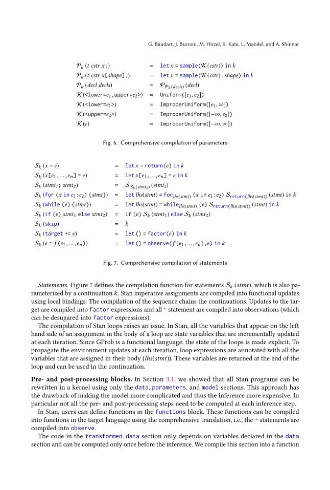
Pk (t cstr x;) = letx = sample(K (cstr)) in kPk (t cstr x[shape];) = letx = sample(K (cstr) ,shape) in k

Pk (decl decls) = PPk (decls) (decl)K (<lower=e1,upper=e2>) = Uniform([e1, e2])K (<lower=e1>) = ImproperUniform([e1,∞])K (<upper=e2>) = ImproperUniform([−∞, e2])K (ε) = ImproperUniform([−∞,∞])

Fig. 6. Comprehensive compilation of parameters

Sk (x = e) = letx = return(e) in k

Sk (x[e1,...,en] = e) = letx[e1,...,en] = e in k

Sk (stmt1; stmt2) = SSk (stmt2) (stmt1)Sk (for (x in e1:e2) {stmt}) = let lhs(stmt) = forlhs(stmt) (x in e1:e2) Sreturn(lhs(stmt)) (stmt) in kSk (while (e) {stmt}) = let lhs(stmt) = whilelhs(stmt) (e) Sreturn(lhs(stmt)) (stmt) in kSk (if (e) stmt1 else stmt2) = if (e) Sk (stmt1) else Sk (stmt2)Sk (skip) = k

Sk (target += e) = let () = factor(e) in k

Sk (e ~ f (e1,...,en)) = let () = observe(f (e1,...,en),e) in k

Fig. 7. Comprehensive compilation of statements

Statements. Figure 7 defines the compilation function for statements Sk (stmt), which is also pa-

rameterized by a continuation k . Stan imperative assignments are compiled into functional updates

using local bindings. The compilation of the sequence chains the continuations. Updates to the tar-

get are compiled into factor expressions and all ~ statement are compiled into observations (which

can be desugared into factor expressions).The compilation of Stan loops raises an issue. In Stan, all the variables that appear on the left

hand side of an assignment in the body of a loop are state variables that are incrementally updated

at each iteration. Since GProb is a functional language, the state of the loops is made explicit. To

propagate the environment updates at each iteration, loop expressions are annotated with all the

variables that are assigned in their body (lhs(stmt)). These variables are returned at the end of the

loop and can be used in the continuation.

Pre- and post-processing blocks. In Section 3.1, we showed that all Stan programs can be

rewritten in a kernel using only the data, parameters, and model sections. This approach has

the drawback of making the model more complicated and thus the inference more expensive. In

particular not all the pre- and post-processing steps need to be computed at each inference step.

In Stan, users can define functions in the functions block. These functions can be compiled

into functions in the target language using the comprehensive translation, i.e., the ~ statements are

compiled into observe.The code in the transformed data section only depends on variables declared in the data

section and can be computed only once before the inference. We compile this section into a function


that takes as argument the data and returns the transformed data. The variables declared in the

transformed data section become new inputs for the model.

On the other hand, the code of the transformed parameters block must be part of the model

since it depends on the model parameters. This section is thus inlined in the compiled model.

Finally, the generated quantities block can be executed only once on the result of the in-

ference. We compile this section into a function of the data, transformed data, and parameters

returned by the model. Since a generated quantity may depend on transformed parameters, the

code of the transformed parameters block must also be inlined in this function to be usable.

Compiling to Pyro. In Pyro, the probabilistic operator are v = sample(name,D) (sample) andsample(name,D,obs=e) (observe). Note that, in both cases, the user must provide a unique namefor the internal Pyro namespace.

Translating target update requires overcoming the obstacle that Pyro does not directly expose

the log-density accumulator to the programmer. Instead, we use the exponential distribution with

parameter λ = 1 whose density function is Exppdf(1)(x) = e−x . Observing a value −v from this

distribution multiplies the score by ev , which corresponds to the update target += v . This approachis similar to the “zeros trick” from BUGS [Lunn et al. 2012].

Finally, in Stan, expressions can be automatically vectorized, but in Pyro, array dimensions must

be explicit. Section 4 introduces a type system to deduce the size and shape of Stan vectorized

constructs to enable the compiler to make them explicit.

3.4 Correctness of the CompilationWe can now show that a Stan program and the corresponding compiled code yield the same

un-normalized measure up to a constant factor (and thus the same posterior distribution). The

proof comprises two steps: (1) we simplify the sequence of sample statements introduced by the

compilation of the parameters, and (2) we show that the value of the Stan target corresponds tothe score computed by the generated code.

Priors. First, we show that the nested integrals introduced by the sequence of sample statements

for the parameters priors can be simplified into a single integral over the parameter domain.

Lemma 3.1. For all Stan program p, and environment γ :

{[C(p)]}γ = λU .

∫U{[Sreturn(()) (model(p))]}γ ,θ ({()})dθ

Proof. In the following declsp = params(p) and stmt = model(p). By definition of the compila-

tion function, C(p) has the following shape:letx1 = D1 in . . . letxn = Dn in Sreturn(declsp) (stmt)

where for each parameter xi , Di is either Uniform or ImproperUniform. In both cases the corre-

sponding density is constant w.r.t. the Lebesgue measure on its domain. Since the kernels defined

by GProb expressions are always s-finite [Staton 2017], from the semantics of GProb (Section 3.2)

and the Fubini-Tonelli theorem, we have:

{[C(p)]}γ = {[Sreturn(declsp) (p)]}γ

= λU .

∫X1

D1(dx1)· · ·∫Xn

Dn (dxn ){[Sreturn(declsp) (stmt)]}γ , {x1, ...,xn }(U )

∝ λU .

∫X1

· · ·∫Xn

{[Sreturn(declsp) (stmt)]}γ , {x1, ...,xn }(U ) dx1 . . .dxn

= λU .

∫X=X1×···×Xn

{[Sreturn(declsp) (stmt)]}γ ,θ (U ) dθ


In Stan, parameters declared in declsp cannot appear in the left-hand side of an assignment, which

means that the evaluation of the model statements stmt cannot update the value of the parameters.

The evaluation of {[Sreturn(declsp) (stmt)]}γ ,θ (U ) thus leaves θ unchanged and terminates with

{[return(declsp)]}γ ′,θ (U ) which is equal to {[return(declsp)]}θ (U ). We can thus decompose the

evaluation of compiled code as follows:

{[Sreturn(declsp) (stmt)]}γ ,θ (U ) =∫X{[Sreturn(()) (stmt)]}γ ,θ (dx) × {[return(declsp)]}θ (U )

= {[Sreturn(()) (stmt)]}γ ,θ ({()}) × δθ (U )

Going back to the previous equation, we now have

{[C(p)]}γ = λU .

∫X{[Sreturn(()) (stmt)]}γ ,θ ({()}) × δθ (U ) dθ

= λU .

∫U{[Sreturn(()) (stmt)]}γ ,θ ({()}) dθ

□

Score and target. We now show that the value of the Stan target variable corresponds to the

score computed by the generated code.

Lemma 3.2. For all Stan statements stmt compiled with a continuation k , if γ (target) = 0, andJstmtKγ = γ

′,{[Sk (stmt)]}γ = λU . exp(γ ′(target)) × {[k]}γ ′[target←0](U )

Proof. The proof is done by induction on the structure of stmt using the definition of the

compilation function (Section 3.3) and the semantics of GProb. We now detail just a few key cases.

Assignment. The evaluation of x = e does not update the value of target and its initial value is 0

by hypothesis. With γ ′ = Jx = eKγ we have γ ′[target← 0] = γ ′ and exp(γ ′(target)) = 1. Then

from the semantics of GProb we have:

{[Sk (x = e)]}γ = {[letx = return(e) in k]}γ

= λU .

∫X{[return(e)]}γ (dv) × {[k]}γ [x←v](U )

= λU .

∫XδJeKγ (dv) × {[k]}γ [x←v](U )

= λU .1 × {[k]}γ [x←JeKγ ](U )

= λU .1 × {[k]}Jx = eKγ (U )

Target update. Since the evaluation of target += e only updates the value of target and its

initial value is 0, with γ ′ = Jtarget += eKγ we have γ = γ ′[target← 0], and γ ′(target) = JeKγ .Then from the semantics of GProb we have:

{[Sk (target += e)]}γ = {[let () = factor(e) in k]}γ

= λU .

∫X{[return(e)]}γ (dv) × {[k]}γ (U )

= λU .

∫Xexp(JeKγ )(dv) × {[k]}γ (U )

= λU . exp(JeKγ ) × {[k]}γ (U )


Sequence. From the induction hypothesis and the semantics of GProb we have with γ1 = Jstmt1Kγand γ2 = Jstmt2Kγ1[target←0]:

{[Sk (stmt1; stmt2)]}γ = {[SSk (stmt2) (stmt1)]}γ= λU .exp(γ1(target)) × {[Sk (stmt2)]}γ1[target←0](U )= λU .exp(γ1(target)) × exp(γ2(target)) × {[k]}γ2[target←0](U )= λU .exp(γ1(target) + γ2(target)) × {[k]}γ2[target←0](U )

On the other hand, from the semantics of Stan (Section 3.1), for any real value t we have:

JstmtKγ [target←t ] (target) = t + JstmtKγ [target←0] (target)

Therefore: Jstmt1; stmt2Kγ (target) = γ1(target) + γ2(target) which conclude the proof. □

Correctness.We now have all the elements to prove that the comprehensive compilation is correct.

That is, generated code yield the same un-normalized measure up to a constant factor that will be

normalized away by the inference.

Theorem 3.3. For all Stan programs p, the semantics of the source program is equal to the semanticsof the compiled program up to a constant:

{[p]}D ∝ {[C(p)]}DProof. The proof is a direct consequence of Lemmas 3.1 and 3.2 and the definition of the two

semantics.

{[C(p)]}D ∝ λU .

∫U{[Sreturn(()) (model(p))]}D,θ ({()}) dθ

= λU .

∫Uexp(Jmodel(p)KD,θ (target)) × {[return(())]}({()}) dθ

= λU .

∫Uexp(Jmodel(p)KD,θ (target)) dθ

= {[p]}D□

4 VECTORIZATIONVectorization is a style of programming where operations are applied to entire tensors (i.e, arrays,

vectors, or matrices) instead of individual elements. For example, in Stan, z ~ normal(0,1) liftsthe scalars 0 and 1 to the shape of z. Vectorization is both convenient (briefer code) and efficient

(faster on vector units). Unfortunately, while the Stan compiler gets away with keeping shapes

and sizes implicit during compilation, our compiler to Pyro must make them explicit to generate

correct code. Thus, it needs a tensor shape analysis, described in this section. Explicit knowledge

of shapes and sizes also enables our compiler to check if types are correct and if not, report errors

earlier than the Stan compiler would.

Sizes of tensor variables can depend on each other, as in the code

real encoded[2,nz] = encoder(x); real mu_z[nz] = encoded[1];Due to the assignment, mu_z must have the same size nz as the second dimension of encoded.Given that it can be deduced, some users may prefer not to explicitly specify it by hand, as in

real encoded[2,nz] = encoder(x); real mu_z[_] = encoded[1];


t ≡ t

t2 ≡ t1t1 ≡ t2

t1 ≡ t2 n1 ≡ n2t1[n1] ≡ t2[n2]

n1 ≡ n2row_vector[n1] ≡ row_vector[n2]

t1 ≡ t2 n1,...,nk ≡ d

t1[n1]...[nk] ≡ t2[]dn1 ≡ n2

vector[n1] ≡ vector[n2]

n1 ≡ n2 m1 ≡m2

matrix[n1,m1] ≡ matrix[n2,m2]

Fig. 8. Type equivalence: t1 ≡ t2 means t1 is equivalent to (unifies with) t2.

This ability to keep some sizes implicit in the source code is another benefit of having a tensor

shape analysis. While it is only a minor convenience in the above example, when used with our

DeepStan extension to Stan, it becomes a major convenience. This is because neural network shapes

are specified in PyTorch, and forcing users to redundantly specify them in DeepStan code would be

brittle and cause clutter. Instead, DeepStan supports declarations such as real mlp.l1.weight[*];where * leaves not only sizes but even the number of dimensions to be deduced by the compiler.

The tensor shape analysis must support polymorphism both over sizes of individual dimensions

and over the number of dimensions. Furthermore, it must handle Stan’s standard library of size-

polymorphic functions and distributions (conceptually, our compiler desugars infix operators such

as + into binary function invocations). Another factor that complicates the analysis is target-typing:

the vectorization of a function or distribution is determined not just by its actual arguments but

also by how the result gets used. Finally, the tensor shape analysis must handle Stan’s assortment

of tensor types including vectors, arrays, matrices, and row vectors.

Our solution is a Hindley-Milner style analysis that conceptually comprises the following steps:

(1) Give a type to each variable and expression in the program, emitting type errors as needed,

while also gathering constraints for types that are not fully determined yet.

(2) Use unification on the constraints to determine more concrete types, again emitting type

errors as needed when attempting to unify incompatible types.

(3) If some types are still ambiguous (i.e., the information is not available at startup, as opposed

to constants or information that can be read from data or neural networks), emit warnings.

(4) Use the deduced sizes in code generation, for instance, to properly initialize tensors.

The tensor shape analysis internally uses a more expressive set of types than the surface types

used by the programmer. They are defined as follows:

type ::= base_type | type[size] | type[]dimbase_type ::= real | int | vector[size] | matrix[size,size]size ::= e | σdim ::= shape | δ | shape(e)shape ::= size | shape,sizefunc ::= typevect ∗ · · · ∗ typevect → type | typevect ∗ · · · ∗ typevect → funcvect ::= true | falseschema ::= ∀σ1, ...,σk ,∀δ1, ...,δm .func

Non-terminal base_type is the same as in the surface grammar from Section 3.1. We introduce poly-

morphic size variables (σ ) that have to be deduced by the compiler. For example, matrix[42,_] x;yields the type matrix[42,σ]. Also, there is a new type t[]dim representing an array of elements of

type t with a dimension specified by dim. Dimensions can be specified by the size of each dimension,

a polymorphic shape variable (δ ), or they can have the same shape as the result of an expression

evaluation. For example, int x[*]; yields the type int[]δ . There are two kinds of func type,


H ⊢ c : t

H ⊢ e : int

H ⊢ e : real

H (x) = t

H ⊢ x : t

H ⊢ ei : ti ti ≡ t

H ⊢ {e1,...,en} : t[n]

H ⊢ ei : real

H ⊢ [e1,...,en] : vector[n]

H ⊢ ei j : real

H ⊢ [[e11,...,e1m ],...,[en1,...,enm ]] : matrix[n,m]

H ⊢ e1 : t[n] H ⊢ e2 : int

H ⊢ e1[e2] : t

H ⊢ e1 : vector[n] H ⊢ e2 : int

H ⊢ e1[e2] : real

H ⊢ e1 : row_vector[n] H ⊢ e2 : int

H ⊢ e1[e2] : real

H ⊢ e1 : matrix[n1,n2] H ⊢ e2 : int

H ⊢ e1[e2] : row_vector[n2]

tv1

1∗ ... ∗ tvnn → t ∈ inst(f ) H ⊢ ei : t ′i ti ⇑vi t ′i

H ⊢ f (e1,...,en) : t

Fig. 9. Typing of expressions: H ⊢ e : t means that in typing environment H , expression e has type t .

t ⇑v t t[n] ⇑true t vector[n] ⇑true real row_vector[n] ⇑true real

vector[n][m] ⇑true vector[n] vector[n][m] ⇑true row_vector[n]

row_vector[n][m] ⇑true row_vector[n] row_vector[n][m] ⇑true vector[n]

Fig. 10. Vectorization relation t ⇑v t ′ means that if v is true then t is a vectorized form of t ′.

corresponding to regular functions and higher-order functions with vect annotations indicatingwhich arguments can or cannot be implicitly vectorized. Finally, schema imbues functions with

size and shape polymorphism.

Figure 8 presents type equivalence rules. These represent type constraints gathered from typing

rules to be resolved later during unification. Equivalence is reflexive and symmetric. For structured

types (arrays, vectors, etc.), type constraints imply corresponding size and shape constraints. For

example, vector[N] ≡ vector[10] adds the constraint that N must be equal to 10 and int[]δ ≡int[50][50] adds the constraint that δ must be a two dimensional array of size 50.

Figure 9 presents type rules for expressions. A typing environment H is a map from names to

internal types. Constants c type-check against their intrinsic type. Type int is a subtype of real.A use of a name x type-checks against its declared type in H . Arrays, vectors, and matrices that

are constructed from literals have concrete sizes. Indexing requires integer subscripts and returns

element types. Due to vectorization, the rule for function call expressions is the most intricate. The

set inst(f ) represents instantiations of the type of the function f with vectorization information vfor each argument. Each vi indicates whether the corresponding argument ei can be lifted to an

array. Vectorization must infer the sizes of arrays.

Figure 10 presents the vectorization relation t ⇑v t ′. Ifv is true, then t is a composite type derived

by appropriate replication of values of t ′ to yield components of t . If v is false, then only the trivial

vectorization where t and t ′ are the same works, i.e., there is no broadcasting. For example, if x is

of type real[10] in H , then we have the following typing derivation:

real[10]true ∗ real[10]true → real[10] ∈ inst(∀σ .real[σ]true ∗ real[σ]true → real[σ])H ⊢ x : real[10] H ⊢ 1 : real real[10] ⇑true real

H ⊢ normal(x, 1) : real[10]


H (x) = t1 H ⊢ e : t2 t1 ≡ t2H ⊢ x = e

H ⊢ stmt1 H ⊢ stmt2

H ⊢ stmt1; stmt2

H ⊢ e : real

H ⊢ target += e

H (x) = t1[n1]...[nk] H ⊢ ei : int H ⊢ e : t2 t1 ≡ t2H ⊢ x[e1,...,ek] = e

H (x) = vector[n] H ⊢ e1 : int H ⊢ e : real

H ⊢ x[e1] = e

H (x) = row_vector[n] H ⊢ e1 : int H ⊢ e : real

H ⊢ x[e1] = e

H (x) = matrix[n,m] H ⊢ e1 : int H ⊢ e2 : int H ⊢ e : real

H ⊢ x[e1,e2] = e

H ⊢ e1 : int H ⊢ e2 : int H + [x : int] ⊢ stmt

H ⊢ for (x in e1:e2) {stmt}

H ⊢ e : t[n] H + [x : t] ⊢ stmt

H ⊢ for (x in e) {stmt}

H ⊢ e : vector[n] H + [x : real] ⊢ stmt


H ⊢ e : matrix[n1,n2] H + [x : real] ⊢ stmt


H ⊢ e : real H ⊢ stmt

H ⊢ while (e) {stmt}

H ⊢ e : real H ⊢ stmt1 H ⊢ stmt2

H ⊢ if (e) stmt1 else stmt2 H ⊢ skip

tv1

1∗ ... ∗ tvnn → tv → real ∈ inst(flpdf ) H ⊢ e : t H ⊢ ei : t ′i ti ⇑vi t ′i

H ⊢ e ~ f (e1,...,en)

Fig. 11. Typing of statements: H ⊢ stmt means in typing environment H , statement stmt is well-typed.

Figure 11 presents type rules for statements. Assignments introduce type equivalence constraints.

Indexing requires integer subscripts. Loops with for introduce new local bindings into the type

environment via the H + binding notation (in Stan all variables name must be unique). Due to

vectorization, the rule for ~ statements is the most intricate. A distribution f : t1 ∗ ... ∗ tn →t → real is treated as a higher-order function where t1 ∗ ... ∗ tn is the type of the parameters

(e.g., (0,1) in normal(0, 1)) and t is the type of the observed variable (i.e., the left-hand side

of the ~). This encoding is consistent with Stan, where x ~ normal(0, 1) can also be written

target += normal_lpdf(x | 0, 1). Then, the rule is similar to the rule for function call expres-

sions from Figure 9, using the same auxiliary relations inst(f ) and t ⇑v t ′.Figure 12 presents type rules for declarations, types, and sizes. Judgment H ⊢ decl means that

the declaration decl conforms to the typing environment H . The rules for declarations require

mappings from surface types and sizes to their compiler-internal representations, denoted t 7→ t ′

and n 7→ n′. The most interesting cases are the mapping from _ and * to freshly introduced size

and shape variables. Declarations require entries in H ; the implementation of the rules in the type

checker build up a symbol table.

5 EXTENDING STAN: EXPLICIT VARIATIONAL GUIDES AND NEURAL NETWORKSProbabilistic languages like Pyro offer new features to program and reason about complex models.

This section shows that our compilation scheme combined with conservative syntax extensions can

be used to lift these benefits for Stan users. Building on Pyro, we propose DeepStan, an extension


H ⊢type t 7→ t ′ H (x) = t ′

H ⊢ t x;

H ⊢size ni 7→ n′i H (x) = t[n′1]...[n′k]

H ⊢ t x[n1,...,nk];

δ = freshDim() H (x) = t[]δ

H ⊢ t x[*];

H ⊢type int 7→ int H ⊢type real 7→ real

H ⊢size n 7→ n′

H ⊢type vector[n] 7→ vector[n′]

H ⊢size n 7→ n′

H ⊢type row_vector[n] 7→ row_vector[n′]

H ⊢size n1 7→ n′1

H ⊢size n2 7→ n′2

H ⊢type matrix[n1,n2] 7→ matrix[n′1,n′

2]

H ⊢ e : int

H ⊢size e 7→ e

σ = freshSize()

H ⊢size _ 7→ σ

Fig. 12. Typing of declarations, types, and sizes: H ⊢ decl and H ⊢type t 7→ t ′ and H ⊢size n 7→ n′

of Stan with: (1) variational inference with high-level but explicit guides, and (2) a clean interface

to neural networks written in PyTorch. From another perspective, we contribute a new frontend

for Pyro that is high-level and self-contained, with hundreds of Stan models ready to try.

5.1 Explicit variational guidesVariational Inference (VI) tries to find the member qθ ∗ (z) of a family Q =

{qθ (z)

}θ ∈Θ of simpler

distributions that is the closest to the true posterior p(z | x) [Blei et al. 2017]. Members of the

family Q are characterized by the values of the variational parameters θ . The fitness of a candidateis measured using the Kullback-Leibler (KL) divergence from the true posterior, which VI aims to

minimize: qθ ∗ (z) = argminθ ∈Θ KL

(qθ (z) | | p(z | x)

).

Pyro natively support variational inference and lets users define the family Q (the variationalguide) alongside the model. To make this feature available for Stan users, we extend Stan with

two new optional blocks: guide parameters and guide. The guide block defines a distribution

parameterized by the guide parameters. Variational inference then optimizes the values of these

parameters to approximate the true posterior.

DeepStan inherits restrictions for the definition of the guide from Pyro: the guide must be defined

on the same parameter space as the model, i.e., it must sample all the parameters of the model; and

the guide should also describe a distribution from which we can directly generate valid samples

without running the inference first, which prevents the use of non-generative features and updates

of target. Our compiler checks these restrictions statically for early error reporting. Once these

conditions are verified, the generative translation from Section 2.1 generates a Python function that

can serve as a Pyro guide. The guide parameters block is used to generate Pyro param statements,

which introduce learnable parameters. Unlike Stan parameters that define random variables for use

in the model, guide parameters are learnable coefficients that will be optimized during inference.

The restrictions imposed on the guide do not prevent the guide from being highly sophisticated.

For instance, the following section shows an example of a guide defined with a neural network.

5.2 Adding neural networksOne of the main advantages of Pyro is its tight integration with PyTorch which allows the authoring

of deep probabilistic models, that is, probabilistic models involving neural networks. In comparison,

it is impractical to define neural networks directly in Stan. To make this feature available for Stan

users, we extend Stan with an optional block networks to import neural network definitions.


z

decoderθ

µ

Bernoulli

x

N

model pθ (x | z)

z

Normal

encoder

µz ,σz

ϕ

x

N

guide qϕ (z | x)

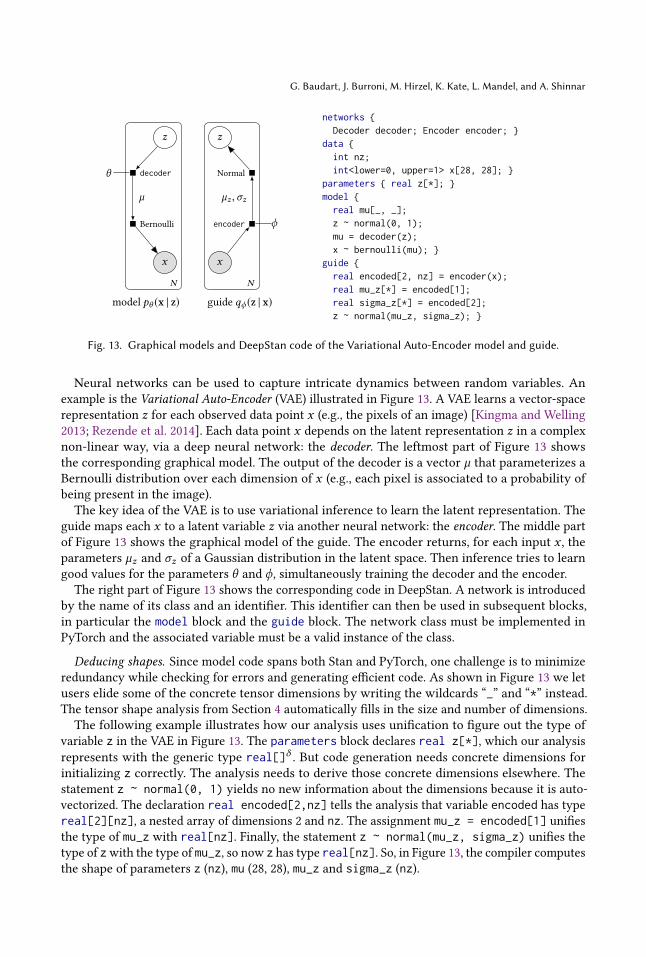
networks {Decoder decoder; Encoder encoder; }

data {int nz;int<lower=0, upper=1> x[28, 28]; }

parameters { real z[*]; }model {

real mu[_, _];z ~ normal(0, 1);mu = decoder(z);x ~ bernoulli(mu); }

guide {real encoded[2, nz] = encoder(x);real mu_z[*] = encoded[1];real sigma_z[*] = encoded[2];z ~ normal(mu_z, sigma_z); }

Fig. 13. Graphical models and DeepStan code of the Variational Auto-Encoder model and guide.

Neural networks can be used to capture intricate dynamics between random variables. An

example is the Variational Auto-Encoder (VAE) illustrated in Figure 13. A VAE learns a vector-space

representation z for each observed data point x (e.g., the pixels of an image) [Kingma and Welling

2013; Rezende et al. 2014]. Each data point x depends on the latent representation z in a complex

non-linear way, via a deep neural network: the decoder. The leftmost part of Figure 13 shows

the corresponding graphical model. The output of the decoder is a vector µ that parameterizes a

Bernoulli distribution over each dimension of x (e.g., each pixel is associated to a probability of

being present in the image).

The key idea of the VAE is to use variational inference to learn the latent representation. The

guide maps each x to a latent variable z via another neural network: the encoder. The middle part

of Figure 13 shows the graphical model of the guide. The encoder returns, for each input x , theparameters µz and σz of a Gaussian distribution in the latent space. Then inference tries to learn

good values for the parameters θ and ϕ, simultaneously training the decoder and the encoder.

The right part of Figure 13 shows the corresponding code in DeepStan. A network is introduced

by the name of its class and an identifier. This identifier can then be used in subsequent blocks,

in particular the model block and the guide block. The network class must be implemented in

PyTorch and the associated variable must be a valid instance of the class.

Deducing shapes. Since model code spans both Stan and PyTorch, one challenge is to minimize

redundancy while checking for errors and generating efficient code. As shown in Figure 13 we let

users elide some of the concrete tensor dimensions by writing the wildcards “_” and “*” instead.The tensor shape analysis from Section 4 automatically fills in the size and number of dimensions.

The following example illustrates how our analysis uses unification to figure out the type of

variable z in the VAE in Figure 13. The parameters block declares real z[*], which our analysis

represents with the generic type real[]δ . But code generation needs concrete dimensions for

initializing z correctly. The analysis needs to derive those concrete dimensions elsewhere. The

statement z ~ normal(0, 1) yields no new information about the dimensions because it is auto-

vectorized. The declaration real encoded[2,nz] tells the analysis that variable encoded has type

real[2][nz], a nested array of dimensions 2 and nz. The assignment mu_z = encoded[1] unifies

the type of mu_z with real[nz]. Finally, the statement z ~ normal(mu_z, sigma_z) unifies thetype of zwith the type of mu_z, so now z has type real[nz]. So, in Figure 13, the compiler computes

the shape of parameters z (nz), mu (28, 28), mu_z and sigma_z (nz).


x

mlpθ

λ

Cat.

l

N

p(θ | x, l)

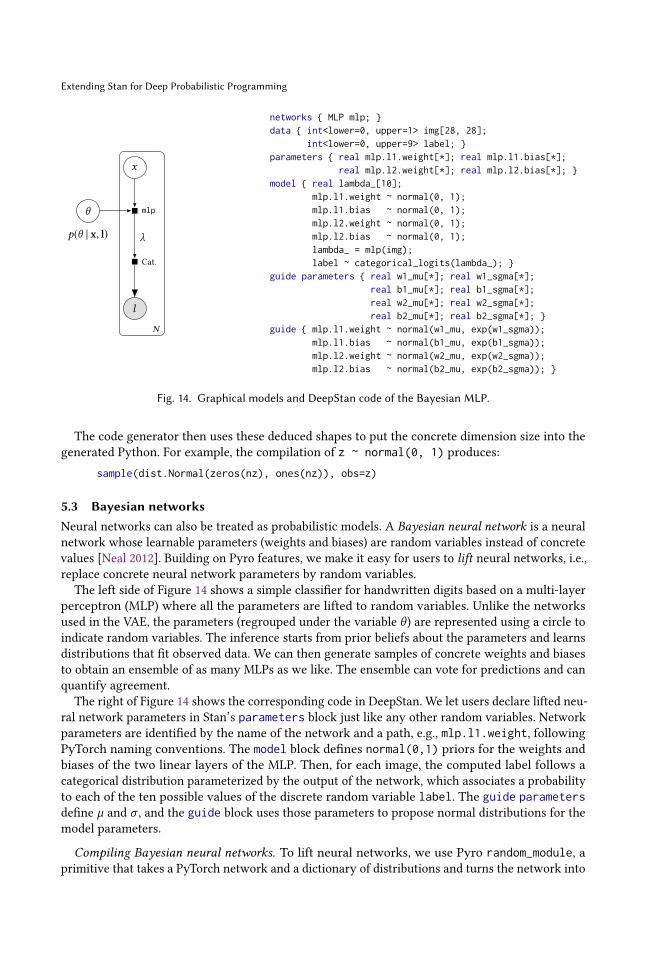
networks { MLP mlp; }data { int<lower=0, upper=1> img[28, 28];

int<lower=0, upper=9> label; }parameters { real mlp.l1.weight[*]; real mlp.l1.bias[*];

real mlp.l2.weight[*]; real mlp.l2.bias[*]; }model { real lambda_[10];

mlp.l1.weight ~ normal(0, 1);mlp.l1.bias ~ normal(0, 1);mlp.l2.weight ~ normal(0, 1);mlp.l2.bias ~ normal(0, 1);lambda_ = mlp(img);label ~ categorical_logits(lambda_); }

guide parameters { real w1_mu[*]; real w1_sgma[*];real b1_mu[*]; real b1_sgma[*];real w2_mu[*]; real w2_sgma[*];real b2_mu[*]; real b2_sgma[*]; }

guide { mlp.l1.weight ~ normal(w1_mu, exp(w1_sgma));mlp.l1.bias ~ normal(b1_mu, exp(b1_sgma));mlp.l2.weight ~ normal(w2_mu, exp(w2_sgma));mlp.l2.bias ~ normal(b2_mu, exp(b2_sgma)); }

Fig. 14. Graphical models and DeepStan code of the Bayesian MLP.

The code generator then uses these deduced shapes to put the concrete dimension size into the

generated Python. For example, the compilation of z ~ normal(0, 1) produces:

sample(dist.Normal(zeros(nz), ones(nz)), obs=z)

5.3 Bayesian networksNeural networks can also be treated as probabilistic models. A Bayesian neural network is a neural

network whose learnable parameters (weights and biases) are random variables instead of concrete

values [Neal 2012]. Building on Pyro features, we make it easy for users to lift neural networks, i.e.,replace concrete neural network parameters by random variables.

The left side of Figure 14 shows a simple classifier for handwritten digits based on a multi-layer

perceptron (MLP) where all the parameters are lifted to random variables. Unlike the networks

used in the VAE, the parameters (regrouped under the variable θ ) are represented using a circle to

indicate random variables. The inference starts from prior beliefs about the parameters and learns

distributions that fit observed data. We can then generate samples of concrete weights and biases

to obtain an ensemble of as many MLPs as we like. The ensemble can vote for predictions and can

quantify agreement.

The right of Figure 14 shows the corresponding code in DeepStan. We let users declare lifted neu-

ral network parameters in Stan’s parameters block just like any other random variables. Network

parameters are identified by the name of the network and a path, e.g., mlp.l1.weight, followingPyTorch naming conventions. The model block defines normal(0,1) priors for the weights andbiases of the two linear layers of the MLP. Then, for each image, the computed label follows a

categorical distribution parameterized by the output of the network, which associates a probability

to each of the ten possible values of the discrete random variable label. The guide parametersdefine µ and σ , and the guide block uses those parameters to propose normal distributions for the

model parameters.

Compiling Bayesian neural networks. To lift neural networks, we use Pyro random_module, aprimitive that takes a PyTorch network and a dictionary of distributions and turns the network into


(a) Double normal

parameters {

real theta;

}

model {

theta ~ normal(1000, 1);

theta ~ normal(1000, 1);

}

(b) Linear Regression

data {

int<lower=0> N;

vector[N] x;

vector[N] y;

}

parameters {

real alpha;

real beta;

real<lower=0> sigma;

}

model {

y ~ normal(alpha + beta * x,

sigma);

}

(c) Reparameterization

parameters {

real y_std;

real x_std;

}

transformed parameters {

real y = 3.0 * y_std;

real x = exp(y/2) * x_std;

}

model{

y_std ~ normal(0, 1);

x_std ~ normal(0, 1);

}

Fig. 15. Basic examples for the comparison of Stan and DeepStan

a distribution of networks where each parameter is sampled from the corresponding distribution.

We treat network parameters as any other random variables, that is, we apply the comprehensive

translation from Section 2.3. This translation initializes parameters with a uniform prior.

priors = {}

priors['l1.weight'] = ImproperUniform(shape=mlp.l1.weight.shape)

... # priors of the other parameters

lifted_mlp = pyro.random_module('mlp', mlp, priors)()

Then, the Stan ~ statements in the model block are compiled into Pyro observe statements.

mlp_params = dict(lifted_mlp.named_parameters())

sample('l1.weight', Normal(zeros(mlp.l1.weight.size()), ones(mlp.l1.weight.size())),

obs=mlp_params['l1.weight'])

It is also possible to mix probabilistic parameters and non-probabilistic parameters. Our transla-

tion only lifts the parameters that are declared in the parameters block by only adding those to

the priors dictionary.

6 EVALUATIONThis section evaluates DeepStan on multiple examples. To test our compilation scheme, for a subset

of examples, we run inference on the generated Pyro code using NUTS (No U-Turn Sampler [Homan

andGelman 2014], an optimizedHMCwhich is the preferred inferencemethod for Stan, and compare

the results with Stan (Section 6.1). We show on a simple example that, sometimes, using explicit

VI gives comparable or even more accurate results (Section 6.1). Finally, for deep probabilistic

models, we compare the generated Pyro code against hand-written code and find comparable

results (Section 6.2).

6.1 Comparison of Stan and DeepStanThis section describes eight experiments comparing inference output from Stan and DeepStan. The

first four examples exercise our translation techniques on simple models with no data or synthetic

data. Coin is the example presented Figure 1. Double normal is doing multiple updates of the same


Table 2. Comparison of execution time and parameter distributions between Stan and DeepStan.

Stan DeepStan/Pyro DeepStan/NumPyro

time(s) time(s) KS p-value time(s) KS p-value

coin 110 + 0.3 219 0.41 (z) 70 0.41 (z)double normal 107 + 0.2 76 0.34 (theta) 57 0.66 (theta)reparameterization 121 + 0.7 114 0.50 (x_std) 117 0.40 (y)linear regression 85 + 0.5 348 0.23 (beta) 61 0.26 (sigma)

aspirin 70 + 0.8 635 0.32 (tau) 83 0.16 (theta_raw[4])roaches 73 + 6.8 551 0.30 (beta[2]) 38 0.50 (beta[3])8 schools 67 + 1.0 842 0.38 (theta[5]) 58 0.12 (eta[6])seeds 66 + 3.4 1,081 0.29 (sigma) 74 0.21 (b[3])

parameter theta (Figure 15a). Linear Regression is the simplest linear regression model (Figure 15b).

Reparameterization is the reparameterized Neal’s funnel example that uses transformed parameters

(Figure 15c). The last four examples, aspirin, roaches,1 8 schools, and seeds, are popular hierarchicalmodels with real data that are taken from the Stan examples git repository.

2These examples are

also used for comparing SlicStan to Stan in [Gorinova et al. 2019].

Experimental setup. Pyro offers two implementation of NUTS, one leveraging PyTorch (classic

Pyro), and another one based on Numpy and JAX (NumPyro). We ran the experiments with these

two runtimes and compared the computed distributions with the results of Stan.

Experiments were run in parallel on a Linux server with 32 cores (2GHz, 242 GB RAM) with the

latest version of Pyro (1.3.1), NumPyro (0.2.4), and PyStan (2.19.1.1). The inference method is NUTS

with 10,000 sampling steps, 1,000 warmup steps, and 1 Markov chain. To reduce the autocorrelation

of the samples and increase the effective sample size, we then used a thinning factor of 10 (i.e.,

select one sample every 10 draws).

For each parameter, we compare the posterior marginal distributions generated by Stan and

DeepStan using a two-sample Kolmogorov-Smirnov (KS) test on all the parameters. For multidi-

mensional parameters we run the KS test for every component. If the p-value of the KS test is above

the significance level (e.g., >0.05), we cannot reject the hypothesis that the distributions of the two

samples are the same.

Results. Table 2 summarizes the results of our experiments. For each model, we report the

compilation and execution time for Stan, the execution time of the two Pyro runtimes, and the

parameter with the lowest p-value for the KS test. All the results are averaged over 10 runs (times

and KS test results). Since none of the the KS p-values are below the significance level, these results

empirically validate that our translation from DeepStan to Pyro preserves the Stan semantics.

Stan first compiles the model to C++ and compiles the C++ code, which takes significant time,

but the inference is impressively fast. In comparison, the compilation from DeepStan to Pyro is

quasi-instantaneous, but the Pyro version of NUTS is significantly slower. NumPyro was intro-

duced to mitigate this issue by leveraging Numpy efficient vectorization and JAX just-in-time

compilation (JIT). Table 2 shows that, while NumPyro is in average significantly faster than classic

Pyro on our set of examples (with the notable exception of Reparameterization), it is still much

slower than Stan.

1We adapted the roaches model with priors found in https://avehtari.github.io/modelselection/roaches.html

2https://github.com/stan-dev/example-models

https://avehtari.github.io/modelselection/roaches.html

https://github.com/stan-dev/example-models


0

1000DeepStanSVIStan

0 10 200

1000DeepStanSVIDeepStan

parameters {real cluster;real theta; }

model {real mu;cluster ~ normal(0, 1);if (cluster > 0) mu = 20;else mu = 0;theta ~ normal(mu, 1); }

guide parameters {real mc;real m1; real m2;real ls1; real ls2; }

guide {cluster ~ normal(mc, 1);if (cluster > 0) theta ~ normal(m1, exp(ls1));else theta ~ normal(m2, exp(ls2)); }

Fig. 16. DeepStan code and histograms of the multimodal example using Stan, DeepStan with NUTS, andDeepStan with VI.

Explicit variational guide. The multimodal example shown in Figure 16 is a mixture of two

Gaussian distributions with different means but identical variances. The histograms in the left

half of Figure 16 show that in both Stan and DeepStan, this example is particularly challenging

for NUTS. Using multiple chains, NUTS finds the two modes, but the chains do not mix and the

relative densities are incorrect.

This is a known limitation of HMC.3As shown in the code of Figure 16 we can provide a custom

variational guide that will correctly infer the two modes (DeepStanSVI). Note, however, that this

approach requires a priori knowledge about the shape of the true posterior.

6.2 Deep probabilistic modelsSince Stan lacks support for deep probabilistic models, we could not use it as a baseline. Instead,

we compare the performance of the code generated by our compiler with hand-written Pyro code

on the VAE described in Section 5.2 and a simple Bayesian neural network.

VAE. Variational autoencoders were not designed as a predictive model but as a generative

model to reconstruct images. Evaluating the performance of a VAE is thus non-obvious. We use

the following experimental setting. We trained two VAEs on the MNIST dataset using VI: one

hand-written in Pyro, the other written in DeepStan. For each image in the test set, the trained

VAEs compute a latent representation of dimension 5. We then cluster these representations using

KMeans with 10 clusters. Then we measure the performance of a VAE with the pairwise F1 metric:

true positives are the number of images of the same digit that appear in the same cluster. For Pyro

F1=0.41 (precision=0.43, recall=0.40), and for DeepStan F1=0.43 (precision=0.44, recall=0.42). These

numbers shows that compiling DeepStan to Pyro does not impact the performance of such deep

probabilistic models.

Bayesian MLP. We trained two versions of a 2-levels Bayesian multi-layer perceptron (MLP)

where all the parameters are lifted to random variables (see section 5.3): one hand-written in Pyro,

the other written in DeepStan. We trained both models for 20 epochs on the training set. For each

model we then generated 100 samples of concrete weights and biases to obtain an ensemble MLP.

3https://mc-stan.org/users/documentation/case-studies/identifying_mixture_models.html

https://mc-stan.org/users/documentation/case-studies/identifying_mixture_models.html


The log-likelihood of the test set is then computed for each MLP. We observe that the log-likelihood

distribution is indistinguishable for the two models (KS p-value: 0.99) and the execution time is

about the same. Again, these experiments show that compiling DeepStan models to Pyro has little

impact on the model. Additionally, we observe that changing the priors on the network parameters

from normal(0,1) to normal(0,10) (see section 5.3) increases the accuracy of the models from 0.92

to 0.96. This further validates our compilation scheme where priors on parameters are compiled to

observe statements on deep probabilistic models.

7 RELATEDWORKTo the best of our knowledge, we propose the first comprehensive translation of Stan to a generative

PPL. The closest related work has been developed by the Pyro team [Chen et al. 2018]. Their work

focuses on performance and our work on completeness. Their proposed compilation technique

corresponds to the generative translation presented in Section 2.1 and thus only handles a subset

of Stan. Compared to our approach, they are also looking into independence assumptions between

loop iterations to generate parallel code. Combining these ideas with our approach, in particular

leveraging our type system to add independence assumptions, is a promising future direction.

They do not extend Stan with VI and neural networks. Appendix B.2 of [Gorinova et al. 2018] also

outlines the generative translation of Section 2.1, but also mention the issue with multiple updates.

The goal of compiling Stan to Pyro is not to replace Stan’s highly optimized inference en-

gine [Homan and Gelman 2014], but rather to create a platform for experimenting with new ideas.

As an example, Section 5.1 showed how to extend Stan with explicit variational guides. In the same

vein, Pyro now offers tools for automatic variational guide synthesis [Blei et al. 2017] that can now

be tested on existing Stan models.

In recent years, taking advantage of the maturity of DL frameworks, multiple deep probabilistic

programming languages have been proposed: Edward [Tran et al. 2017] and ZhuSuan [Shi et al.

2017] built on top of TensorFlow, Pyro [Bingham et al. 2019] and ProbTorch [Siddharth et al.

2017] built on top of PyTorch, and PyMC3 [Salvatier et al. 2015] built on top of Theano. All these

languages are implemented as libraries. The users thus need to master the entire technology stack

of the library, the underlying DL framework, and the host language. In comparison, DeepStan is a

self-contained language and the compiler helps the programmer via dedicated static analyses (e.g.,

the tensor dimension analysis of Section 5.2).

Finally, Section 4 presents a type system for tensor shape analysis. Previous work on efficiently

executing matlab performs a similar analysis using an algebraic approach [Joisha et al. 2003].

8 CONCLUSIONThis paper proves a comprehensive compilation scheme from Stan to any generative probabilistic

programming language. We thus show that Stan is at most as expressive as this family of languages.

To validate our approach we implemented a compiler from Stan to Pyro. Additionally, we designed

and implemented extensions for Stan with explicit variational guides and neural networks.

REFERENCESEli Bingham, Jonathan P. Chen, Martin Jankowiak, Fritz Obermeyer, Neeraj Pradhan, Theofanis Karaletsos, Rohit Singh,

Paul Szerlip, Paul Horsfall, and Noah D. Goodman. 2019. Pyro: Deep Universal Probabilistic Programming. Journal ofMachine Learning Research (JMLR) 20 (2019), 1–6. http://www.jmlr.org/papers/volume20/18-403/18-403.pdf

David M. Blei, Alp Kucukelbir, and Jon D. McAuliffe. 2017. Variational Inference: A Review for Statisticians. J. Amer. Statist.Assoc. 112 (2017), 859–877. Issue 518.

Bradley P Carlin and Thomas A Louis. 2008. Bayesian methods for data analysis. CRC Press.

Bob Carpenter, Andrew Gelman, Matthew D Hoffman, Daniel Lee, Ben Goodrich, Michael Betancourt, Marcus Brubaker,

Jiqiang Guo, Peter Li, and Allen Riddell. 2017. Stan: A probabilistic programming language. Journal of Statistical Software

http://www.jmlr.org/papers/volume20/18-403/18-403.pdf


76, 1 (2017), 1–37.

Jonathan P. Chen, Rohit Singh, Eli Bingham, and Noah Goodman. 2018. Transpiling Stan models to Pyro. In The InternationalConference on Probabilistic Programming.

Marco F. Cusumano-Towner, Feras A. Saad, Alexander K. Lew, and Vikash K. Mansinghka. 2019. Gen: A General-Purpose

Probabilistic Programming System with Programmable Inference. In Conference on Programming Language Design andImplementation (PLDI). 221–236. https://doi.org/10.1145/3314221.3314642

Luc De Raedt and Kristian Kersting. 2008. Probabilistic inductive logic programming. In Probabilistic Inductive LogicProgramming. Springer, 1–27.

Luc De Raedt, Angelika Kimmig, and Hannu Toivonen. 2007. ProbLog: A Probabilistic Prolog and Its Application in Link

Discovery.. In IJCAI, Vol. 7. Hyderabad, 2462–2467.Andrew Gelman and Jennifer Hill. 2006. Data analysis using regression and multilevel/hierarchical models. Cambridge

university press.

Andrew Gelman, Hal S Stern, John B Carlin, David B Dunson, Aki Vehtari, and Donald B Rubin. 2013. Bayesian data analysis.Chapman and Hall/CRC.

Noah Goodman, Mansinghka Vikash, Daniel Roy, Keith Bonawitz, and Joshua Tenenbaum. 2008. Church: a Language for

Generative Models. In Conference on Uncertainty in Artificial Intelligence (UAI). 220–229.Noah D. Goodman and Andreas Stuhlmüller. 2014. The Design and Implementation of Probabilistic Programming Languages.

http://dippl.org Accessed February 2019.

Andrew D. Gordon, Thomas A. Henzinger, Aditya V. Nori, and Sriram K. Rajamani. 2014. Probabilistic Programming. In

ICSE track on Future of Software Engineering (FOSE). 167–181.Maria I. Gorinova, Andrew D. Gordon, and Charles Sutton. 2018. SlicStan: Improving Probabilistic Programming using

Information Flow Analysis. In Workshop on Probabilistic Programming Languages, Semantics, and Systems (PPS). https://pps2018.soic.indiana.edu/files/2017/12/SlicStanPPS.pdf

Maria I. Gorinova, Andrew D. Gordon, and Charles A. Sutton. 2019. Probabilistic programming with densities in SlicStan:

efficient, flexible, and deterministic. PACMPL 3, POPL (2019), 35:1–35:30.

Matthew D. Homan and Andrew Gelman. 2014. The No-U-turn Sampler: Adaptively Setting Path Lengths in Hamiltonian

Monte Carlo. J. Mach. Learn. Res. 15, 1 (Jan. 2014), 1593–1623. http://dl.acm.org/citation.cfm?id=2627435.2638586

Pramod G. Joisha, U. Nagaraj Shenoy, and Prithviraj Banerjee. 2003. Computing Array Shapes in MATLAB. In Languagesand Compilers for Parallel Computing, Henry G. Dietz (Ed.). Springer Berlin Heidelberg, Berlin, Heidelberg, 395–410.

Diederik P. Kingma and Max Welling. 2013. Auto-Encoding Variational Bayes. https://arxiv.org/abs/1312.6114Dexter Kozen. 1981. Semantics of Probabilistic Programs. J. Comput. System Sci. 22, 3 (1981), 328–350.David Lunn, Chris Jackson, Nicky Best, Andrew Thomas, and David Spiegelhalter. 2012. The BUGS Book: A Practical

Introduction to Bayesian Analysis. Chapman and Hall/CRC.

David Lunn, David Spiegelhalter, Andrew Thomas, and Nicky Best. 2009. The BUGS project: Evolution, critique and future

directions. Statistics in medicine 28, 25 (2009), 3049–3067.Vikash Mansinghka, Daniel Selsam, and Yura Perov. 2014. Venture: a higher-order probabilistic programming platform with

programmable inference. arXiv preprint arXiv:1404.0099 (2014).Andrew McCallum, Karl Schultz, and Sameer Singh. 2009. Factorie: Probabilistic programming via imperatively defined

factor graphs. In Advances in Neural Information Processing Systems. 1249–1257.Brian Milch, Bhaskara Marthi, Stuart J. Russell, David Sontag, Daniel L. Ong, and Andrey Kolobov. 2005. BLOG: Probabilistic

Models with Unknown Objects. In International Joint Conference on Artificial Intelligence (IJCAI). 1352–1359.Lawrence M. Murray and Thomas B. Schön. 2018. Automated learning with a probabilistic programming language: Birch.

Annual Reviews in Control 46 (2018), 29 – 43.

Radford M. Neal. 2012. Bayesian Learning for Neural Networks. Vol. 118. Springer.Adam Paszke, Sam Gross, Soumith Chintala, Gregory Chanan, Edward Yang, Zachary DeVito, Zeming Lin, Alban Desmaison,

Luca Antiga, and Adam Lerer. 2017. Automatic Differentiation in PyTorch. In AutoDiff Workshop.Avi Pfeffer. 2001. IBAL: A Probabilistic Rational Programming Language. In International Joint Conference on Artificial

Intelligence (IJCAI). 733–740.Avi Pfeffer. 2009. Figaro: An object-oriented probabilistic programming language. Charles River Analytics Technical Report

137 (2009), 96.

Martyn Plummer et al. 2003. JAGS: A program for analysis of Bayesian graphical models using Gibbs sampling. In Proceedingsof the 3rd international workshop on distributed statistical computing, Vol. 124. Vienna, Austria.

Danilo J. Rezende, Shakir Mohamed, and Daan Wierstra. 2014. Stochastic Backpropagation and Approximate Inference in

Deep Generative Models. In International Conference on Machine Learning (ICML). 1278–1286.John Salvatier, Thomas V. Wiecki, and Christopher Fonnesbeck. 2015. Probabilistic Programming in Python Using PyMC3.

https://arxiv.org/abs/1507.08050

https://doi.org/10.1145/3314221.3314642

http://dippl.org

https://pps2018.soic.indiana.edu/files/2017/12/SlicStanPPS.pdf

https://pps2018.soic.indiana.edu/files/2017/12/SlicStanPPS.pdf

http://dl.acm.org/citation.cfm?id=2627435.2638586

http://dl.acm.org/citation.cfm?id=2627435.2638586




Jiaxin Shi, Jianfei. Chen, Jun Zhu, Shengyang Sun, Yucen Luo, Yihong Gu, and Yuhao Zhou. 2017. ZhuSuan: A Library for

Bayesian Deep Learning. https://arxiv.org/abs/1709.05870N. Siddharth, Brooks Paige, Jan-Willem van de Meent, Alban Desmaison, Noah D. Goodman, Pushmeet Kohli, Frank

Wood, and Philip Torr. 2017. Learning Disentangled Representations with Semi-Supervised Deep Generative Models. In

Conference on Neural Information Processing Systems (NIPS). 5927–5937.Sam Staton. 2017. Commutative Semantics for Probabilistic Programming. In European Symposium on Programming (ESOP).

855–879.

Sam Staton, Hongseok Yang, Frank D. Wood, Chris Heunen, and Ohad Kammar. 2016. Semantics for probabilistic program-

ming: higher-order functions, continuous distributions, and soft constraints. In Symposium on Logic in Computer Science(LICS). 525–534.

David Tolpin, Jan-Willem van de Meent, Hongseok Yang, and Frank Wood. 2016. Design and Implementation of Probabilistic

Programming Language Anglican. In Symposium on the Implementation and Application of Functional ProgrammingLanguages (IFL). 6:1–6:12.

Dustin Tran, Matthew D. Hoffman, Rif A. Saurous, Eugene Brevdo, Kevin Murphy, and David M. Blei. 2017. Deep Probabilistic

Programming. In International Conference on Learning Representations (ICLR).Jan-Willem van de Meent, Brooks Paige, Hongseok Yang, and Frank Wood. 2018. An introduction to probabilistic program-

ming. arXiv preprint arXiv:1809.10756 (2018).


extending stan for deep probabilistic programming › pdf › 1810.00873.pdf · stan that can learn...

Documents