extending verilog-a for compact modeling -...

April 2, 2004

1 of 22

Version 7 Describes the changes that should be made to the Verilog-A and Verilog-AMS language definition [1] to

better support compact device modeling [2]. This document is a product of an Accellera subcommittee

which started work in May 2003 and included participants from the compact modeling community,

semiconductor companies, and EDA vendor companies.

Proposed Verilog-A

Language Extensions for

Compact Modeling

Proposed Verilog-A Language Extensions for Compact Modeling Parameters and Variables

2 of 22

1.0 Parameters and Variables

1.1 Descriptions and units

Parameter declarations should provide a method for specifying the units of the parameter and a text

description. This information would be used to generate documentation and help messages. For exam-

ple, “spectre -help bsim4” or “hpeesof_sim -help BSIM4” instructs the respective simulator to print a

description of Berkeley’s BSIM4 compact model, including a list of parameters with units and descrip-

tions.

Examples:

parameter real freq=1G “Hz” from (0:inf) (*desc=“Center frequency”*);parameter real kvco=1G “Hz/V” from (0:inf) (*desc=“Gain of VCO”*);parameter integer resolution=8 “bits” from [1:30] (*desc=“Quantization level of converter”*);

Variables declared at module scope (outside the analog block) should also be allowed to have units and

descriptions. Those that do should be considered “output or operating point parameters,” meaning that

simulators should print the name, value, units, and description of these variables (and no others) when

printing operating-poing information for the circuit. Operating point values, such as vth, vdsat, or cgsfor the BSIM4 compact model, are frequently used in the design of circuits. (See also §3.2 for operating

point values that are computed using derivatives.)

Examples:

real vdsat “V” (*desc=“drain-source saturation voltage”*);real cgs “F” (*desc=“gate-source capacitance”*);

Since essentially all compact model parameters should be described in such a way, it is important to

have an efficient and standard method of attaching this information. However, since the text description

does not affect the numerical results of the simulation, it is reasonable to place this as an attribute; digi-

tal Verilog simulators will be able to ignore this attribute.

Note that there is no precedent for a standardized attribute in Verilog-AMS nor Verilog 2001. The Sys-

temVerilog committee is apparently considering some standard attributes. We would like to standardize

this attribute so that all SPICE -like simulators will work the same.

Units may affect the simulation, in particular through the ‘timescale directive in Verilog 1364-1995,

and hence parameter units should not be implemented through an attribute. The ‘timescale directive is

unfortunate, since it affects numbers throughout the module. We do not propose that any “units mathe-

matics” be performed; however, it should be clear to the user what the units are. BSIM3 allowed one to

specify the parameter U0 in non-MKS units; if the value was greater than 1.0, it was assumed to have

been specified in cm2/Vs instead of m2/Vs.

Proposal: for parameters, change Syntax 3-2 and the corresponding lines of A.4 as follows.

declarator_init ::=

parameter_identifier = constant_expression range_description

| parameter_array_identifier range = constant_param_arrayinit range_description

range_description ::=

[units_string] { opt_value_range } [ (*desc=description_string*)]


3 of 22

Proposal: for variables, create new declaration syntax for output_integer_declaration and

output_real_declaration.

output_integer_declaration ::=

integer list_of_output_identifiers ;

output_real_declaration ::=

real list_of_output_identifiers ;

list_of_output_identifiers ::=

output_var_name { , output_var_name }

output_var_name ::=

variable_identifier

| array_identifier array_range

[units_string] [(*desc= description_string *)]

array_range ::=

[ upper_limit_constant_expression : lower_limit_constant_expression ]

These new output declarations will be syntactically restricted to occur only at module scope; see §1.6.

They replace integer_declaration and real_declaration at that scope, since the attribute is optional;

integer_declaration and real_declaration will remain defined for block_item_declarations.

1.2 Detecting whether a parameter was specified

There are currently many instances in existing compact models where the code checks whether the user

actually specified a value for a parameter. This detection is often used for overrides, where an unspeci-

fied parameter is determined from others; Verilog-A already supports computation of default values

from (previously-declared) parameters. However, in some cases, the override equation is very compli-

cated, and sometimes it is circular. One example of circularity involves kp and uo in MOS level-3 mod-

els; these parameters take their defaults from each other. If uo is specified, kp takes its default from

kp=uo*tox. If uo is not specified, but kp is, then uo is calculated from kp. This circularity cannot be

achieved presently in Verilog-A within the parameter declaration syntax. The BSIM3 threshold voltage

is another example: one may specify it through the flatband voltage vfb or through vth0; the calculation

of one from the other is much more complicated than in the MOS level-3 model. In the Verilog-A mod-

els that Silvaco has posted on the web [3], vfb, vth0, and vtho (an alias for vth0) all have default values

of -99.0, which acts as a flag for making the correct computation. This method is not elegant nor gener-

ally applicable, since -99.0 (or any other value) might be a legitimate value for a particular parameter.

Even when there are illegal values of the parameters that could be used as flags, this will likely force the

parameter range to include other illegal values. Using a negative value for BSIM3’s cgdo parameter

means that the range for cgdo cannot forbid negative values. Further, any simulator that reports model

card values for the simulation as part of an operating-point report will print these strange values.

A much better solution would be to provide a method of directly checking whether a parameter was

specified. A reasonable default value may then be provided. ADMS [4] has a $given function and


4 of 22

Cadence reportedly provides the $param_given function (in internal versions of their simulator) for the

purpose of determining whether a parameter value as been specified.

Proposal: add the $param_given system task, which can appear in a genvar_expression as well as an

expression. The returned value would be one (1) if the parameter was specified either by its name or one

of its aliases, or zero (0) if its value was computed from the default expression.

genvar_primary ::=

constant_primary

| genvar_identifier

| genvar_identifier [ genvar_expression ]

| analog_system_task

analog_system_task ::=

analysis( arg_list)| $param_given(module_parameter_identifier)| $port_connected(port_scalar_expression)

See §4.1 for $port_connected.

The argument to $param_given must be a parameter name, not an alias (see the next section).

One might want to ask about more than parameter in a single call, but it is not clear whether the result

should be true if all parameters are given or true if any of the parameters is given. The former would

likely be more useful (if all the required parameters are specified, then use them to make a calculation).

However, this would be inconsistent with the analysis() function, which returns true if any of its argu-

ments matches the current analysis type.

1.3 Parameter aliases

To support backward compatibility to older models, and to provide convenient alternatives for parame-

ter values, parameter aliases should be supported. For example, in older BJT models the vaf and varparameters are named va and vb. The values specified for aliased parameters are treated as though the

user had specified using the target name. Thus, if the user specified va=20, the simulator treats it as if

the user had specified vaf=20, and if the simulator reports the values of parameters for the simulation, it

would list the value under vaf and not under va. Also, when the user asks for help, the vaf parameter is

listed, but the va parameter is not.

Although some of this functionality can be handled by the language as it exists today by chaining

defaults, there are two drawbacks. Consider vaf and va as an example. If the parameters are declared

with

parameter real va = inf;parameter real vaf = va;

and the model equations use vaf, then the user may specify either and get the right behavior. However, it

is not possible to prevent both from being specified (with different values), and both parameters would

appear in a list of parameter values generated by the simulator. Consider also the parameter used to indi-

cate a difference in device temperature relative to the circuit, called variously trise (Cadence’s Spectre),

dtemp (Synopsys’ HSpice), or dta (Philips’ Mextram 504 model). Even if the aliased parameters all had

the same value, there is potential confusion; if all three were specified as 10, or if the simulator printed a

value of 10 for each alias, the user might think or expect that the device was 30 degrees above ambient.


5 of 22

Proposal: add the keyword aliasparam and use the syntax

parameter_alias_declaration ::=

aliasparam alias_identifier = parameter_identifier;

Model equations must be written in terms of the original parameter name (vaf). Multiple aliases may be

assigned to a single parameter. An alias_identifier may not conflict with a parameter_identifier. The

simulator should report an error if a parameter is specified by more than one name (an alias and the

original parameter name or two aliases), either on the instance line or though a paramset (see §2.0).

Note that aliasparam handles only exact aliases. SPICE allows one to specify the device temperature

directly with the parameter temp, rather than as an offset from $temperature as is done for trise. One

would need to use $param_given to allow a model to use either.

1.4 Multiplicity factor

This is an extremely important capability. It is heavily used and valued by designers. The multiplicity

factor is a parameter m that can be applied to an instance of a model that acts to scale the instance in

such a way that there appear to be m instances in parallel. This parameter must be handled hierarchi-

cally, so that if one instance is contained in another, then the effective multiplicity factor of the first

instance is the product of multiplicity factors explicitly specified for both.

The omission of the multiplicity factor from the Verilog-AMS LRM led to some unfortunate inconsis-

tencies. Within a Verilog-A netlist or module, one may reference a subcircuit defined in SPICE or in

native Verilog-AMS, but only the SPICE subcircuit will accept the multiplicity factor.

The actual behavior of the multiplicity factor must be handled automatically by the simulator rather than

forcing the user to explicitly code the proper behavior in to the model. The latter would result in multi-

plicity factors being inconsistently or incorrectly implemented and interpreted, which would eventually

make the multiplicity factor useless. As such, the multiplicity factor must be an implicit parameter to

each instance that multiplies the (deterministic) current contributed to any node or branch by the

instance and divides the (deterministic) current probed by the instance. Note that, while deterministic

current contributions should be scaled by m, noise currents should be scaled by m1/2 and noise voltage

by m–1/2.

In principle, mismatch parameters should also be scaled by m–1/2. For example, if there are m resistors in

parallel, each with a given standard deviation σ of their resistance, the parallel combination will have a

standard deviation of resistance equal to σ/m1/2. However, there is presently no method in Verilog-A for

requesting a random variable with a particular standard deviation. Hence, the module can only treat the

standard deviation as an offset, and any Monte-Carlo or Monte-Carlo-like simulations must be handled

at a different level.

An unfortunate consequence of this decision to handle m automatically is that the simulator will likely

have to implement this as a post-processing of all branch quantities and their derivatives for each itera-

tion of each timepoint. Some compact models use the multiplicty factor to pre-scale parameters once for

an analysis. We recognize this inefficiency, but feel that it is justified in the quest for ensuring correct

implementation of the multiplicity factor for all models. We note that, for compact models of moderate

complexity, the multiplications will probably not be a significant fraction of the floating-point opera-

tions involved in calculating the model. Further, the simulator may be able to find a way to optimize the

scaling.

In addition to the automatic scaling of currents, there are times when the multiplicity factor would rea-

sonably expected to affect the values of output and operating point parameters (§1.4). For example, con-

sider a resistor whose effective resistance is computed by r = (w*rsh)/(l*m); one might also want to


6 of 22

compute the effective current or power of the resistor. Not providing access to the multiplicity factor

provides a certain consistency; all output and operating point parameters would necessarily be com-

puted from the perspective of the individual elements of the parallel array. However, that is not always

what the users want, so there is value in providing composite quantities. However, the model writer

must not be allowed to interfere with the proper interpretation of the multiplicity factor, so that if the

value of the multiplicity factor is made available in the module, it must not be allowed to affect the

behavior of the model (the behavior of the model has already been appropriately modified by the simu-

lator). For this reason, it should be an error for the output signal values to depend on the value of the

multiplicity factor that is explicitly made available within the module.

The effect of OOMRs, or “out of module references,” must be considered. OOMRs are the observation

of one module’s signals or variables from another module. The variables in a module will not be scaled

by m, because the simulator will not know what the proper scaling is (unless it is an output parameter

that the model writer has scaled), so necessarily variables referenced out-of-module must refer to a

value for a one of the m parallel devices. On the other hand, it seems that signals, specifically currents,

referenced out-of-module should refer to the actual current in the branch, for all the devices in compos-

ite. If the module that asks for the OOMR is a current-dependent source, it should get the correct cur-

rent. This inconsistency may be confusing for model writers.

One last issue to consider is rmin. Some simulators (e.g., Cadence’s Spectre) eliminate a parasitic resis-

tor if its value falls below a certain threshold, called rmin. If we do not allow access to m from within

the model, we cannot determine the actual value of a resistor, only the unscaled value. This could be

addressed with a branch parameter (a concept that does not yet exist in the language). The idea would be

to pass rmin to the branch, and let it determine whether the branch should be shorted or not. Alternately,

we could supply a function to determine if the scaled value is below a threshold. That function would be

something like m_scaled_value_above(quan, thresh, expon), which would return true if

quan * pow(mfactor,expon) > thresh

Resistances would use expon=-1; a conductance formulation or a parasitic capacitance might use

expon=+1.

Example:rmin = 0.001;if (m_scaled_value_above(rseff, rmin, -1.0))

I(s,si) <+ V(s,si)/rseff;else

V(s,si) <+ 0.0;

The main obstacle to the inclusion of a multiplicity factor in Verilog-AMS at this point is the concern

that defining m as a reserved keyword would break a number of existing modules. One solution would

be to use mfactor as the keyword for Verilog-AMS netlists, and recommend that a Verilog-AMS simula-

tor reading a SPICE netlist should translate m to mfactor if it encounters m on an instance of a Verilog-

AMS module in that SPICE netlist.

Proposal: implement the m-factor automatically; OOMRs, rmin, output parameters, and mismatch need

to be addressed.

1.5 String parameters

For compact modeling, essentially all transistor models have one set of equations that is used for both p-

and n-type devices, generally by multiplying voltages and currents by -1. In printing device information,

simulators always use a string to tell the user whether the device is p-type or n-type (NMOS or PMOS,

NPN or PNP, etc.). Users will expect Verilog-A device models to give the same information, without


7 of 22

requiring them to translate a numerical value of +1 or -1. (Most compact model equations are written for

the n-type device, and values are multiplied by -1 for p-type; however, one could imagine a novice

model writer or a designer to expect “negative one” to mean n-type, causing a great deal of confusion

and/or wrong results.) Some simulators also use strings in the netlist to specify the device, eg,

type=“npn”.

String variables would also be helpful for debugging; one might want to print debugging information

only for certain instances of a model. Here, one would want to compare a string constant to the value of

special function such as $instanceName or $modelName.

A sort of “string variable” is permitted in Verilog-AMS for the digital domain: an array of type reg, but

these are excluded from Verilog-A. We do not need the ability to operate on the variables (concatenation

or character replacement); we only need to be able (1) to pass the value in from a netlist and (2) to com-

pare a value from a netlist or a special function to a constant string. We do not need our strings to inter-

act at all with reg arrays from the digital domain.

Strings, that is, constant strings, are also permitted in Verilog-AMS expressions. Strings are used as

arguments to some functions (e.g., analysis()), so Annex C.2 should be updated to remove the exclusion

of strings from Verilog-A.

SystemVerilog has a variable type enum which addresses some of the needs here: one could have values

such as npn and pnp. However, SV does not allow parameters of type enum, and it is not clear how the

netlist would support this: enum identifiers are reserved in the module, but should not be in the netlist.

It seems cleaner to simply allow string parameters.

Proposal: allow string parameter declarations and allow comparison with the “==” and “!=” operators.

string_parameter_declaration ::=

parameter string parameter_identifier = string from {string {,string}};

The set of allowed strings for a parameter must be specified explicitly in the declaration.

1.6 Module item declarations

The following is the new definition of module_item_declaration, including the items from §§1.1, 1.3,

and 1.5.

module_item_declaration ::=

parameter_declaration

| string_parameter_declaration

| parameter_alias_declaration

| digital_input_declaration

| digital_output_declaration

| digital_inout_declaration

| ground_declaration

| output_integer_declaration

| output_real_declaration

| net_discipline_declaration

| genvar_declaration

| branch_declaration

| analog_function_declaration

Proposed Verilog-A Language Extensions for Compact Modeling Paramsets

8 of 22

| digital_function_declaration

| digital_net_declaration

| digital_reg_declaration

| digital_time_declaration

| digital_realtime_declaration

| digital_event_declaration

| digital_task_declaration

2.0 Paramsets

The following items are covered in a separate proposal entitled “paramset: a Verilog-A/MS Implemen-

tation of SPICE. model Statements.” I need to merge these two proposals and formalize the syntax.

2.1 Different model levels

Used to support multiple versions of the models optimized for different applications. For example, one

might use a simple version of the model to support digital transistors, a more sophisticated model for

analog transistors, and an even more sophisticated model for RF transistors; additionally, the model file

might contain rules for Monte-Carlo simulations of process variation. The model compiler would then

create multiple versions of the model that all have the same name. Then, through an as yet undefined

mechanism, the user would specify which flavor of the model to use for each instance.

This might consist simply of a parameter or parameters passed in that indicate the level or flavor of the

model desired. Simulator should treat this parameter as special in that the user will want to be able to

hierarchically set its value (perhaps with wildcard characters). In this aspect, it may be similar to the

multiplicity factor.

2.2 Model and instance parameters

Some parameters for compact models are generally associated with the manufacturing process, whereas

others are specific to instances. For example, the oxide thickness of a MOSFET model is a “model

parameter,” whereas the gate length is an “instance parameter.” It is inefficient to require the simulator

to keep an array of values for every parameter of a compact model for each instance; simulators gener-

ally use model cards to accumulate shared model parameters. Verilog-A does not distinguish between

the two types of parameters, and thus some simulators do, in fact, have a complete array of parameters

for each instance.

One company (Tiburon-DA) has implemented a method that allows use of model cards with Verilog-A

modules; although one can specify “instance” parameters in a model card (which the model writer

might like to prevent), it does not require the simulator to keep track of a full array of parameters for

each instance.

The subcommittee will investigate whether this approach is viable for other simulators. Many SPICE-

like simulators would suffer from memory constraints if they cannot implement a similar scheme.

2.3 Binning

Binning is the ability to chose a model based on instance parameters.

Proposed Verilog-A Language Extensions for Compact Modeling Functions

9 of 22

3.0 Functions

3.1 More flexible functions

Analog functions in Verilog-A are restricted to having only one return value. This is a problem for the

BSIM4 model, which contains a geometry function that returns four values: the drain and source areas

and perimeters; intermediate calculations are made that would have to be repeated if the four values had

to be computed in four separate functions. We should extend Verilog-A to support multiple return val-

ues.

One suggestion is to allow function definitions to use the output and inout keywords in addition to

input to describe their arguments.

analog function integer BSIM4PAeffGeo;input geo, minSD, Weffcj, DMCG, DMCI, DMDG;output Ps, Pd, As, Ad;integer geo, minSD;real Weffcj, DMCG, DMCI, DMDG, Ps, Pd, As, Ad;...

endfunction

The SystemVerilog LRM says that inout arguments are copied in at the start of the function and copied-

out when the function completes; SystemVerilog has a new type, ref, for variables that are passed by

reference. However, the analog block in Verilog-AMS does not allow for blocking or waiting, so from a

simulation standpoint, analog function evaluation is instantaneous, and the copy-in, copy-out mecha-

nism is unnecessary. Simulators may implement inout arguments for analog functions as pass-by-refer-

ence; it is not necessary to designate “ref” as a keyword. Since inout and output are allowed for module

ports, there is some symmetry to allowing these for functions as well.

A completely different alternative would be to allow return values to be arrays; however, this idea was

rejected by the Verilog-AMS committee in another context.

Proposal: allow output and inout arguments for functions

function_item_declaration ::=

input_declaration

| inout_declaration

| output_declaration

| block_item_declaration

Note that the compiler will have to check that any call of the analog function has an lvalue for any argu-

ment that the function declares to be inout or output.

3.2 Access to derivatives

Many operating point parameters are derivatives with respect to the signals on terminals or nodes. Most

if not all of these derivatives are internally calculated by the simulator, along with other derivatives, for

the purpose of loading the Jacobian matrix. Rather than forcing the user to manually compute these val-

ues, which would be both tedious and error-prone, it is desirable to give direct access to the derivatives.

For example, consider computing the gm of a transistor using

gm = ddx(Ids, V(g))

Proposed Verilog-A Language Extensions for Compact Modeling Ports and Nodes

10 of 22

where ddx is a function that takes a variable and a node potential identifier, and returns the symbolic

partial derivative of the variable with respect to the node potential, holding all other node potentials

fixed, and evaluated at the current operating point.

In the case

if (V(g) > 0)Ig = V(g) * ggcond;

elseIg = -V(g) * ggcond;

the derivative of Ig is not continuous (mathematically, it is said not to exist). The ddx function will eval-

uate the symbolic derivative based on the branch of the if statement that was actually taken, so that

when V(g)=0, ddx(Ig, V(g)) = -ggcond. The derivative is symbolic, so no tolerance is necessary (unlike

the ddt function).

The name ddx was chosen to be similar to ddt, which is the time derivative. It might be preferable to

use $ddx so as not to reserve another keyword; however, we feel it is better to be consistent with the

notation ddt. If ddt becomes $ddt, then ddx should also change to $ddx. Another thought was that ddvmight be more intuitive for electrical models; however, ddx preserves the generality of the language.

The first argument to the function can be any analog_expression, that is, anything that can be used as the

right-hand side of an analog_branch_contribution, because the simulator needs to compute the deriva-

tive of anything contributed to a branch.

The second argument to the function must be a single node potential or a branch flow; it may not be a

branch potential. Node potentials and branch flows are the independent variables in modified nodal

analysis used by SPICE -like simulators. By restricting the second argument to be one of the independent

variables, it is clear that all the other variables are held constant when taking the partial derivative.

While the BSIM3 model generally uses Vgs, Vds, and Vbs as its independent variables, it sometimes

uses Vgd, Vsd, and Vbd (in “reverse mode”), and so it would be difficult for the simulator to automati-

cally determine what is meant by an expression like ddx(Ids, V(g,s)) if Ids is not calculated directly from

Vgs.

Proposal: implement the ddx() function

ddx_call ::=

ddx (expression, potential_access_identifier(net_or_port_scalar_expression));| ddx(expression, flow_access_identifier(branch_identifier));

4.0 Ports and Nodes

4.1 Optional ports

Optional ports (optional terminals in the language of device modelers) would be helpful for supporting

the SPICE BJT model, as well as models that use a variable number of ports, such as switches, con-

trolled-sources, diffusion or polynomial resistors, etc. In the case of the Mextram 504 or VBIC BJT

models, which each have both an optional substrate terminal and an optional thermal terminal, a model

writer might be forced to write four separate Verilog-A modules to cover all the cases.

Verilog already has the concept of optional ports; if a connection is not specified, then the port is left

floating. An unconnected port of a digital module is in the high-impedance state, which acts similar to

unknown for an input and also allows the module to drive it as an output.

Proposed Verilog-A Language Extensions for Compact Modeling Ports and Nodes

11 of 22

Floating the port works in many cases, such as the thermal terminal of a BJT model with self-heating.

Sometimes the designer may want to connect this port to model heat flow, or simply to monitor the

device temperature. If the port is not connected, the self-heating effects should still be calculated.

However, floating the port would not work for optional ports that have only a capacitive connection to

the rest of the device. An example might be a 3-terminal polysilicon resistor model, where the substrate

terminal would be capacitively connected to the device, if connected, but if left unconnected, the model

might be expected to work as a simple 2-terminal resistor for faster simulation. Most SPICE-like simula-

tors would object to the “no dc path to ground” condition arising from floating this port.

A solution to this problem would be the implementation of a $port_connected function that would

return 1 if the port is connected in the netlist and 0 if not; this would be similar to the $param_givenproposed in §1.2. Although it is somewhat inelegant, and perhaps dangerous, to allow such direct access

to the circuit topology, this proposal covers all the situations we can imagine.

Another possibility would be to allow specification of defaults for ports, as is done for parameters. For

example,

module mosfet(d,g,s,b=s)

in which the body node defaults to the source. The use of defaults could considerably simplify the writ-

ing of multi-port behavioral models, such as controlled sources; using the $port_connected function

would require testing each optional port explicitly. However, most compact models do not have many

optional terminals (the most we are aware of is BSIMSOI with three). It is also relevant to note that

BSIMSOI uses parameters to determine whether the extra terminals are allowed (only for “level=9”)

and to determine the meaning of the optional terminals, if fewer than three are specified. It does not

seem possible to handle this functionality with port defaults.

It may be reasonable to add port defaults to the language to handle multi-port behavioral models, but

this request should not come from the compact modeling subcommittee. In fact, the specification of a

default in the example above might cause headaches for a designer: if the body terminal of a MOSFET

is not connected in a netlist, the circuit would still simulate as intended, but the actual silicon would not

perform correctly.

The determination by the simulator of which ports are connected for an instance will follow standard

Verilog rules for connecting ports by name or by order. Note that these rules do not make special consid-

erations for optional ports: connection by ordered list will connect following the order in the module

definition, even if that means that a port that was intended to be optional (because it is tested with

$port_connected) is connected but a non-optional port is left floating. SPICE -like simulators suffer a

similar limitation: if you instantiate

q1 c b s vnpn

the simulator will not know that you intended to connect the node “s” to the optional substrate terminal

instead of the emitter.

Proposal: implement the $port_connected function. See §1.2 for the proposed syntax.

4.2 Descriptions

Similar to (§1.1), module ports should have descriptions, so that one may name the collector terminal of

a bipolar transistor as “c” to match SPICE behavior and save typing, yet have the full description appear

in any help information generated by the simulator (“spectre -help bjt”).

module BJT(c,b,e);inout c, b, e;electrical (*desc=“collector”*) c,

Proposed Verilog-A Language Extensions for Compact Modeling Simulation

12 of 22

(*desc=“base”*) b,(*desc=“emitter”*) e;

Proposal: allow descriptions of terminals as follows:

net_discipline_declaration ::=

discipline_identifier [range] list_of_nets;

list_of_nets ::=

[(*desc= string*)] net_identifier [range]

| [(*desc= string*)] net_identifier [range], list_of_nets

The description applies to all net_identifier in the list_of_nets until the next description is encountered.

For example,

module AND(in1,in2,in3,out);electrical (*desc=“input pin”*) in1, in2, in3, (*desc=“output pin”*) out;

would attach the description “input pin” to all three input pins.

It has been proposed elsewhere that inout and electrical be allowed in the same line, e.g.,

inout electrical c, b, e;

for a cleaner-looking syntax; the description attribute could preceed the list of nets in this form, as well.

5.0 Simulation

5.1 Non-repetitive warnings/notices

It is often useful to monitor device behavior and print messages when they change state. For example,

imagine a BJT model that included code that monitored the region of the transistor and printed warnings

when the transistor entered saturation. The warning should be printed only once, when the transistor

enters saturation, and not on every timestep or step of a dc analysis.

This could be handled by printing the warning from within an event block, such as one defined by the

cross function. Unfortunately, the cross event does not have behavior defined for dc analysis, and thus

simulators may have implemented different behavior, or model writers may have assumed that it does

nothing in a dc analysis.

Cadence’s Spectre has added a new event, above, that performs just like cross during a transient analy-

sis, but also triggers during a dc analysis. In particular, if the inequality is true for the dc (time-0) solu-

tion preceding a transient analysis, the above event is triggered, unlike the cross event.

The above event as implemented in Cadence’s Spectre remembers its state between points of a dc

sweep, just as it and cross do for timepoints of a transient analysis. (The state is cleared for each new

analysis.) According to Cadence, this was not an intentional design goal; however, as implemented, the

above event works perfectly for avoiding repetition of a message during a dc sweep.

Proposal: standardize Cadence’s @above event for detecting crossings in dc analysis

This might be a good point to mention that the current Verilog-AMS LRM does not specify what hap-

pens to variables and internal state during a dc sweep or between analyses. We would like to standardize

on the following:

1. Variables and any internal state of models should be remembered from point to point of a dc

sweep.


13 of 22

2. All variables and internal state should be reset or re-initialized at the start of each new analy-

sis, that is, the simulator should not remember the values of variables from one analysis to the

next.

5.2 Simulator parameter access

There are a variety of simulator parameters that models need access to. Examples include gmin and

scale, which are present in almost all SPICE-like simulators. In addition, there may be many simulator-

specific parameters, such cmin, shrink, and perhaps a “homotopy” or “continuation” parameter (used to

improve convergence). Some mechanism must be made to provide access to these values. This mecha-

nism could also be used to pass a diagnosis flag into the models.

We recommend providing a function that takes a string and returns a value, similar in operation to the

analysis function. And like with the analysis function, recommended names should be given to help

ensure consistency between the various implementations. Some consideration should be made on how

to handle unknown parameters. For example, a model might be written to work with a specific homo-

topy that is not available in all simulators; rather than having the model keep track of the names of all

the simulators that support the homotopy, the model could simply ask whether the homotopy variable is

known to the simulator. The access function takes one additional optional argument. If the second argu-

ment is specified, it is the value returned by the access function if the parameter name is unknown to the

simulator. If the optional argument is not specified, then an error should be generated by the simulator if

the parameter name is not known. Thus,

gmin = $simparam(“gmin”);

would obtain the value of gmin, if it is known, and generate an error otherwise;

sourcescale = $simparam(“source_scale_factor”, 1);

would obtain the value of the scale factor for source-stepping, if that continuation method is supported;

otherwise the value 1 would be returned but no error would be generated, so the model could simply

multiply any independent sources by the returned value, without needing to know if source-stepping is

supported and active, supported but not active, or not supported.

The value returned by $simparam would be the value used by the simulator responsible for evaluating

the module that makes the call; this distinction is necessary for multi-simulator mixed-signal simula-

tions.

Verilog 2001 uses $value$plusargs to obtain a value passed to the simulator. According to the Verilog

2005 draft LRM (2001 is assumed to be similar), if the simulator is invoked with the argument +FIN-

ISH=10000, then $value$plusargs(“FINISH”, endtime) will return the integer one and set the variable

endtime to 10000. If the simulator is invoked without the argument, then the function call returns zero

and does not alter the value of endtime. Following this pattern, one could use $value$simargs for simu-

lator values. The main drawback is that, if a module wanted to require a value for gmin, it could only

generate a user-level message (eg, with $strobe), rather than generating a simulator error.

Proposal: implement the $simparam() function with three arguments; create a table with “standard”

parameter names

simparam_call ::=

$simparam(string)| $simparam(string, constant_expression)

The following is a tentative list of standard parameter names, which should go in a table in Annex E,

SPICE compatibility. This table should include descriptions such that simulator vendors can identify the

intended parameter in case the name is not the same.


14 of 22

gmingdevscaleshrinksimulatorVersionsimulatorSubversiontnomimeltimaxiterationsource_scale_factor

5.3 Simulator specificity

Individual simulators have individual quirks that must be supported. For example, Cadence’s Spectre

wants to install gmin slightly differently than most simulators. These differences need to be accommo-

dated. Further, some simulators may support non-standard syntax such as further proprietary extensions

to the language. Thus, some mechanism must be provided to allow models to determine which simula-

tor is running them.

In order to handle the non-standard syntax, this mechanism must be in the form of a ‘define that is spe-

cific to the simulator. This is similar to how C code is made portable; the source contains statements like

#ifdef HPUX11

or

#ifdef SUNOS4

and a compiler running on a SunOS4 system will automatically define SUNOS4 to be true.

We recommend pre-defining tokens using the format “company_simulator” to ensure that the tokens are

unique (recall that “spectre” was originally the name of a harmonic-balance simulator at Berkeley). For

example, a module could contain the following code:

‘ifdef CADENCE_SPECTREinstall gmin their way

‘elseinstall gmin the usual way

‘endif

When running in Cadence’s Spectre simulator, CADENCE_SPECTRE would be pre-defined true by the

simulator, and thus gmin would be installed appropriate to that simulator.

One might want to check what version of the simulator is running; however, this would require a prepro-

cessor directive ‘if and some inequality operator such as >. Rather than checking the version for each

simulator, the module should be able to check whether the compact modeling extensions in this pro-

posal have been implemented by the simulator. Simulators that support Verilog-AMS will ‘define__VAMS_ENABLE__; we propose ‘define __VAMS_COMPACT_MODELING__. The Verilog-AMS

committee should consider other tokens when further blocks of revisions are incorporated into the

LRM.

Proposal: require simulators to provide (and document) a token that will be pre-defined by the simula-

tor; define the token VAMS_COMPACT_MODELING if the extensions in this proposal have been fully

implemented.


15 of 22

5.4 Convergence aids

Compact model equations are frequently strongly nonlinear and Newton-Raphson iteration is often

unable to find solutions, particularly for the dc operating point or time=0 solution. Most SPICE-like sim-

ulators employ some sort of modified or damped Newton-Raphson algorithm; the damping algorithms

are known as “limiting.” Presently, Verilog-A only supports limiting through the limexp function. Other

limiting functions are necessary to provide the level of performance users expect for small circuits. The

limexp function is specific to the exponential, but there are many other nonlinear functions that cause

trouble for Newton-Raphson. Also, the limexp function is an analog operator, which restricts its use.

For example, bipolar transistor models make frequent use of the diode current equation, though with

different branch voltages and saturation currents. It would be convenient to write the current equation

once in an analog fuction, but limexp may not be used in this context. The SPICE BJT model also uses

the same branch voltage in two diode current computations (“ideal” and “nonideal”); it would be more

efficient to limit the branch voltage once, rather than making two calls to limexp.

Large circuits frequently fail to converge even with limiting, and homotopy methods are needed. We

believe that homotopy algorithms can be implemented using the simulator parameters from §5.2. For

example, a gmin-stepping homotopy will be supported automatically if the compact model module ref-

erences the simulator’s gmin rather than using a model parameter or constant.

Ideally, the Verilog-A simulator would recognize the nonlinear equations and automatically determine

appropriate algorithms to improve convergence. For example, the simulator could automatically use

limexp in place of exp. However, current implementations of Verilog-A are not sufficiently sophisti-

cated and simulator vendors tend to treat their limiting algorithms as trade secrets.

The art of writing limiting functions is subtle and difficult, and the appropriate function may depend on

the simulator. Model writers should not have to worry about details of the limiting function, however,

they are aware of the two main traditional limiting functions, known as “pnjlim” (for PN junctions,

including those in bipolar transistors) and “fetlim” (for MOSFETs and JFETs). Some simulators convert

calls to limexp into calls to pnjlim. Versions of these two algorithms are implemented in SPICE and

many SPICE-like simulators. We propose the following syntax to allow model writers to access these

two common limiting functions, as implemented in the current simulator.

vdio = $limit(V(a,c), “pnjlim”, vcrit);vgs = $limit(V(g,s), “fetlim”, vto);

The simulator need not actually implement the limiting function requested; Spectre does not use fetlim

because Cadence feels that circuit performance is better without it (multiple homotopies aid in dc con-

vergence, and limiting requires storage of a double-precision number). If the simulator does not imple-

ment the limiting algorithm, or if limiting is not appropriate for the analysis, the $limit function simply

returns the value of the first argument.

The syntax could also be used simply to alert the simulator to a strong nonlinearity, in the case that the

model writer does not know the appropriate limiting function:

vds = $limit(V(d,s));

Some simulators put a minimum conductance, similar to gmin, in parallel with strongly nonlinear

branches; this “gdev” is decreased all the way to zero for a converged solution (gmin homotopies typi-

cally reduce gmin to some small but non-zero value). This $limit call could be a hint to the simulator to

add “gdev” in this branch.

If the simulator does implement the requested limiting algorithm, it is responsible for storing the previ-

ous value between iterations and restoring the correct value in the case of a rejected timepoint. The sim-

ulator is also responsible for generating a value to use for the first iteration. In SPICE, pnjlim typically

returns the argument vcrit for the first iteration, unless a better value is known from a nodeset file; simi-


16 of 22

larly, fetlim returns the argument vto. These values are chosen to initialize the device in such a way that

the conductance of the nonlinear branch is reasonable. If limiting occurs, the simulator may need to

apply a so-called “limiting correction” to correct for the fact that currents were not computed at the volt-

ages requested by the simulator. (SPICE itself does not use the currents directly because it solves for the

new voltage vector instead of the voltage increment; the so-called SPICE right-hand side does not need a

limiting correction.) When correcting a current for limiting, one adds to the current a term composed of

the derivative of the current with respect to the limited voltage multiplied by the difference between the

voltage requested by the simulator and that used in the equations.

The proposed syntax was tested in the internal circuit simulator at Analog Devices, using test cases

from the “CircuitSim93” set of circuits [2]. The results were rather convincing for MOSFET circuits: 13

of the 14 MOS level-3 circuits converged in dc Newton using a built-in model with limiting, whereas

only 3 converged using a Verilog-A model without any limiting. Adding limiting to the Verilog-A

model resulted in 13 circuits converging (though the non-converging circuit was different). For the BJT

circuits, 9 of 12 converged with a built-in model with limiting, but only 4 with the Verilog-A model

without limiting. Adding limiting to the Verilog-A resulted in convergence in the same 9 circuits as the

built-in model. The actual number of iterations varied somewhat, because the proposed syntax does not

provide for specifying an initial guess; the base-collector voltage is traditionally started at 0V whereas

the base-emitter starts at vcrit. For this set of examples, the ability to specify the initial guess was not

necessary to obtain similar performance to the built-in models.

Proposal: implement the $limit function

limit_call ::=

$limit(access_function_reference [, string, expression])

The strings “pnjlim” and “fetlim” should connect with the appropriate algorithm. Simulators are free to

accept other strings, if they have other limiting algorithms. The expression should not depend on the

voltages; however, it may depend on $temperature, so a genvar_expression is too restrictive. Perhaps

the restriction on the expression is semantic.

5.5 Diagnosis modes

Frequently, when developing a model, the author needs to understand the achieved behavior of the

model and why it differs from the expected behavior. Generally, this requires printing extra values dur-

ing simulation. In particular, it is frequently useful to print the value of a variable on every iteration

rather than only after convergence.

Cadence’s $debug function prints the value on every iteration and accepts the same arguments as

$strobe. There is a proliferation of functions that print values: $strobe, $write, $display, $monitor;

unfortunately, each has a particular meaning and it does not appear possible to adapt one of them for the

purpose of printing on each iteration.

Model authors may also want to enable extra diagnostic information for users of the model, conditional

on a diagnosis flag being set in the simulator. This flag (assuming the simulator has one) may be

accessed $simparam from §5.2 to turn on trace modes or print special warnings (notices) only for diag-

nosis mode.

The $simparam function should have an argument that requests the iteration number.

Proposal: standardize Cadence’s $debug function; specify that $simparam(“iteration”) should return

the iteration number.

Proposed Verilog-A Language Extensions for Compact Modeling Convenience Items

17 of 22

6.0 Convenience Items

6.1 New format specifier for engineering notation

When printing warning, error, or diagnostic messages, designers find it easier to read numbers in engi-

neering notation rather than exponential. For example, a capacitance might be reported as “15fF” rather

than “1.5e-14F.” We propose the addition of a new “percent” code for use in display_tasks such as

$strobe.

Proposal: add a new format specification for real numbers, %r, for displaying numbers in engineering

notation using the scale factors listed in the LRM (T,G,M,K,k,m,u,n,p,f,a).

6.2 Variable initialization

To bring Verilog-A in line with other modern programming languages, it should be allowed to initialize

variables where they are declared. In fact, this capability is present in Verilog 2001. We should be clear

that the inability to do so is not an impediment to creating device models, though it is an inconvenience

and be reminiscent of older languages like FORTRAN.

Determining a domain for variables declared and initialized at top level should not be a problem. Top-

level variables have their domain determined by whether they are assigned a value in a digital or analog

block. This method can still be used, even if the variable also has an initialization value, because it still

can only have a value assigned in at most one domain. If it has no assignment in either domain, then the

compiler could either treat it as a digital variable, or perhaps even as a numerical constant for further

optimization. Another possibility mentioned in the Verilog-AMS committee meeting would be to prefix

analog variable declarations with the keyword analog, which would also allow a user to force the

domain of a variable.

Proposal: allow variables to be initialized where they are declared.

Since this is not a critical issue for device modeling, it can be postponed until Verilog-AMS is updated

to merge with IEEE 1364-2001 or 2003 Verilog, or with SystemVerilog.

6.3 Declare variables where used

The issue of variable declaration is another convenience issue not specific to compact modeling.

In order to make models modular, it would be nice to declare the variables close to the code where they

are used. Primarily, this is a coding style issue, but if the variables are declared inside of blocks and thus

quickly go out of scope, it is possible to dramatically reduce the amount of stack space required for the

model. It also allows effects to be easily ‘ifdef-ed out, copied and pasted, etc.

Named blocks already satisfy much of this requirement. For example, one could write

begin : avalanchereal a, b;...

end

Proposed Verilog-A Language Extensions for Compact Modeling Concepts Not Requiring Extensions

18 of 22

and the variables a and b would be local to the avalanche block. We also understand that SystemVerilog

is moving towards the C++ style of allowing variable declarations to be placed anywhere in the code.

Proposal: copy the SystemVerilog syntax that allows variables to be declared anywhere.

Since this is not a critical issue for device modeling, it can be postponed until Verilog-AMS is updated

to merge with SystemVerilog.

7.0 Concepts Not Requiring Extensions

The following items were discussed by the subcommitte, but the consensus was that no extensions were

appropriate. Either the simulator should automatically do the right thing, or the required changes to the

language were too dramatic or cumbersome.

7.1 Required parameters

There was some interest in removing the requirement that a parameter declaration include a default

value. If no value is specified for the module, then the variable would be initialized to unknown and the

simulator should complain about a missing required parameter if that value is ever used.

However, it would be unfortunate if a simulation ran for a long time before a device entered a new

region of operation where the unknown parameter was used and caused the simulation to abort. One

could check all parameters at the start of a simulation, but a parameter might only be required contin-

gent on other parameters (e.g., an avalanche coefficient needed only when the flag requesting avalanche

modeling is on).

Since we are proposing to allow the detection of whether a parameter is specified (§1.2), the model

writer can determine whether specifying the parameter is required (possibly based on values of other

parameters) and then explicitly check if the parameter is specified and print an error message if it is not.

Although this violates the Verilog-A design approach of providing powerful defaults and range limits as

a way of avoiding the burden writing code to ‘manage’ the parameters, this work-around is sufficient to

handle the examples the subcommittee is aware of.

7.2 Infinity as a valid parameter value

In OVI-1.0 inf was allowed valid value for real numbers, however in OVI-2.0 it is only only allowed in

the ranges, (e.g., bv = 1e6 from (0:inf)). This is problematic because many parameters in compact mod-

els default to infinity. The Early voltage parameter of the BJT (vaf) is an example.

Since we are proposing the ability to detect whether a parameter was specified (§1.2), the model could

be written to behave as though an unspecified parameter had the value of inf. In most cases, compact

models will not actually use the value of inf in a calculation, but rather use the value as a flag to skip a

certain block of equations. However, when listing the parameter values, the simulator will show the

default value instead of infinity; if the user then specifies that default value, the results will be different.

In some cases, it might be possible to use 0 to mean infinity. This could be confusing for the user, but

many models/simulators already use this work-around. Many simulators do not allow inf for parameter

values and it would be impossible to specify that value in a netlist. Even if we allowed inf in Verilog-A,

it might not be possible to use it in all simulators.

It might also be possible to use MAXFLOAT or MAXDOUBLE constants for IEEE 754 floating-point

values. MAXFLOAT=3.40282346638528860e+38 and MAXDOUBLE=1.79769313486231570e+308.

Proposed Verilog-A Language Extensions for Compact Modeling Concepts Not Requiring Extensions

19 of 22

Unfortunately, MAXFLOAT is not large enough to stand in for inf in all circumstances, and any opera-

tions on MAXDOUBLE could generate a floating-point overflow exception. One would also want the

simulator to handle these values specially when printing parameter lists.

If this issue is ever revisited, it should be noted that the IEEE definition of inf uses a bit pattern that

propagates. Thus, the simulator does not need to check for infinite values at each step of a calculation.

The simulator should only check -- and complain -- if the value inf were ever contributed to a branch.

Since what constitutes a “large” number depends on the situation, a general-purpose modeling language

really ought to have the original capabilities of inf.

7.3 Partitioning of code based on phase of simulation

In compact models there is a considerable amount of code that depends only on the input parameters

and perhaps temperature. As such, it only need run when the model is initialized. Exploiting this can

dramatically speed up a simulation. There is sometimes code that depends on time but not on the signal

values. This code should be run at the beginning of each timestep. Finally, there is code that depends on

the signal values, but that do not affect the signal values produced by the module (e.g., operating point

parameters). In this case, it is not necessary to execute the code on every iteration; once after conver-

gence is sufficient.

Although model writers would be able to optimize their modules in the short term by placing properties

on begin/end blocks, this solution is not very sophisticated and places the burden on the model writer to

hand-optimize the code. We believe it would be much better to expect the simulator to form a depen-

dency tree and use that to partition the code automatically.

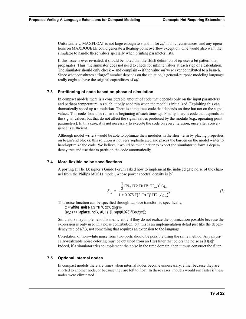
7.4 More flexible noise specifications

A posting at The Designer’s Guide Forum asked how to implement the induced gate noise of the chan-

nel from the Philips MOS11 model, whose power spectral density is [5]

(1)

This noise function can be specified through Laplace transforms, specifically,

x = white_noise(1/3*NT*Cox*Cox/gm);I(g,s) <+ laplace_nd(x, {0, 1}, {1, sqrt(0.075)*Cox/gm});

Simulators may implement this inefficiently if they do not realize the optimization possible because the

expression is only used in a noise contribution, but this is an implementation detail just like the depen-

dency tree of §7.3, not something that requires an extension to the language.

Correlation of non-white noise from two-ports should be possible using the same method. Any physi-

cally-realizable noise coloring must be obtained from an H(s) filter that colors the noise as |H(s)|2.

Indeed, if a simulator tries to implement the noise in the time domain, then it must construct the filter.

7.5 Optional internal nodes

In compact models there are times when internal nodes become unnecessary, either because they are

shorted to another node, or because they are left to float. In these cases, models would run faster if these

nodes were eliminated.

Sig

13--- NT 2 π f Cox⋅ ⋅ ⋅( )2 gm⁄⋅ ⋅

1 0.075 2 π f Cox⋅ ⋅ ⋅ gm⁄( )2⋅+----------------------------------------------------------------------------=

Proposed Verilog-A Language Extensions for Compact Modeling Extensions Requiring Further Research

20 of 22

This can be done by using optimizations to eliminate the nodes. First one would identify whether a node

were shorted to another node or terminal, or if it were completely floating. When such nodes were

found, they would not be created. In the case of shorted nodes, the name of the node being eliminated is

used as an alias for the node to which it is shorted.

Simulators must be responsible for checking whether a node is shorted or not, and whether that determi-

nation depends on a swept parameter.

Although model writers are perhaps accustomed to explicitly coding the short, they should not object to

being relieved of that burden. Tiburon-DA’s simulator is able to detect this condition automatically.

Thus, no extension is necessary.

7.6 Initial guess for Newton’s method

Some compact models recommend an initial value for branch voltages, such as those across the junc-

tions of a BJT or diode. These values sometimes give a better starting point for Newton’s method, which

is provably convergent only for starting points “close” in some sense to the solution.

Note that these initial guesses differ from nodeset values, which are already supported by the Verilog-

AMS language,. Nodeset values are enforced (typically through small resistors) for some number of

Newton iterations, but these initial guesses are only applied once for the first iteration.

Unfortunately, these initial values often depend on some knowledge of the external circuit. For example,

diode branches are often initialized at a positive bias to give a reasonable conductance; this is tremen-

dously helpful if the diode is driven by a current source and frequently helpful in other situations

because the linearized equation presented to the simulator tells it not to change the node potentials dras-

tically to change the current. However, if the diode is being held in reverse bias by voltage sources on its

terminals, then initializing the diode in forward bias is not helpful at all. It would be tedious for a model

author to attempt to write code to handle all the possible cases.

Further, the efficacy of these initial guesses is limited for large circuits. Hence, the subcommittee does

not recommend an extension to support this concept.

8.0 Extensions Requiring Further Research

The following items are more complicated, and the correct solution is not apparent. We expect a second

iteration through the compact modeling extensions to address these issues and others that were not

brought up in the subcommittee.

8.1 Inheritance

One might be interested in defining a set of models starting from a basic model and adding features. The

advanced models would inherit various things from the base model, such as structure, ports, parameters,

and then add further items. The idea is very much like the class inheritance of C++. Bell Labs is

reported to have used this sort of inheritance for a set of transistor models called “asim.” The simulator

was able to switch between model levels automatically when attempting to solve the circuit; it would

start with the base model and then work up to the complicated models.

The subcommittee feels that this extension would entail a great deal of effort on the part of the simulator

vendors, akin to moving their whole development system from C to C++. Further, the inheritance

method is not commonly used by authors of compact models.

Proposed Verilog-A Language Extensions for Compact Modeling References

21 of 22

8.2 Table models

Agilent is reportedly very interested in table models for devices. However, they did not communicate

their needs or suggestions to the subcommittee. Cadence’s Verilog-A implementation includes some

support for table models, and their approach has been forwarded to the Verilog-AMS committee for

consideration separate from these compact modeling extensions. We hope that these will be sufficient.

8.3 Frequency-domain descriptions

Many people have proposed adding frequency-domain modeling extensions to Verilog-A, but it is an

endeavor that is filled with risk. In addition, while appealing in concept, it is not very useful in practice

because there are very few models that can be easily described using formulas given in the frequency

domain that are also not easily given in the time domain, and the time domain formulas do not entail the

same degree of risk. Consider a few examples. Lumped components such as resistors, capacitors, and

inductors are easily described in the frequency domain, but they are also easily described in the time

domain, and time domain models are inherently more general as they can include nonlinear effects. This

leaves distributed components, which are nearly impossible to specify in the time-domain using only the

ddt and idt operators available in Verilog-A. However, in almost all cases, these models are also very

difficult to specify using formulas in the frequency domain. It is almost always easier to describe these

models in a tabular fashion in the frequency domain. So Verilog-A should provide a primitive instance

that is capable of reading industry standard s-parameter files, but that would not require supporting fre-

quency-domain extensions to the behavioral modeling capabilities in Verilog-A. There are a few models

that are both distributed, and so not easily described with time-domain models, and for which the fre-

quency domain formula is both simple and well known. Skin effect is perhaps the best known instance.

However, it is hard to think of many others. For these cases, we have two choices. One alternative is

simply to identify these cases and provide functions to implement the desired behavior (e.g., a skin

effect function). Simply implementing a function that provided a transfer function of Y(s) = sαX(s)

where α could be any number between –1 and 1 would go a long way in addressing the need for fre-

quency domain models.

If there were a strong desire to provide frequency domain modeling in Verilog-A, one would need to

address the causality issue. For frequency domain models to be causal, their real and imaginary parts

must be related in a complex and subtle way. The language must be designed in such a way that these

conditions are met, otherwise the models will not be compatible with time-domain simulators.

We believe that any extensions of this type should originate from the RF extensions subcommittee.

8.4 Asserts

Some have requested an assert capability that would generate a simulator error, not a user error mes-

sage, and allow checking/reporting of multiple assertion failures.

9.0 References

[1] Verilog-AMS Language Reference Manual, version 2.1, available from Accellera, www.accel-lera.com/.

[2] Ken Kundert. Automatic Model Compilation, An Idea Whose Time Has Come. www.designers-guide.com/Opinion, May 2002.

[3] Silvaco International support web page, www.silvaco.com/downloads/verilogADownloads.html

http://www.designers-guide.com/Opinion

http://www.designers-guide.com/Opinion

http://www.accellera.com/

http://www.accellera.com/

http://www.silvaco.com/downloads/verilogADownloads.html

Proposed Verilog-A Language Extensions for Compact Modeling References

22 of 22

[4] Laurent Lemaitre, Colin McAndrew, Steve Hamm. ADMS — Automatic Device Model Synthe-

sizer. IEEE Custom Integrated Circuits Conference, May 2002.

[5] R. van Langevelde. MOS Model 11. Nat.Lab. Unclassified Report NL-UR 2001/813. Available

from http://www.semiconductors.philips.com/Philips_Models/mos_models/model11/

[6] J.A. Barby, R. Guindi, "CircuitSim93: A circuit simulator benchmarking methodology case study",

Proc. IEEE Int. ASIC Conf., Rochester, NY, pp.531-535, Sep 1993.

extending verilog-a for compact modeling -...

Documents