Externalities and Bene�t Design in Health

Insurance

Amanda Starc

Kellogg School of Management, Northwestern University and NBER

Robert J. Town∗

University of Texas - Austin and NBER

October 2016

Abstract

We show that pro�t-maximizing insurers alter product design in the Medicare pre-

scription drug coverage market to account for underutilization by consumers. Using

policy induced variation in subsidies, we document that plans that cover all medical

expenses spend more on drugs than plans that are only responsible for prescription

drug spending, consistent with drug spending o�setting some medical costs. The e�ect

is driven by drugs that are likely to generate substantial o�sets. Our supply side model

con�rms that di�erential incentives across plans can explain this disparity. Counterfac-

tuals show that the externality created by stand-alone drug plans is $520 million per

year.

∗Kellogg School of Management, 2001 Sheridan Road, Evanston, IL and Department of Economics, TheUniversity of Texas at Austin, 2225 Speedway, Austin, TX. They gratefully acknowledge funding from theLeonard Davis Institute. Michael French, Matt Grennan, Ben Handel, Jonathan Ketcham, Kurt Lavetti,Maria Polyakova, Joshua Schwartzstein, Ashley Swanson, and participants at the American Health Eco-nomics Conference, FTC Microeconomics Conference, NBER Insurance Meetings, Kellogg Healthcare Mar-kets Conference, Wharton IO lunch, and Yale provided helpful comments. Emma Boswell Dean providedexcellent research assistance.

1

1 Introduction

Health insurance, while mitigating �nancial risk, can create a welfare loss from moral

hazard by lowering the price of medical services to consumers below marginal cost. Opti-

mal insurance contracts rely on cost sharing via deductibles, coinsurance and co-payments

to mitigate this welfare loss.1 However, there is also substantial evidence that consumers

reduce the utilization of cost e�ective care in the face of increased cost sharing (Manning

et al. (1987), Brot-Goldberg et al. (2015)). This can lead to ine�cient underutilization,

which we de�ne as foregoing treatments for which the societal bene�t exceeds the treatment

cost. Foregoing cost e�ective care in the present may lead to additional, more costly health

care consumption in the future, creating an externality. The extent of underutilization crit-

ically depends on how health insurers design their products in equilibrium. If insurers face

the �nancial consequences of ine�cient under-consumption, they have a clear incentive to

mitigate this underutilization through more generous bene�t design and other interventional

strategies. To the extent that insurers do not internalize and mitigate (and perhaps even

exploit) this underutilization, there are likely large societal and welfare consequences. Unlike

the large literature devoted to insurers' responses to moral hazard, little empirical analysis

examines insurers' incentives and equilibrium responses to ine�cient underutilization.2

In this paper, we empirically examine insurers' cost-side incentives to improve adherence

by altering plan characteristics such as coinsurance and copayments. We build a model of

consumer choice and endogenous insurer product design, and then leverage policy induced

variation in �rm incentives to estimate the cost of providing product �quality� in the form

of drug plan generosity. The model is used to calculate equilibrium product quality under

alternative policies and incentives. In our setting, the extent of underutilization of high

value health care services depends on insurer incentives, which, in turn, depend upon the

institutional and regulatory setting in which �rms compete.

We apply our model to detailed data from the Medicare Part D program. This institu-

tional setting provides an excellent opportunity to examine these issues as there is variation

across types of plans in the incentive to design bene�ts accounting for underutilization and

o�sets in medical expenditures generated by increased pharmaceutical utilization. Under the

1The optimal insurance design across multiple treatments depends on the sustainability or complementar-ity between di�erent medical treatments (Ellis, Jiang and Manning (2015); Goldman and Philipson (2007)).

2The notion that health insurance can correct for behavioral hazard dates at least to the �value-basedinsurance design� movement (Chernew, Rosen and Fendrick (2007)). There are case studies of the impactof these designs but no analysis of the incentives to implement these types of designs or their impact in themarket context. Lavetti and Simon (2014) consider the role of both selection and o�sets in driving formularydecisions. Our approach utilizes claims data, allowing us to show a causal e�ect on utilization in additionto plan design.

2

Medicare Part D program, there are (roughly) two types of drug plans: stand-alone prescrip-

tion drug plans (PDPs) and Medicare Advantage (MA-PD) plans. Stand-alone PDPs only

cover pharmaceutical expenditures while MA-PD cover both drug and medical expenditures.

These di�erences imply that these two types of plans face di�erent bene�t design incentives.

Stand-alone PDPs have an incentive to minimize drug expenditures, while MA-PD plans

have an incentive to minimize overall medical and drug expenditures taking into account

spillovers from drug consumption to medical care utilization.

We begin by performing a detailed, reduced form analysis of the causal relationship

between Part D plan enrollment and measures of drug adherence, costs and utilization.

Speci�cally, we examine the impact of PDP versus MA-PD enrollment on a number of

prescription drug consumption metrics using a large, detailed, representative sample of Part

D claims. These data capture every drug purchase occasion for a 10% random sample

of Medicare bene�ciaries. We also observe the bene�ciary demographics, their previous

purchase occasions, the speci�c drug(s) they purchased, the out-of-pocket cost of the drug(s)

to the consumer, the location of the purchase in the bene�t design (e.g. donut hole) and the

point-of-sale pharmacy price of each drug.

Causal inference is an obvious challenge in our setting. Medicare bene�ciaries may di�er-

entially select into MA-PD and PDP plans and plans may operate in markets with di�erent

demand and cost structures, leading to biased estimates if unaddressed. In order to iden-

tify e�ects of MA-PD enrollment, we exploit institutional discontinuities in the subsidies

for Medicare Advantage plans across counties. Speci�cally, we use a discontinuity in pay-

ment rates that increases payments for plans in Metropolitan Statistical Areas with more

than 250,000 people. In the subset of counties to the right of the discontinuity, the MA-PD

subsidy is exogenously more generous and the MA-PD enrollment rates are correspondingly

signi�cantly higher, allowing us to identify the causal e�ect of MA-PD enrollment.

We �nd that enrollment in MA-PD plan causally increases total enrollee drug expendi-

ture. MA-PD plans reduce consumer out-of-pocket costs and increase their own spending

relative to stand-alone PDP plans. The net e�ect is to increase overall drug consumption.

Importantly and consistent with our underlying explanation, the increase in utilization is

concentrated among drugs previously identi�ed by Chandra, Gruber and McKnight (2010)

to have large health consequences in the short-run. Furthermore, the e�ect is larger in plans

with higher enrollee retention, as would be predicted by Fang and Gavazza (2011), and

among enrollees with chronic conditions, as would be predicted by Chandra, Gruber and

McKnight (2010). Despite statistically similar drug prices across plans, MA-PD plans have

lower cost-sharing for consumers for identical products; this e�ect is especially large for drugs

used to treat chronic conditions, like asthma, diabetes, and high cholesterol. Our results are

3

robust to alternative speci�cations, controls for levels of FFS spending, and distortions due

to other institutional features of the market, including the low-income subsidy.

We then turn to specifying and estimating the structural parameters of an oligopoly model

of premium and bene�t design choice. The model recovers cost and demand side parameters,

allowing us to understand the economic rationale behind increased prescription drug bene�t

generosity in MA-PD plans. The model parameters imply that the increased generosity of

MA-PD plans is driven by insurer cost side incentives and cannot be rationalized by demand-

side considerations. In order to capture insurer incentives, we model both consumer choice

and insurer plan design. Importantly, our model allows for drug expenditures and preferences

to vary across consumers and captures the extent to which di�erences in generosity by plan

type can be rationalized by consumer demand. Consistent with other work (Abaluck and

Gruber (2011)), the demand side estimates imply that consumers undervalue plan generosity

when choosing plans. Because we �nd the demand responses to bene�t design are so modest,

MA-PD plans therefore increase drug plan generosity to reduce medical costs rather than

attract consumers.

We then use the model to measure the impact of plans internalizing the externalities

generated by drug o�sets. We �nd substantial bene�t externalities in MA-PD plans: a $1

increase in prescription drug spending reduces non-drug expenditure by approximately 20

cents.3 Our estimates directly account for or are robust to many institutional features of

the MA and Part D markets, including the bidding mechanism and distortions from the

low-income subsidy. Our model implies that if stand-alone PDPs are forced to account for

this externality in their premiums and bene�t design behavior, they would increase drug

spending by 13%. Based on these estimates, we �nd that stand-alone Part D plans impose

a $520 million externality on traditional Medicare each year. Therefore, the plan design and

medical management applied by MA-PD plans may increase welfare beyond what can be

obtained by traditional social insurance alone. In contrast to a large literature focused on

the dead-weight loss due to moral hazard, our paper shows when an externality is present

the optimal bene�t structure is more generous and insurers will internalize o�sets if incented

to do so.

Our paper contributes to several strains of the health insurance and industrial organiza-

tion literature. Our work expands on the recent literature examining insurer competition in

private Medicare markets (e.g. Decarolis, Polyakova and Ryan (2015); Curto et al. (2015));

more broadly, this paper contributes to a recent and growing literature on endogenous prod-

3This estimate aligns with previous work by Chandra, Gruber and McKnight (2010), who examine o�setsusing demand-side utilization. We cannot employ a similar strategy because we do not observe medicalclaims for enrollees in MA-PD plans.

4

uct design (see Fan (2013) as well as Crawford (2012) for a review).4

The paper is organized as follows. Section 2 describes the market and Section 3 presents

the reduced form estimations. Section 4 describes and estimates our model of �rm behavior.

Section 5 presents counterfactual exercises that put the magnitude of our e�ect in context,

and Section 6 concludes.

2 Medicare Part D and Medicare Advantage

Medicare provides health insurance to the elderly in the United States.5 Medicare Parts

A and B, enacted in 1965, cover inpatient, outpatient and limited nursing home services,

respectively. Medicare Advantage (Part C) and Part D are administered by private insur-

ers. Medicare Advantage is an alternative to traditional Medicare under Parts A and B.

Medicare Part D represented a large expansion of the program in 2006, as Medicare did not

originally cover prescription drugs. Prescription drugs not only represented a growing part

of uninsured expenditure, but increased drug spending may reduce other medical spending.

Private insurers in Medicare Advantage have an incentive to take this o�set into account; in

this paper, we focus on the behavior of these private plans relative to stand-alone PDPs.

Private insurance options have been available to Medicare enrollees since the 1970s. This

program has gone by a variety of names over time (see McGuire, Newhouse and Sinaiko

(2011) for a comprehensive history), but is currently known as Medicare Advantage. The

program's popularity has waxed and waned over time generally coinciding with the level of

federal reimbursement. As of 2009, the last year of our sample, 23% of Part D bene�ciaries

were enrolled in a Medicare Advantage plan. Enrollment rates have continued to grow

post-A�ordable Care Act (ACA).6 There is also signi�cant geographic heterogeneity in the

popularity of MA-PD plans. Across consumers within a market, MA may be more attractive

to middle and lower income as well as healthier bene�ciaries.

During our sample period, a senior eligible for Medicare had a number of private insurance

choices. They could opt out of traditional Medicare and into a Medicare Advantage plan. In

this scenario, the private Medicare Advantage insurer would be responsible for all medical

spending. By contrast, the senior could remain in traditional fee-for-service (FFS) Medicare

4Fan (2013) is the closest to our setting, as she explores continuous quality attributes. See also Draganska,Mazzeo and Seim (2009); Eizenberg (2014); Sweeting (2010); Wollman (2016). The paper also contributesto the empirical industrial organization literature examining �rm behavior when consumers are imperfectlyinformed or have non-standard preferences (Grubb and Osborne (2012); Grubb (2012, 2014); Handel (2013);Ellison (2006)).

5Medicare also provides health insurance coverage for the disabled and those with End Stage RenalDisease. We do not focus on those populations in this paper.

6During our time period, from 2007-2009, approximately 1 in 4 bene�ciaries was enrolled in a MA-PDplan.

5

and then choose to augment Medicare Parts A and B with a Part D plan. In this scenario,

the private Part D insurer would cover drug expenditure, while the Medicare program would

directly cover non-drug medical spending, including hospitalizations and physician services.

Due to its sheer size, the MA program is important from a policy perspective, and despite

its popularity among consumers, the MA program has always been controversial. There is

substantial debate about the level of spending in MA as compared to traditional Medicare;

cherry-picking by MA plans could lead to over payment by the federal government or skew

bene�t design to attract favorable risks (Brown et al. (2014); Carey (2015)). Furthermore,

a more recent literature argues that a substantial portion of the private gains from the MA

program accrue to insurers, though the exact magnitude is a matter of debate (see Cabral,

Geruso and Mahoney (2014); Curto et al. (2015); Duggan, Starc and Vabson (2015)). By

contrast, a number of papers highlight the potential for better medical management under

MA (Afendulis et al. (2011)). There is also evidence that the bene�ts of Medicare Advantage

may spillover to traditional Medicare bene�ciaries (Baicker, Chernew and Robbins (2013)).

The Part D program has been popular among both bene�ciaries and policymakers since

its introduction in 2006. Researchers have argued that Part D has lowered the price of drugs

by increasing insurer market power relative to drug manufacturers (Duggan and Scott Morton

(2010)); these potential e�ciencies, along with a shift toward generic drugs, have led to

program costs lower than forecasted when this bene�t was passed into law. The subsidy,

which covers 74.5% of the premium, is substantial and it is �nancially bene�cial for most

Medicare bene�ciaries to enroll in some form of drug coverage. The program requires insurers

to provide coverage at least as generous as the �standard bene�t.� The standard bene�t has

a very nonlinear structure. The deductible in 2009 was $295, followed by 25% cost sharing in

the initial coverage region (ICR) up to $2700 of expenditure, followed by the infamous donut

hole where the enrollee incurs the entire cost of drug expenditures and, �nally, catastrophic

coverage where the enrollee faces a 5% coinsurance rate. Coordination of care and innovation

in bene�t design could be especially important given the nonlinear and idiosyncratic structure

of the Part D standard bene�t.

However, the majority of plans in our sample eliminate the deductible, and nearly one

quarter of MA-PD plans had some form of donut coverage in 2006.7 The strict regulation of

Part D plans, covering both the �nancial details of plans and formularies, creates a minimum

standard for plans. In addition to providing coverage that is actuarially equivalent to the

standard bene�t, plans must cover all or substantially all drugs within six protected drugs

classes and two or more drugs in another 150 categories. However, �rms can design their

7By contrast, only 6% of PDP plans had donut coverage in 2006. The donut hole is being phased out asa part of the ACA. See Hoadley et al. (2014) for additional details.

6

plans within these limits and, potentially, increase the generosity of their plans. Part D

bene�ts are administered in both stand-alone PDP plans and Medicare Advantage MA-PD

plans. The set of PDP plans available depends on which of the thirty-four regions an enrollee

lives in, while the set of MA-PD plans available depends on the county of residence. Our

paper explores these two programs in tandem, noting that insurers have di�erential incentives

across plans: While Medicare Part D plans are simply minimizing drug expenditures, MA-PD

plans have an incentive to take total medical costs into account.

A long literature, including the RAND health insurance experiment (Manning et al.

(1987)), has shown that increased cost sharing causally leads to a reduction in the consump-

tion of medical services. Furthermore, reductions in consumption due to higher cost sharing

seem to a�ect both high- and low-value services. Underutilization is especially important if

there are drug o�sets; that is, if spending on drugs reduces spending on other medical ser-

vices. Numerous studies have documented the presence of drug o�sets in employer-sponsored

plans (Chandra, Gruber and McKnight (2010); Gaynor, Li and Vogt (2007)) and the Medi-

care Part D program (McWilliams, Zaslavsky and Huskamp (2011)). These o�sets of medical

care costs are viewed as important enough to be included in government budget forecasts

of health care expenditures. The Congressional Budget O�ce, surveying the literature, as-

sumes that a 1% increase in drug consumption reduces non-drug medical consumption by

0.2% (CBO (2012)). Cost sharing may lead to sub-optimal consumption due to discrepancies

between private willingness to pay and social marginal cost for a variety of reasons. There

may be asymmetric information about the value of treatment (Manning et al. (1987)), mis-

alignment of copays across multiple technologies (Ellis, Jiang and Manning (2015); Goldman

and Philipson (2007)), or underutilization may be �due to mistakes or behavior biases,� re-

ferred to in the literature as behavioral hazard (Baicker, Mullainathan and Schwartzstein

(2015)). Within the context of the Part D program, the behavioral bias most frequently

explored is myopia (Abaluck, Gruber and Swanson 2015, Dalton, Gowrisankaran and Town

2015).8

8Ex ante, consumers may be naive or sophisticated about the potential for underutilization due to infor-mation issues, behavioral biases, or both. A sophisticated consumer will demand an insurance contract thatcorrects for this underutilization of high-value services to the extent that they value reduced spending orimproved health, creating a market for value-based insurance designs (Ellison (2006); Chernew, Rosen andFendrick (2007)).In addition, there is substantial evidence that consumers have di�culty assessing the impact of di�erential

bene�t design on their drug consumption when selecting a plan. The average consumer has 18 MA-PD plansand 35 PDP plans from which to choose. This can potentially lead to substantial consumer confusion, asenrollees must compare potential out-of-pocket costs and premiums across a wide range of plans. Abaluckand Gruber (2011) document deviations from the predictions of a rational choice model and over-weighing ofplan premiums, while Ketcham et al. (2012) argue that consumers have learned over time. Potentially coun-teracting consumer learning is consumer inertia, which has been documented by Ho, Hogan and Scott Morton(2015).

7

2.1 Data

Our primary data source is the rich Medicare Part D prescription drug event data. We

observe every prescription �ll for the years 2006-2009 for a random 10% sample of all Medi-

care eligibles. For much of our analysis, we aggregate this data to the enrollee-year level. We

supplement this data with information on bene�ciary and plan characteristics and merge in

MA reimbursement levels and county and metropolitan demographic information.

We begin with 14,407,011 bene�ciary years for the period 2007 to 2009. Of those

bene�ciary-year combinations, we observe �lls in a stand-alone PDP or MA-PD plan for

7,597,476. We exclude any bene�ciaries who receive low-income subsidies and are subject

to lower cost sharing.9 This leaves us with 4,802,000 bene�ciary-year observations. We

then drop any enrollees for whom we do not have claims in 2006 so that we can control for

previous utilization, leaving us with 3,534,965 observations. We exclude those consumers

who spend over the catastrophic cap, as insurers are only responsible for their small fraction

spending on the margin; because o�sets are likely to be large for this group, our estimates

will be conservative.10 Finally, we have to drop a number of observations for which we do

not have complete plan or population information. This leaves us with a total of 3,019,197

observations.

Summary statistics of our sample are presented in Table 1. In the full sample, the av-

erage bene�ciary is 77 years old, 62% are female and 91% are white. Average total annual

expenditure is $1639, and the variance is nearly as large as the mean despite the lack of high

spenders in the analysis sample. In many speci�cations, we restrict attention to consumers

who live in counties with metro populations between 100,000 and 400,000. In column 2, we

present summary statistics for this sub-sample. Average total expenditure for this group is

very similar for the population as a whole at $1697 per enrollee per year. Finally, in the last

two columns, we compare the characteristics of enrollees above and below the 250,000 cuto�

that de�nes an urban county and translates into higher reimbursements. Due to our large

sample size, there are statistically signi�cant di�erences in the observable demographics and

utilization across these two groups, however, the magnitudes of the di�erences are economi-

cally insigni�cant. We do not observe non-prescription medical claims for MA enrollees and

an important goal of the structural analysis is to infer the level medical expenditures and

importantly the drug o�set from insurer plan design decisions.

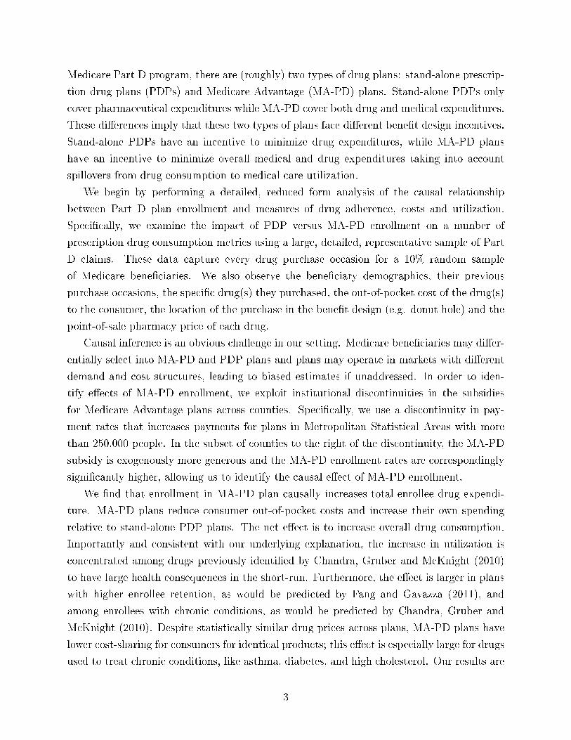
There is substantial heterogeneity in consumer spending, as highlighted in Figure 1. This

�gure plots a histogram of total spending in both MA-PD and standalone PDP plans in 2008.

9While we drop LIS enrollees for our main analysis, we run numerous robustness analyses to test thesensitivity of our �ndings to supply-side responses to the presence of the LIS population.

10See Table A.7 for additional analysis.

8

Table 1: Summary Statistics (Means and Standard Deviations)Metro Population Restrictions

None 100-400k 100-250k 251-400kTotal Drug Expenditure 1636.39 1697.33 1691.51 1704.51

[1288.74] [1284.98] [1284.65] [1285.36]Total Insurer Drug Expenditure 1026.79 1031.08 1021.48 1042.94

[826.31] [782.74] [775.54] [791.38]Enrollee Out-of-Pocket Costs 609.60 666.25 670.04 661.57

[664.60] [680.57] [682.11] [678.64]Total Rx Days Supply 1230.18 1262.58 1268.12 1255.75

[796.30] [785.66] [788.69] [781.86]% in MA 0.4048 0.2492 0.1962 0.3147

[0.4908] [0.4326] [.3971] [.4644]Age 76.9181 76.4850 76.5246 76.4361

[7.2325] [7.1025] [.0155] [.0171]% Female .6167 .6268 .6279 .6255

[.4862] [.4836] [.4834] [.4840]% White .9053 .9475 .9502 .9441

[.2929] [.2230] [.2175] [.2295]Observations 3,019,197 381,921 210,947 170,974

Notes: Table presents summary statistics describing mean consumer demographics,coverage, and utilization. The unit of observation is the enrollee-year. Sample isrestricted to consumers living in counties with populations in the range described inthe top row of the table. Standard deviations are in brackets.

9

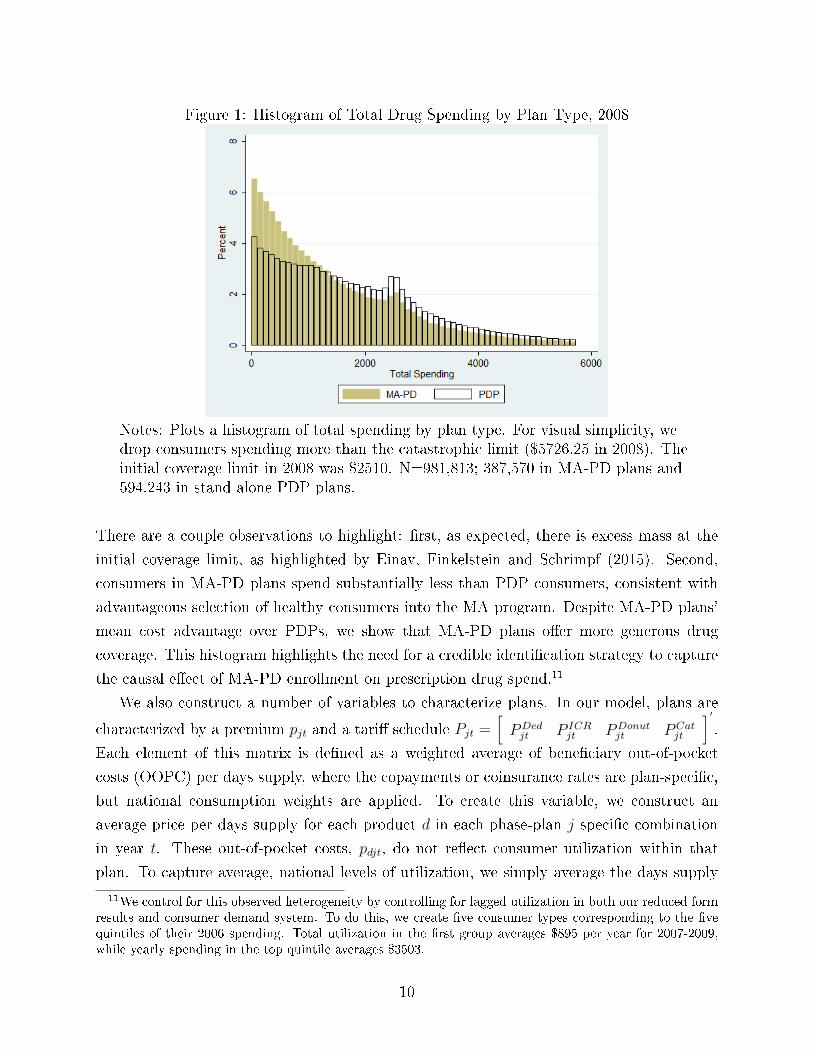
Figure 1: Histogram of Total Drug Spending by Plan Type, 2008

Notes: Plots a histogram of total spending by plan type. For visual simplicity, wedrop consumers spending more than the catastrophic limit ($5726.25 in 2008). Theinitial coverage limit in 2008 was $2510. N=981,813; 387,570 in MA-PD plans and594,243 in stand-alone PDP plans.

There are a couple observations to highlight: �rst, as expected, there is excess mass at the

initial coverage limit, as highlighted by Einav, Finkelstein and Schrimpf (2015). Second,

consumers in MA-PD plans spend substantially less than PDP consumers, consistent with

advantageous selection of healthy consumers into the MA program. Despite MA-PD plans'

mean cost advantage over PDPs, we show that MA-PD plans o�er more generous drug

coverage. This histogram highlights the need for a credible identi�cation strategy to capture

the causal e�ect of MA-PD enrollment on prescription drug spend.11

We also construct a number of variables to characterize plans. In our model, plans are

characterized by a premium pjt and a tari� schedule Pjt =[PDedjt P ICR

jt PDonutjt PCat

jt

]′.

Each element of this matrix is de�ned as a weighted average of bene�ciary out-of-pocket

costs (OOPC) per days supply, where the copayments or coinsurance rates are plan-speci�c,

but national consumption weights are applied. To create this variable, we construct an

average price per days supply for each product d in each phase-plan j speci�c combination

in year t. These out-of-pocket costs, pdjt, do not re�ect consumer utilization within that

plan. To capture average, national levels of utilization, we simply average the days supply

11We control for this observed heterogeneity by controlling for lagged utilization in both our reduced formresults and consumer demand system. To do this, we create �ve consumer types corresponding to the �vequintiles of their 2006 spending. Total utilization in the �rst group averages $895 per year for 2007-2009,while yearly spending in the top quintile averages $3503.

10

Table 2: Mean Plan CharacteristicsPDP MA

1(Deductible) .1912 .1655P ICR .5026 .4608∗∗∗

PDonut 1.93 1.71∗∗∗

Premium 23.16 12.77∗∗∗

Observations 381 1926

Notes: The unit of observation is the year-contract. P ICR and PDonut are calculatedfor a standardized population using claims data. Deductible and premiuminformation is taken from the Part D Plan Characteristics �le. Standard deviationsare in brackets. Statistically di�erent means at the 1% level denoted by ***.

by drug-year combination to create qdt. This weighting allows us to construct a measure of

consumer out-of-pocket costs that does not depend on the utilization of consumers within

the plan as:

P Phasejt =

∑d pdjtqdt.

This construction nests formulary inclusion, tiering, and coinsurance levels, but does not al-

low substitution if, for example, a particular drug was excluded from an alternative formulary.

While formularies are discrete, we create a continuous choice variable for tractability and

explore alternative constructions in robustness checks. Table 2 describes summary statistics

for each of these variables. Cost sharing is lower in MA-PD plans, especially in the donut

hole, where the average out-of-pocket cost per day supplied is 11% lower ($1.71 versus $1.93

for PDP plans). MA-PD plans also have lower cost sharing in the initial coverage phase (46

cents versus 50 cents) and lower premiums, due in part to generous reimbursement. These

summary statistics indicate that MA-PD plans are likely to be more generous and have

�atter cost sharing schedules than their PDP counterparts.

2.2 Identi�cation Strategy

Our goal is to estimate the causal impact of MA enrollment on total utilization, insurer,

and enrollee costs. However, a naive estimate will be contaminated by selection, as MA

enrollees are likely unobservably healthier than non-MA enrollees. Therefore, on average,

MA enrollees will have lower drug expenditure than their counterparts in stand-alone PDPs

for reasons other than plan design. This is likely to be true even once we control for a rich

set of individual characteristics.

Following a series of papers (Afendulis, Chernew and Kessler (2013); Cabral, Geruso

and Mahoney (2014); Duggan, Starc and Vabson (2015)), we rely on a statutory disconti-

nuity in MA-PD plan reimbursement to identify the causal impact of MA-PD enrollment.

11

For counties with relatively low fee-for-service (FFS) spending, payment is set equal to a

payment �oor. Beginning in 2003, di�erential �oors were set for urban and rural counties

� approximately two-thirds of counties are �oor counties. Higher reimbursement in urban

counties led to more plan entry and higher MA penetration rates (Duggan, Starc and Vab-

son (2015)). This variation in MA penetration rates appears driven by the di�erential MA

subsidies and is not correlated with individual health risk. Furthermore, because an urban

county is somewhat arbitrarily de�ned as one with 250,000 or more in metro population,

it is natural to focus the analysis on comparable counties near each side of the threshold.

Consumers in urban �oor counties close to the threshold are more likely to be enrolled in

MA-PD plans than consumers in observationally similar rural �oor counties just to the right

of the urban threshold.12 In our reduced form analysis, we use the county urban/rural status

as an instrument in a linear instrumental variable speci�cation; our empirical strategy is a

fuzzy regression discontinuity approach.

The identi�cation strategy hinges on the similarity of urban and rural �oor counties near

250,000 in metro population. We provide a battery of evidence of this balance in Table A.1;

using data from the Area Resource �les, we show that the �treated� and �control� counties

are similar in terms of demographic characteristics. In Figures A.3, A.4, A.5, and A.6,

we show binscatter plots con�rming that the covariates are not discontinuous across the

threshold. Previous research has shown that increased generosity may reduce MA premiums

and increases the amount of advertising (Cabral, Geruso and Mahoney (2014); Duggan,

Starc and Vabson (2015)). While none of these previous studies have found evidence of

a substantial increase in generosity, we will explore this possibility. Finally, unlike studies

examining the impact on providers (Afendulis et al. (2011)), we do not need to worry about

spillovers or general equilibrium e�ects, as we study insurer responses to the behavior of

individuals.

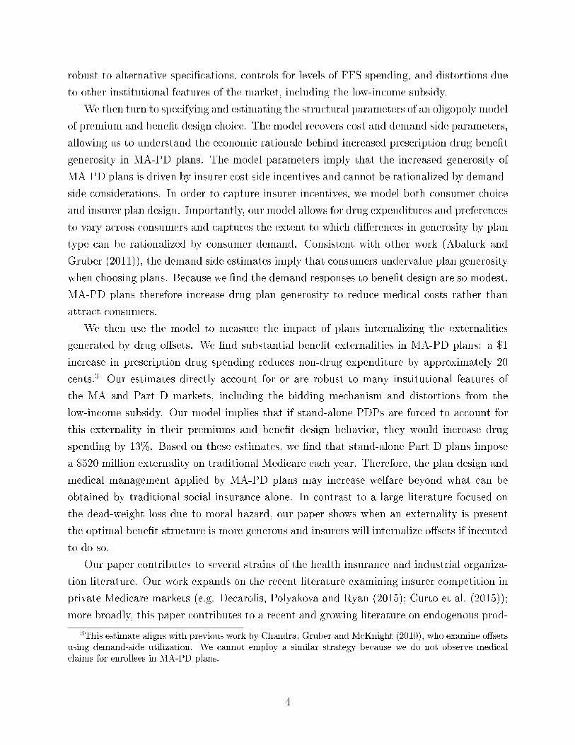
The variation we use in our IV speci�cations is highlighted in Figure 2, which plots the

probability of MA-PD enrollment as a function of population. This �gure depicts a binscatter

plot with twenty population bins. We control for consumer demographics, including risk

type, as well annual mean county-level FFS spending and plot the average probability of

MA-PD enrollment. We �t quadratic curves on either side of the 250,000 population cuto�.

We see a dramatic change in the probability of MA-PD enrollment just to the right of

the discontinuity. We implement our identi�cation strategy using an instrument variables

framework. Speci�cally, we estimate:

yitjm = X1mtβ1 +X2

itβ2 + β31(MA) + g(popmt) + µitj,

12We will also use urban status to predict the inside share of MA-PD plans in the plan choice models.

12

Figure 2: E�ect of Population on MA Enrollment

Notes: Plots a binscatter with twenty population bins. We drop counties with FFSspending above the urban �oor, and control for bene�ciary age, sex, race, 2006spending type, and county-level FFS spending. Lines represent a quadratic �t.

1(MA) = X1mtγ1 +X2

itγ2 + γ31(urbanmt) + g(popmt) + νitj,

where β3 is the coe�cient of interest, and X1mt and X

2it are vectors of market and individ-

ual speci�c covariates, respectively. In all speci�cations, we control �exibly for metro area

population. The dependent variables of interest, yitjm, are total drug spending, consumer

out-of-pocket costs, and insured costs. We hypothesize that insured spending is causally

higher in MA-PD plans, and consumer out-of-pocket costs lower. These relationships are

directly due to plan design on the part of insurers; the overall impact of these changes on

total expenditure is more ambiguous, as it depends on the size of the behavioral response,

but likely to be positive as well.

3 Reduced Form Analysis

To explore the impact of MA enrollment on utilization, we focus on the 2007-2009 time

period. In all speci�cations, we control for the consumer quintile of 2006 drug spending,

calculated at the national level. In our second and third speci�cations, we also control for

demographic characteristics (age, race, and gender), which capture part of the observable

risk. In our �nal, preferred set of speci�cations, we also control for historical county-level

FFS spending, which proxies for county level variation in of medical services, including drugs,

that might be driven by di�erences in patient preferences, medical care infrastructure and

the physician culture (see Finkelstein, Gentzkow and Williams (2016)).

Table 3 reports the results of OLS regressions of total expenditure, OOPC, and insurer

spending. These results are likely biased because of adverse selection into PDP plans � we

13

report them in order to provide a benchmark to the IV estimates. To make these results

directly comparable to the IV estimates, we focus the analysis on consumers living in counties

with associated metro populations between 100,000 and 400,000.13 In the bottom panel, we

examine the impact on total expenditure. The �rst column, which controls only for year

and the quintile of 2006 spending, shows that the average MA enrollee has lower drug

expenditures: total spending on drugs is $252 less than their counterparts in stand-alone

PDP plans. The average total expenditure for this sub-sample is $1697, indicating that MA

bene�ciaries have 15% lower drug spending than PDP enrollees. This lower expenditure is

associated with savings in the form of out-of-pocket costs to consumers (a reduction of $178)

and somewhat smaller reductions for insurers ($74 per enrollee per year). The next two

columns, which include demographic characteristics and county-level FFS spending, show

that the e�ect is not attenuated by the inclusion of additional controls.

In all of these speci�cations, we control for a rich set of observable characteristics. Clearly,

there may be selection conditional on unobserverbles as well as conditional on risk adjustment

(see Brown et al. (2014)). If there is advantageous selection of consumers into MA-PD plans,

our OLS estimates will con�ate the impact of plan design and the selection of consumers

across plans. In order to isolate the impact of plan design, we turn to our IV estimates.

3.1 Causal Estimates of the Impact of MA-PD Enrollment

We use changes in MA reimbursement as an instrument for MA coverage. In the �rst

panel of Table 3, we present the results of the �rst stage regressions that control for metro

population using a cubic spline with knots in increments of 100,000 starting at 150,000. In

all speci�cations, we �nd that Medicare eligibles in our dataset are 16-17% more likely to

enroll in a MA-PD plan if they live in an urban county. Given an average MA market share

of 25% within our sub-sample, this is a very large shift.14 By exploring what happens to

consumers who are exogenously shifted into MA-PD plans, we can isolate the impact of plan

design on utilization.

The second panel of Table 3 shows the estimated impact of MA enrollment on insurer

drug costs. Once we account for di�erential selection, MA-PD plans spend much more

on drugs than stand-alone PDPs. The MA enrollment estimate of $514 in column (4) is

approximately half of average insurer spending across all plans ($1031 per enrollee per year).

This estimate is more attenuated in the �nal column (albeit not statistically di�erent from

the estimates in column 4), which includes historical, county-level FFS costs as an additional

control. As noted above, this is our preferred speci�cation. Here the estimates indicate that

13Speci�cations with alternative bandwidths are available in Table A.4.14Furthermore, our instrument has a great deal of predictive power. The partial F-stat in the �nal

speci�cation is 509.02.

14

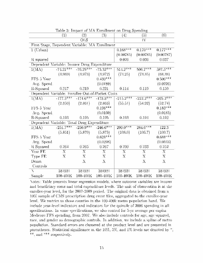
Table 3: Impact of MA Enrollment on Drug Spending(1) (2) (3) (4) (5) (6)

OLS IVFirst Stage, Dependent Variable: MA Enrollment1 (Urban) 0.168*** 0.170*** 0.177***

(0.00785) (0.00785) (0.00787)R-squared 0.026 0.036 0.037Dependent Variable: Insurer Drug Expenditure1(MA) -74.21*** -76.25*** -73.32*** 514.2*** 506.7*** 387.5***

(3.969) (3.973) (3.972) (74.25) (73.35) (68.38)FFS 5 Year 0.430*** 0.506***Avg. Spend (0.0189) (0.0226)R-Squared 0.217 0.219 0.221 0.114 0.119 0.159Dependent Variable: Enrollee Out-of-Pocket Costs1(MA) -177.5*** -174.6*** -173.3*** -215.2*** -222.2*** -265.2***

(2.850) (2.861) (2.863) (55.51) (54.92) (52.74)FFS 5 Year 0.198*** 0.183***Avg. Spend (0.0160) (0.0183)R-Squared 0.193 0.195 0.195 0.193 0.194 0.192Dependent Variable: Total Drug Expenditure1(MA) -251.7*** -250.9*** -246.6*** 299.0*** 284.6*** 122.3

(5.851) (5.870) (5.873) (108.0) (106.7) (100.7)FFS 5 Year 0.628*** 0.688***Avg. Spend (0.0298) (0.0343)R-Squared 0.264 0.265 0.267 0.230 0.233 0.252Year FE X X X X X XType FE X X X X X XDemo. X X X XControlsN 381921 381921 381921 381921 381921 381921Sample 100-400K 100-400K 100-400K 100-400K 100-400K 100-400K

Notes: Table presents linear regression models, where outcome variables are insurerand bene�ciary costs and total expenditure levels. The unit of observation is at theenrollee-year level, for the 2007-2009 period. The original data is obtained from a10% sample of CMS prescription drug event �les, aggregated to the enrollee-yearlevel. We restrict to those counties in the 100-400k metro population band. Weinclude year-level indicators and indicators for the quintile of 2006 spending in allspeci�cations. In some speci�cations, we also control for 5-yr average per capitaMedicare FFS spending, from 2007. We also include controls for age, age squared,race, and gender as demographic controls. In addition, we include a spline of metropopulation. Standard errors are clustered at the product level and are presented inparentheses. Statistical signi�cance at the 10%, 5%, and 1% levels are denoted by *,**, and *** respectively.

15

MA-PD plans spend $388 more per year than stand-alone PDPs for an equivalent enrollee.

As expected, historical FFS spending in�uences drug consumption: Finkelstein, Gentzkow

and Williams (2016) �nd that approximately half of all variation in spending is due to

place-speci�c supply factors. The following panels describe the impact of additional insurer

spending on consumers. The third panel shows that a consumer enrolled in MA can expect

to spend $265 less per year on drugs holding health risk constant. Consumer spending does

not fall one-for-one with the increase in insurer spending; this implies that the reduction

in average out-of-pocket costs for consumers increases utilization, as con�rmed in the �nal

panel. In our preferred estimates, the causal impact of MA enrollment is noisy, but implies

a $122 increase in drug utilization. On a base of $1697 of drug spending per year, this

represents a 7% increase in spending. Total utilization increases despite a drop in consumer

spending.

3.2 Mechanisms

We hypothesize that the underlying mechanism driving an increase in drug consumption

from MA enrollment is di�erences in MA-PD plan design intended to internalize the impact

of drug o�sets on non-drug medical spending. However, it is plausible that the di�erences

could be driven by di�erences in MA-PD plans themselves across the discontinuity. For

example, higher reimbursement may lead to more generous plans in urban �oor counties,

leading to higher utilization. We test this proposition in four additional sets of analyses and

�nd that the evidence does not support this interpretation, but is instead consistent with

insurer cost considerations driving the MA-PD pharmaceutical spending di�erences.15

First, there are no di�erences in average MA-PD plan characteristics across the urban

threshold. In this analysis, we restrict attention to only MA-PD plans and measure bene�t

generosity in terms of patient costs per day supplied. This measure, which captures copays

and coinsurance rates, can be thought of as the average cost of a pill to the consumer under

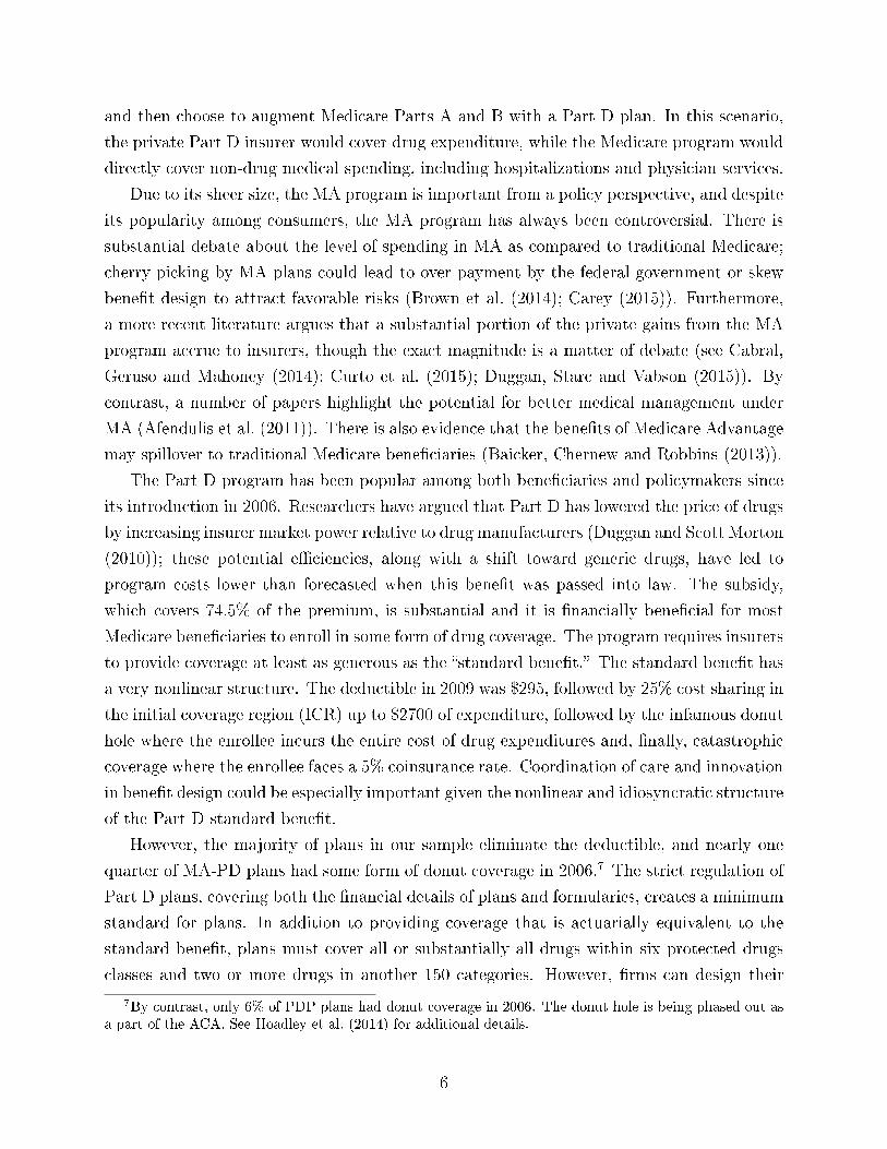
a given insurance plan.16 Figure 3 plots enrollee costs per day supplied as a function of

population. Consumers in MA-PD plans to the left of the 250,000 discontinuity face similar

drug costs as those consumers to the right of the discontinuity; the di�erence (two cents per

day higher or less than three percent) is not statistically signi�cant; the lower bound of the

15The reduction in OOPC to consumers of $265 per year represents 30% of the increased benchmark, whichis greater than the upper bound of pass-though estimates, as described in Cabral, Geruso and Mahoney(2014), and much higher than the estimates in Duggan, Starc and Vabson (2015) that cover the same timeperiod. In addition, while our structural model will incorporate increased subsidies, our model of plan choicewill show that increased generosity is not particularly salient to consumers, making changes in plan designunlikely unless they are driven by cost side o�sets.

16We note that this is a summary measure and abstracts from speci�c formulary and gap coverage decisions.While this measure abstracts from speci�c features of Part D plans, it captures a single dimensional measureof plan generosity.

16

95% con�dence interval allows us to reject decreases on more than 1.6 cents to the right of

the threshold. MA-PD plans do not o�er discontinuously more generous drug coverage in

urban counties.17 Therefore, our local average treatment e�ect measures the causal impact

of moving bene�ciaries from traditional FFS to MA plans, rather than re�ecting di�erences

in MA plans across the payment discontinuity. We also note the other factors, including

upcoding or di�erential plan networks, could a�ect utilization across the threshold. Table

A.2 presents the reduced form of our main IV speci�cations separately for the full sample and

MA-PD plans. These results con�rm that di�erences in MA-PD plans across the threshold

do not drive our main results.

Columns 1-3 of Table A.2 present OLS speci�cations where the coe�cient of interest is

on the dummy for being above the 250,000 population threshold (our excluded instrument).

As anticipated, the coe�cient is positive and signi�cant in the �rst panel (where the depen-

dent variable is insurer costs) and negative and signi�cant in the second panel (where the

dependent variable is consumer out-of-pocket costs). The net e�ect is positive. In columns

4-6, we restrict attention to consumers enrolled in MA-PD plans only and estimated the

same reduced form speci�cation. If our results were driven by greater generosity of MA

plans across the 250,000 threshold, we would expect a pattern similar to the full sample.

However, that is not what we see in the data; if anything, insurers in MA plans are spending

less on drugs as you cross the population threshold, though the di�erence is not statistically

signi�cant. Furthermore, we can reject the hypothesis that overall drug spending is higher

in urban counties. Therefore, we believe we are capturing the e�ect of moving consumers

from stand-alone PDPs to MA-PD plans rather than increased generosity of MA plans in

urban counties.

Second, we examine the impact of enrollee retention on the magnitude of the estimated

MA enrollment e�ect. If insurer cost considerations drive our results, plans with longer

average enrollee retention over our sample period should have larger MA e�ects than plans

with below average retention. If consumers are likely to remain with the same plans, insurers

have a greater incentive to invest in health bene�ts that will accrue over time (Fang and

Gavazza (2011)). We perform the analysis by splitting our sample by plan level retention

and restrict attention to above median retention plans.18 The results are in columns 1 - 3

17One could also be concerned that non-drug features of MA plans change discontinuously. In particular,if �rms bid below the higher benchmark, rebates may be higher in urban counties, leading to more generousmedical bene�ts. To the extent that drug and non-drug consumption are complements, this could bias ourresults. However, in Figure A.2, we show that rebates do not discontinuously increase across the discontinuity.In Table A.1, we also show balance in plan characteristics across counties above and below the threshold,with the exception of out-of-pocket medical costs, which are slightly lower in urban counties.

18Because these plans are larger, a substantial percentage of consumers are concentrated in these highretention plans, de�ned as having the highest percentage of consumers enrolled in 2006 continuously enrolled

17

of Table 4. MA enrollment increases insurer drug spending by $531 (versus $388 in the full

sample) and reduces enrollee OOPC costs by $274 (versus $265 in the full sample) in this

sub-sample. Although plan retention is possibly endogenous, they are broadly consistent

with the cost consideration hypothesis.

Figure 3: E�ect of Population on MA-PD Plan Drug Generosity

Notes: Plots a binscatter with �fty population bins using data from 2007. We dropcounties with FFS spending above the urban �oor, and control for bene�ciary age,sex, race, 2006 spending type, and county-level FFS spending. Lines represent alinear �t.

Third, we consider the impact of MA enrollment for enrollees taking medication for a

common, chronic health condition: hyperlipidemia. Hyperlipidemia (or high cholesterol) is

the elevation of lipid and lipid protein levels in the blood and is a risk factor for heart disease,

stroke and other vascular diseases. Adherence to hyperlipidemic medications meaningfully

reduces the likelihood of heart attack and stroke. Consistent with Chandra, Gruber and

McKnight (2010), which �nd that o�sets are larger among patients with chronic conditions,

we expect MA-PD plans to spend more on drugs like hyperlipidemics that target chronic

conditions. In columns 4-6 of Table 4, MA enrollment increases insurer drug spending by

$559 in the hyperlipidemic sub-sample. Even with a higher level of spending for this group

($2058 per enrollee per year), this represents a larger percentage increase in spending in MA

by insurers (27% versus 18% for the entire sample).19

Fourth, expanding on our results for hyperlipidemics, we show that the e�ect of MA

enrollment on utilization is driven entirely by drugs believed to have large o�sets a priori.

We explore the total bene�ciary level of utilization of �Category 1� drugs, as classi�ed by

through 2009.19The more pronounced increase in insurer spending also leads to higher overall utilization, though the

estimates are noisy. We further explore the e�ect on consumers in Figure 4.

18

Table 4: Impact of MA Enrollment on Drug Spending(1) (2) (3) (4) (5) (6)

Above Median Retention Plans HyperlipidemicsDependent Variable: Insurer Drug Expenditures1(MA) 710.0*** 706.2*** 531.2*** 718.6*** 729.2*** 559.1***

(92.85) (92.30) (83.47) (122.1) (122.6) (111.5)FFS 5 Year 0.522*** 0.621***Avg. Spend (0.0246) (0.0352)R-squared 0.037 0.042 0.114 0.188 0.114 0.119Dependent Variable: Enrollee Out-of-Pocket Costs1(MA) -192.5*** -202.0*** -273.9*** -203.4*** -193.6*** -259.7***

(68.43) (68.06) (64.29) (95.46) (95.51) (90.78)FFS 5 Year 0.214*** 0.241***Avg. Spend (0.0198) (0.0307)R-Squared 0.192 0.193 0.190 0.149 0.150 0.150Dependent Variable: Total Drug Expenditures1(MA) 517.5*** 504.2*** 257.3** 515.2*** 535.6*** 299.4*

(133.5) (132.6) (121.7) (177.1) (177.7) (163.9)FFS 5 Year 0.736*** 0.862***Avg. Spend (0.0370) (0.0541)R-Squared 0.199 0.203 0.238 0.133 0.132 0.172Year FE X X X X X XType FE X X X X X XDemo. X X X XControlsN 358,108 358,108 358,108 163,435 163,435 163,435Sample 100-400K 100-400K 100-400K 100-400K 100-400K 100-400K

Notes: Table presents parameter estimates and standard errors of the instrumentalvariable regression models, where outcome variables are insurer and bene�ciarycosts and total utilization levels. First-stage regressions are reported in the �rstpanel. The unit of observation is at the enrollee-year level, for the 2007-2009 period.The original data is obtained from a 10% sample of CMS prescription drug event�les, aggregated to the enrollee-year level. We restrict to those counties in the100-400k metro population band. We include year-level indicators and indicators forthe quintile of 2006 spending in all speci�cations. In some speci�cations, we alsocontrol for 5-yr average per capita Medicare FFS spending, from 2007. We alsoinclude controls for age, age squared, race, and gender as demographic controls. Inaddition, we include a spline of metro population. Standard errors are clustered atthe product level and are presented in parentheses. Statistical signi�cance at the10%, 5%, and 1% levels are denoted by *, **, and *** respectively.

19

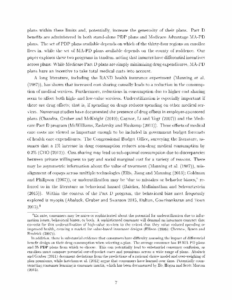
Figure 4: Spending by Class

Notes: This �gure presents the coe�cients and 95th percent con�dence intervalbands on MA-PD enrollment from three separate regressions. In the �rst, spendingon �Category 1� drugs, de�ned in the appendix, is the dependent variable. In thesecond, spending in the complement of this set is the dependent variable. In the�nal, overall drug spending is the dependent variable. All regressions control foryear �xed e�ects, consumer demographics, and county FFS spending. Standarderrors are clustered at the enrollee level.

Chandra, Gruber and McKnight (2010) and detailed in the appendix. If these drugs are not

taken, a serious event, such as a hospitalization, is likely to occur within the next six months.

By contrast to our previous results for those with hyperlipidemia, these speci�cations explore

the e�ect on a subset of consumption, rather than a subset of consumers.

Table 5 describes these results. About 40% of average expenditure ($648.11) is concen-

trated in these Category 1 drugs. Consistent with previous speci�cations, the OLS results

are biased downward due to advantageous selection into MA-PD plans. However, the IV

speci�cations in columns 3-6 show a consistent pattern: MA-PD enrollees consume propor-

tionally more of these �Category 1� drugs, due in large part to greater insurer expenditure.

MA-PD enrollment leads to an additional $156 in total spending on these drugs; on a base

of $648, this amounts to a 24% increase, versus 7% for total drug utilization. Put di�erently,

all of the increased total expenditure in MA-PD plans is concentrated in these large o�set

drugs.20 This can be seen in Figure 4, which plots the results overall, among the high o�set

drugs, and outside of the high o�set drugs. MA-PD plans do not spend more on drugs that

are unlikely to have large o�sets. We take these results, which describe heterogeneity across

plans, patients, and drugs, as additional evidence that our reduced form results capture

insurer incentives to mitigate ine�cient underutilization by consumers.

20Total expenditure in this category increases by $156, while overall total expenditure increases by $122.This also indicates a drop in consumption of drugs without large o�sets.

20

Table 5: Impact of MA Enrollment on Spending, Drugs with Large O�sets(1) (2) (3) (4) (5) (6)

OLS IVDependent Variable: Insurer Drug ExpendituresMean 401.16SD 512.61(MA) -18.63*** -18.30*** -17.52*** 223.5*** 229.6*** 190.8***

(3.118) (3.122) (3.124) (56.20) (55.66) (53.20)FFS 5 Year 0.126*** 0.156***Avg. Spend (0.0150) (0.0170)Mean 0.046 0.047 0.047 0.005 0.005 0.018Dependent Variable: Enrollee Out-of-Pocket CostsMean 246.96SD 379.181(MA) -58.56*** -56.57*** -56.42*** -27.68 -27.73 -34.43

(1.848) (1.849) (1.848) (37.24) (37.24) (35.40)FFS 5 Year 0.0238** 0.0270**Avg. Spend (0.0103) (0.0116)R-Squared 0.064 0.065 0.065 0.063 0.064 0.065Dependent Variable: Total Drug ExpendituresMean 648.11SD 802.671(MA) -77.19*** -74.86*** -73.94*** 195.8** 201.9** 156.4*

(4.497) (4.505) (4.507) (84.52) (83.64) (80.17)FFS 5 Year 0.150*** 0.183***Avg. Spend (0.0230) (0.0260)R-Squared 0.064 0.065 0.066 0.043 0.044 0.051Year FE X X X X X XType FE X X X X X XDemo. X X X XControlsN 322,066 322,066 322,066 322,066 322,066 322,066

Notes: Table presents parameter estimates and standard errors of the instrumentalvariable regression models, where outcome variables are insurer and bene�ciarycosts and total utilization levels. The unit of observation is at the enrollee-yearlevel, for the 2007-2009 period. We restrict to those counties in the 100-400k metropopulation band. We include year-level indicators and indicators for the quintile of2006 spending in all speci�cations. We include controls for age, age squared, race,and gender as demographic controls. In addition, we include a spline of metropopulation. Standard errors are clustered at the product level and are presented inparentheses. Statistical signi�cance at the 10%, 5%, and 1% levels are denoted by *,**, and *** respectively.

21

Finally, we explore the relationship between MA-PD enrollment and out-of-pocket drug

costs to consumers.21 These tests do not rely on the exclusion restriction from our IV

speci�cations as the level of observation is the drug �ll. Furthermore, they are robust to other

threats to our identi�cation strategy, including increased non-drug generosity among MA-

PD plans in non-urban counties and upcoding by MA-PD plans.22 We control for national

drug code (NDC) �xed e�ects, which capture all of the variation related to the detailed

product and package (ie 20mg of Lipitor). Therefore, this analysis is complementary to the

results in Table 3 as it relies on a di�erent source of variation to identify the MA-PD e�ect.

Table 6 presents the results of this exercise. In the �rst speci�cation for each dependent

variable, we include year �xed e�ects. In the second, we control for the year and the phase

of the prescription drug bene�t, as insurers can alter consumer cost sharing given the bene�t

structure or the bene�t structure itself. We examine the impact of MA-PD plans on the

log consumer out-of-pocket costs and the likelihood of 90-day �lls, noting that there are not

statistical di�erences in point-of-sale prices across plan type. The results show a pattern

consistent with the main enrollee-year results. For MA-PD plans, consumers face a cost that

is 5-7.5% lower per day supplied, holding the drug (NDC) constant. For identical drugs,

consumers in MA-PD plans pay less at the point-of-sale, and this e�ect is meaningful.23

In Figure 5, we show that the cost-sharing results are larger for speci�c drug classes

targeted by value-based insurance designs in the commercial insurance market (Chernew,

Rosen and Fendrick (2007); Gowrisankaran et al. (2013)). Speci�cally, we �nd statistically

larger e�ects among drugs used to treat diabetes, asthma, and hyperlipidemia (high choles-

terol). The results for hypertension (high blood pressure) are more mixed. However, in

Figure A.1, we show that this is due to heterogeneity across types of hypertensives. For the

21In unreported regressions, we con�rm two additional pieces of information. First, total cost per daysupplied for a given drug is equal across plans; negotiated prices are not systematically higher or lowerfor MA-PD plans. Second, individual contracts do not o�er more generous bene�ts in urban counties. Ifanything, the average consumer out-of-pocket cost per days supply is slightly higher to the right of the250,000 threshold.

22Furthermore, we note that drug consumption is not included in the risk adjustment scheme, and bothupcoding and risk selection are less likely to be problematic in our setting (Carey (2015)).

23Finally, in the second panel, we see some evidence that consumers in MA-PD plans are more likely to �ll90-day prescriptions, which likely contributes to increased adherence; the estimates imply that 1.4% moreprescriptions are 90-day �lls under MA-PD plans, making the e�ect small, but still indicative of di�erentialstrategies by plan type. In unreported regressions, we �nd that the OOPC cost for hyperlipidemia drugs inMA-PD plans is 12-15% lower than in PDP plans, consistent with lower out-of-pocket costs for drugs forchronic conditions. Finally, in Figure 4, we restrict to drugs labeled as �Category 1� by Chandra, Gruberand McKnight (2010) and estimate the causal e�ect of MA-PD enrollment separately by class. If these drugsare not taken, a serious event, such as a hospitalization, is likely to occur within the next six months. Onaverage, these drugs are cheaper in MA-PD plans, consistent with an incentive to minimize overall drugcosts. This is not true for all categories; as pointed out by Lavetti and Simon (2014), selection may a�ectplan design as well. In the structural model, we will allow for di�erential incentives that incorporate botho�sets and selection.

22

Table 6: Mechanisms(1) (2)

Outcome: Logged OOPC/Day1(MA) -0.075*** -0.049***

(0.0033) (0.0035)Constant -1.028*** -2.219***

(0.0024) (0.0058)Observations 124,801,603 124,801,603Adjusted R-Squared 0.607 0.673

Outcome: 1(90 Day)1(MA) 0.001*** 0.001***

(0.0009) (0.0009)Constant 0.108*** 0.103***

(0.0007) (0.0006)Observations 157,091,471 157,091,471Adjusted R-Squared 0.096 0.096Product Fixed E�ects X XPhase Fixed E�ects X

Notes: Table presents linear regression models, where outcome variables are asdescribed in each panel. The unit of observation is at the �ll level, for the 2007-2009period. The original data is obtained from a 10% sample of CMS prescription drugevent �les. We include year-level indicators and product �xed e�ects in allspeci�cations. In some speci�cations, we also control the phase of the standard PartD bene�t. Standard errors are clustered at the plan-product level.

23

Figure 5: Out-of-Pocket Cost E�ects by Drug Class

Notes: This �gure plots the mean di�erences and standard error bands inout-of-pocket costs by plan type for each of four drug classes. Diabetes drugsinclude glucose monitoring agents, insulins, alpha-glucosidase inhibitors,meglitinides, amylin analogs, sulfonylureas, incretin mimetics, SGLT-2 inhibitors,dipeptidyl peptidase 4 inhibitors, non-sulfonylureas (metformin), thiazolidinedionesand antidiabetic combination therapies. Asthma medications include inhaledcorticosteroids, anticholinergic bronchodilators, leukotriene modi�ers,methylxanthines, and antiasthmatic combination therapies. Hypertension drugsinclude beta blockers, ACE inhibitors, angiotensin II receptor antagonists, renininhibitors, antiadrenergic agents (centrally & peripherally acting), alpha-adrenergicblockers, aldosterone receptor antagonists, vasodilators, calcium channel blockersand anti-hypertensive combination therapies. Hyperlipidemia drugs include statins,cholesterol absorption inhibitors, bile acid sequestrants, �bric acid derivatives, andantihyperlipidemic combination therapies. Standard errors are clustered at theplan-product level.

most cost-e�ective, recommended initial therapy (non-beta blockers)24, the e�ect is in the

expected direction. Furthermore, in Table A.3, we provide a falsi�cation exercise, showing

that we do not get the same result if we restrict attention to protected drug classes, in which

stringent regulation requires generous coverage by stand-alone plans. In summary, MA-PD

plans have lower out-of-pocket costs for identical drugs, and this e�ect is especially large for

high value drugs.

In the Appendix, we perform a number of robustness checks. In Table A.4, we restrict

our sample to just consumers living in counties with metro populations of 200,000-300,000.

Here, our results are larger in magnitude. Also in Table A.4, we restrict our sample to only

low FFS counties, where the �oor is more likely to bind. Again, the estimates are larger

in magnitude, though also noisier. The results are qualitatively similar in logs and levels;

24NICE (2011)

24

this makes sense, as our results exclude outliers. In the �nal three columns of Table A.4, we

include enrollees with no �lls and expenditure above the catastrophic limit. The results are

again similar, though noisy. We show that our results are robust to alternative population

controls in Table A.5. We control for linear, quadratic, cubic, and quartic functions of metro

population, in addition to linear and cubic splines with knots at the discontinuity of 250,00;

none of the estimates are statistically di�erent from our preferred estimates as shown in

column 3 of Table 4. Table A.6 shows that our results are not sensitive to the exclusion of

bene�ciaries enrolled in plans that may be distorted due to the low-income subsidy discussed

below. Finally, in Table A.7 we show that our qualitative results are not sensitive to the

inclusion of bene�ciaries exceed the catastrophic cap, though including these bene�ciaries

greatly increases the variance and skew of our estimates. Finally, Table 8 shows that our

results are not sensitive to the exclusion of bene�ciaries not enrolled in 2006 or the inclusion

of region �xed e�ects.

Taken together, our reduced form results show a consistent pattern. MA-PD plans are

designed in ways that reduce consumer cost sharing and, to a lesser extent, increase drug

utilization. The e�ect is concentrated in drugs likely to generate large o�sets. An identical

consumer will pay less for a higher quantity of drugs in a MA-PD plan than in a standalone

PDP plan. We next examine the incentives MA carriers face to internalize o�sets using a

model of insurer plan design.

4 Model of Premium Setting and Bene�t Design

4.1 Overview

In this Section, we describe our model of equilibrium insurer plan design and outline

our estimation strategy. We estimate the structural parameters of this model in order to 1)

decompose demand and cost side rationales for MA-PD plans to o�er more generous drug

coverage; 2) provide estimates of the implied externality of increased drug coverage and the

magnitude of the drug o�set; and 3) perform policy counterfactuals. Our model is simple

enough to be tractable yet rich enough to capture the complexity of equilibrium insurer

behavior when setting premiums and bene�ts. In this framework, insurers have three choice

variables for each contract j: premium, pj, and the average out-of-pocket cost per days

supply in both the initial coverage phase and in the donut hole, Pj =[P ICRj , PDonut

j

]′.

Firms maximize pro�ts, which depend on their own premiums, subsidies and costs (which

endogenously depend on the enrollee risk pool) as well as the equilibrium decisions of their

25

competitors. Insurer drug costs, as well as market shares, are a function of the generosity of

the plan. We begin by describing endogenous plan design for a stand-alone prescription drug

plan and then expand the analysis to take into account di�erential incentives faced by MA-

PD plans. Consider the following simple model, in which variable pro�ts for a stand-alone

PDP are given by (omitting sub- and superscripts):

Π =(p+ zD − c(P )

)sB,

where p is the premium, z is the federal subsidy, c is the cost to the insurer, s is the

market share and B is the size of the Medicare population. This implies the standard �rst

order condition with respect to premiums and the following �rst order conditions product

characteristics:

(p+ z − c)∂s

∂P Phase+

∂c

∂P Phases = 0 for P ICR, PDonut.

Medicare Advantage plans face a di�erent set of incentives than stand-alone PDP plans.

Consider the choice to increase the generosity of a prescription drug plan. The PDP knows

that this will directly increase costs, as they bear a higher percentage of a �xed drug expendi-

ture. In addition, higher generosity plans may attract sicker patients and induce consumers

to spend more � the adverse selection and moral hazard e�ects, respectively. MA-PD plans

will also take these factors into account. In addition, a MA-PD plan must consider the

impact that drug expenditure has on overall medical expenditure. If there are drug o�sets,

increased drug expenditures lead to reduced (non-drug) medical expenditures. The average

total costs for a MA-PD are the sum of drug and (non-drug) medical costs: c = cD + cM .

MA-PD plans will di�er from PDPs in their cost sharing arrangements because their �rst

order conditions di�er with respect to one key term: ∂cM

∂PPhase .25 This is the object we want

to estimate: in the presence of drug o�sets, this term will be non-zero.

4.2 Empirical Implementation

There are a number of institutional complexities of the Part D and Medicare Advantage

programs that a�ect the mapping from insurer strategies to pro�ts and thus require mod-

i�cation the above illustrative model for estimation. Speci�cally, we account for the CMS

bidding mechanism, the presence of the low-income subsidy population, risk corridors, risk

adjustment and selection conditional on risk adjustment.

Insurers do not set premiums directly but rather submit a �bid� for both drug and non-

drug coverage. If the bid is above a benchmark amount, the consumer pays the di�erence

25That is, ∂c∂PPhase = ∂cD

∂PPhase for standalone PDPs and ∂c∂PPhase = ∂cD

∂PPhase + ∂cM

∂PPhase for MA-PD plans.

26

between the bid and the benchmark. If the bid is below the benchmark amount, which is

common for MA-PD plans, insurers must devote part of the di�erence between the bid and

the benchmark to providing more generous bene�ts.26 Following Decarolis, Polyakova and

Ryan (2015), we write ex-post pro�ts for stand-alone PDPs as a function of the bids, b, of

the �rm and other �rms in the market:

πPDPj (bj; b−j) = ΓPDP

∑i∈Aj

(pj(b̄; ri) + zDi (b̄; bj) − cDij (pj, ri, Pj)

) ,where Γ is a function that adjusts for ex-post risk corridor transfers and pj is the premium of

policy j, which depends on the entire vector of bids. In addition, zD is the (individual speci�c,

risk adjusted) subsidy, and cDij represents individual speci�c costs, which are a function of

the individual's risk score ri and plan characteristics, Pjt. Aj represents the set of consumers

who purchase good j which yields share sj. We separate out the individual component of

costs and risk adjusted payments ηij, letting HDj (Pj, pj) =

∑i∈Aj

ηij (Pj, pj) and summing

over markets m:

πPDPj (bj; b−j) =

∑m

ΓPDP[pj(b̄; bj) + zD(b̄) − cDj (pj, r̄, Pj) +HD

j (Pj, pj)]sjmBm.

The plan chooses their bid and cost sharing parameters Pj to maximize pro�t subject to an

actuarial equivalence (minimum generosity) requirement P :

maxbj ,Pj

πPDPj (bj; b−j)

s.t. Pj ≥ P .

The pro�t function for Medicare Advantage plans is similar, though there is an additional

(risk adjusted) payment for medical costs, zM .27 We write:

πMAj (bj; b−j) =

∑m

ΓMA[p+ zD − cDj +Hj (Pj, pj) + bMj + zM − cMj +HM

j (Pj, pj)]sjmBm,

26Previous research (Stockley et al. (2014)) indicates that consumers primarily respond to premiums, so wemodel the e�ect of the premium implied by an insurer's bid and account for subsidies in the pro�t equation.We explore the e�ect of rebates, which are positive for approximately 5-10% of plans (Stockley et al. (2014))in Figure A.2 and Table A.1.

27There are separate subsidies for the non-drug component of MA-PD plans that vary at the market level;we incorporate these explicitly. Therefore, higher generosity due to more generous subsidies will not implyo�sets. We abstract from MA rebates, which should increase the value of plans.

27

where the M superscripts re�ect medical (�Part C�) bids and costs, respectively, and

bMj is equal to the premium plus any rebates. Similar to stand-alone PDPs, MA-PD plans

must submit bids for medical coverage, incur costs that depend on individual and plan

characteristics, and receive risk adjusted subsidies. Because MA subsidies were generous

during our time period, some plans have zero premiums; these plans may include �rebates�

to consumers, which can be used to provide additional services or reduce Part B premiums,

which are required even for consumers in MA plans. We include these net premium reductions

directly in the de�nition of bM .28

This formulation of �rm pro�ts captures the bidding mechanism, risk corridors, and risk

adjustment. In order to address potential selection conditional on risk adjustment with re-

spect to plan characteristics, including cost sharing and premiums, we allow for preferences

and drug costs to vary �exibly by consumer type (de�ned as quintiles of the 2006 drug spend-

ing distribution). Therefore, Hj (Pj, pj) =∑

q∈j ηqj (Pj, pj), where q represents quintiles; if

a plan becomes more generous or sets a higher premium and that disproportionately at-

tracts higher cost enrollees, this will be re�ected (through a greater weighting of higher cost

quintiles) in Hj (Pj, pj) and∂Hj(Pj ,pj)

∂Pj.29 Conditional on consumer type, we assume constant

expected marginal costs. Our results are robust to this assumption as allowing for more

heterogeneity by de�ning �ner consumer types (for example, deciles of 2006 spending, or

conditioning on demographics) yield similar results. We do not need to impose an assump-

tion of optimal pricing for PDP plans; we will never use the �rst-order condition with respect

to drug premiums, though we will utilize the optimality of MA non-drug premiums to infer

costs (similar to Curto et al. (2015)) and will allow �rms to reprice plans in counterfactual

exercises.

This is especially important as previous research has highlighted that the presence of the

LIS subsidy can distort plan bidding incentives (Decarolis (2015); Decarolis, Polyakova and

Ryan (2015)). We explore the robustness of our results to the inclusion of plans that may

be distorted by the LIS subsidy in Section 4.5. In addition, while we collapse the variation

in formulary design into average consumer out-of-pocket costs per days supply, insurers also

design formularies along with coinsurance and copayment rates; we focus on this measure

of consumer costs in each phase of the standard bene�t, as directly modeling formulary

placement of every drug is computationally unfeasible. We assume that plans do not take

account of their impact on the benchmark when submitting bids. Given the large number of

plans, we believe this is a reasonable assumption. Because of data limitations (CMS prevents

28Finally, we can allow the value of the rebate to be reduced by 25% in accordance with CMS biddingrules. Table 11 shows that this will not a�ect our estimates of the key parameters of interest.

29We also allow changes in premiums to alter the risk pool the �rm attracts through∂Hj(Pj ,pj)

∂pj.

28

the identi�cation of speci�c plans beyond an encrypted ID in the PDE �les), insurers are

assumed to set optimal strategies ignoring cross-elasticities between plans in di�erent sectors

(for example, the increasing the bid of Humana's PDP plan decreases the enrollment of

Humana's MA plan). Below, we show that this elasticity is small and thus any bias from

this restriction is also small. Following a number of papers (Lustig (2010); Nosal (2011)),

we model �rm decisions at the contract level averaging across plan characteristics within a

contract.30 In Section 4.5, we test the robustness of our estimates to these assumptions.

4.3 Plan Choice

We �exibly model insurance demand using a nested logit model that allows for enrollee

heterogeneity in preference parameters by estimating the parameters by enrollee expenditure

type. A consumer's choice sets de�ned at the county-level and a product is a county speci�c

contract.31 Beyond these product characteristics, which can vary at the market level, we

use product �xed e�ects (which di�er by enrollee type) to capture invariant features of plan

quality, including relative non-drug premiums for MA-PD plans.

Consumers have preferences over plans, premiums, and out-of-pocket costs. This requires

constructing a function that relates PPhasejt (an insurer choice variable) to out-of-pocket costs (the

variable enrollee care about) for each phase. Given a vector of PPhasejt , we can create counter-

factual out-of-pocket costs given constant consumption (days supply) for consumer i with

30We do this for two reasons: �rst, we want to be conservative rather than introducing additional (po-tentially correlated) observations when computing standard errors. Second, drug prices are likely to benegotiated nationally rather than by plan ID within a contract, and this will a�ect the within contract priceindex we estimate.

31While Part D insurers have identical o�erings within the large 34 PDP regions, MA-PD plans canchoose which counties to enter within a given region. Following a number of papers, symmetric with theplan decision assumption discussed above, a MA-PD product is de�ned as a unique contract ID. The keyproduct characteristics from the consumer's perspective are the premium attributed to drug coverage, andout-of-pocket costs, as described above. If there is more than one plan within a contract, we use the productcharacteristics of the lowest numbered plan among MA-PD plan. Similarly, a stand-alone PDP plan is de�nedas a contract ID-county combination for the purposes of demand estimate; we average characteristics within acounty and the individual's out-of-pocket costs are based on their market. Assuming one plan ID per countywithin a contract, this is equivalent to de�ning the product at the contract ID-plan ID combination. Wedo not directly model the impact of non-drug premiums in MA-PD plans. Many plans have zero premiums,and some rebate a portion of the Part B premium, reducing salience to consumers and making measurementdi�cult.

29

consumption (days supplied) d as:

OOPCijt =

PDedjt (d)

if Rjtd < DED

P ICRjt

(d− DED

R

)+DED

if Rjtd ≥ DEDandRjtd < ICL

PDonutjt

(d− ICL

Rjt

)+DED + γICR(ICL−DED)

if Rjtd ≥ ICLandRjtd < CAT

PCatjt

(d− CAT

Rjt

)+DED + γICR(ICL−DED) + γDonut(CAT − ICL)

if Rjtd ≥ CAT,

,

where d is the days supplied, γ represents the average coinsurance in each phase, R is the

retail price, and DED, ICL, and CAT represent the deductible, initial coverage limit, and

catastrophic cap, respectively.

Following the reduced form analysis, we divide the sample into �ve �types� of consumers

based on quintiles of 2006 spending. In each quintile q, consumer utility for plan j (which

can be either a PDP or a MA-PD plan) in market m at time t is given by:

uqjtm = Xjβq − αp,qjtpjtm − αP,qjtOOPCijt + ξqjmt + (1 − σ)εijtm,

where Xj is a matrix of plan �xed e�ects, such that plan utility is allowed to vary with

consumer type, pjtm is the premium, OOPCqjt = f(P ICRjt , PDonut

jt ) is a function of the average

prices per days supply, and ξqjtm is the unobserved product characteristics.

Our speci�cation allows for consumer heterogeneity in preferences by including �exible

plan �xed e�ects that can vary by consumer type, which implicitly allows for di�erential

selection into plans based on consumer type.32 These speci�cations re�ect a few additional

modeling choices. First, while we allow plan unobserved quality, premium and out-of-pocket

cost coe�cients, and the dissimilarity term to vary by consumer type, there is no other

source of unobserved consumer heterogeneity in the model. In addition, we do not allow

for behavioral responses to average costs per days supply to factor into the out-of-pocket

cost calculation. Put di�erently, there is no selection on moral hazard and the relationship

between P ICRjt , PDonut

jt , and OOPCjt is purely mechanical. The derivative of shares with

respect to any element of the tari� vector is given by∑

q∂sqjtm

∂OOPCqjtm

∂OOPCqjtm

∂PPhasejtm

.

We estimate the parameters of the model separately for each quintile type using the

32We assume perfect risk adjustment conditional on type, but the cost to the insurer is allowed to varyacross quintiles. Our model does not explicitly accommodate selection with respect to formulary design(Carey (2015); Lavetti and Simon (2014)).

30

Berry (1994) speci�cation. We aggregate to the quintile-plan level while still estimating a

speci�cation �exible enough to account for substantial heterogeneity in consumer preferences.

In order to capture �rm incentives, we need to identify the causal impact of premiums and

out-of-pocket costs. The presence of unobserved quality, ξqjmt, makes this challenging. We

take a two-pronged approach. First, we include product �xed e�ects, so this unobserved

product characteristic is the deviation from the plan mean for the quintile in question.

Second, we instrument for the premium, out-of-pocket cost, and inside share. Following the

logic of the reduced form identi�cation strategy, the instrument for the inside share is the

urban dummy interacted with an MA dummy, which captures the fact that MA-PD plans

are more popular in urban counties. For both the premium and out-of-pocket costs, we

use Hausman style instruments: the average premiums and out-of-pocket costs in all other

markets. These instruments are commonly used in this setting (e.g. Decarolis, Polyakova

and Ryan (2015)) and capture common cost shocks as well as correcting for any measurement

error in our measure of out-of-pocket (drug) costs.

4.3.1 Demand Parameter Estimates

The results of the IV speci�cations for each of the �ve consumer groups are in Table 7.

Interestingly, once we allow consumer preferences for individual plans to vary across drug

spending quintiles, we do not �nd much heterogeneity in the premium or OOPC coe�-

cients. While the premium coe�cient is negative and signi�cant in all speci�cations, sicker

consumers are slightly less price sensitive than healthier consumers, consistent with adverse

selection with respect to generosity. Second, the out-of-pocket cost coe�cient is meaningfully

smaller in magnitude than the premium coe�cient, consistent with the results in Abaluck

and Gruber (2011), and attenuated among sicker consumers.33 Own-price elasticities are

quite sensible and range from -4.6 to -5.7, depending on (observed) consumer types. This is

consistent with the results in Decarolis, Polyakova and Ryan (2015) (our estimates for stan-

dalone plans range from -5 to -6.3). Finally, across all groups, the nested logit dissimilarity

parameter indicates that MA-PD plans are much better substitutes for other MA-PD plans

than PDP plans and vice-a-versa.

4.4 Supply Side Estimation

To understand the role of cost o�sets in insurer behavior and to perform counterfactuals,

33We note that the premium variable is observed directly, while the OOPC is observed with error andmay be attenuated; while di�erences across consumer groups may re�ect di�erential preferences, it may alsore�ect larger measurement error among higher spending enrollees. Under the standard neoclassical modelof consumer choice, the coe�cients on premiums and OOPC should be equal. The estimated di�erence inthe parameters suggests that consumers are naive about underutilization that may lead to future adversemedical events or �nancial costs. They do not demand more generous plans as a commitment device.

31

Table7:

IVNestedLogitResults

Quintileof

2006

Spending

(1)

(2)

(3)

(4)

(5)

Premium

-0.241***

-0.240***

-0.252***

-0.234***

-0.193***

(0.0148)

(0.0134)

(0.0121)

(0.0111)

(0.0100)

OOPC

-0.0910***

-0.0623***

-0.0432***

-0.0281***

-0.0144***

(0.00843)

(0.00602)

(0.00438)

(0.00308)

(0.00187)

σ0.512***

0.525***

0.552***

0.563***

0.559***

(0.00965)

(0.00984)

(0.00958)

(0.00952)

(0.00907)

Observations

81,553

82,423

83,958

84,767

85,812

Adjusted

R-Squared

0.426

0.417

0.410

0.394

0.376

Notes:Tablepresents

instrumentalvariableregression

models,whereoutcom

evariablesisthelogof

theplanshareless

thelogof

theoutsideshare.

Theoutside

shareisconstructed

asallMedicareeligiblesnot

enrolled

inastand-aloneMedicare

PartDplanor

MA-PDplan.In

allspeci�cations,weincludeplan�xed

e�ects.

Instruments

aretheurban

dummy,as

wellpremiumsandout-of-pocket

costsin

other

markets,whereamarketisde�ned

asacounty-yearcombination.Standard

errors

arepresentedin

parentheses.Statisticalsigni�cance

atthe10%,5%

,and1%

levelsaredenoted

by*,**,and***respectively.

32

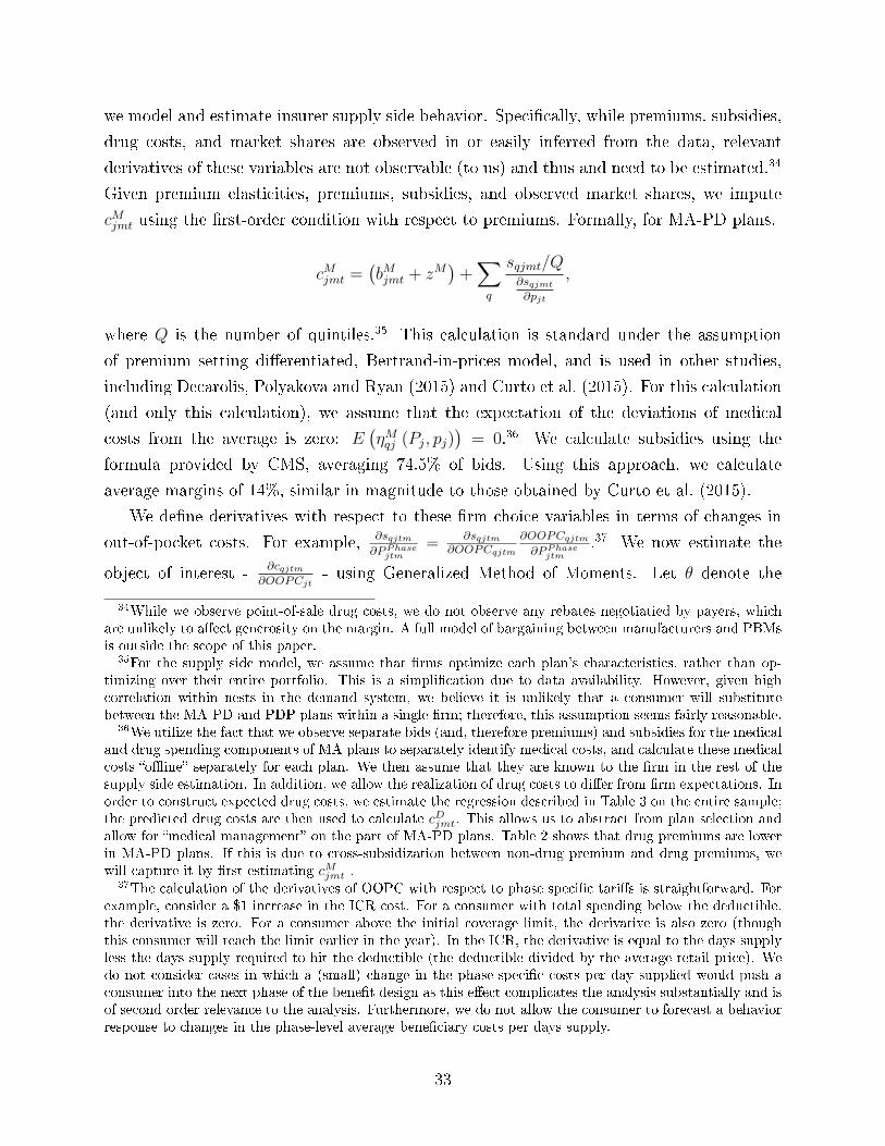
we model and estimate insurer supply side behavior. Speci�cally, while premiums, subsidies,

drug costs, and market shares are observed in or easily inferred from the data, relevant

derivatives of these variables are not observable (to us) and thus and need to be estimated.34

Given premium elasticities, premiums, subsidies, and observed market shares, we impute

cMjmt using the �rst-order condition with respect to premiums. Formally, for MA-PD plans,

cMjmt =(bMjmt + zM

)+∑q

sqjmt/Q∂sqjmt

∂pjt

,

where Q is the number of quintiles.35 This calculation is standard under the assumption

of premium setting di�erentiated, Bertrand-in-prices model, and is used in other studies,

including Decarolis, Polyakova and Ryan (2015) and Curto et al. (2015). For this calculation

(and only this calculation), we assume that the expectation of the deviations of medical

costs from the average is zero: E(ηMqj (Pj, pj)

)= 0.36 We calculate subsidies using the

formula provided by CMS, averaging 74.5% of bids. Using this approach, we calculate

average margins of 14%, similar in magnitude to those obtained by Curto et al. (2015).

We de�ne derivatives with respect to these �rm choice variables in terms of changes in

out-of-pocket costs. For example, ∂sqjtm∂PPhase

jtm

=∂sqjtm

∂OOPCqjtm

∂OOPCqjtm

∂PPhasejtm

.37 We now estimate the

object of interest -∂cqjtm

∂OOPCjt- using Generalized Method of Moments. Let θ denote the

34While we observe point-of-sale drug costs, we do not observe any rebates negotiatied by payers, whichare unlikely to a�ect generosity on the margin. A full model of bargaining between manufacturers and PBMsis outside the scope of this paper.

35For the supply side model, we assume that �rms optimize each plan's characteristics, rather than op-timizing over their entire portfolio. This is a simpli�cation due to data availability. However, given highcorrelation within nests in the demand system, we believe it is unlikely that a consumer will substitutebetween the MA-PD and PDP plans within a single �rm; therefore, this assumption seems fairly reasonable.

36We utilize the fact that we observe separate bids (and, therefore premiums) and subsidies for the medicaland drug spending components of MA plans to separately identify medical costs, and calculate these medicalcosts �o�ine� separately for each plan. We then assume that they are known to the �rm in the rest of thesupply side estimation. In addition, we allow the realization of drug costs to di�er from �rm expectations. Inorder to construct expected drug costs, we estimate the regression described in Table 3 on the entire sample;the predicted drug costs are then used to calculate cDjmt. This allows us to abstract from plan selection andallow for �medical management� on the part of MA-PD plans. Table 2 shows that drug premiums are lowerin MA-PD plans. If this is due to cross-subsidization between non-drug premium and drug premiums, wewill capture it by �rst estimating cMjmt .

37The calculation of the derivatives of OOPC with respect to phase speci�c tari�s is straightforward. Forexample, consider a $1 increase in the ICR cost. For a consumer with total spending below the deductible,the derivative is zero. For a consumer above the initial coverage limit, the derivative is also zero (thoughthis consumer will reach the limit earlier in the year). In the ICR, the derivative is equal to the days supplyless the days supply required to hit the deductible (the deductible divided by the average retail price). Wedo not consider cases in which a (small) change in the phase-speci�c costs per day supplied would push aconsumer into the next phase of the bene�t design as this e�ect complicates the analysis substantially and isof second order relevance to the analysis. Furthermore, we do not allow the consumer to forecast a behaviorresponse to changes in the phase-level average bene�ciary costs per days supply.

33

expectation of this derivative. The �rst-order conditions imply that:

∑q

[(pDjmt + zDt + 1(MA)

(bMjmt + zMmt

)−(cDqjmt + 1(MA)cMqjmt

)) ∂sqjmt

∂OOPCqjmt

∂OOPCqjmt

∂P Phasejmt

+

θ∂OOPCqjmt

∂P Phasejmt

sqjmt] = 0.

H(P, p) does not enter this formulation directly because the costs and subsidies are allowed

to vary by quintile directly. As premiums or generosity changes, the plan attracts a di�erent

mix of consumers (across quintiles), which accommodates the potential for selection.

There is a straightforward mapping from di�erent values of this parameter to levels of

drug spending by �rms. Intuitively, the more �expensive� it is to make plans more generous,

due to asymmetric information or the absence of o�sets, the less willing the �rm is to increase

generosity. Figure A.7 illustrates the basic logic of our identi�cation argument using average

values of the derivatives of shares with respect to premiums and out-of-pocket costs, and

Table 10 describes how all of the critical quantities are calculated or estimated.38

4.4.1 Supply Side Parameter Estimates

We parametrize θ using four di�erent speci�cations; in each, the constant term represents

the percentage of an out-of-pocket cost increase (reduction) that is passed on to the insurer

in the form of savings (costs). First, we simply estimate one parameter for all plans, noting

that without asymmetric information or o�sets, θ = −1. The presence of selection and o�sets

will both lead to estimates of θ that di�er from (negative) one. If more generous plans attract

sicker consumers, increasing out-of-pocket costs will attract healthier consumers, lowering

insurer costs more than one-for-one. If there are o�sets and drug demand slopes down,

higher out-of-pocket costs will increase non-drug medical costs. The estimates are in Table

8. The constant in the �rst speci�cation implies that a $100 increase in out-of-pocket costs

saves the average insurer $100 in drug (and, potentially, medical) costs. Among stand-alone

PDP plans, a $100 increase in out-of-pocket costs saves the average insurer $103, consistent

with selection (less generous plans attract di�erent types consumers), or moral hazard (less

generous plans have lower utilization).

In order to estimate the impact of o�sets directly, we isolate the portion of θ that is unique

to MA-PD plans by allowing θ to di�er across MA-PD and PDP plans: θ = θ1 +θ2×1(MA).

In this parameterization, we allow θ to vary with the type of plan; the impact of increasing

generosity in a MA-PD plan is simply the sum of the two coe�cients. The results show that

38On the x-axis, we plot di�erent values of the derivative of interest, denoted by θ, while on the y-axis,we plot insurer spending. The results are slightly di�erent across di�erent phases, but illustrate that thesmaller in absolute value θ is, the more the plan spends on drugs.

34

Table 8: Supply Results∂c/∂OOPC (1) (2) (3) (4)Constant -0.9973 -1.0323 -1.0323 -1.0323

(0.0098) (0.0109) (0.0109) (0.0109)MA 0.3488 0.2160 0.3521

(0.0341) (0.0474) (0.0673)MA*Normalized Non-Drug Costs 0.1383

(0.0230)MA*Normalized 3-year Retention Rate 0.0305

(0.0931)Plan-Market-Year Obs. 34,431 34,431 34,431 34,431

Notes: Parameters are estimated using generalized method of moments as describedin Section 4. Standard errors are calculated using a bootstrap that re-samples planswith replacement and presented in parentheses.

the relationship between plan generosity and insurer costs is statistically di�erent across

di�erent types of plans. The constant term indicates that the average stand-alone PDP

would save $91 per member by increasing out-of-pocket costs by $103, while the second term

indicates that the average MA-PD plan would only save $68 per member by increasing out-of-

pocket costs by $100. Because MA costs are given as cjmt = cDjmt+cMjmt, the derivative of MA-

PD costs with respect to phase speci�c prices can be written as∂cjmt

∂PPhasejmt

=∂cDjmt

∂PPhasejmt

+∂cMjmt

∂PPhasejmt

.39

Our results indicate that as MA-PD plans spend more on drugs, some of the insurer's cost

is o�set by reductions in spending in other areas.40

We explore heterogeneity in the size of the o�set e�ect along two dimensions. The size of

the o�set e�ect may depend on the illness severity of the consumers in the plan; the reduced

form results implied higher potential o�sets among consumers with chronic conditions. In

order to test this hypothesis, we interact the Medicare Advantage dummy with the implied

medical, non-drug spending in that plan (which avoids a mechanical relationship between

spending and the magnitude of the o�set term), normalized to have a mean of zero and

a standard deviation of one. The results are in the third column of Table 8 and imply a

bigger o�set among the sickest consumers. A MA-PD plan with average non-drug spending

two standard deviations larger than average would save only $54 by increasing out-of-pocket

costs by $100, due in part to a larger o�set of non-drug costs. In addition, the o�set e�ect

might vary with consumer tenure, as insurers will be more likely to invest in enrollee health

(that saves money over time) if enrollees stay in plans for extended periods. While the results

39We note that cjmt at the plan level is just the enrollment-weighted average over quintiles.40The di�erence between the spending implied in Figure A.7 is largely consistent with the reduced form

estimates for the entire sample.

35

in the �nal column are not statistically signi�cant, they are consistent with this hypothesis.

4.5 Robustness

In this section, we test the robustness of the model to assumptions along three dimensions.

First, we explore the extent to which selection in combination imperfect risk selection may

in�uence our results. We then examine the impact of regulatory constraints and, �nally, we

examine the impact of behavioral biases of consumers at the plan choice stage.

In order to address the role of selection in the determination of contract characteristics

more directly, we model plan choice as a function of contract characteristics.41 In these

speci�cations, we include premiums, OOPC, and dummies for deductible and donut hole

coverage as the observable characteristics. Following Decarolis, Polyakova and Ryan (2015),

we use plan vintage as a proxy for switching costs. Consistent with previous results, we �nd

evidence of selection with respect to donut hole coverage in Table 9: consumers with higher

2006 drug consumption (our measure of severity) have a higher preference for donut hole

coverage. In contrast, the results in Table 7 imply that sicker consumers are slightly less

sensitive to both premiums and OOPC. One concern is that this last result could be driven

by increased OOPC measurement error among sicker consumers and that could have broader

implications for our base estimates. In order to address this, we examine the sensitivity of our

supply side estimates to to di�erences in preferences over plan generosity of sicker consumers.

In unreported speci�cations, we �nd that increasing the plan generosity elasticity of sicker

consumers a�ects our mean estimate of θ1, but not the principle parameter of interest, the

interaction with the MA plan dummy (θ2).42

By allowing heterogeneity across severity types in preferences and unobserved plan quality

(through di�erent �xed e�ects for severity type), we can allow implied plan marginal costs

(net of risk adjustment) and the changes in these marginal costs to di�er across severity

classes. Because of the �exibility of our demand system, we believe our baseline approach

removes the confounding unobservables that would bias parameter estimates and thus we

accurately capture plan incentives for choosing plan characteristics in our setting.43

41This is in contrast to our current approach, which relies on plan �xed e�ects and identi�es sensitivity toprice and OOPC using cross market variation.

42This �nding is consistent with a greater degree of adverse selection but no di�erence in o�sets acrossseverity levels. These results are available from the authors upon request. Furthermore, as stated above,increased measurement error among sicker enrollees could drive this pattern in our preferred estimates.

43Table 11 shows that the results are similar if we use variation from only the ICR price, which eliminatesany concerns about selection with respect to donut hole coverage. The main estimate is now greater thanone in absolute value, consistent with adverse selection along this margin. However, the di�erential e�ectfor MA-PD plans (θ2) is quite similar to our main speci�cations. In unreported regressions, we also estimateour model with the two tari�s directly. While the results are qualitatively similar, we note that the tari�sare highly correlated, leading to noisier coe�cients. Finally, while di�erential reinsurance and risk corridorsmay have a small e�ect on our results, we believe their impact is directionally ambiguous (Medpac (2015b)).

36

In Section 4.2, we highlighted a number of regulatory features of this market that may

a�ect �rm incentives. In particular, distortions created by the LIS subsidy could a�ect our

main results. Insurers may alter product characteristics in response to the LIS program. De-

carolis, Polyakova and Ryan (2015) account for this possibility in their analysis. Following

their approach, we restrict attention to those contracts that bid above the LIS benchmark

amount in the majority of regions in which they operate and re-estimate the supply side pa-

rameters, assuming that these remaining contracts will not be distorted by the structure of

the LIS subsidy. This restriction leaves fewer contracts available to estimate the parameters.

Nevertheless, the results (presented in Table 11) are qualitatively similar to our main speci-

�cation indicating that our basic results hold even allowing for the LIS distortion. Similarly,

in the bottom panel of Table 11, we restrict attention to �enhanced� plans that are unlikely

to be constrained by minimum plan generosity requirements; the results are quantitatively

similar.44

Our reduced form results show that di�erences in plan generosity are most pronounced

among drugs believed a priori to have large o�sets. We can reconstruct our plan character-

istics to focus on cost sharing for this subset of drugs and re-estimate θ; in this exercise, we

are assuming that the level of coverage for these drugs alone is set optimally. The results

are in the second panel of Table 11; because di�erences among these drugs drive much of

the variation in plan characteristics by plan type, the results are qualitatively similar.

Finally, our demand model is in the neoclassical, static tradition and does not capture

the possibility that consumers may meaningfully deviate from that framework in selecting

plans. These deviations could a�ect both the measurement and the interpretation of our

results. Handel (2013) documents plan choice inertia in the employer-sponsored setting and

Ho, Hogan and Scott Morton (2015) document inertia in the Part D setting. To examine

the robustness of our results to our static demand assumption, we repeat our entire analysis

focusing on active choosers who are more likely to behave like neoclassical consumers. We

de�ne active choosers as consumers either aging into the Medicare program or switching

plans.45 Table 9 shows that these active consumers are more sensitive to both premiums

and OOPC, but the relative magnitudes of the coe�cients is consistent. We recompute our

supply side model using these demand estimates; Table 11 shows that the results are, again,

quite similar to the main speci�cation.46

44We de�ne a plan as �enhanced� if it has a supplemental premium in at least half of all markets in whichit operates. This accounts for 7% of all stand-alone plans. The analysis omitting LIS plans serves as anadditional robustness check along this dimension as plans not eligible for LIS enrollment are also likely tobe more generous than the minimum actuarial standard. These two subsets overlap substantially.

45This is, of course, is endogenous; this issue is addressed directly in Ho et al. (2015).46We can also estimate our results using a balanced panel of plans (those available since 2006). As shown

in Table 7, the results are again similar.

37

5 Counterfactuals

To quantify the importance of the o�set, we �rst consider how PDP plans would adjust

plan generosity if they were forced to account for non-drug medical costs in the same way

as their counterparts in the MA program. Mechanically, we set θPDP = θ̂MA and then

resolve for a new equilibrium. We allow drug costs to the insurer, cDrugjmt , to adjust to account

for the new incentives. We solve for drug costs, rather than phase-speci�c average out-of-

pocket costs, for two reasons. First, drug costs enter into the plan's �rst order condition

directly. Second, from a policy perspective, we are primarily interested in impact of di�erent

incentives on drug spending.47The �rst column of Table 9 presents the baseline results. The

average MA-PD plan has lower premiums (due to generous reimbursement) than the average

PDP plan, which have average premiums of $407 per year. By contrast, the average MA-

PD plan spends almost $75 dollars more per year on drugs ($1285 versus $1211) once we

account for selection, similar to our reduced form results. In the lower panel of Table 9, we

report the results of a simulation in which premiums are not allowed to adjust, but PDP

plans internalize the o�set. In this counterfactual, we see that the average PDP plan would

spend 11% more on prescription drugs if they took the entire medical o�set into account.

In addition, we note that MA-PD plans increase their spending as well � plan generosity

is a strategic complement, and there is no implicit trade o� between higher generosity and

higher premiums. Next we report the results of a counterfactual exercise in which insurers

are allowed to adjust both drug spending and premiums. Here, PDP plans increase their

spending by roughly the same amount, but also increase their premiums (15%) to o�set some

of the additional drug costs.

Our estimates quantify how changes in cost sharing arrangements a�ect insurers' cost

structure. By combining our estimates with estimates of the observed behavioral response

to cost sharing by consumers, we can calculate the implied o�sets and the impact of coun-

terfactual policies. We take estimates of the behavioral response to cost sharing from Einav,

Finkelstein and Schrimpf (2015), who estimate a dynamic model of drug consumption.48

Consider a small out-of-pocket cost decrease from P0 to P1. This price decrease will increase

insurer drug costs by an amount equal to the drug point-of-sale price less out-of-pocket cost

for the marginal units, plus the price di�erence times all of the infra-marginal units. We

know from the supply side estimation that the increase in insurer costs associated with low-

47Mechanically, costs change to �t the model in which the elasticity is taken as given and consumptionincreases as tari�s change.

48The elasticity is identi�ed by exploiting the kink in individuals' budget sets created by the donut hole;we reproduce their elasticity estimates in Table 12 and use the elasticity for a 1% uniform out-of-pocket costreduction of -0.54 in our calculation.

38

Table 9: CounterfactualsBaseline �Sophisticates�:

αp = αP

MA PDP MA PDPPremium 206.00 407.93 206.00 407.93% Change - - - -Insurer Rx Spend 1285.25 1211.62 1357.41 1337.64% Change - - 0.0564 0.1038

Internalize Externality: θPDP = θ̂MA

Premium 206.00 407.93 231.42 459.22% Change - - 0.0409 0.1498Insurer Rx Spend 1352.62 1347.72 1337.38 1394.30% Change 0.0528 0.1114 0.1182 0.1288PremiumAdjustment no yes

Notes: Results are calculated as described in Section 5. Means across markets arereported, as well as the % change from baseline. Drug spending represents theinsured costs.

ering OOPC to consumers is smaller for MA-PD plans than stand-alone PDP plans. This

implies there must be a shadow drug cost, c′ < c that applies to MA-PD plans. From the

observed behavioral elasticity we can infer the increase in quantity. Therefore, we can com-

pute the distance between c′ and c such that the magnitude of implied o�sets rationalizes

�rm behavior; the magnitude of this di�erence is equal to ∂cMedical

∂P.49

For a 1% uniform decrease in cost sharing, denoted by P, we calculate the implied

di�erence in insurer costs for MA-PD plans as (omitting subscripts for simplicity):

∂cMedical

∂P= θ2

∂OOPC

∂P,

which gives the di�erence in the change in insurer costs between MA-PD plans and stand-

alone PDP plans. The shadow drug costs is simply the point-of-sale cost less implied o�sets.

This quantity must be equal to the change in quantity times the di�erence in the drug cost

and the shadow drug cost:∂q

∂P(c− c′).

We use the value of θ2 (0.35) estimated in Table 8 and the mechanical value of ∂OOPC∂P

,

49Does c′ represent the drug cost less the total savings in medical expenditure? No; the shadow drug costonly takes insurer medical costs cMedical

jmt into account and is therefore strictly higher than the �true� shadowcost. This has important implications for welfare, as discussed in Glazer and McGuire (2013).

39

$10.15.50 We take ∂q∂P

directly from Einav, Finkelstein and Schrimpf (2015), and use the

average empirical value of c ($2.20). Solving for c′, we get $1.78. Put di�erently, the

�discount� implied by o�sets is 49 cents per day supplied, or 22%.

The o�set we calculate is very close to previous estimates and obtained using supply side

variation. Our counterfactuals show that stand-alone PDP plans would spend $135 more per

year, implying an o�set of $23.18 per enrollee per year. Multiplying this by 17.5 million, the

number of stand-alone PDP enrollees in 2008, we �nd that PDP plans impose an externality

of $520 million per year; based on our bootstrapped estimates, the 99% con�dence interval

for this estimate ranges from $466 million per year to $583 million per year.51 By contrast,

McWilliams et al. (2016) �nd that the much-discussed Medicare Shared Savings Program led

to an aggregate $238 million spending reduction in the early years; our larger results indicate

the potential power of incentive alignment in equilibrium. Our results illustrate the value of

insurer incentive alignment in the Medicare Advantage program and the potential of more

e�cient bene�t design by private insurers, who may align bene�t design more e�ciently than

the federal government (see also Finkelstein, Einav and Polyakova (2016)).52

Furthermore, Table 12 shows that it would be costly for the government to achieve

increased drug consumption generated by MA-PD plans using a �at cost sharing subsidy

alone; this calculation highlights the advantage of nimbler private insurers. However, there

is no reason that the pro�t maximization incentives of MA-PD plans necessarily align with

any social welfare criterion. Therefore, another natural policy intervention would be to

better align consumer plan choices with value (from a societal perspective, including any

externalities on the traditional Medicare program). To see why such a policy could improve

market outcomes, note that our estimates imply two potential sources of behavioral biases.

First, higher spending in MA-PD plans is consistent with underutilization; the insurer has an

incentive to address this friction and appears to do so, at least in part, by reducing the out-of-

pocket drug costs to its enrollees. Second, consumers appear to undervalue reductions in out-

of-pocket costs at the plan choice stage.53 This behavior has two consequences. Consumers

50For this calculation, we use the average value of consumer out-of-pocket cost per day supplied and theformula described in Section 4.2, evaluated at average consumption.

51We would obtain a similar estimate if we used the implied additional spending by PDP plans in Table9. By contrast, MedPAC (Medpac (2015a)) estimates that spending on an equivalent enrollee in a MA-PDplans is approximately 2% higher than traditional Medicare. The average total Medicare spending wasapproximately $10,000 per enrollee in 2008 (an $200 of additional spending in MA); the externality due too�sets does not, on its own, imply greater e�ciency in MA-PD plans. However, the externality providesevidence of a potential channel through which MA-PD plans can obtain e�ciency gains.

52 To give additional context, the changes in MA overpayments due to risk adjustment policies measured in

Brown et al. (2014) are approximately $317, or about twice as large as our causal increase in drug spending.

53This is clear because a $1 reduction in OOPC is valued at less than a $1 reduction in premiums by

40

enroll in �sub-optimal� plans in the sense that they would be in better �nancial and physical

health (via increased the drug consumption) if they placed more weight on the expected

out-of-pocket costs of the plan. In addition, and perhaps more importantly, there would be

a supply response by insurers if enrollees placed more weight on the expected out-of-pocket

costs. We quantify the size of this supply response.

In our �nal counterfactual, we consider the impact of better aligning consumer preferences

with neoclassical views on optimal decision making. One way to align consumer decision

utility with value is to provide targeted consumer search tools that better highlight the

trade-o�s between plan premiums and generosity (Handel and Kolstad (2015)). In this

setting, we believe that would lead consumers to place greater weight on out-of-pocket costs

(Ericson and Starc (2013)) and lead to reduced naivete about potential under-consumption.

Mechanically, we implement this by setting the coe�cient on OOPC in the demand system

equal to the coe�cient on premiums, such that consumers treat a $1 increase in premiums

equal to a $1 increase in OOPC. The results are in the �nal two columns of the top panel of

Table 9. If consumers were "sophisticated," plans would increase their generosity. MA-PD

plans would spend 5.6% more on prescription drugs, while PDP plans would spend 10.4%

more. This increased spending by standalone PDP plans is less than the amount that fully

internalizes the �scal externality, yet shows that public policies that align consumer demand

or the structure of subsidies with providing value will incentivize insurers to o�er contracts

that reduce costs or increase health.

6 Conclusion

This paper examines how health insurers react to both over-utilization and, particularly,

underutilization by consumers. We build on empirical literatures that estimate structural

models of insurer decisions and model endogenous product characteristics to show how cost-

side incentives a�ect insurance design. We examine these issues in the Medicare Advantage

and Part D markets and show that di�erences in incentives across plan types drive the

generosity of the bene�ts.

We �nd causal evidence that MA-PD plans spend more on drugs than their stand-alone

counterparts; this increased spending is concentrated in those drug categories with large

o�sets and among consumers with chronic conditions. Our model of �rm behavior highlights

the mechanisms that drive this di�erential: MA-PD plans have an incentive to internalize

the e�ect of drug o�sets. By measuring �rm incentives, we are able to calculate the size

of the implied o�set. Our estimate of an approximately 20% o�set is similar in magnitude

to demand-side estimates. This implies that �rms take o�sets into account when designing

consumers.

41

plans and may be able to mitigate ine�cient underutilization by consumers. Finally, the

counterfactuals show how policy changes can increase plan incentives to help consumers

internalize o�sets.

These results highlight the importance of the intersection of consumer choice in health

care markets and contract design by �rms in oligopolistic settings. Our work shows that

incentives meaningfully a�ect plan design features, which in turn impact both health and

health care costs. This work also highlights the important role that government policy plays

in determining how market forces will work in the private provision of Medicare bene�ts.

42

References

Abaluck, J. and J. Gruber. 2011. �Choice Inconsistencies among the Elderly: Evidence from

Plan Choice in the Medicare Part D Program.� American Economic Review 101(4):1180�

1210.

Abaluck, Jason, Jonathan Gruber and Ashley Swanson. 2015. �Prescription Drug Use under

Medicare Part D: A Linear Model of Nonlinear Budget Sets.� NBER Working Paper No.

20976.

Afendulis, C. C., Yulei He, Alan M. Zaslavsky and M. E. Chernew. 2011. �The Impact of

Medicare Part D on Hospitalization Rates.� Health Services Research 46(4):1022�1038.

Afendulis, Christopher C, Michael E Chernew and Daniel P Kessler. 2013. �The E�ect of

Medicare Advantage on Hospital Admissions and Mortality.� NBER Working Paper No.

19101.

Baicker, K., M. E. Chernew and J. Robbins. 2013. �The Spillover E�ect of Medicare Man-

aged Care: Medicare Advantage and Hospital Utilization.� Journal of Health Economics

32:1289�1300.

Baicker, Katherine, Sendhil Mullainathan and Joshua Schwartzstein. 2015. �Behavioral Haz-

ard in Health Insurance.� Quarterly Journal of Economics 130(4):1623�1667.

Berry, St. 1994. �Estimating Discrete Choice Models of Product Di�erentiation.� RAND

Journal of Economics 25:242�262.

Brot-Goldberg, Zarek C, Amitabh Chandra, Benjamin R Handel and Jonathan T Kolstad.

2015. �Consumer Heterogeneity and Medical Care Price Responsiveness: Evidence and

Implications for Optimal Insurance Design.� NBER Working Paper No. 21632.

Brown, J.., M. Duggan, I. Kuziemko and W. Woolston. 2014. �How Does Risk-Selection Re-

spond to Risk-Adjustment: Evidence from the Medicare Advantage Program.� American

Economic Review 104(10).

Cabral, M., M. Geruso and N. Mahoney. 2014. �Does Privatized Health Insurance Bene�t

Patients or Producers? Evidence from Medicare Advantage.� NBER Working Paper No.

20470.

Carey, C.M. 2015. �Technological Change and Risk Adjustment: Bene�t Design Incentives

in Medicare Part D.� Cornell University.

43

CBO. 2012. O�setting E�ects of Prescription Drug Use on Medicares Spending for Other

Health Care Services. Technical report Congressional Budget O�ce.

Chandra, Amitabh, Jonathan Gruber and Robin McKnight. 2010. �Patient cost-sharing and

hospitalization o�sets in the elderly.� American Economic Review 100(1):193.

Chernew, Michael E, Allison B Rosen and A Mark Fendrick. 2007. �Value-based insurance

design.� Health A�airs 26(2):w195�w203.

Crawford, G. 2012. �Accommodating Endogenous Product Choices: A Progress Report.�

International Journal of Industrial Organization 30:315�320.

Curto, V., L. Einav, J. Levin and J. Bhattacharya. 2015. �Can Health Insurance Competition

Work? Evidence from Medicare Advantage.� NBER Working Paper No. 20818.

Dalton, Christina M., Gautam Gowrisankaran and Robert Town. 2015. �Myopia and Com-

plex Dynamic Incentives: Evidence from Medicare Part D.� NBER Working Paper No.

21104.

Decarolis, F. 2015. �Medicare Part D: Are Insurers Gaming the Low Income Subsidy Design?�

American Economic Review 105(4):1547�80.

Decarolis, Francesco, Maria Polyakova and Steven P. Ryan. 2015. �The Welfare E�ects of

Supply-Side Regulations in Medicare Part D.� NBER Working Paper No. 21298.

Draganska, M., M. Mazzeo and K. Seim. 2009. �Beyond plain vanilla: Modeling joint product

assortment and pricing decisions.� Quantative Marketing and Economics 7(2).

Duggan, Mark, Amanda Starc and Boris Vabson. 2015. �Who Bene�ts when Government

Pays more? Pass-through in the Medicare Advantage Program.� NBER Working Paper

No. 19989.

Duggan, Mark and Fiona Scott Morton. 2010. �The Impact of Medicare Part D on Pharma-

ceutical Prices and Utilization.� American Economic Review 100(1):590�607.

Einav, Liran, Amy Finkelstein and Paul Schrimpf. 2015. �The response of drug expenditures

to non-linear contract design: Evidence from Medicare Part D.� Quarterly Journal of

Economics 130(2):841�899.

Eizenberg, A. 2014. �Upstream Innovation and Product Variety in the U.S. Home PC Mar-

ket.� Review of Economic Studies 81:1003�1045.

44

Ellis, Randall P., Shenyi Jiang andW. Manning. 2015. �Optimal health insurance for multiple

goods and time periods.� Journal of Health Economics 41:89�106.

Ellison, Glenn. 2006. Bounded rationality in industrial organization. Vol. 42 Cambridge

University Press p. 142.

Ericson, K.M. and A. Starc. 2013. �How Product Standardization A�ects Choice: Evidence

from the Massachusetts Health Insurance Exchange.� NBER Working Paper No. 19527.

Fan, Y. 2013. �Ownership Consolidation and Product Characteristics: A Study of the US

Daily Newspaper Market.� American Economic Review 103(5):1598�1628.

Fang, Hanming and Alessandro Gavazza. 2011. �Dynamic Ine�ciencies in an Employment-

Based Health Insurance System: Theory and Evidence.� American Economic Review

101:3047�3077.

Finkelstein, A., L. Einav and M. Polyakova. 2016. �Private Provision of Social Insurance:

Drug-speci�c Price Elasticities and Cost Sharing in Medicare Part D.� NBER Working

Paper No. 22277.

Finkelstein, A., M. Gentzkow and H. Williams. 2016. �Sources of Geographic Variation in

Health Care: Evidence from Patient Migration.� NBER Working Paper 20789.

Gaynor, M., J. Li and W. Vogt. 2007. �Substitution, Spending O�sets, and Prescription

Drug Bene�t Design.� Forum for Health Economics and Policy 10(2):1�31.

Glazer, J. and T. McGuire. 2013. �A Welfare Measure of O�set E�ects in Health Insurance.�

Journal of Public Economics 96(5-6):520�523.

Goldman, D. and Tomas J. Philipson. 2007. �Integrated Insurance Design in the Presence

of Multiple Medical Technologies.� American Economic Review 97(2):427�432.

Gowrisankaran, G., K. Norberg, S. Kymes, M. E. Chernew, D. Stwalley, L. Kemper and W.

Peck. 2013. �A Hospital System's Wellness Program Linked To Health Plan Enrollment

Cut Hospitalizations But Not Overall Costs.� Health A�airs .

Grubb, Michael D. 2012. �Dynamic nonlinear pricing: Biased expectations, inattention, and

bill shock.� International Journal of Industrial Organization 30(3):287�290.

Grubb, Michael D. 2014. �Consumer inattention and bill-shock regulation.� The Review of

Economic Studies 82(1):219�257.

45

Grubb, Michael D and Matthew Osborne. 2012. �Cellular service demand: Biased beliefs,

learning, and bill shock.� American Economic Review 105(1):234�271.

Handel, B. R. 2013. �Adverse Selection and Inertia in Health Insurance Markets: When

Nudging Hurts.� American Economic Review 103(7):2643�2682.

Handel, B. R. and J. T. Kolstad. 2015. �Getting the Most From Marketplaces: Smart Policies

on Health Insurance Choice.� Brookings Hamilton Project Discussion Paper 2015-08.

Ho, K., J. Hogan and F. Scott Morton. 2015. �The Impact of Consumer Inattention on

Insurer Pricing in the Medicare Part D Program.� NBER Working Paper No. 21028.

Hoadley, J., L. Summer, E. Hargrave, J. Cubanski and T. Neuman. 2014. �Medicare Part D

in Its Ninth Year: The 2014 Marketplace and Key Trends, 2006-2014.�.

Ketcham, J., C. Lucarelli, E. Miravete and M. Roebuck. 2012. �Sinking, Swimming, or

Learning to Swim in Medicare Part D.� American Economic Review 102(6):2639�2673.

Lavetti, K. and K. Simon. 2014. �Strategic Formulary Design in Stand-Alone and Integrated

Medicare Advantage Prescription Drug Plans.�.

Lustig, J. 2010. �Measuring welfare losses from adverse selection and imperfect competition

in privatized medicare.� Boston University Department of Economics.

Manning, W., J. Newhouse, N. Duan, E. Keeler, B. Benjamin, A. Leibowitz and M. Marquis.

1987. �Health Insurance and the Demand for Medical Care: Evidence from a Randomized

Experiment.� American Economic Review 77(3):251�277.

McGuire, T., J. Newhouse and A. Sinaiko. 2011. �An Economic History of Medicare Part

C.� The Milbank Quarterly .

McWilliams, J. Michael, Alan M. Zaslavsky and Haiden A. Huskamp. 2011. �Implementation

of Medicare Part D and Nondrug Medical Spending for Elderly Adults With Limited Prior

Drug Coverage.� The Journal of the American Medical Association 306(4):402�409.

McWilliams, J.M., L. Hat�eld, M.E. Chernew, B. Landon and A. Schwartz. 2016. �Early

Performance of Accountable Care Organizations in Medicare.� New England Journal of

Medicine 374:2357�2366.

Medpac. 2015a. �The Medicare Advantage program: Status report.�.

Medpac. 2015b. Report to the Congress: Medicare and the Health Care Delivery System.

Technical report Medpac.

46

NICE. 2011. Hypertension in adults: diagnosis and management. Technical report National

Institute for Health and Care Excellence.

Nosal, K. 2011. �Estimating Switching Costs for Medicare Advantage Plans.� Mannheim.

Stockley, K., T. McGuire, C. C. Afendulis and M. E. Chernew. 2014. �Premium Transparency

in the Medicare Advantage Market: Implications for Premiums, Bene�ts, and E�ciency.�

NBER Working Paper No. 20208.

Sweeting, A. 2010. �The E�ects of Mergers on Product Positioning: Evidence from the Music

Radio Industry.� RAND Journal of Economics 41(2):372�97.

Wollman, T. 2016. �Trucks without bailouts: Equilibrium product characteristics for com-

mercial vehicles.�.

47

A Drug Classi�cation (For Online Publication)

We follow Chandra, Gruber and McKnight (2010) in classifying drugs in three categories.

Category 1 drugs are �acute care drugs are those that, if not taken, will increase the probabil-

ity of an adverse health event within a month or two.� These drugs comprise approximately

40% of total drug spending. Category 2 contains �chronic care medications are designed

to treat more persistent conditions that, if not treated, will result in a potentially adverse

health event within the year (examples include analgesics, antivirals, ACE inhibitors, ' med-

ications, beta-blockers, hypertension drugs, statins, and glaucoma medications).� Category

3 are �medications that, while necessary to improve patients' quality of life, will not result

in an adverse health event if not taken, because they provide symptom relief as opposed

to a�ecting the underlying disease process (examples are acne medications, antihistamines,

motion sickness medications, cold remedies, relief of pain drugs).�

The classes included in Category 1 are Adrenal Corticosteroids, Aminoglycosides, Ana-

phylaxis Treatment Kits, Anesthesia, Anthelmintics, Antianginals, Antiarrhythmics, An-

tiasthmatics/broncodilators, Antibacterials, Miscellaneous, Antibiotics, Alkaloids, And En-

zymes, Anticoagulants/thrombolytics, Anticonvulsants, Antidotes, Antimalarials, Antimetabo-

lites, Antimycobacterials, Antineoplastics, Antiprotozoals, Antipsychotics/antimanics, Anti-

toxins/antivenins, Blood Components/substitutes, Blood Glucose Regulators, Cardiac Gly-

cosides, Cardiovascular-renal, Cephalosporins, Chloramphenicol/derivatives, Coronary Va-

sodilators, Dna Damaging Drugs, Hypotension/shock, Lincosamides and macrolides, Ocular

Anti-infective/anti-in�ammator, Penicillins, Polymyxins, Quinolones/derivatives, Repl/regs

Of Electrolytes/water Balance, Respiratory Tract, Sulfonamides/related Compounds, Tetra-

cyclines, Vascular Disorders, and Cerebral/peripheral. We exclude drugs that are believed

to have di�erential selection e�ects, as described in Lavetti and Simon (2014). Drug lists

for each category were compiled using lists from drugs.com. Respiratory tract drugs include

drugs used to treat asthma and COPD. For drugs with multiple uses, the drug was only

included under its primary usage (e.g. etanercept is sometimes used to treat Alzheimer's

Disease, but is much more commonly used for autoimmune diseases such as rheumatoid

arthritis, psoriatic arthritis, plaque psoriasis and ankylosing spondylitis. Thus, it is not

included on the list of Alzheimer's drugs).

We also note that additional drugs have been introduced since the time period stud-

ied in Chandra, Gruber and McKnight (2010) and that clinical guidelines evolve over time.

Therefore, we also consider an alternative, more recent set of classes targeted by a value

based insurance design program implemented by Blue Cross Blue Shield of North Carolina

(BCBSNC) in addition to other examples from the commercial market (Chernew, Rosen and

48

Fendrick (2007); Gowrisankaran et al. (2013)). These plans target chronic conditions includ-

ing asthma, diabetes, hypertension, and hyperlipidemia. Sample restrictions are described

in the notes for Figures 5 and A.1.

49

B Additional Robustness Checks (For Online Publica-

tion)

Figure A.1: Price E�ects by Drug Class

Notes: This �gure plots the di�erences in prices by plan type. Other hypertensiondrugs include ACE inhibitors, angiotensin II receptor antagonists, renin inhibitors,antiadrenergic agents (centrally & peripherally acting), alpha-adrenergic blockers,aldosterone receptor antagonists, vasodilators and antihypertensive combinationtherapies. Standard errors are clustered at the plan-product level.

Figure A.2: E�ect of Population on MA Plan Rebates

Notes: Plots a binscatter with �fty population bins using data from 2008 using datafrom Medicare Landscape Files. We drop counties with FFS costs above the urban�oor. Lines represent a linear �t.

50

Figure A.3: E�ect of Population on Sample Demographics

Notes: Plots a binscatter with �fty population bins using 2008 data. We dropcounties with FFS costs above the urban �oor, and control for bene�ciary age, sex,race, 2006 spending type, and county-level FFS costs. Lines represent a quadratic�t.

Figure A.4: E�ect of Population on Sample Demographics

Notes: Plots a binscatter with �fty population bins using 2008 data. We dropcounties with FFS costs above the urban �oor, and control for bene�ciary age, sex,race, 2006 spending type, and county-level FFS costs. Lines represent a quadratic�t.

Figure A.5: E�ect of Population on Sample Demographics

Notes: Plots a binscatter with �fty population bins using 2008 data. We dropcounties with FFS costs above the urban �oor, and control for bene�ciary age, sex,race, 2006 spending type, and county-level FFS costs. Lines represent a quadratic�t.

51

Figure A.6: E�ect of Population on FFS Spending

Notes: Plots a binscatter with �fty population bins using the �ve year movingaverage from 2004, when �oors were formally (but not practically) discontinued. Wedrop counties with FFS costs above the urban �oor. Lines represent a quadratic �t.

Figure A.7: Supply Side Identi�cation

Notes: This �gure plots the optimal level of insurer spending under alternativelevels of θ from �rst-order conditions from both P ICR and PDonut, using averagevalues of the derivatives of shares with respect to premiums and out-of-pocket costs.

52

Table A.1: T-test ResultsMetro Population <250K >250K t-test valuePrimary Care Physicians/Resident (2010) 0.000553 0.000575 -0.666

(0.000336) (0.000330)Total MDs/Resident (2005) 0.00172 0.00163 0.474

(0.00198) (0.00148)Inpatient Service Unit Beds/Resident (2012) 0.00107 0.000941 1.307

(0.00103) (0.000952)Inpatient Days Per Resident (2005) 0.745 0.690 0.565

(0.974) (0.928)Medicare Enrollment Per Resident (2005) 0.127 0.127 0.1947

(0.00181) (0.00240)Percentage of Population Male (2005) 0.493 0.494 -0.458

(0.0322) (0.0280)Number of Observations 289 148

Median Age (2010) 38.124 38.941 -1.689*(5.126) (4.171)

Race (2010):White 81.986 81.351 0.419African American 9.739 11.527 -1.312

(13.047) (14.607)American Indian/Alaskan 1.220 0.872 0.930

(4.325) (2.143)Asian 1.449 1.445 0.0162

(2.560) (1.436)Hispanic/Latino 8.401 6.703 1.409

(12.972) (9.870)Number of Observations 296 150

MA Plan Rebate 61.28 64.11 -2.83MA Premium 25.97 23.43 2.55Out-of-Pocket Medical Costs 400.21 392.59 7.63**Number of Observations 292 150

Notes: Table A.1 presents t-test results comparing counties with fewer than 250,000residents to those with greater than 250,000 residents using data from the AreaHealth Resources File 2014-2015 release. When available, statistics from 2005 areused, otherwise the closest available year to 2005 is used. Race is measured aspercentage. Standard deviations are in parentheses. Median age is signi�cant at the10% level.

53

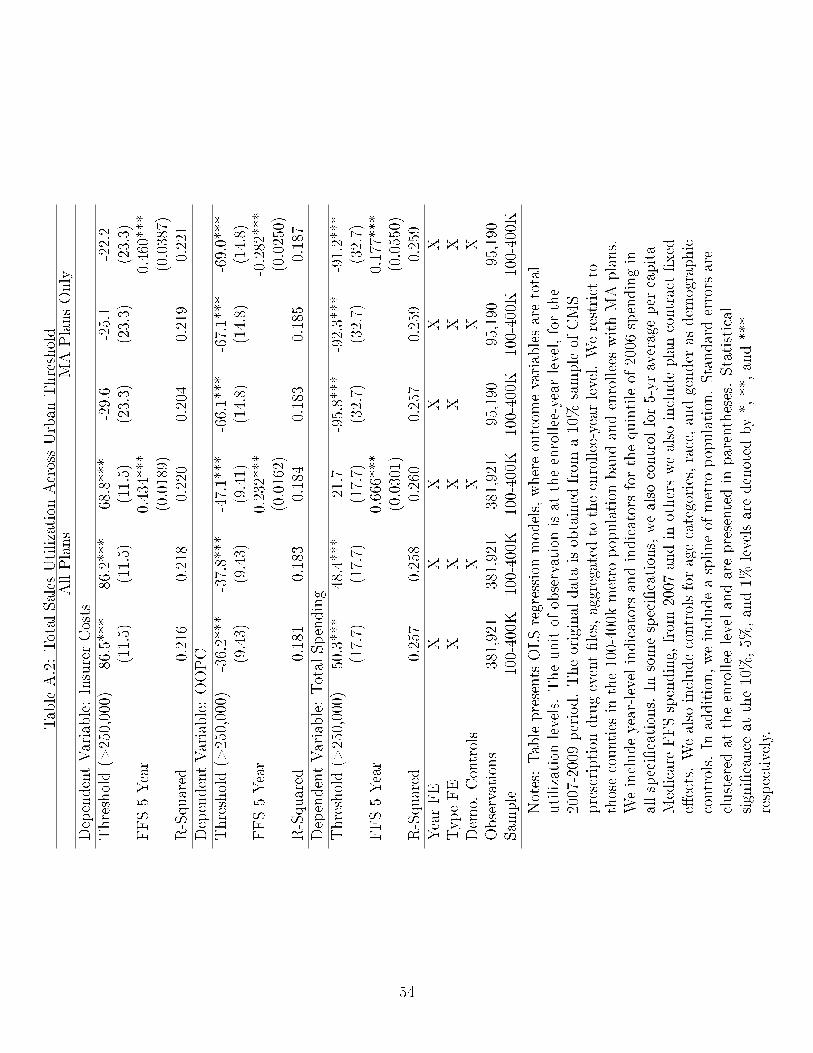
TableA.2:TotalSales

Utilization

AcrossUrban

Threshold

AllPlans

MAPlansOnly

DependentVariable:InsurerCosts

Threshold(>

250,000)

86.5***

86.2***

68.8***

-29.6

-25.1

-22.2

(11.5)

(11.5)

(11.5)

(23.3)

(23.3)

(23.3)

FFS5Year

0.434***

0.460***

(0.0189)

(0.0387)

R-Squared

0.216

0.218

0.220

0.204

0.219

0.221

DependentVariable:OOPC

Threshold(>

250,000)

-36.2***

-37.8***

-47.1***

-66.1***

-67.1***

-69.0***

(9.43)

(9.43)

(9.41)

(14.8)

(14.8)

(14.8)

FFS5Year

0.232***

-0.282***

(0.0162)

(0.0250)

R-Squared

0.181

0.183

0.184

0.183

0.185

0.187

DependentVariable:TotalSpending

Threshold(>

250,000)

50.3***

48.4***

21.7

-95.8***

-92.3***

-91.2***

(17.7)

(17.7)

(17.7)

(32.7)

(32.7)

(32.7)

FFS5Year

0.666***

0.177***

(0.0301)

(0.0550)

R-Squared

0.257

0.258

0.260

0.257

0.259

0.259

YearFE

XX

XX

XX

TypeFE

XX

XX

XX

Dem

o.Controls

XX

XX

Observations

381,921

381,921

381,921

95,190

95,190

95,190

Sam

ple

100-400K

100-400K

100-400K

100-400K

100-400K

100-400K

Notes:Tablepresents

OLSregression

models,whereoutcom

evariablesaretotal

utilization

levels.Theunitof

observationisat

theenrollee-yearlevel,forthe

2007-2009period.Theoriginaldataisobtained

from

a10%

sampleof

CMS

prescription

drugevent�les,aggregated

totheenrollee-yearlevel.Werestrict

tothosecounties

inthe100-400k

metro

population

bandandenrolleeswithMAplans.

Weincludeyear-levelindicatorsandindicatorsforthequintileof

2006

spendingin

allspeci�cations.

Insomespeci�cations,wealso

controlfor5-yraverageper

capita

MedicareFFSspending,from

2007

andin

otherswealso

includeplancontract�xed

e�ects.Wealso

includecontrolsforagecategories,race,andgender

asdem

ographic

controls.

Inaddition,weincludeasplineof

metro

population.Standarderrors

are

clustered

attheenrollee

levelandarepresentedin

parentheses.Statistical

signi�cance

atthe10%,5%

,and1%

levelsaredenoted

by*,**,and***

respectively.

54

Table A.3: Mechanisms - Medicare Protected Class Products Only(1) (2)

Outcome: Logged OOPC/Day1(MA) -0.117*** -0.0974

(0.0073) (0.0076)Constant -0.925*** -2.132***

(0.0044) (0.0131)Observations 9,568,940 9,568,940Adjusted R-Squared 0.580 0.679Product Fixed E�ects X XPhase Fixed E�ects XAll Products X XProtected Classes Only X X

Notes: Table presents linear regression models, where outcome variables are asdescribed in each panel. This table only includes drugs that are considered�Protected Classes� by Medicare. This includes anti-cancer, ant-psychotic,anti-convulsant, anti-depressant, immuno-suppresant and HIV/AIDS drugs. Theunit of observation is at the �ll level, for the 2007-2009 period. The original data isobtained from a 10% sample of CMS prescription drug event �les. We includeyear-level indicators and product �xed e�ects in all speci�cations. In somespeci�cations, we also control the phase of the standard Part D bene�t. Standarderrors are clustered at the product level and are presented in parentheses. Statisticalsigni�cance at the 10%, 5%, and 1% levels are denoted by *, **, and ***respectively.

55

TableA.4:RobustnessChecks

DependentVariable:InsurerCosts

1(MA)

615.7***

610.4***

402.6***

514.2***

506.7***

387.5***

535.0***

481.2***

376.5***

(89.99)

(90.69)

(76.60)

(74.25)

(73.34)

(68.38)

(75.45)

(74.03)

(69.62)

FFS5Year

0.681***

0.506***

0.413***

(0.0512)

(0.0226)

(0.0221)

Mean

0.093

0.096

0.163

0.114

0.119

0.159

0.058

0.083

0.114

DependentVariable:OOPC

1(MA)

152.4**

157.5**

27.41

-215.2***

-222.2***

-265.2***

-249.1***

-288.6***

-304.4***

(66.92)

(67.48)

(57.49)

(55.51)

(54.92)

(52.74)

(55.01)

(54.81)

(52.73)

FFS5Year

0.426***

0.183***

0.0626***

(0.0425)

(0.0183)

(0.0174)

R-Squared

0.142

0.144

0.172

0.193

0.194

0.192

0.154

0.154

0.153

DependentVariable:TotalSpending

1(MA)

768.1***

767.9***

430.0***

299.0***

284.6***

122.3

285.8**

192.6*

72.08

(135.0)

(136.3)

(113.4)

(108.0)

(106.7)

(100.7)

(112.0)

(110.3)

(105.1)

FFS5Year

1.107***

0.688***

0.476***

(0.0803)

(0.0343)

(0.0344)

R-Squared

0.155

0.156

0.219

0.230

0.233

0.252

0.168

0.183

0.193

YearFE

XX

XX

XX

XX

XTypeFE

XX

XX

XX

XX

XDem

o.Controls

XX

XX

XX

Observations

91,270

91,270

91,270

381,921

381,921

381,921

424,436

424,436

424,436

Sam

ple

200-300K

200-300K

200-300K

100-400K

100-400K

100-400K

100-400K

100-400K

100-400K

Low

FFSCounties

Includes

zero

utilization

bene�ciaries

Notes:Tablepresents

instrumentalvariableregression

models,whereoutcom

evariablesareinsurerandbene�ciarycostsandtotalutilization

levels.Theunitof

observationisat

theenrollee-yearlevel,forthe2007-2009period.Theoriginaldata

isobtained

from

a10%

sampleof

CMSprescription

drugevent�les,aggregated

totheenrollee-yearlevel.Werestrict

tothosecounties

described

inthesamplerow.

Weincludeyear-levelindicatorsandindicatorsforthequintileof

2006

spendingin

allspeci�cations.

Wealso

controlfor5-yraverageper

capitaMedicareFFS

spendingfrom

2007.Wealso

includecontrolsforagecategories,race,andgender

asdem

ographiccontrols.

Inaddition,weincludeasplineof

metro

population.

Standarderrors

areclustered

attheenrollee

levelandarepresentedin

parentheses.

Statisticalsigni�cance

atthe10%,5%

,and1%

levelsaredenoted

by*,**,and***

respectively.

56

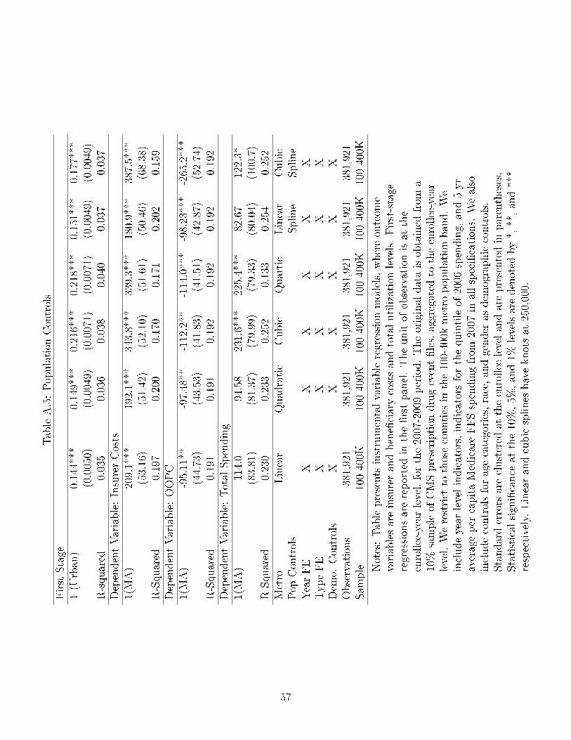
TableA.5:Population

Controls

First

Stage

1(U

rban)

0.144***

0.149***

0.216***

0.218***

0.151***

0.177***

(0.0050)

(0.0049)

(0.0071)

(0.0071)

(0.0049)

(0.0049)

R-squared

0.035

0.036

0.038

0.040

0.037

0.037

DependentVariable:InsurerCosts

1(MA)

209.1***

192.1***

343.8***

339.3***

180.9***

387.5***

(53.16)

(51.42)

(52.10)

(51.61)

(50.46)

(68.38)

R-Squared

0.197

0.200

0.170

0.171

0.202

0.159

DependentVariable:OOPC

1(MA)

-95.11**

-97.48**

-112.2**

-114.0***

-98.23***

-265.2***

(44.73)

(43.53)

(41.83)

(41.51)

(42.87)

(52.74)

R-Squared

0.191

0.191

0.192

0.192

0.192

0.192

DependentVariable:TotalSpending

1(MA)

114.0

94.58

231.6***

225.4***

82.67

122.3*

(83.81)

(81.37)

(79.99)

(79.33)

(80.04)

(100.7)

R-Squared

0.230

0.233

0.252

0.133

0.254

0.252

Metro

Linear

Quadratic

Cubic

Quartic

Linear

Cubic

Pop

Controls

Spline

Spline

YearFE

XX

XX

XX

TypeFE

XX

XX

XX

Dem

o.Controls

XX

XX

XX

Observations

381,921

381,921

381,921

381,921

381,921

381,921

Sam

ple

100-400K

100-400K

100-400K

100-400K

100-400K

100-400K

Notes:Tablepresents

instrumentalvariableregression

models,whereoutcom

evariablesareinsurerandbene�ciarycostsandtotalutilization

levels.First-stage

regressionsarereportedin

the�rstpanel.Theunitof

observationisat

the

enrollee-yearlevel,forthe2007-2009period.Theoriginaldataisobtained

from

a10%

sampleof

CMSprescription

drugevent�les,aggregated

totheenrollee-year

level.Werestrict

tothosecounties

inthe100-400k

metro

population

band.We

includeyear-levelindicators,indicatorsforthequintileof

2006

spending,and5-yr

averageper

capitaMedicareFFSspendingfrom

2007

inallspeci�cations.

Wealso

includecontrolsforagecategories,race,andgender

asdem

ographiccontrols.

Standarderrors

areclustered

attheenrollee

levelandarepresentedin

parentheses.

Statisticalsigni�cance

atthe10%,5%

,and1%

levelsaredenoted

by*,**,and***

respectively.Linearandcubicsplines

haveknotsat

250,000.

57

Table A.6: Impact of MA Enrollment on Spending, Non-LIS Distorted(1) (2) (3) (4) (5) (6)

OLS IVDependent Variable: Insurer Drug Costs1(MA) -76.44*** -78.73*** -75.80*** 502.0*** 495.9*** 376.5**

(3.973) (3.978) (3.977) (74.05) (73.16) (68.20)FFS 5 Year 0.433*** 0.507***Avg. Spend (0.0189) (0.0226)R-Squared 0.217 0.219 0.221 0.116 0.121 0.161Dependent Variable: OOPC1(MA) -181.3*** -178.5*** -177.1*** -220.2*** -225.9*** -270.1***

(2.855) (2.865) (2.868) (55.37) (54.77) (52.59)FFS 5 Year 0.203*** 0.187***Avg. Spend (0.0160) (0.0184)R-Squared 0.194 0.196 0.196 0.194 0.195 0.193Dependent Variable: Total Drug Spending1(MA) -257.7*** -257.3*** -252.9*** 281.1*** 270.0** 106.5

(6.857) (5.878) (5.880) (107.7) (106.4) (100.3)FFS 5 Year 0.544*** 0.694***Avg. Spend (0.0328) (0.0344)R-Squared 0.264 0.265 0.267 0.232 0.234 0.253Year FE X X X X X XType FE X X X X X XDemo. X X X XControlsN 377,391 377,391 377,391 377,391 377,391 377,391Sample 100-400K 100-400K 100-400K 100-400K 100-400K 100-400K

Notes: Table presents linear regression models, where outcome variables are insurerand bene�ciary costs and total utilization levels. The unit of observation is at theenrollee-year level, for the 2007-2009 period. The original data is obtained from a10% sample of CMS prescription drug event �les, aggregated to the enrollee-yearlevel. We restrict to those counties in the 100-400k metro population band and toplans with less than 50% low-income subsidy enrollees nationally. We includeyear-level indicators and indicators for the quintile of 2006 spending in allspeci�cations. In some speci�cations, we also control for 5-yr average per capitaMedicare FFS spending, from 2007. We also include controls for age, age squared,race, and gender as demographic controls. In addition, we include a spline of metropopulation. Standard errors are clustered at the enrollee level and are presented inparentheses. Statistical signi�cance at the 10%, 5%, and 1% levels are denoted by *,**, and *** respectively.

58

Table A.7: Impact of MA Enrollment on Spending Including Patients over Catastrophic Cap(1) (2) (3) (4) (5) (6)

OLS IVFirst Stage, Dependent Variable: MA Enrollment1 (Urban) 0.163*** 0.165*** 0.173***

(0.00767) (0.00767) (0.00768)FFS 5 Year XR-squared 0.026 0.036 0.037Dependent Variable: Insurer Drug Costs1(MA) -83.20*** -89.30*** -84.85*** 1,294*** 1,277*** 1,067***

(12.20) (12.19) (12.18) (283.0) (279.8) (269.0)FFS 5 Year 0.656*** 0.842***Avg. Spending (0.0541) (0.0643)R-Squared 0.068 0.069 0.070 . . 0.017Dependent Variable: OOPC1(MA) -232.4*** -228.8*** -227.2*** -204.9*** -217.8*** -275.2***

(3.851) (3.865) (3.869) (79.02) (78.07) (74.72)FFS 5 Year 0.238*** 0.231***Avg. Spending (0.0218) (0.0252)R-Squared 0.199 0.200 0.200 0.199 0.200 0.200Dependent Variable: Total Drug Spending1(MA) -315.6*** -318.1*** -312.0*** 1,090*** 1,059*** 792.2***

(14.13) (14.13) (14.13) (314.9) (311.2) (298.4)FFS 5 Year 0.894*** 1.073***Avg. Spending (0.0670) (0.0784)R-Squared 0.127 0.127 0.128 0.077 0.080 0.098Year FE X X X X X XType FE X X X X X XDemo. Controls X X X XObservations 398988 398988 398988 398988 398988 398988Sample 100-400K 100-400K 100-400K 100-400K 100-400K 100-400K

Notes: Table presents linear regression models, where outcome variables are insurerand bene�ciary costs and total utilization levels. The unit of observation is at theenrollee-year level, for the 2007-2009 period. The original data is obtained from a10% sample of CMS prescription drug event �les, aggregated to the enrollee-yearlevel. We restrict to those counties in the 100-400k metro population band. Weinclude year-level indicators and indicators for the quintile of 2006 spending in allspeci�cations. In some speci�cations, we also control for 5-yr average per capitaMedicare FFS spending, from 2007. We also include controls for age, age squared,race, and gender as demographic controls. In addition, we include a spline of metropopulation. Standard errors are clustered at the enrollee level and are presented inparentheses. Statistical signi�cance at the 10%, 5%, and 1% levels are denoted by *,**, and *** respectively.

59

Table 8: Impact of MA Enrollment on Spending, Including Patients not Enrolled in 2006(1) (2) (3) (4) (5) (6)

OLS IVFirst Stage, Dependent Variable: MA Enrollment1 (Urban) 0.142*** 0.145*** 0.150***

(0.00640) (0.00639) (0.00639)FFS 5 Year XR-squared 0.025 0.035 0.036Dependent Variable: Insurer Drug Costs1(MA) -99.05*** -95.01*** -92.28*** 243.7*** 211.1*** 95.39

(3.573) (3.589) (3.593) (78.67) (76.89) (73.31)FFS 5 Year 0.430*** 0.457***Avg. Spending (0.0184) (0.0213)Observations 557,819 557,819 556,514 557,819 557,819 556,514R-Squared 0.004 0.011 0.013 0.003First Stage, Dependent Variable: MA Enrollment1 (Urban) 0.0849*** 0.0884*** 0.0873***

(0.00780) (0.00778) (0.00777)FFS 5 Year XR-squared 0.114 0.114 0.114Dependent Variable: Insurer Drug Costs1(MA) -59.90*** -59.14*** -58.98*** 531.8*** 407.0*** 431.8***

(3.975) (3.978) (3.978) (157.7) (147.8) (150.2)FFS 5 Year 0.112*** 0.153***Avg. Spending (0.0304) (0.0340)R-Squared 0.169 0.175 0.175 0.077 0.119 0.112Year Fixed E�ects X X X X X XType Fixed E�ects X X X X X XDemographic Controls X X X XObservations 424,436 424,436 424,436 424,436 424,436 424,436Sample 100-400K 100-400K 100-400K 100-400K 100-400K 100-400K

Notes: Table presents linear regression models, where outcome variables are insurerand bene�ciary costs and total utilization levels. The unit of observation is at theenrollee-year level, for the 2007-2009 period. The original data is obtained from a10% sample of CMS prescription drug event �les, aggregated to the enrollee-yearlevel. We restrict to those counties in the 100-400k metro population band. Weinclude year-level indicators in all speci�cations. In some speci�cations, we alsocontrol for 5-yr average per capita Medicare FFS spending, from 2007. We alsoinclude controls for age, age squared, race, and gender as demographic controls. Inaddition, we include a spline of metro population. Indicators for the quintile of 2006spending are not included as they are not available for all enrollees. Standard errorsare clustered at the enrollee level.

60

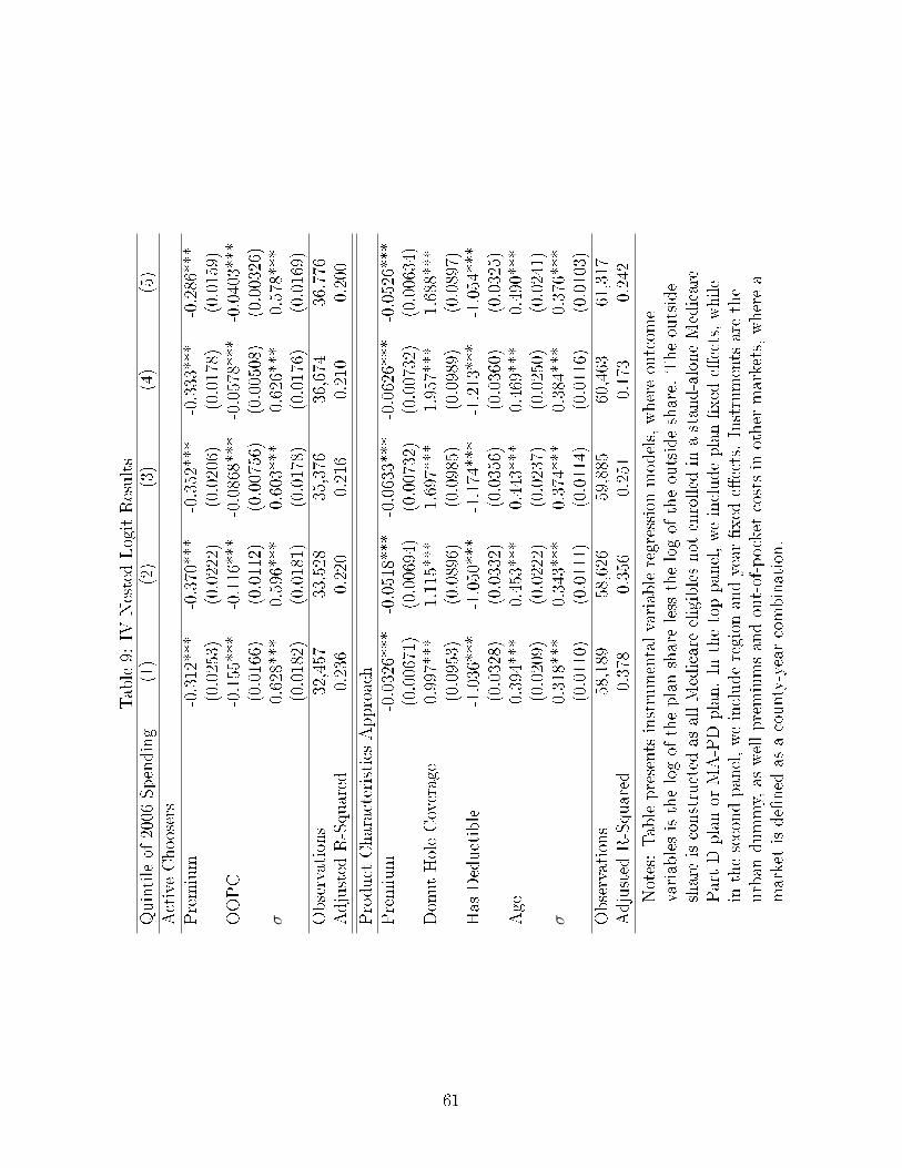
Table9:

IVNestedLogitResults

Quintileof

2006

Spending

(1)

(2)

(3)

(4)

(5)

ActiveChoosers

Premium

-0.312***

-0.370***

-0.352***

-0.333***

-0.286***

(0.0253)

(0.0222)

(0.0206)

(0.0178)

(0.0159)

OOPC

-0.155***

-0.116***

-0.0868***

-0.0578***

-0.0403***

(0.0166)

(0.0112)

(0.00756)

(0.00508)

(0.00326)

σ0.628***

0.596***

0.603***

0.626***

0.578***

(0.0182)

(0.0181)

(0.0178)

(0.0176)

(0.0169)

Observations

32,457

33,528

35,376

36,674

36,776

Adjusted

R-Squared

0.236

0.220

0.216

0.210

0.200

Product

CharacteristicsApproach

Premium

-0.0326***

-0.0518***

-0.0633***

-0.0626***

-0.0526***

(0.00671)

(0.00694)

(0.00732)

(0.00732)

(0.00634)

DonutHoleCoverage

0.997***

1.115***

1.697***

1.957***

1.688***

(0.0953)

(0.0896)

(0.0985)

(0.0989)

(0.0897)

Has

Deductible

-1.036***

-1.050***

-1.174***

-1.213***

-1.054***

(0.0328)

(0.0332)

(0.0356)

(0.0360)

(0.0325)

Age

0.394***

0.453***

0.443***

0.469***

0.490***

(0.0209)

(0.0222)

(0.0237)

(0.0250)

(0.0241)

σ0.318***

0.343***

0.374***

0.384***

0.376***

(0.0110)

(0.0111)

(0.0114)

(0.0116)

(0.0103)

Observations

58,189

58,626

59,885

60,463

61,317

Adjusted

R-Squared

0.378

0.356

0.251

0.173

0.242

Notes:Tablepresents

instrumentalvariableregression

models,whereoutcom

evariablesisthelogof

theplanshareless

thelogof

theoutsideshare.

Theoutside

shareisconstructed

asallMedicareeligiblesnot

enrolled

inastand-aloneMedicare

PartDplanor

MA-PDplan.In

thetoppanel,weincludeplan�xed

e�ects,while

inthesecondpanel,weincluderegion

andyear

�xed

e�ects.Instruments

arethe

urban

dummy,as

wellpremiumsandout-of-pocket

costsin

other

markets,wherea

marketisde�ned

asacounty-yearcombination.

61

Table 10: Identi�cationObject Inferencepjtm data, observed separately for drug and medical componentsrPDPqt , rMA

qmt datacMjmt inferred from pricing decision using �Part C� bids and subsidies,

MA plans onlycDqjmt data, expectation formed using speci�cation in Table 3∂sqjmt

∂pjtmcalculated from demand estimates

∂sqjmt

∂PPhasejt

calculated from demand estimates

∂cDrugqjmt

∂PPhasejt

mechanical function of phase-speci�c out-of-pocket costs

sqjmt data∂cMqjmt

∂PPhasejt

object of interest

Table 11: Supply Results∂c/∂OOPC (1) (2) (3) (4) (5) (6)

Non-LIS Distorted Active Choosers ICR Price OnlyConstant -1.0530 -1.0897 -1.1156 -1.1714 -1.0530 -1.0897

(0.0120) (0.0117) (0.0510) (0.0002) (0.0120) (0.0117)MA 0.3613 0.5568 0.3613

(0.0330) (0.1040) (0.0330)Plan-Market-Year Obs. 33,884 33,884 34,431 34,431 34,431 34,431

(7) (8) (9) (10) (11) (12)Basic Plans Alt. Rebate Lg. O�set Drugs

Price OnlyConstant -0.9604 -0.9604 -0.9984 -1.0323 -0.9986 -1.0323

(0.0104) (0.0104) (0.0085) (0.0093) (0.0087) (0.0092)MA 0.4802 0.3375 0.3355

(0.0055) (0.0320) (0.0303)Plan-Market-Year Obs. 33,906 33,906 34,431 34,431 34,431 34,431

Notes: Parameters are estimated using generalized method of moments as describedin Section 4. Standard errors are calculated using a bootstrap that re-samples planswith replacement.

62

Table12:CounterfactualPolicies

Uniform

Elasticity

O�set

Change

inOOPC

E�ective

Cost

%Change,

Consumer

Valuation,

OOPCReduction

(toGovernment)

PDPPenetration

OOPCReduction(U

B)

1.00%

-0.54

3.54

10.15

6.61

-0.0010

4.30

2.50%

-0.38

6.23

25.28

19.06

-0.0030

10.70

5.00%

-0.33

10.82

50.51

39.69

-0.0064

21.38

10.00%

-0.30

19.67

100.94

81.28

-0.0132

42.74

25.00%

-0.29

47.53

252.30

204.77

-0.0342

106.82

50.00%

-0.29

95.06

504.60

409.54

-0.0744

213.64

75.00%

-0.31

152.43

757.27

604.84

-0.1224

320.61

EliminatetheDonutHole

52.4

355.99

303.58

-0.0571

152.86

Notes:Resultsarecalculatedas

described

inSection

5.

63

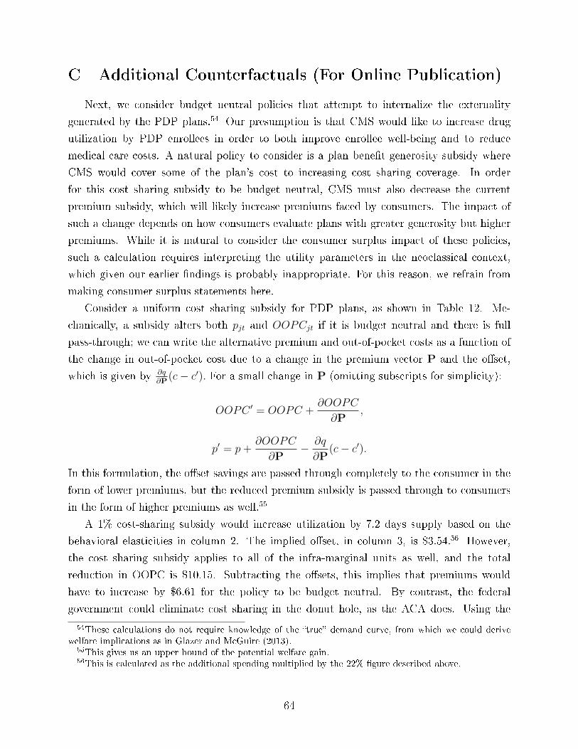
C Additional Counterfactuals (For Online Publication)

Next, we consider budget neutral policies that attempt to internalize the externality

generated by the PDP plans.54 Our presumption is that CMS would like to increase drug

utilization by PDP enrollees in order to both improve enrollee well-being and to reduce

medical care costs. A natural policy to consider is a plan bene�t generosity subsidy where

CMS would cover some of the plan's cost to increasing cost sharing coverage. In order

for this cost sharing subsidy to be budget neutral, CMS must also decrease the current

premium subsidy, which will likely increase premiums faced by consumers. The impact of

such a change depends on how consumers evaluate plans with greater generosity but higher

premiums. While it is natural to consider the consumer surplus impact of these policies,

such a calculation requires interpreting the utility parameters in the neoclassical context,

which given our earlier �ndings is probably inappropriate. For this reason, we refrain from

making consumer surplus statements here.

Consider a uniform cost sharing subsidy for PDP plans, as shown in Table 12. Me-

chanically, a subsidy alters both pjt and OOPCjt if it is budget neutral and there is full

pass-through; we can write the alternative premium and out-of-pocket costs as a function of

the change in out-of-pocket cost due to a change in the premium vector P and the o�set,

which is given by ∂q∂P

(c− c′). For a small change in P (omitting subscripts for simplicity):

OOPC ′ = OOPC +∂OOPC

∂P,

p′ = p+∂OOPC

∂P− ∂q

∂P(c− c′).

In this formulation, the o�set savings are passed through completely to the consumer in the

form of lower premiums, but the reduced premium subsidy is passed through to consumers

in the form of higher premiums as well.55

A 1% cost-sharing subsidy would increase utilization by 7.2 days supply based on the

behavioral elasticities in column 2. The implied o�set, in column 3, is $3.54.56 However,

the cost sharing subsidy applies to all of the infra-marginal units as well, and the total

reduction in OOPC is $10.15. Subtracting the o�sets, this implies that premiums would

have to increase by $6.61 for the policy to be budget neutral. By contrast, the federal

government could eliminate cost sharing in the donut hole, as the ACA does. Using the

54These calculations do not require knowledge of the �true� demand curve, from which we could derivewelfare implications as in Glazer and McGuire (2013).

55This gives us an upper bound of the potential welfare gain.56This is calculated as the additional spending multiplied by the 22% �gure described above.

64

calculations in Einav, Finkelstein and Schrimpf (2015), this would increase drug consumption

by 8%, generating o�sets amounting to $52.54 per consumer. However, this policy is also

expensive: while it reduces OOPC by $356 per consumer, this reduction comes at a cost net

of o�sets of $303. Therefore, if the policy is to be budget neutral, premiums will have to rise

dramatically.57

Furthermore, these policies reduce the market share of PDP plans. Consumers do not

value the increased generosity at its full cost, as re�ected in the measured decision utility;

they prefer plans with lower premiums and higher cost sharing. Therefore, we conclude that it

will be di�cult for the government to implement broad based changes to the Part D program

aimed at reducing externalities that are budget neutral.58 This is for two reasons: consumers

are not sophisticated with respect to potential underutilization and most implementable

policies fail to target marginal consumption e�ectively leading to expensive out-of-pocket

cost reductions on infra-marginal units. These results are consistent with a model in which

private insurers can better target and subsidize underutilized, high-value care. For example,

while the cost-sharing subsidy we describe is uniform, applying to all drugs, private MA-PD

insurers can implement more sophisticated contracts that better target increased utilization.

We see evidence of this in our reduced form results; Figure 5 shows that MA-PD plans have

lower out-of-pocket costs for exactly those drugs likely to generate the largest o�sets. While

they increase the complexity of insurance contracts and may exacerbate plan choice frictions,

targeted subsidies are more likely to be cost-e�ective. Therefore, it may be more reasonable

to encourage MA-PD enrollment; based on our estimates in Table 7, we believe this can be

done in a cost-e�ective way. For example, rather than closing the donut hole, the federal

government could increase MA benchmarks by $312 per year, plus the $23 in implied o�sets.

This would increase MA-PD market share by 7.4%.

57Exacerbating this is the fact that MA-PD plans become more generous in equilibrium, decreasing OOPCto consumers by $97 per year. We note that the ACA policy is not budget neutral.

58This includes the recent Part D Enhanced Medication Therapy Management (MTM) Model, whichincentivizes stand-alone plans to reduce Parts A and B spending among their bene�ciaries. The actual�nancial incentives associated with this program are quite small. If plans reduce Parts A and B spendingby 2% (about $200 in 2008), they are eligible for a $2 per member per month increase in their benchmarkpayment. Because �rms only receive approximately one-tenth of the savings, they are unlikely to be in-centivized to internalize the externality created by prescription drug o�sets. Furthermore, we note that aPDP plan that fully internalized the externality would only spend an addition $153 per bene�ciary per year.Given our calculations, this would lead to savings in Parts A and B of about $30. We �nd that a policythat provides a $12.75 per member per month increase in the benchmark payment (and reduces Parts A andB spending by 0.3%) internalizes the externality, and would increase MA-PD enrollment by 3.4 percentagepoints. Furthermore, we note that a $153 increase is likely to represent the �rms' entire pro�t margins,based on a 15% pro�t margin and the estimates in Ho, Hogan and Scott Morton (2015).

65