EXTERNALITIES AND PRICING ON MULTIDIMENSIONAL

MATCHING PLATFORMS∗

Melati Nungsari†

Davidson College

Sam Flanders‡

UNC-Chapel Hill

Job Market Paper

October 7, 2015

Abstract

We study multidimensional matching on a two-sided platform operated by a profit-maximizing monop-olist. Utility is assumed to be non-transferable. Agents on one side of the market have preferencesover both homogeneous and heterogenous dimensions. Homogenous traits can be interpreted as verticalcharacteristics, where all agents agree on the ranking of the characteristic. In contrast, agents have dif-ferent preferences over heterogeneous traits. We find two previously unstudied externalities that resultfrom our matching framework. We call the first the rivalry externality and the second the no-transfersexternality. In particular, from a social welfare-maximizing perspective, we find that in a model withmultidimensional matching, agents tend to match too aggressively on traits that are homogeneous andnot aggressive enough on the heterogeneous dimensions. We show that these externalities are not uniqueto search models, but also appear in frictionless markets, such as those studied by Gale and Shapley[1962]. These two externalities have interesting pricing implications for the monopolist, who may find itoptimal to charge distortionary per-interaction prices to correct for them.

JEL classification: D21, C78, D83

Keywords: Externalities, Pricing, Monopolist, Matching, Search, Two-Sided Platforms

∗We would like to thank Gary Biglaiser, Peter Norman, Fei Li, Andy Yates, Helen Tauchen, and Sergio Parreiras at theEconomics Department at the University of North Carolina at Chapel Hill for their invaluable mentoring and help on thisresearch project. We would also like to thank the participants of the UNC Micro Theory Workshop for their comments thathave helped shaped this paper. Melati would also like to thank the Department of Economics at Davidson College for theirsupport. Last but not least, we both would like to thank the Royster Society of Fellows and the Economics Department atUNC-Chapel Hill for generously funding our years working on this project in graduate school. All mistakes are our own.†menungsari@davidson.edu; Economics Department at Davidson College, Box 7123, Davidson, NC 28035; 704-894-3123

(office phone); 309-299-1279 (cellphone); 704-894-3063 (fax).‡sflander@live.unc.edu; Economics Department at the University of North Carolina at Chapel Hill, 107 Gardner Hall, CB

#3305, Chapel Hill, NC 27599; 919-966-2383 (phone); 919-636-9852 (cellphone); 919-966-4986 (fax).

1

1 Introduction

This paper studies a two-sided matching platform operated by a profit-maximizing monopolist where agents

are searching for long-term partners and have preferences over multiple dimensions. When two individuals

decide to get married, each individual receives a matching utility and the partnership that forms results in

a matching surplus. There are two types of utility specifications that have been studied in the literature,

the first being transferable and the second, non-transferable. In transferable utility models, agents have the

ability to negotiate over the match surplus. In non-transferable utility models, such as the one presented in

our paper, agents do not have this ability. The allocation of match surplus to each individual is fixed, and

in particular, agents cannot pay others to marry them.

The literature on search and matching theory has primarily focused on cases where agents only care about

one characteristic when choosing whether or not to form a partnership. In reality, however, individuals

may have preferences over multiple characteristics in their potential match. For example, in assessing

whether or not you would like to marry a person you are dating, you may care simultaneously about their

physical attractiveness, income, weight, height, educational attainment, etc. In this paper, we study the

externalities that result from a multidimensional matching framework with non-transferable utility. We find

novel externalities that are endemic to multidimensional matching problems with non-transferable utility

and show, by embedding the matching model into a search and pricing framework, how a profit-maximizing

monopolist pursues surprising pricing strategies in response to these externalities.

In our model, agents have preferences over homogenous (or vertical) and heterogeneous characteristics.

Vertical or homogenous characteristics are traits for which agents agree on the ranking of the trait. For

example, income may be interpreted as a homogenous trait: everybody would prefer to match with a

richer individual. Preferences are more heterogenous to the extent that preference orderings vary among

individuals. In this stylized model, we will study an extreme case of heterogenous preferences where all

agents have preferences orderings that are uncorrelated. An example of a heterogenous characteristics is

race. Research has shown that most individuals in the U.S. do not marry partners from a different race.1

One common type of heterogeneous preferences is horizontal preferences, a la Hotelling [1929] and Salop

[1979]. For example, geographical location is a heterogenous characteristic. Agents may prefer partners

closer to them, and which potential matches are closer to them depends on their own locations.

1In fact, according to a Pew Research Center analysis on census data published in June 2015, only about 12% of marriagesin this country were between spouses of different races.

2

Two common externalities have been studied in matching markets: the thick-market externality and the

congestion externality. The thick-market externality results from the fact that agents do not internalize that

when they leave the market, they make it harder for other agents who may want to match with an agent

of their type to meet them. The congestion externality results from the fact that agents do not internalize

that by being on the platform, they may make it difficult for other agents to find a desirable match. This is

due to the fact that agents think that there are too many undesirable agents on the market to filter through

before getting to agents they would actually consider.

As mentioned before, our paper presents two previously unstudied matching externalities. We call the first

the rivalry externality and the second, the no-transfers externality. The rivalry externality is an externality

that exists due to the fact that agents make tradeoffs between all of the different dimensions of characteristics

that they match on. In particular, our main finding is that agents will match too aggressively on homogenous

traits versus heterogenous traits. This result is intuitive but not trivial: in pursuing their self-interests when

matching, the fact that all agents agree on the ranking of the homogenous traits causes a strong rivalry

effect—that is, if I am able to obtain the best potential match on the homogenous dimension, this means

that I am removing that person from the market and thus preventing other agents from meeting that person.

With more heterogeneous preferences, by contrast, my ideal match is less likely to be someone else’s ideal

match, so the rivalry effect is weaker. For example, if all agents’ preferences are uncorrelated, pursuing my

ideal match will not, in expectation, adversely affect the pool of potential matches for other matches.

The no-transfers externality exists due to the fact that utility is non-transferable and so agents are not

able to resolve any externalities privately by bargaining. We argue that the assumption of non-transferable

utility is reasonable for two important reasons. The first is that in dating, there may be social norms that

discourage an individual from paying another to marry them. The second is that there are clearly many

situations in which bargaining is quite costly—for example: high transaction costs, diminishing returns to

transfers, and credible commitment issues. These reasons may lead to an inability or distaste for bargaining.

In our model, the incentives of agents on the platform and the social welfare planner are not aligned. In

particular, agents only care about how good their own match is, while the social planner (i.e. the monopolist

firm operating the two-sided platform) cares about the total resulting match surplus. To see this, suppose that

there are two agents on each side of the market. Each agent is either a high type (stud) or a low type (dud).

Assuming that agents obtain their partner’s type when a match forms, note that the monopolist is indifferent

between two stud-dud partnerships forming and a stud-dud and a dud-dud partnership. Partnerships of the

3

first, however, might not form since the studs may not want to marry duds, who are inferior.

The rivalry and no-transfers externalities are not unique to search models. In particular, even though the

set up of our model is dynamic, our results focus on steady-state analysis, where the total inflows and total

outflows are equalized, leaving the distribution and mass of agents on the platform constant. Thus, although

we are focusing on an environment with search, we can also expect these externalities to appear in frictionless

models with non-transferable utility. We provide simulations to demonstrate this fact.

In order to study these externalities, we focus on the simplest model that can accommodate these mul-

tidimensional issues; that is, we will focus on the case where agents match on one homogenous and one

heterogenous dimension. Later in the paper, we will show how the results can be extended when matching

is on multiple dimensions. We will also check the robustness of the rivalry and no-transfers externalities

by performing simulations that relax some of the assumptions that we have made on the environment. We

present two simulations, both for markets with no search frictions and prices (i.e. the static matching model

presented by Gale and Shapley [1962]). The first simulation relaxes the assumption of modular utility that

we use in our model, where agents’ utility functions do not depend on their own type, to the more general

supermodular utility specification, where agents’ utilities exhibit increasing differences in their own types.

In our model, when agent’s match, they obtain a matching utility that is equal to the sum of their partner’s

vertical trait and an idiosyncratic matching shock, which is the same (perfectly correlated) for both agents.

The second simulation relaxes this assumption of perfectly correlated matching shocks.

Given these interesting externalities that result from our model, we then pose the question: how would a

profit-maximizing monopolist operating the platform price its services? We assume that the monopolist

utilizes a more general pricing structure (two-part tariff), where agents must pay a fixed fee to join the

platform, and then pay a per-interaction price for each draw of a new date while on the platform. We also

assume that types are perfectly observable, and so, the monopolist’s optimization problem is the same as

that of a social welfare maximizing entity. This is true since the monopolist’s objective is to maximize total

surplus generated on the platform, only to fully extract it using a combination of fixed and per-interaction

prices. This being, the monopolist will want to correct any externalities and deviations from the social

optimum. It does so in our model by using the only (imperfect) instrument available to them, which is the

per-interaction price.

As we shall see in the paper, in the model with no externalities (i.e. only one vertical type and the same

idiosyncratic matching shock for both sides), the optimal per-interaction price for the monopolist is zero. We

4

call this zero level of per-interaction prices as non-distortionary since they do not change the optimization

problem of the agent. In a model with observable types, the monopolist will charge a menu of per-interaction

prices for each type, i.e. p = (pH , pL) with corresponding fixed prices f = (fH , fL), which can be determined

from agent’s optimization problem. We will derive surprising pricing results in our paper—in particular,

depending on the parameterizations of the model, the monopolist may want to charge distortionary (i.e.

positive or negative) per-interaction prices to manipulate agents’ costs of staying and searching on the

platform. The fact that pL is positive is unsurprising—one may think of the low types as being inferior and

so, having more of them on the platform worsens the utility of everyone else, and in particular the high

types, who the monopolist cares about since they have more potential surplus to be extracted. One would

expect, however, that pH is set at the non-distortionary level. However, this is not the case since we find

cases where monopolist optimally charges a negative and positive pH .

The outline of the paper proceeds as follows. Section 2 first reviews the literature. Section 3 provides the

model setup. Section 4 studies the rivalry and no-transfers externalities and provides two simulations that

relax some of the assumptions made in the model. Section 5 studies the consequences of the externalities on

pricing, and Section 6 concludes.

2 Literature Review

This paper combines three literatures: search, matching, and pricing, The matching literature can be traced

back to the seminal paper by Gale and Shapley [1962]. Applications of matching theory to real-life markets

have included the kidney exchange market (Roth, Sonmez, and Unver [2005], Roth, Sonmez, and Unver

[2007], students to public school matching (Abdulkadiroglu, Pathak, and Roth [2005], Abdulkadiroglu et al.

[2005]), and the job search literature (Bulow and Levin [2006]). In terms of utility specifications, the first

two applications focus on non-transferable utility, which is similar to our paper. Bulow and Levin [2006],

however, model transferable utility, where wages are taken as prices. Aside from the utility specification,

another issue of interest when studying matching models is assortation. Positive assortation in equilibrium

implies that high types match with other correspondingly high types, whereas negative assortation means

that high types match with low types. Assuming non-transferable utility, Becker [1973] proved conditions

under which positive assortation occurs. As in many other matching papers, we also assume that matching

is random, exogenous, and non-targeted.

5

Previous papers in the literature have focused on matching where agents have preferences over only one

dimension. For example, in Burdett and Coles [1997], agents are vertically-differentiated with characteristics

summarized into a single number, defined as agent’s pizazz, which takes a value in the interval [0, 1]. Burdett

and Coles analyze the matching equilibrium by studying steady-state conditions and find a rich set of

equilibria. Agents match in assortative partitions in equilibrium, where the interval [0, 1] for both types of

agents is broken up into distinct pieces with agents in the same piece matching randomly with each other.

The search literature, on the other hand, started with the study of job search in the labor market (McCall

[1970], Burdett [1978], Mortensen and Pissarides [1994], Rogerson, Shimer, and Wright [2005]). It has since

expanded to include other applications as well, including the marriage and dating market (e.g. Cornelius

[2003]). Applications of search theory to the dating market usually assumes non-transferable utility, as this

mirrors real-life more closely than the assumption of transferable utility. In particular, Burdett and Wright

[1998] and Adachi [2003] both study properties of equilibria in a search models with non-transferable utility.

This paper incorporates pricing theory in a world with externalities and a profit-maximizing monopolist. We

study two cases: the first is when the monopolist can only operate one platform (perhaps due to high fixed

or operating costs), and the second is when monopolist has the ability to operate two platforms that cater

to the different types. This is in contrast to Rocher and Tirole [2010], who study platform competition with

two-sided markets. Pricing in search markets has also been studied by other authors (e.g. Bester [1994])

in the context of a buyer-seller relationship where buyers are looking to buy a good from a price-posting

seller. However, models such as Bester [1994] do not have the complexity of externalities which affect agent’s

optimal matching behavior in equilibrium, as in our model.

The closest paper related to the pricing framework in this paper Bloch and Ryder [2000], where they study

the provision of matching services in a model of two-sided search. Agents are distributed on the unit interval

and their utility is equal to the index of their mate. Bloch and Ryder [2000] find that in a search equilibrium,

agents form subintervals and are only matches to agents inside their own class, a result that closely mirrors

that of Burdett and Coles [1997]. The two main differences between our paper and theirs is my inclusion of

the heterogenous trait ψ and the fact that we assume that the monopolist utilizes a two-part tariff pricing

structure. We are primarily interested in the signs of the per-interaction prices–be it positive, the non-

distortionary (or, as we see later, the ‘no externalities’) level of 0, or even negative. Bloch and Ryder [2000],

on the other hand, study how two separate pricing structures (uniform and commissions on the matching

surplus) affect equilibrium behavior in agents. Another similar paper is Damiano and Li [2007], where the

6

monopolist again faces two sides of the market with each side having characteristics distributed on a compact

interval. The monopolist is able to choose a sorting and pricing structure in order to maximize revenue.

They then show that the revenue-maximizing sorting is efficient.

We would like to make two final notes regarding the existing literature. To relate the horizontal (heteroge-

nous) matching component used in our paper to the traditional horizontal-differentiation model presented

by Salop [1979], note that the horizontal component utilized in our paper can be rationalized by preferences

on the Salop circle. In particular, for any distribution function F of agents on the circle, we can choose

the cost of matching away from one’s ideal type so that the idiosyncratic matching shock in our model is

distributed according to F .

The second note relates to the following proposition:

Proposition 1 (Browning, Chiappori, and Weiss [2014]) Suppose utility is transferable. A stable as-

signment must maximize total surplus over all possible assignments.

Propositionn 1 then tells us that in the case where utility is transferable, a stable assignment, which corre-

sponds to the steady-state equilibrium in our model, must maximize total social surplus. In other words,

in our environment with perfectly observable types and no bargaining, the monopolist charges prices to

essentially reallocate surplus amongst agents as though utility is transferable. By maximizing total surplus,

the monopolist in our model shifts the allocation of utility amongst agents from being non-transferable to

utility being transferable.

3 Model

3.1 Environment

This is an infinite-horizon model with a sole profit-maximizing monopolist firm operating a matching platform

which caters to two sides of the market. For ease of exposition, consider this to be a heterosexual online

dating website that caters to men and women. Each side consists of two types of agents, High and Low

(abbreviated H and L). Types are perfectly observable to the monopolist.2 Time is discrete and both

agents and the firm discount at the same rate δ. We will be focusing on a steady-state equilibrium, which

2This is an assumption that is technically difficult to relax. For an exposition/explanations as to why this is the case, andsome basic pricing results, please refer to this paper’s online appendix at http://www.melatinungsari.com/research.html.

7

is defined by equating the total inflow into the platform with the total outflow out of the platform. Using

these steady-state conditions on inflows and outflows allows us to solve for the distribution of H types on

the platform, α, that makes the mass of agents on the platform constant.

We assume that firm can charge a two-part tariff3– a fixed price f which is charged to all agents for access

onto the platform and per-interaction (or per-date) price p. Once agents are on the platform, they may

begin searching for matches. They pay p to receive a new date, and will meet a H with probability α and

L with probability 1− α. This probability α is endogenous and will be determined in equilibrium by using

steady-state conditions.

Once the agents pay p, they will meet each other in the next period, learn each others’ types, receive a

matching shock ψ and decide whether or not to marry. If both agents decide to marry, they do so forever. If

one or both do not want to marry, they will both continue searching by paying p in this period to continue to

the next period. The idiosyncratic shock ψ is drawn from a distribution on [0,m] with cumulative distribution

F and density function f . A intuitive interpretation for ψ is given below.

The matching utility that an agent i receives when marrying agent j forever is a function of the draw ψ and

is given by

ui(ψ | j) =θj + ψ

1− δ(1)

There are two characteristics of the matching utility that we would like to elaborate on. First of all, note that

agents receive the other agent’s type as utility and not their own. This also means that all agents in the model

prefer the H type. Secondly, note that the shock ψ is the same for all agents, that is the shock ψ that a man

and woman receive is perfectly correlated. We can interpret ψ as either a more general heterogenous preference

or a horizontal preference. For example, the shock ψ may measure both agents’ mutual ‘chemistry’ with

one another. We argue that symmetric or highly correlated preferences are common to many heterogenous

traits, and especially to horizontal traits. For example, referring to our earlier illustration of geographical

location as a heterogeneous characteristic, if all agents prefer agents who live closer, then two agents who live

close to each other will find each other more attractive than agents who live far away. In any case, we will

relax this assumption of perfect correlation of ψs in simulations done in the next section, which is devoted to

an in-depth explanation of the rivalry and no-transfers externalities. Finally, this matching utility of θj + ψ

3We have made a modeling choice to study only the case where the firm charges a two-part tariff. The main reason is thatthis pricing structure is general and encapsulates other structures such as uniform pricing. The second reason is that manyreal-life online dating websites (Ashley Madison, Just For Lunch, etc.) charge either a fixed uniform price per month or atwo-part tariff in which individuals pay a certain amount for access onto the platform, and then pay a price to meet anotherindividual on the website or view their profile.

8

is obtained discounted by a factor of 11−δ , since we assume that once agents marry, they leave the platform

and stay married forever.

3.2 Agent’s Problem

In each period, agents simply decide whether or not to match or continue searching in the next round.

Definition 1 Define a strategy for type i as

si : [0, 1] × {L,H} → {accept, reject}

The interpretation for the strategy is that it takes the ψ-draw and type of the opposite agent as arguments

and returns a decision on whether or not to form a match. The steady-state Bellman equation for type i

conditional on meeting j is then

Vi(ψ | j) = max{θj + ψ

1− δ, δ(αVi(ψ | H) + (1− α)Vi(ψ | L))− pi} (2)

where we define the expected continuation utility of being on the platform as being

Ci ≡ δ(αVi(ψ | H) + (1− α)Vi(ψ | L))− pi

In making their optimization decision, agents take α and prices as given. As we will see later in Section 5,

since types are perfectly observable, the monopolist firm will choose to offer a menu of prices that consist

of type-dependent fixed prices f = (fH , fL) and per-interaction prices p = (pH , pL); thus, the expected

continuation utility of being on the platform for an agent of type i will involve a type-dependent per-

interaction price pi. In the Bellman equation, agents are comparing the matching utility and the expected

continuation utility of being on the platform. If agents continue searching, they must pay p in this period

in order to proceed to searching in the next period.

In studying the Bellman equation from (2), we first prove the existence of a value function V (.) that makes

(2) hold.

9

Proposition 2 Let X ⊂ R and

B ≡ {f : X → R : f is bounded and continuous}

The mapping T : B → B defined by (2) has a unique fixed point.

Note that the right-hand side of (2) is independent of the ψ draw and the left-hand side is increasing in ψ.

This implies that i’s optimal strategy takes the form of a threshold strategy.

Definition 2 Agents optimally choose to match when the ψ draw is higher than a threshold, and choose to

continue searching otherwise. Formally,

s∗i (ψ, j) =

reject if ψ ≥ ψ∗i (j)

accept if ψ < ψ∗i (j)

(3)

There are then two thresholds for each agent of type i, ψ∗i = {ψ∗i (H), ψ∗i (L)}. The optimal interior thresholds

satisfy the followng equation

θH + ψ∗i (H)

1− δ=θL + ψ∗i (L)

1− δ= Ci (4)

whereas the optimal corner thresholds are obtained when making comparisons between Ci and the matching

utility. Now, we characterize the agent’s optimal thresholds and expected continuation utilities. The char-

acterization of the optimal thresholds and expected continuation utilities will allow me to rank the relative

positions of the four thresholds. In particular, as we will soon see, the studs will be pickier when it comes

to matching. An agent i is said to be pickier in the matching process than agent j if i’s threshold to date j

is higher than that of j’s to match with her. The studs are naturally both pickier than duds to date anyone

else and also picker when it comes to dating duds than other studs.

Proposition 3 For any i ∈ {L,H}, ψ∗i (L) > ψ∗i (H) at the interior.

The previous proposition informs us that any fixed type of an agent is pickier about dating duds than studs.

This is an easy consequence of studs being seen as universally more attractive. In the next proposition, we

study the relative between the expected continuation utilities of the two types of agents.

Proposition 4 In a steady-state equilibrium, CH > CL.

10

Corollary 3 For all j ∈ {L,H}, ψ∗H(j) > ψ∗L(j)

From the above propositions, we can deduce that H always has the upper hand in determining whether

or not a match forms when two agents meet. This means that we can reduce the set of thresholds to

characterize. In particular, L’s threshold for matching with H (ψ∗L(H)) is meaningless since the decision

whether or not to marry depends solely on ψ∗H(L). Thus, we now only have to characterize three thresholds:

ψ∗H(H), ψ∗H(L), ψ∗L(L).

The expected life continuation utilities CH and CL can be recursively expressed. It may be easier to expand

Ci ∀i ∈ {H,L} in order to see how it depends on the thresholds. We first rewrite CH . With probability α,

an H agent will meet another H agent. There are then two cases for the random draw ψ—it is either higher

than the threshold ψ∗H(H), in which case the two H agents marry, or it is lower than the threshold ψ∗H(H),

in which case the H types will continue searching and obtain their expected continuation utility of being on

the platform, CH . Similarly, with probability 1 − α, an H agent meets a L agent. In the case where the

random draw ψ is higher than the threshold ψ∗H(L), H will marry the L agent. When the draw is not high

enough, H will continue searching and obtain CH . Since the H agent pays a price pH to continue to the

next period, we subtract this term from the end of the right-hand side of the equation. The entire utility is

also discounted by δ. This results in the following expression for CH .

CH = αδ[

∫ ψ∗H(H)

−aCH f(ψ) dψ +

∫ a

ψ∗H(H)

θH + ψ

(1− δ)f(ψ) dψ]

+(1− α)δ[

∫ ψ∗H(L)

−aCH f(ψ) dψ +

∫ a

ψ∗H(L)

θL + ψ

(1− δ)f(ψ) dψ]− pH

=⇒ CH =δ[αE(uH,H | match) + (1− α)E(uH,L | match)]− pH

1− δ[αF (ψ∗H(H)) + (1− α)F (ψ∗H(L))](5)

where

E(uH,H | match) =

∫ a

ψ∗H(H)

θH + ψ

(1− δ)f(ψ) dψ

and

E(uH,L | match) =

∫ a

ψ∗H(L)

θL + ψ

(1− δ)f(ψ) dψ

11

Similarly, we can rewrite CL. As before, with probability α, L meets an H type. Recall that studs always

have the upper hand in the matching process. This means that in the scenario where L meets H, the relevant

threshold will be ψ∗H(L) and not ψ∗L(H). In the case where the draw ψ is higher than the threshold ψ∗H(L),

L will form a match with H; and in the case where the draw is not high enough, L will have to continue

searching and obtain CL. Similar reasoning also holds for when L meets another L with probability 1− α.

CL = αδ[

∫ ψ∗H(L)

−aCL f(ψ) dψ +

∫ a

ψ∗H(L)

θH + ψ

(1− δ)f(ψ) dψ]

+(1− α)δ[

∫ ψ∗L(L)

−aCL f(ψ) dψ +

∫ a

ψ∗L(L)

θL + ψ

(1− δ)f(ψ) dψ]− pL

=⇒ CL =δ[αE(uL,H | match) + (1− α)E(uL,L | match)]− pL

1− δ[αF (ψ∗H(L)) + (1− α)F (ψ∗L(L))](6)

where

E(uL,H | match) =

∫ a

ψ∗H(L)

θH + ψ

(1− δ)f(ψ) dψ

and

E(uL,L | match) =

∫ a

ψ∗L(L)

θL + ψ

(1− δ)f(ψ) dψ

Obtaining simpler forms from the recursive formulations of both CH and CL allow me to prove some com-

parative statics relating to the expression in (5) and (6). An important note to make is that the following

proposition holds α fixed. In equilibrium, however, α is not fixed and determined endogenously. This is

because of the previously mentioned fixed point problem: α affects the thresholds, which then in turn affect

α. However, it is useful to have the comparative statics by holding α constant, since the agents themselves

take α as constant when they optimize.

Proposition 5 For distributions with continuous support, in a steady-state equilibrium the following is true:

1. All thresholds strictly decrease with prices.

2. All thresholds strictly increase with δ.

3. ∂CH

∂α > 0

4.∂ψ∗H(H)∂α > 0,

∂ψ∗H(L)∂α > 0

12

The first result is that thresholds strictly decrease with prices. This means that higher per-interaction prices

cause agents to become less picky since the cost of searching on the platform has now increased. A higher

δ, which corresponds to more patient agents, causes agents to become less picky. All else equal, agents are

now content with staying on the platform and waiting for longer to obtain a better match and random draw

ψ. The last two results of the previous proposition relate to the behavior of the studs when the proportion

of the H types, α, changes. In particular, the results show that studs are both better off and pickier when

there are more studs on the platform. This is not a surprising result since studs are seen as the superior type

by everyone on the platform. We are not able to prove similar results relating to how the optimal strategy

of the L type changes with respect to changes in the proportion of studs on the platform. This is because

this result would depend strongly on whether or not H types are willing to match to L types. In particular,

one can imagine a situation where H types are significantly better than L types (i.e. θH − θL is very large),

in which case H types would never match to L types. This situation would cause L types to be much worse

off in the presence of many H types. In particular, the value of the platform as a means to obtain a match

decreases to the L types–he is not able to increase his odds of obtaining a match by joining a platform in

which the vast majority of others on the platform do not wish to match to him.

3.3 Dynamics

We will be focusing on steady-state equilibrium in this paper. To do so, we introduce the dynamics in the

model. Denote types by τ ∈ {H,L}. In each period t, there is an exogenous mass of size 1 of both types of

agents deciding whether or not to join the platform. A proportion iτ,t of agents τ join the platform at time

t. There is also a mass of agents of each type already on the platform, denoted µτ,t. A proportion oτ,t of

agents of type τ choose to form matches and leave the platform forever in period t. We can then state the

transitional equation for µτ,t, which is the following

µτ,t+1 = (1− oτ,t)µτ,t + iτ,t (7)

At each period t, we have agents both exiting and entering the platform. A proportion iτ,t of the mass of

size 1 of agents who are born are let into the platform, which makes the inflow into the platform iτ,t. From

the total mass of agents on the platform, a proportion oτ,t leave, leaving (1−oτ,t)µτ,t agents on the platform.

Adding this up gives the equation in (7).

13

Recall now that α is the proportion of H agents on the platform. The outflows for each type can be found

by calculating the probability of matching. Thus, in equilibrium,

oH(α, pH) = α(1− F (ψ∗H(H))) + (1− α)(1− F (ψ∗H(L)))

and

oL(α, pH , pL) = α(1− F (ψ∗H(L))) + (1− α)(1− F (ψ∗L(L)))

The outflow for H depends on the prices for H, since H types determine whether or not a match forms.

With probability α, H meets another H and a match forms if and only if the ψ-draw is greater than the

threshold, which occurs with probability (1 − F (ψ∗H(H))). Similarly when H meets an L. For the L type,

the probability of matching depends on both pH and pL. This is because L takes the threshold ψ∗H(L) as

given when matching. Now, we are ready to define a steady-state. The steady-state will determine the value

for α.

Definition 4 A steady state consists of inflows, outflows, and constant distributions of agents {µH , µL} on

the platform. It is characterized by the following equations:

iH = oHµH (8)

iL = oLµL (9)

µτ = (1− oτ )µτ + iτ ∀τ ∈ {L,H} (10)

The proportion of H types on the platform, α, can then be solved for from the steady-state equations.4

α =µH

µH + µL=

iHoH

iHoH

+ iLoL

(11)

Rewriting the equation for α as a function of the firm’s choice variables, we have

α(pH , pL) =

iHoH(pH)

iHoH(pH) + iL

oL(pL)

=iHoL(pH , pL)

(iHoL(pH , pL) + iLoH(pH))(12)

4Note that solving for α in 12 only holds for when α is interior. In the case where the firm does not let any L types onto theplatform, the proportion of studs is obviously 1. Similarly, in the case where there are no studs on the platform, α = 0. Thelatter case is not of interest to me since if iH = 0, then iL = 0 and I am left with a trivial equilibrium where nobody joins theplatform.

14

There are some intuitive propositionerties of α that are worth highlighting. First of all, note that α becomes

smaller with a higher oL. As L types leave the platform faster, the proportion of H types on the platform will

increase. Similar, the quicker H types leave the platform, the lower α becomes since oH has increased. This

analysis can also be conducted on the proportion of agents that are let into the platform: as iH increases, α

increases; and as more L types enter, the lower the proportion of H types on the platform becomes.

In particular, note that the equation in (12) can be rewritten in a fixed point form as

α(pH , pL) = f(α(pH , pL)) (13)

Given a set of prices pH , pL set by the monopolist and a distribution function for ψ, the right-hand side

in (13) will be determined and α can then be solved for. In general, even with very simple distribution

functions such as the uniform distribution, the closed form expression for α is incredibly complicated. In

fact, α may not be able to be solved analytically for more general distribution functions. This is undoubtedly

a big hurdle in obtaining analytical results for the model and will be discussed more in the conclusion to

this paper.

4 The Rivalry and No-Transfers Externalities

We will now discuss the externalities studied in this paper in detail. First, we will consider the rivalry

externality, where self interested agents ignore the fact that their matching choices change the distribution

of agents available to others, and that this effect is less likely to be costly with heterogeneous preferences

than with homogeneous preferences. For expositional ease, we will first consider a frictionless model in the

vein of Gale and Shapley [1962]. Before we do so, we would like to introduce two important concepts relating

to matching markets, which are the matching function or assignment and stability.

Definition 5 (Matching µ) A matching µ is a mapping from each agent to their match.

Definition 6 (Stability - Transferable and Non-Transferable Utility) In the case where utility is non-

transferable:

• A matching µ is stable if there is no a and b such that b �a µ(a) and a �b µ(b). (a, b) is called a

blocking pair.

15

In the case where utility is transferable:

• A matching µ is stable if ∃ a feasible allocation rule v : A ∪B → R giving the payoff for each matched

agent such that there is no a and b such that u(a, b) > v(a) + v(b). (a, b) is called a blocking pair.

As mentioned before, the rivalry and no-transfers externalities are not specific to search models, but generally

present in non-transferable matching models even without search costs. Consider a matching market identical

to the one described above, but without search costs and with a finite and equal set of agents on each side.

Agents can observe the type of every possible match and costlessly propose to potential suitors, so there will

be a stable matching where every agent matches to the most preferred partner that will accept her (him).

Clearly, one’s matching decision will affect others, since it changes the set of available partners for all other

agents. In particular (and here, we introduce some new notation), the man m that a woman w receives must

be withheld from some other woman w′, who counterfactually would have received m as a match if w had

matched differently.

However, self interested agents do not care about what happens in other matches. Shapley and Shubik

[1971] showed that, with perfectly transferable utility, transfers can allow such an agent w′

to force others

to internalize the costs they impose on her in a manner analogous to the Coase Theorem. However, with

non-transferable utility there is no mechanism available to internalize externalities. Note also that agents

in a multidimensional matching environment will generically have to make tradeoffs between the various

traits they care about. Unless every agent can match to the most desirable possible partner along all traits

simultaneously, they will have to choose between matches that are better along one dimension and matches

that are better along another.

Thus, if agents have preferences over a vertical trait θ, where all agree on the preference ordering; and a

heterogeneous trait ψ, where every agent’s preference ordering is independent and identically distributed,

we can expect agents without access to transfers to make an inefficient trade-off between the traits. This is

because, along the vertical trait, a pursuing a good match for oneself must mean a bad match for another—

there are only so many high type agents, and this rivalry ensures that taking one out of the market worsens

the outcome for at least one other agent along this trait. With the heterogeneous trait, by contrast, pursuing

a good match for oneself has no effect on the distribution of remaining agents in expectation. Thus, good θ

matches impose a negative externality on some other agent, while good ψ matches do not, and self interested

agents will match too aggressively on θ.

16

With modular preferences over θ, or, more generally, vertical traits, this effect is especially stark. In a model

where one’s utility from a match is their match’s type (or more generally where match utility is the sum of

the agent’s types) the total surplus is invariant to the matching assignment—it doesn’t matter who matches

to whom, simple algebra shows that the total surplus in the market is the sum of every agents type, with

different assignments simply changing the order of summation. In a model with a modular vertical trait and

another trait, as in this paper, total surplus must then depend only on sorting along the other trait, since

the surplus accruing from the vertical trait is invariant to assignment.

Formally, consider a frictionless two-sided matching market with

• n agents on each side.

• k modular vertical traits θ = (θ1, ..., θk), where the vector for vertical characteristics of a a male agent

(m) i is θmi , and his jth vertical characteristics is θmi,j .

• l other traits ψ = (ψ1, ..., ψl).

• match surplus for man i and i’s match µ(i) given by

u(θmi , θwµ(i), ψ

mi , ψ

wµ(i)) =

k∑j=1

(θmi,j + θwµ(i),j) + f(ψmi , ψwµ(i))

Define TSSθ as the total social surplus from matching on the vertical type θ, TSSψ as the total social surplus

from matching on heterogenous traits ψ, and TSS as the overall total surplus (i.e. TSS = TSSθ + TSSψ).

Then, we have

TSSθ ≡n∑i=1

(

k∑j=1

(θmi,j + θwµ(i),j))

TSSψ ≡n∑i=1

f(ψmi , ψwµ(i))

TSS = TSSθ + TSSψ

Proposition 6 In the above environment, a non-transferable utility matching must exhibit weakly lower

TSSψ than the TSSθ-maximizing assignment, which is also the transferable utility stable matching.

Proof. Total surplus is then

n∑i=1

ui =

n∑i=1

(

k∑j=1

(θmi,j + θwµ(i),j) + f(ψmi , ψwµ(i))) =

n∑i=1

(

k∑j=1

(θmi,j + θwi,j) + f(ψmi , ψwi ))

17

for any µ. For assignments µ and η, let TSSµ and TSSη and denote the overall total social surplus generated

from the assignments (i.e., the total social surplus from both the vertical and heterogenous dimensions; for

example, TSSµ = TSSµ,θ + TSSµ,ψ). Then,

TSSµ − TSSη = TSSµ,θ − TSSη,θ + TSSµ,ψ − TSSη,ψ = TSSµ,ψ − TSSη,ψ

and, since transferable utility stable matchings maximize TSS by Shapley and Shubik [1971], the transferable

stable matching µ∗ must satisfy

µ∗ = argmaxµ

TSS + argmaxµ

TSSµ,ψ

This only shows that the non-transferable matching must have a weakly lower TSS due to ψ traits, but

generally, in a non-transferable utility framework, agents will prefer to get better θ draws, even if the overall

θ endowment is unchanged, and will thus make inefficient tradeoffs against ψ matching, so the inequality

will typically be strict. It will also often be that the TSSθ will be higher for non-transferability than for the

first best assignment, but it is possible that non-transferable utility-induced inefficiencies can cause both to

be lower in non-transferability utility frameworks.

This externality can be translated into the search environment as well, but the mechanism of action is a

bit more involved. Without frictions, we can talk of specific agents preventing specific other agents from

getting a desired match, making the externality extremely clear. In a search model with a continuum of

agents, by contrast, we can only talk about measurable masses of agents, distributions of potential draws,

and expectations over matching outcomes. However, in a steady-state search model, inflow distributions

must equal outflow distributions, and thus the distribution of matches that agents receive each period must

equal the inflow distribution. Thus, if a nonzero mass of women match to high type men, that equal mass

of high quality men is unavailable to other women who match in that period, and they must receive lower

quality matches on average than if they were able to match to this group. Again, a vertical trait induces a

clear externality, while a heterogeneous trait generally does not. The mechanism by which this assignment

happens is search, however, so counterfactually different assignments must be implemented through differing

distributions of agents and cutoff strategies—that is, this externality is mediated by the familiar thick

market and congestion externalities. For example, if high types only accept one another, this will change

18

the distribution of agents on the platform, and that will change the distribution of draws agents face and

the set of agents who will accept them.

The other externality we study is the no-transfers externality. This sort of externality appears in many

economic environments, notably with transaction costs in Coasian models. Fundamentally, it arises from a

wedge between private match utility us and match surplus u. If us is not proportional to u, agents value

a given match differently from a social planner, and may make socially inefficient acceptance and rejection

decisions. This externality can appear (along with the rivalry externality) in a one-dimensional model due to

a tradeoff between time (discounting or search costs) and match quality, and is in fact present in models like

Burdett and Coles [1997], though it has generally not been discussed explicitly in the literature. A simple

example is the case with utility being your match’s type and non-transferability. Total surplus may be quite

high when a high type matches to a low type, and it may be socially optimal for the match to proceed so as

to avoid more time costs, but the high type only receives the low type utility, ignoring the large benefit she

provides to her partner, and may choose to reject. Because there are no transfers, the low type cannot offer

some on their large benefit in order to induce a match. In multidimensional models there is an additional

tradeoff between traits, and thus this externality can appear even in environments without time costs.

In our model, there is a wedge between agents’ private matching utilities (u) and the resulting match surplus

(us) for vertical traits, due to the assumption that utility obtained by an agent is his match’s type, but not

with the heterogeneous trait ψ, which is symmetric across the sides of the market—that is, your ψ draw is

the same as your match’s ψ draw, so u and us due to ψ are proportional. This means that both externalities

work in the same direction—people match too aggressively on the vertical trait. Ideally, we would break the

model out into cases with each externality in order to decompose the effects, and that is an avenue for future

work, but we will argue to this coincidence of externalities fits with the stylized facts of multidimensional

matching markets.5

Specifically, many traits over which agents have heterogeneous preferences will tend to exhibit symmetric

payoffs and thus no or small wedges. As mentioned before, horizontal traits are a common type of heteroge-

neous preference, and they have symmetric payoffs by construction—if two agents m and w prefer matches

closer to one another, then if m gets a high payoff from w along this dimension they must be close, which

means that w also gets a high payoff from m. This can also apply to traits like race, religion, values, or

even traits that factor into decision making like patience and risk aversion where agents often prefer a match

5We will also study frictionless analogues with different assumptions on which traits induce wedges shortly.

19

similar to themselves.6 Even with heterogeneous traits that are not horizontal, symmetric payoffs are quite

plausible—traits like mutual chemistry are likely to be approximately symmetric. With vertical traits, by

contrast, symmetry is possible but requires strong functional form assumptions that are orthogonal to the

homogeneous preference ordering assumption. Thus, a model with a wedge only for the vertical trait captures

these arguments in a simple and stylized way.

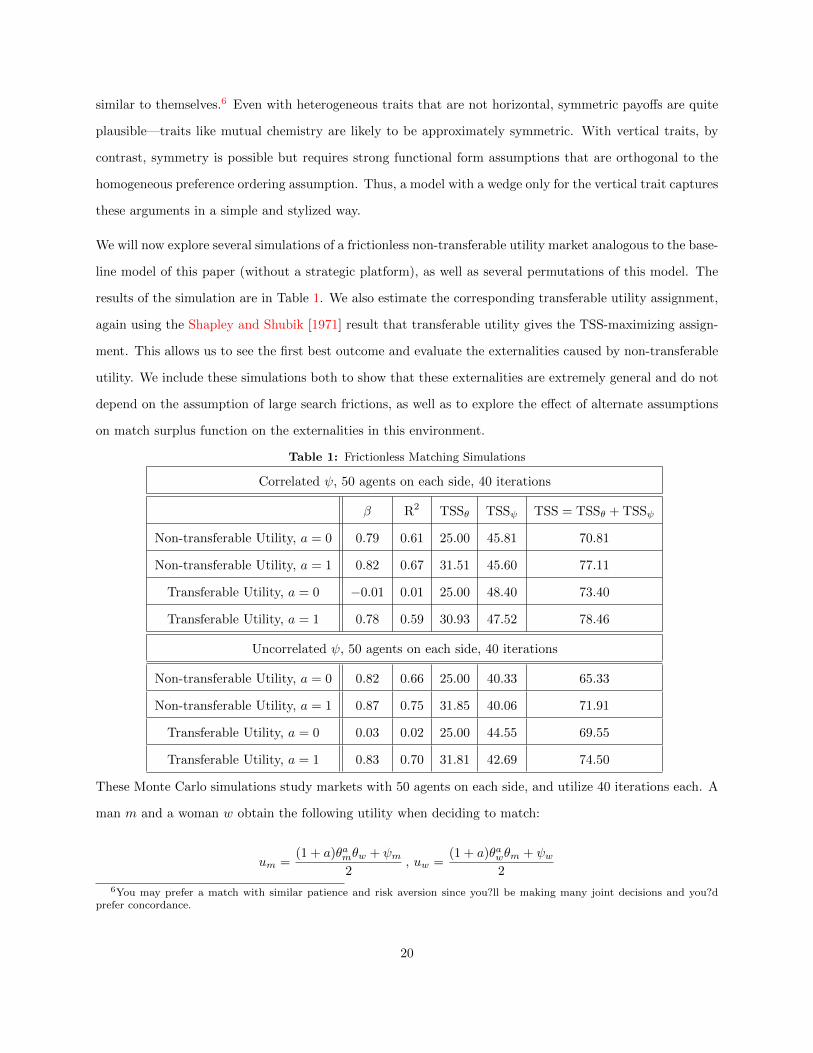
We will now explore several simulations of a frictionless non-transferable utility market analogous to the base-

line model of this paper (without a strategic platform), as well as several permutations of this model. The

results of the simulation are in Table 1. We also estimate the corresponding transferable utility assignment,

again using the Shapley and Shubik [1971] result that transferable utility gives the TSS-maximizing assign-

ment. This allows us to see the first best outcome and evaluate the externalities caused by non-transferable

utility. We include these simulations both to show that these externalities are extremely general and do not

depend on the assumption of large search frictions, as well as to explore the effect of alternate assumptions

on match surplus function on the externalities in this environment.

Table 1: Frictionless Matching Simulations

Correlated ψ, 50 agents on each side, 40 iterations

β R2 TSSθ TSSψ TSS = TSSθ + TSSψ

Non-transferable Utility, a = 0 0.79 0.61 25.00 45.81 70.81

Non-transferable Utility, a = 1 0.82 0.67 31.51 45.60 77.11

Transferable Utility, a = 0 −0.01 0.01 25.00 48.40 73.40

Transferable Utility, a = 1 0.78 0.59 30.93 47.52 78.46

Uncorrelated ψ, 50 agents on each side, 40 iterations

Non-transferable Utility, a = 0 0.82 0.66 25.00 40.33 65.33

Non-transferable Utility, a = 1 0.87 0.75 31.85 40.06 71.91

Transferable Utility, a = 0 0.03 0.02 25.00 44.55 69.55

Transferable Utility, a = 1 0.83 0.70 31.81 42.69 74.50

These Monte Carlo simulations study markets with 50 agents on each side, and utilize 40 iterations each. A

man m and a woman w obtain the following utility when deciding to match:

um =(1 + a)θamθw + ψm

2, uw =

(1 + a)θawθm + ψw2

6You may prefer a match with similar patience and risk aversion since you?ll be making many joint decisions and you?dprefer concordance.

20

Note that a is a parameter determining the supermodularity of the utility function. When a is zero, the utility

function is analogous to that of the baseline model, while a = 1 gives a vertical payoff component comprised

of the product of one’s own type and one’s match’s type. This means that higher types generate more utility,

and thus make matching high types to high types and low types to low types generates more surplus than

matching high and low types, all else equal. We’ll treat the case where ψm = ψw, as in the baseline model,

and also treat the case when they are independently drawn, dropping the symmetry assumption. Note that,

with supermodular utility, the vertical trait in fact exhibits symmetric payoffs, so we will be able to model

all four permutations of wedge and no-wedge over the two traits. ψ and θ are drawn from U [0, 1], and the

(1+a) term is a normalizing factor to account for the fact that, with the supermodular specification, utilities

will generally be lower since types are drawn from [0, 1] with an average of 0.5, so when a = 0, θamθw is 0.5

on average, while when a = 1, the match’s type is now multiplied by another draw from [0, 1], yielding 0.25

in expectation with random assignment. Defining an agent’s own type as (θ, ψ), match’s type as (θ′, ψ′),

and a match µ as µ(θ, ψ) = (θ′, ψ′), where µ1(θ, psi) = θ

′and µ2(θ, ψ) = ψ

′. With vertical traits, we are

interested in how aggressive the matching is along this trait, since we have predicted that it will be too high

with non-transferable utility. Since high types are mutually desirable and low types the opposite, we can

expect sorting along the vertical trait to induce assortative matching as per Becker [1973], with high types

using their attractiveness to ensure a high type match and low types being stuck with other low types. Thus,

more effort to match along the vertical trait should induce more correlation between own θ and match’s θ,

and in a sufficiently large market with only vertical sorting, E(µ1(θ, ψ)) = θ. Thus we will specify a simple

regression

µ1 = βθ + ε

and report the β and R2 vales. Additionally, we will report TSS, as well as TSSθ and TSSψ, with the

expectation that TSSψ and TSS should be higher for transferable utility and TSSθ should be weakly higher

for non-transferable utility.

Comparing non-transferable utility and transferable utility when a = 0 and ψs are correlated, the baseline

environment for the paper, we see that TSSθ is the same for both, as guaranteed by the above proposition—

with modular utility, the matching assignment doesn’t matter. However, in non-transferable utility agents

sort quite a bit on the vertical trait—high types get better matches, but those better matches come at a cost

to low types. The coefficient is relatively close to 1 and one’s own vertical type explains 60% of the variation

in match’s vertical type. This comes at a clear cost to TSSψ, which is much lower for the non-transferable

21

utility case, and thus TSS is also much lower, demonstrating the cost of these externalities.

Comparing non-transferable utility and transferable utility when a = 1 and ψs are correlated, we see sorting

on the vertical trait for both the first best and the non-transferable utility assignments since supermodularity

means that some assortation is desirable, but there is more sorting in theta with non-transferable utility and

worse assignments in ψ in terms of TSSψ. Now there is no wedge for either trait, so these externalities come

from rivalry, and rivalry is also weaker since the supermodularity means the costs imposed on low types are

scaled by their own type and are thus lower than the benefits accruing to high types. However, there is still

a modest loss in TSS due to rivalry.

Comparing non-transferable utility and transferable utility when a = 0 and ψs are uncorrelated, we again

see sorting on the vertical trait only for non-transferable utility assignments. Now there is a wedge for both

traits, so the no-transfers externalities should largely cancel. We see a large shortfall in TSSψ due to rivalry

with non-transferable utility, demonstrating the significance of this externality, especially with modular or

close to modular utility.

Finally, comparing non-transferable utility and transferable utility when a = 1 and ψs are uncorrelated,

we again see sorting on the vertical trait for both assignments. Now there is a wedge only for ψ, so the

externalities have opposite effects. The rivalry externality clearly dominates here, since there is still more

sorting along the vertical trait in the non-transferable utility case and less along ψ.

5 Optimal Monopolist Pricing

In this section, we will first present the non-distortionary pricing model, in which there are no externalities.

In particular, agents are identical. In the second and third subsection, we study the cases where there are

two types of vertically-differentiated agents. The difference between the later two subsections is the ability

of the firm to separate the two types of agents into separate platforms, each catering to only one type. In

the third subsection (the case where the firm cannot separate the types), we discuss some impediments to

separating the types into distinct platforms, and focus on two cases for the idiosyncratic matching shock

ψ: Case I, where there are small idiosyncratic shocks, and Case II, where ψ is distributed along a uniform

distribution on [0,m]. All cases considered in this section are for when agents’ types are perfectly observable

by the monopolist. Reader may refer to the online appendixes for this paper for further research on the case

where types are unobservable, and Cases III and IV, where we consider ψ to be distributed according to a

22

smooth distribution, and two-point distribution, respectively.7

5.1 Baseline Model With No Externalities

Consider the baseline model where there is only one vertical type and perfectly correlated matching shocks

ψ. This model with no externalities provide a baseline for the more complicated model later on, where

externalities are introduced through the α term and the tradeoff between choosing to match more aggressively

on the homogenous versus heterogeneous dimension. To solve for the steady-state equilibrium, note that the

monopolist acts a social planner who maximizes total surplus in the economy. In particular, the monopolist

will set prices to maximize the agent’s expected discounted utility of being on the platform. Now, note

that the only way prices affect the agent’s problem in the case with no externalities is through the agent’s

threshold ψ∗. For ease of exposition, since utility is additively separable, write the expected discounted

utility of agents as

EU(ψ∗) ≡ U − f − pD(ψ∗)

where U is the benefit from matching, D is the expected number of dates the agent goes on before leaving

the platform, p is the per-interaction price charged by the platform, and f is the fixed price. Recognizing

that prices affect the threshold ψ∗, we take first-order conditions with respect to ψ∗ to obtain

∂EU(ψ∗)

∂ψ∗= 0 =⇒ ∂U

∂ψ∗= p

∂D(ψ∗)∂ψ∗

=⇒ p = 0

Now, note that the monopolist profit function is given by

Π = 2{if +

∞∑t=0

δt+1ip(1− o)t} (14)

The profit function linearly increases in i, which implies that the monopolist optimally sets i = 1.8 This

fully characterizes the solution to the monopolist’s optimization problem for the case where there are no

externalities.

7This may be found at http://www.melatinungsari.com/research.html.8The profit function takes into account the cohort that entered the platform in steady state and follows them throughout

the entirety of their lives. This is in contrast to a similar (but incorrect way) of calculating profit, which is by calculating thesum of profits that is able to be extracted from the mass of agents in steady-state, regardless of the when they entered theplatform.

23

Proposition 7 In the model with no externalities and a differentiable F , the monopolist optimally sets

per-interaction fees to be zero, lets all agents in, and sets the fixed fee to extract all remaining surplus.

This result provides a benchmark for the case where there are no distortions caused by externalities imposed

by different types of agents on each other. In particular, the firm in acting as a social planner does not have

to correct the matching behavior of agents on the platform by charging a non-zero per-interaction price since

agent’s optimality conditions are already aligned with those of society.

5.2 Model with Externalities

Consider now a model where there are two types of agents, namely the studs (H types) and the duds (L

types). We will analyze two different cases—one in which the firm is able to separate the two types of

agents into different platforms and another where the firm is not able to separate the two types of agents

into distinct platforms. The firm may not be able to separate the two types of agents due to a variety of

reasons. For example, an online dating firm may specialize and operate only a single website, focusing on

aggressively advertising and managing the website. The firm may also face high fixed and operating costs to

operate more than one website, or may be faced with legal constraints that prevent them from segregating

the two types.

Another explanation as to why there could be two different platform configurations may simply be because

of the matching technology employed by the firm. To further illustrate this idea, consider the real-life online

dating platform eHarmony. This dating platform operates with a different matching technology than other

online dating platforms such as Match. The reason that eHarmony is different than Match because eHarmony

makes all of their users undergo a ‘personality quiz’ in which the users answer a long list of questions designed

to extract information about their characteristics and essentially, type. eHarmony then able to isolate a high

type from a low one, and limit the user’s choice set by only offering them access to agents who are similar

to themselves in types. Abstracting away from these details, we can model this as a two-platform model

where the firm fully observes the types of all agents and splits the population into two separate platforms

that cater to specific types.

This is in contrast to the matching technology employed by Match, where the website does not try and

extract more information about the types of the agents on the platform. In particular, the firm allows agents

to match freely with anyone while on the platform. The question now is whether or not the monopolist

24

would in fact, in the case where they are able to, operate two platforms instead of one. The answer to this

question is yes, under some unrestrictive assumptions on the distribution function F (.) of the idiosyncratic

match shock ψ. This result is intuitive but not trivial. In particular, the analysis is complicated by the fact

that the two platform configurations could have different outflow rates associated with the agents leaving

the platforms, and the fact that the proportion of studs on the platform, α, enters the analysis for the

one platform type. My result proves that under this model setup and assuming perfectly observable types,

the monopolist does strictly better by splitting the types into separate platforms following the strategy of

eHarmony than operating one platform like Match and letting all types freely search and match.

5.2.1 Firm Operates Two Platforms

Proposition 8 Suppose ψ is distributed according to a differentiable function F (.) with continuous and

bounded support. The monopolist profit is higher in the case where two platforms are operated (each catering

to only one type) than when only one platform is operated.

In the next subsection, we consider the case where the profit-maximizing monopolist is unable to separate

the two types into distinct platforms. As stated previously, this may be because the cost of doing so is

too high or plainly due to the matching technology employed by the firm (e.g. the online dating website

Match). The last important note regarding the previous proposition is the fact that it was proven by fixing

all the parameters in the model and also the endogenous α. The fact that the monopolist does better when

it operates two platforms rather than one for any value of α then implies that it is optimal to operate two

platforms under the equilibrium value of α.

5.2.2 Firm Operates Only One Platform

In this subsection, we consider the case where the monopolist firm can perfectly observe the types of the

agents, be it H or L. Given how real online dating platforms work, this is arguably a realistic setup.

The reason is primarily due to the fact that many online dating firms are usually able to extract enough

information from the agents on their types, be it through their self-proclaimed profiles on the website or

through an initial questionnaire. However, in reality, agents can still lie and misreport their type. This will

be addressed in more detail in the online appendix.

In solving for equilibrium, we focus on four cases for the idiosyncratic matching shock ψ. The first case is the

25

basic case with no idiosyncratic shocks. We then extend this to the case where the idiosyncratic matching

shocks are sufficiently ‘small’; that is when the shocks ψ are small relative to the size of the types θH and θL.

In this case, we are able to explicitly solve for the steady-state equilibrium. The second case that we study

is when ψ is uniformly distributed on the interval [0,m]. In this case, we obtain some partial equilibrium

results and also run numerical simulations to solve for a full steady-state equilibrium.9 Before proceeding to

these cases, we will first outline the monopolist’s problem in all entirety.

Monopolist’s Problem

We assume that the monopolist fully commits to a constant path of prices throughout time, charging {p∗ =

(p∗H , p∗L), f∗ = (f∗H , f

∗L)} in each period.

Definition 7 (Monopolist Profit) The firm’s expected profit in steady-state is

Πss ≡ 2 {iHfH + iLfL +

∞∑t=0

δt+1(pH iH(1− oH)t + pLiL(1− oL)t)}

This function can be thought of as the profit obtained by following the group of agents of type H and L

that entered in the steady-state until the end of their lives.10

By evaluating the summation, we simplify the expression for the steady state profit to obtain

Πss = 2{fH iH + fLiL +δiHpH

1− δ(1− oH(pH))+

δiLpL1− δ(1− oL(pH , pL))

} (15)

Given that types are perfectly observable, the monopolist is only concerned about the individual rationality

(participation) constraints. The optimization problem for the monopolist is defined as follows.

maxpH ,pL,fH ,fL

Πss(α(pH , pL), pH , pL)

9This a preview of the results for Case III and Case IV: in the third case, we look at when F is distributed according toa two-point mass distribution; that is, ψ is either γ > 0 with probability 1 − q or 0 with probability q. Here, we are not ableto provide any analytical results, but we provide numerical simulations for solving for equilibrium. The final case is when ψ isdistributed according to any smooth distribution. We are able to obtain analytical results for this case, where the results areslightly more restrictive than that of when ψ is uniformly distributed.

10As mentioned in a previous footnote, this is in contrast to another possible (but incorrect) way of expressing the profit,which would be to take into account all agents on the platform in steady-state, regardless of the time period in which theyjoined the platform:

Π = 2∞∑t=0

δt∑

j∈{L,H}{fj ij,t + µj,t pj}

26

s.t. (IRH) CH(α(pH , pL), pH)− fH ≥ 0

(IRL) CL(α(pH , pL), pH , pL)− fL ≥ 0

subject to the steady-state conditions in Definition 4.

The pricing problem is complicated by the fact that changes in prices affect not only one group of agents,

but also the interactions between the group and the other through the steady-state α. However, since types

are observable, the firm will extract all surplus from the agents, as proven below. This implies that the

pricing problem is equivalent to the planning problem in which the firm maximizes the total surplus of the

agents on the platform, only to charge prices to extract it all from them.

Proposition 9 In any steady state equilibrium with observable types, firm sets fixed prices f = {fH , fL}

and per-interaction prices p = (pH , pL) so that IRH and IRL bind.

Case I: No to Small Idiosyncratic Matching Shocks

Suppose, to begin, that there are no idiosyncratic shocks in this model. An agent of type i obtains the

following utility when she chooses to match with agent j:

ui(j) =θj

1− δ

An agent obtains the type of her match forever, which is discounted by the discount rate of δ. Agents are

risk-neutral and share the same discount rate with the firm. We can think of there being two steady-state

equilibrium: a pooling equilibrium where H and L types match not only amongst themselves but also with

each other, and a separating equilibrium with H types only match with other H types, and L types only

with other L types.

Since types are perfectly observable, the profit-maximizing monopolist will extract all surplus from the

agents by using a combination of per-interaction prices p = (pH , pL) and fixed fees f = (fH , fL). All agents

have the same outside option of obtaining zero utility when not on the platform. The individual rationality

constraints for each type will bind, giving

CH − fH = 0

CL − fL = 0

27

Since types are perfectly observable, we note that solving the monopolist problem is equivalent to solving

the social planner’s problem in which total social surplus is maximized. An agent’s strategy under this setup

is defined as

s∗i =

match with H

match with L and H

(16)

In equilibrium, since H determines whether or not a match forms, L’s only strategy will be whether or not

she will match with another L.

Under this setup, the total social surplus will be a function of all the types of agents on the platform. For

concreteness, suppose that there are only 4 agents in the market, with types H,H,L,L. There are only two

cases—the first in which H −H match and L−L match, and the other where two H −L matches form. In

the first case, the total amount of surplus that may be extracted is 2( θH1−δ ) + 2( θL1−δ ). In the second case, the

total amount is surplus that may be extracted is 2( θH1−δ + θL1−δ ). It is clear then that the total surplus that

may be extracted by the monopolist is the same for both cases; this implies that the monopolist does not

care about who matches with whom, but only about the total surplus that may be extracted. This result

obtains from the fact that the matching utility is additively separable (modular). Another important fact

to note is that an agent’s contribution to the total social surplus is his or her own type. This is due to the

fact that since an agent obtains his or her partner’s type in a marriage, each agent then contributes his or

her own type to the surplus.

We can now define the total social surplus on the platform. This is given by

Total Social Surplus (TSS) = µH

∞∑t=0

θH1− δ

δt(1− oH)tiH + µL

∞∑t=0

θL1− δ

δt(1− oL)tiL (17)

Note that prices are implicit in the expression of total social surplus. I can ignore explicit expressions of

prices since for any given expected discounted lifetime utility of being on the platform can be fully extracted

by the monopolist given a combination of prices. The prices only enter in the expression of total social

surplus in the outflows oH and oL, where higher prices would cause agents to be less picky and so, leave the

platform more quickly.

Now, we focus on the simplifying the expression for TSS by looking at optimal inflows. Since all agents agree

on the ranking of the types, H types are considered desirable by all other agents on the platform. Thus, iH

28

is optimally set to be 1. We need only characterize what the optimal iL is. In the following proposition,

we prove a strong and interesting result about this model, namely that given the setup and any range of

parameters, the monopolist will price per-interaction prices to extract all surplus from the agents and make

them leave in the first period. Also, given any range of parameters, the monopolist will choose to let all the

L types in, regardless of the value of θL.

Proposition 10 Consider the model with no idiosyncratic matching shocks. In the steady-state equilibrium,

the profit-maximizing firm will

1. Set iH = iL = 1.

2. Charge pH , pL sufficiently high to induce all agents to leave in the first period that they are on the

platform.

Proof. Consider the strategy where pH , pL is significantly high to induce all agents to leave the platform

immediately. In this strategy, the corresponding outflow rates for both types will be exactly 1. Given that

oH = oL = 1, we then note that the only way in which changing iL affects TSS is by affecting how quickly the

agents match, which is expressed through the outflow rates. Given that the outflow rates are held constant

at 1, under this pricing strategy, the TSS becomes an increasing linear function in iL, implying that the firm

optimally sets iL = 1. Now, all that remains to be shown is the optimality of charging prices that make all

agents leave immediately.

By evaluating the summation in (17), I can write the expression as

TSS = µH(iHθH

(1− δ)(1− δ(1− oH))) + µL(

iLθL(1− δ)(1− δ(1− oH))

) (18)

By taking derivatives, I note that

∂TSS

∂oH,∂TSS

∂oL≥ 0

which implies that the optimal pricing strategy is then to set oL = oH = 1. Under this pricing strategy, we

have shown earlier that the corresponding optimal inflows are iL = iH = 1.

There is an intuitive interpretation for this result in terms of the discount rate δ. Consider three cases for

the discount rate: δ = 1, δ = 0, and δ ∈ (0, 1). In the case where δ = 1, any pricing strategy that the firm

sets will give the same TSS, since agents essentially weight each period the same. In the case where δ = 0,

29

the model reduces to that of a one-period model, where it is obviously optimal for the profit-maximizing

monopolist to extract all surplus by charging the highest possible per-interaction prices. For any δ ∈ (0, 1),

note that TSS is strictly decreasing in the the number of periods that the agents stay on the platform. This

being, the pricing strategy that forces everyone to leave immediately gives a higher TSS than any other

pricing strategy. Thus, the optimal pricing strategy for the firm is to set per-interaction prices sufficiently

high to induce all agents to leave in the first period.

Now, we would like to make strides towards understanding the model where the idiosyncratic shock is

sufficiently small. We have already shown what the steady-state equilibrium looks like in the context of no

idiosyncratic shocks. What happens when these shocks are small, i.e. when the support of the distribution

of ψ is small? It turns out that the result for when the shocks are small relative to the size of the types

(θH , θL) is the same as in the case where there are no shocks for a range of parameters that occurs with

positive probability. A sufficient but not necessary condition for the shock ψ being small is θLm ≥

δ1−δ .

Proposition 11 Suppose ψ ∈ [0,m]. Then for parameterizations such that θLm ≥

δ1−δ , the profit-maximizing

monopolist

1. Sets iH = iL = 1.

2. Charge pH , pL sufficiently high to induce all agents to leave in the first period that they are on the

platform.

Proof. Consider again the expression for total social surplus. Since the matching utility is additively

separable, we may write the total social surplus as

Total Social Surplus (TSS) =∑

j∈{L,H}

µj

∞∑t=0

( θj1− δ

+E(ψ | j matches)

1− δ

)δt(1− oj)tij (19)

where µj is the mass of type θj on the platform. By the same reasoning as in the previous proposition, given

the pricing strategy where the firm sets per-interaction prices sufficiently high to force everyone to match in

the first period, it is clear that iH = iL = 1. Now, consider two pricing scenarios:

1. Per-interaction prices are set sufficiently high to force everyone to match in the first period and oH =

oL = 1.

2. Per-interaction prices are set such that ∃ some measure λH of H agents and λL of L agents that wait

on the platform and do not immediately match.

30

By assumption of the bounded support of ψ, the worst draw that any agent can obtain is any period is ψ = 0

and the best is ψ = m. Thus, we can bound the total social surplus from scenario 1 by the case where agents

obtain a shock of ψ = 0 in each period:

TSS1 ≥ µH(θH

1− δ) + µL(

θL1− δ

)

Note that the proportion (1−λH) and (1−λL) of H and L agents, respectively, we can write the total social

surplus in scenario 2 as:

TSS2 = λHµH TSS2,H + λLµL TSS2,L + (1− λH)µH TSS1,H + (1− λL)µL TSS1,L

where TSSn,j is the total surplus obtained from j ∈ {L,H} in case n ∈ {1, 2}.

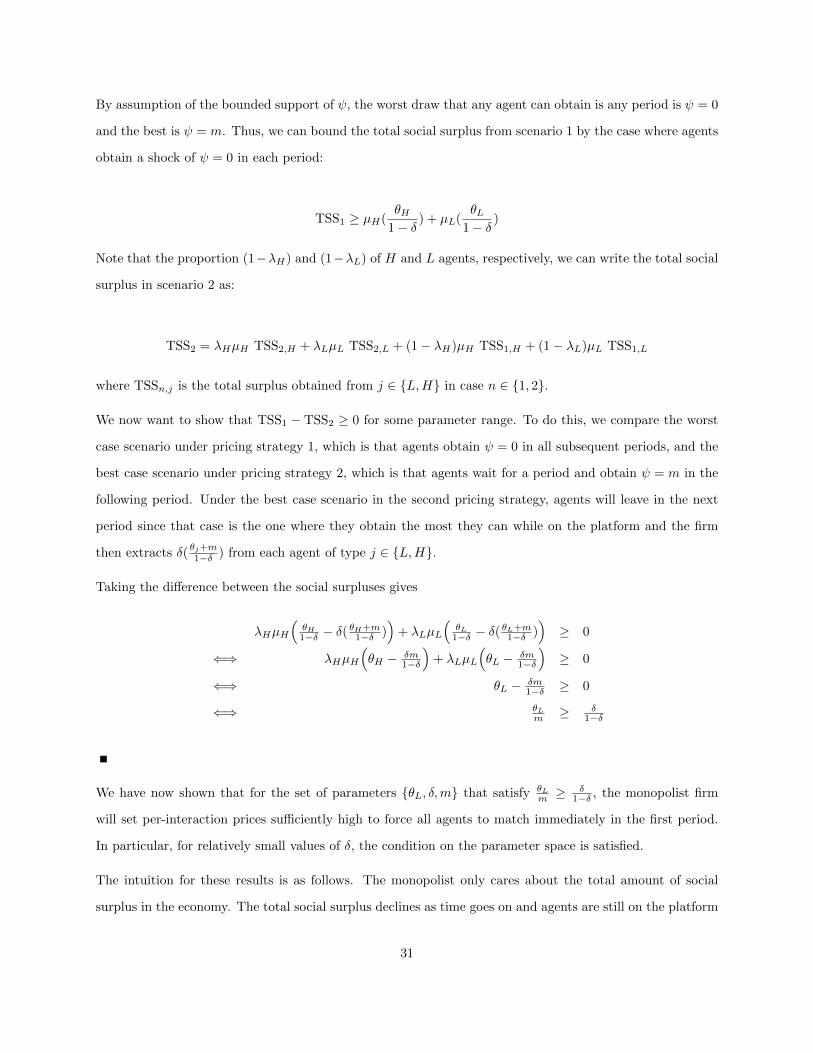
We now want to show that TSS1 − TSS2 ≥ 0 for some parameter range. To do this, we compare the worst

case scenario under pricing strategy 1, which is that agents obtain ψ = 0 in all subsequent periods, and the

best case scenario under pricing strategy 2, which is that agents wait for a period and obtain ψ = m in the

following period. Under the best case scenario in the second pricing strategy, agents will leave in the next

period since that case is the one where they obtain the most they can while on the platform and the firm

then extracts δ(θj+m1−δ ) from each agent of type j ∈ {L,H}.

Taking the difference between the social surpluses gives

λHµH

(θH1−δ − δ(

θH+m1−δ )

)+ λLµL

(θL1−δ − δ(

θL+m1−δ )

)≥ 0

⇐⇒ λHµH

(θH − δm

1−δ

)+ λLµL

(θL − δm

1−δ

)≥ 0

⇐⇒ θL − δm1−δ ≥ 0

⇐⇒ θLm ≥ δ

1−δ

We have now shown that for the set of parameters {θL, δ,m} that satisfy θLm ≥

δ1−δ , the monopolist firm

will set per-interaction prices sufficiently high to force all agents to match immediately in the first period.

In particular, for relatively small values of δ, the condition on the parameter space is satisfied.

The intuition for these results is as follows. The monopolist only cares about the total amount of social

surplus in the economy. The total social surplus declines as time goes on and agents are still on the platform

31

by a factor of δ in each period. This being, the monopolist will want to force agents to match immediately

while on the platform unless there is a non-zero probability of agents obtaining a sufficiently high draw ψ,

which will improve their utility and so increase the amount of surplus that can be extracted from them.

In the case where the idiosyncratic matching shock ψ is small relative to the size of the types θH and θL,

the incentives for the monopolist to let agents stay on the platform for long are corresponding small. In

particular, with both agents and the monopolist valuing the future very little (implying low values of δ),

there is no incentive for either side to stay longer on the platform when the benefit of waiting on the platform

for a better ψ is small.

One natural question to ask now is whether the firm charges different per-interaction and fixed prices to the

studs and duds under the parameter range where the pricing strategy of charging sufficiently high prices to

induce agents to match immediately is implemented. What is observed is that since the monopolist firm

lets all agents in to the platform and outflow rates for both studs and duds are exactly 1, the probability of

meeting a stud or dud is exactly (denoted α) is also exactly 12 . Since the chance of meeting a stud is the same

for both types of agents, and per-interaction prices are set to induce both agents’ acceptance thresholds to

be 0 (agents marry their first match), agents expected lifetime utility of being on the platform is the same

regardless of type. Thus, we obtain the following result that the profit-maximizing monopolist charges the

same fixed prices to both H and L types, despite the fact that types are observable.

Proposition 12 Suppose θLm ≥

δ1−δ and types are perfectly observable. In the steady-state equilibrium, the

profit-maximizing monopolist sets sufficiently high per-interaction prices p∗H , p∗L so that all agents match and

exit in the first period and f∗H = f∗L.

One fact to note is that although the fixed prices are the same for both types of agents, the optimal per-

interaction prices may or may not be the same. In particular, the only restriction on per-interaction prices is

that they have to be sufficiently higher than a certain threshold. After they reach the threshold, whether or

not the per-interaction prices for studs and duds are the same is inconsequential. However, since agents do

not actually pay the per-interaction prices in the first period that they are searching on the platform if they

marry in the first period, this optimal contract essentially does not differentiate between types since it only

consists of fixed prices. The per-interaction prices for both types are just set to provide strong incentives

(i.e. force you) to immediately marry the first person you go on a date with.

Case II: The Idiosyncratic Matching Shock ψ is Uniformly Distributed on [0,m]

Now, we study the case when the random matching shock ψ is draw from a uniform distribution on [0,m].

32

In particular, we would like to elaborate on the assumptions that the following proposition makes. The facts

to note are the following:

1. In studying the case where the shocks are uniformly distributed, we fix the pricing strategy for the H

types. This implies that the analysis done is a partial equilibrium analysis. Fixing the pricing strategy

for the H types is necessary to keep the H type optimality conditions the same. This is because by

fixing the pricing strategy, we are able simplify the problem greatly due to the complexities that arise

from the fixed point analysis with the proportion of studs on the platform, α.

2. We assume that iL ∈ (0, 1); that is, that the monopolist is letting in a nonzero proportion of the L

types. In practice, to check whether or not the solution we obtain is optimal, we may compare the

profit obtained from the equilibrium in the proposition with the one where the firm lets no duds in

(i.e. iL = 0).

3. We also assume that for a fixed pL that ψ∗L(L) ∈ (0,m). This is to ensure that prices have a bite; that

is, changing prices will actually affect how the L type optimizes. For example, if the threshold were at

0, L types are already choosing to always match with other L types and so prices have no effect on the

threshold. The duds would ideally like to lower their threshold with an increased pL but are unable to

do so. In the case where ψ∗L(L) = m, L types never match with other L types anyway, and so prices

have no effect on the thresholds.

Proposition 13 Suppose 0 < iL < 1, fix iH , pH and pL, suppose F is the uniform distribution with support

[0,m], and ψ∗L(L) ∈ (0,m). The firm can strictly increase profits by increasing both iL and pL by ε > 0.

Corollary 8 Suppose the conditions in the previous proposition hold. In equilibrium, if the firm chooses to

let any L types onto the platform, it will let all of them in (i.e. set iL = 1).

Note that this corollary does not state whether it is always optimal to let any L types in (i.e. iL > 0) or

whether pL > 0. In particular, it may be that if θH − θL is very large (or rather if the L type is very ‘weak’),

then the optimal choice for iL may be to set iL = 0 to eliminate the negative externality that L imposes on

H.

Despite the small number of primitives in this model, analytical results are difficult to obtain. This is primar-

ily due to two factors, the first being that the the effects of perturbations in the model depend on the exact

specification of the distribution function of ψ, F (.). The second reason is because of the fixed point nature

of the equilibrium. In particular, even though agents take the proportion of high types on the platform,

33

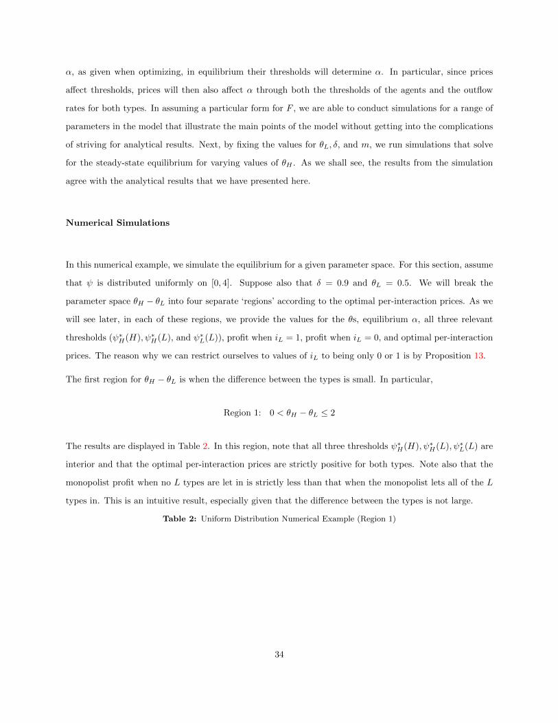
α, as given when optimizing, in equilibrium their thresholds will determine α. In particular, since prices

affect thresholds, prices will then also affect α through both the thresholds of the agents and the outflow

rates for both types. In assuming a particular form for F , we are able to conduct simulations for a range of

parameters in the model that illustrate the main points of the model without getting into the complications

of striving for analytical results. Next, by fixing the values for θL, δ, and m, we run simulations that solve

for the steady-state equilibrium for varying values of θH . As we shall see, the results from the simulation

agree with the analytical results that we have presented here.

Numerical Simulations

In this numerical example, we simulate the equilibrium for a given parameter space. For this section, assume

that ψ is distributed uniformly on [0, 4]. Suppose also that δ = 0.9 and θL = 0.5. We will break the

parameter space θH − θL into four separate ‘regions’ according to the optimal per-interaction prices. As we

will see later, in each of these regions, we provide the values for the θs, equilibrium α, all three relevant

thresholds (ψ∗H(H), ψ∗H(L), and ψ∗L(L)), profit when iL = 1, profit when iL = 0, and optimal per-interaction

prices. The reason why we can restrict ourselves to values of iL to being only 0 or 1 is by Proposition 13.

The first region for θH − θL is when the difference between the types is small. In particular,

Region 1: 0 < θH − θL ≤ 2

The results are displayed in Table 2. In this region, note that all three thresholds ψ∗H(H), ψ∗H(L), ψ∗L(L) are

interior and that the optimal per-interaction prices are strictly positive for both types. Note also that the

monopolist profit when no L types are let in is strictly less than that when the monopolist lets all of the L

types in. This is an intuitive result, especially given that the difference between the types is not large.

Table 2: Uniform Distribution Numerical Example (Region 1)

34

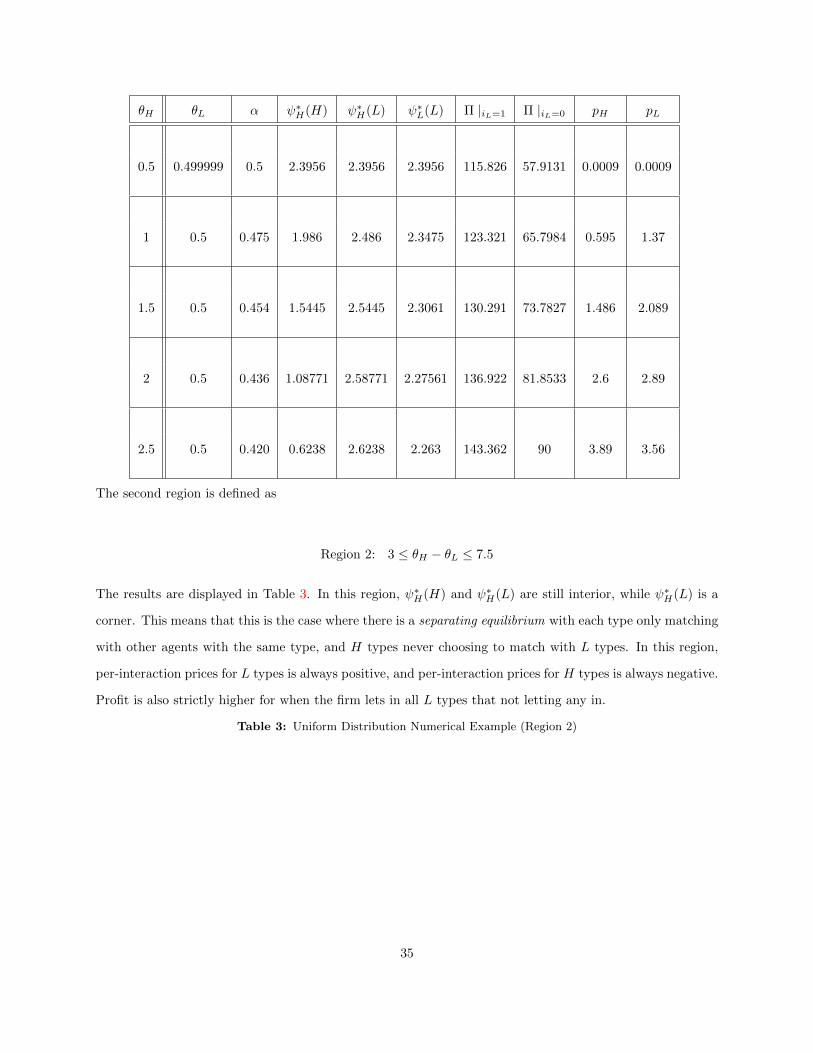
θH θL α ψ∗H(H) ψ∗H(L) ψ∗L(L) Π |iL=1 Π |iL=0 pH pL

0.5 0.499999 0.5 2.3956 2.3956 2.3956 115.826 57.9131 0.0009 0.0009

1 0.5 0.475 1.986 2.486 2.3475 123.321 65.7984 0.595 1.37

1.5 0.5 0.454 1.5445 2.5445 2.3061 130.291 73.7827 1.486 2.089

2 0.5 0.436 1.08771 2.58771 2.27561 136.922 81.8533 2.6 2.89

2.5 0.5 0.420 0.6238 2.6238 2.263 143.362 90 3.89 3.56

The second region is defined as

Region 2: 3 ≤ θH − θL ≤ 7.5

The results are displayed in Table 3. In this region, ψ∗H(H) and ψ∗H(L) are still interior, while ψ∗H(L) is a

corner. This means that this is the case where there is a separating equilibrium with each type only matching

with other agents with the same type, and H types never choosing to match with L types. In this region,

per-interaction prices for L types is always positive, and per-interaction prices for H types is always negative.

Profit is also strictly higher for when the firm lets in all L types that not letting any in.

Table 3: Uniform Distribution Numerical Example (Region 2)

35

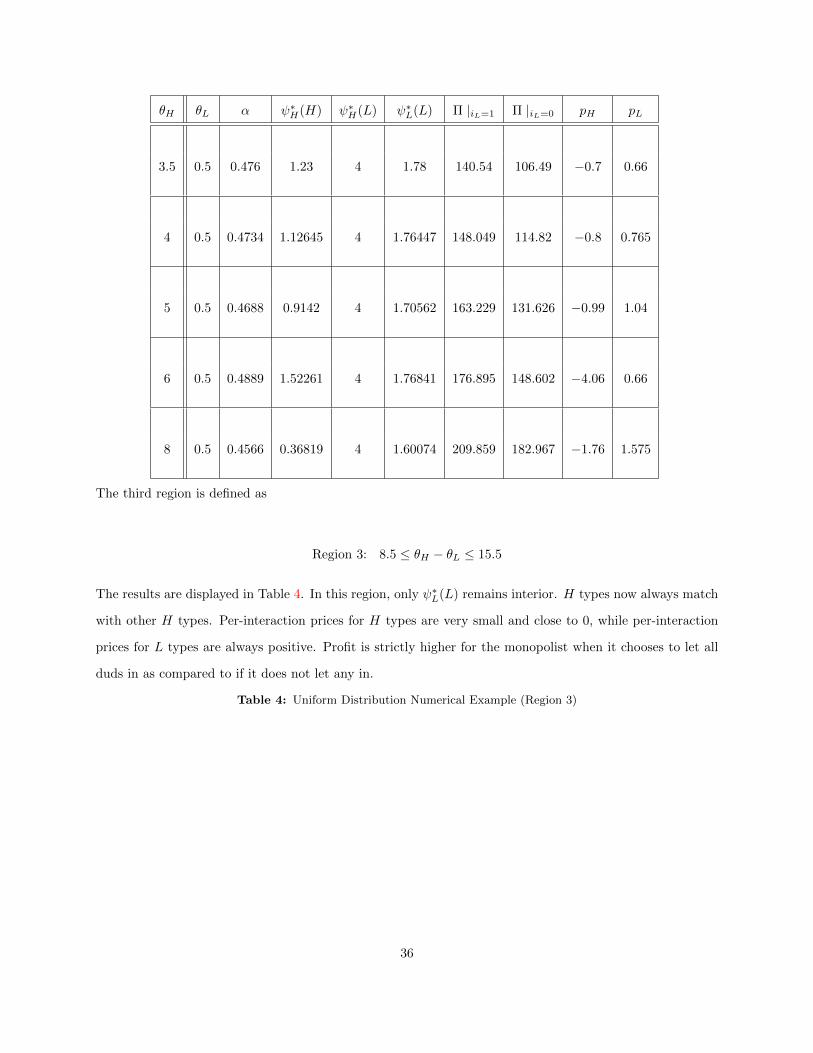
θH θL α ψ∗H(H) ψ∗H(L) ψ∗L(L) Π |iL=1 Π |iL=0 pH pL

3.5 0.5 0.476 1.23 4 1.78 140.54 106.49 −0.7 0.66

4 0.5 0.4734 1.12645 4 1.76447 148.049 114.82 −0.8 0.765

5 0.5 0.4688 0.9142 4 1.70562 163.229 131.626 −0.99 1.04

6 0.5 0.4889 1.52261 4 1.76841 176.895 148.602 −4.06 0.66

8 0.5 0.4566 0.36819 4 1.60074 209.859 182.967 −1.76 1.575

The third region is defined as

Region 3: 8.5 ≤ θH − θL ≤ 15.5

The results are displayed in Table 4. In this region, only ψ∗L(L) remains interior. H types now always match

with other H types. Per-interaction prices for H types are very small and close to 0, while per-interaction

prices for L types are always positive. Profit is strictly higher for the monopolist when it chooses to let all

duds in as compared to if it does not let any in.

Table 4: Uniform Distribution Numerical Example (Region 3)

36

θH θL α ψ∗H(H) ψ∗H(L) ψ∗L(L) Π |iL=1 Π |iL=0 pH pL

9 0.5 0.444895 0 4 1.52931 225.349 200.323 0.03 1.98

10 0.5 0.447795 0 4 1.46619 241.362 217.778 0.01 2.25

15 0.5 0.46 0 4 1.18132 321.698 306.217 −0.06 3.5

20 0.5 0.47 0 4 0.907 402.426 396 −0.05 4.76

The fourth and last region is defined as

Region 4: 24.5 ≤ θH − θL ≤ 44.5

The results are displayed in Table 5. This is the region for which the difference in types, θH−θL, is extremely

large. In particular, note that the monopolist profit when no L types are let onto the platform is strictly

higher than the monopolist profit when all L types are let onto the platform. The L type is so bad that the

negative effects of their presence on the platform on the H types greatly outweighs the benefit that L types

get of being on the platform and matching only with each other. In this region, no L types will be let onto

the platform and the monopolist charges 0 to all H types, which is consistent with the baseline model with

no externalities.

Table 5: Uniform Distribution Numerical Example (Region 4)

37

θH θL α ψ∗H(H) ψ∗H(L) ψ∗L(L) Π |iL=1 Π |iL=0 pH pL

25 0.5 0.48 0 4 0.649 483.482 486 −0.11 6.04

30 0.5 0.488335 0 4 0.390108 564.819 576 0 7.35

45 0.5 0.41874 0 4 2.03219 793.523 846 0 0

Note that since everyone on the platform prefers to match with H types, the monopolist values the studs and

so always lets all H types in; that is, iH = 1. From these numerical examples using the uniform distribution,

we can make the following observations:

1. As θH −θL → 0, per-interaction prices are optimally set to 0, fixed prices are set so that the individual

rationality constraints bind, and the firm lets both types into the platform (iH = iL = 1).

2. As θH − θL →∞, the firm will not let any iL in (iL = 0).

3. Optimal per-interaction prices for L types is always strictly positive (pL > 0).

As we have seen through the four different regions, each region has different sign combinations of optimal

per-interaction prices. In the first region, when the difference θH − θL is very small, the monopolist firm

will choose to charge pH , pL > 0. In the second region, the monopolist charges pH < 0, pL > 0. In the third

region, the monopolist charges pH close to 0 and pL > 0. In the last region where the difference in types is

extremely large, the monopolist chooses to not let in any L types and sets pH = 0.

The intuition for my results can be obtained by considering the externalities exerted by both types of the

agents onto each other and within their own type. First of all, note that studs are valuable to everyone; this

includes the monopolist, duds, and other studs. The H types are very valuable to the monopolist since the

monopolist wants to extract their surplus θH that they bring to any marriage, if it forms. The H type is

valuable to other agents on the platform since the all agents prefer to match with other H types. Secondly,

note that the presence of too many L types negatively affects the H types, since more duds will lead to

a lower α, which in turns decreases the expected lifetime utility of H types being on the platform. The

firm can observe these externalities and can use per-interaction prices to distort the optimization problem

38

of the agents by making agents more or less picky. As we will see, there is a trade off between the gain the

monopolist obtains from the L types by letting them match on the platform and the loss it incurs from the

H types at the same time from having other L types on the platform and facing a lower α. Consideration

is also given to balancing these externalities with those that occur in between agents of the same type, as in

Region 1.

Considering these externalities, we can analyze the effects of type differences and externalities on per-

interaction pricing. Let ∆ ≡ (θH − θL).

1. For any value of ∆, the firm optimally charges the duds a positive per-interaction price. This is

because H types are strictly preferred by the firm and L types can be seen as ‘clogging up the system’,

even when their type is not too different from that of studs. The monopolist can push the L quicker

through the system by charging a positive per-interaction price, which increases as the difference in

types increases. In particular, having even a small positive per-interaction price for the duds, pL,

decreases the time that duds spend on the platform, which in turn will increase α, the proportion of

studs on the platform. By Proposition 5, an increase in α increases the happiness of the studs, which

allows the firm to extract more in surplus. In any case, the fact that pL > 0 is unsurprising, since I

have already proven that this is the case in Case III where F , the distribution of ψ, is any smooth

distribution.

2. When ∆ is small (Region 1), a positive price pH would increase the chance that L will match with H

types since it lowers H’s matching thresholds and makes them less picky. This benefits the L types.

3. When ∆ is small (Region 1), a positive price pH would also increase the chance that H types match

with other H types. An increased per-interaction price lowers H’s matching threshold of dating other

H types. This benefits the monopolist, who cares about extracting all the surplus it can, and would

very much like to extract as many θH terms as possible.

4. When ∆ is not too large (Region 2), note that ψ∗H(L) = 4, which is a corner solution. The other

two thresholds, ψ∗L(L) and ψ∗H(H), are interior. The fact that ψ∗H(L) = 4 implies that studs never

marry duds. In this case, the monopolist loses out on all surplus that could have resulted from all

of the stud-dud marriages that could have occurred. The firm makes up for by charging negative

per-interaction prices to studs and increasing their pickiness. This causes them to stay on the platform

longer to search and in turn, increases the proportion of studs on the platform, α. By Proposition 5,

this makes the studs happier, which allows the firm to extract more in surplus from them. We can

39

also relate the results from Region 2 to the externalities found in Shimer and Smith [2001]. There are

two externalities in play, the thick-market externality and the congestion externality. First of all, the

thick-market externality implies that studs do not internalize the fact that by leaving the platform,

they decrease α, which negatively affects other studs. Secondly, since studs never marry duds, an

increase in α negatively affects the duds, since the duds will have to waste time and money by going

on many dates with agents who will never marry them. The monopolist then weighs the benefit to the

studs of having a higher α to the loss incurred by the duds with having more studs on the platform

and finds that the thick-market externality is stronger than the congestion externality. This being, the

monopolist will set pH to be negative to increase α.

5. When ∆ is large (Region 3), note that ψ∗L(L) is interior but ψ∗H(H) and ψ∗H(L) are both corner

solutions. This means that studs always marry other studs and never marry duds. In this region,

the firm’s instrument of per-interaction prices have no bite with the studs, since their thresholds are

both already at the corner. In particular, since ∆ is large, the firm is not able to charge a very high

positive pH to lower the threshold ψ∗H(L), and is not able to charge a very low negative price pH to

increase ψ∗H(H). This implies that the equilibrium pricing strategy for the studs consists of a range

of per-interaction prices pH , where this range also includes the non-distortionary zero. The condition

that this equilibrium range must satisfy is that the price pH is not too extreme—if pH is either too

low or too high, the thresholds for the studs will change.

6. When ∆ is extremely large (Region 4), L types are not let onto the platform. This reduces to the

baseline model with no externalities studied in Section 4.

6 Conclusion

In this paper, we presented a two-sided matching model with non-transferable utility where agents have

preferences over multiple dimensions. We found two previously unstudied matching externalities that result

from our framework, which we named the rivalry and no-transfers externality. The rivalry externality is an

externality that exists due to the fact that agents make tradeoffs between all of the different dimensions of

characteristics that they match on. In particular, our main finding is that agents will match too aggres-

sively on homogenous traits versus heterogenous traits. The no-transfers externality exists due to the fact

that utility is non-transferable and so agents are not able to resolve any externalities privately by bargain-

40

ing. We showed, using simulations, that these externalities are robust to markets with no search frictions,

supermodular utility functions instead of modular, and uncorrelated idiosyncratic matching shocks.

Given these interesting externalities, we also studied how a profit-maximizing monopolist platform would

price its services. If the firm is able to operate two separate platforms, we showed that it will fully separate

the two types and the pricing equilibrium will be non-distortionary. For the case when the firm operates only

one platform, we studied two different scenarios for the idiosyncratic matching shock ψ. The first case was

when there are no to small idiosyncratic matching shocks and the second was when ψ uniformly distributed

on [0,m]. We characterized ‘separating’ equilibria where studs only marry other studs and duds only marry

other duds and ‘pooling’ equilibria where studs and duds intermarry. Assuming the monopolist charges a

two-part tariff and types are perfectly observable, we also found parameterizations where the optimal pricing

strategy was to charge distortionary (non-zero) per-interaction prices to correct for the externalities on the

platform.

In general, this paper has two main contributions. The first is that it provides a way to understand the

externalities and tradeoffs faced by agents in realistic matching models where agents have preferences over

multiple dimensions, instead of just one. For example, if one considers the market for medical residents in

the U.S. (i.e. The Match), our results show that from a social planner’s perspective, medical residents in

this market match too aggressively on rankings of the hospitals and not aggressive enough on geographical

locations. This fact may have prescriptive consequences as the authorities can correct for this behavior by

providing incentives to lessen the tradeoff between matching on heterogenous (e.g. geographical location) and

homogenous (e.g. ranking) traits. The second contribution of this paper is that it provides a way to embed a

two-sided matching framework with search into a pricing model. Even though our model is mathematically

difficult to analyze, it provides a foundation for future work in building more tractable models that study

pricing and externalities resulting from matching behavior on two-sided platforms.

41

Appendix

Proposition (2)

Proof.

Recall the Bellman Equation

Vi(ψ | j) = max{θj + ψ

1− δ, δ(αVi(ψ | H) + (1− α)Vi(ψ | L))− pi} (20)

When deciding whether to match with agent j, agent i takes prices and also the function Vi(ψ | ¬j) as given.

Thus, we may rewrite the above equation as

Vi(ψ | j) = max{θj + ψ

1− δ, αVi(ψ | j) + c} (21)

where, assuming with no loss of generality that j = H,

α = δα

and

c = δ(1− α)Vi(ψ | L)− pi

where both c and α are constants. To prove the fixed point is unique, I first show that the two conditions

of the Blackwell Sufficient Conditions Theorem is proven. This will show that T is a contraction. The

contraction mapping theorem will then show that T has a unique fixed point.

The first is monotonicity. Let Vi(ψ | j) ≤Wi(ψ | j). Then

T (Vi(ψ | j)) = max{ θj+ψ1−δ , αVi(ψ | j) + c}

≤ max{ θj+ψ1−δ , αWi(ψ | j) + c}

≤ T (Wi(ψ | j))

The second sufficient condition is discounting. Let a ≥ 0 and f ∈ B(X). Then

42

T ((Vi(ψ | j) + a)(x)) = max{ θj+ψ1−δ , α((Vi + a)(ψ | j) + c}

= max{ θj+ψ1−δ , αVi(ψ | j) + αa+ c}

≤ max{ θj+ψ1−δ , αVi(ψ | j) + c}+ αa

= T (Vi(ψ | j)) + αa

Proposition (3)

Proof.

Recall that

Ci =θH + ψ∗i (H)

1− δ=θL + ψ∗i (L)

1− δ

at the interior thresholds. Since θH − θL > 0, we get that

ψ∗i (L)− ψ∗i (H) = θH − θL > 0

Proposition (4)

Proof. Note that since

Ci =θH + ε∗i (H)

1− δ=θL + ε∗i (L)

1− δ(22)

proving that CH > CL is the same as showing that

ψ∗H(j) > ψ∗H(j) ∀j ∈ {L,H}

Thus, proving (4) proves (3). From a previous proposition, we know that ∀i ∈ {L,H}, ψ∗i (L) ≥ ψ∗i (H),

which implies that, for a fixed i,

43

P (i matches with H) = 1− F (ψ∗i (H)) > P (i matches with L) = 1− F (ψ∗i (L))

Since θH > θL, H can always pretend to be L, mimic the strategy of L(ψ∗L) and obtain CL. By the optimality

of ψ∗, it must be that

CH(ψ∗H) > CH(ψH)

That is, H must obtain strictly more more he uses the optimal ψ∗ strategy compared to any other possible

strategy. This gives that

CH(ψ∗H) > CH(ψH) ≥ CL(ψ∗L) for any other strategy ψH

I have demonstrated that CH(ψ∗H) ≥ CL(ψ∗L), which implies that ψ∗H(H) ≥ ψ∗L(H). Now I must show that

CH(ψ∗H) 6= CL(ψ∗L). I have previously shown that

ψ∗H(L) > ψ∗H(H) ≥ ψ∗L(H)

Consider the event where ψ ∈ (ψ∗H(H), ψ∗H(L)) and an agent of type i who meets an H type agent. If i = H,

the pair will form a match and leave since ψ > ψ∗H(H). If i = L, L will want to form a match withy H

because ψ > ψ∗L(H) , but H will not want to form a match sine ψ < ψ∗H(L). This means that a match will

not form.

Thus, in the interval ψ∗H(H), an agent of type H does strictly better since in the case where he meets another

H agent, he obtains

uH(H | ψ) > CH(ψ∗H) ≥ CL(ψ∗L)

whereas L gets CL since ψ > ψ∗L(H). For all other realizations of ψ, i.e. (ψ∗H(H), ψ∗H(L))c, the expected

utility of H and L are the same. Thus, the expected utility of H is strictly greated than the expected utility

of L over the entire support of ψ.

Corollary (3)

44

Proof. As I have shown in the previous proof, proving that CH > CL is equivalent to proving this corollary.

The corollary trivially follows.

Proposition (5)

Proof.

There are four claims to prove. (1) is easy to see from the Bellman equation from which the thresholds are

derived:

Vi(ψ | j) = max{θj + ψ

1− δ, δ(αVi(ψ | H) + (1− α)Vi(ψ | L))− pi} (23)

The price enters the optimization problem of the agents as a negative constant, proving the result. From

(23), note that both terms in the Bellman equation are strictly increasing in δ, proving (2). I proceed with

proving (3). Note that proving (3) is equivalent to proving (4) by (22).

Fix an agentH. There are then two cases. The first is whenH never matches with L (separating equilibrium).

This may be due to a variety of reasons. Some explanations include the difference in their types (θH − θL)

being extremely large, or that the draw ψ was very bad. Whatever it is, an increase in α in this first case

obviously increases the continuation value for H since it increases the probability that H meets another H,

which then increases the chance that H will find a match in any given period.

The second case is when H matches with L. Consider now an αold and a corresponding CH,old with strategies

ψ∗H,old = {ψ∗H(H, old), ψ∗H(L, old)}. Let αnew > αold. Consider a strategy

ψ∗H,new = {ψ∗H(H,new), ψ∗H(L,new)}

where ψ∗H,new = ψ∗H,old for all agents in the proportion αold and ψ∗H(H,new) = ψ∗H(H, old) for all ‘new’ agents

in the proportion αnew − αold. In words, this means that this new strategy is the same for the proportion

of agents who were and currently are H types and is different for the proportion of agents who are now H

instead of being L types before. For the proportion of agents who are H types now instead of L, this new

strategy employs the cutoff strategy that H would use when faced with L agents in the past.

This would imply that from the proportion αold, we get that

45

CH,new,αold= CH,old

and from the new proportion αnew − αold, we have that

CH,new,αnew−αold= (αnew − αold)uH(L | ψ∗H(L, old))

This gives that

CH,new = CH,new,αnew−αold+ CH,new,αold

> CH,old

which is true because uH(L | ψ∗H(L, old)) ≥ 0 and αnew−αold > 0. By the definition of optimality, it is true

that the optimal threshold strategy ψ∗H does strictly better than any other strategy for the agent. Thus,

CH(ψ∗H) > CH(ψ) for any other ψ

Thus, as α increases, the continuation value CH increases as well.

Proposition (8)

Proof. Fix α, iH , iL, and all the parameters in the model. In the one platform case, there are three thresholds

of interest: ψ∗H(L), ψ∗L(L), and ψ∗H(H). All three thresholds are functions of α, which is the proportion of

studs on the platform. In the two platform case there are only two thresholds of interest, one for each of the

platforms. We define these two thresholds to be ψ∗H and ψ∗L. In particular, in the separate platforms case the

studs only need to worry about their thresholds to marry another studs, and the same goes for the duds. To

simplify the analysis, we equalize the outflow rates for both types on both configurations of platforms. There

are two main reasons for doing so. The first is to make the problem tractable by simplifying the calculations

done later in the proof. The second is because we would like to utilize optimality conditions to aid in the

proof. To see this, consider the outflows for the one platform case that are a result of the optimal pricing

strategy of the firm and consider an arbitrary pricing strategy for the two platform case that gives outflows

for both types exactly equal to that of the one platform case. If we can show that even under this arbitrary

46

pricing strategy the monopolist profit for operating two separate platforms is higher than that of operating

a single platform, then optimality conditions dictate that the optimal pricing strategy for operating two

separate platforms will necessarily do at least as well.

Now, recall that the outflow rate for H types while on the mixed platform is

oH,one platform = α(1− F (ψ∗H(H))) + (1− α)(1− F (ψ∗H(L)))

= 1− αF (ψ∗H(H)) + (1− α)F (ψ∗H(L))

Similarly, the outflow rate for L types while on the mixed platform is

oL,one platform = α(1− F (ψ∗H(L))) + (1− α)(1− F (ψ∗L(L)))

= 1− αF (ψ∗H(L)) + (1− α)F (ψ∗L(L))

The outflow rates for the H and L platforms are defined, respectively, as

oH,two platforms = 1− F (ψ∗H)

oL,two platforms = 1− F (ψ∗L)

Setting oH,two platforms = oH,one platform and oL,two platforms = oL,one platform gives the following two relation-

ships between the thresholds of both platform configurations.

F (ψ∗H) = αF (ψ∗H(H)) + (1− α)F (ψ∗H(L)) (24)

F (ψ∗L) = αF (ψ∗H(L)) + (1− α)F (ψ∗L(L)) (25)

(24) then gives that ψ∗H(L) ≥ ψ∗H ≥ ψ∗H(H) and (25) gives ψ∗H(L) ≥ ψ∗L ≥ ψ∗L(L). Now, we define the profit

for H and L types when the monopolist only operates 1 platform. Without loss of generality, we assume

that the support for ψ is [0,m].

ΠH,1 =

∞∑t=0

δt(1− oH)t

(1− δ)iHoH

(α

∫ m

ψ∗H(H)

(θH + ψ) f(ψ) dψ + (1− α)

∫ m

ψ∗H(L)

(θL + ψ) f(ψ) dψ)

(26)

47

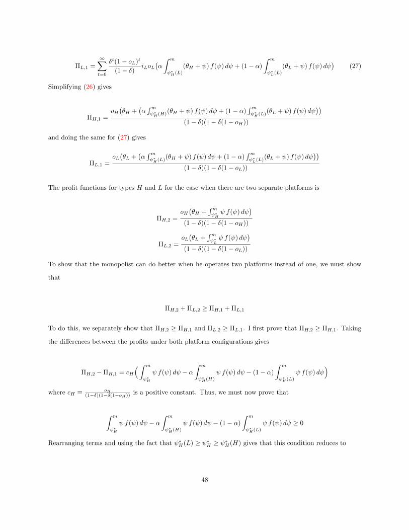
ΠL,1 =

∞∑t=0

δt(1− oL)t

(1− δ)iLoL

(α

∫ m

ψ∗H(L)

(θH + ψ) f(ψ) dψ + (1− α)

∫ m

ψ∗L(L)

(θL + ψ) f(ψ) dψ)

(27)

Simplifying (26) gives

ΠH,1 =oH(θH +

(α∫mψ∗H(H)

(θH + ψ) f(ψ) dψ + (1− α)∫mψ∗H(L)

(θL + ψ) f(ψ) dψ))

(1− δ)(1− δ(1− oH))

and doing the same for (27) gives

ΠL,1 =oL(θL +

(α∫mψ∗H(L)

(θH + ψ) f(ψ) dψ + (1− α)∫mψ∗L(L)

(θL + ψ) f(ψ) dψ))

(1− δ)(1− δ(1− oL))

The profit functions for types H and L for the case when there are two separate platforms is

ΠH,2 =oH(θH +

∫mψ∗H

ψ f(ψ) dψ)

(1− δ)(1− δ(1− oH))

ΠL,2 =oL(θL +

∫mψ∗Lψ f(ψ) dψ

)(1− δ)(1− δ(1− oL))

To show that the monopolist can do better when he operates two platforms instead of one, we must show

that

ΠH,2 + ΠL,2 ≥ ΠH,1 + ΠL,1

To do this, we separately show that ΠH,2 ≥ ΠH,1 and ΠL,2 ≥ ΠL,1. I first prove that ΠH,2 ≥ ΠH,1. Taking

the differences between the profits under both platform configurations gives

ΠH,2 −ΠH,1 = cH

(∫ m

ψ∗H

ψ f(ψ) dψ − α∫ m

ψ∗H(H)

ψ f(ψ) dψ − (1− α)

∫ m

ψ∗H(L)

ψ f(ψ) dψ)

where cH ≡ oH(1−δ)(1−δ(1−oH)) is a positive constant. Thus, we must now prove that

∫ m

ψ∗H

ψ f(ψ) dψ − α∫ m

ψ∗H(H)

ψ f(ψ) dψ − (1− α)

∫ m

ψ∗H(L)

ψ f(ψ) dψ ≥ 0

Rearranging terms and using the fact that ψ∗H(L) ≥ ψ∗H ≥ ψ∗H(H) gives that this condition reduces to

48

1

α

∫ ψ∗H(L)

ψ∗H

ψ f(ψ) dψ − 1

1− α

∫ ψ∗H

ψ∗H(H)

ψ f(ψ) dψ ≥ 0

Note now that the thresholds ψ∗H(H) and ψ∗H(L) are both functions of α. When ψ∗H(L) = ψ∗H(H), the

condition is automatically satisfied since both integrals will be 0. Now we want to show that as the gap

between the two thresholds ψ∗H(H) and ψ∗H(L) increases, the condition still holds. To do this, for any value

of α, fix ψ∗H(H). By showing that the derivative of the right-hand side of the condition is increasing in

ψ∗H(L), we will have shown that the condition holds.

Rewriting the condition by holding ψ∗H(H) constant and varying ψ∗H as functions of ψ∗H(L) gives me

1

α

∫ ψ∗H(L)

ψ∗H(ψ∗H(L))

ψ f(ψ) dψ − 1

1− α

∫ ψ∗H(ψ∗H(L))

ψ∗H(H)

ψ f(ψ) dψ ≥ 0

Taking the derivative of the left-hand side of the condition with respect to ψ∗H(L) by using the Leibniz Rule

gives

∂LHS

∂ψ∗H(L)=

1

α

(∫ ψ∗H(L)

ψ∗H(ψ∗H(L))

0 dψ + ψ∗H(L) f(ψ∗H(L))× 1− ψ∗H f(ψ∗H)∂ψ∗H(ψ∗H(L))

∂ψ∗H(L)

)

− 1

1− α

(∫ ψ∗H(ψ∗H(L))

ψ∗H(H)

0 dψ + ψ∗H f(ψ∗H)∂ψ∗H(ψ∗H(L))

∂ψ∗H(L)− ψ∗H(H) f(ψ∗H(H))× 0

)Recall that

1− F (ψ∗H) = α(1− F (ψ∗H(H))) + (1− α)(1− F (ψ∗H(L)))

=⇒ F (ψ∗H) = αF (ψ∗H(H)) + (1− α)F (ψ∗H(L))

=⇒ ψ∗H = F−1(αF (ψ∗H(H)) + (1− α)F (ψ∗H(L)))

=⇒ ∂ψ∗H(ψ∗H(L))∂ψ∗H(L) =

(1−α)F′(ψ∗H(L))

F ′ (ψ∗H)

=⇒ ∂ψ∗H(ψ∗H(L))∂ψ∗H(L) =

(1−α)f(ψ∗H(L))f(ψ∗H)

Substituting this into the earlier condition and simplifying gives

∂LHS

∂ψ∗H(L)=

1

αψ∗H(L) f(ψ∗H(L))− 1

αψ∗H f(ψ∗H)

(1− α)f(ψ∗H(L))

f(ψ∗H)− 1

(1− α)ψ∗H f(ψ∗H)

(1− α)f(ψ∗H(L))

f(ψ∗H)

49

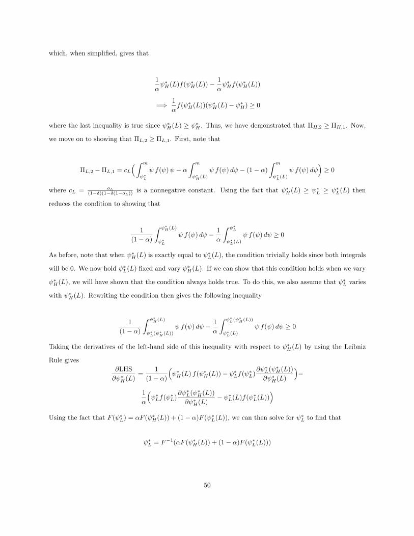
which, when simplified, gives that

1

αψ∗H(L)f(ψ∗H(L))− 1

αψ∗Hf(ψ∗H(L))

=⇒ 1

αf(ψ∗H(L))(ψ∗H(L)− ψ∗H) ≥ 0

where the last inequality is true since ψ∗H(L) ≥ ψ∗H . Thus, we have demonstrated that ΠH,2 ≥ ΠH,1. Now,

we move on to showing that ΠL,2 ≥ ΠL,1. First, note that

ΠL,2 −ΠL,1 = cL

(∫ m

ψ∗L

ψ f(ψ)ψ − α∫ m

ψ∗H(L)

ψ f(ψ) dψ − (1− α)

∫ m

ψ∗L(L)

ψ f(ψ) dψ)≥ 0

where cL = oL(1−δ)(1−δ(1−oL)) is a nonnegative constant. Using the fact that ψ∗H(L) ≥ ψ∗L ≥ ψ∗L(L) then

reduces the condition to showing that

1

(1− α)

∫ ψ∗H(L)

ψ∗L

ψ f(ψ) dψ − 1

α

∫ ψ∗L

ψ∗L(L)

ψ f(ψ) dψ ≥ 0

As before, note that when ψ∗H(L) is exactly equal to ψ∗L(L), the condition trivially holds since both integrals

will be 0. We now hold ψ∗L(L) fixed and vary ψ∗H(L). If we can show that this condition holds when we vary

ψ∗H(L), we will have shown that the condition always holds true. To do this, we also assume that ψ∗L varies

with ψ∗H(L). Rewriting the condition then gives the following inequality

1

(1− α)

∫ ψ∗H(L)

ψ∗L(ψ∗H(L))

ψ f(ψ) dψ − 1

α

∫ ψ∗L(ψ∗H(L))

ψ∗L(L)

ψ f(ψ) dψ ≥ 0

Taking the derivatives of the left-hand side of this inequality with respect to ψ∗H(L) by using the Leibniz

Rule gives

∂LHS

∂ψ∗H(L)=

1

(1− α)

(ψ∗H(L) f(ψ∗H(L))− ψ∗Lf(ψ∗L)

∂ψ∗L(ψ∗H(L))

∂ψ∗H(L)

)−

1

α

(ψ∗Lf(ψ∗L)

∂ψ∗L(ψ∗H(L))

∂ψ∗H(L)− ψ∗L(L)f(ψ∗L(L))

)Using the fact that F (ψ∗L) = αF (ψ∗H(L)) + (1− α)F (ψ∗L(L)), we can then solve for ψ∗L to find that

ψ∗L = F−1(αF (ψ∗H(L)) + (1− α)F (ψ∗L(L)))

50

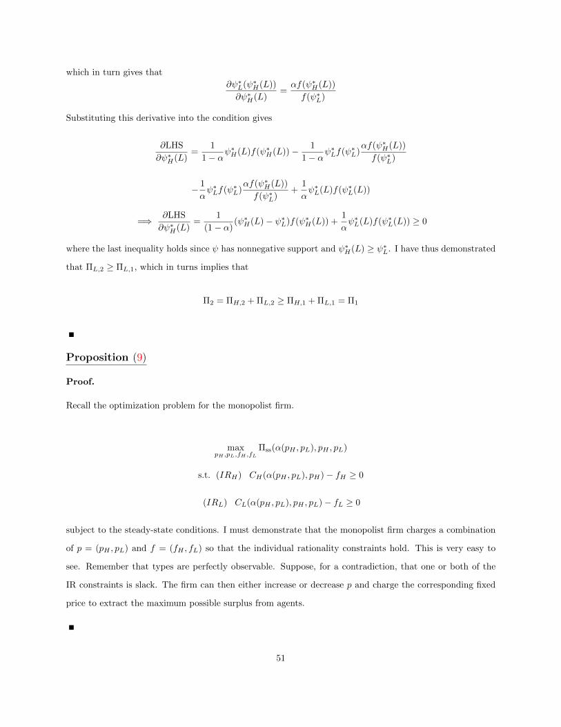
which in turn gives that

∂ψ∗L(ψ∗H(L))

∂ψ∗H(L)=αf(ψ∗H(L))

f(ψ∗L)

Substituting this derivative into the condition gives

∂LHS

∂ψ∗H(L)=

1

1− αψ∗H(L)f(ψ∗H(L))− 1

1− αψ∗Lf(ψ∗L)

αf(ψ∗H(L))

f(ψ∗L)

− 1

αψ∗Lf(ψ∗L)

αf(ψ∗H(L))

f(ψ∗L)+

1

αψ∗L(L)f(ψ∗L(L))

=⇒ ∂LHS

∂ψ∗H(L)=

1

(1− α)(ψ∗H(L)− ψ∗L)f(ψ∗H(L)) +

1

αψ∗L(L)f(ψ∗L(L)) ≥ 0

where the last inequality holds since ψ has nonnegative support and ψ∗H(L) ≥ ψ∗L. I have thus demonstrated

that ΠL,2 ≥ ΠL,1, which in turns implies that

Π2 = ΠH,2 + ΠL,2 ≥ ΠH,1 + ΠL,1 = Π1

Proposition (9)

Proof.

Recall the optimization problem for the monopolist firm.

maxpH ,pL,fH ,fL

Πss(α(pH , pL), pH , pL)

s.t. (IRH) CH(α(pH , pL), pH)− fH ≥ 0

(IRL) CL(α(pH , pL), pH , pL)− fL ≥ 0

subject to the steady-state conditions. I must demonstrate that the monopolist firm charges a combination

of p = (pH , pL) and f = (fH , fL) so that the individual rationality constraints hold. This is very easy to

see. Remember that types are perfectly observable. Suppose, for a contradiction, that one or both of the

IR constraints is slack. The firm can then either increase or decrease p and charge the corresponding fixed

price to extract the maximum possible surplus from agents.

51

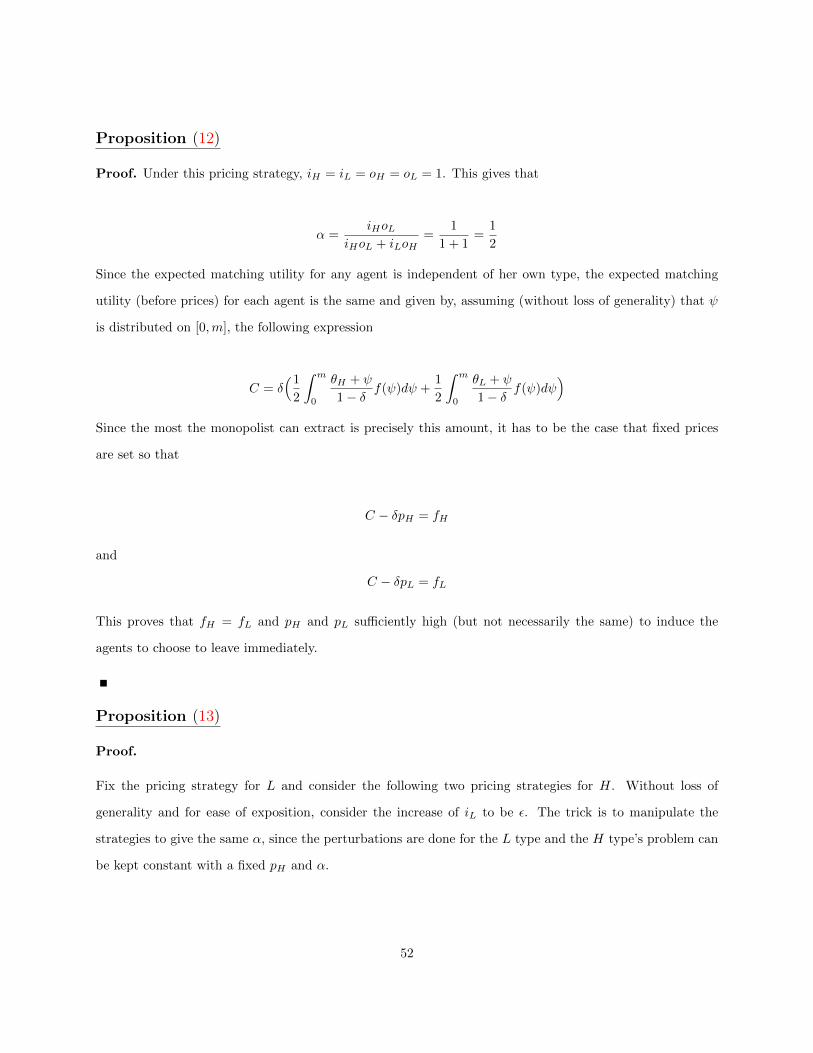
Proposition (12)

Proof. Under this pricing strategy, iH = iL = oH = oL = 1. This gives that

α =iHoL

iHoL + iLoH=

1

1 + 1=

1

2

Since the expected matching utility for any agent is independent of her own type, the expected matching

utility (before prices) for each agent is the same and given by, assuming (without loss of generality) that ψ

is distributed on [0,m], the following expression

C = δ(1

2

∫ m

0

θH + ψ

1− δf(ψ)dψ +

1

2

∫ m

0

θL + ψ

1− δf(ψ)dψ

)Since the most the monopolist can extract is precisely this amount, it has to be the case that fixed prices

are set so that

C − δpH = fH

and

C − δpL = fL

This proves that fH = fL and pH and pL sufficiently high (but not necessarily the same) to induce the

agents to choose to leave immediately.

Proposition (13)

Proof.

Fix the pricing strategy for L and consider the following two pricing strategies for H. Without loss of

generality and for ease of exposition, consider the increase of iL to be ε. The trick is to manipulate the

strategies to give the same α, since the perturbations are done for the L type and the H type’s problem can

be kept constant with a fixed pH and α.

52

Strategy 1 (old) : iL,old = 1− ε and pL,old

Strategy 2 (new) : iL,new = 1 and pL,new > pL,old

Why these two strategies? Well, look at the expression of α given by

α(pH , pL) =

iHoH(pH)

iHoH(pH) + iL

oL(pH ,pL)

=

iHoH(pH)

iHoL(pH ,pL)+iLoH(pH)oH(pH)oL(pH ,pL)

=iHoL(pH , pL)

iHoL(pH , pL) + iLoH(pH)

Increasing iL from the old to new strategy decreases α. To keep α constant, the firm can then manipulate

pL to increase oL. Since oL partly depends on L’s threshold, and the threshold strictly decreases with prices,

the firm can increase pL in order to decrease L’s threshold (effectively making L less picky), forcing Ls to

exit the platform faster. This explains why pL,new > pL,old. So then the question is: what outflow rates or

probability of matching for L will keep α constant?

Define

oL,i ≡ Probability that L matches under strategy i

di ≡ Number of dates that L goes on before matching under strategy i.

Computing the expected number of dates that L goes under both pricing strategies gives

E(d1) =

∞∑t=1

oL,1 (1− oL,1)t−1 t =1

oL,1

E(d2) =1

oL,2

Keeping the mass of L agents on the platform equal under both strategies gives

µL,1 ≡1− εoL,1

=1

oL,2≡ µL,2 =⇒ oL,2 =

oL,11− ε

Now, recall that ψ is drawn from the interval [0,m]. Feasible utility ranges for L are then [θL, θL +m] when

matching with L and [θH , θH + m] when matching with H. Let φ∗t ≡ L’s utility threshold when matching

with type t. Then the probabilities of acceptance are:

P (L accepts L) = P (φL ≥ φ∗L) =θL +m− φ∗L

m

53

P (H accepts L) = P (φH ≥ φ∗H) =θH +m− φ∗H

m

Fixing the pricing strategy for H types implies that H’s decision is fixed, which means φ∗H is fixed. Define

the expected utility for L of matching in any period under strategy i is defined as

UL(φ∗H , φ∗L,i) =

1

2(α(φ∗H + θH +m) + (1− α)(φ∗L + θL +m))

and the outflow rate for L types under pricing strategy i is defined as

oL,i(φ∗H , φ

∗L,i) =

1

m(α(m+ θH − φ∗H) + (1− α)(m+ θL − φ∗L,i)

Note that going from pricing strategy 1 to 2 requires that φ∗L changes. To find the changed threshold utility

value, solve

oL,2 =oL,11− ε

=⇒ φ∗L,2 =φ∗L,1 − αφ∗L,1 − ε(m+ θL + α(θH − θL)− αφ∗H)

(1− ε)(1− α)

We can write out expected lifetime utilities:

EU2 =

∞∑t=1

δt−1oL,11− ε

(1− oL,11− ε

)t−1UL(φ∗H , φ∗L,2)

EU1 =

∞∑t=1

δt−1oL,1(1− oL,1)t−1UL(φ∗H , φ∗L,1)

Now, I would like to algebraically show that

limε→0

EU2 − (1− ε)EU1

ε> 0

This establishes the result that profit for the monopolist is strictly higher under pricing strategy 2 than 1,

since the profit that the monopolist can extract from each agent is precisely the expected lifetime utility of

the agent, and so the aggregrate profit that the monopolist extracts is iL times the expected lifetime utility.

Algebraically,

limε→0

EU2 − (1− ε)EU1

ε=

a

2(m+ δ(α(θH + ε∗H(L)) + (1− α)(θL + ε∗L(L))))2> 0

54

Corollary (8)

Proof.

This corollary follows from the previous proposition. Note that the condition on the proposition that

ψ∗L(L) ∈ (0,m) is a ‘global’ condition which is assumed to hold for all pL.

55

References

Armstrong, M. (2006). Competition in Two-Sided Markets. RAND Journal of Economics 37(3), 668-691.

Adachi, H. (2003). A Search Model of Two-Sided Matching under Nontransferable Utility. Journal of Eco-

nomic Theory 113(2), 182-198.

Abdulkadiroglu, A., P. Pathak, and A. Roth. (2005). The New York City High School Match. American

Economic Review Papers and Proceedings (May 95), 364-367.

Abdulkadiroglu, A., P. Pathak, A. Roth, and T. Sonmez. (2005). The Boston Public School Match. American

Economic Review Papers and Proceedings (May 95), 368-371.

Azevedo, E. and J. Leshno. (2012). A Supply and Demand Framework for Two-Sided Matching Markets.

Working Paper.

Becker, G. S. (1973). A Theory of Marriage: Part 1. Journal of Political Economy 81(4), 813-846.

Bester, H. (1994). Price Commitment in Search Markets. Journal of Economic Behavior and Organization

25(1), 109-120.

Bloch, F. and H. Ryder. (2000). Two-Sided Search, Marriages, and Matchmakers. International Economic

Review 41(1), 93-115.

Browning, M., P. Chiappori, and Y. Weiss. (2014). Economics of the Family. Cambridge Surveys of Economic

Literature: Cambridge University Press.

Bulow, J. and J. Levin. (2006). Matching and Price Competition. American Economic Review, 96(3), 652-

668.

Burdett, K. (1978). A Theory of Employee Job Search and Quit Rates. American Economic Review, 68(1),

212-220.

Burdett, K. and M. Coles. (1997). Marriage and Class. Quarterly Journal of Economics 112, 141-168.

Burdett, K. and R. Wright. (1998). Two-sided Search with Nontransferable Utility. Review oF Economic

Dynamics 1(1), 220-245.

Cabral, L. (2011). Dynamic Price Competition with Network Effects. Review of Economic Studies 78, 83-111.

Cornelius, T. (2003). A Search Model of Marriage and Divorce. Review of Economic Dynamics 6(1), 135-155.

56

Damiano, E. and L. Hao. (2007). Price Discrimination and Efficient Matching. Economic Theory 30, 243-263.

Flanders, S. (2014). Mirror Matches: Analyzing Matching Markets with N-Dimensional Preferences. Working

Paper.

Gale, D. and L.S. Shapley. (1962). College Admissions and the Stability of Marriage. The American Mathe-

matical Monthly 69(1), 9-15.

Hagiu, A. (2006). Pricing and Commitment by Two-Sided Platforms. RAND Journal of Economics 37(3),

720-737.

Halaburda, H. and M. Piskorski. (2011). Competing by Restricting Choice: The Case of Search Platforms.

Harvard Business School Working Paper 10-098.

Hoppe, H., B. Moldavanu, and A. Sela. (2011). The Theory of Assortative Matching Based on Costly Signals.

Economic Theory 47, 75-104.

Hotelling, H. (1929). Stability in Competition. The Economic Journal 39(153), 41-57.

Kojima, F. and P. Pathak. (2009). Incentives and Stability in Large Two-Sided Matching Markets. American

Economic Review 99(3), 608-627.

McCall, J. (1970). Economics of Information and Job Search. The Quarterly Journal of Economics 84(1),

113-126.

Mortensen, D. and C. Pissarides. (1994). Job Creation and Job Destruction in the Theory of Unemployment.

Review of Economic Studies 61, 397-415.

Rochet, J. and J. Tirole. (2006). Two-Sided Markets: A Progress Report. RAND Journal of Economics

37(3), 645-667.

Rochet, J. and J. Tirole. (2010). Platform Competition in Two-Sided Markets. Journal of the European

Economic Association 1(4), 990-2019.

Rogerson, R., R. Shimer, and R. Wright. (2005). Search-Theoretic Models of the Labor Market: A Survey.

Journal of Economic Literature Vol XLIII, 959-988.

Roth, A., T. Sonmez, and M.U. Unver. (2005). Pairwise Kidney Exchange. Journal of Economic Theory 125,

151-188.

57

Roth, A., T. Sonmez, and M.U. Unver. (2007). Efficient Kidney Exchange: Coincidence of Wants in Markets

with Compatibility-Based Preferences. The American Economic Review 97(3), 828-851.

Rysman, M. (2009). The Economics of Two-Sided Markets. Journal of Economic Perspectives 23(3), 125-143.

Salop, S. C. (1979). Monopolistic Competition with Outside Goods. The Bell Journal of Economics 10(1),

141-156.

Shapley, L.S. and M. Shubik. (1971). The Assignment Game I: The Core. International Journal of Game

Theory 1(1), 111-130.

Shimer, R. and L. Smith. (2001). Matching, Search, and Heterogeneity. Advances in Macroeconomics 1(1).

Weyl, G. (2010). A Price Theory of Multi-Sided Platforms. American Economic Review 100(4), 1642-1672.

58