extractive industries, production shocks and criminality...

Extractive Industries, Production Shocks andCriminality: Evidence from a Middle-Income Country∗

Sebastian Axbard† Jonas Poulsen‡ Anja Tolonen§

January 13, 2015Preliminary and Incomplete

Abstract

Extractive industries are key to development in many countries, accounting for large sharesof government revenue and GDP. However, there is a vast and growing literature that links ex-tractive industries to conflicts and war in countries with weak institutions. We are, to ourknowledge, the first to investigate whether extractive industries can cause economic and vio-lent crime. We focus on South Africa, a country with a significant mining industry and highlevels of criminality. We exploit time and geographic variation, in addition to fluctuationsin international mineral prices, in a fixed effects and an instrumental variables approach. Incontrast to earlier findings on other forms of social conflict, we find that areas endowed withhigher levels of natural resources show no increase in crime when a mine opens. However, theclosure of a mine leads to a large and significant increase in both property and violent crime.Subsequently, we show that the migration flows and income opportunities created by the min-ing industry are two important channels through which mining affect criminality.Keywords: Extractive Industries, Mining, Crime, Violence, EmploymentJEL classification: K42, D74, O13

∗We thank seminar participants at UCLS Uppsala University as well as Niklas Bengtsson, Amir Jina, MikaelLindahl, June Luna, Edward Miguel, Andreea Mitrut, Eva Mork, Imran Rasul and Mans Soderbom for valuablecomments. We are also grateful to Statistics South Africa as well as the Institute for Security Studies for providingdata.

†Uppsala University, [email protected]‡Uppsala University, [email protected]§University of Gothenburg, [email protected]

1

1 Introduction

Extractive industries are key to economic development in many countries. Mineral resources, inparticular, play a dominant role in 81 countries that collectively account nearly 70% of those in ex-treme poverty (World Bank, 2014). Many have discussed this association in terms of the resourcecurse (see van der Ploeg, 2011 for an overview), but fewer have looked at the extractive industry asan inherent feature of many developing economies which presents both potential harms and poten-tial benefits. In developing countries, mining is economically important, and approximately 1% ofthe global labor force works in mining (ILO, 2010). Mining has been found to spur local structuralchange, benefitting local labor markets (Aragon and Rud, 2013; Kotsadam and Tolonen, 2013),and the industry has been crucial for countries such as Botswana and Namibia in the transitionfrom poor to middle income.

However, there is a large and growing literature that link extractive industries to conflict andcivil war in contexts with weak institutions.1 The main mechanism emphasized in this literatureis that a shock to an extractive industry might alter the incentives for appropriation (see e.g. DalBo and Dal Bo, 2011) since the increase in potential rents can drive social conflict. How thisextends to criminality is not clear, and to our knowledge never previously empirically tested. Weposit an additional hypothesis, namely that an increase in extractive activities that generate jobopportunities which affect the opportunity cost of crime, as outlined by Becker (1968).

In this paper, we focus on South Africa, a middle-income country with relatively stable politicalinstitutions where social conflict mainly comprises violent and economic crime, rather than largerscale protest or civil conflicts. In such a setting the income opportunity channel could potentiallyplay a more dominant role, than that of rent seeking behavior. Hence, in this setting it is difficult topredict the effect of mining on criminality a priori. Nonetheless, we argue that this is an importantsetting to study since there are a large number of countries with similar institutional settings aswell as high natural-resource endowments, such as Botswana, Brazil, Mexico and Romania.

Additionally, we have particular interest in understanding dynamics of crime in South Africa.Crime, and violent crime in particular, is a serious threat to development in the country. For ex-ample, our data show that 13,123 men, 2,266 women and 827 children were murdered in 2012/13,making it one of the most murder dense regions of the world. Violent crime is a major factor be-hind the emigration of skilled labor, gated communities and a flourishing private security sector.2

At the same time, South Africa has the fifth largest mining industry in the world which contributesto around 8% of GDP and created 1.3 million jobs in 2012 (Chamber of Mines, 2014). Recently,

1Collier and Hoeffler (1998, 2004 & 2005) were pioneers of the literature examining linkages between naturalresources civil war. Recent work include Berman, Couttenier, Rohner & Thoenig (2014), Buonanno et al. (2013) &Maystadt et al. (2014).

2Citation needed

1

media, as well as government, attention has been directed towards the link between mining andviolence, not least since the 2012 Marikana massacre where 44 miners were killed. A New YorkTimes report (NYT, 2013) suggests that violent crime has risen as townships have ”fallen on hardtimes as gold mines have closed”. In this paper, we examine the causal effect of mining activityon crime between 2003 and 2012 using several different estimation strategies. Specifically, weexplore the effect on crime rates at different spatial scales from mining activity and productionshocks, what types of crimes that are affected, and lastly we try to disentangle the mechanismsbehind our findings.

One concern is that mine production is affected by crime levels in the proximity of a mine. Toovercome this potential reverse-causation, we employ an instrumental variable approach where weinstrument the number of actively-producing mines of a specific mineral in a given location by theinternational price of that mineral. Other papers (c.f. Allcott and Keniston, 2014; Berman et al.,2014; Tolonen, 2015) have used international prices as exogenous variation in mining production,but we instrument mining activity with prices rather than rely on the reduced-form relationship (asdo von der Goltz and Barnwal, 2014). The first stage coefficient is positive and highly statisticallysignificant: the higher the international price of a given mineral, the larger the number of minesactively producing such minerals. In the second-stage analysis, we investigate how a change inmining activity affects the crime rate in police precincts.3 We find a negative and significanteffect of mining production on both economic and violent crime. In particular, as mining activityincreases, induced by a higher international mineral price, crime rates fall by approximately 7%for each additional mine. This negative association is further supported by the results from a fixed-effects estimation of the relationship between the number of active mines in a police precinct onlocal crime rates. To capture effects at a higher aggregate level we replicate the results at the largermunicipality level and find similar effects.

Subsequently, we investigate the dynamic effects of production shocks. We allow for assy-metric effects of mine openings and mine closings. We find that when a mine stops actively pro-ducing, crime rates increase substantially. This finding argues for the opportunity-cost channel:when a mine closes, direct and indirect employment decreases locally, income decreases, and theincentives to commit a crime increase. Similarly, we find suggestive evidence that as a mine startsproducing, crime rates fall.

Poor availability of mine employment numbers and labor market information at a sufficientlydisaggregated geographic level makes it hard to further asses the viability of the income channel.However, following recent economic literature (Bleakley and Lin, 2012; Henderson et al., 2012;Michalopoulos and Papaioannou, 2013; Lowe, 2014; Storeygard, 2012; Pinkovskiy, 2013), weproxy economic activity in police precincts using satellite data on lights at night. Doing so, we

3Police precincts are South African administrative areas, in general smaller than municipalities.

2

find that the number of active mines has a positive effect on light density. However, when a minecloses, local economic activity falls. These findings support the hypothesis that the causal effectof mine closure on crime goes through an income channel. Furthermore, following the theoryoutlined by Dal Bo and Dal Bo (2011), we show that our results seem to be driven by mining thatis relatively more labor intensive, a finding that also speaks for the income channel.

In addition, we consider to what extent labor migration to mining areas can be a mechanismthrough which crime rates are affected. Prior to democratization, the labor in South African mineswas supplied by domestic and international migrants, enforced by Apartheid policy. However, la-bor migration remains important in the mining sector until today.4 There are two main reasons whywe believe migration to be important. First, the migrant-labor system5 is associated with serioussocial concerns, such as single-sex hostels and informal settlements, characterised by lack of socialservices, high crime rates and unemployment (Aliber, 2003; Hamann and Kapelus, 2004). Second,the size of the mine induced migration flow will determine if the employment rate increases ordecreases, and determine the local wage rate.

We establish that the number of active mines in a municipality increase the share of migrants inthe population with 23% for each additional mine. In fact, when a mine starts producing (a positiveshock in mining activity) migration increases by 18%. Thereafter, we compare the effect of miningactivity on crime in municipalities with high and low average migration rates. Results from thisanalysis are imprecisely estimated but provide suggestive evidence for migration patterns playinga role in which mining activity affect crime. We find that production starts in low-migration areasare associated with lower crime rates and typically small and insignificant effects on crime when amine stops producing. However, in high migration areas both production starts and stops are asso-ciated with higher crime rates. We see two potential explanations: first, because inward migrationincreases competition over jobs, second that production shocks in high migration areas affect indi-viduals with weaker ties to the local labor market, hence the income opportunities provided by themine is more important for this group.

Previous literature on extractive industries and social conflict find detrimental effects. Like-wise, looking at the effect of mining activity on public violence (the outcome most closely relatedto what has been used in related studies), we display suggestive evidence that earlier findings alsoapply to South Africa. However, we show that extractive industries can change a specific type ofsocial conflict: criminality. Mining activity seems to lower crime rates although a stop in produc-

4In 1997, a few years after the advent of democracy, 95% of all mine workers were still migrants, most from ruralSouth Africa, Lesotho and Mozambique.

5The system has even been called a ”scar on the face of democratic South Africa” by Deputy President Motlanthe(Financial Times, April 2014). Policies have aimed at improving the social situation and single-sex hostels have be-come less common. However, oftentimes the hostels have been replaced by informal settlements where mine workerslive.

3

tion increases crime rates. Presumably, the effect is going through income opportunities stemmingfrom mining activity. Whereas in a weak institutional setting, mining opportunities can increasethe risk of conflict by providing funding for criminal gangs or rebel groups, we show that in amiddle-income setting with better institutions, the mineral base can lead to more social stability,as indicated by lower crime rates.

The next section looks at previous literature on extractive industries and violence. Section 3gives a background on the mining industry and crime in South Africa. Section 4 describes the dataused in the estimations and Section 5 goes through the empirical strategies. The results from ourmain specifications, mechanism checks and tests of robustness are given in Section 6. Section 7concludes the paper.

2 Previous Literature

In this paper, we use production changes in mineral and coal mines to identify the effects of miningactivity on crime. It is, to our knowledge, the first paper to investigate the effect of extractiveindustries on various types of crime, and using official records from the police. We add to theliterature on the ”resource curse”, focusing on the link between natural resource extraction andsocial conflict (for an overview of the resource curse, see van der Ploeg 2011).

There is a growing empirical literature on the effects of extractive industries and violence. Re-cent papers have explored the links between extractive industries and violence at a sub-nationallevel (see for example Caselli et al. 2013; Maystadt et al., 2013; Rohner 2006). Couttenier et al.,(2014) find that minerals play a role historically and presently for homicide rates in the US; andBuonanno et al., (2013) find a relationship between natural resource endowments and the emer-gence of the Sicilian mafia. Bellows and Miguel (2009) show that diamond mining increased armedclashes during the civil war in Sierra Leone. Aragon and Rud (2013), however, find that householdmembers in mining communities in Peru are no more likely to report having been affected by acriminal act than surveyed households further away.

The paper most similar in spirit to ours is Berman et al., (2014) who explore the impact ofmining on conflict for all African countries between 1997 and 2010. The authors exploit within-mining area panel variation in violence due to changes in the world price of the relevant mineral andfind that mining activity increases local area conflict, as collected by the ACLED dataset. Similarly,we explore the effect of changes in mining activity induced by changes in mineral prices, but focuson South African crime rates. We investigate whether the patterns of detrimental effects stemmingfrom extractive industries described above also is true for a middle-income country, using officialpolice records for economic and violent crime, rather than multi-origin data sets on conflict. Thus,apart from public violence which we have data on, we test the predictions from the literature on

4

extractive industries and conflict for idiosyncratic violent crimes such as murder and assault, andproperty crime such as burglary. An additional contribution of this paper is that we can instrumentmining production with international prices, while Berman et al., (2014) look at the reduced-formrelationship between prices and conflict.

A first stepping stone for understanding the aforementioned research question and earlier em-pirical work is Dal Bo and Dal Bo (2011), providing a theoretical investigation of how economicshocks and policies affect the intensity of conflict and crime. In particular, the authors show howpositive productivity shocks to labor-intensive industries in less-developed countries (e.g. agricul-ture in Sub-Saharan Africa) diminish conflict, while positive shocks to capital-intensive industries(e.g. the oil industry) increase it. The intuition is that a positive shock to a capital-intensive indus-try will cause it to expand while the labor-intensive industry contracts, which make labor relativelymore abundant resulting in lower wages. Since wages decrease relative the value of appropriableresources, appropriation will increase. That is, the incentives for social conflict will increase. Thisintuition is for example supported by Dube and Vargas (2013) who find that conflict in Colombiaincreased following a fall in coffee prices, which might be considered a labor-intensive product,and an increase in oil prices, which might be considered a capital-intensive product. Similarly, wetest this channel by splitting mining into open-pit (more capital intensive) and underground (morelabor intensive).6

Another stepping stone in understanding the link between mining and crime is the theory ofthe economics of crime developed in Becker (1968). The intuition is similar to that of Dal Bo andDal Bo (2011). Crime is a type of job chosen in competition with regular wage work and in thiscase, an increase in mining activity leads to an increase in the opportunity cost of crime if certainrequirements are fulfilled.7 In other words, the closure of a mine or lower production will leadto lower incomes among mine workers and societies that are dependent on the mine. The drivingforces behind burglary, robbery and car hijackings, for example, should then become stronger.

6The mining industry in South Africa employs around half a million people directly, and many more indirectly(Chamber of Mines, 2014). The relatively high number of direct employment is foremost due to the depths of SouthAfrican mines that makes mechanization less common. The South African mining industry is therefore relatively morelabour intensive compared to other mining countries, including its African neighbors.

7Specifically that mining increases the supply of jobs, and/or market clearing wage. If inward migration exceedsthe new jobs created, total employment or market wages need not increase. Furthermore, in the case of a mine leadingto local Dutch Disease effects and crowd out other industries, such as manufacturing, these two relationships need nothold.

5

3 Background

3.1 Crime in South Africa

Although South Africa has seen a huge increase in the number of private security guards as well asa tripling of government spending on crime prevention since the mid-1990’s, the country is one ofthe most crime stricken in the world. The Economist (2010) notes that ”a staggering 50 murders,100 rapes, 330 armed robberies and 550 violent assaults are recorded every day”. Recorded crimelevels increased during the last decade of apartheid rule and peaked in the early 1990’s. The hopethat these levels would decrease after 1994 was not met. Rather, in the period between 1994 and2000, crime increased. For example, the annual increase in the number of crimes was higherin 1999 than all previous years after 1994. These changes were mainly driven by huge rises incommon robbery (121%), residential burglary (25%), assault (22%), rape (21%) and car hijacking(20%). In general, violent crime stands out as the one category where South Africa saw a consistentincrease from 1994. The country was considered having the highest per capita rates of murder andrape and the second highest rate of robbery and violent theft (Louw and Schonteich 2001). Itshould however be noted that South African crime follows a geographic pattern. Burglaries, forexample, are more common in police precincts (police station jurisdictions) that are wealthier thanneighboring precincts, pointing toward migratory criminality behavior (Demombynes and Ozler2005)

Poverty, unemployment and labor migration are common South African experiences: chronicpoverty exists (Aliber 2003), and unemployment is high. In 2004, the beginning of our study pe-riod, unemployment was 41% (broad definition) or 30% (narrow definition) (Kingdon and Knight2004). In 2012 the unemployment rate had decreased somewhat, to an average of 25.2%. There isthus a lack of income opportunities for many South Africans, which can be a partial explanationfor the high crime rates.

3.2 The Mining Industry

Large-scale mining is a notable element in South Africa’s history. It first started in 1867 whenalluvial diamonds were found along the Orange River, soon followed by the Kimberley diamonddiscovery and the Witwatersrand Gold Rush in the 1880’s. The gold rush led to the onset of TheMineral Revolution: the rapid mineral-driven economic growth that laid the foundations for SouthAfrica’s economic capital Johannesburg. Today the South African mining industry is the fifthlargest in size globally (Chamber of Mines 2012), and the country may have what is the largestmineral endowment despite a long history of extraction (Carrol 2012). South Africa is a producerof many different metals and minerals, and the economically most important mineral groups are

6

platinum (platinum group metals, PGMs), gold, coal and iron ore.8 The country is the biggestglobal producer of PGMs and gold, as well as manganese and chromium, although the latter twoare smaller shares of the South African economy (Antin 2013).

525,000 people were employed in mining in 2012, increasing from 436,000 in 2003 (Chamberof Mines, 2013). Only roughly 15% of the miner workforce in 2013 was women (StatsSA 2013).The employment opportunities are concentrated to certain regions, such as the North West (141thousand miners in 2012), Mpumalanga (79 thousand), Limpopo (73 thousand), and Gauteng (32thousand) but also Free State, KwaZulu-Natal, Northern Cape has significant mining employment(StatsSA, 2013).

Despite generating many employment opportunities, the sector’s economic importance relativeGDP exceeds its importance in terms of employment. In 2011, the sector employed 0.7% of theworkforce, but made up 8.8% of national GDP. However, while in the latter years the sector hascontributed to on average 8% of GDP, it constitutes as much as 18% of all economic activity, ifupstream and downstream industries are included.

Despite the small share of employment to value created, labor constitute a significant share ofthe production costs, making up roughly 40%. That however masks heterogeneity: for deep-levelmines it can be over 60%, and open cast mines about 30%, a fact that we make use of in thesubsequent analysis. The wage burden has increased over time. From 2007 to 2012, negotiatedwage increases have been above inflation rates, putting more pressure on the industry and leadingto staff reductions (Antin 2013; PWC 2011).

3.3 South African history of mining, migration and criminality

Recently, media has focused on uprisings in South African mining communities. A demonstrationfor wage increases in the Marikana Platinum mine in 2012 led to violent clashes and the death of34 workers. The incident was one of the most violent in the democratic South Africa. NGO’s havepointed to the clash as a result of the widespread poverty and grievances among the migrant mineworkers (Human Rights Watch 2013). Such a narrative of grievances is far from new within theSouth African mining industry. The history of mining dates long back and so does its history ofviolence and criminality. In fact, to some extent they may be interconnected.

The gold deposits in present-day Johannesburg were the destinations of fortune seekers fromEurope and other parts of the African continent. The migration movement was sudden and strong:from a mining camp worthy of 3,000 individuals in 1887, Johannesburg grew to a city of 100,000 inonly 22 years. Migrant gangs formed in the mining communities during the early 20th century, anddefined what was to be the criminal landscape of Johannesburg (Kynoch 2005). Social exclusion of

8These are the largest mineral groups in terms of employment and sales.

7

migrants is thought to be part of the reason why migrants on the fringe of the mining communitiesturned to criminality: migrant workers were the lowest on the hierarchical social ladder, confinedto the roughest and most menial employments (Kynoch 1999). Moreover, the migrant workersemployed in the mine were kept aside from the rest of the urban South Africa, as part of Britishcolonial policy (Antin 2013), and later part of apartheid policy. Gang activity became prevalentwithin the mining compounds and in adjacent urban living spaces open for black South Africansand migrants, such as townships and squatter camps (Kynoch 1999).

After first relying on imported Australian, British and Chinese mine workers, the industrybecame reliant on black migrant workers from rural South Africa and neighboring countries, suchas Lesotho, Mozambique, Malawi and as far away as Tanzania (Bezuidenhout and Buhlungu 2011).During apartheid, the Influx Control policy forced black migrant workers to settle in peri-urbanareas in bantustans (homelands) and commute to mines and industries (Collinson et al. 2003;Cox et al. 2004), rather than to settle in the industrial areas. Arguably that was to ensure thatindustries were not responsible for worker’s welfare, rather than ensuring local autonomy whichwas the official reason behind the creation of homelands (Collinson et al. 2003). The threat ofurbanization of blacks might have been part of the appeal of apartheid among white South Africanssince the National Party promised to stop the development (Cox et al. 2004), but the policy wasalso supported by gold industry, in whose interest it also was to stop the burgeoning urbanizationmovement (Cox et al. 2004).

A result of the influx control policy was the single sex-hostel system. The hostels served astemporary housing for black migrant workers, who did not have the right to settle permanently inthe area (Bezuidenhout and Buhlungu 2011). At the advent of democracy, attempts were made todiminish the reliance on the migrant system. Such attempts were in part motivated by the risks ofspread of HIV/AIDS and labor unrest associated with the single-sex hostels systems (Hamann andKapelus 2004). However, the process away from migrant-labor was slow, especially in the miningindustry. In 1991, over 97 per cent of the mine workforce (about half a million people) lived insingle-sex hostels (Crush and James 1991), but in 1997, 95 per cent of all miners were still migrantworkers living in the same hostels (Campbell 1997).

4 Data

This section describes the data used in this study as well how the main variables and samples havebeen constructed.

8

4.1 Mining

We have data on all large-scale mining operations across South Africa that have been in productionbetween 1975 and 2012. The data is licensed and provided by InterraRMG.9 For each mine weknow the minerals produced during the sample period as well as the exact geographic location andownership structure.10 The panel dataset consists of a total of 320 mines across South Africa thatproduce 23 different minerals. The main minerals produced in South Africa are gold and coal. Noless than 245 of these mines are at least partly producing these two minerals. However, a largenumber of mines produce minerals such as palladium, platinum and rhodium. The geographicallocation of all mines in South Africa is illustrated in Figure 1. Production in these mines fluctuatessubstantially over time as depicted in Figure 2. As can be seen from the figure, the industry isboth expanding and contracting at the same time. The production of gold, copper, silver andzinc decreased during the sample period, whereas the production of iron ore, cobalt and platinumincreased.

However, the production levels reported are not always comparable, since reporting standardsdiffer across mineral types and companies. To deal with this we define our main variable of interestas a dummy variable indicating if a mine is an active producer of a particular mineral in a givenyear. In a sense, this variable captures the extensive margin of mining activity. Similar strategieshave previously been employed within the economic geography literature by Currie et al. (2012)examining U.S. plants that produce toxic waste, and Kotsadam and Tolonen (2014) exploring labormarket effects of mining.

The RMD data has previously been employed in the literature by a few recent papers: Berman,Couttenier, Rohner and Thoenig (2014) use it to explore the links between mineral deposits andconflict in Africa; von der Goltz and Barnwal (2014) explore the effects of polluting mining in-dustries on child health effects in developing countries; and Kotsadam and Tolonen (2014), andTolonen (2014) focus on local economic development and structural shifts in Africa.

4.2 Crime

The crime data used in this paper is for the years 2003 to 2012 and is provided by the South AfricanPolice Service (SAPS). The data set includes recorded crimes from all 1,083 police stations inSouth Africa.11 The geographical location of these police stations is illustrated in Figure 4. Crimesare reported for each financial year (April to March) and is divided into 29 different categories.Highlighting some of the variables for the ten years in our data set, there are 177,593 recorded

9 http://www.intierrarmg.com/Products/SNL_MnM_Databases.aspx10The geographic location provided is double-checked against information available from http://mining-atlas.com.11A crime enters the official statistics through two mechanisms: first, a victim or witness report an incident to the

police. Second, the police record it in their records.

9

http://www.intierrarmg.com/Products/SNL_MnM_Databases.aspx

murders, 125,759 car hijackings, 29,839 kidnappings, and 668,038 sexual crimes. Comparing 2003to 2012, reported murders and car hijackings, for example, have gone down while kidnappings andsexual crimes have increased. However, overall crime rates have gone down as illustrated in Figure6. The greatest number of reported incidents come from theft, residential burglary and assault.

We create three main outcome variables: economic 12, violent13 and total crime14.15 Thesecategories have been defined ex-ante to avoid the multiple testing concerns of investigating a largegroup of similar outcomes.

Crime data in South Africa, as in many other countries, is likely to suffer from under-reporting.However, previous validations comparing the police data with information from the Victims ofCrime Survey conducted by Statistics South Africa have shown that this does not seem to be amajor problem (such validation have been carried out by Demombynes and Ozler (2005) and theInstitute for Security Studies). Since we use the data as the outcome variable, our results should beunbiased as long as reporting of crime is not correlated with mining activity, which is unlikely.16

4.3 Population, Migration, Night Lights and Mineral Prices

The data on population comes from Statistics South Africa’s 2001 and 2011 censuses. Sincethe crime data covers the years between 2003 and 2012, we need to extrapolate the populationestimates to be able to create a per capita outcome variable for each year. This proceeding is ofcourse not ideal, but the census data is the most reliable and, to our knowledge, most commonlyused source on the size of the South African population. We assume a constant growth rate foreach geographical unit between 2003 to 2012 based on the average annual growth rate accordingto the two censuses for that particular unit.17 These growth rates are then used to get estimates ofthe annual population level. In the subsequent results section, we also show that our results are

12Property crime is constituted by theft, burglary at non-residential premises, burglary at residential premises, com-mon robbery, robbery at non-residential premises, robbery at residential premises, shoplifting, stock theft, theft ofmotor vehicle and motorcycle, and theft out of or from motor vehicle.

13Violent crime is constituted by arson, assault with the intent to inflict grievous bodily harm, attempted murder,common assault, culpable homicide, malicious damage to property, murder, public violence, robbery with aggravatingcircumstances, and sexual crimes.

14In addition to the categories in economic and violent crime, total crime also includes carjacking, crimen injuria,driving under the influence of alcohol or drugs, drug-related crime, illegal possession of firearms and ammunition,kidnapping, neglect and ill-treatment of children and truck hijacking.

15In the context of South Africa violence might not be a specific case of criminality, but a phenomena on its own,which at times overlaps with criminality. Research has found that violence is ingrained in South African society andthat it is often both legal and socially acceptable, such as in childrearing and in intimate relationships (Collins, 2013),which further motivates analysing this as a separate category.

16If however, the mineral extraction at the precinct level is correlated with precinct level corruption, reporting ofcrime could be a function of mining activities.

17For the precincts we only have information about the population in 2011. To calculate the population figures forthe other years we use the population growth rate in the municipality.

10

robust to not taking the local population size into account.From the 2011 census, we construct measures of migration. In the census, respondents state

their provide or country of origin, and what year they arrived in South Africa and the current placeof residence. We reconstruct a municipality level annual measure inflow18 of migrants (domesticand international). Moreover, the create a relative measure of migration by using it as a share ofthe aforementioned population data and thus control for the fact that areas with a high populationalso tend to have a high migration flow.

As with the population data, reliable employment and income data are only available from theSouth African census (Statistics South Africa), and only available for 2011. To understand em-ployment and income over time we, in line with several recent studies (Bleakley and Lin 2012;Henderson et al. 2012; Lowe 2014b; Michalopoulos and Papaioannou 2013; Pinkovskiy 2013;Storeygard 2012), make use of estimates of light density measured by satellites at night as a proxyfor economic activity. This high-resolution data comes from the National Oceanic and Atmo-spheric Administration and is suitable to use when interest is in estimating localised effects (Lowe2014a), such as in this paper.

Finally, the data on mineral prices is available for 20 different mineral.19 These mineralsand their average prices are illustrated in Table 1. This data is from two different sources: USGeological Survey20 and InterraRMG21. The price data covers the same years as those for whichwe have crime data (2003 to 2012) and is measured in US dollars per gram. The price trend permineral is shown in Figure 5.

4.4 Sample Construction

Since the above data is provided at different geographical levels, it is necessary to aggregate thedata in order to carry out the analysis. Administrative areas (municipalities and police precincts)are matched to all mines that lie within 20 km from their borders. This matching procedure isillustrated in Figure 7 and has been done to take potential spillover effects into account.22

Using this approach, three different samples are constructed. Two samples use the policeprecincts as the geographical unit of observation and one sample the municipalities. Summarystatistics for all these samples are presented in Table 1. The sample in Panel A is constrained by

18Under the strong assumption that individuals only moved once during 2003-2011. We can also construct a measureof outflow of migrants, using the country/province of origin information. However, migrants that choose to exit SouthAfrica will naturally not be captured in the census, so we will underestimate the outflow of migrants

19In the IV analysis, we only make use of each mine’s main mineral, which leaves us with 15 minerals.20USGS gives us price data for antimony, cobalt, manganese ore, phosphate rock, titanium, vanadium, zirconium,

chromite and iron ore.21InterraRMG gives us price data for gold, silver, platinum, aluminium, copper, lead, nickel, tin and zinc.22A number of mines are located close to administrative borders and the impact of the mine is therefore not likely

to be captured solely within the administrative area where the mine is located.

11

the availability of international mineral price data and only includes precincts with mines that is amain producer of any of these minerals. This sample is used for the IV analysis described below.The samples presented in Panels B and C include all mines and minerals as well as all adminis-trative units and is used in the fixed effect strategy. Overall, we see that crime rates are high withtotal crimes ranging between 39.8 to 88.9 per 1,000 inhabitants, with a majority of these crimesbeing classified as economic. Crime levels are notably higher in precincts with mines, reflectingthe positive correlation between the number of mines and the crime rate.

5 Empirical Strategy

5.1 Instrumental Variable Approach

To estimate the causal effect of mining activity on the local crime rate, we need to overcome apotential reversed-causation problem: namely that mine production could be affected by surges incrime in the proximity of the mine. In other words, we risk misinterpreting our effects if lowercrime rates leads to higher mineral production, rather than higher mineral production leading tolower crime rates. We do not have any evidence for this being the case in South Africa, but itseems likely that investment decisions, including foreign direct investment decisions, are affectedby local and regional security issues and corruption. It can be assumed that multinational miningcompanies prefer stable political environments with low corruption, which has been shown forinvestment in the gold sector (Tole and Koop, 2011).

We use an instrumental variable approach (IV) where we instrument mining production withinternational mineral prices. The idea is that production decisions are largely influenced by theexogenously determined possibility of profitably selling the minerals on the international market.23

The exogeneity of international mineral prices are motivated by the fact that demand elasticitiesare typically low since minerals are generally inputs in industrial production and only constitutea small share of the consumer price. At the same time, the income elasticity of demand is oftenhigh so that changes in economic activities in other countries, such as large producers in Asia,can have large effects on mineral prices (Slade 1982). Similar identification strategies have beenused previously, by e.g. Sanchez de la Sierra (2014) and Berman, Couttenier, Rohner and Thoenig(2014), but is especially suitable for South Africa with its large mineral exports (CoM 2012).The main identification assumption is that international mineral prices affect crime through mineproduction and not through any other channels (the exclusion restriction). We have no reasonto believe that South African crime levels are directly affected by international mineral prices.

23We mainly expect price changes to affect production stops or fluctuations rather than the openings of new minesconsidering the large investment costs and time required to start up a new mine. However, in the subsequent analysiswe test whether our results change for starts in production by excluding new mines.

12

However, a potential concern is that South Africa affect the international market price for thoseminerals where it has market power. In order to rule this out, we exclude all such minerals in therobustness section.24

We estimate the following first stage regression:

(1) ai jt = δ pit + γi j +λt + ui jt ,

where ai jt are the number of active mineral i mines in precinct j, year t. The regression controlsfor mineral by precinct (γi j) as well as year (λt) fixed effects. The main variable of interest is pit

which captures the world market price of mineral i in year t in USD per gram. In the second stageanalysis we regress the log of the total, economic and violent crime rate in precinct j and year t onthe instrumented number of mineral i mines in the precinct:25

(2) ln(yi jt) = βai jt + γi j +λt + εi jt .

The parameter of interest is β , which captures the LATE of price-induced changes in mining ac-tivity on the crime rate under the identification assumptions discussed above. The same equationsare estimated when we investigate the effect of mining activity on economic activity, proxied bylight density.

5.2 Fixed Effects Approach

One limitation of the IV strategy is that we do not have world prices for all minerals, which meansthat we do not use all the variation we have in mining activities in the data set. As an alternative,we implement a fixed-effects strategy taking into account all mines and minerals. We use thefollowing equation:

(3) ln(y jt) = θa jt + γ j +λt + ε jt ,

where ln(y jt) is the log of the crime rate and a jt the number of active mines in precinct/municipalityj and year t. Time and location fixed effects are captured by λt and γ j respectively. The parameterof interest is θ , which captures the effect of the number of active mines on the local crime rate. Weestimate the same equation (on the municipal level) when analyzing the effect of mining activityon migration.

24South Africa has significant market power for palladium, platinum, zirconium, vanadium, manganese ore andtitanium.

25Note that the local crime rate varies by precinct j and year t and not by the mineral type i. Hence, the mineral isubscript for the outcome variable is only used to show that the same crime rate is used for all mineral i observationsin precinct j and year t.

13

5.3 Production Shocks

In order to understand the dynamics of how mining activity affects crime, we investigate how pro-duction shocks affect crime rates. We implement this analysis both using an instrumental variableand a fixed effects strategy. The IV strategy estimates the following equations:

(4) shocki jt = κ pit + γi j +λt + ui jt ,

(5) ln(yi jt) = πshocki jt + γi j +λt + εi jt .

where shocki jt is the net number of mines that either start or stop producing the mineral i in year t

(compared to whether they were producing the mineral in year t −1) within 20 km from precinctj. The start and stop regressions are estimated separately to allow for non-symmetric effects.All other variables are the same as in the IV specification above. We expect κ to be positivewhen estimating the impact on production starts (a higher international mineral price would leada larger number of mines to start producing that mineral), whereas we expect κ to be negativewhen estimating the effect on production stops (if the international price becomes sufficiently lowa larger number of mines will stop producing that mineral). The effect of production starts/stopson the log of the crime rate is captured by π .

We also implement a fixed effect strategy using the following regression:

(6) ln(y jt) = β1start jt +β2stop jt + γ j +λt + ε jt

where start jt / stop jt is the net number of mines that start/stop producing in year t (comparedto whether they were producing in year t−1) in precinct/municipality j. As in all previous specifi-cations all mines within 20 km from the geographical unit of observation are considered. Time andlocation fixed effects are captured by λt and γ j respectively. Moreover, since there may be timelags in trickle down on effects from the mining to the communities, we allow for leads and lags inthe robustness section.

6 Results

6.1 Main Effects

Table 2 displays the results from the IV specification, while Table 3 and Table 4 show the cor-responding results from the FE strategy. In Table 5, we report the results on crime rates from

14

production shocks in an IV setting, backed up by a similar specification in a FE setting in Table 6.Table 7 shows the same type of results, using lags and leads in production shocks.

In section 5.1 we discussed that there is a risk that mining production is affected by surges incrime in the proximity of the mine, which would make us draw the wrong conclusions about thecausal effect of mining activity on crime rates. Furthermore, the mining industry has historicallybeen a catalyst behind the growth of towns and cities, which today are the major crime hubs.Looking at the unadjusted OLS results in Table 2, we indeed see a strong positive associationbetween the number of active mines in a police precinct and the crime level. However, to overcomethese potential reversed-causation problems, we implement an IV strategy where we instrumentmining activity at a precinct level with international mineral prices. As evident from Table 2,the first-stage estimate is positive and highly significant: as world market mineral prices increase,so does the number of active mines producing those particular minerals in a police precinct.26

More specifically, we find that as the mineral price increases by ten dollar per gram, the numberof active mines increase by about nine per cent of the mean number of active mines. Contrary toprevious literature that investigates the effect of extractive industries on social conflict, the resultingsecond-stage analysis displays a big and significant negative effect from mining. In particular,as the number of active mines increase, induced by higher international prices, total crime ratesdecrease by around seven per cent for each additional active mine. The effect is somewhat biggerfor property crime compared to violent crime but highly statistically significant for both outcomes.

As stated earlier, we do not have price data for all minerals and therefore also implement afixed-effects strategy, both at a police-precinct level and a municipality level to use the full set ofmines. Since crime statistics are given at the precinct level, we need to aggregate it to match withthe larger municipalities, at what level we have information on migration and employment fromthe censuses. The effects of mining activity on crime in a municipality are then based on an areaapproximately five times as large as the precinct on average. Thus, we view such estimations as theeffect of mining activity on crime on an aggregate level. Similar to the aforementioned results fromthe IV specification, Table 327 and Table 4 display negative results. The estimated effects of miningactivity on the total crime rate are quite similar in size at both levels (between 1.5-2 per cent),but the effects differ for property and violent crime. Specifically, violent crime is significantly

26These results are robust to logging the price variable.27Column 1 shows the cross-sectional variation in the data, revealing that mining districts have higher total crime

rates. However, the fixed effects model show that the association between more active mines and criminality isnegative. The main treatment variable Active Mine 20 km is zero in 88%, but can be as high as 10 active mines,in a given year and precinct. The high levels of zeros mean that we do not want to use the log of this variable. To testthe constant semi-elasticity of the model assumed here, we include the square of this term in Appendix Table A6. Wenote that in the cross section, the positive association between the number of active mines and criminality is concave.However, in the fixed effects model the square terms are very small and insignificant, which increases our belief in theassumption of constant semi-elasticity.

15

negatively affected by mining activity at the precinct level, while property crime is negative butinsignificant. The reverse holds true at the municipal level. Comparing the IV results to the FEresults, it is clear that the estimated effects are larger using the IV approach. This discrepancymight stem from the fact that the IV results rely on price shocks and thus could be considered thelocal effects on crime from a mining-production shock. That is, in the IV specification we capturethe effect of less expected production changes, compared to the FE specification.

The above results are supported by Figure 6 that shows how the number of active mines haveincreased during our period of study while criminality in mining precincts has fallen. In fact, crimerates have been on a negative trend overall in South Africa, with property crime falling more thanviolent crime, and mining districts seeing larger reductions than non-mining areas. Crime levelsconverged for mining districts and non-mining districts around 2011 and 2012. For total crime,which contains more crime categories than economic and violent crimes, non-mining areas haveeven surpassed mining areas in crime levels.

Next, we delve further into the dynamics of how mining activity affects crime by investigatingthe effect of production shocks. Here, we define a production shock as a start or a stop in miningproduction.Table 5 shows the results from this specification, using the IV strategy discussed above.Apparent from Panel A in the table, we find no significant effects of international mineral pricechanges on production starts. This might not come as a surprise since production starts also includethe opening up of new mines (in contrast to the reopening of a temporarily closed mine) which isa very costly and time consuming process that might not react to current world-market prices. Todeal with this we ignore positive changes in production for mines that prior to that change had noproduction during our sample period, this since these changes are likely to represent the openingof a new mine. We keep all changes from no production to positive production for which we haveindications that the mine has been previously active. Accordingly, looking at Panel B, we now findthat as prices increase, so does the probability that a mine starts producing. In the second-stageanalysis, we find a negative effect of mine openings on crime rates. Furthermore, in line with theresults on the number of mines, we find a significant and sizeable positive effect from a stop inmining production on all crime categories (intuitively, the first-stage estimate is now negative) inPanel C. We display support for this result in Table 6 that gives the estimates for a FE strategy,also looking at the effect of starts/stops in mining activity. Here, however, violent crime is notsignificant and we find no significant effect from starts in mining production. In turn, Table 7shows that the positive effect on crime stemming from a stop in production is stronger for thecurrent year than what would be the case were the mine to stop producing in t − 1 or t + 1. Thisseems to be true for a start in production too, but here the results are again insignificant.

Lastly, Table A8, Table A9 and Table A10 in Appendix give the results for all subcategories ofcrime using the IV approach. As would be expected given the results on the compiled variables

16

(total, property and violent), most crimes have a negative coefficient.28 It is however interestingto note, from Table A1, that the effect of mining activity on public violence tend to be positive,albeit insignificant using the IV approach. This subcategory of crime is much alike what has beenexplored in earlier papers on extractive industries and social conflict. To investigate this further werun regressions with this outcome also using the fixed effect strategy for both the municipality andprecinct sample. Using this strategy we find positive and a highly statistically significant impact onpublic violence. Hence, we seem to, at least suggestively, find similar effects as previous studiesalso for South Africa. This implies that extractive industries may have differing effects dependenton the type of crime investigated.

6.2 Potential Mechanisms

6.2.1 Income Opportunities

We have found that mining activity has a negative effect on crime rates and that crime rates goup as mining activity stops. These results are in line with economic theories saying that incomeopportunities determine crime rates. In other words, when mining activity increases, economicopportunities are likely to increase as a consequence. This in turn lowers the incentives to commitcrimes. Likewise, when a mine stops producing, income opportunities may fall and crime incen-tives increase. Ideally, we would want to test these channels with yearly data on employment andincomes at the police-precinct level, but such data does not exist for our period of analysis. Thus,we make use of the light density at night as a proxy for economic activity. Table 8 reports theresults.

As expected, we find that an increase in the number of active mines leads to increased economicactivity, proxied by night lights. More specifically, the results from a precinct FE analysis showthat an additional active mine increase the mean light density by about five per cent. Likewise,when a mine stops producing, economic activity decreases by about 2.6 per cent. Using the IVstrategy we find effects in the same direction but substantially larger. Again, we see no significanteffects for a start in mining activity with the fixed effect strategy, but when using the IV approachand excluding new mines in Panel B, we find a positive and significant effect of the start of miningproduction on economic activity. Furthermore, in the third column of Panel A in Table 8, we showthat the effect of mining activity also is present in precincts without a mine, but with a mine 20km from its borders. Thus, there are clear economic spillover effects from mining activity that

28Table A11, Table A12 and Table A13 show the results on all outcomes using the precinct fixed effect start-stopmodel. We see heterogeneous effects across different crime types. Mine closing is associated with significant increasesin mostly economic crimes such as theft, common robbery and shoplifting, but also assault and crimen injuria. Mineopening is negatively associated with stock theft, sexual crimes and positively associated with non-residential burglaryand illegal possession of firearms.

17

underline the importance of the 20 km radius used in this paper. The estimate is larger in the thirdcolumn compared to the fourth column, but so is the mean light density, indicating that large citiesusually are situated close to mining areas. Further, this analysis ensures that the results in thissection are not driven by lights emitted from the mine.

In Table 9 we split the sample and explore the effect of mining on crime for open-pit miningand underground mining respectively. The idea is that open-pit mining and underground miningdiffer in capital and labor intensity, with underground mining being more labor instensive. Lookingat these heterogeneity results, we are thus able to say something about how our setting relates tothe theory developed by Dal Bo and Dal Bo (2011). In line with the theory, we find that our resultsseem to be driven by positive shocks to labor-instensive mines (Panel B). For capital-intensivemining, the results are not significant, but it is interesting to note that the signs are positive for allcrime categories.

In summary, this analysis suggests that mining activity does significantly affect local economicopportunities. In turn, since much of the South African mining industry is labor intensive, a positiveshock to the industry reduces the incentives to commit crimes.

6.2.2 Migration

Migration plays a paramount role in the South African mining industry and the size of the migra-tory influx will determine if employment rates increase or decrease. Moreover, the migrant-laborsystem and the informal settlements that it is associated with, have historically been associatedwith high unemployment, lack of services and high crime rates and are thus a potential mechanismbehind our findings.

In Table 10, we start out by showing that total and male migration as well as migration fromSADC countries increase due to mining activity.29 In particular, when the number of active minesincrease by an additional mine, migration as a share of a municipality’s population increase byapproximately 23 per cent. It thus seems to be the case that the mining industry is still seen asa potential employer by migrant workers from countries such as Mozambique and Lesotho. Inturn, this finding might be driven by the increase of around 18 per cent that comes from a start inmining production (second panel). The fact that we do not find significant estimates from stops inproduction is not too surprising since the data does not capture migration outflows.

Next, in Table 11, we explore heterogeneous effects between municipalities where the averagemigrant share of the population is above and below the median in the sample.30 The results for

29SADC stands for the Southern African Development Community and includes Angola, Botswana, DemocraticRepublic of the Congo, Lesotho, Madagascar, Malawi, Mauritius, Mozambique, Namibia, Seychelles, South Africa,Swaziland, Tanzania, Zambia and Zimbabwe.

30The median migrant share of the population in the sample is about 0.1 per cent.

18

municipalities with migration shares below the median are reported in Panel A. The results showthat there are no significant effect of the number of active mines within 20 km on the log crime ratein these municipalities, but point estimates are positive. However, looking at production shocks wesee that production starts in low migration areas are associated with lower crime rates (total crimesreduce by about 2.45 per cent) and typically small and insignificant effects on crime when a minestops producing. Panel B show the results for municipalities with above the median migrationshares. These results show that an increase in the number of active mines leads to lower crimerates, but both starts and stops in production are associated with higher crime rates. Notably, theincrease in the crime rate when the mine stops producing is statistically significant for both totaland property crime. A potential explanation for these results is that production shocks in highmigration areas affect individuals with weaker ties to the local labor market, hence the incomeopportunities provided by the mine is more important for this group. The positive (but mostlyinsignificant) estimates when the mine starts production could potentially be driven by an over-supply of migrant workers.

6.3 Robustness Checks

As discussed earlier, we use international mineral prices as an instrument for mining production.Table 2 reports results using prices on all minerals. In Table A2 we deal with the potential concernthat South African production could affect international prices since the country has a high share ofworld production for some minerals. If that was the case, local crime levels could affect productionthat in turn would affect international prices and thus invalidate the instrument. We thus dropminerals for which South Africa contributes to more than 20 per cent of world production forthe time period of analysis.31 We still find strong negative and significant effects from miningactivity on crime. Although we drop 1500 observation with this specification, the estimates arevery similar in size with a nearly identical first-stage estimate of the effect of international priceson mining production.

We also test the strength of the fixed-effects estimation discussed in the previous section. InTable A3, we run the same regression as earlier, but without a 20 km radius around each mine. Thismeans that if, for example, a mine close in a municipality close to the border of another municipal-ity, we do not take into account that the mine closing could affect the neighboring municipality’scrime rate. Even with this restriction we find a negative significant effect on total crime with apoint estimate similar in size to when a 20 km radius was used, but less precisely estimated.

As mentioned in section 4.3, we need to extrapolate the population estimates from StatSA’scensuses to be able to create per capita outcome variables for each year. To test for the worry

31For our period of analysis, these minerals are palladium, chromite, platinum, zirconium, vanadium, manganeseore and titanium.

19

that this data issue is somehow affecting our results, we show that the negative and significantestimates hold also for count data in Table A432. In particular, the effects remain both with the IVspecification and with the FE approach on a precinct level.

Lastly, there is a possibility that the negative effect of mining activity on crime found in thispaper stems from the fact that the mining industry makes use of private security companies. Anincreased mining activity would then result in more private security forces which in turn wouldresult in lower crime rates. However, we do not have any indications of mining security workingoutside the immediate mining facilities. Rather, as outlined by the director of the global securitycompany G4S when discussing South Africa, ”the priority is to control access in order to counterexternal criminal threats against the company’s equipment and infrastructure, while maintainingorder among the large workforce” (Mining Technology 2013). Thus, since this paper explores theeffect of mining activity on crime in a larger area around a mine, we do not expect private miningsecurity to be driving the results.

7 Discussion

It is a much studied question if natural resource economies are more vulnerable to social conflictand civil wars. To our knowledge, this is the first paper to look at social instability at anotherlevel: criminality. We explore the link between South Africa’s mining sector and crime rates. Thequestion is of extra interest here: first because South Africa is one of the world’s most importantmining countries, and one of the most crime ridden countries in the world. Second, because SouthAfrica is a middle-income country with relatively stable political institutions. Previous hypothesesare mostly applicable to low-income countries or countries with political volatility, and are not in-formative regarding the relationship between criminality and mining in this context. Many naturalresource rich economies are middle-income countries, for example Botswana, Brazil, Mexico, andRomania, why this is a question of great relevance.

In this paper we explore the causal link between large-scale mining activities and criminality,using different definitions of mining areas and two different identification strategies: a fixed-effectsapproach and an instrumental-variables approach. Using these two identification strategies weexplore how criminality changes with the number of active mines of a certain mineral within aprecinct or at the larger municipality level, and how criminality changes with stops and starts inmining production. To overcome concerns regarding reversed causality, where companies chooseto invest or disinvest in certain areas because of crime rates, we instrument the number of activemines and the start and stop in production with international mineral prices. We have detailedinformation on various types of criminality, but to limit the risks of drawing the wrong conclusions

32Although Table A5 show that the effects are less precisely estimated when using the log of the outcome measure.

20

due to multiple hypothesis testing, we focus on a pre-determined set of outcomes: total crime,property crime and violent crime.

In contrast to the general reading of the literature, we find an overall negative and significantrelationship between mining and criminality, for total, economic as well as violent crime. Totalcrime rates decrease by around seven per cent with each additional mine. However, the analysisshows that mining areas may be at risk of suffering from increased levels of criminality when amine stops producing. This indicates that the negative relationship that we see between mining andcriminality could be driven by the positive shocks on criminality that mine closures could have.Such an effect could be explained through an income opportunity channel, as income opportuni-ties likely decrease when a mine stops producing (both from the mine itself but also from otherindustries that rely on incomes from the mining industry).

We explore two main channels, income opportunities and migration. We find supportive evi-dence using night lights data that the local economies contract with 2.6 per cent when mines stopproducing, which risk inducing higher levels of unemployment and a substitution of income fromwage labor to income from crime. In line with predictions from Dal Bo and Dal Bo (2011), ourresults seem to be driven by labor-intensive underground mining. We also note that mining causesinward migration, as the migrant share increases with 18 per cent with a mine opening. Subse-quently, we try to understand how migration rates may affect criminality. In this analysis we splitthe sample into municipalities with on average high versus low shares of migrants in their pop-ulation. The results indicate that in areas where migration is important, the relationship betweenmines and criminality is stronger. We interpret this as an indicator that created job opportunitiesmatter relatively more for crime rates in high migration areas.

Despite the overall negative relationship between mining and criminality, we want to highlighttwo caveats. First, in line with previous literature, we note a positive relationship between miningand public violence. Second, the dynamic relationship between criminality and mining needsfurther analysis. Mining could change the underlying crime potential that will then only materialisewhen a certain situation arises. In the case of South African mining, we might expect the miningsector to cause inward migration of young men to informal settlements around mines. If the jobopportunities within the sector are suddenly withdrawn, it could spur a criminality shock. Given thesector’s volatile nature, in that it is dependent on depletable resources and sensitive to commodityprice shocks, this is potentially of high relevance. The dynamic relationship between mining,migration and criminality is the next step for this research project.

21

References

[1] Abrahams, D. (2010). ”A synopsis of urban violence in South Africa”. International Reviewof the Red Cross, 92(878).

[2] Akram, Q. F. (2009). ”Commodity prices, interest rates and the dollar”. Energy Economics,31(6).

[3] Aliber, M. (2003). ”Chronic Poverty in South Africa: Incidence, Causes and Policies”. WorldDevelopment, 31(3).

[4] Alcott, H. & Keniston, D. (2014). ”Dutch Disease or Agglomeration? The Local EconomicEffects of Natural Resource Booms in Modern America”. NBER Working Paper, w205083.

[5] Antin, D. (2013). ”The South African Mining Sector: An Industry at a Crossroads. EconomyReport South Africa”, (December).

[6] Aragon, F. & Rud, J. P. (2013). ”Natural Resources and Local Communities: Evidence froma Peruvian Gold Mine”, American Economic Journal: Economic Policy, vol. 5(2).

[7] Arthur, J. (1991). ”Development and crime in Africa: a test of modernization theory”. Journalof Criminal Justice.

[8] Becker, G. S. (1968) ”Crime and Punishment: An Economic Approach”. Journal of PoliticalEconomy, 76.

[9] Bellows, J. & E. Miguel (2006). ”War and Local Collective Action in Sierra Leone”, Journalof Public Economics, 93(11-12).

[10] Berman, N., Couttenier, M., & Thoenig, M. (2014). ”This Mine is Mine! How mineralsfuel conflicts in Africa”. OxCarre Research Paper 141

[11] Bjerk, D. (2010). ”Thieves, thugs, and neighborhood poverty”. Journal of Urban Economics,68(3).

[12] Bleakley, H. & J. Lin (2012). ”Portage and Path Dependence”, Quarterly Journal of Eco-nomics, 127.

[13] Bookwalter, J. T., & Dalenberg, D. R. (2010). ”Relative to what or whom? The importanceof norms and relative standing to well-being in South Africa”. World Development, 38(3).

22

[14] Buonanno, P., R. Durante, G. Prarolo, & P. Vanin. (2012). ”Poor Institutions, Rich Mines:Resource Curse and the Origins of the Sicilian Mafia.” Carlo Alberto Notebooks 261, CollegioCarlo Alberto.

[15] Cairns, R. D., & Shinkuma, T. (2003). ”The choice of the cutoff grade in mining”. Re-sources Policy, 29.

[16] Campbell, C. (1997). ”Migrancy, masculine identities and AIDS: the psychosocial contextof HIV transmission on the South African gold mines”. Social Science & Medicine (1982),45(2).

[17] Campbell, C. (2000). ”Selling sex in the time of AIDS: the psycho-social context of condomuse by sex workers on a Southern African mine”. Social Science & Medicine (1982), 50(4).

[18] Cashin, P., McDermott, C. J., & Scott, A. (2002). ”Booms and slumps in world commodityprices”. Journal of Development Economics, 69(1).

[19] Caselli, F., M. Morelli & D. Rohner (2013). ”The Geography of Inter-State War”, NBERWorking Paper 18978.

[20] Chamber of Mines’ website http://chamberofmines.org.za/, retrived November 20th2014.

[21] Collier, P., & Hoeffler, A. (2005).”Resource Rents, Governance, and Conflict”. Journal ofConflict Resolution, 49(4).

[22] Collins, A. (2013). ”Violence is not a crime: The imapt of ’accetable’ violence on SouthAfrican society”. South Africa Crime Quarterly, (43).

[23] Couttenier, M., & Grosjean, P. & Sangaier (2013). ”The Wild West is Wild: The HomicideResource Curse”. Working Paper.

[24] Cox, K. R., Hemson, D., & Todes, A. (2004). ”Urbanization in South Africa and the Chang-ing Character of Migrant Labour”. South African Geographical Journal, 86(1).

[25] Crush, J. (2001). ”The Dark Side of Democracy: Migration, Xenophobia and Human Rightsin South Africa”. International Migration, 38(6).

[26] Crush, J., & James, W. (1991). ”Depopulating the compounds: Migrant labor and minehousing in South Africa”. World Development, 19(4).

[27] Dal Bo, E. & P. Dal Bo (2011). ”Workers, Warriors and Criminals: Social Conflict in GeneralEquilibrium”. Journal of the European Economic Association, 9(4).

23

http://chamberofmines.org.za/

[28] Demombynes, G., & Ozler, B. (2005). ”Crime and local inequality in South Africa”. Journalof Development Economics, 76(2).

[29] Durand, J. F. (2012). ”The impact of gold mining on the Witwatersrand on the rivers andkarst system of Gauteng and North West Province, South Africa”. Journal of African EarthSciences, 68.

[30] Esteban, M., Gartzke, E., Kalemli-ozcan, S., Mueller, H., Neary, P., Nunn, N., &Thoenig, M. (2013). ”The Geography of Inter-State Resource Wars”.

[31] Fedderke, J. W., & Luiz, J. M. (2007). ”Fractionalization and long-run economic growth:webs and direction of association between the economic and the social - South Africa as a timeseries case study”. Applied Economics, 39(8).

[32] Fielding, D. (2002). ”Human rights, political instability and investment in south Africa: anote”. Journal of Development Economics, 67(1).

[33] von der Goltz. J., & Barnwal, P. (2014). ”Mines, the local welfare effects of mines indeveloping countries” Columbia Department of Economics Discussion Papers, 1314-19.

[34] Haddad, L., Maluccio, J. A., Development, S. E., Change, C., April, N., Haddad, L., &Maluccio, J. A. (2014). ”Trust, Membership in Groups, and Household Welfare: Evidencefrom KwaZulu-Natal, South Africa”. 51(3).

[35] Hall, R. (2011). ”Land grabbing in Southern Africa: the many faces of the investor rush”.Review of African Political Economy, 38(128).

[36] Hamann, R. (2004). ”Corporate social responsibility, partnerships, and institutional change:The case of mining companies in South Africa”. Natural Resources Forum, 28(4).

[37] Hamann, R., & Kapelus, P. (2004). ”Corporate Social Responsibility in Mining in SouthernAfrica: Fair accountability or just greenwash?” Development, 47(3).

[38] Harrison, P., & Zack, T. (2012). ”The power of mining: the fall of gold and rise of Johan-nesburg”. Journal of Contemporary African Studies, 30(4).

[39] Henderson, J. V., A. Storeygard & D. Weil (2012) ”Measuring Growth from Outer Space”,American Economic Review, 102(2).

[40] Institute for Security Studies’ website http://www.issafrica.org/

[41] Kingdon, G. G., & Knight, J. (2004). ”Unemployment in South Africa: The Nature of theBeast”. World Development, 32(3).

24

http://www.issafrica.org/

[42] Kingdon, G. G., & Knight, J. (2007). ”Community, comparisons and subjective well-beingin a divided society”. Journal of Economic Behavior & Organization, 64(1).

[43] Kynoch, G. (1999). ”From the Ninevites to the hard livings gang: township gangsters andurban violence in twentieth century South Africa”. African Studies, 58(1).

[44] Kynoch, G. (2005). ”Crime, conflict and politics in transition-era South Africa”. AfricanAffairs, 104(416).

[45] Landau, L. B. (2005). ”Urbanisation, nativism, and the rule of law in South Africa’s ’forbid-den’ cities”. Third World Quarterly, 26(7).

[46] Lehohla, P. (2012). ”Statistics South Africa”.

[47] Loayza, N., Mier, A., & Rigolini, J. (2013). ”Poverty, Inequality, and the Local NaturalResource Curse”. Working Paper.

[48] Louw, A. & M. Schonteich (2001): ”Crime in South Africa: A Country and Cities Profile”,Crime and Justice Programme, Institute for Security Studies, Occasional Paper No 49.

[49] Lowe, M. (2014). ”The Privatization of African Rail”, Working Paper.

[50] Macmillan, H. (2012). ”Mining, housing and welfare in South Africa and Zambia: an his-torical perspective”. Journal of Contemporary African Studies, 30(4).

[51] Marais, L. (2013). ”The Impact of Mine Downscaling on the Free State Goldfields”. UrbanForum, 24(4).

[52] Maystadt, J. F., De Luca, G., Sekeris, P. G., & Ulimwengu, J. (2013). ”Mineral resourcesand conflicts in DRC: a case of ecological fallacy?” Oxford Economic Papers.

[53] Michalopoulos, S. & E. Papaioannou (2013). ”Pre-Colonial Ethnic Institutions and Con-temporary African Development”, Econometrica, 81(1).

[54] Mining Technology’s website, http://www.mining-technology.com/features/

featuresucceeding-mining-security-g4s-andrew-hames/, retrived December 292014.

[55] van der Ploeg, F. (2011). ”Natural Resources: Curse or Blessing?” Journal of EconomicLiterature, 49(2).

[56] Ralison, E., Barrett, C., & Ozler, B. (2003a). ”Crime, Isolation and Law Enforcement”.University of Oxford and b Cornell University, 12(4).

25

http://www.mining-technology.com/features/featuresucceeding-mining-security-g4s-andrew-hames/

http://www.mining-technology.com/features/featuresucceeding-mining-security-g4s-andrew-hames/

[57] Rohner, D. (2006).”Beach Holiday in Bali or East-Timor? Why Conflict Can Lead to Under-and Overexploitation of Natural Resources”, Economics Letters, 92 (1).

[58] Salehyan, I., Hendrix, C. S., Hamner, J., Case, C., Linebarger, C., Stull, E., & Williams,J. (2012). ”Social Conflict in Africa: A New Database”. International Interactions, 38(4).

[59] Seedat, M., Van Niekerk, A., Jewkes, R., Suffla, S., & Ratele, K. (2009). ”Violence andinjuries in South Africa: prioritising an agenda for prevention”. Lancet, 374(9694).

[60] Shaw, M. (2002). ”West African Criminal Networks in South and Southern Africa”. AfricanAffairs, 101(404).

[61] Shinkuma, T., & Nishiyama, T. (2000). ”The grade selection rule of the metal mines; anempirical study on copper mines”. Resources Policy, 26(1).

[62] Simons, R., & Karam, A. (2008). ”Affordable and middle-class housing on Johannesburg’smining sites: a cost-benefit analysis”. Development Southern Africa, 25(1).

[63] Singh, A. M. (2005). ”Private security and crime control”. Theoretical Criminology, 9(2).

[64] Slade, M. E. (1982a). ”Cycles in natural-resource commodity prices: An analysis of thefrequency domain”. Journal of Environmental Economics and Management, 9(2).

[65] Slade, M. E. (1982b). ”Trends in natural-resource commodity prices: An analysis of the timedomain”. Journal of Environmental Economics and Management, 9(2).

[66] Statistics South Africa’s website http://beta2.statssa.gov.za/

[67] Steinberg, J. (2011). ”Security and Disappointment: Policing, Freedom and Xenophobia inSouth Africa”. British Journal of Criminology, 52(2).

[68] Stevens, P., Kooroshy, J., Lahn, G., & Lee, B. (2013). ”Conflict and Coexistence in theExtractive Industries Conflict and Coexistence in the Extractive Industries”.

[69] Stilwell, L. C., Minnitt, R. C. a., Monson, T. D., & Kuhn, G. (2000). ”An input-outputanalysis of the impact of mining on the South African economy”. Resources Policy, 26(1).

[70] Tole, L., & Koop, G. (2011). ”Do environmental regulation affect the location decisions ofmultinational gold mining firms?”. Journal of Economic Geography, 26(1).

[71] The Economist (June 3rd 2010). ”The Great Scourges”.

26

http://beta2.statssa.gov.za/

[72] Werthmann, K. (2009). ”Working in a boom-town: Female perspectives on gold-mining inBurkina Faso”. Resources Policy, 34(1-2).

[73] Wilson, N. (2012). ”Economic booms and risky sexual behavior: evidence from Zambiancopper mining cities”. Journal of Health Economics, 31(6).

[74] World Bank’s website http://www.worldbank.org/en/topic/

extractiveindustries/overview, retrived November 20th 2014.

[75] Zine, M. (2002). ”Mines , Minstrels , and Masculinity: Race , Class, Gender, and the Forma-tion of the South African Working Class, 1870-1900”. The Journal of Men’s Studies, 10(3).

27

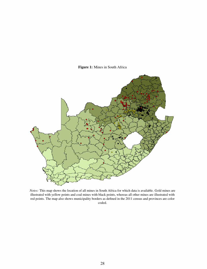
http://www.worldbank.org/en/topic/extractiveindustries/overview

http://www.worldbank.org/en/topic/extractiveindustries/overview

Figure 1: Mines in South Africa

Notes: This map shows the location of all mines in South Africa for which data is available. Gold mines areillustrated with yellow points and coal mines with black points, whereas all other mines are illustrated withred points. The map also shows municipality borders as defined in the 2011 census and provinces are color

coded.

28

Figure 2: Production of Minerals in South Africa

34

56

Ant

imon

y (k

t)

2000 2005 2010Year

68

1012

Chr

omite

(M

t)

2000 2005 2010Year

220

240

260

Coa

l (M

t)

2000 2005 2010Year

0.5

11

2C

obal

t (k

t)

2000 2005 2010Year

100

120

140

160

Cop

per

(kt)

2000 2005 2010Year

812

16D

iam

ond

cara

ts (

Mct

)

2000 2005 2010Year

250

350

450

Gol

d (t

)

2000 2005 2010Year

3545

55Iro

n or

e (M

t)

2000 2005 2010Year

4060

80Le

ad (

kt)

2000 2005 2010Year

26

10M

anga

nese

(M

t)

2000 2005 2010Year

3035

4045

Nic

kel

(kt)

2000 2005 2010Year

6070

8090

Pal

ladi

um (

t)

2000 2005 2010Year

2.2

2.6

3P

hosp

hate

(M

t)

2000 2005 2010Year

220

260

300

PG

Ms

(t)

2000 2005 2010Year

6010

014

0S

ilver

(t)

2000 2005 2010Year

Tin

(kt)

2000 2005 2010Year

600

700

800

Tita

nium

(kt

)

2000 2005 2010Year

1520

2530

Van

adiu

m (

kt)

2000 2005 2010Year

3040

5060

70Zi

nc (

kt)

2000 2005 2010Year

300

350

400

450

Zirc

oniu

m (

kt)

2000 2005 2010Year

South Africa Total Annual Production

Figure 3: South Africa Share of World Production

Ant

imon

y

1990 2000 2010Year

020

4060

8010

0C

hrom

ite

1990 2000 2010Year

Coa

l

1990 2000 2010Year

Cob

alt

1990 2000 2010Year

Cop

per

1990 2000 2010Year

Dia

mon

d ca

rats

1990 2000 2010Year

020

4060

8010

0G

old

1990 2000 2010Year

Iron

ore

1990 2000 2010Year

Lead

1990 2000 2010Year

Man

gane

se

1990 2000 2010Year

Nic

kel

1990 2000 2010Year

020

4060

8010

0P

hosp

hate

1990 2000 2010Year

Pla

tinum

1990 2000 2010Year

PG

Ms

1990 2000 2010Year

Silv

er

1990 2000 2010Year

Tin

1990 2000 2010Year

020

4060

8010

0Ti

tani

um

1990 2000 2010Year

Van

adiu

m

1990 2000 2010Year

Zinc

1990 2000 2010Year

Zirc

oniu

m

1990 2000 2010Year

South Africa % Share of Annual World Production

020

4060

8010

00

2040

6080

100

020

4060

8010

00

2040

6080

100

020

4060

8010

00

2040

6080

100

020

4060

8010

00

2040

6080

100

020

4060

8010

00

2040

6080

100

020

4060

8010

00

2040

6080

100

020

4060

8010

00

2040

6080

100

020

4060

8010

00

2040

6080

100

29

Figure 4: Police Stations in South Africa

Notes: This map shows the geographical location of all police stations in South Africa. The map also showsthe borders of the police precincts in 2003.

30

Figure 5: International Mineral Prices

(a) Low Price Minerals

0.0

001

.000

2.0

003

.000

4P

rice

(US

D/ G

ram

)

2002 2004 2006 2008 2010 2012Year

Coal ChromiteIron Ore Manganese OrePhosphate Rock Titanium

(b) Medium Price Minerals

0.0

2.0

4.0

6.0

8.1

Pric

e (U

SD

/ G

ram

)

2002 2004 2006 2008 2010 2012Year

Antimony CopperCobalt LeadNickel TinZirconium Zinc

(c) High Price Minerals

020

4060

US

D /

Gra

m

2002 2004 2006 2008 2010 2012Year

Gold PalladiumPlatinum VanadiumSilver

Notes: These graphs show the international mineral price for the minerals used in the IVanalysis.

31

Figure 6: Active Mines and Crime Rates in Mineand Non-mine Precincts

4045

5055

60C

rime

per

1000

Inha

bita

nts

210

220

230

240

250

Num

ber

of A

ctiv

e M

ines

2002 2004 2006 2008 2010 2012Year

Active Mines No MineMine within 20 km

(a) Total Crime

2025

3035

Crim

e pe

r 10

00 In

habi

tant

s

210

220

230

240

250

Num

ber

of A

ctiv

e M

ines

2002 2004 2006 2008 2010 2012Year


(b) Property Crime

1416

1820

22C

rime

per

1000

Inha

bita

nts

210

220

230

240

250

Num

ber

of A

ctiv

e M

ines

2002 2004 2006 2008 2010 2012Year


(c) Violent Crime

32

Figure 7: Matching mines and police precincts

Figure 8: Mines and Lights at Night in 2012

33

Table 1: Summary statistics

MEAN SD MIN MAX OBSA: Price SampleInternational Mineral Price (USD/gram) 16.6 20.1 0.0000024 60.6 5260Lights at Night 15.4 20.6 0 63 5260Population (1000’) 55.1 58.6 0.14 592.3 5260Active Mine 20km 2.89 4.04 0 35 5260# Start Producing 20km 0.12 0.42 0 5 4733# Stop Producing 20km 0.061 0.28 0 3 4733Total Crime per 1000 88.9 914.5 3.49 24794.3 5260Economic Crime per 1000 59.6 740.7 1.22 21531.7 5260Violent Crime per 1000 19.9 56.2 1.39 1544.7 5260Log(Total Crime per 1000) 3.71 0.70 1.25 10.1 5260Log(Economic Crime per 1000) 3.02 0.86 0.20 9.98 5260Log(Violent Crime per 1000) 2.73 0.59 0.33 7.34 5260B: Precinct SampleLights at Night 13.3 20.8 0 63 10830Population (1000’) 45.5 53.6 0.14 592.3 10830Active Mine 20km 1.66 3.77 0 36 10830# Start Producing 20km 0.062 0.29 0 5 9747# Stop Producing 20km 0.030 0.19 0 3 9747Total Crime per 1000 72.2 641.8 2.24 24794.3 10830Economic Crime per 1000 44.5 519.6 0.58 21531.7 10830Violent Crime per 1000 19.1 41.3 0 1544.7 10830Log(Total Crime per 1000) 3.66 0.77 0.80 10.1 10830Log(Economic Crime per 1000) 2.90 0.93 -0.54 9.98 10830Log(Violent Crime per 1000) 2.69 0.64 0.18 7.34 10825C: Municipality SampleMigrants’ Share of Pop 0.0015 0.0026 0 0.062 2106SADC Male Migrants’ Share of Pop 0.00056 0.0011 0 0.026 2106Male Migrants’ Share of Pop 0.0010 0.0015 0 0.035 2106Population (1000’) 210.8 482.0 6.98 4555.7 2340Active Mine 20km 2.86 5.93 0 44 2340# Start Producing 20km 0.097 0.36 0 4 2340# Stop Producing 20km 0.059 0.27 0 3 2340Total Crime per 1000 39.8 22.3 4.50 145.1 2340Economic Crime per 1000 19.2 12.0 1.44 90.1 2340Violent Crime per 1000 15.7 8.50 2.19 55.4 2340Log(Total Crime per 1000) 3.50 0.64 1.50 4.98 2340Log(Economic Crime per 1000) 2.74 0.70 0.37 4.50 2340Log(Violent Crime per 1000) 2.59 0.60 0.79 4.01 2340

Notes: This table reports summary statistics for the three main samples used in the analysis. Columns (1) through(4) reports the mean, standard deviation, minimum and maximum values of the listed variables, whereas column(5) show the number of observations. The construction of these variables are explained in sections 4.

34

Table 2: Precinct IV

Total Crime Property Crime Violent Crime

OLS 0.0284*** 0.0351*** 0.0212***(0.00604) (0.00722) (0.00478)

2SLS -0.073*** -0.088*** -0.066***(0.020) (0.022) (0.024)[0.024] [0.027] [0.027]

Reduced Form -0.00192*** -0.00230*** -0.00174***(0.000504) (0.000551) (0.000615)

First Stage 0.026***(0.0018)[0.0024]

F Statistic (one way cluster) 206.9F Statistic (two way cluster) 121.1Observations 5260

Mineral by Precinct FE Yes Yes YesYear FE Yes Yes Yes

Notes: This table reports the result of an IV regression using the world market price to instrument the numberof mines that produce a given mineral within 20 km from a precinct. The IV estimate for each of the threecrime categories (log of crime per capita in the precinct) is presented in the first row and the correspondingreduced form estimates in the second row. The first stage relationship is reported in the final row. All these re-gressions are carried out at the mineral-precinct level and include mineral by precinct fixed effects as well asyear fixed effects. Standard errors in parenthesis are clustered at the precinct and standard errors in bracketsare clustered at the precinct and the mineral-year level.

Table 3: Precinct fixed effects

OLS FE

Total Crime Total Crime Property Crime Violent CrimeActive Mine 20 km 0.0239*** -0.0171** -0.0124 -0.0184**

(0.00484) (0.00713) (0.00798) (0.00786)Observations 10830 10830 10830 10825R-Squared 0.0136 0.955 0.952 0.905Mean of Outcome 3.665 3.665 2.898 2.694

Precinct FE No Yes Yes YesYear FE No Yes Yes Yes

Notes: Column 1 presents the OLS cross-sectional results. Column 2-4 report the results of a fixed effect re-gression of the log of the local crime rate in a precinct on the number of active mines within 20 km from theprecinct, with controls for precinct and year fixed effects. Standard errors in parenthesis are clustered at theprecinct. For inclusion of the square term of the treatment variable, see Table A6. To see results for gold andcoal separately, please see Table A7.

35

Table 4: Municipality fixed effects

OLS FE

Total Crime Total Crime Property Crime Violent CrimeActive Mine 20 km 0.0193*** -0.0157** -0.0157** -0.0139


Municipality FE No Yes Yes YesYear FE No Yes Yes Yes

Notes: This table resports the results from a fixed effect regression of the log of the local crime rate in a munic-ipality on the number of active mines within 20 km from the precinct. All regressions control for municipalityand year fixed effects. Standard errors in parenthesis are clustered at the precinct.

36

Table 5: Start & Stop Producing IV


A: Start Producing (incl. all mines)

2SLS 2.323 2.746 2.182(1.890) (2.193) (1.865)

First Stage -0.000893(0.000675)

F Statistic 1.748Observations 4733

B: Start Producing (excl. new mines)

2SLS -2.086* -2.465* -1.959*(1.077) (1.294) (1.059)

First Stage 0.000994**(0.000464)


C: Stop Producing

2SLS 0.862*** 1.019*** 0.809***(0.272) (0.311) (0.308)

First Stage -0.00241***(0.000483)



Notes: This table reports the result from instrumenting production shocks (i.e. whether a particular mineralmine starts or stops producing in a given year) with the international mineral price. The outcome is the logof the crime rate in a precinct and the instrumented variable the number of mines that start or stop producinga given mineral within 20km from a precinct. Panels A instruments production starts for all mines, Panel Binstruments production starts for already existing mines and Panel C instruments mine closures for all mines.All regressions include mineral by precinct fixed effect as well as year fixed effects. Standard errors clusteredat the precinct level are reported in parenthesis.

37

Table 6: Start & Stop Producing Precinct FE

Total Crime Property Crime Violent CrimeStart Producing 20 km (excl. new) -0.00182 0.00659 -0.0138

(0.0101) (0.0115) (0.0137)Stop Producing 20 km 0.0232** 0.0280** 0.0106

(0.00999) (0.0113) (0.0124)Observations 9747 9747 9742R-Squared 0.957 0.954 0.907Mean of Outcome 3.638 2.864 2.664

Precinct FE Yes Yes YesYear FE Yes Yes Yes

Notes: This table reports the result from a fixed effect regression of the log crime rate in a precinct on the num-ber of mines that start and stops producing within 20 km from that precinct. All regressions include precinctfixed effect as well as year fixed effects. Standard errors clustered at the precinct level are reported in paren-thesis.

Table 7: Start & Stop Producing Precinct FE withlags and leads

Total Crime Property Crime Violent CrimeStop 20 km t-1 0.0243** 0.0319** 0.0159

(0.0114) (0.0132) (0.0149)Stop 20 km 0.0300** 0.0354*** 0.0193

(0.0122) (0.0133) (0.0147)Stop 20 km t+1 0.0209 0.0325** -0.00399

(0.0129) (0.0145) (0.0203)Start 20 km t-1 (excl. new) 0.00126 -0.00491 -0.00220

(0.0125) (0.0139) (0.0164)Start 20 km (excl. new) -0.0181 -0.0146 -0.0258

(0.0134) (0.0144) (0.0180)Start 20 km t+1 (excl. new) -0.00681 0.00380 -0.0215


Precinct FE Yes Yes YesYear FE Yes Yes Yes

Notes: This table reports the result from a fixed effect regression of the log crime rate in a precinct on the lagsand leads of the number of mines that start and stops producing within 20 km from that precinct. All regres-sions include precinct fixed effect as well as year fixed effects. Standard errors clustered at the precinct levelare reported in parenthesis.

38

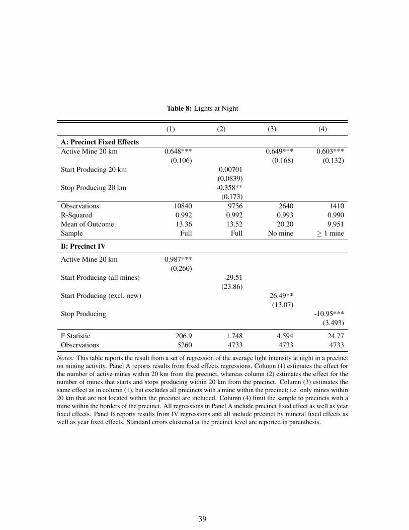
Table 8: Lights at Night

(1) (2) (3) (4)

A: Precinct Fixed EffectsActive Mine 20 km 0.648*** 0.649*** 0.603***

(0.106) (0.168) (0.132)Start Producing 20 km 0.00701

(0.0839)Stop Producing 20 km -0.358**

(0.173)Observations 10840 9756 2640 1410R-Squared 0.992 0.992 0.993 0.990Mean of Outcome 13.36 13.52 20.20 9.951Sample Full Full No mine ≥ 1 mine

B: Precinct IV

Active Mine 20 km 0.987***(0.260)

Start Producing (all mines) -29.51(23.86)

Start Producing (excl. new) 26.49**(13.07)

Stop Producing -10.95***(3.493)

F Statistic 206.9 1.748 4.594 24.77Observations 5260 4733 4733 4733

Notes: This table reports the result from a set of regression of the average light intensity at night in a precincton mining activity. Panel A reports results from fixed effects regressions. Column (1) estimates the effect forthe number of active mines within 20 km from the precinct, whereas column (2) estimates the effect for thenumber of mines that starts and stops producing within 20 km from the precinct. Column (3) estimates thesame effect as in column (1), but excludes all precincts with a mine within the precinct; i.e. only mines within20 km that are not located within the precinct are included. Column (4) limit the sample to precincts with amine within the borders of the precinct. All regressions in Panel A include precinct fixed effect as well as yearfixed effects. Panel B reports results from IV regressions and all include precinct by mineral fixed effects aswell as year fixed effects. Standard errors clustered at the precinct level are reported in parenthesis.

39

Table 9: Precinct IV heterogeneous effects bymine type


A: Open-pit mining (capital intensive)

2SLS 0.132 0.0690 0.143(0.313) (0.305) (0.385)

First Stage 0.00993***(0.00329)


B: Underground mining (labor intensive)

2SLS -0.0923*** -0.116*** -0.0548*(0.0251) (0.0293) (0.0305)

First Stage 0.0275***(0.00216)



Notes: This table reports the result from splitting the sample into precincts with primarily (defined as at leasthalf) open-pit mines and precincts with primarily underground mines. Precincts with an equal number ofopen-pit and underground mines have been excluded from the analysis. All regressions include mineral byprecinct fixed effect as well as year fixed effects. Standard errors clustered at the precinct level are reported inparenthesis.

40

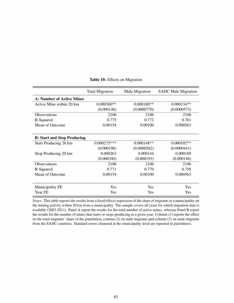
Table 10: Effects on Migration

Total Migration Male Migration SADC Male Migration

A: Number of Active MinesActive Mine within 20 km 0.000360** 0.000180** 0.000134**


B: Start and Stop ProducingStart Producing 20 km 0.000275*** 0.000148** 0.000102**

(0.000106) (0.0000582) (0.0000441)Stop Producing 20 km 0.000263 0.000144 0.000109


Municipality FE Yes Yes YesYear FE Yes Yes Yes

Notes: This table reports the results from a fixed effects regression of the share of migrants in a municipality onthe mining activity within 20 km from a municipality. The sample covers all years for which migration data isavailable (2003-2011). Panel A report the results for the total number of active mines, whereas Panel B reportthe results for the number of mines that starts or stops producing in a given year. Column (1) reports the effecton the total migrants’ share of the population, column (2) on male migrants and column (3) on male migrantsfrom the SADC countries. Standard errors clustered at the municipality level are reported in parenthesis.

41

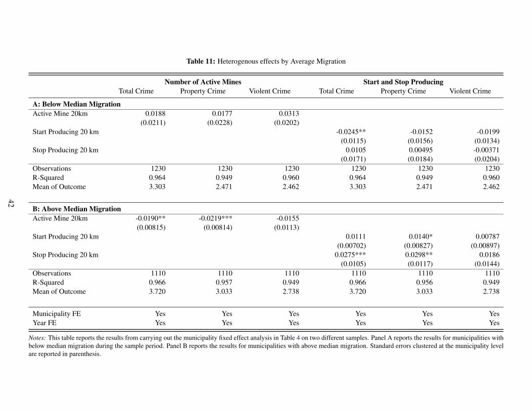
Table 11: Heterogenous effects by Average Migration

Number of Active Mines Start and Stop ProducingTotal Crime Property Crime Violent Crime Total Crime Property Crime Violent Crime

A: Below Median MigrationActive Mine 20km 0.0188 0.0177 0.0313

(0.0211) (0.0228) (0.0202)Start Producing 20 km -0.0245** -0.0152 -0.0199

(0.0115) (0.0156) (0.0134)Stop Producing 20 km 0.0105 0.00495 -0.00371

(0.0171) (0.0184) (0.0204)Observations 1230 1230 1230 1230 1230 1230R-Squared 0.964 0.949 0.960 0.964 0.949 0.960Mean of Outcome 3.303 2.471 2.462 3.303 2.471 2.462

B: Above Median MigrationActive Mine 20km -0.0190** -0.0219*** -0.0155

(0.00815) (0.00814) (0.0113)Start Producing 20 km 0.0111 0.0140* 0.00787

(0.00702) (0.00827) (0.00897)Stop Producing 20 km 0.0275*** 0.0298** 0.0186

(0.0105) (0.0117) (0.0144)Observations 1110 1110 1110 1110 1110 1110R-Squared 0.966 0.957 0.949 0.966 0.956 0.949Mean of Outcome 3.720 3.033 2.738 3.720 3.033 2.738

Municipality FE Yes Yes Yes Yes Yes YesYear FE Yes Yes Yes Yes Yes Yes

Notes: This table reports the results from carrying out the municipality fixed effect analysis in Table 4 on two different samples. Panel A reports the results for municipalities withbelow median migration during the sample period. Panel B reports the results for municipalities with above median migration. Standard errors clustered at the municipality levelare reported in parenthesis.

42

A Appendix

Table A1: Public Violence

Municipality FE Precinct FE IV

Active Mine 20km 0.00387*** 0.00510*** 0.00203(0.00120) (0.00178) (0.00672)

Observations 2340 10830 5260R-Squared 0.304 0.190 0.0221Mean of Outcome 0.0243 0.0246 0.0243

Location FE Yes Yes YesYear FE Yes Yes Yes

Notes: This table reports the results on the log of public violence per capita using the three different samples.Columns (1) and (2) report the results from the fixed effect strategy, whereas column (3) reports the resultsfrom the IV strategy. All regressions include location and year fixed effects. Standard errors clustered at thegeographical unit of observation are reported in parenthesis.

Table A2: IV excl. minerals where SA is a largeproducer


2SLS -0.0841*** -0.0956*** -0.0774***(0.0218) (0.0246) (0.0266)

Reduced Form -0.00219*** -0.00249*** -0.00201***(0.000550) (0.000615) (0.000679)

First Stage 0.0260***(0.00207)


Mineral by Mine FE Yes Yes YesYear FE Yes Yes Yes

Notes: The results in this table corresponds to those reported in Table 2, but exclude minerals for which SouthAfrica is a major producer. The minerals excluded are palladium, platinum, zirconium, vanadium, chromite,manganese ore and titanium.

43

Table A3: Effect of the number of active mineswithin a Municipality

Total Crime Property Crime Violent CrimeActive Mine -0.0182* -0.0178 -0.0132


Municipality FE Yes Yes YesYear FE Yes Yes Yes

Notes: The results in this table corresponds to those reported in Table 4, but only considers mines that arelocated within the municipality. All regressions include location and year fixed effects. Standard errors clus-tered at the municipality are reported in parenthesis.

Table A4: Crime in Levels as Outcome


A: Precinct FEActive Mine 20 km -80.38** -44.70** -53.76***


B: Precinct IV

Active Mine -342.9*** -216.7*** -175.3***(73.77) (48.99) (36.13)

Observations 5260 5260 5260R-Squared 0.0469 0.0463 0.0705Mean of Outcome 2527.2 1405.4 916.3

Notes: This table reports the results from carrying out the fixed effect (Panel A) and instrumental variable(Panel B) strategies using the number of crimes as the outcome variable. All regressions include the samefixed effects as the baseline specifications and standard errors are clustered at the precinct level.

44

Table A5: Crime in Levels (log) as Outcome


A: Precinct FEActive Mine 20 km 0.00329 0.00791 -0.0130


B: Precinct IV

Active Mine -0.450* -0.667** -0.0715(0.234) (0.308) (0.177)

Observations 4492 4492 4492R-Squared -1.048 -2.068 0.524Mean of Outcome 9.487 8.889 8.464

Notes: This table reports the results from carrying out the fixed effect (Panel A) and instrumental variable(Panel B) strategies using the log of number of crimes as the outcome variable. All regressions include thesame fixed effects as the baseline specifications and standard errors are clustered at the precinct level.

Table A6: Precinct fixed effects

OLS FE

Total Crime Total Crime Property Crime Violent CrimeActive Mine 20 km 0.0403*** -0.0250** -0.0259* -0.0249*

(0.0114) (0.0122) (0.0138) (0.0149)Active Mine 20 km square -0.000907** 0.000432 0.000735 0.000355



Notes: Column 1 presents the OLS cross-sectional results. Column 2-4 report the results of a fixed effect re-gression of the log of the local crime rate in a precinct on the number of active mines within 20 km from theprecinct, with controls for precinct and year fixed effects. Standard errors in parenthesis are clustered at theprecinct.

45

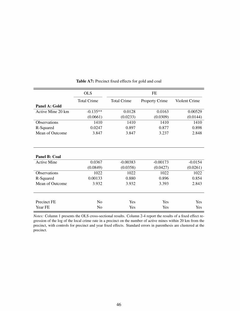
Table A7: Precinct fixed effects for gold and coal

OLS FE

Total Crime Total Crime Property Crime Violent CrimePanel A: GoldActive Mine 20 km -0.135** 0.0128 0.0163 0.00529


Panel B: CoalActive Mine 0.0367 -0.00383 -0.00173 -0.0154



Notes: Column 1 presents the OLS cross-sectional results. Column 2-4 report the results of a fixed effect re-gression of the log of the local crime rate in a precinct on the number of active mines within 20 km from theprecinct, with controls for precinct and year fixed effects. Standard errors in parenthesis are clustered at theprecinct.

46

Table A8: IV: Property Subcategories

All theft not mentioned elsewhere -0.0724***(0.0228)

Burglary at non-residential premises -0.0178(0.0217)

Burglary at residential premises -0.0719***(0.0240)

Commercial crime -0.0384*(0.0232)

Common robbery -0.135***(0.0221)

Robbery at non-residential premises -0.0250*(0.0151)

Robbery at residential premises -0.0383***(0.0131)

Shoplifting 0.0221(0.0230)

Stock-theft 0.0187(0.0183)

Theft of motor vehicle and motorcycle -0.0910***(0.0233)

Theft out of or from motor vehicle -0.0811***(0.0222)

Notes: This table reports coefficients from estimating the IV strategy for all subcategories of property crime.Each row represent a separate regression with the outcome listed in the left column. The outcome is defined asthe log of the crime rate plus one to avoid dropping data with no crime for that particular category. All regres-sions controll for time and municipality fixed effects. Standard errors clustered at the precinct are reported inparenthesis.

47

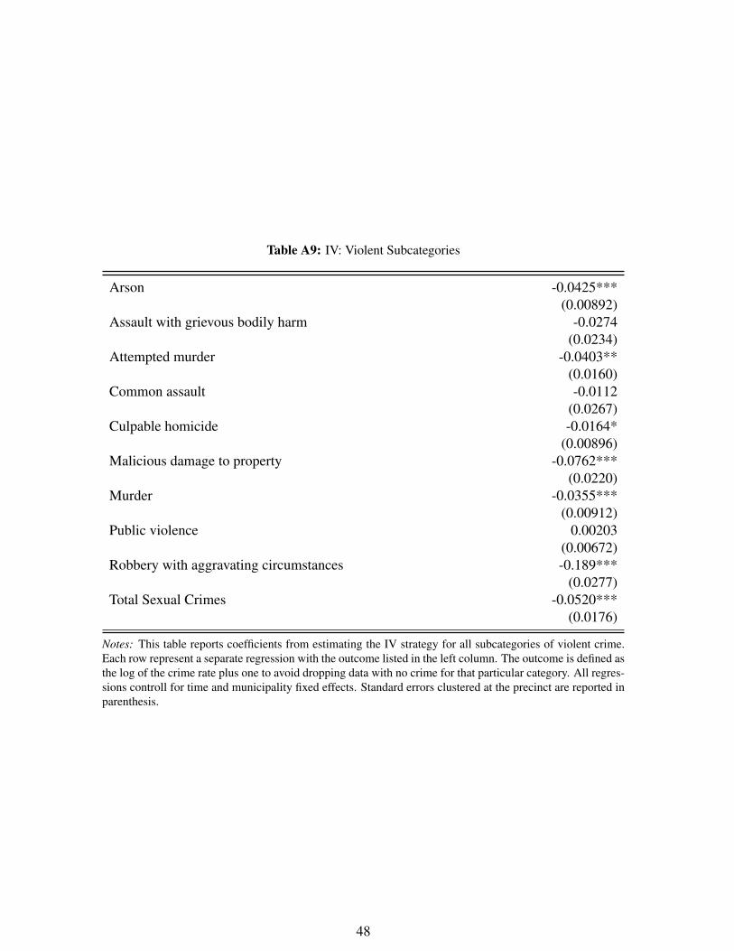
Table A9: IV: Violent Subcategories

Arson -0.0425***(0.00892)

Assault with grievous bodily harm -0.0274(0.0234)

Attempted murder -0.0403**(0.0160)

Common assault -0.0112(0.0267)

Culpable homicide -0.0164*(0.00896)

Malicious damage to property -0.0762***(0.0220)

Murder -0.0355***(0.00912)

Public violence 0.00203(0.00672)

Robbery with aggravating circumstances -0.189***(0.0277)

Total Sexual Crimes -0.0520***(0.0176)

Notes: This table reports coefficients from estimating the IV strategy for all subcategories of violent crime.Each row represent a separate regression with the outcome listed in the left column. The outcome is defined asthe log of the crime rate plus one to avoid dropping data with no crime for that particular category. All regres-sions controll for time and municipality fixed effects. Standard errors clustered at the precinct are reported inparenthesis.

48

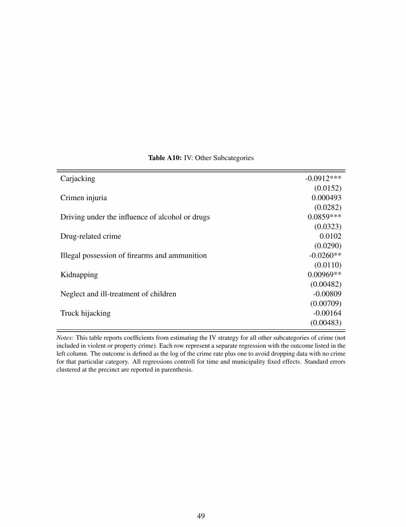
Table A10: IV: Other Subcategories

Carjacking -0.0912***(0.0152)

Crimen injuria 0.000493(0.0282)

Driving under the influence of alcohol or drugs 0.0859***(0.0323)

Drug-related crime 0.0102(0.0290)

Illegal possession of firearms and ammunition -0.0260**(0.0110)

Kidnapping 0.00969**(0.00482)

Neglect and ill-treatment of children -0.00809(0.00709)

Truck hijacking -0.00164(0.00483)

Notes: This table reports coefficients from estimating the IV strategy for all other subcategories of crime (notincluded in violent or property crime). Each row represent a separate regression with the outcome listed in theleft column. The outcome is defined as the log of the crime rate plus one to avoid dropping data with no crimefor that particular category. All regressions controll for time and municipality fixed effects. Standard errorsclustered at the precinct are reported in parenthesis.

49

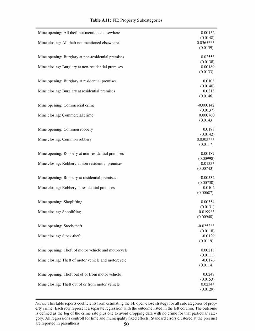
Table A11: FE: Property Subcategories

Mine opening: All theft not mentioned elsewhere 0.00152(0.0148)

Mine closing: All theft not mentioned elsewhere 0.0365***(0.0139)

Mine opening: Burglary at non-residential premises 0.0255*(0.0138)

Mine closing: Burglary at non-residential premises 0.00189(0.0133)

Mine opening: Burglary at residential premises 0.0108(0.0140)

Mine closing: Burglary at residential premises 0.0218(0.0146)

Mine opening: Commercial crime -0.000142(0.0137)

Mine closing: Commercial crime 0.000760(0.0143)

Mine opening: Common robbery 0.0183(0.0142)

Mine closing: Common robbery 0.0303***(0.0117)

Mine opening: Robbery at non-residential premises 0.00187(0.00998)

Mine closing: Robbery at non-residential premises -0.0133*(0.00743)

Mine opening: Robbery at residential premises -0.00532(0.00730)

Mine closing: Robbery at residential premises -0.0102(0.00687)

Mine opening: Shoplifting 0.00354(0.0131)

Mine closing: Shoplifting 0.0199**(0.00948)

Mine opening: Stock-theft -0.0252**(0.0118)

Mine closing: Stock-theft -0.0129(0.0119)

Mine opening: Theft of motor vehicle and motorcycle 0.00218(0.0111)

Mine closing: Theft of motor vehicle and motorcycle -0.0176(0.0114)

Mine opening: Theft out of or from motor vehicle 0.0247(0.0153)

Mine closing: Theft out of or from motor vehicle 0.0234*(0.0129)

Notes: This table reports coefficients from estimating the FE open-close strategy for all subcategories of prop-erty crime. Each row represent a separate regression with the outcome listed in the left column. The outcomeis defined as the log of the crime rate plus one to avoid dropping data with no crime for that particular cate-gory. All regressions controll for time and municipality fixed effects. Standard errors clustered at the precinctare reported in parenthesis. 50

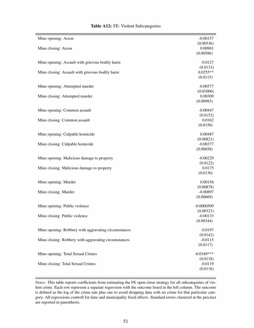
Table A12: FE: Violent Subcategories

Mine opening: Arson -0.00157(0.00536)

Mine closing: Arson 0.00901(0.00586)

Mine opening: Assault with grievous bodily harm -0.0127(0.0133)

Mine closing: Assault with grievous bodily harm 0.0255**(0.0115)

Mine opening: Attempted murder -0.00577(0.01000)

Mine closing: Attempted murder 0.00309(0.00983)

Mine opening: Common assault -0.00447(0.0152)

Mine closing: Common assault 0.0162(0.0150)

Mine opening: Culpable homicide 0.00487(0.00821)

Mine closing: Culpable homicide -0.00377(0.00658)

Mine opening: Malicious damage to property -0.00229(0.0122)

Mine closing: Malicious damage to property 0.0175(0.0130)

Mine opening: Murder 0.00156(0.00878)

Mine closing: Murder -0.00897(0.00669)

Mine opening: Public violence -0.0000509(0.00323)

Mine closing: Public violence -0.00133(0.00344)

Mine opening: Robbery with aggravating circumstances -0.0197(0.0142)

Mine closing: Robbery with aggravating circumstances -0.0115(0.0117)

Mine opening: Total Sexual Crimes -0.0349***(0.0118)

Mine closing: Total Sexual Crimes -0.0119(0.0116)

Notes: This table reports coefficients from estimating the FE open-close strategy for all subcategories of vio-lent crime. Each row represent a separate regression with the outcome listed in the left column. The outcomeis defined as the log of the crime rate plus one to avoid dropping data with no crime for that particular cate-gory. All regressions controll for time and municipality fixed effects. Standard errors clustered at the precinctare reported in parenthesis.

51

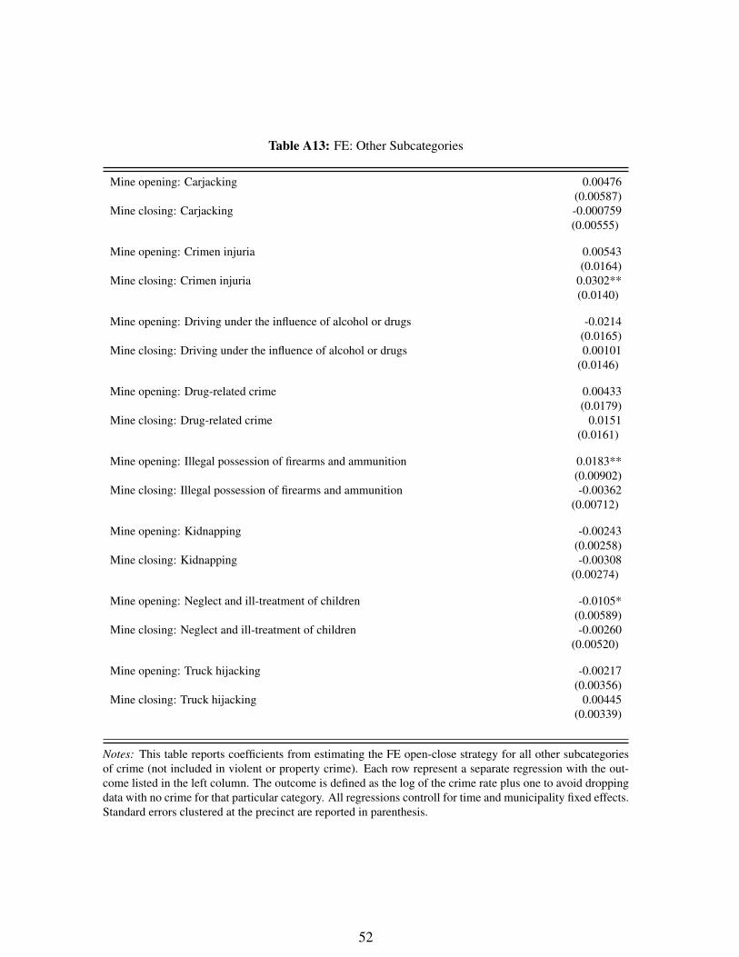
Table A13: FE: Other Subcategories

Mine opening: Carjacking 0.00476(0.00587)

Mine closing: Carjacking -0.000759(0.00555)

Mine opening: Crimen injuria 0.00543(0.0164)

Mine closing: Crimen injuria 0.0302**(0.0140)

Mine opening: Driving under the influence of alcohol or drugs -0.0214(0.0165)

Mine closing: Driving under the influence of alcohol or drugs 0.00101(0.0146)

Mine opening: Drug-related crime 0.00433(0.0179)

Mine closing: Drug-related crime 0.0151(0.0161)

Mine opening: Illegal possession of firearms and ammunition 0.0183**(0.00902)

Mine closing: Illegal possession of firearms and ammunition -0.00362(0.00712)

Mine opening: Kidnapping -0.00243(0.00258)

Mine closing: Kidnapping -0.00308(0.00274)

Mine opening: Neglect and ill-treatment of children -0.0105*(0.00589)

Mine closing: Neglect and ill-treatment of children -0.00260(0.00520)

Mine opening: Truck hijacking -0.00217(0.00356)

Mine closing: Truck hijacking 0.00445(0.00339)

Notes: This table reports coefficients from estimating the FE open-close strategy for all other subcategoriesof crime (not included in violent or property crime). Each row represent a separate regression with the out-come listed in the left column. The outcome is defined as the log of the crime rate plus one to avoid droppingdata with no crime for that particular category. All regressions controll for time and municipality fixed effects.Standard errors clustered at the precinct are reported in parenthesis.

52

extractive industries, production shocks and criminality...

Documents