extrapolating ppps and comparing icp benchmark results
TRANSCRIPT
International Comparison Program
Measuring the Size of the World Economy ICP Book
Chapter 18
Extrapolating PPPs and Comparing
ICP Benchmark Results
Paul McCarthy

2
Table of contents
Estimating PPPs for Non-benchmark Years ........................................................................................... 5
Consistency between Time and Space .................................................................................................... 5
Eurostat Rolling Benchmark Approach ................................................................................................ 10
Penn World Table ................................................................................................................................. 11
International Comparisons in World Development Indicators .............................................................. 11
Constant PPPs ....................................................................................................................................... 12
Why Extrapolations Differ from a Subsequent Benchmark in Practice................................................ 13
Assumptions about Countries with Similar Economic Structures ........................................................ 16
Effects of Changes in the Terms of Trade ............................................................................................ 18
The Balassa-Samuelson Effect.............................................................................................................. 19
Differences between the 2005 and 2011 Benchmarks Caused by Changes in Methodology ............... 20
Improving Extrapolation Methods ........................................................................................................ 20
Estimating PPPs for Nonparticipating Countries .................................................................................. 21
Comparing ICP Benchmark Results ..................................................................................................... 21
Conclusion ............................................................................................................................................ 26
Annex A. World Bank Atlas Method.................................................................................................... 27
Annex B. Transitivity of PPPs Extrapolated Using the GDP Deflator Method .................................... 29
Annex C. Estimation of PPPs for Nonbenchmark Economies ............................................................. 31
References ............................................................................................................................................. 36
Notes ..................................................................................................................................................... 38

3
The International Comparison Program (ICP) provides estimates of the gross domestic product (GDP)
and its main expenditure components for most countries in the world expressed in a common currency
and at consistent price levels for a specific reference year (2005 for the estimates in this book). In this
respect, the estimates are different from those more commonly available in a country’s national
accounts, in which the evolution of an economy over time can be analyzed through the annual (or
quarterly) time series data that are available. The output of the ICP is often referred to as a ―snapshot‖
of the relationships between the economies of participating countries because the data relate to the
level of economic activity in each country in a single reference year.
The 2005 ICP provided detailed purchasing power parity (PPP) data for 146 countries. Because of the
cost of conducting a worldwide project such as the ICP, the PPPs for most countries are produced
infrequently. For example, the 2011 ICP round is taking place six years after the 2005 ICP. But PPPs
and related data (real expenditures and price level indexes, PLIs) for some countries are available
more frequently. For example, Eurostat, the European Union’s statistical office, produces annual PPPs
for its member and candidate countries using a ―rolling benchmark‖ approach,1 and the Organisation
for Economic Co-operation and Development (OECD) currently produces PPPs, real expenditures,
and PLIs for its non-European member countries every three years.
The availability of firm PPP-based expenditure data for 2005 for so many countries has resulted in
increased interest in PPPs by analysts engaged in worldwide comparisons of economic activity. One
outcome has been that analysts want to obtain PPPs and real expenditures for countries that did not
participate in the 2005 ICP. In past ICP rounds, PPPs and real expenditures for nonparticipating
countries have been estimated using regression models. The number of countries for which these
imputed estimates were required in the 2005 ICP was lower than in previous rounds but, even so,
PPPs were estimated for 42 countries in addition to the 146 countries that participated in the 2005
ICP. In practice, though, the accuracy of the results from this imputation procedure depends on a
number of assumptions, and so the results are not as accurate as the estimates for the countries that
participated in the ICP. The demand for these data has been met by imputing PPPs for these 42
countries using a regression model. Another outcome has been the need for PPPs that are more up-to-
date than those from the 2005 ICP. As a consequence, the 2005 PPPs have been extrapolated to later
years for countries not included in the annual Eurostat PPP Programme. One result is that the PPPs
extrapolated for each out-year are being used as though they form a time series that can be applied
directly to the annual values of national accounts aggregates such as GDP. Despite the shortcomings
involved, many research studies are based on this type of procedure because the only alternative is to
use exchange rates, which, for obvious reasons, is not a viable method for most international
comparisons.
Various organizations provide estimates of PPPs for years other than benchmark years. The OECD
extrapolates PPPs for GDP from its latest benchmark for each successive year because of the demand
by users for annual PPPs. It also interpolates between past benchmarks to form a time series of annual
PPPs and real expenditures. The University of Pennsylvania’s Center for International Comparisons
of Production, Income and Prices compiles the Penn World Table (PWT), which provides an annual
series of PPP-based real expenditures and PLIs to meet the demand for this type of data. However,
problems arise in using PPPs as though they are times series because PPPs are designed for
comparing economic activity between countries (i.e., a spatial comparison) rather than comparing
changes across time, which is the more common method of analyzing national accounts.
Conceptually, it is impossible to maintain consistency simultaneously across both space and time
except under very restrictive assumptions. A time series of PPPs may provide plausible results

4
provided that the economic structures of the countries involved in the comparison do not change
rapidly. However, distorted results are likely to be obtained if the economies of the countries are
dissimilar or the economic structures of the countries are changing at very different rates (e.g., the
United States and China in recent years).
This chapter covers in some detail the issues involved in using PPPs in a time series mode. The goal is
to alert users of PPP-related data to the types of assumptions that underlie extrapolated and backcast
PPPs and real expenditures so that they can make informed decisions about the data they are using. It
is clear that, despite their shortcomings when used as a time series, PPPs still provide much more
firmly based international comparisons for most purposes than the oft-used alternative of market
exchange rates.
Before readers venture further into a chapter that introduces some fairly complex concepts, it may be
helpful to clarify some of the terms used in the context of this chapter. The tables in a time series of
national accounts are generally expressed in terms of values, but these values may be expressed in
terms of ―current prices‖ or ―constant prices.‖ Values expressed in terms of current prices may be
referred to as ―current values‖ or ―current price values‖ or even just ―values,‖ with ―current prices‖
being understood from the context. A value can be thought of as being obtained by multiplying the
quantity of a particular product by its unit price. For example, the value of 100 tons of wheat at a price
of $250 per ton would be $25,000. As prices change over time, the current value will change even if
the underlying quantity remains the same, and so a time series of annual current values includes the
combined effects of quantity changes and price changes from year to year. For many types of
analysis, it is useful to identify the underlying quantity of activity. However, once a value includes
more than one product, it is impossible to obtain meaningful quantities (the old problem of being
unable to add apples and oranges). Therefore, a time series of ―constant price values‖ is estimated by
removing the effects on the current values of price changes over time. The mechanics of this process
may vary significantly but can be thought of as dividing a price index of relevant products into the
corresponding current values. These price indexes are generally called ―deflators.‖ In algebraic terms:
constant price value = current value/deflator.
It is necessary to specify a particular ―base year‖ in estimating a series of constant price values. The
level of the constant price value for each component of GDP in the base year will be equal to its
current value, but the constant price values in other years will be different from the current values
(unless there is no change in prices from the base year to the year being considered). Constant price
values are often referred to in the national accounts as ―volumes.‖ Changes in constant price values
from year to year may be linked together to form a ―chained volume.‖ Volumes are estimated for
many components of GDP and then summed to obtain the volume of GDP. In the ICP, the current
values of GDP and its components are generally described as values expressed in ―local currency
units‖ or ―national currency units‖ to stress the fact that they are in units not comparable from one
country to another. These values are divided by PPPs to express them in terms of a common currency,
with the resultant values called ―real expenditures‖ (sometimes also referred to as ―volumes‖) because
the effects of price level differences across countries have been removed. In the ICP, values in local
currency units that have been converted to a common currency by dividing them by exchange rates
are called ―nominal values‖ because they still include the effects of price level differences between
the countries as well as the volume differences.

5
Estimating PPPs for Non-benchmark Years
The statistical framework for national accounts is provided in the System of National Accounts 2008
(Commission of the European Communities et al. 2008). Chapter 15 on price and volume measures
describes the techniques most commonly used in estimating volumes. The chapter also describes
some of the issues involved in obtaining PPPs and real expenditures for international comparisons,
and paragraphs 15.232 and 15.233 describe how PPPs are usually estimated for non-benchmark years:
15.232 The method commonly used to extrapolate PPPs from their benchmark year to another
year is to use the ratio of the national accounts deflators from each country compared with a
numeraire country (generally the United States of America) to move each country’s PPPs
forward from the benchmark. The PPPs derived are then applied to the relevant national
accounts component to obtain volumes [real expenditures] expressed in a common currency for
the year in question.
15.233 Theoretically, the best means of extrapolating PPPs from a benchmark year would be to
use time series of prices at the individual product level from each country in the ICP to
extrapolate the prices of the individual products included in the ICP benchmark. In practice, it
is not possible to use this type of procedure in extrapolating PPP benchmarks because the
detailed price data needed are not available in all the countries. Therefore, an approach based
on extrapolating at a macro level (for GDP or for a handful of components of GDP) is generally
adopted. Leaving aside the data problems involved in collecting consistent data from all the
countries involved, a major conceptual question arises with this process because it can be
demonstrated mathematically that it is impossible to maintain consistency across both time and
space. In other words, extrapolating PPPs using time series of prices at a broad level such as
GDP will not result in a match with the benchmark PPP-based estimates even if all the data are
perfectly consistent.
Consistency between Time and Space
The nature of the differences between GDP volume growth rates, as measured by the time series
national accounts and as implied by PPP benchmarks, has been investigated intermittently since the
initial phases of the ICP. Examples of such investigations are found in Khamis (1977) and chapter 8
of the official report of the 1975 ICP (Statistical Office of the United Nations and World Bank 1982).
This issue was very important then because ICP rounds were run only once every five years in the
1970s, and the differences between ―actual results‖ (i.e., PPP benchmark estimates) and ―extrapolated
results‖ (i.e., extrapolating from the latest benchmark using time series) were significant in many
cases. The broad reasons for these differences are well known and include issues such as the different
product baskets used in the time series national accounts deflators and in estimating the PPPs,
different computational methods, different weighting patterns, and so forth.
More recently, these issues have been investigated further because of the growing interest in
international comparisons over time. An interesting analysis of the problems in maintaining
consistency in PPPs simultaneously across time and space has been presented by Dalgaard and
Sørensen (2002). They demonstrate that, conceptually, it is impossible to maintain such consistency
(except under the completely unrealistic condition of having a common fixed price vector in all
periods, which implies that the price structure in every country is identical in each period). This
conclusion holds no matter which index number formulas are chosen for estimating both the time
6
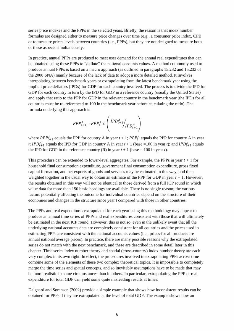
series price indexes and the PPPs in the selected years. Briefly, the reason is that index number
formulas are designed either to measure price changes over time (e.g., a consumer price index, CPI)
or to measure prices levels between countries (i.e., PPPs), but they are not designed to measure both
of these aspects simultaneously.
In practice, annual PPPs are produced to meet user demand for the annual real expenditures that can
be obtained using these PPPs to ―deflate‖ the national accounts values. A method commonly used to
produce annual PPPs is based on a macro approach (as outlined in paragraphs 15.232 and 15.233 of
the 2008 SNA) mainly because of the lack of data to adopt a more detailed method. It involves
interpolating between benchmark years or extrapolating from the latest benchmark year using the
implicit price deflators (IPDs) for GDP for each country involved. The process is to divide the IPD for
GDP for each country in turn by the IPD for GDP in a reference country (usually the United States)
and apply that ratio to the PPP for GDP in the relevant country in the benchmark year (the IPDs for all
countries must be re–referenced to 100 in the benchmark year before calculating the ratio). The
formula underlying this approach is
=
where equals the PPP for country A in year t + 1;
equals the PPP for country A in year
t; equals the IPD for GDP in country A in year t + 1 (base =100 in year t); and
equals
the IPD for GDP in the reference country (R) in year t + 1 (base = 100 in year t).
This procedure can be extended to lower-level aggregates. For example, the PPPs in year t + 1 for
household final consumption expenditure, government final consumption expenditure, gross fixed
capital formation, and net exports of goods and services may be estimated in this way, and then
weighted together in the usual way to obtain an estimate of the PPP for GDP in year t + 1. However,
the results obtained in this way will not be identical to those derived from a full ICP round in which
value data for more than 150 basic headings are available. There is no single reason; the various
factors potentially affecting the outcome for individual countries depend on the structure of their
economies and changes in the structure since year t compared with those in other countries.
The PPPs and real expenditures extrapolated for each year using this methodology may appear to
produce an annual time series of PPPs and real expenditures consistent with those that will ultimately
be estimated in the next ICP round. However, this is not so, even in the unlikely event that all the
underlying national accounts data are completely consistent for all countries and the prices used in
estimating PPPs are consistent with the national accounts values (i.e., prices for all products are
annual national average prices). In practice, there are many possible reasons why the extrapolated
series do not match with the next benchmark, and these are described in some detail later in this
chapter. Time series index number theory and spatial (cross-country) index number theory are each
very complex in its own right. In effect, the procedures involved in extrapolating PPPs across time
combine some of the elements of these two complex theoretical topics. It is impossible to completely
merge the time series and spatial concepts, and so inevitably assumptions have to be made that may
be more realistic in some circumstances than in others. In particular, extrapolating the PPP or real
expenditure for total GDP can yield some quite misleading results at times.
Dalgaard and Sørensen (2002) provide a simple example that shows how inconsistent results can be
obtained for PPPs if they are extrapolated at the level of total GDP. The example shows how an

7
implausible outcome arises when PPPs for GDP are extrapolated from a benchmark year even when
prices for similar products are moving identically in each of two the countries being compared. It
could be extended to cover the situation in which PPPs are extrapolated for only a handful of broad
aggregates, such as those for household final consumption expenditure, government final
consumption expenditure, gross fixed capital formation, and net exports of goods and services.
The example provided by Dalgaard and Sørensen (2002) assumes that the two countries involved
(country A and country B) have the same GDP and price level in year t. Expenditure on GDP consists
of two products, ―goods‖ and ―services.‖ Goods comprise 80 percent of GDP in country A but only 20
percent in country B. Conversely, services are 20 percent of GDP in country A and 80 percent in
country B. The prices (in local currency units) for goods in year t are 1.00 in each of countries A and
B, and they remain the same in both cases in the next benchmark year (referred to as year t + 1). The
prices for services are 1.00 in year t in both countries, but they double to 2.00 in year t + 1 in both
countries, whereas there is no change in the quantities of goods and services produced between years t
and t + 1. The details are summarized in table 18.1.
Table 18.1 Values and Prices of Goods and Services
Product
Country A Country B
GDP,
year t
Price,
year t
Price,
year t + 1
GDP,
year t + 1
GDP,
year t
Price,
year t
Price,
year t + 1
GDP,
year t + 1
Goods 80 1.00 1.00 80 20 1.00 1.00 20
Services 20 1.00 2.00 40 80 1.00 2.00 160
GDP 100 120 100 180
Source: The author.
The PPPs for both products are 1.00 in year t (1.00/1.00 for goods and for services), which means that
the PPP for GDP is also 1.00 in that year. The PPPs for both products are 1.00 in year t + 1 (1.00/1.00
for goods and 2.00/2.00 for services), and so the PPP for GDP remains equal to 1.00 in year t + 1. The
PPPs between countries A and B are 1.00 for both goods and services in year t and year t + 1.
Therefore, the PPPs for GDP in both years must also be 1.00. Table 18.2 summarizes the PPPs.
Table 18.2 PPPs of Goods and Services
Product PPP (A/B),
year t
PPP (A/B),
year t + 1
Goods 1.00 (= 1.00/1.00) 1.00 (= 1.00/1.00)
Services 1.00 (= 1.00/1.00) 1.00 (= 2.00/2.00)
GDP 1.00 1.00
Source: The author.
The volume of GDP in year t + 1 with year t as the base year can be calculated by deriving the price
deflators for goods and for services in both countries and then dividing these deflators into the
corresponding values and summing the results to obtain the volume of GDP. The price deflators in
year t are equal to 100.0 because that is the base year. In year t + 1, they are obtained by dividing the
year t + 1 price for goods and for services by the corresponding price in year t (i.e., 1.00/1.00 * 100 =
100.0 for goods and 2.00/1.00 * 100 = 200.0 for services in both countries). Table 18.3 provides
details of the steps involved in obtaining the volumes of goods and services and of GDP in year t + 1.
8
Table 18.3 Volumes of Goods and Services
Product
Country A Country B
GDP
,
year
t
Price
deflator,
year t
Price
deflator,
year t +
1
Volume,
year t + 1
GDP,
year t
Price
deflator,
year t
Price
deflator,
year t +
1
GDP,
year t + 1
Goods 80 100.0 100.0 80 20 100.0 100.0 20
Services 20 100.0 200.0 20
(= 40/200.0
*100.0)
80 100.0 200.0 80
(= 160/200.0
*100.0)
GDP volume 100 100 100 100
Source: The author.
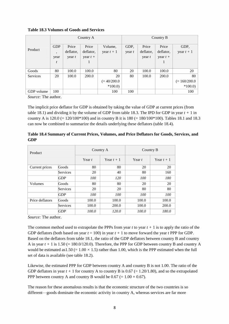
The implicit price deflator for GDP is obtained by taking the value of GDP at current prices (from
table 18.1) and dividing it by the volume of GDP from table 18.3. The IPD for GDP in year t + 1 in
country A is 120.0 (= 120/100*100) and in country B it is 180 (= 180/100*100). Tables 18.1 and 18.3
can now be combined to summarize the details underlying these deflators (table 18.4).
Table 18.4 Summary of Current Prices, Volumes, and Price Deflators for Goods, Services, and
GDP
Product Country A Country B
Year t Year t + 1 Year t Year t + 1
Current prices Goods 80 80 20 20
Services 20 40 80 160
GDP 100 120 100 180
Volumes Goods 80 80 20 20
Services 20 20 80 80
GDP 100 100 100 100
Price deflators Goods 100.0 100.0 100.0 100.0
Services 100.0 200.0 100.0 200.0
GDP 100.0 120.0 100.0 180.0
Source: The author.
The common method used to extrapolate the PPPs from year t to year t + 1 is to apply the ratio of the
GDP deflators (both based on year t = 100) in year t + 1 to move forward the year t PPP for GDP.
Based on the deflators from table 18.1, the ratio of the GDP deflators between country B and country
A in year t + 1 is 1.50 (= 180.0/120.0). Therefore, the PPP for GDP between country B and country A
would be estimated as1.50 (= 1.00 × 1.5) rather than 1.00, which is the PPP estimated when the full
set of data is available (see table 18.2).
Likewise, the estimated PPP for GDP between country A and country B is not 1.00. The ratio of the
GDP deflators in year t + 1 for country A to country B is 0.67 (= 1.20/1.80), and so the extrapolated
PPP between country A and country B would be 0.67 (= 1.00 × 0.67).
The reason for these anomalous results is that the economic structure of the two countries is so
different—goods dominate the economic activity in country A, whereas services are far more

9
important than goods in country B, and the prices of services have changed markedly compared with
those for goods.
It is important to note that a different set of results would be obtained if the PPPs for individual
components of GDP (i.e., each basic heading) were extrapolated using the relevant price changes. The
basic heading PPPs could then be weighted together to obtain PPPs for higher-level expenditure
aggregates using the same types of processes as in a full ICP round. In the example just given, the
price changes for goods and for services are identical in both countries. Therefore, extrapolating the
year t prices for each of the two components of GDP and producing PPPs for both in year t + 1 would
result in PPPs of 1.00 for goods and for services. As a result, aggregating them to a PPP for GDP
would produce the same results for GDP as those shown in table 18.2 (i.e., the PPP for GDP would be
1.00 in both year t and year t + 1). In practice, the best results from an extrapolation procedure would
be obtained if the PPPs for each of the 155 ICP basic headings were extrapolated individually using
the relationship between the price relatives for each basic heading in each country and those in a
reference country (see Biggeri and Laureti 2011).
A technique that is used in practice as a compromise between the extremes of extrapolating at the
basic heading level or for GDP in total is to extrapolate PPPs at some intermediate level between the
basic heading and GDP (e.g., for major aggregates such as household final consumption expenditure,
government final consumption expenditure, gross fixed capital formation, and net exports of goods
and services). In such a case, the PPPs extrapolated at this intermediate level are then weighted
together to estimate a PPP for GDP. The time series in the PWT are based on this type of technique,
which overcomes some of the significant differences in economic structure between countries.
However, it is important to note that extrapolating at the level of total household final consumption
expenditure using either the national accounts deflator for this aggregate or the CPI will produce
different results from those obtained by extrapolating PPPs for each basic heading within this
aggregate and then weighting them together to provide a PPP for total household final consumption
expenditure.
Extrapolating at levels of aggregation above the basic heading, such as total GDP, yields results that
are reference country–invariant. In other words, the choice of reference country should not affect the
results obtained using extrapolation methods based on applying price indicators to national accounts
values above the basic heading level. However, the process of extrapolating at the level of GDP
depends on a number of assumptions about the conceptual and practical features of the data. For
example, it is assumed that the reference country and the other country in the extrapolation have
similar economic structures and that their economies are evolving in a similar manner. On a practical
level, in compiling their national accounts countries follow the standards set out in the System of
National Accounts (SNA) to varying degrees. Even in countries that closely follow the SNA
standards, the national accounts will potentially differ in some ways that may be significant when
deflators are used to extrapolate PPPs. For example, the source data available may lead to
inconsistencies in the ways in which some estimates are calculated, or the statistical techniques used
in some countries may differ in others, with an impact on the consistency of the respective GDP
deflators. A common difference is that some countries use hedonic techniques to varying degrees to
adjust prices for quality change in products such as computers, motor vehicles, or houses, and the use
of ―output indicators‖ to estimate volumes (such as for surgical procedures) varies significantly across
countries. In such cases, extrapolating PPPs using changes in GDP deflators can produce distorted
results because of the effects of these different statistical treatments on these deflators in different
countries.

10
Eurostat Rolling Benchmark Approach
As noted, Biggeri and Laureti (2011) have concluded that the best means of extrapolating PPPs is to
individually extrapolate the PPPs for each basic heading using time series price indexes. Eurostat uses
this type of procedure in its ―rolling benchmark approach.‖ The rolling benchmark is based on pricing
part of the product lists each half-year within a three-year cycle and extrapolating them to subsequent
years using time series price indexes that are specific to each basic heading.
Eurostat describes the process in its methodological manual (Eurostat and OECD 2005):
2.24 The rolling benchmark approach facilitates annual comparisons as follows. The starting
point is the matrix of basic heading PPPs by participating country for the reference year, t. In
the subsequent year, t + 1, some of the basic heading PPPs are replaced by new PPPs calculated
using prices collected during t + 1, while the basic heading PPPs that have not been replaced
are advanced to t + 1 using temporal adjustment factors specific to these basic headings. All the
basic heading PPPs in the matrix now refer to t + 1. Aggregating the matrix with expenditure
weights for t + 1 gives PPPs and real final expenditures for each level of aggregation up to the
level of GDP with which a comparison can be made for the new reference year, t + 1. By
continuing the cycle of replacement, extrapolation and aggregation through t + 2, t + 3, t + 4,
etc., comparisons can be made for the reference years t + 2, t + 3, t + 4, etc. As over a third of
all basic heading PPPs are recalculated each year, all the basic heading PPPs in the matrix for
any given reference year have been replaced, at least once, during the 36 months prior to its
close.
Most basic headings within household final consumption expenditure are managed in this way,
although prices for rents (actual and imputed) are collected every year because of the difficulties in
obtaining consistent time series of prices to extrapolate the PPPs for rents. Likewise, price data for
compensation of employees are collected annually. Initially, prices were collected for gross fixed
capital formation (equipment goods and construction projects) every year. However, this changed
after 2005 to a biannual price collection to reduce costs. National accounts expenditures at the basic
heading level are collected annually, as are annual average exchange rates and data on average annual
resident population. Spatial adjustment factors are estimated in those countries in which the PPP
surveys cover only part of the country (e.g., the capital city).
Household final consumption expenditure is split into six surveys, and prices are collected for the
basic headings in each group during a half-year. The six groups and the period for which prices were
collected for the 2005 round are:
01. Food, drink, and tobacco first half of 2003
02. Personal appearance second half of 2003
03. House and garden first half of 2004
04. Transport, restaurants, and hotels second half of 2004
05. Services first half of 2005
06. Furniture and health second half of 2005
The main advantages of the rolling benchmark are that reliable annual PPPs can be produced, costs
are reduced, and national statistics offices can plan on a regular work cycle for their staff collecting
prices.
11
Penn World Table
The Penn World Table (PWT) is maintained by the Center for International Comparisons of
Production, Income and Prices at the University of Pennsylvania. It provides a time series of PPP-
based national accounts data for more than 180 countries from 1950. The PPPs and real expenditures
in the PWT are estimated by extrapolating and backcasting PPP-based estimates from the ICP (the
―benchmark‖). They are calculated at an intermediate stage between the detailed rolling benchmark
approach adopted by Eurostat and the broad--based approach of using either GDP volume growth to
extrapolate real expenditures on GDP or relative changes in GDP deflators to extrapolate the PPPs for
GDP. In this way, they provide a compromise between the problems caused by extrapolating at the
level of GDP (see the earlier discussion of the consistency between time and space) and the detailed
data required to extrapolate PPPs for every basic heading and then weighting them together to obtain
a PPP for GDP.
The starting point for the latest PWT time series (PWT 7.1) is the global set of basic heading PPPs
and expenditures from the 2005 ICP. PPPs are estimated for actual consumption (C), collective
government consumption (G), gross fixed capital formation (I), and net exports of goods and services.
In earlier versions of the PWT, the Geary-Khamis (GK) method was used so that the results were
additive. Therefore, GDP could be estimated as the sum of these four major components. PWT 7.1
integrates the 2005 ICP into the estimates and produces its preferred series using a variant of the Gini-
Éltetö-Köves-Szulc (GEKS) aggregation method for the initial shares in 2005 and its current price
series in earlier years. The reference PPPs for C, G, and I for 2005 are moved backward and forward
from 2005 by the changes in the prices of each of these major components for each country and
aggregated to an estimate of ―domestic absorption‖ (also referred to at times in national accounting as
―domestic final demand‖). The international trade balance is treated separately and then combined
with domestic absorption to provide the estimate for GDP. As in previous versions, the PWT provides
current and constant price estimates of the shares of consumption, investment, and government to
GDP.
International Comparisons in World Development Indicators
International comparisons are published regularly by the World Bank in its annual publication World
Development Indicators (WDI). Three different methodologies are used in converting some major
national accounts aggregates—gross national income2 (GNI) or gross domestic product—into a
common currency (U.S. dollars) to compare them across countries. In table 1.1 of the 2010 issue, size
of the economy, and table 1.6, key indicators for other economies, GNI is expressed in U.S. dollars
using the World Bank’s Atlas method (an adjusted exchange rate method rather than PPPs that is
described in the next paragraph) and also by using PPPs extrapolated to the reference year (2008 in
the 2010 edition of the WDI). In table 4.2, structure of output, in the 2010 edition of the WDI, the
levels of GDP for countries are expressed in U.S. dollars using exchange rates to convert them from
each country’s national currency into U.S. dollars (World Bank 2010).
In effect, the Atlas method produces smoothed exchange rates with some additional adjustments for
relative differences in inflation rates. The goal is ―to reduce the impact of exchange rate fluctuations
in the cross-country comparison of national incomes‖ (World Bank 2010). Briefly, the first step is to
take a three-year moving average of the country’s exchange rate (based on the current year plus the
two preceding years) and adjust it for differences in the GDP deflator between the country and those

12
in Japan, the United Kingdom, the United States, and the Euro Area. Clearly, it is essentially an
exchange rate method of adjusting values into a common currency, albeit one that removes the effects
of short-term volatility in the exchange rates. As a result, it suffers from the problem that, like regular
exchange rates, it does not remove the effects of differences in price levels between countries. Despite
this shortcoming, exchange rate methods are more appropriate than PPPs for some international
comparisons in limited circumstances. The WDI Atlas method is described in detail in annex A of this
chapter.
The estimates of GNI adjusted to a common currency by PPPs are based on the PPPs from the 2005
ICP extrapolated to the latest reference year using the macro approach (described in the earlier section
on consistency between time and space) of applying to the 2005 PPP the ratio of the GDP deflators
for each country in turn to the GDP deflator for the United States in the reference year.
Two features of the ICP since its inception almost a half-century ago have been the gradual increase
in the number of countries participating in each round and the methodological developments over
time, particularly in the 2005 ICP when new methods of specifying products and linking regions were
introduced. In addition, some countries have dropped out of the program between one round and the
next and then participated again in a subsequent round. As a result, for many countries outside the
Eurostat-OECD region, it has been difficult to interpolate PPPs between adjoining rounds. Some
analysts have used the imputed PPPs for nonparticipating countries as a benchmark (or benchmarks)
for interpolation, while others have simply backcast from the latest ICP round and ignored the PPPs
available from earlier rounds. The 2011 ICP will build on the 2005 round by providing a new
benchmark for almost all the countries that participated in 2005, using very similar methods so that
the effects of methodological change will be less pronounced than was the case previously. Therefore,
it will be possible to assess the impact of simple backcasting the 2011 PPPs (e.g., using the volume
changes in a country’s national accounts) against the benchmarks provided by the 2005 ICP.
Constant PPPs
One way suggested to maintain consistency in real expenditures simultaneously across countries and
across time is to use a single year as a benchmark for a time series. The national accounts values for
the base year are adjusted to a common currency using PPPs, and then the growth rates in GDP
volumes are applied to these base year values to obtain a series of real expenditures for years before
or after the base year. By definition, the percentage changes in these real expenditures on GDP for any
individual country are identical to those published by that country in its time series of GDP volumes.
This type of comparison is generally referred to as being estimated using ―constant PPPs.‖ In fact, the
real expenditures series generated by this type of process are broadly equivalent to a fixed-base time
series of volumes, and they suffer from the same kinds of shortcomings as these types of volumes.
An assumption underlying this estimation is that the relative levels of the real expenditures in the
chosen base year are relevant to all the other years in the series. However, in practice economic
structures (both prices and volumes) change at different rates in different countries. As a result,
comparing the relative levels of real expenditures in different countries using this type of data will
yield results that are potentially very different, depending on which year is chosen as the base year.
There is no way to select an ideal base year because the relationships between countries are changing
so rapidly. For example, over the last few years the economic growth in most European countries has
been much lower than that in most Asian countries. Therefore, using 2011 as a base year would result

13
in Asian countries being closer to the European countries for every year in the series than would be
the case if 2005 were used as the base year. In other words, the relativities between countries for all
years in the series are highly dependent on the base year chosen. In this respect, a time series at
constant PPPs is similar to a set of volumes by industry within a country when they have been
estimated using a fixed-base year. In such a case, the relationships within each year between the
volumes of gross product in each industry will depend on the base year chosen because the economic
structure of a country changes over time.
One use of these series based on ―constant PPPs‖ is to estimate regional totals (and therefore growth
rates in regional real expenditures). However, the percentage changes in a regional total will vary
depending on the base year chosen for the constant PPPs in the same way that the percentage changes
in GDP volumes will vary for an individual country when a base year is changed in a fixed-base
volume series.
Why Extrapolations Differ from a Subsequent Benchmark in Practice
PPPs can be extrapolated at any level, ranging from the basic heading up to GDP, with the more
detailed methods likely to produce better results. However, the broader levels are more likely to be
used in practice because of the lack of time series price data at the basic heading level that are
consistent across countries. The first part of this chapter showed that extrapolation methods based on
GDP or its high-level aggregates such as household final consumption expenditure should not be
expected to produce PPPs that match those from a new benchmark year. However, the fact remains
that there is a demonstrated user need for PPPs to be produced frequently (preferably annually), and
so it is essential to use extrapolation techniques, even though experience over the last decade or so has
shown that one needs to understand how the PPPs extrapolated from one benchmark year will differ
from the following benchmark.
In practice, some reasonable results have been obtained using broadly based extrapolation procedures,
but it is more common that, for at least some of the countries involved, the extrapolated PPPs will
differ significantly from a subsequent benchmark round for a number of reasons. In some cases, it
may be possible to identify a single underlying reason that is largely responsible for such differences,
but usually several factors are involved, and they may change over time or for different pairs (or
groups) of countries. The following list is a summary of the potential issues affecting the reliability of
the outcomes. Some of these issues are discussed in more detail in other sections in this chapter. They
have been classified under two headings, ―general‖ and ―extrapolation above the basic heading level.‖
The ―general‖ heading has been applied to those issues that have an impact on PPP and real
expenditure estimation and extrapolation no matter whether they are at the basic heading level or at a
more aggregated level (i.e., GDP in total or for major components of GDP such as household final
consumption expenditure and so forth, which are then aggregated to GDP). The heading
―extrapolation above the basic heading level‖ covers those issues that would not affect the results
obtained by extrapolating PPPs at the basic heading level and then weighting them to higher-level
aggregates, but that do have an impact on the outcomes obtained from extrapolating PPPs for GDP or
its major aggregates.

14
General
The products to be priced in the ICP are carefully defined to ensure comparability between
countries, but the products priced in the time series used in estimating the volumes in a
country’s national accounts are selected on the basis that they are the most representative
products available in a country. In addition, the set of prices used in a country’s time series
price indexes is much broader than those that can be included in the ICP.
The prices in a country’s time series price indexes (e.g., the CPI) are adjusted for quality
changes over time, and countries do not use common methods to adjust for these changes.
For example, hedonic methods are used to a different extent across countries (or not at all in
many countries), with the result that the quality-adjusted time series are not consistent across
countries. In particular, the U.S. Bureau of Economic Analysis uses hedonic methods more
extensively in estimating the national accounts deflators than virtually all other countries.
Therefore, if the price changes over time in the U.S. GDP deflator are lower than those in
other countries because of using hedonics, then their price levels extrapolated forward from
a benchmark year would be too high compared with those of the United States, which is
commonly used as the reference country.
In the national accounts, very few countries adjust their volumes of nonmarket services for
productivity changes. Therefore, differences in productivity over time in different countries
will be reflected in the GDP deflators as part of the price changes, leading to an
inconsistency between countries in the deflators used as extrapolators.
The methods used to estimate price indexes and national accounts volumes are evolving, and
these will affect the comparability of ICP results over time. In addition, the methods used in
the 2005 ICP differed significantly from those used in the 1993 round. For example,
structured product descriptions (SPDs) were used to describe each product’s characteristics.
Different aggregation methods were used; adjustments were made for productivity
differences between countries in some regions; and a new procedure, the Ring list approach,
was introduced to link the regions. The differences in methodology between the 2005 and
2011 ICP rounds are less pronounced, but could still have an impact on the comparability of
these two rounds. For example, the methods used to estimate construction prices have been
changed; productivity adjustments are likely to be used more widely in 2011; housing
services (i.e., actual and imputed rents) will be estimated differently; and the methods used
to link regions will change.
Countries revise their GDP estimates as firmer data become available. Significant revisions
occur when a country undertakes a ―major revision‖ of its GDP estimates, which generally
involves a complete reassessment of the data in the national accounts and the assumptions
involved in combining various data sets. As a result, inconsistencies arise between the GDP
estimates in a time series compared with those provided for the ICP. For example,
comparing the GDP estimates supplied for the 2005 ICP with the 2005 GDP estimates
available in the United Nations Statistics Division’s national accounts database for 2010
reveals that 15 of the 146 countries have revised their 2005 GDP level by more than 10
percent, 19 countries have revised it by between 5 and 10 percent, and 16 have revised it by
between 2 and 5 percent. In other words, over one-third of the countries participating in the
2005 ICP have revised their 2005 GDP level by more than 2 percent between providing their

15
national accounts data for the 2005 ICP and releasing their 2010 national accounts. Only 19
countries did not revise their 2005 GDP at all during that time. One way of overcoming this
problem would be to recompute the real expenditures on GDP, applying the 2005 PPPs to
the revised national GDP estimates for 2005 so that they are consistent with the GDP
estimates provided by countries for the 2011 ICP.
Extrapolation above the Basic Heading Level
The weighting patterns used in a country’s time series price indexes are specific to that
country, whereas those underlying the ICP results are an amalgam of those for the countries
participating in the ICP. (The example in the section on consistency between time and space
illustrates the type of impact that can arise from this source.)
An assumption underlying the technique of extrapolating PPPs at the level of GDP is that
the structure of each country’s economy is similar to that of the numeraire country and is
changing in the same way over time. In practice, the structures of different countries’
economies differ significantly, particularly when developing economies are being compared
with a developed economy (e.g., the Chinese economy has been developing rapidly in recent
years, and its structure has changed in a significantly different way from that of the United
States).
Many countries use chain-linked volumes in their time series because of the distortions
introduced by using a fixed-base year for any length of time. As a result, the GDP deflators
for such countries behave differently than those for countries that use the more traditional
fixed-base methods to estimate their GDP volumes. In addition, a long-observed
characteristic of volume measures is that the growth rates in fixed-base GDP volumes have
an upward bias for years after the base year, and so comparing volumes based on different
base years for countries involves matching series that are not strictly comparable.
In the ICP, a reference PPP (exchange rate) is used for the net balance of international trade
in goods and services. Changes in the terms of trade are treated as a volume effect in the ICP
because they directly affect the value of exports or imports, but they do not generally cause
an equivalent change in the exchange rate, at least in the short term. For example, a large
rise in oil prices will translate into a large increase in the oil-producing country’s value of
exports (assuming the volume of exports does not decline significantly) and so in the value
of its GDP. Applying the exchange rate to the value of exports will result in a large increase
in the real expenditure on exports and therefore in the real expenditure on GDP. However,
changes in the terms of trade are included in the GDP deflators (i.e., as a price effect) used
to extrapolate PPPs. For example, an increase in the value of exports because of an increase
in oil prices but with the same volume exported is reflected as a price effect in the time
series of export deflators and so in the time series of GDP deflators. This factor often has a
large effect, particularly for those countries whose exports can significantly affect their
terms of trade, such as commodity exporters.
Chapter 15 of the 2008 SNA describes a number of the issues involved in extrapolating/interpolating
PPPs from and between benchmarks (Commission of the European Communities et al. 2008).

16
An important characteristic of the PPPs extrapolated from 2005 (or any other benchmark year) to
other (non-benchmark) years is that the PPPs are transitive in each year to which they have been
extrapolated, provided they were transitive in the benchmark year (which was the case with the PPPs
from the 2005 ICP). Annex B of this chapter, devoted to the transitivity of PPPs extrapolated using
the GDP deflator method, demonstrates that this property is preserved in the extrapolated PPPs.
Preserving transitivity when GDP is extrapolated by aggregating a number of extrapolated
components is a more difficult proposition. It is true that the extrapolated PPPs for each individual
component of GDP are transitive, whether they are at the basic heading level or for a higher-level
aggregate such as household final consumption expenditure. However, aggregating these (transitive)
extrapolated PPPs to any higher-level aggregate, including GDP, will generate PPPs that are not
transitive. A separate step, such as the GEKS procedure (see chapter 5), is required to ensure that the
PPPs for the higher-level aggregates are transitive.
One of the problems in assessing how well an extrapolated series matches a subsequent benchmark is
that, outside the Eurostat-OECD PPP Programme, the PPPs produced for many countries in earlier
years are not based on a PPP price survey. For example, China participated for the first time in the
ICP in the 2005 round, although PPPs and real expenditures had been estimated for China for many
years based on a variety of methods, including partial sets of price data and national accounts and
more mechanical approaches such as regression techniques. As a result, extrapolating the 1993 PPP
for such countries to 2005 and checking how well the extrapolated PPP matches the 2005 benchmark
incurs not only the error arising in the extrapolation process but also the effects of any errors in the
1993 starting point itself.
Assumptions about Countries with Similar Economic Structures
Two critical assumptions underlying an extrapolated series of PPPs and real expenditures are that the
reference country has an economic structure similar to that of the country being compared, and that
their economies are evolving in a similar way over time. If these assumptions are not satisfied, the
extrapolated series will potentially be different from the PPPs that would have been estimated using a
complete price survey and detailed national accounts. The extent of the differences would depend on
the degree to which the structure of the economies and their price levels differ. In this regard, the
situation is similar to that in a time series of prices where it does not matter what weights are applied
in a situation in which the prices of all products are changing at the same rate. However, it is clear
from the prices collected in the 2005 ICP that the price structures of countries are significantly
different, even for neighboring countries with broadly similar economies. In particular, the price
structures of high-income and low-income countries are rarely similar, and so any differences in
economic structure assume greater importance. In this context, it is interesting to compare the
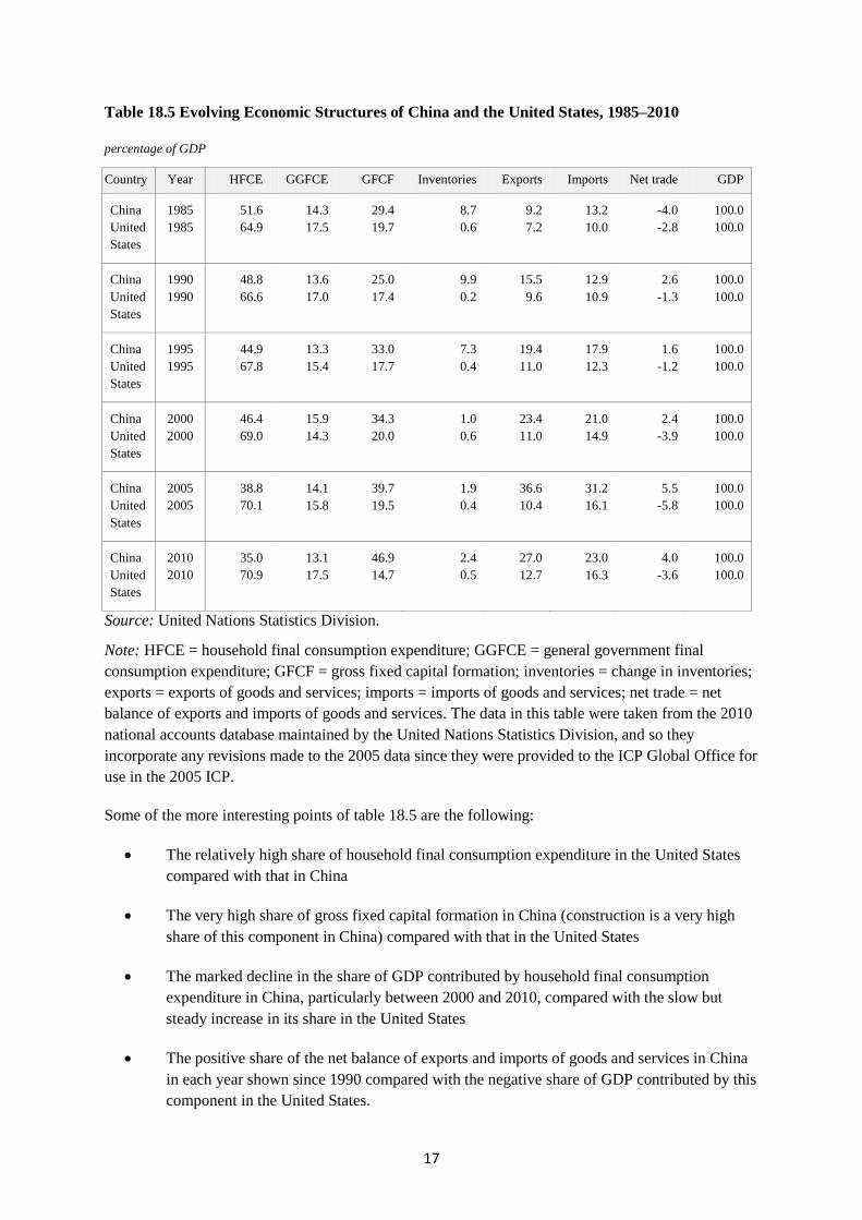
economic structures of China and the United States over the last few decades. Table 18.5 shows the
percentage of GDP contributed by each major expenditure aggregate for each fifth year from 1985 to
2010.
17
Table 18.5 Evolving Economic Structures of China and the United States, 1985–2010
percentage of GDP
Country Year HFCE GGFCE GFCF Inventories Exports Imports Net trade GDP
China 1985 51.6 14.3 29.4 8.7 9.2 13.2 -4.0 100.0
United
States
1985 64.9 17.5 19.7 0.6 7.2 10.0 -2.8 100.0
China 1990 48.8 13.6 25.0 9.9 15.5 12.9 2.6 100.0
United
States
1990 66.6 17.0 17.4 0.2 9.6 10.9 -1.3 100.0
China 1995 44.9 13.3 33.0 7.3 19.4 17.9 1.6 100.0
United
States
1995 67.8 15.4 17.7 0.4 11.0 12.3 -1.2 100.0
China 2000 46.4 15.9 34.3 1.0 23.4 21.0 2.4 100.0
United
States
2000 69.0 14.3 20.0 0.6 11.0 14.9 -3.9 100.0
China 2005 38.8 14.1 39.7 1.9 36.6 31.2 5.5 100.0
United
States
2005 70.1 15.8 19.5 0.4 10.4 16.1 -5.8 100.0
China 2010 35.0 13.1 46.9 2.4 27.0 23.0 4.0 100.0
United
States
2010 70.9 17.5 14.7 0.5 12.7 16.3 -3.6 100.0
Source: United Nations Statistics Division.
Note: HFCE = household final consumption expenditure; GGFCE = general government final
consumption expenditure; GFCF = gross fixed capital formation; inventories = change in inventories;
exports = exports of goods and services; imports = imports of goods and services; net trade = net
balance of exports and imports of goods and services. The data in this table were taken from the 2010
national accounts database maintained by the United Nations Statistics Division, and so they
incorporate any revisions made to the 2005 data since they were provided to the ICP Global Office for
use in the 2005 ICP.
Some of the more interesting points of table 18.5 are the following:
The relatively high share of household final consumption expenditure in the United States
compared with that in China
The very high share of gross fixed capital formation in China (construction is a very high
share of this component in China) compared with that in the United States
The marked decline in the share of GDP contributed by household final consumption
expenditure in China, particularly between 2000 and 2010, compared with the slow but
steady increase in its share in the United States
The positive share of the net balance of exports and imports of goods and services in China
in each year shown since 1990 compared with the negative share of GDP contributed by this
component in the United States.

18
The more fundamental issues, though, are that the structure of expenditure on GDP in China is in no
way similar to that of the United States in the periods shown, and the changes in shares over time are
in opposite directions in the major aggregates of household final consumption expenditure and gross
fixed capital formation. An important implication is that extrapolating (or backcasting) the 2005
Chinese PPP for GDP, which is the only one based on an actual data collection, is problematic when
the underlying assumptions of similarity in the structure and evolution between GDP in China and the
United States are taken into account.
One method used to backcast the real expenditures on GDP in China has been to take the real
expenditure on GDP from the 2005 ICP and then use the growth rates in China’s GDP volumes from
the time series national accounts to backcast that level, expressed in U.S. dollars for each year
involved (e.g., see Bhalla 2008). It is instructive to consider the unrealistic assumptions underlying
this process. Most critically, the relationship between the price level of GDP in China and in the
United States is assumed to be identical in every backcast year to that observed in the 2005 ICP. The
huge relative changes in the composition of GDP in the two countries shown in table 18.5 would
indicate that this critical assumption is unlikely to hold, particularly in view of the different PPPs
observed for individual components of GDP in China in 2005—see table 1, Purchasing Power
Parities, Local Currency Units per $US, in the report of the 2005 ICP (World Bank 2008).
Effects of Changes in the Terms of Trade
The ratio of the price of exports of goods and services to the price of imports of goods and services is
referred to as the terms of trade. The economies of many countries are often affected by large changes
in the terms of trade, particularly those countries that are major resource exporters, such as the oil-
producing countries, or commodity exporters, such as many countries in Sub-Saharan Africa. The
effects of any such changes are recorded, correctly, as part of GDP whether measured using the
expenditure, income, or production approach. For example, if the entire oil production is exported and
the price of oil doubles from 300 to 600 currency units from one year to the next while oil volumes
and every other aspect of the country’s economy remain the same, then the value of oil exports
doubles (an increase of 300), and so the value of expenditure on GDP increases by 300. The value of
mining production also increases by 300, and so the production-based GDP increases by 300. On the
income side of the national accounts, the operating surplus of the oil businesses increases by 300, and
so income-based GDP also increases by 300, thereby preserving the equality between the three
separate measures of GDP.
The expenditure-based estimates of GDP provide the values in the ICP, but a reference PPP
(exchange rates) is applied to exports and imports of goods and services. A sudden change in the
terms of trade does not affect a country’s exchange rate commensurately, and so the increase of 300 in
this example will be recorded largely as an increase in the real expenditure on GDP. On the other
hand, if the GDP deflator method is used to extrapolate a PPP and real expenditure benchmark, then
this increase in the value of exports is recorded as a price increase because there is no increase in the
volume of oil produced, leading to a mismatch between the extrapolated PPPs and those from a
benchmark.
The following method could be used to take account of this effect: extrapolate the net exports of
goods and services separately from the components of domestic final demand and adjust the rise in
export prices due to the oil price increase so that they will be more consistent with those obtained

19
from a benchmark comparison. Testing this process has shown that some significant gains can be
made in the accuracy of the extrapolated PPPs for some countries. However, it does not eliminate the
problem because the countries participating in the ICP have very diverse economies. In practice,
many different factors affect a country’s exports (and imports), and so the effects of changes in the
terms of trade are rarely sufficiently clear-cut to be attributable to a single cause such as an increase in
oil prices.
The Balassa-Samuelson Effect
In the early 1960s, Balassa (1964) and Samuelson (1964) independently hypothesized that price levels
in high-income countries are systematically higher than those in poorer ones. Decades later, Rogoff
(1996) found substantial empirical support for the Balassa-Samuelson effect, but in limited
circumstances. He found that the effect is most marked when very poor and very rich countries are
being compared, but it is generally less apparent when the comparison is between a group of relatively
rich countries. The development of the PWT provided new data that confirmed that the Balassa-
Samuelson effect did exist in practice. It also led to a related theory called the Penn effect.3 This effect
is based on the finding that expenditures on GDP adjusted to a common currency using market
exchange rates systematically understate PPP-based real expenditures on GDP for low-income
countries compared with high-income countries. In other words, the gap between GDP (and thus per
capita GDP) for high-income countries and low-income countries is exaggerated when market
exchange rates are used to adjust each country’s GDP into a common currency. Data from all the ICP
rounds to date have confirmed the Penn effect.
Ravallion (2010) describes the rationale for the Penn effect as follows:
In using the Balassa-Samuelson model to explain why PPPs tend to be lower (relative to market
exchange rates) in poorer countries, it is assumed that the more developed the country the
higher its labor productivity in traded goods, but that productivity for non-traded goods does
not vary systematically with level of development. A higher marginal product of labor in traded
goods production comes with a higher wage rate, which is also binding on the non-traded goods
sector (given that labor is freely mobile), implying a higher price of non-traded goods in more
developed countries and thus a higher overall price level. By the same reasoning, low real
wages in poor countries entail that non-traded goods tend to be cheaper. The ratio of the
purchasing power parity rate to the market exchange rate will thus be an increasing function of
income.
Using data from the 2005 ICP, Ravallion further developed the Penn effect by introducing what he
termed the dynamic Penn effect (DPE). The DPE describes the tendency for the gap between
exchange rate–based and PPP-based comparisons of GDP to narrow as the per capita real GDP for
low-income countries increases relative to that of high-income countries. The importance of the DPE
is that it may provide a means of adjusting extrapolated data so that they better match the next ICP
benchmark.
The data from the 2011 ICP will be important in terms of providing a firm benchmark to assess
whether taking account of the DPE in the extrapolated series leads to more accurate estimates than
those obtained using the current methods.
20
Differences between the 2005 and 2011 Benchmarks Caused by Changes in
Methodology
Extrapolating between benchmarks is also affected by changes in methodology between the two years
involved. The major methodological changes from the 2005 ICP to the 2011 ICP are the following:
Estimates of dwelling rents will be based on the quantity method instead of reference
volumes in the Asia-Pacific and African regions. However, the PPPs using the reference
volume method could be computed for 2011 so that the effect on the 2011 results of the
change to the quantity method can be computed.
The products priced in the global core list will have an impact on regional PPPs. Regional
PPPs can be computed with and without core items to determine their impact in 2011.
Using the important/less important classification (see chapter 7) will affect the 2011 PPPs.
In 2011 the PPPs, real expenditures, and price level indexes could be computed without
those classifications (as in the 2005 round) to determine the effect of using this
classification.
The global aggregation method proposed in 2011 will produce results that differ from those
obtained from the two-stage method used in 2005. The PPPs based on the method used in
2005 should be computed to determine the effect of this change in methodology.
In 2005 productivity adjustments were made in three of the six ICP regions (Africa, Asia-
Pacific, Western Asia), but the regional linking factors were computed without any
productivity adjustments. In the 2011 ICP round, it is likely that some regions will use
productivity adjustments, but others will not. However, linking factors across all regions
will be computed with productivity adjustments included for all regions.
The construction methodology is changing in the 2011 round, but it is so different from that
used in the 2005 round that it will be difficult to compare the effects of the change.
Once the 2011 results have been finalized, it will be possible to estimate the effects of most of the
methodological changes. However, it is important to emphasize that the differences estimated in this
way will provide indications of the effects of these changes rather than precise amounts.
Improving Extrapolation Methods
It is in the interests of all users of PPPs to have PPPs for non-benchmark years that are as accurate as
possible. It is clear that different methods will almost certainly lead to different results, and so it is
incumbent upon users to assess the implications of the underlying assumptions for their analysis. The
2005 ICP has provided an impetus to improve extrapolation methods, and a number of researchers are
investigating some promising alternative methods. The results of the 2011 ICP, which will be a firm
benchmark for virtually all the 146 countries that participated in the 2005 ICP, will provide
researchers with a much better data set than has been available to assess the reliability of the various
methods.

21
Possible means of improving methods for extrapolating PPPs include:
Extrapolating at the most detailed level possible rather than just for GDP. However,
experience has shown that lack of consistent, detailed price data will limit the possibilities.
Adjusting the price extrapolators for any terms of trade effect (e.g., by treating net trade
separately from the rest of GDP and using a domestic final demand deflator for this latter
component)
Systematically taking the dynamic Penn effect into account in the extrapolated PPPs, using
regression techniques to estimate the size of the effect.
In addition, several researchers (e.g., Hill 2004; Feenstra, Ma, and Rao 2009) are working on
completely new methods, such as econometric-based techniques, to provide more reliable time series
of PPPs and real expenditures.
Estimating PPPs for Nonparticipating Countries
Even though a record number of countries (146 in six regions) participated in the 2005 ICP, more than
50 countries did not take part. Many of these countries were in the lower-income group, which is the
main interest for many of those using the ICP results for poverty analysis. As a result, PPPs were
imputed for GDP for many of these countries using regression techniques, as done in earlier ICP
rounds. In the 2005 ICP, PPPs were imputed for 42 countries that had not participated in the program.
The method used was based on two explanatory variables in a logarithmic model to estimate GDP per
capita. The explanatory variables were (1) GNI per capita, expressed in U.S. dollars estimated using
the World Bank Atlas method; and (2) the secondary (school) gross enrollment rate.
A detailed description of the model used was provided in the global report for the 2005 ICP (World
Bank 2007), and the relevant parts are in annex C to this chapter.
Comparing ICP Benchmark Results
The results of the successive ICP rounds are independent of each other because they are expressed in
terms of the price levels prevailing in participating countries in each of the years involved. As for
comparing the results of two ICP rounds, it is useful to consider real expenditures and PLIs
separately, despite the close links between them.
Earlier, this chapter described the problems involved in maintaining consistency simultaneously
across time and space. Although these problems were in the context of extrapolating PPPs and real
expenditures from one ICP round to the next, they also have implications for comparisons of results
from successive ICP benchmarks. Directly comparing the ICP estimates of real expenditures for 2011
with those for 2005 should be carried out with the understanding that price levels not only changed
between 2005 and 2011 but also changed to a different extent across countries. Comparing the index
of per capita real expenditure on GDP for a country in two different years relative to a world (or
regional) average should be undertaken with the understanding that the structure of this average is
likely to have changed between ICP rounds and to varying extents, depending on the countries
22
involved. For example, a country with a large GDP and a higher than average growth rate in its
volumes will affect the world average real expenditure on GDP to a different extent in two successive
ICP rounds. The impact of such a country on a regional average will be even more pronounced. For
example, the total real expenditure in the Asia-Pacific region is dominated by China and, to a lesser
extent, India. Therefore, the economic behavior of these two countries will have a significant impact
on the average real expenditure for that region in each ICP round.
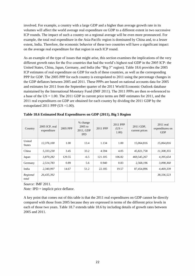
As an example of the type of issues that might arise, this section examines the implications of the very
different growth rates for the five countries that had the world’s highest real GDP in the 2005 ICP: the
United States, China, Japan, Germany, and India (the ―Big 5‖ region). Table 18.6 provides the 2005
ICP estimates of real expenditure on GDP for each of these countries, as well as the corresponding
PPP for GDP. The 2005 PPP for each country is extrapolated to 2011 using the percentage changes in
the GDP deflators between 2005 and 2011. These PPPs are based on national accounts data for 2005
and estimates for 2011 from the September quarter of the 2011 World Economic Outlook database
maintained by the International Monetary Fund (IMF 2011). The 2011 PPPs are then re-referenced to
a base of the US = 1.00. The 2011 GDP in current price terms are IMF estimates for 2011, and the
2011 real expenditures on GDP are obtained for each country by dividing the 2011 GDP by the
extrapolated 2011 PPP (US =1.00).
Table 18.6 Estimated Real Expenditures on GDP (2011), Big 5 Region
Country 2005 ICP, real
expenditure 2005 PPP
% change
2005 to
2011, GDP
IPD
2011 PPP
2011 PPP
(US =
1.00)
2011 GDP,
current prices
2011 real
expenditures on
GDP
United
States 12,376,100 1.00 13.4 1.134 1.00 15,064,816 15,064,816
China 5,333,230 3.45 33.2 4.594 4.05 45,821,758 11,308,355
Japan 3,870,282 129.55 -6.5 121.105 106.82 469,545,267 4,395,654
Germany 2,514,783 0.89 5.6 0.940 0.83 2,568,196 3,098,360
India 2,340,997 14.67 51.2 22.185 19.57 87,454,896 4,469,339
Regional
total
26,435,392 38,336,523
Source: IMF 2011.
Note: IPD = implicit price deflator.
A key point that comes out of this table is that the 2011 real expenditures on GDP cannot be directly
compared with those from 2005 because they are expressed in terms of the different price levels in
each of those two years. Table 18.7 extends table 18.6 by including details of growth rates between
2005 and 2011.

23
Table 18.7 Comparing Changes in Volumes and in Real Expenditures on GDP, Big 5 Region
Country
2005 ICP,
real
expenditure
on GDP
(1)
2011 real
expenditure
on GDP
(2)
2005 ICP,
index of
real expen-
diture on
GDP
(3)
Index of
2011 real
expen-
diture on
GDP
(4)
PPP-
implied
relative
growth
rate of real
expen-
diture (%)
(5)
2005 GDP
volume
(national
estimates,
local
currency)
(6)
2011 GDP
volume
(national
estimates,
local
currency)
(7)
% change
2005 to
2011
(GDP
volume)
(8)
National
accounts
relative
volume
growth
rate (%)
(9)
United
States 12,376,100 15,064,816 234 196 -16 12,622.95 13,287.89 5.3 -17
China 5,333,230 11,308,355 101 147 46 8,307.14 15,457.37 86.1 47
Japan 3,870,282 4,395,654 73 57 -22 536,762.20 537,356.11 0.1 -21
Germany 2,514,783 3,098,360 48 40 -15 2,220.95 2,428.52 9.3 -13
India 2,340,997 4,469,339 44 58 32 34,489.09 55,929.10 62.2 28
Sum 26,435,392 38,336,524
Average 5,287,078 7,667,305 100 100
Source: IMF 2011.
In table 18.7, the United States has an index of real expenditure on GDP of 234 (compared with the
Big 5 regional average of 100) in 2005, but this drops to 196 in 2011. The apparent implication is that
the U.S. economy contracted over this period, whereas in fact it grew by just over 5 percent. The
decline observed indicates that the U.S. economy grew significantly less than the regional average—
indeed, 16 percent less as shown in column (5) of table 18.7. Column (5) also shows that China and
India grew significantly more than the regional average (46 percent and 32 percent, respectively), and
that the United States, Japan, and Germany all grew less than the regional average. However, the level
of GDP was higher in the United States in both years than it was in China, although clearly the gap
between them narrowed. Column (9) of table 18.7 shows the GDP volume growth, relative to the
regional average, from the time series national accounts. The figures align very closely with the
relative changes in real expenditures on GDP in column (5). However, this alignment is a function of
the extrapolation methods used, and in practice the differences are likely to be much larger once the
2011 ICP results can be substituted for the extrapolated estimates in column (2) of this table. It is
important to note that the relative growth rates in real expenditures in columns (5) and (9) are not
proper temporal volume changes because they combine elements of both volume and price changes.
This example can be taken a step further by comparing each country’s share of the region’s total real
expenditure. The data in columns (1)–(4) in the following table have been taken from the
corresponding columns in table 18.7. Columns (5) and (6) show each country’s share of the regional
total in 2005 and 2011.

24
Table 18.8 Real Expenditures on GDP (Regional Average = 100), Big 5 Region
Country
2005 ICP, real
expenditure on
GDP
(1)
2011 real
expenditure on
GDP
(2)
2005 ICP,
index of real
expenditure
on GDP
(3)
Index of
2011 real
expenditure
on GDP
(4)
2005 real
expenditure
on GDP,
share of
regional
total (%)
(5)
2011 real
expenditure
on GDP,
share of
regional
total (%)
(6)
United
States 12,376,100 15,064,816
234 196 46.8 39.3
China 5,333,230 11,308,355 101 147 20.2 29.5
Japan 3,870,282 4,395,654 73 57 14.6 11.5
Germany 2,514,783 3,098,360 48 40 9.5 8.1
India 2,340,997 4,469,339 44 58 8.9 11.7
Regional
average
5,287,078 7,667,305 100 100 100.0 100.0
Source: IMF 2011.
In table 18.8, the index numbers for the United States, Japan, and Germany are all lower in 2011
(compared with the regional average) than they are in 2005, even though the GDP volumes in all three
countries rose between 2005 and 2011, albeit by only 0.1 percent in Japan (see column (8) of table
18.7). The reason for this is that the growth in GDP volumes in China (86.1 percent) and India (62.2
percent) between 2005 and 2011 resulted in a much higher share for each of these two countries in the
2011 regional total than that in 2005. Columns (5) and (6) of table 18.8 show the country shares of
real expenditure on GDP in 2005 and 2011, respectively. It is clear from these two columns that the
shares of China and India in the Big 5 region have increased significantly at the expense of the United
States, Japan, and Germany. As a result, to make sense of the changes in the indexes of real
expenditure on GDP between 2005 and 2011, it must be understood that the base (i.e., the regional
average) is different in each year, even though the indexes within each individual year provide useful
information. Comparing the changes in the shares of the regional totals between the two years helps
explain the changes in the indexes of real expenditure on GDP between 2005 and 2011.
One solution to this problem of the real expenditures being expressed in terms of different price levels
would be to adjust the values to take account of price changes between 2005 and 2011. However, the
results depend on the country chosen as the base country for the price level adjustments. In other
words, one set of results would be obtained if the price changes in the United States were used to
adjust the 2011 real expenditures to a 2005 price level. A different set of results would be obtained if,
for example, price changes in China were used to adjust the changes in real expenditures between the
two years.
Similar issues are encountered in attempting to interpret the PLIs between two successive ICP rounds.
PLIs are expressed in terms of a base—a country or, more commonly, a regional or world average.
The size of countries’ economies changes over time, as does the price level, and so the effect that any
individual country’s PLI has on the regional or world average changes between ICP rounds.
Therefore, the fact that a country’s PLI is higher (or lower) in one ICP round than in another does not

25
provide useful information in isolation. It needs to be interpreted in conjunction with other
information on the composition of the regional or world average on which it is based.
In summary, the ICP is designed to compare the real expenditures for countries within a year rather
than across years. However, it is possible to analyze the changes in real expenditure for a country
compared with the changes in real expenditure of a base country, or group of countries (i.e., the
relative changes). For example, assessing the relationship between pairs of countries is possible, such
as ―the real expenditure on GDP for country A was x percent higher than that for country B in 2011
compared with y percent higher in 2005.‖ The key point is that comparisons of the levels recorded in
2005 and 2011 between groups of countries (such as regional or world comparisons) will be more
problematic because of the different composition of the regional (world) average in the two years.
Rather than directly comparing the levels, it is necessary to take the extra step of estimating the
relative changes between the two years to explain the observed differences.

26
Conclusion
Collecting the data required to estimate PPPs and real expenditures is a time-consuming and costly
exercise. The first ICP, in 1967, produced data for a small number of countries, and the 2011 ICP
(with more than 180 participating countries) will be the eighth round overall. Therefore, an average of
more than six years separates each round. Because of increasing interest in international comparisons,
PPPs and real expenditures are required more frequently than once every six years, and so various
methods have been developed to produce annual estimates for the non-benchmark years. The different
methods do not produce the same results, nor will they necessarily match well with subsequent
benchmarks. In assessing the usefulness of the extrapolated PPPs and real expenditures, it is necessary
to understand the assumptions underlying the extrapolation procedures. This chapter is designed to
provide details about the various assumptions involved so that users can determine the method(s) that
best suit their circumstances. However, one critical point for users to consider is that experience has
shown that extrapolating PPPs and real expenditures will result in much more realistic data than the
alternative of using market exchange rates to convert values into a common currency.
Comparing the results from two ICP rounds is not a straightforward exercise because the real
expenditures for each year are expressed in terms of the (different) price levels for each of those
years. In interpreting the results from successive ICP rounds, it is necessary to note that the real
expenditures and price levels are expressed in relation to another country or to a regional average. As
a result, a decline in the relative position of one country within a region (or the world as a whole) does
not necessarily mean that the economic activity (or the price level) in the country concerned has
declined. Rather, it means that the economic activity (or the price level) in that country has increased
less rapidly than those in the other countries being compared.
Some of the improvements made for the ICP 2011 offer methods to more effectively extrapolate PPPs
in the future. For example, the set of core products used to link the regions could be used to obtain
some prices between benchmarks to estimate PPPs for aggregates below the GDP. Efforts to
harmonize CPIs across countries will also contribute to improved extrapolations.
This chapter closes with a note in annex D that provides an empirical analysis of the extrapolation
compared with a new benchmark. The analysis is based on Eurostat data for the household final
consumption expenditure (HFCE) aggregate in 17 European countries to show the divergence for a
number of six yearly extrapolations compared with the benchmark estimates. Note that the results
would be different if a more diverse range of countries were included or if the analysis were based on
GDP instead of on HFCE.

27
Annex A
World Bank Atlas Method
The following is an extract from 2010 World Development Indicators (World Bank 2010, 435).
In calculating GNI (gross national income) and GNI per capita in U.S. dollars for certain operational
purposes, the World Bank uses the Atlas conversion factor. The purpose of the Atlas conversion factor
is to reduce the impact of exchange rate fluctuations in the cross-country comparison of national
incomes.
The Atlas conversion factor for any year is the average of a country’s exchange rate (or alternative
conversion factor) for that year and its exchange rates for the two preceding years, adjusted for the
difference between the rate of inflation in the country and that in Japan, the United Kingdom, the
United States, and the euro area. A country’s inflation rate is measured by the change in its GDP
deflator.
The inflation rate for Japan, the United Kingdom, the United States, and the euro area, representing
international inflation, is measured by the change in the ―SDR deflator.‖ (Special drawing rights, or
SDRs, are the International Monetary Fund’s unit of account.) The SDR deflator is calculated as a
weighted average of these countries’ GDP deflators in SDR terms, the weights being the amount of
each country’s currency in one SDR unit. Weights vary over time because both the composition of the
SDR and the relative exchange rates for each currency change. The SDR deflator is calculated in SDR
terms first and then converted to U.S. dollars using the SDR to dollar Atlas conversion factor. The
Atlas conversion factor is then applied to a country’s GNI. The resulting GNI in U.S. dollars is
divided by the midyear population to derive GNI per capita.
When official exchange rates are deemed to be unreliable or unrepresentative of the effective
exchange rate during a period, an alternative estimate of the exchange rate is used in the Atlas formula
(see below).
The following formulas describe the calculation of the Atlas conversion factor for year t:
and the calculation of GNI per capita in U.S. dollars for year t:
Where
is the Atlas conversion factor (national currency to the U.S. dollar) for year t
is the average annual exchange rate (national currency to the U.S. dollar) for year t

28
is the GDP deflator for year t
is the SDR deflator in U.S. dollar terms for year t
is the Atlas GNI per capita in U.S. dollars in year t
is current GNI (local currency) for year t
is the midyear population for year t.
Alternative conversion factors
The World Bank systematically assesses the appropriateness of official exchange rates as conversion
factors. An alternative conversion factor is used when the official exchange rate is judged to diverge
by an exceptionally large margin from the rate effectively applied to domestic transactions of foreign
currencies and traded products. This applies to only a small number of countries, as shown in Primary
data documentation. Alternative conversion factors are used in the Atlas methodology and elsewhere
in World Development Indicators as single-year conversion factors.

29
Annex B
Transitivity of PPPs Extrapolated Using the GDP Deflator Method
In the 2005 ICP, the PPPs for all countries were transitive. Transitivity is an important condition in
the ICP because it ensures consistency in the results between any pair of countries, no matter whether
they are calculated directly between the two countries concerned or indirectly via a third country. For
example, in the 2005 ICP the transitivity condition for countries A, B, and C requires that
(18B.1)
where is the PPP for country A compared with country C in 2005.
The GDP deflator method used to extrapolate PPPs from a benchmark year to other years is described
in the section in this chapter that discusses the consistency between time and space. A useful
characteristic of this method is that the extrapolated PPPs are also transitive, and so no special
adjustments are required.
Extrapolating PPPs to year t using the GDP deflator method for countries A, B, and C results in the
following:
(18B.2)
(18B.3)
(18B.4)
where is the PPP for country A in year t;
is the implicit price deflator for GDP in country
A in year t (base 2005 = 100); and is the implicit price deflator for GDP in the United States in
year t (base 2005 = 100).
Using the relationships in (18B.2) and (18B.3), the PPP between countries A and B in year t is
(18B.5)
Similarly, from (18B.3) and (18B.4) the PPP between countries B and C in year t is
(18B.6)
and from (18B.2) and (18B.4) the PPP between countries A and C in year t is

30
(18B.7)
.
For transitivity to hold in the extrapolated series, one needs to show that
.
Based on (18B.7), this can be re-expressed in terms of the extrapolated series as
(18B.8)
).
Using the relationships in (18B.5) and (18B.6),
,
as required in (18B.8).
Therefore, the conclusion is that the PPPs in year t extrapolated from 2005 using the GDP deflator
method will be transitive in year t provided they were transitive in 2005.

31
Annex C
Estimation of PPPs for Nonbenchmark Economies
The following is an extract from Global Purchasing Power Parities and Real Expenditures: 2005
International Comparison Program (World Bank 2008, 164).
Each year, the World Bank includes estimates of PPPs for nonbenchmark economies in its World
Development Indicators publication and database, relying on an estimating equation using
information from the benchmark economies. The following estimating equation (5) was used to
impute values for missing economies from the previous round (1993–96) of the ICP:
Ln(GDP/cap) = 0.3402 + 0.5851*Ln(GNI/cap) + 0.2941*Ln(SGER) (5)
where:
GDP/cap is the ICP benchmark estimate of GDP per capita (PPP)
GNI/cap is gross national income (GNI) per capita in US$ estimated by the World Bank Atlas method
and SGER is the secondary (school) gross enrollment rate.
All three variables are indexed to the corresponding values for the United States (United States =
100). This model was first estimated using the benchmark results from earlier rounds and reestimated
when the 1993–96 results became available.
Using the preliminary results from ICP 2005, the model or equation (5) was reestimated to be model
or equation (6):
Ln(GDP/cap) = 0.3553 + 0.6994*Ln(GNI/cap) + 0.2292*Ln(SGER) (6)
The fit of the model might be improved by including additional independent variables correlated with
factor productivity and wage differentials because of imperfect labor mobility between economies and
between trading sectors and nontrading sectors. However, full exploration of various model
specifications is beyond the scope of this preliminary exercise, which is intended to replicate the
existing method so that other methods can be compared with it.
The above model is used to impute for nonbenchmark economies (the results are shown in table 8).
For a small number of economies whose Atlas GNI per capita of 2005 are not available, the model or
equation (6) is adjusted to replace GNI/cap with GDP per capita in US$ and is reestimated with all
available data in model or equation (7):
Ln(GDP/cap PPP) = 0.1987 + 0.7147*Ln(GDP/cap US$) + 0.2422*Ln(SGER) (7)
The input data and the reference GDP per capita in US$ are mainly taken from the World
Development Indicators database (April 2008).
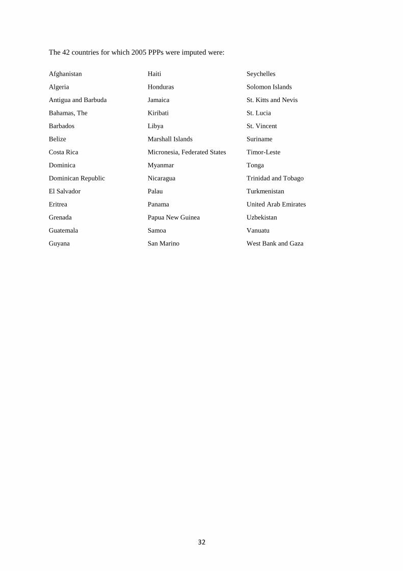
32
The 42 countries for which 2005 PPPs were imputed were:
Afghanistan Haiti Seychelles
Algeria Honduras Solomon Islands
Antigua and Barbuda Jamaica St. Kitts and Nevis
Bahamas, The Kiribati St. Lucia
Barbados Libya St. Vincent
Belize Marshall Islands Suriname
Costa Rica Micronesia, Federated States Timor-Leste
Dominica Myanmar Tonga
Dominican Republic Nicaragua Trinidad and Tobago
El Salvador Palau Turkmenistan
Eritrea Panama United Arab Emirates
Grenada Papua New Guinea Uzbekistan
Guatemala Samoa Vanuatu
Guyana San Marino West Bank and Gaza

33
Annex D
A Note on Extrapolating PPPs
Robert Inklaar and Marcel P. Timmer (University of Groningen)
Price level comparisons across countries are carried out infrequently, but there is a strong demand for
more frequent estimates. A common approach is to extrapolate the benchmark PPP using data on
price changes from the CPI or GDP implicit deflator. However, as this chapter makes clear, there are
conceptual and practical reasons why there will often be a mismatch between PPPs extrapolated from
a benchmark and the actual subsequent benchmark. To summarize, if the economic structure differs
between countries at either point in time, then extrapolating GDP PPPs using GDP deflators will lead
to a mismatch between the actual GDP PPPs and the extrapolated version, even if the price trends at
the detailed level are identical. In addition, there are many practical reasons why extrapolation leads
to different results than a subsequent benchmark. These include differences in price sampling,
weighting, and the omission of terms of trade in comparing GDP across countries.
In this note, we aim to provide some quantitative insight into this issue and distinguish between the
systematic and nonsystematic reasons extrapolation differs from actual benchmarks. This chapter lists
a range of systematic reasons: differences due to weighting (an index number problem), omitted
prices (e.g., terms of trade), revisions to time series but not to level comparisons, quality adjustment
of prices in some countries, and productivity adjustment of nonmarket services. In all these cases,
better data or measurement can remove these sources of differences. Nonsystematic differences are
harder to deal with—in particular, differences in the sampling frame (comparability over time or
across countries) and weighting below the basic heading level. At the basic heading level, these
differences will seem more like random error because solving them is highly problematic. Only if a
common data set of individual price quotes is used to estimate price changes over time and across
countries would we be able to eliminate these as a source of differences between extrapolated and
benchmark PPPs. However, even having such data sets would not completely eliminate such
differences in practice, although the data sets should reduce them significantly.
To quantify the importance of nonsystematic differences, we analyze a data set that does not suffer
from most of the systematic differences identified in this chapter, and then proceed to eliminate the
remaining systematic differences. For this purpose, we use Eurostat’s household final consumption
expenditure PPP and harmonized inflation data for 17 European countries (the old EU-15 plus Iceland
and Norway) for the period 1996–2010. By analyzing only HFCE, we find there are fewer systematic
differences because prices for exports, imports, and nonmarket services are not needed. By focusing
on these 17 countries, we presumably also minimize many nonsystematic differences because these
are all wealthy countries, and the recent period will also lessen any mismatch between methods used
for computing time series and cross-country relative prices.
Under Eurostat’s rolling benchmark approach, relative prices for one-third of the HFC products are
measured in a given year, and these are extrapolated using a detailed CPI series in the subsequent two
years. This way, there are annual observations for 146 HFC basic headings, and the HFC categories
can be matched to the detailed inflation series from Eurostat’s harmonized index of consumer prices
(HICP) data set.

34
To gauge the importance of systematic and nonsystematic differences in this data set, we use four
methods to compute the relative prices for the total HFC expenditure:
1. A GEKS aggregate of the 146 basic headings as given by Eurostat
2. A GEKS aggregate of the 146 basic headings, where the basic headings are extrapolated using
the most detailed inflation data available
3. A GEKS aggregate of the 146 basic headings, where the basic headings are extrapolated using
the aggregate inflation rate
4. An extrapolation of the overall HFC price level using the aggregate inflation rate (i.e., global
extrapolation).
To mimic the ICP situation, we extrapolated six years, using the 1996 price levels in combination
with inflation rates for the period 1996–2002. After six years, a new ICP benchmark would be
available to replace the last extrapolation. This means there are nine sets of extrapolated HFC price
levels to compare (1996–2002, 1997–2003, and so forth).
Method 1 is the same as that used by Eurostat, and the results correspond closely to the published
HFC price levels.4 Method 2 extrapolates basic heading prices in the same way as Eurostat, but
introduces no new benchmark information. The difference between results based on methods 1 and 2
is thus an indication of the importance of differences in sampling, methods of price collection,
definition of goods, and weighting below the basic heading level—that is, nonsystematic differences.
Method 3 omits price trends at the detailed level, but uses the same multilateral index number method
to compute relative prices. Comparing results based on this method to global extrapolation (method 4)
is the real-life counterpart to the stylized example of common price trends but different weights. The
difference in results between methods 2 and 4 can be seen as an upper bound to the index number
problem: both methods use the same price trends (HICP), but employ different weighting.
Table 18D.1 summarizes the comparison of the four methods.5 Columns (1), (2), and (3) compare
HFC price levels calculated using methods 2–4 to method 1, the official approach. Columns (4) and
(5) compare method 4 (global extrapolation) to methods 2 and 3. The results show that method 2
(extrapolating using detailed inflation rates and then aggregating) comes closer to the official results
than either of the other two methods. However, the differences are still notable at around 3 percent.
The results also show that methods 2, 3, and 4 are much closer to each other than to method 1. This
finding suggests that even in this data set, nonsystematic differences are the major source of
differences. It also shows that the index number problem—see column (4)—is modest in this context,
with a median difference of 1.4 percent. However, despite the nonsystematic differences being
quantitatively more important than systematic differences, table 18D.1 also shows that extrapolating
at a detailed level and then aggregating (method 2) leads to smaller differences with the eventual
benchmark than with global extrapolation (method 4). Evaluated at the median, the difference
decreases by about 20 percent (2.6 versus 3.3 percent).

35
Table 18D.1 Absolute Difference between HFC Price Levels, Methods 1 (pl1) to 4 (pl4)
percent
pl2/pl1
(1)
pl3/pl1
(2)
pl4/pl1
(3)
pl4/pl2
(4)
pl4/pl3
(5)
Mean 3.6 4.1 4.1 1.5 0.6
Median 2.6 3.1 3.3 1.4 0.5
25th percentile 1.3 1.4 1.8 0.7 0.2
75th percentile 5.2 5.7 6.0 2.1 0.8
Min 0.0 0.0 0.0 0.0 0.0
Max 12.0 16.2 14.3 5.4 2.9
Source:
Note: Summary statistics calculated across 144 observations: nine sets of price levels (1996–2002 to
2004–10) and 16 countries vis-à-vis Germany.
Conclusion
From this analysis, we have learned the following:
Extrapolated PPPs will in general not match a subsequent benchmark, even when accounting
for all systematic differences such as using the same weighting above the basic heading level.
Nonsystematic differences are more important for explaining the differences between
extrapolated PPPs and subsequent benchmarks. This finding may well be specific to the data
set of household final consumption expenditure in 17 European countries since 1996.
Removing systematic differences by extrapolating PPPs using prices at a detailed level and
aggregating using the same multilateral index number method as the original benchmark
brings the extrapolated PPPs closer to a subsequent benchmark than using global
extrapolation. In the current setting, the gain is comparatively modest (±20 percent), but in the
ICP setting all systematic differences are larger, so the gain should be larger as well.
Probably the only way to reduce nonsystematic differences would be to more extensively
draw on the same prices for international comparisons used for price indexes over time, such
as the CPI.
Fewer systematic differences arise in analyzing HFC than in analyzing GDP. The prices for
the other components of GDP are less firmly based than those for HFC, and so the likelihood
of inconsistencies between the prices provided by participating countries is higher. As a
result, conducting a similar analysis on GDP would almost certainly result in larger
differences than those observed for HFC.
36
References
Balassa, Bela. 1964. ―The Purchasing Power Parity Doctrine: A Reappraisal.‖ Journal of Political
Economy 72.
Bhalla, Surjit S. 2008. ―World Bank—Most Asians Dead in 1950.‖ Business Standard (India), August
23. http://www.business-standard.com/india/.
Biggeri, Luigi, and Tiziana Laureti. 2011. ―Understanding Changes in PPPs over Time: A Proposal
for the Extrapolation for Household Consumption Using CPI Data.‖ Paper prepared for the 6th ICP
Technical Advisory Group Meeting, Washington DC, October.
Commission of the European Communities, International Monetary Fund, Organisation for Economic
Co-operation and Development, United Nations, and World Bank. 2008. System of National Accounts
2008. http://unstats.un.org/unsd/nationalaccount/SNA2008.pdf.
Dalgaard, Esben, and Henrik Sejerbo Sørensen (Statistics Denmark). 2002. ―Consistency between
PPP Benchmarks and National Price and Volume Indices.‖ Paper prepared for the 27th General
Conference of the International Association for Research in Income and Wealth, Stockholm, August.
Eurostat and OECD (Organisation for Economic Co-operation and Development). 2006. Eurostat-
OECD Methodological Manual on Purchasing Power Parities. Paris: OECD.
Feenstra, Robert C., Hong Ma, and D. S. Prasada Rao. 2009. ―Consistent Comparisons of Real
Incomes across Time and Space.‖ Macroeconomic Dynamics 13 (Supplement 2): 169–93.
Hill, Robert J. 2004. ―Constructing Price Indexes across Space and Time: The Case of the European
Union.‖ American Economic Review 94 (5):1379–1410.
IMF (International Monetary Fund). 2011. World Economic Outlook Database.
http://www.imf.org/external/pubs/ft/weo/2011/02/weodata/index.aspx.
Khamis, S. H. 1977. ―Spatio-temporal Index Numbers.‖ Bulletin of the International Statistical
Institute 47 (4): 272–75.
Kravis, I. B., Z. Kenessey, A. W. Heston, and R. Summers. 1975. A System of International
Comparisons of Gross Product and Purchasing Power. Baltimore: Johns Hopkins University Press.
Ravallion, Martin. 2010. ―Price Levels and Economic Growth: Making Sense of the PPP Changes
between ICP Rounds.‖ Policy Research Working Paper 5229, World Bank, Washington, DC.
Rogoff, Kenneth. 1996. ―The Purchasing Power Parity Puzzle.‖ Journal of Economic Literature 34
(June): 647–68.
Samuelson, Paul. 1964. ―Theoretical Notes on Trade Problems.‖ Review of Economics and Statistics
46.
______. 1994. ―Facets of Balassa Samuelson Thirty Years Later.‖ Review of International Economics
2 (3).
Statistical Office of the United Nations and World Bank. 1982. World Product and Income:
International Comparisons of Real Gross Product. Washington, DC: World Bank.

37
World Bank. 2008. Global Purchasing Power Parities and Real Expenditures: 2005 International
Comparison Program. http://siteresources.worldbank.org/ICPINT/Resources/icp-final.pdf.
______. 2010. World Bank Indicators 2010. http://data.worldbank.org/data-catalog/world-
development-indicators/wdi-2010.
38
Notes
1. The rolling benchmark approach involves collecting prices for household final consumption expenditure
within a three-year cycle; about one-sixth of the prices are collected each half-year, and PPPs at the basic
heading level are extrapolated by price indexes that are specific to each basic heading. Prices for products in the
government final consumption expenditure and in gross fixed capital formation are collected more frequently.
2. Gross national income (GNI) is defined in the 2008 SNA as GDP plus compensation of employees receivable
from abroad plus property income receivable from abroad plus taxes less subsidies on production receivable
from abroad less compensation of employees payable abroad less property income payable abroad and less taxes
plus subsidies on production payable abroad.
3. This term was first used by Kravis et al. (1975) in referring to results in the 1970 ICP publication. The term
was coined because of the heavy involvement in that ICP round of Irving Kravis, Alan Heston, and Robert
Summers from the University of Pennsylvania. 4 There are some weighting differences because in later years more countries are included, but this has a
comparatively minor effect. 5 The detailed results confirm that the results from table 18D.1 are similar across countries and over the years.