1

Facility Fence Line Monitoring using Passive Samplers 1 2

3 Eben D. Thoma 4 U.S. EPA, Office of Research and Development, National Risk Management Research 5 Laboratory, 109 TW Alexander Drive, E343-02, Research Triangle Park , NC 27711, USA 6 7 Michael C. Miller and Kuenja C. Chung 8 U.S. EPA Region 6, 1445 Ross Avenue, Suite 1200, 6PD, Dallas, TX 75202, USA 9 10 11 Nicholas L. Parsons and Brenda C. Shine 12 U.S. EPA, Office of Air Quality Planning and Standards, 109 TW Alexander Drive, 13 E143-01, Research Triangle Park, NC 27711, USA, 14 15 16

ABSTRACT 17

In 2009, the U.S. EPA executed a year- long field study at a refinery in Corpus Christi, Texas, to 18

evaluate the use of passive diffusive sampling technology for assessing time-averaged benzene 19

concentrations at the facility fence line. The purpose of the study was to investigate the 20

implementation viability and performance of this type of monitoring in a real world setting as 21

part of U.S. EPA’s fence line measurement research program. The study utilized 14-day time-22

integrated Carbopack X samplers deployed at 18 locations on the fence line and at two nearby air 23

monitoring sites equipped with automated gas chromatographs. The average fence line benzene 24

concentration during the study was 1075 pptv with a standard deviation of 1935 pptv. For a six-25

month period during which wind direction was uniform, the mean concentration value for a 26

group of downwind sites exceeded the mean value of a similar upwind group by 1710 pptv. 27

Mean value differences for these groups were not statistically significant for the remaining six-28

month time period when wind directions were mixed. The passive sampling approach exhibited 29

acceptable performance with a data completeness value of 97.1% (n = 579). Benzene 30

concentration comparisons with auto gas chromatographs yielded an r2 value of 0.86 and slope of 31

0.90 with an approximately (n = 50). A linear regression of duplicate pairs yielded an r2 of 0.97, 32

unity slope, and zero intercept (n = 56). In addition to descriptions of technique performance and 33

general results, time series analyses are described, providing insight into the utility of two-week 34

sampling for source apportionment under differing meteorological conditions. The limitations of 35

the approach and recommendations for future measurement method development work are also 36

discussed. 37

2

38

IMPLICATIONS 39 Improved knowledge of air pollution concentrations at the industrial facility fence lines is a topic 40

of increasing environmental importance. Fence line and process monitoring can yield many 41

benefits ranging from enhanced risk management to cost savings through improved process 42

control. Efforts are underway within the U.S. EPA to develop and test a variety of cost effective 43

fence line monitoring strategies for potential use in a range of research and regulatory 44

applications. Among these, passive diffusive sampling is emerging as a promising technique for 45

time- integrated fence line monitoring applications. 46

47

INTRODUCTION 48

Development of cost effective and robust methods for detecting fugitive emissions and 49

monitoring air pollution concentration levels at industrial facility fence lines and remediation site 50

boundaries can yield many benefits. Implementable fence line and process monitoring systems 51

can enhance protection of public health and worker safety, advance emission inventory 52

knowledge, and realize cost savings by helping reduce product loss. A primary requirement for a 53

fence line monitoring system is that it provide adequate spatial coverage for determination of 54

representative pollutant concentrations at the boundary of the facility or operation. In an ideal 55

scenario, fence line monitors would be placed so that any fugitive plume originating within the 56

facility would have a high probability of intersecting one or more sensors, regardless of wind 57

direction. Sufficient measurement coverage can be accomplished using a small number of open-58

path instruments1-6 or through deployment of a larger number of point monitors. With either 59

approach, applications that require high detection sensitivity, chemical speciation, and fast time 60

response demand laboratory-class instrumentation which comes with significant capital and 61

operational cost. Currently, the expense of high performance, near real-time fence line 62

monitoring systems is likely perceived by industry to outweigh benefits. This is evidenced by 63

the lack of significant voluntary adoption causing potential benefits to go largely unrealized. 64

65

As part of U.S. EPA’s fugitive emission research program, a variety of cost effective fence line 66

and process monitoring approaches are under investigation with aim to improve understanding 67

3

and facilitate broader access to these technologies. Under the program, both time-resolved and 68

time- integrated measurement approaches are being explored. In long-term assessment or 69

screening applications where sensitivity and speciation are important but time response is not 70

critical, deployment of time- integrated passive diffusive samplers (PSs) with subsequent 71

laboratory analysis is a promising and cost-effective fence line monitoring approach. This paper 72

presents the results of a year- long field study using PSs to quantify fence line benzene 73

concentrations at a refinery in Corpus Christi, TX. The objectives of the study were to evaluate 74

the implementation feasibility, cost, and performance of the PS fence line monitoring approach 75

and to assess the effectiveness of time-integrated sampling for source apportionment under 76

varying meteorological conditions. 77

78

Flint Hills Resources collaborated with U.S. EPA in execution of this study by granting 79

permission to deploy the PSs and by allowing access to their on-site leak detection and repair 80

contractor for sample deployment. The study was performed at the Flint Hills West Refinery in 81

Corpus Christi, TX which has a nominal crude oil refining capacity of approximately 260,000 82

bbl/day. The West Refinery includes typical refining operations such as fluid catalytic cracking 83

and distillate hydrocracking, delayed coking, and associated petrochemical extraction and 84

conversion process units. For the study period, production was relatively consistent although 85

there were regularly scheduled maintenance and periodic shutdown and startup activities. Since 86

the emphasis for this study was on the use and performance of the PS measurement approach and 87

not on assessment of the actual emissions from the refinery, no attempt was made to gather 88

detailed process or operation information. Due to the relative consistency of production 89

throughout the year and the time- integrated nature of the measurement, it is believed that day to 90

day production variability had little impact on observations or the data groupings suggested 91

below. 92

93

EXPERIMENTAL METHODS 94

The use of PSs with a variety of designs and sorbent materials for ambient monitoring 95

applications has been documented in the literature7-13 with much effort related to the 96

development of monitoring protocols for the European Community Directive 2000/69/EC and 97

daughter directives that set limits on ambient concentrations of hazardous air pollutants including 98

4

benzene. The current study utilized Carbopack X sorbent (≈ 650 mg) in ceramic- lined Perkin-99

Elmer (PE) tubes (Supelco, Inc., Bellefonte, PA), 6 mm in dia. by 90 mm length, with laboratory 100

analysis by thermal desorption gas chromatograph (TurboMatrix ATD, PerkinElmer Instruments 101

LLC, Shelton, CT and Saturn 2000 GC/MS, Agilent, Santa Clara, CA). Information on use of 102

Carbopack X sorbent for determination of the concentration of benzene and other volatile 103

organic compounds in ambient air14-17 along with details on the custom Carbopack X PE tubes 104

and laboratory analytical procedures used in this study are summarized by McClenny, Mukerjee, 105

and others.16-19 106

107

For this study, a two-week PS deployment schedule was utilized. Each PS was exposed to 108

ambient air for a 14-day period (P) and then replaced with an unexposed PS. A total of 26 PS 109

sets, designated P1through P26, were deployed from December 3, 2008, to December 2, 2009. 110

The PS set change was executed between 8:00 a.m. and 11:30 a.m. and required approximately 111

1.5 hours to complete with additional time for record keeping and shipping to the laboratory for 112

analysis. For cost efficiency, samples were analyzed and samplers were reconditioned for 113

redeployment in batches requiring multiple sets of PSs to be used to prevent sampling 114

discontinuity. The PSs were covered with a rain shield and attached to the boundary fence of the 115

facility at approximately 1.5 m above the ground. The samplers were changed by the facility 116

leak detection and repair (LDAR) contractors who were trained by EPA representatives in proper 117

procedures prior to the study. Additional information on study execution can be found in the 118

quality assurance project plan.20 119

120

The PSs were deployed at 18 locations on the fence line of the Flint Hills Refinery West Facility 121

in Corpus Christi, TX, and at two Texas Commission on Environmental Quality (TCEQ) 122

continuous air monitoring station (CAMS) sites: C633, south of the facility (Fig. 1); and C634, 123

located approximately 10 km east of the facility (not shown). The PS locations (loc) are labeled 124

by their approximate angular position as observed from the center of the facility with north 125

representing zero degrees. The configurations of the PSs were fixed for the study with the 126

exception of loc 40, 50I, and 60 which were added during P12 to help diagnose high observed 127

concentrations in the vicinity of loc 50. Duplicate and field blanks were deployed at loc 180 and 128

C633, with duplicates added to loc 360 during P22. TCEQ CAMS sites C633 and C634 129

5

performed automated gas chromatograph (GC) benzene measurements providing one hour 130

average concentration values (Clarus Model 500 GC, Perkin-Elmer, Waltham, MA) and PSs 131

were placed at both locations for comparison purposes. Also shown in Figure 1 are TCEQ 132

CAMS sites C631 and C632, which did not operate auto GCs but provided total nonmethane 133

organic carbon (TNMOC) measurements and meteorological data useful for future comparisons. 134

135

The PS data set produced by the year- long deployment consisted of 579 samples, including 56 136

duplicates and 49 field blanks. Seventeen samples were excluded from the analysis due to 137

combination of tube damage or deployment issues (n = 6) and laboratory equipment malfunction 138

(n = 11), yielding a data completeness value of 97.1%. The benzene concentration data for 10 139

samples exceeded the demonstrated linearity range of 4071 pptv for the analytical system 140

utilized and, as a consequence, these values contain additional uncertainty estimated to be below 141

20%. Further information on the PS configuration, deployment, and laboratory analysis can be 142

found in the quality assurance project plan and supplemental information.20 143

144

RESULTS AND DISCUSSION 145

The objective of this study was to gain information on the implementation feasibility and 146

measurement performance of the two-week passive samplers in a real-world fence line 147

deployment scenario. Information such as overall data completeness, duplicate and field blank 148

data, site to site trend consistency, and comparisons with automated gas chromatographs help 149

form a basis for judging the efficacy of the overall measurement approach. The results section 150

begins with a description of meteorological conditions encountered during the study and PSs 151

validation data. An overview of the combined fence line results by location and period are then 152

presented. This information is followed by a discussion of time series results and upwind vs. 153

downwind comparisons under uniform and mixed wind direction conditions. The latter data is 154

important because it provides valuable insights on the general utility of time-integrated 155

monitoring for determining a facility’s contribution to the observed fence line concentrations. 156

157

Meteorology 158

The 14-day average of hourly wind direction (WD), scalar wind speed (SWS), vector resultant 159

wind speed (RWS), temperature (T), and relative humidity (RH) data recorded by the C633 160

6

site21 are summarized in Table 1. The SWS represents a simple average of hourly values of wind 161

speed for the two-week period. The RWS was determined by first calculating the orthogonal 162

vector components (north = 0 °, east =90°) for each hourly reading, averaging individual 163

components for the period, then calculating the magnitude of the resulting vector. The RWS 164

increases from zero with decreasing WD variability, approaching the value of SWS when winds 165

are highly uniform over the two week period. The difference in RWS and SWS is one of several 166

ways to quantify the degree of wind direction uniformity which is important for time- integrated 167

sampling approaches. Confidence in meteorological data acquired from the TCEQ CAMS site is 168

bolstered by State’s quality assurance requirements and additionally by well-correlated cross 169

checks with nearby CAMS sites for important meteorological variables. 170

171

In comparison to other parts of the U.S., Corpus Christi exhibits strong wind speeds and periods 172

of highly uniform wind direction which can have a significant effect on comparative analysis 173

with time- integrated monitors. In preparation for discussion on this point, two six-month 174

groupings of wind data from the study are presented in Figure 2. Figure 2a shows a wind rose 175

for a grouping of P1-P6 coupled with P20-P26 and reflects a period of relatively mixed wind 176

directions. Figure 2b shows a grouping of P7-P19 exhibiting a continuous six month period 177

when the wind direction was more uniformly from the southeast. For the grouping of Fig. 2a, the 178

average difference in SWS minus RWS is 7.0 mph, whereas for the more uniform case the 179

difference is 2.8 mph. A six month grouping of neighboring periods was chosen for simplicity 180

with period cut-off decided by comparing the SWS and RWS values for individual periods. 181

182

PS Validation Results 183

Benzene concentration data determined by PSs were compared to the 14-day average of 1 hour 184

data from the GCs at the C633 and C634 sites. A linear regression of PS and GC data (Figure 3) 185

shows an unconstrained r2 value of 0.86 and slope of 0.90 (n = 50 using average values for 26 186

duplicate pairs at C633). The Method Detection Limit (MDL) for the PS was determined to be 187

35 pptv and the MDL for the GC was found by TCEQ to be 50 pptv for benzene for the study 188

period. Figure 3 utilizes all reported GC data which includes a significant number of hourly 189

values below the MDL (25%) with a disproportionate number occurring in the P7-P19 periods 190

with winds away from the facility. As an example, for P14-P19, only 1036 of a possible 3427 191

7

GC values were above the MDL. For the same time period, the average value of the PS 192

concentrations at the GC locations was 139 pptv with a minimum of 85 pptv, significantly above 193

the MDL, owing to the time-integrated nature of the sampling approach. The y- intercept value 194

of 142.2 pptv in Figure 3 is largely determined by the decision to include all available GC data in 195

the comparison. Removing all GC data below the MDL gives a linear regression r2 value of 196

0.78, a slope of 0.87 and a y- intercept of 91.85 pptv. These data comparisons ultimately depend 197

on the definition of Minimum Quantization Limit (MQL) and the choice for assignment of fixed 198

values for below MQL entries. This highlights a difficulty in comparing time- integrated and 199

time-resolved approaches which is not of major concern for current discussion on fence line 200

monitoring where levels significantly above MDL are of primary importance. 201

202

The range of comparison for the PS and GC data (≈100 pptv to ≈1000 pptv) is somewhat lower 203

than optimal for validation purposes. The low upper limit on two-week average concentrations 204

at the TCEQ sites was due in part to their locations that were significantly displaced from the 205

fence line of the facility. While not optimal, the upper limits of comparison are reasonable when 206

considering the overall PS study average for fence line locations was ≈1000 pptv. To achieve 207

higher ranges of comparison, future field studies should consider co-deployment of PS and GC 208

on the fence line of facility near areas of high expected concentration. In addition to Figure 3, 209

time series comparisons of C633 GC and C633 PS providing further validation information are 210

discussed in a subsequent section. 211

212

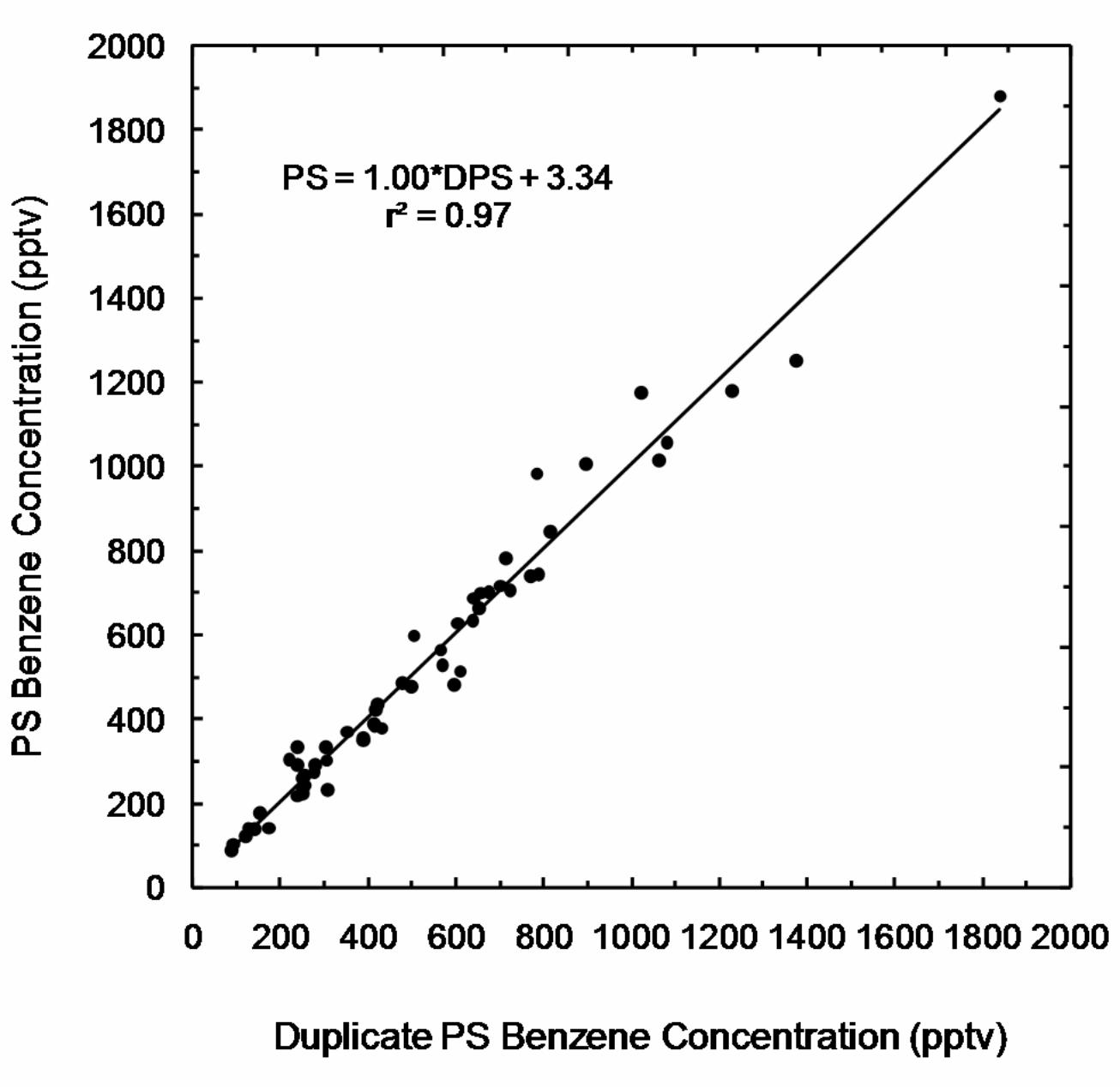
Duplicate PSs were located at C633 and loc 180 for all periods, and at loc 360 for P22 through 213

P26 (Figure 4). Concentrations of duplicate pairs ranged from approximately 100 pptv to 1200 214

pptv with a linear regression r2 = 0.97, unity slope, and near zero intercept, n = 56. The average 215

difference in the duplicate values was 8.5% with a maximum of 33% occurring for a low range 216

reading (229 pptv vs. 333 pptv). Duplicates were added to loc 360 during P22 in response to 217

high readings observed in P14 and P15. The delay in deployment of the duplicates was due to 218

the batch processing of samples, which delayed data availability. Field blanks deployed at loc 219

180 and C633 had an average value of 8.0 pptv with a standard deviation of 6.2 pptv, n = 49. 220

Supplemental table S1 contains all duplicate, GC, and field blank data for the study.20 221

222

8

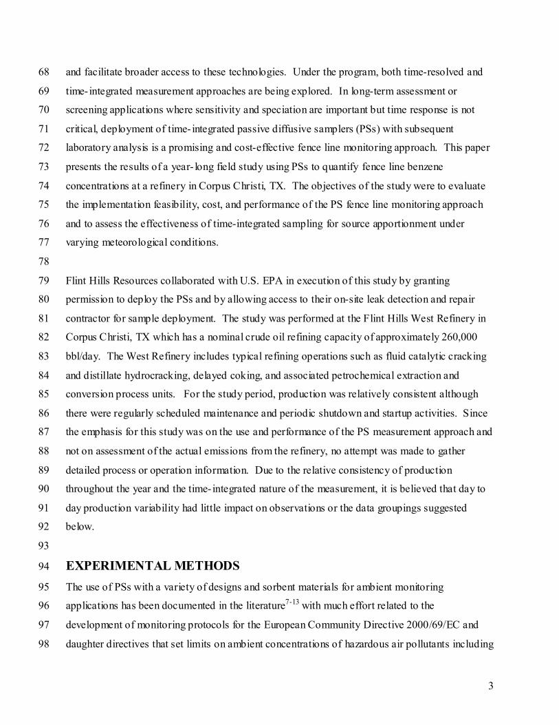
PS Fence Line Results 223

A total of 454 PSs were deployed at 18 fence line sites around the facility (Fig. 1). Combining 224

all fence line PS results, the mean benzene concentration was 1075 pptv with a standard 225

deviation (s) of 1935 pptv. The PS median value was 709 pptv with a minimum of 122 pptv and 226

a maximum of 29280 pptv. With fence line-deployed duplicates averaged, 8.5% of readings 227

were above 2000 pptv, 21.2% were between 1000 and 2000 pptv, and 70.3% were below 1000 228

pptv. Fence line PS data, along with the off-site C633 PS data, are summarized by location in 229

Figure 5. The C633 PS has a mean benzene concentration value of 318 (s = 160) pptv, slightly 230

below neighboring fence line sites, loc 250 (≈ 630 m away) with a mean value of 416 (s = 183) 231

pptv, and loc 270 (≈ 510 m away) with a mean value of 395 (s = 121) pptv. The differences in 232

the means of C633 compared with loc 250 and separately with loc 270 are statistically significant 233

at alpha = 0.05 with t-test p-values of 0.042 and 0.048, respectively. The ability to detect 234

differences in PSs deployed on the fence line and at proximate off- site locations is potentially 235

important in future gradient-based source comparison strategies. 236

237

PS benzene concentration values on the predominately upwind southern fence line, consisting of 238

loc 130 through loc 250, show a group mean of 613 (s = 353) pptv, lower than the northern 239

fence line (loc 310 through loc 50) having a group mean of 1840 (s = 3169) pptv with group 240

mean difference p-value < 0.001. Excluding the two extreme outliers at loc 360, the northern 241

fence line group mean is 1512 (s = 1494) pptv with similar group mean difference p-values. 242

243

Figure 6 shows PS benzene concentration data for a subset of fence line locations by sampling 244

period (loc 40, 50I, and 60 are not included due to incomplete sets). The mean values and 245

number of outliers (values that extend beyond 1.5 times interquartile range) are somewhat higher 246

in the warmer months and lower in the cooler months. It is not known if these differences are 247

due to higher emissions or to the effects of atmospheric conditions on ground level 248

concentrations at different times of the year. Since PSs comparisons with auto GC show little 249

seasonal variation (next section), these differences are not believed to be due to measurement 250

bias. 251

252

9

As discussed in the text associated with Figure 2, it can be informative to form two six-month 253

groupings of PS results from neighboring time periods. This is performed here with the spatially 254

integrated data of Figure 6 and in a subsequent section by resolving the locations into upwind 255

and downwind subgroups. The mixed wind direction six-month group (Fig. 2a) contains cooler 256

months (average T = 68° F) and has a mean benzene concentration value of 798 (s = 414) pptv, n 257

= 188. The uniform wind direction grouping (Fig. 2b) has a higher average temperature (T = 80° 258

F) and a mean concentration value of 1288 (s = 2799) pptv, n = 192. There is a statistically 259

significant difference in group means (p = 0.017) for these sets. For this data comparison, 88.5% 260

of readings above 2000 pptv occur in the P7-P19 uniform wind group. These observed 261

differences were not due to changes in refinery operations as production levels were confirmed 262

to be relatively consistent throughout the study period. 263

264

Time Series Comparisons 265

Techniques for temporal analysis of fence line monitoring data are determined in large part by 266

the time resolution of the measurement. For example, monitoring schemes with time resolutions 267

less than one hour can utilize intra-day trend analysis and metrological comparisons to help 268

apportion local source contributions. The time- integrated nature of the PS approach makes it 269

less useful in this context; however, important information on longer-term temporal and spatial 270

trends can be gained through time series comparisons. Since the implementation cost of the PS 271

approach is lower than similar density deployments of time-resolved monitors, passive sampling 272

has clear advantages for acquisition on longer-term trend information. 273

274

Figure 7 examines the southern fence line benzene concentrations from the C633 auto GC, the 275

collocated C633 PS, and the average of two nearby sites, loc 250 and loc 270. Similar trends in 276

the concentrations are evident. For example, comparatively lower concentrations in P7 and P9 277

through P19 are observed for both the PS and auto GC even though the overall average 278

concentration for the fence line sites is higher for these periods (Fig. 6). Basic wind direction 279

expressed as the percentage of winds coming out of the southern hemisphere is shown on the 280

secondary y-axis. During periods P7, P11, and P14-P20, winds are directionally towards the 281

north, transporting facility source signal away the from the southern fence line samplers, 282

resulting in lower observed concentrations. A linear regression comparison of C633 PS data 283

10

with a percentage of southerly winds yields an unconstrained r2 value of 0.87. This relatively 284

high correlation indicates that the PS readings are likely influenced by emissions transported 285

from the facility and also that the two-week time- integrated sampling approach is able to register 286

changes in prevailing wind orientation with respect to the source. 287

288

The similarity in the time series for the fence line PS (loc 250 and loc 270) and the offsite PS 289

(C633) provides some confidence that the mobile sources using Interstate Highway 37, located 290

between the observation points (Fig. 1), are not producing significant interfering benzene signal. 291

If this were the case, divergence in the time series with changing prevailing winds would be 292

expected. The time series shown in Figure 7 also provides supporting validation information for 293

the PS by showing similar period-to-period variations of the PS compared to the auto GC. 294

Similar comparative results were also observed for the C634 site. These comparisons, taken over 295

the year- long study, provide some evidence that seasonal changes in temperature and humidity 296

have little effect in PS performance for the range of conditions encountered in this field 297

campaign. 298

299

Ideally, the fence line PSs should be deployed away from obstructions which can impede wind 300

flow and also away from potential interfering sources outside of the fence line. Both of these 301

situations can lead to elevated concentrations measured by the PS that are not due to the 302

observed facility. Time series analysis along with deployment of additional diagnostic samplers 303

can be used to help understand elevated PS readings and to identify PS siting and interfering 304

source issues. Figure 8 shows PS benzene concentrations in the neighborhood of loc 50 (Fig 1.), 305

which is positioned in a complicated environment including complex local topography and 306

potential neighboring sources. The ground level to the southwest, near loc 50I, is elevated by 307

approximately 2 m compared to the location of loc 50. This local topography could cause 308

complex wind flow (channeling or vortices) in the neighborhood of loc 50 potentially affecting 309

measured concentrations. Potential sources such as the barge loading operations to the north and 310

the wastewater treatment to the southeast are outside the defined fence line. Location 50 311

exhibited the first notably high concentration during P7 and, in response to this reading, several 312

additional PS sites were implemented (loc 40, 50I, and 60) during P12. These samplers also 313

showed somewhat elevated concentrations prior to P20, but the results are difficult to correlate 314

11

with loc 50 values or wind direction. For this fence line location, the combination of topography 315

and additional potential sources makes it difficult to draw conclusions about emissions from the 316

primary observed target, the facility to the southwest. For example, the PS at loc 50I is inside 317

the fence line, closer to the potential facility sources (tanks). Due to proximity, we would expect 318

higher concentrations at loc 50I compared to loc 50 if the primary source were the observed 319

facility, all other factors being equal. Additionally, the three highest readings at loc 50 occur 320

during P7, P11, and P16 with a high percentage of winds from the south (Fig. 7) and more 321

specifically from the southeast (Fig 2b). This fact, coupled with the relative response of 322

neighboring PSs, implies that the wastewater treatment area outside the defined fence line is a 323

likely interfering source. 324

325

A strength of PS-based fence line monitoring is in providing cost-effective, high spatial density 326

long-term monitoring capability. As evidenced by the results of Figure 8, a weakness of time-327

integrated monitoring lies in its inability to apportion contributions to the measured 328

concentration in complex source and micrometeorological conditions. In cases where additional 329

source apportionment capability is required, the PS approach can be selectively augmented 330

through the use of time-resolved fence line monitoring coupled with wind direction analysis. 331

332

The time series of Figure 9 illustrates the elevated nature of data acquired downwind of the 333

facility and also provides some perspective on extreme outlier readings. In comparison to 334

upwind site loc 130, the downwind sites register consistently higher benzene concentrations, 335

especially during P7-P19 where winds are uniformly from the southeast. The two highest 336

readings were recorded at loc 360 during P14 and P15 (29,280 pptv and 20,007 pptv, 337

respectively). These outlier values are significantly elevated compared to the third highest 338

reading of 8891 pptv (loc 20, P11) and are ≈ 6 standard deviations displaced from the northern 339

fence line group average of 1840 pptv. At approximately 5 times the demonstrated analytical 340

linearity range for this study, the accuracy of the P14 and P15 outlier readings is uncertain. 341

However, the occurrence of significantly elevated values at loc 360 during these periods is not 342

unexpected when considering the elevated neighboring observations in the time series of Figures 343

8 and 9. 344

345

12

Two-week integrated PS readings at the 30,000 pptv level are somewhat difficult to understand 346

since if these readings are not due to gross analytical error, they are a result of either sustained 347

elevated concentrations transported by the wind to the sampling location or a shorter time 348

duration intense spike in local concentration in close proximity to the PS caused by a transient 349

source. Since the two similar outlier values were produced from separate sorbent tubes and 350

analyzed during different laboratory runs, it is unlikely that analytical error is the cause of the 351

elevated readings. The explanation of sustained elevated benzene concentrations at the PS is 352

somewhat unlikely considering loc 360 is over 300 m distant from the nearest above-ground 353

facility structure (tanks to the south east, Fig. 1). These observations do not preclude the 354

presence of a below-ground emission or a temporary source not obviously part of the facility 355

fence line observation. An unknown or temporary source, such as a rail car, could have been 356

located in very close proximity to the loc 360 PS thereby causing a large integrated response. 357

358

A local benzene spike could include an actual emission or could be attributed to a sample 359

handling issue. As an example of the latter, the field operators were instructed not to refuel their 360

vehicles prior to sample handling to reduce the chance that gasoline vapor entrained on their 361

hands could provide an intense concentration spike to the PS when uncapped during deployment. 362

This type of sample corruption could affect two successive sampling periods as both the pick-up 363

of the deployed PS and the placement of the new PS occur at similar times. This type of 364

deployment error can be investigated by looking at neighboring samples (loc 20 and loc 330), 365

which in this case were deployed within seven minutes before and after the loc 360 P15 PS and 366

did not show abnormally high results. In future PS protocol development work, placement of 367

secondary samplers with offset deployment schedules could assist in diagnosing outlier issues. 368

These secondary samplers could be analyzed only when abnormal results arise to minimize cost 369

for this diagnostic. 370

371

Upwind vs. Downwind Comparisons 372

A primary objective of any fence line monitoring strategy is to positively identify the observed 373

facility’s contribution to the measured concentrations. One way to accomplish this is by 374

comparing the concentrations registered by the monitors stationed upwind (UW) of the facility 375

with downwind (DW) sampling locations with the difference indicative of emissions. Since 376

13

meteorological conditions change over time, the designation of UW and DW monitors is 377

mutable. When using time-resolved fence line monitoring instrumentation, this UW vs. DW 378

comparison is accomplished by reviewing measured concentration data in conjunction with 379

simultaneously acquired meteorological data. When using two-week time integrated PSs, this 380

approach is less viable, especially in cases where the wind direction is mixed. 381

382

To investigate this effect, we can compare uniform and mixed wind direction scenarios by using 383

the two six month periods defined in Figure 2. An UW group, consisting primarily of southern 384

fence line sites (loc 90 through loc 270), and a DW group (loc 290 through loc 20) can be formed 385

for both the P1-P6, P20-P26 mixed wind direction case (Fig. 2a) and the P7-P19 uniform wind 386

direction case (Fig. 2b.) For the mixed wind direction case, the UW mean is 768 (s = 366) pptv 387

and the DW mean is 718 (s = 297) pptv [Fig 10(a)]. Differences in these group means are not 388

statistically significant (p-value = 0.330). For the uniform wind direction case, the UW mean of 389

487 (s = 277) pptv is significantly lower than the DW mean, 2197 (s = 4361) pptv with a p-value 390

= 0.003 [Fig 10(b)]. Excluding the two high outliers at loc 360, the DW mean becomes 1473 (s 391

= 1371) pptv with an improved p-value of <0.001 for a mean difference comparison with the 392

UW samples. Comparing across the mixed and uniform wind direction cases, the UW means are 393

also statistically different from each other at the 99% CI. For multi-month groupings of two-394

week PSs, it is possible to resolve UW and DW differences in the case of highly uniform wind 395

direction. However, it is difficult to draw conclusions on facility contributions to the measured 396

fence line concentrations using a simple UW-DW approach for the mixed wind direction case 397

that may be more typically encountered in other areas of the U.S. 398

399

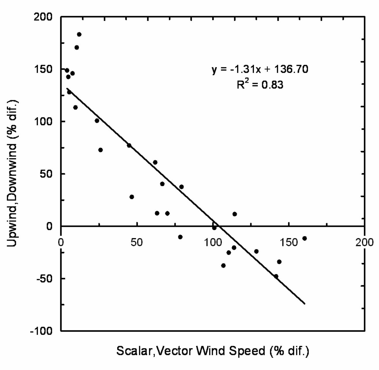
To further investigate the effects of wind direction, Figure 11 plots the percentage difference in 400

UW and DW benzene concentrations with a metric indicative of wind direction uniformity 401

formed by calculating the percentage difference in the scalar and resultant vector wind speeds 402

(SWS and RWS in Table 1). For periods with uniform wind direction, SWS and RWS are 403

similar, so emissions from the facility are transported toward the DW sampling locations a high 404

percentage of the time, resulting in a larger difference in the UW and DW concentrations. As the 405

difference in SWS and RWS increases, the temporal overlap of the facility-generated plume is 406

more equally shared between the UW and DW samplers, so their percentage difference decreases 407

14

and actually becomes slightly negative during the winter months as the UW leg experiences 408

higher concentration on average. The relationship expressed in Figure 11 depends on the 409

definition of UW and DW sites which may change throughout the year based on site-specific 410

metrological conditions. 411

412

The ability to resolve statistically significant differences in PS concentrations using fence line 413

deployed PSs depends on the degree of wind direction uniformity and also on factors such as 414

sampling time integration, wind speed (degree of stagnation), and on the offset distance of PS 415

from facility sources (dilution effects). At 14 days, the time duration of sampling used for this 416

study was judged to be an optimal trade-off between time resolution and cost. To help increase 417

the diagnostic capability of the two-week PS approach, future protocol development could 418

include a significant number of off- fence line sites set back from the primary monitors so as to 419

allow concentration gradient analysis to aid in deciphering facility contributions under mixed 420

wind direction cases. The reduction in concentration by atmospheric dispersion along the 421

gradient will help provide source apportionment information. Additionally, ways to 422

systematically define UW and DW site groups based on statistical comparisons of concentrations 423

on a rotating sector basis should be explored. 424

425

CONCLUSIONS 426

This field demonstration provides first- level validation data for the PS fence line monitoring 427

approach while informing future method development needs. With high data completeness rates, 428

the year- long study provides evidence that the approach is relatively robust and implementable 429

by modestly trained personnel. Based on cost figures from the current study, the expense for 430

commercial application of a standardized method is projected to be below $200 per sample for a 431

single component analysis. The implementation factors for the PS approach are attractive in 432

comparison to similar density deployments of time-resolved monitoring technologies which can 433

come at much higher capital and operational costs. 434

435

The PS fence line concept can provide useful information on overall concentration levels and 436

potential problem areas on the facility fence line using simple source identification techniques 437

such as upwind-downwind comparisons, temporal trend investigation, and gradient analysis. A 438

15

weakness of the time-integrated approach is found when attempting source apportionment in 439

complex environments. In this event, elevated concentration areas found in the PS screen can be 440

further investigated with selective use of time-resolved monitoring where deemed necessary. 441

The use of PS alone or in combination with optimally deployed time-resolved monitors can form 442

the basis for cost effective and flexible fence line monitoring strategies. 443

444

Remaining method development questions center on establishment of PS performance with a 445

wider concentration range and the expansion to compounds other than benzene. Future 446

validation work should consider GC placement at downwind fence line locations to expand the 447

range of comparison and potentially include the deployment of spikes duplicate samples to 448

investigate out gassing effects. New deployment strategies must also be developed to allow 449

effective source apportionment for the observed facility in areas with mixed wind directions and 450

higher percentages of stagnant conditions. These deployment strategies are envisioned to 451

include a gradient sampling approach with PS monitors placed progressive distances from the 452

fence line. Another area for improvement is optimized duplicate deployment strategies to 453

provide additional quality assurance information in the event of anomalous primary readings. 454

For cases of complex sources or joint property fence line deployments, low-cost open-path, time-455

resolved monitoring will be evaluated as a way to cost effectively augment the PS screening 456

approach. 457

458

ACKNOWLEDGMENTS 459

This work reflects the contributions of many individuals. In particular, the authors acknowledge 460

the efforts of Jan Golden and Eric Kaysen with Flint Hills Resources for their collaboration; 461

Karen Oliver, Hunter Daughtrey, Tamira Cousett, and Herb Jacumin with Alion Science and 462

Technology for analytical support under EPA ORD contract EP-D-05-065, Mark Modrak of 463

ARCADIS for project coordination under EPA ORD contracts EP-C-04-023 and EP-C-09-027 464

and many individuals with Shaw Environmental, Inc., for deployment of the passive samplers. 465

We would like to thank Edward Michael, Vincent Torres, and David Allen with the University of 466

Texas and David Brymer and Chris Owen with TCEQ for their assistance in acquiring auto GC 467

validation data. We appreciate the direction and support of Robin Segall, Jason DeWees, 468

Raymond Merrill, and ConnieSue Oldham with U.S. EPA’s Office of Air Quality Planning and 469

16

Standards and the quality assurance assistance of Bob Wright and Dr. Joan Bursey with U.S. 470

EPA’s Office of Research and Development. 471

472

DISCLAIMER 473

This article has been reviewed by the Office of Research & Development, U.S. Environmental 474

Protection Agency, and approved for publication. Approval does not signify that the contents 475

necessarily reflect the views and policies of the agency nor does mention of trade names or 476

commercial products constitute endorsement or recommendation for use. 477

478

REFERENCES 479

1. Fischer, C.; van Haren, G.; Chaudhry, A.; Weber, K. Detection of potential leakage at a 480

biogas production plant with open-path FTIR measurement techniques - A case study. Gefahrst. 481

Reinhalt. Luft 2006, 66 (10), 426-430. 482

483

2. Mickunas, D. B., Zarus, G.M., Turpin, R.D.,; Campagna, P. R. Remote optical sensing 484

instrument monitoring to demonstrate compliance with short-term exposure action limits during 485

cleanup operations at uncontrolled hazardous waste sites. J. of Hazard. Mater. 1995, 43, 55-65. 486

487

3. Takach, S. F., Schulz, S.P., Minnich, T.R., Scotto, R.L. Results of Gas Technology Institute’s 488

ORS methods development project for perimeter air monitoring during MGP site cleanups. 489

Proceedings of the 101st Annual Conference of the Air & Waste Management Association, 490

Portland, OR, June 24-27, 2008; A&WMA: Pittsburgh, PA, 2008; Paper #756. 491

492

4. Lin, C. S.; Liou, N. W.; Chang, P. E.; Yang, J. C.; Sun, E. Fugitive coke oven gas emission 493

profile by continuous line averaged open-path Fourier transform infrared monitoring. J. Air & 494

Waste Manage. Assoc. 2007, 57 (4), 472-479. 495

496

5. Ciaparra, D.; Aries, E.; Booth, M. J.; Anderson, D. R.; Almeida, S. M.; Harrad, S. 497

Characterization of volatile organic compounds and polycyclic aromatic hydrocarbons in the 498

ambient air of steelworks. Atmos. Environ. 2009, 43 (12), 2070-2079. 499

500

17

6. Thoma, E. D.; Secrest, C.; Hall, E. S.; Jones, D. L.; Shores, R. C.; Modrak, M.; Hashmonay, 501

R.; Norwood, P. Measurement of total site mercury emissions from a chlor-alkali plant using 502

ultraviolet differential optical absorption spectroscopy and cell room roof-vent monitoring. 503

Atmos. Environ. 2009, 43 (3), 753-757. 504

505

7. Brown, R. H. Environmental use of diffusive samplers: evaluation of reliable diffusive uptake 506

rates for benzene, toluene and xylene. J. Environ. Monit. 1999, 1 (1), 115-116. 507

508

8. Ballach, J.; Greuter, B.; Schultz, E.; Jaeschke, W. Variations of uptake rates in benzene 509

diffusive sampling as a function of ambient conditions. Sci. Total Environ.1999, 244, 203-217. 510

511

9. Brown, R. H. Monitoring the ambient environment with diffusive samplers: theory and 512

practical considerations. J Environ. Monit. 2000, 2 (1), 1-9. 513

514

10. Buzica, D.; Gerboles, M.; Plaisance, H. The equivalence of diffusive samplers to reference 515

methods for monitoring O3, benzene and NO2 in ambient air. J. Environ. Monit. 2008, 10 (9), 516

1052-1059. 517

518

11. Woolfenden, E. Sorbent-based sampling methods for volatile and semi-volatile organic 519

compounds in air. Part 2. Sorbent selection and other aspects of optimizing air monitoring 520

methods. J. Chromatogr. A 2010, 1217, (16), 2685-94. 521

522

12. Pfeffer, H. U.; Breuer, L. BTX measurements with diffusive samplers in the vicinity of a 523

cokery: Comparison between ORSA-type samplers and pumped sampling. J. Environ. Monit. 524

2000, 2 (5), 483-486. 525

526

13. Technical Committee CEN/TC 264, Ambient air quality standard method for measurement 527

of benzene concentrations - Part 4: Diffusive sampling followed by thermal desorption and gas 528

chromatography. BS EN 14662-4:2005, British Standards Institution: London, England, 2005. 529

530

18

14. Strandberg, B.; Sunesson, A. L.; Olsson, K.; Levin, J. O.; Ljungqvist, G.; Sundgren, M.; 531

Sallsten, G.; Barregard, L. Evaluation of two types of diffusive samplers and adsorbents for 532

measuring 1,3-butadiene and benzene in air. Atmos. Environ. 2005, 39 (22), 4101-4110. 533

534

15. Martin, N. A.; Marlow, D. J.; Henderson, M. H.; Goody, B. A.; Quincey, P. G. Studies using 535

the sorbent Carbopack X for measuring environmental benzene with Perkin-Elmer-type pumped 536

and diffusive samplers. Atmos. Environ. 2003, 37, (7), 871-879. 537

538

16. McClenny, W. A.; Oliver, K. D.; Jacumin, H. H.; Daughtrey, E. H.; Whitaker, D. A. 24 h 539

diffusive sampling of toxic VOCs in air onto Carbopack X solid adsorbent followed by thermal 540

desorption/GC/MS analysis - laboratory studies. J. Environ. Monit. 2005, 7 (3), 248-256. 541

542

17. McClenny, W. A.; Jacumin, H. H., Jr.; Oliver, K. D.; Daughtrey, E. H., Jr.; Whitaker, D. A. 543

Comparison of 24 h averaged VOC monitoring results for residential indoor and outdoor air 544

using Carbopack X-filled diffusive samplers and active sampling--a pilot study. J. Environ. 545

Monit. 2006, 8 (2), 263-9. 546

547

18. Mukerjee, S.; Oliver, K. D.; Seila, R. L.; Jacumin, H. H., Jr.; Croghan, C.; Daughtrey, E. H., 548

Jr.; Neas, L. M.; Smith, L. A. Field comparison of passive air samplers with reference monitors 549

for ambient volatile organic compounds and nitrogen dioxide under week- long integrals. J. 550

Environ. Monit. 2009, 11 (1), 220-227. 551

552

19. Mukerjee, S.; Smith, L. A.; Norris, G. A.; Morandi, M. T.; Gonzales, M.; Noble, C. A.; 553

Neas, L. M.; Ozkaynak, A. H. Field method comparison between passive air samplers and 554

continuous monitors for VOCs and NO2 in El Paso, Texas. J. Air & Waste Manage. Assoc 2004, 555

54 (3), 307-319. 556

557

20. U.S. E.P.A, Facility fence line monitoring using passive samplers; Quality Assurance Project 558

Plan and supplementary data tables; Office of Research and Development, National Risk 559

Management Research Laboratory, Durham, NC, 2010. Supplemental material to Thoma, E. D.; 560

19

et al. Facility fence line monitoring using passive samplers. J. Air & Waste Manage. Assoc. 561

2011, 61 (<issue number>), <page numbers; available at <supplemental URL>. 562

563

21. Texas Commission on Environmental Quality, Continuous air monitoring station data, At 564

web site: http://www.tceq.state.tx.us/compliance/monitoring/air/monops/agc/autogc.html 565

accessed October 10, 2010. 566

567

About the Authors 568 Eben Thoma is a scientist with EPA’s Office of Research and Development, National Risk 569

Management Research Laboratory in Research Triangle Park NC. Nick Parsons is an 570

environmental engineer and Brenda Shine is a chemical engineer with EPA’s Office of Air 571

Quality Planning and Standards in Research Triangle Park NC. Mike Miller and Kuenja Chung 572

(recently retired) are environmental scientists with EPA Region 6 in Dallas TX. Address 573

correspondence to: Eben Thoma, 109 TW Alexander Drive, E343-02, RTP NC 27711; phone: 574

+1- 919-541-7969; fax: +1-919-541-0359; e-mail: thoma.eben@epa.gov. 575

576

577

578

579

580

581

582

583

584

585

586

587

588

589

590

20

Table 1. Summary of PS fence line meteorological data by period. 591

Period End Date (mm/dd/yy)

WD (deg)

SWS (mph)

RWS (mph)

T (°F)

RH (%)

P1 12/17/08 210 11 1 57 58 P2 12/31/08 135 11 3 63 67 P3 1/14/09 191 11 2 60 60 P4 1/28/09 166 12 3 61 56 P5 2/11/09 157 13 8 62 58 P6 2/25/09 133 11 6 65 62 P7 3/11/09 169 16 13 69 62 P8 3/25/09 167 12 6 64 73 P9 4/8/09 190 13 4 71 47

P10 4/22/09 154 13 7 75 59 P11 5/6/09 138 19 18 80 68 P12 5/20/09 141 16 12 81 63 P13 6/3/09 173 9 6 80 64 P14 6/17/09 158 13 12 84 63 P15 7/1/09 151 12 11 86 63 P16 7/15/09 151 13 12 87 63 P17 7/29/09 151 15 14 87 62 P18 8/12/09 150 14 14 87 62 P19 8/26/09 146 11 10 87 61 P20 9/9/09 175 8 3 84 62 P21 9/23/09 191 8 1 82 66 P22 10/7/09 163 11 5 80 73 P23 10/21/09 132 12 5 75 68 P24 11/4/09 198 10 2 69 62 P25 11/18/09 191 9 3 68 67 P26 12/2/09 166 9 3 61 73

592

593

594

595

596

597

598

21

Figure 1. Overhead view of test site with locations of PS monitors and neighboring TCEQ 599

CAMS sites indicated. 600

601

Figure 2. Wind rose summaries for (a) mixed wind direction grouping, P1-P6 combined with 602

P20-P26; and (b) uniform wind direction grouping, P7-P19. 603

604

Figure 3. Comparison of PSs and TCEQ auto GC benzene concentration data from C633 and 605

C634. Error bars indicate duplicate PS range values for C633 site. 606

607

Figure 4. Comparison of passive sampler (PS) and duplicates (DPS) for C633, loc 180, and loc 608

360 sites. 609

610

Figure 5. PS benzene concentration data for all sampling periods by location: (⊕ ) mean, (�) 611

interquartile range (25%-75%), () outlier values. Two outlier values for loc 360 (29280 pptv, 612

20007 pptv) are off scale. 613

614

Figure 6. PS benzene concentration data for primary fence line locations by sampling period: 615

(⊕) mean, (�) interquartile range (25%-75%), () outlier values. Loc 40, 50I, 60, and CAMS 616

sites not included. Outlier values for loc 360 (29280 pptv, 20007 pptv) are off scale. 617

618

Figure 7. Time series of PS benzene concentration and wind data for the southern fence line 619

area: () C633 auto GC, (○) passive samplers at C633 with error bars indicating duplicate range 620

values, (●) average of PSs at loc 250 and 270 with error bars indicating individual values, (Δ) 621

percentage of winds from the south for the time period. 622

623

Figure 8. Time Series of PS benzene concentration data the northeastern fence line area: (▲) 624

loc 50, (Δ) loc 40, (●) loc 60, and, (○) loc 50I with () loc 130 shown for comparison. 625

626

Figure 9. PS data by sampling period for the northern fence line area: (●) loc 20, and (○) L360, 627

with () L130 shown for comparison. Outlier values for loc 360 (29280 pptv, 20007 pptv) are 628

off scale. 629

22

Figure 10. Comparison of upwind (loc 90 through loc 270) and downwind (loc 290 through loc 630

20) PSs data for six-month period groupings of Figure 2. 631

632

Figure 11. The percentage difference in upwind and downwind benzene concentrations 633

compared against a measure of wind direction uniformity. 634

635

636