factorized geometrical autofocus for synthetic aperture...

6674 IEEE TRANSACTIONS ON GEOSCIENCE AND REMOTE SENSING, VOL. 52, NO. 10, OCTOBER 2014

Factorized Geometrical Autofocus forSynthetic Aperture Radar Processing

Jan Torgrimsson, Patrik Dammert, Senior Member, IEEE, Hans Hellsten, Member, IEEE, andLars M. H. Ulander, Senior Member, IEEE

Abstract—This paper describes a factorized geometrical aut-ofocus (FGA) algorithm, specifically suitable for ultrawidebandsynthetic aperture radar. The strategy is integrated in a fast factor-ized back-projection chain and relies on varying track parametersstep by step to obtain a sharp image; focus measures are providedby an object function (intensity correlation). The FGA algorithmhas been successfully applied on synthetic and real (Coherent AllRAdio BAnd System II) data sets, i.e., with false track parametersintroduced prior to processing, to set up constrained problemsinvolving one geometrical quantity. Resolution (3 dB in azimuthand slant range) and peak-to-sidelobe ratio measurements in FGAimages are comparable with reference results (within a few per-cent and tenths of a decibel), demonstrating the capacity to com-pensate for residual space variant range cell migration. The FGAalgorithm is finally also benchmarked (visually) against the phasegradient algorithm to emphasize the advantage of a geometricalautofocus approach.

Index Terms—Autofocus, back-projection, phase gradient algo-rithm (PGA), synthetic aperture radar (SAR).

I. INTRODUCTION

SYNTHETIC aperture radar (SAR) processing is usuallyperformed in the frequency domain. Methods such as

Fourier–Hankel inversion [1], [11], [15] and the range migra-tion algorithm [3], [6], [23], [24] assume a linear aperture track;known deviations are then locally compensated. The validity,however, impairs, as deviations intensify. This often degradesthe image.

Time-domain methods can deal with a nonlinear aperturetrack, presuming once again that deviations are known [27]. Abrute force algorithm, i.e., global back-projection (GBP) [11],[13], [27], is straightforward to implement but normally tooslow to be applied on a regular basis. Fast factorized back-projection (FFBP) [13], [27], on the other hand, has a runtime in parity with the aforementioned methods; hence, thealgorithm is a justified processing alternative.

Track parameters are usually measured by means of a GlobalPositioning System (GPS) and an inertial measurement unit

Manuscript received February 1, 2013; revised August 6, 2013 andNovember 26, 2013; accepted December 3, 2013. Date of publication March 5,2014; date of current version May 22, 2014. This work was supported by theSwedish Governmental Agency for Innovation Systems (VINNOVA).

J. Torgrimsson is with Chalmers University of Technology, 412 96Gothenburg, Sweden (e-mail: [email protected]).

P. Dammert and H. Hellsten are with SAAB Electronic Defence Systems,404 23 Gothenburg, Sweden (e-mail: [email protected];[email protected]).

L. M. H. Ulander is with the Swedish Defence Research Agency (FOI),631 04 Linköping, Sweden and also with Chalmers University of Technology,412 96 Gothenburg, Sweden (e-mail: [email protected]).

Digital Object Identifier 10.1109/TGRS.2014.2300347

(IMU) [6], [20]. The IMU has a high frequency response butdrifts over time; the GPS is used to counter this. As the IMUconstitutes a major cost and is subject to export restrictions, adesire to relax requirements (or excluding it) often originates.Naturally though, measurement accuracy is an essential neces-sity for successful image formation. This of course contradictsthe stated desire. A GPS may in addition be jammed or shad-owed, leading to dependence on the IMU, again affecting themeasurement accuracy.

In SAR processing, track deviations must be known withinfractions (∼1/16) of a wavelength [6], [20]. For high radarbands (e.g., X-band), this demand is typically too strict. Evenfor a low band such as very high frequency (VHF), the issuesconsidered above may degrade the image. There is, however,a conceivable solution, making it feasible to focus an im-age without the otherwise necessary accuracy, viz., autofocus[16], [17].

In the context of SAR processing, autofocus is the use ofinformation in a defocused image (or in the data) to estimateand correct phase errors [6]. Since the early 1970s, numerousparametric and nonparametric techniques have been developed.In spotlight mode, the former category includes recognizedcorrelation routines, i.e., map drift (MD) [6], [20], multipleaperture MD [6], [20], and the phase difference algorithm [6].Lately, a coherent MD approach has appeared in the literatureas well [25]. The latter category includes the widely used phasegradient algorithm (PGA) [6], [9], [10], [19], [20], [31], whichoften is deemed as a superior high-order strategy. In recentyears, metric-based schemes (spanning the space of parametricand nonparametric techniques) have also been gaining more andmore attention, e.g., phase adjustment by contrast enhancement[21] and the minimum entropy algorithm [33].

Standard autofocus techniques are one dimensional, presum-ing that phase errors reside in individual range bins [6], [16],[17]. Essentially, this implies that, after SAR processing, therecan be no residual range cell migration (RCM). Phase errors are,in addition, assumed invariant across the image [6], [16], [17].

In stripmap mode, standard autofocus techniques usuallyalleviate azimuth variant effects or phase errors (but not rangevariant effects), e.g., the phase curvature algorithm [30] andthe stripmap PGA [26]. However, as the aperture track is notupdated, the compensation is incomplete.

The preceding restrictions are not by necessity well founded[specifically not for airborne ultrawideband (UWB) SAR sys-tems], especially not if measurement errors begin to esca-late (due to relaxed requirements on the IMU/GPS and/or a

0196-2892 © 2014 IEEE. Personal use is permitted, but republication/redistribution requires IEEE permission.See http://www.ieee.org/publications_standards/publications/rights/index.html for more information.

TORGRIMSSON et al.: FACTORIZED GEOMETRICAL AUTOFOCUS FOR SAR PROCESSING 6675

jammed/shadowed GPS). Due to this, a number of innovativestrategies have been suggested.

The 2-D PGA [14], [32] can mitigate residual space invariantRCM. Another approach is to first apply a 1-D PGA formu-lation on a coarse range resolution image, estimating and re-moving RCM prior to fine range compression. The algorithm isthen applied again to correct remaining (1-D) phase errors. Thisstrategy (and a similar semi-integrated strategy) is described in[8]. Reference [34] outlines (spotlight/stripmap) schemes basedon the same idea [8] and a (stripmap) PGA implementation witha weighted maximum-likelihood (ML) kernel (as opposed tothe linear unbiased minimum variance kernel in [6], [9], and[10] and the ML kernel in [19] and [20]); block processingrelieves range variant effects. PGA-MD [35], in turn, relieson sub-aperture division, 2-D MD, and the (stripmap) PGA tocorrect residual RCM (in spotlight/stripmap mode); once again,block processing relieves range variant phase errors.

By breaking up a defocused image (or data) into spaceinvariant areas (blocks) and processing these separately, spacevariant effects may be eased [6]. Naturally though, estimationaccuracy deteriorates as the areas decrease in size. Addition-ally, border issues arise as a penalty for patching. An alter-native and less abrupt (spotlight) approach, i.e., pixel-uniquephase adjustment, is described in [22], but residual RCM isneglected.

It should also be stressed that multilateration techniquesbased on prominent point phase tracking [4] and local 2-DMD [5] do update the aperture track, providing an ability tocorrect residual space variant RCM. This has, however, notbeen demonstrated in practice.

The objective of this paper is to address aforementionedlimiting premises. This can be done by formulating and testingan autofocus algorithm that compensates for the defocusingcause (measurement errors), i.e., by regulating track parametersin the time domain [16], [17]. The course of action omits re-ported restrictions and makes it possible to correct an inaccurategeometry from a focusing perspective.

The factorized geometrical autofocus (FGA) algorithm,which is developed within the framework of FFBP, is fullyintegrated in the conventional processing chain (FFBP). Thisimplies that, just like FFBP, the FGA algorithm can be used toprocess spotlight or stripmap data. Basically, different geometryhypotheses (different images) are assessed; the aim is to find thesharpest image according to a chosen object function (intensitycorrelation in this case).

The novel strategy has been successfully applied in spotlightmode on synthetic and real data sets (real data acquired byCoherent All RAdio BAnd System II (CARABAS II) [18]), i.e.,with false track parameters introduced prior to processing, to setup constrained problems involving one geometrical quantity.

In this paper, resulting images will be presented, analyzed,and compared to reference images and to images formed with-out autofocus, in consequence suffering from residual spacevariant RCM. Additionally, PGA-processed images [20] willbe shown, to be able to benchmark the performance of the newalgorithm.

However, before actually satisfying the stated objective, areview is required, dealing with time-domain SAR processing,

the PGA, and, of course, with the FGA concept. The realizationand evaluation procedure will be recapped in detail as well.

II. METHOD

A. GBP

GBP is a time-domain method, projecting pulse compressedradar echoes to a generally defined image display plane (IDP).Each slow time position (along the track) contributes witha data value to each and every pixel. Complex values arecoherently added, causing interference, in turn resolving reflec-tive structures.

The slant range between the position and the pixel coordinatein question determines which data value to accumulate; rangeinterpolation retrieves the proper value from available samples.For demodulated data, each value must also be multiplied by aphase factor.

GBP is a versatile algorithm, i.e., dealing with nonlinearaperture tracks, topography, etc. However, the number of op-erations (proportional to N3 for N sample positions and anN ×N image) normally restricts its use to moderately sizedimages [27].

B. FFBP

FFBP is a time-efficient alternative to GBP, utilizing a co-herent combination scheme to merge pulse compressed radarechoes step by step. Basically, the track is partitioned intosub-apertures, increasing in length (finer angular resolution)and decreasing in number for each factorization step [27].Every sub-aperture comes with a corresponding sub-image. Theantenna beam is divided into sub-lobes, producing images withpixel coordinates in range and sub-lobe angle (indicating thatthe briefly mentioned scheme involves interpolation in bothrange and angle [13], [27]). Ideally, i.e., if the number of slowtime positions is expressible as a factorization of integers, thefinal factorization step gives the polar aperture image. Note that,in stripmap mode, the sub-apertures may overlap to smoothtransitions between individual aperture images. These are thenplaced side by side, registered, or resampled to a suitablerepresentation (e.g., Cartesian).

For a base two realization, the number of operations isproportional to 2N2 log2 N (for N sample positions and anN ×N image), i.e., under the premise that N is equal to apower of two [27]. Image quality requirements may, however,motivate a less effective algorithm execution (e.g., by reducingthe number of factorization steps and/or using a more exactinterpolator), i.e., to make up for the fact that interpolationerrors are accumulated for each factorization step (see [13] and[27] for further information).

C. PGA

The PGA [20] is a notable nonparametric autofocus tech-nique, capable of correcting phase errors of arbitrary order.The algorithm involves a number of sequential steps, typicallyiterated to attain convergence. First, strong targets in individualrange bins are identified in a defocused image. These are


Fig. 1. (Top) Four sample positions (tied together). (Middle) After the firstfactorization step, two sub-apertures (and two new positions) remain. (Bottom)The second and final factorization step gives the full aperture (and one newposition). In reality, naturally, the initial number of sample positions is ordersof magnitude greater.

aligned through a circular shift and windowed to discard ex-traneous data. Next, an expression for the phase error derivative(averaged over the bins) is found in the (azimuth) frequencydomain. Integrating this expression gives an estimate of theerror. Range bins are multiplied by the complex conjugate ofthe estimate; ideally, this eliminates the phase errors. Finally,bins are transformed back to the (azimuth) time domain (theimage domain).

The summarized spotlight principle (see [20] for furtherinformation) has been proven to be robust for a diversity ofdifferent scenes, and although many alternative schemes havebeen suggested (a routine increasing the rate of convergence is,for example, described in [7]), the conventional PGA formula-tion is still the standard; its vast use within the SAR communityhas even made it a norm for emerging autofocus strategies.

D. FGA

1) General Resume: To set the tone, presume that pulsecompressed echoes are demodulated and factorized with basetwo (radar echoes merged in pairs) until two sub-aperturesremain (see Fig. 1). The IDP and the focus target plane (FTP)coincide with the horizontal plane or the xy-plane. Despitemeasurement errors, the sub-images are focused; this is due tolimited angular resolution. The full aperture (Q13) is synthe-sized as a segment (aligned with the nominal flight direction),extending from the start point (p1) of the first sub-aperture(Q12) to the endpoint (p3) of the other (Q23). p1, p3, andthe cutoff point (p2) between prior segments form a triangle(see Fig. 2) or a line as a special case. If the geometry is tooinaccurate (due to measurement errors), the aperture image willbe defocused.

By varying parameters defining the triangle, different geom-etry hypotheses can be assessed. The variation is carried outconsecutively by means of a merging (M) transform and a rangehistory preserving (RHP) transform. In principle, pixel coordi-nates of the aperture image (i.e., a pixel grid with coordinatesin range and sub-lobe angle) are expressed in sub-image co-ordinates corresponding to the current geometry. The apertureimage is then found by interpolating the sub-images onto the

Fig. 2. Triangle in the plane Π (gray). φ, υ, ζ, and ξ are essential parametersin this autofocus formulation. Note that Q13 and a horizontal vector orthogonalto Q13 (not shown) define the plane Γ (blue). In this particular case, Q13 andΓ coincide with the xy-plane (blue).

polar pixel grids and adding these coherently. Fundamentally,the final factorization step is repeated time after time. Eachhypothesis produces an image, which then is marked with afocus measure provided by an object function. The image withthe best measure is assumed to be autofocused.

Before proceeding, it should be emphasized that, although aone-step approach is presumed, the FGA algorithm can be acti-vated at any time during the factorization [17]. However, as theaccuracy demand on track parameters increases quadraticallywith sub-aperture length, it is more likely that the algorithm isrequired later on in the processing chain.

Note also that this spotlight scheme can deal with stripmapdata in the same way as FFBP does, i.e., by allowing sub-apertures to overlap. For example, instead of forming twoimages (triangles) from four sub-apertures, three images (tri-angles) may be formed. The two central sub-apertures are thenused to produce the additional image.

Confining the variation to a number of quantities (the fewerthe better) is a crucial task. In total, the triangle has nine de-grees of freedom (assuming that sub-aperture segments remainconnected in the cutoff point, i.e., an x, y, and z coordinate forp1, p2, and p3, respectively). Translating (two degrees) androtating (one degree) the triangle horizontally will, however,only translate and rotate the aperture image. This implies that,from a focusing perspective, three degrees of freedom can bedropped. Thus, the geometry may be described by means ofan altitude, three angles, and two length variables, all in all sixindependent quantities [17].

It should be mentioned that, in an early formulation of thisalgorithm [16], the height of focus is presumed to suffice,making it possible to fix the position and orientation of one sub-aperture (Q12) and, by that, omitting two additional degrees offreedom.


Fig. 3. Geometry for the M transform (i.e., the triangle in Fig. 2 projectedto the xy-plane). Point P is an arbitrary point in the IDP/FTP. In practice, Pand the vertex of the cutoff point can be located on either side of the aperture,explaining the ± sign in (1)–(4).

2) Algorithm: Assume once again that the FGA algorithm isactivated at the final factorization step. An arbitrary geometryhypothesis (contrary to the initial geometry hypothesis, givenby measured track parameters) is first expressed in the follow-ing quantities (see Fig. 2 for further information):

• H13: altitude at the center of Q13;• φ: angle between Γ and Π;• β13: angle between the xy-plane and Q13;• υ: angle between Q12 and Q23;• L13: length of Q13;• ΔL: length difference between Q12 and Q23.

Supporting parameters are computed, and the pixel coordi-nates (ρ13 and θ13) of the aperture image (I13) are established.The M transform then converts these to corresponding sub-image coordinates. This conforms to translating and rotatingsub-aperture segments horizontally, as opposed to translatingand rotating an intact triangle.

Fig. 3 and (1)–(4) clarify the concept of the M transform.Note that all parameters in (1)–(4) are defined in the xy-plane,i.e., L12xy and L23xy are horizontal length variables (associatedwith the sub-apertures), whereas υxy , ζxy , and ξxy are projectedangles (υ, ζ, and ξ), i.e.,

ρM12 =(ρ213+(L23xy/2)

2−ρ13 · L23xy

· cos(π−θ13 ± ξxy))1/2 (1)

θM12 = cos−1

(ρ213 − ρ2M12 − (L23xy/2)

2

−ρM12 · L23xy

)± υxy (2)

ρM23=(ρ213+(L12xy/2)

2−ρ13 · L12xy

· cos(θ13 ± ζxy))1/2 (3)

θM23 =π − cos−1

(ρ213−ρ2M23−(L12xy/2)

2

−ρM23 · L12xy

)±υxy. (4)

M-transformed pixel coordinates are distorted by the RHPtransform. This conforms to tilt, altitude, and length alterations.Contrary to the M transform, the RHP transform works with in-dividual sub-aperture segments (note that subscripts in (5)–(11)below are dropped for clarity, i.e., either 12 or 23, depending onthe sub-aperture under consideration).

Consider Q0, which is defined between times −T/2 < t <T/2 (the subscript zero signifies that Q0 is specified by meansof measured track parameters). The slant range to the point Palong Q0 as a function of time is given by

‖Q0(t)P ‖ =((ρM · sin θM )2 + (ρM · cos θM − V0xyt)

2

+ (H0 + V0zt)2)1/2

(5)

where ρM is the range, whereas θM is the sub-lobe angle(in the xy-plane). H0 is the altitude at the center of the sub-aperture, i.e., defined at time zero just as ρM and θM . V0xy isthe horizontal speed, whereas V0z is the vertical velocity.

Now, consider Q, which is defined between the same timesas before, but with altered horizontal speed, i.e., Vxy , verticalvelocity, i.e., Vz , and altitude, i.e., H . The slant range to thepoint P along Q as a function of time is given by

‖Q(t)P ‖ =((ρM · sin θM )2 + (ρM · cos θM − Vxyt)

2

+(H + Vzt)2)1/2

. (6)

Note that, although V components are constants in (5) and(6), this is not a limiting requirement but a way to clarify thecoming derivation. In practice, V components in (9)–(11) beloware replaced by length, i.e., L, components.

The RHP transform substitutes ρM and θM in (5) withprimed parameters, i.e., ρ′M and θ′M . The goal is to find equalityor at least approximate equality between the range historiesof ‖Q(t)P ‖ and ‖Q′

0(t)P ‖. This is realized by first squaringand expanding (6) and the primed (5). Resulting polynomialcoefficients (t) are then set to agree, i.e.,

ρ′2M +H20 = ρ2M +H2. (7)

After rearranging (7)

ρ′M =√

(ρ2M +H2 −H20 ). (8)

The zero-order equality in (7) is satisfied by (8), i.e.,

(ρ′M · V0xy · cos θ′M −H0 · V0z) t

= (ρM · Vxy · cos θM −H · Vz) t. (9)

After rearranging (9)

θ′M = cos−1

(ρM · Vxy · cos θM −H · Vz +H0 · V0z

ρ′M · V0xy

).

(10)

The first-order equality in (9) is satisfied by (10), i.e.,(V 20xy + V 2

0z

)t2 =

(V 2xy + V 2

z

)t2. (11)


The second-order equality in (11) is only satisfied if theoriginal sub-aperture length (given by the initial geometryhypothesis) is preserved while varying the geometry. However,if the sub-images are focused as assumed, second-order equal-ity is not really required, as it is possible to compensate formeasurement errors with the aid of (8) and (10) alone.

The sub-images are interpolated onto polar pixel grids withM- and RHP-transformed coordinates (corresponding to thenew geometry, i.e., the arbitrary geometry hypothesis). Addingthe grids coherently as in (12) then gives the aperture image.Note that phase factors (demodulated data) are omitted in (12)for clarity.

I13(ρ13, θ13) = I12 (ρ′M12, θ

′M12) + I23 (ρ

′M23, θ

′M23) . (12)

To decide if the focus level is satisfactory, the grid similarityis computed through intensity correlation [6], an object func-tion also employed in the aforementioned MD routine. If thenormalized correlation sum in (13) is adequately close to unity,the aperture image is autofocused; otherwise, another geometryhypothesis must be assessed.

C =

∑∑(g12 −m12) · (g23 −m23)√

(∑∑

(g12 −m12)2) · (∑∑

(g23 −m23)2). (13)

In (13), g12=|I12(ρ′M12, θ′M12)|2 and g23=|I23(ρ′M23, θ

′M23)|2

are magnitude squared grids; corresponding average values aredenoted by m12 and m23. Note also that the summation in (13)is carried out over all pixels.

An exhaustive 6-D geometry search is not a feasibleapproach in practice, especially not if several autofocus steps(factorization steps with adjustable geometry parameters) arerequired, i.e., if the algorithm is activated early on in theprocessing chain [17]. However, for a near-linear aperture track,the sensitivity is low for H13, φ, and β13 (external trianglequantities), potentially limiting the FGA algorithm to a varia-tion of υ, ΔL, and L13 (internal triangle quantities). Naturally,this facilitates the autofocus problem. If the size of the sceneis restricted as well, it may even be viable to vary a singleparameter, such as υ. In general though, the preceding premisescannot be taken for granted, as the number of geometricalquantities needed to retrieve a focused image is influenced bywavelength, bandwidth, resolution, IMU/GPS measurement ac-curacy, scene size, etc. Hence, the strategy must be able to cor-rect (by means of an alternative search routine) six parameters ifnecessary.

This paper will, however, in contrast, characterize a couple ofchallenging problems confined to one quantity. Thus, the abilityto mitigate residual space variant RCM will be validated in arather academic fashion. In essence, this paper resumes a firstmove, demonstrating the capacity of the new algorithm, priorto performing a full trial (left for future work).

E. Data Sets

The FGA algorithm has been applied on two synthetic andtwo real data sets.

Synthetic data, i.e., for two different scenes (point targetswith and without noise), are generated in stripmap mode along

linear aperture tracks by a simulated CARABAS-II-like system.The track length is, however, erroneous (the true track wascorrupted before processing to model measurement errors),motivating the use of autofocus (a variation of L13; see nextsection for more details).

Real data, i.e., for two different scenes (Vidsel andLinköping), are acquired in stripmap mode along nonlinearaperture tracks by the CARABAS II system [18]. The trackscale is, however, erroneous (the measured track was corruptedbefore processing to model measurement errors), motivating theuse of autofocus (a scale factor, i.e., sf , variation or, essentially,a simultaneous alteration of L13, ΔL, and H13; see next sectionfor more details).

It should also be stressed that radar echoes from a limitednumber of sample positions have been factorized and focused(partial tracks processed for both synthetic and real data sets).This, in turn, indicates that the integration angle (and theresolution) varies across the scenes as in spotlight mode.

In the context of data generation/acquisition, common SARpremises, e.g., the start–stop and Born approximations, as wellas a constant wave velocity, are also adopted (see [27] forfurther information).

The first synthetic data set consists of 21 point targets. Thisrepresents an ideal scenario.

The second synthetic data set consists of 441 point targetsand noise. This scenario provides an opportunity to verify thatthe new algorithm is robust (in the presence of noise), beforetesting it on real data. In this case, the signal-to-noise ratio(SNR) was adjusted to approximately 20 dB (complex whiteGaussian noise, target at scene center used as a reference, i.e.,target peak power divided by average noise power in the finalaperture image). The additional targets, in turn, were added toincrease the total signal energy and, thus, the reliability of thecorrelation.

The first real data set (Vidsel) originates from a rural scenewith a sparse forest region and a lake. A few buildings, atrihedral reflector, and a power line structure are the primarytargets.

The second real data set (Linköping) originates from anelaborate urban scene, which is swamped with buildings andother man-made objects.

Data-related information (i.e., system and geometry quanti-ties) is resumed in Table I.

F. Realization and Evaluation

The first realization task is to form sub-images by employ-ing back-projection on adjacent segments (sub-apertures) of atrack. Equation (14) is a general back-projection expression,i.e.,

I(ρ, θ) =M+x−1∑n=x

f(n,R) ·R · exp(±j4πR

λc

)(14)

where I is the sub-image for a segment extending acrossM slow time positions, i.e., n, starting at position x. Radarechoes, i.e., f(n,R), are presumed to be pulse compressedand demodulated. The slant range between the position and the


TABLE IRESUMED SYSTEM AND GEOMETRY QUANTITIES. FOR SYNTHETIC DATA,

THE SIZE OF THE SCENE IS RATHER RESTRICTED TO SAVE RUN TIME

AND MEMORY. FOR CARABAS II DATA, THE FULL INTEGRATION

ANGLE (∼ 70◦) IS NEVER PROCESSED; THUS, IN THAT SENSE, REAL

SCENES ARE RESTRICTED IN SIZE AS WELL. NOTE ALSO THAT IMAGES

SHOWN FOR CARABAS II DATA ARE CUTS OF IMAGES FORMED FOR

THE SCENE SIZE IN THE TABLE BELOW. THE SAMPLE SPACING

(AZIMUTH AND SLANT RANGE) IS, IN TURN, REPORTED FOR

IMAGE DATA, NOT RAW RADAR DATA. THE SQUINT ANGLE

(0◦) FINALLY IMPLIES BROADSIDE IMAGING

pixel coordinate (i.e., ρ and θ) in question is denoted by R; therange multiplication is included to establish 1/R dependence(see [27] for further information), whereas the exponential isa phase factor (demodulated data) with center wavelength, i.e.,λc (i.e., the wavelength at the center frequency of the system).

Complex f(n,R) values are found through nearest neigh-bor interpolation of discrete (in range as well) radar echoesf(n,Rd), upsampled eight times in slant range (giving a samplespacing about 16 times finer than Nyquist for synthetic data,i.e., due to an initial oversampling factor; for real data, a samplespacing about 32 times finer than Nyquist is attained, i.e., dueto an initial upsampling factor) through zero padding in the(range) frequency domain.

For synthetic data sets, 16 sub-images are produced (fourfactorization steps feasible). For real data sets, eight sub-imagesare produced (three factorization steps feasible). Sub-aperturesare factorized (with 2-D cubic spline interpolation) until a(final) reference aperture image is attained. A polar to Cartesianconversion is then carried out (with 2-D cubic spline interpola-tion), giving an azimuth and slant range representation, contraryto a polar representation in the xy-plane. After applying a rampfilter in the 2-D frequency domain (to even out the spectrum; see[27] for further information), resolution (3 dB in azimuth andslant range) and peak-to-sidelobe ratio (PSLR) are measured fora few targets in the (reference) image. In the case of syntheticdata, values are compared with theory [28], [29] and con-firmed to agree well. Erroneous tracks, causing residual spacevariant RCM, are then specified according to the followingprinciple.

Denote the slant range between the center of a linear aperturetrack at constant altitude and a broadside (at the center) pointtarget by Rb. The length of the aperture is, in turn, denoted by l.Presume a symmetrical error and denote the erroneous aperturelength by le. Target range is measured along both apertures; ifthe absolute range difference, i.e., |ΔR|, exceeds the width of

TABLE IIRESUMED ERROR QUANTITIES FOR THE TRACKS (δR ≈ 2.1 m; δR

VARIES ACROSS THE SCENE [28], [29]). NOTE THAT THE MAGNITUDE OF

THE SPACE-VARIANT EFFECTS IS THE SAME FOR SYNTHETIC AND REAL

DATA SETS. THE RESIDUAL RCM (CALCULATED AT NEAR RANGE)IS MORE DISTINCT FOR CARABAS II DATA

half a (range) resolution cell, i.e., δR, RCM is introduced, withthe criterion

|ΔR| =∣∣∣∣∣(√(

R2b +

l2e4

)−√(

R2b +

l2

4

))∣∣∣∣∣ > δR2. (15)

If the absolute difference in ΔR for targets with differing Rb

(Rbn and Rbf , for example, representing near and far ranges,respectively) exceeds the width of half a resolution cell, spacevariant effects are introduced as well, with the criterion

|ΔRn −ΔRf | =∣∣∣∣∣(√(

R2bn +

l2e4

)−√(

R2bn +

l2

4

)

−√(

R2bf +

l2e4

)+

√(R2

bf +l2

4

))∣∣∣∣∣ > δR2. (16)

Equations (15) and (16) fit the synthetic data model, assum-ing a linear aperture track and an erroneous aperture length.For real data, only along-track terms are accounted for. Thisis a valid approximation for minor cross-track and altitudealterations (experimentally confirmed for CARABAS II data).Equation (17) converts the length error to a suitable faulty scalefactor sf , i.e.,

sf =lel. (17)

False track parameters satisfying the criteria in (15) and (16)are now introduced before the back-projection. Criteria-relatedinformation (i.e., error quantities for the tracks) is resumed inTable II. Resulting sub-images are still focused. The followingprinciple assures this.

Denote the slant range between the center of a linear sub-aperture track at constant altitude and a broadside (at the center)point target by Rb. The length of the sub-aperture is denoted byls, whereas the along-track position is symbolized by xs (xs =0 at the sub-aperture center; positions are assumed equidistant).Presume a symmetrical error and denote the erroneous sub-aperture length by lse; the erroneous along-track position issymbolized by xse (xse = sf · xs); note that the expressionwithin the parenthesis assumes that the ratio between lse and lsis the same as that for the full aperture [see (17)]. Target rangeis measured (as a function of xs) along both sub-apertures, andthe range difference, i.e., ΔRs(xs), is derived

ΔRs(xs) =

√(s2f · x2

s +R2b

)−√

(x2s +R2

b). (18)


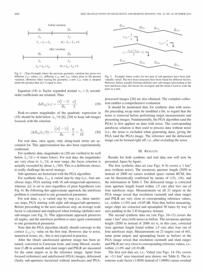
Fig. 4. (Top) Example where the previous geometry variation has given twodifferent L13 values, i.e., differing L12 and L23 values prior to the presentvariation. (Bottom) After varying the geometry, a new L13 value is adoptedunder the premise that ΔL is equal to zero.

Equation (18) is Taylor expanded around xs = 0; second-order coefficients are retained. Thus

ΔRsq(xs) =(s2f − 1)

Rb· x

2s

2. (19)

Peak-to-center magnitudes of the quadratic expression in(19) should be held below λc/16 [6], [20] to keep sub-imagesfocused, with the criterion

|ΔRsq(ls/2)| =

∣∣∣(s2f − 1)∣∣∣

Rb· l

2s

8<

λc

16. (20)

For real data, once again, only along-track terms are ac-counted for. This approximation has also been experimentallyconfirmed.

For synthetic data, magnitudes in (20) are verified to be wellbelow λc/16 (∼6 times lower). For real data, the magnitudesare very close to λc/16; at near range, the focus criterion isactually exceeded by about λc/300. This is a deliberate choice,to really challenge the novel strategy.

Sub-apertures are factorized with the FGA algorithm.For synthetic data, L13 is varied step by step (i.e., four aut-

ofocus steps, FGA starting with 16 sub-images/sub-apertures),whereas ΔL is set to zero regardless of prior hypotheses (seeFig. 4). By following this approximate approach, the autofocusproblem is constrained to one geometrical parameter.

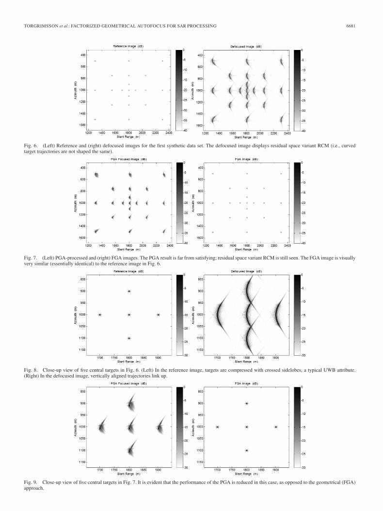
For real data, sf is varied step by step (i.e., three autofo-cus steps, FGA starting with eight sub-images/sub-apertures).Before proceeding to the next autofocus step, an average scalefactor is calculated and employed when forming (definite) newsub-images (see Fig. 5). This approximate approach preservesall angles, and the autofocus problem is once again constrainedto one geometrical parameter.

Note that the FGA algorithm ideally should converge to thecorrect L13/sf value on the first step. However, due to noise,numerical issues, etc., this is not expected in practice.

After the (final) autofocused aperture image has been at-tained, converted to Cartesian form, and ramp filtered, resolu-tion (3 dB in azimuth and slant range) and PSLR are measuredfor the same targets as in the reference image. Apart fromfocused (reference) and autofocused (FGA) images, defocused(faulty sub-apertures factorized without autofocus) and PGA-

Fig. 5. Example where scales for two pair of sub-apertures have been indi-vidually varied. The best focus measures have been found for different factors.However, before actually forming (definite) new sub-images (proceeding to thenext autofocus step), the factors are averaged, and the mean is used to scale thepairs as a unit.

processed images [20] are also obtained. The complete collec-tion enables a comprehensive evaluation.

It should be mentioned that, for synthetic data with noise,the preceding recap must be modified a bit, to regard that thenoise is removed before performing target measurements andpresenting images. Fundamentally, the FGA algorithm (and thePGA) is first applied on data with noise. The correspondingautofocus solution is then used to process data without noise(i.e., the noise is excluded when generating data), giving theFGA (and the PGA) image. The reference and the defocusedimage can be formed right off, i.e., after excluding the noise.

III. RESULTS

Results for both synthetic and real data sets will now bepresented, figure by figure.

The first synthetic data set (see Figs. 6–9) covers a 1 km2

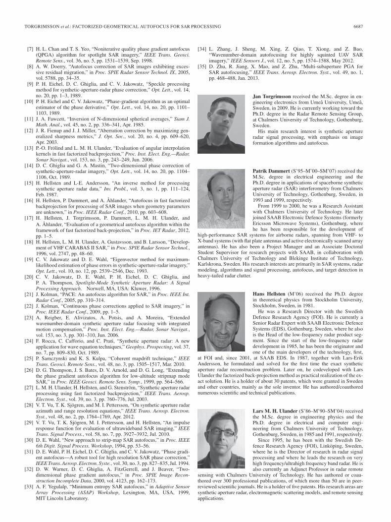
area (without noise). The erroneous aperture length (2050 minstead of 2000 m) causes residual space variant RCM; thiscan be theoretically confirmed by means of (15), (16), andthe information in Table I. The defocused image is corrected(true aperture length found within ±5 cm) after two out offour autofocus steps. Measurements on all 21 targets in theFGA image reveal that resolution (azimuth and slant range)and PSLR are very close to corresponding reference values,i.e., within ±1.0% and ±0.05 dB. Note that, before measuring,target chips are extracted and upsampled 50 times by way ofzero padding in the 2-D frequency domain.

The second synthetic data set (see Figs. 10–13) covers thesame 1 km2 area (with noise) as before. The erroneous aperturelength (2050 m instead of 2000 m) is, in this case, corrected(true aperture length found within ±5 cm) after four out offour autofocus steps. Measurements on 21 targets (out of 441,same point targets and upsampling factor as before) in theFGA image reveal that resolution (azimuth and slant range)and PSLR are very close to corresponding reference values, i.e.,within ±1.0% and ±0.10 dB.

The first real data set, i.e., Vidsel (see Figs. 14–18), coversan ∼3.5 km2 area (maximal area shown; see Table I). The er-roneous scale factor (1.0050 instead of 1.0000) causes residual


Fig. 6. (Left) Reference and (right) defocused images for the first synthetic data set. The defocused image displays residual space variant RCM (i.e., curvedtarget trajectories are not shaped the same).

Fig. 7. (Left) PGA-processed and (right) FGA images. The PGA result is far from satisfying; residual space variant RCM is still seen. The FGA image is visuallyvery similar (essentially identical) to the reference image in Fig. 6.

Fig. 8. Close-up view of five central targets in Fig. 6. (Left) In the reference image, targets are compressed with crossed sidelobes, a typical UWB attribute.(Right) In the defocused image, vertically aligned trajectories link up.

Fig. 9. Close-up view of five central targets in Fig. 7. It is evident that the performance of the PGA is reduced in this case, as opposed to the geometrical (FGA)approach.


Fig. 10. (Left) Reference and (right) defocused images for the second synthetic data set. The reference image has an ordered structure (targets placed 50 mapart), whereas the defocused image is very chaotic as trajectories interfere.

Fig. 11. (Left) PGA-processed and (right) FGA images. The PGA result is once again far from satisfying. The FGA image is visually very similar (essentiallyidentical) to the reference image in Fig. 10.

Fig. 12. Close-up view of nine central targets in Fig. 10. (Left) In the reference image, targets are compressed with crossed sidelobes, a typical UWB attribute.(Right) In the defocused image, vertically aligned trajectories overlap.

Fig. 13. Close-up view of nine central targets in Fig. 11. It is once again evident that the performance of the PGA is reduced, as opposed to the geometrical(FGA) approach.


Fig. 14. (Left) Reference and (right) defocused images for the first real data set (CARABAS II—Vidsel). The defocused image displays residual space invariantRCM.

Fig. 15. (Left) PGA-processed and (right) FGA images. The PGA result is not satisfying; residual space invariant RCM is still seen. The FGA image is visuallyvery similar to the reference image in Fig. 14.

Fig. 16. Close-up view of Fig. 14. The SNR degradation in the defocused image is obvious; the residual RCM is very observable as well.

Fig. 17. Close-up view of Fig. 15. The FGA result is promising; the PGA result, on the other hand, is not acceptable.


Fig. 18. (Left, top to bottom) Image chips for the trihedral; 3-dB areas are marked red. (Right, top to bottom) Three-dimensional mesh plots. Note in particularthat the mainlobe in the PGA image is blurred, with a weak (below the 3-dB level) RCM trace, i.e., although the PGA refines the defocused result, the compressionis incomplete.


Fig. 19. (Left) Reference and (right) defocused images for the second real data set (CARABAS II—Linköping). The defocused image displays residual spacevariant RCM.

Fig. 20. (Left) PGA-processed and (right) FGA images. The PGA result is not satisfying; residual space variant RCM is still seen. The FGA image is visuallyvery similar to the reference image in Fig. 19.

Fig. 21. Close-up view of Fig. 19. The SNR degradation in the defocused image is obvious; the residual RCM is very observable as well.

Fig. 22. Close-up view of Fig. 20. The FGA result is promising; the PGA result, on the other hand, is not acceptable.


space invariant RCM; this can also be theoretically confirmedby means of (15) and the information in Table I. As targetsare confined to a small area, i.e., substantially smaller than3.5 km2, space variant effects according to the criterion in(16) are not seen. The scale factor is estimated to ∼1.0049after one autofocus step; remaining steps do not correct thescale additionally. Measurements (after upsampling 25 times)on two pointlike targets (including the trihedral reflector) inthe FGA image reveal that mainlobes have been broadenedby ∼2% in azimuth (3.36–3.44 m for the reflector) and ∼1%in slant range (2.38–2.40 m for the reflector). A PSLR lossof approximately 0.2 dB (6.8–6.6 dB for the reflector) is alsoobserved. Despite the minor degradation (measured), the FGAimage is very similar to the reference image. Even when thetrihedral is shown alone (see Fig. 18), in form of image cutsand 3-D plots, it is hard to discern a difference.

The second real data set, i.e., Linköping (see Figs. 19–22),covers an ∼4.5 km2 area (maximal area shown; see Table I).The erroneous scale factor (1.0050 instead of 1.0000) causesresidual space variant RCM; this can also be theoreticallyconfirmed by means of (15), (16), and the information inTable I. The scale factor is estimated to ∼1.0050 after threeautofocus steps. Measurements (after upsampling 25 times) ontwo pointlike targets [located ∼1.5 km apart in slant range,satisfying the criterion in (16)] in the FGA image reveal thatthe resolution is preserved (no mainlobe broadening). A PSLRloss of approximately 0.2 dB is observed for the far rangetarget.

PGA-processed images [20] (for both synthetic and real datasets) are not pleasing; this is visually evident; hence, resolutionand PSLR have not been measured.

IV. DISCUSSION

A. Results and FGA

Results for synthetic and real data sets have now been pre-sented (see Figs. 6–22). It is obvious that focused (reference)and autofocused (FGA) images are very similar. Target mea-surements also confirm that the FGA algorithm can compensatefor residual space variant RCM. A visual inspection verifies thatthe PGA cannot. This is no surprise since the PGA is a stand-alone technique (i.e., a separate stage after SAR processing)neglecting the geometrical aspect. By adding an additionalautofocus stage or stages within the processing chain [8], [34],[35], it is possible to mitigate residual space invariant RCM.The hybrid approach takes the geometry into consideration, butnot completely. The FGA algorithm, on the other hand, is notintegrated separately. In fact, as soon as the strategy is activated,it is the processing chain, offering a complete geometricalsolution (in this paper though, the problems are confined to onegeometrical quantity for simplicity).

Apart from the FGA algorithm (and the early formulation[16]) and the 1-D technique described in [2], back-projectionadapted autofocus has been disregarded. This paper, however,promotes the advantages, and although the problems dealt withare constrained, the capacity of the novel strategy is demon-strated, encouraging future work.

B. Future Work

At the moment, the run time is the main obstacle. The ex-haustive search routine must be replaced by a faster alternative,as it makes the FGA algorithm too slow to be of practical use forreal-time applications. Gradient-descent-based schemes shouldbe surveyed prior to performing a full trial (i.e., correcting sixparameters).

The object function is also an important subject. Althoughintensity correlation has worked well thus far, there are numer-ous other functions to consider, e.g., contrast [21], [22], squaredintensity [12], entropy [33], etc. [note that these functions areapplied on the sum in (12) and not on the addends].

V. CONCLUSION

We have described and analyzed a new geometrical autofo-cus approach for SAR. The strategy, termed the FGA algorithm,is an FFBP realization with a number of adjustable geometryparameters for each factorization step. By altering the aperturetrack in the time domain, it is possible to correct an inaccurategeometry (potentially introduced due to relaxed requirementson the IMU/GPS and/or a jammed/shadowed GPS). This indi-cates that the FGA algorithm has the capacity to compensatefor residual space variant RCM.

The performance of the algorithm is demonstrated for ge-ometrically constrained autofocus problems, embracing bothsynthetic and real (CARABAS II) data sets. Resolution (3 dBin azimuth and slant range) and PSLR measurements on targets(point targets for synthetic data and pointlike targets for realdata) in FGA and reference images give similar results within afew percent and tenths of a decibel. The advantage of a geomet-rical autofocus approach is clarified further when comparingFGA and PGA-processed images [20].

ACKNOWLEDGMENT

The authors would like to thank Dr. A. Åhlander, J. Lindgren(SAAB Electronic Defence Systems), and Dr. L. Eriksson(Chalmers University of Technology) for their valuable inputs.The authors would also like to thank the anonymous reviewersfor their comments, helping to improve this paper.

REFERENCES

[1] L.-E. Andersson, “On the determination of a function from sphericalaverages,” Siam J. Math. Anal., vol. 19, no. 1, pp. 214–232, Jan. 1988.

[2] J. N. Ash, “An autofocus method for backprojection imagery in syntheticaperture radar,” IEEE Geosci. Remote Sens. Lett., vol. 9, no. 1, pp. 104–108, Jan. 2012.

[3] C. Cafforio, C. Prati, and F. Rocca, “SAR data focusing using seismicmigration techniques,” IEEE Trans. Aerosp. Electron. Syst., vol. 27, no. 2,pp. 194–207, Mar. 1991.

[4] H. Cantalloube and P. Dubois-Fernandez, “Airborne X-band SAR imagingwith 10 cm resolution: Technical challenge and preliminary results,” Proc.Inst. Elect. Eng.—Radar, Sonar Navigat., vol. 153, no. 2, pp. 163–176,Apr. 2006.

[5] H. M. J. Cantalloube and C. E. Nahum, “Multiscale local map-drift-drivenmultilateration SAR autofocus using fast polar format image synthesis,”IEEE Trans. Geosci. Remote Sens., vol. 49, no. 10, pp. 3730–3736,Oct. 2011.

[6] W. G. Carrara, R. S. Goodman, and R. M. Majewski, Spotlight SyntheticAperture Radar: Signal Processing Algorithms. Norwood, MA, USA:Artech House, 1995.


[7] H. L. Chan and T. S. Yeo, “Noniterative quality phase gradient autofocus(QPGA) algorithm for spotlight SAR imagery,” IEEE Trans. Geosci.Remote Sens., vol. 36, no. 5, pp. 1531–1539, Sep. 1998.

[8] A. W. Doerry, “Autofocus correction of SAR images exhibiting exces-sive residual migration,” in Proc. SPIE Radar Sensor Technol. IX, 2005,vol. 5788, pp. 34–35.

[9] P. H. Eichel, D. C. Ghiglia, and C. V. Jakowatz, “Speckle processingmethod for synthetic-aperture-radar phase correction,” Opt. Lett., vol. 14,no. 20, pp. 1–3, 1989.

[10] P. H. Eichel and C. V. Jakowatz, “Phase-gradient algorithm as an optimalestimator of the phase derivative,” Opt. Lett., vol. 14, no. 20, pp. 1101–1103, 1989.

[11] J. A. Fawcett, “Inversion of N-dimensional spherical averages,” Siam J.Math. Anal., vol. 45, no. 2, pp. 336–341, Apr. 1985.

[12] J. R. Fienup and J. J. Miller, “Aberration correction by maximizing gen-eralized sharpness metrics,” J. Opt. Soc., vol. 20, no. 4, pp. 609–620,Apr. 2003.

[13] P.-O. Frölind and L. M. H. Ulander, “Evaluation of angular interpolationkernels in fast factorized backprojection,” Proc. Inst. Elect. Eng.—Radar,Sonar Navigat., vol. 153, no. 3, pp. 243–249, Jun. 2006.

[14] D. C. Ghiglia and G. A. Mastin, “Two-dimensional phase correction ofsynthetic-aperture-radar imagery,” Opt. Lett., vol. 14, no. 20, pp. 1104–1106, Oct. 1989.

[15] H. Hellsten and L-E. Andersson, “An inverse method for processingsynthetic aperture radar data,” Inv. Probl., vol. 3, no. 1, pp. 111–124,Feb. 1987.

[16] H. Hellsten, P. Dammert, and A. Åhlander, “Autofocus in fast factorizedbackprojection for processing of SAR images when geometry parametersare unknown,” in Proc. IEEE Radar Conf., 2010, pp. 603–608.

[17] H. Hellsten, J. Torgrimsson, P. Dammert, L. M. H. Ulander, andA. Åhlander, “Evaluation of a geometrical autofocus algorithm within theframework of fast factorized back-projection,” in Proc. IET Radar, 2012,pp. 1–5.

[18] H. Hellsten, L. M. H. Ulander, A. Gustavsson, and B. Larsson, “Develop-ment of VHF CARABAS II SAR,” in Proc. SPIE Radar Sensor Technol.,1996, vol. 2747, pp. 48–60.

[19] C. V. Jakowatz and D. E. Wahl, “Eigenvector method for maximum-likelihood estimation of phase errors in synthetic-aperture-radar imagery,”Opt. Lett., vol. 10, no. 12, pp. 2539–2546, Dec. 1993.

[20] C. V. Jakowatz, D. E. Wahl, P. H. Eichel, D. C. Ghiglia, andP. A. Thompson, Spotlight-Mode Synthetic Aperture Radar: A SignalProcessing Approach. Norwell, MA, USA: Kluwer, 1996.

[21] J. Kolman, “PACE: An autofocus algorithm for SAR,” in Proc. IEEE Int.Radar Conf., 2005, pp. 310–314.

[22] J. Kolman, “Continuous phase corrections applied to SAR imagery,” inProc. IEEE Radar Conf., 2009, pp. 1–5.

[23] A. Reigber, E. Alivizatos, A. Potsis, and A. Moreira, “Extendedwavenumber-domain synthetic aperture radar focusing with integratedmotion compensation,” Proc. Inst. Elect. Eng.—Radar, Sonar Navigat.,vol. 153, no. 3, pp. 301–310, Jun. 2006.

[24] F. Rocca, C. Cafforio, and C. Prati, “Synthetic aperture radar: A newapplication for wave equation techniques,” Geophys. Prospecting, vol. 37,no. 7, pp. 809–830, Oct. 1989.

[25] P. Samczynski and K. S. Kulpa, “Coherent mapdrift technique,” IEEETrans. Geosci. Remote Sens., vol. 48, no. 3, pp. 1505–1517, Mar. 2010.

[26] D. G. Thompson, J. S. Bates, D. V. Arnold, and D. G. Long, “Extendingthe phase gradient autofocus algorithm for low-altitude stripmap modeSAR,” in Proc. IEEE Geosci. Remote Sens. Symp., 1999, pp. 564–566.

[27] L. M. H. Ulander, H. Hellsten, and G. Stenström, “Synthetic aperture radarprocessing using fast factorized backprojection,” IEEE Trans. Aerosp.Electron. Syst., vol. 39, no. 3, pp. 760–776, Jul. 2003.

[28] V. T. Vu, T. K. Sjögren, and M. I. Pettersson, “On synthetic aperture radarazimuth and range resolution equations,” IEEE Trans. Aerosp. Electron.Syst., vol. 48, no. 2, pp. 1764–1769, Apr. 2012.

[29] V. T. Vu, T. K. Sjögren, M. I. Pettersson, and H. Hellsten, “An impulseresponse function for evaluation of ultrawideband SAR imaging,” IEEETrans. Signal Process., vol. 58, no. 7, pp. 3927–3932, Jul. 2010.

[30] D. E. Wahl, “New approach to strip-map SAR autofocus,” in Proc. IEEE6th Digit. Signal Process. Workshop, 1994, pp. 53–56.

[31] D. E. Wahl, P. H. Eichel, D. C. Ghiglia, and C. V. Jakowatz, “Phase gradi-ent autofocus—A robust tool for high resolution SAR phase correction,”IEEE Trans. Aerosp. Electron. Syste., vol. 30, no. 3, pp. 827–835, Jul. 1994.

[32] D. W. Warner, D. C. Ghiglia, A. FitzGerrell, and J. Beaver, “Two-dimensional phase gradient autofocus,” in Proc. SPIE Image Recon-struction Incomplete Data, 2000, vol. 4123, pp. 162–173.

[33] A. F. Yegulalp, “Minimum entropy SAR autofocus,” in Adaptive SensorArray Processing (ASAP) Workshop, Lexington, MA, USA, 1999,MIT Lincoln Laboratory.

[34] L. Zhang, J. Sheng, M. Xing, Z. Qiao, T. Xiong, and Z. Bao,“Wavenumber-domain autofocusing for highly squinted UAV SARimagery,” IEEE Sensors J., vol. 12, no. 5, pp. 1574–1588, May 2012.

[35] D. Zhu, R. Jiang, X. Mao, and Z. Zhu, “Multi-subaperture PGA forSAR autofocusing,” IEEE Trans. Aerosp. Electron. Syst., vol. 49, no. 1,pp. 468–488, Jan. 2013.

Jan Torgrimsson received the M.Sc. degree in en-gineering electronics from Umeå University, Umeå,Sweden, in 2009. He is currently working toward thePh.D. degree in the Radar Remote Sensing Group,at Chalmers University of Technology, Gothenburg,Sweden.

His main research interest is synthetic apertureradar signal processing, with emphasis on imageformation algorithms and autofocus.

Patrik Dammert (S’95–M’00–SM’07) received theM.Sc. degree in electrical engineering and thePh.D. degree in applications of spaceborne syntheticaperture radar (SAR) interferometry from ChalmersUniversity of Technology, Gothenburg, Sweden, in1993 and 1999, respectively.

From 1999 to 2000, he was a Research Assistantwith Chalmers University of Technology. He laterjoined SAAB Electronic Defence Systems (formerlyEricsson Microwave Systems), Gothenburg, wherehe has been responsible for the development of

high-performance SAR systems for airborne radars, spanning from VHF- toX-band systems (with flat plate antennas and active electronically scanned arrayantennas). He has also been a Project Manager and an Associate DoctoralStudent Supervisor for research projects with SAAB, in collaboration withChalmers University of Technology and Blekinge Institute of Technology,Karlskrona, Sweden. His research interests are primarily in SAR systems, radarmodeling, algorithms and signal processing, autofocus, and target detection inheavy-tailed radar clutter.

Hans Hellsten (M’06) received the Ph.D. degreein theoretical physics from Stockholm University,Stockholm, Sweden, in 1981.

He was a Research Director with the SwedishDefence Research Agency (FOI). He is currently aSenior Radar Expert with SAAB Electronic DefenceSystems (EDS), Gothenburg, Sweden, where he alsois the Head of the low-frequency radar product seg-ment. Since the start of the low-frequency radardevelopment in 1985, he has been the originator andone of the main developers of the technology, first,

at FOI and, since 2001, at SAAB EDS. In 1987, together with Lars-ErikAndersson, he formulated and solved for the first time the exact syntheticaperture radar reconstruction problem. Later on, he codeveloped with LarsUlander the factorized back-projection method as practical realization of the ex-act solution. He is a holder of about 30 patents, which were granted in Swedenand other countries, mainly as the sole inventor. He has authored/coauthorednumerous scientific and technical publications.

Lars M. H. Ulander (S’86–M’90–SM’04) receivedthe M.Sc. degree in engineering physics and thePh.D. degree in electrical and computer engi-neering from Chalmers University of Technology,Gothenburg, Sweden, in 1985 and 1991, respectively.

Since 1995, he has been with the Swedish De-fence Research Agency (FOI), Linköping, Sweden,where he is the Director of research in radar signalprocessing and where he leads the research on veryhigh frequency/ultrahigh frequency band radar. He isalso currently an Adjunct Professor in radar remote

sensing with Chalmers University of Technology. He has authored or coau-thored over 300 professional publications, of which more than 50 are in peer-reviewed scientific journals. He is a holder of five patents. His research areas aresynthetic aperture radar, electromagnetic scattering models, and remote sensingapplications.

factorized geometrical autofocus for synthetic aperture...

Documents