1

Author version: Clim. Dyn., vol.37; 2011; 493-507

Factors controlling January-April rainfall over southern India and Sri Lanka

J. Vialard1 2, P. Terray1, J-P. Duvel3, R.S. Nanjundiah4, S.S.C. Shenoi5, D. Shankar2

1. Laboratoire d'Océanographie Expérimentation et Approches Numériques, CNRS, UPMC, IRD, Paris, France

2. National Institute of Oceanography, Goa, India

3. Laboratoire de Météorologie Dynamique, CNRS, Paris, France.

4. Center of Atmospheric and Oceanic Sciences, IISc, Bangalore, India

5. Indian National Centre for Ocean Information Services, Hyderabad, India

Submitted to Climate Dynamics: 17 August 2011 Corresponding author address: Dr. Jérôme Vialard, LOCEAN – Case 100 Université Pierre et Marie Curie 75232 Paris Cedex 05 - Fance E-mail: jv@locean-ipsl.upmc.fr

Abstract

Most of the annual rainfall over India occurs during the Southwest (June-September) and Northeast (October-December) monsoon periods. In March 2008, however, Southern peninsular India and Sri Lanka received the largest rainfall anomaly on record since 1979, with amplitude comparable to summer-monsoon interannual anomalies. This anomalous rainfall appeared to be modulated at intraseasonal timescale by the Madden Julian Oscillation, and was synchronous with a decaying La Niña event in the Pacific Ocean. Was this a coincidence or indicative of a teleconnection pattern? In this paper, we explore factors controlling rainfall over southern India and Sri Lanka between January and April, i.e., outside of the southwest and northeast monsoons. This period accounts for 20% of annual precipitation over Sri Lanka and 10 % over the southern Indian states of Kerala and Tamil Nadu. Interannual variability is strong (about 40% of the January-April climatology). Intraseasonal rainfall anomalies over southern India and Sri Lanka are significantly associated with equatorial eastward propagation, characteristic of the Madden Julian oscillation. At the interannual timescale, we find a clear connection with El Niño-Southern Oscillation (ENSO); with El Niños being associated with decreased rainfall (correlation of -0.46 significant at the 98% level). There is also a significant link with local SST anomalies over the Indian Ocean, and in particular with the inter-hemispheric sea surface temperature (SST) gradient over the Indian Ocean (with colder SST south of the equator being conducive to more rainfall, correlation of 0.55 significant at the 99% level). La Niñas / cold SSTs south of the equator tend to have a larger impact than El Niños. We discuss two possible mechanisms that could explain these statistical relationships: 1) subsidence over southern India remotely forced by Pacific SST anomalies; 2) impact of ENSO-forced regional Indian Ocean SST anomalies on convection. However, the length of the observational record does not allow distinguishing between these two mechanisms in a statistically significant manner.

2

1. Introduction

About 90% of the annual rainfall over India falls during the southwest (June to September) and

northeast (October to December) monsoons. These two monsoons have a great influence over the

livelihoods of over one billion people living in India and Sri Lanka. There is, for example, a clear

link between the monsoon rainfall and rice production in India (see, e.g. Webster et al., 1998 for a

description of the socio-economic impacts of the monsoon over India). This has prompted numerous

studies on factors controlling the variations of the southwest monsoon at both interannual and

intraseasonal timescales.

The seminal work of Sir Gilbert Walker (e.g. Walker and Bliss, 1932) both pointed out the link

between the Indian monsoon and sea level pressure at Darwin, Australia, and led to the discovery of

what would be later known as El Niño / Southern Oscillation (ENSO). Many studies then illustrated

the links between ENSO and the southwest monsoon, suggesting that anomalously warm

temperatures in the central Pacific during El Niño induce anomalous subsidence further west, over

India, which tend to diminish convection and rainfall (Shukla and Paolino 1983; Rasmusson and

Carpenter 1983; Ropelewski and Halpert 1987, 1989, Nageswara Rao 1999). This relation between

ENSO and the southwest monsoon however appears to have weakened during recent decades (e.g.

Krishna Kumar et al. 1999). There is also an influence of ENSO on the northeast monsoon

(Ropelewski and Halpert 1987, 1989, Nageswara Rao 1999, Kripalani and Pankaj Kumar 2004,

Pankaj Kumar et al. 2007, Revadekar and Kulkarni 2008), with an El Niño being associated with

increased northeast monsoon rainfall over southern India and Sri Lanka between October and

December. This relation seems to have strengthened during the last decades, unlike the ENSO-

southwest monsoon teleconnection (Zubair and Ropelewski 2006, Pankaj Kumar et al. 2007), and is

generally attributed to ENSO-induced changes in the Walker circulation.

In addition to atmospheric teleconnections associated with changes in the Walker circulation,

there is also the possibility that local SST changes in the Indian Ocean could affect the monsoon.

There is clear SST interannual variability in the Indian Ocean. One part is associated with a warming

of the Indian Ocean during El Niños (cooling during La Niñas), remotely forced by increased

subsidence (ascendance) over the Indian Ocean (Klein et al. 1999; Lau and Nath 2000). Another part

is associated with an intrinsic mode of variability of the Indian Ocean. As ENSO in the Pacific, the

“Indian Ocean dipole” (IOD; e.g. Saji et al. 1999; Webster et al. 1999; Murtugudde et al. 2000)

develops as the result of an ocean-atmosphere coupled instability, and leads to an east-west dipole in

SST and associated zonal wind anomaly. While there is a tendency of the IOD to occur

3

simultaneously with El Niño, this ENSO influence is not a one-to-one relationship (e.g. Yamagata et

al. 2004).

Several studies have shown clear links between Indian Ocean SST anomalies (either intrinsic

or linked to ENSO) and the Indian monsoons (see Schott et al. 2009 for a review). The maximum

IOD SST perturbations occur during the northeast Monsoon. Zubair et al. (2003) investigated their

link and suggested a role of Indian Ocean SSTs in modulating the northeast monsoon. SST

anomalies that develop in the southwestern tropical Indian Ocean and in the Somalia upwelling

during the course of an IOD or after an ENSO event impact rainfall over the Western Ghats of India

during the following southwest monsoon (Izumo et al 2008; Vecchi and Harrison 2004). Annamalai

et al. (2005) showed that Indian Ocean Sea Surface Temperature Anomalies (SSTAs) affect the

atmospheric integrated moisture and can induce an advance or delay in the onset of the southwest

monsoon. Finally, recent studies illustrate how both ocean dynamical processes (Du et al., 2009) and

wind-evaporation-SST feedback (Wu et al. 2008, Kawamura et al. 2001) tend to induce an

asymmetric SST response to ENSO, with warm SSTAs south of the equator during spring, which

migrate to the northern Indian Ocean in summer. These SSTAs are associated with an asymmetric

atmospheric response in spring, with reduced precipitation over the Arabian Sea, Bay of Bengal and

South China Sea (Xie et al. 2009, Wu et al. 2008).

In addition to interannual anomalies, the other clear signals in monsoon rainfall are

intraseasonal variations, with “active” and “break” spells of the Indian monsoon. During summer, in

addition to synoptic variability, there is indeed a clear modulation of the monsoon at two preferential

timescales around 10-20 and 30-60 days (e.g Goswami 2005; Waliser 2006). The 30-60 day

modulation of monsoon rainfall is associated with a clear northward propagation of convective

anomalies over India and the Bay of Bengal. The main mode of atmospheric intraseasonal variability

is the Madden-Julian oscillation (hereafter MJO, see e.g. Zhang, 2005 for a review), which is rather

associated with eastward propagation of convective anomalies along the convergence zone. Active

and break cycles of the monsoon tend to be associated with the MJO over the Indian Ocean, although

this relation is not systematic (see, e.g., Goswami 2005 for a discussion). MJO composites indeed

show northward propagation of convective perturbations over India during summer (e.g. Wheeler

and Hendon, 2004), characteristic of the monsoon active and break phases.

There have thus been numerous studies of the factors controlling interannual and intraseasonal

variability of the northeast and southwest monsoon. In contrast, there are almost no studies of the

factors controlling the rain over Southern India and Sri Lanka outside of the two monsoons season

(roughly between January and May). Most of the studies investigating the impacts of the ENSO

4

cycle on rainfall over Asia and the Western Pacific during spring have focused on the Indonesian and

east Asian monsoon, where signals are strongest (see, e.g., Wang et al. 2000), but not on India. The

recent studies of Wu et al. (2008) and Xie et al. (2009) focus on large-scale rainfall patterns over the

Indian Ocean during spring, but do not study specifically rainfall anomalies over southern India and

Sri Lanka. Although the total rainfall during this period is rather low (around 10 cm over southern

India and 30 cm over Sri Lanka), it accounts for 20% of annual precipitation over Sri Lanka and 10

% over the southern Indian states of Kerala and Tamil Nadu (see Fig. 1a, b). Interannual variability

is strong (about 40% of the mean, Fig. 1c). This can easily be understood since the southern tip of

India and Sri Lanka lies at the fringe of the Inter-Tropical Convergence Zone (ITCZ) at that time:

small latitudinal shifts of the ITCZ can thus result in rather large precipitation anomalies in this

region during spring. Another motivation is given by a recent event. In March 2008, there was a

strong rainfall anomaly over most of peninsular India, south of 20°N (Fig. 2a). This was the largest

anomaly over southern India and Sri Lanka (hereafter SISL) since 1979, even when monsoon month

anomalies are included. There was also a clear rainfall anomaly in April 2008, although mostly over

the Bay of Bengal, and there was a decaying La Niña in the Pacific Ocean and cold SST anomalies

in the southern Indian Ocean (see Fig. 2b, c). Are those two large anomalous rain-events in March

and April 2008 connected with the decaying La Niña in the Pacific Ocean and/or local SSTAs in the

Indian Ocean? In this paper, we will investigate the factors controlling rainfall over SISL during

January-April.

The paper is constructed as follows. Section 2 presents the data and methods used in this paper.

In section 3, we present the case of the March 2008 rainfall anomaly as an example. We show that

the March 2008 rainfall anomalies over India were synchronous with a La Niña in the Pacific Ocean

and a cold south Indian Ocean. Rainfall anomalies over SISL also appeared to be modulated by the

MJO at the intraseasonal timescale. In section 4, we explore teleconnections associated with winter

and spring rainfall over south peninsular India. We show that it is modulated by the MJO at

intraseasonal timescale, and significantly correlated with ENSO at the interannual timescale. We also

explore links between January-April SISL rainfall and SST anomalies in the Indian Ocean and find a

significant connection with the interhemispheric SST gradient. A summary and discussion of these

results are provided in section 5, which includes hypotheses of mechanisms and links of our results

with other recent studies.

5

2. Data and methods

a. Data

The rainfall dataset we use is the Global Precipitation Climatology Project (GPCP; Huffman et

al 1997). In most of the paper, we use the pentad data, available on a 2.5° grid since January 1979.

However, we use the daily data on a 1° grid (Huffman et al. 2001) to illustrate the March 2008

anomalous rain event. We use pentad data rather than monthly data since, as we will show later, the

rainfall over India is modulated at intraseasonal timescale by the MJO. Using 5-day data allows

filtering out the MJO signal by applying a 90-day low-pass filter (see section 2.b), hence avoiding

the strong aliasing on monthly data, and resulting in a better isolation of ENSO teleconnections. We

will also use the high-resolution gridded daily precipitation dataset produced by the India

Meteorological Department (Rajeevan et al., 2006). This is probably the best available rainfall

dataset for India. Hence, we repeated some of the diagnostics made with GPCP data with the IMD

data, to check that the ENSO-rainfall teleconnection is robust when considering only southern India

and the late winter and early spring season.

We use the monthly gridded SST product from Reynolds et al. (2002). This product is

available on a 1° regular grid from November 1981 to present. We use velocity potential at sigma

level (sigma=0.22, i.e. very close to the 225 hPa level) from the NCEP-NCAR reanalysis (Kalnay et

al. 1996) as a proxy for the Walker circulation. This proxy has also been used in previous studies

(e.g. Krishna Kumar et al., 1999; Zubair and Ropelewski 2006). This data was downloaded from the

Climate Data Centre (CDC) website at http://www.cdc.noaa.gov/. We use monthly data from 1958 to

present at a resolution of 1.875°.

Scatterometer winds from Quickscat will be used to illustrate the wind climatology during

different seasons over the Indian Ocean. The wind product produced by CERSAT (IFREMER) is

available at http://www.ifremer.fr/cersat/en/index.htm

To study the influence of the MJO, we have used the index developed by Wheeler and Hendon

(2004). This index is available online at

http://www.bom.gov.au/bmrc/clfor/cfstaff/matw/maproom/RMM/

b. Methods

In this paper, we will mainly use linear-regression diagnostics to illustrate statistical relations

between existing climate indices and rainfall over south India. All the regression analyses in this

6

paper use standardized indices (i.e. of standard deviation equal to 1), in order to isolate the amplitude

of rainfall anomalies associated with, e.g., a “typical” amplitude El Niño event.

The regression analyses aiming at isolating the influence of El Niño use a rather classical

index: the December value of the average Nino3.4 region (120°W-170°W, 5°N-5°S) SST normalized

anomaly. The list of years obtained with this criterion is slightly different than, e.g., the list of ENSO

years as defined by the Climate Prediction Centre (CPC) (and available from

http://www.cpc.noaa.gov/products/analysis_monitoring/ensostuff/ensoyears.shtml ) but regressions

performed using both definitions look very similar. The other climate indices used in this paper will

be introduced in more detail later, but we will mention them quickly here. We use the same index as

Wu et al. (2008) to isolate the spring antisymmetric mode in rainfall (principal component of the first

EOF of average March-May precipitation over the Indian Ocean). We tested that this index is weakly

modified when applied over a different season (January-April instead of March-May) and different

period (1982-2008 in this study against 1979-2005 in Wu et al. 2008) and use the index derived over

March-May from 1982-2008 in this study. We use the difference of interannual anomalies of average

SST within (65°E-100°E, 10°N-20°N) and (75°E-105°E, 8°S-0°) to estimate the influence of

anomalies of the interhemispheric SST gradient (see later in the text for justification of the choice of

these regions). The southwestern Indian Ocean (hereafter SWIO, Annamalai et al. 2005) is an

important region for the Indian Ocean climate; for this region we use the same SST index as given in

Annamalai et al (2005) (SST anomalies averaged over 50-70°E, 17.5°S-7.5°S). Finally, we also use

the index of the “Subtropical Dipole mode” introduced by Behera and Yamagata (2001): SST

anomalies differences between the (90°E-100°E, 28°S-18°S) and (55°E-65°E, 37°S-27°S) regions.

All the analyses made in this paper are based on pentad data. A daily climatology is

constructed from the full record average of daiy-interpolated pentad data, with a 45-day boxcar filter

in order to remove aliasing from high frequencies. Interannual anomalies were first computed for

these pentad data by taking the difference between the raw data and this climatology. Time filtering

was then used to separate the intraseasonal (10-90 days) and seasonal (90 day+) components of these

interannual anomalies. We used several types of filters (simple filter based on a reverse Fourier

transform, digital filtering, Hanning filter) with a minor influence on our results. In the rest of the

paper, we use the simple Fourier filtering. We will refer the 90-day low-passed anomalies with

respect to the climatology as interannual anomalies. We define intraseasonal anomalies as the 10-90

day filtered anomalies with respect to the climatology. For all the significance computations, the

number of degrees of freedom has been taken as the number 90 days-samples for intraseasonally

filtered data, and number of years for interannual anomalies.

7

All the analyses have been made both on raw and detrended data, with very similar results.

Some studies have shown changes in teleconnections patterns (e.g. southwest monsoon and ENSO)

after the end of the seventies. All of the analyses in this paper are focusing on the recent period, and

are performed on the longest dataset available (1979-2007 or 1982-2007). We chose to exclude 2008

from these analyses, because of this very strong amplitude (see next section). Similar analyses up to

2009 included give similar results (with larger amplitude signals).

3. The case of March 2008

There was a clear rainfall anomaly over the central and eastern Indian Ocean in March and

April 2008 (Fig. 2a, b), with significant regions of monthly rainfall above 90 mm. While rainfall

anomalies were largely located over the ocean in April, there was a significant rainfall anomaly over

land (peninsular India and Sri Lanka) in March 2008. The largest rainfall anomalies over peninsular

India generally occur during the southwest monsoon. The March 2008 rainfall anomaly, however,

was the largest on record over that region (120 mm in one month) with values exceeding even those

of summer months (Fig. 3). Nevertheless, even though the March 2008 case is exceptional, there are

other occurrences of significant monthly rainfall anomalies during January-April (Fig. 3).

The Indo-Pacific climate in March 2008 was characterized by a decaying La Niña event. In March

2008, there were still significant cold anomalies near the dateline (up to -2°C anomaly, Fig. 2c).

There is thus a possibility that the March-April 2008 rainfall anomalies over India were in some

ways linked to this La Niña in the Pacific Ocean, and we’ll investigate this in the next section. But

local SST anomalies over the Indian Ocean could also play some role. The usual response to a La

Niña event at this time of the year is an overall cooling of the southern tropical Indian Ocean,

remotely forced by increased deep atmospheric convection over the Indian Ocean (Klein et al. 1999;

Lau and Nath 2000). In spring, this cooling is generally strongest south of the equator (Wu et al.

2008, Du et al. 2009, Xie et al. 2009). In March 2008, the Indian Ocean was indeed cooler over most

of the basin, with the clearest cooling between 20°S and the equator (Fig. 2c). A positive meridional

SST gradient can favour northward displacement of the ITCZ, both just before monsoon onset

(Annamalai et al. 2005) and during the monsoon (Shankar et al 2007). Figure 4a shows an estimate

of the climatological interhemispheric temperature gradient over the central and eastern Indian

Ocean. During normal years, the northern hemisphere becomes progressively warmer than the

southern hemisphere in March and rainfall starts (Fig. 4a) to increase over southern India. In 2008,

largely because of cold anomalies in the southern hemisphere, the February and March

8

climatological gradient had reversed. Warmer temperatures were found north of the equator, with an

inter-hemispheric gradient comparable to that of April during Normal years. This anomaly might

have contributed to favour an early northward displacement of the ITCZ in March 2008.

Figure 4b shows daily rainfall in late 2007 and early 2008 over the region outlined in figure 2a,

b. The rain event in March 2008 was a 20-25 days spell from the 5 March until the end of the month.

Figure 4b indicates that the rain event of March 2008 occurs during an active phase of the MJO over

the eastern Indian Ocean. Actually, figure 8 from Wheeler and Hendon (2004) suggests that the

averaged MJO perturbation in December-February span a large latitude range (about 15°S to 10°N),

and could have a signature over India The rain event of March 2008 occurred simultaneously with an

active phase of the MJO over the Indian Ocean. Actually, figure 8 from Wheeler and Hendon (2004)

suggests that the MJO in December-February spans a large latitude range (about 15°S to 10°N), and

could have a signature over India. We will investigate later if this can also be the case in March.

In the rest of the paper, we will investigate if the occurrence of a La Niña event and/or an

active phase of the MJO over the eastern Indian Ocean can give a large and positive rainfall anomaly

over southern India during the JFMA season.

4. Observed teleconnections associated with winter/spring rainfall over southern India and Sri Lanka

a. Rainfall patterns during January-April

Before proceeding to the discussion of the link between rainfall over south India and Sri Lanka

and El Niño during the dry season and the MJO, we will review briefly the structure of low-level

winds and rainfall at that time of the year. Figure 5 shows the surface wind and rainfall climatology.

During the southwest monsoon, the southwesterlies collect moisture over the southern Indian Ocean,

Arabian Sea and Bay of Bengal, with maximum precipitation downstream over the Western Ghats

and Myanmar region (Fig. 5a). The precipitation over southern India is thus largely the result of

moisture collected over the Arabian Sea by the monsoon low-level jet. During the northeast

monsoon, the winds have reversed and the precipitation over South India is mostly the result of

moisture collected over the Bay of Bengal by the easterlies. During January to March, the wind and

rain patterns do not change much (not shown). The wind becomes more southward as the ITCZ

moves southward under the effect of solar forcing. As a result, southern India receives much less

9

moisture and only the southern part of Sri Lanka experiences rainfall (Fig. 5c). The wind pattern

changes in April. With the strong and abrupt warming of the south-eastern Arabian Sea and southern

Bay of Bengal (not shown; Joseph, 1990; Vinayachandran and Shetye, 1991), the ITCZ moves north

of the equator in the central and eastern Indian Ocean, but the atmospheric circulation remains

anticyclonic over the Arabian Sea. As a result, surface winds become northwesterlies at the southern

tip of India and they bring moisture to these regions and significant rainfall start to occur there.

We have seen above that moisture sources and atmospheric circulation patterns appeared to be

quite different during January-March and April. To characterize the rainfall interannual patterns

during that period, we performed an EOF analysis of interannual GPCP rainfall anomalies separately

for months from December to May (Figure 6). The interannual variability during JFMA is strongest

south of the Bay of Bengal, but it extends over the SISL region. This impact is strongest during

January to March, but is also present in April.

The patterns of interannual variability are quite stable from January to April (their correlation

with the January-April average pattern are 0.96, 0.98, 0.93 and 0.67, respectively). On the other

hand, the patterns are markedly different for December and May (their correlation with the January-

April average pattern are 0.36 and -0.6, respectively). Because of the similarity of interannual

rainfall anomalies over the Northern Indian Ocean during the January to April months, we will

generally use the January-April average for our analyses in the rest of the paper.

b. MJO influence

We will first review the potential influence of the MJO on SISL precipitation. The March 2008

case suggests that rainfall tends to occur preferably during active phase of the MJO over the Indian

Ocean [i.e. the strong rainfall event over the SISL in March 2008 is related to a large-scale

convective intraseasonal event]. Similarly, figure 8 from Wheeler and Hendon (2004) shows that

active phase of the MJO is associated with low outgoing longwave radiation (i.e. more convection)

over southern India during December-February. Conversely, break phases of the MJO over the

Indian Ocean seem to be associated with less convection. Hence, we repeated the composite analysis

of Wheeler and Hendon (2004), but using GPCP pentad rainfall (rather than OLR) and focusing on

the January-March period.

Figure 7c shows that there is a statistically significant impact of the MJO on rainfall over

southern India with phase 3 (active convection over the Indian Ocean) associated with ~1.5 mm.day-

1 additional rainfall over south India while phases 6 and 7 (pause of convection over the Indian

Ocean) associated with small negative (~-.5 mm.day-1) rainfall anomalies. The composite map of

10

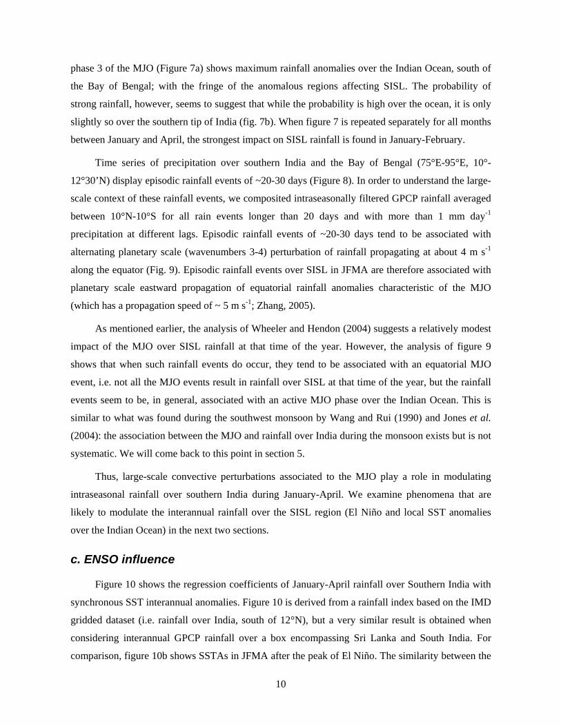
phase 3 of the MJO (Figure 7a) shows maximum rainfall anomalies over the Indian Ocean, south of

the Bay of Bengal; with the fringe of the anomalous regions affecting SISL. The probability of

strong rainfall, however, seems to suggest that while the probability is high over the ocean, it is only

slightly so over the southern tip of India (fig. 7b). When figure 7 is repeated separately for all months

between January and April, the strongest impact on SISL rainfall is found in January-February.

Time series of precipitation over southern India and the Bay of Bengal (75°E-95°E, 10°-

12°30’N) display episodic rainfall events of ~20-30 days (Figure 8). In order to understand the large-

scale context of these rainfall events, we composited intraseasonally filtered GPCP rainfall averaged

between 10°N-10°S for all rain events longer than 20 days and with more than 1 mm day-1

precipitation at different lags. Episodic rainfall events of ~20-30 days tend to be associated with

alternating planetary scale (wavenumbers 3-4) perturbation of rainfall propagating at about 4 m s-1

along the equator (Fig. 9). Episodic rainfall events over SISL in JFMA are therefore associated with

planetary scale eastward propagation of equatorial rainfall anomalies characteristic of the MJO

(which has a propagation speed of ~ 5 m s-1; Zhang, 2005).

As mentioned earlier, the analysis of Wheeler and Hendon (2004) suggests a relatively modest

impact of the MJO over SISL rainfall at that time of the year. However, the analysis of figure 9

shows that when such rainfall events do occur, they tend to be associated with an equatorial MJO

event, i.e. not all the MJO events result in rainfall over SISL at that time of the year, but the rainfall

events seem to be, in general, associated with an active MJO phase over the Indian Ocean. This is

similar to what was found during the southwest monsoon by Wang and Rui (1990) and Jones et al.

(2004): the association between the MJO and rainfall over India during the monsoon exists but is not

systematic. We will come back to this point in section 5.

Thus, large-scale convective perturbations associated to the MJO play a role in modulating

intraseasonal rainfall over southern India during January-April. We examine phenomena that are

likely to modulate the interannual rainfall over the SISL region (El Niño and local SST anomalies

over the Indian Ocean) in the next two sections.

c. ENSO influence

Figure 10 shows the regression coefficients of January-April rainfall over Southern India with

synchronous SST interannual anomalies. Figure 10 is derived from a rainfall index based on the IMD

gridded dataset (i.e. rainfall over India, south of 12°N), but a very similar result is obtained when

considering interannual GPCP rainfall over a box encompassing Sri Lanka and South India. For

comparison, figure 10b shows SSTAs in JFMA after the peak of El Niño. The similarity between the

11

ENSO pattern (Fig. 7b) and the teleconnection pattern of winter / spring SISL rainfall is striking.

Excess rainfall over southern India during this season is associated with a La Niña-like pattern in the

tropical Pacific and cold SST between the equator and 10°S in the Indian Ocean. There is also a very

clear and significant ENSO “horseshoe” pattern associated with rainfall over southern India in

JFMA.

It is interesting to note, however, that while the patterns are quite similar over the Pacific

Ocean, there are quite a few differences in patterns between figure 7a and 7b over the Indian Ocean.

This suggests that local SSTAs over the Indian Ocean might be important in triggering rainfall

anomalies over south India during JFMA. We will come back to this point in the section 4d.

Figure 11 shows the regression patterns of GPCP rainfall over the Indian Ocean for the

Niño3.4 SSTA in December (a good proxy for ENSO; we obtain similar pictures for other

commonly used ENSO indices). We show this regression for several seasons in order to compare the

signals in January-April with those already discussed for other seasons in previous studies.

Teleconnection patterns already discussed by other authors for both monsoons can be recognized. A

significant signal appears during the southwest monsoon over the Ghats as discussed by Vecchi and

Harrison (2004), with opposite phase on the year before and after the El Niño peak (Fig. 11a, d).

After the peak of El Niño, in agreement with the scenario proposed by (Izumo et al. 2008), the

rainfall anomaly is positive over the Ghats, as described in Vecchi and Harrison (2004). The opposite

phase observed the previous year is probably linked to the biennial nature of the interannual

variability over the Indian Ocean (Meehl et al., 2003). In October-November before its peak, El Niño

is associated with increased rainfall over SISL, as discussed in Ropelewski and Halpert (1987, 1989)

and Zubair and Ropelewski (2006).

But there is also a significant signal outside of the monsoon period. Figure 11c confirms that

an El Niño peak is followed by deficient rainfall (and La Niña with excess rainfall) over the southern

tip of India and Sri Lanka from January to April. Figure 12 shows the seasonal variations of the

regression coefficients of the average GPCP rainfall over SISL (72°E-82°30’E, 5°N-12°30’N) with

the December Niño3.4 normalized index. The strongest correlation with ENSO over that region is

during the northeast monsoon, in October-November, as reported in Ropelewski and Halpert (1987,

1989) and Zubair and Ropelewski (2006). Despite much weaker climatological rainfall in January-

February, the correlation found in this paper is almost as strong. The January-February typical

accumulated rainfall anomaly is 5.4 cm per anomalous standard deviation in Niño3.4 (Fig. 12a); for

an average rainfall of 12 cm (Fig 12b), i.e. almost 50% of the mean rainfall. Therefore, relative to the

12

mean rainfall, the influence of ENSO in this season is strong, with negative values. In absolute

terms, it is almost as strong as the signal in October-November.

Figure 13a shows a scatterplot between southern Indian monthly rainfall and Niño3.4 SSTA

interannual anomalies during January-April. This scatterplot reveals two interesting points. First

there is an asymmetry between the impact of El Niños and La Niñas. This is easily understandable.

The climatological rainfall at this season is quite low (about 30 cm in total from January to April)

and there’s thus a lower limit to the deficit rainfall anomalies associated with El Niños. On the other

hand, La Niñas can have a larger impact on excess rainfall. However, there is a larger spread in

rainfall anomalies for negative Nino3.4 SST anomalies, probably due to the high level of internal

variability inherent to rainfall dynamics. However, most of the significant (> 1 std) excess rainfall

anomalies are associated with cold Pacific SST anomalies while most of the deficit rainfall occurs

with warm Niño3.4. La Niña (El Niño) thus seems to be a necessary condition for increased

(reduced) rainfall over SISL in winter/spring, but not a sufficient one.

We summarize our main points in this section: 1) El Niños are associated with decreased

rainfall over India and Sri Lanka during JFMA; 2) La Niñas have the opposite effect, but with a

stronger amplitude. In the following section, we will test the potential influence of local SST

anomalies in the Indian Ocean on JFMA rainfall over the SISL region.

d. Indian Ocean SST influence

One must be careful and not attribute entirely the changes of rainfall over SISL to SST changes in

the tropical Pacific. Several modelling studies suggest that the SST changes associated with ENSO in

the tropical Indian Ocean (that are persistent until August the following year at least) can also have

an impact regionally (e.g. Watanabe and Jin 2003; Annamalai et al. 2005, Xie et al. 2009). La Niña

(El Niño) induces a cooling (warming) over the Indian Ocean in spring, in particular in the 0 to 10°S

band (Fig. 10b ; Xie et al. 2009, Du et al. 2009). Figure 10a shows that the surface cooling associated

with rainfall anomalies over SISL is more concentrated between 0 and 10°S and in the western

Indian Ocean. So, while direct atmospheric teleconnections with the Pacific Ocean could drive some

of the rainfall changes over the SISL region, the change in meridional distribution of SST could also

play some role, as suggested from the 2008 case in section 3 or by Shankar et al. (2007). We have

thus constructed an index of the interhemispheric SST gradient anomaly on the basis of figure 10a,

by taking the SST anomaly difference between the 75°E-105°E, 8°S-0° and 65°E-100°E, 10°N-20°N

boxes.

13

In addition to the potential influence of the meridional SST gradient anomaly, we have also

tested the potential influence of well-established sensitive regions in the Indian Ocean: the JFMA

South Western Indian Ocean (with the same definition as in Annamalai et al. 2005), and the Indian

Ocean dipole (by using the September-November averaged DMI index, as defined in Saji et al.

1999). Behera and Yamagata (2001) also discuss a subtropical dipole in SST, which peaks at about

the same time (February-April), as the one considered in the present study (JFMA). Hence, we also

tested its potential impact on rainfall over India, by using the February-April average of the index

defined in Behera and Yamagata (2001).

The subtropical dipole of Behera and Yamagata (2001) is not related to rainfall anomalies over

SISL in JFMA (correlation of -0.01, see table 1). The IOD index is weakly correlated with SISL

JFMA rainfall (-0.27, significant at 80% level; see table 1). This could be expected since the IOD

peaks in October but the anomalies in the eastern IO – that contribute most to the DMI – have

receded by December and hence cannot affect the JFMA rainfall over India. The weak observed

negative correlation (-0.27) probably arises because of the tendency of the IOD to co-occur with

ENSO (e.g. Yamagata et al. 2004).

The SST in the southwestern Indian Ocean is more strongly correlated to JFMA rainfall over

SISL (-0.38 significant at 94% significance level) than the IOD, but its influence is weaker that of

ENSO (-0.46 correlation, significant at the 98% confidence level). On the other hand, the

interhemispheric SST gradient has the strongest correlation with the JFMA SISL rainfall (0.55,

significant at the 99% confidence level). The southern box (SST anomalies in the 10°S-0° band) is

the most important for influencing rainfall over SISL at this season, as demonstrated by Fig.10a and

table 1 (the southern box has a correlation of -0.41 whereas the northern box has only a correlation of

0.16). Sensitivity tests further indicate that our results are not overly sensitive to the zonal extension

of the box, as long as it includes the region situated south of the Bay of Bengal (not shown). Hence,

we obtained the clearest association with SISL rainfall in JFMA (and a plot much similar to Fig. 11c)

when considering SST in 0-10°S or the inter-hemispheric gradient of SST. This is further illustrated

by Figure 13b, which suggests that a warmer northern Bay of Bengal / cooler southeastern equatorial

ocean favours increased rain over southern India in JFMA. Interestingly, this scatterplot displays the

same asymmetry than figure 13a (i.e. negative rainfall anomalies are saturated).

The SISL rainfall is slightly more correlated with this cross-equatorial gradient (0.55) than

with Niño3.4 (-0.46). However, computing the 95% significance interval on correlation (either using

Fisher’s z transformation or by using a Monte-Carlo method on a subset of years) on either simple or

partial correlations shows that this difference in correlation is not significant at the 90% level. This

14

indicates that one cannot determine from simple statistical analysis of the dataset which of these two

effects (remote forcing of El Niño or local SST in the Indian ocean) has the strongest impact on SISL

rainfall in January-April. We will discuss this point further in section 5.

5. Summary and Discussion

Most previous studies looking for teleconnections between rainfall over India and SST

anomalies have understandably focused on the two monsoon seasons. Here, motivated by a large

rainfall anomaly over south India in March 2008, we explored the source of the episodic rain events

affecting the southern Indian states and Sri Lanka during the dry JFMA season. We find that, as

during summer months, the rain events during that period occur in pulses of 20-30 day duration,

revealing an intraseasonal modulation of the precipitation. We find that such intraseasonal pulses of

rain tend to be associated with equatorial eastward propagation characteristic of the Madden Julian

Oscillation, and that the active phase of the MJO over the Indian Ocean tends to be associated with

increased rainfall. In addition to this intraseasonal modulation of the rain, there is an interannual

variability of the rain over SISL that is significantly correlated with ENSO. This statistical relation

(correlation of -0.46, significant at the 98% level) is of roughly the same amplitude as the one for the

northeast monsoon (Ropelewski and Halpert 1987, 1989; Zubair and Ropelewski 2006; Kumar et al.

2007), but has opposite sign (compare Fig. 8b and 8c). Rainfall anomalies over the SISL region are

also associated with Indian Ocean SST anomalies, and in particular with the inter-hemispheric SST

gradient anomaly (correlation of 0.55, significant at the 99% level). Differences in simple and partial

correlation of SISL rainfall with ENSO and local Indian Ocean SST are not statistically significant.

The influence of the MJO and interannual anoamlies are asymmetric with MJO active phases / La

Niñas / cold SST south of the equator resulting in larger anomalies than MJO break phases / El

Niños / warm SST anomalies south of the equator (probably because the low climatological rainfall

average during this season imposes a strong constraint on the maximum amplitude of negative

rainfall anomalies).

To our knowledge, no earlier study has before investigated the Indian rainfall teleconnections

during winter/spring in such detail before. Other studies, however, also provide hints that decaying

El Niños/La Niñas have a signature over Southern India and Sri Lanka. The composite analysis of

OLR or rainfall (Fig. 3 from Watanabe and Jin, 2003; Fig. 5b from Annamalai et al. 2005;

Figs.12.3c, d from Lau and Wang 2006) suggest, as does our study, that El Niños (La Niñas) induce

reduced (increased) convection/rainfall over south India and Sri Lanka during late winter and spring.

15

The studies that are however most clearly related to ours are those of Wu et al. (2008) and Xie et al.

(2009). Although they look at a slightly different period (March-May) and their large scale rainfall

pattern does not show clear rainfall anomalies over land in the SISL box, the SISL rainfall variability

during JFMA is clearly linked to their asymmetric rainfall pattern. Indeed, there is a -0.62 correlation

(significant at the 99.9 % level) between JFMA rainfall over SISL and the index defined by Wu et al.

(2008). This correlation remains highly significant even if details of the index computation are

changed (e.g. taking January-April instead of March-May, or changing the period of the dataset from

1979-2005 to 1982-2008). The large scale precipitation anomalies discussed in Wu et al. (2008) and

Xie et al. (2009) are therefore associated with rainfall anomalies over the SISL region from January

to April.

There are mainly two possible explanations for the statistical relations between January-April

SISL rainfall and ENSO / Indian Ocean SST described in this paper. The first one is a direct

atmospheric teleconnection from the Pacific ocean, with the Walker circulation changes associated

with El Niño / La Niña driving anomalous subsidence or enabling ascendance over India. This is the

mechanism that has generally been invoked so far to explain the impact of ENSO on the southwest

and northeast Indian monsoons or the decadal changes (e.g. Zubair and Ropelewski 2006; Krishna

Kumar et al. 1999). Figure 14 shows a proxy for the changes in the Walker circulation in January-

April after the peak of El Niño. There is a modest, but significant, change of the velocity potential

over India, with the increased subsidence suggesting a tendency of El Niños (La Niñas) to reduce

(enhance) convective activity over the eastern tropical Indian Ocean.

The other possibility is that the remotely-forced changes of SST induced by ENSO over the

Indian Ocean also influence convection over southern India. In March 2008, for example, the

climatological meridional temperature gradient over the Bay of Bengal had reversed, and warmest

temperatures were found in the northern hemisphere in February-March. Knowing the preference of

atmospheric convection for high SSTs (e.g. Gadgil et al. 1984, Graham and Barnett 1987), it is quite

possible that this would have also helped a northward shift of the ITCZ. The scenario proposed by

Xie et al. (2009) is in general in agreement with this hypothesis, and their coupled experiments with

positive SST anomalies imposed in the 0-20°S band of the Indian Ocean indeed induce dry

anomalies over the SISL region (see their Fig. 10d). There are different hypotheses on the physical

mechanisms influencing the evolution of this asymmetric SST anomaly, with Du et al. (2009) and

Xie et al. (2009) suggesting a strong role of ocean dynamics in the southern tropical Indian Ocean

while Wu et al. (2008) emphasize mostly the role of the wind-evaporation-SST feedback. All these

studies, however, suggest the role of local processes in the Indian Ocean in shaping an asymmetric

16

SST anomaly, which is responsible for the asymmetric rainfall pattern that causes anomalies over the

SISL region during January-April.

We feel that the correlation of 0.55 (significant at the 99% level) found between SISL rainfall

and interhemispheric SST gradients provides a motivation for for further study of the potential role

of local SST anomalies in the Indian Ocean. During a La Niña, there is slightly increased ascendance

over Southern India but the remotely driven cold SSTs south of the equator could be the main factor

that favouring an episodic northward movement of the ITCZ. A description of the exact mechanisms

at work for explaining the SISL rainfall teleconnections is beyond the scope of this study and will

probably need a future specific modelling study.

Intraseasonal variability has often been referred to as the “building block” of the monsoon

interannual variability (Webster et al. 1998). Figure 4b indeed suggests that the bulk of the March

2008 rainfall anomaly occurs as a large rainfall pulse associated with an active phase of the MJO

over the Indian Ocean sector. We think that there may indeed be a strong interaction between the

intraseasonal and interannual timescales, with, for example, an anomalous interhemispheric SST

gradient over the Indian Ocean favouring farther northward penetration of the MJO in winter-spring

2008. It is, however, difficult to demonstrate this from the observational records (selecting cases with

significant interannual anomalies restricts severely the number of samples of intraseasonal variability

and does not allow significant statistics). Whether the meridional SST gradient in this season

modulates the northward penetration of intraseasonal variability could however be studied with the

help of atmospheric general circulation model experiments.

Most of the existing studies or forecasting schemes for Indian rainfall have up to now

understandably focused on the southwest and northeast monsoon periods. The present study shows

that there are almost as large signals over Sri Lanka and the southern Indian states of Kerala and

Tamil Nadu, and that these signals can be linked to external predictors like SST in the Indian Ocean

or ENSO. Including the winter and spring months in seasonal rainfall forecasting scheme should

therefore improve the prediction of annual integrated rainfall, which might be useful for some water

management applications.

Acknowledgements: JV did this work whilst at NIO as a visiting scientist, and is funded by

Institut de Recherche pour le Développement (IRD). RSN thanks INCOIS/MOES for their support .

DS was supported by funding from the Council of Scientific and Industrial Research (CSIR) and

Department of Science and Technology (DST). This is NIO publication XXXX.

17

References

Annamalai, H., P. Liu, and S.-P. Xie, 2005: Southwest Indian Ocean SST variability: Its local effect and remote influence on Asian Monsoons. J. Climate, 18, 4150–4167.

Behera, S. K., and T. Yamagata (2001), Subtropical SST dipole events in the southern Indian Ocean, Geophys. Res. Lett., 28, 327–330.

Du, Y., S.-P. Xie, G. Huang, and K.-M. Hu, 2009: Role of air–sea interaction in the long persistence of El Niño–induced North Indian Ocean warming. J. Climate, 22, 2023-2038.

Gadgil, S., P.V. Joseph and N.V. Joshi, 1984: Ocean-atmosphere coupling over monsoon regions. Nature, 312, 141-145.

Goswami, B.N., 2005, South Asian Monsoon. In Intraseasonal Variability in the Atmosphere-Ocean Climate System, W.K.M. Lau and D.E. Waliser (eds.), Praxis Springer, Berlin, 19-55.

Graham, N. E., and T. P. Barnett, 1987: Sea surface temperature, surface wind divergence, and convection over the tropical oceans. Science, 238, 657–659.

Huffman, G.J., R.F. Adler, M. M. Morrissey, D. T. Bolvin, S. Curtis, R. Joyce, B. McGavock and J. Susskind, 2001: Global Precipitation at One-Degree Daily Resolution from Multisatellite Observations. J. Hydrometeor., 2, 36-50.

Huffman, G.J., R.F. Adler, P.A. Arkin, A. Chang, R. Ferraro, A. Gruber, J. Janowiak, R.J. Joyce, A. McNab, B. Rudolf, U. Schneider, P. Xie, 1997: The Global Precipitation Climatology Project (GPCP) combined precipitation data set. Bull. Amer. Meteor. Soc., 78, 5-20.

Izumo, T., C. de Boyer Montégut, J-J. Luo, S.K. Behera, S. Masson, and T. Yamagata, 2008, The Role of the Western Arabian Sea Upwelling in Indian Monsoon Rainfall Variability. J. Climate, 21, 5603-5623.

Jones, C., L. M. V. Carvalho, R.W. Higgins, D. E. Waliser, and J.K.E. Schemm, 2004: Climatology of tropical intraseasonal convective anomalies 1979-2002. J. Climate, 17, 523-539.

Joseph, P. V., 1990: Warm pool over the Indian Ocean and monsoon onset. Trop. Ocean–Atmos. Newslett., Winter, 1–5.

Kalnay, E., and Coauthors, 1996: The NCEP/NCAR 40-Year Reanalysis Project. Bull. Amer. Meteor. Soc., 77, 437–471.

Kawamura, R., T. Matsuura, and S. Iizuka, 2001: Role of equatorially asymmetric sea surface temperature anomalies in the Indian Ocean in the Asian summer monsoon and El Niño–Southern Oscillation coupling. J. Geophys. Res., 106, 4681–4693.

Klein, S. A., B. J. Soden, and N.-C. Lau, 1999: Remote sea surface temperature variations during ENSO: Evidence for a tropical atmospheric bridge. J. Climate, 12, 917–932.

Kripalani, R. H., and Pankaj Kumar, 2004: Northeast monsoon rainfall variability over south peninsular India vis-à-vis the Indian Ocean dipole mode. Int. J. Clim., 24, 1267-1282.

Krishna Kumar, K., B. Rajagopalan and M.A. Cane, 1999: On the Weakening Relationship Between the Indian Monsoon and ENSO. Science, 284, 2156-2159.

18

Lau, N.C., and B. Wang, 2006: Interactions between the Asian Monsoon and the El Niño/Southern Oscillation. In The Asian Monsoon, B. Wang (Ed.), Praxis Springer, 479-512.

Lau, N.-C., and M. J. Nath, 2000: Impact of ENSO on the variability of the Asian–Australian monsoons as simulated in GCM experiments. J. Climate, 13, 4287–4309.

Meehl G.A., J.M. Arblaster et J. Loschnigg, 2003: Coupled Ocean-Atmosphere Dynamical Processes in the Tropical Indian and Pacific Oceans and the TBO. J. Climate, 16, 2138-2158.

Murtugudde, R., J. P. McCreary, and A. J. Busalacchi, 2000: Oceanic processes associated with anomalous events in the Indian Ocean with relevance to 1997–1998. J. Geophys. Res., 105, 3295–3306.

Nageswara Rao, G., 1999: Variations of the SO Relationship with Summer and Winter Monsoon Rainfall over India: 1872–1993. J. Clim., 12, 3486-3495.

Pankaj Kumar, K. Rupa Kumar, M. Rajeevan and A.K. Sahai, 2007: On the recent strengthening of the relationship between ENSO and northeast monsoon rainfall over South Asia. Clim. Dyn., 28, 649-660.

Rajeevan, M. J. Bhate, J.D. Kale and B. Lal, 2006 : A high resolution daily gridded rainfall for the Indian region : analysis of break and active monsoon spells, 2006, Current Science, 91, 3, 296-306.

Rasmusson, E. M., and T. H. Carpenter, 1983: The relationship between eastern equatorial Pacific sea surface temperature and rainfall over India and Sri Lanka. Mon. Wea. Rev., 110, 354–384.

Revadekar , J.V., and A. Kulkarni, 2008 :The El Niño-Southern Oscillation and winter precipitation extremes over India, Int. J. Clim., 28, 1445-1452.

Reynolds R, Rayner N, Smith T, Stokes D, Wang W, 2002 : An improved in-situ and satellite SST analysis for climate. J Climate, 15, 1609–1625

Ropelewski, C. F., and M. S. Halpert, 1987: Global and regional scale precipitation patterns associated with the El Niño/Southern Oscillation. Mon. Wea. Rev., 115, 1606–1626.

Ropelewski, C. F., and M. S. Halpert, 1989: Precipitation patterns associated with the high index phase of the Southern Oscillation. J Climate, 2, 268–284.

Saji, N. H., B. N. Goswami, P. N. Vinayachandran and T. Yamagata, 1999: A dipole mode in the tropical Indian Ocean. Nature, 401, 360-363.

Schott, F. A., S.-P. Xie, and J. P. McCreary Jr., 2009, Indian Ocean circulation and climate variability, Rev. Geophys., 47, doi:10.1029/2007RG000245.

Shankar, D., S.R. Shetye, and P.V. Joseph, 2007: Link between convection and meridional gradient of sea surface temperature in the Bay of Bengal, J. Earth Syst. Sci. 116, 385-406

Shukla, J. and D. Paolino, 1983: The Southern Oscillation and the long range forecasting of monsoon rainfall over India. Mon. Wea. Rev., 111, 1830–1837.

Vecchi, G.A. and D.E. Harrison, 2004: Interannual Indian rainfall variability and Indian Ocean sea surface temperature anomalies. In Earth Climate: The Ocean-Atmosphere Interaction, C.

19

Wang, S.-P. Xie, and J.A. Carton (eds.), American Geophysical Union, Geophysical Monograph 147, Washington D.C., 247-260.

Vinayachandran, P. N. and Shetye, S. R., 1991: The warm pool in the Indian Ocean., Proc. Indian Acad. Sci. (Earth Planet. Sci.), 100, 165–175.

Waliser, D.E., Intraseasonal Variability, In The Asian Monsoon, B. Wang (ed.), Praxis Springer, Berlin. 203-257.

Walker, G. T. and Bliss, E. W. 1932. ‘World weather V’, Mem. R. Meteorol. Soc., 4, 53–84.

Wang, B. and H. Rui, 1990: Synoptic climatology of transient tropical intraseasonal convection anomalies: 1975–1985. Met. And Atmos. Physics, 44, 43-61.

Wang, B., R. Wu and X. Fu, 2000: Pacific–East Asian Teleconnection: How Does ENSO Affect East Asian Climate? J. Climate, 13, 1517-1536.

Watanabe, M. and F-F. Jin ,2003: A Moist Linear Baroclinic Model: Coupled Dynamical–Convective Response to El Niño. J. Climate, 16, 1121-1139.

Webster, P. J., A. M. Moore, J. P. Loschnigg, and R. R. Leben, 1999: Coupled oceanic–atmospheric dynamics in the Indian Ocean during 1997–98. Nature, 401, 356–360.

Webster, P. J., V. O. Magana, T. N. Palmer, J. Shukla, R. T. Tomas, M. Yanai and T. Yasunari, 1998: Monsoons: Processes, predictability and the propspects of prediction. J. Geophys. Res., 103, 14451-14510.

Wheeler M.C. and H.H. Hendon, 2004: An All-Season Real-Time Multivariate MJO Index: Development of an Index for Monitoring and Prediction, Mon. Wea. Rev., 132, 1917-1932.

Wu, R., and B. P. Kirtman, and V. Krishnamurthy, 2008: An asymmetric mode of tropical Indian Ocean rainfall variability in boreal spring. J. Geophys. Res., 113, D05104, doi:10.1029/2007JD009316.

Xie, S-P., K. Hu, J. Hafner, Y. Du, G. Huang, and H. Tokinaga, 2009: Indian Ocean capacitor effect on Indo-western Pacific climate during the summer following El Niño. J. Climate, 22, 730–747.

Yamagata, T., S. K. Behera, J.-J. Luo, S. Masson, M. Jury, and S. A. Rao, 2004: Coupled ocean-atmosphere variability in the tropical Indian Ocean, in Earth Climate: The Ocean-Atmosphere Interaction, Geophys. Monogr. Ser., 147, edited by C. Wang, S.-P. Xie, and J. A. Carton, pp. 189–212, AGU, Washington, D. C.

Zhang, C., 2005: Madden-Julian Oscillation, Rev. Geophys., 43, RG2003, doi:10.1029/2004RG000158.

Zubair, L. and C.F. Ropelewski, 2006: The Strengthening Relationship between ENSO and Northeast Monsoon Rainfall over Sri Lanka and Southern India. J. Climate, 19, 1567-1575.

Zubair, L., S.A. Rao and T. Yamagata, 2003: Modulation of Sri Lankan Maha rainfall by the Indian Ocean Dipole. Geophys. Res. Letters, 30, doi:10.1029/2002GL015639.

20

std r (significance)

JFMA rainfall over SISL 113 mm 1 (100%)

Asymmetric mode of rainfall variability (Wu et al. 2008) 1 -0.62 (99.9 %)

Interhemispheric SST gradient

SST in northen hemisphere

SST in southern hemisphere

0.32°C

0.22°C

0.33°C

0.55 (99%)

0.16 (55%)

-0.41 (96%)

ENSO index 1.32°C -0.46 (98%)

SST in SWIO 0.33°C -0.38 (94%)

IOD index 0.7°C -0.27 (81%)

Subtropical Dipole Index 0.82°C -0.01 (5%)

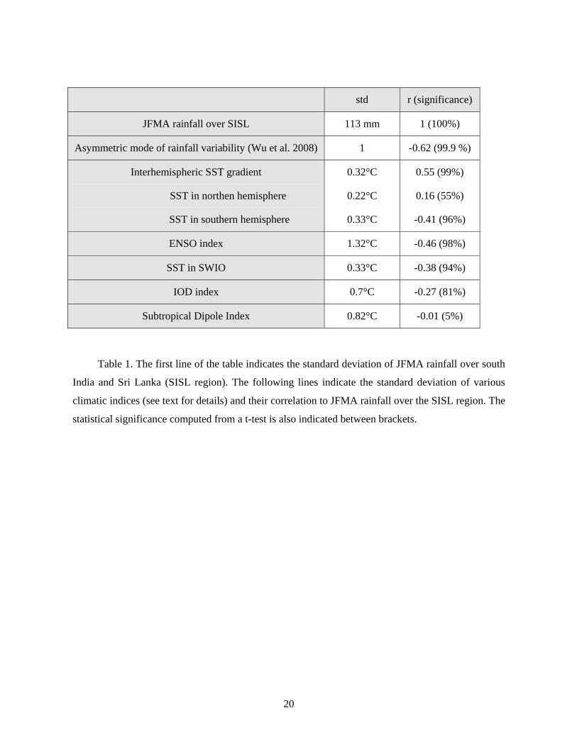
Table 1. The first line of the table indicates the standard deviation of JFMA rainfall over south

India and Sri Lanka (SISL region). The following lines indicate the standard deviation of various

climatic indices (see text for details) and their correlation to JFMA rainfall over the SISL region. The

statistical significance computed from a t-test is also indicated between brackets.

21

Figure 1. a) January-April climatological rainfall from GPCP product (contour interval 0.1 m).

b) Percentage of climatological annual rainfall falling between January and April (contour interval

5%). c) Standard-deviation of January-April interannual monthly rainfall anomalies (contour interval

0.025 m).

22

Figure 2. Map of a) March 2008 and b) April 2008 rainfall anomalies from GPCP product

(contour interval 3 mm day-1, shading for rainfall above normal), b) Map of SST anomaly for March

2008 (°C, contour interval 0.5°C, shading for negative values) from Reynolds product. The 5°N-

20°N, 70°E-85°E region, encompassing south India and Sri-Lanka is indicated for future reference.

23

Figure 3. Time series of monthly rainfall anomalies (mm day-1) over the 5°N-20°N, 70°E-85°E

region, encompassing south India and Sri-Lanka (outlined in figure 2a). A shading highlights the

January-April period and a black disk indicates the March 2008 rainfall anomaly.

24

Figure 4. a) Climatological (dashed line) and late 2007-early 2008 meridional temperature

gradient over the central and eastern Indian Ocean. The meridional temperature gradient is computed

as SST in 70°E-95°E, 3°N-10°N minus the SST in 70°E-95°E, 3°S-10°S. b) Daily rainfall (mm day-

1) over southern peninsular India and Sri Lanka (region highlighted in Figure 2a) from GPCP

product. The dashed line shows the long-term climatology from the same product. The time periods

for which the Wheeler and Hendon (2004) MJO index has a larger amplitude than one and a phase 2,

3 or 4 (active MJO phase over the Indian ocean) has been highlighted with black marks on the time

axis.

25

Figure 5. Climatological rainfall from GPCP product (contour interval 2 mm day-1, shading

above 2 mm day-1) and climatological winds from Quickscat (see plot for scale) for a) June-

September (southwest monsoon), b) October-November (northeast monsoon), c) January-March, d)

April.

26

Figure 6. Empirical Orthogonal Function analysis of the 90-day low-passed filtered GPCP

rainfall anomalies for the months of a) December, b) January, c) February, d) March, e) April, and f)

May. The spatial correlation of each pattern with the pattern for the January-April rainfall average is

indicated above each plot. The normalization is the same in each plot but the unit is arbitrary.

27

Figure 7. Composite of intraseasonally filtered (10-90 days) January-March GPCP rainfall, as a

function of the phase of the Madden-Julian Oscillation, as indicated from the Wheeler and Hendon

(2004) index. a) composite for phase 3 of the MJO (one of the active phases over the Indian Ocean,

this composite is significant at the 95% level almost everywhere); b) % of chance of having rainfall

in the highest quintile; c) average composite rainfall over Southern India and Sri Lanka (box

indicated in panels a,b) as a function of the phase of the Madden-Julian Oscillation; vertical bars

indicate the 95% confidence interval.

28

Figure 8. Time series of pentad GPCP rainfall over southern India and the Bay of Bengal

(averaged over 75°E-95°E in the 10°N-12°30’N latitude band). Rain events longer than 20 days and

> 1 mm day-1 in JFM are marked by a circle. The time series here only shows 1998 to 2007 for

clarity, but a total of25 cases between 1979 and 2007 were selected to construct the composite of

figure 9.

29

Figure 9. Composite of intraseasonally filtered (10-90 days) January-March GPCP rainfall,

averaged between 10°N-10°S and plotted as a function of time lag (in days). Lag 0 corresponds to

the 25 rainfall events over southern India shown in figure 8. The contour shows area where the signal

is significant at the 95% confidence level. The dotted line indicates 5 m.s-1 eastward propagation (the

average speed of the MJO).

30

Figure 10. a) Regression of seasonal January-April SST anomalies with interannual anomalies of

January-April rainfall over land in south peninsular India, south of 12°N (the contour interval is .1

°C with dashed contours for negative values; the shading shows area where the regression coefficient

is significantly different from zero at the 95% confidence level). The IMD gridded rainfall product

was used, but similar results are obtained with GPCP over the SISL region). b) Regression of

seasonal January-April SST anomalies with average Nino3.4 (region outlined in panel b) SST

anomalies during previous December (the contour interval is .2°C with dashed contours for negative

values; the shading shows area where the regression coefficient is significantly different from zero at

the 95% confidence level). Both regressions are performed over the 1982-2007 period with respect to

normalized indices (of standard deviation equal to 1). The sign of the regression in panel b has been

changed in order to allow an easier comparison with figure a. The Nino34 region (120°W-170°W,

5°N-5°S) is indicated on panel b.

31

Figure 11. Maps of linear regression of seasonal rainfall with El Niño (contours every .2 mm day-1

with dashed contours for negative values, i.e. decreased precipitations during an El Niño; the shading

shows area where the regression coefficient is significantly different from zero at the 95%

confidence level), a) June-September (before El Niño peak) b) October-November (before El Niño

peak), c) January-April (just after El Niño peak), d) June-September (after El Niño peak). The

regression is performed with respect to the normalized (standard deviation equal to 1) December

Niño3.4 SST anomaly. The 72°E-82°30’E, 5°N-12°30’N region encompassing South India and Sri

Lanka is indicated for future reference.

32

Figure 12. a) Time series of the regression coefficient (mm day-1 °C-1) between monthly seasonal

GPCP rainfall over the 72°E-82°30’E, 5°N-12°30’N region encompassing South India and Sri Lanka

(outlined in fig 8) and El Niño. The regression is performed with respect to the normalized (standard

deviation equal to 1) December Niño3.4 SST anomaly. b) Time series of rainfall (mm day-1)

climatology over the same region with shading showing +/- one standard deviation of seasonal

rainfall. The monthly seasonal rainfall anomaly is estimated as the monthly average of 90 day low-

passed filter daily rainfall anomalies with respect to the mean seasonal cycle.

33

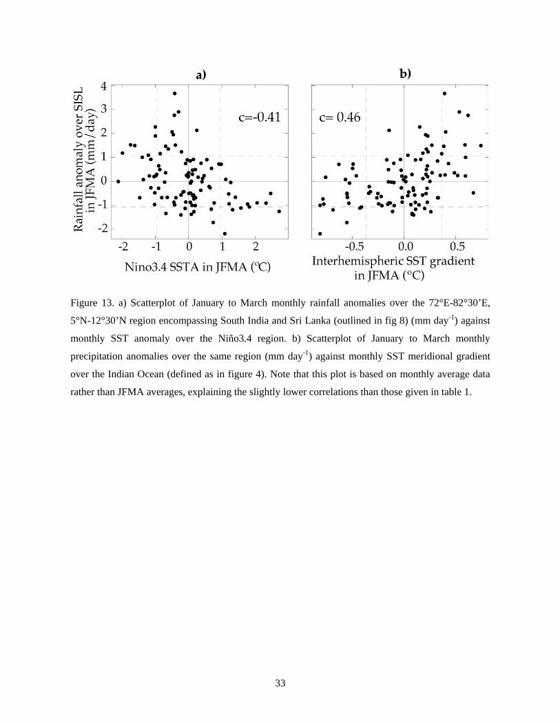
Figure 13. a) Scatterplot of January to March monthly rainfall anomalies over the 72°E-82°30’E,

5°N-12°30’N region encompassing South India and Sri Lanka (outlined in fig 8) (mm day-1) against

monthly SST anomaly over the Niño3.4 region. b) Scatterplot of January to March monthly

precipitation anomalies over the same region (mm day-1) against monthly SST meridional gradient

over the Indian Ocean (defined as in figure 4). Note that this plot is based on monthly average data

rather than JFMA averages, explaining the slightly lower correlations than those given in table 1.

34

Figure 14. Map of linear regression of January-April (just after El Niño peak) velocity potential

seasonal anomalies at 200 hPa (a proxy for the Walker circulation) with respect to normalized

Nino3.4 SST anomalies in December (contours every .25 m2 s-1 with dashed contours for negative

values, i.e. decreased precipitations during an El Niño; the shading shows area where the regression

coefficient is significantly different from zero at the 95% confidence level).