factors effecting systematic risk in isolation vs. pooled...
TRANSCRIPT
287
International Journal of Academic Research in Accounting, Finance and Management Sciences Vol. 6, No. 4, October 2016, pp. 287–300
E-ISSN: 2225-8329, P-ISSN: 2308-0337 © 2016 HRMARS
www.hrmars.com
Factors Effecting Systematic Risk in Isolation vs. Pooled Estimation:
Empirical Evidence from Banking, Insurance, and Non-Financial Sectors of Pakistan
Muhammad Nasir SHARIF1 Kashif HAMID2
Muhammad Usman KHURRAM3 Muhammad ZULFIQAR4
1Riphah International University, Faisalabad, Pakistan
2Institute of Business Management Science, University of Agriculture, Faisalabad, Pakistan,
2E-mail: [email protected] (Corresponding author)
3LSCS, University of Agriculture, Faisalabad, Pakistan,
3E-mail: [email protected]
4Government College of Commerce, Faisalabad, Pakistan
Abstract The basic purpose of the financial manager is to maximize the wealth of shareholder by minimizing the
risk. This study examines the validity of systematic risk determinants in banking, insurance, and non-financial sectors of Pakistan. Panel data is used for the period of 2010 to 2014. Common Effect Model, Generalized Method of Moments and Two step regression model is used to identify the impact. Common effect results identify that leverage; operating efficiency, firm size, and market value of equity have significant impact on systematic risk in the banking sector. Firm size has significant impact on insurance sector, whereas liquidity, leverage, operating efficiency, firm size, market value of equity, profitability, and dividend pay-out are significant variables in the non-financial sector. In pooled data analysis leverage, firm size, market value of equity, and dividend pay-out are significant determinants in Common Effect Model and Two Step, However in GMM indicates that profitability has also positive impact on unsystematic risk in addition to Common effect and two step regression determinants. Policy implication indicates that shareholders and investors can maximize the return at low level of risk by investing in selected portfolios. It is finally concluded that variables significance changes from sector to sector in individual spectrum but in a pooled regression leverage and market value of equity has negative impact on systematic risk, whereas firm size, profitability and dividend pay-out has positive impact on systematic risk.
Key words Systematic risk, common effect model, GMM, two step regression, leverage, operating efficiency
DOI: 10.6007/IJARAFMS/v6-i4/2430 URL: http://dx.doi.org/10.6007/IJARAFMS/v6-i4/2430
1. Introduction
The basic purpose of the financial manager is to maximize the wealth of shareholders. Every investor, shareholder is desirous to maximize the utility of wealth via maximizing the stock returns at a minimum level of risk. Risk is referred as volatility of a particular security. However risk of an investment refers to the actual return different from expected. More deviate return of investment from the expected return faces more risk. Risk and return relationship is established by CAPM Sharp (1964). CAPM shows that systematic risk (β) is directly proportional to the cost of equity or required rate of return. It is the best indication that factors influence systematic risk may also influence the cost of equity and ultimately firm value as well. CAPM helps in measuring portfolio risk and the expected return associated with that risk (Al-Qaisi, 2011).
Pakistan is a developing country and due to political, economic, and environmental instability investor hesitates to take investment in the firms. They are unwilling to invest the money in the highly risky securities. One factor which is related to investment is risk that is positively correlated with profit of any organization. Two types of risk exist in every organization first is systematic risk which is uncontrollable, undiversified, and market specific risk measured by equity beta and second is unsystematic risk which is controllable or diversifiable risk. Investor can avoid or minimize unsystematic risk through diversification or
International Journal of Academic Research in Accounting, Finance and Management Sciences Vol. 6 (4), pp. 287–300, © 2016 HRMARS
288
investment in portfolio. Eldomiaty et al. (2009) systematic risk is well acknowledged measure of financial risk which is dignified by beta. Value of shareholders depends upon risk of the company which decrease or increase stock prices that ultimate effect value of shareholders. Beta creates link between stock market and firm financial decision. When an investor make wrong financial decision beyond investor’s expectations so it will effect stock value negatively and as a result stock value decline which effect beta of firm. Decision making related to financing is important for managers, directors, stake holders and other financing institutions. For managers and directors low cost, low risk and higher profitability with long term capital sources is much attractive while for stakeholders and financiers attract more profit at less risk. This indicates researcher’s interest in systematic risk. This study concerned about systematic risk, market risk or external risk which is taking by investors. Beta has two ways to represent first is assets beta and second is equity beta. Assets beta represents the beta related to business risk while equity beta comprises of business risk as well as financial risk faced by shareholders. Present study is empirically examining the relationship between eight financial determinants of systematic risk as exposed by other studies, i.e. liquidity, leverage, growth, operating efficiency, firm size, market value of equity, profitability, and dividend pay-out from banking, insurance, and non-financial sectors of Pakistan. The purpose of this study is to empirically examine the determinants of systematic risk through modern evaluation techniques to further expose the factor affecting the systematic risk.
Number of studies has tested individual sector for determinants of systematic risk but this study capture the financial and non-financial sector and makes their comparison regarding to the factors associated to beta. This research considers banking, insurance and non-financial sectors of Pakistan for analysis which is still gap in the previous studies regarding to Pakistan.
This study will contribute comprehensive and knowledgeable element to the financial literature in academic and professional field and will be helpful to the investor at the time of investment, who is willing to minimize the utility by increasing the return as well as pull to policy makers who are willing raise the profitability and efficiency of the firm so that more investor attract toward investment in that company. Financial managers used this study at the time of capital budgeting to accept higher returnable projects to increase the shareholder’s wealth.
2. Literature review
Table 1. Summary of the Literature Review for Determinant of Systemic Risk
Determinants of systematic risk
Theory/Hypothesis Examples
Liquidity
Liquidity almostly have negative significant association with systematic Risk if there is no crises period.
Iqbal et al. (2015), Kerstetter (2015), Liu and Lin (2015) are agreed to this hypothesis. Li and Purice (2016) donot agreed to this hypothesis.
Leverage
Leverage have significant positive impact on systematic risk either crises exist or not
Ibrahim and Haron (2016), Li and Purice (2016), Tan et al. (2015), Liu and Lin (2015) are agreed to this hypothesis. Iqbal et al. (2015), Lee et al. (2015), Adhikari (2015) donot agreed to this hypothesis.
Growth
Growth has insignificant association with beta.
Li and Purice (2016), Adhikari (2015) and Liu and Lin (2015) are agreed to this hypothesis.
Operating Efficiency
operating efficiency is significantly negative associated with beta
Li and Purice (2016), Liu and Lin (2015) are agreed to this hypothesis. Iqbal et al. (2015), Adhikari (2015) donot agreed to this hypothesis.
Firm Size
company size has significant positive associated with beta
Li and Purice (2016), Adhikari (2015), Liu and Lin (2015) are agreed to this hypothesis.
International Journal of Academic Research in Accounting, Finance and Management Sciences Vol. 6 (4), pp. 287–300, © 2016 HRMARS
289
Hypothesis of the Study
H1: Liquidity is negatively associated with systematic risk and has significant negative Impact on systematic risk
H2: Leverage has statistically significant positive influence over systematic risk H3: Growth has significantly negative impact on systematic risk H4: Operating efficiency has negative influence over systematic risk H5: Firm size has significant positive effect on systematic risk H6: Market value of equity is significant negative associated with systematic risk H7: Profitability has significant positive influence over systematic risk H8: Dividend pay-out has significant negative influence on systematic risk
3. Methodology of research
3.1. Research design
The methodology examines the impact of determinants on systematic risk. Beta = f(LIQ, LEV, GH, OE, FS, MVE , P, DP) (1) Whereas: LIQ = Liquidity; LEV = Leverage; GH = Growth; OE = Operating Efficiency; FS = Firm Size; MVE = Market value of Equity; P = Profitability; DP = Dividend Policy.
(2) The general estimation equation is narrated as below for the above function.
(3) 1. j = number of firms in each group (banks, insurance, non-financial). 2. t = time (annual data).
3. = The constant of the regression equation
4. = The independent variables (fundamental financial ratios)
5. = The coefficient of the independent variables
6. = The error term of the regression equation.
Iqbal et al. (2015), Lee et al. (2015) do not agreed to this hypothesis.
Market Value of Equity
Negative relationship between market value of equity and beta.
Iqbal and Shah (2012) are agreed to this hypothesis. Ahmad et al. (2011) donot agreed to this hypothesis.
Profitability
profitability is significant negatively associated with beta
Li and Purice (2016), Liu and Lin (2015), Lee et al. (2015) are agreed to this hypothesis. Iqbal et al. (2015), Adhikari (2015) donot agreed to this hypothesis.
Dividend Payout Dividend has significant negative impact on systemic risk which is measured.
Adhikari (2015) and Jiao (2013) are agreed to this hypothesis.

International Journal of Academic Research in Accounting, Finance and Management Sciences Vol. 6 (4), pp. 287–300, © 2016 HRMARS
290
Common Effect Model, Generalized Methods of Moment and Two Step Regression is used to compute the sectoral comparative and pooled results.
4. Findings and discussions
Table 1 shows that mean value of beta is 1.15 which means banking stocks are more volatile than market index. It also indicates that selected companies are more riskier than market. Quick assets are 10 percent of the total assets to pay its short term obligation. Total debt to total assets ratio is 0.89 which means debt is 89.10 percent of total assets which shows that Pakistani banks more assets are financed with debt. Growth has mean value 0.20. Operating efficiency has the mean value of 0.08 and have probability value is 0.29 which shows banks total assets generate 8.23 percent revenue. Mean value of profitability is 0.02 having probability value is 0.94 which describe that banks total assets generate 1.90 percent income. Firm size, market value of equity and dividend pay-out means is 20.67, 4.66 and 0.56 having probability value is 0.75, 0.52, and 0.53 respectively.
Table 1. Descriptive Statistics of Banking Sector
BETA LIQ LEV G OE FS MVE PROF DP
Mean 1.15 0.10 0.89 0.20 0.08 20.67 4.66 0.02 0.56
Median 1.18 0.11 0.89 0.16 0.08 20.66 4.66 0.02 0.65
Maximum 1.30 0.14 0.92 2.27 0.10 21.35 5.72 0.03 1.40
Minimum 0.86 0.05 0.86 -0.68 0.07 19.92 3.71 0.00 0.00
Std. Dev. 0.15 0.03 0.02 0.48 0.01 0.38 0.57 0.01 0.45
Skewness -1.13 -0.09 -0.34 3.06 0.75 -0.04 0.25 -0.06 0.15
Kurtosis 2.83 1.50 1.97 15.10 2.59 2.27 2.00 3.33 1.93
Jarque-Bera 5.34 2.38 1.58 191.41 2.50 0.56 1.31 0.13 1.28
Probability 0.07 0.30 0.45 0.00 0.29 0.75 0.52 0.94 0.53
Sum 28.73 2.50 22.28 4.99 2.06 516.77 116.47 0.47 13.89
Sum Sq. Dev. 0.57 0.02 0.01 5.59 0.00 3.44 7.91 0.00 4.94
Observations 25 25 25 25 25 25 25 25 25
Table 2 indicates that beta is only significantly positively correlated with dividend pay-out ratio but
significantly negatively associated with liquidity, leverage, firm size and market value of equity. As the series have no multicollinearity and all independent variable are independent from one another so we can say that there is no multicollinear effect. However leverage has negative significant association with profitability and market value of the firm.
Table 2. Correlation Matrix of Banking Sector
BETA LIQ LEV OE PROF FS G DP MVE
BETA 1 LIQ -0.149 1
LEV -0.407 0.120 1 OE 0.079 -0.177 -0.234 1
PROF 0.068 -0.491 -0.504 0.542 1 FS -0.371 0.468 0.090 -0.752 -0.572 1
G 0.034 -0.264 -0.019 -0.002 -0.066 0.137 1 DP 0.117 0.046 -0.371 0.427 0.629 -0.452 -0.195 1
MVE -0.313 -0.422 -0.410 -0.083 0.623 0.079 -0.054 0.189 1
Table 3 Common effect model shows that leverage, operating efficiency, firm size, and market value
of equity are significant at p<0.05 and adjusted R2 is 0.689 which shows that shared variance of independent variables. Independent variables explain 68.9% to dependent variable. Liquidity, profitability, growth, and dividend pay-out are found to be insignificant variables in the model.

International Journal of Academic Research in Accounting, Finance and Management Sciences Vol. 6 (4), pp. 287–300, © 2016 HRMARS
291
Table 3. Common Effect Model of Baking Sector
Variables Coefficient Std. Error t-Statistic Prob.
C 15.638 2.950 5.302 0.000
LIQ 0.316 1.181 0.267 0.793
LEV -5.767 1.038 -5.557 0.000*
OE -13.761 3.443 -3.997 0.001*
PROF 7.031 8.403 0.837 0.415
FS -0.359 0.127 -2.839 0.012*
G 0.029 0.046 0.632 0.536
DP -0.074 0.066 -1.123 0.278
MVE -0.197 0.067 -2.943 0.010*
R-squared 0.793 Mean dependent var
1.149
Adjusted R-squared 0.689 S.D. dependent var
0.154
S.E. of regression 0.086 Akaike info criterion
-1.795
Sum squared resid 0.118 Schwarz criterion
-1.356
Log likelihood 31.438 Hannan-Quinn criter.
-1.673
F-statistic 7.642 Durbin-Watson stat
0.758
Prob(F-statistic) 0.000
Significant at 0.05*
Significant at 0.10**
Table 4 shows the result of variance inflation factors to check the multicollinearity. Liquidity,
leverage, Growth, operating efficiency, firm size, market value of equity, profitability, and dividend pay-out and have centered variance inflation factors 4.238, 1.522, 1.619, 3.675, 7.46, 4.791, 8.202, and 2.874 respectively. All independent variables have centered value is less than 10 that represent there is no multicollinearity exist in the data.
Table 4. Variance inflation factor of baking sector
Coefficient Uncentered Centered
Variables Variance VIF VIF
C 8.701 29406.280 NA
LIQ 1.395 51.557 4.237
LEV 1.077 2891.629 1.522
OE 11.852 274.983 3.675
PROF 70.603 91.878 8.202
FS 0.016 23148.780 7.461
G 0.002 1.908 1.619
DP 0.004 7.356 2.874
MVE 0.005 333.442 4.791
Table 5 represent the heteroskedasticity test in the panel data. F statistics is 0.725 and probability
value of whole model is 0.575 and 0.944 shows that test is insignificant which elaborates that there exist no heteroskedasticity. Adjusted R2 is -0.101 and the probability value of 0.669 is also insignificant. So we accept null hypothesis that there is no heteroskedasticity exist. Probability value of all independent variables i.e. liquidity, leverage, growth, operating efficiency, firm size, profitability, firm size, growth, dividend pay-out and market value of equity is 0.157, 0.211, 0.177, 0.701, 0.180, 0.383, 0.819 and 0.423 respectively which indicates that each variable is insignificant so there is no Heteroskedasticity. Heteroskedasticity rejection improves the significance of the ordinary least square estimate.

International Journal of Academic Research in Accounting, Finance and Management Sciences Vol. 6 (4), pp. 287–300, © 2016 HRMARS
292
Table 5. Heteroskedasticity of Baking Sector
F-statistic 0.725 Prob. F(8,16) 0.669
Obs*R-squared 6.649 Prob. Chi-Square(8) 0.575
Scaled explained SS 2.847 Prob. Chi-Square(8) 0.944
Variable Coefficient Std. Error T-Statistic Prob.
C 0.207 0.251 0.823 0.423
LIQ 0.149 0.101 1.484 0.157
LEV 0.115 0.088 1.305 0.211
OE -0.414 0.293 -1.412 0.177
PROF 0.280 0.716 0.390 0.701
FS -0.015 0.011 -1.403 0.180
G 0.004 0.004 0.897 0.383
DP -0.001 0.006 -0.233 0.819
MVE 0.005 0.006 0.822 0.423
R-squared 0.266 Mean dependent var
0.005
Adjusted R-squared -0.101 S.D. dependent var
0.007
S.E. of regression 0.007 Akaike info criterion
-6.720
Sum squared resid 0.001 Schwarz criterion
-6.281
Log likelihood 92.997 Hannan-Quinn criter.
-6.598
F-statistic 0.725 Durbin-Watson stat
1.504
Prob(F-statistic) 0.668
Table 6 shows that mean value of beta is 1.02 having probability value is 0.55 which means bank
stocks are more volatile than market index. It also indicates that selected companies are more risky than market. Quick assets are 7 percent of the total assets to pay its short term obligation. Total debt to total assets ratio is 0.54 which means debt is 54 percent of total assets which shows that Pakistani insurance companies more assets are financed with debt. Growth has mean value of –0.89 having probability value is 0.00. Operating efficiency has the mean value of 0.04 having probability value is 0.68 which shows banks total assets generated 4 percent revenue. Mean value of profitability is 0.04 having probability value is 0.79 which describe that banks total assets generate 4 percent income. Firm size, dividend pay-out, and market value of equity means are 16.26, 0.3, and 4.63 having probability value is 0.03, 0.21, and 0.50 respectively.
Table 6. Descriptive statistics of insurance sector
BETA LIQ LEV G OE FS MVE PROF DP
Mean 1.02 0.07 0.54 -0.89 0.04 16.26 4.63 0.04 0.30
Median 0.91 0.07 0.53 0.35 0.04 16.97 4.53 0.03 0.28
Maximum 1.91 0.19 0.94 2.30 0.09 17.72 6.08 0.12 0.95
Minimum -0.02 0.00 0.11 -16.97 -0.01 13.36 3.62 -0.03 0.00
Std. Dev. 0.66 0.05 0.25 3.88 0.03 1.36 0.72 0.03 0.23
Skewness -0.26 0.44 0.04 -3.14 0.17 -1.28 0.26 0.33 0.76
Kurtosis 2.07 3.29 2.38 13.24 2.21 3.06 1.98 2.86 3.81
Jarque-Bera 1.18 0.88 0.41 150.23 0.78 6.83 1.38 0.47 3.12
Probability 0.55 0.64 0.82 0.00 0.68 0.03 0.50 0.79 0.21
Sum 25.57 1.84 13.46 -22.18 0.94 406.47 115.73 0.97 7.47
Sum Sq. Dev. 10.49 0.05 1.48 360.39 0.02 44.34 12.51 0.03 1.26
Observations 25.00 25.00 25.00 25.00 25.00 25.00 25.00 25.00 25.00
Table 7 shows beta is positively correlated with liquidity, leverage, firm size, and dividend pay-out
and negatively correlated with growth, operating efficiency, market value of equity, and profitability significantly.

International Journal of Academic Research in Accounting, Finance and Management Sciences Vol. 6 (4), pp. 287–300, © 2016 HRMARS
293
Table 7. Correlation matrix of insurance sector
BETA LIQ LEV G OE FS MVE PROF DP
BETA 1 LIQ 0.138 1
LEV 0.180 0.868 1 G -0.197 0.068 0.167 1
OE -0.372 -0.444 -0.606 0.008 1 FS 0.853 0.259 0.279 -0.163 -0.412 1
MVE -0.607 -0.143 -0.062 0.182 0.169 -0.479 1 PROF -0.331 -0.122 -0.115 0.362 0.695 -0.396 0.321 1
DP 0.499 0.195 0.320 0.061 -0.381 0.753 0.034 -0.210 1
Table 8 Common Effect Model elaborates that only Firm Size has positive significant impact at p<0.05. R2 is 0.829 and adjusted R2 is 0.743 which elaborates high explanation of independent variable to dependent variable.
Table 8. Common effect model of insurance sector
Variable Coefficient Std. Error t-Statistic Prob.
C -5.175 2.480 -2.086 0.053
LIQ -2.401 3.303 -0.727 0.478
LEV -0.095 0.787 -0.121 0.905
G -0.014 0.021 -0.668 0.514
OE -7.888 5.596 -1.410 0.178
FS 0.462 0.126 3.653 0.002*
MVE -0.179 0.150 -1.195 0.249
PROF 5.811 3.959 1.468 0.162
DP -0.652 0.663 -0.983 0.340
R-squared 0.829 Mean dependent var
1.023
Adjusted R-squared 0.743 S.D. dependent var
0.661
S.E. of regression 0.335 Akaike info criterion
0.924
Sum squared resid 1.795 Schwarz criterion
1.363
Log likelihood -2.549 Hannan-Quinn criter.
1.046
F-statistic 9.693 Durbin-Watson stat
0.504
Prob (F-statistic) 0.000 Significant at 0.05*
Significant at 0.10**
Table 9 shows the result of variance inflation factors to check the multicollinearity. Liquidity, leverage, Growth, operating efficiency, firm size, market value of equity, profitability, and dividend payout and have centered variance inflation factors 5.105, 8.176, 1.413, 5.485, 6.320, 2.512, 3.978, and 4.955 respectively. All independent variables have centered value is less than 10 which represents that there is no multicollinearity exist in the data.
Table 9. Variance Inflation Factor of Insurance Sector
Coefficient Uncentered Centered
Variables Variance VIF VIF
C 6.152 1371.021 NA
LIQ 10.913 18.339 5.105
LEV 0.619 48.182 8.176
G 0.000 1.490 1.413
OE 31.311 15.318 5.485
FS 0.016 948.341 6.320
MVE 0.023 110.046 2.512
PROF 15.676 9.217 3.978
DP 0.440 13.701 4.955
International Journal of Academic Research in Accounting, Finance and Management Sciences Vol. 6 (4), pp. 287–300, © 2016 HRMARS
294
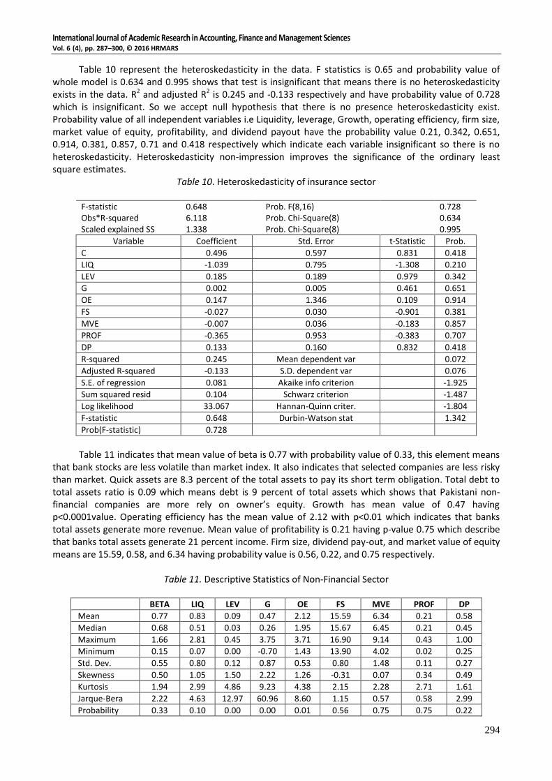
Table 10 represent the heteroskedasticity in the data. F statistics is 0.65 and probability value of whole model is 0.634 and 0.995 shows that test is insignificant that means there is no heteroskedasticity exists in the data. R2 and adjusted R2 is 0.245 and -0.133 respectively and have probability value of 0.728 which is insignificant. So we accept null hypothesis that there is no presence heteroskedasticity exist. Probability value of all independent variables i.e Liquidity, leverage, Growth, operating efficiency, firm size, market value of equity, profitability, and dividend payout have the probability value 0.21, 0.342, 0.651, 0.914, 0.381, 0.857, 0.71 and 0.418 respectively which indicate each variable insignificant so there is no heteroskedasticity. Heteroskedasticity non-impression improves the significance of the ordinary least square estimates.
Table 10. Heteroskedasticity of insurance sector
F-statistic 0.648 Prob. F(8,16) 0.728 Obs*R-squared 6.118 Prob. Chi-Square(8) 0.634 Scaled explained SS 1.338 Prob. Chi-Square(8) 0.995
Variable Coefficient Std. Error t-Statistic Prob.
C 0.496 0.597 0.831 0.418
LIQ -1.039 0.795 -1.308 0.210
LEV 0.185 0.189 0.979 0.342
G 0.002 0.005 0.461 0.651
OE 0.147 1.346 0.109 0.914
FS -0.027 0.030 -0.901 0.381
MVE -0.007 0.036 -0.183 0.857
PROF -0.365 0.953 -0.383 0.707
DP 0.133 0.160 0.832 0.418
R-squared 0.245 Mean dependent var
0.072
Adjusted R-squared -0.133 S.D. dependent var
0.076
S.E. of regression 0.081 Akaike info criterion
-1.925
Sum squared resid 0.104 Schwarz criterion
-1.487
Log likelihood 33.067 Hannan-Quinn criter.
-1.804
F-statistic 0.648 Durbin-Watson stat
1.342
Prob(F-statistic) 0.728
Table 11 indicates that mean value of beta is 0.77 with probability value of 0.33, this element means that bank stocks are less volatile than market index. It also indicates that selected companies are less risky than market. Quick assets are 8.3 percent of the total assets to pay its short term obligation. Total debt to total assets ratio is 0.09 which means debt is 9 percent of total assets which shows that Pakistani non-financial companies are more rely on owner’s equity. Growth has mean value of 0.47 having p<0.0001value. Operating efficiency has the mean value of 2.12 with p<0.01 which indicates that banks total assets generate more revenue. Mean value of profitability is 0.21 having p-value 0.75 which describe that banks total assets generate 21 percent income. Firm size, dividend pay-out, and market value of equity means are 15.59, 0.58, and 6.34 having probability value is 0.56, 0.22, and 0.75 respectively.
Table 11. Descriptive Statistics of Non-Financial Sector
BETA LIQ LEV G OE FS MVE PROF DP
Mean 0.77 0.83 0.09 0.47 2.12 15.59 6.34 0.21 0.58
Median 0.68 0.51 0.03 0.26 1.95 15.67 6.45 0.21 0.45
Maximum 1.66 2.81 0.45 3.75 3.71 16.90 9.14 0.43 1.00
Minimum 0.15 0.07 0.00 -0.70 1.43 13.90 4.02 0.02 0.25
Std. Dev. 0.55 0.80 0.12 0.87 0.53 0.80 1.48 0.11 0.27
Skewness 0.50 1.05 1.50 2.22 1.26 -0.31 0.07 0.34 0.49
Kurtosis 1.94 2.99 4.86 9.23 4.38 2.15 2.28 2.71 1.61
Jarque-Bera 2.22 4.63 12.97 60.96 8.60 1.15 0.57 0.58 2.99
Probability 0.33 0.10 0.00 0.00 0.01 0.56 0.75 0.75 0.22
International Journal of Academic Research in Accounting, Finance and Management Sciences Vol. 6 (4), pp. 287–300, © 2016 HRMARS
295
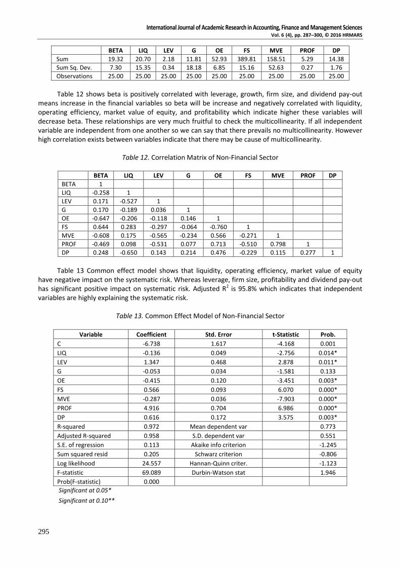
BETA LIQ LEV G OE FS MVE PROF DP
Sum 19.32 20.70 2.18 11.81 52.93 389.81 158.51 5.29 14.38
Sum Sq. Dev. 7.30 15.35 0.34 18.18 6.85 15.16 52.63 0.27 1.76
Observations 25.00 25.00 25.00 25.00 25.00 25.00 25.00 25.00 25.00
Table 12 shows beta is positively correlated with leverage, growth, firm size, and dividend pay-out
means increase in the financial variables so beta will be increase and negatively correlated with liquidity, operating efficiency, market value of equity, and profitability which indicate higher these variables will decrease beta. These relationships are very much fruitful to check the multicollinearity. If all independent variable are independent from one another so we can say that there prevails no multicollinearity. However high correlation exists between variables indicate that there may be cause of multicollinearity.
Table 12. Correlation Matrix of Non-Financial Sector
BETA LIQ LEV G OE FS MVE PROF DP
BETA 1 LIQ -0.258 1
LEV 0.171 -0.527 1 G 0.170 -0.189 0.036 1
OE -0.647 -0.206 -0.118 0.146 1 FS 0.644 0.283 -0.297 -0.064 -0.760 1
MVE -0.608 0.175 -0.565 -0.234 0.566 -0.271 1 PROF -0.469 0.098 -0.531 0.077 0.713 -0.510 0.798 1
DP 0.248 -0.650 0.143 0.214 0.476 -0.229 0.115 0.277 1
Table 13 Common effect model shows that liquidity, operating efficiency, market value of equity
have negative impact on the systematic risk. Whereas leverage, firm size, profitability and dividend pay-out has significant positive impact on systematic risk. Adjusted R2 is 95.8% which indicates that independent variables are highly explaining the systematic risk.
Table 13. Common Effect Model of Non-Financial Sector
Variable Coefficient Std. Error t-Statistic Prob.
C -6.738 1.617 -4.168 0.001
LIQ -0.136 0.049 -2.756 0.014*
LEV 1.347 0.468 2.878 0.011*
G -0.053 0.034 -1.581 0.133
OE -0.415 0.120 -3.451 0.003*
FS 0.566 0.093 6.070 0.000*
MVE -0.287 0.036 -7.903 0.000*
PROF 4.916 0.704 6.986 0.000*
DP 0.616 0.172 3.575 0.003*
R-squared 0.972 Mean dependent var
0.773
Adjusted R-squared 0.958 S.D. dependent var
0.551
S.E. of regression 0.113 Akaike info criterion
-1.245
Sum squared resid 0.205 Schwarz criterion
-0.806
Log likelihood 24.557 Hannan-Quinn criter.
-1.123
F-statistic 69.089 Durbin-Watson stat
1.946
Prob(F-statistic) 0.000 Significant at 0.05*
Significant at 0.10**

International Journal of Academic Research in Accounting, Finance and Management Sciences Vol. 6 (4), pp. 287–300, © 2016 HRMARS
296
Table 14 shows the result of variance inflation factors to check the multicollinearity. Liquidity, leverage, Growth, operating efficiency, firm size, market value of equity, profitability, and dividend payout and have centered variance inflation factors 2.907, 5.72, 1.607, 7.705, 6.291, 5.392, 5.378, and 4.071 respectively. All independent variables have centered value is less than 10 that represent there is no multicollinearity exist in the data.
Table 14. Variance Inflation Factor of Non-Financial Sector
Coefficient Uncentered Centered
Variables Variance VIF VIF
C 2.613 5093.341 NA
LIQ 0.002 6.153 2.907
LEV 0.219 8.954 5.720
G 0.001 2.1 1.607
OE 0.014 133.794 7.704
FS 0.009 4135.136 10.291
MVE 0.001 108.371 5.392
PROF 0.495 53.533 10.379
DP 0.030 23.221 4.071
Table 15 represent the heteroskedasticity in the data. F statistics is 0.553 and probability value of
whole model is 0.738 and 0.988 shows test is insignificant that means there is no heteroskedasticity exist in the data. R2 and adjusted R2 is 0.207 and -0.189 respectively and have insignificant p-value > 0.823. So we accept null hypothesis that there prevails no heteroskedasticity. Probability value of all independent variables i.e liquidity, leverage, growth, operating efficiency, firm size, market value of equity, profitability, and dividend payout have the probability value 0.272, 0.693, 0.382, 0.648, 0.825, 0.504, 0.927, and 0.322 respectively which indicates that each variable is insignificant so there prevails no heteroskedasticity.
Table 15. Heteroskedasticity of non-financial sector
F-statistic 0.523 Prob. F(8,16) 0.823 Obs*R-squared 5.179 Prob. Chi-Square(8) 0.738
Scaled explained SS 1.725 Prob. Chi-Square(8) 0.988
Variable Coefficient Std. Error t-Statistic Prob.
C 0.063 0.166 0.378 0.710
LIQ -0.006 0.005 -1.138 0.272
LEV -0.019 0.048 -0.402 0.693
G -0.003 0.004 -0.899 0.382
OE 0.006 0.012 0.465 0.648
FS -0.002 0.01 -0.225 0.825
MVE -0.003 0.004 -0.685 0.504
PROF 0.007 0.072 0.093 0.927
DP -0.018 0.018 -1.023 0.322
R-squared 0.207 Mean dependent var
0.008
Adjusted R-squared -0.189 S.D. dependent var
0.011
S.E. of regression 0.012 Akaike info criterion
-5.793
Sum squared resid 0.002 Schwarz criterion
-5.354
Log likelihood 81.410 Hannan-Quinn criter.
-5.671
F-statistic 0.523 Durbin-Watson stat
2.612
Prob(F-statistic) 0.823
Pooled Regression
Table 16 shows the results of common effect model with pooled data which is pooled combination of all three sectors. Results predict that whole model is significant at 0.05 with four independent variables i.e.

International Journal of Academic Research in Accounting, Finance and Management Sciences Vol. 6 (4), pp. 287–300, © 2016 HRMARS
297
leverage, firm size market value of equity, and dividend pay-out. R2 is 0.569 and adjusted R2 is 0.517 which represent shared variance of independent variables that means change in dependent variable due to change in independent variables is 56.94% which represent fitness of model that more change in dependent variable is due to eight independent variables. Liquidity, growth and operating efficiency are found insignificant variables in common effect model. Profitability is significant at 0.1.
Table 16. Common effect model
Variables Coefficient Std. Error t-Statistic Prob.
C 0.541 0.497 1.087 0.281
LIQ -0.088 0.098 -0.898 0.372
LEV -0.791 0.26 -3.043 0.003*
G -0.019 0.019 -1.031 0.306
OE -0.154 0.102 -1.503 0.138
FS 0.128 0.03 4.318 0.000*
MVE -0.311 0.059 -5.241 0.000*
PROF 1.981 1.100 1.800 0.076**
DP 0.364 0.142 2.565 0.013*
R-squared 0.569 Mean dependent var 0.982
Adjusted R-squared 0.517 S.D. dependent var 0.522
S.E. of regression 0.363 Akaike info criterion 0.924
Sum squared resid 8.698 Schwarz criterion 1.202
Log likelihood -25.631 Hannan-Quinn criter. 1.035
F-statistic 10.907 Durbin-Watson stat 0.706
Prob(F-statistic) 0.000
Significant at 0.05*
Significant at 0.10**
Table 17 shows the impact of liquidity, leverage, growth, operating efficiency, firm size, and market value of equity, profitability, and dividend payout on systematic risk by using Generalized Method of Moments. Results predict that five independent variables i.e. leverage, firm size, market value of equity, profitability, and dividend pay-out are significant at p<0.05 and only one variable is significant at p<0.10. R2
is 0.546 and adjusted R2 is 0.491 which indicates the explanatory power of independent variables to dependent variable. Leverage, growth and market value of equity has negative impact on systematic risk and firm size, profitability and dividend payout has positive significant impact on systematic risk. The J statistics is less than 0.0000 which indicate that whole model is significant at p<0.05.
Table 17. Generalized Method of Moments
Variables Coefficient Std. Error T-Statistic Prob.
C 0.446 0.49 0.911 0.366
LIQ -0.034 0.091 -0.376 0.708
LEV -0.676 0.289 -2.341 0.022*
G -0.022 0.011 -1.985 0.051**
OE -0.098 0.1 -0.992 0.325
FS 0.127 0.027 4.644 0.000*
MVE -0.31 0.044 -7.109 0.000*
PROF 1.748 0.815 2.146 0.036*
DP 0.288 0.104 2.764 0.007*
R-squared 0.546 Mean dependent var 0.982
Adjusted R-squared 0.491 S.D. dependent var 0.522
S.E. of regression 0.373 Sum squared resid 9.162
Durbin-Watson stat 0.641 J-statistic 24.621
Instrument rank 10 Prob(J-statistic) 0.000
Significant at 0.05* Significant at 0.10**

International Journal of Academic Research in Accounting, Finance and Management Sciences Vol. 6 (4), pp. 287–300, © 2016 HRMARS
298
Table 18 indicates the forward step wise regression and results indicate that liquidity, market value of equity have negative impact. However firm size, profitability, and dividend pay-out has positive significant impact on systematic risk. R2 explains that 56.9% dependent variable is explained by independent variables.
Table 18. Forward Step Wise Regression
Selection method: Stepwise forwards Stopping criterion: p-value forwards/backwards = 0.5/NA
Variables Coefficient Std. Error t-Statistic Prob.
C 0.541 0.497 1.087 0.281
LIQ -0.088 0.098 -0.898 0.372
LEV -0.791 0.26 -3.043 0.003*
G -0.02 0.019 -1.031 0.306
OE -0.154 0.102 -1.503 0.138
FS 0.128 0.03 4.318 0.000*
MVE -0.310 0.059 -5.241 0.000*
PROF 1.981 1.100 1.800 0.076**
DP 0.364 0.142 2.565 0.013*
R-squared 0.569 Mean dependent var 0.982
S.D. dependent var 0.522 S.E. of regression 0.363
Akaike info criterion 0.924 Sum squared resid 8.698
Schwarz criterion 1.202 Log likelihood -25.631
Hannan-Quinn criter. 1.035 F-statistic 10.907
Durbin-Watson stat 0.706
Significant at 0.05*
Significant at 0.10**
Table 19 results indicate that leverage, market value of equity has negative impact on systematic risk
whereas firm’s size, profitability and dividend pay-out have positive impact on systematic risk by using backward step wise regression. The value of R2 indicates that 56.93% portion of dependency is explained by the independent variables.
Table 19. Backward Step Wise Regression
Selection method: Stepwise backwards Stopping criterion: p-value forwards/backwards = 0.5/NA
Variables Coefficient Std. Error T-Statistic Prob.
C 0.540739 0.497421 1.087084 0.2810
LIQ -0.088267 0.098278 -0.898134 0.3724
LEV -0.790995 0.259970 -3.042632 0.0034*
G -0.019456 0.018864 -1.031388 0.3061
OE -0.153972 0.102444 -1.502997 0.1376
FS 0.128411 0.029739 4.317932 0.0001*
MVE -0.310078 0.059161 -5.241253 0.0000*
PROF 1.980720 1.100259 1.800230 0.0764**
DP 0.363788 0.141835 2.564869 0.0126*
R-squared 0.569349 Mean dependent var 0.981672
S.D. dependent var 0.522436 S.E. of regression 0.363027
Akaike info criterion 0.923489 Sum squared resid 8.698057
Schwarz criterion 1.201587 Log likelihood -25.63082
Hannan-Quinn criter. 1.034530 F-statistic 10.90706
Durbin-Watson stat 0.705956
Significant at 0.05*
Significant at 0.10**
International Journal of Academic Research in Accounting, Finance and Management Sciences Vol. 6 (4), pp. 287–300, © 2016 HRMARS
299
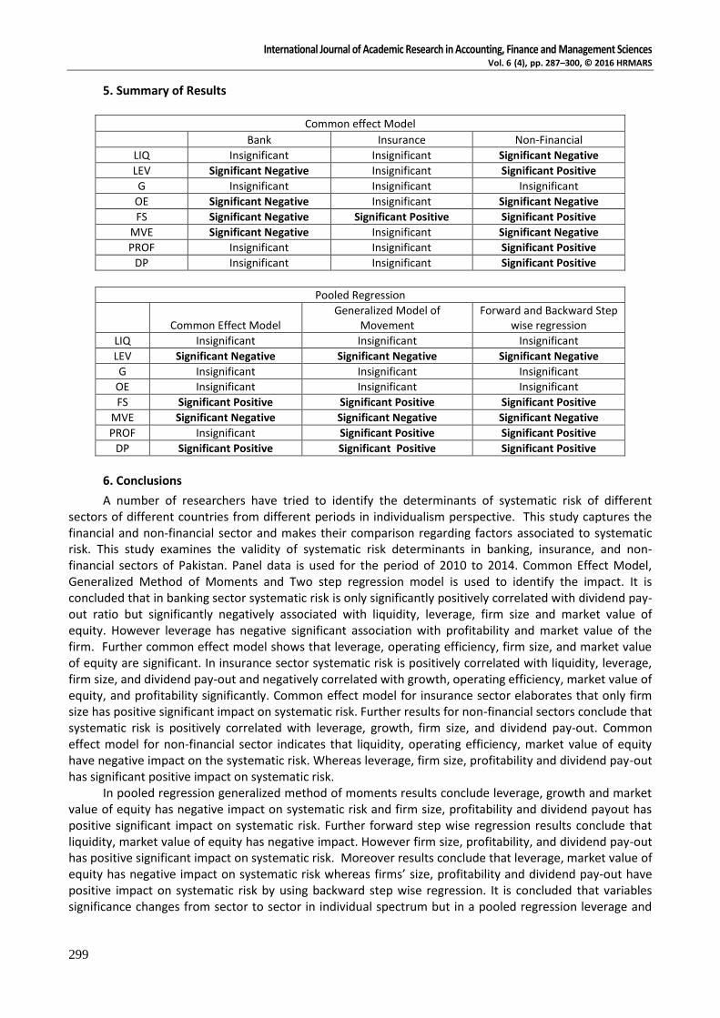
5. Summary of Results
Common effect Model
Bank Insurance Non-Financial
LIQ Insignificant Insignificant Significant Negative
LEV Significant Negative Insignificant Significant Positive
G Insignificant Insignificant Insignificant
OE Significant Negative Insignificant Significant Negative
FS Significant Negative Significant Positive Significant Positive
MVE Significant Negative Insignificant Significant Negative
PROF Insignificant Insignificant Significant Positive
DP Insignificant Insignificant Significant Positive
Pooled Regression
Common Effect Model
Generalized Model of Movement
Forward and Backward Step wise regression
LIQ Insignificant Insignificant Insignificant
LEV Significant Negative Significant Negative Significant Negative
G Insignificant Insignificant Insignificant
OE Insignificant Insignificant Insignificant
FS Significant Positive Significant Positive Significant Positive
MVE Significant Negative Significant Negative Significant Negative
PROF Insignificant Significant Positive Significant Positive
DP Significant Positive Significant Positive Significant Positive
6. Conclusions
A number of researchers have tried to identify the determinants of systematic risk of different sectors of different countries from different periods in individualism perspective. This study captures the financial and non-financial sector and makes their comparison regarding factors associated to systematic risk. This study examines the validity of systematic risk determinants in banking, insurance, and non-financial sectors of Pakistan. Panel data is used for the period of 2010 to 2014. Common Effect Model, Generalized Method of Moments and Two step regression model is used to identify the impact. It is concluded that in banking sector systematic risk is only significantly positively correlated with dividend pay-out ratio but significantly negatively associated with liquidity, leverage, firm size and market value of equity. However leverage has negative significant association with profitability and market value of the firm. Further common effect model shows that leverage, operating efficiency, firm size, and market value of equity are significant. In insurance sector systematic risk is positively correlated with liquidity, leverage, firm size, and dividend pay-out and negatively correlated with growth, operating efficiency, market value of equity, and profitability significantly. Common effect model for insurance sector elaborates that only firm size has positive significant impact on systematic risk. Further results for non-financial sectors conclude that systematic risk is positively correlated with leverage, growth, firm size, and dividend pay-out. Common effect model for non-financial sector indicates that liquidity, operating efficiency, market value of equity have negative impact on the systematic risk. Whereas leverage, firm size, profitability and dividend pay-out has significant positive impact on systematic risk.
In pooled regression generalized method of moments results conclude leverage, growth and market value of equity has negative impact on systematic risk and firm size, profitability and dividend payout has positive significant impact on systematic risk. Further forward step wise regression results conclude that liquidity, market value of equity has negative impact. However firm size, profitability, and dividend pay-out has positive significant impact on systematic risk. Moreover results conclude that leverage, market value of equity has negative impact on systematic risk whereas firms’ size, profitability and dividend pay-out have positive impact on systematic risk by using backward step wise regression. It is concluded that variables significance changes from sector to sector in individual spectrum but in a pooled regression leverage and

International Journal of Academic Research in Accounting, Finance and Management Sciences Vol. 6 (4), pp. 287–300, © 2016 HRMARS
300
market value of equity has negative impact on systematic risk and firm size, profitability and dividend payout has positive impact on systematic risk.
The limitation of the study is its sample size and accuracy of the available data and convenient sampling is used in this study that is not applied at whole population. Future research can be performed in the different markets perhaps in the Asian market with different modern techniques applicable for analysis of the data and large sample size can be used to generalize at whole population.
References
1. Ahmad, F., Ali, M., Arshad, M. U., and Shah, S.Z.A. (2011). Corporate tax rate as a determinant of systematic risk: Evidence from Pakistani cement sector. African Journal of Business Management, 5(33), 12762-12767.
2. Al-Qaisi, K.M. (2011). The Economic Determinants of Systematic Risk in the Jordanian Capital Market. International Journal of Business and Social Science, 2(20), 85-95.
3. Eldomiaty, T.I., Al Dhaheri, M.H., and Al Shukri, M. (2009). The Fundamental Determinants of Systematic Risk and Financial Transparency in the DFM General Index. Middle Eastern Finance and Economics, (5), 49-61.
4. Ibrahim, K., and Haron, R. (2016). Examining systematic risk on Malaysian firms: panel data evidence. Education Knowledge and Economy, 1(2), 26-30.
5. Iqbal, M.J., and Shah, S.Z.A. (2012). Determinants of systematic risk. The Journal of Commerce, 4(1), 47-56.
6. Jiao, D. (2013). Demand volatility, operating leverage and systematic risk in hospitality industry. Universiteit van Tilburg.
7. Lee, W.S., Moon, J., Lee, S., and Kerstetter, D. (2015). Determinants of systematic risk in the online travel agency industry. Tourism Economics, 21(2), 341-355.
8. Liu, D.Y., and Lin, C.H. (2015). Does Financial Crisis Matter? Systematic Risk in the Casino Industry. Journal of Global Business Management, 11(1).
9. Sharpe, W.F. (1964). Capital asset prices: A theory of market equilibrium under conditions of risk. The journal of finance, 19(3), 425-442.
10. Tan, N., Chua, J., and Salamanca, P. (2015). Study of the Overall Impact of Financial Leverage and Other Determinants of Systematic Risk. DLSU Research Congress, De La Salle University, Manila, Philippines.