Working Paper 1907 September 2019 (revised December 2020) Research Department https://doi.org/10.24149/wp1907r1

Working papers from the Federal Reserve Bank of Dallas are preliminary drafts circulated for professional comment. The views in this paper are those of the authors and do not necessarily reflect the views of the Federal Reserve Bank of Dallas or the Federal Reserve System. Any errors or omissions are the responsibility of the authors.

Facts and Fiction in Oil Market Modeling

Lutz Kilian

Facts and Fiction in Oil Market Modeling*

Lutz Kilian†

September 4, 2019 Revised: December 10, 2020

Abstract A series of recent articles has called into question the validity of VAR models of the global market for crude oil. These studies seek to replace existing oil market models by structural VAR models of their own based on different data, different identifying assumptions, and a different econometric approach. Their main aim has been to revise the consensus in the literature that oil demand shocks are a more important determinant of oil price fluctuations than oil supply shocks. Substantial progress has been made in recent years in sorting out the pros and cons of the underlying econometric methodologies and data in this debate, and in separating claims that are supported by empirical evidence from claims that are not. The purpose of this paper is to take stock of the VAR literature on global oil markets and to synthesize what we have learned. Combining this evidence with new data and analysis, I make the case that the concerns regarding the existing VAR oil market literature have been overstated and that the results from these models are quite robust to changes in the model specification. JEL Codes: Q43, Q41, C36, C52 Keywords: Elasticity, structural VAR, Bayesian inference, oil price, global real activity, oil inventories.

*Acknowledgments: The views expressed in this paper are my own and should not be interpreted as reflecting the views of the Federal Reserve Bank of Dallas or any other member of the Federal Reserve System. I thank Ron Alquist, Brian Prest, Ana Maria Herrera, Atsushi Inoue, and Xiaoqing Zhou for helpful discussions. This paper is a substantially rewritten version of an earlier paper with the same title. The author has no conflict of interest to declare. †Lutz Kilian, Federal Reserve Bank of Dallas, Research Department, 2200 N. Pearl St., Dallas, TX 75201, USA. E-mail: lkilian2019@gmail.com.

1  

1. Introduction

In a series of articles, Baumeister and Hamilton (2019a,b; 2020a) and Hamilton (2019), building

on Baumeister and Hamilton (2015, 2018, 2020b), have called into question the validity of oil

market models dating from the pioneering oil market vector autoregressive (VAR) model of

Kilian (2008, 2009) to the sign-identified VAR models of Kilian and Murphy (2012, 2014) and

their extensions.1 Baumeister and Hamilton specifically attacked the credibility of the data used,

the identifying assumptions, the econometric methodology used in these studies, and the

substantive conclusions reached in this literature. They sought to replace these oil market models

by a structural VAR model of their own based on different data, different identifying

assumptions, and a different econometric approach that they consider superior.

Although their critiques also extend to other research using structural VAR models, their

main aim has been to revise the consensus in the literature that oil demand shocks are a more

important determinant of oil price fluctuations than oil supply shocks. Baumeister and Hamilton

(2019a,b; 2020a) conclude that oil supply shocks are more important drivers of the real price of

oil and that they are much more recessionary for the U.S. economy than suggested by earlier oil

market studies including Kilian (2008, 2009) and Kilian and Murphy (2014). A number of recent

studies including Herrera and Rangaraju (2020), Kilian (2019, 2020) and Kilian and Zhou (2019)

have questioned details of their analysis, noting in particular that these conclusions are highly

sensitive to a priori assumptions about what constitutes a reasonable value for the one-month

price elasticity of oil supply. There has been no comprehensive evaluation of this debate,

 1 Recent examples of applications and extensions of these models include Antolin-Diaz and Rubio-Ramirez (2018), Baumeister and Kilian (2014, 2016), Bützer, Habib, and Stracca (2016), Herrera and Rangaraju (2020), Herwartz and Plödt (2016), Inoue and Kilian (2013; 2020a,b), Juvenal and Petrella (2015), Kilian (2017), Kilian and Lee (2014), Kilian and Zhou (2020b,c), Lippi and Nobili (2012), Ludvigson, Ma and Ng (2020), Lütkepohl and Netšunajev (2014), Montiel Olea, Stock and Watson (2020), and Zhou (2020).

2  

however.

Substantial progress has been made in recent years in sorting out the pros and cons of the

underlying econometric methodologies and data, and in separating claims that are supported by

empirical evidence from claims that are not. The purpose of this paper is to take stock of the

VAR literature on global oil markets and to synthesize what we have learned. Based on new

evidence and a careful review of the underlying econometric issues, I make the case that the

concerns regarding the existing VAR oil market literature have been overstated and that the

results from these models are quite robust to changes in the model specification. The question of

how to model oil markets may seem esoteric to many economists at first, but has important

implications for how oil-importing and oil-exporting economies respond to global oil price

fluctuations and for how policymakers should respond to these oil price fluctuations. The focus

in this paper is not only on correcting important misunderstandings in the recent literature, but on

the substantive and methodological insights generated by this exchange, which are of broader

interest to applied researchers.

The remainder of this paper is organized as follows. Section 2 clarifies the econometric

foundations of conventional sign-identified oil market models and the implications of the Haar

prior for the rotation matrix for impulse response analysis. I also explain why the alternative

econometric method proposed by Baumeister and Hamilton does not address the problem of

unintentionally informative impulse response priors, I discuss the generality of their approach,

and I review under what conditions Bayes estimates and credible sets are useful summary

statistics of the impulse response posterior. Section 3 examines the specification of the oil market

models discussed in Baumeister and Hamilton (2019a, 2020a). I emphasize the role of the

market clearing condition, I explain why classical measurement error in the change in oil

3  

inventories is not a useful modeling device, I refute Baumeister and Hamilton’s claim that

existing studies have defined the price elasticities of oil demand and oil supply incorrectly, and I

discuss the pros and cons of an explicit elasticity prior. Section 4 examines Baumeister and

Hamilton’s concern that the impulse response estimates in Kilian and Murphy (2014) are not

robust and addresses their claim that this study did not employ narrative sign restrictions. Section

5 addresses Hamilton's (2019) renewed critique of the merits of the Kilian (2009) index of global

real economic activity, which is used in many oil market studies, drawing on new results in the

literature and related econometric research. Section 6 explains the main source of the substantive

disagreement between Baumeister and Hamilton (2019a, 2020a) and the existing oil market

literature. The concluding remarks are in section 7.

2. The Econometric Foundations of Sign-Identified Oil Market VAR Models

The conventional approach to estimating sign-identified VAR models, as discussed in Uhlig

(2005), Rubio-Ramirez, Waggoner and Zha (2010), Arias, Rubio-Ramirez and Waggoner (2018)

and Antolin-Diaz and Rubio-Ramirez (2018), involves specifying a Haar prior for the orthogonal

rotation matrix Q and a Gaussian-inverse Wishart prior for the parameters A and Σ of the

reduced-form VAR model, where A denotes the slope parameters and Σ is the error covariance

matrix.2 The prior for the impulse response vector ( , , )g A Q is defined implicitly by the

function ( ).g A number of recent studies have questioned the extent to which the impulse

response estimates from these models are driven by the choice of the prior for ,Q given that Q

does not enter the likelihood and its prior cannot be overruled by the data (see, e.g., Baumeister

and Hamilton 2015, 2018, 2019a; Watson 2020). Several of these studies have argued for

 2 The Haar prior is a uniform prior in the space of all orthogonal matrices .Q

4  

ignoring empirical evidence from conventional sign-identified oil market VAR models because

they see no reason for the posterior impulse response estimates and the credible sets reported in

applied work to be more plausible than the other responses in the identified set.

This view is based on analysis in Baumeister and Hamilton (2015) who claimed that the

Haar prior typically imposed for Q is unintentionally informative about the implied prior for the

structural impulse responses. The question raised by Baumeister and Hamilton is indeed an

important question for applied work, but Inoue and Kilian (2020a) show that the tools they used

to illustrate this problem are invalid.

2.1. Why the arguments in Baumeister and Hamilton (2015) are misleading

Baumeister and Hamilton (2015) proposed characterizing the impulse response prior based on

the distribution of the impulse responses conditional on the maximum likelihood estimator

(MLE) of the reduced-form parameters. This approach, however, does not make sense from a

Bayesian point of view. The impulse response prior in Bayesian analysis captures the beliefs the

researcher holds about the distribution of the impulse responses before examining the data. Since

the impulse response distribution conditional on the MLE depends on the data by construction, it

cannot be the prior, so the results derived in Baumeister and Hamilton (2015) do not address the

question of how informative conventional priors for sign-identified models are for the impulse

response prior.

One may object that the point of conditioning on the MLE is to isolate the contribution of

the prior for Q to the prior for . The problem is that this contribution cannot be isolated. If we

restrict attention to the impact responses, for example, these responses in general can be written

as products of elements of Q and elements of . By the change-of-variable method the impulse

response prior will differ from the prior for a given element in .Q Inoue and Kilian (2020a)

5  

illustrate this point and show that the analytical examples for selected impact responses

discussed in Baumeister and Hamilton (2015) are quite misleading. The actual prior tends to look

quite different from their derivations. This point generalizes to higher horizons and to joint

inference on vectors of impulse responses, which Baumeister and Hamilton do not consider.

2.2. How informative is the Haar prior?

This result leaves unanswered the original question of how widespread unintentionally

informative impulse response priors are in applied work based on oil market models and, more

importantly, to what extent these implicit impulse response priors affect posterior inference.

Baumeister and Hamilton never documented the impulse response priors in conventional oil

market VAR models nor did they provide empirical evidence for their claim that these priors

distort posterior inference. However, Inoue and Kilian (2020a) recently derived appropriate tools

to differentiate good impulse response priors from bad ones and illustrated their use in a range of

representative empirical applications. Their evidence suggests that unduly informative impulse

response priors are the exception rather than the rule.

Inoue and Kilian (2020a) show, first, that in models identified based on static sign

restrictions only, standard uniform-Gaussian inverse Wishart priors tend to imply an

uninformative prior for in the sense that the impulse response prior in the absence of sign

restrictions is centered near zero and is fairly diffuse. This result is general in that it depends only

on the prior and not on the data. Moreover, the corresponding impulse response posterior for

is driven largely by the data rather than the prior.

Second, in models with both static and dynamic sign restrictions the implied prior for

is necessarily informative. Based on the example of the Kilian and Murphy (2014) oil market

6  

VAR model, Inoue and Kilian (2020a) illustrate that even in the latter class models the prior for

need not be unintentionally informative, directly refuting Baumeister and Hamilton’s claims

about this model. Moreover, they show that in this case as well the posterior is driven largely by

the data, not by the prior. Thus, the problem with the Kilian and Murphy (2014) model asserted

by Baumeister and Hamilton (2019a, 2020a) does not exist.

2.3. Why the alternative econometric method proposed by Baumeister and Hamilton does

not address the problem of unintentionally informative impulse response priors

Moreover, unbeknownst to Baumeister and Hamilton, their proposal of postulating priors on the

structural VAR model parameters rather than on , ,A Q implies an impulse response prior of

unknown form much like the conventional approach and hence does nothing to address the

concerns raised about the conventional approach.

The reason is simple. Imposing explicit prior distributions on the parameters 0 , , pB B in

the structural VAR representation 0 1 1 .... ,t t p t p tB y B y B y w where ty denotes the 1n

vector of data and tw the 1n vector of mutually uncorrelated structural errors, as proposed by

Baumeister and Hamilton (2015), is not equivalent to specifying an explicit prior on the vector of

structural impulse responses, which is defined by the nonlinear transformation 0 ,..., .pf B B

Even if a prior on 0 , , pB B may be defended on economic grounds, after applying the change-

of-variable method, the prior on may become unintentionally informative. This conclusion

remains true, if one is specifying an additional prior on one or more elements of 10 ,B as in the oil

market model of Baumeister and Hamilton (2019) Thus, there is nothing to choose between their

approach and the conventional approach in this regard.

When evaluating the Baumeister and Hamilton (2019a) oil market model using the tools

7  

developed in Inoue and Kilian (2020a), it can be shown that the implied impulse response prior

is highly economically implausible. For example, it postulates that an exogenous increase in

global real economic activity lowers the real price of oil (see Figure 1). This pattern is clearly at

odds with conventional views about the relationship between economic expansions and the real

price of oil. The nature of this prior was neither intended by the authors nor has it been discussed

in the literature. Because Baumeister and Hamilton never derived the implied impulse response

prior, they remained unaware of how strong and economically unreasonable their prior is. In

light of this evidence, there is no support for the claim that their methodology is inherently

superior to more conventional approaches. In fact, in practice, it may be less appealing.

2.4. Should we report the Bayes estimator and joint credible sets or the identified set?

Baumeister and Hamilton suggest that researchers using conventional priors should only report

the identified set of the impulse responses rather than the Bayes estimate and credible sets. Their

point is not that there is anything wrong with reporting Bayes estimates and credible sets from an

econometric point of view. Indeed, posterior inference about is valid from a Bayesian point of

view, given any prior for Q . Their point is that constructing posterior estimates will not be

economically sensible, unless the underlying impulse response prior can be shown to be

reasonable. There is no disagreement on this point.

However, as shown by Inoue and Kilian (2020a), the priors in standard sign-identified oil

market models such as Kilian and Murphy (2014) are either uninformative or not unintentionally

informative, and, more importantly, the impulse response posterior is largely determined by the

reduced-form parameters rather than the Haar prior. This makes Baumeister and Hamilton’s

insistence on reporting only the identified set moot, unless for a specific oil market model there

is evidence that the impulse prior is unreasonable and is driving the impulse response posterior.

8  

Appropriate tools for evaluating the joint posterior distribution of the impulse responses

are readily available under a range of alternative loss functions (see Inoue and Kilian 2020b).

These tools should be applied regardless of how the prior on the model parameters is estimated.

As observed in Inoue and Kilian (2020b), the pointwise error bands reported in Baumeister and

Hamilton (2019) are invalid measures of the estimation uncertainty about the vector of impulse

responses and tend to understate the estimation uncertainty by a factor of 3 or 4.

2.5. Other limitations of Baumeister and Hamilton’s (2019a) approach

Whether we restrict elements of 0B or 10B when identifying structural VAR models in general

depends on the economic rationale of these restrictions (see Kilian and Lütkepohl 2017). The

standard approach in the oil market VAR literature has been to put sign restrictions on the

elements of 10 .B Baumeister and Hamilton (2019a, 2020a) make the case for specifying priors on

the elements of 0B instead. Contrary to their assertion, this approach is not more natural in the

context of modeling oil markets. That’s why no one has used this approach before them.

Effectively, Baumeister and Hamilton are asking applied users to abandon existing models in

favor of alternative models with priors defined over the elements of 0.B

They emphasize that their approach is perfectly general in that it accommodates priors on

both the elements of 0B and the elements of 10 .B This claim ignores the important difference

between being able to impose restrictions on some elements of 10B and being able to impose all

relevant restrictions on 10B that an applied user would have imposed in existing oil market

models. This difference is illustrated by the fact that Baumeister and Hamilton (2019a) are

unable to replicate the Kilian and Murphy (2012) oil market model within their framework. The

“replication code” for Kilian and Murphy (2012) posted on their homepage actually is not for the

9  

Kilian and Murphy (2012) model at all. It is for a different model specification that was designed

to resemble the original model specification as closely as possible using the Baumeister-

Hamilton methodology, but imposes additional restrictions that were not part of the original

model specification.

In fact, Baumeister and Hamilton (2019a, 2020a) did not even attempt to derive a prior

that captures the cross-equation restrictions embodied in the identifying assumptions of the

Kilian and Murphy (2014) oil market model, even though this exercise would have been natural

in a study questioning the econometric validity of this model. These cross-equation restrictions

arise from the fact that the impact price elasticities depend on the response of multiple variables.

The reason why Baumeister and Hamilton do not address this question is presumably that the

resulting prior would be intractable. Thus, their approach is merely one among several

approaches, rather than encompassing all other approaches.

3. The Specification of the Oil Market Models in Baumeister and Hamilton (2019)

Baumeister and Hamilton (2019a, 2020a) claim that the oil market VAR models of Kilian (2009)

and Kilian and Murphy (2012) are misleading because they imply an unrealistically large impact

price elasticity of oil demand. Much of the confusion in the arguments of Baumeister and

Hamilton relates to the role of crude oil inventories in defining the impact price elasticity of oil

demand. It is useful to elaborate on this point.

3.1. The role of the market clearing condition

Consider the three-variable monthly global oil market model of Kilian (2009) and Kilian and

Murphy (2012). Let , , ,t t t ty q a p where tq is the growth rate of global oil production, ta

is an appropriately chosen measure of global real economic activity, and tp is the log real price

10  

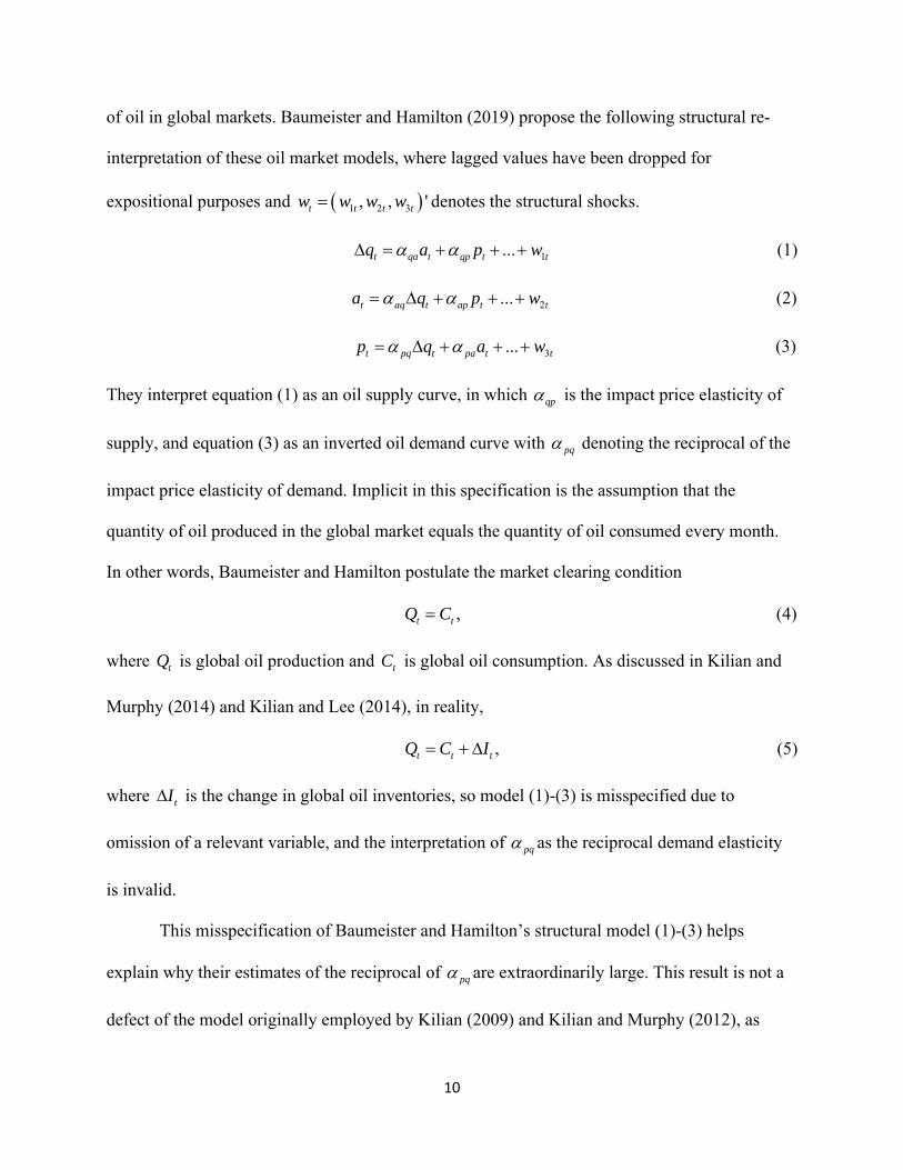
of oil in global markets. Baumeister and Hamilton (2019) propose the following structural re-

interpretation of these oil market models, where lagged values have been dropped for

expositional purposes and 1 2 3, , 't t t tw w w w denotes the structural shocks.

1...t qa t qp t tq a p w (1)

         2...t aq t ap t ta q p w (2)

          3...t pq t pa t tp q a w   (3)

They interpret equation (1) as an oil supply curve, in which qp is the impact price elasticity of

supply, and equation (3) as an inverted oil demand curve with pq denoting the reciprocal of the

impact price elasticity of demand. Implicit in this specification is the assumption that the

quantity of oil produced in the global market equals the quantity of oil consumed every month.

In other words, Baumeister and Hamilton postulate the market clearing condition

         ,t tQ C (4)

where tQ is global oil production and tC is global oil consumption. As discussed in Kilian and

Murphy (2014) and Kilian and Lee (2014), in reality,

,t t tQ C I (5)

where tI is the change in global oil inventories, so model (1)-(3) is misspecified due to

omission of a relevant variable, and the interpretation of pq as the reciprocal demand elasticity

is invalid.

This misspecification of Baumeister and Hamilton’s structural model (1)-(3) helps

explain why their estimates of the reciprocal of pq are extraordinarily large. This result is not a

defect of the model originally employed by Kilian (2009) and Kilian and Murphy (2012), as

11  

claimed by Baumeister and Hamilton. In fact, the price elasticity of oil demand is not identified

in the class of models proposed by Kilian (2009) and Kilian and Murphy (2012). Rather this

result is a defect of Baumeister and Hamilton’s alternative structural interpretation of these

models. Since similarly misspecified oil market models have been adopted in a number of other

recent oil market VAR studies including Caldara et al. (2019) and Bruns and Piffer (2019), this

point is of some importance.

Interestingly, Baumeister and Hamilton recognize the role of oil inventories in their

preferred four-variable model specification, which is re-stated below:

1...t qp t tq p w (7)

      2...t ap t ta p w   (8)

      3...t t t ca t cp t tc q i a p w   (9)

      4...t iq t ia t ip t ti q a p w .  (10)

Here 1100ln( / )t t tq Q Q is the growth rate of global oil production and 1100 /t t ti I Q

with tI denoting the change in global oil inventories, as measured in Kilian and Murphy

(2014), and tQ denoting global oil production. Baumeister and Hamilton interpret equation (9)

as an inverted oil demand curve with cp representing the impact price elasticity of oil demand.

Equivalently, equation (9) could be solved for tp , as in equation (3).3

The key assumption in this model is that t tq i is the monthly growth rate of global

oil consumption. From equation (5) we have that ,t t tC Q I so 1 1100( ) /t t t tc C C C

 3 I ignore for now the additive measurement error in ti postulated by Baumeister and Hamilton, which is

immaterial for the discussion of the identification. This point is deferred to section 3.2.

12  

1100ln( / ).t tC C It turns out that in general the correctly measured tc differs from ,t tq i as

defined in Baumeister and Hamilton (2019). Figure 2 plots a histogram of the difference between

these two variables. Baumeister and Hamilton’s monthly consumption growth measure

overstates oil consumption growth by as much as 3.3 percentage points and understates it by as

much as 4.2 percentage points. Thus, model (7)-(10) is misspecified and the implied oil demand

elasticity estimate is invalid.

3.2. Why classical additive measurement error is not the answer

One feature that sets Baumeister and Hamilton (2019) apart from other global oil market models

is their insistence on treating the change in global oil inventories as subject to measurement

error. The question here is not whether there is measurement error. There undoubtedly is error in

all observed data, including all variables in Baumeister and Hamilton’s model.4 The question is

whether this measurement error is well approximated by classical additive measurement error.

The answer is no.

In the case of global oil inventories the main concern is that the proxy for global oil

inventories proposed by Kilian and Murphy (2014) and used by Baumeister and Hamilton (2019)

excludes data from non-OECD countries. This omission matters little for much of the estimation

period, since non-OECD oil inventories traditionally have been negligible. Since some non-

OECD countries such as China have greatly increased their oil inventory holdings since the

2000s, however, one would expect this proxy to become increasingly inaccurate late in the

estimation period. Data compiled by the Energy Intelligence Group illustrate the problem.

Whereas prior to 2002 the sum of private and public crude oil stocks in China was only about

 4 The importance of measurement error in the real price of oil was emphasized in Hamilton (2011), for example, and the existence of measurement error in global oil production and global real activity is self-evident.

13  

100 million barrels, by the end of 2019, it had increased to almost 1300 million barrels (see

Figure 3).5 It follows immediately that allowing for classical measurement error in the change in

oil inventories over the entire sample will not be able to capture the systematic increases in non-

OECD oil inventories since the 2000s. Thus, Baumeister and Hamilton’s modeling approach

fails to address the root of the problem and needlessly complicates the analysis.

One solution to this problem is the use of improved global inventory data. This point was

first made in Kilian and Lee (2014) using an alternative global oil inventory series provided by

the Energy Intelligence Group (EIG). Kilian and Lee found that for their estimation period, the

estimates of the Kilian and Murphy (2014) model are remarkably similar using either oil

inventory measure. Since then EIG has developed even more accurate measures of global crude

oil inventories including Chinese commercial and strategic oil inventories that allow us to re-

examine this question. It is useful to contrast the evolution of oil stocks in OECD countries and

non-OECD countries in recent years. Figure 4 illustrates the extent to which non-OECD oil

stocks have increased relative to OECD oil stocks since 2008 in particular. It also shows an

increase in global publicly controlled strategic crude oil inventories until 2014, which mainly

reflects the creation of strategic crude oil stocks in a number of non-OECD countries (see Kilian

and Zhou 2020).

A good case can be made that in estimating global oil market models using an inventory

proxy constructed by combining the Kilian and Murphy (2014) data for the pre-1985 era with

EIG data for the more recent period, as shown in Figure 5, would be preferable to the ad hoc

assumption of additive classical measurement error, which ignores the increased importance of

non-OECD stocks in recent years. Figure 6 shows updated impulse response estimates based on

 5 In addition to commercial stocks, this estimate includes strategic crude oil stocks held by companies as well as estimates of strategic stocks controlled by the government.

14  

the same specification of the Kilian and Murphy (2014) model as in Inoue and Kilian (2020a,b),

but with the original inventory data spliced to the EIG global inventory series that starts in

1985.2. Figure 7 shows the same model estimated only on the EIG global oil inventory data since

1985.2.6 We terminate the estimation period in 2018.6 to allow direct comparisons with a

number of alternative impulse response estimates in the literature.

The impulse response estimates are not only qualitatively similar, but also similar to the

responses reported in Inoue and Kilian (2020a,b), Herrera and Rangaraju (2020), and Zhou

(2020). The main difference is that the estimation uncertainty surrounding the inventory

responses and global real activity responses is larger in Figure 6, which is to be expected given

the much shorter estimation period. The punchline is that the results from the original

specification are remarkably similar to the results based on the alternative global oil inventory

data.

Another way of assessing the effect of using the EIG’s global inventory data is to

compare the impact price elasticities of oil demand and oil supply across model specifications.

Table 1 show posterior median estimates of each of these elasticities for three model

specifications. It shows that the elasticities implied by the specifications underlying Figures 6

and 7 are virtually identical, confirming the robustness of the estimates. Compared with the

specification estimated in Inoue and Kilian (2020a,b) based on the original Kilian and Murphy

(2014) proxy for global inventories, the one-month demand elasticity drops from -0.29 to about

-0.20, while the one-month oil supply elasticity remains unchanged at -0.02. This demand

elasticity estimate is about half of state-of-the-art estimates of the one-month U.S. price elasticity

 6 In the latter case, all but one of the narrative restrictions are outside of the estimation period. We follow the recent literature in imposing additional dynamic sign restrictions. The implied level of the inventory response is assumed to be of the same sign as the impact response for the first year after a shock. For consistency, we impose the same restriction in Figure 5, although similar results are obtained on the full sample without that additional restriction.

15  

of gasoline demand (see Kilian 2020), It is also more reasonable than the estimate of -0.35

reported in Baumeister and Hamilton (2019a).

3.3. The definition of the impact price elasticities of oil supply and oil demand

Baumeister and Hamilton (2019, 2020a) insist that the impact price elasticities of oil demand and

oil supply should be defined as functions of the parameters in the matrix 0B in the structural

VAR representation 0 1 1 ... .t t p t p tB y B y B y w They point out correctly that this elasticity

definition in general differs from that underlying the work of Kilian and Murphy (2012, 2014)

and related studies.

For example, Baumeister and Hamilton define the oil supply elasticity as the impact

response of oil production to an increase in the real price of oil triggered by an exogenous

demand shift, holding constant not only the remaining structural shocks, but also all other

variables in the model such as global real economic activity and oil inventories. In contrast,

Kilian and Murphy (2014) define the one-month price elasticity of oil supply as the ratio of the

impact response of oil production to the impact response in the real price of oil triggered by an

exogenous demand shift, with all other structural shocks set to zero. This allows global real

activity and oil inventories to respond contemporaneously to the exogenous demand shift. The

latter changes in turn may affect the quantity produced. Clearly, these elasticity concepts are

neither numerically nor conceptually equivalent.7 Where Baumeister and Hamilton are clearly

mistaken, is when they claim that their approach is the only correct approach to defining oil

demand and oil supply elasticities. In fact, the approach taken in Kilian and Murphy

 7 A practical difference is that Baumeister and Hamilton’s approach ensures by construction a unique estimate of the oil supply elasticity, whereas Kilian and Murphy’s approach produces two estimates of the oil supply elasticity that need not be identical, one in response to the flow demand shock and one in response to the storage demand shock. Given that these estimates in practice tend to differ only by the second decimal point, however, there is little loss in generality in reporting an average supply elasticity estimate. 

16  

(2012, 2014) and many other studies is appropriate and internally consistent.

As discussed in Kilian (2020), either of these approaches in principle can be used to rule

out structural models that are economically implausible, provided the underlying model is

correctly specified and the elasticities are defined in an internally consistent manner. However,

whereas the implementation of Kilian and Murphy’s (2014) approach is straightforward, writing

down a correctly specified oil market model using the approach of Baumeister and Hamilton

(2019) is not, as shown in section 2. Moreover, care must be taken not to specify an

unintentionally informative impulse response prior.

Another key advantage of the approach taken by Kilian and Murphy is that their elasticity

definition corresponds to the way elasticities are typically estimated at the micro level and the

way oil supply elasticity bounds have been constructed from aggregate data, facilitating the use

of these estimates in specifying and evaluating oil market models. In contrast, these extraneous

estimates are not suitable in general for motivating elasticity priors in the Baumeister and

Hamilton (2019) framework, which makes the approach of Kilian and Murphy more appealing in

practice. This point is important because it contradicts Baumeister and Hamilton’s claim that

extraneous information about elasticities are naturally represented as restrictions on 0.B As it

turns out neither commonly used sign restrictions nor elasticity bounds based on extraneous

estimates fit naturally into their econometric framework. Finally, the definition employed by

Kilian and Murphy answers the question a policymaker would be interested in, whereas the

definition used by Baumeister and Hamilton (2019) does not.

3.4. The pros and cons of an explicit elasticity prior

Baumeister and Hamilton (2019a, 2020a) make much of the point that an upper bound on the oil

supply elasticity treats a value at the bound as perfectly reasonable and a value just beyond this

17  

bound as entirely unreasonable. Of course, this example is missing the point that, in reality, one

would expect values approaching the upper bound to have negligible probability mass. The

conventional approach to estimating sign-identified VAR models subject to elasticity bounds

does not allow us to incorporate this information. It is not clear how much of a concern this is,

however, given that the elasticity posterior largely depends on the data.

The advantage of expressing elasticities in terms of the elements of 0B , as proposed by

Baumeister and Hamilton. is that it allows us, in principle, to directly specify a prior for a given

elasticity. For example, one could specify an exponential prior for the supply elasticity that starts

at zero and is truncated at the upper bound, as suggested by Kilian and Zhou (2019). This

specification would assign more probability mass to values close to the benchmark of zero

provided by economic theory (see Anderson et al. 2018). Baumeister and Hamilton (2019a) do

not explore this possibility, but instead specify a diffuse truncated Student-t prior for the one-

month oil supply elasticity that make minimal use of economic reasoning and extraneous

evidence. Herrera and Rangaraju (2020) show that when imposing the same prior upper bound

on the supply elasticity in this model as used by other studies, the results are overall quite similar

to those based on the Kilian and Murphy (2014) model, suggesting that the choice of the prior

distribution is less important than that of the upper bound. This conclusion is also consistent with

the evidence in Baumeister and Hamilton (2019a) that it is the presence or absence of an upper

bound that matters.

4. On the Robustness of the Estimates of the Kilian and Murphy (2014) Model

A central message of Baumeister and Hamilton (2020a) is that the original estimates of the

Kilian and Murphy (2014) model cannot be replicated. This claim is astonishing, given how

many other studies have confirmed the substantive findings of Kilian and Murphy (2014) using a

18  

variety of different econometric methods, different data sets, different estimation periods and

even extensions of the original model (e.g., Kilian and Lee 2014; Baumeister and Kilian 2014;

Kilian 2017; Herrera and Rangaraju 2020; Zhou 2020; Cross, Nguyen and Tran 2019; Kilian and

Zhou 2020a; Inoue and Kilian 2020a,b).

4.1. The impulse response estimates in Kilian and Murphy (2014) can be replicated

Baumeister and Hamilton (2020a) report impulse responses constructed using the original data

and code of Kilian and Murphy (2014), as posted in the Journal of Applied Econometrics data

and code archive, for two different random seeds. Whereas the impulse response estimates based

on the original seed match exactly those reported in Kilian and Murphy (2014), those based on

the alternative seed in some cases differ in magnitude from the response estimate focused on by

Kilian and Murphy, although the responses have the same sign. Baumeister and Hamilton leave

the reader with the impression that the empirical results in Kilian and Murphy (2014) are not

robust and cannot be replicated with a different seed.

One reason why Baumeister and Hamilton have difficulties reproducing the original

impulse response estimates is that they do not implement the full estimation procedure employed

by Kilian and Murphy (2014). In particular, they fail to impose the additional narrative sign

restrictions on the historical decomposition of the real price of oil that Kilian and Murphy used to

ensure the external validity of their preferred model estimate. In contrast, Zhou (2020), for

example, using the same data, but imposing these narrative sign restrictions, was able to replicate

the impulse responses and historical decompositions in Kilian and Murphy (2019) without

difficulty. Zhou also showed that Kilian and Murphy’s key result about the relative importance

of oil supply and oil demand shocks as drivers of the real price of oil is invariant to which

admissible model solution one focuses on.

19  

Closer inspection reveals that Baumeister and Hamilton’s alternative estimate appears to

be roughly within the range of the conventional posterior quantile error band reported in Figure 1

of Kilian and Murphy (2014). Because this error band is based on code that does not incorporate

the additional narrative sign restrictions, it may be used to assess the variability of Baumeister

and Hamilton’s impulse response estimator (subject to the usual caveats about the construction

of pointwise error bands discussed earlier). Figure 1 in the original paper suggests that the

magnitude of the alternative response estimates encountered by Baumeister and Hamilton is

within the range of what we would expect in the absence of narrative sign restrictions. Thus,

their alternative estimate in no way invalidates the analysis in Kilian and Murphy (2014).

4.2. Kilian and Murphy (2014) employed narrative sign restrictions

Baumeister and Hamilton’s response has been to deny that Kilian and Murphy (2014) employed

narrative sign restrictions on the historical decomposition to select the most credible model

among the set of models that satisfy the sign restrictions on the impulse responses. Baumeister

and Hamilton insist that they did not find the expression “narrative sign restriction” in the paper

or in the replication code provided by the authors and suggest that Kilian and Murphy must have

changed their mind about their procedure without telling anyone. They further claim that nothing

resembling narrative sign restrictions was implemented anywhere in Kilian and Murphy (2014).

These claims are misleading.

Of course, the original paper did not use the term “narrative sign restrictions”, which did

not exist at the time, but it discussed how the draws for the admissible models were “externally

validated” by verifying that the model estimates match external evidence about what has been

driving the real price of oil during selected episodes. This point was discussed both in Kilian and

Murphy (2014) and in the companion paper by Kilian and Lee (2014). For example, Kilian and

20  

Lee (2014), in reviewing the support for Kilian and Murphy’s (2014) preferred model, note that:

“… one can externally validate the fit of the model. There are several episodes for which we have extraneous evidence from industry specialists such as Terzian (1985) or Yergin (1992) that speculation took place in physical oil markets. A natural joint test of the structural model and of the inventory data is to compare its historical decomposition against this external evidence. The model passes this test. For example, it detects surges in speculative demand in 1979 following the Iranian Revolution, in 1990 around the time of the invasion of Kuwait, and in late 2002 in anticipation of the Iraq War, as well as large declines in speculative demand in 1986 after the collapse of OPEC and in late 1990 when the U.S. had moved enough troops to Saudi Arabia to forestall an invasion by Iraq" (p. 74) Similar statements can be found in Kilian and Murphy (2014, p. 460, 469). Given that

Baumeister and Hamilton’s candidate solution based on their alternative seed has not been

externally validated, Kilian and Murphy (2014) would not have considered it a legitimate

estimate.

Baumeister and Hamilton are correct that the external validation procedure discussed in

these papers was not contained in the code we provided. Since the number of models satisfying

the sign restrictions in Kilian and Murphy (2014) is small, this procedure was originally

implemented manually by inspecting the historical decompositions for the real price of oil for

each draw. This approach is obviously infeasible when considering a much larger number of

model draws, but Zhou (2019) shows how one can incorporate this external validation procedure

into the code. Zhou demonstrates that the original findings in Kilian and Murphy (2014) can be

replicated, whether on the original data or on extended data. Zhou (2019) describes how to

operationalize this procedure:

“Motivated by the reasoning in Kilian and Murphy (2014, p. 460, 469) and Kilian and Lee (2014, p. 74), I postulate (1) that storage demand shocks cumulatively raised the log real price of oil by at least 0.2 (or approximately 20%) between May and December 1979, consistent with anecdotal evidence of a dramatic surge in inventory building in the oil market during that time, (2) that storage demand cumulatively lowered the log real price of oil by at least 0.15 between December 1985 and December 1986, after OPEC collapsed, and (3) that storage demand shocks raised the log real price of oil by at least cumulatively between June 1990 and October 1990, reflecting market expectations that Iraq would invade its neighbors. Flow supply shocks are assumed to have raised the log

21  

real price of oil cumulatively by at least 0.1 between July and October of 1990, reflecting the invasion of Kuwait and the cessation of Iraqi and Kuwaiti oil production in early August. Finally, the cumulative effect of flow demand shocks on the log real price of oil between June and October of 1990 is bounded by 0.1, given that the oil price spike of 1990 was not associated with the global business cycle.”

Zhou (2019) also clearly explains how to impose these inequality restrictions, stressing that the

external validation procedure in Kilian and Murphy (2014) was an early example of narrative

sign restrictions, as recently proposed by Antolin-Diaz and Rubio-Ramirez (2018). Antolin-Diaz

and Rubio-Ramirez also explicitly note that “narrative information in the context of the oil

market was used by Kilian and Murphy (2014) to confirm the validity of their proposed

identification” (p. 2803) and that Kilian and Murphy (2014) “impose[d] sign restrictions on the

historical decompositions” (p. 2807). The same point is discussed in Kilian and Lütkepohl (2017,

section 13.6.5). While the external validation procedure was perhaps not as clearly explained in

the original paper as it should have been, owing in part to space constraints imposed by the

journal, Baumeister and Hamilton can hardly claim to have had no knowledge of the link

between external validation and narrative sign restrictions.8

4.3. Bayesian inference in the Kilian and Murphy (2014) model

Baumeister and Hamilton (2020a) stress that there are only 16 admissible models reported in

Kilian and Murphy (2014), before imposing the narrative sign restrictions. They raise the

concern that the number of admissible draws in Kilian and Murphy (2014) may not be large

enough models to ensure reliable estimates. At the time they raised this issue, this question had

already been addressed by several other studies that showed that the results are robust to

substantially increasing the number of admissible draws (e.g., Zhou 2020).

 8 Interestingly, even without these narrative restrictions, Baumeister and Hamilton could have replicated the Kilian and Murphy (2014) results, if they had used state-of-the-art econometric methods for evaluating the posterior model draws rather than conditioning on the MLE, as demonstrated in Herrera and Rangaraju (2020).

22  

Baumeister and Hamilton also insinuate that the small fraction of admissible models casts

doubt on the identification of the model. This point is misguided, as discussed in Kilian and

Lütkepohl (2017) and Uhlig (2017). The main reason for the low fraction of admissible models

instead is that the identifying restrictions are more restrictive than those in Baumeister and

Hamilton (2019) model. In the words of Uhlig (2017):

“If one rejects many draws, one may feel that something is wrong. But … the opposite is … true. […] When a lot of draws are rejected, the identification is sharp. […] This is an important insight that is often misunderstood” (p. 110).

Thus, a higher fraction of admissible draws is not desirable in and of itself. The number of

admissible models would have skyrocketed, for example, had we dropped the oil supply

elasticity bound, but that would have undermined the identification rather than strengthened it.

Another reason for the low fraction of admissible models is that Kilian and Murphy’s

original code was computationally inefficient. More efficient code that generates more

admissible models for the same number of draws was readily available to Baumeister and

Hamilton, but they chose not to use that code because it would have undermined their point.

Finally, we must keep in mind that Kilian and Murphy (2014), unlike subsequent studies,

conditioned on the MLE of the reduced-form parameters. Comparing the number of admissible

draws conditional on one value of the reduced-form parameters to the number of admissible

draws obtained when drawing from the posterior of the reduced-form coefficients is obviously

misleading. The reason that Kilian and Murphy (2014) conditioned on the MLE and did not

conduct Bayesian inference for their preferred model is that they were well aware of the

limitations of the econometric methods for evaluating sign-identified VAR models available at

the time. The problem of how to conduct Bayesian inference in this class of models was only

solved in a series of recent studies (see Antolin-Diaz and Rubio-Ramirez 2018; Inoue and Kilian

23  

2020a,b).

It is straightforward to verify that even based on thousands of admissible posterior draws,

generated using state-of-the-art methods of Bayesian inference, the substantive results reported

in Kilian and Murphy (2014) remain unchanged. The fact is that the impulse response estimates

in Kilian and Murphy (2014) can be replicated and are extremely robust to extensions and

changes in the model, as once again illustrated in Figures 5 and 6 of the current paper.

5. The Merits of the Kilian Index of Global Real Economic Activity

Baumeister and Kilian (2019b) criticize Kilian and Murphy (2014) for having discussed the

reliability of their oil inventory data, but not their global real activity data. Since Kilian and

Murphy (2014) first introduced changes in oil inventories into global oil market models, it is not

surprising that they devoted a section to discussing these data. In contrast, their measure of

global real activity had been introduced in Kilian (2008, 2009) and was well established by 2014,

so there was no need to have a section on this index.9 It is useful, however, to address the new

concerns about this index raised by Hamilton (2019) after the publication of Kilian (2019)

because using an appropriate measure of the global business cycle is a pre-condition for

identifying the role of demand and supply shocks in industrial commodity markets (see Kilian

and Zhou 2018).

Specifically, Baumeister and Hamilton reiterate four claims recently made by Hamilton

(2019), namely (1) that the fact that the Kilian index reaches its lowest level in 2016 implies a

deeper recession in 2016 than at any other time in history; (2) that the cyclical component of the

OECD global industrial production index has a higher correlation with world real GDP than the

 9 Further discussion of this index and alternative proxies for global real activity can be found in Kilian (2009), Kilian (2019) and Kilian and Zhou (2018).

24  

Kilian index; (3) that the Kilian index is not helpful in forecasting real commodity prices; and (4)

that the linear trend specification underlying the construction of the Kilian index is rejected by

statistical tests. I will briefly address each of these arguments.

5.1. How to interpret the Kilian index of global real economic activity

The fact that the level of the Kilian business cycle index in early 2016 briefly dropped below the

level in late 2008 for reasons discussed in Kilian and Zhou (2018) does not imply a bigger

recession in 2016 than in 2008. The NBER business cycle dating committee identifies the

months when the economy reaches a peak of activity and later months when the economy

reaches a trough. The time in between is a recession, defined as a period when economic activity

is contracting. Thus, the depth of a recession is measured by the extent to which real activity

declines from peak to trough, not by the lowest level of real activity during the recession. Using

the NBER definition of a recession, the decline in 2016 is too short to be called a recession at all,

and its magnitude is only about one third of the decline in late 2008.

In response to this point, Hamilton (2019) recently changed his initial argument. First, he

misstated the starting date of the brief drop in the Kilian index in early 2016 as July 2015,

implying that this episode lasted longer than it did and overstating the magnitude of the decline.

Second, Hamilton drew attention to the decline in the index from December 2013 to February

2016, ignoring that the sharp drop in early 2016 does not reflect cyclical variation, but represents

an outlier that was quickly reversed. When excluding this outlier, there is indeed a sustained

decline in the index in 2014 and 2015, consistent with a wide range of other indicators, as

discussed in Kilian and Zhou (2018), but this decline is only half as large as that in late 2008.

Third, the NBER explicitly states that “recessions start at the peak of a business cycle and end at

the trough”. Hamilton suggested that it is difficult to apply this NBER definition to the Kilian

25  

business cycle index because peaks and troughs are open to interpretation. It is not clear why

dating the business cycle is harder for this index compared to other indices.

Hamilton (2019) also suggested that Kilian’s (2009) philosophy of measuring the

business cycle precludes defining recessions as done by the NBER. In support of this strange

argument, he cites Kilian (2009) as stating that the index is proportionate to deviations of the

level of real activity from trend. This statement was intended to draw attention to the fact that

numerical values of the Kilian index have no inherent meaning, only its relative changes over

time. The fact that Kilian (2009) measures the level of real activity relative to trend in no way

precludes applying the NBER definition of a recession. In fact, the discussion of global booms

and global recessions in Kilian (2009, p. 1057) is fully consistent with the NBER definition.

There is no support for Hamilton’s insinuation that there is a disconnect between the analysis in

Kilian (2009) and in Kilian (2019).

5.2. The Kilian index is a leading indicator for world industrial production

As discussed in Kilian and Zhou (2018), the Kilian index was designed for modeling the

business cycle in industrial commodity markets. It is a proxy for changes in the volume of

shipping of industrial raw materials. It is well known that changes in trade volumes need not line

up with changes in real output. The Kilian index was, in fact, constructed as an alternative to

world real GDP because world real GDP is not only poorly measured, but is an inappropriate

measure of global real activity in industrial commodity markets. Thus, the validity of the Kilian

index does not depend on being a good proxy for (or predictor of) world real GDP or, for that

matter, a good proxy for Hamilton’s preferred measure of global industrial production.

Hamilton suggests that the Kilian index is questionable because it lacks predictive power

for coincident indicators of the global business cycle. This conclusion is based on ad hoc mixed

26  

frequency regressions. These regressions not only suppress the lags of the Kilian index, but they

are akin to relating an annual growth rate to a monthly output gap, rendering the regression

unbalanced. Not surprisingly, Hamilton finds no relationship. His empirical findings are

contradicted by studies such as Ravazzolo and Vespignani (2019), however, who work with

balanced regressions. Similarly, Funashima (2020) recently confirmed that the Kilian index is a

leading indicator for world industrial production, but industrial production is not a leading

indicator for the Kilian index, exactly as hypothesized by Kilian and Zhou (2018). This result is

robust to whether the raw data are expressed in growth rates or deviations from a log-linear

trend, as long as the regression is balanced. Thus, there is no support for Hamilton’s claim that

the Kilian index is unsuitable for studying industrial commodity markets.

5.3. The index has predictive ability for real commodity prices

Similarly, Hamilton’s claim regarding the lack of predictive power of the Kilian index for real

commodity prices is inconsistent with several other studies. Closer inspection shows that

Hamilton (2019) did not conduct a forecasting exercise at all, but only reported the in-sample fit

of some ad hoc regressions. As Funashima (2020) points out, the predictive regressions reported

in Hamilton (2019) are unbalanced in that Hamilton predicts the growth in real commodity prices

based on the lagged level of the Kilian index. Hamilton then compares the predictive accuracy to

a regression relating the growth of real commodity prices to lagged industrial production growth.

Not surprisingly, the latter regressions show superior predictive accuracy. When the regressand

and regressor are transformed in the same way, however, both activity measures have predictive

power for real commodity prices. This result is also consistent with predictive evidence in favor

of the Kilian index in Alquist, Bhattarai and Coibion (2019). In closely related work, Nonejad

(2020) shows that the Kilian (2019) index of global real economic activity forecasts real

27  

commodity prices as well as (or more accurately than) the OECD world industrial production

index favored by Hamilton (2019).

5.4. There is no statistical evidence against the Kilian (2019) index

Finally, the statistical tests used by Hamilton (2019) to reject the linear trend specification

underlying the Kilian index are invalid. Hamilton presents results of tests of the I(1) null and

tests of the I(0) null. He reports being unable to reject the unit root null using the ADF test, but

being able to reject the null of stationarity about a linear deterministic time trend using the KPSS

test of Kwiatkowski et al. (1992). He concludes that the Kilian index is invalid. This type of

confirmatory analysis was fashionable in the 1990s, but has been shown to be misleading.

The intuition is simple. It is evident that the data underlying the Kilian index are highly

persistent. The apparent existence of long and persistent cycles in these data is, in fact, what

motivated the analysis in Kilian (2009). For such data, the finite-sample power of tests of the

unit root null based on autoregressions is negligible. Thus, the fact that Hamilton cannot reject

the unit root null is not surprising. Since the null distribution and the distribution under the

alternative of this test overlap to a large extent, we cannot discriminate between these hypotheses

based on the data. Because the null hypothesis is protected from rejection in classical hypothesis

testing, we necessarily fail to reject the null in this case. This does not mean that the data support

the null hypothesis, but that the data are not informative about the hypothesis of interest.

This raises the question of how the KPSS test can yield such decisive results simply by

reversing the null of the test. After all, it is still true that the null distribution and the distribution

under the alternative of this test largely overlap. Caner and Kilian (2001) trace the tendency of

tests of the I(0) null to reject in such situations to the fact that asymptotic critical values for these

tests have been constructed under the null of white noise. If these critical values are applied to

28  

stationary, but persistent time series, the KPSS test will suffer from potentially severe size

distortions. Caner and Kilian demonstrate that rejection rates under the null as high as 70% are

not uncommon in applied work, when using asymptotic critical values.

Caner and Kilian (2001) show that addressing this problem requires the user to bootstrap

the regression model under the null of the best fitting stationary, but persistent process (possibly

with bias corrections as in Kilian (1999)). The resulting bootstrap critical values are invariably

higher, resulting in non-rejections of the null of trend stationarity, consistent with the evidence

from tests of the unit root null. In fact, Caner and Kilian show by simulation that the power of

the size-corrected bootstrap version of the KPSS test is even lower than the already low power of

the standard augmented Dickey-Fuller test.

Subsequently, this problem was studied in depth from a theoretical point of view by

Müller (2005) who used the device of a local-to-unity framework to represent situations in which

conventional tests are uninformative. To quote from the abstract of Müller’s paper:

“Tests of stationarity are routinely applied to highly autocorrelated time series. Following Kwiatkowski et al. (J. Econom. 54 (1992) 159), standard stationarity tests employ a rescaling by an estimator of the long-run variance of the (potentially) stationary series. This paper analytically investigates the size and power properties of such tests when the series are strongly autocorrelated in a local-to-unity asymptotic framework. It is shown that the behavior of the tests strongly depends on the long-run variance estimator employed, but is in general highly undesirable. Either the tests fail to control size even for strongly mean reverting series, or they are inconsistent against an integrated process and discriminate only poorly between stationary and integrated processes compared to optimal statistics.”

In fact, Müller (2008) proves the impossibility of statistically discriminating between the I(0) and

I(1) hypothesis, even with an infinite amount of data, so what Hamilton claims to have done is

plainly impossible. In short, his assertion that statistical tests show that the construction of the

Kilian index is invalid is without basis.

6. The Importance of Bounds on the One-Month Oil Supply Elasticity

As shown in Herrera and Rangaraju (2020) and Zhou (2020), among others, the key substantive

29  

difference between Baumeister and Hamilton (2019) and other studies is not about bringing

additional prior information on the oil demand elasticity to bear. For example, Baumeister and

Hamilton’s rhetorical question of whether we really know nothing about the impact price

elasticity of oil demand falsely implies that previous studies failed to impose any further

identifying information about this elasticity. It ignores that bounds on the impact price elasticity

of oil demand have been standard in the literature, ever since Kilian and Murphy (2014)

proposed bounding this elasticity by zero from above and by extraneous microeconomic

estimates of the long-run elasticity from below.

Instead, the key substantive difference is about how large the one-month price elasticity

of oil supply is allowed to be in estimating the oil market model. Rather than bringing to bear

more information about this oil supply elasticity, Baumeister and Hamilton (2019) actually

remove a key identifying restriction in existing oil market models by insisting on the support for

this elasticity being unbounded. Based on a diffuse oil supply elasticity prior that allows for

arbitrarily large supply elasticities, Baumeister and Hamilton (2019a) conclude that oil supply

shocks are a much more important determinant of the real price of oil than earlier studies such as

Kilian and Murphy (2012, 2014) suggested. In fact, their baseline prior for the oil supply

elasticity can be shown to resemble the posterior of this elasticity obtained from the Kilian and

Murphy (2012) model, when imposing no bounds at all on the one-month oil supply elasticity.

Baumeister and Hamilton’s alternative supply elasticity prior is equally unbounded from above

and generates identical estimates and conclusions.

As shown by Herrera and Rangaraju (2019), when imposing any reasonably tight oil

supply elasticity bound, the effect of oil supply shocks on the real price of oil in Baumeister and

Hamilton’s model is not larger than in other oil market models. Thus, the debate launched by

30  

Baumeister and Hamilton is not about relaxing the assumption of a one-month oil supply

elasticity of zero made in Kilian (2009). That restriction had already been relaxed in numerous

earlier studies (see Kilian and Zhou 2020c). Nor is it about whether we should allow for

uncertainty in the elasticity value. Rather, at its core, the debate is about whether one-month oil

supply elasticity values of 0.15, of 0.9, or of , for example, all of which Baumeister and

Hamilton consider a priori plausible, can be defended from an economic point of view.

It goes without saying that allowing for an infinite elasticity in the prior specification

makes no economic sense, no matters how one defines the supply elasticity. Even if the one-

month oil supply elasticity is only 0.15 (0.3), however, this implies that a 10% unexpected price

increase caused by higher demand is associated with an increase of 1.5% (3%) in global oil

production within one month. Such increases seem unrealistically large. Oil producers may be

able to announce plans to increase production, but materially changing actual production on such

short notice tends to be difficult. This is a question where knowledge of the oil industry can help

immensely in understanding what is feasible and what is not (e.g., Golding 2019). As discussed

in Newell and Prest (2019, p. 16), : “once a well has been drilled, its flow rate is determined

primarily by geology and is therefore largely beyond the operator’s control.” (p. 16).

Extraneous microeconomic estimates and the theoretical results in Anderson et al. (2018)

are consistent with this view. Baumeister and Hamilton dispute this evidence, but a recent

exhaustive study by Kilian (2020) shows that the alternative elasticity studies invoked by

Baumeister and Hamilton (2019a, 2020a) including Caldara et al. (2019) suffer from a range of

conceptual and econometric problems that call into question their oil supply and oil demand

elasticity estimates. For example, the IV estimator of the global one-month oil supply elasticity

reported in Caldara et al. (2019) violates the exclusion restriction and is based on a weak

31  

instrument, while their corresponding one-month oil demand elasticity is also incorrectly defined

as a cross-price elasticity rather than the own price elasticity.

The alternative VAR-based estimator in Caldara et al. (2019) not only inherits the flaws

of the IV estimator, but is derived from a global market clearing condition that equates oil

production with oil consumption in every period, ignoring that oil is storable. Caldara et al.

acknowledge this problem, but argue that their elasticity estimates are robust to augmenting the

reduced-form VAR model to include the change in crude oil inventories. That augmented model,

however, still relies on a definition of the impact oil demand elasticity that does not account for

the presence of oil inventories and still relies on the inconsistent IV estimator, invalidating this

sensitivity analysis.

In addition, it must be pointed out that the price elasticity definition in Caldara et al.

(2019) differs from that employed in Baumeister and Hamilton (2019a), as discussed in section

4, in that Caldara et al. do not control for changes in other variables such as oil inventories. Thus,

Baumeister and Hamilton’s (2019a, 2020a) claim that the evidence in Caldara et al. supports

their specification of the oil supply elasticity prior is not correct. In fact, the posterior median

elasticity estimates reported in Baumeister and Hamilton (2019a) are logically inconsistent with

the theoretical relationship postulated in Caldara et al. (2019), as noted in Kilian (2020).

Likewise, Baumeister and Hamilton’s (2020a) critique of the original oil supply elasticity

bound derived in Kilian and Murphy (2012) is not supported by the facts. The value of this

bound hinges on whether one includes a decline in oil production in the United Arab Emirates

(UAE) in the control group. Baumeister and Hamilton claim that the UAE in 1990 lowered its oil

production in response to the threat of being invaded by Iraq. Not only would it have been

difficult for Iraq to invade the UAE without first conquering Saudi Arabia, since Iraq and the

32  

UAE have no common border and Iraq lacked the capability for an amphibious landing, but the

appendix in Caldara et al. (2019) summarizing their narrative evidence clearly shows that the

UAE’s decision in July 1990 to lower its oil production came well before the speech by Saddam

Hussein that Baumeister and Hamilton want to attribute this decision to.

In short, the evidence provided by Baumeister and Hamilton in favor of one-month oil

supply elasticities larger than 0.04 does not hold up to scrutiny. Imposing standard one-month oil

supply elasticity bounds on their model corroborates the substance of the conclusions of Kilian

and Murphy (2014), even disregarding numerous other differences in the data, in the model

specification, and in the econometric approach.

7. Conclusion

The new evidence presented in this paper and related evidence compiled by other recent studies

supports the consensus view that oil demand shocks are the main driver of oil price fluctuations.

The reason that Baumeister and Hamilton (2019a, 2020a) reached a different conclusion was not

that their econometric methodology is superior or that they brought additional identifying

information to bear, but that they relaxed a key identifying assumption in conventional oil

market models about the range of admissible values for the one-month price elasticity of oil

supply. As discussed in this paper, there is no empirical support for this change in assumptions.

More generally, there is no support for Baumeister and Hamilton’s claim that the

conventional approach to estimating sign-identified VAR models, as discussed in Uhlig (2005),

Inoue and Kilian (2013, 2019), Rubio-Ramirez et al. (2010), Arias et al. (2018) and Antolin-Diaz

and Rubio-Ramirez (2018) is misguided. As we discussed, the econometric evidence they

presented is not relevant to this claim and there is no support for the conclusion that applied

users of this approach should only report the identified set. Appropriate tools for summarizing

33  

the posterior of the impulse responses under alternative loss functions have been developed in

Inoue and Kilian (2020b).

In fact, the alternative approach favored by Baumeister and Hamilton (2015, 2018,

2019a,b, 2020a,b) suffers from the exact same problem of unintentionally informative impulse

response priors they attribute to the conventional approach. Notably, the oil market model of

Baumeister and Hamilton (2019a) implies an unintentionally informative and economically

implausible prior for the impulse responses, making it necessary in each application of their

approach to examine the implied impulse response prior before using it. We also clarified the

pros and cons of estimating price elasticities of oil demand and oil supply using this approach

compared to the conventional approach.

Finally, we addressed concerns raised by Baumeister and Hamilton regarding the validity

of the global real activity and global crude oil inventory data used in earlier oil market models

and regarding the robustness of the estimates of these models. We also drew attention to an error

in the definition of oil consumption growth in Baumeister and Hamilton (2019a) that undermines

the interpretation of the model estimates, and we highlighted the importance of correctly

specifying the market clearing condition when estimating the price elasticity of oil demand.

Specifically, we explained why the conclusion reported in Baumeister and Hamilton (2019a) that

conventional oil market models that exclude oil inventories imply a one-month price elasticity of

oil demand of near -2 is erroneous. We then showed that when using state-of-the-art global oil

inventory data in modeling oil markets, this elasticity is estimated as -0.2, which is a more

reasonable value than the -0.35 reported by Baumeister and Hamilton (2019a).

References

Alquist, R., Bhattarai, S., and O. Coibion (2019), “Commodity-Price Comovement and Global

34  

Economic Activity,” Journal of Monetary Economics, 112, 41-56.

https://doi.org/10.1016/j.jmoneco.2019.02.004

Anderson, S.T., Kellogg, R., and S.W. Salant (2018), “Hotelling Under Pressure,” Journal of

Political Economy, 126, 984-1026. https://doi.org/10.1086/697203

Antolin-Diaz, J., and J.F. Rubio-Ramirez (2018), “Narrative Sign Restrictions for SVARs,”

American Economic Review, 108, 2802-2839. https://doi.org/10.1257/aer.20161852

Arias, J., Rubio-Ramirez, J.F., and D.F. Waggoner (2018), “Inference Based on SVARs

Identified with Sign and Zero Restrictions: Theory and Applications,” Econometrica, 86,

685-720. https://doi.org/10.3982/ECTA14468

Baumeister, C., and J.D. Hamilton (2015), “Sign Restrictions, Structural Vector Autoregressions,

and Useful Prior Information,” Econometrica, 83, 1963-1999. 

https://doi.org/10.3982/ECTA12356

Baumeister, C., and J.D. Hamilton (2018), “Inference in Structural Vector Autoregressions when

the Identifying Assumptions Are Not Fully Believed: Re-evaluating the Role of

Monetary Policy in Economic Fluctuations,” Journal of Monetary Economics, 100, 48-

65. https://doi.org/10.1016/j.jmoneco.2018.06.005

Baumeister, C., and J.D. Hamilton (2019a), “Structural Interpretation of Vector

Autoregressions with Incomplete Identification: Revisiting the Role of Oil Supply and

Oil Demand Shocks,” American Economic Review, 109, 1873-1910.  

  https://doi.org/10.1257/aer.20151569 

Baumeister, C., and J.D. Hamilton (2019b), “Structural Interpretation of Vector

Autoregressions with Incomplete Identification: Setting the Record Straight,”

manuscript, UC San Diego.

Baumeister, C., and J.D. Hamilton (2020a), Advances in Structural Vector Autoregressions with

35  

Imperfect Identifying Information,” manuscript, UC San Diego.

Baumeister, C., and J.D. Hamilton (2020b), “Drawing Conclusions from Structural Vector

Autoregressions Identified on the Basis of Sign Restrictions,” forthcoming: Journal of

International Money and Finance. https://doi.org/10.1016/j.jimonfin.2020.102250 

Baumeister, C., and L. Kilian (2014), “Do Oil Price Increases Cause Higher Food Prices?,”

Economic Policy, 80, 691-747. https://doi.org/10.1111/1468-0327.12039

Baumeister, C., and L. Kilian (2016), “Understanding the Decline in the Price of Oil since June

2014,” Journal of the Association of Environmental and Resource Economists, 3,

131-158. https://doi.org/10.1086/684160 

Bruns, M., and M. Piffer (2018), “Bayesian Structural VAR Models: A New Approach for Prior

Beliefs on Impulse Responses,” manuscript, Queen Mary, University of London.

Bützer, S., Habib, M.M., and L. Stracca (2016), “Global Exchange Rate Configurations: Do Oil

Shocks Matter?,“ IMF Economic Review, 64, 443-470.

https://doi.org/10.1057/imfer.2016.9

Caldara, D., Cavallo, M, and M. Iacoviello (2019), “Oil Price Elasticities and Oil Price

Fluctuations,” Journal of Monetary Economics, 103, 1-20.  

  https://doi.org/10.1016/j.jmoneco.2018.08.004 

Caner, M., and L. Kilian (2001), “Size Distortions of Tests of the Null Hypothesis of

Stationarity: Evidence and Implications for the PPP Debate,” Journal of International

Money and Finance, 20, 639-657. https://doi.org/10.1016/S0261-5606(01)00011-0

Cross, J.L., Nguyen, B.H., and T.D. Tran (2019), “The Role of Precautionary and Speculative

Demand in the Global Market for Crude Oil,” manuscript, Norwegian School of

Business.

Funashima, Y. (2020), “Global Economic Activity Indexes Revisited,” forthcoming: Economics

36  

Letters. https://doi.org/10.1016/j.econlet.2020.109269

Golding, G. (2019), “Don’t Expect U.S. Shale Producers to Respond Quickly to Geopolitical

Supply Disruption,” https://www.dallasfed.org/research/economics/2019/1003.

Hamilton, J.D. (2011), “Nonlinearities and the Macroeconomic Effects of Oil Prices,”

Macroeconomic Dynamics, 15, 364-378. https://doi.org/10.1017/S1365100511000307

Hamilton, J.D. (2019), “Measuring Global Economic Activity,” forthcoming: Journal of Applied

Econometrics. https://doi.org/10.1002/jae.2740

Herrera, A.M., and S.K. Rangaraju (2020), “The Effect of Oil Supply Shocks on U.S. Economic

Activity: What Have We Learned?” Journal of Applied Econometrics, 35, 141-159.

https://doi.org/10.1002/jae.2735

Herwartz, H., and M. Plödt (2016), “The Macroeconomic Effects of Oil Price Shocks: Evidence

from a Statistical Identification Approach,” Journal of International Money and Finance,

61, 30-44. https://doi.org/10.1016/j.jimonfin.2015.11.001 

Inoue, A., and L. Kilian (2013), “Inference on Impulse Response Functions in Structural VAR

Models,” Journal of Econometrics, 177, 1-13. 

https://doi.org/10.1016/j.jeconom.2013.02.009

Inoue, A., and L. Kilian (2019), “Corrigendum to ‘Inference on impulse response functions in

structural VAR models’ [J. Econometrics 177 (2013), 1-13],” Journal of Econometrics,

209, 139-143. https://doi.org/10.1016/j.jeconom.2017.08.020

Inoue,, A., and L. Kilian (2020a), “The Role of the Prior in Estimating VAR Models with Sign

Restrictions,” manuscript, Federal Reserve Bank of Dallas.

Inoue, A., and L. Kilian (2020b), “Joint Bayesian Inference about Impulse Responses in VAR

Models,” manuscript, Federal Reserve Bank of Dallas.

Juvenal, L., and I. Petrella (2015), “Speculation in the Oil Market,” Journal of Applied

37  

Econometrics, 30, 621-649. https://doi.org/10.1002/jae.2388

Kilian, L. (1999), “Finite-Sample Properties of Percentile and Percentile-t Bootstrap Confidence

Intervals for Impulse Responses,” Review of Economics and Statistics, 81, 652-660.

https://doi.org/10.1162/003465399558517

Kilian, L. (2008), “The Economic Effects of Energy Price Shocks,” Journal of Economic

Literature, 46, 871-909. https://doi.org/10.1257/jel.46.4.871

Kilian, L. (2009), “Not All Oil Price Shocks Are Alike: Disentangling Demand and Supply

Shocks in the Crude Oil Market”, American Economic Review, 99, 1053-1069.

https://doi.org/10.1257/aer.99.3.1053

Kilian, L. (2017), “The Impact of the Fracking Boom on Arab Oil Producers,” Energy Journal,

38, 137-160. https://doi.org/10.5547/01956574.38.6.lkil

Kilian, L. (2019), “Measuring Global Real Economic Activity: Do Recent Critiques Hold Up to

Scrutiny?,” Economics Letters, 178, 106-110. https://doi.org/10.1016/j.econlet.2019.03.001 

Kilian, L. (2020a), “Understanding the Estimation of Oil Demand and Oil Supply Elasticities,”

manuscript, Federal Reserve Bank of Dallas. 

Kilian, L., and T.K. Lee (2014), “Quantifying the Speculative Component in the Real Price of

Oil: The Role of Global Oil Inventories,” Journal of International Money and Finance,

42, 71-87. https://doi.org/10.1016/j.jimonfin.2013.08.005

Kilian, L., and H. Lütkepohl (2017), Structural Vector Autoregressive Analysis, Cambridge

University Press. https://doi.org/10.1017/9781108164818

Kilian, L., and D.P. Murphy (2012), “Why Agnostic Sign Restrictions Are Not Enough:

Understanding the Dynamics of Oil Market VAR Models,” Journal of the European

Economic Association, 10, 1166-1188. https://doi.org/10.1111/j.1542-4774.2012.01080.x

Kilian, L., and D.P. Murphy (2014), “The Role of Inventories and Speculative Trading in the

38  

Global Market for Crude Oil,” Journal of Applied Econometrics, 29, 454-478.

https://doi.org/10.1002/jae.2322

Kilian, L., and X, Zhou (2018), “Modeling Fluctuations in the Global Demand for

Commodities,” Journal of International Money and Finance, 88, 54-78. 

https://doi.org/10.1016/j.jimonfin.2018.07.001

Kilian, L., and X. Zhou (2019), “Oil Supply Shock Redux?” manuscript, Federal Reserve

Bank of Dallas.

Kilian, L., and X. Zhou (2020a), “Does Drawing Down the U.S. Strategic Petroleum Reserve

Help Stabilize Oil Prices?” Journal of Applied Econometrics, 35, 673-691.

https://doi.org/10.1002/jae.2798

Kilian, L., and X. Zhou (2020b), “Oil Prices, Exchange Rates and Interest Rates,” manuscript,

Federal Reserve Bank of Dallas.

Kilian, L., and X. Zhou (2020c), “The Econometrics of Oil Market VAR Models,” manuscript,

Federal Reserve Bank of Dallas (prepared for Advances in Econometrics).

Kwiatkowski, D., Phillips, P.C.B., Schmidt, P., and Y. Shin (1992), “Testing the Null

Hypothesis of Stationarity Against the Alternative of a Unit Root,” Journal of

Econometrics, 54, 159-178.  

Lippi, F., and A. Nobili (2012), “Oil and the Macroeconomy: A Quantitative Structural

Analysis,” Journal of the European Economic Association, 10, 1059-1083.

https://doi.org/10.1111/j.1542-4774.2012.01079.x

Ludvigson, S.C, Ma, S., and S. Ng (2020), “Shock-Restricted Structural Vector

Autoregressions,” manuscript, Columbia University.

Lütkepohl, H., and Netšunajev (2014), “Disentangling Demand and Supply Shocks in the Crude

Oil Market: How to Check Sign Restrictions in Structural VARs,” Journal of Applied

39  

Econometrics, 29, 479-496. https://doi.org/10.1002/jae.2330

Montiel Olea, J.L, Stock, J.H., and M.W. Watson (2020), “Inference in Structural Vector

Autoregressions Identified with an External Instrument,” forthcoming: Journal of

Econometrics. https://doi.org/10.1016/j.jeconom.2020.05.014

Müller, U.K. (2005), “Size and Power of Tests of Stationarity in Highly Autocorrelated Time

Series,” Journal of Econometrics, 128, 195-213.

https://doi.org/10.1016/j.jeconom.2004.08.012

Müller, U.K. (2008), “The Impossibility of Consistent Discrimination between I(0) and I(1)

Processes,” Econometric Theory, 24, 616-630. https://doi.org/10.1017/S0266466608080250

Newell, R., and B. Prest (2019), “The Unconventional Oil Supply Boom: Aggregate Price

Response from Microdata,” Energy Journal, 40, 1-30.  

https://doi.org/10.5547/01956574.40.3.rnew 

Nonejad, N. (2020), “An Observation Regarding Hamilton’s Recent Criticisms of Kilian’s

Global Real Economic Activity Index,” forthcoming: Economics Letters.

https://doi.org/10.1016/j.econlet.2020.109582

Ravazzolo, F., and J.L. Vespignani (2020), “A New Monthly Indicator of Global Real Economic

Activity,” Canadian Journal of Economics, 53, 743-766.

https://doi.org/10.1111/caje.12442

Rubio-Ramirez, J.F., Waggoner, D., and T. Zha (2010), “Structural Vector Autoregressions:

Theory of Identification and Algorithms for Inference,” Review of Economic Studies,

77, 665-696. https://doi.org/10.1111/j.1467-937X.2009.00578.x 

Terzian, P. (1985), OPEC. The Inside Story, Zed Books, London.

Uhlig, H. (2005), “What are the Effects of Monetary Policy on Output? Results from an Agnostic

Identification Procedure,” Journal of Monetary Economics, 52, 381-419.  

40  

https://doi.org/10.1016/j.jmoneco.2004.05.007 Uhlig, H. (2017), “Shocks, Sign Restrictions, and Identification,” Advances in Economics and

Econometrics: Eleventh World Congress, edited by Honoré, B., Pakes, A., Piazzesi, M.,

Samuelson, L., Cambridge University Press, pp. 95-127.

https://doi.org/10.1017/9781108227223.004

Watson, M.W. (2020), “Comment on ‘On the empirical (ir)relevance of the zero lower bound’

by D. Debortoli, J. Gali, and L. Gambetti,” NBER Macroeconomics Annual 2019, 34,

182-193. https://doi.org/10.1086/707179

Yergin, D. (1992), The Prize: The Epic Quest for Oil, Money & Power, Simon and Schuster,

New York.

Zhou, X. (2020), “Refining the Workhorse Oil Market Model,” Journal of Applied

Econometrics, 35, 130-140. https://doi.org/10.1002/jae.2743

41  

0 5 10 15-4

-3

-2

-1

0

1

2

3

4Economic activity shock

0 5 10 15-4

-3

-2

-1

0

1

2

3

4Economic activity shock

Table 1: Posterior median estimates of impact price elasticities of oil demand and oil supply d s

1973.2-2018.6 a -0.29 0.02 1973.2-2018.6 b -0.19 0.02 1985.2-2018.6 c -0.20 0.02

NOTES: The oil demand elasticity is defined as in Kilian and Murphy (2014) to account for the response of oil inventories. The oil supply elasticity is the average of the two oil supply elasticities in the model. The upper bound on the impact oil supply elasticity is 0.04. a Based on oil inventory proxy in Kilian and Murphy (2014) as in Inoue and Kilian (2020a,b). a Based on oil inventory proxy in Kilian and Murphy (2014) spliced with global EIG data. a Based on EIG global oil inventory data. Figure 1: Impulse response estimator under absolute loss based on data generated from the prior in Baumeister and Hamilton (2019a) NOTES: The black lines represent the central tendency of the prior under absolute loss, as discussed in Inoue and Kilian (2020a). They show that the prior specified by Baumeister and Hamilton (2019a) implies that a sustained global economic expansion is associated with a decline in the real price of oil, which is at odds with conventional economic reasoning.

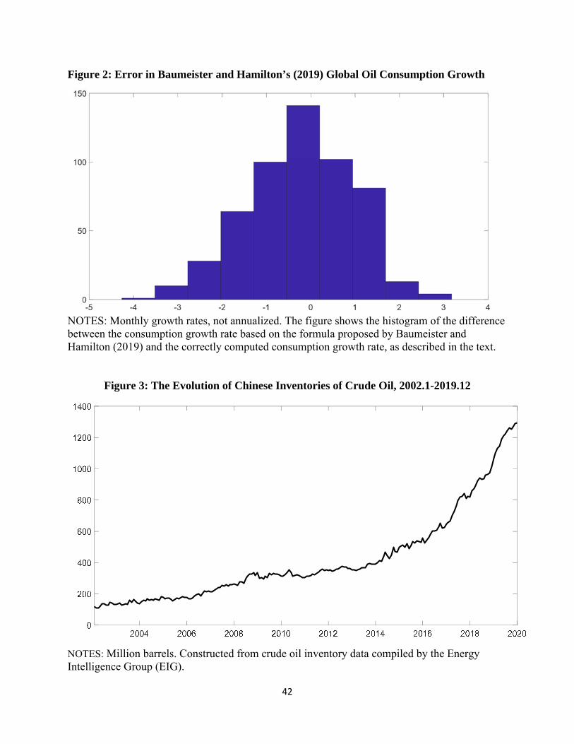
42  

Figure 2: Error in Baumeister and Hamilton’s (2019) Global Oil Consumption Growth

NOTES: Monthly growth rates, not annualized. The figure shows the histogram of the difference between the consumption growth rate based on the formula proposed by Baumeister and Hamilton (2019) and the correctly computed consumption growth rate, as described in the text.

Figure 3: The Evolution of Chinese Inventories of Crude Oil, 2002.1-2019.12

NOTES: Million barrels. Constructed from crude oil inventory data compiled by the Energy Intelligence Group (EIG).

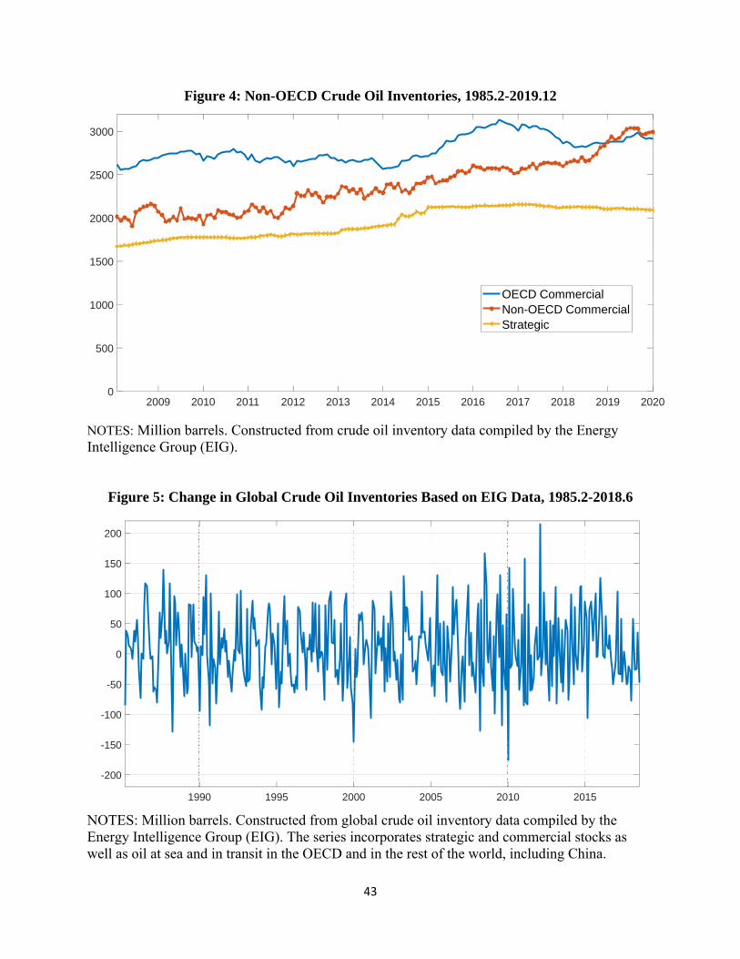
43  

1990 1995 2000 2005 2010 2015

-200

-150

-100

-50

0

50

100

150

200

2009 2010 2011 2012 2013 2014 2015 2016 2017 2018 2019 20200

500

1000

1500

2000

2500

3000

OECD CommercialNon-OECD CommercialStrategic

Figure 4: Non-OECD Crude Oil Inventories, 1985.2-2019.12 NOTES: Million barrels. Constructed from crude oil inventory data compiled by the Energy Intelligence Group (EIG).

Figure 5: Change in Global Crude Oil Inventories Based on EIG Data, 1985.2-2018.6

NOTES: Million barrels. Constructed from global crude oil inventory data compiled by the Energy Intelligence Group (EIG). The series incorporates strategic and commercial stocks as well as oil at sea and in transit in the OECD and in the rest of the world, including China.

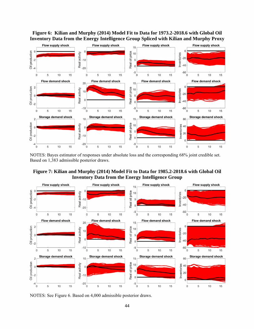
44  

Figure 6: Kilian and Murphy (2014) Model Fit to Data for 1973.2-2018.6 with Global Oil Inventory Data from the Energy Intelligence Group Spliced with Kilian and Murphy Proxy

NOTES: Bayes estimator of responses under absolute loss and the corresponding 68% joint credible set. Based on 1,383 admissible posterior draws.

Figure 7: Kilian and Murphy (2014) Model Fit to Data for 1985.2-2018.6 with Global Oil Inventory Data from the Energy Intelligence Group

NOTES: See Figure 6. Based on 4,000 admissible posterior draws.