faculdade de engenharia da universidade do porto · arma autoregressive mean average bp back...
TRANSCRIPT

Faculdade de Engenharia da Universidade do Porto
SHORT-TERM FORECASTING OF PHOTOVOLTAIC POWER
PLANTS
Pedro Henrique Cardeal Serra
Thesis written in the ambit of Master in Electrical and Computers Engineering Major in Energy
Advisor: José Nuno Fidalgo (Dr.)
Co-Advisor: Ricardo Bessa (Dr.)
January 2014

ii

© Pedro Henrique Cardeal Serra, 2014

iv

Abstract
Solar power is the biggest source of energy that humanity has access to. Although the solar
energy is not the most used source of renewable energy its share in the global power
production has been increasing. Solar power forecasting is a key tool for the integration of
this kind of energy production into the grid, enabling an efficient management and control of
the power generation system. Thus, the aim of the present thesis is the development of a
solar power forecasting method.
There are several Numerical Weather Predictions (NWP) variables which can influence the
solar power production of a PV panel, and were tested in this work; this includes variables
such as Global Horizontal Irradiance, Direct Normal Irradiance, and Cloudiness, among others.
This thesis presents a short-term forecasting method for photovoltaic power production, in
this specific case a forecast is made for a time span of 72 hours ahead. This forecasting
method is based on Extreme Learning Machines, a relatively new statistical method. The
present method uses a combination of NWP and series of past values, thus being classified as
a hybrid method.
The forecast for the time span is made for each hour separately and has the capacity to start
at whatever hour is suited for the electricity market or the power producer.
The performance of the forecasting method is rated by an error measure process, the results
were better for the first 5 hours of the time span beginning below 6% for the first hour and
steadily rising to around 9%, once they use series of the past power production values as
input, for the span of the hours 6-72 the Numerical Weather Predictions were found to be a
more relevant input with an error always rounding 11%.
Keywords: Solar Power, Extreme Learning Machines, Photovoltaic Forecasting, Numerical
Weather Predictions, Irradiance, Renewable Energies.

vi

Resumo
A energia solar é a maior fonte de energia a que a humanidade tem acesso. Apesar de a
energia solar não ser a fonte de energia renovável mais utilizada a sua quota-parte na
produção global de energia tem vindo a subir. A previsão fotovoltaica é um instrumento chave
para a integração da produção das energias renováveis na rede, fazendo com que seja
possível uma gestão e controlo mais eficiente do sistema electroprodutor. Assim, o principal
foco da presente dissertação é o desenvolvimento de um modelo de previsão fotovoltaica.
Existem várias variáveis Numerical Weather Predictions (NWP) que podem influenciar a
produção de um painel fotovoltaico e que foram testadas no presente trabalho; isto inclui
variáveis tais como irradiância global horizontal, irradiância direta e nebulosidade, entre
outras.
Esta tese apresenta um método de previsão da produção fotovoltaica a curto-prazo, mais
especificamente, uma previsão é feita para um período de 72 horas à frente. Este método de
previsão é baseado em Extreme Learning Machines, um método estatístico relativamente
recente. O presente método combina NWP e séries de valores passados, sendo assim
classificado como um método hibrido.
A previsão é feita em separado para cada uma das horas do espaço temporal e tem também a
capacidade de começar a qualquer hora do dia, de maneira a ser mais conveniente para o
mercado ou para o produtor.
A performance do método de previsão desenvolvido é avaliado com um procedimento de
medido do erro, os resultados foram melhoras para as primeiras 5 horas do horizonte de
previsão, começando abaixo dos 6% para a primeira hora do horizonte subindo até por volta
dos 9% para a quinta hora, uma vez que estas usam valores passados para a sua previsão, para
o horizonte das 6-72 horas as NWP revelaram-se variáveis de entrada de maior importância do
que para as primeiras horas tendo assim um erro associado que ronda os 11%.
Palavras-chave: Energia Solar, Extreme Learning Machines, Previsão Fotovoltaica, Numerical
Weather Predictions, Irradiância, Energias renováveis.

viii

Acknowledgements
This moment offers the opportunity to thank to every person and institution which, directly or
indirectly, helped and contributed to the elaboration of the present thesis.
Firstly, to my advisors Dr. José Nuno Fidalgo and Dr. Ricardo Bessa, for all their help and
experience which proved to be of great value in the course of the present work. Also, for the
availability demonstrated in the long hours of reunions and discussions throughout the
semester. Without their guidance this thesis would not have been possible.
To the opportunity to do this thesis, a note of thanking is due to INESC Porto (Instituto de
Engenharia de Sistemas e Computadores do Porto).
To all my colleagues and friends who accompanied me during this stage of my life, for the
support, friendship and companionship demonstrated during not only the long hours of study
and work, but also outside college.
To my family who provided the best conditions for my education and academic path as well as
my personal and professional realization.
Lastly, but not at all less important, to my girlfriend Maria, who supported me in every
moment of this last journey as a student and whose constant presence and encouragement
always kept me focused.
This work was developed in the framework of the BEST CASE project (“NORTE-07-0124-FEDER-
000056”) financed by the North Portugal Regional Operational Programme (ON.2 – O Novo
Norte), under the National Strategic Reference Framework (NSRF), through the European
Regional Development Fund (ERDF), and by national funds, through Fundação para a Ciência e
a Tecnologia (FCT). It was also developed within FCT projects «SMAGIS – PTDC/SEN-
ENR/113094/2009» and «DYMONDS – CMU-PT/SIA/0043/2009».

x

“Chaos is the score upon which reality is written.”
-Henry Miller

xii

Contents
Abstract ............................................................................................. v
Resumo ............................................................................................ vii
Acknowledgements .............................................................................. ix
Contents .......................................................................................... xiii
Figure List ........................................................................................ xvi
Table List ....................................................................................... xviii
Abbreviations and Symbols ................................................................... xix
Chapter 1 ............................................................................................. 1
Introduction ....................................................................................................... 1
1.1. Motivation ............................................................................................... 2
1.2. Relevance of Forecasts ............................................................................... 6
1.3. Objectives ............................................................................................... 7
1.4. Structure ................................................................................................ 8
Chapter 2 ............................................................................................. 9
Background ........................................................................................................ 9
2.1. Photovoltaic Systems .................................................................................. 9
2.2. Numerical Weather Predictions ................................................................... 13
2.2.1. GHI – Global Horizontal Irradiance ........................................................... 13
2.2.2. DNI – Direct Normal Irradiance ............................................................... 15
2.2.3. Temperature ..................................................................................... 15
2.2.4. Cloudiness ........................................................................................ 15
2.2.5. Solar Altitude .................................................................................... 16
Chapter 3 ............................................................................................ 18
State of the Art ................................................................................................ 18
3.1. Solar Forecasting Models ........................................................................... 18
3.1.1. Physical Models .................................................................................. 19
3.1.2. Computational Models ......................................................................... 23
3.2. Final Remarks ......................................................................................... 27
Chapter 4 ............................................................................................ 28
Methodology .................................................................................................... 28

xiv
4.1. Artificial Neural Networks .......................................................................... 28
4.2. Support Vector Machines ........................................................................... 31
4.3. Extreme Learning Machines ........................................................................ 31
4.3.1. ELM Basics ........................................................................................ 31
4.3.2. ELM vs. Neural Networks ...................................................................... 34
4.3.3. ELM vs. SVMs ..................................................................................... 34
4.4. Data Treatment ...................................................................................... 35
4.4.1. Data Organization and Synchronization ..................................................... 35
4.4.2. Clear Sky Model ................................................................................. 36
4.4.3. Standardization ................................................................................. 37
4.4.4. Training and Testing Sets ..................................................................... 37
4.5. Forecasting Model Layout .......................................................................... 38
4.6. Activation Functions ................................................................................ 41
Chapter 5 ............................................................................................ 44
Results and Discussion ........................................................................................ 44
5.1. Data used .............................................................................................. 44
5.2. NWP Analysis ......................................................................................... 45
5.3. Error Measures ....................................................................................... 51
5.4. Forecasting Model Evaluation ..................................................................... 52
5.4.1. Choosing the NWP forecasting set ........................................................... 52
5.4.2. Choosing the Activation Function ............................................................ 54
5.4.3. Forecasting Results ............................................................................. 55
5.5. Forecasting Model performance ................................................................... 59
5.6. Comparison with other Methods .................................................................. 60
Chapter 6 ............................................................................................ 64
Conclusion....................................................................................................... 64
6.1. Future Works ......................................................................................... 65
Bibliography .................................................................................................... 67
Appendixes ........................................................................................ 72
Appendix A ......................................................................................... 72
Clear Sky Model ................................................................................... 72
Appendix B ......................................................................................... 75
Moore-Penrose generalized inverse matrix ................................................... 75


xvi
Figure List
Figure 1.1 - Proportions between traditional energy sources and renewable energy sources [4] .......................................................................................................... 2
Figure 1.2 - Global investments in renewable energy [7] .............................................. 3
Figure 1.3 - Investment by technology 2004-2011 [80] ................................................. 4
Figure 1.4 - Global mean solar irradiance [10] ........................................................... 5
Figure 1.5 - Projections for annual solar PV capacity and revenue [9] .............................. 6
Figure 2.1 - Major PV system components [14] ......................................................... 10
Figure 2.2 - Schematics of PV array components [13] ................................................ 11
Figure 2.3 - Angle representation following solar techniques [16] ................................. 12
Figure 2.4 - Winter and Summer panel inclinations[17] .............................................. 13
Figure 2.5 – Irradiation of a Horizontal Surface [46] .................................................. 14
Figure 2.6 – Zenith angle [51] ............................................................................. 17
Figure 3.1 - Motion vector fields calculated in short-term forecasting scheme [21] ............ 20
Figure 3.2 – An example of the planet divided into a 3-D grid for the purpose of NWP [30] ... 21
Figure 3.3 - a) Dow Jones index on 292 consecutive days; b) Daily change in Dow Jones 292 consecutive days [18] ........................................................................... 24
Figure 4.1 - Schematization of an artificial neural networks's neuron model [27] ............... 29
Figure 4.2 - Example of an artificial neural network with layers ................................... 30
Figure 4.3 - Structure of an ELM network ............................................................... 32
Figure 4.4 – Diagram representing the forecasting model overview ................................ 38
Figure 4.5 - Diagram representing the training and testing structure ............................. 39
Figure 4.6 - Simplified scheme of the forecasting model for every hour oh the time span .... 41
Figure 5.1 - Scatter graphic of Power vs. forecasted DNI ........................................... 45
Figure 5.2 - Scatter graphic of Power vs. measured DNI ............................................. 46
Figure 5.3 - Scatter graphic of Power vs. forecasted GHI ............................................ 47

Figure 5.4 - Scatter graphic of Power vs. measured GHI ............................................. 47
Figure 5.5 - Scatter graphic of Power vs. forecasted Cloudiness ................................... 48
Figure 5.6 - Scatter graphic of Power vs. forecasted Temperature 2 meters above ground ... 48
Figure 5.7 - Scatter graphic of Power vs. measured Temperature 2 meters above ground .... 49
Figure 5.8 - Scatter graphic of Power vs. forecasted Solar Altitude................................ 49
Figure 5.9 - Scatter graphic of Power vs. measured Solar Altitude ................................. 50
Figure 5.10 - Forecast made for April's 29th at 00:00 UTC for the next 3 days................... 55
Figure 5.11 - Forecasting error for the span of April's 29th to May's 1st ............................ 56
Figure 5.12 - Forecast made for August’s 20th at 00:00 UTC for the next 3 days................ 56
Figure 5.13 - Forecast made for April's 3rd at 9:00 UTC for the next three days ................. 57
Figure 5.14 - Forecasting error for the span of April's 3rd to April's 5th ........................... 57
Figure 5.15 - Forecast made for December’s 4th at 9:00 UTC for the next three days .......... 58
Figure 5.16 - Forecasting error for the span of December's 4th to December's 6th ............. 58
Figure 5.17 - NMAE vs. Forecasting Horizon for the Hybrid ELM model ............................ 59
Figure 5.18 - NMAE vs. Forecasting Horizon for Autoregressive ELM model ....................... 59
Figure 5.19 - NMAE vs. Forecasting Horizon for the NWP ELM model .............................. 60
Figure 5.20 - NMAE vs. Forecasting Horizon for the ANN model ..................................... 62
Figure 5.21 - NMAE vs. Forecasting Horizon for the SVM model ..................................... 62

xviii
Table List
Table 1 – GHI, DNI and Temperature 2 meters above ground forecasting errors ................. 50
Table 2 - NMAE for the test set for several combinations of NWP and the respective neurons which provided the best forecast for each case ...................................... 53
Table 3 - Activation Function with corresponding NMAE (%) ......................................... 54
Table 4 - Activation Functions with corresponding Training and Testing Times (in seconds) and Neurons used to achieve the best results ................................................... 54
Table 5 - NMAE (in percentage) for the referred statistical models ................................ 61
Table 6 - Training and Testing times of the statistical methods (in seconds) .................... 61

Abbreviations and Symbols
Abreviation List
ANN Artificial Neural Network
AR Autoregression
ARIMA Autoregressive integrated mean average
ARMA Autoregressive mean average
BP Back Propagation
DEEC Departamento de Engenharia Eletrotécnica e de Computadores
DHI Diffuse Horizontal Irradiance
DNI Direct Normal Irradiance
ECMWF European Centre for Medium-Range Weather Forecasts
ELM Extreme Learning Machines
FEUP Faculdade de Engenharia da Universidade do Porto
GHI Global Horizontal Irradiance
GTS Global Telecommunication System
LS Least Square
LS-SVM Least Square Support Vector Machine
MAE Mean Average Error
MLP Multilayer Perceptron
MSG Meteosat Second Generation
NDFD National Digital Forecast Database
NN Neural Network

xx
NWP Numerical Weather Predictions
PSVM Proximal Support Vector Machine
PV Photovoltaic
PWL Piece-Wise Linear
RAMS Regional Atmospheric Modeling System
RBF Radial Basic Function
RBF Radial Basis Function
RMSD Root Mean Square Deviation
RMSE Root Mean Square Error
SLFN Single-layer Feedforward Network
SVD Single Value Decomposition
SVM Support Vector Machines
SVR Support Vector Regression
TBF Triangular Basis Function
TDNN Time Delay Neural Network
VC Vapnik-Chervonenkis
WMO World Meteorological Organization
Symbol List
Elevation angle
Declination angle
Latitude of the current location
Solar azimuth
Solar elevation angle
α Collector azimuth
β Collector elevation angle
Differenced series
Vector of the output weights between the hidden layer and the output node

Output vector of the hidden layer
H Hidden layer output matrix
Moore-Penrose generalized inverse matrix
Produced power one hour before the forecasting
Produced power one day before the hour for which the forecast is made
K Hour which will be forecasted
D Day for which the forecast will be made
Solar Power
Clear sky solar power
Normalized solar power
Measured power production
Forecasted power production
G Global Irradiance
Clear sky global irradiance
Transmissivity of the clouds
Extraterrestrial irradiance
Total sky transmissivity in clear sky
p Solar power
Clear sky power
Clear sky estimated solar power


Chapter 1
Introduction
This thesis was developed in the ambit of the Master in Electrical and Computers Engineering
at Faculdade de Engenharia da Universidade do Porto (FEUP).
The renewable energies are increasingly earning its share in the energetic outlook, even
getting at times bigger stakes than traditional energy sources, such as fossil and nuclear, e.g.
in Portugal during 2013 there were some days of 100% renewable energy output [6]. With its
increasingly demand for energy, humanity needs to invest in this type of power sources and
solar power is potentially the biggest one we have access to, as can be seen in Figure 1.1.
In the present thesis a forecasting method for photovoltaic micro-generation is developed
using forecasting up to 72 hours ahead using Extreme Learning Machines (ELM) which allows
non-linear relationships between power production and numerical weather predictions
(NWP). The data used is from a real source located in southern Italy, having, therefore,
similar latitude to Portugal.

2 Introduction
2
1.1. Motivation
Throughout history, especially since the industrial revolution the energetic demand of
populations has been exponentially increasing, making the meeting of those demands a huge
problem that governments are facing. The eminence of fossil energy sources depletion as well
as the United Nations’ pressures concerning greenhouse gases emissions through the Kyoto
protocol, have been forcing a turn of investments into renewable energy sources such as
photovoltaic and aeolian. The investments in this energy sources have been increasing for the
great length of the last decade with a little decrease in 2012, as can be seen in Figure 1.2
and Figure 1.3, the appointed reason being due to the difficult global financial environment
that has affected many sectors and many investors are not in a disposition to risk much funds
also due to the governments energy policy reforms [8]. Also, the prices of the solar modules
have been falling with the evolution of the technology, which can explain, in addition, the
fall of the investments.
Figure 1.1 - Proportions between traditional energy sources and renewable energy sources [4]

3 Motivation
The focus of the present thesis resides in solar power forecasting which has an
insurmountable capability as seen above in Figure 1.1. Especially in countries like Portugal
and Italy which have an annual irradiance considerably high (Figure 1.4), that should be an
encouragement for increasing investments. In the latest years the governments have been
funding renewable energy production aiming to achieve Kyoto’s protocol commitments as
well as reducing their dependency from fossil energy sources.
Figure 1.2 - Global investments in renewable energy [7]
4 Introduction
4
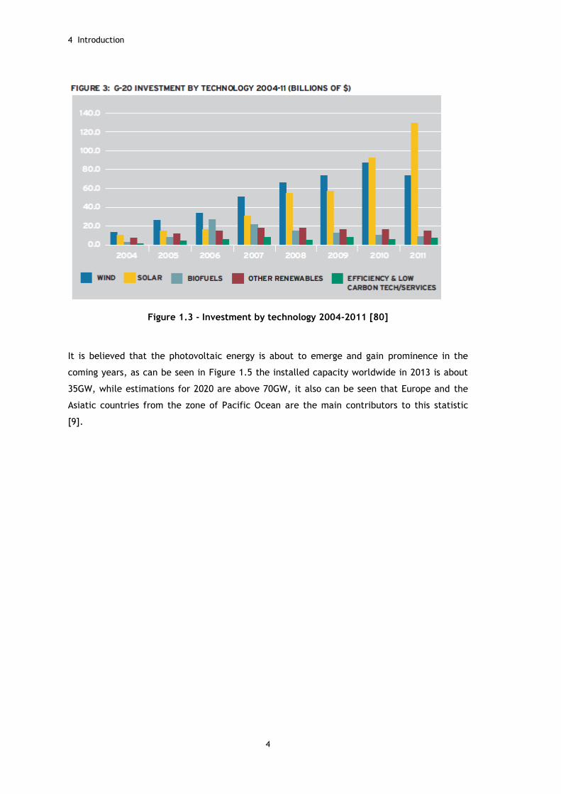
Figure 1.3 - Investment by technology 2004-2011 [80]
It is believed that the photovoltaic energy is about to emerge and gain prominence in the
coming years, as can be seen in Figure 1.5 the installed capacity worldwide in 2013 is about
35GW, while estimations for 2020 are above 70GW, it also can be seen that Europe and the
Asiatic countries from the zone of Pacific Ocean are the main contributors to this statistic
[9].

5 Motivation
Aside from ecological problems governments have been facing, another issue is the fairness
between the incentives given to renewable energy producers and competitive prices. These
incentives are necessary in order to galvanize and help the development of this kind of power
producers.
Also, some countries have managed to create an energy market system, some markets even
comprise several nations e.g. the MIBEL including Portugal and Spain, the forecasts are
extremely important for the markets as a tool, as will be seen later in the following section.
The MIBEL is the platform where all electricity concerning Iberia is transacted setting the
prices for every hour of the following day. The daily market session is made at 11 a.m.
Portuguese time. The hourly market prices are established by crossing both the selling and
buying offers by every agent able to operate in that market. Each offer must point the day
and hour for which it is making an offer, as well as the corresponding price and power. The
price is found by a process wherein the selling offers are organized in crescent order by price
while the buying offers are organized in descent order by price for each hour of the day, and
then the market price is given by the point where both curves graphically cross each other.
This means the price is the same for every agent who takes part in the auction [5].
Figure 1.4 - Global mean solar irradiance [10]

6 Introduction
6
Figure 1.5 - Projections for annual solar PV capacity and revenue [9]
1.2. Relevance of Forecasts
The relevance of renewable energies has been rising substantially in the last two decades,
and this growth is expected to persist in the current in the next years, headed by Aeolian and
Photovoltaic energies. The volatility of this kind of energy brings out a new problem: If the
energy sources cannot be tamed, how can its output be controlled so it can be safely used?
The answer to this question has been partly given by the power production forecasts, which
can help to greatly diminish a number of issues:
Great variability in weather sources, e.g., wind and sun;
The need for a great service quality by the grid and power production;
The more renewable energy sources the more vulnerable is the system;
Power markets demand the anticipation of production quantities of each producer;
The need for system reserves planning;
Planning interconnections between different grids [2], [12].
Because of the aforementioned reasons it is extremely important that the technologies used
in forecasting, keep developing and increasing its performance because they are fundamental
to the efficiency of the system and thus, to mankind as well.
Energy efficiency and conservation are important measures that should be considered in
conjunction with PV systems. These systems provide a buffer against rising energy prices, and

7 Objectives
the presence of an on-site battery bank can supply electricity during utility power outages.
Solar power can also help make a difference in the way that we address climate change and
the impact on the environment.
There are several ranges of forecasting:
Long-term forecasting, which is used for an horizon of 5 years up to 25, it is
important for grid expansion planning, creating good conditions for short-term
expansions;
Mid-Term forecasting, which is used for an horizon of a few months up to a few years,
it is important for financial and expansion planning and maintenance programming;
Short-term forecasting is used for a horizon of a few hours up to few weeks and it is
used for the operation of the grid in short-term [11].
Another important parameter of forecasts is the spatial load forecasting, i.e., the service
area of the power producer. The forecasts in this case are important for financial planning,
and are often based on macroeconomic aspects, commercial info and time series. This type
of forecasting is usually simple because of the great availability of information, internal and
external [11];
There are several forecasting models and techniques which range from regression models
passing by stochastic models of time series to computational intelligence, which includes
artificial neural networks (ANN) that are the foundation for this dissertation. The neural type
of ANN used in this work is known by ELM (Extremely learning machines) and it will be
presented later on in this document. The forecasting models used in the present work use
NWP (Numerical Weather Predictions) as a ground base, and it can include, e.g., Irradiation,
Temperature, Solar altitude, Wind speed [11].
1.3. Objectives
The intention of the present thesis is to create a model for short-term forecasting (i.e. up to
72 hours ahead), using auto-learning techniques, of Photovoltaic power plants. The main
objective consists in applying innovative concepts based on Extreme Learning Machines (ELM)
with variable coefficients, allowing the modelization of non-linear relations between the
power plant production and Numerical Weather Predictions (NWP).
The experimentation with several different activation functions is also an integrant part of
this thesis in order to understand its effects on the results and to discover which activation
function provides better results.

8 Introduction
8
1.4. Structure
The present thesis is constituted by six chapters, being the present chapter dedicated to the
introduction of the proposed problem.
The second chapter presents a review of the background of PV systems. It starts by a short
introduction about photovoltaic power systems and its constituents. Follows a presentation of
the most common weather variables used In PV power output forecasting, such as Global
Horizontal Irradiance or Direct Normal Irradiance.
The third chapter is dedicated to the presentation of the State of the Art, and does an
overview of various forecasting models which are commonly used for PV power output
forecasting. In the end of the chapter some final remarks about the study are made.
The fourth chapter describes the methodology used in this work. This includes the
presentation in some degree of detail of the ELM technique, which is a main factor for the
development of the work that led to the elaboration of the present document as well as
other statistical methods. Also, it is made a comparison between the ELM and these other
statistical methods. The data treatments techniques utilized in the development of this work
are also presented in this chapter as well as the forecasting model layout.
The fifth chapter presents the discussion and results of this work. A deep insight over the
used Numerical Weather Predictions is also given. In addition, an overview of the error
measures used in the course of the method is given. Finally, the results are presented and
discussed.
The sixth chapter presents the conclusions drawn with this work. A critical analysis is also
made. Lastly, some options of future work are presented.

Chapter 2
Background
This chapter presents some aspects of photovoltaic systems. Also, some of the typical
photovoltaic power forecasting methods are presented. An insight over the most influential
Numerical Weather Predictions for PV forecasting is provided as well.
2.1. Photovoltaic Systems
Photovoltaic (PV) systems are used to convert sunlight to electricity. They are a safe,
reliable, low-maintenance source of solar electricity that produces no on-site pollution or
emissions. PV systems incur few operating costs and are easy to install on most houses. These
systems fall into two main categories – off-grid and grid-connected. The “grid” refers to the
local electric utility’s infrastructure that supplies electricity to houses and businesses. Off-
grid systems are installed in remote locations where there is no utility grid available.
Internationally, utility grid-connected PV systems represent the majority of installations,
growing at a rate of 20-30% annually. However, the number of grid-connected systems
continues to grow because many of the barriers to interconnection have been addressed
through the adoption of harmonized standards and codes. In addition, policies supporting grid
interconnection of PV power have encouraged a number of building-integrated PV
applications [13].
With the rising of electricity costs, concerns to the reliability of the continuous service
delivery and increased environmental awareness of homeowners, the demand for residential
PV systems is increasing [13].

10 Background
10
Simply put, PV systems are like any other electrical power generating systems. However, the
principles of operation and interfacing with other electrical systems remain the same, and
are guided by a well-established body of electrical codes and standards.
Although a PV array produces power when exposed to sunlight, a number of other
components are required to properly conduct, control, convert, distribute, and store the
energy produced by the array.
Depending on the functional and operational requirements of the system, the specific
components required may include major components such as DC-AC power inverter, battery
bank, system and battery controller, auxiliary energy sources and sometimes the specified
electrical load. In addition, an assortment of balance of system hardware, including wiring,
over current, surge protection and disconnect devices, and other power processing
equipment. Figure 2.1 shows a basic diagram of a PV system and the relationship of individual
components [14].
Batteries are often used in PV systems for the purpose of storing energy produced by the PV
array during the day, and to supply it to electrical loads as needed. This happens most often
when it’s a non grid-connected PV system, although grid-connected systems may include a
battery bank.
The most critical component of any PV system is the PV module, which is composed of a
number of interconnected solar cells. PV modules are connected together into panels and
arrays to meet various energy needs, as shown in Figure 2.2 [13].
Figure 2.1 - Major PV system components [14]

11 Photovoltaic Systems
There are several factors that can influence the output (energy production) of a PV system,
although the most important factors are the irradiation and cell temperature. The current
produced in modules is linearly linked to the light intensity, thus when irradiance rises the
produced electricity will rise as well. Another important factor is the cell temperature, i.e.,
the rise of cell temperature decreases the efficiency of the module, preventing it to function
at maximum power [15]. Another factor to be considered in the phase of panel installation is
the wind speed which is important, for accounting the mechanical forces that the array is
subjected to.
The knowledge of the exact location of the sun is indispensable for determining the radiation
data and the power produced by solar installations. The location of the sun can be defined
anywhere by its height and azimuth. In solar energy fields the South is usually referred as
α=0º. The negative values are attributed to the East angles (α=-90º) and the positives are
attributed to West angles (α=90º).
Figure 2.2 - Schematics of PV array components [13]

12 Background
12
is the solar azimuth, is the solar elevation angle, α is the collector azimuth and β is the
collector elevation angle [16].
The quantity of solar radiation captured by a surface is maximized when the panel surface is
perpendicular to the radiation. This fact is related to the angular absorption variation and to
the reflection, as well as to the path followed by the radiation. The inclination of the PV
array should optimize the capture of the solar radiation, accounting on elevation and solar
azimuth throughout the year, as can be seen in Figure 2.4.
Figure 2.3 - Angle representation following solar techniques [16]

13 Numerical Weather Predictions
2.2. Numerical Weather Predictions
A wide variety of weather phenomena can be analyzed and predicted by several different
types of numerical weather prediction models. The numerical weather predictions used for
certain kinds of forecasting differ from case to case, e.g., for photovoltaic systems
forecasting, the wind speed is not a variable as relevant as global horizontal irradiance, as
opposed to wind power forecasting, which takes it as its most important variable. Also, there
is a number of variables that may or may not be of importance for some kinds of forecasting
models, and they have to be tested so a decision on its inclusion on the forecasting method or
not may be responsibly taken.
In this section the available numerical weather predictions for this case are explained, and
then discussed for a conclusion on its addition to the model or not is reached.
2.2.1. GHI – Global Horizontal Irradiance
The total solar radiation reaching the surface of the earth can be represented in several
different ways. Global Horizontal Irradiance (GHI) is the quantity of short wave irradiance
falling on the surface of the earth or a surface horizontal to the ground. The GHI is
particularly interesting to photovoltaic installations and is composed by both Direct Normal
Figure 2.4 - Winter and Summer panel inclinations[17]

14 Background
14
Irradiance (DNI) and Diffuse Horizontal irradiance (DHI). DNI is solar radiation directly applied
to earth coming in a straight line from the position of the sun in the sky. DHI is solar radiation
which has been scattered by molecules and particles in the atmosphere and comes in the
same amount from all directions. On a cloudy day, most of the solar irradiance received by
the earth’s surface comes from DHI, while on a clear day, it will mostly come from DNI [44]
[45].
The most common instrument to measure GHI is a pyranometer which has a viewing angle of
180º (hemispherical). The trademark of the pyranometer is a true cosine response to incident
angle, i.e. its response to a solar beam is proportional to the cosine of the incident angle of
the beam. Most pyranometers utilize a thermopile sensor to sense the incoming beams of
light. GHI may also be measured with a photovoltaic reference cell, which has a spectral
sensitivity and generally will not reveal true cosine response.
If the GHI cannot be directly measured, it may be calculated from DNI and DHI using the
subsequent equation [45]:
In Figure 2.5 both the factors by which the Global Horizontal Irradiance is composed can be
seen:
Figure 2.5 – Irradiation of a Horizontal Surface [46]

15 Numerical Weather Predictions
2.2.2. DNI – Direct Normal Irradiance
Direct Solar Irradiance, also known as Direct Normal Irradiance (DNI) is a measure of the rate
of solar energy arriving at the Earth’s surface directly from the Sun’s direct light beam, on a
plane perpendicular to the beam, and usually is measured by a pyrheliometer mounted on a
solar tracker. This tracker guarantees that the sun beam is always directed into the
pyrheliometer field of view, during the day time. The pyrheliometer has a field of view of 5º.
In order to use this measure for comparison with global and diffuse irradiances, it is required
to obtain the horizontal element of the direct solar irradiance. This is obtained by multiplying
the direct solar irradiance by the cosine of the Sun’s zenith angle [47].
To maximize the quantity of irradiance received by a surface it is needed to keep it normal to
the incoming radiation. This quantity is of particular interest to concentrating solar thermal
installations and installations that track the position of the sun [48].
Figure 2.5 illustrates these concepts.
2.2.3. Temperature
Temperature can be defined as the measure of hotness or coldness of an object or of the
environment that can be measure by using a thermometer [71]. In what concerns forecasting,
temperature usually uses Kelvin as a unit, but it can also be measure in Celsius or in
Fahrenheit.
Temperature is mostly important for photovoltaic forecasting because of the functioning of
the panels, i.e., if the temperature is too high, the photovoltaic panels will start
malfunctioning, which lowers their efficiency and consequently is bad for power production.
When the opposite occurs, in certain cases, the panels can show a better performance due to
the low temperature provided by the environment. So, although it is not a factor as relevant
as Global Horizontal Irradiance or Direct Normal Irradiance for the forecasting, temperature
can, in certain occasions, be important.
2.2.4. Cloudiness

16 Background
16
Seen from space, Earth is a blue planet strongly marked by white cloud structures. By
reflecting sunlight, blocking outgoing longwave radiation and producing precipitation, clouds
are a factor of great impact in the Earth’s climate. The single major source of uncertainty in
global climate models has only been of the clouds responsibility, especially when they are
running low. Nowadays it is still a challenge to model the clouds conduct. Therefore, it is of
great relevance to monitor changes in Earth’s cloud cover and movements [49].
Habitually, the clouds behavior has been observed at naked eye by trained technicians at
weather stations or at onboard ships around the world, following the rules of the World
Meteorological Organization (WMO). Then, the collected data is transmitted through the
Global Telecommunication System (GTS) in real time to weather stations all around the world
[49].
In what concerns the solar forecasting, one of the most important factors of photovoltaic
systems is the predictability of solar radiation, which is greatly dependent on cloudiness,
which occurrence is a non-linear process [50]. This doesn’t mean that when a cloudy day
happens, the PV system stops functioning, it stills produces power, although not in the
quantity it would in a clear sky day. This is called low-light condition performance.
2.2.5. Solar Altitude
Solar altitude refers to the angular height of the sun in the sky measured from the horizon.
The elevation is 0º at sunrise and 90º when the sun is directly overhead, which may never
truly happen, depending on the location’s latitude. The elevation angle varies during the day,
and is also dependent of the latitude of the location and of the time of the year. An
important parameter in the design of photovoltaic systems is the maximum elevation angle,
that is, the maximum height of the sun in the sky at a particular time of year. This is
important for photovoltaic systems, because it can affect the intensity of the energy that
reaches solar panels [51].
While the maximum elevation angle is used even in very simple PV systems design, more
precise PV systems require the exact variation of the maximum angle throughout the day.
The elevation angle can be calculated using the following equation:
Where,
is the elevation angle;
is the declination angle;
is the latitude of the current location;

17 Numerical Weather Predictions
HRA is the hour angle.
The zenith angle is the angle between the sun and the vertical. The zenith angle is similar to
the elevation angle but it is measured from the vertical rather than the horizontal, thus
making the zenith angle ( ) = 90º - elevation [51]. This can be seen next in Figure 2.6.
Figure 2.6 – Zenith angle [51]

Chapter 3
State of the Art
The power output of a photovoltaic system is very dependent of the weather conditions,
especially the global horizontal irradiance. As the irradiance is very unstable, varying not only
seasonally but also daily, it comes out as a challenging forecasting object. The importance of
photovoltaic power output forecasting is therefore of great relevance. This chapter presents
a review over some photovoltaic power forecasting models and does a review over the state
of the art of such models.
With the study of the state of the art will be possible to better understand the relevance of
the present thesis and its innovations.
3.1. Solar Forecasting Models
Solar radiation is the driving force behind a number of solar energy devices with a great range
of action and operating principles such as the aforementioned photovoltaic systems which
generate energy, solar collectors for building heating, air conditioning climate control in
buildings and some passive solar devices such as windows, walls or even floors [19].
As stated before, the introduction of renewable energy in the markets has been gradually
rising, but it still is a big controversy source. It has undoubtedly a great potential in terms of
economic and environmental causes, but its instability and great volatility, are the big
challenge to be surpassed.
Along the years some methods targeting the solution to this problem have been developed.
The forecasting horizon is a very import factor, since some methods are better for a
particular horizon than others. Therefore, this chapter describes some of these methods.

19 Solar Forecasting Models
Also, a necessary remark concerning this state of the art section is the difficulty in finding
previous work in the particularity of this thesis which is hybrid models between
Autoregressive and Numerical Weather Prediction models. Photovoltaic power production is
notoriously rising throughout the world and when the PV forecasting existing studies is
compared to the corresponding offer for wind farm power production forecasting it stands
out the gap between both technologies, with prejudice to the PV power production
forecasting.
3.1.1. Physical Models
3.1.1.1. Solar irradiance forecast using satellite images
As far as short-term horizons are concerned, satellite data are a high quality source for
radiance information because of its excellent temporal and spatial resolution. Due to the
strong impact of cloudiness on surface solar irradiance, an accurate description of the
temporal development of the cloud situation is essential for irradiance forecasting. As a
measure of cloudiness, cloud index images according to the Heliosat method [35], a semi-
empirical method to derive solar irradiance from satellite data, are calculated from the
satellite data. To predict the cloud index image in a first step motion vector fields are
derived from two consecutive images. The future image then is determined by applying the
calculated motion vector field to the actual image. At last, solar surface irradiance is derived
from the predicted cloud index images with the aid of the Heliosat method [21].
As a measure of cloudiness a dimensionless cloud index value n for each image pixel is
derived. A basically linear relationship is assumed to describe the influence of the cloud
index on the atmospheric transmittance. The global irradiance is calculated by combining the
information on the atmospheric transmission with a clear sky model.
Typical deviations of hourly satellite-derived global irradiance from ground truth data are 20-
25% of relative root mean square error (RMSE) for Meteosat7. For the new satellite generation
Meteosat second generation (MSG) and using further enhanced irradiance calculation schemes
these errors are reduced with a factor of approx. 0.9. The quality of the satellite-derived
irradiance provides a lower limit for the forecast accuracy [23].

20 State of the Art
20
Figure 3.1 - Motion vector fields calculated in short-term forecasting scheme [21]
3.1.1.2. Numerical Weather predictions
Very short-term forecasting of global solar irradiance with a limited time horizon of
approximately 6h is not sufficient for an efficient planning and operation of solar energy
systems. Especially for the grid integration of solar energy forecasts for up to 48h or even
beyond have to be provided. Numerical meteorological models may have the potential to
satisfy the requirements in forecasting solar irradiance. A meteorological model is any model
which allows calculating fields of meteorological variables, e.g., wind speed, radiation in the
atmosphere. Global NWP models have usually a coarse resolution and do not allow for a
detailed mapping of small-scale features. Therefore, the use of regional mesoscale models
and the combination of a NWP model with a statistical post-processing tools to account for
local effects needs to be evaluated and are presented here [23].
The development of NWP tools have been helping in the constant advance of power
forecasting technologies for electric power plants based on renewable energies. These tools
have the objective, from given initial conditions, to supply information for a specific area,
concerning atmospheric conditions for a specified time horizon [66].
Forecasts beyond 6h, up to several days ahead, are usually most accurate when derived from
NWP models. These models predict GHI using columnar (1D) radiative transfer models.
Heineman et al. [21] showed that the MM5 mesoscale can predict GHI in clear skies without
mean bias error (MBE). However, the bias was highly correlated with cloudiness and becomes
strong in overcast conditions [67].
The numerical weather predictions can be divided in two different categories, global, which
provide forecasts all around the world and local, which provide forecasting for determined
regions.
The global models provide meteorological forecasts in a large scale, mostly for each
hemisphere. These models usually have a resolution of 200km and its main goal is identifying
the global atmosphere behavior of determined zone. Once the NWP are complex

21 Solar Forecasting Models
mathematical models, they are usually performed by clusters of computers, which can limit
its usability for short-term forecasts due to the computational power and time it requires.
For this reason they are mostly used in forecasting horizons superior to 6 hours [24].
The local models focus mostly on big areas (usually countries), and have a spatial resolution
from 2km to 50km. Their objective is to identify and analyze in great detail the atmospheric
behavior above a specific region, recognizing, therefore, small scale meteorological
phenomenon. These models are of extreme importance for solar and wind power plants, since
they allow a great resolution study of a specific geographical zone. However, higher
resolution requires higher processing power which raises the processing time [24].
Figure 3.2 – An example of the planet divided into a 3-D grid for the purpose of NWP [30]

22 State of the Art
22
Mathiesen and Kleissl [65] found that it was of interest to compare bias-corrected NWP model
forecasts to other more advanced models by specialized renewable energies forecasts
providers. As the accuracy of bias-corrected NWP forecasts provide a useful reference to
other models. Also, the NWP models were shown to be significantly biased towards
forecasting clear skies.
Lorenz et al. [70] presented an approach to predict regional PV power output for up to 72
hours ahead using NWP provided by the European Centre for Medium-Range Weather
Forecasts (ECMRWF). This work was specially focused on the solar irradiance forecasting,
which is the most relevant variable for PV power prediction. An optimum adjustment of the
temporal resolution was achieved by combining their model with a clear sky model to regard
the typical diurnal irradiance course. In this work they proposed and evaluated an approach
to derive weather specific prediction intervals. The derived prediction intervals provide a
reasonable estimate for the expected maximum deviation of the measures from the predicted
values. It was also found that the accuracy of the global horizontal irradiance forecast is the
decisive factor for the accuracy of the PV power forecast.
Remund et al. [76] compared and evaluated several different NWP models in order to
forecast Global Horizontal Radiation (GHI), all used in the USA but in three different locations
and climates. The authors reported relative RMSE ranging from above 20% to almost 50% and
the breakeven of persistence is reached after 2-4 hours.
Perez et al. [77] studied and validated the short and medium term global irradiance forecasts
that are produced as part of the US Solar Anywhere data set. The short term forecasts that
extend up to 6 hours ahead are based upon cloud motion which is derived from geostationary
satellite images. While the medium term forecasts extend up to 6 days ahead and are
modeled from gridded cloud cover forecasts. The authors reached a conclusion that the NWP-
based forecasts perform significantly better than persistence. Also, they found that the
satellite-derived cloud motion-based forecasting lead to a major improvement over NDFD
(National Digital Forecast Database) forecasts up to 5 hours ahead. While one hour forecasts
are similar or a little better than the satellite model from which they derive.
Lorenz et al. [79] introduced a benchmarking procedure to test the accuracy of irradiance
forecasts and to compare different forecasting methods. The conclusion of the evaluation
executed by the authors shows a strong dependence of the forecast accuracy on the climatic
conditions. Concerning Central European stations the relative RMSE ranges from 40% to 60%.
For Spanish stations, relative RMSE ranges from 20% to 35%. The authors found that irradiance
forecasts based on global model numerical weather prediction models in combination with
post-processing show the best results. Also, all the studied methods reached better results
than the persistence.

23 Solar Forecasting Models
3.1.2. Computational Models
3.1.2.1. ARMA
The ARMA model is usually applied to auto correlated time series data as used by Box and
Jenkins [20]. This model is a good tool to understanding and predicting the future value of a
specified time series. ARMA is a conjugation of two different parts, the autoregressive (AR)
and the moving average (MA). This model is usually referred as ARMA (p,q), where p is the
order of AR and the q is the order of MA. AR models are based in the assumption that the
current series of values can be explained by its past values. The MA model is an alternative to
the AR models, where the current value of the series can be explained by the pondered sum
of previous terms on the noises or residuals. So, ARMA (1,1) is the simplest form that this
method can achieve [22].
In 1987, Chowdhury and Rahman, used sub-hourly data to forecast solar radiation. It was used
for the first time an initial cleaning process where the transmissivity between clear sky days
and cloudy days are separated. For clear sky days, the authors considered the existing
physical equations were sufficient when joined by the parametrical values for the study area.
For the transmissivity on cloudy days an ARMA model was used [63].
In different studies, Hokoi et al. [64], developed a time series stochastic model of hourly
solar radiation for the summer months. In this work the ARMA (3,3) model provided better
results. The auto-correlation function between the actual data and the simulated data were
coincident for small spans of time. However, for larger spans of time the simulated data does
not follow the fluctuations of the actual data, although they lean for the same mean value.
Wu and Chang [22], applied a classical ARMA model to a stationary solar radiation series,
while checking its order according to auto correlation and partial correlation, and concluded
that the best order is ARMA (1,1). Although the ARMA model is very stable, the authors
completed their method with a TDNN (Time Delay Neural Network) model which is more
sensitive to make the best of both models and reach a forecast of hourly solar radiation.
3.1.2.2. ARIMA
The ARIMA models are non stationary time series, which were also considered earlier by
Yaglom [20], are of fundamental importance to problems of forecasting and control. A
stationary time series is one whose average and standard deviation are stable throughout the
series. So time series with trends, or with seasonality, are non-stationary. i.e., the trend and
seasonality will affect the value of the time series at different times. On the other hand, a
white noise series is stationary, it does not matter when it is observed, it should look the
same at any period of time. When a look is taken at Figure 3.3 it can be noticed that the Dow

24 State of the Art
24
Jones index data was non-stationary in (a), but the daily changes were stationary in (b). This
shows one way to make a time series stationary, i.e., compute differences between
consecutive observations. This is known as differencing.
If differencing and autoregression are combined with a moving average model, a non-seasonal
ARIMA model is obtained. The full model can be written as
Where is the differenced series (it may have been differenced more than once). The
“predictors” on the right hand side include both lagged values of and lagged errors. This is
called ARIMA (p,d,q) model. Once the combination of components in this way to form more
complicated models, it is much easier to work with the backshift notation [18]. The biggest
advantage of the ARIMA method in forecasting is that the extrapolations do not accumulate
errors from other variables throughout the process.
Reikard [74] applies a regression in log to the inputs of the ARIMA models to predict the solar
radiation. ARIMA models are compared with other forecast methods such as ANN. At the 24
hour horizon, Reikard states that the ARIMA model captures the sharp transitions in irradiance
associated with the diurnal cycle more accurately than other methods.
Hamilton [75] states that ARIMA techniques are reference estimators in the prediction of
global radiation field. It is a stochastic process coupling autoregressive (AR) component to a
moving average (MA) component.
3.1.2.3. Artificial Neural Networks
Artificial neural networks (ANN) have powerful pattern recognition and pattern classification
capabilities. Inspired by biological systems particularly by research into human brain, ANN’s
Figure 3.3 - a) Dow Jones index on 292 consecutive days; b) Daily change in Dow Jones 292 consecutive days [18]
25 Solar Forecasting Models
are able to learn from and generalize from experience. Currently, ANN’s are being used for a
wide variety of tasks in many fields of business, industry and science [25].
One major application area of ANN’s is forecasting. ANN’s provide an attractive alternative
tool for both forecasting researchers and practitioners. Several distinguishing features of
ANN’s make them valuable and attractive for a forecasting task. As opposed to the traditional
model-based methods, ANN’s are data-driven self-adaptive methods in that there are a few a
priori assumptions about the models for problems under study. They learn from examples and
capture subtle functional relationships among the data even if the underlying relationships
are unknown or hard to describe. Thus ANN’s are well suited for problems whose solutions
require knowledge that is difficult to specify but for which there are enough data or
observations. In this sense they can be treated as one of the multivariate nonlinear
nonparametric statistical methods. This modeling approach with the ability to learn from
experience is very useful for many practical problems since it is often easier to have data
than to have good theoretical guesses about the underlying laws governing the systems from
which data are generated [25][52].
Great efforts were made in order to generate solar power forecasting methods using ANNs,
since the irradiance fluctuates depending on weather conditions. So the results are
significantly dependent on the quality of weather forecasts. In some electric enterprises,
irradiance prediction is a very important tool for hybrid power systems with batteries. So ANN
provides better forecasts of PV power production, allowing e.g. more profitability [54].
Paoli et al. [68], developed an ANN prediction approach to determine global irradiation at a
daily horizon, which can help electrical managers with grid-connected PV power systems,
using as ad hoc time series pre-processing based on clear sky indexes. The conclusion was
that without time series pre-processing the achieved results are not as good as when the time
series are pre-processed.
Mellit and Pavan [69] proposed a practical method for solar irradiance forecasting using ANN.
They proposed a Multilayer Perceptron (MLP) model that makes possible the forecasting of
solar irradiance for a 24h span, using present values of the mean daily irradiance and air
temperature. In this study, it was found that due to the complex architecture of the MLP
forecasting method in terms of computing time needed to achieve good performances, ANN
trained by genetic algorithms will be used in the future with the objective of reducing the
number of iterations and consequently the computing time. Also, they found that to obtain
more accurate forecasts a larger database is required (more than a year worth of data).
Sfetsos and Coonick [19] used ANN to make single step predictions of mean hourly values of
global irradiance and reached the conclusion that these models have a better performance
over linear time series models which are based on the forecasting of clearness indexes.

26 State of the Art
26
Cao and Cao [77] developed a hybrid model for forecasting sequences of total daily solar
radiation, which combines Artificial Neural Networks with wavelet analysis. The method used
in this study was applied to solar irradiance forecasting and presented relevant improvements
in the accuracy of the forecast for the day-to-day solar irradiance of a year comparing to
when the wavelet analysis was not used.
3.1.2.4. Support vector Machines
A different statistical method is the Support Vector Machines (SVM). Support vector machines
are based on the “Structural Risk Minimization” principle from computational learning theory.
The idea of structural risk minimization is to find a hypothesis h for which the lowest true
error can be guaranteed. The true error of h is the probability that h will make an error on an
unseen and randomly selected test sample. An upper bound can be used to connect the true
error of a hypothesis h with the error of h on the training set and the complexity of H
(measured by VC (Vapnik-Chervonenkis) Dimension), the hypothesis space containing h.
Support vector machines find the hypothesis h which (approximately) minimizes the bound on
the true error by effectively and efficiently controlling the VC-Dimension of H [33]. The VC
dimension of a set of functions is the size of the largest data set due to that the set of
functions can scatter [34].
SVM’s are very universal learners. In their basic form, SVM’s learn linear threshold function.
Nevertheless, by a simple “plug-in” of an appropriate kernel function, they can be used to
learn polynomial classifiers, radial basic function (RBF) networks, and three-layer sigmoid
neural nets [32].
The success of using SVMs for time series prediction is greatly due to its outstanding ability of
generalization. In a SVM, the historical data of the time series is mapped into a higher-
dimensional feature space by a nonlinear mapping. Then, a linear regression is utilized in the
higher-dimensional feature space to elaborate the time series predictions, which is simply an
alternative way to solve a nonlinear regression problem. They key to solve this prediction
problem is to find optimal values for the weights and biases parameters of the SVM [55].
Zeng and Qiao [55] found that in terms of forecasting accuracy, SVM-based models
significantly outperformed autoregressive models, because of its superior ability of learning
nonlinear and time-varying nature of solar radiation data. Also, SVM models outperformed
BBFNN models, which is mostly due to the good generalization of SVMs. The model developed
by Zeng and Qiao used a new 2D representation for hourly solar radiation, which provides a
greater capability of understanding the solar radiation pattern when compared to the usal 1D
representation.
Support vector regression (SVR) is the most common application form of SVM’s. SVR is a
technique of nonlinear regression based on SVM’s. This technique is commonly used in the

27 Final Remarks
pattern recognition and text classification areas. Instead of minimizing the obtained training
error, SVR tries to minimize the frontier of the error, so a generalized performance is
achieved. The concept of SVR is based in computational calculations of a linear regression
function in a space of big dimensional characteristic, where the input data is mapped through
a non linear function. SVR has been applied in a vast selection of fields, e.g., time series
forecasting, high complexity approximation of engineering analysis, etc [35].
3.2. Final Remarks
As seen in the previous chapter, Photovoltaic power production forecasting is a very relevant
field of study and a deeper knowledge is yet to be reached in this area of work. Especially if
one has the notion that solar power is the larger source of energy the humanity has access to.
By analyzing the State of the Art chapter, a conclusion can be drawn that although some
studies have been done in the field of photovoltaic power forecasting, not many of them
propose a hybrid model between Numerical Weather Predictions and Autoregressive models.
This is one of the focuses of the present thesis.
Also, a relatively new statistical method known as Extreme Learning Machines is used. This
method is not much well known, yet, as seen above, particularly concerning solar power
forecasting, which is almost non-existing.
This thesis’ main objective is to apply Extreme Learning Machines to photovoltaic power
production forecasting, trying, thus, to take a step further and fill the gap found in this field
of work.

Chapter 4
Methodology
The proposed method for this thesis is a hybrid model between Extreme Learning Machines
(ELM) and an autoregressive method, for short-term forecasting, i.e., for up until 72 hours
ahead, using Numerical Weather Predictions (NWP) as well as series of past values.
This chapter gives an overview about Extreme Learning Machines and makes a few
comparisons with other statistical methods commonly used for forecasting, and which were
also used in this work in terms of checking and validation of the obtained results.
Also, this chapter covers the data treatment process for the variables of the proposed
problem. And does an overview of the forecasting model layout used in this thesis. In the
end, this chapter presents the activation functions utilized in this work.
4.1. Artificial Neural Networks
Artificial Neural Networks (ANN) can generalize, i.e., after learning the data presented to
them, which is called a sample, ANN’s can often correctly deduce the unseen part of a
population even if the sample data contain noisy information. As forecasting is performed via
prediction of future behavior (the unseen part) from examples of past behavior, it is an ideal
application area for neural networks, at least in principle. Any forecasting model assumes
that there exists an underlying (known or unknown) relationship between the inputs, which
can be past values or any other relevant variables, and the outputs. Frequently, traditional
statistical forecasting models have limitations in estimating this underlying function due to
the complexity of the real system [25].
Also, ANN’s are nonlinear, while most traditional methods such as the Box-Jenkins or other
ARIMA method, assume that the time series under study are generated from linear processes.

29 Artificial Neural Networks
However, ARIMA-like methods may be totally inappropriate if the underlying mechanism is
nonlinear. It is unreasonable to assume a priori that a particular realization of a given time
series is generated by a linear process. In fact, real world systems are often nonlinear [25].
An ANN can be created by simulating a network of model neurons in a computer. By applying
algorithms that mimic the process of real neurons, we can make the network “learn” to solve
many types of problems. A model neuron is referred to as a threshold unit and its function
can be viewed in Figure 4.1 [26].
It receives input from a number of other units or external sources, weighs each input and
adds them up. The total input is then passed by an activation function, which can be of
various different types. If the total input is above a threshold, the output of the unit is one;
otherwise it is zero. Therefore the output changes from zero to one when the total weighted
sum of inputs is equal to the threshold. The points in input space satisfying this condition
define a so called hyperplane. In two dimensions, a hyperplane is a line, whereas in three
dimensions, it is a normal plane [26].
The standard way of an ANN is to group the neurons into N layers, including one input layer,
and up to several hidden or internal layers. Such a network is illustrated in Figure 4.2. Notice
that in a network, a given neuron isn’t necessarily connected to all neurons in the next. This
is what is called a sparse network. A complete ANN is one in which any given neuron is
connected to every neuron in the next layer [28].
Figure 4.1 - Schematization of an artificial neural networks's neuron model [27]

30 Methodology
30
The input layer can be thought as the “sensor organ” of the ANN. It is where the parameters
of the environment are set (i.e. the information the ANN is required to make a decision
about). The neurons in this layer have no incoming connections, since their values are set
from an external source. The outgoing connections send these values to the neurons of the
next layer in the forward direction [28].
In between the input and output layers, a series of one or more “hidden” layers are set. The
reason they are called hidden is that they are invisible to any external processes that interact
with the ANN. The neurons in these layers have both incoming connections from the
preceding layers as well as outgoing connections to the succeeding layer, and work as
described previously in this section. The hidden layers can be thought of as the “cognitive
brain” of the network [28].
The output layer holds the end of the parameters of a problem, the information here can be
interpreted as the proposed solution. The neurons in this layer have no outgoing connections,
because their values are read directly by whatever external process is using the network [28].
To test the neural network, the problem information is simply loaded into the input layer
neurons, and is computed for every neuron in each of the succeeding layers (layer by layer
until the output layer is reached). The resulting values in the output layer will greatly depend
on what training the network has been previously exposed to [28].
Figure 4.2 - Example of an artificial neural network with layers

31 Support Vector Machines
4.2. Support Vector Machines
Support Vector machines (SVMs) and its variants, have been widely used in the past in
classifications and regression problems. SVM has two main learning features [37]:
In SVM, the training data are first mapped into a higher dimensional feature space
through a nonlinear feature mapping function ϕ(x)
The standard optimization method is then used to find the solution of maximizing the
separating margin of two different classes in this feature space while minimizing the
training errors.
With the introduction of the epsilon-insensitive loss function, the support vector method has
been extended to solve regression problems [37].
As the training of SVMs involves a quadratic programming problem, the computational
complexity of SVM training algorithms is usually intensive, which is at least quadratic with
respect to the number of training examples. It is difficult to deal with large problems using
single traditional SVMs, instead SVM mixtures can be used in large applications. SVM mixtures
allow the use of different experts in different regions of the input space and also support
easy combinations of several architectures such as polynomial networks and radial basis
function networks [72]. Least square SVM (LS-SVM) and proximal SVM (PSVM) provide fast
implementations of the traditional SVM [37].
4.3. Extreme Learning Machines
Recently a learning algorithm called Extreme Learning Machine (ELM) has been proposed for
single-hidden layer feedforward neural networks (SLFN) with additive neurons to easily
achieve good generalization performance at extremely fast learning speed [36].
This section is dedicated to Extreme Learning Machines, first an introduction is made, then,
this method is compared to other statistical methods.
4.3.1. ELM Basics
Extreme Learning Machines (ELM) were originally proposed for the single-hidden-layer
feedforward network and were then generalized SLFNs where the hidden layer needs not to

32 Methodology
32
be neuron alike [37]. ELM randomly chooses the input weights of SLFN, then the output
weights (linking the hidden layer to the output layer) of an SLFN is analytically determined by
the minimum norm least-squares solutions of a general system of linear equations. The
running speed of ELM can be thousands of times faster than traditional iterative
implementations of SLFNs [38].
More specifically, the output function of ELM for generalized SLFNs, as an example, is
Where is the vector of the output weights between the hidden layer of L nodes
and the output node and is the output vector of the hidden layer
with respect to the input x. h(x) actually maps the data from the d-dimensional input space
(ELM feature space) H, and thus, h(x) is indeed a feature mapping, this is illustrated by Figure
4.3. For the binary classification applications, the decision function ELM is
Figure 4.3 - Structure of an ELM network
Different from traditional learning algorithms, ELM tends to reach not only the smallest
training error but also the smallest norm of output weights. According to Bartlett’s theory

33 Extreme Learning Machines
[43], for feedforward neural networks reaching smaller training error, the smaller the norms
of weights are, the better generalization performance the networks tend to have. ELM is to
minimize the training error as well as the norm of the output weights
Where H is the hidden-layer output matrix
According to Liu, He and Shi [38], to minimize the norm of the output weights is actually
to maximize the distance of the separating margins of the two different classes in ELM
feature space [37].
The minimal norm least square method instead of the standard optimization method was used
in the original implementation of ELM
Where is the Moore-Penrose generalized inverse of matrix H, which is presented in
Appendix B. Different methods can be used to calculate de Moore-Penrose generalized
inverse of a matrix: Orthogonal projection method, orthogonalization method, iterative
method and single value decomposition (SVD) [37].
The ELM is based on two theorems [39]:
Theorem 1: Given a standard SLFN with N hidden nodes and activation function
which is infinitely differentiable in any interval, for N arbitrary distinct samples ( ),
where and , for any and randomly chosen from any intervals of and
R, respectively, according to any continuous probability distribution, then with probability
one, the hidden layer output matrix H of SLFN is invertible and [39].
Theorem 2: Given any small positive value and activation function which is
infinitely differentiable in any interval, there exists such that for N arbitrary distinct
samples where and , for any and randomly chosen from any
intervals of and R, respectively, according to any continuous probability distribution,
then with probability one [39].
These theorems show that it is possible to randomly choose N bias values for N hidden nodes
such that the corresponding vectors span . This means that for any weight vectors and bias
values chosen from any intervals of or R, respectively, according to any continuous
probability distribution, then the column vectors of H can be made full-rank.
Both these theorems are proved and further discussed by Huang et al. in [39].

34 Methodology
34
4.3.2. ELM vs. Neural Networks
In terms of comparison between artificial neural networks and extreme learning machines,
the first thing that comes up is that ANN can be used for feedforward neural networks with
more than one hidden layer, while the ELM only uses one hidden layer as it is. Luckily, SLFN
can be used to approximate any continuous function [56]. Also, in the ELM case, the input
layer is randomly generated, while the ANN has its input layer analytically calculated.
Another truly important characteristic of the ANN is that they are trained with back-
propagation or other iterative algorithms, while the ELM is not. A great advantage of the ELM
in relation to ANN is its learning speed which is extremely fast. ELM can train SLFN much
faster than the traditional ANN, as before there seemed to be a speed barrier which most
classic learning algorithms seemed incapable of surpassing, as it wasn’t unusual to take a
very long time to train a network using ANN [56].
Also, ELM tends to reach the smallest training error, as well as the smallest norm of weights.
Therefore, it tends to reach a better generalization for the proposed problems [56].
Finally, a note for the remarkable simplicity of ELMs compared to ANNs.
4.3.3. ELM vs. SVMs
Latest development of ELM has shown some relationships between ELM e SVM [38]. Suykens
and Vandewalle[41] described a training method for SLFNs which applies the hidden-layer
output mapping as the feature mapping of SVM. However, the hidden-layer parameters need
to be iteratively computed by solving an optimization problem. The authors of this method
identified some drawbacks, which are the high computational cost and larger number of
parameters in the hidden layer. Other studies, such as [38] and [40] show that the ELM
learning approach can be applied to SVMs directly by simply replacing SVM kernels with
random ELM kernels and better generalization can be achieved. Instead of using a parametric
hidden layer as done in [42], these studies use a nonparametric hidden-layer in the ELM, and
the hidden-layer parameters need not be tuned and can be fixed once randomly generated
[37].
Huang et al. [42] achieved the following conclusions:
1) SVM’s maximal separating margin property and the ELM’s minimal norm of output
weight property are actually consistent, and with ELM framework, SVM’s maximal
separating margin property and Barttlet’s [43] theory on feedforward neural networks
remain consistent.

35 Data Treatment
2) Compared to SVM, ELM requires fewer optimizations constraints and results in simpler
implementation, faster learning and better generalization performance.
However, similar to SVM, inequality optimization constraints are used by Huang et al. [42], as
well as random kernels and the term bias b used in the conventional SVM is discarded.
Nonetheless, no direct relationship has been found between the original ELM implementation
and the mixtures of the original SVM method, like LS-SVM and PSVM [37].
According to Huang et al. [37] ELM, which is with higher scalability and less computational
complexity, not only unifies different popular learning algorithms but also provides a unified
solution to different practical applications. Different variants of LS-SVM and SVM are required
for different types of applications. ELM avoids such trivial and tedious situations faced by the
aforementioned methods, since all these applications can be resolved in one formula. Also,
from the optimization method point of view, ELM and LS-SVM have the same optimization
cost function; However, ELM has milder optimization constraints compared to LS-SVM and
PSVM. When compared to ELM, LS-SVM achieves suboptimal solutions and has higher
computational complexity; also, the ELM method can run much faster than LS-SVM. ELM with
random hidden nodes can run up to tens of thousands times faster than LS-SVM and SVM.
4.4. Data Treatment
The approach which will be taken to the present problem proposes a hybrid model between
NWP and past values, with the use of Extreme Learning Machines.
This section presents the steps taken in order to obtain the input variables for the forecasting
model.
4.4.1. Data Organization and Synchronization
The first step for the data treatment is the synchronization of the data, since both the
Numerical Weather Predictions and the Power production of the power plant were in
different files, with different organizations.
Once the first step is completed, it will be necessary to elaborate a way to synchronize the
past values with the ones previously obtained. The series of past values are
and

36 Methodology
36
Where is the power produced one hour before the forecast is made and is the
power produced 24 hours before the hour for which the forecast is being made. t is the hour
when the forecast is made, K is the hour of the day for which the forecast will be made.
Because the forecasts are made for 72 hours ahead, when the forecast for the 24th hour is
being made the power production for 24 hours before is not yet available. Therefore, in order
to avoid using forecasts to make forecasts, which would increase the forecasting error, the
power production utilized is for 48 hours before, i.e., . The inclusion of the variable D is
made for this purpose, {D = 1, 2, 3} and {K=1, …, 72}. Because of this nuance, the first three
days of January will need to be eliminated once the series of past values are non-existent.
To give a practical example, a forecast is being made in January’s 10th at the hour 9 for the
next 3 days/72 hours. For the forecast of the hour 10 of January’s 10th, gets the value
of the power produced at the hour 10 of January’s 9th, i.e. 24 hours before. When the
forecast for the hour 10 of January’s 11th is being made, would ideally get the value of
the produced power exactly 24 hours before, i.e. January’s 10th, but since that data is not
yet available, only a forecasted value is, the value given to that variable is of the hour 10 of
January’s 9th, i.e., 48 hours before.
The variable is only used through the first 5 hours of the forecast, e.g. if the forecast is
made at hour 9 of a certain day, this variable will only affect hours 10 through 14, once as
the time goes further, that variable loses interest and importance for the forecasting.
4.4.2. Clear Sky Model
At this point, normalization by a clear sky model will be done. As done by Bacher (2008) [1],
an estimation of the clear sky model for the solar power will be utilized next, which is
explained with more detail in Appendix A. The normalization of the solar power follows the
next equation:
Where is the solar power obtained from the data files, is the clear sky model value for
the same t {t=1,…,26280 }. When has small values or at nighttime, the values of are
tending to infinite. Consequently, the values of the series where:

37 Forecasting Model Layout
Are eliminated from the vector [ . signifies the maximum value of the
vector.
Other values for the elimination limit were experimented in this process but 0.2 was found to
be the most efficient.
4.4.3. Standardization
All the data is standardized once every variable has its own scale, and it is advisable to have
all data in-between a predetermined set of values, which is [-1, 1]. The used method for this
purpose is the min-max, since it is a very simple method and works perfectly well for this
purpose. The following equation is used:
Where x’ is the standardized value, and are the maximum and minimum values of
the series x, respectively, and and are the limit values for the standardized
vector, in this case 1 and -1, respectively.
After the forecasts are done, in order to obtain the results in the desired scale, i.e., the
original scale, it is necessary to reverse the previous process. So, a procedure called
destandardization is performed, in order to return the variables to their original values. This
procedure is carried with the following equation:
4.4.4. Training and Testing Sets
One important detail about statistical methods such as Extreme Learning Machines is the
training and testing sets of data. It is very important that the training set is substantially
larger than the testing set. With this in mind, and a with attention that the data set comes
down to just one year of data, which is not very large, the sets are divided in a proportion of
2:1.
Since the data set only covers the span of a year, a decision is made of not choosing the
testing set following a temporal sequence, e.g., September through December, but to
intercalate the testing months between the training months. With this a set of data which
covers the entire year is achieved.

38 Methodology
38
4.5. Forecasting Model Layout
The structure of the forecasting model is presented in this section by the following diagrams,
the first (Figure 4.4) is an overview of the whole process, the second (Figure 4.5) is a
specification of the training and testing structure:
Figure 4.4 – Diagram representing the forecasting model overview

39 Forecasting Model Layout
Figure 4.5 - Diagram representing the training and testing structure
The final structure of both training and testing is exactly the same, being the only difference
the data sets used for each of the cases.
A network was trained and tested for each of the hours of the time span, i.e., for 72 hours 72
different networks were trained and tested at the same time, and each network had its own
different inputs. The networks were tested with different numbers of neurons in order to find
the best fit, and several activation functions were also tested. The input weights and biases
were randomly generated for every set of networks. Figure 4.6 shows a simplified scheme
below:

40 Methodology
40

41 Activation Functions
Figure 4.6 - Simplified scheme of the forecasting model for every hour oh the time span
Also, in addition to the ELM, classical neural networks and SVMs were trained and tested with
the same inputs for comparison endings.
4.6. Activation Functions
In a neural network, or in this case, an ELM, every neuron has an activation function which
stipulates the output of that neuron to an assigned input [58].
In this work, several different activation functions for the hidden layer of the ELM are tested
with the purpose of reaching a conclusion of which function provides the best results.
The most commonly used activation function is the logistic function, usually known as the
sigmoid function (even tough, the logistic function is just a special case of a sigmoid
function), which follows the equation:
Another very commonly used activation function is the sine function. When a sine function is
utilized instead of a sigmoid, the learning process seemingly performs decomposition where it

42 Methodology
42
discovers the most important frequency components of the function described by discrete set
of input/output examples [59].
One more activation function utilized in this work is the Radial Basis Function (RBF), which is
based on the Gaussian curve. It takes a parameter which determines the mean value of the
function used as a desired value. This function is a real-valued one, whose value depends only
on the distance to the origin [60]:
Or, alternatively, on the distance to the center point:
A different transfer function utilized, as well, in the course of this work, was the Hard Limit
Function. This function forces a neuron to output a 1 if its net input reaches a threshold,
otherwise, it outputs a 0. This allows the neuron to make a decision or classification.
The last activation Function used is the Triangular Basis Function (TBF), which is widely used
in different types of neural networks. The TBF is a piece-wise linear (PWL) function. Most
neural networks applications utilize symmetrical TBF functions. This makes their design
simpler as there is no need to program slopes independently for the transfer function [61].
The aforementioned functions are the ones tested and studied as activation functions in the
present thesis. Further details concerning obtained results and comparisons between the
functions are approached in the next chapter.

43

Chapter 5
Results and Discussion
The Photovoltaic power plant used in this case study is located in southern Europe, having,
therefore, a similar latitude and climate to the Portuguese case. It is constituted by several
PV modules, for study purposes making up to 5 kW of installed power.
The main idea is to make a forecast for each of the following 72 hours separately from each
other, using Extreme Learning Machines with Numerical Weather Predictions and series of
past values as input. Therefore, two types of data were used in the proposed model:
Numerical Weather Predictions;
Historical data from the power plant power production.
The data comes from an undisclosed party, and includes both the NWP and the series of past
values of the power production for the span of the year 2010.
In this chapter, firstly, a more insightful view over the NWP available for this thesis is given.
Then, the forecasting model layout is presented in some detail. After this, the error measure
techniques are presented.
5.1. Data used
The data used in this thesis refers to a real a real power plant located in southern Italy, with
an installed power capacity around 5kW. The weather history data includes the following
indexes: Global Irradiance, Direct Irradiance, Solar Altitude, Average Solar Altitude, and
Temperature within 2 meters of the ground and the power produced for every hour of a year.
As stated previously the data covers the span of a year, i.e. the span goes from January’s 1st
2010 to December’s 31th 2010.

45 NWP Analysis
Because the available data only covers the span of a year, a choice was made in order to
scatter the testing data throughout the year instead of utilizing the last months. Therefore,
the testing set is constituted by the months of April, August and December, and the training
set encompasses the remaining months.
5.2. NWP Analysis
The Numerical Weather Predictions for this study were obtained by the ECMWF (European
Centre of Medium-range Weather Forecasts) with a RAMS (Regional Atmospheric Modeling
System) deterministic forecasting model at 00h UTC everyday for the next 72 hours for the
period of the 2010 year.
In order to choose the most influential Numerical Weather Predictions for this case study,
some tests will have to be done. One of the easiest ways the most relevant variables can be
found is by scatter graphical analysis. So, some Power vs. several forecasted NWP scatter
graphics will be presented next. At the end of this section Table 1 shows the forecasting
errors.
In Figure 5.1 a scatter graphic between the power production and the forecasted Direct
Normal Irradiance is presented. It can be seen that the data has a high variance and is a little
sparse, but a certain level of correlation can be observed. Figure 5.2 shows a scatter graphic
between power and measured DNI and a higher correlation is seen, as expected.
Figure 5.1 - Scatter graphic of Power vs. forecasted DNI

46 Results and Discussion
46
Figure 5.2 - Scatter graphic of Power vs. measured DNI
Figure 5.3 presents a scatter graphic between power production and the forecasted Global
Horizontal irradiance is presented. Similarly to the previous case, the graphic is sparse with a
high variance, although a correlation can be identified between both variables. Figure 5.4
shows the same variables but this time, instead of the forecasted GHI, the measured values
are presented, and a significant difference is seen concerning the correlation of the
variables.

47 NWP Analysis
Figure 5.3 - Scatter graphic of Power vs. forecasted GHI
Figure 5.4 - Scatter graphic of Power vs. measured GHI
Another scatter graphic is shown in Figure 5.5, representing the relation between the power
production and the forecasted cloudiness. A correlation between the variables is not easily
identifiable once the graphic is very sparse. In this case, the measured values of cloudiness
are not available, so those values cannot be compared.

48 Results and Discussion
48
Figure 5.5 - Scatter graphic of Power vs. forecasted Cloudiness
The following graphic, presented in Figure 5.6, shows the correlation between the power
production and the forecasted temperature 2 meter above ground level. Once again, it is
hard to define a direct correlation between the variable since the data is very sparse, so
further testing will be needed in order to achieve any conclusions. Figure 5.7 shows a scatter
graphic between power and measured temperature 2 meters above ground. Although some
correlation can be observed in the graphic, it is not completely visible.
Figure 5.6 - Scatter graphic of Power vs. forecasted Temperature 2 meters above ground

49 NWP Analysis
Figure 5.7 - Scatter graphic of Power vs. measured Temperature 2 meters above ground
Figure 5.8 exhibits the data relation between power production and solar altitude. Not many
conclusions can be taken by the analysis of this graphic, as it shows great data variation and
no direct correlation can be perceived. Finally, Figure 5.9 shows the power production is
relation to the measured solar altitude. Since the solar altitude is not exactly a forecasted
variable, once it can be calculated, both graphics are very similar, if not equal.
Figure 5.8 - Scatter graphic of Power vs. forecasted Solar Altitude

50 Results and Discussion
50
Figure 5.9 - Scatter graphic of Power vs. measured Solar Altitude
By analyzing the previous scatter graphics a conclusion can be reached that the direct
correlation between the NWP forecasts and the power production of the Photovoltaic plant is
not truly clear, once a great dispersion of the data can be observed. Even though, DNI and
GHI seem to have the closest correlation with the power output. Although those two variables
seem more fit and reliable to proceed the forecasting method, further testing with several
variables available will be executed in order to reach the best combination for the case in
question in this work. The variable testing will also be useful to discover and understand any
non-linear connections existing between power production and the NWP available to the
study.
Also, the forecasting error for the some NWP, more specifically, GHI and DNI was calculated,
and the results achieved are presented in Table 1:
Table 1 – GHI, DNI and Temperature 2 meters above ground forecasting errors
NWP Forecasting Error (RMSE)
GHI 15,575 %
DNI 26,987 %
Temperature 24,429 %

51 Error Measures
5.3. Error Measures
In this section the error measures utilized to evaluate the forecasting method are presented.
The forecasting error is usually defined as being the difference between the real measured
value for the power production and the forecast obtained by the forecasting method.
It is commonly used, especially for final results evaluation, the normalized forecasting error:
Being the maximum value of production of the data set, sometimes the installed power
of the plant or the average value of the data set can also be utilized.
All the error measurements are made hourly for the present model and two evaluation
methods are used. The Root Mean Square Error (RMSE) and Mean Average Error (MAE) are the
methods chosen to evaluate the model.
The Root Mean Square Error (RMSE) also known as Root Mean Square Deviation (RMSD) is
frequently used as a measure of the difference between the predicted values and the real
values observed from the environment which is being modeled. These individual differences
are known as residuals and the RMSE aggregates them into a single measure.
The RMSE is defined by the following equation:
The RMSE can be used to compare the individual model performance to that of other
predictive models.
The Mean Average Error (MAE) measures the average magnitude of the errors in a set of
forecasts. It measures accuracy for continuous variables. In other words, the MAE is the
average over the verification sample of the absolute values of the differences between
forecast and the corresponding observation. Also, MAE is a linear score which means that all
every single difference is weighted equally in the average [62].
The MAE is given by the following equation:
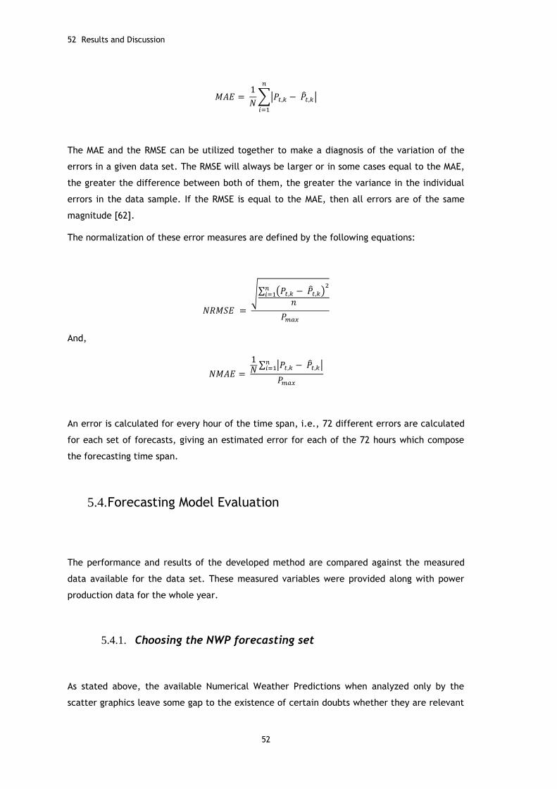
52 Results and Discussion
52
The MAE and the RMSE can be utilized together to make a diagnosis of the variation of the
errors in a given data set. The RMSE will always be larger or in some cases equal to the MAE,
the greater the difference between both of them, the greater the variance in the individual
errors in the data sample. If the RMSE is equal to the MAE, then all errors are of the same
magnitude [62].
The normalization of these error measures are defined by the following equations:
And,
An error is calculated for every hour of the time span, i.e., 72 different errors are calculated
for each set of forecasts, giving an estimated error for each of the 72 hours which compose
the forecasting time span.
5.4. Forecasting Model Evaluation
The performance and results of the developed method are compared against the measured
data available for the data set. These measured variables were provided along with power
production data for the whole year.
5.4.1. Choosing the NWP forecasting set
As stated above, the available Numerical Weather Predictions when analyzed only by the
scatter graphics leave some gap to the existence of certain doubts whether they are relevant
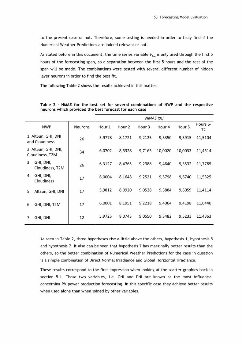
53 Forecasting Model Evaluation
to the present case or not. Therefore, some testing is needed in order to truly find if the
Numerical Weather Predictions are indeed relevant or not.
As stated before in this document, the time series variable is only used through the first 5
hours of the forecasting span, so a separation between the first 5 hours and the rest of the
span will be made. The combinations were tested with several different number of hidden
layer neurons in order to find the best fit.
The following Table 2 shows the results achieved in this matter:
Table 2 - NMAE for the test set for several combinations of NWP and the respective neurons which provided the best forecast for each case
NMAE (%)
NWP Neurons Hour 1 Hour 2 Hour 3 Hour 4 Hour 5 Hours 6-
72
1. AltSun, GHI, DNI and Cloudiness
26 5,9778 8,1721 9,2125 9,5350 9,5915 11,5104
2. AltSun, GHI, DNI, Cloudiness, T2M
34 6,0702 8,5328 9,7165 10,0020 10,0033 11,4514
3. GHI, DNI, Cloudiness, T2M
26 6,3127 8,4765 9,2988 9,4640 9,3532 11,7785
4. GHI, DNI, Cloudiness
17 6,0004 8,1648 9,2521 9,5798 9,6740 11,5325
5. AltSun, GHI, DNI 17 5,9812 8,0920 9,0528 9,3884 9,6059 11,4114
6. GHI, DNI, T2M 17 6,0001 8,1951 9,2218 9,4064 9,4198 11,6440
7. GHI, DNI 12 5,9725 8,0743 9,0550 9,3482 9,5233 11,4363
As seen in Table 2, three hypotheses rise a little above the others, hypothesis 1, hypothesis 5
and hypothesis 7. It also can be seen that hypothesis 7 has marginally better results than the
others, so the better combination of Numerical Weather Predictions for the case in question
is a simple combination of Direct Normal Irradiance and Global Horizontal Irradiance.
These results correspond to the first impression when looking at the scatter graphics back in
section 5.1. Those two variables, i.e. GHI and DNI are known as the most influential
concerning PV power production forecasting, in this specific case they achieve better results
when used alone than when joined by other variables.
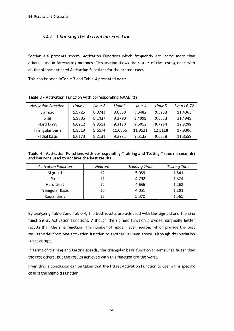
54 Results and Discussion
54
5.4.2. Choosing the Activation Function
Section 4.6 presents several Activation Functions which frequently are, some more than
others, used in forecasting methods. This section shows the results of the testing done with
all the aforementioned Activation Functions for the present case.
This can be seen inTable 3 and Table 4 presented next:
Table 3 - Activation Function with corresponding NMAE (%)
Activation Function Hour 1 Hour 2 Hour 3 Hour 4 Hour 5 Hours 6-72
Sigmoid 5,9725 8,0743 9,0550 9,3482 9,5233 11,4363
Sine 5,9805 8,1437 9,1790 9,4999 9,6553 11,4949
Hard Limit 6,0912 8,3512 9,3130 9,6012 9,7964 12,3289
Triangular basis 6,9319 9,6674 11,0856 11,9521 12,3118 17,9306
Radial basis 6,0173 8,2131 9,2271 9,5132 9,6218 11,8659
Table 4 - Activation Functions with corresponding Training and Testing Times (in seconds) and Neurons used to achieve the best results
Activation Function Neurons Training Time Testing Time
Sigmoid 12 5,039 1,361
Sine 11 4,792 1,324
Hard Limit 12 4,656 1,262
Triangular Basis 10 4,051 1,201
Radial Basis 12 5,370 1,565
By analyzing Table 3and Table 4, the best results are achieved with the sigmoid and the sine
functions as Activation Functions. Although the sigmoid function provides marginally better
results than the sine function. The number of hidden layer neurons which provide the best
results varies from one activation function to another, as seen above, although this variation
is not abrupt.
In terms of training and testing speeds, the triangular basis function is somewhat faster than
the rest others, but the results achieved with this function are the worst.
From this, a conclusion can be taken that the fittest Activation Function to use in this specific
case is the Sigmoid Function.

55 Forecasting Model Evaluation
5.4.3. Forecasting Results
As seen in the previous sections for the case of study of the present thesis, the best
combination of Numerical Weather Predictions is the use of Global Horizontal Irradiance and
Direct Normal Irradiance and the best Activation Function is the sigmoid function.
Thus, the following results were obtained with the use of aforementioned combination of
variables. One particularity of the developed method is that it trains a network for each hour
of the time span, and also it can start from whatever hour is chosen. The following examples
start at different times of the day; the first two samples start at 00:00 UTC and the
subsequent two start at 9.00 UTC for the 72 hour span. For the cases starting at 9:00 UTC the
span does not cover the expected 72 hour span because no data is available past the third
day of forecasting.
Figure 5.10 - Forecast made for April's 29th at 00:00 UTC for the next 3 days
Figure 5.10 shows a forecast made for April’s 29th at 00:00 UTC for the next 3 days. In this
figure the forecast’s error is by excess, i.e. the forecasted values are greater than the
measured values, when analyzing the NWP available for this horizon, the forecasted variables
(DNI and GHI) are substantially higher than the measured ones, which leads to this error. This
can be observed in Figure 5.11:

56 Results and Discussion
56
Figure 5.11 – Irradiation forecasting error for the span of April's 29th to May's 1st
Figure 5.12 - Forecast made for August’s 20th at 00:00 UTC for the next 3 days
Figure 5.12 shows a forecast made for August’s 20th at 00:00 UTC for the next 3 days. This
time span represents summer days with clear sky, and the forecast provides an almost null
error, a small divergence can be seen in the forecast for August’s 22nd, in which the produced
power peaks a little higher than the forecast. This can be explained by analyzing the previous
days, once the forecasting model utilizes series of past values and the previous day’s peak is
lower than in that day.
The next set of figures will show forecasts starting at 9:00 UTC:

57 Forecasting Model Evaluation
Figure 5.13 - Forecast made for April's 3rd at 9:00 UTC for the next three days
Figure 5.13 shows a forecast made for April’s 3rd for the next 3 days, starting at 9:00 UTC. In
this case, the NWP present a negative error, i.e. the NWP are lower than the measured
values, mostly for the second half of the day which leads to the graphic seen above. The
error can be observed in Figure 5.14:
Figure 5.14 – Irradiation forecasting error for the span of April's 3rd to April's 5th

58 Results and Discussion
58
Figure 5.15 - Forecast made for December’s 4th at 9:00 UTC for the next three days
Figure 5.15 shows a forecast made for December’s 4th for the next 3 days, starting at 9:00
UTC. The choice of the 9:00 UTC hour relates to the hour of opening of the power trade
market, in this case the MIBEL. One again, the NWPs have a relatively high error which
affects the final results of the forecasting. Figure 5.16 shows the NWP error:
Figure 5.16 – Irradiation forecasting error for the span of December's 4th to December's 6th
The figures above show that, as expected, in clear sky days, when the solar irradiance does
not vary too much, the achieved results are fairly good, but when the solar irradiance shows
some oscillation the forecast gets worse.

59 Forecasting Model performance
5.5. Forecasting Model performance
Apart from the original hybrid ELM model proposed for this thesis, in order have a better
perception over the achieved results, a comparison with a purely Autoregressive model
(which do not use NWP) and an ELM model using only NWP data.
The achieved results can be seen below:
Figure 5.17 - NMAE vs. Forecasting Horizon for the Hybrid ELM model
Figure 5.18 - NMAE vs. Forecasting Horizon for Autoregressive ELM model

60 Results and Discussion
60
Figure 5.19 - NMAE vs. Forecasting Horizon for the NWP ELM model
Figure 5.17 shows the NMAE of the hybrid model, the error is lower for the 5 first hours due
to the use of past time series, as stated previously.
Figure 5.18 shows the error values for the autogressive model, when comparing with the
hybrid model, it is noticeable that the shape of the graphic is identical, but the error is
higher, this is due to the use of NWP in the hybrid model, which lowers the error.
Figure 5.19 shows the NMAE when using only NWP with the ELM model, once the series of past
values are not used in this model, the input for the model do not differ much from each
other, thus, the low variation of the error for the whole span of time, i.e. the difference
between the higher error and the lower is very small being this difference observed in the
first hours of the time span. From this one can deduce that for the first hours of the time
span, the series of past values are more important than the NWP.
5.6. Comparison with other Methods
This section presents a comparison between the Extreme Learning Machines proposed model,
and Artificial Neural Networks and Support vector Machines.
Table 5 shows the test errors obtained with the same data set for the different methods. The
ELM developed method provided better results than the other two methods. The ANN is
slightly worse than the ELM; The ANN was trained and tested with the Levenberg-Marquardt
algorithm with Mat Lab. For the SVM the Mat Lab library LIBSVM was used, once it does not
possess any native function for this method. The worst results were obtained by the SVM
model. The present results are the mean of 50 runs of each model.

61 Comparison with other Methods
Table 5 - NMAE (in percentage) for the referred statistical models
Method Hour 1 Hour 2 Hour 3 Hour 4 Hour 5 Hours 6-72
ELM 5,9725 8,0743 9,0550 9,3482 9,5233 11,4363
ANN 6,3472 8,9305 8,7815 9,3619 9,5729 11,9463
SVM 8,1652 10,0673 10,6902 11,1738 10,4920 12,2741
In terms of speed, the ELM is much faster than the other two models; Table 6 shows the
times for one run of each model in an Intel Core i7 Q720 @ 1.60 GHz with 8GB of RAM:
Table 6 - Training and Testing times of the statistical methods (in seconds)
Method Training Time Testing Time
ELM 5.039 1.361
ANN 15.929 1.3731
SVM 37.147 7.941
As seen above, the Extreme Learning Machines model achieves very good performances even
when comparing with other statistical methods. Most glaringly is its speed which completely
overwhelms the other models.
The errors can be graphically seen below in Figure 5.20 and Figure 5.21:
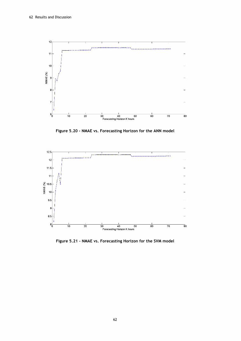
62 Results and Discussion
62
Figure 5.20 - NMAE vs. Forecasting Horizon for the ANN model
Figure 5.21 - NMAE vs. Forecasting Horizon for the SVM model


Chapter 6
Conclusion
Although the Photovoltaic energy production has not yet an expressive share when compared
to traditional sources, it is estimated, as seen previously, that it will rise in importance in the
coming years. This kind of energy has insurmountable capabilities to explore, and is the
biggest source of energy mankind has access to. Also, the continuous pressures of
environmental institutions backed by Kyoto’s protocol, makes it a priority to develop and
increase the use of renewable energies. Thus, power production forecasting is increasingly
gaining importance, as a tool to improve the control capability and usability of these
energies, once they are very intermittent and hard to predict.
The main objective of the present thesis was to develop a new and innovative forecasting
method, for short-term photovoltaic forecasting, in this case for a span of 72 hours ahead.
The main conclusions are presented next.
A method for photovoltaic power production forecasting has been developed using a
relatively new technology called Extreme Learning Machines. The developed method
forecasts the photovoltaic power production for the next 72 hours, and a forecast is made for
each hour of the span, i.e. 72 different networks were trained and tested. One particularity
of the present method is the capability of varying the starting hour of the forecast, i.e. it can
start at 0:00 UTC or at 9:00 UTC or at which hour it is preferred or suits better the user.
The method focused on Extreme Learning Machines algorithms analyzed three different
forecasting models: One using only data of production past values, i.e. purely autoregressive;
another using only Numerical Weather Predictions; and the last one being a hybrid model
between the two previously referred models, i.e. using series of past values and NWP. The
conclusion was that the hybrid model provides better results, which infers that the use of
NWP enhances the results and thus, they add value to the forecasting model.
Also, several NWP variables were tested in order to find the best combination for the present
method. The available variables were temperature 2 meters above ground, direct normal

65 Future Works
irradiance, global horizontal irradiance, cloudiness and solar altitude. It was found that the
minimum forecasting error was obtained when a conjugation of direct normal irradiance and
global horizontal irradiance was used.
Several activation functions were also tested with the developed model and the best results
were achieved when using the sigmoid function.
The developed model was also tested against other statistical models, e.g. ANN and SVM, and
better results were achieved when using the same data sets for each model. The ANN obtains
slightly worse results than the ELM, while the SVM is clearly the less reliable model in this
case. Also, one important feature of the Extreme Learning Machines relating to other
methods is its learning speed, which overwhelms the other models. Learning speed is very
important characteristic for forecasting models, once it very important that the forecast are
ready before the opening of the markets, and thus, the forecasts cannot take too much time
to be done.
The available data set for this thesis covers only the span of one year (2010), which is not
ideal for this kind of work. To try to lessen the influence of this detail, the training and
testing sets were rearranged in order to avoid training the model with mostly summer and
spring months and testing with autumn and winter months.
The objectives of the proposed thesis were entirely covered and fulfilled. A forecasting
model of Extreme Learning Machines using a hybrid combination of series of past values and
NWP was develop and tested, and the results were found fairly good, reaching an error below
6% for the first hour and steadily rising to around 9% for the following 4 hours, once they use
series of past power production values as input, for the span of the hours 6-72 the Numerical
Weather Predictions were found to be a more relevant input with an error always rounding
11%. Nevertheless further work can be done to improve the model.
6.1. Future Works
For future works some possibilities are presented:
Calculation of the diffuse radiation in order to add more precision to the
method;
Calculation of the temperature of the PV module from the ambient
temperature;

Conclusion
66
Using other NWP variables as input in order to test their influence, e.g. wind
speed or wind direction could be of influence;
The creation of an user interface could also had value to the developed method
once it would be easier to use;
Data of several years could be used in order to find a better characterization of
seasonal periodicity.

Bibliography
[1] Bacher, Peder, “Online Short-term Solar Power Forecasting”, Solar Energy 83, 1772-1783
Accessed in September 2013.
[2] Neves, Ricardo, “Desenvolvimento de modelos de previsão de produção de centrais
fotovoltaicas”. Accessed in September 2013.
[3] http://www.ntu.edu.sg/home/egbhuang/ , Accessed in September 2013
[4] http://cleantechnica.com/2013/10/08/advantages-disadvantages-solar-power/ ,
Accessed in October 2013
[5] http://www.erse.pt , Accessed in October 2013
[6] http://expresso.sapo.pt/renovaveis-abastecem-portugal-de-eletricidade=f797507,
Accessed in October 2013
[7] http://www.indexmundi.com/blog/index.php/2013/08/07/china-at-the-top-of-
renewable-energy-investment/ October 2013
[8] http://www.carbonbrief.org/blog/2013/01/renewable-investment-drops-2012/, Accessed
in October 2013
[9] http://cleantechnica.com/2013/07/12/solar-pv-to-hit-grid-parity-134-billion-annual-
revenue-by-2020/, Accessed in October 2013
[10] http://www.3tier.com/en/support/resource-maps/, Accessed in October 2013
[11] Monteiro, Cláudio, “Previsão de Consumos – O problema da previsão de consumos”,
Available in http://paginas.fe.up.pt/~cdm/DE2/DE2_A3a.pdf , Accessed in October 2013
[12] Sousa, João, http://www.slideshare.net/CongressoEnergiaViana/joo-sousa-prewind ,
Accessed in October 2013
[13] http://www.cmhc-schl.gc.ca/en/co/grho/grho_009.cfm , Accessed in October 2013
[14] http://www.fsec.ucf.edu/en/consumer/solar_electricity/basics/how_pv_system_works.h
tm , Accessed in October 2013
[15] Centro de Referência para Energia Solar e Eólica Sérgio de Salvo Brito, "Energia Solar -
Princípios e Aplicações"., Accessed in October 2013
[16] “Energia Fotovoltaica – Manual sobre tecnologias”, projecto e instalação,
http://www.jgduarte.com/download/greenpro_fotovoltaico.pdf, Accessed in October
2013
[17] http://www.yourhome.gov.au/technical/fs67.html, Accessed in October 2013
[18] Hyndman, Rob J., Athanasopoulos, George, “Forecasting: Principles and practice”,
http://www.otexts.org/book/fpp, Accessed in October 2013
[19] Sfetsos, A., Coonick, A.H., “Univariate and Multivariate Forecasting of Hourly Solar
Radiation With Artificial Intelligence Techniques”, Solar Energy, 2000. 68(2) p.129-134,
Accessed in November 2013

68
[20] Box, George E.P.; Jenkins, Gwimly M.; Reinsel, Gregory C., “Time Series Analysis:
Forecasting Control”, Prentice-Hall Inc., Accessed in November 2013
[21] Heineman, Detlev; Lorenz, Elke; Girodo, Marco; “Forecasting of Solar Radiation”, Solar
Energy 67, 139-150, Accessed in November 2013
[22] Wu, Ji; Chan, Chee Keong; “Prediction of hourly solar radiation using a novel hybrid
model of ARMA and TDNN”, Accessed in November 2013
[23] Heineman, Detlev; Lorenz, Elke; Girodo, Marco; “Solar irradiance forecasting for the
management of solar energy systems”, Solar 2006, Denver, CO, USA, Accessed in
November 2013
[24] Silva, Carlos, “Desenvolvimento de uma metodologia e ferramentas para a previsão da
produção elétrica em parques fotovoltaicos”, Accessed in November 2013
[25] Zhang, G et al.,”Forecasting with artificial neural networks”, Accessed in November
2013
[26] Krogh, Anders, “What are artificial neural networks”, Available in
http://www.apl.jhu.edu/~przytyck/neural_net_primer.pdf, accessed in November 2013
[27] http://www.learnartificialneuralnetworks.com/ , Accessed in November 2013
[28] Aamodt, Rune, “Using artificial networks to forecast financial time series”, Available in
http://www.diva-portal.org/smash/get/diva2:353048/FULLTEXT01.pdf, Accessed in
November 2013
[29] http://iticsoftware.com/forex-neural-backpropagation, Accessed in November 2013
[30] http://upload.wikimedia.org/wikipedia/commons/7/73/AtmosphericModelSchematic.png
, Accessed in November 2013
[31] http://reference.wolfram.com/applications/neuralnetworks/NeuralNetworkTheory/2.5.1
.html, Accessed in November 2013
[32] http://www.roguewave.com/portals/0/products/imsl-numerical-libraries/c-
library/docs/7.0/html/cstat/default.htm?turl=multilayerfeedforwardneuralnetworks.htm
, Accessed in November 2013
[33] Joachims, Thorsten, “Text categorization with support vector machines: Learning with
many relevant features”, Available in
http://link.springer.com/chapter/10.1007/BFb0026683#page-1, Accessed in November
2013
[34] Basak, Debasish et al., “Support Vector Regression”, Available in
http://pdf.aminer.org/000/260/306/position_control_of_ultrasonic_motor_using_support
_vector_regression.pdf, Accessed in November 2013
[35] Hammer, A. et al., “Solar energy assessment using remote sensing techniques”, Remote
Sensing of Environment 86, 423-432, 2003, Accessed in January 2013
[36] Huang,Guang-Bin, Siew, Chee-Kheong, ”Extreme learning Machine with Randomly
Assigned RBF Kernels”, International Journal of Information Technology, Vol. 11, No. 1,
pp: 16-24, 2005. Accessed in November 2013

69
[37] Huang, G.; Zhou, H.; Ding,X.; et al.; “Extreme Learning Machines for regression and
multiclass classification.”, Accessed November 2013
[38] Liu, Quige; He, Qing; Shi, Zhongzhi; “Extreme Support Vector Machine Classifier”,
Accessed in December 2013
[39] Huang, G.; Zhu, Q.; Siew, C.; “Extreme Learning Machine: Theory and applications”,
Neurocomputing, Vol. 70, pp: 489-501, 2006 Accessed in December 2013
[40] Frénay, Benoît; Verleysen, Michel; “Using SVMs with randomized feature spaces an
extreme learning approach”, Accessed in December 2013
[41] Suykens, J.A.K.; Vandewalle, J.; “Training multilayer perceptron classifiers based on a
modified support vector method”, Accessed in December 2013
[42] Huang, G.; Zhou, H.; Ding,X.; “Optimization method based extreme learning machine for
classification”,Accessed in December 2013
[43] Bartlett, P.L.; “ The sample complexity of pattern classification with neural networks:
The size of the weights is more important than the size of the network”, Accessed in
December 2013
[44] http://www.3tier.com/en/support/solar-prospecting-tools/what-global-horizontal-
irradiance-solar-prospecting/, Accessed in December 2013
[45] http://pvpmc.org/modeling-steps/irradiance-and-weather-2/irradiance-and-
insolation/global-horizontal-irradiance/, Accessed in December 2013
[46] http://www.brighton-webs.co.uk/energy/solar_horizontal_surface.aspx, Accessed in
December 2013
[47] http://www.bom.gov.au/climate/austmaps/solar-radiation-glossary.shtml, Accessed in
December 2013
[48] http://www.3tier.com/en/support/solar-prospecting-tools/what-direct-normal-
irradiance-solar-prospecting/, Accessed in December 2013
[49] Dai, Aiguo, et al.; “Recent trends in cloudiness over the united states: A tale of
monitoring inadequencies”, Available in
http://www.cgd.ucar.edu/cas/adai/papers/Dai_etal_BAMS_Clouds.pdf, Accessed in
December 2013
[50] Mantzari, Vassilili H.; Mantzaris, Dimitrios H.; “Solar Radiation: Cloudiness forecasting
using a soft computing approach”, Accessed in December 2013
[51] http://pveducation.org/pvcdrom/properties-of-sunlight/elevation-angle, accessed in
December 2013
[52] Soteris A, K., “Applications of artificial neural-networks for energy systems. Applied
Energy”, Applied Energy, 2000. 67(1-2): p. 17-35, Accessed in December 2013
[53] Ogliari, E., et al., “Hybrid Predictive Models for Accurate Forecasting in PV Systems”, Accessed in December 2013

70
[54] Yona, A.; Senjyu, T.; Saber, A.Y.; Funabashi, T.; Sekine, H.; Kim, C.-H. “Application of
Neural Network to One-day-ahead 24 hours Generating Power Forecasting for
Photovoltaic System.”, Accessed in December 2013
[55] Zeng, J; Qiao, W; “Short-term solar power prediction using a support vector machine”,
Accessed in December 2013
[56] Huang, G et al.; “Extreme Learning Machine: A New Learning Scheme of Feedforward
Neural Networks”, International Joint Conference on Neural Networks, Vol. 2, pp: 985-
990, 2004, Accessed in December 2013
[57] “The Moore-Penrose pseudo-inverse”, Available in
http://robotics.caltech.edu/~jwb/courses/ME115/handouts/pseudo.pdf, Accessed in
December 2013
[58] “Neural activation functions”, Available in
http://staff.science.uva.nl/~leo/math/sigma.pdf, Accessed in December 2013
[59] I.S.Isa, Z.Saad, S.Omar, M.K.Osman, K.A.Ahmad, H.A.Mat Sakim, “Suitable MLP Network
Activation Functions for Breast Cancer and Thyroid Disease Detection”, Accessed in
December 2013
[60] Bekir Karlik, A. Vehbi Olgac; “Performance Analysis of Various Activation Functions in
Generalized MLP Architectures of Neural Networks”, Accessed in December 2013
[61] Muhammad Taher Abuelma'Att, Abdullah Bakri Shwehneh; "A Reconfigurable
Gaussian/triangular Basis Functions Computation Circuit”, Accessed in December 2013
[62] http://www.eumetcal.org/resources/ukmeteocal/verification/www/english/msg/ver_co
nt_var/uos3/uos3_ko1.htm, Accessed in December 2013
[63] B. H. Chowdhury and S. Rahman, "Forecasting sub-hourly solar irradiance for prediction of
photovoltaic output", in Conference Record of the IEEE Photovoltaic Specialists
Conference, pp. 171-176, (1987), Accessed in December 2013
[64] S. Hokoi, et al., "Stochastic models of solar radiation and outdoor temperature", in
ASHRAE Transactions Vol. 2, pp.245-252, Accessed in December 2013
[65] Mathiesen and Kleissl, “Evaluation of numerical weather prediction for intra-day solar
forecasting in the continental United States”, Solar Energy 85 (5), 967-977, Accessed in
December 2013
[66] Claudio Monteiro et al., “Short-Term Power Forecasting Model for Photovoltaic Plants
Based on Historical Similarity”, Accessed in December 2013~
[67] Diagne et al., “solar irradiation forecasting: state of the art and proposition for future
developments for small-scale insular grids”, Accessed in December 2013
[68] Paoli et al., “ Forecasting of preprocessed daily solar radiation time series using neural
networks”, Solar Energy 84 (12), 2146-2160 Accessed in December 2013
[69] Mellit, Adel; Pavan, A.M.; “A 24h forecast of solar irradiance using artificial neural
network: Application of performance prediction of a grid-connected PV plant at Trieste,
Italy”, Solar Energy 84 (5), 807-821, Accessed in December 2013

71
[70] Lorenz, E., et al.; “Irradiance forecasting for the power prediction of grid-connected
photovoltaic system”, IEEE Journal of Selected Topics in Applied Earth Observations and
remote sensing, Vol. 2, No. 1, March 2009, Accessed December 2013
[71] http://science.howstuffworks.com/dictionary/physics-terms/heat-info3.htm, Accessed in
December 2013
[72] Kwok, J.T.Y.;”Support Vector Mixture for Classification and Regression Problems”,
Accessed in December 2013
[73] Rajesh, R.; Prakash, J.S.;”Extreme Learning Machines – A Review and State-of-the-Art”,
Accessed in December 2013
[74] Reikard, G.;”Predicting Solar Radiation at High Resolutions: A Comparison of Time Series
Forecasts”, Solar Energy 83 (3), 342-349, Accessed in December 2013
[75] Hamilton, J.D.;”Time Series Analysis” Princeton University Press, 1994, Accessed in
December 2013
[76] Remund et al.;”Comparison of solar radiation forecasts for the USA”, Solar Radiation at
High Resolutions: A Comparison of Time Series Forecasts”, USA. Proc. of the 23rd
European PV Conference, 1.9-4.9 2008, Valencia, Spain Accessed in December 2013
[77] Perez et al.;”Validation of short and medium term operational solar radiation forecasts in
the US”, Solar Energy 84 (5) 2161-2172, Accessed in December 2013
[78] Cao and Cao;”Forecast of solar irradiance using recurrent neural networks combined with
wavelet analysis”, Energy 31, 3435-3445 (2006), Accessed in December 2013
[79] Lorenz et al.;”Benchmarking of different approaches to forecast solar irradiance”, In:
Proceedings of 24 European Photovoltaic and Solar Energy Conference and Exhibition,
Hamburg (Germany), Accessed in December 2013
[80] http://www.altenergystocks.com/archives/2012/04/five_more_winners_of_the_clean_en
ergy_race_1.html , Accessed in January 2014

72
Appendixes
Appendix A
Clear Sky Model
The clear sky model used in this work was inspired by the one proposed by Bacher [1].
A clear sky model is normally a model which estimates the global irradiance in clear sky at
any given time. Chowdhury and Rahman [63] divide the global irradiance into a clear sky
element and a cloud cover element by:
Where G is the global irradiance in W/m2, is the clear sky global irradiance in W/m2 and
is the transmissivity of the clouds which they model as a stochastic process using ARIMA
models. The clear sky global irradiance is found by
Where is the extraterrestrial irradiance in W/m2 and is the total sky transmissivity in
clear sky, which is modeled by atmospheric dependent parametrization.
In the study proposed by Bacher [1], an identical approach is made, although instead of
applying the factor on global irradiance it is applied to solar power, i.e.
Where p is the solar power in W, is the clear sky power in W and is much like but
since the clear sky model developed by Bacher [1] estimates by statistical smoothing

73
techniques rather than physics, the method can be mainly viewed as a statistical
normalization technique and is then referred to as normalized solar power.
The main motivation behind this normalization of solar power with a clear sky model is that
normalized solar power is more stationary than the solar power, so that classical time series
models assuming stationarity can be used for predicting the normalized values.
The clear sky model is defined as:
Where is the clear sky solar power in W, x is the day of the year and y is the time of the
day. The function is assumed to be a smooth function and thus, can be estimated as
a local maximum. The estimated clear sky function is then used to form the output
of the clear sky model as the time series
Where is the estimated clear sky solar power in W at time t and N is the number of hours
of the time series. The normalized solar power Is then defined as
And this is used to form time series of normalized solar power.
For each (x,y) corresponding to the solar power observation , weighted quantile regression
estimates q quantile by a Gaussian two-dimensional smoothing kernel. The smoothing kernel
is used to form the weights applied in the quantile regression. The applied weights are finally
found by multiplying the weights from the two dimensions. The choice of quantile level q to
be estimated and the bandwidth in each dimension, and , is based on a visual inspection
of the results. A level of q = 0.85 was used.
For small values, the error of is naturally increasing and at nighttime the error is
infinite. Therefore, all values of where
Are removed from { }. is the maximum value of the
series.
The estimates of clear sky solar power are comprehensibly better in the summer period. The
bad estimates in the winter periods are caused by the sparse number of clear sky
observations.
It is noted that the deterministic changes of solar power are really caused by the geometric
relation between the earth and the sun, which can be represented by the sun elevation as x
and the sun azimuth as y.

74

75
Appendix B
Moore-Penrose generalized inverse matrix
The Moore-Penrose pseudo-inverse is a general way of finding a solution to the subsequent
system of linear equations:
Moore and Penrose showed that there is a general solution for the latter equation system of
the form of . The matrix is the Moore-Penrose pseudo-inverse, and it was proved
that is the unique matrix capable of satisfying the following properties:
A A =A;
A = ;
= A ;
= .
The Moore-Penrose pseudo-inverse has the following properties:
m=n, if A is full rank. The pseudo-inverse for the case where A is not full rank
will be considered below.
m>n, the solution is the one capable of minimizing the quantity:
That is, in this case there are more constraints than free variables y. Hence, it is
generally impossible to find a solution to these equations. This pseudo-inverse gives
the solution y, so that y is closest (in a LS (Least Squared) sense) to the desired
solution for vector b.

76
m<n, then the Moore-Penrose solution minimizes the 2-norm of y: . In this case,
there exists, generally, an infinite number of acceptable solutions, and the Moore-
Penrose solution is the particular solution in which the vector 2-norm is minimal.
However, when A is not full rank, then these formulas cannot be used [57].