faculty of industrial engineering, mechanical engineering and

Faculty of Industrial Engineering,Mechanical Engineering and Computer Science

University of Iceland2013


University of Iceland2013

Utilization of absorption cycles forNesfiskur and Skinnfiskur

Þorsteinn Hauksson

UTILIZATION OF ABSORPTION CYCLES FORNESFISKUR AND SKINNFISKUR

Þorsteinn Hauksson

30 ECTS thesis submitted in partial fulfillment of aMagister Scientiarum degree in Mechanical Engineering

AdvisorDr. Halldór Pálsson, Associate Professor, University of Iceland

Dr. Magnús Þór Jónsson, Professor, University of Iceland

Faculty RepresentativeDr. Páll Valdimarsson, University of Iceland


School of Engineering and Natural SciencesUniversity of IcelandReykjavik, July 2013

Utilization of absorption cycles for Nesfiskur and Skinnfiskur30 ECTS thesis submitted in partial fulfillment of a M.Sc. degree in MechanicalEngineering

Copyright c© 2013 Þorsteinn HaukssonAll rights reserved

Faculty of Industrial Engineering,Mechanical Engineering and Computer ScienceSchool of Engineering and Natural SciencesUniversity of IcelandSæmundargötu 2101, ReykjavikIceland

Telephone: 525 4000

Bibliographic information:Þorsteinn Hauksson, 2013, Utilization of absorption cycles for Nesfiskur and Skinnfiskur,M.Sc. thesis, Faculty of Industrial Engineering,Mechanical Engineering and Computer Science, University of Iceland.

Printing: Háskólaprent, Fálkagata 2, 107 ReykjavíkReykjavik, Iceland, July 2013

Abstract

Refrigeration systems are well known in industry and households. The purpose of suchsystem may include a variety of tasks. In our daily lives we use refrigerators and freezersto keep food cold or frozen. Large fisheries in Iceland use mainly compressor systems tofreeze fish for conservation, although this technology may not be the most cost effective.This thesis emphasizes on how to utilize absorption refrigeration technologies in Icelandand use optimization to investigate specific cases which are dealt with. This is done tofind out whether companies can save equity by using unused heat from geothermal powerplants or other heat source.The main conclusion from the thesis is that absorption systems are not economical forthe companies Skinnfiskur and Nesfiskur when compared to compressor system in termsof three cases that are discussed. The initial cost for the absorption system is too high.In case A the pipeline is too long and the pressure drop high, therefore the cost is toohigh. In case B the pipeline is not as long as in case A but the flow in the pipes is highwhich means larger diameter of the pipe and the cost increases dramatically which meansthat the case is not profitable. Case C is the most favorable of the three cases but not asprofitable as current system.

Útdráttur

Kælikerfi eru vel þekkt í iðnaði og í heimilum. Tilgangur kælingar getur verið margskonar.Í daglegu lífi notum við ísskápa og frysta til að viðhalda mat köldum eða frystum. Stórútgerðarfyrirtæki á Íslandi nota aðallega þjöppur til að frysta fisk sem er síðan fluttur ífrystigeymslur. Þessi tækni þarf ekki endilega að vera hagkvæmust.Í þessari ritgerð er athugað hvernig skal nýta ísogs tækni á Íslandi til þess notuð bestunfyrir hvert tilfelli sem er fjallað um. Þetta er gert til að finna hvort fyrirtæki geta sparað fémeð því að nota ónýttan hita frá jarðvarmavirkjunum eða öðrum varmagjöfum.Helsta niðurstaða ritgerðarinnar er sú að ísogskerfi eru ekki hagkvæm fyrir fyrirtækinSkinnfisk og Nesfisk þegar þau eru borin saman við þjöppunarkerfi í þeim tilvikum semfjallað erum, fjárfestingarkostnaðurinn er of hár. Í tilfelli A er pípulögnin of löng ogþrýstingstapið mikið á leiðinni, þar af leiðandi er kostnaðurinn of hár. Í tilfelli B erpípulögnin ekki eins löng og í tilfelli A en flæðið í pípunni er mikið sem þýðir að þvermálpípunnar er meira og eykst þá pípu kostnaðurinn verulega, sem þýðir að verkefnið erekki arðbært. Tilfelli C er hagstæðast af öllum þrem tilfellunum en ekki eins hagstætt ognúverandi kerfi.

Contents

List of Figures ix

List of Tables xi

Abbreviations xiii

Acknowledgments xv

1. Introduction 1

2. Theory of refrigeration systems 32.1. Working cycles . . . . . . . . . . . . . . . . . . . . . . . . . . . . . . . 3

2.1.1. Compressor system . . . . . . . . . . . . . . . . . . . . . . . . . 32.1.2. Single stage absorption systems . . . . . . . . . . . . . . . . . . 52.1.3. Two stage absorption system . . . . . . . . . . . . . . . . . . . . 62.1.4. Comparison between compressor and absorption system . . . . . 7

2.2. Working fluids . . . . . . . . . . . . . . . . . . . . . . . . . . . . . . . . 72.3. COP found from fish muscle . . . . . . . . . . . . . . . . . . . . . . . . 82.4. Methodology for the calculations in the problem . . . . . . . . . . . . . . 102.5. Absorption model . . . . . . . . . . . . . . . . . . . . . . . . . . . . . . 12

2.5.1. Model of a single stage absorption cycle . . . . . . . . . . . . . . 122.5.2. Optimization . . . . . . . . . . . . . . . . . . . . . . . . . . . . 16

3. Case studies and results 173.1. HS veitur . . . . . . . . . . . . . . . . . . . . . . . . . . . . . . . . . . 173.2. Description of the companies involved . . . . . . . . . . . . . . . . . . . 18

3.2.1. Nesfiskur ehf . . . . . . . . . . . . . . . . . . . . . . . . . . . . 183.2.2. Skinnfiskur ehf . . . . . . . . . . . . . . . . . . . . . . . . . . . 20

3.3. Case A - Pipeline from Reykjanes to Skinnfiskur and Nesfiskur . . . . . . 223.3.1. Nesfiskur . . . . . . . . . . . . . . . . . . . . . . . . . . . . . . 233.3.2. Skinnfiskur . . . . . . . . . . . . . . . . . . . . . . . . . . . . . 283.3.3. Cost estimation . . . . . . . . . . . . . . . . . . . . . . . . . . . 31

3.4. Case B - Use of a district heating system . . . . . . . . . . . . . . . . . . 353.4.1. Nesfiskur . . . . . . . . . . . . . . . . . . . . . . . . . . . . . . 383.4.2. Skinnfiskur . . . . . . . . . . . . . . . . . . . . . . . . . . . . . 393.4.3. Piping system and pressure drop . . . . . . . . . . . . . . . . . . 393.4.4. Cost estimation . . . . . . . . . . . . . . . . . . . . . . . . . . . 41

vii

3.5. Case C - Freezing plant . . . . . . . . . . . . . . . . . . . . . . . . . . . 433.5.1. Model and optimization . . . . . . . . . . . . . . . . . . . . . . 433.5.2. Cost estimation . . . . . . . . . . . . . . . . . . . . . . . . . . . 46

4. Conclusion 494.1. Pipeline from Reykjanes to Skinnfiskur and Nesfiskur . . . . . . . . . . . 494.2. Use of a district heating system . . . . . . . . . . . . . . . . . . . . . . . 494.3. Freezing Hotel . . . . . . . . . . . . . . . . . . . . . . . . . . . . . . . 50

5. Future work 51

References 53

Appendices 55

A. Tables and Figures 57A.1. Nesfiskur, Case A . . . . . . . . . . . . . . . . . . . . . . . . . . . . . . 57A.2. Skinnfiskur, Case A . . . . . . . . . . . . . . . . . . . . . . . . . . . . . 59A.3. Nesfiskur, Case B . . . . . . . . . . . . . . . . . . . . . . . . . . . . . . 61A.4. Skinnfiskur, Case B . . . . . . . . . . . . . . . . . . . . . . . . . . . . . 63A.5. Freezing plant, Case C . . . . . . . . . . . . . . . . . . . . . . . . . . . 65

B. Programs 67B.1. Assumptions - Integral . . . . . . . . . . . . . . . . . . . . . . . . . . . 67B.2. Programming for Case A . . . . . . . . . . . . . . . . . . . . . . . . . . 68B.3. Programming for Case B . . . . . . . . . . . . . . . . . . . . . . . . . . 74B.4. Programming for Case C . . . . . . . . . . . . . . . . . . . . . . . . . . 78B.5. Pressure drop . . . . . . . . . . . . . . . . . . . . . . . . . . . . . . . . 82

viii

List of Figures

2.1. Component diagram of a compressor system . . . . . . . . . . . . . . . . 4

2.2. T-s Diagram . . . . . . . . . . . . . . . . . . . . . . . . . . . . . . . . . 4

2.3. Basic absorption system . . . . . . . . . . . . . . . . . . . . . . . . . . 5

2.4. Double effect absorption system . . . . . . . . . . . . . . . . . . . . . . 6

2.5. Enthalpy difference in a fish muscle from 10− (−18)◦C. . . . . . . . . . . . 9

2.6. Absorption cycle . . . . . . . . . . . . . . . . . . . . . . . . . . . . . . . 13

2.7. Descriptive diagram of a H2O/NH3, single stage absorption system . . . . . . 15

3.1. Temperature range in a deep freezer at Nesfiskur ehf. . . . . . . . . . . . 18

3.2. Power usage in Nesfiskur for different time periods. . . . . . . . . . . . . 19

3.3. Reykjanes power plant after possible changes . . . . . . . . . . . . . . . 22

3.4. Pipeline from RPP to Skinnfiskur and Nesfiskur [Map taken from www.ja.is]. 23

3.5. Modified single stage absorption cycle for case A . . . . . . . . . . . . . . . 24

3.6. How evaporation power depends on pressure and the NH3 : H2O ratio. . . . . . 26

3.7. Heat exchange process for the desorber and absorber . . . . . . . . . . . 28

3.8. Modified District heating system . . . . . . . . . . . . . . . . . . . . . . 35

3.9. Pipeline from Vellir to Skinnfiskur and Nesfiskur . . . . . . . . . . . . . 35

3.10. Modified single stage absorption cycle for case B . . . . . . . . . . . . . . . 36

3.11. Modified of a two stage absorption cycle . . . . . . . . . . . . . . . . . . . . 44

ix

A.1. Heat exchange process in each heat exchanger in the absorption cycle . . 58

A.2. Heat exchange process in each heat exchanger in the absorption cycle atSkinnfiskur . . . . . . . . . . . . . . . . . . . . . . . . . . . . . . . . . 60

A.3. Heat exchange process in each heat exchanger in Nesfiskur, case B . . . . 62

A.4. Temperature profiles in each heat exchanger in Skinnfiskur, case B . . . . 64

A.5. Temperature profiles in each heat exchanger case C . . . . . . . . . . . . 66

x

List of Tables

2.1. Absorption system compared to compression system . . . . . . . . . . . 7

2.2. Determination of factor α . . . . . . . . . . . . . . . . . . . . . . . . . . 12

3.1. Electricity cost at Nesfiskur . . . . . . . . . . . . . . . . . . . . . . . . . 20

3.2. Power used by the freezers in Nesfiskur. . . . . . . . . . . . . . . . . . . 20

3.3. Other refrigeration systems that are not taken into consideration but couldbe replaced with an absorption system. . . . . . . . . . . . . . . . . . . . 20

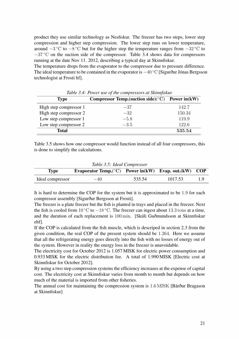
3.4. Power use of the compressors at Skinnfiskur. . . . . . . . . . . . . . . . . 21

3.5. Ideal Compressor . . . . . . . . . . . . . . . . . . . . . . . . . . . . . . 21

3.6. Optimization for the mass flow from RPP, case A - Nesfiskur . . . . . . . 25

3.7. Flow in different pipe diameters . . . . . . . . . . . . . . . . . . . . . . 26

3.8. Overall heat coefficient, area and energy consumption for heat exchangers- Case A, Nesfiskur . . . . . . . . . . . . . . . . . . . . . . . . . . . . . 27

3.9. Optimization for the mass flow from RPP - case A, Skinnfiskur . . . . . . 28

3.10. Flow in different pipe diameters - Skinnfiskur . . . . . . . . . . . . . . . 29

3.11. Overall heat coefficient, area and energy consumption of heat exchangers- Case A, Skinnfiskur . . . . . . . . . . . . . . . . . . . . . . . . . . . . 29

3.12. Pipe diameters - Skinnfiskur and Nesfiskur . . . . . . . . . . . . . . . . . 30

3.13. Estimate cost for components in case A - Nesfiskur . . . . . . . . . . . . 32

3.14. Estimate cost for components in case A - Skinnfiskur . . . . . . . . . . . 32

3.15. Breakdown of total capital investment, Case A . . . . . . . . . . . . . . . 33

xi

3.16. present value of an annuity for case A and current mechanism . . . . . . 34

3.17. Optimization for the mass flow from the district heating system - Case B,Nesfiskur . . . . . . . . . . . . . . . . . . . . . . . . . . . . . . . . . . 38

3.18. Area and energy consumption of the heat exchangers in - Case B, Nesfiskur 38

3.19. Optimization for the mass flow from the district heating system - Case B,Skinnfiskur . . . . . . . . . . . . . . . . . . . . . . . . . . . . . . . . . 39

3.20. Area and energy consumption of the heat exchangers at - Case B, Skinnfiskur 39

3.21. Chosen pipe diameters in case B . . . . . . . . . . . . . . . . . . . . . . 40

3.22. Estimate cost for components - Case B . . . . . . . . . . . . . . . . . . . 41

3.23. Breakdown of total capital investment, Case B . . . . . . . . . . . . . . . 42

3.24. PVOAA for case B and current mechanism . . . . . . . . . . . . . . . . 43

3.25. Optimization for the COP in a freeze plant next to the RPP - Case C . . . 45

3.26. Area and energy consumption of the heat exchangers in - Case C . . . . . 45

3.27. Breakdown of total capital investment, Case C . . . . . . . . . . . . . . . 46

3.28. PVOAA for case C and current mechanism . . . . . . . . . . . . . . . . 47

A.1. Properties for each point in case A at Nesfiskur . . . . . . . . . . . . . . 57

A.2. Properties for each point in case A at Skinnfiskur . . . . . . . . . . . . . 59

A.3. Properties for each point in case B at Nesfiskur . . . . . . . . . . . . . . 61

A.4. Properties for each point in case B at Skinnfiskur . . . . . . . . . . . . . 63

A.5. Properties for each point in case C . . . . . . . . . . . . . . . . . . . . . 65

xii

Abbreviations

Symbols and units of parameters

Symbol Dimension Description

A m2 Areaε m Roughnessd kg/m2 Densityh kJ/kg EnthalpyG l/s FlowL m Lengthm kg Massm kg/s Massflowη ... Efficiencyp Pa Pressurepf Pa Pressure loss∆pf Pa/m Pressure loss per meterρ kg/m3 DensityQ kJ EnergyQ kW Heatq ... Qualitys kJ/K EntropyT ◦C Temperature

U W/(m2 · ◦C) Overall heat transfercoefficient

v m3/kg Specific volumeW kW Work

x ...NH3 : H2O ratio in liquidphase

y ...NH3 : H2O ratio in vaporphase

xiii

Acknowledgments

This masters thesis would not have been possible without the support of many people.I would like to express my gratitude to my advisors Halldór Pálsson and Magnús ÞórJónsson for their guidance trough this project. I would also like to express my appreciationto the staff at HS-Orka, Skinnfiskur and Nesfiskur. Finally, special thanks to to my familyand to my friends who have supported me socially and mentally during this project.

xv

1. Introduction

Refrigeration systems are widely used in homes and in industrial applications. They are ofvarious type, with various efficiencies and of different sizes. In all cases there is a need toexamine different options when designing a refrigeration system. In homes, refrigerationsystems are mainly used to preserve food, cooled or frozen, and also for air conditioning.In industry, refrigeration systems are used in larger applications such as air conditioningsystems for hospitals and warehouses, refrigeration for large storage rooms with foodproducts and some fisheries need to quickly freeze fish to a low temperature.When the temperature is slightly above the freezing point the process is often referred toas cooling, which can be useful when there is need to elongate the storage life of freshperishable food. Freezing can be useful when there is need to store food over a longerperiod of time.

In Iceland geothermal energy has been used to produce electricity and for house heating.While the absorption technology is not yet used by the industry in corporations, the usageof electricity to cool or freeze products is common. Some fisheries in Iceland invest muchof their revenues in freezing equipment which can be quite expensive, where there is needfor heat exchangers, compressors, evaporators e.t.c. The energy cost can also be quitehigh. By using geothermal waste water in refrigeration systems, a better utilization ofgeothermal energy and lower cost for energy usage can possibly be obtained.The background of this thesis comes from several sources, in particular a masters thesis(Ólafsson, Þ., 1999) refrigeration types are described for Icelandic conditions. Anothermasters thesis (Björnsdóttir, U., 2004) deals with absorption chillers and the use of lithiumbromide and water mixture as working fluids.The refrigeration systems addressed in this thesis involve compression of vapor. Conventionalcompression systems use electricity to run a compressor in a refrigeration cycle but absorptionsystem can also be used, where heat is used in combination with a solution of a refrigerantand an absorbent. In order to find what system is more favorable we consider if we canreduce electricity cost by utilizing nearby heat sources (P. Srikhirin, S. Aphornratana,2001).We address the refrigeration systems on a large scale. Examples of such systems aredata centers that require powerful cooling systems, buildings with large air conditioningsystems and the food plants that freeze food for storage. In Iceland, the fish industryrepresents a typical example of large freezing systems.We will study a few cases for companies in the Reykjanes peninsula that use large amountsof electricity to freeze and examine if any of the cases are economical enough to replacethe current system. Icelandic conditions for geothermal heat are assumed for this project.The purpose of this project is to design a freezing system that is economical in operation

1

and is based on the absorption method which uses heat direct and does not use electricityon the same scale as compressor systems. We will describe briefly the refrigeration systemsand the theory behind them. We will look at several cases for implementations of absorptionsystems for Nesfiskur and Skinnfiskur and finally discuss the results.

2

2. Theory of refrigeration systems

Refrigeration systems discussed in this thesis are compression and absorption systemsand this chapter will address a few of them and their process will be described in details.Coefficient Of Performance (COP) will be explained and issues associated with workingfluids are taken into consideration. Finally the absorption model is explained in details.

2.1. Working cycles

Refrigeration systems discussed in this section are compressor system (CS) and absorptionsystem (AS).

2.1.1. Compressor system

CS are a well known among refrigeration systems. Those systems are used in refrigeratorsand freezers both in homes and industry, they are the most common way to cool or freezeproducts. This technology uses electricity to compress the working fluid and the cycle hasrelatively good performance.Coefficient of performance is a ratio that is used in refrigeration applications like compressorsystems to indicate how well the system utilizes energy.For CS the COP is calculated as:

COPc = Cooling capacityrequired input

= Qe

Wc

(2.1)

where Wc is the work put into the compressor (Ólafsson, Þ., 1999).

Figure 2.1 shows in few steps how compressor systems work. The process from 1 −2 is when the compressor increases the pressure of the evaporated refrigerant vapor toraise its temperature. On the suction side the compressor keeps the pressure of the liquidrefrigerant low, causing the refrigerant to operate at lower temperatures.

3

Figure 2.1: Component diagram of a compressor system

Figure 2.2: T-s Diagram

In the next step from 2 − 3 the fluid enters the condenser and heat is rejected while thepressure stays constant.From 3−4 an expansion occurs under a throttling process where the enthalpy is constant.The pressure drops down as well as the temperature of the refrigerant.The final step from 4− 1 is when the cold liquid enters the evaporator, heat is added andthe liquid evaporates. This is the part where the cooling takes place (Wulfinghoff, 1999).In figure 2.2 the relation between temperature and entropy is shown in different positionsin the compression cycle where the curve shows saturation for the working fluid.

4

2.1.2. Single stage absorption systems

The COP for absorption systems is calculated with equation 2.2 (Ólafsson, Þ., 1999):

COPa = Cooling capacityrequired input

= QE

Qg +Wp

(2.2)

Where QE is the heat taken out of the evaporator, Qg is the heat that is added into thesystem, Wp is the work put into the pump.In absorption cycles the compressor is replaced with a generator, throttle valve, absorberand a pump as shown in figure 2.3.

Figure 2.3: Basic absorption system

Figure 2.3 shows a schematic diagram of an absorbent cycle. A solution of a refrigerantand an absorbent is pumped into the generator at high pressure. Next, the refrigerant vaporis produced in the generator by boiling, using an external heat source. The absorbentrequires higher temperature to evaporate so the refrigerant distillates for the most part.Next a strong refrigerant solution is cooled in the condenser and the vapor becomesliquid. The cool solution passes through a throttle valve where the pressure is reducedand the temperature decreases as well. Next, the refrigerant enters the evaporator andabsorbs heat from the evaporator. Finally, the low pressure refrigerant is sprayed into theabsorber where it mixes with the absorbent. The solution is condensed to liquid phase atthe absorber output (J. C. B. Jaramillo, L. F. Pellegrini, 2010).

5

2.1.3. Two stage absorption system

One of the benefits of using a two stage absorption system is that it can take advantage ofthe higher availability of a higher temperature heat sources and achieve higher COP.Two stage absorption chillers are usually installed in a large capacity refrigeration applications.A schematic diagram of two stage absorption is shown in figure 2.4

Figure 2.4: Double effect absorption system

In the two stage cycle there are three different pressure steps. First the heat is generatedin the ”high generator” where the pressure is the highest. The liquid from this generationis used in the ”low generator” to generate heat at a lower pressure. The low pressuregenerator works as a rectifier for the high pressure solution. Next the high pressuresolution is flashed in a throttle valve and the refrigerant vapor is mixed with the refrigerantfrom the low pressure generation. Next the refrigerant is condensed and throttled to theevaporation temperature. The refrigerant evaporates in the evaporator and flows into theabsorber. To improve the efficiency of the cycle, heat exchangers are added between theabsorber and lower generator and also between the lower and higher generator.The two stage cycle has about 40% higher performance than single stage absorption butrequires a thermal input with higher temperature (P. Srikhirin, S. Aphornratana, 2001,p. 351).

6

2.1.4. Comparison between compressor and absorptionsystem

Table 2.1: Absorption system compared to compression system

Absorption system Compression systemUses low grade energy like heat. Uses high-grade energy like

mechanical workPump is the only mechanical partin the cycle, therefore the systemis static and rarely needs to beserviced and maintained.

Is a dynamic system with movingparts, which means more tear andnoise and needs maintenance andservicing periodically.

The system can operate on lowerevaporation pressure withoutaffecting the COP

The COP decreases with decreasedevaporation pressure.

Liquid traces of refrigerant presentin piping at the exit of evaporatorconstitute no danger

Liquid traces in suction line maydamage the compressor

Automatic operation for controllingthe capacity is easy

Automatic operation for controllingthe capacity is difficult

Cost more and the COP is lower Cost less and the COP is higherLonger lifetime Shorter lifetime

In the beginning of the twentieth century, absorption cycles with water/ammonia solutionwere very common and widely used. When the vapor compression technology emerged,and overtook the absorption systems. The reason was that the compression systems hada higher COP (Prof. U.S.P Shet & Mallikarjuna, 2012). Recent studies of absorptionrefrigeration system have demonstrated increasing importance. These systems can also bepractical not only because of efficient usage of energy which would otherwise be rejectedto the environment but also to consumption of electrical energy. Today, absorption systemsare mainly used where fuel for heating is available but electricity is not. It is also used inindustrial environments where plentiful waste heat overcomes it’s inefficiency.

2.2. Working fluids

The performance of the cycle depends mainly on the chemical and thermodynamic propertiesof the working fluid. The following elements have influence on the performance of theworking fluid:

1. The liquid phase must have a margin of miscibility within the operating temperaturerange of the cycle.

7

2. It’s recommended that the fluid is chemically stable, non-toxic and non-explosive.

3. The difference in boiling temperature between the pure refrigerant and the mixtureat the same pressure should be as large as possible.

4. Refrigerant should have high heat of vaporization and high concentration within theabsorbent in order to maintain low circulation rate between the generator and theabsorber per unit of cooling capacity

5. Properties such as viscosity, thermal conductivity, and diffusion coefficient shouldbe considered

6. Refrigerant and absorbent should be non-corrosive, environmental friendly and lowcost.

There are about 40 refrigerant compounds and 200 absorbent compounds available, butH2O/NH3 and LiBr/H2O are most common ones. LiBr/H2O is used for space coolingapplications where the temperature goes as low as 0 ◦C, LiBr is then used as the absorbentand H2O as a refrigerant (T. Ratlamwala, I. Dincer, 2012).In the H2O/NH3 solution NH3 is the refrigerant in the mixture. It has a freezing point of−77 ◦C and has high latent heat of vaporization. In this thesis the H2O/NH3 mixture isused for absorption cycle applications because it has a low freezing point, and is low cost(P. Srikhirin, S. Aphornratana, 2001, p. 346).

2.3. COP found from fish muscle

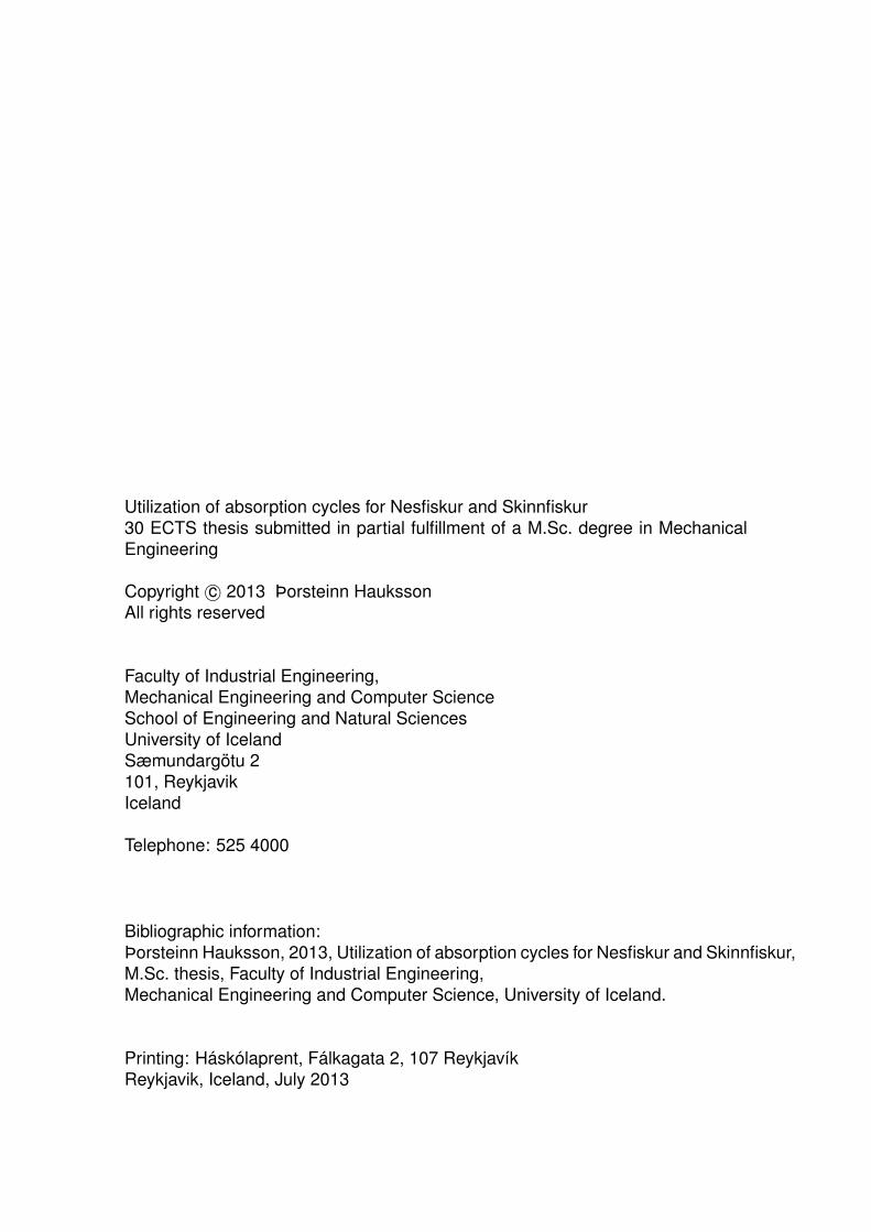
One way to calculate the COP for the compression cycle, is to estimate the energy absorbedfrom the fish in the freezer. To compute the energy loss in the fish, the enthalpy differencehas to be discovered and it depends on the initial and final temperature of the fish. Figure2.5 (Figure found in (Rha, 1975)) shows the enthalpy difference in a fish muscle.

8

Water proportion

84

11,1

Figure 2.5: Enthalpy difference in a fish muscle from 10− (−18)◦C.

The energy needed to freeze the fish is found from equations 2.3 and 2.4:

Q = m ·∆h (2.3)

h is found in figure 2.5 and ∆h is calculated from equation 2.4.

∆h = h0 − hend (2.4)

9

2.4. Methodology for the calculations in theproblem

This section addresses the calcualations for the flow inside pipes and the pressure dropper meter. The equations for the area of the heat exchangers are discussed and equationsrelated to the cost estimation.

The flow inside the pipe can be determined from equation 2.5:

G = Q

ρ ·∆h (2.5)

Where : G l/s FlowQ kW Power consumptionρ kg/dm3 Density∆h kJ/kg Enthalpy difference at inlet and outlet

The pressure drop per meter was calculated with following equations:

V = 4Qπd2

i

(2.6)

Re = V diυ

(2.7)

1√(f)

= −4.0log10

[ε/D

3, 7 + 1, 26Re√f

](2.8)

∆pf = fρL

D

V 2

2 (2.9)

The equations listed in 2.6 and 2.9 are found in (Crowe, 2005). The equation for friction(f ) is derived from the Colebrooks White equation and the pressure drop ∆pf is given bythe Darcy-Weisbach equation.

The area for each heat exchanger is calculated with following equation:

A = Q/(∆Tm × U) (2.10)

10

The Logarithmic-mean temperature difference (Tm) can be calculated for counterflowheat exchanger with equation 2.11:

∆Tm = ((T ′1 − T ′′2 )− (T ′2 − T ′′1 ))ln(T

′1−T

′′2

T ′2−T

′′1

)(2.11)

Where : T ′1 = Input temperature of the hot fluid[◦C]T ′2 = Output temperature of the hot fluid[◦C]T ′′1 = Input temperature of the cold fluid[◦C]T ′′2 = Output temperature of the cold fluid[◦C]

In this thesis the heat exchangers are assumed to be counterflow, where the colder fluidcan then reach a higher temperature than in cocurrent flow systems.

The cost of the equipment used in the absorption system can be calculated from equation2.12.

CPE,Y = CPE,W

(XY

XW

)α(2.12)

Where CPE,Y is the cost of an equipment item at a given capacity or size(XY ), CPE,Wis the purchase cost of the same item at a different capacity or size(XW ) and is a knownparameter. α is an exponent which is found in table 2.2 (A. Bejan, G. Tsatsaronis, 1996).

To calculate the profitability we find the present value of an annuity (PVOAA), which iscalculated from the present value (PV) of the annuity from the maintenance and electricitycost with addition to the initial cost (see equation 2.13) (Broverman, 1996).

Ct = Cc + Cei

(1− 1

1 + iT

)(2.13)

where : Ct = PVOAACc = Initial costCe = Annual costT = Expected life timei = Interest rate

The annual electricity cost is calculated with equation 2.14. The time t is counted inmonths and the interest rate (i) is 10 %.

11

Table 2.2: Determination of factor α

Equipment Variable X Size Range Exponentα

Pump (centrifugal;including motor) Power0.02−0.3 kW 0.23

0.3−20 kW 0.3720−200kW 0.48

Pump(vertical;including motor) Circulatingcapacity

0.06−20 m3/s 0.76

Evaporator SurfaceArea

10−1000 m2 0.54

Flat plate heat exchanger SurfaceArea

15−1500 m2 0.4

Shell & tube heat exchanger SurfaceArea

15−400 m2 0.4

Separator(centrifugal) Capacity 1.4− 7 m3 0.49

Ce =12∑t=1

Celect(1 + i)t/12 (2.14)

2.5. Absorption model

This section addresses the absorption cycles which are used in this thesis. The modelswhich the project is based on are single stage and two stage absorption cycles. The singlestage model is not as thermally efficient as the two stage model but the latter is morecomplex and requires a higher temperature of heat input. Additionally, the initial cost isgreater (Gregory Zdaniuk & Blackwell, 2012, p. 346). To solve each case an optimizationis made for chosen variables. The optimization method used is described in the end of thechapter.

2.5.1. Model of a single stage absorption cycle

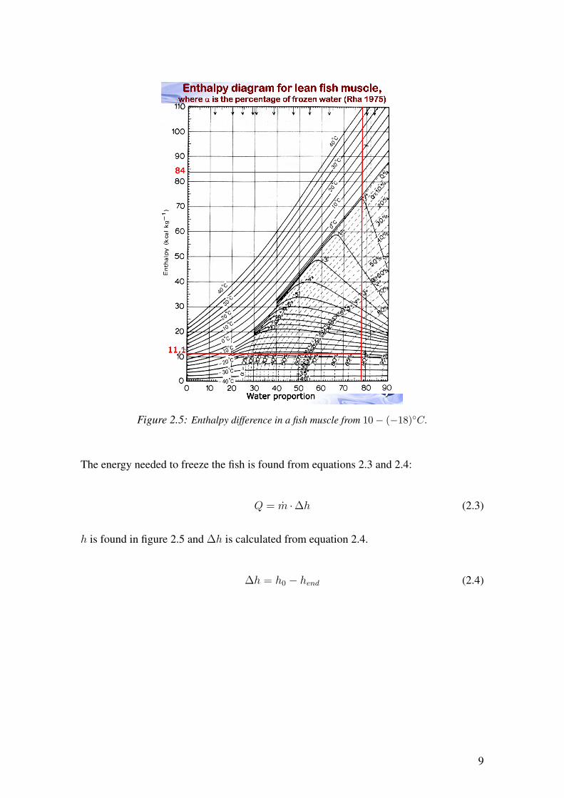
A single stage absorption cycle with water/ammonia solution as a working fluid consistsof a condenser, throttle valve, evaporator, absorber, rectifier, pump, generator and heatexchangers. In figure 2.6 a typical absorption cycle is shown (S.A. Adewusi, 2004,

12

p. 2358). The input and the output of the model are denoted by arrows, pointing to andaway from the component, respectively.

Figure 2.6: Absorption cycle

The function for each component in the cycle are as follows:

• Pump: The H2O/NH3 solution is pumped and the pressure increases. First theprocess is assumed to be isentropic. The ideal enthalpy (h2s) is calculated where theentropy remains constant and the higher pressure is given. Then the efficiency of thepump (ηp) is given and the nonisentropic enthalpy (h2) calculated from followingequation:

h2 = h1 + h2s − h1

ηp(2.15)

Eq. 2.16 models the work of the pump (Wp):

Wp = m1 · v1(P2 − P1)ηp

(2.16)

• Solution heat exchanger (SHX): The solution flows into a heat exchanger and heats

13

the solution with fluid from the generator. To find the heat difference in a heatexchanger the conservation of the energy is used, but it is described with followingequation:

m2(h3 − h2) = m15(h15 − h16) (2.17)

• Mixing fluids: When two fluids are mixed together, energy conservation is assumed:

m4h4 = m3h3 + m5h5 (2.18)

And the mass flow balance is:

m4 = m3 + m5 (2.19)

• Generator: An external source, heats up the solution in a heat exchanger, thus a partof the solution turns into vapor. Greater proportion of the vapor is ammonia, thereason being that the ammonia has a lower temperature for evaporation. The twophase flow separates in the separator and the liquid part flows into the SHX but thesteam continues to the rectifier. Mass flow of each phase in the separator is foundfrom the quality of the two phase flow after the heat exchanger as equations 2.20and 2.21 describe.

m7 =q6 · m6 (2.20)m15 =(1− q6) · m6 (2.21)

• Rectifier: The role of the rectifier is to distil the ammonia in the H2O/NH3 solutionfrom the generator. That is done by humidifying the vapor slightly, thus the solutionis hydrated. Surplus lean solution goes back to the circulation at point 5 in figure2.6. There are two rectifiers used, reflux coolers and distillation columns.(Ólafsson,Þ., 1999)

• Condenser: The condenser cools down the ammonia vapor with a heat exchangeprocess. Cold medium, flows into the condenser and condenses the vapor. Thus theammonia becomes liquid. This is a heat exchanger process.

• Throttle Valve: The pressure of the refrigerant is reduced significantly so the temperaturedecreases to the value which is maintained in the evaporator.

• Evaporator: Is a heat exchanger on the suction side of the absorption cycle. This

14

is where the ammonia evaporates for refrigeration. The ammonia vapor entersthe evaporator and the heat is transferred from the refrigerated space with a heatexchange process. If the system is designed to cool air directly, the evaporator isa air conditioner. If the role of the evaporator is to cool liquid, the refrigerant issprayed over tubes containing the fluid to be cooled. Typically tube and shell heatexchangers are used for such processes. Another kind of an evaporator is a platefreezer but they are common when freezing food products quickly.Where the ammonia has very low temperature at a low pressure, the designer has tochoose the right type of evaporator for it to function correctly in low pressure.

• Absorber: The evaporated refrigerant (ammonia) passes into the absorber whereit is mixed with an absorbent/refrigerant solution which has very low refrigerantcontent. This solution absorbs the vapor from the evaporator section.

Figure 2.7 (Figure taken from (Conde-Petit, 2004, p. 34)) shows an Othmer diagram(PTX) of H2O/NH3 solution. It describes the changes of temperature, pressure and theNH3 ratio after each component in a single stage absorption cycle which is shown infigure 2.6.

ABS AbsorberCND CondenserEVP EvaporatorGEN GeneratorRC Rectication ColumnRHX Refrigerant Heat ExchangerRRXV Refrigerant Expansion ValveSHX Solution Heat ExchangerSPP Solution Expansion ValveVR Reux Valve

Figure 2.7: Descriptive diagram of a H2O/NH3, single stage absorption system

In figure 2.7, denotes ξ the liquid phase of the solution and ζ denotes the vapor phase.

15

2.5.2. Optimization

The optimization method used for this project is called CMA-ES and stands for CovarianceMatrix Adaptation Evolution Strategy. CMA-ES searches for a minimal solution in acontinuous domain:

f : χ ⊆ Rn → R,x 7→ f(x) (2.22)

CMA-ES is an evolutionary algorithm for difficult non-linear non-convex optimizationproblems in a continuous domain. The advantage of the evolution strategy is that gradientcalculations are not necessary, only the object function values are needed, that means thatthe object function doesn’t need to be linear. The CMA-ES method samples a number ofnew candidate solutions from a multivariate normal distribution and then updates thesampling distribution exclusively using the better solutions. This method resembles theprinciple of biological evolution where some better individuals are selected for the nextgeneration.The update consists of two mechanisms, the step-size control where the length of the pathof the most recent iteration step are analyzed and the covariance matrix adaptation(CMA)which increases the likelihood of successful steps. This method has been used successfullyin real-world problems (Guillaume Collange, 2010).The reason for using an evolutionary algorithm for the optimization is that the functioninvolves iteration for solution properties which can give a discontinuous solution. Thereforethe gradient cannot be used.

16

3. Case studies and results

This chapter addresses the case studies and results. Among the issues discussed are thegeothermal provider, the energy available, the electricity cost, etc. The consumers whichare assumed to use the service are two companies in the fish industry, Nesfiskur andSkinnfiskur. The location of both companies is the Reykjanes peninsula (RP) in Iceland.

We will consider three cases of refrigeration system setups and calculate the profitabilityfor each to determine if they are feasible. In the cases we use modified models of thesingle stage and two stage absorption systems that were mentioned in chapter 2. All themodel codes are written in the python programming language, the optimizations weredone with CMA-ES code (see section 2.5.2) and the drawings are generated in AutoCad.

3.1. HS veitur

HS veitur is one of the largest energy companies in Iceland and over the years the companyhas supplied and distributed hot water, fresh water, electricity and dispose sewage inseveral areas in RP and Vestmanneyjar. The energy source for the hot water and theelectricity comes from a geothermal source, since RP is located in a high temperaturegeothermal area. The idea is to use one of the geothermal sources to produce refrigerationwith absorption technology for companies nearby that consume large amounts of electricenergy for refrigeration systems.The plant studied in this thesis is a single flash geothermal power plant and is located inReykjanes, Reykjanes Power Plant (RPP). The reason for studying this plant is that someamount of hot water is not used and discarded into the sea. The temperature of the wastewater is 211 ◦C and the mass flow is 200 kg/s. The geothermal energy that is unused ishigh and there is a potential to utilize that energy. [Geir Þórólfsson Engineer at HS veitur(2012)].The price for electricity for the general public utilities is 5.18 kr/kWh but for large powerconsumers (> 3000 kWh/yr) the price drops down to 3.5 kr/kWh [Jóhann Sigurbergssonat HS-veitur (2012)].

17

3.2. Description of the companies involved

There are few a companies, mainly in the fish industry in RP that consume enoughelectricity for freezing to be interesting case studies for whether it’s profitable to changerefrigeration systems. Two companies are studied in this thesis, Nesfiskur ehf and Skinnfiskurehf. They use compressors as described in section 2.1 which uses more electricity thanabsorption cycles. We will consider whether absorption systems are cheaper and a moreconvenient choice.

3.2.1. Nesfiskur ehf

Nesfiskur ehf is a large fishery located in Garður, RP. The distance between Nesfiskur andRPP is approximately 30.5 km.Nesfiskur uses two kinds of freezers. One is a deep freezer where the temperature reachesa very low value, about−40 ◦C and freezes the product in a short time. The second freezeris used to store the fish at low temperature which is about−24 ◦C to−25 ◦C but consumesonly 18 kW so we will not consider it.The usage of the deep freezer varies from day to day and depends on when the trawlerscome ashore with the fish. When a trawler has delivered fish, it is prepared on conveyorsand part goes into the deep freezer while the rest goes directly to sale. The temperatureinside the deep freezer in October 2012 is shown in figure 3.1. [Friðbjörn Júlíusson atNesfiskur(2012)].

Oct 14 2012

Oct 16 2012

Oct 18 2012

Oct 20 2012

Oct 22 2012

Oct 24 2012

50

40

30

20

10

0

10

20

30

Tem

pera

ture

[◦C

]

Temperature range in a freezer in Nesfiskur for few days in October

Figure 3.1: Temperature range in a deep freezer at Nesfiskur ehf.

The temperature in the evaporator varies from −40 ◦C to −35 ◦C until the freezing isfinished. The time span of the freezing varies but from figure 3.1 it can be detected thatthe duration of one period is approximately 12 hours.

The medium to condense the refrigerant is seawater. The seawater is 7 ◦C throughoutthe year [Friðbjörn Júlíusson at Nesfiskur(2012)]. A lot of electricity is used to maintainthe low temperature in the freezer at a high refrigeration power output. The COP ofthe compression cycles varies from 1.44 to 2.01. The current use is 950 A and the electric

18

power consumption goes up to 890 kW when everything is running. The total refrigerationpower output is ≈ 1700 kW. See figure 3.2

Nov 2011

Dec 2011

Jan 2012

Feb 2012

Mar 2012

Apr 2012

May 2012

Jun 2012

Jul 2012

Aug 2012

Sep 2012

Oct 2012

0

200

400

600

800

1000

1200

Pow

er[kW

]

Electricity range in Nesfiskur over a year

Sep 27 2012

Oct 04 2012

Oct 11 2012

Oct 18 2012

0

200

400

600

800

1000

1200

Pow

er[kW

]

Electricity range in Nesfiskur from 24/9/12 to 24/10/12

Figure 3.2: Power usage in Nesfiskur for different time periods.

The majority of energy consumed is used by the compressor but other usage includesconveyors, refrigerators and other equipment. Figure 3.2 depicts that spikes increasesfrom October 2011 to October 2012 which means that freeze use increased in that year.In the calculations, late September and October 2012 are considered since those monthsincluded the most recent data at the time of writing. To calculate the electricity usage forthe compression part, the electrical power spikes in figure 3.2 are integrated over timeinterval (in hours) and the other activity is subtracted from the integration, see equation3.1.

I =tend∑t0=0

(P (t)Compressors − POther) (3.1)

In eq. 3.1 I is electricity consumption in kWh, t0 and tend define the time span and POtheris approximated as 150 kW. The power consumption for the compressors from sept. tookt. is 227.000 kWh, the electricity cost for the freeze is listed in table 3.11

1Electricity price list obtained from HS-Orka and HS-Veita

19

Table 3.1: Electricity cost at NesfiskurHS-Orka Used Elect.(kWh) Price rate(kr/kWh) Price(kr)Energy tax 227, 240.90 0, 12 27, 268.9Energy rate 227, 240.90 3.51 797, 615.625, 5% VAT 210, 345.5

Total 1,035,230HS-Veita

Distribution price 227, 240.90 1.98 449, 937Transportation price 227, 240.90 0, 83 188, 609.9

25, 5% VAT 162,829.5Total 801, 376.4Total 1,836,606

More detailed information about the freezers can be found in table 3.2.

Table 3.2: Power used by the freezers in Nesfiskur.Type Evap. temp.(◦C) Power in.(kWh) Evap. out.(kW) COP

Blast freezer 1 −40 260 375Blast freezer 2 −40 310.13 511.72

Screw Compressor 1 −35 214 387Screw Compressor 2 −40 167 336

freezers 3x −40 60 86.4 1.44Total 1011.13 1696.1 1.67

Table 3.3: Other refrigeration systems that are not taken into consideration but could bereplaced with an absorption system.

Type Evap. temp.(◦C) Power in.(kW)

Raw food cooler 2 18Storage freezer −22 25Bacalao cooler 5 15

Fillet cooler 2 15Total 133

The unit for capital in the calculation is Million Icelandic krona(MISK). The annual costfor maintaining the compression system is 2.4 (MISK) [Friðbjörn Júlíusson at Nesfiskur].

3.2.2. Skinnfiskur ehf

Skinnfiskur ehf is located in Sandgerði which is about 27.4 km from RPP. Their product isfrozen fish offal for animal consumption for external and internal markets. To freeze their

20

product they use similar technology as Nesfiskur. The freezer has two steps, lower stepcompression and higher step compression. The lower step runs on lower temperature,around −3 ◦C to −8 ◦C but for the higher step the temperature ranges from −32 ◦C to−37 ◦C on the suction side of the compressor. Table 3.4 shows data for compressorsrunning at the date Nov 11. 2012, describing a typical day at Skinnfiskur.The temperature drops from the evaporator to the compressor due to pressure difference.The ideal temperature to be contained in the evaporator is−40 ◦C [Sigurður Jónas Bergssontechnologist at Frosti hf].

Table 3.4: Power use of the compressors at Skinnfiskur.Type Compressor Temp.(suction side)(◦C) Power in(kW)

High step compressor 1 −37 142.7High step compressor 2 −32 150.34Low step compressor 1 −5.8 119.9Low step compressor 2 −3.5 122.6

Total 535.54

Table 3.5 shows how one compressor would function instead of all four compressors, thisis done to simplify the calculations.

Table 3.5: Ideal CompressorType Evaporator Temp.(◦C) Power in(kW) Evap. out.(kW) COP

Ideal compressor −40 535.54 1017.53 1.9

It is hard to determine the COP for the system but it is approximated to be 1.9 for eachcompressor assembly [Sigurður Bergsson at Frosti].The freezer is a plate freezer but the fish is planted in trays and placed in the freezer. Nextthe fish is cooled from 10 ◦C to −18 ◦C. The freezer can ingest about 13.3 tons at a time,and the duration of each replacement is 100 min. [Skúli Guðmundsson at Skinnfiskurehf].If the COP is calculated from the fish muscle, which is descriped in section 2.3 from thegiven condition, the real COP of the present system should be 1.264. Here we assumethat all the refrigerating energy goes directly into the fish with no losses of energy out ofthe system. However in reality the energy loss in the freezer is unavoidable.The electricity cost for October 2012 is 1.057 MISK for electric power consumption and0.933 MISK for the electric distribution fee. A total of 1.990 MISK [Electric cost atSkinnfiskur for October 2012].By using a two step compression systems the efficiency increases at the expense of capitalcost. The electricity cost at Skinnfiskur varies from month to month but depends on howmuch of the material is imported from other fisheries.The annual cost for maintaining the compression system is 1.6 MISK [Bárður Bragasonat Skinnfiskur]

21

3.3. Case A - Pipeline from Reykjanes toSkinnfiskur and Nesfiskur

In case A we consider hot water from a geothermal source to heat the working fluid in anabsorption cycle, the geothermal source being RPP. The main expense comes from pipeconstruction for transporting the geothermal water, where it is used in an absorption cycle.A problem can occur if the water from the geothermal borehole is transferred over longdistances. Silica particles can form scaling along the way when the temperature of theliquid decreases. Therefore a groundwater source is used as a mediate and heated up in aheat exchanger and then sent to the refrigeration plant. Suggestion to changes on RPP isshown in figure 3.3

Figure 3.3: Reykjanes power plant after possible changes

22

The mass flow at point 16 in figure 3.3 is 244 kg/s (Benediktsson, D. Ö., 2010, p. 8) at211 ◦C with pressure at 19, 8 bar (Jóhannesson, Þ., 2011).

The surplus water in RPP would be transported through pipelines specially constructedfor this project. The distance is quite long, from Reykjanes to Sandgerði and Garður asshown in figure 3.4. In the scenario, the water to Skinnfiskur and Nesfiskur has a sharedpipeline, large part of the route. This means they can share expenses for the pipeline.Skinnfiskur would pay weighted proportion of the fee for the first 26, 3 km of pipelinealong with Nesfiskur and then pay the last 2, 0 km exclusively while Nesfiskur wouldpay for 6, 0 km of the pipeline for themselves. The cost of the pipeline depends on thediameter of the pipe, which can be determined from the water consumption.

Figure 3.4: Pipeline from RPP to Skinnfiskur and Nesfiskur [Map taken from www.ja.is].

3.3.1. Nesfiskur

In this section we address how the absorption system for Nesfiskur would function forcase A. We determine the flow from RPP, choice of heat exchangers, pressure drop in thepipelines from RPP and more related.

To compute the mass flow and temperature required for the absorption cycle, we haveto optimize and modify the single stage model which is shown in figure 2.6. After themodification the SHX and CEHX are removed from the model. Modified model for thiscase is shown in figure 3.5

23

Figure 3.5: Modified single stage absorption cycle for case A

Since the thermal energy of the source water from RPP is very high we can remove SHXand CEHX from figure 2.6 and utilize the source in the desorber. This lowers the COP butit does not affect the power output of the evaporator. This is done to lower the expense ofthe model.

24

Optimizing the mass flow is a problem with several constraints:

• Mass flow of water from RPP can be up to 200 kg/s and the temperature can bemaximum 206 ◦C at 18, 6bara.

• Steam from the rectifier is almost pure ammonia thus the evaporator can run on lowtemperature.

• The coolant in the condenser is the seawater which has the temperature 7 ◦C, whichmeans that it can’t cool lower than 12 ◦C since it is assumed that the pitch in theheat exchanger is 5 ◦C.

• Heat output from the evaporator is approximated 1700 kW at temperature of−40 ◦C

• The mass flow must be conserved and be equal at points 15 and 1 in figure 3.5.

• The fluid from the absorber must be in liquid phase and the temperature above12 ◦C.

• Temperature of the water in the pipelines from RPP can reach up to 160 ◦C but thatis the design temperature for the pipelines from SET (Set, 2012).

The optimization involves minimizing the mass flow from RPP provided that the evaporatorheat output should be 1700 kW. the mass flow is minimized for the provided evaporatoroutput. Next the constraints for certain variables are created within reasonable limits.Now the mass flow from Reykjanes power plant is optimized with respect to:

1. The high pressure that the pump produces (phigh)

2. NH3 : H2O ratio at point 1

3. Mass flow of the working fluid at point 1 (m1)

4. Temperature of the working fluid at the desorber output (T6)

Results from the optimization are shown in table 3.6.

Table 3.6: Optimization for the mass flow from RPP, case A - Nesfiskur

m1[kg/s] phigh[kPa] x[NH3,H2O] T6[◦C] m16[kg/s] Qevap[kW] COP

11.98 700.47 [0.3393, 0.6607] 99.87 13.384 1700.0 0.252

The COP for the optimization is 0.626 which would generally not be considered efficient.The power of the circulation pump in the cycle is 9.44 kW with 90 % efficiency. There isa clear interaction in the optimization between the NH3 : H2O ratio and the high pressure.Fig. 3.6 depicts how the power in the evaporator changes with aforementioned variables.

25

Figure 3.6: How evaporation power depends on pressure and the NH3 : H2O ratio.

Results for the properties at each point in the diagram (fig. 3.5) is found in section A.1under Appendix A.

That is because the cost of the pipe depends on the pipe diameter. The temperature ofthe water should also be considered where the temperature tolerance limit of the pipeis restrictive and the lifetime of the pipe decreases with higher temperature where theisolation of the pipe has limited tolerance. The temperature of the district heating pipespurchased from Set hf are designed for a maximum at 160 ◦C. If the temperature is higheranother type of pipe has to be chosen and the pipe cost will increase significantly [ÖrnEinarsson, Engineer at Set hf (2012)].The neccesary flow in the the pipes from Reykjanes can be calculated from equation 2.5:

Where : G = 14.745 l/sQ = 6, 791.0 kWρ = 0.9077 kg/dm3

∆h = 675.8− 168.3 kJ/kg

Available pipe diameters are given at Set hf with the cost per meter (Set, 2012). ThePressure drop (∆pf ) and the velocity (V ) of the flow is calculated in table 3.7 for thedesign.

Table 3.7: Flow in different pipe diameters

di[mm] Q[m3/s] V[m/s] Re f ∆pf [Pa/m] Cp[kr/m]125 0.014745 1.202 799, 941 0.0123 64.21 5080150 0.014745 0.8344 666, 617 0.0126 26.55 6300200 0.014745 0.469 499, 963 0.0132 6.61 9580

The pressure drop per meter was calculated with equations from 2.6 to 2.9. In the standards

26

in (Set, 2012) it’s recommended that the pressure drop does not exceeds 100 Pa/m,therefore the 125 mm pipe should be chosen for Nesfiskur.

Choosing the right heat exchanger can be difficult. There are many types available butthose who are mostly used are plate and shell & tube heat exchangers. Low cost is veryimportant in the design and the shell and tube type are rather chosen where the plate heatexchangers are more expensive.

Table 3.8 lists all the detailed information for each heat exchanger.

Table 3.8: Overall heat coefficient, area and energy consumption for heat exchangers -Case A, Nesfiskur

Comp.\Var. Type U[kW/m2K] Q[kW] A[m2]

Desorber Shell&Tube 0.71 6791.0 934.4Rectifier Shell&Tube 0.71 1141.5 31.3Condenser Shell&Tube 0.71 1973.3 479.3Evaporator Plate freezers 1.65 1700.1 32.1Absorber Shell&Tube 0.71 6530.3 1783.8

Value for U can vary, it’s related to the individual film heat transfer coefficients, foulingand wall resistances, massflow and the outside surface area. U in table 3.8 is calculatedfrom U values are for Evaporator found in (Granryd, 2009), other U values found in(Spang, 2012)). The evaporator is assumed to be a plate freezer which are designed toquick freeze food products like fish. The evaporator is not taken into account in the costestimation since it is possible to use the existing one at Nesfiskur.

The temperature profiles for each heat exchanger can be found in figure A.1. The constraintsfor counterflow heat exchangers is that the temperature of each liquid can not cross thepitch which we use as 5 ◦C. The pitch is the minimum temperature difference betweenthe fluids. In figure 3.7(a) and 3.7(b) we observe that the lines are parallel at 5 ◦C distancefrom each other which means that the model is successfully optimized.

27

0 1000 2000 3000 4000 5000 6000 7000Energy(Q[kJ])

20

40

60

80

100

120

140

160Tem

pera

ture

(T[◦C

])Desorber

(a)

0 1000 2000 3000 4000 5000 6000 7000Energy(Q[kJ])

5

10

15

20

25

30

35

40

45

Tem

pera

ture

(T[◦C

])

Absorber

(b)

Figure 3.7: Heat exchange process for the desorber and absorber

3.3.2. Skinnfiskur

In this section we address the calculations for Skinnfiskur. The methodology is the sameas in section 3.3.1, but the conditions are not the same. The model is the same but theevaporation power output is less.

For Skinnfiskur the optimization conditions change. The Evaporator output is now 1020 kW.The optimization is executed in CMA-ES for high pressure (phigh), NH3 : H2O ratio andthe mass flow of the working fluid at point 1 and T6 (see figure 3.5). Results for thisoptimization is shown in table 3.9

Table 3.9: Optimization for the mass flow from RPP - case A, Skinnfiskur

m1[kg/s] phigh[kPa] x[NH3,H2O] T6[◦C] m16[kg/s] Qevap[kW] COP

9.00 700.0 [0.34, 0.66] 94.84 8.46 1020 0.222

Properties for each point in the cycle along with the temperature profile for each heatexchanger can be found in section A.2 under the Appendix A. The COP of the cycle is0.222 which is similar to the COP at Nesfiskur and the work of the circulation pump is7.1 kW.

28

To determine the pipeline diameter, the pressure drop per meter is found from equations2.5, 2.6, 2.9, 2.8 and 2.7. Results are shown in table 3.10

Table 3.10: Flow in different pipe diameters - Skinnfiskur

di[mm] Q[m3/s] Vm/s Re f ∆pf [Pa/m] Cp[kr/m]125 0.00932 0.759 505.626 0.01325 27.73 5080150 0.00932 0.527 421.355 0.0137 11.49 6300200 0.00932 0.297 316.016 0.01438 2.87 9580

The most sensible choice for Skinnfiskur is the 125 mm diameter, It’s cheapest and thepressure drop is within limits.

The result for heat exchanger characteristic is shown in table 3.11. The methodology isthe same here as in section 3.3.1.

Table 3.11: Overall heat coefficient, area and energy consumption of heat exchangers -Case A, Skinnfiskur

Comp.\Var. Type U[kW/m2K] Q[kW] A[m2]

Desorber Shell&Tube 0.71 4597.7 455.4Rectifier Shell&Tube 0.71 524.7 14.1Condenser Shell&Tube 0.71 1184.1 266.0Evaporator Plate freezer 1.65 1020.0 19.23Absorber Shell&Tube 0.71 4442.4 1228.3

29

The pipeline is a little longer than the 26,3 km straight line from RPP to the pipe junctionshown in fig. 3.4. A few more kilometers are added due to extra loops on the way toreduce the thermal expansion and also because the pipeline is not in straight line due tolandscape. This doesn’t affect the calculation much. The diameter for the pipe is foundout with the flow from Skinnfiskur and Nesfiskur which is m = 24.065 dm3/s. Now wededuce the diameter like before (see table 3.12).

Table 3.12: Pipe diameters - Skinnfiskur and Nesfiskur

di[mm Q[m3/s] V [m/s] Re f ∆pf [Pa/m] Cp[kr/m]125 0.024065 1.961 1, 305, 566 0.0113 158, 2 5080150 0.024065 1.362 1, 087, 972 0.0116 65.2 6300200 0.024065 0.7660 8, 159, 79 0.0121 16.2 9580250 0.024065 0.4902 652, 783 0.0126 5.4 14, 085

In table 3.12 the cost per meter is quite high, the diameter ranges from 150 mm to 200 mm,the economical choice being 150 mm. The pressure drop is within limits. The table onlyshows the flow if both systems are running at the same time at Nesfiskur and Skinnfiskur.Storage tank near the pipeline junction would work as a buffer so the flow from RPPdoesn’t need to be as much and can be controlled in a better manner. Then the watercould be dispensed to the companies when required. The benefits from this is that thepressure drop in the pipelines decreases.

The pressure drop due to the length of the pipe is:

∆pNes,Skinn = 1, 714.8 kPa (3.2)

The pressure drop from the separation of pipeline to Nesfiskur is ∆pNes = 385.26 kPaand to Skinnfiskur ∆pSkinn = 55.46 kPa. This means that the pump or pumps have toincrease the pressure up to 4475 kPa to reach 1100 kPa at the end.

30

3.3.3. Cost estimation

In this section we address the cost for each case and examine whether it’s feasible for thecompanies to choose one of the cases.It is assumed that both companies will agree choosing the same case, the cost is dividedwhere there is need to determine the cost for the pipes and the pumps.

The cost analysis for case A divides into two parts, initial cost and annual cost. The initialcost factors for the setup of the system are:

• The pumps: Borehole pump to supply ground water which is heated up in RPP.Stage pump to increase the pressure from RPP to Garður and Sandgerði and acirculation pump that is used in the cycle.

• The pipelines: Pipeline from RPP to Garður and Sandgerði.

• Heat exchangers: In the absorption cycle

• Construction cost

• Other devices: Expansion valves, control valve, electrical control & monitor system.

• Civil structural and architectural work

• Design and supervision

Annual cost is low for this project, since the system mainly has mechanical componentswhich rarely fail, but the cost can increase if the electricity usage for the pumps becomesan issue, mainly the stage pumps.

The weighted cost ratio between Nesfiskur and Skinnfiskur depends on the mass flowneeded for each company. The share ratio for Nesfiskur is 0.6127, calculated from massflow(m16) in tables 3.6 and 3.9. The pipe is the largest cost factor. The total piping costfor Nesfiskur is Cp,n = 132 MISK. Equation 2.12 is used to calculate the cost of theequipment used in the absorption system.

Cost analysis for heat exchangers and pumps are listed in table 3.13

31

Table 3.13: Estimate cost for components in case A - Nesfiskur

Comp.\Var. CPE,W[MISK] XW XY α CPE,Y[MISK] Total[MISK]

Borehole pump 1.01 31.9 kW 19.9 kW 0.48 0.806 0.49Stage pump 2.080 40.3 kW 123.0 kW 0.48 3.554 2.18Circulation pump 0.890 18.93 kW 9.4 kW 0.37 0.688 0.69

Pumps total 3.36

Desorber 111.104 850 m2 934.4 m2 0.4 115.39 115.39Rectifier 111.104 850 m2 31.3 m2 0.4 29.661 29.66Absorber 111.104 850 m2 1783.8 m2 0.4 149.452 149.45

Hx.Total - Hx 294.5

The Stage pump and the borehole pump are located in RPP and are bought for Nesfiskurand Skinnfiskur which divide the cost. The condenser and evaporator are already in useat Nesfiskur and they can be used in this case as well.It is assumed that the expansion valves, control valve, electrical control & monitor systemcost 5 % of the pump and heat exchangers, which is 14.8 MISK. The source for the costof the heat exchanger wished to remain undisclosed.

The cost analysis for Skinnfiskur is calculated in the same manner as for Nesfiskur.The pipe cost for Skinnfiskur is 74.3 MISK. The costs for pumps and heat exchangers arelisted in table 3.14, the reference price is the same as in table 3.13.

Table 3.14: Estimate cost for components in case A - Skinnfiskur

Comp.\Var. XY Total[MISK]

Borehole pump 19.9 kW 0.31Stage pump 123 kW 1.38Circulation pump 123 kW 0.62

Total - Pumps 2.31

Desorber 455.4 m2 86.56Rectifier 14.1 m2 21.56Absorber 1228.3 m2 128.73

Total - Hx 236.85

The cost for expansion valves, control valve, electrical control & monitor system is11.87 MISK

32

If the companies agree on choosing case A a rough estimation on the investment costwould be as listed in table 3.15 (Ólafsson, Þ., 1999, p. 55).

Table 3.15: Breakdown of total capital investment, Case A

Direct Cost (DC) Nesfiskur Skinnfiskur

Onsite cost (ONSC) (MISK) (MISK)

Pipes 132.0 74.3pumps 3.4 2.3Heat Exchangers 295.5 236.9Electrical control&monitor system 14.8 11.9

Total ONSC 445.7 325.4

Offsite cost (OFSC)Civil, structural andarchitectural work 15%of ONSC

66.8 48.8

Total DC 512.5 374.2

Indirect Cost (IDC)

Engineering andSupervision (10% ofDC)

51.3 37.4

Construction cost (15%of DC) 76.9 56.1

Total IDC 128.2 93.5

Total CapitalInvestment (TCI) 640.6 467.7

The investment cost is very high compared to the other cases and it is likely that table3.15 is an underestimation as the cost will increase due to components and other chargesthat are not mentioned.

The annual cost is the annual maintenance cost(Cm) of the absorption system and theelectricity cost (Celect) of the pumps. The usage from the freezers are approximately 70%per month(seen from figure 3.2) and the electricity price per kWh is calculated with thereference to table 3.1. To calculate the annual electricity cost equation 2.14 is used andPVOAA is calculated from equation 2.13.

For the present value of an PVOAA, the time span is 30 years with the interest rate of10 %. In table 3.16 the unchanged compressor system (UC) is compared to case A (CA)version.

33

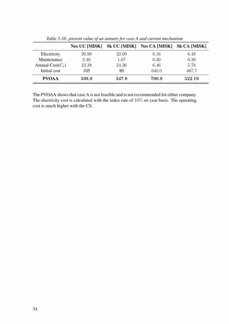
Table 3.16: present value of an annuity for case A and current mechanism

Nes UC [MISK] Sk UC [MISK] Nes CA [MISK] Sk CA [MISK]

Electricity 20.98 22.69 6.16 6.48Maintenance 2.40 1.67 0.30 0.30

Annual Cost(Ce) 23.38 24.36 6.46 5.78Initial cost 105 80 640.0 467.7PVOAA 338.0 347.8 700.9 522.19

The PVOAA shows that case A is not feasible and is not recommended for either company.The electricity cost is calculated with the index rate of 10% on year basis. The operatingcost is much higher with the CS.

34

3.4. Case B - Use of a district heating system

Another approach is evaluated to find an economical solution for Nesfiskur and Skinnfiskur.That is to use the district heating system from HS-veitur. The capacity of the districtheating system at Vellir in Keflavik is approximately 150 l/s in addition to the hot waterthat is in use and the temperature of the water is 90 ◦C. It’s possible to use this heat inan absorption cycle and return the water into the district heating system at a temperatureabove 70 ◦C, which is the normal temperature of the hot water for general use (See figure3.8).

Figure 3.8: Modified District heating system

The map of the pipeline from Vellir is shown in figure 3.9 (Map is taken from www.map.is).

Figure 3.9: Pipeline from Vellir to Skinnfiskur and Nesfiskur

Case B addresses the optimization for the absorption cycle with challenging constraintswhere the temperature of the source is low and the flow is limited. We will consider

35

whether the system is feasible with the limited flow.The problem changes, now the efficiency is more important and it is necessary to use heatexchangers to increase the COP.

Figure 3.10: Modified single stage absorption cycle for case B

The following constraints for case B are different from case A.

• The temperature from the source is 90 ◦C

• The source water out of the desorber must be above 70 ◦C

• The maximum flow from HS-veitur is 150 l/s

• Evaporator output must be above 1700 kW and maintain −40 ◦C temperature.

Other relevant constraints are listed in section 3.3.1When case B was optimized the constraint for higher pressure was lowered to 658 kPa but

36

it can’t be any lower, since the condenser should be capable of liquidizing the refrigerant.The consequences of having lower pressure is that the flow of the coolant in the condenserwill increase significantly which means we require more power for pumping seawater intothe condenser.The task is well constrained and there are not many variables to optimize. The NH3 ratioat point 10 is set to 99, 6 % to allow the higher pressure to go lower. The purpose of havinglower pressure is to allow the solution to have a greater evaporation at 85 ◦C which is themaximum heating. NH3 ratio at point 1 is 34 %.

37

3.4.1. Nesfiskur

We deduce the right mass flow of the working fluid and present the results in table 3.17for the optimization.

Table 3.17: Optimization for the mass flow from the district heating system - Case B,Nesfiskur

m1[kg/s] m20[kg/s] QEvap[kW] COP

26.923 103.19 1700 0.343

The mass flow of the working fluid has increased from case A but that’s to be expectedas only 6, 4 % of the solution evaporates after the generation compared to 16 % in case A.The values for each point are found in section A.3. The work of the circulation pump is19.77 kW. The COP is surprisingly high considering the low generation temperature.The results for the heat exchangers are shown in table 3.18 and the properties of theworking fluid at each point and the temperature profiles in the heat exchangers are foundin section A.3 in Appendix A.

Table 3.18: Area and energy consumption of the heat exchangers in - Case B, Nesfiskur

Comp.\Var. Type Q[kW] A[m2]

SHX Shell&Tube 6020.6 184.2Desorber Shell&Tube 4929.6 1263.8Rectifier Shell&Tube 572.5 16.1Condenser Shell&Tube 2005.8 569.2CEHX Shell&Tube 101.3 25.1Evaporator Plate freezer 1700.1 30.6Absorber Shell&Tube 4644.0 1272.2

38

3.4.2. Skinnfiskur

The same calculation is performed for Skinnfiskur but the refrigeration power in theevaporator is now 1020 kW .

Table 3.19: Optimization for the mass flow from the district heating system - Case B,Skinnfiskur

m1[kg/s] m20[kg/s] QEvap[kW] COP

16.28 61.91 1020 0.343

The result shows that if both systems are running continuously, the district system cannotsustain the demand where the total flow would be 165.1 kg/s to Skinnfiskur and Nesfiskur.The properties of the heat exchangers are found in table 3.20. The work of the circulationpump is 11.9 kW. Other results can be found in section A.4.

Table 3.20: Area and energy consumption of the heat exchangers at - Case B, Skinnfiskur


SHX Shell&Tube 3612.2 110.5Desorber Shell&Tube 2957.6 758.4Rectifier Shell&Tube 343.5 9.7Condenser Shell&Tube 1203.4 321.0CEHX Shell&Tube 60.8 15.0Evaporator Plate freezer 1020.0 18.4Absorber Shell&Tube 2786.3 763.3

3.4.3. Piping system and pressure drop

The pipeline is connected to the pipeline in Vellir (see figure 3.9) from where the water istransported to its destination point. The pipe is divided in to three parts:

• Shared part, where the mass flow is 165.1 kg/s and should provide hot water forboth Nesfiskur and Skinnfiskur.

• Pipeline to Nesfiskur, the joint pipeline splits into two parts. The mass flow toNesfiskur is 103.2 kg/s.

• Pipeline to Skinnfiskur, the mass flow to Skinnfiskur is 61.9 kg/s.

The calculations in table 3.21 are based on equations that are described in section 3.3.1.

39

Table 3.21: Chosen pipe diameters in case B

Element.\Variable L[m] m[kg/s] ∆pf [Pa/m] pf [kPa] di[mm] CP[kr/m]Pipe(shared) 8300 165.1 89.7 744.5 300 20, 282Pipe(Nesfiskur) 5200 103.2 91.2 474.2 250 14, 085Pipe(Skinnfiskur) 3000 61.9 104.8 314.4 200 9, 580

A stage pump is used to maintain the pressure, located in Vellir and needs to increase thepressure difference to 1218.7 kPa which means that the power consumption of the pumpis 231.3 kW.

40


The methodology in this section is similar to the method used in section 3.3.3. First thecost analysis for each component is examined for both companies then the total capitalinvestment is determined and listed in a table and finally the present value of an annuityfor each company is determined.

The weighted share ratio for Nesfiskur and Skinnfiskur is [0, 625 : 0, 375]. It’s determinedfrom the mass flow(m20) in tables 3.17 and 3.19.The cost of the pipeline from Vellir to the companies can be calculated from the valuesin table 3.21. The cost analysis for components needed by Nesfiskur and Skinnfiskur arelisted in table 3.22. The price is calculated in equation 2.12 and the reference prices forcomponents are listed in table 3.13.

Table 3.22: Estimate cost for components - Case B

Comp.\Var. XY,Nes Total[MISK] XY,Skinn Total[MISK]

Stage pump 231.3 kW 3.0 231.3 kW 1.8Circulation pump 19.8 kW 0.9 11.9 kW 0.7Total - Pumps 3.9 2.5

SHX 184.2 m2 60.2 110.5 m2 49.1Desorber 1263.8 m2 130.1 758.4 m2 106.1Rectifier 16.1 m2 22.7 9.7 m2 18.5CEHX 25.1 m2 27.1 15.0 m2 22.1Absorber 1272.2 m2 130.4 763.3 m2 106.3Total Hx 3024.5 m2 370.6 1920.0 m2 302.1

Pipe(Shared) 8300 m 105.2 8300 m 63.1Pipe 5200 m 73.2 3000 m 28.7Total - pipes 178.4 91.8

Expansion valves,control valve, electricalcontrol & monitorsystem

5 % 16.69 13.6

41

The total capital investment for case B is listed in table 3.23. Where it is summarizedcosts for all components involved and scheduled potential cost of the project

Table 3.23: Breakdown of total capital investment, Case B

Direct Cost (DC) Nesfiskur Skinnfiskur

Onsite cost (ONSC) (MISK) (MISK)

Pipes 178.4 91.8Pumps 3.9 2.5Heat Exchangers 370.6 302.1Electrical control&monitor system 16.7 13.6

Total ONSC 569.6 410.0

Offsite cost(OFSC)Civil, structural andarchitectural work 15%of ONSC

85.4 61.5

Total DC 655.0 410.0

Indirect Cost (IDC)


65.5 47.2

Construction cost (15%of DC) 98.3 70.7

Total IDC 136.2 117.9

Total CapitalInvestment (TCI) 818.8 589.4

42

Next we calculate the PVOAA for each company with equation 2.13. The cost for theelectricity is mainly because of the stage pump located at Vellir. The flow needed is alotand the pressure drop in the pipes high. The cost for the equipment is quite high and theheat exchangers are expensive. The calculations are found in table 3.24

Table 3.24: PVOAA for case B and current mechanism

Nesfiskur[MISK] Skinnfiskur[MISK]

Electricity(Celect) 9.61 5.77Maintenance(Cm) 0.30 0.3Annual Cost(Ce) 9.91 6.07Initial Cost(Cc) 818.8 589.4

PVOAA 912.24 646.61

As seen in table 3.24 the cost is far above the limit and thus case B is not recommended.

3.5. Case C - Freezing plant

In case C a refrigeration system and warehouse is assumed to be built and located nextto RPP. The waste water from the plant is used as a heating source for the working fluid.Nesfiskur and Skinnfiskur could therefore transport their products to the warehouse forstorage. The temperature of the waste water is quite high, 211 ◦C. This high temperaturecan be used to improve the efficiency of the cycle by using two stage absorption systemswith two pressure levels. Seawater is assumed to be 9◦C in Reykjanes, which means thatthe temperature of the cooling in the condenser and absorber is 2◦C higher than in theother cases.

3.5.1. Model and optimization

The model which is modified from the model in figure 2.4, is shown in figure 3.11.

43

Figure 3.11: Modified of a two stage absorption cycle

The model has become more complex and has many factors that need to be consideredfor the simulation to function correctly. The constraints are the same as in section 3.3.1but now the temperature for the coolant in the condenser and absorber is 9 ◦C. The COPis maximized in the calculation and the optimization variables are:

1. NH3 : H2O ratio at point 1, the bounds are: [0.29; 0.71]:[0.326; 0.674].

2. Temperature after the generation of Generator I at point 6, the bounds are: [140; 206]◦C.

3. NH3 : H2O ratio for the steam to the condenser at point 10 and 19, the bounds are:[0.99; 0.01]:[0.99999; 0.00001].

4. Temperature for the output on SHX I at point 21, the bounds are [5; 35]◦C additionto the temperature of point 3.

5. The higher pressure (ph1) for generator I had the bounds [1700; 2800]

6. The lower pressure (ph2) for generator II had the bounds [800; 1800]

44

The results from the optimization and other interesting parameters are listed in table 3.25

Table 3.25: Optimization for the COP in a freeze plant next to the RPP - Case C

Variables Value Variables Value

ph1[kPa] 2682, 9 T21[◦C] 6, 0ph2[kPa] 800, 0 Qevap[kW] 2720, 1

x1[NH3,H2O] [0.326, 0.674] m32 22.68x10,19[NH3,H2O] [0.990955, 0.009045] m1 41.33

T6[◦C] 152, 2 COP 0, 465

Table 3.25 indicates an unexpected result where the optimum temperature is 152, 2 ◦Cwhich is inside the bounds allowed. The COP is not as high as expected but high comparedto case A and B, 84, 4 % and 35, 6 %higher respectively. The reason the COP is not higheris the higher temperature for the coolant in the absorber and condenser which lead to lowerNH3 : H2O at point 1. The work of the pump is 134, 7 kW which is quite high but as seenin table 3.25 the mass flow of the working fluid is much and the pressure difference fromevaporator pressure to ph1 is big.The data for each point and the temperature profiles in each heat exchanger is given insection A.5. The energy and area for the heat exchangers are found in table 3.26.

Table 3.26: Area and energy consumption of the heat exchangers in - Case C


SHX I Shell&Tube 12812.5 736.4SHX II Shell&Tube 11452.6 819.2Generator I Shell&Tube 5711.9 296.0Generator II Shell&Tube 2045.2 137.4Rectifier Shell&Tube 196.3 4.6Condenser Shell&Tube 3236.5 644.4CEHX Shell&Tube 258, 3 13.3Evaporator Plate freezer 2720.1 49.4Absorber Shell&Tube 5328.6 1435.9

There are more and larger heat exchangers than in the other cases but that follows higherCOP.

45


Table 3.28 lists the total capital investment.

Table 3.27: Breakdown of total capital investment, Case C

Direct Cost (DC) Freezing plant

Onsite cost (ONSC) (MISK)

Circulation pump 1.8SHX I 104.9SHX II 109.5Generator I 72.9Generator II 53.6Rectifier 13.8CEHX 21.1Heat Exchangers -Total 375.7

Electrical control &monitor system (5% ofpump and Hx)

18.9

Total ONSC 772.1

Offside costCivil, structural andarchitectural work 5%of ONSC

38.6

Total DC 810.7

Indirect Cost (IDC)


81.1

Construction cost (10%of DC) 81.1

Total IDC 162.2

Total CapitalInvestment (TCI) 972.8

It is assumed that the condensers and evaporators at Skinnfiskur and Nesfiskur can beused in this case. The result from table 3.27 is the best choice when comparing to casesA and B. If the companies choose this case the cost for each would be 753.9 MISK forNesfiskur and 452.4 MISK for Skinnfiskur. The Construction cost is lowered to 10% fromcase B, the reason is that the pipe cost is negligible.

46

The PVOAA is found in table 3.28

Table 3.28: PVOAA for case C and current mechanism

Freezing plant(case C) Skinn. and Nes.(UC)

Electricity(Celect) 8.73 43.66Maintenance(Cm) 0.50 3.34Annual Cost(Ce) 9.23 47.00Initial Cost(Cc) 972.8 185

PVOAA 1059.85 628.1

This case seems to be the most economic if the companies find it possible to transfer theirproduct each day to RPP. The cost of transportation is not included in the calculations butSkinnfiskur get their ingredients from other fisheries and could transport the fish there.Nesfiskur could sail their trawlers to a nearby harbor, possibly Grindavík.The initial cost is quite high and the project would not pay off in the end but if thecompanies had access to less expensive heat exchangers this could be profitable. If othercompanies would like to join the cost for each would decrease even more.

47

4. Conclusion

This chapter summarizes shortly the results from each case and discusses the results.

4.1. Pipeline from Reykjanes to Skinnfiskur andNesfiskur

The idea of transporting the heat source through a pipe from RPP is interesting sinceseemingly infinite free energy is present. Unfortunately the route is too long and thepressure drop in the pipe depends mostly on the length and diameter, which means highelectricity cost for pumping and high initial cost for the pipe.The idea was to propose a simple system to avoid the high cost of the heat exchangersbut if the desorber temperature profile in figure A.1a is considered the interval betweentemperature lines are far from each other which results in a higher ∆Tm value which inturn requires a larger area for the heat exchanger.The estimated cost gives only an idea of what the investment would cost, there are manyvariables that can vary greatly. But these numbers give a good idea of the outcome andfrom the update cost in table 3.16 we determine that this case is not economical whenlooking at the next 30 years.

4.2. Use of a district heating system

This case was calculated to see if it was possible to design an absorption system wherethe heat supply could only heat the mixture up to 85◦C. With very low pressure it waspossible but with the expense of needing more seawater for the condenser. The pipelinewas not as long as in case A but the amount of water we could transfer to the companieswas too little. The pressure drop in the pipeline was high so the stage pump needed a lotof power to sustain the need.Both the initial cost was high where there were many heat exchangers and the annualcost was also high, because of the electricity used in the stage pump. What can be learnedfrom this is that if the heating source doesn’t have sufficiently high temperature the energyneeded for the cycle is much greater.

49

4.3. Freezing Hotel

In the freezing plant we needed to maximize the COP with many constraints which wasa challenge. It could’ve be solved in another way for example optimizing the evaporationheat output, ignoring the mass flow and energy of the heat source. Another way would’vebeen to optimize the energy consumption for each heat exchanger with the objective toachieve as high evaporation power output as possible, the heat source mass flow wouldnot matter, thus lowering the cost for the heat exchangers. We leave these speculations assuggestions for further work.This case was without doubt the most economical of all the cases but still not as profitableas the current situation. If many fisheries and food companies would unite in deep freezingthis way, case C could be economical.In Hellisheiði there is a lot of surplus water as well, it would be interesting to investigateif there is motivation among institutions in the Reykjavik area to do a in-depth researchon a big freezing plant there and a storage for frozen products.

50

5. Future work

Since the subject of the thesis was extensive, there were several options to improve it. Forexample, exergy can be calculated for each case and the cost of the hot water that flowsinto the absorbtion cycle can be found and therefore improve the cost analysis. The costanalysis can also be more accurate by including the cost for the borehole in case A andthe warehouse in case C which was not in the calculations.It could be interesting to examine if there are other efficient ways to freeze or try to changethe models to get more economical solution. For example use single stage absorptioncycle in case C to decrease the cost of the heat exchangers. Other locations in Icelandcan be explored for freezing hotel, for example examine if it would be more economicalto plant it at Hellisheiðarvikjun which is a geothermal power plant located closer toReykjavik, that would perhaps mean that additional investors could be involved.

51

References

A. Bejan, G. Tsatsaronis, M. M. 1996. Thermal design and optimization. : John Wiley &Sons inc.

Benediktsson, D. Ö. (2010). Mæling á streymi um bunustokkslögn meðhitaþrepsmælingu.

Björnsdóttir, U. 2004. Use of geothermal energy for cooling. Master’s thesis, Faculty ofengineering, University of Iceland.

Broverman, S. 1996. Mathematics of Investment and Credit. Winsted. : ACTEXPublishers.

Conde-Petit, D. M. R. (2004). Thermophysical Properties of {NH3 + H2O}, Solutionsfor the Industrial Design of Absorption Refrigeration Equipment.

Crowe, C. R. 2005. Engineering Fluid Mechanics (Eighth ed.). : John Wiley & Sons.Inc.

Granryd, E. 2009. Refrigerating Engineering. : Royal Institute of Technology.Gregory Zdaniuk, A. C., & Blackwell, H. (2012). Absorption Cooling.Guillaume Collange, S. R. . N. H. (2010). Covariance matrix adaptation evolution

strategy for multidisciplinary optimization of expendable launcher family.J. C. B. Jaramillo, L. F. Pellegrini, S. D. O. J. (2010). Exergoeconomic comparison of

absorption refrigeration systems including a hibrid absorption-ejecto compressionchiller. Dyna,(168), 81-89.

Jóhannesson, Þ. (2011). Mechanical Design of Geothermal Power Plants.Ólafsson, Þ. 1999. The Use of geothermal Heat for Refrigeration. Master’s thesis,

University of Iceland.P. Srikhirin, S. Aphornratana, S. C. (2001). A review of absorption refrigeration

technologies. Renewable and Sustainable Energy Reviews,(5), 343–372.Prof. U.S.P Shet, P. T. S., & Mallikarjuna, P. J. (2012). Vapor absorption refrigeration

system. Retrieved 12.12.2012, from http://www.nptel.iitm.ac.in/courses/IIT-MADRAS/Applied_Thermodynamics/Module_6/8_Vapor_Absorption_RC.pdf

Rha, C.-K. 1975. Theory, Determination and Control of Physical Properties of FoodMaterials. : Reidel Publishing.

S.A. Adewusi, S. M. Z. (2004). Second law based themodynamic analysis ofammonia-water absorption system (Vol. 45:15-16).

Set. (2012). Hitaveiturör [Tæknilegar upplýsingar].Spang, D. B. (2012). Chemical and Process Engineering Resources.

Retrieved 12.12.2012, from http://www.cheresources.com/content/articles/heat-transfer/u-in-heat-exchangers

53

http://www.nptel.iitm.ac.in/courses/IIT-MADRAS/Applied_Thermodynamics/Module_6/8_Vapor_Absorption_RC.pdf



http://www.cheresources.com/content/articles/heat-transfer/u-in-heat-exchangers

http://www.cheresources.com/content/articles/heat-transfer/u-in-heat-exchangers

T. Ratlamwala, I. Dincer, M. G. (2012). Thermodynamic analysis of a novel integratedgeothermal based power generation-quadruple effect absorption cooling-hydrogenliquefaction system. International Journal of hydrogen energy, 37(7), 5840–5849.

Wulfinghoff, D. R. 1999. Energy efficiency manual. : Energy Institude Press.

54

Appendices

55

A. Tables and Figures

In this appendix the solutions properties of each point is shown in table and the temperatureprofiles can be seen on a graph for each heat exchanger in the cases.

A.1. Nesfiskur, Case A

Table A.1: Properties for each point in case A at Nesfiskur

Point p[kPa] h[kJ/kg] T [K] s[kJ/K] q d[kg/m3] v[m3/kg] m[kg] x[NH3, H2O] y[NH3, H2O]

1 71,36 -53,9 285,5 0,513 0,00 887,3 0,001 11,98 [0.3393, 0.6607] [0.9903, 0.0097]2 700,47 -53,2 285,5 0,514 -0,14 887,5 0,001 11,98 [0.3393, 0.6607] [0.3393, 0.6607]3 700,47 42,1 307,3 0,835 -0,09 871,5 0,000 11,98 [0.3393, 0.6607] [0.3393, 0.6607]4 700,47 46,0 308,1 0,854 -0,09 868,5 0,001 12,44 [0.3462, 0.6538] [0.3462, 0.6538]5 700,47 139,9 318,7 1,243 0,00 792,5 0,001 0,46 [0.527, 0.473] [0.996, 0.004]6 700,47 591,8 373,0 2,416 0,16 24,9 0,040 12,44 [0.245, 0.755] [0.8868, 0.1132]7 700,47 1924,0 373,0 6,723 1,00 4,0 0,248 1,96 [0.245, 0.755] [0.8868, 0.1132]8 700,47 1341,7 318,7 5,055 0,77 6,2 0,161 1,96 [0.527, 0.473] [0.996, 0.004]9 700,47 1706,6 318,7 6,212 1,00 4,8 0,209 1,50 [0.5271, 0.4729] [0.996, 0.004]

10 700,47 394,5 285,2 1,668 0,00 623,5 0,002 1,50 [0.996, 0.004] [0.996, 0.004]11 71,36 394,5 233,2 1,772 0,17 3,7 0,267 1,50 [0.9952, 0.0048] [1.0, 0.0]12 71,36 1525,0 238,2 6,617 0,98 0,6 1,561 1,50 [0.7919, 0.2081] [1.0, 0.0]13 700,47 342,7 373,0 1,611 0,00 850,5 0,001 10,48 [0.245, 0.755] [0.8868, 0.1132]14 71,36 342,7 320,8 1,688 0,12 3,7 0,270 10,48 [0.1563, 0.8437] [0.8695, 0.1305]15 71,36 491,0 316,6 2,327 0,23 2,1 0,484 11,99 [0.176, 0.824] [0.899, 0.101]16 1100,00 675,8 433,2 1,942 0,00 907,7 0,001 13,38 [0.0, 1.0] [0.0, 1.0]17 1100,00 168,4 313,1 0,572 -0,31 992,7 0,001 13,38 [0.0, 1.0] [0.0, 1.0]18 500,00 29,9 280,2 0,106 0,00 1000,1 0,001 174,68 [0.0, 1.0] [0.0, 1.0]19 500,00 29,9 280,2 0,106 0,00 1000,1 0,001 125,00 [0.0, 1.0] [0.0, 1.0]20 500,00 45,7 283,9 0,162 -0,28 999,8 0,001 125,00 [0.0, 1.0] [0.0, 1.0]21 500,00 29,9 280,2 0,106 0,00 1000,1 0,001 49,68 [0.0, 1.0] [0.0, 1.0]22 500,00 161,4 311,6 0,551 0,00 993,0 0,001 49,68 [0.0, 1.0] [0.0, 1.0]23 100,00 409,3 283,2 3,832 998,00 1,2 0,812 60,38 [0.0, 1.0] [0.0, 1.0]24 100,00 381,2 255,2 3,728 998,00 1,4 0,732 60,38 [0.0, 1.0] [0.0, 1.0]

57

0 1000 2000 3000 4000 5000 6000 7000Energy(Q[kJ])

20

40

60

80

100

120

140

160

Tem

pera

ture

(T[◦C

])

Desorber

(a)

0 200 400 600 800 1000 1200Energy(Q[kJ])

10

20

30

40

50

60

70

80

90

100

Tem

pera

ture

(T[◦C

])

Rectifier

(b)

0 500 1000 1500 2000Energy(Q[kJ])

5

10

15

20

25

30

35

40

45

50

Tem

pera

ture

(T[◦C

])

Condenser

(c)

0 200 400 600 800 1000 1200 1400 1600 1800Energy(Q[kJ])

50

40

30

20

10

0

10

Tem

pera

ture

(T[◦C

])

Evaporator

(d)

0 1000 2000 3000 4000 5000 6000 7000Energy(Q[kJ])

5

10

15

20

25

30

35

40

45

Tem

pera

ture

(T[◦C

])

Absorber

(e)

Figure A.1: Heat exchange process in each heat exchanger in the absorption cycle

58

A.2. Skinnfiskur, Case A

Table A.2: Properties for each point in case A at Skinnfiskur


1 71,36 -54,5 285,3 0,512 0,0 887,1 0,001 9,00 [0.34, 0.66] [0.9904, 0.0096]2 700,00 -53,7 285,4 0,512 -0,1 887,3 0,001 9,00 [0.34, 0.66] [0.34, 0.66]3 700,00 4,6 298,8 0,712 -0,1 877,7 0,000 9,00 [0.34, 0.66] [0.34, 0.66]4 700,00 7,7 299,5 0,726 -0,1 875,8 0,001 9,20 [0.3441, 0.6559] [0.3441, 0.6559]5 700,00 139,8 318,7 1,242 0,0 792,5 0,001 0,20 [0.527, 0.473] [0.996, 0.004]6 700,00 507,3 368,0 2,185 0,1 32,8 0,030 9,20 [0.2669, 0.7331] [0.9099, 0.0901]7 700,00 1893,9 368,0 6,672 1,0 4,1 0,245 1,11 [0.2669, 0.7331] [0.9099, 0.0901]8 700,00 1419,1 318,7 5,301 0,8 5,9 0,171 1,11 [0.527, 0.473] [0.996, 0.004]9 700,00 1706,6 318,7 6,213 1,0 4,8 0,209 0,90 [0.527, 0.473] [0.996, 0.004]

10 700,00 394,5 285,2 1,668 0,0 623,5 0,002 0,90 [0.996, 0.004] [0.996, 0.004]11 71,36 394,5 233,2 1,772 0,2 3,7 0,267 0,90 [0.9952, 0.0048] [1.0, 0.0]12 71,36 1525,0 238,2 6,617 1,0 0,6 1,561 0,90 [0.7919, 0.2081] [1.0, 0.0]13 700,00 318,1 368,0 1,573 0,0 846,4 0,001 8,10 [0.2669, 0.7331] [0.9099, 0.0901]14 71,36 318,1 316,5 1,651 0,1 3,7 0,268 8,10 [0.1764, 0.8236] [0.8996, 0.1004]15 71,36 439,1 313,5 2,164 0,2 2,3 0,437 9,00 [0.1905, 0.8095] [0.9166, 0.0834]16 1100,00 675,8 433,2 1,942 0,0 907,7 0,001 8,46 [0.0, 1.0] [0.0, 1.0]17 1100,00 132,3 304,5 0,455 -0,3 995,7 0,001 8,46 [0.0, 1.0] [0.0, 1.0]18 500,00 29,9 280,2 0,106 0,0 1000,1 0,001 137,41 [0.0, 1.0] [0.0, 1.0]19 500,00 29,9 280,2 0,106 0,0 1000,1 0,001 100,00 [0.0, 1.0] [0.0, 1.0]20 500,00 41,8 283,0 0,148 -0,3 999,9 0,001 100,00 [0.0, 1.0] [0.0, 1.0]21 500,00 29,9 280,2 0,106 0,0 1000,1 0,001 37,41 [0.0, 1.0] [0.0, 1.0]22 500,00 148,7 308,5 0,51 0,0 994,1 0,001 37,41 [0.0, 1.0] [0.0, 1.0]23 100,00 409,3 283,15 3,832 998,0 1,2 0,812 36,23 [0.0, 1.0] [0.0, 1.0]24 100,00 255,1 255,1 3,728 998,0 1,4 0,732 36,23 [0.0, 1.0] [0.0, 1.0]

59

0 1000 2000 3000 4000 5000Energy(Q[kJ])

20

40

60

80

100

120

140

160

Tem

pera

ture

(T[◦C

])

Desorber

0 100 200 300 400 500 600Energy(Q[kJ])

10

20

30

40

50

60

70

80

90

100

Tem

pera

ture

(T[◦C

])

Rectifier

0 200 400 600 800 1000 1200Energy(Q[kJ])

5

10

15

20

25

30

35

40

45

50

Tem

pera

ture

(T[◦C

])

Condenser

0 200 400 600 800 1000 1200Energy(Q[kJ])

40

30

20

10

0

10

Tem

pera

ture

(T[◦C

])

Evaporator

0 500 1000 1500 2000 2500 3000 3500 4000 4500Energy(Q[kJ])

5

10

15

20

25

30

35

40

45

Tem

pera

ture

(T[◦C

])

Absorber

Figure A.2: Heat exchange process in each heat exchanger in the absorption cycle atSkinnfiskur

60

A.3. Nesfiskur, Case B

Table A.3: Properties for each point in case B at Nesfiskur

Point p[kPa] h[kJ/kg] T [K] s[kJ/K] q d[kg/m3] v[m3/kg] m[kg/s] x[NH3, H2O] y[NH3, H2O]

1 71,66 -54,1 285,4 0,513 0,000 887,1 0,001 26,923 [0.34, 0.66] [0.9904, 0.0096]2 658,00 -53,4 285,5 0,514 -0,129 887,2 0,001 26,923 [0.34, 0.66] [0.34, 0.66]3 658,00 -32,1 290,4 0,588 -0,120 883,8 0,001 26,923 [0.34, 0.66] [0.34, 0.66]4 658,00 191,5 340,4 1,298 -0,019 843,4 0,017 26,923 [0.34, 0.66] [0.34, 0.66]5 658,00 191,1 340,3 1,298 -0,019 843,0 0,001 27,129 [0.3414, 0.6586] [0.3414, 0.6586]6 658,00 130,9 317,4 1,214 0,000 796,1 0,001 0,206 [0.5214, 0.4786] [0.996, 0.004]7 658,00 372,8 358,2 1,814 0,064 57,5 0,017 27,129 [0.3005, 0.6995] [0.9398, 0.0602]8 658,00 1848,7 358,2 6,613 1,000 3,9 0,255 1,736 [0.3005, 0.6995] [0.9398, 0.0602]9 658,00 1518,9 317,3 5,642 0,881 5,1 0,196 1,736 [0.5214, 0.4786] [0.996, 0.004]

10 658,00 1705,6 317,3 6,238 1,000 4,5 0,222 1,53 [0.5217, 0.4783] [0.996, 0.004]11 658,00 394,9 285,2 1,670 0,000 623,4 0,002 1,53 [0.996, 0.004] [1.0, 0.0]12 658,00 328,7 271,0 1,432 0,000 643,3 0,002 1,53 [0.996, 0.004] [0.996, 0.004]13 71,66 328,7 233,2 1,490 0,123 5,2 0,193 1,53 [0.9954, 0.0046] [1.0, 0.0]14 71,66 1439,6 234,2 6,251 0,922 0,7 1,44 1,53 [0.9417, 0.0583] [1.0, 0.0]15 71,66 1505,8 279,1 6,546 0,914 0,6 1,72 1,53 [0.3781, 0.6219] [0.9948, 0.0052]16 658,00 271,9 358,2 1,486 0,000 842,3 0,001 25,393 [0.3005, 0.6995] [0.9398, 0.0602]17 658,00 34,8 305,4 0,771 0,000 885,9 0,001 25,393 [0.3005, 0.6995] [0.3005, 0.6995]18 71,66 34,8 295,5 0,776 0,025 19,9 0,05 25,393 [0.2834, 0.7166] [0.9773, 0.0227]19 71,66 118,4 294,7 1,108 0,076 6,6 0,151 26,923 [0.2877, 0.7123] [0.9787, 0.0213]20 700,00 377,5 363,2 1,192 0,000 965,6 0,001 103,193 [0.0, 1.0] [0.0, 1.0]21 700,00 329,8 351,8 1,059 -0,178 972,9 0,001 103,193 [0.0, 1.0] [0.0, 1.0]22 500,00 29,9 280,2 0,106 0,000 1000,1 0,001 445,219 [0.0, 1.0] [0.0, 1.0]23 500,00 29,9 280,2 0,106 0,000 1000,1 0,001 290 [0.0, 1.0] [0.0, 1.0]24 500,00 36,8 281,8 0,131 -0,286 1000,0 0,001 290 [0.0, 1.0] [0.0, 1.0]25 500,00 29,9 280,2 0,106 0,000 1000,1 0,001 155,219 [0.0, 1.0] [0.0, 1.0]26 500,00 69,8 289,7 0,246 0,000 999,0 0,001 155,219 [0.0, 1.0] [0.0, 1.0]27 100,00 409,3 283,2 3,832 998,000 1,2 0 60,377 [0.0, 1.0] [0.0, 1.0]28 100,00 381,2 255,2 3,728 998,000 1,4 0 60,377 [0.0, 1.0] [0.0, 1.0]29 658,00 233,2 349,4 1,420 0,000 834,6 0,001 27,129 [0.3414, 0.6586] [0.9624, 0.0376]30 700,00 340,8 354,4 1,090 0,000 971,3 0,001 103,193 [0.0, 1.0] [0.0, 1.0]

61

0 1000 2000 3000 4000 5000 6000 7000Power(Q[kW])

10

20

30

40

50

60

70

80

90Tem

pera

ture

(T[◦C

])Solution Heat Exchanger

0 1000 2000 3000 4000 5000Power(Q[kW])

65

70

75

80

85

90

Tem

pera

ture

(T[◦C

])

Desorber

0 100 200 300 400 500 600Power(Q[kW])

10

20

30

40

50

60

70

80

90

Tem

pera

ture

(T[◦C

])

Rectifier

0 500 1000 1500 2000 2500Power(Q[kW])

5

10

15

20

25

30

35

40

45

Tem

pera

ture

(T[◦C

])

Condenser

0 20 40 60 80 100 120Power(Q[kW])

40

30

20

10

0

10

20

Tem

pera

ture

(T[◦C

])

Condenser-Evaporator Heat Exchanger

0 500 1000 1500 2000Energy(Q[kJ])

50

40

30

20

10

0

10

20

30

Tem

pera

ture

(T[◦C

])

Evaporator

0 1000 2000 3000 4000 5000Power(Q[kW])

6

8

10

12

14

16

18

20

22

Tem

pera

ture

(T[◦C

])

Absorber

Figure A.3: Heat exchange process in each heat exchanger in Nesfiskur, case B

62

A.4. Skinnfiskur, Case B

Table A.4: Properties for each point in case B at Skinnfiskur

Point p[kPa] h[kJ/kg] T [K] s[kJ/K] q d[kg/m3] v[m3/kg] m[kg/s] x[NH3, H2O] y[NH3, H2O]

1 71,66 -54,1 285,4 0,513 0,000 887,1 0,001 16,15 [0.34, 0.66] [0.9904, 0.0096]2 658,00 -53,4 285,5 0,514 -0,129 887,2 0,001 16,15 [0.34, 0.66] [0.34, 0.66]3 658,00 -32,1 290,4 0,588 -0,120 883,8 0,001 16,15 [0.34, 0.66] [0.34, 0.66]4 658,00 191,5 340,4 1,298 -0,019 843,4 0,017 16,15 [0.34, 0.66] [0.34, 0.66]5 658,00 191,1 340,3 1,298 -0,019 843,0 0,001 16,28 [0.3414, 0.6586] [0.3414, 0.6586]6 658,00 130,9 317,4 1,214 0,000 796,1 0,001 0,12 [0.5214, 0.4786] [0.996, 0.004]7 658,00 372,8 358,2 1,814 0,064 57,5 0,017 16,28 [0.3005, 0.6995] [0.9398, 0.0602]8 658,00 1848,7 358,2 6,613 1,000 3,9 0,255 1,04 [0.3005, 0.6995] [0.9398, 0.0602]9 658,00 1518,9 317,3 5,642 0,881 5,1 0,196 1,04 [0.5214, 0.4786] [0.996, 0.004]

10 658,00 1705,6 317,3 6,238 1,000 4,5 0,222 0,92 [0.5217, 0.4783] [0.996, 0.004]11 658,00 394,9 285,2 1,670 0,000 623,4 0,002 0,92 [0.996, 0.004] [1.0, 0.0]12 658,00 328,7 271,0 1,432 0,000 643,3 0,002 0,92 [0.996, 0.004] [0.996, 0.004]13 71,66 328,7 233,2 1,490 0,123 5,2 0,193 0,92 [0.9954, 0.0046] [1.0, 0.0]14 71,66 1439,6 234,2 6,251 0,922 0,7 1,440 0,92 [0.9417, 0.0583] [1.0, 0.0]15 71,66 1505,8 279,1 6,546 0,914 0,6 1,720 0,92 [0.3781, 0.6219] [0.9948, 0.0052]16 658,00 271,9 358,2 1,486 0,000 842,3 0,001 15,24 [0.3005, 0.6995] [0.9398, 0.0602]17 658,00 34,8 305,4 0,771 0,000 885,9 0,001 15,24 [0.3005, 0.6995] [0.3005, 0.6995]18 71,66 34,8 295,5 0,776 0,025 19,9 0,050 15,24 [0.2834, 0.7166] [0.9773, 0.0227]19 71,66 118,4 294,7 1,108 0,076 6,6 0,151 16,15 [0.2877, 0.7123] [0.9787, 0.0213]20 700,00 377,5 363,2 1,192 0,000 965,6 0,001 61,91 [0.0, 1.0] [0.0, 1.0]21 700,00 329,8 351,8 1,059 -0,178 972,9 0,001 61,91 [0.0, 1.0] [0.0, 1.0]22 500,00 29,9 280,2 0,106 0,000 1000,1 0,001 383,13 [0.0, 1.0] [0.0, 1.0]23 500,00 29,9 280,2 0,106 0,000 1000,1 0,001 290,00 [0.0, 1.0] [0.0, 1.0]24 500,00 34,1 281,1 0,121 -0,287 1000,0 0,001 290,00 [0.0, 1.0] [0.0, 1.0]25 500,00 29,9 280,2 0,106 0,000 1000,1 0,001 93,13 [0.0, 1.0] [0.0, 1.0]26 500,00 69,8 289,7 0,246 0,000 999,0 0,001 93,13 [0.0, 1.0] [0.0, 1.0]27 100,00 409,3 283,2 3,832 998,000 1,2 0,000 36,23 [0.0, 1.0] [0.0, 1.0]28 100,00 381,2 255,2 3,728 998,000 1,4 0,000 36,23 [0.0, 1.0] [0.0, 1.0]29 658,00 233,2 349,4 1,420 0,000 834,6 0,001 16,28 [0.3414, 0.6586] [0.9624, 0.0376]30 700,00 340,8 354,4 1,090 0,000 971,3 0,001 61,91 [0.0, 1.0] [0.0, 1.0]

63

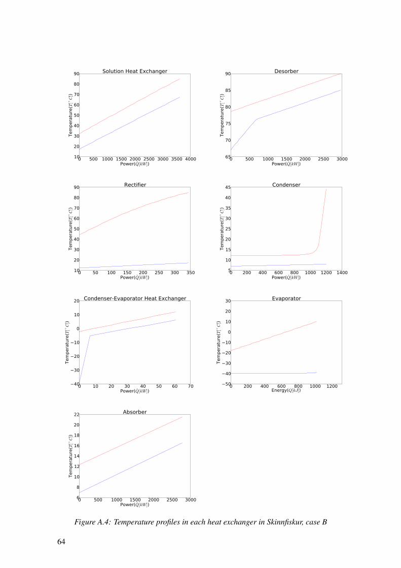
0 500 1000 1500 2000 2500 3000 3500 4000Power(Q[kW])

10

20

30

40

50

60

70

80

90Tem

pera

ture

(T[◦C

])Solution Heat Exchanger

0 500 1000 1500 2000 2500 3000Power(Q[kW])

65

70

75

80

85

90

Tem

pera

ture

(T[◦C

])

Desorber

0 50 100 150 200 250 300 350Power(Q[kW])

10

20

30

40

50

60

70

80

90

Tem

pera

ture

(T[◦C

])

Rectifier

0 200 400 600 800 1000 1200 1400Power(Q[kW])

5

10

15

20

25

30

35

40

45

Tem

pera

ture

(T[◦C

])

Condenser

0 10 20 30 40 50 60 70Power(Q[kW])

40

30

20

10

0

10

20

Tem

pera

ture

(T[◦C

])


0 200 400 600 800 1000 1200Energy(Q[kJ])

50

40

30

20

10

0

10

20

30

Tem

pera

ture

(T[◦C

])

Evaporator

0 500 1000 1500 2000 2500 3000Power(Q[kW])

6

8

10

12

14

16

18

20

22

Tem

pera

ture

(T[◦C

])

Absorber

Figure A.4: Temperature profiles in each heat exchanger in Skinnfiskur, case B

64

A.5. Freezing plant, Case C

Table A.5: Properties for each point in case C


1 70,93 -44,4 287,6 0,534 0,000 889,9 0,001 41,3 [0.326, 0.674] [0.9881, 0.0119]2 2682,95 -41,1 287,8 0,535 -0,302 890,7 0,001 41,3 [0.326, 0.674] [0.326, 0.674]3 2682,95 -36,3 288,9 0,551 -0,299 889,9 0,001 41,3 [0.326, 0.674] [0.326, 0.674]4 2682,95 273,6 358,0 1,512 -0,142 833,4 0,001 41,3 [0.326, 0.674] [0.326, 0.674]5 2682,95 550,7 415,9 2,229 -0,002 771,4 0,001 41,3 [0.326, 0.674] [0.326, 0.674]6 2682,95 688,9 425,3 2,557 0,067 172,3 0,006 41,3 [0.289, 0.711] [0.8403, 0.1597]7 2682,95 2023,8 425,3 6,308 1,000 14,6 0,069 2,8 [0.289, 0.711] [0.8403, 0.1597]8 2682,95 1286,0 368,4 4,459 0,649 26,5 0,038 2,8 [0.5687, 0.4313] [0.9868, 0.0132]9 800,00 1286,0 331,9 4,826 0,710 7,4 0,136 2,8 [0.4721, 0.5279] [0.991, 0.009]

10 800,00 1738,7 331,9 6,248 1,000 5,2 0,191 2,0 [0.4721, 0.5279] [0.991, 0.009]11 2682,95 593,0 425,3 2,288 0,000 776,7 0,001 38,6 [0.289, 0.711] [0.8403, 0.1597]12 2682,95 296,0 363,0 1,533 0,000 843,2 0,001 38,6 [0.289, 0.711] [0.289, 0.711]13 800,00 296,0 363,3 1,539 -0,010 842,0 0,001 38,6 [0.289, 0.711] [0.289, 0.711]14 800,00 179,7 331,9 1,351 0,000 800,9 0,001 0,1 [0.4723, 0.5277] [0.991, 0.009]15 800,00 295,8 363,3 1,539 -0,010 842,0 0,001 38,6 [0.2893, 0.7107] [0.2893, 0.7107]16 800,00 348,7 370,2 1,683 0,013 245,0 0,004 38,6 [0.2807, 0.7193] [0.9163, 0.0837]17 800,00 1890,3 370,2 6,608 1,000 4,7 0,215 0,5 [0.2807, 0.7193] [0.9163, 0.0837]18 800,00 1514,2 331,9 5,543 0,856 6,1 0,163 0,5 [0.4723, 0.5277] [0.9909, 0.0091]19 800,00 1738,7 331,9 6,248 1,000 5,2 0,191 0,4 [0.4721, 0.5279] [0.991, 0.009]20 800,00 327,6 370,2 1,616 0,000 838,9 0,001 38,1 [0.2807, 0.7193] [0.9163, 0.0837]21 800,00 -8,7 294,9 0,602 0,000 899,5 0,001 38,1 [0.2807, 0.7193] [0.2807, 0.7193]22 800,00 179,8 331,9 1,351 0,000 801,0 0,001 0,8 [0.4721, 0.5279] [0.991, 0.009]23 800,00 -4,8 295,9 0,620 -0,149 897,6 0,001 38,9 [0.2847, 0.7153] [0.2847, 0.7153]24 800,00 1738,7 331,9 6,248 1,000 5,2 0,191 2,4 [0.991, 0.009] [0.991, 0.009]25 800,00 398,1 287,2 1,694 0,000 622,9 0,002 2,4 [0.991, 0.009] [0.991, 0.009]26 800,00 290,8 264,0 1,305 0,000 654,9 0,001 2,4 [0.991, 0.009] [0.991, 0.009]27 70,93 290,8 233,1 1,346 0,100 6,3 0,159 2,4 [0.9899, 0.0101] [1.0, 0.0]28 70,93 1417,6 235,1 6,175 0,909 0,7 1,440 2,4 [0.89, 0.11] [1.0, 0.0]29 70,93 1524,8 261,3 6,175 999,000 0,0 0,000 2,4 [0.3984, 0.6016] [0.9909, 0.0091]30 70,93 -4,8 295,3 0,622 0,002 192,3 0,005 38,9 [0.2833, 0.7167] [0.9774, 0.0226]31 70,93 84,6 294,5 0,977 0,056 8,8 0,114 41,3 [0.2871, 0.7129] [0.9786, 0.0214]32 1900,00 896,7 482,9 2,423 0,000 853,0 0,001 22,7 [0.0, 1.0] [0.0, 1.0]33 1900,00 644,9 425,9 1,868 0,000 915,2 0,001 22,7 [0.0, 1.0] [0.0, 1.0]34 1900,00 39,7 282,2 0,136 0,000 1000,6 0,001 282,7 [0.0, 1.0] [0.0, 1.0]35 1900,00 39,7 282,2 0,136 0,000 1000,6 0,001 110,5 [0.0, 1.0] [0.0, 1.0]36 1900,00 69,0 289,2 0,239 0,000 999,8 0,001 110,5 [0.0, 1.0] [0.0, 1.0]

65

0 2000 4000 6000 8000 10000 12000 14000Energy(Q[kJ])

10

20

30

40

50

60

70

80

90

100

Tem

pera

ture

(T[◦C

])

Solution Heat Exchanger I

0 2000 4000 6000 8000 10000 12000Energy(Q[kJ])

80

90

100

110

120

130

140

150

160

Tem

pera

ture

(T[◦C

])

Solution Heat Exchanger II

0 50 100 150 200Energy(Q[kJ])

10

20

30

40

50

60

70

80

90

100

Tem

pera

ture

(T[◦C

])

Rectifier

0 500 1000 1500 2000 2500 3000 3500Power(Q[kW])

0

10

20

30

40

50

60

Tem

pera

ture

(T[◦C

])

Condenser

0 1000 2000 3000 4000 5000 6000Energy(Q[kJ])

140

150

160

170

180

190

200

210

Tem

pera

ture

(T[◦C

])

Generator I

0 500 1000 1500 2000 2500Energy(Q[kJ])

90

100

110

120

130

140

150

160

Tem

pera

ture

(T[◦C

])

Generator II

0 50 100 150 200 250 300Energy(Q[kJ])

40

30

20

10

0

10

20

Tem

pera

ture

(T[◦C

])


0 500 1000 1500 2000 2500 3000Energy(Q[kJ])

50

40

30

20

10

0

10

20

30

Tem

pera

ture

(T[◦C

])

Evaporator

0 1000 2000 3000 4000 5000 6000Energy(Q[kJ])

8

10

12

14

16

18

20

22

Tem

pera

ture

(T[◦C

])

Absorber

Figure A.5: Temperature profiles in each heat exchanger case C66

B. Programs

All the programming can be observed in this appendix.

B.1. Assumptions - Integral

from numpy import *import matplotlib.pyplot as pltimport csvimport datetime as dtimport matplotlib as mplfrom matplotlib.backends.backend_pdf import PdfPagesimport matplotlibmatplotlib.rcParams.update({’font.size’: 35})from scipy.integrate import simps, trapzi=0hiti=[]Dagsetning=[]with open(’nesfiskur/Rafmagn_ar.csv’, ’rb’) as csvfile:

spamreader = csv.reader(csvfile, delimiter=’;’)for row in spamreader:

try:h=float(row[2])hi=round(h,3)hiti.append(hi)Dagsetning.append(row[1])

except ValueError:pass

max=size(hiti)hitastig=[]dagur=[]k=0u=0for i in range(0,max):

if i%5 == 0:#90 er 4 gildi a dagk+=1if 47102<k<51470:#Few days 47102 to 51470

hitastig.append(hiti[i])dagur.append(Dagsetning[i])u+=1

print ’u:’ +str(u) +’ k: ’ + str(k)time_num_list = map(lambda x: mpl.dates.date2num(dt.datetime.strptime(x, ’%d.%m.%Y %H:%M:%S:%f’)),dagur)Time_from_zero=[]Time_hour=[]for s in range(0,u):

Time_from_zero.append(time_num_list[s]-time_num_list[0])Time_hour.append(Time_from_zero[s]*600/0.006944444379799998*1/3600)

print ’Fyrsti dagur: ’ +str(dagur[0]) +’ Sidasti dagur: ’ +str(dagur[u-1])Integralall=simps(hitastig, x=Time_hour)other=ones(size(Time_hour))*150intgrallother=simps(other, x=Time_hour)Integrall=Integralall-intgrallotherprint ’kWh: ’ + str(Integrall)#Klukkutimi:dx= 0.041667fig = plt.figure()plt.plot_date(x=time_num_list, y=hitastig, fmt="b-")fig.autofmt_xdate()plt.title("Temperature range in a freezer in Nesfiskur for few days in October")#Power in Nesfiskur for a yearplt.ylabel("Temperature[$^\circ C$]")#Power[$kW$]plt.grid(True)plt.show()

67

B.2. Programming for Case A

from numpy import *import matplotlib.pyplot as pltimport matplotlibfrom refprop import refpropfrom pprint import pprintimport pkg_resourcesfrom openpyxl.workbook import Workbookfrom openpyxl.writer.excel import ExcelWriterfrom openpyxl.cell import get_column_letterimport matplotlibmatplotlib.rcParams.update({’font.size’: 35})NUM_UNITS = 24NUM_water = 6KELVIN = 273.15cp_ammonia=2.19 #kJ/(kg K)cp_water=4.187 #kJ/(kg K)p_high=700aw=refprop(’ammonia.fld’,’water.fld’)def main():

vars = {}Q={}for i in range(1,NUM_UNITS + 1):

vars[i] = {’h’:0.0,’p’:0.0,’s’:0.0,’T’:0.0,’q’:0.0,’m’:0.0,’v’:0.0,’d’:0.0,’x’:[0.0,0.0],’y’:[0.0,0.0]}Q={’hx_1’:0.0,’Desorber’:0.0,’Hx_3’:0.0,’Condenser’:0.0,’Rectifier’:0.0,’Evaporator’:0.0,’a’:0.0, ’wdot_p’:0.0,

’Reykjanes’:0.0,’Absorber’:0.0,’Regenerator’:0.0,’Reykjanes’:0.0}Area={’SHX’:0.0,’Desorber’:0.0,’Hx_3’:0.0,’Condenser’:0.0,’Rectifier’:0.0,’Evaporator’:0.0, ’Absorber’:0.0,

’Regenerator’:0.0,’Reykjanes’:0.0}

NH3=0.33925639NH3=0.34x1=[NH3,(1-NH3)]p_high=700.467681706p_high=700#T6opt=373.0176149#NesfiskurT6opt=367.996437799#Skinnfiskur#m1=11.983125#Nesfiskurm1=9.00058285807#Skinnfiskurprint ’NH3: ’,NH3print ’p_high: ’,p_highprint ’T6opt: ’,T6optprint ’m1: ’,m1aw=refprop(’ammonia.fld’,’water.fld’)A = aw.thermo(’h’,t=285.15, p=p_high,x=[0.996,1-0.996] )h_low=A[0]A = aw.thermo(’p’,t=233.15, h=h_low,x=[0.996,1-0.996] )p_low=A[0]print p_lowvars[1] = {’p’:p_low}aw=refprop(’ammonia.fld’,’water.fld’)pr=1100#----------------------------------- Point 1 -----------------------------------------A = aw.thermo(’hpstqdxy’,q=0, p=vars[1][’p’],x=x1)[h, p, s, T, q, d, x, y] = A[0:8]if d==0:

v=0else:

v=1/dvars[1] = {’h’:h, ’p’:p, ’s’:s, ’T’:T,’v’:v, ’q’:q, ’d’:d ,’m’:m1,’x’:x, ’y’:y}#---------------------------------Point 2, Pump----------------------------vars[2] = {’p’:p_high, ’x’:x1}C = calculate_pump(vars[1][’p’], vars[2][’p’], vars[1][’m’],vars[1][’h’],vars[1][’v’],vars[1][’s’],vars[1][’x’])vars[2]=C[0]Q[’wdot_p’]=C[1][’wdot_p’]#--------------------------------Point 3 Hx_1------------------------------#Starting valuesm5=1.98x5=[0.5140202284,(1-0.5140202284)]vars[5]={’p’:vars[2][’p’], ’q’:0 , ’x’:x5}#Water at pressure 1555.576 and quality 0h3old=1500/(vars[2][’m’])+vars[2][’h’]A = aw.thermo(’hpstqdxy’,h=h3old, p=p_high,x=vars[2][’x’])[h, p, s, T, q, d, x, y] = A[0:8]vars[3] = {’h’:h, ’p’:p, ’s’:s, ’T’:T, ’q’:q, ’d’:d ,’m’:m1,’x’:x, ’y’:y}Dm5=1for i in range(0,4):

A = aw.thermo(’hpstqdxy’,q=1, p=p_high,x=[0.996,1-0.996] )[h, p, s, T, q, d, x, y] = A[0:8]v9=1/dvars[9] = {’h’:h, ’p’:p, ’s’:s, ’T’:T, ’q’:q,’v’:v9, ’d’:d, ’x’:x ,’y’:y}

vars[5]={’p’:vars[2][’p’], ’q’:0 , ’x’:x5}#Water at pressure 1555.576 and quality 0A = aw.thermo(’hpstqdxy’,q=vars[5][’q’], p=vars[5][’p’],x=x5 )[h, p, s, T, q, d, x, y] = A[0:8]v5=1/dvars[5] = {’h’:h, ’p’:p, ’s’:s, ’T’:T, ’q’:q, ’d’:d,’v’:v5, ’m’:m5, ’x’:x ,’y’:y}#Mixed fluidsvars[4]=calculate_mixed(vars[3],vars[5])#after heatingA = aw.thermo(’hpstqdxy’,t=T6opt, p=p_high,x=vars[4][’x’])[h, p, s, T, q, d, x, y] = A[0:8]m6=vars[4][’m’]

68

v6=1/dvars[6] = {’h’:h, ’p’:p, ’s’:s, ’T’:T, ’q’:q, ’d’:d, ’m’:m6,’v’:v6, ’x’:x ,’y’:y}#water from resevoirA = aw.thermo(’hpstqdxy’,p=vars[6][’p’], q=1 , x=vars[6][’y’])[h, p, s, T, q, d, x, y] = A[0:8]m7=vars[6][’m’]*vars[6][’q’]v7=1/dvars[7]={’h’:h, ’p’:p, ’s’:s, ’T’:T, ’q’:q,’v’:v7, ’d’:d,’x’:x, ’y’:y, ’m’:m7}A = aw.thermo(’hpstqdxy’,t=vars[9][’T’], p=p_high,x=vars[7][’y’] )[h, p, s, T, q, d, x, y] = A[0:8]m8=vars[7][’m’]v8=1/dvars[8] = {’h’:h, ’p’:p, ’s’:s, ’T’:T, ’q’:q,’v’:v8, ’d’:d,’m’:m8, ’x’:x ,’y’:y}Q[’Rectifier’]=vars[7][’m’]*(vars[7][’h’]-vars[8][’h’])h3n=Q[’Rectifier’]/(vars[2][’m’])+vars[2][’h’]A = aw.thermo(’hpstqdxy’,h=h3n, p=p_high,x=vars[2][’x’])[h, p, s, T, q, d, x, y] = A[0:8]v3=1/3vars[3] = {’h’:h, ’p’:p, ’s’:s, ’T’:T, ’q’:q,’v’:v3, ’d’:d ,’m’:m1,’x’:x, ’y’:y}m5=vars[8][’m’]*(1-vars[8][’q’])x5=vars[8][’x’]vars[9][’m’]=vars[8][’m’]*(vars[8][’q’])

#Liquid partA = aw.thermo(’hpstqdxy’,p=vars[6][’p’], q=0 , x=vars[6][’x’])[h, p, s, T, q, d, x, y] = A[0:8]v13=1/dvars[13]={’h’:h, ’p’:p, ’s’:s, ’T’:T, ’q’:q, ’v’:v13,’d’:d, ’x’:x, ’y’:y}vars[13][’m’]=vars[6][’m’]*(1-vars[6][’q’])#------------------------------ Condenser ------------------------------------#The sea is 7 degrees 273.15+7+5A = aw.thermo(’hpstqdxy’,p=vars[9][’p’], t=285.15,x=vars[9][’y’])[h, p, s, T, q, d, x, y] = A[0:8]m=vars[9][’m’]v10=1/dvars[10]= {’h’:h, ’p’:p, ’s’:s, ’T’:T, ’q’:q, ’x’:x, ’v’:v10, ’y’:y, ’d’:d,’m’:m}Q_c=vars[10][’m’]*(vars[9][’h’]-vars[10][’h’])Q[’Condenser’]=Q_c#---------------------------- Throttle ------------------------------------A = aw.thermo(’hpstqdxy’,p=p_low, h=vars[10][’h’],x=vars[10][’x’])[h, p, s, T, q, d,x,y] = A[0:8]v11=1/dvars[11]={’s’:s, ’T’:T, ’q’:q, ’d’:d, ’p’:p, ’v’:v11, ’m’:vars[10][’m’], ’h’:h, ’x’:x,’y’:y}#--------------------------- Evaporator -----------------------------------A = aw.thermo(’hpstqdxy’,t=vars[11][’T’]+5, p=p_low,x=vars[11][’x’])[h, p, s, T, q, d,x,y] = A[0:8]m12=vars[11][’m’]v12=1/dvars[12]= {’h’:h, ’p’:p, ’s’:s, ’T’:T, ’q’:q, ’x’:x, ’y’:y, ’v’:v12 ,’d’:d,’m’:m12}Q[’Evaporator’]=vars[12][’m’]*(vars[12][’h’]-vars[11][’h’])#-------------------------------Point 14 -----------------------------------------A=aw.thermo(’hpstqdxy’,p=p_low, h=vars[13][’h’],x=vars[13][’x’])[h, p, s, T, q, d,x,y] = A[0:8]if d==0:

v14=0.0else:

v14=1/dm=vars[13][’m’]vars[14]={’h’:h, ’p’:p, ’s’:s, ’T’:T, ’q’:q, ’d’:d, ’v’:v14, ’m’:m, ’x’:x , ’y’:y}#---------------------------------absorption mixed fluids ----------------------------------------#m_1*h_1+m_2*h_2=m_3*h_3m15=vars[12][’m’]+vars[14][’m’]h15=(vars[12][’m’]*vars[12][’h’]+vars[14][’m’]*vars[14][’h’])/m15A=aw.thermo(’hpstqdxy’,p=p_low, h=h15,x=vars[1][’x’])[h, p, s, T, q, d,x,y] = A[0:8]v15=1/dvars[15]={’h’:h, ’p’:p, ’s’:s, ’T’:T, ’q’:q, ’d’:d, ’v’:v15, ’m’:m15, ’x’:x , ’y’:y}#Absorber:Q[’Absorber’]=vars[1][’m’]*(vars[15][’h’]-vars[1][’h’])mr=13.3839443#Nesfiskurpr=1100w=refprop(’water.fld’)#Point 17Q[’Desorber’]=vars[4][’m’]*(vars[6][’h’]-vars[4][’h’])A=w.thermo(’hpstqdxy’,p=pr, t=160+273.15)[h, p, s, T, q, d] = A[0:6]m=mrv=1/dvars[16]={’h’:h, ’p’:p, ’s’:s, ’T’:T, ’q’:q, ’d’:d, ’v’:v,’m’:m, ’x’:[0.0,1.0] , ’y’:[0.0,1.0]}#Point 18h17=vars[16][’h’]-Q[’Desorber’]/mrA=w.thermo(’hpstqdxy’,p=pr, h=h17)[h, p, s, T, q, d] = A[0:6]m=mrv17=1/dvars[17]={’h’:h, ’p’:p, ’s’:s, ’T’:T, ’q’:q, ’d’:d, ’v’:v17,’m’:m, ’x’:[0.0,1.0] , ’y’:[0.0,1.0]}

#point 23

#COPCOP=Q[’Evaporator’]/(Q[’Desorber’]+Q[’wdot_p’])

#Condenser

69

pc=500Tc1=273.15+7A=w.thermo(’hpstqdxy’,p=pc, t=Tc1)[h, p, s, T, q, d] = A[0:6]mc=125v=1/dvars[19]={’h’:h, ’p’:p, ’s’:s, ’T’:T, ’q’:q, ’d’:d, ’v’:v,’m’:mc, ’x’:[0.0,1.0] , ’y’:[0.0,1.0]}

hc2=Q[’Condenser’]/mc+vars[19][’h’]A=w.thermo(’hpstqdxy’,p=pc, h=hc2)[h, p, s, T, q, d] = A[0:6]v=1/dvars[20]={’h’:h, ’p’:p, ’s’:s, ’T’:T, ’q’:q, ’d’:d, ’v’:v,’m’:mc, ’x’:[0.0,1.0] , ’y’:[0.0,1.0]}

A=w.thermo(’hpstqdxy’,p=pc, t=Tc1)[h, p, s, T, q, d] = A[0:6]#ma=80v=1/dvars[21]={’h’:h, ’p’:p, ’s’:s, ’T’:T, ’q’:q, ’d’:d, ’v’:v, ’x’:[0.0,1.0] , ’y’:[0.0,1.0]}

#h22=Q[’Absorber’]/ma+vars[21][’h’]

A=w.thermo(’hpstqdxy’,p=pc, t=vars[15][’T’]-5)[h, p, s, T, q, d] = A[0:6]v=1/dvars[22]={’h’:h, ’p’:p, ’s’:s, ’T’:T, ’q’:q, ’d’:d, ’v’:v, ’x’:[0.0,1.0] , ’y’:[0.0,1.0]}ma=Q[’Absorber’]/(vars[22][’h’]-vars[21][’h’])vars[21][’m’]=mavars[22][’m’]=ma

A=w.thermo(’hpstqdxy’,p=pc, t=Tc1)[h, p, s, T, q, d] = A[0:6]m18=vars[19][’m’]+vars[21][’m’]v=1/dvars[18]={’h’:h, ’p’:p, ’s’:s, ’T’:T, ’q’:q, ’d’:d, ’v’:v,’m’:m18, ’x’:[0.0,1.0] , ’y’:[0.0,1.0]}

’’’#Rectifierh22=Q[’Rectifier’]/mc+h21A=w.thermo(’hpstqdxy’,p=pc, h=h22)[h, p, s, T, q, d] = A[0:6]v=1/dvars[22]={’h’:h, ’p’:p, ’s’:s, ’T’:T, ’q’:q, ’d’:d, ’v’:v,’m’:mc, ’x’:[1.00,0.00] , ’y’:[1.00,0.00]}’’’#Evaporatorw=refprop(’air.ppf’)A=w.thermo(’hpstqdxy’,p=100, t=273.15+10)[h, p, s, T, q, d] = A[0:6]v=1/dvars[23]={’h’:h, ’p’:p, ’s’:s, ’T’:T, ’q’:q, ’d’:d, ’v’:v, ’x’:[0.0,1.0] , ’y’:[0.0,1.0]}#370m^3 af lofti

A=w.thermo(’hpstqdxy’,p=100, t=273.15-18)[h, p, s, T, q, d] = A[0:6]v=1/dm24=Q[’Evaporator’]/(vars[23][’h’]-h)vars[24]={’h’:h, ’p’:p, ’s’:s, ’T’:T,’m’:m24, ’q’:q, ’d’:d, ’v’:v, ’x’:[0.0,1.0] , ’y’:[0.0,1.0]}vars[23][’m’]=m24

aw=refprop(’ammonia.fld’,’water.fld’)#Areas calculated#Condenser(Shell and tube):BTUtoW=5.6783Uhx_1=1.1Ucond=(125*BTUtoW)/1000#Shell and tube exchanger, builditsolarUrect=(125*BTUtoW)/1000Ushx=2500/1000 #Plate, builditsolarUeva=(800+2500)/2*10**(-3)Uabs=(125*BTUtoW)/1000Udes=(125*BTUtoW)/1000print ’Ucond: ’, Ucondprint ’Urect: ’, Urectprint ’Ushx: ’, Ushxprint ’Ueva: ’, Uevaprint ’Uabs: ’, Uabsprint ’Udes: ’, UdesUreg=1.1#U-tube horizontal bundle#H-Horizontal, fixed or floating tube sheet#(Q,U,Th1,Th2,Tc1,Tc2):Area[’Condenser’]=HXarea(Q[’Condenser’],Ucond,vars[9],vars[10],vars[19],vars[20],’Condenser’)Area[’Rectifier’]=HXarea(Q[’Rectifier’],Urect,vars[7],vars[8],vars[2],vars[3],’Rectifier’)Area[’SHX’]=HXarea(Q[’SHX’],Ushx,vars[14],vars[15],vars[3],vars[4],’Solution Heat Exchanger’)Area[’Desorber’]=HXarea(Q[’Desorber’],Urect,vars[16],vars[17],vars[4],vars[6],’Desorber’)Area[’Evaporator’]=HXareaA(Q[’Evaporator’],Ueva,vars[23],vars[24],vars[11],vars[12],’Evaporator’)Area[’Absorber’]=HXareaE(Q[’Absorber’],Uabs,vars[15],vars[1],vars[21],vars[22],’Absorber’)#Solution Hx#print ’Area: ’ +str(Area)pprint(vars)pprint(Q)pprint(Area)print ’COP: ’ + str(COP)write_to_excel(vars)

def calculate_pump(p0, p1, m0, h0,v0,s0,x0):A = aw.thermo(’h’,s=s0, p=p1,x=x0)

70

h1 = A[0]eta_p=0.9h6nytt=h0+1/eta_p*(h1-h0)A = aw.thermo(’hpstqdxy’,p=p1, h=h6nytt,x=x0 )[h, p, s, T, q, d, x,y] = A[0:8]v=1/dwdot_p=(m0*v)*(p1-p0)/eta_pm = (m0 *h0+wdot_p)/hreturn ({’h’:h, ’p’:p, ’s’:s, ’T’:T, ’q’:q, ’x’:x, ’d’:d, ’v’:v, ’m’:m, ’y’:y},{’wdot_p’:wdot_p})

def calculate_mixed(vars1,vars2):

m1=vars1[’m’]m2=vars2[’m’]mt=m1+m2h3=(m1*vars1[’h’]+m2*vars2[’h’])/mtx3=(vars1[’x’][0]*m1+vars2[’x’][0]*m2)/((vars1[’x’][0]+vars1[’x’][1])*m1+(vars2[’x’][0]+vars2[’x’][1])*m2)

A = aw.thermo(’hpstqdxy’,h=h3, p=vars1[’p’],x=[x3,(1-x3)])[h, p, s, T, q, d, x,y] = A[0:8]

if d==0:v=0

else:v=1/d

return {’h’:h, ’p’:p, ’s’:s, ’T’:T, ’q’:q,’v’:v ,’x’:x, ’y’:y, ’d’:d, ’m’:mt}

def calculate_HX(Qhx,m1,h1,p,x1):

#Only the ammonia is calculated and its ratio is x1 of totalh2=(Qhx/m1)+h1A = aw.thermo(’hpstqdxy’,p=p, h=h2,x=x1)[h, p, s, T, q, d,x,y] = A[0:8]m=m1v=1/dreturn {’h’:h, ’p’:p, ’s’:s, ’T’:T, ’q’:q, ’v’:v , ’d’:d,’m’:m,’x’:x, ’y’:y}

def calculate_Evaporator(Qe,h1,m1,p1,x0):he=Qe/m1+h1A = aw.thermo(’hpstqdxy’,h=he, p=p1,x=x0)[h, p, s, T, q, d,x,y] = A[0:8]m=m1return{’h’:h, ’p’:p, ’s’:s, ’T’:T, ’q’:q, ’d’:d, ’m’:m, ’x’:x, ’y’:y}

def HXarea(Qtotal,U,varsh1,varsh2,varsc1,varsc2,string):aw=refprop(’ammonia.fld’,’water.fld’)n=50DQ=(Qtotal+0)/(n-1)Q=zeros((n))Q[0]=0Q[-1]=QtotalDTh=(varsh1[’T’]-varsh2[’T’])/nDTc=(varsc1[’T’]-varsc2[’T’])/nph=varsh1[’p’]pc=varsc1[’p’]mh=varsh1[’m’]mc=varsc1[’m’]yh=varsh1[’y’]yc=varsc1[’y’]xh=varsh1[’x’]xc=varsc1[’x’]xyh=xhxyc=xcqh=varsh1[’q’]qc=varsc1[’q’]

#--------------Enthalpy--------------#Hot solutionhh=zeros((n))hh[-1]=varsh1[’h’]hh[0]=varsh2[’h’]Dhh=(varsh1[’h’]-varsh2[’h’])/(n-1)#Cold solutionhc=zeros((n))hc[0]=varsc1[’h’]hc[-1]=varsc2[’h’]Dhc=(varsc2[’h’]-varsc1[’h’])/(n-1)#-------------Temperature----------------Th=zeros((n))Th[-1]=varsh1[’T’]-273.15Th[0]=varsh2[’T’]-273.15Tc=zeros((n))Tc[0]=varsc1[’T’]-273.15Tc[-1]=varsc2[’T’]-273.15LMTD=zeros((n-1))dA=zeros((n-1))for i in range(1,n-1):

#Hot#Hotif string==’Evaporator’:

aw=refprop(’air.ppf’)if qh>=1:

xyh=yhQ[i]=DQ*ihh[i]=+(hh[i-1])+Dhh

71

A=aw.thermo(’tyq’,p=ph, h=hh[i],x=xyh)Th[i]=A[0]-273.15yh=A[1]qh=A[2]aw=refprop(’ammonia.fld’,’water.fld’)#Coldif qc>=1:

xyc=ychc[i]=+(hc[i-1])+DhcB=aw.thermo(’tyq’,p=pc, h=hc[i],x=xyc)Tc[i]=B[0]-273.15yc=A[1]qc=A[2]

for k in range(1,n):LMTD[k-1]=((Th[k]-Tc[k])-(Th[k-1]-Tc[k-1]))/log((Th[k]-Tc[k])/(Th[k-1]-Tc[k-1]))dA[k-1]=DQ/(LMTD[k-1]*U)

A=sum(dA)plt.plot(Q,Th,’-r’,label=’Hot Solution’)plt.plot(Q,Tc,’-b’,label=’Cold Solution’)plt.title(string)plt.xlabel(’Energy($Q[kJ]$)’)plt.ylabel(’Temperature($T [^\circ C]$)’)plt.show()return A

def HXareaA(Qtotal,U,varsh1,varsh2,varsc1,varsc2,string):aw=refprop(’ammonia.fld’,’water.fld’)n=50DQ=(Qtotal+0)/(n-1)Qh=zeros((n))Qc=zeros((n))Qh[0]=0Qh[-1]=QtotalQc[0]=0Qc[-1]=QtotalDTh=(varsh1[’T’]-varsh2[’T’])/(n-1)DTc=(varsc2[’T’]-varsc1[’T’])/(n-1)ph=varsh1[’p’]pc=varsc1[’p’]mh=varsh1[’m’]mc=varsc1[’m’]yh=varsh1[’y’]yc=varsc1[’y’]xh=varsh1[’x’]xc=varsc1[’x’]xyh=xhxyc=xcqh=varsh1[’q’]qc=varsc1[’q’]

#--------------Enthalpy--------------#Hot solution

hh=zeros((n))hh[-1]=varsh1[’h’]hh[0]=varsh2[’h’]Dhh=(varsh1[’h’]-varsh2[’h’])/(n-1)

#Cold solutionhc=zeros((n))hc[0]=varsc1[’h’]hc[-1]=varsc2[’h’]Dhc=(varsc2[’h’]-varsc1[’h’])/(n-1)#-------------Temperature----------------Th=zeros((n))Th[-1]=varsh1[’T’]Th[0]=varsh2[’T’]

Thh=zeros((n))Thh[-1]=varsh1[’T’]-273.15Thh[0]=varsh2[’T’]-273.15

Tc=zeros((n))Tc[0]=varsc1[’T’]Tc[-1]=varsc2[’T’]

Tcc=zeros((n))Tcc[0]=varsc1[’T’]-273.15Tcc[-1]=varsc2[’T’]-273.15

LMTD=zeros((n-1))dA=zeros((n-1))for i in range(1,n-1):

#Hotif string==’Evaporator’:

aw=refprop(’air.ppf’)if qh>=1:

xyh=yh

Th[i]=+(Th[i-1])+DThA=aw.thermo(’hyqt’,p=ph, t=Th[i],x=xyh)Qh[i]=(A[0]-hh[0])*mhyh=A[1]qh=A[2]Thh[i]=Th[i]-273.15aw=refprop(’ammonia.fld’,’water.fld’)

72

#Coldif qc>=1:

xyc=ycTc[i]=+(Tc[i-1])+DTcB=aw.thermo(’hyq’,p=pc, t=Tc[i],x=xyc)hc[i]=B[0]Qc[i]=(B[0]-hc[0])*mcyc=B[1]qc=B[2]Tcc[i]=Tc[i]-273.15

for k in range(1,n):LMTD[k-1]=((Th[k]-Tc[k])-(Th[k-1]-Tc[k-1]))/log((Th[k]-Tc[k])/(Th[k-1]-Tc[k-1]))dA[k-1]=DQ/(LMTD[k-1]*U)

A=sum(dA)plt.plot(Qh,Thh,’-r’,label=’Hot Solution’)plt.plot(Qc,Tcc,’-b’,label=’Cold Solution’)plt.title(string)plt.xlabel(’Energy($Q[kJ]$)’)plt.ylabel(’Temperature($T [^\circ C]$)’)plt.show()return A

def HXareaE(Qtotal,U,varsh1,varsh2,varsc1,varsc2,string):aw=refprop(’ammonia.fld’,’water.fld’)n=2DQ=Qtotal/(n-1)Qh=zeros((n))Qc=zeros((n))Qh[0]=0Qc[0]=0Qh[-1]=QtotalQc[-1]=QtotalDTh=(varsh1[’T’]-varsh2[’T’])/nDTc=(varsc1[’T’]-varsc2[’T’])/n

#-------------Temperature----------------Th=zeros((n))Th[-1]=varsh1[’T’]-273.15Th[0]=varsh2[’T’]-273.15Tc=zeros((n))Tc[0]=varsc1[’T’]-273.15Tc[-1]=varsc2[’T’]-273.15DTc=(Tc[-1]-Tc[0])/(n-1)LMTD=zeros((n-1))dA=zeros((n-1))for k in range(1,n):

LMTD[k-1]=((Th[k]-Tc[k])-(Th[k-1]-Tc[k-1]))/log((Th[k]-Tc[k])/(Th[k-1]-Tc[k-1]))dA[k-1]=DQ/(LMTD[k-1]*U)

A=sum(dA)plt.plot(Qh,Th,’-r’,label=’Hot Solution’)plt.plot(Qc,Tc,’-b’,label=’Cold Solution’)plt.title(string)plt.xlabel(’Energy($Q[kJ]$)’)plt.ylabel(’Temperature($T [^\circ C]$)’)plt.show()return A

def write_to_excel(vars):wb = Workbook()dest_filename = ’FON_v5.xlsx’ws = wb.worksheets[0]ws.title = "First Option Nesfiskur"stafir=(’p’,’h’,’T’,’s’,’q’,’d’,’v’,’m’,’x’,’y’)colum = get_column_letter(1)ws.cell(row = 0, column = 0).value= ’Variables’ws.cell(row = 1, column = 0).value= ’p[kPa]’ws.cell(row = 2, column = 0).value= ’h[kJ/kg]’ws.cell(row = 3, column = 0).value= ’T[K]’ws.cell(row = 4, column = 0).value= ’s[kJ/K]’ws.cell(row = 5, column = 0).value= ’q’ws.cell(row = 6, column = 0).value= ’d[kg/m^3]’ws.cell(row = 7, column = 0).value= ’v[m^3/kg]’ws.cell(row = 8, column = 0).value= ’m[kg]’ws.cell(row = 9, column = 0).value= ’x’ws.cell(row = 10, column = 0).value= ’y’for col_idx in xrange(1, NUM_UNITS+1):

col = get_column_letter(col_idx+1)ws.cell(’%s%s’%(col,1)).value= ’%s’%(col_idx)for row in xrange(0,10):

if row < 8:ws.cell(’%s%s’%(col,row+2)).value= ’%s’%("{0:.3f}".format(round(vars[(col_idx)][stafir[row]],4)))

else:xy=vars[(col_idx)][stafir[row]]xy_0=xy[0]xy_1=xy[1]xy_f0=("%.4f" % xy_0)xy_f1=("%.4f" % xy_1)xy_f=[float(xy_f0),float(xy_f1)]ws.cell(’%s%s’%(col,row+2)).value= ’%s’%(xy_f)

ws = wb.create_sheet()wb.save(dest_filename)

if __name__ == "__main__":main()

73

B.3. Programming for Case B

from numpy import *import matplotlib.pyplot as pltimport matplotlibfrom refprop import refpropfrom pprint import pprintfrom openpyxl.workbook import Workbookfrom openpyxl.writer.excel import ExcelWriterfrom openpyxl.cell import get_column_letterimport matplotlibmatplotlib.rcParams.update({’font.size’: 22})NUM_UNITS = 30NUM_water = 6KELVIN = 273.15cp_ammonia=2.19 #kJ/(kg K)cp_water=4.187 #kJ/(kg K)p_low=71.661#p_low=70.9#p_high=670aw=refprop(’ammonia.fld’,’water.fld’)def main():

#------------------------------- Reykjanes ----------------------------------vars = {}Q={}for i in range(1,NUM_UNITS + 1):

vars[i] = {’h’:0.0,’p’:0.0,’s’:0.0,’T’:0.0,’q’:0.0,’m’:0.0,’v’:0.0,’d’:0.0,’x’:[0.0,0.0],’y’:[0.0,0.0]}Q={’SHX’:0.0,’Desorber’:0.0,’DesorberI’:0.0,’DesorberII’:0.0,’Hx_3’:0.0,’Condenser’:0.0,’Rectifier’:0.0,’Evaporator’:0.0,’CEHX’:0.0,

’wdot_p’:0.0,’Reykjanes’:0.0,’Absorber’:0.0,’Regenerator’:0.0,’Reykjanes’:0.0}Area={’SHX’:0.0,’Desorber’:0.0,’DesorberI’:0.0,’DesorberII’:0.0,’CEHX’:0.0,’Condenser’:0.0,’Rectifier’:0.0,’Evaporator’:0.0,

’Absorber’:0.0,’Regenerator’:0.0,’Reykjanes’:0.0}#m1=16.1531#Skinnfiskurm1=26.923#Q[’Desorber’]=2500#4500Q[’Rectifier’]=300#Q[’Evaporator’]=100#Q[’c’]x1=[0.34,(1-0.34)]vars[1] = {’p’:p_low}aw=refprop(’ammonia.fld’,’water.fld’)p_high=658

#----------------------------------- Point 1 -----------------------------------------A = aw.thermo(’hpstqdxy’,q=0, p=vars[1][’p’],x=x1)[h, p, s, T, q, d, x, y] = A[0:8]v=1/dvars[1] = {’h’:h, ’p’:p, ’s’:s, ’T’:T, ’q’:q, ’d’:d,’v’:v ,’m’:m1,’x’:x, ’y’:y}#--------------------------------- Point 2, Pump ----------------------------vars[2] = {’p’:p_high, ’x’:x1}C = calculate_pump(vars[1][’p’], vars[2][’p’], vars[1][’m’],vars[1][’h’],vars[1][’v’],vars[1][’s’],vars[1][’x’])vars[2]=C[0]Q[’wdot_p’]=C[1][’wdot_p’]print ’vars 2’print vars[2]#--------------------------------Point 3 Hx_1------------------------------#Starting valuesm16=vars[2][’m’]*0.9K=aw.thermo(’h’,q=0, p=vars[2][’p’],x=[0.3,1-0.3])h16=K[0]J=aw.thermo(’h’,t=(vars[2][’T’]+25), p=vars[2][’p’],x=[0.3,1-0.3])h17=J[0]#starting values for vars 5m6=0.05*m1x6=[0.5140202284,(1-0.5140202284)]vars[6]={’p’:vars[2][’p’], ’q’:0 , ’x’:x6}#Water at pressure 1555.576 and quality 0h3old=0.3*Q[’Desorber’]/(vars[2][’m’])+vars[2][’h’]A = aw.thermo(’hpstqdxy’,h=h3old, p=p_high,x=vars[2][’x’])[h, p, s, T, q, d, x, y] = A[0:8]v3=1/dvars[3] = {’h’:h, ’p’:p, ’s’:s, ’T’:T, ’q’:q, ’d’:d,’v’:v3 ,’m’:m1,’x’:x, ’y’:y}A = aw.thermo(’hpstqdxy’,t=65+273.15, p=p_high,x=vars[3][’x’])#x eitthvad annad[h, p, s, T, q, d, x, y] = A[0:8]v4=1/dvars[4] = {’h’:h, ’p’:p, ’s’:s, ’T’:T, ’q’:q, ’d’:d,’v’:v4 ,’m’:vars[3][’m’],’x’:x, ’y’:y}for i in range(0,4):

A = aw.thermo(’hpstqdxy’,q=1, p=p_high,x=[0.996,1-0.996] )[h, p, s, T, q, d, x, y] = A[0:8]v10=1/dvars[10] = {’h’:h, ’p’:p, ’s’:s, ’T’:T, ’q’:q, ’d’:d,’v’:v10, ’x’:x ,’y’:y}A = aw.thermo(’hpstqdxy’,q=vars[6][’q’], p=vars[6][’p’],x=x6 )[h, p, s, T, q, d, x, y] = A[0:8]v6=1/dvars[6] = {’h’:h, ’p’:p, ’s’:s, ’T’:T, ’q’:q, ’d’:d,’v’:v6, ’m’:m6, ’x’:x ,’y’:y}#Mixed fluidsvars[5]=calculate_mixed(vars[4],vars[6])#------------------------ Desorber -----------------------------#Liquid phase q=0 point 5sA = aw.thermo(’hpstqdxy’,q=0, p=p_high, x=vars[5][’x’])[h, p, s, T, q, d, x, y] = A[0:8]v29=1/dvars[29] = {’h’:h, ’p’:p, ’s’:s, ’T’:T, ’q’:q, ’d’:d,’v’:v29, ’m’:vars[5][’m’], ’x’:x ,’y’:y}A = aw.thermo(’hpstqdxy’,t=273.15+85, p=p_high, x=vars[5][’x’])[h, p, s, T, q, d, x, y] = A[0:8]

74

v7=1/dvars[7] = {’h’:h, ’p’:p, ’s’:s, ’T’:T, ’q’:q, ’d’:d,’v’:v7, ’m’:vars[5][’m’], ’x’:x ,’y’:y}Q[’DesorberI’]=vars[5][’m’]*(vars[29][’h’]-vars[5][’h’])Q[’DesorberII’]=vars[5][’m’]*(vars[7][’h’]-vars[29][’h’])A = aw.thermo(’hpstqdxy’,p=vars[7][’p’], q=1 , x=vars[7][’y’])[h, p, s, T, q, d, x, y] = A[0:8]v8=1/dm8=vars[7][’m’]*vars[7][’q’]vars[8]={’h’:h, ’p’:p, ’s’:s, ’T’:T, ’q’:q, ’d’:d, ’v’:v8,’x’:x, ’y’:y, ’m’:m8}A = aw.thermo(’hpstqdxy’,t=vars[10][’T’], p=p_high,x=vars[8][’y’] )[h, p, s, T, q, d, x, y] = A[0:8]v9=1/dm9=vars[8][’m’]vars[9] = {’h’:h, ’p’:p, ’s’:s, ’T’:T, ’q’:q, ’d’:d,’v’:v9,’m’:m9, ’x’:x ,’y’:y}Q[’Rectifier’]=vars[8][’m’]*(vars[8][’h’]-vars[9][’h’])h3n=Q[’Rectifier’]/(vars[2][’m’])+vars[2][’h’]A = aw.thermo(’hpstqdxy’,h=h3n, p=p_high,x=vars[2][’x’])[h, p, s, T, q, d, x, y] = A[0:8]v3=1/dvars[3] = {’h’:h, ’p’:p, ’s’:s, ’T’:T, ’q’:q, ’d’:d,’v’:v3 ,’m’:m1,’x’:x, ’y’:y}m6=vars[9][’m’]*(1-vars[9][’q’])x6=vars[9][’x’]vars[10][’m’]=vars[9][’m’]*(vars[9][’q’])#Liquid partA = aw.thermo(’hpstqdxy’,p=vars[7][’p’], q=0 , x=vars[7][’x’])[h, p, s, T, q, d, x, y] = A[0:8]v16=1/dvars[16]={’h’:h, ’p’:p, ’s’:s, ’T’:T, ’q’:q, ’v’:v16,’d’:d, ’x’:x, ’y’:y}vars[16][’m’]=vars[7][’m’]*(1-vars[7][’q’])#Point 17A = aw.thermo(’hpstqdxy’,p=vars[16][’p’], t=(vars[3][’T’]+15), x=vars[7][’x’])[h, p, s, T, q, d, x, y] = A[0:8]v17=1/dm=vars[16][’m’]vars[17]={’h’:h, ’p’:p, ’s’:s, ’T’:T, ’q’:q, ’d’:d,’v’:v17, ’x’:x, ’y’:y,’m’:m}h4=(vars[16][’m’]*(vars[16][’h’]-vars[17][’h’])/vars[3][’m’])+vars[3][’h’]Dh4=h4-vars[4][’h’]#print ’Dh4: ’,Dh4A = aw.thermo(’hpstqdxy’,h=h4, p=p_high,x=vars[3][’x’])#x eitthvad annad[h, p, s, T, q, d, x, y] = A[0:8]v4=1/dvars[4] = {’h’:h, ’p’:p, ’s’:s, ’T’:T, ’q’:q, ’d’:d,’v’:v7 ,’m’:vars[3][’m’],’x’:x, ’y’:y}

A = aw.thermo(’hpstqdxy’,p=p_low, h=vars[17][’h’], x=vars[7][’x’])[h, p, s, T, q, d, x, y] = A[0:8]if d==0:

v18=0else:

v18=1/dm=vars[17][’m’]vars[18]={’h’:h, ’p’:p, ’s’:s, ’T’:T, ’q’:q, ’d’:d,’v’:v18, ’x’:x, ’y’:y,’m’:m}Q[’SHX’]=vars[16][’m’]*(vars[16][’h’]-vars[17][’h’])#------------------------------ Condenser ------------------------------------#The sea is 7 degrees 273.15+7+5A = aw.thermo(’hpstqdxy’,p=vars[10][’p’], q=0, x=vars[10][’y’])[h, p, s, T, q, d, x, y] = A[0:8]m=vars[10][’m’]v11=1/dvars[11]= {’h’:h, ’p’:p, ’s’:s, ’T’:T, ’q’:q, ’x’:x, ’v’:v11, ’y’:y, ’d’:d,’m’:m}Q_c=vars[11][’m’]*(vars[10][’h’]-vars[11][’h’])Q[’Condenser’]=Q_ct12=270t15=350while(vars[11][’T’]<t15+6):

t12+=1A = aw.thermo(’hpstqdxy’,t=t12, p=p_high,x=vars[11][’x’])[h, p, s, T, q, d,x,y] = A[0:8]m12=vars[11][’m’]v12=1/dvars[12]= {’h’:h, ’p’:p, ’s’:s, ’T’:T, ’q’:q, ’x’:x, ’y’:y, ’v’:v12 ,’d’:d,’m’:m12}#---------------------------- Throttle ------------------------------------A = aw.thermo(’hpstqdxy’,p=p_low, h=vars[12][’h’],x=vars[12][’x’])[h, p, s, T, q, d,x,y] = A[0:8]if d==0:

v13=0else:

v13=1/dvars[13]={’s’:s, ’T’:T, ’q’:q, ’d’:d, ’p’:p, ’v’:v13, ’m’:vars[12][’m’], ’h’:h, ’x’:x,’y’:y}#--------------------------- Evaporator -----------------------------------A = aw.thermo(’hpstqdxy’,t=vars[13][’T’]+1, p=p_low,x=vars[13][’x’])[h, p, s, T, q, d,x,y] = A[0:8]m14=vars[13][’m’]if d==0:

v14=0else:

v14=1/dvars[14]= {’h’:h, ’p’:p, ’s’:s, ’T’:T, ’q’:q, ’x’:x, ’y’:y, ’v’:v14 ,’d’:d,’m’:m14}h15=(vars[11][’h’]-vars[12][’h’])+vars[14][’h’]A = aw.thermo(’hpstqdxy’,h=h15, p=p_low,x=vars[14][’x’])[h, p, s, T, q, d,x,y] = A[0:8]m15=vars[11][’m’]if d==0:

v15=0else:

v15=1/dvars[15]= {’h’:h, ’p’:p, ’s’:s, ’T’:T, ’q’:q, ’x’:x, ’y’:y, ’v’:v15 ,’d’:d,’m’:m15}

75

t15=vars[15][’T’]print ’T11: ’, vars[11][’T’]print ’T15: ’,vars[15][’T’]

Q[’Evaporator’]=vars[14][’m’]*(vars[14][’h’]-vars[13][’h’])#--------------CEHX--------------------Q[’CEHX’]=vars[11][’m’]*(vars[11][’h’]-vars[12][’h’])#---------------------------------absorption mixed fluids ----------------------------------------m19=vars[15][’m’]+vars[18][’m’]h19=(vars[15][’m’]*vars[15][’h’]+vars[18][’m’]*vars[18][’h’])/m19A=aw.thermo(’hpstqdxy’,p=p_low, h=h19,x=vars[1][’x’])[h, p, s, T, q, d,x,y] = A[0:8]v19=1/dvars[19]={’h’:h, ’p’:p, ’s’:s, ’T’:T, ’q’:q, ’d’:d, ’v’:v19, ’m’:m19, ’x’:x , ’y’:y}#Absorber:Q[’Absorber’]=vars[1][’m’]*(vars[19][’h’]-vars[1][’h’])pr=700w=refprop(’water.fld’)#Point 17A=w.thermo(’hpstqdxy’,p=pr, t=90+273.15)[h, p, s, T, q, d] = A[0:6]v=1/dvars[20]={’h’:h, ’p’:p, ’s’:s, ’T’:T, ’q’:q, ’d’:d, ’v’:v,’m’:m, ’x’:[0.0,1.0] , ’y’:[0.0,1.0]}#Point 18#---------------point 20s, thegar 5s q=0----------------------A=w.thermo(’hpstqdxy’,p=pr, t=vars[29][’T’]+5)[h, p, s, T, q, d] = A[0:6]mr=Q[’DesorberII’]/(vars[20][’h’]-h)m=mrv30=1/dvars[30]={’h’:h, ’p’:p, ’s’:s, ’T’:T, ’q’:q, ’d’:d, ’v’:v30,’m’:m, ’x’:[0.0,1.0] , ’y’:[0.0,1.0]}vars[20][’m’]=mrh21=vars[30][’h’]-Q[’DesorberI’]/mrA=w.thermo(’hpstqdxy’,p=pr, h=h21)[h, p, s, T, q, d] = A[0:6]v21=1/dvars[21]={’h’:h, ’p’:p, ’s’:s, ’T’:T, ’q’:q, ’d’:d, ’v’:v21,’m’:mr, ’x’:[0.0,1.0] , ’y’:[0.0,1.0]}print ’ mr: ’ +str(mr) + ’ pressure: ’+ str(p_high) + ’ Evaporator: ’+ str(Q[’Evaporator’])+’7q: ’ + str(vars[7][’q’])print ’ 13q and 14q: ’ +str(vars[13][’q’]) +’ and ’ + str(vars[14][’q’]) + ’ Evaporator temperature: ’ + str(vars[13][’T’])#point 23#COPCOP=Q[’Evaporator’]/(Q[’DesorberI’]+Q[’DesorberII’]+Q[’wdot_p’])#Condenserpc=500Tc1=273.15+7A=w.thermo(’hpstqdxy’,p=pc, t=Tc1)[h, p, s, T, q, d] = A[0:6]mc=290v=1/dvars[23]={’h’:h, ’p’:p, ’s’:s, ’T’:T, ’q’:q, ’d’:d, ’v’:v,’m’:mc, ’x’:[0.0,1.0] , ’y’:[0.0,1.0]}hc2=Q[’Condenser’]/mc+vars[23][’h’]A=w.thermo(’hpstqdxy’,p=pc, h=hc2)[h, p, s, T, q, d] = A[0:6]v=1/dvars[24]={’h’:h, ’p’:p, ’s’:s, ’T’:T, ’q’:q, ’d’:d, ’v’:v,’m’:mc, ’x’:[0.0,1.0] , ’y’:[0.0,1.0]}A=w.thermo(’hpstqdxy’,p=pc, t=Tc1)[h, p, s, T, q, d] = A[0:6]v=1/dvars[25]={’h’:h, ’p’:p, ’s’:s, ’T’:T, ’q’:q, ’d’:d, ’v’:v, ’x’:[0.0,1.0] , ’y’:[0.0,1.0]}A=w.thermo(’hpstqdxy’,p=pc, t=vars[19][’T’]-5)[h, p, s, T, q, d] = A[0:6]v=1/dma=Q[’Absorber’]/(vars[25][’h’]-vars[26][’h’])vars[25][’m’]=mavars[26]={’h’:h, ’p’:p, ’s’:s, ’T’:T, ’q’:q, ’d’:d, ’v’:v,’m’:ma, ’x’:[0.0,1.0] , ’y’:[0.0,1.0]}pc=500Tc1=273.15+7A=w.thermo(’hpstqdxy’,p=pc, t=Tc1)[h, p, s, T, q, d] = A[0:6]m=ma+mcv=1/dvars[22]={’h’:h, ’p’:p, ’s’:s, ’T’:T, ’q’:q, ’d’:d, ’v’:v,’m’:m, ’x’:[0.0,1.0] , ’y’:[0.0,1.0]}#Evaporatorw=refprop(’air.ppf’)#w=refprop(’water.fld’)A=w.thermo(’hpstqdxy’,p=100, t=273.15+10)[h, p, s, T, q, d] = A[0:6]v=0vars[27]={’h’:h, ’p’:p, ’s’:s, ’T’:T, ’q’:q, ’v’:v , ’d’:d, ’x’:[0.0,1.0] , ’y’:[0.0,1.0]}A=w.thermo(’hpstqdxy’,p=100, t=273.15-18)[h, p, s, T, q, d] = A[0:6]v=0m28=Q[’Evaporator’]/(vars[27][’h’]-h)vars[28]={’h’:h, ’p’:p, ’s’:s, ’T’:T,’m’:m28,’v’:v , ’q’:q, ’d’:d, ’x’:[0.0,1.0] , ’y’:[0.0,1.0]}vars[27][’m’]=m28Q[’Desorber’]=Q[’DesorberI’]+Q[’DesorberII’]aw=refprop(’ammonia.fld’,’water.fld’)#Areas calculated#Condenser(Shell and tube):Q[’SHXI’]=vars[14][’m’]*(vars[16][’h’]-vars[17][’h’])BTUtoW=5.6783Uhx_1=1.1Ucond=(125*BTUtoW)/1000#Shell and tube exchanger, builditsolarUrect=(125*BTUtoW)/1000Ushx=2500/1000 #Plate, builditsolarUeva=1.65

76

Uabs=(125*BTUtoW)/1000Udes=(125*BTUtoW)/1000Ucehx=(125*BTUtoW)/1000print ’Ucond: ’, Ucondprint ’Urect: ’, Urectprint ’Ushx: ’, Ushxprint ’Ueva: ’, Uevaprint ’Uabs: ’, Uabsprint ’Udes: ’, UdesUreg=1.1#U-tube horizontal bundle#H-Horizontal, fixed or floating tube sheet#(Q,U,Th1,Th2,Tc1,Tc2):Area[’Evaporator’]=HXareaA(Q[’Evaporator’],Ueva,vars[27],vars[28],vars[13],vars[14],’Evaporator’)Area[’Condenser’]=HXarea(Q[’Condenser’],Ucond,vars[10],vars[11],vars[23],vars[24],’Condenser’)Area[’CEHX’]=HXarea(Q[’CEHX’],Ucehx,vars[11],vars[12],vars[14],vars[15],’Condenser-Evaporator Heat Exchanger’)Area[’Rectifier’]=HXarea(Q[’Rectifier’],Urect,vars[8],vars[9],vars[2],vars[3],’Rectifier’)Area[’SHX’]=HXarea(Q[’SHX’],Ushx,vars[16],vars[17],vars[3],vars[4],’Solution Heat Exchanger’)Area[’Desorber’]=HXarea(Q[’Desorber’],Udes,vars[20],vars[21],vars[5],vars[7],’Desorber’)Area[’DesorberII’]=HXarea(Q[’DesorberII’],Udes,vars[20],vars[30],vars[29],vars[7],’Desorber II’)#Area[’Absorber’]=HXareaE(Q[’Absorber’],Uabs,vars[19],vars[1],vars[25],vars[26],’Absorber’)#plt.show()#Solution Hx#print ’Area: ’ +str(Area)pprint(vars)pprint(Q)pprint(Area)print ’COP: ’ + str(COP)

#----------The def function can be found in the programming in case 1if __name__ == "__main__":

main()

77

B.4. Programming for Case C

from numpy import *import matplotlib.pyplot as pltimport matplotlibfrom refprop import refpropfrom pprint import pprintfrom openpyxl.workbook import Workbookfrom openpyxl.writer.excel import ExcelWriterfrom openpyxl.cell import get_column_letterimport matplotlibmatplotlib.rcParams.update({’font.size’: 35})NUM_UNITS = 36NUM_water = 6Kelvin = 273.15cp_ammonia=2.19 #kJ/(kg K)cp_water=4.187 #kJ/(kg K)aw=refprop(’ammonia.fld’,’water.fld’)def main():

#------------------------------- Reykjanes ----------------------------------vars = {}Q={}for i in range(1,NUM_UNITS + 1):

vars[i] = {’h’:0.0,’p’:0.0,’s’:0.0,’T’:0.0,’q’:0.0,’m’:0.0,’v’:0.0,’d’:0.0,’x’:[0.0,0.0],’y’:[0.0,0.0]}Q={’SHXI’:0.0,’SHXII’:0.0,’GeneratorI’:0.0,’GeneratorII’:0.0,’Condenser’:0.0,’CondenserII’:0.0,’Rectifier’:0.0,

’RectifierII’:0.0,’Evaporator’:0.0,’CEHX’:0.0, ’wdot_p1’:0.0,’wdot_p’:0.0,’Reykjanes’:0.0,’AbsorberI’:0.0,’AbsorberII’:0.0,’Reykjanes’:0.0}Area={’SHXI’:0.0,’SHXII’:0.0,’GeneratorI’:0.0,’GeneratorII’:0.0,’DesorberII’:0.0,’CEHX’:0.0,’Condenser’:0.0,

’Rectifier’:0.0,’Evaporator’:0.0, ’Absorber’:0.0,’Regenerator’:0.0,’Reykjanes’:0.0}#Q[’Desorber’]=2500#4500#Q[’Rectifier’]=300#Q[’Evaporator’]=100#Q[’c’]’’’--------------Optimization----------------COP: 0.416021733401Evaporator: 588.507724076Generator I: 1382.021198x_1: [0.32599999999999996, 0.67400000000000004]x_rect1: [0.99095509860392428, 0.0090449013960757219]x_rect2: [0.99095509860392428, 0.0090449013960757219]p_h1: 2682.94832929p_h2: 800.0T6opt: 425.339890344T21opt: 6.0m1: 10-------------------------------------------’’’x_1=[0.326, 1-0.326]x_rect1=[0.99095509860392428,(1-0.99095509860392428)]x_rect2=[0.99095509860392428,(1-0.99095509860392428)]p_h1=2682.94832929p_h2=800.0pS=1900T_38=211+Kelvinm_1=41.330T6opt=425.339890344T21opt=6.0aw=refprop(’ammonia.fld’,’water.fld’)[hthrottle, xthottle] = aw.thermo(’hx’,t=273.15+9+5, p=p_h2,x=x_rect2)[p_low] = aw.thermo(’p’,h=hthrottle, t=233.15,x=xthottle)#----------------------------------- Point 1 -----------------------------------------[h, p, s, T, q, d, x, y] = aw.thermo(’hpstqdxy’,q=0, p=p_low,x=x_1)v=1/dvars[1] = {’h’:h, ’p’:p, ’s’:s, ’T’:T, ’q’:q, ’d’:d,’v’:v ,’m’:m_1,’x’:x, ’y’:y}print vars[1]#--------------------------------- Point 2, Pump ----------------------------------------------vars[2] = {’p’:p_h1, ’x’:x_1}C = calculate_pump(vars[1], vars[2])vars[2]=C[0]Q[’wdot_p’]=C[1][’wdot_p’]#--------------------------------- Point 6 , Generator I ---------------------------------------[h, p, s, T, q, d, x, y] = aw.thermo(’hpstqdxy’,t=T6opt, p=p_h1,x=vars[1][’x’])v6=1/dvars[6] = {’h’:h, ’p’:p, ’s’:s, ’T’:T, ’q’:q, ’d’:d,’v’:v6 ,’m’:vars[2][’m’],’x’:x, ’y’:y}#----------------------------- Vapor from seperator -------------------------------------------[h, p, s, T, q, d, x, y] = aw.thermo(’hpstqdxy’,p=p_h1, q=1 , x=vars[6][’y’])v7=1/dm7=vars[6][’m’]*vars[6][’q’]vars[7]={’h’:h, ’p’:p, ’s’:s, ’T’:T, ’q’:q, ’d’:d, ’v’:v7,’x’:x, ’y’:y, ’m’:m7}#-------------------------------Ammonia ratio rect_1 at point 9 ---------------------------------[h, p, s, T, q, d, x, y] = aw.thermo(’hpstqdxy’,q=1, p=p_h2,x=x_rect1)v10=1/dvars[10] = {’h’:h, ’p’:p, ’s’:s, ’T’:T, ’q’:q, ’d’:d,’v’:v10, ’x’:x ,’y’:y}#-------------------------------Generator II and throttle----------------------------[h, p, s, T, q, d, x, y] = aw.thermo(’hpstqdxy’,t=vars[10][’T’], p=p_h2,x=vars[7][’y’])v9=1/dm9=vars[7][’m’]vars[9] = {’h’:h, ’p’:p, ’s’:s, ’T’:T, ’q’:q, ’d’:d,’v’:v9,’m’:m9, ’x’:x ,’y’:y}vars[10][’m’]=m9*vars[9][’q’][h, p, s, T, q, d, x, y] = aw.thermo(’hpstqdxy’,p=p_h1, h=vars[9][’h’], x=vars[7][’y’])m=vars[7][’m’]v8=1/d

78

vars[8]= {’h’:h, ’p’:p, ’s’:s, ’T’:T, ’q’:q, ’x’:x, ’v’:v8, ’y’:y, ’d’:d,’m’:m}Q[’GeneratorII’]=vars[8][’m’]*(vars[7][’h’]-vars[8][’h’])#------------------------------------- Point 11 -------------------------------------------[h, p, s, T, q, d, x, y] = aw.thermo(’hpstqdxy’,p=p_h1, q=0 , x=vars[6][’x’])v11=1/dm11=vars[6][’m’]*(1-vars[6][’q’])vars[11]={’h’:h, ’p’:p, ’s’:s, ’T’:T, ’q’:q, ’d’:d, ’v’:v11,’x’:x, ’y’:y, ’m’:m11}#--------------------------------- Rectifier, point 19 ----------------------------------#Without massflow[h, p, s, T, q, d, x, y] = aw.thermo(’hpstqdxy’,q=1, p=p_h2,x=x_rect2)v19=1/dvars[19] = {’h’:h, ’p’:p, ’s’:s, ’T’:T, ’q’:q, ’d’:d,’v’:v19, ’x’:x ,’y’:y}# Iteration for Rectifier, SHXI and SHXII# Start valuesQ[’Rectifier’]=0.3*Q[’GeneratorII’]h3=Q[’Rectifier’]/vars[2][’m’]+vars[2][’h’][h3, T3, x3] = aw.thermo(’htx’,h=h3, p=p_h1,x=vars[2][’x’])[h21,T21, x21] = aw.thermo(’htx’,t=305, p=p_h2,x=[0.28,1-0.28])[h20,T20, x20] = aw.thermo(’htx’,q=0, p=p_h2,x=[0.28,1-0.28])T4guess=60vars[4][’T’]=T20-T4guess[h, p, s, T, q, d, x, y] = aw.thermo(’hpstqdxy’,q=0, p=p_h2,x=[0.514,(1-0.514)])m14=vars[2][’m’]*0.1vars[14] = {’h’:h, ’p’:p, ’s’:s, ’T’:T, ’q’:q, ’d’:d,’m’:m14, ’x’:x ,’y’:y}#vars[18][’x’]=[0.514,(1-0.514)]for i in range(0,4):

[h, p, s, T, q, d, x, y] = aw.thermo(’hpstqdxy’,t=vars[4][’T’]+5, p=p_h1,x=vars[11][’x’])v12=1/dm12=vars[11][’m’]vars[12] = {’h’:h, ’p’:p, ’s’:s, ’T’:T, ’q’:q, ’d’:d,’v’:v12,’m’:m12, ’x’:x ,’y’:y}Q[’SHXII’]=vars[12][’m’]*(vars[11][’h’]-vars[12][’h’])[h, p, s, T, q, d, x, y] = aw.thermo(’hpstqdxy’,h=vars[12][’h’], p=p_h2,x=vars[12][’x’])v13=1/dm13=vars[12][’m’]vars[13] = {’h’:h, ’p’:p, ’s’:s, ’T’:T, ’q’:q, ’d’:d,’v’:v13,’m’:m13, ’x’:x ,’y’:y}vars[15]=calculate_mixed(vars[14],vars[13])h16=vars[15][’h’]+Q[’GeneratorII’]/vars[15][’m’][h, p, s, T, q, d, x, y] = aw.thermo(’hpstqdxy’,h=h16, p=p_h2,x=vars[15][’x’])v16=1/dm16=vars[15][’m’]vars[16] = {’h’:h, ’p’:p, ’s’:s, ’T’:T, ’q’:q, ’d’:d,’v’:v16,’m’:m16, ’x’:x ,’y’:y}[h, p, s, T, q, d, x, y] = aw.thermo(’hpstqdxy’,q=1, p=p_h2,x=vars[16][’y’])v17=1/dm17=vars[16][’m’]*vars[16][’q’]vars[17] = {’h’:h, ’p’:p, ’s’:s, ’T’:T, ’q’:q, ’d’:d,’v’:v17,’m’:m17, ’x’:x ,’y’:y}[h, p, s, T, q, d, x, y] = aw.thermo(’hpstqdxy’,t=vars[19][’T’], p=p_h2,x=vars[17][’y’])v18=1/dvars[18] = {’h’:h, ’p’:p, ’s’:s, ’T’:T, ’q’:q, ’d’:d,’v’:v18, ’x’:x ,’y’:y}Q[’Rectifier’]=vars[17][’m’]*(vars[17][’h’]-vars[18][’h’])vars[18][’m’]=vars[17][’m’][h, p, s, T, q, d, x, y] = aw.thermo(’hpstqdxy’,q=0, p=p_h2,x=vars[18][’x’])v14=1/dm14=vars[18][’m’]*(1-vars[18][’q’])vars[14] = {’h’:h, ’p’:p, ’s’:s, ’T’:T, ’q’:q, ’d’:d,’v’:v14,’m’:m14, ’x’:x ,’y’:y}[h, p, s, T, q, d, x, y] = aw.thermo(’hpstqdxy’,q=0, p=p_h2,x=vars[16][’x’])v20=1/dm20=vars[16][’m’]*(1-vars[16][’q’])vars[20] = {’h’:h, ’p’:p, ’s’:s, ’T’:T, ’q’:q, ’d’:d,’v’:v20,’m’:m20, ’x’:x ,’y’:y}h3=Q[’Rectifier’]/vars[2][’m’]+vars[2][’h’][h, p, s, T, q, d, x, y] = aw.thermo(’hpstqdxy’,h=h3, p=p_h1,x=vars[2][’x’])v3=1/dm3=vars[2][’m’]vars[3] = {’h’:h, ’p’:p, ’s’:s, ’T’:T, ’q’:q, ’d’:d,’v’:v3,’m’:m3, ’x’:x ,’y’:y}[h, p, s, T, q, d, x, y] = aw.thermo(’hpstqdxy’,t=vars[3][’T’]+T21opt, p=p_h2,x=vars[20][’x’])v21=1/dm21=vars[20][’m’]vars[21] = {’h’:h, ’p’:p, ’s’:s, ’T’:T, ’q’:q, ’d’:d,’v’:v3,’m’:m21, ’x’:x ,’y’:y}Q[’SHXI’]=vars[21][’m’]*(vars[20][’h’]-vars[21][’h’])h4=vars[3][’h’]+Q[’SHXI’]/vars[3][’m’][h, p, s, T, q, d, x, y] = aw.thermo(’hpstqdxy’,h=h4, p=p_h1,x=vars[3][’x’])v4=1/dm4=vars[2][’m’]vars[4] = {’h’:h, ’p’:p, ’s’:s, ’T’:T, ’q’:q, ’d’:d,’v’:v4,’m’:m4, ’x’:x ,’y’:y}

h5=vars[4][’h’]+Q[’SHXII’]/vars[4][’m’][h, p, s, T, q, d, x, y] = aw.thermo(’hpstqdxy’,h=h5, p=p_h1,x=vars[4][’x’])v5=1/dm5=vars[4][’m’]vars[5] = {’h’:h, ’p’:p, ’s’:s, ’T’:T, ’q’:q, ’d’:d,’v’:v5,’m’:m5, ’x’:x ,’y’:y}[h, p, s, T, q, d, x, y] = aw.thermo(’hpstqdxy’,q=0, p=p_h2,x=vars[9][’x’])v22=1/dm22=vars[9][’m’]*(1-vars[9][’q’])vars[22] = {’h’:h, ’p’:p, ’s’:s, ’T’:T, ’q’:q, ’d’:d,’v’:v22,’m’:m22, ’x’:x ,’y’:y}vars[23]=calculate_mixed(vars[21],vars[22])vars[19][’m’]=vars[18][’m’]*vars[18][’q’]vars[24]=calculate_mixedvapor(vars[10],vars[19])#----------------------------Generator I --------------------------------Q[’GeneratorI’]=vars[5][’m’]*(vars[6][’h’]-vars[5][’h’])aw=refprop(’water.fld’)[h, p, s, T, q, d, x, y] = aw.thermo(’hpstqdxy’,q=0, p=pS)v=1/dvars[32] = {’h’:h, ’p’:p, ’s’:s, ’T’:T, ’q’:q, ’d’:d,’v’:v ,’x’:[0.0,1.0] , ’y’:[0.0,1.0]}[h, p, s, T, q, d, x, y] = aw.thermo(’hpstqdxy’,t=vars[5][’T’]+10, p=pS)v=1/dvars[33] = {’h’:h, ’p’:p, ’s’:s, ’T’:T, ’q’:q, ’d’:d,’v’:v ,’x’:[0.0,1.0] , ’y’:[0.0,1.0]}vars[33][’m’]=Q[’GeneratorI’]/(vars[32][’h’]-vars[33][’h’])

79

vars[32][’m’]=vars[33][’m’]aw=refprop(’ammonia.fld’,’water.fld’)#--------------------------- Condenser ----------------------------------A = aw.thermo(’hpstqdxy’,p=p_h2, t=287.15, x=vars[24][’y’])[h, p, s, T, q, d, x, y] = A[0:8]m=vars[24][’m’]v25=1/dvars[25]={’h’:h, ’p’:p, ’s’:s, ’T’:T, ’q’:q, ’d’:d,’v’:v25, ’x’:x, ’y’:y,’m’:m}#-----------------------Prufa----------------------t26=263t29=350while(vars[25][’T’]<t29+5):

t26+=1#A = aw.thermo(’h’,t=233.15, p=p_low,x=vars[11][’x’])#h12 = A[0]A = aw.thermo(’hpstqdxy’,t=t26, p=p_h2,x=vars[25][’x’])[h, p, s, T, q, d,x,y] = A[0:8]m26=vars[25][’m’]v26=1/dvars[26]= {’h’:h, ’p’:p, ’s’:s, ’T’:T, ’q’:q,’v’:v, ’x’:x, ’y’:y ,’d’:d,’m’:m26}#---------------------------- Throttle ------------------------------------A = aw.thermo(’hpstqdxy’,p=p_low, h=vars[26][’h’],x=vars[26][’x’])[h, p, s, T, q, d,x,y] = A[0:8]if d==0:

v27=0else:

v27=1/dvars[27]={’s’:s, ’T’:T, ’q’:q, ’d’:d, ’p’:p, ’v’:v27, ’m’:vars[26][’m’], ’h’:h, ’x’:x,’y’:y}#--------------------------- Evaporator -----------------------------------A = aw.thermo(’hpstqdxy’,t=vars[27][’T’]+2, p=p_low,x=vars[27][’x’])[h, p, s, T, q, d,x,y] = A[0:8]m28=vars[27][’m’]if d==0:

v28=0else:

v28=1/dvars[28]= {’h’:h, ’p’:p, ’s’:s, ’T’:T, ’q’:q, ’x’:x, ’y’:y, ’v’:v28 ,’d’:d,’m’:m28}

h29=(vars[25][’h’]-vars[26][’h’])+vars[28][’h’]A = aw.thermo(’hpstqdxy’,h=h29, p=p_low,x=vars[27][’x’])[h, p, s, T, q, d,x,y] = A[0:8]m29=vars[28][’m’]v=0vars[29]= {’h’:h, ’p’:p, ’s’:s, ’T’:T, ’q’:q,’v’:v, ’x’:x, ’y’:y ,’d’:d,’m’:m29}t29=vars[29][’T’]

Q[’Evaporator’]=vars[28][’m’]*(vars[28][’h’]-vars[27][’h’])COP=Q[’Evaporator’]/(Q[’GeneratorI’]+Q[’wdot_p’])Q[’CEHX’]=vars[25][’m’]*(vars[25][’h’]-vars[26][’h’])#---------------------------------absorption mixed fluids ----------------------------------------[h, p, s, T, q, d,x,y] = aw.thermo(’hpstqdxy’,p=p_low, h=vars[23][’h’],x=vars[23][’x’])if d==0:

v30=0else:

v30=1/dvars[30]={’h’:h, ’p’:p, ’s’:s, ’T’:T, ’q’:q, ’d’:d, ’v’:v30, ’m’:vars[23][’m’], ’x’:x , ’y’:y}m31=vars[29][’m’]+vars[30][’m’]h31=(vars[30][’m’]*vars[30][’h’]+vars[29][’m’]*vars[29][’h’])/m31[h, p, s, T, q, d,x,y] = aw.thermo(’hpstqdxy’,p=p_low, h=h31,x=vars[1][’x’])v31=1/dvars[31]={’h’:h, ’p’:p, ’s’:s, ’T’:T, ’q’:q, ’d’:d, ’v’:v31, ’m’:m31, ’x’:x , ’y’:y}#Absorber:Q[’Absorber’]=vars[1][’m’]*(vars[31][’h’]-vars[1][’h’])#CondenserQ[’Condenser’]=vars[24][’m’]*(vars[24][’h’]-vars[25][’h’])#Sea coolantaw=refprop(’water.fld’)[h, p, s, T, q, d, x, y] = aw.thermo(’hpstqdxy’,t=Kelvin+9, p=pS)v=1/dvars[34] = {’h’:h, ’p’:p, ’s’:s, ’T’:T, ’q’:q, ’d’:d,’v’:v ,’x’:[0.0,1.0] , ’y’:[0.0,1.0]}#condenser[h, p, s, T, q, d, x, y] = aw.thermo(’hpstqdxy’,t=Kelvin+9, p=pS)v=1/dvars[35] = {’h’:h, ’p’:p, ’s’:s, ’T’:T, ’q’:q, ’d’:d,’v’:v ,’x’:[0.0,1.0] , ’y’:[0.0,1.0]}[h, p, s, T, q, d, x, y] = aw.thermo(’hpstqdxy’,t=273.15+16, p=pS)v=1/dvars[36] = {’h’:h, ’p’:p, ’s’:s, ’T’:T, ’q’:q, ’d’:d,’v’:v ,’x’:[0.0,1.0] , ’y’:[0.0,1.0]}mc=(Q[’Condenser’])/(vars[36][’h’]-vars[35][’h’])vars[36][’m’]=mcvars[35][’m’]=mc[h, p, s, T, q, d, x, y] = aw.thermo(’hpstqdxy’,t=Kelvin+9, p=pS)v=1/dvars[37] = {’h’:h, ’p’:p, ’s’:s, ’T’:T, ’q’:q, ’d’:d,’v’:v ,’x’:[0.0,1.0] , ’y’:[0.0,1.0]}[h, p, s, T, q, d, x, y] = aw.thermo(’hpstqdxy’,t=vars[31][’T’]-5, p=pS)v=1/dvars[38] = {’h’:h, ’p’:p, ’s’:s, ’T’:T, ’q’:q, ’d’:d,’v’:v ,’x’:[0.0,1.0] , ’y’:[0.0,1.0]}mc2=(Q[’Absorber’])/(vars[38][’h’]-vars[37][’h’])vars[38][’m’]=mc2vars[37][’m’]=mc2vars[34][’m’]=mc+mc2#Evaporatorw=refprop(’air.ppf’)A=w.thermo(’hpstqdxy’,p=100, t=273.15+10)[h, p, s, T, q, d] = A[0:6]v=0vars[39]={’h’:h, ’p’:p, ’s’:s, ’T’:T, ’q’:q, ’v’:v , ’d’:d, ’x’:[0.0,1.0] , ’y’:[0.0,1.0]}

80

#370m^3 af loftiA=w.thermo(’hpstqdxy’,p=100, t=273.15-18)[h, p, s, T, q, d] = A[0:6]v=0m40=Q[’Evaporator’]/(vars[39][’h’]-h)vars[40]={’h’:h, ’p’:p, ’s’:s, ’T’:T,’m’:m40,’v’:v , ’q’:q, ’d’:d, ’x’:[0.0,1.0] , ’y’:[0.0,1.0]}vars[39][’m’]=m40aw=refprop(’ammonia.fld’,’water.fld’)BTUtoW=5.6783Uhx_1=1.1Ucond=(125*BTUtoW)/1000#Shell and tube exchanger, builditsolarUrect=(125*BTUtoW)/1000Ushx=2500/1000 #Plate, builditsolarUeva=1.65Uabs=(125*BTUtoW)/1000Udes=(125*BTUtoW)/1000Ucehx=(125*BTUtoW)/1000Area[’Evaporator’]=HXareaA(Q[’Evaporator’],Ueva,vars[39],vars[40],vars[27],vars[28],’Evaporator’)Area[’Condenser’]=HXarea(Q[’Condenser’],Ucond,vars[24],vars[25],vars[35],vars[36],’Condenser’)Area[’Rectifier’]=HXareaE(Q[’Rectifier’],Urect,vars[17],vars[18],vars[2],vars[3],’Rectifier’)Area[’SHXI’]=HXareaE(Q[’SHXI’],Ushx,vars[20],vars[21],vars[3],vars[4],’Solution Heat Exchanger I’)Area[’SHXII’]=HXareaE(Q[’SHXII’],Ushx,vars[11],vars[12],vars[4],vars[5],’Solution Heat Exchanger II’)Area[’GeneratorI’]=HXareaE(Q[’GeneratorI’],Udes,vars[32],vars[33],vars[5],vars[6],’Generator I’)Area[’GeneratorII’]=HXareaE(Q[’GeneratorII’],Udes,vars[7],vars[8],vars[15],vars[16],’Generator II’)Area[’CEHX’]=HXareaE(Q[’CEHX’],Ucehx,vars[25],vars[26],vars[28],vars[29],’Condenser-Evaporator Heat Exchanger’)Area[’Absorber’]=HXareaE(Q[’Absorber’],Uabs,vars[31],vars[1],vars[37],vars[38],’Absorber’)#plt.show()#Solution Hxprint ’Area: ’ +str(Area)pprint(vars)pprint(Q)pprint(Area)print ’COP: ’,COP#pprint(vars)write_to_excel(vars)#pprint(Q)

#Sem def’s as in program for case 1

81

B.5. Pressure drop

------------------Pressure drop calculations --------------------from numpy import *g=9.82d=[0.125,0.150,0.20,0.25,0.3]#G=0.014745 #nesfiskur#G=16.6*0.001 #skinnfiskurG=24.065*0.001 #TotalG=170.98*0.001 #case 2#G=32.616*0.001 #Totalrho=965.58#rho=907.73743#p=1100n=5Inew=zeros((n))Iold=25L=1u=zeros((n))f=ones((n))*nhloss=zeros((n))Re=zeros((n))hf=zeros((n))#k=0.0048*0.001k=0.001*0.001#Kinematic viscocityv=1.87753*10**(-7)#v=1*10**(-6)for i in range(0,n):

for h in range(1,15):Inew[i]=(1.072*(G)**2)/(g*(d[i])**5*(log(0.27*k/d[i]+1.78*v/sqrt(g*d[i]**3*Iold)))**2)Iold=Inew[i]Re[i]=(4*G)/(v*pi*d[i])s=-2.0*log10((k/d[i])/3.7+2.51/(Re[i]*sqrt(f[i])))f[i]=1/(s**2)

u[i]=(4*G)/(pi*d[i]**2)Re[i]=(4*G)/(v*pi*d[i])hloss[i]=f[i]*(L/d[i])*(u[i]**2)/2*rho

print ’Inew: ’,Inewprint ’hloss: ’,hlossprint ’u: ’,uprint ’Re: ’,Reprint ’f: ’,f

82

faculty of industrial engineering, mechanical engineering and

Documents