families of lines: random effects in linear regression

Families of lines: random effects in linear regression analysis

HENRY A. FELDMAN Department of Environmental Science and Physiology (Respiratory Biology Program), and Department of Biostatistics, Harvard University School of Public Health, Boston, Massachusetts 02115

FELDMAN, HENRY A. Families of lines: random effects in linear regression analysis. J. Appl. Physiol. 64(4): 1721-1732, 1988.-Laboratory experiments often involve two groups of subjects, with a linear phenomenon observed in each subject. Simple linear regression as propounded in standard textbooks is inadequate to treat this experimental design, particularly when it comes to dealing with random variation of slopes and intercepts among subjects. The author describes several techniques that can be used to compare two independent families of lines and illustrates their use with laboratory data. The methods are described tutorially, compared, and discussed in the context of more sophisticated and more naive approaches to this common data-analytic problem. Technical details are supplied in APPENDIX A.

statistics; data analysis

EVERYONE KNOWS how to fit a straight line to data. Simple linear regression is covered in every introductory statistics course and just as often in undergraduate phys- ics, psychology, or biochemistry. The geometry of linear regression is easily grasped. Its calculations are straight- forward, and its utility is evident in every branch of science. A routine for simple linear regression is included in even the most minimal statistical software package, whether for mainframe or microcomputer. Many pocket calculators have linear regression hard wired.

Thus it may seem that in this area of statistics the average scientist is adequately trained to analyze his own data. In practice, however, this is rarely the case, as the author has observed over some years as consultant and statistician-in-residence in a large academic department of physiology.

What stumps the average investigator is that linear regressions do not always come up one at a time. In the typical textbook example an entire experiment is encom- passed by one linear relationship. The result is one slope, one intercept, and one cogent test of the experimenter’s hypothesis. In practice things are not so simple. It does not take a very complex experiment to present the investigator with a lapful of different regression lines and a headful of questions.

Modern digital equipment contributes to this problem

by turning out great quantities of raw data, ready for processing. A subject is hooked up to a physiological monitor and produces a linear recording. For the sake of replication the line is repeated. Now the temperature is raised or the drug administered, and several more lines are recorded. Another subject is tested in the same way. One month and 20 subjects later, the data are complete.

Now what? Should simple linear regression be applied to each linear recording, or should each subject’s lines be combined? If so, how? By pooling the data points? By averaging x’s, or averaging y’s? What about two groups of subjects tested under different experimental conditions? What about the same subjects tested under different experimental conditions?

In this paper we provide firm answers to most of these questions by describing and comparing some data-analytic procedures for dealing with groups of regression lines. This article is written for scientists who find elementary statistics limiting but are not up to extracting the pertinent practical procedure from an advanced text or statistical literature. By providing an introduction to pertinent statistical techniques, the author hopes not to turn those readers into self-sufficient statisticians but to help them make use of statistical collaborators more frequently and fruitfully.

We pay particular attention to the treatment of random effects. By “random effects” we mean unmeasured, uncontrolled sources of variability that have a systematic influence on some portion of the experiment such as one day’s or one subject’s data. For example, physical fitness varies randomly among subjects in a physiological study, imparting a systematic bias to one person’s muscular length-tension relationship or the relation of his heart rate to exertion. The random effect of fitness cannot be removed by any sort of statistical adjustment because fitness is a difficult attribute to quantify, not being very well predicted by age, body type, or any other measurement independent of the study. The same can be said of many factors that must be written off as “biological variability.” A second important source of random effects is artifact, such as instrument bias, inconsistency of chemical batches, or simple unexplained daily fluctua- tions.

0161-7567/88 $1.50 Copyright 0 1988 the American Physiological Society 1721

1722 FAMILIES OF LINES

The theoretical approach inherent in the random- effects regression methods described below is to build the familiar experimental designs-two independent samples, one-way analysis of variance, etc.-not out of single numbers but out of regression lines. This approach is not found in basic statistics texts. Some of it falls within the classical theory of linear models as taught at the graduate level (19). Other aspects are the subject of current meth- odological research (1,8,9, 11,12,16,20,21). This paper is confined to the case of two groups to keep the mathematical notation clear. The same approach may be applied to experiments with more superstructure (three groups, two-factor design), more fine structure (nesting, replication), or partial constraint (parallel lines).

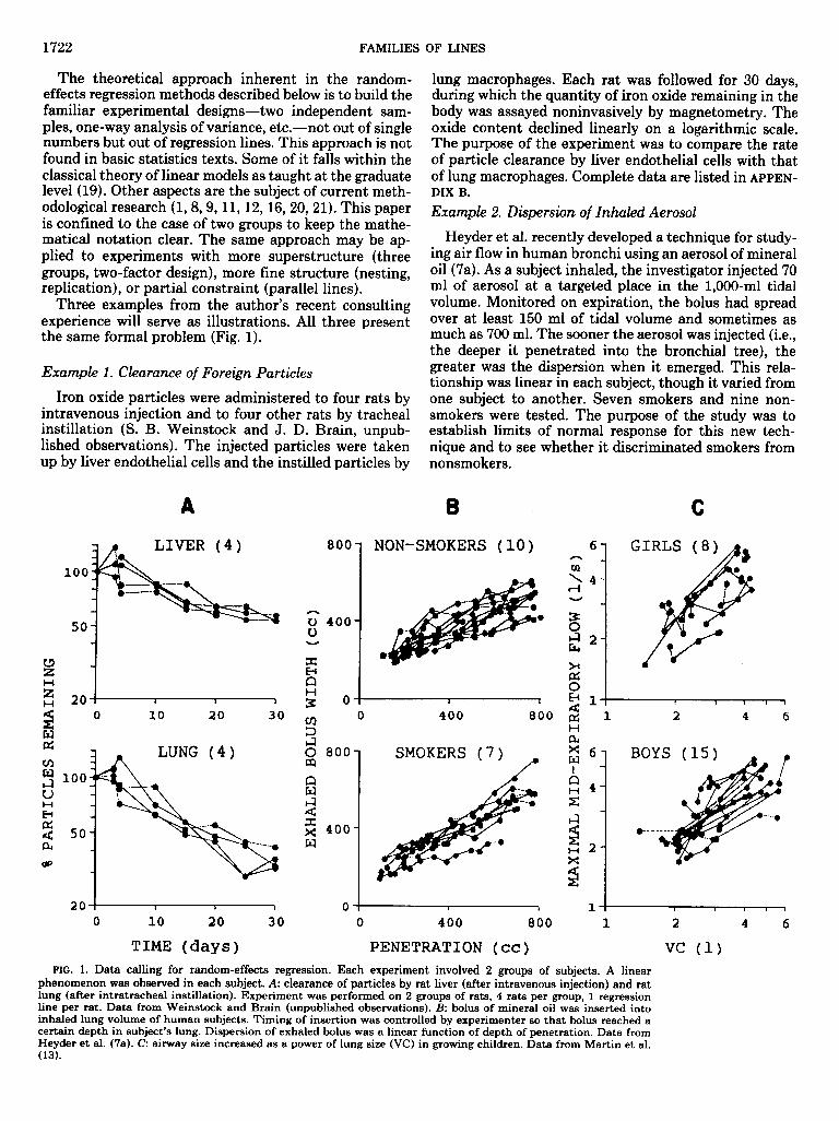
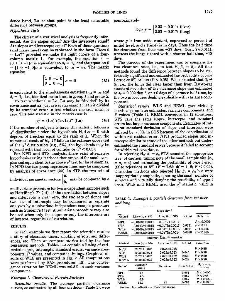
Three examples from the author’s recent consulting experience will serve as illustrations. All three present the same formal problem (Fig. 1).

lung macrophages. Each rat was followed for 30 days, during which the quantity of iron oxide remaining in the body was assayed noninvasively by magnetometry. The oxide content declined linearly on a logarithmic scale. The purpose of the experiment was to compare the rate of particle clearance by liver endothelial cells with that of lung macrophages. Complete data are listed in APPEN- DIX B.

Example 2. Dispersion of Inhaled Aerosol

Heyder et al. recently developed a technique for study- ing air flow in human bronchi using an aerosol of mineral oil (7a). As a subject inhaled, the investigator injected 70 ml of aerosol at a targeted place in the 1,000-ml tidal volume. Monitored on expiration, the bolus had spread over at least 150 ml of tidal volume and sometimes as much as 700 ml. The sooner the aerosol was injected (i.e., the deeper it penetrated into the bronchial tree), the greater was the dispersion when it emerged. This relationship was linear in each subject, though it varied from one subject to another. Seven smokers and nine nonsmokers were tested. The purpose of the study was to establish limits of normal response for this new technique and to see whether it discriminated smokers from nonsmokers.

Example 1. Clearance of Foreign Particles

Iron oxide particles were administered to four rats by intravenous injection and to four other rats by tracheal instillation (S. B. Weinstock and J. D. Brain, unpublished observations). The injected particles were taken up by liver endothelial cells and the instilled particles by

A 8 C

800

1 NON-SMOKERS (10)

U

2 1- as 1 2 4 6

I I 1 1

0 400 800 2 w 2 Gl

0 800 m

p? x w 6- I -

a H 4- c 4

3 H 2- x

3

1 SMOKERS (7) cn

20 t I I I 0 10 20 30

TIME (days)

0 I I I 1

0 400 800

PENETRATION (cc)

1 2 4 6

vc (1) FIG. 1. Data calling for random-effects regression. Each experiment involved 2 groups of subjects. A linear

phenomenon was observed in each subject. A: clearance of particles by rat liver (after intravenous injection) and rat lung (after intratracheal instillation). Experiment was performed on 2 groups of rats, 4 rats per group, 1 regression line per rat. Data from Weinstock and Brain (unpublished observations). B: bolus of mineral oil was inserted into inhaled lung volume of human subjects. Timing of insertion was controlled by experimenter so that bolus reached a certain depth in subject’s lung. Dispersion of exhaled bolus was a linear function of depth of penetration. Data from Heyder et al. (7a). C: airway size increased as a power of lung size (VC) in growing children. Data from Martin et al. (13).

FAMILIES OF LINES 1723

Example 3. Lung Growth in Children In each subject several observations (12 = 1, . . . , nti)

Martin et al. (13) tested pulmonary function in boys describe a linear phenomenon

and girls repeatedly over se veral yea rs. Among the vari- ables measured were vital capacity (VC) and maximal flow at midexpiration (MMEF). In each subject log MMEF grew linearly with log VC. One purpose of the study was to test whether growing boys had larger, smaller, or same-sized airways (MMEF) as girls of the same lung size (VC).

The common thread in these examples is the presence of randomly varying regression lines falling into two experimental groups. In the clearance experiment the lines were clearance curves, four from liver and four from lung. In the aerosol study the lines related bolus dispersion to depth of penetration, and the groups were smokers and nonsmokers. In the growth study the lines were children’s growth histories, grouped by sex. In each case the lines varied considerably in slope and intercept, even within group, because each line was characteristic of an individual animal or human.

Such variation is analogous to the Gaussian variation of single numbers in a conventional sampling problem. In these examples, if the elementary unit of observation had been a single number rather than a line, the design would be that of a two-sample normal comparison, and the analysis of choice would be the well-known Student t test. When the elementary unit is a line, a natural generalization is to impute Gaussian variation to its slope and intercept. The result is a two-stage statistical model (20) offering a degree of flexibility not found in basic textbook methods such as analysis of covariance (22).

Development of a data-analytic model mandates the following agenda.

1) A mathematical equation embodying the model. The equation should describe a single observation as a function of experimental conditions, unknown constants, and random variances.

2) A procedure for reducing data. The procedure should produce optimal estimates of the unknown constants and variances, with limits of uncertainty attached.

3) A procedure for constructing predictions. Predic- tions might include an average line for each group, a line representing the difference between the two groups, and confidence bands around each line.

4) A procedure for testing hypotheses. Among other questions, we might ask whether the two groups had the same average slope, or whether the slopes agreed with some theoretical value.

In this paper we describe four techniques that address these requirements with varying levels of sophistication. In the METHODS section the four procedures are outlined, and in the RESULTS section they are applied to the three laboratory examples given above. In the DISCUSSION section the methods are compared as to validity, power, and convenience.

Measurement errors ($k) are assumed in the conventional way to be independent Gaussian deviates

cijk - NW, d’) (2)

The variance a: is unknown but assumed constant throughout the data.

The key assumption of the random-effects regression model is that the slope (PC) and intercept (CWJ of an individual subject’s regression line are also Gaussian deviates, remaining constant within the scope of one subject’s data but varying from subject to subject. For- mally

where ai and pi are mean slope and intercept, respectively, in group i. Each of the above Gaussian deviates is assumed to be independent of the others. The sole excep- tion is that one subject’s slope may be correlated with that same subject’s intercept

Covbij, Pij) = d/3 (4) The quantities a2,, u;, and a2,8 are assumed like a? to be unknown but constant.

Estimation

Random-effects models such as this one present a knotty problem in data analysis. The reason is that for optimal estimation of slope and intercept, the observations must be weighted to take account of their variance and covariance

cov(yijk, yijl) = d + &jk%jl$

+ bijk + %jlb$? (if k # 1)

The variance components contributing to Eq. 5 (a:, a$, etc.) are not usually available a priori and must therefore be estimated from the random variability of slopes, intercepts, and residual errors in the data. The result is a vicious circle: numerical values of the parameters (ac, &) are needed before we can estimate variance components (a:, & a&@, a:) and vice versa.

The four estimation methods described below deal with this problem in different ways. The first method, “Na- ively Pooled Data” (NPD), simply pools all data in each group and ignores the subject-subject variance components, letting them take effect through inflated residual error. The second method, “Standard Two Stage” (STS), deals exclusively with the parameters of individual lines, letting residual error exert its influence indirectly

METHODS through variability of slopes and intercepts. Neither NPD nor STS makes use of the weighting equation (Eq.

Model 5) in estimating slopes and intercepts. The third method, “Weighted Least Squares” (WLS),

We assume the data fall into two groups (i = 1,2) with makes an estimate of each variance component and several experimental subjects per group (j = 1, . . . , ni). applies the weighting equation in estimating slope and


intercept. The fourth method, “Restricted Maximum Likelihood” (REML), iterates around the vicious circle, converging simultaneously on slopes, intercepts, and variance components.

The following are brief descriptions of the four procedures. Mathematical details are given in APPENDIX A.

1. NPD. In this naive method one pools all data within each group as if dealing with one subject. Subject-subject distinctions are ignored. Simple linear regression (22) provides least-squares estimates of slope and intercept with each data point weighted equally. The abbreviation “NPD” was coined by Steimer et al. (20).

2. STS. This method proceeds in two steps. First, each subject’s data are reduced to summary statistics, in this case slope and intercept. The summary statistics are then treated as if they were raw data in all further

The mathematical form of ai and Ci for each of the four methods is detailed in APPENDIX A. Standard errors of the slope (cB(i)) and intercept (c,(i)) are obtained by taking square- roots of the diagonal elements of Ci. The off- diagonal element is the covariance of estimated intercept and slope, arising from their joint sensitivity to random changes in the data.

For notational convenience we assemble the four parameters in a 4 X 1 vector, the four estimates likewise, and the variances and covariances in a 4 x 4 matrix

Qfl a1 P 1 b II [ a 1 =

a2 ’ a2

P 2 b 2

Cl 0 ~9 c=o c2 [ 1 (8) analysis. The slope and intercept from each subject re- tY= ceive equal weight. This convenient conceptual division is known colloquially as the “NIH method,” with apparent reference to statistical practice at the National In- stitutes of Health.

but these statistics are not simply averaged or analyzed

the two preceding methods and the complications of an iterative a

3. WZS. The following procedure was devised by the

as quasi-data. Rather they are used in estimating the

lgorithm such

random variance of slopes and intercepts (a:, etc.) for

author as a compromise between the simplifications of

as REML (below). Each subject’s data are reduced to slope and intercept as in STS,

4 x 1 parameter vector cy. The most convenient way to extract

For example, the slope for group 1 is obtained from

Lines and Confidence Bands

this i nformation

All information on the group level is embodied in the

L = [0 1 0 01, La = ,&, La = bl

is to premultiply a! by an aptly

(9)

chosen 1x4 row vector, whit h we generically denote L.

use as weights. Slope and intercept variance are corrected To estimate the difference between slopes we use for bias and adjusted by the method of Amemiya (l), making these estimates more refined than those used in L=[O 1 0 -11, La=p1-p2, La=bl-b2 (10)

STS. The estimated variances are used to construct appropriate weights for the original data points according

The predicted value for group 1 at a particular abscissa x: is obtained from

to Q. 5. Slope and intercept are then calculated according to the classical WLS formula (Eq. AS) (2). The L=[l x 0 01, La=al+plx, La=al+blx (II) resulting parameter estimates have optimal properties in large samples. The standard error of any of the above estimates is

4. REIML. Maximum likelihood is favored by many derived from the covariance matrix

statisticians as an optimality criterion for fitting data.

of the-data. An iterative search for optimal values is

In many cases (including the present one) no closed- form solution exists for the set of variance components and regression parameters that maximize the likelihood

La = La k cLa(SE), cLa = [LCL’]1’2 (12)

We use this formula not only to calculate standard errors on the slope and intercept but also to construct confidence bands on the group lines. We run x over the range of interest, letting L = [ 1 x 0 0] or [0 0 1 x] (for group 1 or 2, respectively), and plot

therefore required. As an example of such procedures we have chosen the algorithm described by Laird and Ware (12). Their technique uses the WLS formula but does not stop there. It uses the least-squares slope and intercept to refine its previous estimates of variance components, recalculates the weights, reestimates the slope and intercept, and so forth. The parameters that result from this algorithm are unbiased, satisfy a restricted maxi-

La t 2cLa

as the 95% confidence band. Other levels of confidence can be obtained by appropriate multiples in place of 2cLa.

A useful graphical result is the difference line obtained from

mum likelihood criterion, ical Bayes theory.

and have a rationale empir- L = [l x -1 -xl

Whatever the method, the final product is a parameter vector comprising slope and intercept for each group La = (a1 + l&x) - (a2 + p2x) (14)

La = (al + brx) - (a2 + b2x)

8i = (6) A 95% confidence band for this line is constructed by plotting La t 2c La over the range of interest. If the confidence band encloses the line y = 0 over its entire range, we conclude that the two groups did not differ significantly. If the line y = 0 extends outside the confi-

Uncertainty about the estim parameter covariance m .atrix

.ates is expressed by the


dence band, La at that point is the least detectable difference between groups. Hypothesis Tests

The climax of a statistical anaIysis is frequently inferential. Are the slopes equal? Are the intercepts equal? Are slopes and intercepts equal? Each of these questions (and many more) can be rephrased in the form “Does 0 = LO’ provided we make the right choice of a four- column matrix L. For example, the equation 0 = [0 1 0 -11 ar is equivalent to & = &, and the equation 0 = [ 1 0 -1 O]CY is equivalent to cyl = cy2. The matrix equation

10 -10 [ 1 010-l cu=o (15)

is equivalent to the simultaneous equations cyl = cy2 and Pl = 82, i.e., identical mean lines in group 1 and group 2.

To test whether 0 = Lar, La may be “divided” by its covariance matrix, just as a scalar sample mean is divided by its standard error to test whether the true mean is zero. The test statistic in the matrix case is

x2 = (La)‘(CovLa)-‘(La) (16)

If the number of subjects is large, this statistic follows a x2 distribution under the hypothesis HO:Lcu = 0 with degrees of freedom equal to the rank of L. When the numerical result of Eq. 16 falls in the extreme upper tail of the x2 distribution (e.g., 5%), the hypothesis may be rejected with that level of confidence (P < 0.05).

For, NPD and STS analysis, there exist alternative hypothesis-testing methods that are valid for small samples and equivalent to the above x2 test for large samples. In NPD the two group regression lines may be compared by analysis of covariance (22). In STS the two sets of

ai

individual parameter vectors [I b may be compared by a i

multivariate procedure for two independent samples such as Hotelling’s T2 (14). If the correlation between slopes and intercepts is near zero, the two sets of slopes and two sets of intercepts may be compared in separate analyses by a univariate independent-sample procedure such as Student’s t test. A univariate procedure may also be used when only the slopes or only the intercepts are of interest, regardless of correlation.

RESULTS

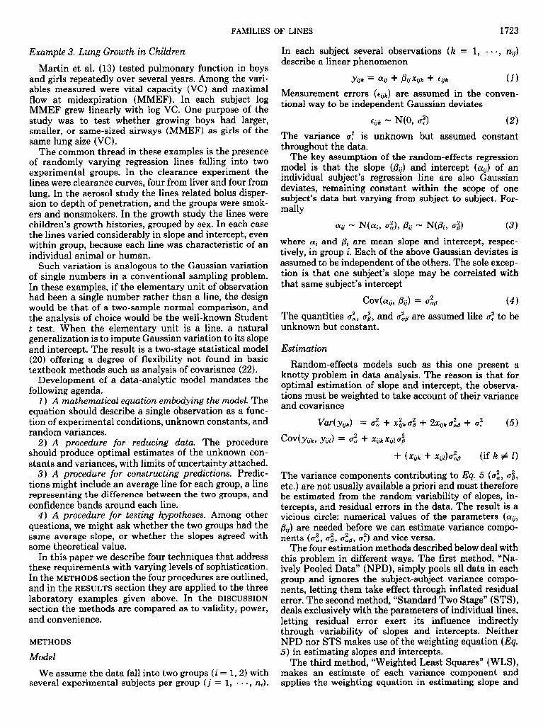
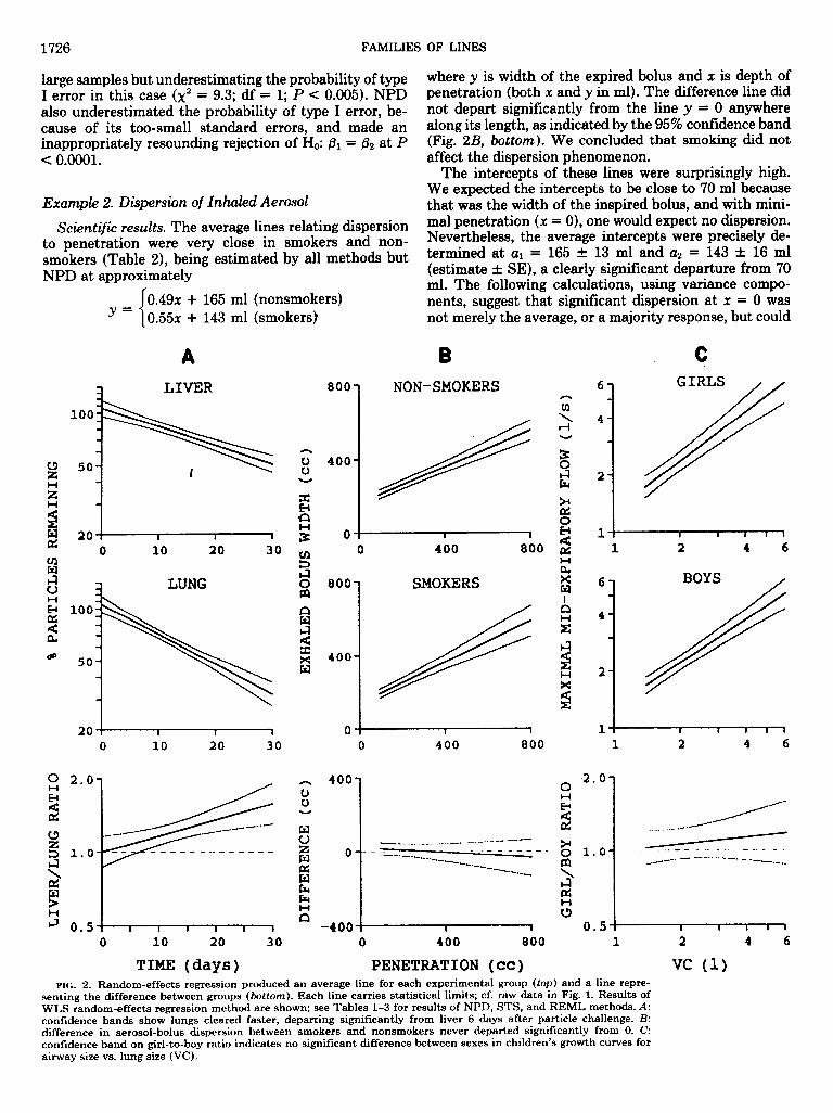
In each example we first report the scientific results: a story of clearance times, smoking effects, sex differ- ences, etc. Then we compare stories told by the four regression methods. Tables l-3 contain a listing of estimated slopes, intercepts, standard errors, variance components, P values, and computer timings. Graphical results of WLS are presented in Fig. 2. All computations were performed by SAS procedures (18). The conver- gence criterion for REML was t0.5% in each variance component.

Example 1. Clearance of Foreign Particles

Scientific results. The average particle clearance curves, as estimated by all four methods (Table l), were

approximately

log10 y = 2.03 - 0.011 t (liver) 2.03 - 0.017t (lung)

where y is iron oxide content, expressed as percent of initial level, and t (time) is in days. Thus the half time for clearance from liver was -27 days [ (loglo 2)/0.011], whereas the lungs cleared with a shorter half time, -18 days.

The purpose of the experiment was to compare the two clearance rates, i.e., to test Ho:/& = p2. All four methods found the difference between slopes to be sta- tistically significant and estimated the probability of type I error at 5% or less (P < 0.05). We concluded that & # /32; i.e., the lungs did clear faster than liver. Rat-to-rat standard deviation of the clearance slope was estimated at sg = 0.002 day-‘, or t6 days of clearance half time, by the two procedures dealing explicitly with variance components.

StatisticaL results. WLS and REML gave virtually identical parameter estimates, variance components, and P values (Table 1). REML converged in 12 iterations. STS gave the same slopes, intercepts, and standard errors but larger variance components. Estimates of rat- to-rat standard deviation of slope and intercept were inflated by -50% in STS because of the contribution of within rat residual error. NPD produced slopes and intercepts similar to those of the other methods but underestimated the standard errors because it failed to account for within-rat covariance.

In rejecting Ho: & = p2 STS sounded the appropriate level of caution, taking note of the small sample size (nl =

n2 = 4) and estimating the probability of type I error (false rejection) at 5% (F = 7.65; df = 1, 6; P < 0.05). The other methods also rejected Ho: PI = & but were inappropriately emphatic, ignoring the small number of subjects and virtually denying the possibility of type I error. WLS and REML used the x2 statistic, valid in

TABLE 1. Example 1: particle clearance from rat liver and lung

Slope, day-’

Method Liver (b, f SE) Lung (& f SE) SD (s,d Ho:81 = c92

NPD -0.0106t0.0011 -0.0172~0.0011 P< 0.0001 STS -0.0113*0.0015 -0.0173t0.0015 0.0031 P < 0.05 WLS -0.0108*0.0015 -0.0173*0.0015 0.0021 P<O.o05 REML -0.0108~0.0015 -0.0173~0.0014 0.0020 P<O.o05

Intercept, Log,, % retention

Method Liver (al f SE) Lung (h f SE) SD W I-I&al = CT2

NPD 2.025kO.018 2.025kO.018 P>O.W STS 2.029t0.023 2.025t0.023 0.045 P > 0.90 WLS 2.026kO.023 2.025kO.022 0.030 P>O.90 REML 2.026kO.022 2.025kO.022 0.028 P>O.W

Method Computer

Time, s Iterations Error SD b,) Ho:81 = 82, (rl = (r2

NPD STS WLS REML

4.4 4.5 6.9

12.3 12

0.061 P < 0.0001 0.057 P < 0.05 0.057 P < 0.0001 0.057 P< 0.0001

See text for definitions of abbreviations.

1726 FAMILIES

large samples but underestimating the probability of type I error in this case (x2 = 9.3; df = 1; P < 0.005). NPD also underestimated the probability of type I error, because of its too-small standard errors, and made an inappropriately resounding rejection of Ho: & = p2 at P c o.ooo1.

Example 2. Dispersion of Inhaled Aerosol

Scientific results. The average lines relating dispersion to penetration were very close in smokers and nonsmokers (Table 2), being estimated by all methods but NPD at approximately

0.49n + 165 ml (nonsmokers) Y= 0.55x + 143 ml (smokers)

A

OF LINES

where y is width of the expired bolus and x is depth of penetration (both x and y in ml). The difference line did not depart significantly from the line y = 0 anywhere along its length, as indicated by the 95% confidence band (Fig. 2B, bottom). We concluded that smoking did not affect the dispersion phenomenon.

The intercepts of these lines were surprisingly high. We expected the intercepts to be close to 70 ml because that was the width of the inspired bolus, and with minimal penetration (x = 0), one would expect no dispersion. Nevertheless, the average intercepts were precisely de- termined at al = 165 t 13 ml and a2 = 143 * 16 ml (estimate t SE), a clearly significant departure from 70 ml. The following calculations, using variance components, suggest that significant dispersion at x: = 0 was not merely the average, or a majority response, but could

C

3 LIVER 800

1 NON-SMOKERS

o- 0 400 800

800 1 SMOKERS

0 : 1 1 ,I- 0 400 800 1 2 4 6

0 400 800 1 2 4 6

TIME (days) PENETRATION (cc) vc (1) FIG. 2. Random-effects regression produced an average line for each experimental group (top) and a line repre-

senting the difference between groups (bottom). Each line carries statistical limits; cf. raw data in Fig. 1. Results of WLS random-effects regression method are shown; see Tables l-3 for results of NPD, STS, and REML methods. A: confidence bands show lungs cleared faster, departing significantly from liver 6 days after particle challenge. B: difference in aerosol-bolus dispersion between smokers and nonsmokers never departed significantly from 0. C: confidence band on girl-to-boy ratio indicates no significant difference between sexes in children’s growth curves for airway size vs. lung size (VC).


TABLE 2. Example 2: aerosol bolus dispersion in human airways

Slope, ml/ml

Method Nonsmokers Smokers SD

(b, f SE) (b, f SE) ($9) I-b& = 82

NPD 0.455*0.031 0.594t0.037 P < 0.005 STS 0.485kO.044 0.556t0.052 0.138 * WLS 0.486*0.044 0.554kO.052 0.130 * REML 0.486kO.044 0.554t0.053 0.131 *

Intercept, ml

Method Nonsmokers

h f SW Smokers

(a2 f SE) SD bJ

I-I&Y~ = a2

NPD 172t15 125t17 P < 0.05 STS 165k13 141k16 41 * WLS 165t13 143*15 34 * REML 165k13 143k16 36 *

Method Computer

Time, s Iterations Error SD be)

Ho:/% = 02, (rl = cT2

NPD STS WLS REML

4.9 4.8 7.7

11.5 4

61 28 28 28

P < 0.01 P > 0.40 P > 0.40 P > 0.40

See text for definitions of abbreviations. * Not tested because Ho:& = r6 241 = ac2 accepted.

be expected in virtually the entire population. Subject- to-subject standard deviation of the intercept, as estimated by WLS and REML, was approximately s, = 35 ml. A smoker with no dispersion (cuzi = 70 ml) would therefore lie z = (70 - 143)/35 = -2.09 standard devia- tions from the mean, the lower second percentile. An even more extreme figure would be obtained for nonsmokers.

Statistical results. WLS and REML results were very close to one another, REML converging in four iterations (Table 2). STS estimated oa 50% higher but agreed with WLS and REML as to parameters, standard errors, and P values in testing Ho: p1 = &,, cyl = cy2. The sample size was apparently large enough (nl = 10, n2 = 7) that WLS and REML did not noticeably underestimate the probability of type I error, agreeing with STS on P > 0.40.

NPD was badly “fooled” by the configuration of these data, lacking information on which data derived from a particular subject. The nonsmokers’ lines were parallel but vertically spread out (Fig. lB, top); NPD misinterpreted this pattern as a shallower slope. One smoker’s data lay low and to the left, another’s high and to the right (Fig. lB, bottom); NPD misinterpreted that pattern as a steeper slope. Where slope was overestimated, intercept was underestimated, and vice versa. The hypothesis of identical mean lines was rejected firmly (F = 5.10; df = 2,168; P < 0.01). This was certainly a false rejection, even though NPD estimated the probability of type I error at <l%. NPD also overestimated s, by 100% because of the unaccounted contributions of s, and so.

Example 3. Lung Growth in Adolescence

Scientific results. The mean lines for lung growth were approximately

log,, MMEF = 0.11 + 0.85 loglo VC (girls) 0.11 + 0.75 loglo VC (boys)

(Table 3). A slope different from 1 would suggest that airflow did not grow proportionally to lung volume. The four regression methods generally agreed that the boys’ mean slope was significantly Cl, but the girls’ was not. However, a direct comparison of boys with girls yielded no significant difference either between the slopes or between the whole lines (Fig. 2C). The likely truth is that airways in both boys and girls grew somewhat less than proportionally to lung volume (slope Cl), but a larger sample would be needed to demonstrate the fact in girls or to demonstrate the sex difference. The variance components produced by a random-effects analysis might provide the necessary information to construct a power curve or perform a sample-size calculation for further experiments.

Statistical results. WLS and REML yielded nearly the same estimates of parameters and variance components, REML taking 11 iterations (Table 3). The STS estimate of boys’ slope was lower than that of WLS or REML, possibly because of the influence of one anomalous subject. Male subject 220 had four data points, closely spaced in x: (VC) with a negative slope. The subject received relatively little weight in WLS or REML because of his small sample size and weak design; such information was not available to STS. NPD likewise underestimated the boys’ slope, presumably being misled as in example 2 by the considerable vertical spread of subjects’ parallel tracks (Fig. 1C).

STS responded to high variability within subjects by estimating ag twofold higher and ca ninefold higher than WLS or REML. NPD overestimated 6, twofold. Hypoth- esis tests were virtually identical by all methods except NPD. The sample size was apparently large enough (nl = 8, n2 = 15) that WLS and REML calculated the probability of type I error in agreement with STS at 30- 50%. NPD rejected Ho: ,& = p2, cyl = cy2 at P < 0.05, again overestimating statistical significance.

TABLE 3. Example 3: growth of children’s airways and parenchyma

Slope, log& MMEF per log,,-,l VC

Method Girls (b, f SE) Boys (b, f SE) SD b,,) Ho& = 82

NPD 0.863kO.124 0.700*0.083 P > 0.20 STS 0.889*0.119 0.722kO.087 0.336 * WLS 0.851*0.092 0.755-eo.068 0.142 * REML 0.858~0.091 0.752kO.066 0.129 *

Intercept, loglO l/s MMEF

Method Girls (ul f SE) BOYS (ai f SE) SD (8,) H,,xq = a2

NPD O.llSkO.057 0.114*0.041 P > 0.50 STS 0.085*0.049 O.llOkO.036 0.139 * WLS 0.114kO.036 0.115kO.028 0.016 * REML 0.114-eO.036 0.115kO.028 0.015 *

Method Computer

Time, s Iterations Emor SD (se)

Ho:& = 82, arl = a2

NPD STS WLS REML

4.5 4.6 7.1

16.1 11

0.098 0.057 0.057 0.057

P < 0.05 P > 0.40 P > 0.50 P > 0.30

See text for definitions of abbreviations. * Not tested because Ho:& = B 2,al = a2 accepted.


DISCUSSION

Regression lines, like Hamlet’s sorrows, come not single spies but in battalions. Thus besieged, many investigators know no recourse but to fire repeatedly the one weapon at hand: simple linear regression. All the while they may have the uneasy (and entirely appropriate) feeling that there must be a better way. In this paper we have described some strategies for handling the on- slaught of data.

We analyzed three disparate experiments with a common design: two groups of subjects, a regression line measured in each subject. A comprehensive methodolog- ical approach permitted us to address key questions in each study while measuring and controlling for random variability among subjects. We produced simple graphs showing the average behavior of each group and the difference between them, with confidence bands and test statistics for inference.

Most often when data in this form are brought to a consultant, the investigator has tentatively planned to combine all the data in each group, perform two simple linear regressions, and somehow compare the two lines. Confronting the troublesome “somehow” has brought him to a statistician, ostensibly to copy down the right formula. Equally troublesome, however, is a suspicion that this is not the right procedure at all, that something might be lost by pooling the data in each group. After all, why were several rats killed or several volunteers recruited in the first place? Certainly not to be treated analytically as one macrosubject. Nonetheless, the simple appeal of lumping data and applying a quick, familiar statistical test is not easily resisted. Many clients clearly hope to be told to go back and do the easy thing, namely NPD.

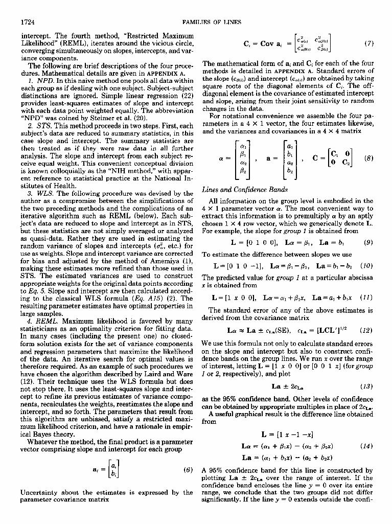
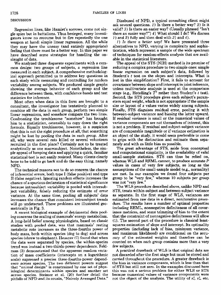
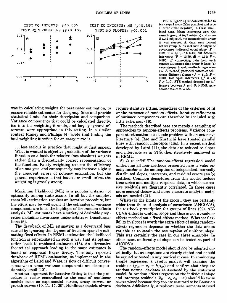
The technical reasons not to do so concern the chance of inferential errors, both type I (false positive) and type II (false negative). Ignoring random effects increases the chance of a spurious declaration of statistical significance because intrasubject variability is pooled with intersub- ject variability, falsely reducing the estimate of error variance. At the same time, pooling all subjects’ data increases the chance that consistent intrasubject trends will go undetected. These problems are illustrated geo- metrically in Fig. 3.

A recent biological example of detrimental data pooling concerns the scaling of mammals’ energy metabolism. A long-held belief among physiologists, based on classic studies with pooled data, was that mammals’ resting metabolic rate increases as the three-fourths power of body mass, both within species (dog to dog) and across species (shrew to elephant). Heusner (7) found that when the data were separated by species, the within-species trend was instead a two-thirds-power dependence. Feld- man (3) demonstrated that the apparent random variation of mass coefficients (intercepts on a logarithmic scale) expressed a precise three-fourths-power dependence across species. The two different powers suggest that “animal design” is constrained by one set of physiological determinants within species and another set across species. Steimer et al. (20) further detail the pitfalls of NPD and its cousin, “Naively Averaged Data.”

Disabused of NPD, a typical consulting client might ask several questions. 1) Is there a better way? 2) Is it valid? 3) Is there an easier way? (Usually phrased “Isn’t there an easier way?“) 4) What should I do? We discuss 1) and 2) fully and then deal with 3) and 4).

1) Is there a better way? We have presented three alternatives to NPD, varying in complexity and sophistication, which represent a sample of the wide spectrum of techniques for random-effects analysis that are available in the statistical literature.

The appeal of the STS (NIH) method is its promise of reducing a complex procedure to two simple ones: simple linear regression on each subject’s data, followed by Student’s t test on the slopes and intercepts. What is lost in this simplification? First, it fails to account for covariance between slope and intercept in joint inference, unless multivariate analysis is used at the comparison stage (e.g., Hotelling’s T2 rather than Student’s t test). Second, the STS procedure gives each subject’s parameters equal weight, which is not appropriate if the sample size or layout of x values varies widely among subjects. Finally, STS disguises residual error, pooling it with between-subject variance and biasing the latter upward. If residual variance is small or the numerical values of variance components are not themselves of interest, this is not a problem. If residual and subject-subject variance are of comparable magnitude or if variance estimation is an object of the study, it would seem preferable to come to grips with the distinction and estimate them sepa- rately and with as little bias as possible.

The great advantage of STS, aside from conceptual and computational simplicity, is the availability of valid small-sample statistics. STS can thus be relied on, whereas WLS and REML cannot, to produce accurate P values in cases of very few subjects, so long as the assumptions of the small-sample model (e.g., normality) are met. In our examples we found four subjects per group to be “very few,” whereas 10 subjects per group was not “very few.”

The WLS procedure described above, unlike NPD and STS, treats within-subject and between-subject variance as separate. In the first stage of WLS, variances are estimated from raw data in a direct, noniterative procedure. The results have a number of optimal properties including REML, nonnegative definiteness of all covariance matrices, and some trimming of bias to the extent that the constraint of nonnegative definiteness will allow (1). The second part of the procedure is classical least- squares estimation of slope and intercept. Its optimality properties (including lack of bias, minimum variance, and maximum likelihood) are conditional on the accu- racy of the estimated weights and therefore can be counted on when each group contains more than a very few subjects.

A practical drawback of WLS is that original data are not discarded after the first stage but must be stored and carried throughout the procedure. A greater drawback is the bias in variance components, which is less than that of STS but still not zero. In the examples discussed here this was not a serious problem for either WLS or STS because numerical values of variance components were not the object of the analysis. The utility of ST, st, etc.

TEST EQ INTCPTS: ~(0.005 TEST EQ INTCPTS: NS (p>O.lO) TEST EQ SLOPES: NS (p>O.lO) TEST EQ SLOPES: p<O.OOl

0.3

0.2

sr

0.1

0.0

l

l

I I I I I I I1 1

-4 0 4

x


0.3

0.2

0.1

0.0 -4

I 1 I I I I 1 11

was in calculating weights for parameter estimation, to ensure reliable estimates for the group lines and provide statistical limits for their description and comparison. Variance components that could be calculated directly, fed into the weighting formula, and largely ignored af- terward were appropriate in this setting. In a similar context Finney and Phillips (4) wrote that finding the best weighting function for an assay curve is

. less serious in practice that might at first appear. What is wanted is objective graduation of the variance function as a basis for relative (not absolute) weights rather than a theoretically correct representation of the function. Faulty weighting reduces the efficiency of an analysis, and consequently may increase slightly the apparent errors of potency estimation, but the general experience is that losses are small unless the weighting is grossly wrong.

Maximum likelihood (ML) is a popular criterion of optimality among statisticians. In all but the simplest cases ML estimation requires an iterative procedure, but the effort may be well spent if the estimates of variance components are to be the highlight of the random-effects analysis. ML estimates have a variety of desirable properties including invariance under arbitrary transforma- tions (6).

The drawback of ML estimation is a downward bias caused by ignoring the degrees of freedom spent in estimating fixed effects. In REML estimation the likelihood function is reformulated in such a way that its optimi- zation leads to unbiased estimates (15). An alternative theoretical approach leading to the same estimates is based on empirical Bayes theory. The only reported drawback of REML estimation, as implemented in the algorithm of Laird and Ware, is slow or difficult conver- gence when some variance components are dispropor- tionately small (12).

Another argument for iterative fitting is that the procedure is easily generalized to the case of nonlinear models such as exponential curves, assay curves, or growth curves (10, 11, 17, 20). Nonlinear models always

0 4

X

FIG. 3. Ignoring random effects led to both type I error (false positive) and type II error (false negative) in these simu- lated data. Mean intercepts were the same in group A (0; 2 subjects) and group B (A; 2 subjects), but mean slope in group B was steeper. A: data were pooled within group (NPD method). Analysis of covariance indicated equal slope (F = 2.82; df = 1,15, P > 0.10) but different intercepts (F = 12.70, df = 1,15; P < 0.005). B: connecting data from each subject illustrates that group B lines (A) were steeper. Random-effects regression (WLS method) provided correct conclu- sions: different slopes (x2 = 11.3; P < 0.001) but equal intercepts (x2 = 2.6; P > 0.10). STS method detected no difference between A and B; REML gave similar result to WLS.

require iterative fitting, regardless of the criterion of fit or the presence of random effects. Iterative refinement of variance components can therefore be included with little extra cost (16).

The methods described here are merely a sampling of approaches to random-effects problems. Variance component estimation is a classic problem with an extensive literature (6). Rae and Kuranchi have treated parallel lines with random intercepts (16a). In a recent method developed by Laird (ll), the data are reduced to slopes and intercepts as in STS, then iteratively improved as in REML.

2) Is it ualid? The random-effects regression model underlying all four methods presented here is valid ex- actly insofar as the assumption of independent, normally distributed slopes, intercepts, and residual errors can be justified. Common departures from this model include time series and multiple-response data, in which succes- sive residuals are flagrantly correlated. In those cases more general theory and more elaborate analytic methods are needed (21).

Whatever the limits of the model, they are certainly wider than those of analysis of covariance (ANCOVA), the textbook prescription for groups of lines (22). AN- COVA enforces uniform slope and thus is not a random- effects method but a fixed-effects method. Whether flexibility in slopes is worth the extra effort of using random- effects regression depends on whether the data are so variable as to strain the assumption of uniform slope. This was certainly the case in our three examples. In other cases uniformity of slope can be tested as part of ANCOVA.

The random-effects model should not be adopted un- critically. Its assumptions are clearly stated and should be argued or tested in any particular case. In conducting simple regression, a careful analyst will examine the residuals (yijh - aG - bijXijJ and confirm that they are random normal deviates as assumed by the statistical model. In random-effects regression the individual slope and intercept residuals (bG - bi, au - ai) should likewise be examined because they too are assumed to be Gaussian deviates. Additionally, if replicate measurements at fixed


xgk are available, the assumption of intrasubject linearity variation, and one for residual variation

can be tested, just as in simple regression (22). 3) Is there an easier way? Certainly there is an easier

way: lump all the data in each group, do simple linear (A4)

regression, and never, never consult a statistician. Many investigators take this approach. Fortunately, others

The random vectors are assumed to be drawn from a multivar-

take statistical analysis seriously and understand that it iate normal distribution

can deal with scientifically pertinent questions of random [ I

aij-ati

variability on the level of subjects as well as residuals. ,8ij-8i

- N(0, D), D = 2 5 9 eii- N(0, 21) [ I

(A5) 4 B

4) VVIz& should I do? The author believes the STS method represents the minimum required to deal with where I is the identity matrix. random effects in this common design. WLS and REML add significant quanta of analytic power and are worth the extra intellectual and computational effort for a

step za. Estimation Of~~iv~~ Lines

scientist concerned with doing justice to hard-earned Simple linear regression provides individual intercepts and data. slopes

APPENDIX A

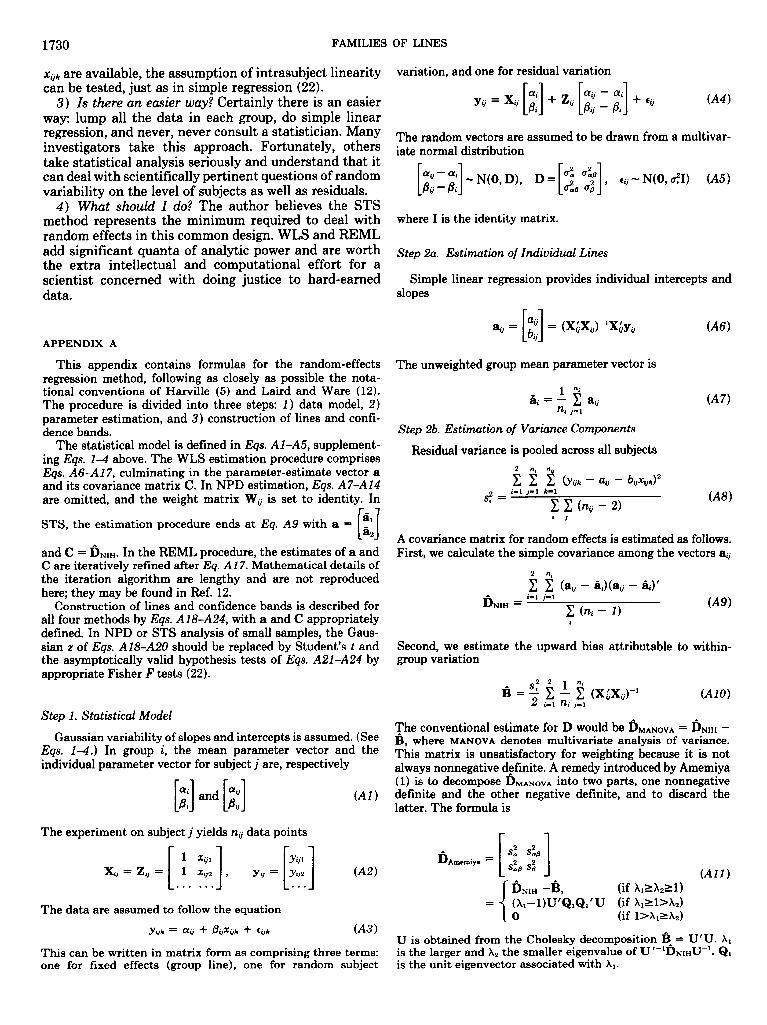
This appendix contains formulas for the random-effects regression method, following as closely as possible the notational conventions of Harville (5) and Laird and Ware (12).

The procedure is divided into three steps: 1) data model, 2) parameter estimation, and 3) construction of lines and confidence bands.

The statistical model is defined in Eqs. Al-A5, supplement- ing Eqs. 1-4 above. The WLS estimation procedure comprises Eqs. A6-A17, culminating in the parameter-estimate vector a and its covariance matrix C. In NPD estimation, Eqs. A7-Al4 are omitted, and the weight matrix Wti is set to identity. In

and C = DNIH. In the REML procedure, the estimates of a and C are iteratively refined after Eq. Al 7. Mathematical details of the iteration algorithm are lengthy and are not reproduced here; they may be found in Ref. 12.

Construction of lines and confidence bands is described for all four methods by Eqs. Al&A24, with a and C appropriately defined. In NPD or STS analysis of small samples, the Gaus- sian z of .Eqs. Al&A20 should be replaced by Student’s t and the asymptotically valid hypothesis tests of Eqs. A21-A24 by appropriate Fisher F tests (22).

Step 1. Statistical Model

Gaussian variability of slopes and intercepts is assumed. (See Eqs. l-4.) In group i, the mean parameter vector and the individual parameter vector for subject i are, respectively

ri ri

8ij = = (x;x,)-'x;y, (A@

The unweighted group mean parameter vector is

1 "i

Qi =- x

ni j-1 aii

Step 2b. Estimation of Variance Components

Residual variance is pooled across all subjects

i j

A covariance matrix for random effects is estimated as follows. First, we calculate the simple covariance among the vectors aii

W)

VW

6 i-l j-l

NIH =

c,< - 1) W)

ni

Second, we estimate the upward bias attributable to within- group variation

B = 2 i 1 5 (Xg&....-1 i-l ni j-l

(AlO)

The conventional estimate for D would be &NOVA = DNiH - & where MANOVA denotes multivariate analysis of variance. This matrix is unsatisfactory for weighting because it is not always nonnegative d$inite. A remedy introduced by Amemiya (1) is to decompose D MANovA into two parts, one nonnegative

(Al) definite and the other latter. The formula is

negative definite, and to discard the

The experiment on subject i yields n,-,- data points r

(All) L . . . . . . J L-J

The data are assumed to follow the equation

6 4, NIH (if X,&>l)

(Xl-l)U’Q,Q,‘U (if X1d>X2)

0 (if l>X1&)

Yijk = a@ + &jxtik + fijk (A3 U is obtained from the Cholesky decomposition fi = U’U. X1

This can be written in matrix form as comprising three terms: is the larger and X2 the smaller eigenvalue of UI-lDN&-‘. Q1 one for fixed effects (group line), one for random subject is the unit eigenvector associated with X1.


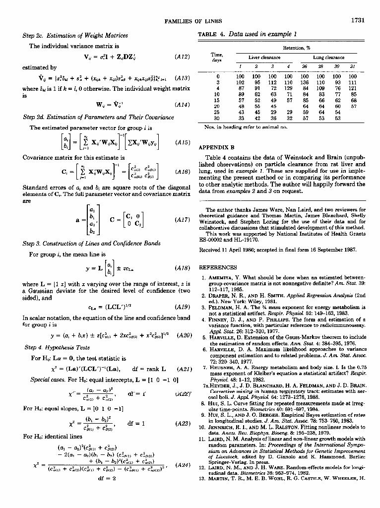
Step 2~. Estimation of Weight Matrices

The individual variance matrix is

v&-j = d1 + &DZ;

estimated by

TABLE 4. Data used in example 1

Retention, %

(Am Time, &YS

Liver clearance Lung clearance

1 2 3 4 26 28 30 31

Qti = (Sfa&J + Sz + (Xijk + Xijl)SXfl + XijkXijdS$)$F 1-1 W3) 0 loo 100 100 100 100 100 loo loo 3 102 95 112 110 136 110 93 111

where bkl is 1 if k = 1,O otherwise. The individual weight matrix 4 87 91 72 129 84 109 76 121 is 10 89 62 63 71 84 83 77 85

wti = $?,I (AM 15 57 52 49 57 85 66 62 68 20 48 55 45 64 64 60 57 25 43 45 29 29 59 64 54

Step 2d. Estimation of Parameters and Their Covariance 30 33 42 36 32 57 53 53

The estimated parameter vector for group i is Nos. in heading refer to animal no.

Covariance matrix for this estimate is

Standard errors of ai and bi are square roots of the diagonal elements of Ci. The full parameter vector and covariance matrix are

r i a1 L -

Step 3. Construction of Lines and Confidence Bands

For group i, the mean line is

(A17)

Y = L 11 ii t ZCL, (Am i

APPENDIXB

Table 4 contains the data of Weinstock and Brain (unpublished observations) on particle clearance from rat liver and lung, used in example 1. These are supplied for use in imple- menting the present method or in comparing its performance to other analytic methods. The author will happily forward the data from examples 2 and 3 on request.

The author thanks James Ware, Nan Laird, and two reviewers for theoretical guidance and Thomas Martin, James Blanchard, Shelly Weinstock, and Stephen Loring for the use of their data and for collaborative discussions that stimulated development of this method.

This work was supported by National Institutes of Health Grants ES-00002 and HL-19170.

Received 11 April 1986; accepted in final form 16 September 1987.

REFERENCES L -A

1.

where L = [l x] with x varying over the range of interest, z is a Gaussian deviate for the desired level of confidence (two sided), and 2.

Ch = (LcL’y2 (A19) 3.

In scalar notation, the equation of the line and confidence band 4 . for group i is

y = (ai + biX) t Z[Ci(i) + 2XC&(i) + X2C$(i)]1’2 ww 5

Step 4. Hypothesis Tests 6.

For Ho: La = 0, the test statistic is

x2 = (La)‘(LCL’)-‘(La), df = rank L (A21) 7.

Special cases. For Ho: equal intercepts, L = [ 1 0 -1 01 -

AMEMIYA, Y. What should be done when an estimated between- group covariance matrix is not nonnegative definite? Am. Stat. 39: 112-117,1985. DRAPER, N. R., AND H. SMITH. Applied Regression Analysis (2nd ed.). New York: Wiley, 1981. FELDMAN, H. A. The 9/r mass exponent for energy metabolism is not a statistical artifact. Respir. Physiol. 52: 149-163, 1983. FINNEY, D. J., AND P. PHILLIPS. The form and estimation of a variance function, with particular reference to radioimmunoassay. Appl. Stat. 26: 312-320,1977. HARVILLE, D. Extension of the Gauss-Markov theorem to include the estimation of random effects. Ann. Stat. 4: 384-395,1976. HARVILLE, D. A. Maximum likelihood approaches to variance component estimation and to related problems. J. Am. Stat. Assoc. 72: 320-340,1977. HEUSNER, A. A. Energy metabolism and body size. I. Is the 0.75 mass exponent of Kleiber’s equation a statistical artifact? Respir. Physid. 48: l-12,1982.

7a.HEYDER, J., J. D. BLANCHARD, H. A. FELDMAN, AND J. D. BRAIN.

c:(l) + C(2) -

8. For Ho: equal slopes, L = [O 1 0 -11

(b b) 2

x2= l - 2 G(l) + 42) ’

df=l

9.

(AM 10 .

For Ho: identical lines

(al - a2)2(4(1) + 42))

- %a1 - a2)(bl - bd (&l) + c$2J

11.

a=2 13.

Corrective mixing in human respiratory tract: estimates with aerosol boli. J. Appl. Physiol. 64: 1273-1278,1988. HUI, S. L. Curve fitting for repeated measurements made at irreg- ular time-points. Biometrics 40: 691-697,19&L HUI, S. L., AND J. 0. BERCER. Empirical Bayes estimation of rates in longitudinal studies. J. Am. Stat. Assoc. 78: 753-760,1983. JENNRICH, R. I., AND M. L. RALSTON. Fitting nonlinear models to data. Annu. Rev. Biophys. Biueng. 8: 195-238,1979. LAIRD, N. M. Analysis of linear and non-linear growth models with random parameters. In: Proceedings of the International Sympo- sium on Advances in Statistical Methods for Genetic Improvement of Livestock, edited by D. Gianolo and K. Hammond. Berlin: Springer-Verlag. In press. LAIRD, N. M., AND J. H. WARE. Random-effects models for longitudinal data. Biometrics 38: 963-974,1982. MARTIN, T. R., M. E. B. WOHL, R. G. CASTILE, W. WHEELER, H.


A. FELDMAN, AND J. MEAD. Longitudinal analysis of airflow and lung volume in children (Abstract). Am. Rev. Respir. Dis. 131: A324,1985.

14. MORRISON, D. F. Multivariate Statistical Methods (2nd ed.). New York: McGraw-Hill, 1976.

15. PAITERSON, H. D., AND R. THOMPSON. Recovery of interblock information when block sizes are unequal. Bimnetriku 58: 545-554, 1971.

16. RACINE-POON, A. A Bayesian approach to nonlinear random effects models. Biometrics 41: 1015-1023,1985.

16a.RA0, P. S. R. S., AND P. KURANCHIE. Variance components of the linear regression model with a random intercept. Commun. Stat. In press.

17. RODBARD, D., R. H. LENOX, H. L. WRAY, AND D. RAMSETH.

Statistical characterization of the random errors in the radioimmunoassay dose-response variable. Clin. Chem. 22: 350-358, 1976.

18. SAS INSTITUTE, INC. SAS User’s Guide: Basics. Cary, NC: SAS Institute, 1982, p. 431-476.

19. SEARLE, S. R. Linear Models. New York: Wiley, 1971. 20. STEIMER, J.-L., A. MALLET, AND F. MENTR~ Estimating interin-

dividual pharmacokinetic variability. In: Variability in Drug Ther- apy, edited by M. Rowland, L. B. Sheiner, and J.-L. Steimer. New York: Raven, 1985, p. 65-109.

21. WARE, J. H. Linear models for the analysis of longitudinal studies. Am. Stat. 39: 95-101,1985.

22. ZAR, J. H. Biostatistical Analysis (2nd ed.). Englewood Cliffs, NJ: Prentice-Hall, 1984.

families of lines: random effects in linear regression

Documents