family trajectories and health. a life course perspective

Family trajectories and health. A life courseperspective

Nicola Barban

DONDENA “Carlo F. Dondena” Centre for Research on Social Dynamics,

Universita Bocconi, Milan, Italy

[email protected]

Draft version.

Abstract

In this paper, I investigate the role of family trajectory, i.e. the whole sequence offamily events, during the life course of early adults in shaping their health outcomes.I jointly consider union formation and childbearing, since the two life domains arehighly connected and their intersections may have an effect on health outcomes.Data come from Wave I and Wave IV of the National Longitudinal Study of Ado-lescent Health (Add Health). The paper is divided in two parts. First, I focus ontransitions and investigate if changes in timing (when events happen), quantum(what and how many transitions) and sequencing (in what order), have an effect onthe health of young women. In the second part, I classify life course trajectories intosix groups representing different ideal-types of family trajectories and I explore theassociation of these trajectories with health outcomes. Results suggest that familytrajectories play an important role on different health outcomes. Controlling for se-lection and background characteristics, precocious and “non-normative” transitionsare associated with lower self-reported health and higher propensity of smoking anddrinking.

1 Introduction

During the last decade, there has been an increasing interest in the relationship between

marital status and health, (see e.g. Schoenborn, 2004; Waite and Bachrach, 2000; Wood

et al., 2007; Koball et al., 2010). This is partially motivated by the recent changes in

family behavior that have occurred in the United States and many other Western coun-

tries, i.e. increase in cohabitation, delay in marriage and rise of non marital childbearing

(Cherlin, 2005; Schoen et al., 2007). Studies on the United States highlight the positive

association between marriage and a various range of health outcomes for both men and

women. Married adults are less likely to die in any given period than the unmarried

(Lillard and Waite, 1993; Dupre et al., 2009), they also appear to have better mental

1

health than their counterparts (Lamb et al., 2003; Horwitz and White, 1998; Soons and

Kalmijn, 2009; Meadows, 2009) and they are less likely to engage in unhealthy behaviors

(Duncan et al., 2006).

Most studies examine health differences by marital status in order to identify the

causal effect of marriage. Generally, they compare health outcomes of married men and

women versus unmarried (or cohabiting) people or they examine the effect of changes in

marital status across life course (Nock, 1981). Only a limited number of studies adopts

a complete life course perspective. The life course paradigm assumes that individuals,

as human agents, build their future on the basis of the constraints and opportunities

experienced in the past (Elder, 1994). The process is iterative and cumulative, since initial

advantages or disadvantages often are amplified with time (Giele and Elder, 1998). Life

courses are embedded in different time and location and are affected by the social context

in which individuals live. In addition, different life domains are strongly interdependent.

Elder (1985) observes that a trajectory can also be envisioned as a sequence of tran-

sitions that are enacted over time. A transition is a discrete life change or event within

a trajectory (e.g., from single to married), whereas a trajectory is a sequence of linked

states within a conceptually defined range of behavior or experience. Transitions are often

accompanied by socially shared ceremonies and rituals, such as a graduation or a wed-

ding ceremony, whereas a trajectory is a long-term pathway, with age-graded patterns of

development in major social institutions such as education or family. In this way, the life

course perspective emphasizes the ways in which transitions, pathways, and trajectories

are socially organized. Moreover, transitions typically result in a change in status, social

identity, and role involvement. Trajectories, however, are long-term patterns of stability

and change and can include multiple transitions. Using longitudinal or retrospective data,

family trajectories can be described by the complete sequence over time of union status,

childbearing and eventually work status. Life course scholars stress the importance of the

long term effects of trajectories (Soons et al., 2009), together with other characteristics

of life history. Rather than investigating the contemporaneous association between mar-

ital status and wellbeing, life course analysis looks at the entire development of family

history, i.e. the whole trajectory. Under this perspective, characteristics such as type,

number and duration of unions, or the order of events may have an effect on later health

outcomes (Peters and Liefbroer, 1997).

In this paper, I investigate the role of family trajectory, i.e. the whole sequence of

family events, during the life course of early adults in shaping their health outcomes. I

jointly consider union formation and childbearing, since the two life domains are highly

connected and their intersections may have an effect on health outcomes. This paper is

divided in two parts. First, I focus on transitions and investigate if changes in timing

2

(when events happen), quantum (what and how many transitions) and sequencing (in

what order) (Billari et al., 2006; Billari, 2005), have an effect on the health of young

women. In the second part, I classify life course trajectories into six groups representing

different ideal-types of family trajectories and I explore the association of these trajecto-

ries with health outcomes.

2 Theoretical and empirical background

According to the life course health development (LCHD) model, health is the result of

a continuous process that develops over an individual’s lifetime (Halfon and Hochstein,

2002). In the LCHD model, health is a consequence of multiple factors operating in nested

genetic, biological, behavioral, social, and economic contexts. These contexts change as a

person develops. Therefore, health is seen as an adaptive process, composed by multiple

transactions between the contexts mentioned above (e.g., genetic, social) and the biobe-

havioral regulatory systems (e.g., neurological, endocrine) that define human functions

(Halfon and Hochstein, 2002). In other words, health is not a static phenomenon. It

develops over time and changes as a function of experience. The LCHD model suggests

that a person’s health takes on a trajectory that results from the cumulative influence of

multiple risk and protective factors during life course. Health, in turn, is a multidimen-

sional concept that encompasses a large array of measures, including behavioral, physical,

and emotional outcomes.

The association between family transitions and health is well documented. Changes in

the family structure may affect health in several ways. In particular, Wood et al. (2007)

distinguish five different health dimensions: health behaviors, mental health, physical

health and longevity, health care access and use, intergenerational health effects. In this

paper, I will only consider the first three dimensions. Using a sample of young women in

the United States, I study the consequences of family trajectories on self-reported health,

depression, drinking and smoking behaviors.

A large number of works demonstrates that married people are healthier, happier and

less likely to engage in health threatening behaviors (for a review see Wood et al., 2007;

Schoenborn, 2004). These potential benefits of marriage have influenced, at least in part,

several US governmental initiatives in recent years that encourage and support marriage

(Lichter et al., 2003; Acs, 2007). Consequently, this led to a debate on the effectiveness of

pro-marriage policies among the scientific community, (McLanahan, 2007; Amato, 2007;

Nock, 2005).

In the literature, the benefits associated with marriage are generally called the “pro-

tection effects” of marriage (Waldron et al., 1996). In their review, Musick and Bumpass

(2006) suggest four possible explanations: institutionalization, social roles, social support

3

and commitment. Marriage is an institution where spouses have defined social roles both

inside and outside the household (Gove, 1972; Ferree, 1990). Moreover, marriage is a

source of social support. Spouses provide intimacy, companionship and daily interaction.

At the same time, married people are connected to a larger network (e.g. friends, kin).

This enlarges the social capital from which spouses can draw on in case of need. Last, the

public nature of marriage strengthens commitment and facilitates joint long-term invest-

ments, including financial, role specialization and time spent in the care of young children.

Commitment strengthens bonds between partners and serves as a barrier to exit. It is not

clear, however, if these benefits are unique to marriage or whether they can be extended

to other intimate relationship, particularly cohabitation. Evidences are mixed: Wu and

Hart (2002) find no health effects of entering into marriage or cohabitation in Canada.

Horwitz and White (1998) find differences in happiness, but no disadvantages in terms

of depression. Musick and Bumpass (2006) examine several dimensions of wellbeing in-

cluding psychological health, social ties and relationship quality and they do not find

significative differences between married and cohabiters. In a comparative research using

data from 30 european countries, Soons and Kalmijn (2009) find that the cohabitation

gap (with respect to marriage) in wellbeing is associated with the degree of acceptance

of non-marital unions in the society.

Although there is an extensive literature on the association between marital status

and health outcomes, a number of issues motivates a life course perspective. First, the

association between marriage and wellbeing may reflect preexisting conditions. Healthy

individuals may be more likely to possess certain characteristics, such as higher earnings,

emotional health, and physical attractiveness, that make them more desirable marriage

partners than those in poor health. In contrast, those with poor mental or physical

health may lack the energy and well-being necessary to find a spouse or a partner. Most

of the studies take into account selection issues using longitudinal data and controlling

for the “individual effect”. This is done generally using “fixed effect models” or “lagged

dependent variable” regression, where the researcher can take in consideration selection

controlling for previous outcomes. Although these statistical models take into account

selection, they generally do not solve the problem of reverse causation. In some situa-

tions, health status may be the cause, rather than the effect of family transitions. For

instance, once married, those who are less healthy may be less able to communicate and

to participate in activities with their partner, or may have difficulties to contribute fi-

nancially to the household, all of which may increase the likelihood of divorce.

Second, when data on marital status are collected in a longitudinal survey, we often

ignore what happens between the time periods that are taken in consideration. Cohab-

itation and marriage are not mutually exclusive. In the United States, about half of

4

young adults live with a partner before marrying. For some people, cohabitation is a

prelude to marriage or a trial marriage. For others, a series of cohabiting relationships

may be a long-term substitute for marriage (Cherlin, 2005). Although cohabitation has

become common in the United States, it rarely lasts long. About half of cohabitation

relationships end through marriage or a breakup within a year (Seltzer, 2004; Bumpass

and Lu, 2000). If we consider only the change in marital status between the two waves of

a longitudinal survey, we may ignore possible variations occurring in between. This may

lead to considerable bias if the time between two data collection is sufficiently large. For

instance, we may not distinguish between an individual married for the first time and an-

other one who remarried after a separation. Also, since many married people experience

cohabitation, it may be difficult to separate the causal effect of marriage. Does marriage

have a different effect if it is preceded by cohabitation? In this case, does the time of

exposure to premarital cohabitation matter?

Third, the majority of studies focus on union status without taking into consideration

the link with other life domains. Union status is clearly connected with other events

that happen during the life course. Having a child, leaving parental home, finishing

school, starting to work are strictly connected with the probability to enter (or exit) a

union. For example, a couple may decide to marry because of an unplanned pregnancy,

or they can decide to postpone marriage until she/he reaches economic independence.

Since different domains are strictly interlaced, it may be difficult to identify the effect of

a single event, such as marriage or entering a cohabitation. Other variables may confound

the effect of family transitions. There may be, in fact, interactions between family events

and background characteristics such as race, socio-economic status or social context.

For instance, Harris et al. (2010) observed that early marriage by young adults does

not have a protective effect for African Americans as observed for whites. Moreover,

numerous studies show that individuals who marry at young age have higher risk of

marital dissolution (Martin and Bumpass, 1989; Bumpass et al., 1991; Lehrer, 1988;

Teachman, 2002).

Numerous studies try to investigate the causal link between divorce and premarital

unions. Marital dissolution is higher among couple who experienced cohabitation. This

negative effect is partially explained by self-selection (Lillard et al., 1995) and it is asso-

ciated with the degree of acceptance of non-marital unions in the society (Liefbroer and

Dourleijn, 2006). Moreover, Mazzuco (2009) found that the cohabitation length effect on

duration of marriage is time varying, being close to zero for the first 2-3 years of cohabi-

tation and rising considerably in the following years. Also low socioeconomic status may

constitute a barrier to enter marriage (Edin and Reed, 2005; Schoen et al., 2009) and

lead to other family transitions.

Last, standard analyses do not consider variations in timing, quantum and sequenc-

5

ing of life course trajectories. It is not clear, in fact, how changes in the structure of

trajectories affect health outcomes later in life. Most researches, in fact, do not take

into account when transitions occurs (timing), how many (quantum) and in what order

they happen (sequencing). Transitions that occur in different periods of life may have a

different effect on wellbeing. For instance, age at first union may be associated to health

outcomes. Marriages at age 18 and 30 are qualitatively very different, indeed. At the

same time, the sequence of events is relevant on the study of family life course. Does

marriage have the same effect on health if it is preceded by the birth of a child? Evidence

shows that unmarried mothers fare worse in the marriage market, because they have

greater chances of partnering with poorly educated and unemployed men (Ermisch and

Pevalin, 2005). However, it is not clear if this increases the risk of having worse health

outcomes. Last, trajectories may be very different in terms of complexity. Some individ-

uals may experience a large number of transitions while others may not. Does stability

in family trajectories affect health outcomes? Does the number of transitions matter?

Some scholars argued that the overall structure of the life course has changed in profound

ways, becoming “de-standardized,” “de-institutionalized,” and increasingly “individual-

ized” (Macmillan, 2005; Shanahan, 2000; Elzinga and Liefbroer, 2007). It is not clear,

however, what are the consequences of a de-standardization of family life course.

From a life course perspective, health outcomes are the result of the cumulative in-

fluence of multiple risks and protective factors experienced during the life course. For

this reason the association between health and family formation should be expressed as

an iterative process where health and family trajectories are mutually influenced. Un-

der this perspective, it is necessary to take into account the whole trajectory in order

to study the effects on health outcomes. The discussion above shows how difficult it

may be to assess precise causal effects of family transition, unless the researcher relies on

very strong assumptions. On the other hand, taking the whole trajectory as an input in

statistical analysis is not straightforward (George, 2009). In this study, I use sequence

analysis techniques to capture characteristics of the family trajectory such as complex-

ity, sequencing and timing. Then, using Optimal Matching (Abbott and Tsay, 2000),

I derived from data typical pathways of family formation using clustering techniques.

Rather than identifying a causal effect of single family transitions, the aim of this paper

is to explore associations between health outcomes and typologies of family trajectories.

It may be possible, in fact, that certain typologies of family formation are associated

with low health outcomes. This is relevant from a policy point of view. The study of

family trajectories may highlight disadvantaged situations and it may permit to design

appropriate interventions.

6

3 Contribution of the current study

The aim of this study is to explore the association between wellbeing and family tra-

jectories from a life course perspective. In particular, I am interested in analyzing if

there exists particular family trajectories associated with reduction in health status. To

evaluate wellbeing I focus on the analysis of four different health outcomes: Self reported

health, depression and risky behaviors (heavy drinking and smoking). I restrict the anal-

ysis to young women in age 30-33. I focused on young women for two reasons. First, the

timing of family formation events tends to be earlier for women than for men. For exam-

ple, the median age at first marriage in US is about 25 for women compared to 27 for men

(Cherlin, 2004). Given the relatively young age of the sample I use, more women than

men would have experienced family formation transitions. Second, becoming a parent is

a central variable in this analysis, and men’s reports of childbearing are less reliable than

those of women. Indeed, one third to one half of men misreport non-marital births and

births within previous marriages (Amato et al., 2008; Rendall et al., 1999).

A trajectory is defined as the monthly sequence of family states. The state-space is

defined as follows. For every woman in the sample, I collect information about marriage

and cohabiting relations. Moreover, I gather information about the age (in months) at

first birth. The combination of union status with parenthood gives these six states: Single;

Single Parent; Cohabiting; Cohabiting Parent; Married and Married Parent. Union states

are reversible since from cohabitation it is possible to go into marriage or to return to

single after a family disruption. Parenthood instead, is not reversible, i.e. from Single

Parent a woman can only go to Cohabiting Parent or Married parent. The six states

configuration follows the work by Schoen et al. (2007), where the authors examined early

family transitions using a multi-state life table framework. The monthly detail permits

to address in a precise way the order of transitions and to reduce the bias due to time

interval. Differently from Amato et al. (2008), I take into consideration only family

events (i.e. unions and childbearing) to focus on the relationship between health and

family trajectories.

Following a life course perspective, I intend to analyze the association between differ-

ent types of family trajectories and self-reported health, depression symptoms and risky

behaviors. In the first part of the empirical analysis, I focus separately on variations

in timing, quantum and sequencing of family transitions. In the second part, I classify

family trajectories in homogeneous groups sharing similar characteristics. The effect of

selection and confounding variables is considered using appropriate statistical models. In

reference to variation of timing quantum and sequences, I specify three different research

hypotheses.

H1: Women who have earlier transitions have lower health outcomes. (Timing hypothe-

7

sis)

I hypothesize that women who postpone family formation are more likely to invest in

education and accumulate human capital. Young mothers or young women that enter an

union have, in fact, less time to accumulate resources that contribute avoiding poor health

and depression (Miech and Shanahan, 2000). Higher education also prevent women from

engaging in behaviors that can damage their health. Furthermore, low educated women

are more likely to match low educated men with higher probability of being unemployed

and with lower income. Last, early marriage and early motherhood are associated with

a higher probability of marital disruption that, in turn, is associated with major stress

(Ermisch and Pevalin, 2005; O’Connell and Rogers, 1984).

H2: Women with “disordered” trajectories have lower health outcomes. (Quantum hy-

pothesis)

Women who experience a large number of transitions are more likely to have less stable

unions and may experience more traumas that can be dangerous for health development.

The concept of “disorder” has been introduced for the first time by Rindfuss et al. (1987)

in the study of transition to adulthood and parenthood. Individuals have expectations

in terms of the role they assume in the society. A “disordered” life course may reflect

difficulties to achieve the desired social role and fulfill the expectations. Also the lack of

stability in family roles may be associated with more stress and less support from others.

The “disorder” of life course is evaluated with a series of measures indicating the stability

of the trajectory.

H3: Women who have more non-normative transitions experience lower health outcomes.

(Order hypothesis)

Family transitions are not qualitatively equivalent. I expect that family transitions that

are recognized by the society as “normative” do not have negative effect on health. On the

contrary, I expect that “non-normative” transitions are associated with lower outcomes.

Individuals have expectations about the order of life-course events, even if sanctions are

not applied. In fact, many sociological theories build in an expected sequencing of events

in the transition to family. For example, first marriage is still sometimes equated with

the beginning of exposure to the risk of parenthood. The variable ordering of events in

the life course is a contingency of some importance in the life cycle (Hogan, 1978).

In the second part of the empirical analysis, I focus on family pathways. Since the pos-

sible combinations of family trajectories are enormous, I derive from data homogeneous

clusters of trajectories. The resulting typologies of family pathways describe simultane-

ously different combination of timing, quantum, and sequencing. In analogy with Amato

8

et al. (2008), I describe family formation using typical patterns of formation derived by

empirical observations. The advantage of using classes is to reduce the (almost) unlimited

number of combinations to a manageable number of groups that can be easily described.

Differently form other studies (e.g. Amato et al., 2008), I am not interested in the pre-

cursors of different family pathways, but rather the consequences. Studying the health

outcome of family typologies may help highlighting eventual disadvantages by subgroups

of population.

4 Data and methods

4.1 Sample

The data I use come from Waves I and IV of the National Longitudinal Study of Adoles-

cent Health (Add Health). Add Health is a longitudinal sample, nationally representative

of US adolescents who were in grades 7 through 12 in 1994-5. In the first wave, data

were collected through in-home interviews with the adolescent participants and one of

their parents. Typically, the parent interview was completed by the biological mother.

Adolescents were interviewed again in a second wave one year later in 1996, again in a

third wave collected in 2001-2002 and finally in a forth wave in 2008-2009. At the time

of Wave IV, respondents ranged in age from 26 to 33 years. Since the goal of this study

is to explore the implications of early life course trajectories, the sample is restricted to

women who are 30 or older at Wave IV. Of this sample (n = 2,358), Wave IV weights are

missing for 101 women. After dropping these cases, the final sample size is 2,259. At the

time of the Wave IV data collection, 27% of women in the sample were 30 years of age,

54% were 31 years of age, and 19% were 32 years of age. Using retrospective questions

from wave IV, I reconstructed the family biographies of women from age 15 to their age

at wave IV.

Health outcomes

I created the following indicators to analyze different aspects of health status, with mea-

sures available both at Wave I and at Wave IV. Measures are expressed in a continuous

scale, and indicate physical, mental health, drinking and smoking behaviors.

Self-reported Health

Status of current health was assessed with one question, “In general, how is your health?”

(1= excellent, 2= very good, 3= good, 4= fair, 5=poor). Health status is therefore ex-

pressed in reverse order. Greater values indicate poor health status. I also report in the

descriptive analysis the proportion of women reporting poor or fair health status (11%

of the sample, Table 4).

9

Depression. A measure of depression has been constructed using questions from the

CESD (Center for Epidemiologic Studies Depression) Scale (Radloff, 1977). In particular,

nine questions out of this scale were asked (each based on the frequency of the event during

the past seven days): bothered by things that usually dont bother you, couldnt shake off

the blues, felt just as good as other people, had trouble keeping your mind on what you

were doing, felt depressed, felt too tired to do things, enjoyed life, felt sad, and felt that

people disliked you ( 0 = never or rarely, 1 = sometimes, 2 = a lot of the time, and 3 =

most of the time or all of the time). When appropriate, the coding was reversed so that

high scores reflected high levels of depression. This indicator ranges from 0 to 21. I define

as individuals with depression symptoms those who have a level of 9 or above (i.e. the

ones who responded in average to have experience sometimes each of these symptoms,

18% - Table 4)

Smoking The number of cigarettes smoked in the last 30 days is used as a measure

of smoking behavior. The percentage of women who report to have smoked at least an

entire cigarette at wave IV is 27% (Table 4).

Heavy drinking. A scale of the frequency and severity of alcohol consumption has

been created using this question: Within the last 12 months, on how many days did you

drink five or more drinks in a row? Response options were 0 = never, 1 = one or two

days, 2 = once per month or less, 3= two or three days per month, 4 = one or two days

per week, 5= three to five days per week, and 6 = every day or almost every day. The

resulting indicator is used as a continuous variable. Table 4 reports the proportion of

respondents who had at least an episode of heavy drinking in the last 12 months (35%

at wave IV).

Background characteristics

To control for compositional characteristics, I include in the models some indicators of

demographic and socioeconomic status. Race/ethnicity is included: Hispanics, Black,

Asian and White as a reference group. Parents’ education is taken into account with a

dummy variable indicating if at least one of the parent has college education. Also family

composition at wave I is included. A dummy variable indicates if the respondent used

to live with both biological parents during the first interview. Last, continuous values of

age and age squared (measured in at Wave I) are included in the regression models.

4.2 Methods

In sequence analysis, life course trajectories are represented by monthly combination of

union and childbearing states from age 15 to age 30. I define the state space to take

six possible values: Single (S); Single Parent (SP); Cohabiting (C); Cohabiting Parent

(CP); Married (M) and Married Parent (MP). In sequence analysis, each life-course or

10

trajectory is represented as a string of characters (also numerical), similar to the one used

to code DNA molecules in the biological sciences. Thus, every trajectory is composed by

a string of (12)∗15 = 180 values. The number of possible combinations is extremely large

(6180) and it is impossible to treat it with any statistical techniques. From a statistical

point of view, sequences can be thought as the realization of a stochastic processes or al-

ternatively as categorical time series. Life course sequences can be represented in several

ways. A common approach is to describe the sequence with the state and its duration

in time. For instance, an individual that stays single for 24 months, after that he has a

cohabitation of 12 months and then she/he marries and stays married for 24 months can

represented in this way:

(S, 24)-(C,12)-(M-24)

The sequence in the example describes the union status of a person for a period of five

years.

Sequences differ in three dimensions: timing, quantum, and ordering. In this paper, I

attempt to define some basic indicators to measure variations in those three dimensions.

The proposed indicators are then used in regression analysis to evaluate the association

with health outcomes.

Timing

Timing refers to the duration of events, and specifically to the age at which different

transitions happen in the life course. I propose three indicators for timing:

• Age at first transition (i.e., the earliest between first union and first child).

• Age at first union.

• Age at first child.

The three indicators are refereed to the period from age 15 to age 30. I only consider in-

dividuals who experienced the event by age 30. In Add-Health data, at age 30 the 94.4%

of women exited singlehood, 93.6% experienced a union and 64.6% became mothers.

Quantum

Quantum indicates the number of events in a trajectory. I propose two indicators to

evaluate the quantum of a sequence:

• Number of events from age 15 to 30.

• Sequences Turbulence.

11

The first is the number of transitions experienced from age 15 to 30 without distinguish-

ing the type of transitions. The second is an indicator proposed by Elzinga and Liefbroer

(2007) that measures the dynamics of a categorical time series. Turbulence takes into

account, besides the number of transitions, the duration in different states. The turbu-

lence index is, in fact, a composite measure of two aspects: variability in the time spent

in different states and the number of distinct subsequences that can be extracted from

the sequence. It gives an overall measure of the grade of disorder of a life trajectory (see

e.g. Elzinga et al., 2008; Elzinga and Liefbroer, 2007; Widmer and Ritschard, 2009)

Sequencing

Sequencing indicates the order in which events happen in life sequence. I propose two

indicators to evaluate the order in a family sequence:

• Number of normative transitions from age 15 to 30.

• Number of non-normative transitions from age 15 to 30.

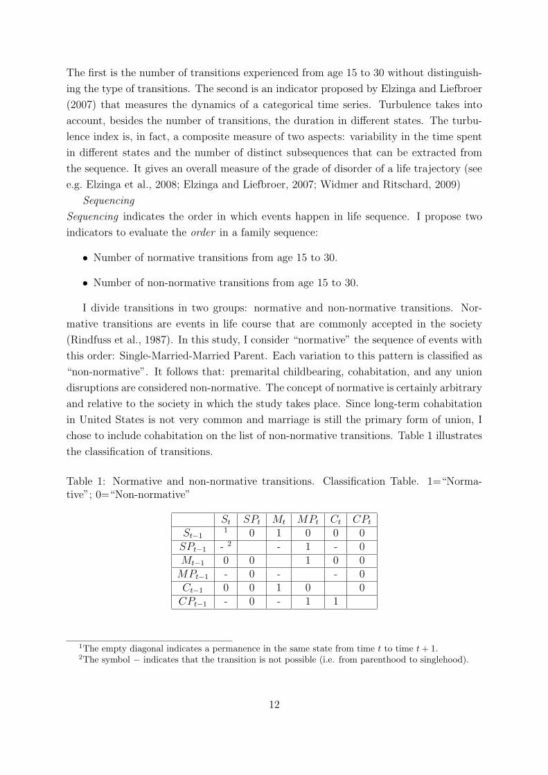
I divide transitions in two groups: normative and non-normative transitions. Nor-

mative transitions are events in life course that are commonly accepted in the society

(Rindfuss et al., 1987). In this study, I consider “normative” the sequence of events with

this order: Single-Married-Married Parent. Each variation to this pattern is classified as

“non-normative”. It follows that: premarital childbearing, cohabitation, and any union

disruptions are considered non-normative. The concept of normative is certainly arbitrary

and relative to the society in which the study takes place. Since long-term cohabitation

in United States is not very common and marriage is still the primary form of union, I

chose to include cohabitation on the list of non-normative transitions. Table 1 illustrates

the classification of transitions.

Table 1: Normative and non-normative transitions. Classification Table. 1=“Norma-tive”; 0=“Non-normative”

St SPt Mt MPt Ct CPt

St−11 0 1 0 0 0

SPt−1 - 2 - 1 - 0Mt−1 0 0 1 0 0MPt−1 - 0 - - 0Ct−1 0 0 1 0 0CPt−1 - 0 - 1 1

1The empty diagonal indicates a permanence in the same state from time t to time t + 1.2The symbol − indicates that the transition is not possible (i.e. from parenthood to singlehood).

12

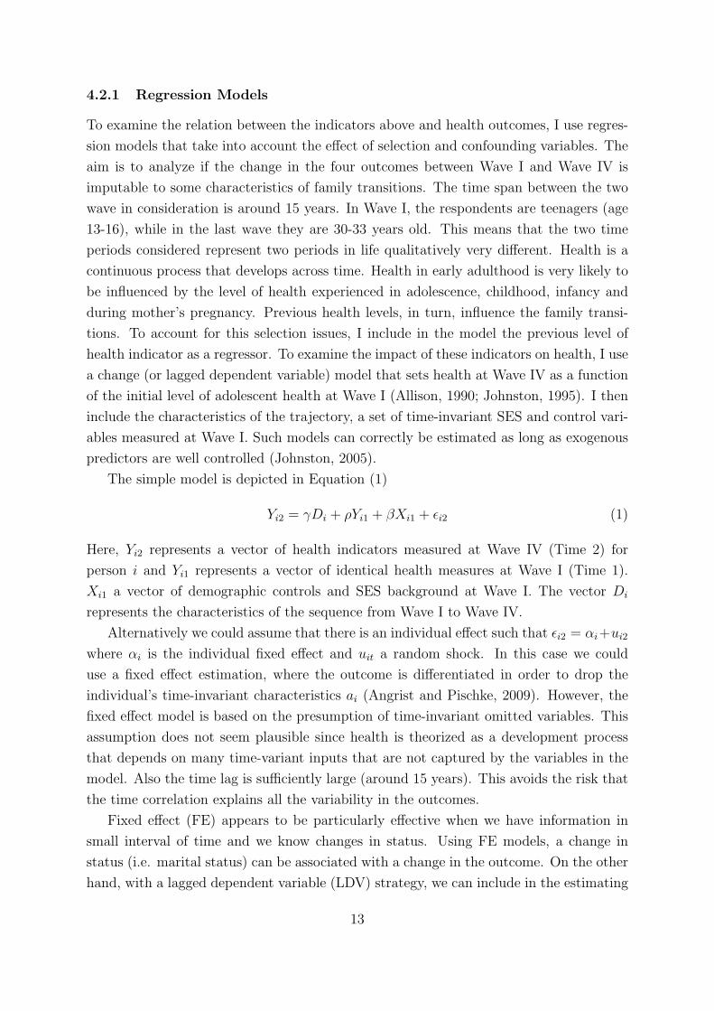
4.2.1 Regression Models

To examine the relation between the indicators above and health outcomes, I use regres-

sion models that take into account the effect of selection and confounding variables. The

aim is to analyze if the change in the four outcomes between Wave I and Wave IV is

imputable to some characteristics of family transitions. The time span between the two

wave in consideration is around 15 years. In Wave I, the respondents are teenagers (age

13-16), while in the last wave they are 30-33 years old. This means that the two time

periods considered represent two periods in life qualitatively very different. Health is a

continuous process that develops across time. Health in early adulthood is very likely to

be influenced by the level of health experienced in adolescence, childhood, infancy and

during mother’s pregnancy. Previous health levels, in turn, influence the family transi-

tions. To account for this selection issues, I include in the model the previous level of

health indicator as a regressor. To examine the impact of these indicators on health, I use

a change (or lagged dependent variable) model that sets health at Wave IV as a function

of the initial level of adolescent health at Wave I (Allison, 1990; Johnston, 1995). I then

include the characteristics of the trajectory, a set of time-invariant SES and control vari-

ables measured at Wave I. Such models can correctly be estimated as long as exogenous

predictors are well controlled (Johnston, 2005).

The simple model is depicted in Equation (1)

Yi2 = γDi + ρYi1 + βXi1 + εi2 (1)

Here, Yi2 represents a vector of health indicators measured at Wave IV (Time 2) for

person i and Yi1 represents a vector of identical health measures at Wave I (Time 1).

Xi1 a vector of demographic controls and SES background at Wave I. The vector Di

represents the characteristics of the sequence from Wave I to Wave IV.

Alternatively we could assume that there is an individual effect such that εi2 = αi+ui2

where αi is the individual fixed effect and uit a random shock. In this case we could

use a fixed effect estimation, where the outcome is differentiated in order to drop the

individual’s time-invariant characteristics ai (Angrist and Pischke, 2009). However, the

fixed effect model is based on the presumption of time-invariant omitted variables. This

assumption does not seem plausible since health is theorized as a development process

that depends on many time-variant inputs that are not captured by the variables in the

model. Also the time lag is sufficiently large (around 15 years). This avoids the risk that

the time correlation explains all the variability in the outcomes.

Fixed effect (FE) appears to be particularly effective when we have information in

small interval of time and we know changes in status. Using FE models, a change in

status (i.e. marital status) can be associated with a change in the outcome. On the other

hand, with a lagged dependent variable (LDV) strategy, we can include in the estimating

13

equation time-invariant variables. While FE models control for time-invariant omitted

variables, LDV model does not. In particular, this can lead to bias in the estimates if we

attempt in identifying a causal effect of a treatment variable. However, in this case, the

proposed estimation strategy seems to be a good compromise to give a portrait of the

statistical association between trajectories and health outcomes.

4.2.2 Extracting typologies of life trajectories

The indicators proposed in the previous paragraph are useful to describe some charac-

teristics of the life trajectory. However, they do not give any indication on the “type”

of sequence. To describe completely family trajectories we need to study simultaneously

timing, quantum, and sequencing in life course sequences (Billari, 2005). The complexity

of life course suggests to adopt an holistic approach, where all the different components of

the life course are taken into account. Abbott (1995) was the first to introduce sequence

analysis in the social sciences using Optimal Matching algorithm (OM) as a method to

compare different life sequences. This method has been used for the alignment of biose-

quences. The basic idea behind optimal matching is to measure the dissimilarity of two

sequences by considering how much effort is required to transform one sequence into the

other one. Transforming sequences entails three basic operations in this very elementary

method:

• insertion

• deletion

• substitution

A specific cost can be assigned to each operation, and the total cost of applying a series

of elementary operations can be computed as the sum of the costs of single operations.

Thus, the distance between two sequences can be defined as the minimum cost of trans-

forming one sequence into the other one. Hence, the resulting output is a symmetric

matrix of pairwise distances that can be used for further statistical analysis, mainly

multivariate analysis. Optimal Matching is a family of dissimilarity measures between

sequences derived from the distance originally proposed in the field of information theory

and computer science by Vladimir Levenshtein (Levenshtein, 1965), with the difference

that in OM the three operations have different costs, (Lesnard, 2006). The choice of the

operations’ costs determines the matching procedure and influences the results obtained.

This is a major concern about the use of this technique in social sciences (Wu, 2000). A

common solution for assessing the substitution costs is to use the inverse of the transition

probability, in order to assign higher costs to the less common transitions (Piccarreta and

Billari, 2007). I adopt this strategy in the empirical analysis.

14

Sequence analysis have been adopted in demography to study complex phenomenon in

order to simultaneously study multiple demographic transitions (see e.g. Billari, 2001).

Once obtained the dissimilarity matrix, we can apply standard reduction techniques

to classify trajectories into homogeneous groups. The resulting groups are then used

to describe “typical” patterns of transitions. Following the approach of McVicar and

Anyadike-Danes (2002), I conduct a cluster analysis using Ward algorithm to identify

six clusters of life sequences. Clusters can be described by choosing a representative se-

quence. Aassve et al. (2007) suggest to identify groups by using the medoid sequence, that

is the sequence with the minimum distance from all of the other sequences in that cluster.

This group characterization of life sequences can be used as an input for further

analysis, in particular regression analysis in order to explore the consequences of different

life trajectories. For instance, Mouw (2005) uses the output of a clustering procedure

as an input for a regression analysis under the heading “Does the sequence matter?”

Regression analyses show important differences in the risk of experiencing outcomes such

as poverty at age 35. Sequences are also found to influence subsequent happiness and

depression status.

In this study, I analyze the consequences of family trajectories on health outcomes.

I detect typical trajectories using cluster analysis on family sequences from age 15 to

age 30. I only consider sequences from age 15-30 in order to have sequences of the same

length for all the individuals. The resulting groups are then used as a categorical variable

in a regression analysis. Using different “typologies” of trajectory allows to analyze the

change in health status among different groups of individuals. This clustering procedure,

for instance, allows to isolate the groups of single mothers who experience the birth of

the first child outside a union, and do not experience stable union after childbearing.

It is important, from a policy point of view to understand if any particular trajectory

is associated with a decrease in health status. However, health status is measured at

different ages for different individuals. This creates an asynchrony between the outcome

and the time used to describe the covariate. The ideal situation, would be to have

individuals interviewed at the same age. To control for age effects I introduce age and

age-squared in the estimation.

5 Analysis of trajectories

It is important to examine events in the initial years of early adulthood because the

large-scale changes in cohabitation, marriage, and non marital fertility have particularly

affected women in age 20-30. In terms of family transitions,those years are very “dense”

(Rindfuss, 1991), with more demographic events occurring than during any other part

15

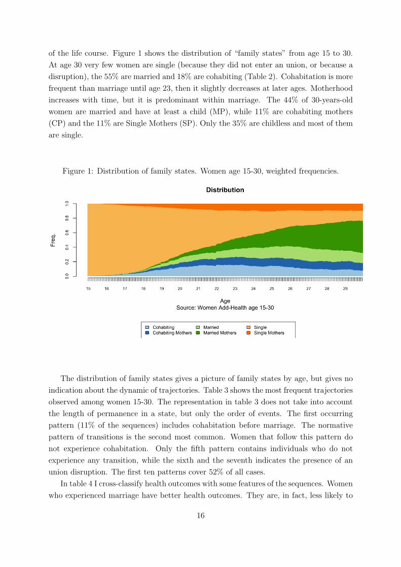
of the life course. Figure 1 shows the distribution of “family states” from age 15 to 30.

At age 30 very few women are single (because they did not enter an union, or because a

disruption), the 55% are married and 18% are cohabiting (Table 2). Cohabitation is more

frequent than marriage until age 23, then it slightly decreases at later ages. Motherhood

increases with time, but it is predominant within marriage. The 44% of 30-years-old

women are married and have at least a child (MP), while 11% are cohabiting mothers

(CP) and the 11% are Single Mothers (SP). Only the 35% are childless and most of them

are single.

Figure 1: Distribution of family states. Women age 15-30, weighted frequencies.

The distribution of family states gives a picture of family states by age, but gives no

indication about the dynamic of trajectories. Table 3 shows the most frequent trajectories

observed among women 15-30. The representation in table 3 does not take into account

the length of permanence in a state, but only the order of events. The first occurring

pattern (11% of the sequences) includes cohabitation before marriage. The normative

pattern of transitions is the second most common. Women that follow this pattern do

not experience cohabitation. Only the fifth pattern contains individuals who do not

experience any transition, while the sixth and the seventh indicates the presence of an

union disruption. The first ten patterns cover 52% of all cases.

In table 4 I cross-classify health outcomes with some features of the sequences. Women

who experienced marriage have better health outcomes. They are, in fact, less likely to

16

Table 2: Weighted age percentage of women for marital status, cohabitation and moth-erhood from age 16 to age 30.

AgeProp. Prop. Prop.

married cohabiting with children16 0.00 0.01 0.0117 0.00 0.03 0.0318 0.02 0.07 0.0619 0.06 0.14 0.1120 0.11 0.19 0.1721 0.14 0.23 0.2322 0.19 0.25 0.2923 0.25 0.27 0.3524 0.32 0.25 0.3825 0.37 0.26 0.4426 0.44 0.24 0.4927 0.50 0.21 0.5228 0.52 0.21 0.5729 0.55 0.21 0.6230 0.55 0.18 0.62

Table 3: First 10 sequence pattern of transitions in Women 15-30. Weighted frequencies.

Freq1 S-C-M-MP 11.462 S-M-MP 10.463 S-C-M 5.934 S-C-CP-MP 4.415 S 4.376 S-C-S 3.467 S-C-S-C-M-MP 3.378 S-M 3.159 S-C 3.0710 S-SP-CP-MP 2.77

Pattern representation indicates the sequence of events with durations ≥ 1

report poor health, to suffer depression and adopt more healthy behaviors. On the

contrary, women that have at least a cohabitation experience are more likely to have

poor health. Furthermore, the proportion of smokers and heavy drinkers is greater among

cohabiting and unmarried people. We do not observe great differences between mothers

and non-mothers on self-reported health and depression. We observe, instead, differences

17

in behaviors. In fact, mothers are less likely to be smokers or to drink than women who

never had a child.

Table 4: Proportion of women in poor health, with depression symptoms, smoking andheavy drinking in the last 30 days. Frequencies by union status and motherhood.

Prop. with Prop. with Prop. Prop.poor health depression symptoms smoking drinking

Never Married 0.11 0.20 0.39 0.45Ever Married 0.09 0.15 0.27 0.32Never Cohabitation 0.07 0.17 0.16 0.20Ever Cohabitation 0.10 0.17 0.36 0.42Non-mothers 0.10 0.17 0.29 0.45Mothers 0.10 0.17 0.32 0.32Total 0.11 0.18 0.27 0.35

Although these descriptive tables show a relation between health and family status,

the true impact can be masked by selection issues and by the effect of confounding vari-

ables. In table 5 I report the mean value of indicators of timing, quantum, and sequences

for women conditional to their health status. Individuals with poor health status and

depression symptoms have their first family transitions earlier than others. They usually

experience more transitions, in particular the “non-normative” ones. Analogously, smok-

ing and drinking behavior is associated with early exit from singlehood, younger age at

first union and first child and greater number of non-normative transitions.

18

Table 5: Indicators of timing, quantum and sequencing and health status.

Poor Health Depression Smoking Drinking Totalno yes no yes no yes no yes

Timing indicatorsAge at first transition 22.12 21.17 22.12 21.17 22.47 20.83 22.06 21.83 21.97Age at first union 22.24 21.02 22.23 21.02 22.55 20.96 21.91 22.03 21.96Age at first child 23.44 21.99 23.51 21.99 23.80 22.01 23.54 23.18 23.43

Quantum indicatorsNumber of transition 3.09 3.40 3.11 3.41 2.9 3.69 3.08 3.36 3.18Turbulence 6.43 6.48 6.45 6.48 6.27 6.89 6.42 6.68 6.52

Sequencing indicatorsNumber of normativetransition

1.08 0.97 1.10 0.97 1.12 0.93 1.19 0.96 1.10

Number of non-normative transition

2.02 2.43 2.01 2.44 1.80 2.80 1.897 2.40 2.08

19

5.1 Multivariate results

Early transitions have a negative effect on self-reported health and smoking behavior.

Table 6 (and tables 12,13 in the appendix) reports the results of the regression analysis.

These results indicate that, controlling for previous health and compositional character-

istics, transitions under age 18 are associated with poor self-reported health and increase

in smoking. If we consider only union transitions or the age at first child, also transi-

tions before age 20 are significantly different from transitions that happen later in life.

Moreover, depression symptoms are associated with early childbearing. The dynamic of

family trajectories has a similar effect. The number of transitions is associated with neg-

ative effect on self-reported health and smoking behavior. The more transition a woman

experience between wave I and wave IV, the more she is likely to smoke and report poor

health (see table 7). Other indicators of sequence dynamics, instead, do not show notable

effect on health outcomes (see table 14 in the appendix).

It is interesting to notice, however, what happens if we decompose the number of tran-

sitions into normative and non-normative (the distinction between normative transitions

and non-normative is defined in table 1). Results in table 8 show that the two types of

sequences have an opposite effect. While non-normative transitions have a negative effect

on health outcomes, normative transitions are associated with less unhealthy behavior.

Non-normative transitions are associated with a decrease in self-reported health and an

increase in depression symptoms. Concerning smoking and drinking behaviors, we ob-

serve a protection effect given by normative transitions. Traditional family formation is

therefore associated with reduction of risky behaviors. Controlling for other variables,

non-normative transitions are associated with increase in the number of cigarette smoked

and drinking occasions. Possible explanations are that non-normative transitions consti-

tute major sources of stress. People who follow a normative path, instead, receive bigger

support from friends and family.

The estimate results in tables 6,7,8 show similar levels of correlation between health

outcomes in Wave I and Wave IV. The inclusion of lagged dependent variable allows to

take into account selection issues. I also included in the models’ background variables

indicating race composition, socio-economic status and the family composition at the be-

ginning of the transition. Although previous health outcomes control for health selection,

I assume that background characteristics can affect the level of health at Wave IV net

of previous health outcomes. Estimates show that women with college educated parents

have lower health outcomes and minor propensity to smoke. The propensity to engage

in risky behavior changes with race. Black and Hispanic girls tend to smoke and drink

less than their white counterpart. Moreover, African American women have a general

tendency to report minor levels of health. Overall, these results show that women that

20

move away from a traditional pattern have bigger risk to report poor health and above

all to engage in risky behaviors. Therefore, these results show that timing, quantum and

sequencing are important factors in the study of family formation.

6 Typologies of family trajectories

The analyses presented in the previous section show that women who move away from

a “normative” model (especially in terms of age at first transition and order of events)

are the ones who experienced greater decline on health status. Poor health outcomes are

associated with early transitions, high numbers of changes in family status, and “non-

normative” order of events. Traditional transitions seem to have instead a protective

effect, especially on behavior.

Any how, previous analysis do not permit to identify what type of family patterns are

associated with changes in health status. From a policy point of view, we are interested in

detecting what subgroups of population risk more to experience poor health, for example,

single motherhood (Furstenberg, 2005, 1998, 1976). Previous studies show lower levels of

health among single mothers, in particular mental health (Cairney et al., 2003), propen-

sity to smoke (Francesconi et al., 2010), and also higher level of mortality, (Mirowsky,

2005). Therefore, it is relevant to study the consequences of different patterns in family

formation.

The number of possible combinations of sequences in family formation is almost un-

limited. It follows that a convenient empirical strategy aims to reduce all the possible

trajectories to a more manageable number. I used a cluster analysis to specify six groups

of trajectories as representative of the entire set of sequences. The details of the analysis

are presented in the Appendix. Below, I present a description of the sequences in each

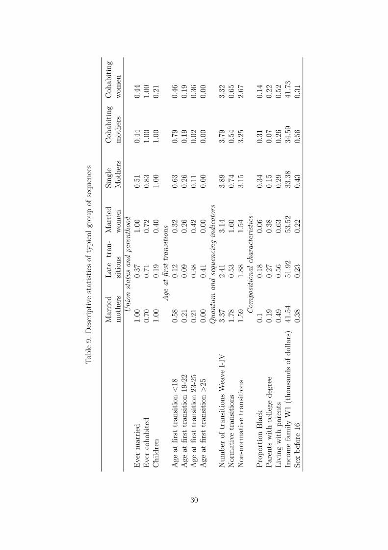
group, additional details can be found in table 9 and figures 2 and 3. Clusters can also be

described using their medoid sequences (Aassve et al., 2007). A medoid is the observation

with the minimum distance from other individuals in a cluster. The advantage of using

medoid sequences is to define the cluster using a real sequence that best represents the

groups.

1. Married mothers (S,73)(C,11)(M,12)(MP,84); n=693. This is the largest group

in the sample (29%). It is composed by women that follow a more traditional

pattern, i.e. Single-Married-Married Mothers. Almost all of them experience both

marriage and motherhood. Cohabitation is not rare, but generally short. Women

in this class start family transition earlier than women in other groups (with the

exception of single and cohabiting mothers). Although the number of transitions

is comparable with the other groups, the number of “non-normative” transitions is

21

Table 6: Regression estimates. Effects of timing indicators on health outcomes: age atfirst transition

(1) (2) (3) (4)Poor

Health Depression Smoking Drinking

Age at first transition > 25 (ref.)Age at first transition < 18 0.270∗∗ 0.295 3.278∗∗∗ 0.0697

(0.102) (0.496) (0.871) (0.102)

Age at first transition 18-20 0.128 0.0691 1.771 0.0525(0.107) (0.524) (0.916) (0.107)

Age at first transition 20-25 −0.0214 −0.0373 0.761 0.100(0.104) (0.503) (0.841) (0.104)

Age at wave I 0.683 −4.167 −12.23 0.866(0.904) (5.361) (11.98) (0.666)

Age squared at wave I −0.0199 0.112 0.310 −0.0268(0.0251) (0.147) (0.329) (0.0180)

Living with bio-parents at wave I −0.0383 −0.185 −1.082 −0.00895(0.0533) (0.250) (0.640) (0.0738)

College educated parents −0.230∗∗∗ −0.717∗∗ −3.151∗∗∗ 0.0685(0.0636) (0.273) (0.771) (0.0949)

Hispanic 0.184∗ −0.112 −3.544∗∗∗ −0.150(0.0905) (0.437) (0.755) (0.0943)

Black 0.176∗∗ 0.567 −1.002 −0.278∗∗∗

(0.0618) (0.342) (0.770) (0.0795)

Asian 0.208 0.0783 −1.643 −0.0998(0.120) (0.389) (1.242) (0.155)

Self-reported health at wave I 0.270∗∗∗

(0.0289)

Depression WI 0.277∗∗∗

(0.0259)

Smoking WI 0.509∗∗∗

(0.0318)

Drinking WI 0.177∗∗∗

(0.0275)

Constant −4.230 42.61 123.8 −6.337(8.132) (48.88) (109.3) (6.181)

Observations 2255 2237 2237 2248Adjusted R2 0.141 0.108 0.310 0.060Standard errors in parentheses∗ p < 0.05, ∗∗ p < 0.01, ∗∗∗ p < 0.001

22

Table 7: Regression estimates. Effects of quantum indicators on health outcomes: numberof transitions

(1) (2) (3) (4)Poor


Number of transitions 0.0457∗∗ 0.122 0.674∗∗∗ 0.0151(0.0149) (0.0748) (0.183) (0.0192)

Age at wave I 0.325 −12.63∗ −30.34∗ 0.529(1.475) (5.981) (14.84) (1.113)

Age squared at wave I −0.0102 0.343∗ 0.805∗ −0.0175(0.0406) (0.164) (0.405) (0.0299)



Hispanic 0.182∗ −0.0408 −3.426∗∗∗ −0.144(0.0917) (0.435) (0.747) (0.0953)

Black 0.175∗∗ 0.579 −0.963 −0.274∗∗∗

(0.0619) (0.341) (0.783) (0.0813)

Asian 0.198 0.0574 −1.785 −0.102(0.117) (0.377) (1.252) (0.156)


(0.0292)


(0.0255)


(0.0321)


(0.0273)

Constant −0.915 119.5∗ 289.0∗ −3.257(13.40) (54.53) (135.9) (10.36)


23

Table 8: Regression estimates. Effects of sequencing indicators on health outcomes:number of normative and non-normative transitions

(1) (2) (3) (4)Poor


Number of normative transitions −0.0180 −0.133 −1.122∗∗ −0.216∗∗∗

(0.0315) (0.144) (0.354) (0.0430)

Number non-normative transitions 0.0556∗∗∗ 0.160∗ 0.961∗∗∗ 0.0513∗

(0.0153) (0.0769) (0.205) (0.0203)

Age at wave I 0.432 −12.21∗ −26.79∗ 0.988(1.460) (5.933) (13.40) (1.105)

Age squared at wave I −0.0131 0.332∗ 0.710 −0.0298(0.0401) (0.162) (0.364) (0.0297)

Living with bio-parents at wave I −0.0459 −0.115 −0.796 0.0575(0.0540) (0.253) (0.657) (0.0740)


Hispanic 0.163 −0.121 −4.121∗∗∗ −0.216∗

(0.0912) (0.435) (0.752) (0.0994)

Black 0.136∗ 0.425 −2.251∗∗ −0.425∗∗∗

(0.0640) (0.346) (0.815) (0.0862)

Asian 0.195 0.0529 −1.984 −0.124(0.117) (0.384) (1.207) (0.144)


(0.0290)


(0.0256)


(0.0327)


(0.0271)

Constant −1.861 115.8∗ 257.3∗ −7.337(13.27) (54.10) (123.1) (10.26)


24

limited.

2. Late transitions (S,168)(C,12); n=648. This group represents women that start

family transition very late or the ones who have not experienced any transition

by age 30. They stay single for the majority of the sequence and they eventually

experience a transition to cohabitation. Very few of them are married or have a

child by age 30.

3. Married women without children (S,97)(C,12)(M,71); n=315. This group

differs from group 1 essentially for two reasons. Women in this group begin the

family transition later and they remain longer married without a child. The average

time in which they stay married without children (M) is 2 years and half, compared

to 1 year in group 1. The result is that the majority of women in this group

postpones childbearing after age 30. The majority of transitions is traditional

and cohabitation is generally short. Above all, this group is characterized by a

postponement of traditional pattern.

4. Single Mothers (S,71)(SP,90)(CP,19); n=302. This group identifies women who

became mothers without being in an partnership. The group is characterized by

very early transition to motherhood. Although there are some experiences of cohab-

itation, most of the time is spent outside a union. Women in this group experience

in average more transitions than women in other groups. The majority of transi-

tions are non-traditional. Single mothers are more likely to experience more than

one cohabitation union.

5. Cohabiting mothers (S,59)(C,15)(CP,106); n=237. Women in this group differ

from single mothers mainly for the fact that childbearing occurs during a cohabita-

tion. This group is characterized by early transitions both to union and to moth-

erhood. Similarly to single mothers, they experience a large number of transitions,

most of them “non-normative” transitions.

6. Cohabitating women (S,92)(C,84)(M,4); n=163. The last group is characterized

by cohabitation. It accounts for roughly 7% of women in the sample. Trajectories

in this class are similar to group 2 (late transitions), with the difference that women

in this group anticipate union to enter a cohabitation. The number of transitions

is relatively low. Childbearing is postponed to later age.

Groups differ for compositional characteristics, in particular race composition and

socioeconomic status (see table 9). Groups 4 and 5 have a higher proportion of African

25

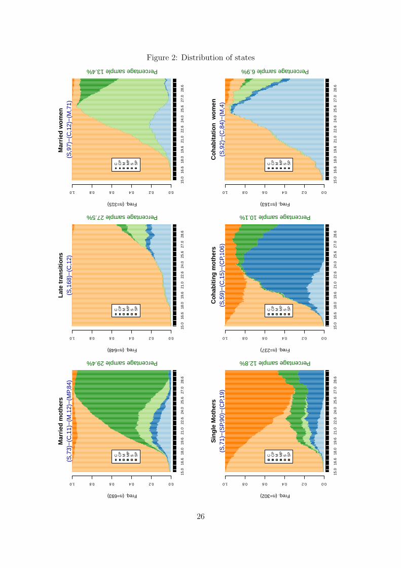
Figure 2: Distribution of statesM

arrie

d m

othe

rs

Freq. (n=693)

15.0

16.6

18.0

19.6

21.0

22.6

24.0

25.6

27.0

28.6

0.00.20.40.60.81.0

C CP

M MP

S SP

Percentage sample 29.4%

(S,7

3)−

(C,1

1)−

(M,1

2)−

(MP,

84)

Late

tran

sitio

ns

Freq. (n=648)

15.0

16.6

18.0

19.6

21.0

22.6

24.0

25.6

27.0

28.6

0.00.20.40.60.81.0

C CP

M MP

S SP


(S,1

68)−

(C,1

2)M

arrie

d w

omen

Freq. (n=315)

15.0

16.6

18.0

19.6

21.0

22.6

24.0

25.6

27.0

28.6

0.00.20.40.60.81.0

C CP

M MP

S SP


(S,9

7)−

(C,1

2)−

(M,7

1)

Sin

gle

Mot

hers

Freq. (n=302)

15.0

16.6

18.0

19.6

21.0

22.6

24.0

25.6

27.0

28.6

0.00.20.40.60.81.0

C CP

M MP

S SP


(S,7

1)−

(SP,

90)−

(CP,

19)

Coh

abiti

ng m

othe

rsFreq. (n=237)

15.0

16.6

18.0

19.6

21.0

22.6

24.0

25.6

27.0

28.6

0.00.20.40.60.81.0

C CP

M MP

S SP


(S,5

9)−

(C,1

5)−

(CP,

106)

Coh

abita

tion

wom

en

Freq. (n=163)

15.0

16.6

18.0

19.6

21.0

22.6

24.0

25.6

27.0

28.6

0.00.20.40.60.81.0

C CP

M MP

S SP


(S,9

2)−

(C,8

4)−

(M,4

)

26

American women. These two groups seem to be the more disadvantaged in terms of

family resources. Their families’ income is noticeably inferior and a great proportion of

them was not living with two biological parents at Wave I. On the contrary, women in

the groups 2 and 3 seem to be more advantaged in terms of family income, education and

family composition.

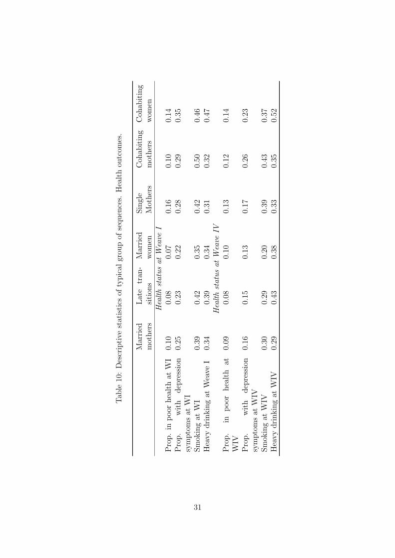
Single mothers, cohabiting mothers and cohabiting women (groups 3,4 and 6) report

inferior level of health at Wave IV (table 6). The same groups also have higher probability

to incur depression symptoms. This is partially explained by selection, since the same

groups also have lower levels of health during wave I. Single and cohabiting mothers

have a greater propensity to smoke at Wave IV. Drinking behavior, instead, is more

frequent among cohabiting women and women who experience late transitions. Although

we observe a general reduction in smoking from adolescent to adulthood, women who

postpone family transitions (group 2) are the ones who have the biggest decrease.

To investigate the relation between health and family trajectories, I applied the same

estimation strategy used in the previous section. Since family trajectories are subject to

selection issues and confounding variables, I control for previous health outcomes (Wave

I) and compositional characteristics in the regression models. The choice of the family

pattern is very likely to be influenced by variables that are omitted in the regression

model. Also the effect of reverse causation may not be negligible. On the other hand, the

dependent variable is only a representation of a variety of trajectories and it cannot be

thought as a treatment that is randomly assigned to the population. For this reason, the

estimation results presented in table 11 only indicate a statistical association and they

not have a causal significance. Nevertheless, results show some interesting aspects of the

relation between health and family formation.

First, both women who have a child in early age and the ones who cohabit without

children have lower self-reported health. On the other hand, women with a traditional

pattern do not differ significantly to women who postpone family transitions. Second,

cohabiting mothers are more likely to experience depression symptoms compared to other

groups. Although single mothers are similar in many aspects, they do not differ from the

reference group. A possible explanation is that depression is associated with the cohab-

iting experience, or in other terms with union instability. Last, smoking and drinking

behaviors appear to be strongly influenced by family patterns. Trajectories with marriage

seem to have a protective effect on the risky behaviors of women. Controlling for other

variables, women of group 1 and 2 have lower probability to engage in heavy drinking

behavior, while women of group 2 experience a sensible reduction on the average number

of cigarette smoked. This is consistent with other studies that show how marriage has

27

a strong incentive on reducing risky behaviors (Duncan et al., 2006). However, it would

be interesting to understand if this protective effect remains constant in time or if it has

only a temporary effect. Overall, parents education has a positive effect on health - both

physical and mental - and a reduction on cigarette smoking. Race has a mixed effect.

Black women report less perceived health levels, but at the same time are less likely to

engage in drinking behavior.

7 Discussion

Health is the result of a continuous process that develops over an individual’s lifetime.

Health trajectories are the consequence of a multitude of factors coming from genetic, bi-

ological, behavioral, social and economic contexts. Previous studies indicate that health

is certainly connected with family events occurring during life course. Following the

approach of Giele and Elder (1998), I distinguish between transitions (changes in family

status) and trajectories (the whole sequence of transitions) in order to study jointly union

formations and childbearing. Although the study of the dynamic inter-relationship be-

tween health and the life course has recently been an emerging topic, there is no general

agreement on how trajectories should be conceptualized and analyzed. In this paper, I

use sequence analysis to describe life course trajectories. Describing family biographies

as sequences of family states allows to analyze different dimensions of life course. In

particular, I am interested in examining if there is a direct effect of timing, quantum

and sequencing on health outcomes for young women. It emerges that, controlling for

selection and background characteristics, changes in these dimensions affect health sta-

tus. Early transitions have negative repercussions on self-reported health and smoking

behavior (hypothesis 1 ). Although the experience of a large number of transitions is asso-

ciated with negative effects (hypothesis 2 ), some particular transitions have a protective

effect. Normative transitions (i.e. traditional unions, childbearing after marriage) have

protective effects on behaviors (hypothesis 3 ). Women with numerous normative transi-

tions, in fact, smoke less cigarettes and have less occasions of heavy drinking. Above all,

the indicators proposed indicate that sequence characteristics matters. In particular, it

seems that moving away from normative family patterns (in terms of age-roles and order

of events) is associated with a decrease in wellbeing.

In the second part of the paper, I examine the consequences of different typology of

trajectories. I individuate six classes representing typical patterns of family formation.

Differences in terms of wellbeing and propensity to risky behaviors are substantial. Once

controlled for selection and background characteristics, these differences are attenuated

but still significant. Empirical results show that women with short experiences of cohab-

itation and women with a traditional pattern do not differ significantly to women who

28

postpone family transitions. On the other hand, early childbearing and long cohabitation

are associated with poor health status. Moreover, married women are less likely to smoke

and to drink. These analyses partially confirm previous studies, in particular regarding

the “protection effect” of marriage. Although selection and social background play most

of the role, we still observe negative outcomes for women who experience early childbear-

ing. We do not find much differences, instead, between single mothers and young mothers

that have a child during a cohabitation.

Results show that early childbearing is associated with worse health outcomes. It is

possible that women who anticipate motherhood have less resources (in terms of human

and social capital) to tackle the stress of raising a child (especially if without a stable

partner). Another complementary explanation is that early mothers are disadvantaged in

the marriage market and they have difficulties to match with good men. Our results also

show that married women are less likely to smoke and drink, confirming a “protection

effect” of marriage. Cohabitation seems to have no negative effect if short and followed by

a marriage. On the other hand, it is associated to poor outcomes (especially propensity

to smoking and drinking) when it is persistent and accompanied by motherhood. It is

possible, in fact, that short cohabitation, when followed by marriage, are becoming more

and more accepted in the society. The aim of this paper is mainly descriptive. The

mechanism of these relations, in fact, is beyond the scope of this work. Nevertheless,

these results, give evidences that family trajectories matter.

It would be interesting in the future, to investigate if these differences persist during

the life course to see if the more disadvantaged groups are able to catch up with the others.

Another open issue is the interaction between family transitions and social class. It may

be, in fact, that family trajectories have different effects according to the socio-economic

status of the family of origin. For example, the risk associated with non-normative

transitions may not affect women coming from higher social class. Last, this study only

deals with young women and ignores men. Comparing the trajectories of partners might

help to understand the effect of previous family transitions in the marriage market. Any

how, this study represents one of the first tentative to study the association between

health and family formation using a life course perspective.

29

Tab

le9:

Des

crip

tive

stat

isti

csof

typic

algr

oup

ofse

quen

ces

Mar

ried

mot

her

sL

ate

tran

-si

tion

sM

arri

edw

omen

Sin

gle

Mot

her

sC

ohab

itin

gm

other

sC

ohab

itin

gw

omen

Un

ion

stat

us

and

pare

nth

ood

Eve

rm

arri

ed1.

000.

371.

000.

510.

440.

44E

ver

cohab

ited

0.70

0.71

0.72

0.83

1.00

1.00

Childre

n1.

000.

190.

401.

001.

000.

21A

geat

firs

ttr

ansi

tion

sA

geat

firs

ttr

ansi

tion

<18

0.58

0.12

0.32

0.63

0.79

0.46

Age

atfirs

ttr

ansi

tion

19-2

20.

210.

090.

260.

260.

190.

19A

geat

firs

ttr

ansi

tion

23-2

50.

210.

380.

420.

110.

020.

36A

geat

firs

ttr

ansi

tion

>25

0.00

0.41

0.00

0.00

0.00

0.00

Qu

antu

man

dse

quen

cin

gin

dica

tors

Num

ber

oftr

ansi

tion

sW

eave

I-IV

3.37

2.41

3.14

3.89

3.79

3.32

Nor

mat

ive

tran

siti

ons

1.78

0.53

1.60

0.74

0.54

0.65

Non

-nor

mat

ive

tran

siti

ons

1.59

1.88

1.54

3.15

3.25

2.67

Com

posi

tion

alch

arac

teri

stic

sP

rop

orti

onB

lack

0.1

0.18

0.06

0.34

0.31

0.14

Par

ents

wit

hco

lleg

edeg

ree

0.19

0.27

0.38

0.15

0.07

0.22

Liv

ing

wit

hpar

ents

0.49

0.56

0.63

0.29

0.26

0.52

Inco

me

fam

ily

W1

(thou

sands

ofdol

lars

)41

.54

51.9

253

.52

33.3

834

.59

41.7

3Sex

bef

ore

160.

380.

230.

220.

430.

560.

31

30

Tab

le10

:D

escr

ipti

vest

atis

tics

ofty

pic

algr

oup

ofse

quen

ces.

Hea

lth

outc

omes

.

Mar

ried

mot

her

sL

ate

tran

-si

tion

sM

arri

edw

omen

Sin

gle

Mot

her

sC

ohab

itin

gm

other

sC

ohab

itin

gw

omen

Hea

lth

stat

us

atW

eave

IP

rop.

inp

oor

hea

lth

atW

I0.

100.

080.

070.

160.

100.

14P

rop.

wit

hdep

ress

ion

sym

pto

ms

atW

I0.

250.

230.

220.

280.

290.

35

Sm

okin

gat

WI

0.39

0.42

0.35

0.42

0.50

0.46

Hea

vy

dri

nkin

gat

Wea

veI

0.34

0.39

0.34

0.31

0.32

0.47

Hea

lth

stat

us

atW

eave

IVP

rop.

inp

oor

hea

lth

atW

IV0.

090.

080.

100.

130.

120.

14

Pro

p.

wit

hdep

ress

ion

sym

pto

ms

atW

IV0.

160.

150.

130.

170.

260.

23

Sm

okin

gat

WIV

0.30

0.29

0.20

0.39

0.43

0.37

Hea

vy

dri

nkin

gat

WIV

0.29

0.43

0.38

0.33

0.35

0.52

31

Table 11: Regression estimates. Effects of family trajectories on health outcomes

(1) (2) (3) (4)Poor


Late transitions (ref. category)

Married mother 0.105 0.0705 −0.151 −0.311∗∗∗

(0.0694) (0.301) (0.768) (0.0880)

Married women 0.0824 0.168 −1.906∗ −0.225∗

(0.0784) (0.389) (0.913) (0.109)

Single mothers 0.245∗∗ −0.196 1.858 −0.162(0.0883) (0.442) (1.095) (0.113)

Cohabiting mothers 0.211∗ 0.995∗ 2.243 −0.154(0.0919) (0.498) (1.153) (0.123)

Cohabitation women 0.252∗ 0.887 0.327 0.330(0.118) (0.481) (1.824) (0.230)

Age at wave I 0.650 −4.052 −12.08 1.173(0.876) (5.366) (11.90) (0.645)

Age squared at wave I −0.0193 0.108 0.301 −0.0354∗

(0.0244) (0.147) (0.326) (0.0174)



Hispanic 0.152 −0.114 −4.162∗∗∗ −0.182(0.0916) (0.448) (0.775) (0.0980)

Black 0.126∗ 0.530 −1.945∗ −0.324∗∗∗

(0.0630) (0.350) (0.815) (0.0814)

Asian 0.198 −0.00107 −1.813 −0.134(0.121) (0.394) (1.185) (0.149)


(0.0294)


(0.0261)


(0.0318)


(0.0270)

Constant −3.769 41.85 126.0 −8.809(7.889) (48.93) (108.6) (5.973)


32

References

Aassve, A., F. C. Billari, and R. Piccarreta, 2007. Strings of Adulthood: A Sequence

Analysis of Young British Women’s Work-Family Trajectories. European Journal of

Population, 23(3-4):369–388.

Abbott, A., 1995. Sequence analysis: new methods for old ideas. Annual Review of

Sociology, 21(1):93–113.

Abbott, A. and A. Tsay, 2000. Sequence analysis and optimal matching methods in

sociology: Review and prospect. Sociological Methods & Research, 29(1):3.

Acs, G., 2007. Can We Promote Child Well-Being by Promoting Marriage? Journal of

Marriage and Family, 69(5):1326–1344.

Allison, P., 1990. Change Scores as Dependent Variables in Regression Analysis. Socio-

logical Methodology, 20:93–114.

Amato, P., 2007. Strengthening marriage is an appropriate social policy goal. Journal of

Policy Analysis and Management, 26(4):952–955.

Amato, P., N. Landale, and T. Havasevich-Brooks, 2008. Precursors of Young Women’s

Family Formation Pathways. Journal of Marriage and Family, 70:1271–1286.

Angrist, J. and J. Pischke, 2009. Mostly harmless econometrics: an empiricist’s compan-

ion. Princeton NJ:Princeton University Press.

Billari, F. C., 2001. The analysis of early life courses: complex descriptions of the tran-

sition to adulthood. Journal of Population Research, 18(2):119–142.

Billari, F. C., 2005. Life course analysis: two (complementary) cultures? Some reflections

with examples from the analysis of the transition to adulthood. Advances in Life Course

Research, 10:261–281.

Billari, F. C., J. Furnkranz, and A. Prskawetz, 2006. Timing, Sequencing, and Quantum

of Life Course Events: A Machine Learning Approach. European Journal of Population,

22(1):37–65.

Bumpass, L. and H.-H. Lu, 2000. Trends in Cohabitation and Implications for Children’s

Family Contexts in the United States. Population Studies, 54(1):29–41.

Bumpass, L., T. Martin, and J. Sweet, 1991. The impact of family background and early

marital factors on marital disruption. Journal of Family Issues, 12(1):22–42.

33

Cairney, J., M. Boyle, D. Offord, and Y. Racine, 2003. Stress, social support and depres-

sion in single and married mothers. Social Psychiatry and Psychiatric Epidemiology,

38:442 – 449.

Cherlin, A., 2004. The Deinstitutionalization of American Marriage. Journal of Marriage

and Family, 66(4):848–861.

Cherlin, A., 2005. American Marriage in the Early Twenty-First Century. The Future of

Children, 15(2):33–55.

Duncan, G., W. Bessie, and E. Paula, 2006. Cleaning Up Their Act: The Effects of

Marriage and Cohabitation on Licit and Illicit Drug Use. Demography, 43(4):691–710.

Dupre, M. E., A. N. Beck, and S. O. Meadows, 2009. Marital trajectories and mortality

among US adults. American Journal of Epidemiology, 170(5):546–55.

Edin, K. and J. Reed, 2005. Why Don’t They Just Get Married? Barriers to Marriage

among the Disadvantaged. The Future of Children, 15(2):117–137.

Elder, G., 1994. Time, Human Agency, and Social Change: Perspectives on the Life

Course. Social Psychology Quarterly, 57(1):4–15.

Elder, G. H., 1985. Life course dynamics: trajectories and transitions, 1968-1980. Ithaca,

NY: Cornell Univ Press.

Elzinga, C. and A. Liefbroer, 2007. De-standardization of family-life trajectories of young

adults: A cross-national comparison using sequence analysis. European Journal of

Population, 23(3):225–250.

Elzinga, C., S. Rahmann, and H. Wang, 2008. Algorithms for subsequence combinatorics.

Theoretical Computer Science, 409(3):394–404. doi:10.1016/j.tcs.2008.08.035.

Ermisch, J. and D. Pevalin, 2005. Early Motherhood and Later Partnerships. Journal of

Population Economics, 18(3):469–489.

Ferree, M., 1990. Beyond Separate Spheres: Feminism and Family Research. Journal of

Marriage and Family, 52(4):866–884.

Francesconi, M., S. P. Jenkins, and T. Siedler, 2010. The effect of lone motherhood on

the smoking behavior of young adults. Health Economics, in press.

Furstenberg, F. F., 1976. Unplanned parenthood: the social consequences of teenage

childbearing. New York: Free Press.

34

Furstenberg, F. F., 1998. When Will Teenage Childbearing Become a Problem? The Im-

plications of Western Experience for Developing Countries. Studies in Family Planning,

29(2):246–253.

Furstenberg, F. F., 2005. Non-normative life course transitions: reflections on the signif-

icance of demographic events on lives. Advances in Life Course Research, 10:155–172.

George, L. K., 2009. Conceptualizing Life course trajectories. In G. H. Elder and J. Z.

Giele, editors, The Craft of Life Course Research. New York, NY: Guilford Press.

Giele, J. Z. and G. H. Elder, 1998. Methods of life course research: qualitative and

quantitative approaches. Los Angeles, CA: SAGE Publications.

Gove, W., 1972. The Relationship between Sex Roles, Marital Status, and Mental Illness.

Social Forces, 51(1):34–44.

Halfon, N. and M. Hochstein, 2002. Life Course Health Development: An Integrated

Framework for Developing Health, Policy, and Research. The Milbank Quarterly,

80(3):433–479.

Harris, K. M., H. Lee, and F. Deleone, 2010. Marriage and Health in the Transition

to Adulthood: Evidence for African Americans in the Add Health Study. Journal of

Family Issues, forthcoming.

Hogan, D., 1978. The Variable Order of Events in the Life Course. American Sociological

Review, 43(4):573–586.

Horwitz, A. and H. White, 1998. The Relationship of Cohabitation and Mental Health:

A Study of a Young Adult Cohort. Journal of Marriage and Family, 60(2):505–514.

Johnston, D., 1995. Alternative Methods for the Quantitative Analysis of Panel Data

in Family Research: Pooled Time-Series Models. Journal of Marriage and Family,

57(4):1065–1077.

Johnston, D., 2005. Two-wave panel analysis: Comparing statistical methods for studying

the effects of transitions. Journal of Marriage and Family, 67(4):1061–1075.

Koball, H., E. Moiduddin, and J. Henderson, 2010. What Do We Know About the Link

Between Marriage and Health? Journal of Family Family, forthcoming.

Lamb, K., G. Lee, and A. DeMaris, 2003. Union Formation and Depression: Selection

and Relationship Effects. Journal of Marriage and Family, 65(4):953–962.

Lehrer, E., 1988. Determinants of marital instability: A Cox-regression model. Applied

Economics, 20(2):195 – 210.

35

Lesnard, L., 2006. Optimal matching and social sciences. Manuscript, Observatoire

Sociologique du Changement (Sciences Po and CNRS), Paris.(http://laurent. lesnard.

free. fr/).

Levenshtein, V. I., 1965. Binary codes capable of correcting deletions, insertions, and

reversals. Soviet Physics Dokl., 10:707–710.

Lichter, D., D. Graefe, and J. Brown, 2003. Is Marriage a Panacea? Union Formation

among Economically Disadvantaged Unwed Mothers. Social Problems, 50(1):60–86.

Liefbroer, A. and E. Dourleijn, 2006. Unmarried cohabitation and union stability: testing

the role of diffusion using data from 16 European countries. Demography, 43(2):203–

221.

Lillard, L., M. Brien, and L. Waite, 1995. Premarital Cohabitation and Subsequent

Marital Dissolution: A Matter of Self-Selection? Demography, 32(3):437–457.

Lillard, L. and L. Waite, 1993. A Joint Model of Marital Childbearing and Marital

Disruption. Demography, 30(4):653–681.

Macmillan, R., 2005. The structure of the life course: classic issues and current contro-

versies. Advances in Life Course Research, 9:3–24.

Martin, T. and L. Bumpass, 1989. Recent Trends in Marital Disruption. Demography,

26(1):37–51.

Mazzuco, S., 2009. Another look into the effect of premarital cohabitation on duration

of marriage: an approach based on matching. Journal of the Royal Statistical Society

Series A, 172(1):255–273.

McLanahan, S., 2007. Should government promote marriage? Journal of Policy Analysis

and Management, 26(4):951–964.

McVicar, D. and M. Anyadike-Danes, 2002. Predicting Successful and Unsuccessful Tran-

sitions from School to Work by Using Sequence Methods. Journal of the Royal Statis-

tical Society. Series A, 165(2):317–334.

Meadows, S., 2009. Family Structure and Fathers’ Well-Being: Trajectories of Mental

Health and Self-Rated Health. Journal of Health and Social Behavior, 50(2):115.

Miech, R. and M. Shanahan, 2000. Socioeconomic Status and Depression over the Life

Course. Journal of Health and Social Behavior, 41(2):162–176.

Mirowsky, J., 2005. Age at First Birth, Health, and Mortality. Journal of Health and

Social Behavior, 46(1):32–50.

36

Mouw, T., 2005. Sequences of Early Adult Transitions: A Look at Variability and

Consequences. In R. Settersten, F. Furstenberg, and R. Rumbaut, editors, On the

Frontier of Adulthood: Theory, Research, and Public Policy. Chicago, IL: University of

Chicago Press.

Musick, K. and L. Bumpass, 2006. Cohabitation, marriage, and trajectories in well-

being and relationships. UC Los Angeles: California Center for Population Research.

Retrieved from: http://www. escholarship. org/uc/item/34f1h2nt.

Nock, S., 1981. Family Life-Cycle Transitions: Longitudinal Effects on Family Members.

Journal of Marriage and Family, 43(3):703–714.

Nock, S., 2005. Marriage as a Public Issue. The Future of Children, 15(2):13–32. Marriage

and Child Wellbeing.

O’Connell, M. and C. Rogers, 1984. Out-of-Wedlock Births, Premarital Pregnancies

and their Effect on Family Formation and Dissolution. Family Planning Perspectives,

16(4):157–162.

Peters, A. and A. Liefbroer, 1997. Beyond Marital Status: Partner History and Well-

Being in Old Age. Journal of Marriage and Family, 59(3):687–699.

Piccarreta, R. and F. C. Billari, 2007. Clustering work and family trajectories by using

a divisive algorithm. Journal of the Royal Statistical Society. Series A, 170(4):1061 –

1078.

Radloff, L., 1977. The CES-D scale: A self report depression scale for research in the

general population. Applied Psychological Measurement, 1:385–401.

Rendall, M., L. Clarke, H. Peters, N. Ranjit, and G. Verropoulou, 1999. Incomplete

Reporting of Men’s Fertility in the United States and Britain: A Research Note. De-

mography, 36(1):135–144.

Rindfuss, R., 1991. The young adult years: Diversity, structural change, and fertility.

Demography, 28(4):493–512.

Rindfuss, R., C. Swicegood, and R. Rosenfeld, 1987. Disorder in the Life Course: How

Common and Does It Matter? American Sociological Review, pages 785–801.

Schoen, R., N. Landale, and K. Daniels, 2007. Family Transitions in Young Adulthood.

Demography, 44(4):807–820.

Schoen, R., N. Landale, K. Daniels, and Y. Cheng, 2009. Social Background Differences

in Early Family Behavior. Journal of Marriage and Family, 71:384–395.

37

Schoenborn, C., 2004. Marital status and health: United States, 1999-2002. Advance

data.

Seltzer, J., 2004. Cohabitation in the United States and Britain: Demography, Kinship,

and the Future. Journal of Marriage and Family, 66(4):921–928.

Shanahan, M., 2000. Pathways to Adulthood in Changing Societies: Variability and

Mechanisms in Life Course Perspective. Annual Review of Sociology, 26:667–692.

Soons, J. and M. Kalmijn, 2009. Is Marriage More Than Cohabitation? Well-Being

Differences in 30 European Countries. Journal of Marriage and Family, 71(5):1141–

1157.

Soons, J., A. Liefbroer, and M. Kalmijn, 2009. The Long-Term Consequences of Re-

lationship Formation for Subjective Well-Being. Journal of Marriage and Family,

71(5):1254–1270.

Teachman, J., 2002. Stability across cohorts in divorce risk factors. Demography,

39(2):331–351.

Waite, L. J. and C. Bachrach, 2000. The ties that bind: perspectives on marriage and

cohabitation. New York: Aldine de Gruyter.

Waldron, I., M. Hughes, and T. Brooks, 1996. Marriage protection and marriage

selection–prospective evidence for reciprocal effects of marital status and health. Social

Science & Medicine, 43(1):113–123.

Widmer, E. D. and G. Ritschard, 2009. The de-standardization of the life course:

Are men and women equal?. Advances in Life Course Research, 14(1-2):28–39. doi:

10.1016/j.alcr.2009.04.001.

Wood, R., B. Goesling, and S. Avellar, 2007. The effects of marriage on health: A

synthesis of recent research evidence. Technical report, Department of Health and

Human Services.

Wu, L., 2000. Some Comments on” Sequence Analysis and Optimal Matching Methods

in Sociology: Review and Prospect”. Sociological Methods & Research, 29(1):41–64.

Wu, Z. and R. Hart, 2002. The Effects of Marital and Nonmarital Union Transition on

Health. Journal of Marriage and Family, 64(2):420–432.

38

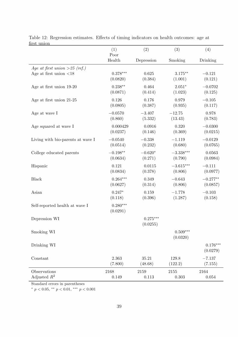
Table 12: Regression estimates. Effects of timing indicators on health outcomes: age atfirst union

(1) (2) (3) (4)Poor


Age at first union >25 (ref.)Age at first union <18 0.378∗∗∗ 0.625 3.175∗∗ −0.121

(0.0820) (0.384) (1.001) (0.121)

Age at first union 19-20 0.238∗∗ 0.464 2.051∗ −0.0702(0.0871) (0.414) (1.023) (0.125)

Age at first union 21-25 0.126 0.176 0.979 −0.105(0.0805) (0.387) (0.935) (0.117)

Age at wave I −0.0570 −3.407 −12.75 0.978(0.860) (5.332) (13.43) (0.783)

Age squared at wave I 0.000429 0.0916 0.320 −0.0300(0.0237) (0.146) (0.369) (0.0215)


College educated parents −0.198∗∗ −0.620∗ −3.338∗∗∗ 0.0563(0.0634) (0.271) (0.790) (0.0984)

Hispanic 0.121 0.0115 −3.615∗∗∗ −0.111(0.0834) (0.378) (0.806) (0.0977)

Black 0.264∗∗∗ 0.349 −0.643 −0.277∗∗

(0.0627) (0.314) (0.806) (0.0857)

Asian 0.247∗ 0.159 −1.778 −0.103(0.118) (0.396) (1.287) (0.158)


(0.0291)


(0.0255)


(0.0320)


(0.0279)

Constant 2.363 35.21 129.8 −7.137(7.800) (48.68) (122.2) (7.155)


39

Table 13: Regression estimates. Effects of timing indicators on health outcomes: age atfirst child

(1) (2) (3) (4)Poor


Age at first children >25 (ref.)Age at first children <18 0.432∗∗∗ 0.771∗ 4.348∗∗∗ 0.223∗

(0.0839) (0.382) (1.060) (0.104)

Age at first children 19-20 0.278∗∗ −0.0794 2.867∗ 0.224(0.0980) (0.411) (1.232) (0.121)

Age at first children 21-25 0.238∗∗ 0.469 1.538 0.0886(0.0808) (0.330) (0.869) (0.0868)

Age at wave I 0.0200 −3.560 −0.921 1.279∗

(0.702) (5.698) (8.631) (0.537)

Age squared at wave I 0.0000226 0.0971 0.00795 −0.0373∗

(0.0196) (0.156) (0.240) (0.0148)

Living with bio-parents at wave I −0.0291 −0.441 −1.997∗∗ 0.00160(0.0606) (0.262) (0.758) (0.0727)

College educated parents −0.215∗∗ −0.677 −3.774∗∗∗ −0.195∗

(0.0761) (0.361) (0.860) (0.0796)

Hispanic −0.0167 −0.380 −4.349∗∗∗ 0.0134(0.0967) (0.425) (0.945) (0.114)

Black 0.0986 0.146 −2.838∗∗ −0.251∗∗

(0.0705) (0.379) (0.931) (0.0849)

Asian 0.353∗ 0.912 −2.027 −0.143(0.179) (0.517) (1.369) (0.171)


(0.0335)


(0.0286)


(0.0368)


(0.0286)

Constant 1.272 36.57 18.58 −10.51∗

(6.309) (52.07) (77.88) (4.892)


40

Table 14: Regression estimates. Effects of quantum indicators on health outcomes: se-quences’ turbulence.

(1) (2) (3) (4)Poor


Turbulence 0.0217 0.0166 0.243∗ 0.000212(0.0114) (0.0326) (0.117) (0.0135)

Age at wave I 0.329 −8.882∗ −30.49∗ 0.562(1.477) (4.495) (15.03) (1.108)

Age squared at wave I −0.0105 0.242 0.806∗ −0.0185(0.0406) (0.124) (0.410) (0.0297)

Living with bio-parents at wave I −0.0752 −0.106 −1.429∗ −0.0103(0.0533) (0.152) (0.649) (0.0722)


Hispanic 0.166 −0.121 −3.680∗∗∗ −0.155(0.0912) (0.238) (0.749) (0.0957)

Black 0.162∗∗ 0.417 −1.134 −0.283∗∗∗

(0.0620) (0.221) (0.783) (0.0809)

Asian 0.190 −0.140 −1.850 −0.107(0.119) (0.244) (1.249) (0.155)


(0.0295)

CES-D scale at wave I 0.229∗∗∗

(0.0254)


(0.0316)


(0.0273)

Constant −0.900 83.55∗ 292.0∗ −3.461(13.43) (40.79) (137.7) (10.32)


41

Figure 3: Average time spent in each state by typology of trajectory

42

family trajectories and health. a life course perspective

Documents