September 16, 2008 The Focus Issue 67

www.padtinc.com 1 1-800-293-PADT

By Rod SchollContinuing from last month’s article <link>we explore the various methods of attachingshell element to solid element regions. Last

time we explored sharing nodes, especiallyusing a “painted-on region” or overlap re-gion to transfer the moments. This ap-proach requires a matched mesh betweenthe shell and solid part, a definite disadvan-tage.

In this article, wewill explore the useof contact elementsand contrast the re-sults with the theo-retical, as well as the“painted-on” ap-proach. We defined

our test case previously, and show a theo-retical equivalent stress of 100 in the shellsat the interface, and 4.00 at the base of thesolid.

Using CONTA17X ElementsThe contact pair will be created by mesh-ing the thin area’s (shell element region)interface nodes with CONTA175s or inter-face lines with CONTA177s, and the solidface(s) with CONTA 170s. When usingthe CONTA17Xs, use Keyoption 12=5,and 2=2. Also, you might specify theSHSD setting, but given that it impacts the

September 15, 2008 A Publication for ANSYS Users Issue 67

By Doug OatisLong has the Workbench community toiledto create 2D geometry from 3D CAD mod-els. Maybe toiled is the wrong word, but itwasn’t something that was considered“pleasant”. In my opinion, it was easier tosetup a 2D analysis in ANSYS PREP7 thanin Simulation…until today!

The requirements for doing a 2D analysis inSimulation are identical to PREP7. Yourgeometry must exist on the XY plane. Ifyou’re doing an axisymmetric problem, thegeometry must also be on the +X side, withyour Y-Axis as the axis of revolution. As

far as I knew, there were two ways to createthis geometry. The first method involvedbeing skilled in whatever CAD package youwere using, creating datum lines, and man-ually building up each area from lines. Thesecond method used DesignModeler toslice/dice the geome-try to ‘expose’ the axi-symmetric face. Youwould then createsketch planes fromeach face, and finallyused ‘Create > Surfacefrom Sketch’ to buildeach 2D body. Thisworked okay, unlessyou had more than ~5 bodies, at which pointyou needed super-ergonomic hardware toprevent permanent ligament damage.

Now, just as Ash realized that by strappinga chain-saw to his arm he could create agreat weapon, I have realized DM has a toolwell suited to simplify and improve thisprocedure. That tool is Thin/Surface. Now,

the typical usage of the Thin/Surface is tohollow out solid bodies. You select thefaces you want to keep/remove, give athickness, and the CAD engine chugs alonguntil it’s hollowed the part out whilekeeping/removing the selected surfaces.

However, if you spec-ify a thickness of 0,and a face offset of 0,it acts as face extrac-tor. If you’re a /prep7user (don’t call it AN-SYS Classic!), this isthe same as deletingall the volumes andareas except for the

selected faces.

So now we have a face-extractor tool, allthat needs to be done is to slice the geome-try to create the faces. This can be donethrough a series of Slices and Body Opera-tion = Delete. Or, you can use ‘Tools >Symmetry’ and select up to three symmetryplanes. The ‘Symmetry’ tool will automat-

Shell To Solid Interfaces:Using Contact

Table of Contents2D Geometry in Design Modeler --------------------------1Shell to Solid Interfaces: Using Contact -----------------1Sail Boat Dagger Board Optimization ---------------------4Awesome APDL: Looping on Tables ---------------------7News and Links ------------------------------------------------7

(Cont. on pg. 2)

(Cont. on pg. 3)

Fast and Easy 2D Geometrywith DesignModeler

September 16, 2008 The Focus Issue 67

www.padtinc.com 2 1-800-293-PADT

generation of the virtual shell elements,this would be more meaningful for a mis-matched mesh.

Lap JointFor comparison with the shell method theresults for a lap joint are shown in Figure 2.The edge contact method is also shownbecause of its characteristic edge effects, inFigures 3 & 4. The results are summarizedin Table 1.

First let’s look at the results of the edgecontact – we see easily that there is a falsestress concentration at the interface in theshell elements. Thus for a lap type joint,it’s hard to recommend this Edge contactapproach.

However, the nodal contact approach, af-fords great accuracy for both the nodalsolution and element solution where we’veseen earlier that the overlapping shell ap-proach (painted-on method) the nodal solu-tion was much less accurate with this mesh.

Down near the base, for this mesh error was3.3% using the painted shells, where thecontact method reduced the error to 1.2%.

Finally, we see at the interface both contactapproaches are non-conservative in the sol-id elements at the interface.

Take away: For lap joints, the nodal con-tact approach is best, remembering that thesolid stresses at the interface are greatlynon-conservative, and must be handled dif-ferently if they drive the design.

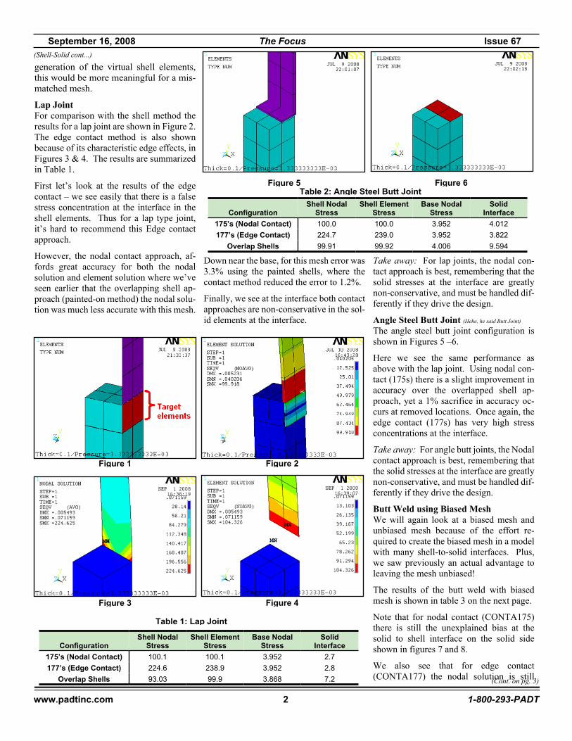
Angle Steel Butt Joint (Hehe, he said Butt Joint)

The angle steel butt joint configuration isshown in Figures 5 –6.

Here we see the same performance asabove with the lap joint. Using nodal con-tact (175s) there is a slight improvement inaccuracy over the overlapped shell ap-proach, yet a 1% sacrifice in accuracy oc-curs at removed locations. Once again, theedge contact (177s) has very high stressconcentrations at the interface.

Take away: For angle butt joints, the Nodalcontact approach is best, remembering thatthe solid stresses at the interface are greatlynon-conservative, and must be handled dif-ferently if they drive the design.

Butt Weld using Biased MeshWe will again look at a biased mesh andunbiased mesh because of the effort re-quired to create the biased mesh in a modelwith many shell-to-solid interfaces. Plus,we saw previously an actual advantage toleaving the mesh unbiased!

The results of the butt weld with biasedmesh is shown in table 3 on the next page.

Note that for nodal contact (CONTA175)there is still the unexplained bias at thesolid to shell interface on the solid sideshown in figures 7 and 8.

We also see that for edge contact(CONTA177) the nodal solution is still

(Shell-Solid cont...)

(Cont. on pg. 3)

ConfigurationShell Nodal

StressShell Element

StressBase Nodal

StressSolid

Interface175’s (Nodal Contact) 100.1 100.1 3.952 2.7177’s (Edge Contact) 224.6 238.9 3.952 2.8

Overlap Shells 93.03 99.9 3.868 7.2

Figure 1 Figure 2

Figure 3 Figure 4

Table 1: Lap Joint

ConfigurationShell Nodal

StressShell Element

StressBase Nodal

StressSolid

Interface175’s (Nodal Contact) 100.0 100.0 3.952 4.012177’s (Edge Contact) 224.7 239.0 3.952 3.822

Overlap Shells 99.91 99.92 4.006 9.594

Figure 5 Figure 6Table 2: Angle Steel Butt Joint

September 16, 2008 The Focus Issue 67

www.padtinc.com 3 1-800-293-PADT

ically cut and remove bodies de-fined by the selected planes. The3D to 2D example shown abovewas actually created with justtwo operations (not including the‘Freeze’). If your planar facesaren’t on the global XY plane,which is the first plane listed inthe model tree, you can use a ‘Body Opera-

tion > Move’ to translatethe faces. Once you’reready, go to the ‘Project’page and set the ‘AnalysisType’ to be 2D (it defaultsto 3D) and then launchSimulation. Finally, setthe planar behavior(axisymmetric, plane

stress, plane strain, etc).

Remember to use this tool wisely…andshop smart, shop S-Mart.

Editor’s note: For those of you who are tryingto figure out who Ash is and if S-Mart is a typo,Doug is trying to impress you all by referencinga cult classic movie. I had to look it up. He istalking about “Army of Darkness” a cult over-the-top horror spoof film by Sam Raimi, thesame guy who brought us Xena and more recent-ly, Spiderman.

(2D DM cont...)

quite off, but for this biased mesh, so is theelement solution!

Take away: We are left to conclude, that ifone must have a biased mesh at a butt weldlocation between shell and solids, the bestof the above approaches is to tie into the topsurface either with overlapping shells, orwith nodal contact (CONTA175). Theoverlapping shell method requires one torely on element results (rather than nodal).The nodal contact method requires oneoverlook the unexplained bias at the inter-face, although the peak is close in magni-tude to expected stresses. Given ourhesitancy to believe much about actualstresses at such an interface, this is probablypalatable.

Butt Weld – Unbiased MeshGiven the results above with the unbiasedmesh, and considering that we discoveredwith overlapping shells the most accuracywas obtained by not biasing the mesh for abutt weld, let’s look at what results areobtained with an unbiased mesh using con-tact methodology. In most cases biasing themesh is extra work, so it’s reasonable tohope that the following exploration illumi-nates a clear winner. The results of the buttweld with unbiased mesh is shown in table4.

Once again, we see that the two best meth-ods are overlapping shells on the top sur-face, or nodal contact (CONTA175) on thetop surface. Here, however, with the unbi-ased mesh and contact approach, we findthat the removed location of the base, has a1% error or so… not a big deal, but notablefor such a removed location. Also, theoverlapping shells on top surface approachnow has nodal stress results in the shellregion which are quite accurate! So itseems that for both overlapping shells, andthe contact approach, biasing the mesh isstill not greatly advantageous.

Take Away: In a knock-down drag out fight,for the butt weld, I have to side with theoverlapping shells on the top surface, ratherthan contact technology (CONTA17X) be-cause of the better stress results at removedlocations, and higher (more accurate) stress

in the solid region near the shell to solidinterface (although still quite non-conserva-tive). With either approach, we can likelybreath a sigh of relief in that there isn’t adistinct advantage in biasing the mesh tomatch the shell thickness at the interface.

Table 3: Butt Weld with Biased Mesh

Figure 8Figure 7

ConfigurationIncludedSurfaces

ShellStress(Nodal)

ShellStress

(Element)

BaseStress(Nodal)

SolidInterfaceStress

(Element)175s (Nodal Contact) Top 100.8 100.8 4.005 39.60175s (Nodal Contact) Side 100.0 100.1 4.005 2.540175s (Nodal Contact) Top & Side 100.0 100.1 4.005 2.410177s (Edge Contact) Top 224.0 239.6 4.005 39.81177s (Edge Contact) Side 224.6 238.9 4.005 3.290177s (Edge Contact) Top & Side 224.6 238.9 4.005 3.200

Overlap Shells Top 86.14 106.4 4.005 33.310Overlap Shells Side 86.14 99.92 4.005 10.110Overlap Shells Top & Side 86.14 99.92 4.005 11.940

Table 4: Butt Weld with Un-Biased Mesh

ConfigurationIncludedSurfaces

ShellStress(Nodal)

ShellStress

(Element)

BaseStress(Nodal)

SolidInterfaceStress

(Element)175s (Nodal Contact) Top 100.0 100.0 3.952 4.010175s (Nodal Contact) Side 100.1 100.1 3.952 2.700175s (Nodal Contact) Top & Side 100.0 100.0 3.952 1.590177s (Edge Contact) Top 224.7 239.0 3.952 3.820177s (Edge Contact) Side 224.6 238.9 3.952 2.800177s (Edge Contact) Top & Side 224.6 239.0 3.952 1.690

Overlap Shells Top 99.92 99.92 4.006 9.590Overlap Shells Side 93.03 99.92 3.868 7.240Overlap Shells Top & Side 99.92 99.92 4.006 4.130

(Shell to Solid cont...)

September 16, 2008 The Focus Issue 67

www.padtinc.com 4 1-800-293-PADT

By Ted HarrisAn old sailing jokesays that a sailor was

sailing across the bay, when a power boater zoomed in alongside. The power boater yelled, "I'll race you there!" Thesailor replied, "I am already there."

I am nowhere near an expert on sailing, on sail boat design, or evenon optimization technology. However, because I enjoy sailing aswell as learning how to do new things with ANSYS, Inc. products,I decided that I would combine those activities and try out anoptimization on a small sail boat dagger board taking advantage ofthe link that exists between CFX and DesignXplorer at version11.0. This endeavor resulted in a paper I presented at the recent2008 ANSYS User Conference in Pittsburgh. The following is anarticle discussing the process.

First, a few definitions that are relevant to the project.

Dagger Board - a keel that slides in and out of a slot on a sailboat. It is removed in shallow water, for transport, and storageand is dropped in place when under sail. It serves as a second'airfoil' (the sail being the first) under the water to prevent theboat from moving sideways while under sail. Figure 1 showsthe original dagger board from my boat

Reaching - sailing perpendicular to the wind, which is typicallythe fastest way to sail in a small boat. 'Lift' created on the sailin this configuration pulls the boat in the forward direction.

CFX - one of ANSYS, Inc.'s two current CFD tools (the otherbeing FLUENT). CFX can run as a module within ANSYSWorkbench.

DesignXplorer - the ANSYS Workbench design optimization,DFSS, and robust design tool.

DesignModeler - the ANSYS Workbench geometry creationand modification tool.

Since there was not a large amount of time or resources to completethe project, some assumptions were made to reduce the scope of theproblem while still hopefully demonstrate the techniques involved.First, it was decided that the goal would be a geometric optimiza-tion of the dagger board to increase the tangential force on theboard during sailing at a reach, with the goal of increasing thespeed at which one can sail with a cross wind. It was thought thatthis would allow for greater resistance to side slip and hence fasterforward speed.

Next, the effects of the sail, rigging, rudder, waves, etc. wereignored. It was assumed that the boat was moving on smooth waterat 7 knots at a constant orientation. Only steady-state conditionswere modeled.

Only one configuration of the board in the water was considered,15° roll from vertical and 10° rotation from the flow direction. TheDesignModeler model had those angles parameterized so otherconfigurations could be easily considered in any future runs.Fillets on the board were removed for the optimization study, but adetailed model with the fillets and a much finer mesh was analyzedin CFX for the optimized configuration to confirm the trends.

No check of drag in the direction of travel was considered, but thiscould be added in future studies as well as creating a much moredetailed objective function, rather than the fairly simplistic maxi-mization of side force on the board.

The optimization process is shown in figure 2:

The optimization process started with geometry definition inDesignModeler. Since the dagger board must fit in a slot in thehull, the shape was assumed to remain as a ¾ in. thick wood plank.Therefore 2D parametric geometry was defined and extruded ¾ in.into 3D to define the board. The shape was allowed to changewithin the 2D plane. Seven geometric input parameters were cho-sen to participate in the optimization. Also, instead of sliding downfrom the top of the boat, it was conceded that an optimized shape

ANSYS on the LakeAn Optimization of a Sail Boat

Dagger Board using DesignXplorer

(Cont. on pg. 5

September 16, 2008 The Focus Issue 67

www.padtinc.com 5 1-800-293-PADT

would likely need to slide up from under the water into the slot inthe hull, necessitating a re-movable attachment sys-tem.

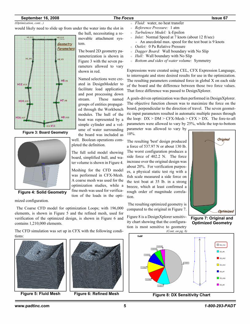
The board 2D geometry pa-rameterization is shown inFigure 3 with the seven pa-rameters allowed to varyshown in red.

Named selections were cre-ated in DesignModeler tofacilitate load applicationand post processing downstream. These namedgroups of entities propagat-ed through the Workbenchmodules. The hull of theboat was represented by asimple cylinder and a vol-ume of water surroundingthe board was included as

well. Boolean operations com-pleted the definition.

The full solid model showingboard, simplified hull, and wa-ter volume is shown in Figure 4.

Meshing for the CFD modelwas performed in CFX-Mesh.A coarse mesh was used for theoptimization studies, while afine mesh was used for verifica-tion of the loads in the opti-

mized configuration.

The Coarse CFD model for optimization Loops; with 196,000elements, is shown in Figure 5 and the refined mesh, used forverification of the optimized design, is shown in Figure 6 andcontains 1,210,000 elements.

The CFD simulation was set up in CFX with the following condi-tions:

○ Fluid: water, no heat transfer○ Reference Pressure: 1 atm○ Turbulence Model: k-Epsilon○ Inlet: Normal Speed at 7 knots (about 12 ft/sec)

- An anecdotal max. speed for the test boat is 9 knots○ Outlet: 0 Pa Relative Pressure○ Dagger Board: Wall boundary with No Slip○ Hull: Wall boundary with No Slip○ Bottom and sides of water volume: Symmetry

Expressions were created using CEL, CFX Expression Language,to interrogate and store desired results for use in the optimization.The resulting parameters contained force in global X on each sideof the board and the difference between those two force values.That force difference was passed to DesignXplorer.

A goals-driven optimization was then performed in DesignXplorer.The objective function chosen was to maximize the force on theboard, perpendicular to the direction of travel. The seven geomet-ric input parameters resulted in automatic multiple passes throughthe loop: DX > DM > CFX-Mesh > CFX > DX. The fore-to-aftparameters were allowed to vary by 25%, while the top-to-bottomparameter was allowed to vary by10%.

The resulting 'best' design produceda force of 537.97 N or about 130 lb.The worst configuration produces aside force of 402.2 N. The forceincrease over the original design wasabout 20%. For verification purpos-es, a physical static test rig with afish scale measured a side force onthe test boat at 35 lb. in a strongbreeze, which at least confirmed arough order of magnitude correla-tion.

The resulting optimized geometry iscompared to the original in Figure 7.

Figure 8 is a DesignXplorer sensitiv-ity chart showing that the configura-tion is most sensitive to geometry

H2,0.0

H2,V3

H5,V6

H7,V8

H9,V10

0.0,V11

H16,V17

H14,V15

H12,V13

H1,V4

H1,0.0

Figure 3: Board Geometry

Figure 4: Solid Geometry

Figure 5: Fluid Mesh Figure 6: Refined Mesh

Figure 7: Original andOptimized Geometry

Figure 8: DX Sensitivity Chart

(Cont. on pg. 6)

(Optimization, cont...)

September 16, 2008 The Focus Issue 67

www.padtinc.com 6 1-800-293-PADT

parameter DS_V11. This is the length (depth) of the middle of theend of the board.

Figure 9 shows the resulting CFX Pressure distribution for theoptimized shape and Figure 10 shows the water streamlines for thesame case.

Structural runs were per-formed in Workbench Sim-ulation to compare thedeflections of the originalboard vs. the optimizedboard for their respectivepressure loadings. The pre-dicted tip deflection of theoptimized board was slight-ly higher than the original.Figure 11 shows the deflec-tion results from Simula-tion.

With the optimized shapeobtained from theDesignXplorer/CFX pro-cess, the next step was tofabricate a board for testingpurposes. The author con-structed the optimized board from a plank of poplar. Poplar waschosen over oak because it was less expensive and a bit easier towork with. Figure 12 shows the Prototype

The two boards and an Alcort Minifish sail boat were then taken toa local lake to obtain experimental results. Back to back runs weremade with the original dagger board and the optimized board.Time constraints limited the testing to one pass with each board.Each pass was about 0.85 mile round trip. The maximum speed foreach run was stored using a hand-held GPS receiver. Although theboat 'seemed' faster with the optimized board, the max speedrecorded was 7.5 mph, vs. 7.6 mph with the original board (about6.5 knots, not too far off the assumption in the CFD runs of 7.0knots). Since wind conditions vary constantly the results havebeen deemed inconclusive, although the boat did seem to handlebetter with the optimized board.

In conclusion, CFX linked with DesignXplorer can be used as atool to find an optimal design for a well-defined problem. Moredetails would be needed to really hone the technique for thisproblem, such as using a more detailed objective function, furtherstudying mesh density effects, including fillets in each pass, utiliz-ing other configurations of the angles of the boat and board as wellas velocity, and greater potential geometry variations.

Figure 9: CFX Pressure Distribution

Figure 10: CFX Streamlines

Figure 11: Structural Deflection

Figure 12: Making the Prototype

Figure 13: The Author Testing the Designon a Nice Windy Day

(Optimization, cont...)

September 16, 2008 The Focus Issue 67

www.padtinc.com 7 1-800-293-PADT

Let’s say you want to apply a surface load or boundary force(SF/BF) to a bunch of areas. But you don’t know how many tablesor areas you are going to have. So you make a component/nameselection for each zone you want your load on and number themsequentially (myzone_1, myzone_2, etc...) and then you make atable for each zone (mytbl_1, mytbl_2, etc...) Then you make a doloop that selects each component followed by an SF or BF toassign to assign the load:*do,I,1,3 cmsel,s,myzone_%i% bf,all,hgen,mytbl_%i%*enddo

This is especially useful when you are writing APDL snippets aWorkbench Simulation model. If you number hour named selec-tion you can have a very general macro that goes through andsemi-automatically applies the proper loads. Sounds good so far.

But, and there is always a but, if you try the above code you willfind out that the BF command is applying a value of0.7888609052E-30. This is because the parser only treats a textstring as a table name if it starts and stops with a percent sign.Anything other than that and ANSYS thinks you are putting in aparameter and not a table name. If you try %mytbl_%%i% you get anerror. And doing atmp = mytbl_%i% and specify %atmp% does notwork either, because it looks for a table called atmp.

So, enter the old “self generating macro” approach: have yourmacro write the proper command to a file, then read that file. Theexample example given here is even more general, in that the tableand component names are variables as well. It was used as a wayto apply a series of tables that vary by X position under fourdifferent coordinate systems.

Near the bottom you will find the CFOPEN, VWRITE, CFCLOS,/INPUT, /DELETE needed to build and execute a command on thefly that can be used with whatever application you want to use iton.*do,i,1,4 *DEL,_FNCNAME ! clean up variables *DEL,_FNCMTID *DEL,_FNCCSYS *SET,_FNCNAME,'d_test%i%' !define name of table *SET,_FNCCSYS,act_csys !set csys for the table! Define Table: *DIM,%_FNCNAME%,TABLE,6,12,1,,,,%_FNCCSYS%! Build table: *SET,%_FNCNAME%(0,0,1), 0.0, -999! SNIP - lines removed to conserve space *SET,%_FNCNAME%(0,6,1), 0.0, -2, 0, 1, 2, 17, -1 *SET,%_FNCNAME%(0,12,1), 0.0, 99, 0, 1, -3, 0, 0 cmsel,s,%d_root%%i% ! select named selection/group d_a='%'! Put percent sign in a variable *cfopen,d_temp,txt !open a temp file to write to *vwrite,d_a,_FNCNAME,d_a ! Write the command bf,all,hgen,%C%C%C *cfclose ! Close the file /input,d_temp,txt ! read in the command /delete,d_temp,txt ! Clean up after yourself act_csys=act_csys+1 !increment your csys*enddo

One key thing you will notice, is that you create a charactervariable to hold your percent signs (d_a) because the *vwritecommand treats %’s as special characters. Another way to do itwould be to put double %%’s on the format line:*vwrite,_FNCNAME ! Write the commandbf,all,hgen,%%%C%%.

News - Links - Info· XANSYS now has a blog for opinion, observations

and some humor <xansys.blogspot.com>

· Ansoft Acquisition is Completed <link>

· The channel partner in Italy, Enginesoft has anawesome Newsletter (makes ours look amateur).Many of the articles are in english: <link>

· Get ANSYS news directly by subscribing to theirRSS feed: <link>

· While looking at the Enginsoft newsletter, youshould check out their optimization tool: ModeFron-tier: <link>

The Focus is a periodic publication of Phoenix Analysis & Design Technologies (PADT). Its goal is to educate and entertain the worldwide AN-SYS user community. More information on this publication can be found at: http://www.padtinc.com/epubs/focus/about

Looping on Numbered TablesAwesomeAPDL

Upcoming Training ClassesMonth Start End # Title LocationSep '08 9/18 9/20 102 Introduction to ANSYS, Part II Tempe, AZ

9/22 9/23 201 Basic Structural Nonlinearities Tempe, AZ9/24 9/25 204 Advanced Contact and Fasteners Tempe, AZ

Oct '08 10/2 10/3 104 Workbench Simulation – Intro Las Veg., NV10/6 10/7 205 Workbench Simulation Dynamics Tempe, AZ10/9 10/10 100 Engineering with FE Analysis Tempe, AZ

10/14 10/15 207 WB Simulation:Struct. Nonlinearities Tempe, AZ10/16 10/17 302 Workbench Simulation Heat Transfer Tempe, AZ10/20 10/20 107 ANSYS Workbench DesignModeler Tempe, AZ10/22 10/24 902 Multiphysics Simulation for MEMS Tempe, AZ10/27 10/27 411 WB Simulation Electromagnetics Tempe, AZ10/28 10/28 206 WB Rigid & Flexible Dynamics Tempe, AZ

Nov '08 11/5 11/7 101 Introduction to ANSYS, Part I Tempe, AZ11/10 11/10 702 ANSYS Workbench DesignXplorer Tempe, AZ11/12 11/13 301 Heat Transfer Tempe, AZ

11/17 11/18 102 Introduction to ANSYS, Part II Tempe, AZ11/19 11/20 204 Advanced Contact and Fasteners Tempe, AZ11/24 11/25 604 Introduction to CFX Tempe, AZ

September 16, 2008 The Focus Issue 67

www.padtinc.com 8 1-800-293-PADT

F o r o v e r a d e c a d e A N S Y S u s e r s a r o u n d t h e

w o r l d h a v e b e e n g a t h e r i n g o n t h e X A N S Y S

m a i l i n g l i s t t o s h a r e t h e i r k n o w l e d g e ,

e x p e r i e n c e a n d h u m o r . J o i n t h e c o n v e r s a t i o n

w i t h 3 , 5 0 0 + p r a c t i t i o n e r s o n t h e l a r g e s t

i n d e p e n d e n t A N S Y S c o m m u n i t y o n t h e w e b .

www.xansys.org

ANSYS + MathcadPADT is Taking the Lead

� Mathcad Sales and Support toANSYS users

� Development of Opensourceinterface tools

� Training and educational materials

� Stay tuned to “The Focus” to learnmore