fast and high quality fusion of depth maps...fast and high quality fusion of depth maps christopher...

Fast and High Quality Fusion of Depth Maps

Christopher ZachDepartment of Computer Science

University of North Carolina at Chapel Hill

Abstract

Reconstructing the 3D surface from a set of providedrange images – acquired by active or passive sensors – isan important step to generate faithful virtual models of realobjects or environments. Since several approaches for highquality fusion of range images are already known, the run-time efficiency of the respective methods are of increasedinterest. In this paper we propose a highly efficient methodfor range image fusion resulting in very accurate 3D mod-els. We employ a variational formulation for the surfacereconstruction task. The global optimal solution can befound by gradient descent due to the convexity of the under-lying energy functional. Further, the gradient descent pro-cedure can be parallelized, and consequently acceleratedby graphics processing units. The quality and runtime per-formance of the proposed method is demonstrated on well-known multi-view stereo benchmark datasets.

1. Introduction

The generation of high-quality, dense geometric mod-els from passive or active sensors is still an active researchtopic. There is a large amount of research devoted to thetask of surface reconstruction from a sparse or semi-denseset of given 3D points. In order to handle meshes witharbitrary genus, a volumetric representation is often uti-lized as the underlying data structure. Voronoi cells are thebasis for some geometric methods for surface reconstruc-tion [2, 1]. Regular volumetric grids are far more commonfor this purpose. Level set approaches [30, 29] fall into thiscategory, although they are conceptually different than theapproaches discussed next. To our knowledge none of theseyet mentioned methods was employed on larger scale real-world data sets potentially containing a substantial amountof noise and outliers.

With the increased availabilty of laser scanning devicesenabling dense measurements of real-world surfaces, sev-eral methods were developed to create full 3D models fromsuch 2.5D range data. An explicit polygonal approach tomerge several range images is described in [22].

Early range image fusion methods incorporating a reg-ular voxel space include Curless and Levoy [8], Hilton etal. [10] and Wheeler et al. [24]. These methods initiallycompute a signed distance function for the final surface byaveraging the distance fields induced by the given rangeimages. The boundary representation of the resulting sur-face is obtained by an isosurface polygonization method.The merged distance field is computed separately on vox-els, which allows those methods to be efficient, but spatialcoherence and smoothness of the resulting mesh cannot beenforced. Volumetric graph cuts for computer vision [23]allow the incorporation of surface regularization into thevolumetric fusion framework. Hornung and Kobbelt [12]present a general surface reconstruction method for sparseand dense input point clouds. Since their approach is basedon a geodesic problem formulation, a constrained optimiza-tion scheme using conservative interior/exterior estimates isrequired to avoid degenerate solutions. Other recent workon volumetric surface reconstruction [13, 14] directly esti-mates the corresponding characteristic function from (ori-ented) point samples. Lempitsky and Boykov [15] presenta global shape fitting method, that shares several elementswith our approach (see the TV-Flux method described inSection 2), but involves a sophisticated graph cut procedurefor discrete optimization.

Finally, several methods attempt to reconstruct an objectsurface directly from captured image data, thereby avoid-ing the use of active sensors. Such multi-view stereo ap-proaches enable a convenient procedure for 3D reconstruc-tion, and allow the creation of virtual representations on alarger scale. An important group of methods estimates theobject surface directly from a consistency score for voxels(most notably, a photo-consistency measure [19, 26, 23, 21,11, 3, 4]). Other approaches compute intermediate depthmaps from small-baseline stereo in the first instance anduse multiple depth images to perform a final surface in-tegration step. Strecha et al. [20] and Merrell et al. [16]clean the initially obtained depth maps by fusing informa-tion from neighboring views. The latter work is targeted onreal-time large scale reconstruction, hence runtime perfor-mance was considered more important than the final mesh

Proceedings of 3DPVT'08 - the Fourth International Symposium on 3D Data Processing, Visualization and Transmission

June 18 - 20, 2008, Georgia Institute of Technology, Atlanta, GA, USA

quality. Up to now [16] was the only reported approachto generate dense 3D geometry in less than one minute forbenchmark datasets [18].

The method proposed in this work is an approach forgeneral range image integration based on total variationshape denoising. It can be easily extended to a surfacereconstruction procedure for sparse oriented point clouds.Since the main application of our work is object reconstruc-tion from multiple views, we focus on captured images aug-mented with calibration and orientation information as theprimary input data. Depth maps can be obtained by small-baseline stereo methods from image data. Depending onthe image content and on the utilized dense stereo method,the resulting depth maps may contain a substantial amountof outliers and (usually non-Gaussian) noise. Thus, high-quality generation of full 3D models from depth maps isonly possible with a robust approach.

This work extends the approach presented in [27] is sev-eral aspects: first, the distance based data fidelity term pro-posed in [27] is replaced by an histogram based one, al-lowing the whole procedure to be accelerated by moderngraphics processing units. Further, a visual comparison ofthe proposed approach with a continuous formulation of theglobal shape fitting energy [15] is provided. Finally, resultsand runtimes for the large evaluation datasets [18] are pre-sented.

2. Accelerated Range Image Fusion

The input of the main method is a set of potentiallynoisy range images. For best runtime performance, we em-ploy a GPU-based implementation of a plane-sweep stereomethod [25, 7, 28] to obtain these initial depth maps. Sincethis method is a purely local approach to dense stereo, onecan expect a substantial amount of noise and mismatchesin the resulting depth images. This set of depth maps pro-vides 2.5D geometry for each view, which are subsequentlyconverted to truncated signed distance fields (denoted byfi : Ω → R for a voxel space Ω). We use a simple z-comparison to obtain a fast and suitable approximation ofthe true distances.

In [27] the implicit representation of the final surface isobtained as the spatially regularized median of the provided3D distance transforms, i.e. a TV-L1 energy consisting of atotal variation part,

∫|∇u|d~x =

∫‖∇u‖2d~x, and an L1 (i.e.

absolute differences) term,

ETV−L1(u) =

∫Ω

|∇u|+ λ

∑i

|u− fi|

d~x, (1)

is minimized with respect to u for the given set of distancetransforms fi. The resulting function u : Ω → R is thesigned distance to the fused model, and the corresponding

surface representation can be extracted by any isosurfacepolygonization method. The optimization procedure pre-sented in [27] is efficient and globally optimal, but not par-ticularly suited to be accelerated by a GPU. Specifically,the generalized thresholding procedure described in Propo-sition 2 in [27] requires a varying amount of computationfor each voxel, which typically yields to a suboptimal per-formance on GPUs.

In this work we modify the TV-L1 approach in two as-pects: first, the data fidelity

∑i |u−fi| is replaced by a more

GPU-friendly approximation using weighted distances toevenly spaced representative values cj ; and second, the ex-pensive generalized thresholding step performing an opti-mal line search is replaced by a simpler and faster descentstep.

We assume that the provided distance fields fi arebounded to the interval [−1, 1]. Hence we sample this in-terval by evenly spaced bin centers cj , and approximate theoriginal data fidelity term

∑i |u − fi| by

∑j nj |u − cj |,

where and nj are the respective frequencies. Thus, fi is re-placed by its closest bin center cj in the data fidelity term.Note that the data term is integrated over the voxel space,hence a histogram is maintained for each voxel.

In contrast to the original TV-L1 formulation those fre-quencies can be weighted arbitrarily. Particularly, this al-lows us to reduce the influence of depth values errorneouslyreported behind the true surface. Section 4 illustrates theimpact of this modification. The overall energy to be mini-mized is then

ETV−Hist(u) =∫

Ω

|∇u|+ λ

∑j

nj |u− cj |

d~x. (2)

Analogous to the procedure derived in [27], EHist is re-placed by the strictly convex relaxation

ETV−Histθ (u, v) =

∫Ω

|∇u|+ 1

2θ(u− v)2

+ λ∑

j

nj |v − cj |

d~x, (3)

for a small value of θ. Since this energy functional is(strictly) convex in u and v, a global minimizer can be de-termined by alternating optimization with respect to u andv. Reducing the energy with respect to u and fixed v canbe performed e.g. by Chambolles method [5]. We brieflyreview this method, which provides a global minimizer forthe Rudin-Osher-Fatemi energy [17],

EROFθ (u; v) =

∫Ω

|∇u|+ 1

2θ(u− v)2

d~x. (4)

Note, that we omitted the histogram term, since it does notdepend on u and therefore has a constant value. |∇u| can



be rewritten as

|∇u| = max~p:|~p|≤1

〈~p,∇u〉. (5)

Plugging Eq. 5 into the ROF energy (Eq. 4), and after com-puting the functional derivatives wrt. u and ~p, we obtain thefollowing conditions for stationary points:

∂EROFθ

∂u=

1θ(u− v)−∇ · ~p != 0, i.e. (6)

u = v + θ(∇ · ~p), and (7)∂EROF

θ

∂~p= ∇u + α~p

!= 0. (8)

We employ a gradient descent/projection approach [6],hence |~p| ≤ 1 is enforced after the gradient descent stepand we can omit the Lagrange multiplier α.

The minimization of EHistθ with respect to v is equiva-

lent to (note that we can ignore the constant total variationterm now)

minv

∫Ω

12θ

(u− v)2 + λ∑

j

nj |v − cj |

d~x. (9)

We can carry out this minimization point-wise, since thisenergy does not depend on any derivative of v. Without lossof generality (and omitting the dependence on the currentvoxel ~x), if u ∈ (ck, ck+1) and the stationary point

v∗ = u + λθ

∑j>k

nj −∑j≤k

nj

(10)

is in (ck, ck+1), then v∗ is the minimum argument. Ifv∗ ≤ ck, then v = ck − ε lowers the energy in Eq. 9 fora sufficiently small ε (although it is not a global minimumin general). We exclude the bin centers cj as feasible valuesfor v in order to avoid handling of special cases in the GPUimplementation. If v∗ ≥ ck+1, we choose v = ck+1 + ε.In those (very rare) situations, when cj is exactly the opti-mum, v will oscillate with the values cj±ε. Altogether, thegeneralized thresholding step to determine v for a given uto reduce the energy in Eq. 9 reads as

v = maxck − ε, minck+1 + ε, v∗ (11)

with v∗ defined in Eq. 10 and u ∈ (ck, ck+1).These alternating descent steps to update u and v, re-

spectively, can be efficiently performed on modern GPUs.We employ 8 bins with bin centers cj = 2j/7 − 1 forj ∈ 0, . . . , 7, and the frequencies nj are determined bysimple voting for the closest bin center. We will denote thisprocedure as the TV-Hist approach.

Another method that can be accelerated by GPUsis the global shape fitting approach of Lempitsky and

Boykov [15]. Their energy minimization is based on dis-crete graph cuts, which is hard to parallelize. The utilizedsurface regularization energy is exactly equivalent to totalvariation regularization for binary functions. The data fi-delity term is a flux energy derived from the provided input,a set of oriented, optionally sparse 3D points. Formulatingthese terms in a continuous setting, one arrives at the fol-lowing resulting energy to be minimized:

EFlux(u) =∫

Ω

|∇u|+ λ(∇ · ~f) · u

d~x. (12)

We just remark that (depending on the sign convention) theinput scalar field ∇ · ~f (divergence of the vector field ~f )has positive values inside the presumed surface and negativevalues outside. We refer to [15] for more details. We willcall this approach the TV-Flux method. As for the TV-Histapproach, a simple and efficient procedure to minimize theenergy in Eq. 12 can be specified. It will be demonstrated inSection 4 that the resulting surfaces still contain substantialaliasing artefacts. This is due to the binary characteristics ofthe flux-based data term, since regions with non-vanishingflux strongly “push” to +1 or −1.

3. Implementation

In this section we briefly sketch our implementation ofboth approaches, TV-Hist and TV-Flux, on the GPU usingOpenGL and Cg shader programs. Although the CUDAframework is a new and powerful GPU programming ap-proach, traditional shader programming using OpenGL hasstill some benefits like more mature (and optimized) driversand cached writes to render targets.

At first the input depth maps are converted to a volumet-ric data structure. For every voxel, an (approximate) signeddistance to the surfaces induced by the depth maps is com-puted. This value is clamped to a user-supplied thresholdand scaled to the interval [−1, 1]. We refer to [8, 27] formore details on depth map to volume conversion.

In the TV-Hist approach each voxel holds a histogramcomprised of 10 bins. 8 bins are used to represent the dis-tribution of values in the interior of the interval (−1, 1), i.e.voxels close to the supposed surface. Two separate binsare reserved for values indicating a larger distance to thesurface, one bin counts (scaled) distances smaller or equal-1 (occluded voxel) and one bin represents values greateror equal 1 (empty voxel). The total number of histogramcounts is limited by the number of provided depth maps.In practice, the accumulated count is much smaller, sincea specific voxel is typically only close to a depth surfacefor a subset of views. Thus, allocation of one byte for eachhistogram bin is sufficient.

We use the commonly employed flat layout of 3D vol-umes by mapping the z-slices to rectangular sections in a



2D texture. With a limit of 4096×4096 for the maximumtexture size, voxel spaces slightly smaller than 2563 can behandled (since we incorporate border pixels for the bound-ary conditions). Newer graphics hardware has a 8192×8192limit enabling approximately 4003 voxels. The memory re-quirements are far more constraining: for each voxel, thefollowing data needs to be maintained:

1. 10 bytes for the input histogram,

2. 4 bytes for the current value of u (one float packed infour 8-bit values),

3. 6 bytes are required for the dual variable ~p, since ~p is3-dimensional. A 16-bit floating point representationfor the elements of ~p is sufficient.

In total, the memory footprint of a voxel is 20 bytes (plussome additional buffers in the size of one slice). Thus, a2563 voxel space needs about 320Mb memory on the GPU.The memory requirement for the TV-Flux approach is 12bytes per voxel.

Both methods, TV-Hist and TV-Flux, perform the fol-lowing two alternating steps in the n-th iteration:

1. Update ~p using a gradient descent/projection approach(recall Eq. 8, ∂E/∂~p = ∇u), i.e.

~q ← ~p(n) +τ

θ∇u (13)

~p(n+1) ← ~q/max1, |~q|

. (14)

τ < 1/6 is the timestep of the gradient descent step.

2. Update u via intermediate computation of v. Herewe provide a straightforward procedure to compute v∗

(Eq. 10) suited for stream computing. For the TV-Histapproach, it consists of the following steps:

(a) Compute a boolean (0/1) vector l by component-wise comparison,

l← u(n) > (cj)j=0,1,...,N ,

where cj is the center of bin j (c0 = −∞). N isthe total number of bins.

(b) Compute a similar boolean vector

r ← u(n) < (cj)j=1,...,N+1,

with cN+1 = +∞. The element-wise prod-uct (l · r)j is then the indicator function u(n) ∈(cj , cj+1).

(c) Compute v∗ ← u(n) + λθ 〈r − l, (nj)j〉, where(nj)j is the histogram frequency vector.

(d) Clamp v∗: Compute the interval borders

ck ← 〈l · r, (cj)j=0,1,...,N 〉

andck+1 ← 〈l · r, (cj)j=1,...,N+1〉.

Then v ← maxck − ε, minck+1 + ε, v∗.(e) Finally, u(n+1) ← v + θ(∇ · ~p) (Eq. 7).

Note that this algorithm is already presented in a GPU-friendly manner, since it is based mainly on dot prod-uct and element-wise product calculations. The proce-dure to update u in the TV-Flux approach (Eq. 12) issimpler:

(a) Compute the intermediate value v from

v ← u(n) − λθ(∇ · f).

(b) The new value for u is given by

u(n+1) ← v + θ(∇ · ~p).

These two steps to update ~p and u, respectively, can bemapped directly to correponding fragment programs. Sinceread/write access to the same texture buffer has undefinedbehaviour, the update procedures iterate over the slices ofthe voxel space using an additional temporary buffer. Notethat the gradient and divergence computations must be mu-tually dual, i.e. if forward differences are used to determine∇u, then∇· ~p needs to be computed from backward differ-ences [5].

Both methods are still mostly bandwidth-limited, sincegradient and divergence computations require sampling ofseveral neighboring values. Hence the arithmetic intensityis not very high, and the simpler TV-Flux approach is inpractice only slightly faster than the more complex TV-Histmethod.

We want to point out that these schemata are embeddedinto a coarse-to-fine approach to obtain faster fill-in in re-gions with empty histograms (i.e. voxels distant to any sur-face induced by the depth maps).

4. Results

We show results on two datasets provided for bench-marking multi-view reconstruction methods [18] (see alsovision.middlebury.edu/mview/). The advantageof demonstrating results on these datasets is, that the groundtruth laser-scanned 3D geometry is known and the qualityof obtained dense meshes can be evaluated.

We selected the full and the medium size data sets, called“Temple” (312 images), “Dino” (363 images), “Temple



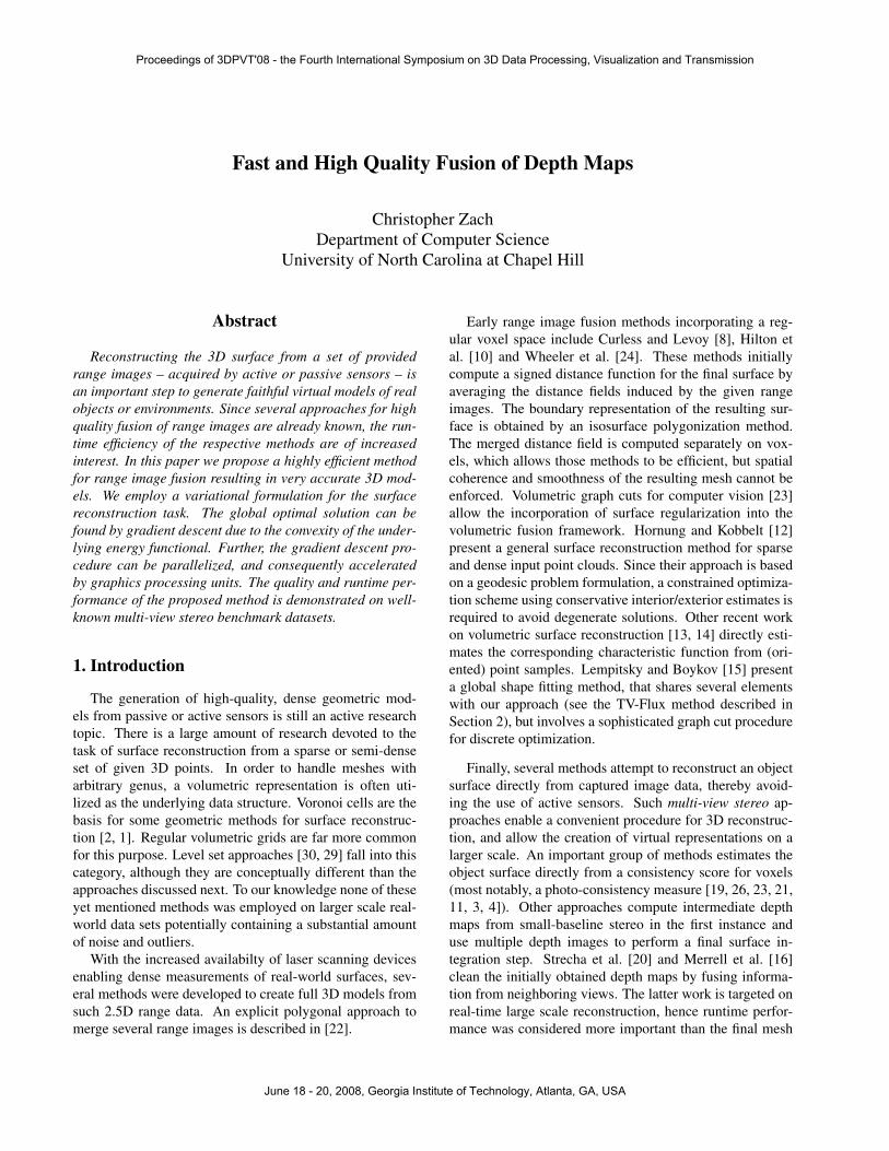
(a) Temple ring depth #1 (b) Temple ring depth #2 (c) Dino ring depth #1 (d) Dino ring depth #2

Figure 1. Selected input depth maps used for later volumetric fusion. The depth maps are not veryclean and contain a certain amount of mismatches.

ring” (47 images) and “Dino ring” (48 images). The re-spective images with a resolution of 640×480 are acquiredin a controlled indoor environment, hence a simple and effi-cient SAD matching cost is sufficient to determine the inputdepth maps. 400 tentative depth planes are evaluated fordense stereo computation. The dark background pixels ofthe captured scene are removed by thresholding the inten-sity values. Pixels with a brightness value of at least 10 areconsidered to be foreground/object pixels, and backgroundpixels otherwise. Figure 1(a)–(d) show a few samples ofthe depth maps obtained by a simple plane-sweep approachusing a 3×3 SAD correlation window and two neighboringviews as moving (warped) images.

Table 1 summarizes the characteristic numbers of thesedatasets, and depicts the runtimes observed to generate theintermediate depth maps and the fused 3D model, respec-tively. We further quote the runtimes for the actual (pureCPU-based) integration step from [27], where available.All timings are measured on PC hardware equipped witha NVidia GeForce 8800 Ultra GPU. Additionally, the accu-racy results according to the main table of the Middleburymulti-view stereo page are displayed, too.

The surface meshes for both “ring” datasets are obtainedwith a value of λ equal to 0.08. The value of λ for the fulldatasets is scaled according to the number of images, i.e.λ = 0.08 47

312 for the full “Temple” dataset. θ is always setto 0.02, and in practice, the exact value of θ is not criti-cal. The timestep τ is fixed to 0.16. We use three levels forthe multi-scale pyramid, and 120 iterations are performedon every level. Although the energy has still not convergedafter this number of iterations, the extracted isosurfaces re-main virtually constant. Figure 2(a)–(d) depict the obtainedmeshes for the “Temple” and “Temple ring” dataset.

The visual results for the “Dino” and “Dino ring” dataset,respectively, are illustrated in Figure 3. The overall geom-etry is captured very well. The “dent” visible in the back

views (Figure 3(b) and (d)) is due to incorrect matches inthe input depth maps (cf. Figure 1(d)). These mismatchesappearing consistently in several depth maps are caused bya glossy specular reflection in an otherwise relatively ho-mogeneous region. We can reduce the influence of thosemismatches to some extent by reweighting the number ofvotes counting for empty voxels. In our experiments weused a weight of 0.25 for empty voxels. The surface stepbelow the spikes is caused by an shadow edge visible in thesource images. In our opinion, for the “Dino” datasets onlythe meshes generated by the time-consuming method pro-posed by Furukawa and Ponce [9] have a uniformly goodappearance. It can be clearly seen from the resulting “Dino”meshes, that our simple choice of λ for the full datasetoverestimates the visibility of surface elements, hence therespective model is slightly smoother than its “Dino ring”counterpart.

The quantitative evaluation comparing our results withthe laser-scanned ground truth confirms the convincing vi-sual impression: according to the main evaluation table(see [18] for the exact evaluation methodology), the ac-curacy values for the “Temple” and “Dino” meshes are0.51mm and 0.55mm, respectively. The sparser ringdatasets are accurate within 0.56 and 0.51mm. The com-pleteness measures for all four meshes are consistently inthe range of 98.7% to 99.1%. In terms of runtime, theonly approach in the same performance category is [16],which is inferior in the obtained mesh quality. These num-bers and the observed timing results place our proposed ap-proach among the most efficient and high quality methods.Of course, these figures will vary if a different dense depthestimation method is employed.

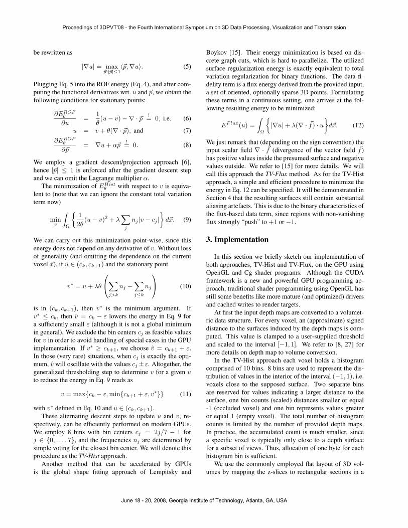
Further, we provide a visual comparison between the TV-Hist approach and the TV-Flux method (Eq. 12), which isthe continuous formulation of the global shape fitting en-ergy [15]. Figures 4(a) and (b) depict the final mesh ob-



Dataset Images Voxels Stereo Integration (CPU runtime [27]) Total Accuracy CompletenessTemple ring 47 200×300×160 8.8s 23.7s (3m27s) 32.5s 0.56mm 99.0%Temple 312 63s 83s — 2m23s 0.51mm 98.8%Dino ring 48 200×240×200 9.0s 26.4s (3m50s) 35.4s 0.51mm 99.1%Dino 363 70s 93s — 2m43s 0.55mm 98.7%

Table 1. The illustrated datasets and their characteristic information.

(a) “Temple”, front view (b) Back view (c) “Temple ring”, front view (d) Back view

Figure 2. Final meshes for the “Temple” and “Temple ring” datasets.

tained for the “Temple ring” data, and Figures 4(c) and(d) show more detailed views of the models generated us-ing TV-Flux and TV-Hist, respectively. The regularizationweight is set to λ = 0.3 in order to obtain visually simi-lar results. The overall geometry returned by the TV-Fluxapproach is comparable in quality with TV-Hist results, butcloseup views reveal the inherent binary nature of TV-Fluxsolutions.

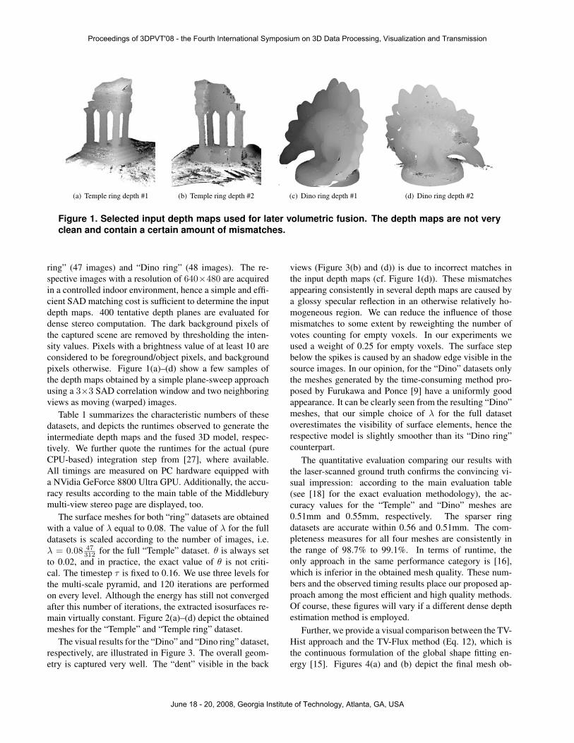
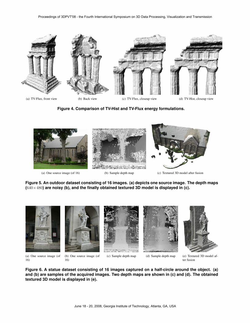
Finally, we provide results for outdoor image sequences.The first dataset consists of 16 views (see Figure 5(a)). Thedepth maps are computed by a local stereo approach usingnormalized cross correlation and a 5× 5 support window(Figure 5(b)). Range image fusion is performed using a320×120×200 voxel grid. The obtained 3D model aug-mented with surface texture derived from the input imagescan be seen in Figure 5(c). A statue dataset with sample in-put images, intermediate depth maps and the final 3D modelis displayed in Figure 6(a)–(e). The voxel grid resolution is144×288×200.

5. Conclusion and Future Work

In this work we present an efficient method for volumet-ric range image integration yielding high quality surface re-constructions from a given set of depth maps. The proposedprocedure is very suitable to be performed on highly par-

allel working stream processors. In particular, we reportruntime and accuracy evaluations for our GPU-acceleratedimplementation. We demonstrate that the achieved runtimeperformance is in the range of the currently fastest densemulti-view reconstruction method, while our approach re-turns very accurate 3D models at the same time.

Future work will address direct methods for multi-viewstereo reconstructions. The photoflux shape optimizationapproach [3] is a promising starting point for such investi-gations. Again, a continuous formulation of the surface reg-ularization energy will presumably lead to a simple and ef-ficient method for multi-view reconstruction. Additionally,further research is needed to extend the class of smoothnessterms that give rise to efficient and globally optimal algo-rithms.

References

[1] N. Amenta, S. Choi, and R. Kolluri. The power crust. In Pro-ceedings of 6th ACM Symposium on Solid Modeling, pages249–260, 2001.

[2] J.-D. Boissonnat and F. Cazals. Smooth surface reconstruc-tion via natural neighbour interpolation of distance func-tions. In Symposium on Computational Geometry, pages223–232, 2000.

[3] Y. Boykov and V. Lempitsky. From photohulls to photofluxoptimization. In British Machine Vision Conference(BMVC), pages 1149–1158, 2006.



(a) “Dino”, front view (b) Back view (c) “Dino ring”, front view (d) Back view

Figure 3. Final meshes for the “Dino” and “Dino ring” datasets.

[4] N. Campbell, G. Vogiatzis, C. Hernandez, and R. Cipolla.Automatic 3D object segmentation in multiple views usingvolumetric graph-cuts. In British Machine Vision Confer-ence, 2007.

[5] A. Chambolle. An algorithm for total variation minimiza-tion and applications. Journal of Mathematical Imaging andVision, 20(1–2):89–97, 2004.

[6] A. Chambolle. Total variation minimization and a class ofbinary MRF models. In Energy Minimization Methods inComputer Vision and Pattern Recognition, pages 136–152,2006.

[7] N. Cornelis and L. Van Gool. Real-time connectivity con-strained depth map computation using programmable graph-ics hardware. In Proc. CVPR, pages 1099–1104, 2005.

[8] B. Curless and M. Levoy. A volumetric method for build-ing complex models from range images. In Proceedings ofSIGGRAPH ’96, pages 303–312, 1996.

[9] Y. Furukawa and J. Ponce. Accurate, dense, and robustmulti-view stereopsis. In Proc. CVPR, 2007.

[10] A. Hilton, A. J. Stoddart, J. Illingworth, and T. Windeatt.Reliable surface reconstruction from multiple range images.In Proc. ECCV, pages 117–126, 1996.

[11] A. Hornung and L. Kobbelt. Hierarchical volumetric multi-view stereo reconstruction of manifold surfaces based ondual graph embedding. In Proc. CVPR, pages 503–510,2006.

[12] A. Hornung and L. Kobbelt. Robust reconstruction of water-tight 3D models from non-uniformly sampled point cloudswithout normal information. In Eurographics Symposium onGeometry Processing, pages 41–50, 2006.

[13] M. Kazhdan. Reconstruction of solid models from orientedpoint sets. In Symposium on Geometry Processing, pages73–82, 2005.

[14] M. Kazhdan, M. Bolitho, and H. Hoppe. Poisson surface re-construction. In Symposium on Geometry Processing, pages61–70, 2006.

[15] V. Lempitsky and Y. Boykov. Global optimization for shapefitting. In Proc. CVPR, 2007.

[16] P. Merrell, A. Akbarzadeh, L. Wang, P. Mordohai, J.-M.Frahm, R. Yang, D. Nister, and M. Pollefeys. Real-timevisibility-based fusion of depth maps. In Proc. ICCV, 2007.

[17] L. I. Rudin, S. Osher, and E. Fatemi. Nonlinear total vari-ation based noise removal algorithms. Physica D, 60:259–268, 1992.

[18] S. Seitz, B. Curless, J. Diebel, D. Scharstein, and R. Szeliski.A comparison and evaluation of multi-view stereo recon-struction algorithms. In Proc. CVPR, pages 519–526, 2006.

[19] S. Seitz and C. Dyer. Photorealistic scene reconstruction byvoxel coloring. IJCV, 35(2):151–173, 1999.

[20] C. Strecha, R. Fransens, and L. V. Gool. Combined depthand outlier estimation in multi-view stereo. In Proc. CVPR,pages 2394–2401, 2006.

[21] S. Tran and L. Davis. 3d surface reconstruction using graphcuts with surface constraints. In Proc. ECCV, pages 219–231, 2006.

[22] G. Turk and M. Levoy. Zippered polygon meshes from rangeimages. In Proceedings of SIGGRAPH ’94, pages 311–318,1994.

[23] G. Vogiatzis, P. Torr, and R. Cipolla. Multi-view stereovia volumetric graph-cuts. In Proc. CVPR, pages 391–398,2005.

[24] M. Wheeler, Y. Sato, and K. Ikeuchi. Consensus surfacesfor modeling 3d objects from multiple range images. InIEEE International Conference on Computer Vision (ICCV),pages 917 – 924, 1998.

[25] R. Yang and M. Pollefeys. Multi-resolution real-time stereoon commodity graphics hardware. In Proc. CVPR, pages211–217, 2003.

[26] A. Yezzi and S. Soatto. Stereoscopic segmentation. Int.Journal of Computer Vision, 53(1):31–43, 2003.

[27] C. Zach, T. Pock, and H. Bischof. A globally optimal al-gorithm for robust TV-L1 range image integration. In Proc.ICCV, 2007.

[28] C. Zach, M. Sormann, and K. Karner. High-performancemulti-view reconstruction. In Proc. 3DPVT, 2006.

[29] H.-K. Zhao, S. Osher, and R. Fedkiw. Fast surface recon-struction using the level set method. In IEEE Workshopon Variational and Level Set Methods in Computer Vision,pages 194–201, 2001.

[30] H.-K. Zhao, S. Osher, B. Merriman, and M. Kang. Implicitand nonparametric shape reconstruction from unorganizeddata using a variational level set method. Computer Visionand Image Understanding, 80(3):295–314, 2000.



(a) TV-Flux, front view (b) Back view (c) TV-Flux, closeup view (d) TV-Hist, closeup view

Figure 4. Comparison of TV-Hist and TV-Flux energy formulations.

(a) One source image (of 16) (b) Sample depth map (c) Textured 3D model after fusion

Figure 5. An outdoor dataset consisting of 16 images. (a) depicts one source image. The depth maps(640×480) are noisy (b), and the finally obtained textured 3D model is displayed in (c).

(a) One source image (of16)

(b) One source image (of16)

(c) Sample depth map (d) Sample depth map (e) Textured 3D model af-ter fusion

Figure 6. A statue dataset consisting of 16 images captured on a half-circle around the object. (a)and (b) are samples of the acquired images. Two depth maps are shown in (c) and (d). The obtainedtextured 3D model is displayed in (e).



fast and high quality fusion of depth maps...fast and high quality fusion of depth maps christopher...

Documents