Real-Time Visibility-Based Fusion of Depth Maps

Paul Merrell1, Amir Akbarzadeh2, Liang Wang2, Philippos Mordohai1, Jan-Michael Frahm1,Ruigang Yang2, David Nister2, and Marc Pollefeys1

1Department of Computer Science 2 Center for Visualization and Virtual EnvironmentsUniversity of North Carolina, Chapel Hill, USA University of Kentucky, Lexington, USA

Abstract

We present a viewpoint-based approach for the quick fu-sion of multiple stereo depth maps. Our method selectsdepth estimates for each pixel that minimize violations ofvisibility constraints and thus remove errors and inconsis-tencies from the depth maps to produce a consistent surface.We advocate a two-stage process in which the first stagegenerates potentially noisy, overlapping depth maps from aset of calibrated images and the second stage fuses thesedepth maps to obtain an integrated surface with higher ac-curacy, suppressed noise, and reduced redundancy. Weshow that by dividing the processing into two stages weare able to achieve a very high throughput because weare able to use a computationally cheap stereo algorithmand because this architecture is amenable to hardware-accelerated (GPU) implementations. A rigorous formula-tion based on the notion of stability of a depth estimate ispresented first. It aims to determine the validity of a depthestimate by rendering multiple depth maps into the refer-ence view as well as rendering the reference depth mapinto the other views in order to detect occlusions and free-space violations. We also present an approximate alterna-tive formulation that selects and validates only one hypoth-esis based on confidence. Both formulations enable us toperform video-based reconstruction at up to 25 frames persecond. We show results on the Multi-View Stereo Eval-uation benchmark datasets and several outdoors video se-quences. Extensive quantitative analysis is performed usingan accurately surveyed model of a real building as groundtruth.

1. Introduction

The problem of 3D reconstruction from video is a veryimportant topic in computer vision. It has received renewedattention recently due to applications such as Google Earthand Microsoft Virtual Earth which have been introducedfor delivering effective visualizations of large scale mod-els based on aerial and satellite imagery. This has sparked

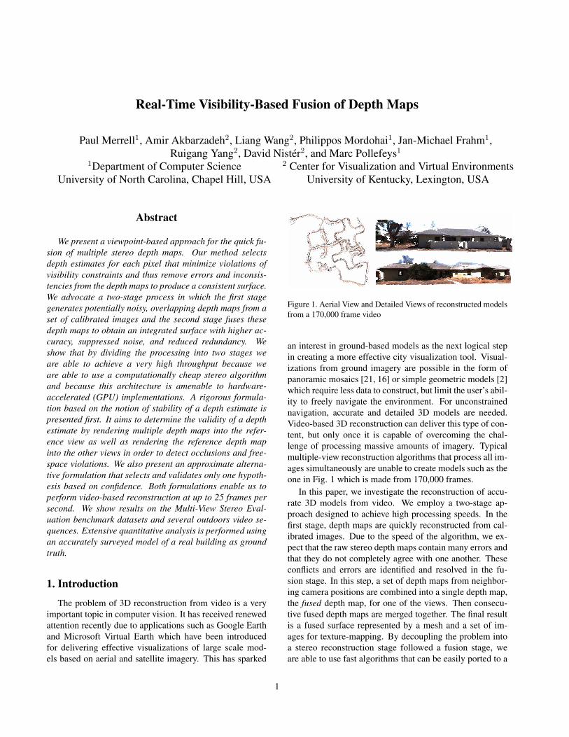
Figure 1. Aerial View and Detailed Views of reconstructed modelsfrom a 170,000 frame video

an interest in ground-based models as the next logical stepin creating a more effective city visualization tool. Visual-izations from ground imagery are possible in the form ofpanoramic mosaics [21, 16] or simple geometric models [2]which require less data to construct, but limit the user’s abil-ity to freely navigate the environment. For unconstrainednavigation, accurate and detailed 3D models are needed.Video-based 3D reconstruction can deliver this type of con-tent, but only once it is capable of overcoming the chal-lenge of processing massive amounts of imagery. Typicalmultiple-view reconstruction algorithms that process all im-ages simultaneously are unable to create models such as theone in Fig. 1 which is made from 170,000 frames.

In this paper, we investigate the reconstruction of accu-rate 3D models from video. We employ a two-stage ap-proach designed to achieve high processing speeds. In thefirst stage, depth maps are quickly reconstructed from cal-ibrated images. Due to the speed of the algorithm, we ex-pect that the raw stereo depth maps contain many errors andthat they do not completely agree with one another. Theseconflicts and errors are identified and resolved in the fu-sion stage. In this step, a set of depth maps from neighbor-ing camera positions are combined into a single depth map,the fused depth map, for one of the views. Then consecu-tive fused depth maps are merged together. The final resultis a fused surface represented by a mesh and a set of im-ages for texture-mapping. By decoupling the problem intoa stereo reconstruction stage followed a fusion stage, weare able to use fast algorithms that can be easily ported to a

1

programmable Graphics Processing Unit (GPU). Since it isimpossible to process thousands of images simultaneously,processing is performed in a sliding window.

Another benefit of the fusion step is that it producesa compact representation of the data since the number offused depth maps that are outputted is a small fraction ofthe original number of depth maps. Much of the infor-mation in the original depth maps is redundant since manynearby viewpoints observe the same surface. After fusion,the surface is constructed by detecting any overlap betweenconsecutive fused depth maps and merging the overlappingsurfaces. A compact representation is especially importantfor long video sequences since it allows the end-user to vi-sualize very large models.

2. Related WorkLarge scale reconstruction systems typically generate

partial reconstructions which are then merged. Conflictsand errors in these partial reconstructions are identified andresolved during the merging process. Surface fusion hasreceived considerable attention in the literature mostly fordata produced by range finders, where the noise level andthe fraction of outliers is typically lower than what is en-countered using passive sensors. Multiple-view reconstruc-tion methods based only on images have also been thor-oughly investigated [19], but many of them are limited tosingle objects and can not be applied to large scale scenesdue to computation and memory requirements.

Turk and Levoy [22] proposed a method for registeringand merging two triangular meshes. They remove any over-lapping parts of the meshes, connect the mesh boundariesand then update the positions of the vertices. Soucy andLaurendeau [20] introduced a similar algorithm which firstupdates the positions of the vertices and then connects themto form the triangular mesh. A different approach was pre-sented by Curless and Levoy [3] who employ a volumet-ric representation of the space and compute a cumulativeweighted distance function from the depth estimates. Thissigned distance function is an implicit representation of thesurface. A volumetric approach that explicitly takes into ac-count boundaries and holes was published by Hilton et al.[8]. Wheeler et al. [23] adapted the method of [3] to onlyconsider potential surfaces in voxels that are supported bysome consensus, instead of just one range image, to increaseits robustness to outliers. An online algorithm that uses astructured light sensor was introduced by Rusinkiewicz etal. [17]. It can merge partial reconstructions in the form ofpoint clouds in real-time by quantizing the space in voxelsand aggregating the information in each voxel. A slower,more accurate algorithm was also described.

Among the first approaches for passive data was thatof Fua [4] who adopted a particle based representation.The positions and orientations of the particles are initial-

ized from the depth estimates and modulated according toan image-based cost function and smoothness. Koch et al.[10] first establish binocular pixel correspondences and thenpropagate them to more images. When a match is consis-tent with a new camera, the camera is added to the chainthat supports the match. The position of the point is updatedusing the wider baseline, reducing the sensitivity to noise.Narayanan et al. [13] compute depth maps using multi-baseline stereo and merge them to produce viewpoint-basedvisible surface models. Holes due to occlusion are filled infrom nearby depth maps. Hernandez et al. [7] compute theprobability that a point in a volumetric grid is visible fromdepth maps and then segment the volume into foregroundand background using graph cuts.

Koch et al. [11] also presented a volumetric approachfor fusion. Given depth maps for all images, the depthestimates for all pixels are projected in the voxelized 3Dspace. Each depth estimate votes for a voxel probabilisti-cally and the surfaces are extracted by thresholding. Satoet al. [18] also advocated a volumetric method based onvoting. Each depth estimate votes not only for the mostlikely surface but also for the presence of free space be-tween the camera and the surface. Morency et al. [12] op-erate on a linked voxel space to rapidly produce triangula-tions. Information is fused in each voxel while connectivityinformation is maintained and updated in order to producethe final meshes. Goesele et al. [6] presented a two-stageapproach which merges depth maps produced by a simplealgorithm. Normalized cross-correlation is computed foreach depth estimate between the reference view and severaltarget views. The depth estimates are rejected if the cross-correlation is not large enough for at least two target views.The remaining depth estimates are used for surface recon-struction using the technique of [3].

3. Plane-Sweeping StereoIn the first of the two processing stages, depth maps

are computed from a set of images captured by a mov-ing camera with known pose, using plane-sweeping stereo[1, 5, 24]. Plane-sweeping was chosen primarily becauseit can be computed efficiently on the GPU, but since thetwo stages are designed to operate independently, any otherstereo matching algorithm could have been used instead.

The depth maps are computed using the plane-sweepingtechnique described in [5]. Each depth map is computedfor the central image in a set of typically 5 to 11 images.At each pixel, several depth hypotheses are tested in theform of planes. For each plane hypothesis, the depth fora pixel is computed by intersecting the ray emanating fromthe pixel with the hypothesized plane. All images are pro-jected onto the plane, via a set of homographies, and a costfor the hypothesized depth is calculated based on how wellthe images match on the plane. Here, we use absolute inten-

sity difference as the cost. The set of images is divided intwo halves, one preceding and one following the referenceimage. The sum of the absolute differences between eachhalf of the images and the reference view, projected ontothe plane, is calculated in square windows. The minimumof the two sums is the cost of the depth hypothesis [9]. Thisscheme is effective against occlusions, since in general thevisibility of a pixel does not change more than once duringan image sequence. The depth of each pixel is estimatedto be the depth d0 with the lowest cost. Each pixel is pro-cessed independently which allows non-planar surfaces tobe reconstructed.

The depth with the lowest cost may not be the true depthdue to noise, occlusion, lack of texture, surfaces that are notaligned with the plane direction, and many other factors.Parts of the image with little texture are especially difficultto accurately reconstruct using stereo. A measurement ofthe confidence of each depth estimate is important. To es-timate the confidence, we use the following heuristic. Weassume the cost is perturbed by Gaussian noise. Let c(x, d)be the matching cost for depth d at pixel x. We wish to es-timate the likelihood that the true depth, do, does not havethe lowest cost after the cost is perturbed. This likelihood isproportional to: e−(c(x,d)−c(x,d0))2/σ2

for some σ that de-pends on the strength of the noise. The confidence C(x) isdefined as the inverse of the sum of these probabilities forall possible depths:

C(x) =

∑d 6=d0

e−(c(x,d)−c(x,d0))2/σ2

−1

(1)

This equation produces a high confidence when the costhas a single sharp minimum. The confidence is low whenthe cost has a shallow minimum or several low minima.

4. Visibility-Based Depth Map FusionDue to the speed of the stereo algorithm, the raw stereo

depth maps contain errors and do not completely agree witheach other. These conflicts and errors are identified and re-solved in the fusion stage. In this step, a set of depth mapsfrom neighboring camera positions are combined into a sin-gle fused depth map for one of the views. From the fuseddepth maps we show how to construct a triangulated surfacein Sec. 4.3.

The input to the fusion step is a set of N depth mapsdenoted by D1(x), D2(x), . . . , DN (x) which record theestimated depth of each pixel of the N images. Eachdepth map has an associated confidence map labeledC1(x), C2(x), . . . , CN (x) computed according to (1). Oneof the viewpoints, typically the central one, is selected asthe reference viewpoint. We seek a depth estimate for eachpixel of the reference view. The current estimate of the

3D point seen at pixel x of the reference view is calledF (x). Ri(X) is the distance between the center of projec-tion of viewpoint i and the 3D point X. We define the termf(x) ≡ Rref (F (x)) which is the distance of the currentdepth estimate F (x) for the reference camera.

The first step of fusion is to render each depth map intothe reference view. When multiple depth values project ontothe same pixel, the nearest depth is kept. Let Dref

i be thedepth mapDi rendered into the reference view and Crefi bethe confidence map rendered in the reference view. Given a3D point X, we need a notation to describe the value of thedepth map Di at the location where X projects into viewi. Let Pi(X) be the image coordinates of the 3D point Xprojected into view i. To simplify the notation, we definethe term Di(X) ≡ Di(Pi(X)). Di(X) is likely to be dif-ferent fromRi(X) which is the distance between X and thecamera center.

Our approach considers three types of visibility relation-ships between hypothesized depths in the reference viewand computed depths in the other views. These relationsare illustrated in Fig. 2(a). The point A′ observed in view iis behind the point A observed in the reference view. Thereis a conflict between the measurement and the hypothesizeddepth since view i would not be able to observe A′ if theretruly was a surface at A. We say that A violates the freespace of A′. This occurs when Ri(A) < Di(A).

In Fig. 2(a), B′ is in agreement with B since they are inthe same location. In practice, we define points B and B′

as being in agreement when |Rref (B)−Rref (B′)|Rref (B) < ε.

The point C ′ observed in view i is in front of the pointC observed in the reference view. There is a conflict be-tween these two measurements since it would be impossibleto observe C if there truly was a surface at C ′. We say thatC ′ occludes C. This occurs when Dref

i (C′) < f(C) =Dref (C).

Note that operations for a pixel are not performed on asingle ray, but on rays from all cameras. Occlusions aredefined on the rays of the reference view, but free spaceviolations are defined on the rays of the other depth maps.The reverse depth relations (such as A behind A′ or C infront of C ′) do not represent visibility conflicts.

The raw stereo depth maps give different estimates of thedepth at a given pixel in the reference view. We first presenta method that tests each of these estimates and selects themost likely candidate by exhaustively considering all occlu-sions and free-space constraints. We then present an alter-native approach that selects a likely candidate upfront basedon the confidence and then verifies that this estimate agreeswith most of the remaining data. The type of computationsrequired in both approaches are quite similar. Most of thecomputation time is spent rendering a depth map seen inone viewpoint into another viewpoint. These computationscan be performed efficiently on the GPU.

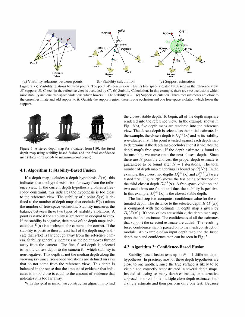
(a) Visibility relations between points (b) Stability calculation (c) Support estimationFigure 2. (a) Visibility relations between points. The point A′ seen in view i has its free space violated by A seen in the reference view.B′ supports B. C seen in the reference view is occluded by C′. (b) Stability Calculation. In this example, there are two occlusions whichraise stability and one free-space violations which lowers it. The stability is +1. (c) Support calculation. Three measurements are close tothe current estimate and add support to it. Outside the support region, there is one occlusion and one free-space violation which lower thesupport.

Figure 3. A stereo depth map for a dataset from [19], the fuseddepth map using stability-based fusion and the final confidencemap (black corresponds to maximum confidence).

4.1. Algorithm 1: Stability-Based Fusion

If a depth map occludes a depth hypothesis F (x), thisindicates that the hypothesis is too far away from the refer-ence view. If the current depth hypothesis violates a free-space constraint, this indicates the hypothesis is too closeto the reference view. The stability of a point S(x) is de-fined as the number of depth maps that occlude F (x) minusthe number of free-space violations. Stability measures thebalance between these two types of visibility violations. Apoint is stable if the stability is greater than or equal to zero.If the stability is negative, then most of the depth maps indi-cate that F (x) is too close to the camera to be correct. If thestability is positive then at least half of the depth maps indi-cate that F (x) is far enough away from the reference cam-era. Stability generally increases as the point moves furtheraway from the camera. The final fused depth is selectedto be the closest depth to the camera for which stability isnon-negative. This depth is not the median depth along theviewing ray since free-space violations are defined on raysthat do not come from the reference view. This depth isbalanced in the sense that the amount of evidence that indi-cates it is too close is equal to the amount of evidence thatindicates it is too far away.

With this goal in mind, we construct an algorithm to find

the closest stable depth. To begin, all of the depth maps arerendered into the reference view. In the example shown inFig. 2(b), five depth maps are rendered into the referenceview. The closest depth is selected as the initial estimate. Inthe example, the closest depth isDref

1 (x) and so its stabilityis evaluated first. The point is tested against each depth mapto determine if the depth map occludes it or if it violates thedepth map’s free space. If the depth estimate is found tobe unstable, we move onto the next closest depth. Sincethere are N possible choices, the proper depth estimate isguaranteed to be found after N − 1 iterations. The totalnumber of depth map renderings is bound byO(N2). In theexample, the closest two depthsDref

1 (x) andDref3 (x) were

tested first. Figure 2(b) shows the test being performed onthe third closest depth Dref

2 (x). A free-space violation andtwo occlusions are found and thus the stability is positive.In this example, Dref

2 (x) is the closest stable depth.The final step is to compute a confidence value for the es-

timated depth. The distance to the selected depth Ri(F (x))is compared with the estimate in depth map i given byDi(F (x)). If these values are within ε, the depth map sup-ports the final estimate. The confidences of all the estimatesthat support the selected estimate are added. The resultingfused confidence map is passed on to the mesh constructionmodule. An example of an input depth map and the fuseddepth map and confidence map can be seen in Fig. 3.

4.2. Algorithm 2: Confidence-Based Fusion

Stability-based fusion tests up to N − 1 different depthhypotheses. In practice, most of these depth hypotheses areclose to one another, since the true surface is likely to bevisible and correctly reconstructed in several depth maps.Instead of testing so many depth estimates, an alternativeapproach is to combine multiple close depth estimates intoa single estimate and then perform only one test. Because

there is only one hypothesis to test, there are only O(N)renderings to compute. This approach is typically fasterthan stability-based fusion which tests N − 1 hypothesesand computesO(N2) renderings, but the early commitmentmay introduce additional errors.

Combining Consistent Estimates Confidence-based fu-sion also begins by rendering all the depth maps into thereference view. The depth estimate with the highest confi-dence is selected as the initial estimate for each pixel. Ateach pixel x, we keep track of two quantities which are up-dated iteratively: the current depth estimate and its level ofsupport. Let f0(x) and C0(x) be the initial depth estimateand its confidence value. fk(x) and Ck(x) are the depthestimate and its support at iteration k, while F (x) is thecorresponding 3D point.

If another depth mapDrefi (x) produces a depth estimate

within ε of the initial depth estimate f0(x), it is very likelythat the two viewpoints have both correctly reconstructedthe same surface. In the example of Fig. 2(c), the esti-mates D3(F (x)) and D5(F (x)) are close to the initial es-timate. These close observations are averaged into a singleestimate. Each observation is weighted by its confidenceaccording to the following equations:

fk+1(x) =fk(x)Ck(x) +Dref

i (x)Ci(x)Ck(x) + Ci(x)

(2)

Ck+1(x) = Ck(x) + Ci(x) (3)

The result is a combined depth estimate fk(x) at eachpixel of the reference image and a support level Ck(x) mea-suring how well the depth maps agree with the depth esti-mate. The next step is to find how many of the depth mapscontradict fk(x) in order to verify its correctness.

Conflict Detection The total amount of support for eachdepth estimate must be above the threshold Cthres or elseit is discarded as an outlier and is not processed any fur-ther. The remaining points are checked using visibility con-straints. Figure 2(c) shows that D1(F (x)) and D3(F (x))occlude F (x). However,D3(F (x)) is close enough (withinε) to F (x) to be within its support region and so this occlu-sion does not count against the current estimate. D1(F (x))is occluding F (x) outside the support region and thus con-tradicts the current estimate. When such an occlusion takesplace the support of the current estimate is decreased by:

Ck+1(x) = Ck(x)− Crefi (x) (4)

When a free-space violation occurs outside the supportregion, as occurs with the depth D4(F (x)) in Fig. 2(c), theconfidence of the conflicting depth estimate is subtractedfrom the support according to:

Ck+1(x) = Ck(x)− Ci(Pi(F (x))) (5)

We have now added the confidence of all the depth mapsthat support the current depth estimate and subtracted theconfidence of all those that contradict it. If the support ispositive, the majority of the evidence supports the depth es-timate and it is kept. If the support is negative, the depthestimate is discarded as an outlier. The fused depth map atthis stage contains estimates with high confidence and holeswhere the estimates have been rejected.

Hole filling After discarding the outliers, there are manyholes in the fused depth map. In practice, the depth mapsof most real-world scenes are piecewise smooth and we as-sume that any small missing parts of the depth map are mostlikely to have a depth close to their neighbors. To fill in thegaps, we find all inliers within a w×w window centered atthe pixel we wish to estimate. If there are enough inliers tomake a good estimate, we assign the median of the inliersas the depth of the pixel. If there are only a few neighbor-ing inliers, the depth map is left blank. Essentially, this isa median filter that ignores the outliers. In the final step, amedian filter with a smaller window ws is used to smoothout the inliers.

4.3. Surface Reconstruction

We have presented two algorithms for generating fuseddepth maps. Consecutive fused depth maps partially over-lap one another. It is likely that these overlapping surfaceswill not be aligned perfectly. The desired output of our sys-tem is a smooth and consistent model of the scene. To thisend, consistency between consecutive fused depth maps isenforced in the final model. Each fused depth map is com-pared with the previous fused depth map as it is being gen-erated. If a new estimate violates the free space of the previ-ous fused depth maps, the new estimate is rejected. If a newdepth estimate is within ε of the previous fused depth map,the two estimates are merged into one vertex which is gen-erated only once in the output. Thus redundancy is removedalong with any gaps in the model where two representationsof the same surface are not connected. More than one previ-ous fused depth map should be kept in memory to properlyhandle surfaces that disappear and become visible again. Inmost cases, two previous fused depth maps are sufficient.

After duplicate surface representations have beenmerged, a mesh is constructed taking into account the cor-responding confidence map to suppress any remaining out-liers. By using the image plane as a reference both for ge-ometry and for appearance, we can construct a triangularmesh very quickly. We employ a multi-resolution quad-tree algorithm in order to minimize the number of triangleswhile maintaining geometric accuracy as in [14]. We use

a top-down approach rather than a bottom-up approach tolower the number of triangles that need to be processed.Starting from a coarse resolution, we form triangles and testif they correspond to nonplanar parts of the depth map, ifthey bridge depth discontinuities or if points with low con-fidence (below Cthres) are included within them. If any ofthese events occur, the quad, which is formed out of two ad-jacent triangles, is subdivided. The process is repeated onthe subdivided quads up to the finest resolution.

We use the following simple planarity test proposed in[15] for each vertex of each triangle:∣∣∣∣z−1 − z0

z−1− z0 − z1

z1

∣∣∣∣ < t. (6)

Where z0 is the z-coordinate, in the camera coordinate sys-tem, of the vertex being tested and t is a threshold. z−1

and z1 are the z-coordinates of the two neighboring verticesof the current vertex on an image row. (The distance be-tween the corresponding pixels of two neighboring verticesis equal to the size of the quad’s edges.) The same test isrepeated along an image column. If either the vertical orthe horizontal tests fails for any of the vertices of the trian-gle, the triangle is not part of a planar surface and so thequad is subdivided. For these tests, we have found that 3Dcoordinates are more effective than disparity values. Sincewe do not require a manifold mesh and are interested in fastprocessing speeds, we do not maintain a restricted quad-tree[14].

5. Results

Our methods were tested on videos of urban environ-ments and on the Multi-View Stereo Evaluation dataset(http://vision.middlebury.edu/mview/) [19]. On the ur-ban datasets, the plane-sweeping stereo algorithm used 48planes and matched 7 images to obtain each stereo depthmap. Every 17 frames, 17 stereo depth maps were usedto produce a fused depth map. Using these settings andstability-based fusion a processing rate of 23 frames persecond can be achieved on a high-end personal computerwith an NVidia GeForce 8800 GPU. If confidence-basedfusion is used instead, processing speed reaches 25 framesper second. On the Multi-View dataset, the plane-sweepingstep used 94 planes and matched five images. Every fiveframes, 15 stereo depth maps were fused together. Onboth datasets, the following parameters were used: ε =0.05, σ = 120, w = 8 pixels, ws = 4 pixels, and Cthres =5. The image sizes are 512 × 384 for the urban videos and640× 480 for the Multi-View dataset.

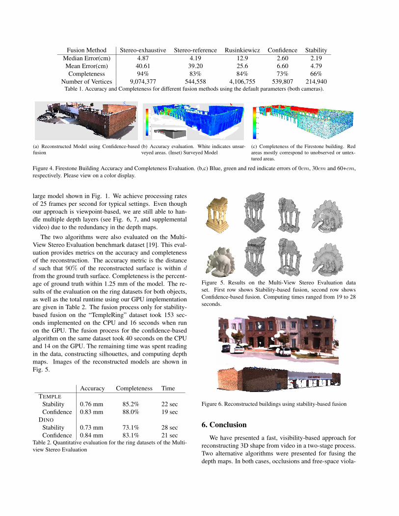
To evaluate the ability of our method to reconstruct urbanenvironments, a 3,000 frame video of the exterior of a Fire-stone store was captured with two cameras to obtain a morecomplete reconstruction. One of the cameras was pointed

horizontally and the other was tilted up 30o. The videosfrom each camera were processed separately. The Firestonebuilding was surveyed to an accuracy of 6 mm and the re-constructed model (Fig. 4(a)) was directly compared withthe surveyed model (Fig. 4(b) inset). There are several ob-jects such as parked cars that are visible in the video, butwere not surveyed. The ground which slopes away fromthe building also was not surveyed. Objects included inthe video that were not surveyed were manually removedfrom the evaluation. To measure the accuracy of each re-constructed vertex, the distance from the vertex to the near-est triangle of the ground truth model is calculated. Theerror measurements for each part of a reconstructed modelare displayed in Fig. 4(b). We also evaluated the complete-ness of the reconstruction which measures how much ofthe building was reconstructed and is defined similar to thecompleteness measurement in [19]. Sample points are cho-sen at random on the surface of the ground truth model witha density of 50 sample points per square meter of surfacearea. The distance from each sample point to the nearest re-constructed point is measured. A visualization of these dis-tances is shown for one of the reconstructions in Fig. 4(c).

We performed a quantitative evaluation between rawstereo depth maps and the results of the fusion algorithms.For the results labeled as stereo-reference, we evaluate theraw depth maps from each of the fusion reference views.For the results labeled stereo-exhaustive, we evaluated thedepth maps from all images as the representation of thescene. We also implemented the real-time algorithm ofRusinkiewicz et al. [17] using a grid of 5cm voxels. Thisalgorithm produces a point cloud from which surface re-construction is not trivial. Table 1 contains the median andmean error values for each method as well as the complete-ness achieved on the Firestone building. Volumetric meth-ods that handle outliers such as [23] could be applied in oursettings, but they would not be real-time.

The results show that the raw stereo depth mapsare highly inaccurate and contain many large outliers.Confidence-based and stability-based fusion improve theaccuracy of the reconstruction, but lose some completeness,since some of the points removed as outliers might havebeen near the surface. Depth estimates created in the hole-filling stage of confidence-based fusion are not guaranteedto satisfy visibility constraints, but are typically reasonableresulting in increased completeness at the expense of someaccuracy as shown in the results. The real-time techniqueof Rusinkiewicz et al. [17] does not improve accuracy anddoes not reduce the number of points in the model effec-tively without a significant loss of resolution.

Our methods were also used on several videos of urbanenvironments using the same camera configuration and set-tings. The reconstructed models are shown in Fig. 6 and 7.A very long 170,000 frame video was used to reconstruct a

Fusion Method Stereo-exhaustive Stereo-reference Rusinkiewicz Confidence StabilityMedian Error(cm) 4.87 4.19 12.9 2.60 2.19Mean Error(cm) 40.61 39.20 25.6 6.60 4.79Completeness 94% 83% 84% 73% 66%

Number of Vertices 9,074,377 544,558 4,106,755 539,807 214,940Table 1. Accuracy and Completeness for different fusion methods using the default parameters (both cameras).

(a) Reconstructed Model using Confidence-basedfusion

(b) Accuracy evaluation. White indicates unsur-veyed areas. (Inset) Surveyed Model

(c) Completeness of the Firestone building. Redareas mostly correspond to unobserved or untex-tured areas.

Figure 4. Firestone Building Accuracy and Completeness Evaluation. (b,c) Blue, green and red indicate errors of 0cm, 30cm and 60+cm,respectively. Please view on a color display.

large model shown in Fig. 1. We achieve processing ratesof 25 frames per second for typical settings. Even thoughour approach is viewpoint-based, we are still able to han-dle multiple depth layers (see Fig. 6, 7, and supplementalvideo) due to the redundancy in the depth maps.

The two algorithms were also evaluated on the Multi-View Stereo Evaluation benchmark dataset [19]. This eval-uation provides metrics on the accuracy and completenessof the reconstruction. The accuracy metric is the distanced such that 90% of the reconstructed surface is within dfrom the ground truth surface. Completeness is the percent-age of ground truth within 1.25 mm of the model. The re-sults of the evaluation on the ring datasets for both objects,as well as the total runtime using our GPU implementationare given in Table 2. The fusion process only for stability-based fusion on the “TempleRing” dataset took 153 sec-onds implemented on the CPU and 16 seconds when runon the GPU. The fusion process for the confidence-basedalgorithm on the same dataset took 40 seconds on the CPUand 14 on the GPU. The remaining time was spent readingin the data, constructing silhouettes, and computing depthmaps. Images of the reconstructed models are shown inFig. 5.

Accuracy Completeness TimeTEMPLE

Stability 0.76 mm 85.2% 22 secConfidence 0.83 mm 88.0% 19 sec

DINOStability 0.73 mm 73.1% 28 secConfidence 0.84 mm 83.1% 21 sec

Table 2. Quantitative evaluation for the ring datasets of the Multi-view Stereo Evaluation

Figure 5. Results on the Multi-View Stereo Evaluation dataset. First row shows Stability-based fusion, second row showsConfidence-based fusion. Computing times ranged from 19 to 28seconds.

Figure 6. Reconstructed buildings using stability-based fusion

6. ConclusionWe have presented a fast, visibility-based approach for

reconstructing 3D shape from video in a two-stage process.Two alternative algorithms were presented for fusing thedepth maps. In both cases, occlusions and free-space viola-

Figure 7. Reconstructed buildings using confidence-based fusion

tions are used to guide the search for a plausible depth foreach pixel. Stability-based fusion is more robust and pro-duces slightly more accurate results. Since its complexityscales quadratically with the number of input depth maps, itbecomes significantly slower than confidence-based fusionas the number of depth maps increases. Confidence-basedfusion is a greedy algorithm since it makes an initial com-mitment to the most likely candidate. Its linear complexityallows for real-time performance on larger input sets.

Our methods are suitable for large scale reconstructionsbecause they can process large amounts of data in pipelinemode at rates near real time. The accuracy of the recon-struction was evaluated using a surveyed model of a realbuilding and was found to be accurate within a few centime-ters. We also participated in the Multi-View Stereo Evalu-ation obtaining satisfactory results with at least an order ofmagnitude faster processing than the state of the art. Our fu-ture work will focus on improving the visual quality of themodels by detecting features such as planar surfaces andstraight lines and ensuring they are represented as such.

Acknowledgments: Supported by the DTO under the VACEprogram and by DARPA under the UrbanScape project. Approvedfor Public Release, Distribution Unlimited.

Project Website: http://cs.unc.edu/Research/urbanscape/

References[1] R. Collins. A space-sweep approach to true multi-image

matching. In CVPR, pages 358–363, 1996.[2] N. Cornelis, K. Cornelis, and L. Van Gool. Fast compact city

modeling for navigation pre-visualization. In CVPR, 2006.[3] B. Curless and M. Levoy. A volumetric method for building

complex models from range images. SIGGRAPH, 30:303–312, 1996.

[4] P. Fua. From multiple stereo views to multiple 3-d surfaces.IJCV, 24(1):19–35, 1997.

[5] D. Gallup, J.-M. Frahm, P. Mordohai, Q. Yang, and M. Polle-feys. Real-time plane-sweeping stereo with multiple sweep-ing directions. In CVPR, 2007.

[6] M. Goesele, B. Curless, and S. M. Seitz. Multi-view stereorevisited. In CVPR, pages 2402–2409, 2006.

[7] C. Hernandez, G. Vogiatzis, and R. Cipolla. Probabilisticvisibility for multi-view stereo. In CVPR, 2007.

[8] A. Hilton, A. Stoddart, J. Illingworth, and T. Windeatt. Re-liable surface reconstruction from multiple range images. InCVPR, pages 117–126, 1996.

[9] S. Kang, R. Szeliski, and J. Chai. Handling occlusions indense multi-view stereo. In CVPR, pages 103–110, 2001.

[10] R. Koch, M. Pollefeys, and L. Van Gool. Multi viewpointstereo from uncalibrated video sequences. In ECCV, vol-ume I, pages 55–71, 1998.

[11] R. Koch, M. Pollefeys, and L. Van Gool. Robust calibrationand 3d geometric modeling from large collections of uncali-brated images. In DAGM, pages 413–420, 1999.

[12] L. Morency, A. Rahimi, and T. Darrell. Fast 3d model acqui-sition from stereo images. In 3DPVT, pages 172–176, 2002.

[13] P. Narayanan, P. Rander, and T. Kanade. Constructing virtualworlds using dense stereo. In ICCV, pages 3–10, 1998.

[14] R. Pajarola. Overview of quadtree-based terrain triangulationand visualization. Technical report, 2002.

[15] R. Pajarola, Y. Meng, and M. Sainz. Fast depth-image mesh-ing and warping. Technical report, 2002.

[16] A. Roman, G. Garg, and M. Levoy. Interactive design ofmulti-perspective images for visualizing urban landscapes.In IEEE Visualization, pages 537–544, 2004.

[17] S. Rusinkiewicz, O. Hall-Holt, and M. Levoy. Real-time 3dmodel acquisition. SIGGRAPH, 21(3):438–446, 2002.

[18] T. Sato, M. Kanbara, N. Yokoya, and H. Takemura. Dense3-d reconstruction of an outdoor scene by hundreds-baselinestereo using a hand-held video camera. IJCV, 47(1-3):119–129, 2002.

[19] S. M. Seitz, B. Curless, J. Diebel, D. Scharstein, andR. Szeliski. A comparison and evaluation of multi-viewstereo reconstruction algorithms. In CVPR, pages 519–528,2006.

[20] M. Soucy and D. Laurendeau. A general surface approach tothe integration of a set of range views. PAMI, 17(4):344–358,1995.

[21] S. Teller, M. Antone, Z. Bodnar, M. Bosse, S. Coorg,M. Jethwa, and N. Master. Calibrated, registered images ofan extended urban area. IJCV, 53(1):93–107, June 2003.

[22] G. Turk and M. Levoy. Zippered polygon meshes from rangeimages. In SIGGRAPH, pages 311–318, 1994.

[23] M. Wheeler, Y. Sato, and K. Ikeuchi. Consensus surfaces formodeling 3d objects from multiple range images. In ICCV,pages 917–924, 1998.

[24] R. Yang and M. Pollefeys. A versatile stereo implementa-tion on commodity graphics hardware. Journal of Real-TimeImaging, 11(1):7–18, 2005.