Fast Failure Recovery in Distributed Graph ProcessingSystems

Yanyan Shen§, Gang Chen†, H. V. Jagadish‡, Wei Lu¶∗, Beng Chin Ooi§, Bogdan Marius Tudor§

§National University of Singapore, †Zhejiang University, ‡University of Michigan, ¶Renmin University§{shenyanyan,ooibc,bogdan}@comp.nus.edu.sg, †cg@cs.zju.edu.cn, ‡jag@umich.edu, ¶luwei@ruc.edu.cn

ABSTRACTDistributed graph processing systems increasingly require manycompute nodes to cope with the requirements imposed by contem-porary graph-based Big Data applications. However, increasingthe number of compute nodes increases the chance of node fail-ures. Therefore, provisioning an efficient failure recovery strategyis critical for distributed graph processing systems. This paper pro-poses a novel recovery mechanism for distributed graph processingsystems that parallelizes the recovery process. The key idea is topartition the part of the graph that is lost during a failure amonga subset of the remaining nodes. To do so, we augment the exist-ing checkpoint-based and log-based recovery schemes with a par-titioning mechanism that is sensitive to the total computation andcommunication cost of the recovery process. Our implementationon top of the widely used Giraph system outperforms checkpoint-based recovery by up to 30x on a cluster of 40 compute nodes.

1. INTRODUCTIONGraphs capture complex relationships and data dependencies,

and are important to Big Data applications such as social networkanalysis, spatio-temporal analysis and navigation, and consumeranalytics. MapReduce was proposed as a programming model forBig Data about a decade ago, and since then, many MapReduce-based distributed systems have been designed for Big Data appli-cations such as large-scale data analytics [16]. However, in recentyears, MapReduce has been shown to be ineffective for handlinggraph data, and several new systems such as Pregel [20], Giraph[1], GraphLab [10, 18], and Trinity [24] have been recently pro-posed for scalable distributed graph processing.

With the explosion in graph size and increasing demand of com-plex analytics, graph processing systems have to continuously scaleout by increasing the number of compute nodes, in order to han-dle the load. But scaling the number of nodes has two effects onthe failure resilience of a system. First, increasing the number ofnodes will inevitably lead to an increase in the number of failednodes. Second, after a failure, the progress of the entire system is

∗This work is done at National University of Singapore.

Permission to make digital or hard copies of all or part of this work forpersonal or classroom use is granted without fee provided that copies arenot made or distributed for profit or commercial advantage and that copiesbear this notice and the full citation on the first page. To copy otherwise, torepublish, to post on servers or to redistribute to lists, requires prior specificpermission and/or a fee. Articles from this volume were invited to presenttheir results at The 41st International Conference on Very Large Data Bases,August 31st - September 4th 2015, Kohala Coast, Hawai’i.Proceedings of the VLDB Endowment, Vol. 8, No. 4Copyright 2014 VLDB Endowment 2150-8097/14/12.

halted until the failure is recovered. Thus, a potentially large num-ber of nodes will become idle just because a small set of nodes havefailed. In order to scale out the performance continuously when thenumber of nodes increases, it is becoming crucial to provision thegraph processing systems with the ability to handle the failures ef-fectively.

The design of failure recovery mechanisms in distributed sys-tems is a nontrivial task, as they have to cope with several adversar-ial conditions. Node failures may occur at any time, either duringnormal job execution, or during recovery period. The design of arecovery algorithm must be able to handle both kinds of failures.Furthermore, the recovery algorithm must be very efficient becausethe overhead of recovery can degrade system performance signifi-cantly. To a certain extent, due to the long recovery time, failuresmay occur repeatedly before the system recovers from an initialfailure. If so, the system will go into an endless recovery loop with-out any progress in execution. Finally, the system must cope withthe failures while maintaining the recovery mechanism transparentto user applications. This implies that the recovery algorithm canonly rely on the computation model of the system, rather than anycomputation logic applied for specific applications.

The usual recovery method adopted in current distributed graphprocessing systems is checkpoint-based [17, 20, 26]. It requireseach compute node to periodically and synchronously write the sta-tus of its own subgraph to a stable storage such as the distributed filesystem as a checkpoint. Upon any failure, checkpoint-based recov-ery employs an unused healthy compute node to replace each failednode and requires all the compute nodes to load the status of sub-graphs from the most recent checkpoint and then synchronously re-execute all the missing workloads. A failure is recovered when allthe nodes finish the computations that have been completed beforethe failure occurs. Note that the recomputation will be replayedagain whenever a further failure occurs during recovery.

Although checkpoint-based recovery is able to handle any nodefailures, it potentially suffers from high recovery latency. The rea-son is two-fold. First, checkpoint-based recovery re-executes themissing workloads over the whole graph, residing in both failedand healthy compute nodes, based on the most recent checkpoint.This could incur high computation cost as well as high commu-nication cost, including loading the whole checkpoint, performingrecomputation and passing the messages among all compute nodesduring the recovery. Second, when a further failure occurs duringthe recovery, the lost computation caused by the previous failuremay have been partially recovered. However, checkpoint-based re-covery will forget about all of this partially completed workload,rollback every compute node to the latest checkpoint and replaythe computation since then. This eliminates the possibility of per-forming the recovery progressively.

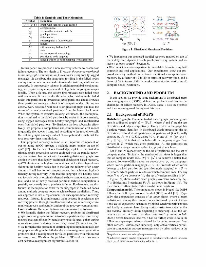
Table 1: Symbols and Their MeaningsSymbol DefinitionG = (V, E) graph with vertices V and edges E

N compute nodeVN vertices that reside in node NP graph partitionsNf failed nodessf superstep that a failure occursF failureF i i-th cascading failure for FS stateϕ vertex to partition mappingφp partition to node mappingφr failed partition to node mapping (reassignment)

In this paper, we propose a new recovery scheme to enable fastfailure recovery. The key idea is to 1) restrict the recovery workloadto the subgraphs residing in the failed nodes using locally loggedmessages; 2) distribute the subgraphs residing in the failed nodesamong a subset of compute nodes to redo the lost computation con-currently. In our recovery scheme, in addition to global checkpoint-ing, we require every compute node to log their outgoing messageslocally. Upon a failure, the system first replaces each failed nodewith a new one. It then divides the subgraphs residing in the failednodes into partitions, referred to as failed partitions, and distributesthese partitions among a subset S of compute nodes. During re-covery, every node in S will hold its original subgraph and load thestatus of its newly received partitions from the latest checkpoint.When the system re-executes missing workloads, the recomputa-tion is confined to the failed partitions by nodes in S concurrently,using logged messages from healthy subgraphs and recalculatedones from failed partitions. To distribute the lost subgraphs effec-tively, we propose a computation and communication cost modelto quantify the recovery time, and according to the model, we splitthe lost subgraphs among a subset of compute nodes such that thetotal recovery time is minimized.

Our proposed recovery scheme is an important component ofour on-going epiCG project: a scalable graph engine on top ofepiC [12]. To the best of our knowledge, epiCG is the first dis-tributed graph processing system equipped with the parallel recov-ery mechanism. In contract with the existing distributed graph pro-cessing systems that deploy traditional checkpoint-based recovery,epiCG eliminates the high recomputation cost for the subgraphs re-siding in the healthy nodes due to the fact that failures often occuramong a small fraction of compute nodes, thus achieving high ef-ficiency during recovery. Note that the subgraph in a healthy nodecan include both its original subgraph (whose computation is neverlost) and a set of newly received partitions (whose computation ispartially recovered) due to previous failures. Furthermore, we dis-tribute the recomputation tasks for the subgraphs in the failed nodesamong multiple compute nodes to achieve better parallelism. Thus,our approach is not a replacement for checkpoint-based recoverymethods. Instead, it complements them because it accelerates therecovery process through simultaneous reduction of recovery com-munication costs and parallelization of the recovery computations.Contributions. Our contributions are summarized as follows.• We formally define the failure recovery problem in distributedgraph processing systems and introduce a partition-based recoverymethod that can efficiently handle any node failures, either duringnormal execution or during the recovery period (Section 2 and 3).•We formalize the problem of distributing recomputation tasks forsubgraphs residing in the failed nodes as a reassignment generationproblem: find a reassignment for failed partitions with minimizedrecovery time. We show the problem is NP-hard and propose acost-sensitive reassignment algorithm (Section 4).

BA G

H

J

C

FE

D

I

(a) G(V, E)

BA

C D

FE

G H

JI

B

C

H

I D EB F

A B

C D

FE

G H

JI

Vertex Subgraph

G

(b) P

Figure 1: Distributed Graph and Partitions

• We implement our proposed parallel recovery method on top ofthe widely used Apache Giraph graph processing system, and re-lease it as open source1 (Section 5).•We conduct extensive experiments on real-life datasets using bothsynthetic and real applications. Our experiments show our pro-posed recovery method outperforms traditional checkpoint-basedrecovery by a factor of 12 to 30 in terms of recovery time, and afactor of 38 in terms of the network communication cost using 40compute nodes (Section 6).

2. BACKGROUND AND PROBLEMIn this section, we provide some background of distributed graph

processing systems (DGPS), define our problem and discuss thechallenges of failure recovery in DGPS. Table 1 lists the symbolsand their meaning used throughout this paper.

2.1 Background of DGPSDistributed graph. The input to distributed graph processing sys-tems is a directed graph2 G = (V, E), where V and E are the setsof vertices and edges, respectively. Every vertex in the graph hasa unique vertex identifier. In distributed graph processing, the setof vertices is divided into partitions. A partition of G is formallydenoted by Pi = (Vi, Ei), where Vi ⊆ V and Ei = {〈vi, vj〉 ∈E|vi ∈ Vi}. Note that Ei includes all the outgoing edges fromvertices in Vi, which may cross partitions. All the partitions aredistributed among compute nodes, i.e., physical machines.

Let P and N respectively be the set of partitions and the set ofcompute nodes. Typically, the number of partitions is larger thanthat of compute nodes (i.e., |P| > |N |), to achieve a better loadbalance. For ease of illustration, we denote by ϕ, φp two mappings,where (vertex-partition mapping) ϕ : V → P records which vertexbelongs to which partition and (partition-node mapping) φp : P →N records which partition resides in which compute node. For anynode N ∈ N , we denote by VN the set of vertices residing in N .

Figure 1(a) shows a distributed graph G over two nodes N1, N2.G is divided into 5 partitions P1-P5, as shown in Figure 1(b). Weuse colors to differentiate vertices in different partitions.Computation model. The computation model in Pregel-like DGPSfollows the Bulk Synchronous Parallel (BSP) model [25]. Typi-cally, the computation consists of an input phase, where a graphis distributed among the compute nodes, followed by a set of itera-tions, called supersteps, separated by global synchronization points,and finally an output phase. Every vertex carries two states: activeand inactive. Initially (at the beginning of superstep 1), all the ver-tices are active. A vertex can deactivate itself by voting to halt.Once a vertex becomes inactive, it has no further work to do in thefollowing supersteps unless activated by incoming messages fromother vertices. Within each superstep, only active vertices partici-pate in computation: process messages sent by other vertices in the1http://www.comp.nus.edu.sg/∼epic/recovery/2Undirected graphs can be represented as directed graphs where for everyedge 〈u, v〉 there is a corresponding edge 〈v, u〉

previous superstep, update its value or the values of its outgoingedges and send messages to other vertices (to be processed in thenext superstep). This kind of computation logic is expressed by auser-defined function. All the active vertices in the same computenode execute the function sequentially, while the execution in eachcompute node is performed in parallel with other nodes. After allthe active vertices finish their computation in a superstep, a globalsynchronization point is reached.Basic architecture. Pregel-like DGPS follows a master/slave ar-chitecture. The master is responsible for coordinating the slaves,but is not assigned any graph partitions. The slaves are in charge ofperforming computation over its assigned partitions in each super-step. More details on this architecture can be found in [20].

2.2 Failure Recovery in DGPS

2.2.1 Checkpointing SchemeWe consider synchronous checkpointing to be performed every

C(∈ N+) supersteps. At the beginning of superstep iC + 1(i ∈N+), we flush the complete graph status into reliable storage suchas a distributed file system, including the graph structure, vertexvalues, vertex status(active/inactive), edge values, incoming mes-sages received in the previous superstep, and other auxiliary infor-mation. The saved status is called a checkpoint. In short, a check-point made in superstep iC + 1 records the graph status after thecompletion of superstep iC. We assume that no failures occur dur-ing checkpointing.

2.2.2 Problem StatementWe consider a graph job that is executed on a set N of compute

nodes from superstep 1 to smax. A compute node may fail at anytime during the normal job execution. Let F (Nf , sf) denote a fail-ure that occurs on a set Nf(⊆ N ) of compute nodes when the jobperforms normal execution in superstep sf(∈ [1, smax]). We asso-ciate with F two states SF and S∗F , which record the statuses ofvertices before and after the recovery of F , respectively.

Definition 1 (State). The state S is a function: V → N+ recordingthe latest superstep that has been completed by each vertex (nomatter it is active or inactive in that superstep) at a certain time.

After F is detected, all the vertices residing in the failed nodesare lost and their latest statuses are stored in the latest checkpoint.The recovery for F is initiated after all the healthy nodes finishtheir execution in superstep sf . Let c+ 1 be the superstep whenthe latest checkpoint is made. We have:

SF (v) =

{c v ∈

⋃N∈Nf

VNsf Otherwise

(1)

In general, the recovery for F is to re-execute the computation fromthe latest checkpointing superstep to superstep sf . Hence, we have:

S∗F (v) = sf , ∀v ∈ V (2)

We now formalize the failure recovery problem as follows.

Definition 2 (Failure recovery). Given F (Nf , sf), the recovery forF is to transform the statuses of all the vertices from SF to S∗F .

Example 1 (Running example). Consider graph G distributed overcompute nodes N1, N2 in Figure 1(a) and failure F ({N1}, 12),i.e., N1 fails during the normal execution of superstep 12. Assumethat every vertex is active and sends messages to all its neighborsin normal execution of each superstep, and the latest checkpoint

was made in the beginning of superstep 11. SF and S∗F are thefollowing.• ∀v ∈ {A,B,C,D,E, F}, SF (v) = 10 and S∗F (v) = 12;• ∀v ∈ {G,H, I, J}, SF (v) = 12 and S∗F (v) = 12;

The recovery for F is to transform the status of each vertex tothe one achieved after the completion of superstep 12.

2.2.3 Challenging IssuesConsider a failure F (Nf , sf) that occurs during normal execu-

tion of a graph job. During the recovery for F , compute nodes mayfail at any time. More specifically, multiple failures may occur se-quentially before the system achieves state S∗F . We refer to thesefailures as the cascading failures for F .

Definition 3 (Cascading failure). Given F (Nf , sf), a cascadingfailure for F is a failure that occurs during the recovery for F , i.e.,after F occurs but before F is recovered.

Let F be a sequence of all the cascading failures for F . Wedenote by F i the i-th cascading failure in F.

Challenge 1. The key challenge of recovering F is to handle cas-cading failures for F . To the best of our knowledge, we are notaware of any previous works that provide details on how to handlecascading failures in distributed graph processing systems.

Our goal is to speed up the recovery process for F . Informally,the time of recovering F is contributed by three main tasks:• re-execute computation such that the status of every vertex is up-dated to the one achieved after the completion of superstep sf .• forward inter-node messages during recomputation.• recover cascading failures for F .A naive recovery method re-runs the job from the first superstepupon the occurrence of each failure. Obviously, such an approachincurs long recovery time as the execution of every superstep can becostly in many real-world graph jobs. In the worst case, the failureoccurs during the execution of the final superstep and the systemneeds to redo all the supersteps. Furthermore, it is more likely thata cascading failure will occur as the recovery time becomes longer.Challenge 2. Given a failure F , we denote by Γ(F ) the recoverytime for F , i.e., the time span between the start and the completionof recovering F . The objective of this paper is to recover F withminimized Γ(F ).

In what follows, we first describe how locally logged messagescan be utilized for failure recovery, which is the basis of our recov-ery algorithm, and then discuss its limitations.

2.2.4 Utilizing Locally Logged MessagesBesides checkpoints, we require every compute node to log its

outgoing messages at the end of each superstep. The logged mes-sages are used to reduce recovery workload. Consider a failureF (Nf , sf). Following the checkpoint-based recovery method, forany failed node N ∈ Nf , we employ a new available node to re-place N and assign partitions in N to it. We require all the re-placements to load the status of received partitions from the latestcheckpoint, and all the healthy nodes hold their original partitions.In superstep i ∈ [c+ 1, sf ] during recovery, only the replacementsperform computation for the vertices in failed partitions, while ev-ery healthy node forwards locally logged messages to the verticesin failed partitions without any recomputation. For i ∈ [c+ 1, sf),the vertices in failed partitions forward messages to each other, butfor i = sf , they send messages to those in healthy nodes as well.

Example 2. Continue with Example 1. To recover F ({N1}, 12),we first employ a new node to replace N1 and then re-execute su-persteps 11, 12. We refer to the new node by N1. N1 loads thestatuses of P1, P2, P3 from the latest checkpoint. During recovery,

Generating Recovery Plan

Recomputing Missing

Supersteps

Exchanging Graph

Partitions

Failure

HDFSstatistics

checkpoint

Logsmessages

Figure 2: Failure Recovery Executor

only N1 performs computation for 6 vertices A-F in two super-steps, while the recomputation for vertices G-J is avoided. Su-perstep 11 incurs 5 logged inter-node messages G→ B, G→ D,H → D,H → E,H → F . Superstep 12 incurs 6 inter-node mes-sages: the above five logged ones plus a recalculated one D → G.

Utilizing locally logged messages helps to confine recovery work-load to the failed partitions (in terms of both recomputation andmessage passing), thus reducing recovery time. Moreover, the over-head of locally logging is negligible in many graph applications asthe execution time is dominated by computation and network mes-sage passing (see details in Section 6). However, the recomputationfor the failed partitions is shared among the nodes that replace thefailed ones and this achieves limited parallelism as the computationin one node can only be executed sequentially. This inspires us toreassign failed partitions to multiple nodes to achieve parallelismof recomputation.

3. PARTITION-BASED RECOVERYWe propose a partition-based method to solve the failure recov-

ery problem. Upon a failure, the recovery process is initiated by therecovery executor. Figure 2 shows the workflow of our partition-based failure recovery executor. Let c+ 1 be the latest checkpoint-ing superstep for the failure. The recovery executor is responsiblefor the following three tasks.• Generating partition-based recovery plan. The input to thistask includes the state before recovery starts and the statistics storedin reliable storage, e.g., HDFS. We collect statistics during check-pointing, including:(1) computation cost of each partition in superstep c.(2) partition-node mapping φp in superstep c.(3) for any two partitions in the same node, the size of messagesforwarded from one to another in superstep c.(4) for each partition, the size of messages from an outside node(where the partition does not reside) to the partition in superstep c.The statistics require a storage cost of O(|P| + |P||N | + |P|2),which is much lower than that of a checkpoint.

The output recovery plan is represented by a reassignment forfailed partitions, which is formally defined as follows.

Definition 4 (Reassignment). For any failure, let Pf be the set ofpartitions residing in the failed nodes. The reassignment for thefailure is a function φr: Pf → N .

Figure 3(a) shows a reassignment for F ({N1}, 12) in Example 1.We assign P1 to N1 (the replacement) and P2, P3 to N2.• Recomputing failed partitions. This task is to inform everycompute node of the recovery plan φr. Each node N checks φr tosee whether a failed partition is assigned to it. If so, N loads thepartition status from the latest checkpoint. The status of a partitionincludes (1) the vertices in the partition and their outgoing edges;(2) values of the vertices in the partition achieved after the comple-tion of superstep c; (3) the status (i.e., active or inactive) of everyvertex in the partition in superstep c + 1; (4) messages received

B

A

G

H JC

FE

D I

(a) Reassignment

N1 N2

Superstep

11

Log

Superstep

12

msgs

CA B D E F IG H J

CA B D E F IG H J

CA B D E F IG H J

msgs

Log

msgs

Log

(b) Recomputation

Figure 3: Recovery for F ({N1}, 12)

Algorithm 1: RecomputationInput: S, the state when failure occurs

j, current superstepN , a compute node

1 M ←logged outgoing messages in superstep j;2 for v ∈ VN do3 for v.Active= True and S(v) < j do4 Perform computation for v;5 M ←M ∪ v.Sendmsgs;

6 for m ∈M do7 vs ← m.Getsrc(); vd ← m.Getdst();8 if S(vd) < j or (S(vs) = sf − 1 ∧ S(vd) = sf ) then9 Send m to vd;

10 Flush M into local storage;

by the vertices in the partition in superstep c (to be processed insuperstep c + 1). Every node then starts recomputation for failedpartitions. The details are provided in Section 3.1.• Exchanging graph partitions. This task is to re-balance theworkload among all the compute nodes after the recomputation ofthe failed partitions completes. If the replacements have differentconfigurations than the failed ones, we allow a new partition as-signment (that is different from the one before failure occurs) tobe employed for a better load balance, following which, the nodesmight exchange partitions among each other.

3.1 Recomputing Failed PartitionsConsider a failure F (Nf , sf) that occurs during normal execu-

tion. The recomputation for the failed partitions starts from themost recent checkpointing superstep c + 1. After all the com-pute nodes finish superstep j, they proceed to superstep j + 1synchronously. The goal of recovery is to achieve state S∗F (seeEquation 2). Therefore, the recomputation terminates when all thecompute nodes complete superstep sf .

Algorithm 1 provides recomputation details in a superstep dur-ing recovery. Consider a node N . In superstep j(∈ [c + 1, sf ]),N maintains a list M of messages that will be sent by vertices re-siding in N in the current superstep. Initially, M contains all thelocally logged outgoing messages for superstep j if any (line 1).N then iterates through all the active vertices residing in it and foreach active vertex, N executes its computation and appends all themessages sent by this vertex to M if the vertex value has not beenupdated to the one achieved in the end of superstep j (line 2-5).After that, N iterates over messages in M . A message m in M isforwarded if (1)m is needed by its destination vertex to perform re-computation in the next superstep, or (2) m is sent from a vertex infailed partition to a vertex in a healthy partition during re-executionof superstep sf (used for normal execution after recovery) (line 6-9). Finally, N flushes M into its local storage (line 10), which willbe used in case there are further cascading failures.

Example 3. Figure 3(b) illustrates recomputation forF ({N1}, 12),given φr in Figure 3(a). We use directed edges to represent the for-warding messages. In superstep 11, N1 and N2 respectively per-form 2 and 4 vertex computations for A-F ; 2 inter-node messagesD → B, G → B are forwarded. N2 retrieves 4 logged messagessent by G in normal execution of superstep 11 but only re-sendsmessages to B,D because H, I belongs to healthy partition P4.Further, N1, N2 will log 5 messages sent by A-F locally as theyhave not yet been included in the log. Superstep 12 performs sim-ilarly, except for an additional message D → G. Compared withthe approach in Example 2, our algorithm achieves more paral-lelized recomputation and incurs less network communication cost.

Note that the messages received by the vertex during recompu-tation might have a different order compared with those receivedduring normal execution. Therefore, the correctness of our recom-putation logic implicitly requires the vertex computation is insen-sitive to message order. That is, given messages with an arbitraryorder, the effect of a vertex computation (new vertex value and itssending messages) remains the same. This requirement is realis-tic since a large range of graph applications are implemented in amessage-ordering independent manner. Example includes PageR-ank, breadth first search, graph keyword search, triangle count-ing, connected component computation, graph coloring, minimumspanning forest computation, k-means, shortest path, minimum cut,clustering/semi-clustering. While we are not aware of any graphalgorithms that are nondeterministic with respect to the messageorder, our recovery method can be extended easily to support suchalgorithms if there is any. Specifically, we can assign a unique iden-tifier to each message. Recall that all the messages to be processedin a superstep must be completely collected by graph processingengine before any vertex computation starts. In each superstep (ei-ther during normal execution or recovery), for every active vertexv, we can sort all these messages received by v based on their iden-tifiers, before initiating the computation. The sorting ensures themessages for a vertex computation during normal execution followthe same order as those for recomputation during recovery.

3.2 Handling Cascading FailuresWe now consider cascading failures for F (Nf , sf), which occur

before F is recovered. A useful property of our partition-basedrecovery algorithm is that for any failure, the behavior of everycompute node only relies on the reassignment for the failure andthe state after the failure occurs. That is, in our design, given thereassignment and state for the failure, the behavior of every node isindependent of what the failure is. The failure can be F itself or anyof its cascading failures. Therefore, whenever a cascading failurefor F occurs, the currently executing recovery program is termi-nated and the recovery executor can start a new recovery programfor the new failure using the same recovery algorithm.

In practice, the occurrence of failures is not very frequent andhence we expect at least one recovery program to complete suc-cessfully. F is recovered when a recovery program exits normally.That is, all the vertices complete superstep sf and S∗F is achieved.Further, due to cascading failures, a compute node may receive newpartitions during the execution of each recovery program. After re-computation finishes, nodes may exchange partitions to re-balancethe workload. The following example illustrates how our recoveryalgorithm is used to handle cascading failures.

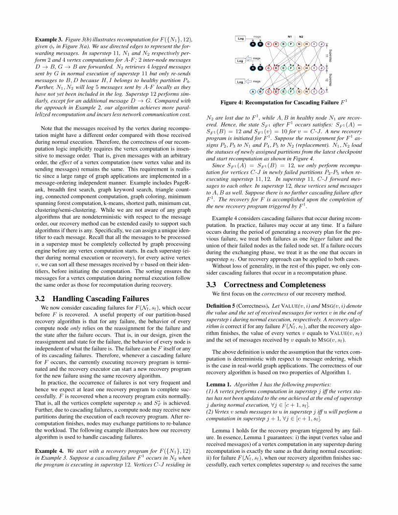
Example 4. We start with a recovery program for F ({N1}, 12)in Example 3. Suppose a cascading failure F 1 occurs in N2 whenthe program is executing in superstep 12. Vertices C-J residing in

N1 N2

Superste

p

11

Log

Superste

p

12

msgs

CA B D E F IG H J

CA B D E F IG H J

CA B D E F IG H J

Logmsgs

Log msgs

Figure 4: Recomputation for Cascading Failure F 1

N2 are lost due to F 1, while A,B in healthy node N1 are recov-ered. Hence, the state SF1 after F 1 occurs satisfies: SF1(A) =SF1(B) = 12 and SF1(v) = 10 for v = C-J . A new recoveryprogram is initiated for F 1. Suppose the reassignment for F 1 as-signs P2, P3 to N1 and P4, P5 to N2 (replacement). N1, N2 loadthe statuses of newly assigned partitions from the latest checkpointand start recomputation as shown in Figure 4.

Since SF1(A) = SF1(B) = 12, we only perform recompu-tation for vertices C-J in newly failed partitions P2-P5 when re-executing superstep 11, 12. In superstep 11, C-J forward mes-sages to each other. In superstep 12, these vertices send messagesto A,B as well. Suppose there is no further cascading failure afterF 1. The recovery for F is accomplished upon the completion ofthe new recovery program triggered by F 1.

Example 4 considers cascading failures that occur during recom-putation. In practice, failures may occur at any time. If a failureoccurs during the period of generating a recovery plan for the pre-vious failure, we treat both failures as one bigger failure and theunion of their failed nodes as the failed node set. If a failure occursduring the exchanging phase, we treat it as the one that occurs insuperstep sf . Our recovery approach can be applied to both cases.

Without loss of generality, in the rest of this paper, we only con-sider cascading failures that occur in a recomputation phase.

3.3 Correctness and CompletenessWe first focus on the correctness of our recovery method.

Definition 5 (Correctness). Let VALUE(v, i) and MSG(v, i) denotethe value and the set of received messages for vertex v in the end ofsuperstep i during normal execution, respectively. A recovery algo-rithm is correct if for any failure F (Nf , sf), after the recovery algo-rithm finishes, the value of every vertex v equals to VALUE(v, sf )and the set of messages received by v equals to MSG(v, sf ).

The above definition is under the assumption that the vertex com-putation is deterministic with respect to message ordering, whichis the case in real-world graph applications. The correctness of ourrecovery algorithm is based on two properties of Algorithm 1.

Lemma 1. Algorithm 1 has the following properties:(1) A vertex performs computation in superstep j iff the vertex sta-tus has not been updated to the one achieved at the end of superstepj during normal execution, ∀j ∈ [c+ 1, sf ].(2) Vertex v sends messages to u in superstep j iff u will perform acomputation in superstep j + 1, ∀j ∈ [c+ 1, sf ].

Lemma 1 holds for the recovery program triggered by any fail-ure. In essence, Lemma 1 guarantees: i) the input (vertex value andreceived messages) of a vertex computation in any superstep duringrecomputation is exactly the same as that during normal execution;ii) for failure F (Nf , sf), when our recovery algorithm finishes suc-cessfully, each vertex completes superstep sf and receives the same

Algorithm 2: CostSensitiveReassignInput : S, state after the failure occurs

Pf , failed partitionsI, statisticsN , a set of compute nodes

Output: φr: reassignment1 φr ←RandomAssign(Pf ,N);2 Tlow ←ComputeCost(φr, S, I);3 while true do4 φr

′ ← φr; P ← Pf ; i← 0;5 while P 6= ∅ do6 i← i+ 1;7 Li ←NextChange(φr′,P, S, I);8 foreach P ∈ Li.φ.Keys() do9 φr

′(P )← Li.φ(P );10 P ← P − {P};

11 l← argmini Li.T ime;12 if Ll.T ime < Tlow then13 for j = 1 to l do14 foreach P ∈ Lj .φ.Keys() do15 φr(P )← Lj .φ(P );

16 Tlow ← Ll.T ime;17 else18 break;

set of messages as it does at the end of superstep sf during normalexecution. These properties ensure the correctness of our approach.

Furthermore, our recovery algorithm is complete in that the re-covery logic is independent of high-level applications. That is, anynode failure can be correctly recovered using our algorithm.

Theorem 1. Our partition-based recovery algorithm is correct andcomplete.

4. REASSIGNMENT GENERATIONIn this section, we present how to generate reassignment for any

failure. Consider a failure F (Nf , sf). The reassignment for F iscritical to the overall recovery performance, i.e., the time span ofrecovery. In particular, it decides the computation and communica-tion cost during recomputation. Our objective is to find a reassign-ment that minimizes the recovery time Γ(F ).

Given the reassignment for F , the calculation of Γ(F ) is compli-cated by the fact that Γ(F ) depends not only on the reassignmentfor F , but also on the cascading failures for F and the correspond-ing reassignments. However, the knowledge of cascading failurescan hardly be obtained beforehand since F and its cascading fail-ures do not arrive as a batch but come sequentially. Hence, weseek an online reassignment generation algorithm that can react inresponse to any failure, without knowledge of future failures.

Our main insight is that when a failure (either F or its cascad-ing failure) occurs, we prefer a reassignment that can benefit theremaining recovery process for F by taking into account all thecascading failures that have already occurred. More specifically,we collect the state S after the failure occurs and measure the min-imum time Tlow required to transform from S to S∗F , i.e., the timeof performing recomputation from superstep c+1 to sf without fur-ther cascading failures. We then aim to produce a reassignment thatminimizes Tlow. Essentially, S encapsulates all the useful informa-tion about previous failures and the corresponding reassignmentsperformed, and Tlow provides a lower bound of remaining recov-ery time for F . In what follows, we introduce how to compute Tlowand then provide our cost-driven reassignment algorithm.

Algorithm 3: NextChangeInput : φr, reassignment P , a set of partitions

I, statistics N , a set of compute nodesOutput: L: exchange

1 φ← ∅; Li.T ime← +∞;2 foreach P ∈ P do3 foreach P ′ ∈ P − {P} do4 φr

′ ← φr;5 Swap φr′(P ) and φr′(P ′);6 t′ ←ComputeCost(φr′, S, I);7 if Li.T ime > t′ then8 Li.φ← {(P, φr(P ′)), (P ′, φr(P ))};9 Li.T ime← t′;

10 foreach N ∈ N − {φr(P )} do11 φr

′ ← φr; φr′(P )← N ;12 t′ ←ComputeCost(φr′, S, I);13 if Li.T ime > t′ then14 Li.φ← {(P,N)};15 Li.T ime← t′;

4.1 Estimation of TlowFor any failure, Tlow is determined by the total amount of com-

putation cost and network communication cost required during re-computation, which is formally defined as follows.

Tlow =

sf∑i=c+1

(Tp [i] +Tm [i]) (3)

where Tp [i] and Tm [i] denote the time for vertex computation andthat for inter-node message passing required in superstep i duringrecomputation, respectively.

Equation 3 ignores the downtime period for replacing failed nodesand synchronization time because they are almost invariant w.r.t.the recovery methods discussed in this paper. We also assume thecost of intra-node message passing is negligible compared withnetwork communication cost incurred by inter-node messages.

We now focus on how to compute Tp [i] and Tm [i] in Equa-tion 3. Let Si and φpi denote the state and the partition-node map-ping in the beginning of superstep i (during recomputation), respec-tively. We find that Tp [i] and Tm [i] can be computed based on Siand φpi. Therefore, we first describe how to compute Si, φpi, andthen define Tp [i] and Tm [i] based on Si, φpi.Compute Si, φpi. For i = c + 1, Sc+1 is the state right afterthe failure (either F or its cascading failure) occurs. Let ϕ be thevertex-partition mapping, φr be the reassignment for the failure,and Pf be the set of failed partitions. We have:

φpc+1(v) =

{φr(v) If ϕ(v) ∈ Pf

φp(v) Otherwise(4)

For any i ∈ (c+ 1, sf ], we have:

φpi = φpc+1, Si(v) =

{Sc+1(v) If Sc+1(v) ≥ ii− 1 Otherwise

(5)

Compute Tp [i] ,Tm [i]. We now formally define Tp [i] and Tm [i].According to the computation model in Section 2.1, computa-

tion time required in a superstep is determined by the slowest node,i.e., maximum computation time among all the nodes. Let A(i)be the set of vertices that perform computation during re-executionof superstep i. Let τ(v, i) denote the computation time of v in thenormal execution of superstep i, ϕ be the vertex-partition mapping.

Tp [i] = maxN∈N

∑τ(v,i)

{v ∈ A(i) | φpi(ϕ(v)) = N} (6)

P1

P2

P3

(a) Initial

Modification Tmin

P2 > N2, P1 > N1

P3 > N2, P1 > N1

P2 > N2

P3 > N2

P1 > N1

P2, P

3P1

N1 N2

Tmin=

Modification Tmin

P3 > N2, P1 > N1

P3 > N2

P1 > N1

P3

P1, P2N1 N2

Tmin=

1st iteration

2nd iteration

(b) Pass 1

Modification Tmin

P1 > N2, P2 > N1

P1 > N2, P3 > N1

P1 > N2 12

P2 > N1

P3 > N1

Modification Tmin

P2 > N1

P3 > N1

Modification Tmin

P2 > N1

P1

P2,P

3N1 N2

Tmin =

P1 ,P2 , P3N1 N2

Tmin =

P3 P1 ,P2N1 N2

Tmin =

1st iteration

2nd iteration

3rd iteration

(c) Pass 2

Figure 5: Example of Modifications

Due to simplicity, we assume computations for vertices in one nodeare performed sequentially. A more accurate estimation for Tp [i]can be applied if the computation within a node can be parallelizedusing machines with multithreaded and multicore CPUs.

To compute Tm [i], we adopt the Hockney’s model [11], whichestimates network communication time by the total size of inter-node messages divided by network bandwidth. Let M(i) be theset of messages forwarded when re-executing superstep i. Letm.u,m.v and µ(m) be the source vertex, destination vertex and size ofmessage m, respectively. Suppose the network bandwidth is B.

Tm [i] =∑

µ(m)/B

{m ∈M(i) | φpi(ϕ(m.u))) 6= φpi(ϕ(m.v))} (7)

Note thatA(i), τ(v, i),M(i) and µ(m) in Equation 6 and 7 canonly be obtained during the runtime execution of the application. Aperfect knowledge of these values requires a detailed bookkeepingof graph status in every superstep, which incurs high maintainencecost. Therefore, we refer to statistics (See Section 3) for approx-imation. Specifically, we can learn from Si, φpi whether a par-tition will perform computation and forward messages to anotherpartition during the re-execution of superstep i, and based on thestatistics, we know the computation cost and communication costamong these partitions in superstep c. We then approximate thecosts in superstep i by those in superstep c.

Example 5. Consider F ({N1}, 12) in Example 2 and φr in Fig-ure 5(a). Let c1 and c2 be the time for each vertex computationand that for sending an inter-node message, respectively. To com-pute Tlow under φr, we calculate the re-execution time of superstep11, 12 without further cascading failures. In both supersteps, com-putation time is 4c1 caused by P1, P2 in N1. Communication timein superstep 11 is 5c2 caused by 5 inter-node messages: 1 from P2

toP1, 4 fromP4 toP2, P3, and that in superstep 12 is 6c2 followingthe 6 cross-node edges. Hence, Tlow under φr is 8c1 + 11c2.

Theorem 2. Given a failure, finding a reassignment φr for it thatminimizes Tlow in Equation 3 is NP-hard.

Theorem 2 can be proven by reducing the graph partitioningproblem to the problem of finding reassignment with minimizedTlow. We omit proof due to space constraint.

4.2 Cost-Sensitive Reassignment AlgorithmDue to the hardness result in Theorem 2, we develop a cost-

sensitive reassignment algorithm. Before presenting our algorithm,we shall highlight the differences between our problem and tra-ditional graph partitioning problems. First and foremost, the tra-ditional graph partitioning problems focus on partitioning a staticgraph into k components with the objective of minimizing the num-ber of cross-component edges. In our case, we try to minimize theremaining recovery time Tlow. Tlow is independent of the originalgraph structure but relies on the vertex states and message-passingduring the execution period. Second, graph partitioning outputs k

components where k is predefined. On the contrary, our reassign-ment is required to dynamically allocate the failed partitions amongthe healthy nodes without the knowledge of k. Further, besides thepartitioning, we must know the node to which a failed partitionwill be reassigned. Third, traditional partitioning always requires kcomponents to have roughly equal size, while we allow unbalancedreassignment, i.e., assign more partitions to one node but fewer toanother, if a smaller value of Tlow can be achieved.

Algorithm 2 outlines our reassignment algorithm. We first gen-erate a reassignment φr by randomly assigning partitions in Pf

among compute nodes N , and then calculate Tlow under φr (line1-2). We next make a copy of φr as φr

′ and improve φr′ itera-

tively (line 3-18). In the i-th iteration, the algorithm chooses somepartitions and modifies their reassignments (line 7-9). The modifi-cation information is stored in Li. Li is in the form of (φ, T ime),where φ is a partition-node mapping recording which partition ismodified to be reassigned to which node, and T ime is Tlow underthe modified reassignment. The selected partitions are removed forfurther consideration (line 10). The iteration terminates when nomore failed partitions are left. After that, we check list L and find lsuch that Ll.T ime is minimal (line 11), i.e.,

l← arg miniLi.T ime

If Ll.T ime is smaller than Tlow achieved by the initial reassign-ment φr, we update φr by sequentially applying all the modifica-tions in L1, · · · ,Ll (line 12-16), and start another pass of itera-tions. Otherwise, we return φr as the result.

Algorithm 3 describes how to generate modification Li (line 7 inAlgorithm 2) in the i-th iteration. We focus on two types of modi-fications: i) exchanging the reassignments between two partitions;ii) changing the reassignment for one partition. Given a reassign-ment φr, NEXTCHANGE iterates over all the partitions (line 2) andfor each partition P , it enumerates all of the possible modifica-tions, i.e., exchanging the reassignment of P with another parti-tion (line 3-9) as well as assigning P to another node instead ofφr(P ) (line 10-15). NEXTCHANGE computes the correspondingTlow achieved by each modification and chooses the one with min-imized value of Tlow as the modification Li.

Example 6. Continuing from Example 5, suppose c1c2

= 1.1. Fig-ure 5(a) shows the initial reassignment with Tlow = 8c1 + 11c2.Figure 5(a) provides enumerated modifications and their Tlow inthe first pass. In iteration 1, assigning P2 to N2 achieves minimumTlow: 8c1 + 6c2. In iteration 2, we only consider modifications forP1, P3 as P1 has been considered. Exchanging reassignments forP1, P3 produces Tlow of 8c1 + 4c2. After that, all the partitionshave been considered. We apply the first two modifications to theinitial reassignment because the minimal Tlow (i.e., 8c1 + 4c2) isachieved after the second modification.

Figure 5(c) shows enumerated modifications and their Tlow inpass 2. The minimal Tlow (i.e., 12c1) in three iterations is achievedafter the first modification, which is larger than 8c1 + 4c2. Hence,

Assign

partitions

Load partitions

Perform

computation

Synchronize

checkpoint

Synchronize

superstep

Exchange

partitions

Save

checkpointRestart?

Master

Slavers

N

Y

Figure 6: Processing a Superstep in Giraph

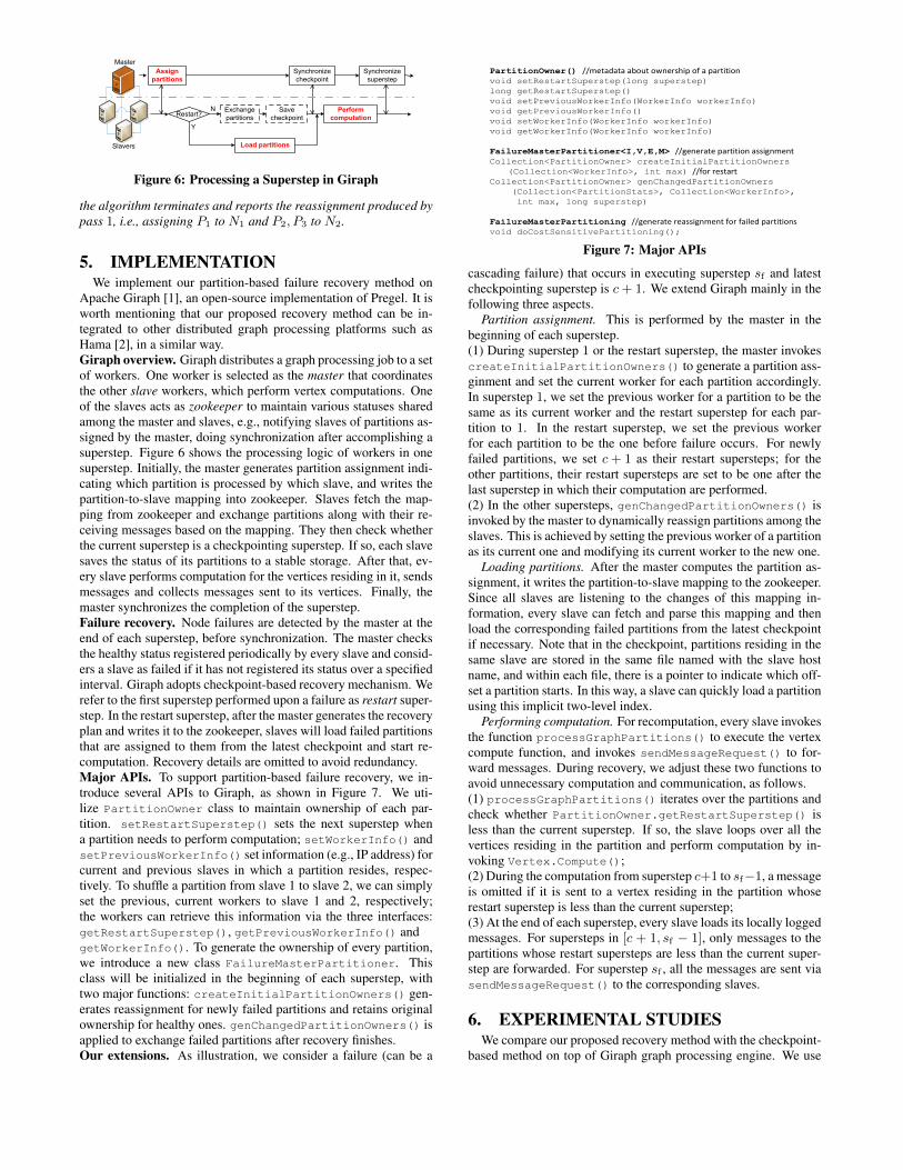
the algorithm terminates and reports the reassignment produced bypass 1, i.e., assigning P1 to N1 and P2, P3 to N2.

5. IMPLEMENTATIONWe implement our partition-based failure recovery method on

Apache Giraph [1], an open-source implementation of Pregel. It isworth mentioning that our proposed recovery method can be in-tegrated to other distributed graph processing platforms such asHama [2], in a similar way.Giraph overview. Giraph distributes a graph processing job to a setof workers. One worker is selected as the master that coordinatesthe other slave workers, which perform vertex computations. Oneof the slaves acts as zookeeper to maintain various statuses sharedamong the master and slaves, e.g., notifying slaves of partitions as-signed by the master, doing synchronization after accomplishing asuperstep. Figure 6 shows the processing logic of workers in onesuperstep. Initially, the master generates partition assignment indi-cating which partition is processed by which slave, and writes thepartition-to-slave mapping into zookeeper. Slaves fetch the map-ping from zookeeper and exchange partitions along with their re-ceiving messages based on the mapping. They then check whetherthe current superstep is a checkpointing superstep. If so, each slavesaves the status of its partitions to a stable storage. After that, ev-ery slave performs computation for the vertices residing in it, sendsmessages and collects messages sent to its vertices. Finally, themaster synchronizes the completion of the superstep.Failure recovery. Node failures are detected by the master at theend of each superstep, before synchronization. The master checksthe healthy status registered periodically by every slave and consid-ers a slave as failed if it has not registered its status over a specifiedinterval. Giraph adopts checkpoint-based recovery mechanism. Werefer to the first superstep performed upon a failure as restart super-step. In the restart superstep, after the master generates the recoveryplan and writes it to the zookeeper, slaves will load failed partitionsthat are assigned to them from the latest checkpoint and start re-computation. Recovery details are omitted to avoid redundancy.Major APIs. To support partition-based failure recovery, we in-troduce several APIs to Giraph, as shown in Figure 7. We uti-lize PartitionOwner class to maintain ownership of each par-tition. setRestartSuperstep() sets the next superstep whena partition needs to perform computation; setWorkerInfo() andsetPreviousWorkerInfo() set information (e.g., IP address) forcurrent and previous slaves in which a partition resides, respec-tively. To shuffle a partition from slave 1 to slave 2, we can simplyset the previous, current workers to slave 1 and 2, respectively;the workers can retrieve this information via the three interfaces:getRestartSuperstep(), getPreviousWorkerInfo() andgetWorkerInfo(). To generate the ownership of every partition,we introduce a new class FailureMasterPartitioner. Thisclass will be initialized in the beginning of each superstep, withtwo major functions: createInitialPartitionOwners() gen-erates reassignment for newly failed partitions and retains originalownership for healthy ones. genChangedPartitionOwners() isapplied to exchange failed partitions after recovery finishes.Our extensions. As illustration, we consider a failure (can be a

PartitionOwner() //metadata about ownership of a partition

void setRestartSuperstep(long superstep)

long getRestartSuperstep()

void setPreviousWorkerInfo(WorkerInfo workerInfo)

void getPreviousWorkerInfo()

void setWorkerInfo(WorkerInfo workerInfo)

void getWorkerInfo(WorkerInfo workerInfo)

FailureMasterPartitioner<I,V,E,M> //generate partition assignment

Collection<PartitionOwner> createInitialPartitionOwners

(Collection<WorkerInfo>, int max) //for restart

Collection<PartitionOwner> genChangedPartitionOwners

(Collection<PartitionStats>, Collection<WorkerInfo>,

int max, long superstep)

FailureMasterPartitioning //generate reassignment for failed partitions

void doCostSensitivePartitioning();

Figure 7: Major APIs

cascading failure) that occurs in executing superstep sf and latestcheckpointing superstep is c+ 1. We extend Giraph mainly in thefollowing three aspects.

Partition assignment. This is performed by the master in thebeginning of each superstep.(1) During superstep 1 or the restart superstep, the master invokescreateInitialPartitionOwners() to generate a partition ass-ginment and set the current worker for each partition accordingly.In superstep 1, we set the previous worker for a partition to be thesame as its current worker and the restart superstep for each par-tition to 1. In the restart superstep, we set the previous workerfor each partition to be the one before failure occurs. For newlyfailed partitions, we set c+ 1 as their restart supersteps; for theother partitions, their restart supersteps are set to be one after thelast superstep in which their computation are performed.(2) In the other supersteps, genChangedPartitionOwners() isinvoked by the master to dynamically reassign partitions among theslaves. This is achieved by setting the previous worker of a partitionas its current one and modifying its current worker to the new one.

Loading partitions. After the master computes the partition as-signment, it writes the partition-to-slave mapping to the zookeeper.Since all slaves are listening to the changes of this mapping in-formation, every slave can fetch and parse this mapping and thenload the corresponding failed partitions from the latest checkpointif necessary. Note that in the checkpoint, partitions residing in thesame slave are stored in the same file named with the slave hostname, and within each file, there is a pointer to indicate which off-set a partition starts. In this way, a slave can quickly load a partitionusing this implicit two-level index.

Performing computation. For recomputation, every slave invokesthe function processGraphPartitions() to execute the vertexcompute function, and invokes sendMessageRequest() to for-ward messages. During recovery, we adjust these two functions toavoid unnecessary computation and communication, as follows.(1) processGraphPartitions() iterates over the partitions andcheck whether PartitionOwner.getRestartSuperstep() isless than the current superstep. If so, the slave loops over all thevertices residing in the partition and perform computation by in-voking Vertex.Compute();(2) During the computation from superstep c+1 to sf−1, a messageis omitted if it is sent to a vertex residing in the partition whoserestart superstep is less than the current superstep;(3) At the end of each superstep, every slave loads its locally loggedmessages. For supersteps in [c + 1, sf − 1], only messages to thepartitions whose restart supersteps are less than the current super-step are forwarded. For superstep sf , all the messages are sent viasendMessageRequest() to the corresponding slaves.

6. EXPERIMENTAL STUDIESWe compare our proposed recovery method with the checkpoint-

based method on top of Giraph graph processing engine. We use

380

385

390

395

400

405

410

415

420

2 4 6 8 10 12 14 16 18

Runn

ing T

ime

(s)

Superstep

CBRPBR

(a) Logging Overhead

0 500

1000 1500 2000 2500 3000 3500 4000 4500 5000

11 12 13 14 15 16 17 18 19

Reco

very

Tim

e (s

)

Failed Superstep

CBRPBR

(b) Single Node Failure

0

500

1000

1500

2000

2500

3000

1 2 3 4 5

Reco

very

Tim

e (s

)

# of Failed Workers

CBRPBR

(c) Multiple Node Failure

0

1000

2000

3000

4000

5000

6000

7000

8000

11 12 13 14 15 16 17 18

Reco

very

Tim

e (s

)

Failed Superstep

CBRPBR

(d) Cascading Failure

Figure 8: k-means

0

20

40

60

80

100

2 4 6 8 10 12 14 16 18

Runn

ing T

ime

(s)

Superstep

CBRPBR

(a) Logging Overhead

0

100

200

300

400

500

600

700

800

11 12 13 14 15 16 17 18 19

Reco

very

Tim

e (s

)

Failed Superstep

CBRPBR

(b) Single Node Failure

50 100 150 200 250 300 350 400 450 500

1 2 3 4 5

Reco

very

Tim

e (s

)

# of Failed Workers

CBRPBR

(c) Multiple Node Failure

0

200

400

600

800

1000

1200

1400

11 12 13 14 15 16 17 18

Reco

very

Tim

e (s

)

Failed Superstep

CBRPBR

(d) Cascading Failure

Figure 9: Semi-clustering

the latest version-1.0.0 of Giraph that is available in [1].

6.1 Experiment SetupThe experimental study was conducted on our in-house clus-

ter. The cluster consists of 72 compute nodes, each of which isequipped with one Intel X3430 2.4GHz processor, 8GB of mem-ory, two 500GB SATA hard disks. All the nodes are hosted on tworacks. The nodes within one rack are connected via 1 Gbps switchand the two racks are connected via a 10 Gbps cluster switch. Oneach compute node, we installed CentOS 5.5 operating system,Java 1.6.0 with a 64-bit server VM and Hadoop 0.20.203.03. Gi-raph runs as a MapReduce job on top of Hadoop, hence we madethe following changes to the default Hadoop configurations: (1) thesize of virtual memory for each task was set to 4GB; (2) each nodewas configured to run one map task. By default, we chose 42 nodesout of the 72 nodes for the experiments and among them, one nodeacted as the master running Hadoop’s NameNode and JobTrackerdaemons while the other 41 nodes ran TaskTracker daemons andGiraph jobs. Among the 41 nodes that ran Giraph jobs, one nodeacted as the master and zookeeper, and the others were slaves.

6.2 Benchmark Tasks and DatasetsWe study the failure recovery over three benchmark tasks: k-

means, semi-clustering [20] and PageRank.• k-means. We implement k-means in Giraph4. In our experi-ments, we set k = 100.• Semi-clustering. A semi-cluster in a social graph consists of agroup of people who interact frequently with each other and lessfrequently with others. We port the implementation in Hama [2]into Giraph. We use the same parameter values as in Hama, i.e.,each cluster contains at most 100 vertices, a vertex is involved in atmost 10 clusters, and the boundary edge score factor is set to 0.2.• PageRank. The PageRank algorithm is contained in the Giraphpackage and we simply use it to run PageRank tasks.

Without loss of generality, we run all the tasks for 20 supersteps,and perform a checkpoint at the beginning of superstep 11. For allexperiments, the results are averaged over ten runs.

We evaluate benchmark tasks over one vector dataset and tworeal-life social network graphs (Table 2 provides dataset details andthe two graph datasets are downloaded from the website5).3http://hadoop.apache.org/4https://github.com/tmalaska/Giraph.KMeans.Example/5http://snap.stanford.edu/data/index.html

Table 2: Dataset DescriptionDataset Data Size #Vertices #Edges #PartitionsForest 2.7G 58,101,200 0 160LiveJournal 1.0G 3,997,962 34,681,189 160Friendster 31.16G 65,608,366 1,806,067,135 160

• Forest. Forest dataset6 predicts forest cover type from carto-graphic variables. It originally contains 580K objects, each of whichis associated with 10 integer attributes. To evaluate the perfor-mance on large datasets, we increase the size of Forest to 58,101,200while maintaining the same distribution of values over each dimen-sion using the data generator from [19]. We use this dataset toevaluate the execution of k-means tasks.• LiveJournal. LiveJournal is an online social networking andjournaling service that enables users to post blogs, journals, anddairies. It contains more than 4 million vertices (users) and about70 million directed edges (friendships between users). We use thisdataset to evaluate the execution of semi-clustering tasks.• Friendster. Friendster is an online social networking and gamingservice. It contains more than 60 millions vertices and 1 billionedges. We use it to evaluate the execution of PageRank tasks.

We compare our proposed partition-based recovery method (PBR)with the checkpoint-based recovery method (CBR) over two met-rics: recovery time and communication cost.

6.3 k-meansWe first study the overhead of logging outgoing messages at the

end of each superstep in PBR. Figure 8(a) shows the running time.PBR takes almost the same time as CBR. The reason is that in k-means tasks, there does not exist any outgoing messages amongdifferent vertices, and in this case, PBR performs exactly the sameas CBR during normal execution. Another interesting observationis that the checkpointing superstep 10 does not incur higher runningtime compared with other supersteps. This is because comparedwith computing the new belonging cluster for each observation, thetime of doing checkpointing is negligible.

We then evaluate the performance of recovery methods for singlenode failures by varying the failed superstep from 11 to 19. Figure8(b) plots the results. The recovery time of both CBR and PBR in-creases linearly when the failed superstep varies. Since there are nomessages passing among different workers, computing the new be-longing clusters for failed partitions can be accelerated by using all

6http://archive.ics.uci.edu/ml/datasets/Covertype

20 40 60 80

100 120 140 160 180 200

1 2 3 4 5

Com

mun

icat

ion

Cos

t (G

B)

# of Failed Workers

CBRPBR

(a) Multiple Node Failure

0

100

200

300

400

500

600

11 12 13 14 15 16 17 18

Com

mun

icatio

n Co

st (G

B)

Failed Superstep

CBRPBR

(b) Cascading Failure

Figure 10: Communication Cost of Semi-clustering

available workers, i.e., recomputation is parallelized over 40 work-ers for recovery. We find that PBR outperforms CBR by a factorof 12.4 to 25.7 and there is an obvious gain when the failed super-step increases. The speedup is less than 40x due to the overhead ofloading the checkpoint in the beginning of a recovery.

Next, we investigate the performance of recovery methods formultiple node failures. The number of failed nodes is varied from1 to 5 and the failed superstep is set to 15. Figure 8(c) plots the re-sults. When the number of failed nodes increases, the recovery timeincreases linearly for PBR while that remains constant for CBR. Nomatter how many nodes fail, CBR will redo all computation fromthe latest checkpoint, while PBR recomputes the new belongingclusters for observations in the failed nodes and hence the recov-ery time becomes longer for a larger number of failed nodes. Onaverage, PBR outperforms CBR by a factor of 6.8 to 23.9.

Finally, we focus on cascading failure by setting the first failedsuperstep to 19 and varying the second failed superstep from 11 to18. Figure 8(d) plots the results. When the second failed superstepincreases, the recovery time increases linearly for both CBR andPBR. On average, PBR can reduce recovery time by a factor of23.8 to 26.8 compared with CBR.

6.4 Semi-clusteringFigure 9(a) plots the running time of each superstep for semi-

clustering. PBR takes slightly longer time than CBR during nor-mal execution. This is because compared with the computationand communication costs, the overhead of logging outgoing mes-sages to local disks is relatively insignificant. Moreover, in semi-clustering, the size of each message from a vertex to its neighborsincreases linearly with the superstep. Hence, both CBR and PBRruns slower in larger supersteps. In superstep 10, there is an obvi-ous increment in the running time due to performing a checkpoint.

We evaluate the performance of recovery methods for single nodefailures, multiple node failures and cascading failures using thesame settings as k-means. Figure 9(b), 9(c), 9(d) show the re-spective results. Basically, the trends of the running time of PBRand CBR in semi-clustering follows those in k-means. Specifically,PBR outperforms CBR by a factor of 9.0 to 15.3 for single nodefailures, by a factor of 13.1 to 5.8 for multiple node failures, and bya factor of 14.3 to 16.6 for cascading failures.

Besides the benefit of parallelizing computation, we also showthe communication cost incurred by PBR and CBR in Figure 10.Since messages sent to the vertices residing in the healthy nodescan be omitted in PBR, we observe that in multiple node failure,PBR incurs 6.5 to 37.9 times less communication cost than CBR.For cascading failures, PBR can reduce communication cost by afactor of 37.1 compared with CBR.

6.5 PageRankTo study the logging overhead for PageRank tasks, we report

the running time of every superstep in Figure 11(a). Comparedwith k-means and semi-clustering, PBR takes slightly more timethan CBR in PageRank. This is because PageRank is evaluatedover the Friendster dataset which has a power-law link distribution

Table 3: Parameter Ranges for Simulation StudyParameter Description Range

n number of failed partitions 20, 40, 50m number of healthy nodes 20, 40, 50k number of partitions (or healthy nodes)

with high communication cost2, 4, 8

γ comp-comm-ratio 0.1, 1, 10

and each superstep involves a huge number of forwarding messagesthat should be logged locally via disk I/O. However, the overheadis still negligible, only 3% increase in running time. Due to doingcheckpointing, there is an obvious increment of running time in su-perstep 10. In each superstep, the worker basically does the sametask and hence the running time of each superstep almost remainsthe same. We also evaluate the performance of recovery methodsfor single node failures, multiple node failures and cascading fail-ures. Figure 11(b), 11(c), 11(d) provide the recovery time, respec-tively. Figure 12 shows the corresponding communication cost.The performance of PBR and CBR follow the same trends as thosein semi-clustering and k-means tasks. This further verifies the ef-fectiveness of PBR, which parallelizes computation and eliminatesunnecessary computation and communication cost.

6.6 Simulation StudyWe perform a simulation study to evaluate the effectiveness and

efficiency of our cost-sensitive reassignment algorithm COSTSENin partition-based recovery. As a comparison, we consider a ran-dom approach RANDOM by balancing computation among the nodes.Data preparation. We investigate the effect of the following pa-rameters that potentially affect the performance of the reassignmentalgorithms:• n: the number of failed partitions•m: the number of healthy compute nodes• computation cost per failed partition during recovery• communication cost between every two failed partitions duringrecovery• communication cost between failed partitions and healthy com-pute nodes during recovery

We generate communication cost by simulating two categories ofgraph partitioning, random-partitioning and well-partitioning. Inrandom-partitioning, there is no obvious difference in the connec-tions of two partitions lying in the same node or across two nodes;in well-partitioning, the number of edges connecting two partitionswithin the same node is much larger than that across two nodes. Forsimulation, we generate communication cost using two distribu-tions uniformly-distributed and well-distributed corresponding torandom-partitioning and well-partitioning, as follows.

1) In uniformly-distributed, the communication cost between twofailed partitions and that between a healthy node and a failed parti-tion, is uniformly drawn from the range [1, low].

2) In well-distributed, for each failed partition, we randomly se-lect k failed partitions. The communication cost from the parti-tion to each of the selected ones is uniformly drawn from range[1, high], and that from the partition to any other failed partitionis uniformly drawn from range [1, low]. The communication costbetween a partition and healthy node is generated in the same way.By default, we set p, low, high to 0.6, 100, 40000, respectively.

We generate comparable computation cost for each failed parti-tion based a comp-comm-ratio, γ. Let SP be the total communica-tion cost from healthy nodes to a failed partition P . We use γ toadjust the ratio between the computation cost of P and SP . Thecomputation cost of P is randomly drawn from the range [1, γSP ].A larger γ implies that the job is more computation-intensive. Ta-ble 3 summarizes the ranges of our tuning parameters. Unless oth-erwise specified, we use the underlined default values.

320

340

360

380

400

420

2 4 6 8 10 12 14 16 18

Runn

ing

Tim

e (s

)

Superstep

CBRPBR

(a) Logging Overhead

0

500

1000

1500

2000

2500

3000

3500

4000

11 12 13 14 15 16 17 18 19

Reco

very

Tim

e (s

)

Failed Superstep

CBRPBR

(b) Single Node Failure

0

500

1000

1500

2000

2500

3000

1 2 3 4 5

Reco

very

Tim

e (s

)

# of Failed Workers

CBRPBR

(c) Multiple Node Failure

0

1000

2000

3000

4000

5000

6000

7000

11 12 13 14 15 16 17 18

Reco

very

Tim

e (s

)

Failed Superstep

CBRPBR

(d) Cascading Failure

Figure 11: PageRank

20 40 60 80

100 120 140 160 180 200

1 2 3 4 5

Com

mun

icat

ion

Cos

t (G

B)

# of Failed Workers

CBRPBR

(a) Multiple Node Failure

50 100 150 200 250 300 350 400 450 500

11 12 13 14 15 16 17 18

Com

mun

icat

ion

Cos

t (G

B)

Failed Superstep

CBRPBR

(b) Cascading Failure

Figure 12: Communication Cost of PageRank

Measure. We measure the performance of reassignment algorithmsvia five metrics: maximum computation cost (CompCost), totalinter-node communication cost (CommCost), sum of CompCostand CommCost (TotalCost), running time and the number of nodesto which failed partitions are reassigned. All the costs are measuredin seconds by default.Effects of comp-comm-ratio. Table 4 shows the results of COST-SEN and RANDOM by varying γ in uniformly-distributed scenario.On average, COSTSEN produces reassignments with lower Total-Cost and CommCost than RANDOM over all the ratios. For γ =0.1, COSTSEN outperforms RANDOM with 2x lower TotalCost andCommCost. As γ increases, the advantage of COSTSEN in Total-Cost and CommCost becomes less significant. The reason is thata larger γ makes the job more computation-intensive; this requiresmore nodes to parallelize the computation, while CommCost canhardly be reduced due to the uniform distribution. For smaller γ(e.g., 0.1), COSTSEN assigns failed partitions to a small numberof nodes (< 5) due to insignificant CompCost, hence it reports re-assignments with higher CompCost than RANDOM. For larger γ(e.g., 10), COSTSEN performs similarly as RANDOM in terms ofthe three costs, but it requires 2x fewer nodes for recovery. Thissaving is desirable in practice. We observe similar results for thewell-distributed scenario and omit the results to avoid duplication.Effects of High Communication Partition (Healthy Node) Num-ber. Table 5 shows the results of both methods when we vary thenumber of partitions (nodes) with high communication cost (k).For all values of k, COSTSEN outperforms RANDOM with 2x lowerTotalCost and CommCost. COSTSEN produces reassignments withhigher CompCost which is relatively insignificant compared withCommCost. Furthermore, COSTSEN always involves fewer nodesfor recovery. For k = 10, it uses 15x fewer nodes than RANDOM.Effects of the number of failed partitions. Table 6 provides theresults by varying the number of failed partitions (n). For eachn, COSTSEN outperforms RANDOM by 2.5x lower TotalCost andCommCost. Again, the reassignments reported by COSTSEN re-quire higher CompCost, which is much smaller than CommCost.Furthermore, COSTSEN uses 3x fewer nodes for recovery. Fig-ure 13(a) shows the running time of COSTSEN. It requires lessthan 250ms to generate reassignments. The running time increasesquadratically with the number of failed partitions.Effects of the number of healthy nodes. Table 7 provides theresults by varying the number of healthy nodes (m). COSTSENproduces reassignments with 3x lower TotalCost and CommCostover all values of m. Furthermore, it employs fewer healthy nodes

0

50

100

150

200

250

300

10 20 30 40 50

Run

ning

Tim

e (s

)

# of Partitions

PBR

(a) # of Failed Partitions

0

50

100

150

200

250

300

10 20 30 40 50

Run

ning

Tim

e (s

)

# of Compute Nodes

PBR

(b) # of Healthy Nodes

Figure 13: Running Time (well-distributed)

Table 4: Effects of Comp-comm-ratio γ (uniformly-distributed)γ 0.1 1 10

RANDOM COSTSEN RANDOM COSTSEN RANDOM COSTSENCompCost 0.4 8.2 3.9 5.8 38.9 38.9CommCost 152.6 75.2 152.4 143.5 152.6 147.1TotalCost 153.0 83.4 156.3 149.3 191.5 186.0Used nodes 40 1 40 19.9 40 24.1

Table 5: Effects of the Number of Partitions (or Healthy Nodes) withHigh Communication Cost k (well-distributed)k 2 4 8

RANDOM COSTSEN RANDOM COSTSEN RANDOM COSTSENCompCost 3.9 17.4 3.9 46.0 3.8 76.7CommCost 1603.5 690.5 2830.1 1422.5 5190.9 2558.8TotalCost 1607.4 707.9 2834.0 1468.5 5194.7 2635.5Used nodes 40 11.75 40 7.63 40 2.79

for recovery. For larger m (e.g., 40, 50), the number of nodes in-volved in the reassignments from COSTSEN is 3x fewer than RAN-DOM. Figure 13(b) shows the running time of COSTSEN. The run-ning time increases linearly with the number of healthy nodes. Form = 50, COSTSEN generates reassignments over 40 nodes within250ms.Summary. Our simulation study show that the cost-sensitive re-assigning algorithm achieves 2x speedup in our partition-based re-covery framework compared with random assignment. It also out-performs random approach by wisely choosing a smaller number ofcompute nodes to handle failed partitions. Furthermore, our reas-signing algorithm is efficient; the running time grows quadraticallywith the number of failed partitions and linearly with the numberof healthy nodes.

7. RELATED WORKDesigning efficient failure recovery methods has long been a

goal of distributed systems. As our proposed approach acceler-ates the failure recovery by parallelizing the re-execution of failedgraph partitions according to a communication and computationcost model, we split the discussion on the existing work on fail-ure recovery in distributed graph processing systems into two cat-egories: (i) methods for accelerating the failure recovery and (ii)graph partitioning methods.Accelerating failure recovery. Failure recovery approaches aretypically split into three categories: checkpoint-based, log-basedand hybrid approaches [9]. Most popular distributed graph process-ing systems such as Giraph [1], GraphLab [18], PowerGraph [10],GPS [22], Mizan [14] adopt checkpoint-based recovery. Pregel [20]proposes confined recovery which is a hybrid mechanism of the

Table 6: Effects of the Number of Partitions n (well-distributed)n 20 40 50

RANDOM COSTSEN RANDOM COSTSEN RANDOM COSTSENCompCost 3.7 14.7 3.8 17.8 4.6 18.8CommCost 775.3 291.9 1605.2 689.0 2005.0 876.9TotalCost 779.0 306.6 1609.0 706.8 2009.6 895.7Used nodes 20 7.05 40 11.69 40 15.19

Table 7: Effects of the Number of Healthy Nodes m (well-distributed)m 20 40 50

RANDOM COSTSEN RANDOM COSTSEN RANDOM COSTSENCompCost 5.9 20.5 3.9 15.6 3.8 16.5CommCost 1463.3 572.1 1582.0 686.8 1617.9 695.8TotalCost 1469.2 592.6 1585.9 702.4 1621.7 712.3Used nodes 20 10.21 40 12.27 40 12.97

checkpoint-based and log-based recovery. Specifically, only thenewly-added node that substitutes the failed one has to rollback andrepeats the computations from the latest checkpoint. GraphX [26]adopts log (called lineage) based recovery, and utilizes resilientdistributed datasets (RDD) to speedup failure recovery. However,when a node fails, graph data lying in this node still need to be re-covered. Checkpointing and logging operations are the backboneof recovery methods [5, 6, 7]. Much work has focused on acceler-ating them has long been a target for optimizations [9]. However,our proposed parallel recovery method is orthogonal to most of theworks that accelerate the checkpoint-based or the log-based recov-ery. Location and replication independent recovery proposed byBratsberg et al. employed replicas for recovery [8]. The algorithmpartitions the data into fragments and replicates fragments amongmultiple nodes which can takeover in parallel upon failures. How-ever, the recovery task for the failed node is still performed in a cen-tralized manner after the node finishes internal recovery. Instead,we focus on accelerating the task of recovering by parallelizing thecomputations required to recompute the lost data. Another recov-ery method that presents similarities with ours is present in RAM-Cloud [21]. RAMCloud backs up the data across many distributednodes, and during recovery, it reconstructs in parallel the lost data.However, as RAMCloud is a distributed storage, it does not needto track the dependencies among the scattered data. In contrast,in distributed processing systems, understanding how the programdependencies affect both the communication and the computationtime is of utmost importance [4].Graph partitioning. METIS [13], which performs offline par-titioning of a distributed unstructured graph, is most relevant toour approach for partitioning the failed subgraph. Several exten-sions have been proposed such as for power-law graphs [3], multi-threaded graph partitioning [15] and dynamic multi-constraint graphpartitioning [23]. In practice, it has been adopted in other dis-tributed graph processing systems such as PowerGraph. However,METIS does not partition based on a cost model that includes bothcommunication and computation.

8. CONCLUSIONThis paper presents a novel partition-based recovery method to

parallelize failure recovery processing. Different from traditionalcheckpoint-based recovery, our recovery method distributes the re-covery tasks to multiple compute nodes such that the recovery pro-cessing can be executed concurrently. Because partition-based fail-ure recovery problem is NP-Hard, we use a communication andcomputation cost model to split the recovery among the computenodes. We implement our recovery method on the widely used Gi-raph system and observe that our proposed parallel failure recoverymethod outperforms existing checkpoint-based recovery methodsby up to 30 times when using 40 compute nodes.

AcknowledgmentThis work was supported by the National Research Foundation,Prime Minister’s Office, Singapore under Grant No. NRF-CRP8-2011-08. We thank Xuan Liu for his contributions on the earlierwork of this paper.

9. REFERENCES[1] http://giraph.apache.org/.[2] https://hama.apache.org/.[3] A. Abou-Rjeili and G. Karypis. Multilevel algorithms for partitioning

power-law graphs. In IPDPS, 2006.[4] P. Alvaro, N. Conway, J. M. Hellerstein, and D. Maier. Blazes:

Coordination analysis for distributed programs. In ICDE, pages52–63, 2014.

[5] J. F. Bartlett. A nonstop kernel. In SOSP, pages 22–19, 1981.[6] A. Borg, J. Baumbach, and S. Glazer. A message system supporting

fault tolerance. In SOSP, pages 90–99, 1983.[7] A. Borg, W. Blau, W. Graetsch, F. Herrmann, and W. Oberle. Fault

tolerance under unix. In ACM Trans. Comput. Syst., pages 1–24,1989.

[8] S. E. Bratsberg, S.-O. Hvasshovd, and O. Torbjørnsen. Location andreplication independent recovery in a highly available database. InBNCOD, pages 23–37, 1997.

[9] E. N. M. Elnozahy, L. Alvisi, Y.-M. Wang, and D. B. Johnson. Asurvey of rollback-recovery protocols in message-passing systems.ACM Comput. Surv., 34(3), 2002.

[10] J. E. Gonzalez, Y. Low, H. Gu, D. Bickson, and C. Guestrin.Powergraph: Distributed graph-parallel computation on naturalgraphs. In OSDI, pages 17–30, 2012.

[11] R. W. Hockney. The communication challenge for mpp: Intelparagon and meiko cs-2. In Parallel Computing, pages 389–398,1994.

[12] D. Jiang, G. Chen, B. C. Ooi, K.-L. Tan, and S. Wu. epic: anextensible and scalable system for processing big data. In PVLDB,pages 541–552, 2014.

[13] G. Karypis and V. Kumar. Metis - unstructured graph partitioning andsparse matrix ordering system, version 2.0. Technical report, 1995.

[14] Z. Khayyat, K. Awara, A. Alonazi, H. Jamjoom, D. Williams, andP. Kalnis. Mizan: a system for dynamic load balancing in large-scalegraph processing. In EuroSys, pages 169–182, 2013.

[15] D. LaSalle and G. Karypis. Multi-threaded graph partitioning. InIPDPS, 2013.

[16] F. Li, B. C. Ooi, M. T. zsu, and S. Wu. Distributed data managementusing mapreduce. In ACM Comput. Surv., page 31, 2014.

[17] Y. Low, J. Gonzalez, A. Kyrola, D. Bickson, C. Guestrin, and J. M.Hellerstein. Graphlab: A new framework for parallel machinelearning. In UAI, 2010.

[18] Y. Low, J. Gonzalez, A. Kyrola, D. Bickson, C. Guestrin, and J. M.Hellerstein. Distributed graphlab: A framework for machine learningin the cloud. In PVLDB, pages 716–727, 2012.

[19] W. Lu, Y. Shen, S. Chen, and B. C. Ooi. Efficient processing of knearest neighbor joins using mapreduce. In PVLDB, pages1016–1027, 2012.

[20] G. Malewicz, M. H. Austern, A. J. C. Bik, J. C. Dehnert, I. Horn,N. Leiser, and G. Czajkowski. Pregel: a system for large-scale graphprocessing. In SIGMOD, pages 135–146, 2010.

[21] D. Ongaro, S. M. Rumble, R. Stutsman, J. Ousterhout, andM. Rosenblum. Fast crash recovery in ramcloud. In SOSP, pages29–41, 2011.

[22] S. Salihoglu and J. Widom. Gps: a graph processing system. InSSDBM, page 22, 2013.

[23] K. Schloegel, G. Karypis, and V. Kumar. Parallel static and dynamicmulti-constraint graph partitioning. In CCPE, pages 219–240, 2002.

[24] B. Shao, H. Wang, and Y. Li. Trinity: A distributed graph engine on amemory cloud. In SIGMOD, pages 505–516, 2013.

[25] L. G. Valiant. A bridging model for parallel computation. InCommun. ACM, pages 103–111, 1990.

[26] R. S. Xin, J. E. Gonzalez, M. J. Franklin, and I. Stoica. Graphx: aresilient distributed graph system on spark. In GRADES, page 2,2013.