fast orthogonal sparse approximation algorithms over local … · fast orthogonal sparse...

appor t de r ech er ch e

ISSN

0249

-639

9IS

RNIN

RIA/

RR--7

483-

-FR+

ENG

Domaine 4

INSTITUT NATIONAL DE RECHERCHE EN INFORMATIQUE ET EN AUTOMATIQUE

Fast orthogonal sparse approximation algorithmsover local dictionaries

Boris Mailhé — Rémi Gribonval — Pierre Vandergheynst — Frédéric Bimbot

N° 7483December 2010

Centre de recherche INRIA Rennes – Bretagne AtlantiqueIRISA, Campus universitaire de Beaulieu, 35042 Rennes Cedex

Téléphone : +33 2 99 84 71 00 — Télécopie : +33 2 99 84 71 71

Fast orthogonal sparse approximation

algorithms over local dictionaries

Boris Mailhe , Remi Gribonval , Pierre Vandergheynst∗ , FredericBimbot†

Domaine : Perception, cognition, interactionEquipe-Projet METISS

Rapport de recherche n 7483 — December 2010 — 34 pages

Abstract: In this work we present a new greedy algorithm for sparse approxi-mation called LocOMP. LocOMP is meant to be run on local dictionaries madeof atoms with much shorter supports than the signal length. This notably en-compasses shift-invariant dictionaries and time-frequency dictionaries, be theymonoscale or multiscale. In this case, very fast implementations of MatchingPursuit are already available. LocOMP is almost as fast as Matching Pursuitwhile approaching the signal almost as well as the much slower OrthogonalMatching Pursuit.

Key-words: sparse approximation, greedy algorithms, shift invariance, Or-thogonal Matching Pursuit

This work was supported in part by Agence Nationale de la Recherche (ANR), projectECHANGE (ANR-08-EMER-006) and by the EU FET-Open project FP7-ICT-225913-SMALL.

∗ Ecole Polytechnique Federale de Lausanne, Switzerland† CNRS, UMR 6073 IRISA

Approximations parcimonieuses orthogonales

rapides pour dictionnaires locaux

Resume : Ce rapport presente un nouvel algorithme glouton d’approximationparcimonieuse nomme LocOMP. LocOMP est concu pour etre utilise sur desdictionnaires locaux composes d’atomes de supports courts par rapport a lalongueur du signal. Ce ca comprend notmment les dictionnaires invariants partranslation et temps-frequence, qu’ils soient mono ou multi-echelles. Dans cecas, on connaıt des implementations rapides de Matching Pursuit (MP). Lo-cOMP est presque aussi rapide que MAtching Pursuit tout en calculant un ap-proximation presque aussi bonne que le bien plus couteux Orthogonal MatchingPursuit.

Mots-cles : approximation parcimonieuse, algorithmes gloutons, invariancepar translation, Orthogonal Matching Pursuit

Fast OMP over local dictionaries 3

1 Introduction

One basis is not enough to represent certain kinds of signals. For example,music is known to be well represented by time-frequency decompositions, butwhich window length to choose? There are longer and shorter notes, and insidea note played by a free oscillation instrument such as a guitar or piano there isa short attack followed by a long relaxation. If one can find a proper basis torepresent each of those phenomena, then one would like to use the union of allthese bases to represent the whole signal. This union of bases is not a basis itselfbut a redundant dictionary Φ ∈ RN×D with D > N : given a signal s ∈ RN ,there are infinitely many possible choices of coefficients x ∈ RD that decomposes as s = Φx. Sparsity has been proposed as a way to solve the ambiguity ofsuch redundant models by selecting the decomposition that contains the fewestnon-zero coefficients.

Local dictionaries The length of the signal is chosen by the user and onlylimited by the devices sensing and recording it, but the observed phenomenacan have their own characteristic durations. So one can commonly find signalscomposed of several events that are each much shorter that the whole signal.This is typically the case in music, where a single signal will cover a whole piecemade of much shorter notes. Good dictionaries to model such a signal will alsobe composed of short atoms, each atom or a few of them trying to match oneof the phenomena.

Definition 1. Let Φ be a dictionary of size D × L. Φ is said to be local if all

its atoms ϕ are null outside of a support interval supp(ϕ) of length L � N .

Common dictionaries such as the Gabor dictionary associated with ShortTerm Fourier Transform (STFT) are local dictionaries. Shift-invariant dictio-naries are the most employed class of local dictionaries: those are made of a fewpatterns of length L that are repeated all over the signal support.

The problems that require local dictionaries typically involve large dimen-sions: the signal can contain several millions of samples and the dictionary evenmore atoms. Most known sparse approximation algorithms are too complex tobe applied to such large problems.

Scope of the paper This article explores how the locality hypothesis can beexploited to accelerate existing sparse approximation algorithms or to proposenew ones. It is focused on Matching Pursuit and Orthogonal Matching Pursuit.A fast implementation of MP is already available for shift-invariant dictionaries[1] but MP has been observed to compute significantly worse approximationsthan OMP. The aim of this work is to try to provide an implementation ofOMP as close as possible to the complexity of MP. As structural properties ofOMP make it impossible to reach the complexity of MP on local dictionaries,we propose a new algorithm called LocOMP that is only slightly less efficientthan OMP but can run almost as fast as MP.

RR n�7483


Organisation Section 2 reviews existing sparse approximation algorithmswith a strong emphasis on greedy algorithm, their detailed complexity and fastimplementation with local dictionaries. Section D presents possible accelera-tions to OMP implementation in the local case. Even with those accelerationsOMP remains much more expensive than MP.

Section 4 introduces the main contribution of this paper: the new algorithmLocOMP. The behaviour of LocOMP is close to OMP but it enables the sameaccelerations as MP. Section 6 presents experimental evaluations of Matlab im-plementations of the presented algorithms on music signals. These experimentsshow that LocOMP can achieve the same performance as OMP within the sameorder of computation time as MP. Section 8 presents future possible extensionsand theoretical developments of this work.

2 State of the art: sparse approximation algo-

rithms

In this section we briefly review some of the most common greedy algorithmswith a strong emphasis on their complexity. Let s be a signal of length Nand Φ a dictionary of size N × D. Φ is redundant if D > N and we defineits redundancy factor α = D

N. A signal s is said to be sparse over Φ if s can

be approached closely by an decomposition Φx where x contains few non-zerocoefficients:

s = Φx + r (1)

‖r‖2 � ‖s‖2 (2)

‖x‖0 � N (3)

with ‖x‖0 =∑D

d=1 x0d the number of non-zero coefficients in x. The columns of

Φ are called atoms. The problem is to find the sparse decomposition among allthe possible ones.

Problem 1. Given a signal s and a dictionary Φ and an allowed sparsity level

K, find the coefficients x that minimize

x = argmin‖x‖0≤K ‖s − Φx‖22 (4)

The sparse approximation problem (4) is proved to be NP-Hard [2]. Yetmany suboptimal algorithms have been proposed which can compute a closeapproximation within reasonable time.

2.1 `p minimization

The `0 sparsity measure has very bad properties for numerical optimization: itis not convex, not differentiable and piecewise constant. `p minimization algo-rithms replace the `0 measure by other constraints that are easier to optimize,often `p pseudo norms with 0 < p ≤ 1.

RR n�7483


`p minimization is easier to compute than `0 from a mathematical point ofview. `p pseudo-norms are continuous and piecewise differentiable so variationalapproaches can lead to a local minimum. In the special case of P = 1, the normis even convex, so there is unique local minimum and there are algorithms tofind it. However those approaches remain costly, especially when dealing withlarge data. In fact, even if the final result is sparse, intermediate iterations of`p minimization algorithms involve computations with a non-sparse x.

2.2 Greedy algorithms

Greedy algorithms reduce the complexity of the sparse approximation problem(4) by ensuring that the current support is always sparse during the executionof the algorithm.

2.2.1 Hard Thresholding (HT)

Principle One can hardly think of a simpler algorithm. It only consists inselecting the K atoms with the highest correlations | 〈s, ϕ〉 | with the signal s.The coefficient amplitudes xK can then be obtained by projecting the signal son the selected sub-dictionary ΦK :

Φ+K = (Φ∗

KΦk)−1

Φ∗k (5)

xK = Φ+Ks (6)

r = s − ΦKxK (7)

Weaknesses This algorithm does not recover the closest approximation assoon as the dictionary contains atoms with high cross-correlation. This comesfrom the fact that as all atoms are selected simultaneously, several atoms canmodel the same component of the signal.

2.2.2 Matching Pursuit (MP)

Principle MP replaces simultaneous atom selection with sequential atom se-lection [3]. Only one atom is selected and removed from the signal at eachiteration. Algorithm 1 details the process.

Weaknesses The residual r(i) is the projection of the previous residual r(i−1)

orthogonally to the selected atom ϕ(i). So we have r(i) ⊥ ϕ(i) for any i. If Φis not orthogonal, then the subtraction of an atom can bring back a correlationwith a previously selected atom. So MP can select the same atom several times.Even in the noiseless case, it can take an infinite number of iterations to reacha null residual even though the complete support has already been recovered.

RR n�7483


Algorithm 1 x = MP(s, Φ), K

r(0) = sΦ(0) = ∅x(0) = 0for i = 1 to I do

ϕ(i) = argmaxϕ∈Φ

∣

∣

⟨

r(i−1), ϕ⟩∣

∣ {best atom selection}x(i) = x(i−1) +

⟨

r(i−1), ϕ(i)⟩

δϕ(i){coefficient update ϕ(i)}r(i) = r(i−1) −

⟨

r(i−1), ϕ(i)⟩

ϕ(i) {residual update}end forreturn x(I)

2.2.3 Orthogonal Matching Pursuit (OMP)

Principle OMP prevents selecting the atom twice by ensuring that the resid-ual r(i) remains orthogonal to all the atoms selected so far. Let the sub-dictionary Φ(i) = (ϕj)1≤j≤i. The residual r(i) is computed by projecting s(or r(i−1), which gives the same result) orthogonally to Φ(i) [4]. Algorithm 2details the process.

Algorithm 2 x = OMP(s, Φ)

r(0) = sΦ(0) = ∅x(0) = 0for i = 1 to I do


∣

∣

⟨

r(i−1), ϕ⟩∣

∣ {best atom selection}Φ(i) = [Φ(i−1), ϕ(i)]

χ(i) =(

Φ(i)∗Φ(i))−1

Φ(i)∗r(i−1) {projection computation}x(i) = x(i−1) + χ(i) {coefficient update}r(i) = r(i−1) − Φ(i)χ(i) {residual update}

end forreturn x(I)

Weaknesses The selections of suboptimal atoms OMP makes are mostly dueto to its greedy nature. An atom is selected based only on the residual knownat the current iteration. Once it has been selected, there is no way to removeit. This can lead to early selections of suboptimal atoms that will never becorrected.

2.2.4 Gradient Pursuit (GP)

GP replaces the projection step of OMP with a single gradient descent, whichleads to an approximate but faster quasi-OMP [5]. The coefficient update χ(i)

RR n�7483


is given byχ(i) = −ρ(i)∇x(i) (8)

where ∇x(i) = −2Φ(i)∗r(i−1) is the gradient of the residual error to minimize inEquation (4) and ρ(i) the optimal step of this descent:

ρ(i) = argminρ∈R

∥

∥

∥r(i−1) − ρΦ(i)∇x(i)

∥

∥

∥

2

2= −

∥

∥Φ(i)∗r(i−1)∥

∥

2

2

2∥

∥Φ(i)Φ(i)∗r(i−1)∥

∥

2

2

(9)

2.2.5 More recent algorithms

With the ongoing trend of compressed sensing, several other sparse approx-imation algorithms have been recently proposed, with a strong emphasis ontheoretical guarantees regarding the stable recovery of sparse vectors xopt fromthe observation s ≈ Φxopt. They are mentionned here for the sake of com-pleteness, but they can hardly be compared with the algorithm contributedin this paper, since the considered objectives (recovery guarantees rather thanspeed) and typical data dimensions are somewhat different. These algorithmsextend the greedy paradigm with two main features: the addition of backtrack-ing opportunities (in the Pursuit framework, this means being able to removepreviously selected atoms from the support), and the selection of multiple atomsat a each iteration, to tentatively improve the resolution of close atoms (insteadof taking a poorly informed early decision based only on correlations, one cankeep all the good candidate atoms and wait until after the projection to seewhich one fits the decomposition the best).

CoSaMP, and Subspace Pursuit The CoSaMP algorithm selects 2K atomsat each iteration, then projects the signal over the overall 2K large selection andonly keeps the K atoms with the highest amplitude [6]. This is very close to theSubspace Pursuit (SP) algorithm [7], the main differences being that SP onlyadds K new atoms per iterations and that it updates the projection coefficientsa second time after removing the low amplitude atoms. CoSaMP has beenproven to recover the right support if the dictionary has a quasi-orthonormalityproperty called Restricted Isometry Property (RIP). Each iteration requires anorthogonal projection on a 2K dimension subspace. In theory, the performanceguarantees are robust when the orthogonal projection is replaced by a few gra-dient descent steps, but it has been observed in practice that this can seriouslydegrade the performance [8]. Between two iterations up to half of the consideredatoms can change. It is not clear whether a fast implementation is possible ornot, because of the apparent need to repeatedly perform (approximate) orthog-onal projections over potentially large collections of atoms.

Iterative Hard Thresholding, and GraDeS As its name suggests, theIterative Hard Thresholding (IHT) algorithm [9, 8] performs several successiveHT steps. After thresholding, the correlations with the obtained residual areadded to the estimated amplitudes of all atoms, then a new iteration begins

RR n�7483


and the obtained amplitudes are thresholded again. IHT provides the samekind of theoretical guarantees as CoSaMP. The GraDeS (for Gradient Descentwith Sparsification) algorithm proposes to relax IHT by adding only a fractionof the correlations at each iteration [10].

3 Complexity of existing greedy algorithms

This section summarizes the complexity of the greedy algorithms described inSection 2.2 (excluding those briefly described in subsection 2.2.5) both with ar-bitrary dictionaries and with structured dictionaries that allow fast transforms.More detailed explanations can be found in A. The complexity depends on thesignal length N , the number of atoms in the dictionary D, and the number ofnon-zero coefficients K. Under the redundant dictionary and sparse decompo-sition hypotheses, we have K � N < D.

3.1 Using general dictionaries

The cost of each step of HT, MP, OMP and GP is summarized in Table 1. Themain observations one can draw from these figures are that:

the Gram matrix computation is surprisingly more expensive than its in-version;

the main cost remains the correlation computation in O(DKN).

Gram matrix inversion The low cost for inverting the Gram matrix comesfrom the sparsity hypothesis K � N . An inversion seems more difficult thana simple matrix/vector product, but the size the Gram matrix G(i) to invert isbounded by K × K whereas the sub-dictionary Φ(i)can be as large as K × N .The Gram matrix is small, but its computation involves scalar products of longvectors.

Comparison of MP and OMP MP is strictly cheaper than OMP becauseits selection step is the same and its projection step is simpler. However, inthe general case, both MP and OMP projection steps are cheaper than theselection step. So both MP and OMP end up in the same complexity class.As GP complexity lies between GP and OMP, it does not appear to bring anysignificant gain over OMP in that case.

3.2 Complexity using fast dictionaries

The application of Φ∗ during the selection step might be the most expensivestep of greedy algorithms in the general case, but in practice this cost is oftenavoided. There are many known bases that allow fast analysis (application ofΦ∗) and synthesis (application of Φ). For example the Fast Fourier Transform

RR n�7483


Table 1: Detailed complexity of greedy algorithms in the general case, dependingon the signal length N , number of atoms D and sparsity K, under the hypothesesK � N < D.

Algorithm Thresholding MP OMP GPλ = Φ∗r DN DN DN DN

argmax |λ| D log D D D D

G(i) = Φ(i)∗Φ(i) K2N ∅ iN iNχ = G−1λ(i) K2 ∅ i2 i

r(i) = r(i−1) − Φ(i)χ KN N iN iNCost per iteration DN + K2N DN DN DN

Number of iterations 1 & K K & KTOTAL DN + K2N DKN DKN DKN

Table 2: Detailed complexity for greedy algorithms using a fast dictionary,depending on the signal length N , number of atoms D and sparsity K, underthe hypotheses K � N < D.

Algorithm HT MP OMP GPλ = Φ∗r D log N D log N D log N D log N

argmax |λ| D log D D D D

G = Φ(i)∗Φ(i) K log N ∅ i log N i log Nχ = G−1λ(i) K2 ∅ i2 i

r(i) = r(i−1) − Φ(i)χ D log N N D log N D log NCost per iteration D log D + K2 D log N D log N + i2 D log N

Number of iterations 1 & K K & KTOTAL D log D + K2 DK log N DK log N + K3 DK log N

can compute both of those operations in O(N log N) for a Fourier basis of sizeN .

Let the redundant dictionary Φ be a union of such fast bases. Let α be thenumber of bases. Then D = αN and the global cost for analysis and synthesisis O(αN log N) = O(D log N). This makes the selection step, thus MP, muchfaster. As the cost remains the same for the OMP projection, it becomes morecostly than the selection cost if K >

√D log N , which might be reached or not

depending on the considered data. These results are summarized in Table 2.

3.3 MPTK: fast MP implementation for shift-invariant

dictionaries

A shift-invariant dictionary is a dictionary made of atoms of size L � N shiftedat different positions in the signal. In that case, a scalar product only costsO(L) to compute. If the dictionary is a union of fast “bases” of L atoms thatperform an analysis in O(L log L), then the cost for the whole dictionary analysisis O(D log L).

RR n�7483


Moreover, the residual only changes on an interval of length L between twoconsecutive MP iterations. Let supp(ϕ) = [tmin(ϕ), tmax(ϕ)] be the support ofan atom. Then r(i) = r(i) outside of supp(ϕ(i)). So any atom with a disjointsupport from supp(ϕ(i)) has the same correlation with r(i) and r(i−1). So at theselection step of iteration i + 1, only the correlations of atoms which supportoverlaps supp(ϕ(i)) have to be computed again, the other ones being the same asduring the previous iteration i. The update of the residual is local, whichmakes the update of the correlations also local. If the atoms of Φ havea uniform distribution in time, there are about D L

Ncorrelations to recompute.

So the complete analysis is only performed on the first iteration. After that,only a partial analysis in O(L log L) is required. This acceleration is presentedin [3].

The highest correlation is also easier to find: if 2 correlations have notchanged, then their comparison has not changed either. Comparisons can bestored in a tournament tree. This enables to find the best atom in O(log D)and also decreases the storage cost.

These improvement are the core of the MPTK library1 [1] that decreases thecomplexity of MP from O(DK log L) to O ((D + KL) log L).

3.4 Conclusion

The speed gap between MP and OMP gets even wider when working with localdictionaries, as MP can be implemented very efficiently. This article presentsa new algorithm called LocOMP that achieves the same approximation qualityas OMP while remaining in the complexity class of MPTK when working withlocal dictionaries. As OMP has structural properties that prevent a fast imple-mentation (see D for more detail), LocOMP only approaches the behaviour ofOMP.

4 LocOMP: Local Orthogonal Matching Pursuit

4.1 General description

The speed gap between MP and OMP for local dictionaries comes from thedifferent costs to compute the correlations Φ∗r (see D for more detail). MPcomplexity is low because the residual only changes on a short interval of lengthL at each iteration. As the cost of an iteration is linked to the length of thisinterval, this length is the parameter we need to control to obtain a fast algo-rithm.

LocOMP does so by projecting the residual on a subset of Φ(i) that onlycontains atoms “close” to the last selected atom ϕ(i) in the time domain. Al-gorithm 3 describes the simplified process (without the accelerations previouslydescribed in Sections 3.3 and D).

1http://mptk.irisa.fr

RR n�7483


The algorithm uses a function neighbour that computes a sub-dictionary

Ψ(i) ⊂ Φ(i) on which the residual is to be projected. Ψ(i) of course contains thelast selected atom ϕ(i). Different possible choices for neighbour define a gradualprogression from MP to OMP:

MP is given by the choice Ψ(i) = ϕ(i);

OMP is given by the choice Ψ(i) = Φ(i).

The sub-dictionary Ψ(i) will generally not contain all the atoms of Φ(i−1) thatwould need a coefficient update in OMP , so LocOMP is only an approximationof OMP.

Algorithm 3 x = LocOMP(s, Φ)r0 = sΦ0 = ∅x0 = 0for i = 1 to I do


∣

∣

⟨

r(i−1), ϕ⟩∣

∣ {best atom selection}Φ(i) = Φ(i−1) ∪ ϕ(i)

Ψ(i) = neighbour(Φ(i), ϕ(i)) {sub-dictionary selection}χ(i) =

(

Ψ(i)∗Ψ(i))−1

Ψ(i)∗r(i−1) {projection}x(i) = x(i−1) + χ(i) {coefficient update}r(i) = r(i−1) − Ψ(i)χ(i) {residual update}

end forreturn x(i)

4.2 LocGP algorithm

LocGP selects a sub-dictionary as LocOMP does, then updates the coefficientswith a single gradient descent as GP does instead of a complete least-squareminimization. It is detailed in Algorithm 4.

As a side effect of the neighbourhood selection, the Gram matrix to invert ateach iteration is very small, only a O( iL

N) square. Thus there is little speed gain

to expect in the application of a faster projection. However we will see in Section8.1 that LocGP has other appealing properties for practical implementation.

4.3 Complexity

As for MPTK the first iteration is expensive: it requires a full correlation com-putation in O(D log L). Let T ≥ L be the length of the interval over whichthe residual changes at each iteration. For any iteration i > 1, the selectionstep only requires the correlation computation of r(i−1) with α(T + 2L − 2)atoms of Φ, which can be performed in O(αT log L). Then the search for thehighest correlation is done as in MPTK and the Gram matrix computation G(i)

as in OMP (a faster computation for local dictionaries is described in D). The

RR n�7483


Algorithm 4 x = LocGP(s, Φ)r0 = sΦ0 = ∅x0 = 0for i = 1 to I do


∣

∣

⟨

r(i−1), ϕ⟩∣

∣ {best atom selection}Φ(i) = Φ(i−1) ∪ ϕ(i)

Ψ(i) = neighbour(Φ(i), ϕ(i)) {sub-dictionary selection}χ(i) = ‖Ψ(i)∗r(i−1)‖2

‖Ψ(i)Ψ(i)∗r(i−1)‖2 Ψ(i)∗r(i−1) {Gradient computation}x(i) = x(i−1) + χ(i) {coefficient update}r(i) = r(i−1) − Ψ(i)χ(i) {residual update}

end forreturn x(i)

sub-matrix Ψ(i)∗Ψ(i) is then extracted from G(i). It contains about i TN

atoms.We chose to use a complete conjugate gradient descent to solve the projection

problem for a cost in O(

i2 T 2

N2

)

2. Finally the residual update can be performed

in O(T log L).If the algorithm is only run for a few iterations, then the main cost is the cost

O(D log L) of the first iteration, as for MPTK. If run for a large number of iter-ations, the main cost becomes the correlation computation time in O(T log L)per iteration. T has to remain close to L to ensure that LocOMP com-plexity remains close to that of MP. Those results are summarized in Table3.

5 Selection of the sub-dictionary Ψ(i)

The choice of Ψ(i) controls both the quality of the approximation and the costof LocOMP. It has to contain many atoms to provide a good approximationwhile keeping the length of the residual change T = | supp(Ψ(i))| small.

5.1 Choosing supp(Ψ(i)) is choosing Ψ(i)

As the cost of LocOMP mostly depends on T , the objective of the sub-dictionaryselection is to select as many atoms as possible in a given residual change inter-val. If the residual change interval is fixed to be I = [ ˆtmin, ˆtmax], thenthe best possible sub-dictionary is the exhaustive sub-dictionary Ψ(i)

that contains all the atoms of Φ(i) whose support is included in I. Anyother admissible sub-dictionary Ψ contains less atoms than Ψ(i), so it providesa worse approximation for an equivalent computation cost. So one only has to

2Pati’s inversion method cannot be applied because the selected sub-dictionary Ψ(i)

changes at each iteration.

RR n�7483


Table 3: Detailed complexity of MP, OMP and LocOMP with fast local dictio-naries, depending on the signal length N , number of atoms D and sparsity K,under the hypotheses K � N < D and L � N .

Algorithm MPTK OMP LocOMP/LocGPλ(1) = Φ∗s D log L D log L D log L

m(1) = argmax |λ(1)| D D D

λ(i) = Φ∗ri−1 αL log L D log L αT log Lm(i) = argmax |λi| log(D) D log(D)

Φ(i) = Φ(i−1) ∪ {ϕ(i)} 1 log i log iG(i) = Φ(i)∗Φ(i) 0 L log L L log L

Ψ(i) selection 0 0 log i

χ(i) = Ψ(i)+r(i−1) 0 i2LN

i2T 2

N2

r(i) = r(i−1) − Ψ(i)χ(i) L D log L T log L

Cost per iteration αL log L D log L + i2LN

T log L

TOTAL α(N + KL) log L DK log L + K3LN

α(N + TK) log L

select an time interval I around the last selected atom. Then we define thesub-dictionary

Ψ(i) ={

ϕ ∈ Φ(i)| supp(ϕ) ⊆ I}

(10)

5.2 Choice of I

Monoscale case The selected sub-dictionary Ψ(i) should at least contain allthe atoms of Φ(i−1) correlated with the last atom ϕ(i) to ensure a behaviourclose to that of OMP. If this is not the case, it could happen that two correlatedatoms are never selected together, so their correlation is neglected for the wholealgorithm.

In this work, we chose the smallest choice of I that ensures this property:I = [tmin(ϕ(i)) − L + 1, tmax(ϕ

(i)) + L − 1]. Then the subdictionary Ψ(i) is theset of all atoms belonging to Φ(i−1) that overlap ϕ(i), plus ϕ(i) itself, as shownin Figure 1. The maximal length of the residual change is T = 3L − 2. Thischoice should lead to LocOMP being 5

3 more costly than MP.

Multiscale case So far we have considered that all atoms have the same sup-port length L. However sparsity is commonly used as a regularization criterionfor multiscale models. For example the dictionary can be a union of Gaborbases with different window length L1, L2,... These models are frequently usedin music processing when one needs fine frequency definition for the stationaryparts and fine temporal definition for the transient parts.

RR n�7483


Figure 1: Selection of the sub-dictionary Ψ(i). All the atoms of Φ(i) that overlapthe last atom ϕ(i) are kept. The residual only changes on an interval of lengthT <=≤ 3L − 2.

RR n�7483


With a multiscale dictionary, when a large scale atom is selected, then allshort scale atoms that are inside its support must be selected too even if they donot overlap the last selected atom ϕ(i). This makes the computation of optimalboundaries for I more difficult. It requires to:

find the beginning of the earliest atom that overlaps with ϕ(i)

˜tmin = min{tmin(ϕ)|ϕ ∈ Φ(i) ∧ tmax(ϕ) > tmin(ϕ(i))}

find the end of the latest atom that overlaps with ϕ(i)

˜tmax = max{tmax(ϕ)|ϕ ∈ Φ(i) ∧ tmin(ϕ) < tmax(ϕ(i))}

extract all atoms of Φ(i) whose support is included in [ ˆtmin, ˆtmax]. Ψ(i) cancontain short atoms that do not overlap with ϕ(i), as shown in Figure 2.

In this work, we rather chose simple, data-independent boundaries that arelooser but easier to compute. Let L be the largest scale in the dictionary. Thenwe define I as:

I = [tmin(ϕ(i)) − L + 1, tmax(ϕ(i)) + L − 1] (11)

⊇ [ ˜tmin, ˜tmax] (12)

The two intervals are equal if there are L-scale atoms in Φ(i−1) that only overlapwith ϕ(i) for 1 sample. If there are no short-scale atoms close to ˜tmin or ˜tmax,then the intervals can also select the same sub-dictionary Ψ(i) even though theyare different.

6 Experimental results

We evaluated LocOMP and LocGP to support our asymptotic complexity eval-uations to measure their approximation quality compared to MP and OMP. Wecompared MATLAB implementations of the algorithms MP, LocGP, LocOMP,GP and OMP. We chose to recode all the algorithms instead of using the muchfaster MPTK to set all the algorithms on an equal footing.

6.1 Protocol

The great cost of OMP restricts the dimensions that can be handled. We chose a1 minute music extract from the RWC base [11]. This extract was downsampledto 8000Hz, which makes a signal length of N = 480000 samples. The dictionarywas a fully shift-invariant MDCT dictionary of scale L = 32. It contains aboutD = 15.106 atoms.

All algorithms were run for I = 20000 iterations.

RR n�7483


Figure 2: Selection of the sub-dictionary Ψ(i) with a multiscale dictionary. Theshort atom ϕ(c) is uncorrelated with the last atom ϕ(i), but it is kept anywaybecause its support its inside the support of the large kept atom ϕ(d).

RR n�7483


6.2 Effective computation time

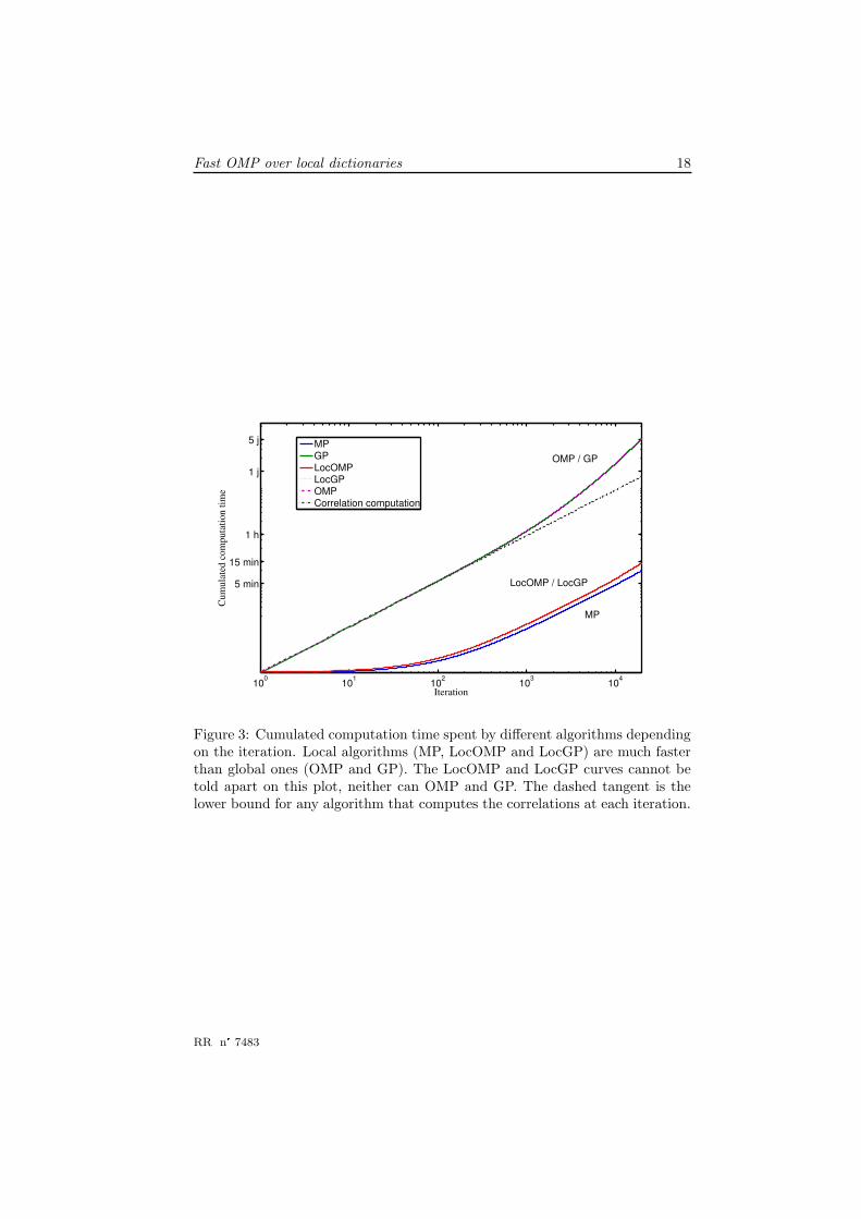
Figure 3 plots the cumulated computation time needed by each algorithm de-pending on the number of iterations. One can clearly see that OMP and GPare much slower than MP, LocGP and LocOMP. The figures had to be plottedin log− log scale so that all curves fit in the same plot.

It took about 5 days to global projection algorithms (OMP et GP) to com-plete the 20000 iterations whereas MP finished its run in only 10 minutes andboth LocOMP and LocGP only required about 15 minutes. This confirms nu-merically that LocOMP remains in the same order of cost as MP.

The slope of the curves towards the first iteration also provides interestinginsight. The curves of local algorithms start horizontally because the first it-eration is much more expensive than the other ones. So the cost to run oneiteration or a few ones is almost the same.

For global projection algorithms the slope towards the first iteration shows alinear behaviour in the log / log coordinates: at the beginning of the algorithm,OMP or GP have almost nothing else to do than recomputing the correlationsagain and again. When i grows, the projection step becomes more noticeableand the curves drift above their initial tangent. This tangent is a lower boundfor the cost of global projection algorithms: even if one could compute theprojection at no cost, a global algorithm could not cost less. This confirms theinterest of local updates.

6.3 Approximation quality

Figures 4 show the approximation quality defined as

SNR(i) = −10 log

∥

∥r(i)∥

∥

2

2

‖s‖22

(13)

depending on the iteration.The different curves are hard to distinguish on the original curve (left). Only

MP seems to provide significantly lower quality, all other curves are mixed.To get a closer look, we used OMP, that is presumably the best performing

algorithm under this experiment, as a reference. The right curve shows thedifference between the SNR achieved by OMP and the SNR achieved by eachalgorithm. One can see that the final loss of MP is equal to 0.6dB. LocOMPends up 0.01dB lower than OMP and LocGP 0.09dB lower. OMP and GPachieved the same quality on this experiment.

This confirms that the local update strategy, which only approximates OMP,can provide almost as good performance as the much more expensive, completeOMP, while remaining in the order of complexity of MP. The higher qualityloss of LocGP compared to LocOMP is still not explained. The algorithmic linkis the same between OMP and GP on one side and LocOMP and LocGP onthe other side. As OMP and GP share the same behaviour, one could expectLocOMP and LocGP to do the same.

RR n�7483


100 101 102 103 104

5 min

15 min

1 h

1 j

5 j

Iteration

Cum

ulat

ed c

ompu

tatio

n tim

e

MPGPLocOMPLocGPOMPCorrelation computation

MP

OMP / GP

LocOMP / LocGP

Figure 3: Cumulated computation time spent by different algorithms dependingon the iteration. Local algorithms (MP, LocOMP and LocGP) are much fasterthan global ones (OMP and GP). The LocOMP and LocGP curves cannot betold apart on this plot, neither can OMP and GP. The dashed tangent is thelower bound for any algorithm that computes the correlations at each iteration.

RR n�7483


0 0.5 1 1.5 2x 104

0

2

4

6

8

10

12

Iteration

SNR

(dB)

MPGPLocOMPLocGPOMP

MP

OMP / GP / LocOMP / LocGP

0 0.5 1 1.5 2x 104

−0.6

−0.4

−0.2

0

Iteration

SNR

loss

to O

MP

(dB)

MPGPLocOMPLocGPOMP

OMP / GP

LocGPLocOMP

MP

Figure 4: Approximation SNR obtained by several algorithms depending on theiteration. All the algorithms perform similarly apart from MP. The right plotshows the SNR loss compared to OMP.

On these experiments, the overall approximation quality of all algorithms,including OMP, is limited, with only 11dB reached after 20000 iterations. Thequality difference between MP and OMP is accordingly small. This is mainlydue to the choice of a small, short-scale dictionary. This choice was driven bythe will to provide a comparison with OMP, so the dictionary had to be smallenough so that we could actually afford to run OMP and GP.

More promising, although still preliminary, results are displayed in the nextsection with larger dictionaries. They show that LocGP provides a substantialquality gain over MP.

7 Theoretical study

LocOMP was designed to ensure that its complexity remains within that of MP,and its quality should lie somewhere between MP and OMP. In this section wediscuss which known theoretical guarantees that apply to both MP and OMPare also valid for LocOMP (resp. LocGP).

7.1 General MP, General Strong MP

The results presented in this section are based on the work of Tropp [12] andGribonval and Vandergheynst [13]. Tropp provided results for OMP, and Gri-bonval and Vandergheynst pointed out that some of these results are valid fora wider class of algorithms they labelled General MP. A General MP algorithmis an algorithm that at iteration i:

selects the atom with highest correlation to the residual,

computes an approximant that lies in the span of all previously computedatoms Φ(i).

One can easily see that LocOMP belongs to General MP.

RR n�7483


However, not all the results extend because the General MP class is toowide: it contains obviously non-functional algorithms such as selecting the bestatom then adding it (typos happen...) to the residual instead of subtracting it.In this paper we define a smaller class of algorithms that we call General StrongMP. This class intuitively corresponds to algorithms at least as good as MP. AGeneral Strong MP algorithm xMP is an algorithm that:

belongs to General MP;

ensures that from any given residual s, any dictionary Φ and after anynumber of xMP iterations i, one more iteration of xMP decreases theresidual energy at least as much as one iteration of MP.

Lemma 1. LocOMP and OMP belong to General Strong MP.

Proof. At iteration i, both MP, OMP and LocOMP update the residual with anorthogonal projection. MP projects the residual on the space SMP orthogonalto the last atom ϕ(i). OMP projects it on the space SOMP orthogonal tothe set of selected atoms Φ(i). LocOMP projects it on the space SLocOMP

orthogonal to the selected subdictionary Ψ(i). We conclude using the fact thatϕ(i) ∈ Ψ(i) ⊂ Φ(i) so SOMP ⊂ SLocOMP ⊂ SMP .

Lemma 2. GP and LocGP do not belong to General Strong MP.

Proof. One can build a counter-example where an iteration of MP would getan exact decomposition (yielding a zero residual), but not the correspondingiteration of GP. This example needs at least three iterations: GP and MP arealways identical over the first two iterations.

Consider the dictionary Φ made of the three atoms ϕ1 =(

1 0 0)

, ϕ2 =1√5

(

1 2 0)

and ϕ3 = 1√6

(

2 −1 1)

. Let s = 12ϕ1 + 2ϕ2

√5 − ϕ3

√6 =

(

12 5 −1)

. The first iteration of GP (or LocGP, since they share the same be-

haviour if the dictionary is not local) selects ϕ1 and leads to r(1) =(

0 5 −1)

.The second iteration selects ϕ2 and we let the reader check that GP leads tor(2) =

(

−2 1 −1)

= −ϕ3

√6. The third iteration selects ϕ3. An MP resid-

ual update would lead to r(3) = 0. However, the gradient is proportional toΦ∗r(2) = (−2, 0,−

√6) which is not in the direction of ϕ3 so GP leads to a

non-zero residual and does not decrease the energy of the residual as much as astep of MP would.

This observation is consistent with the convergence rate for GP proven byBlumensath and Davies [5], that is slower than MP in the worst case.

7.2 Recovery of exactly sparse vectors

Assume that the signal s is exactly k-sparse, i.e. there exists a K-sparse vectorxopt such that s = Φxopt. In that case, a natural question is whether thealgorithm can retrieve xopt. Let Φopt be the subdictionary of Φ associated to thenonzero entries of xopt. Tropp provided a sufficient Exact Recovery Condition(ERC) on the dictionary Φ for OMP to recover xopt [12]:

RR n�7483


Theorem 1 (Tropp). Denote Φopt = Φ \ Φopt and assume that

maxϕ∈ ¯Φopt

∥

∥Φ+optϕ

∥

∥

1< 1. (14)

Then, for any signal s = Φoptxopt, OMP recovers xopt in K = ‖xopt‖0 iterations.

Tropp only proves that under the ERC (14) OMP can only select atoms ofΦopt. The exact recovery comes form the fact that OMP can never select thesame atom twice, so if it keeps selecting optimal atoms it has to select themall. Gribonval and Vandergheynst pointed that the first part of the proof isalso valid for General MP. As LocOMP belongs to General MP, the followingtheorem holds:

Theorem 2 (Gribonval/Vandergheynst). With the same notations and assump-

tions as in Theorem 1, for any signal s = Φoptxopt, all the atoms selected by

LocOMP belong to Φopt.

7.3 Convergence speed for exactly sparse signals

There are also results for MP that guarantee a fix decay rate per iteration, thusan overall exponential decay. Indeed, if one can prove that for some 0 < η < 1,∥

∥r(i)∥

∥

2

2≤ η

∥

∥r(i−1)∥

∥

2

2, then

∥

∥r(i)∥

∥

2

2≤ ηi ‖s‖2

2.Mallat and Zhang proposed a geometrical bound [3] for η. In finite dimen-

sion, if the dictionary is complete, then there is a ρ > 0 such for any unitaryvector s, there at least one atom ϕ ∈ Φ such that | 〈s, ϕ〉 | ≥ ρ. Then, at iterationi, for any General Strong MP algorithm, we have

|⟨

r(i−1), ϕ(i)⟩

| ≥ ρ∥

∥

∥r(i−1)

∥

∥

∥

2∥

∥

∥r(i)∥

∥

∥

2

2≤∥

∥

∥r(i−1) −

⟨

r(i−1), ϕ(i)⟩

ϕ(i)∥

∥

∥

2

2

≤∥

∥

∥r(i−1)

∥

∥

∥

2

2−⟨

r(i−1), ϕ(i)⟩2

≤(

1 − ρ2)

∥

∥

∥r(i−1)

∥

∥

∥

2

2

so η = 1 − ρ2 is a lower bound for the decay rate. However this bound ispessimistic, especially in high dimension. For example, if the dictionary Φ isan orthonormal basis in dimension N , then the best possible ρ is 1√

Nand the

corresponding η is 1− 1N

, which tends towards 1 when the dimension N increases.Gribonval and Vandergheynst proposed another bound in the case of quasi-

incoherent dictionaries. The cumulative coherence µ1 of a dictionary Φ is afunction of K defined as

µ1(K) = maxϕ0∈Φ,(ϕk)1≤k≤K∈(Φ\{ϕ0})K

K∑

k=1

| 〈ϕ0, ϕk〉 | (15)

RR n�7483


This function measures how close to orthogonal the dictionary is: if it wasorthogonal, then µ1(K) would be 0 for any K ≤ N . If the cumulative coherenceincreases slowly with K, then the dictionary is called quasi-incoherent. In thatcase, the following theorem holds:

Theorem 3. Let Φ be a dictionary of cumulative coherence µ1. Let K be such

that µ1(K) + µ1(K − 1) < 1 and let Φopt ⊂ Φ be a sub-dictionary containing

K atoms. Then the ERC (14) holds for Φopt, and for any General Strong MP

algorithm, if s = Φoptxopt then

∀i > 0,∥

∥

∥r(i)∥

∥

∥

2

2≤(

1 − 1 − µ1(K − 1)

K

)i

‖s‖22 (16)

Proof. The reader can refer to the proof provided by Gribonval and Vandergheynstfor both MP and OMP. The proof for OMP only adds the fact that OMP de-creases the error more than MP on one iteration, so it is actually valid for thewhole General Strong MP class, including LocOMP.

7.4 Stable recovery of sparse vectors in the presence of

noise

Natural signals are usually not exactly sparse, either because the sparse model isonly a simplified approach or because the measurements were noisy. The signalmodel s = Φoptxopt + ε is therefore often more realistic than the exact sparsemodel s = Φoptxopt + ε. Tropp proved that with quasi-incoherent dictionaries,OMP manages to retrieve atoms belonging to Φopt until the residual error getssmall enough. Gribonval and Vandergheynst pointed that Tropp’s proof alsoholds for any General MP algorithm, including LocOMP and LocGP.

Theorem 4. Let Φ be a dictionary of cumulative coherence µ1. Let K be such

that µ1(K) + µ1(K − 1) < 1 and let Φopt ⊂ Φ be a sub-dictionary containing

K atoms. Let s = Φoptxopt + ε: LocOMP only selects atoms of Φopt until the

following error threshold is reached:

∥

∥

∥r(i)∥

∥

∥

2

2≤(

1 +K (1 − µ1(K − 1))

(1 − µ1(K − 1) − µ1(K))2

)

‖s − Φoptxopt‖22 (17)

7.5 Convergence speed in the presence of noise

Gribonval and Vandergheynst provided an upper bound for the number of iter-ations it takes MP to reach the error threshold of Theorem 4. This result canbe generalized to General Strong MP, hence LocOMP.

Theorem 5. With all the hypotheses of Theorem 4 still holding, let σ2K be the

residual energy of the best K-term approximant to s. If σ2K ≤ 3

σ21

K, then the

threshold of Theorem 4 is reached within at most

I = 2 +K

1 − µ1(K − 1)log

3σ21

Kσ2K

(18)

RR n�7483


iterations. If not, then the signal is too noisy to guarantee the recovery of atoms

from Φopt.

Proof. The reader can follow the proof by Gribonval and Vandergheynst. Theonly change needed to extend the proof to General Strong MP is in the proofof their Lemma 3. They use the fact that for MP,

∥

∥

∥r(i)∥

∥

∥

2

2−∥

∥

∥r(i+1)

∥

∥

∥

2

2=⟨

r(i), ϕ(i+1)⟩2

(19)

To extend the proof to General Strong MP, replace this equality with

∥

∥

∥r(i)∥

∥

∥

2

2−∥

∥

∥r(i+1)

∥

∥

∥

2

2≥⟨

r(i), ϕ(i+1)⟩2

(20)

8 Perspectives

8.1 MPTK implementation

An implementation of LocGP in the MPTK library is currently under develop-ment. A prototype is already running, but it is still much slower than expected.

We chose LocGP for software engineering reasons. MPTK currently does notuse any matrix computations thanks to fast dictionaries. We would like to keepit that way because it is programmed and C++ so the access to linear algebraslibraries is not native. The simple expression of the gradient in LocGP makesit possible to implement it without having to link MPTK with an externalmatrix library. As LocOMP seems to achieve significantly better quality, itsimplementation is also targeted in the long term.

Obtained quality We compared our prototype implementation of LocGPwith the MP implementation in MPTK. Only these two algorithms could becompared since C++ implementations of other algorithms were not available(and not worth developing) for OMP and GP. We still used 1 minute music sig-nals downsampled to 8 kHz but this time we used a multiscale MDCT dictionarywith scales L1 = 32 and L2 = 1024, which amount to 4ms and 128ms. Thesescales roughly correspond to the time windows used for AAC audio compression.Both algorithms were run for 20000 iterations.

Figure 5 shows the SNR depending on the iteration. We observe thatLocGP brings a average gain of 2dB over MP, which looks promising.

Computation time The obtained computation times are, however, disap-pointing. MP finished the whole computation in less than 10 minutes, whereasit almost took one day to run LocGP. Profiling of the LocGP program hints ata great time loss during residual update.

MPTK uses fast dictionaries. Correlations are computed using an FFT-based fast analysis algorithm. In MP, an atom that is selected at iteration

RR n�7483


0 0.2 0.4 0.6 0.8 1 1.2 1.4 1.6 1.8 2x 104

0

5

10

15

20

25

30

35

40

Iteration

SNR

(dB)

LocGPMP

Figure 5: Average approximation obtained by MP and LocGP depending on theiteration. The averages have been computed over 10 piano signals downsampledto 8 kHz. The decompositions used MDCT dictionaries with scale 32 and 1024.LocGP provides an average gain of 2dB over MP.

RR n�7483


i is only used at this iteration when it is removed from the residual, and alsomaybe if it is selected again later. Because of that the residual update has neverbeen a problem for MPTK and fast synthesis has not been implemented in theblocks. To subtract an atom from the residual, its waveform is synthesizedfrom its analytical definition and the subtraction is carried sample-wise. Onthe contrary, LocGP subtracts every atom of the sub-dictionary Ψ(i) at eachiteration. The synthesis of the waveforms over and over again seems to be thecause of the poor speed: LocGP spends its time computing cosines to generateoscillating waveforms. We are implementing a fast synthesis method to solve thisproblem. As the residual update is local, several atoms of the neighbourhoodΨ(i) should fall within the same few frames, which is what fast methods needto provide a gain over naive implementations.

8.2 Extension to multidimensional signals

LocOMP as described in this paper only applies to temporal series. However,local or shift-invariant dictionaries are also used in image processing. It wouldbe interesting to extend LocOMP to this case.

To do so, one needs to define the sub-dictionary Ψ(i). The notion of supportoverlapping is not specific to unidimensional signals: two atoms overlap if theyhave at least one atom in common. So the criteria to define Ψ(i) are still valid.

However Ψ(i) might be harder to extract from Φ(i). In the unidimensionalcase, the fast extraction is based on sorting the atoms (see C for more details).If the dimension of the signal grows, the location of the atoms is not providedby a single instant anymore but by a vector of coordinates. As the multi-dimensional coordinate spaces have no total ordering that preserveslocality, we will need to find another way to extract Ψ(i).

9 Conclusion

Sparse approximation over local dictionaries requires specific algorithms becauseof the large signal and dictionary dimensions that one wants to handle. MP wasalready known to be suitable for fast implementation over local dictionaries.

Contributions We proposed several algorithmic accelerations that enable afaster OMP implementation without changing the behaviour of the algorithm.All those accelerations still do not make OMP tractable because the correlationsλ = Φ∗r have to be computed at each iteration.

We proposed a new algorithm, LocOMP, whose behaviour is close to OMPfor a complexity that stays in the same class as MP. The key idea was to selecta sub-dictionary Ψ(i) containing only atoms located close to the last selectedatom ϕ(i). We also provided a fast way to extract Ψ(i) from Φ(i) by using asorted index of Φ(i).

LocOMP has shown experimentally that the approximations it computescan be as good as OMP.

RR n�7483


Perspectives We have proposed possible extensions of LocOMP, but for nowthe most urgent task to address is the optimization of the MPTK implemen-tation. Theoretical complexity and experimental results show that LocOMPfills the necessary speed and quality requirements to replace MP as a tractableapproximation algorithm, but it still lacks a high-performance implementationto reach its theoretical speed on real size data.

The link between the choice of Ψ(i) and the obtained quality has also yetto be fully understood. Larger sub-dictionaries lead to better approximations(on one iteration at least). Quantification of this evolution might help designbetter sub-dictionary selection heuristics as the one used here. This problem islinked to the theoretical study hinted at in Section 7, as both rely on theoreticalbounding of the approximation error. As we chose Ψ(i) as small as possible hereand still got almost as good results as OMP in this work, there might be noneed for larger sub-dictionaries.

Acknowledgements

The authors would like to thank the reviewers for their useful comments.

A Detailed explanations on the complexity of

greedy algorithms with general dictionaries

Hard Thresholding HT requires a matrix-vector product Φ∗s that is per-formed in O(DN), then the search for the K highest correlations is is lowerthan O(D log D) (which is the cost to sort them all), finally the amplitude com-putation can be performed in O(NK). As D > N � K, the main cost is thecost in O(DN) to compute the correlations.

MP One MP iteration is a thresholding with K = 1, so the correlation com-putation in O(DN) stays the most expensive part. The number of iterations torun to recover K different atoms is unknown. If one assumes that it stays inthe range of K, then the global algorithm cost is in O(DKN).

OMP OMP performs the same computations as MP, plus an orthogonal pro-jection, at each iteration. This projection consists in computing the Grammatrix G(i) = Φ(i)∗Φ(i), invert it and apply the inverse to a correlation vectorthat is already known from the selection step. Pati proposed a way to computethe new inverse G(i)−1 from the previous one G(i−1)−1 [4]. The main cost inO(iN) is spent computing the new line of the Gram matrix Φ(i−1)∗ϕ(i). Thenthe previous inverse has to be applied once, which is done in O(i2). This leadsto a total cost in O(K2N), that is no more than th cost to compute only theprojection on the final dictionary Φ(K)∗Φ(K).

RR n�7483


GP The gradient ∇x(i) is composed of correlations that are already knownfrom the selection step. The computation of ρ requires one more synthesis inO(D log N). Then one just have to change the coefficients, which is done inO(i). Compared to OMP, the cost in O(i2) has been decreased to O(i).

B Average proportion of overlapping atoms

When updating the Gram matrix, how many atoms are there Φ(i−1) that overlapϕ(i)? Let us assume that tmin(ϕ(i)) belongs to the interval J = [L−1, N−2L+1].Then

I = [tmin(ϕ(i)) − L + 1, tmin(ϕ(i)) + L − 1] (21)

and the length of I is 2L − 1. If the tmin of the other atoms of Φ(i−1)aresupposed independent and uniformly distributed over the interval [0, N − L],then the probability p for an atom to fall in the neighbourhood I is given by

p =2L − 1

N − L + 1(22)

and as there i− 1 atoms in Φ(i−1) the average number of selected atoms equals

(i − 1)p =(i − 1)(2L − 1)

N − L + 1= O

(

iL

N

)

(23)

C Data structures for fast access to selected atoms

Fast recovery of the connected component of ϕ(i) The atoms of Φ(i−1)

that overlap the last atom ϕ(i) can be found without traversing the whole sub-dictionary Φ(i−1) by maintaining a sorted index of the atoms. If atoms areordered with increasing tmin, then one just have to find the atoms with thesmallest and the largest admissible tmin and select every atom between thosetwo. Moreover the sorted index is dynamic as a new atom is added each itera-tion. So the index needs to be fast at:

inserting a new element,

extracting a sub-index between 2 given boundaries,

browsing that sub-index.

These criteria are fulfilled by sorted set implementation based on Red-Blacktrees, such as the ones used in the Java 3 and C++ 4 standard libraries. Theinsertion of tmin(ϕ(i)) is performed in O(log i) as well as the search for theboundaries, and the browsing of a sub-index containing Q elements is performedin O(Q). This leaves a global cost for the Gram matrix computation step equalto

O

(

log i +iL2

N

)

= O(

κ2iN)

(24)

3http://java.sun.com/javase/6/docs/api/java/util/TreeSet.html4http://gcc.gnu.org/onlinedocs/libstdc++/libstdc++-html-USERS-4.4/a00528.html

RR n�7483


Double indexing The Gram matrix G(i) = Φ(i)∗Φ(i) is a dynamic matrixthat grows by one line and column per iteration. To be able to store this matrixwithout having to move elements, one would like the new line and column tobe added at the end of the matrix. This means that two different indexes haveto be maintained for Φ(i): the increasing tmin index and the increasing i index.The first index is used to find the correlated atoms with ϕ(i) and the secondone to access coefficients in G(i).

C.1 MPTK implementation

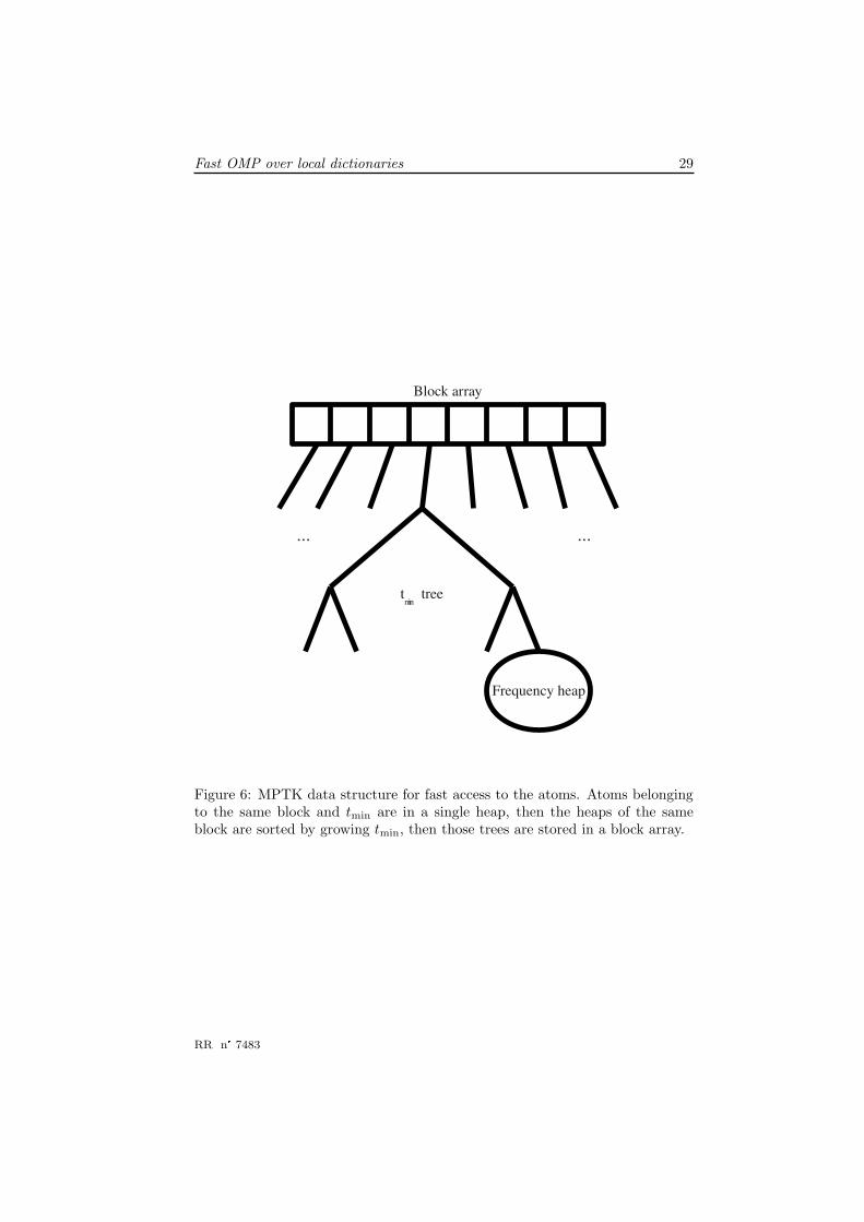
It has already been noted in Section C that the selection of Ψ(i) can be performedefficiently thanks to a sorted time index but that the order in which atoms areadded to the book must also be stored. MPTK implementation adds anotherconstraint to the indexing of selected atoms.

In MPTK, the dictionary is a collection of blocks. Each block is a filter bankthat implements fast analysis for a given family of atoms. For example, there isone block per scale when using a multiscale STFT dictionary.

LocGP needs to know the correlations Ψ(i)∗r(i−1) during the projection step.Theoretically, these have been computed in the previous selection step. How-ever, most of them are not stored in MPTK as they are not useful for MP. Sothe useful correlations have to be detected and saved during the selection stepbefore they are forgotten. This requires the extraction of all the atoms producedby a given block.

To do so we chose a hierarchical structure described in Figure 6. The atomsare first sorted according to their block, then their tmin, then other parameters(the frequency for STFT atoms).

This structure slows the extraction of Ψ(i) a little. If there are B blocks,then the extraction has to be performed B times for a total cost of O(B log i

B)

instead of O(log i). However the number of blocks is usually small. Browse andinsertion times do not change significantly.

D “Fast” exact OMP implementation for local

dictionaries

The shift-invariant structure could be used to provide a faster implementation ofOMP as it was done for MP in MPTK. We show that even with these improve-ments, OMP would remain much slower than MP. This will point which part ofthe algorithm is the most costly and worth replacing with a faster, suboptimalstep.

D.1 Correlation computation

As for MP, the cost of a fast analysis is reduced to O(D log L) but contrary toMP, the residual change r(i) − r(i−1) is global. As detailed in Algorithm 2, at

RR n�7483


Figure 6: MPTK data structure for fast access to the atoms. Atoms belongingto the same block and tmin are in a single heap, then the heaps of the sameblock are sorted by growing tmin, then those trees are stored in a block array.

RR n�7483


iteration i − 1 the coefficient update χ(i−1) = x(i−1) − x(i−2) is equal to

χ(i−1) =(

Φ(i−1)∗Φ(i−1))−1

Φ(i−1)∗r(i−2) (25)

Some of the χ(i−1) can be null. First, r(i−2) is orthogonal to Φ(i−2) soΦ(i−1)∗r(i−2) =

⟨

ϕ(i−1), r(i−2)⟩

δϕ,ϕ(i−1) . Then, if the Gram matrix has thefollowing block structure

Φ(i−1)∗Φ(i−1) =

(

A 00 B

)

(26)

then the inverse is equal to

(

Φ(i−1)∗Φ(i−1))−1

=

(

A−1 00 B−1

)

(27)

In this case, only the coefficients of χ(i−1) belonging to the block that containsthe last atom ϕ(i−1) can be non-zero. Let Γ be the undirected graph that hasthe atoms of Φ(i−1) as vertexes and a link between two atoms if their correlationis non-zero. Then the blocks of the Gram matrix are the connected componentsof Γ.

Local dictionaries are more likely to provide such a block structure for theGram matrix of the sub-dictionary Φ(i−1) (to a permutation): two atoms whosesupports do not overlap are not correlated. So if there is a time t in the signalthat is not inside the support of any atom of Φ(i−1), then all the atoms either endbefore t or start after t. So there are at least 2 distinct connected componentsin Γ, and the residual can only change over the time support of the componentthat contains the last atom ϕ(i).

But do such t always exist? If enough atoms are selected their supports cancover the whole support of s. Then Γ is connected and the residual changesover its whole support. This behaviour seems likely at the end of OMP.

D.2 Gram matrix computation

Principle The Gram matrix G(i) = Φ(i)∗Φ(i) can be computed faster if thedictionary is local. First, as atoms only have a support length L, a cross-correlation can be computed in O(L) instead of O(N). Second, less correlationsare required. As two atoms whose supports do not overlap are uncorrelated, theGram matrix is sparse and the position of its zero coefficients can be predicted.The prediction consists in a simple test on the support begin tmin and end tmax:

supp(ϕ) ∩ supp(ϕ(i)) 6= ∅ ⇔{

tmax(ϕ) ≥ tmin(ϕ(i))tmin(ϕ) ≤ tmax(ϕ

(i))(28)

⇔{

tmin(ϕ) + L − 1 ≥ tmin(ϕ(i))tmin(ϕ) ≤ tmin(ϕ(i)) + L − 1

(29)

⇔ tmin(ϕ(i)) − L < tmin(ϕ) < tmin(ϕ(i)) + L (30)

RR n�7483


So an atom ϕ overlaps the last atom ϕ(i) if tmin(ϕ) belongs to the interval

I = [max{tmin(ϕ(i)) − L + 1, 0},min{tmin(ϕ(i)) + L − 1, N − L}]

Naive implementation How to find the atoms of Φ(i−1) that overlap thelast atom ϕ(i)? The direct way would be to browse Φ(i−1) and to compute thescalar product for atoms that satisfy the constraint (30). It can be assumedthat there are O

(

iLN

)

atoms to be selected (see B for justification). Then thecost for this step would be

O(

|Φ(i−1)| + LE(i))

= O

(

(i − 1) +L(i − 1)(2L − 1)

N − L + 1

)

(31)

= O

(

i +iL2

N

)

(32)

This cost encompasses the O(i) cost of the traversal of Φ(i−1) and the com-putation time for selected atoms. One can see that the computation time has

been reduced by a factor(

LN

)2. The first L

Nfactor comes from the fastest com-

putation of one scalar product and the second from the smaller amount of scalarproducts to be computed. Yet, the traversal cost is not guaranteed to be smallerthan the effective computation time. In C we show that this cost can be avoidedby using a sorted data structure.

Fast dictionaries Correlations between atoms can also be computed usingFFT or other fast algorithms if the dictionary enables it. FFT decreases thecosts by computing the correlations with a basis of L atoms in a single step.For many fast local dictionaries such as Short Term Fourier Transform, localityis defined for a basis: all the atoms that are processed together by the FFTshare the same support. Those dictionaries can combine the fast correlationalgorithm and our fast detection of zero correlations for a cost in O(L log L):one only needs to compute correlations between ϕ(i) and the few bases thatoverlap it. This implementation is not always interesting: when computing theGram matrix one only needs the atoms that:

overlap ϕ(i)

belong to Φ(i−1)

The FFT will compute the correlations for a whole basis but because of thesecond criterion only some of them are useful. For the FFT to be faster thannaive scalar product computation, one needs

L log L <iL2

N(33)

i > Nlog L

L(34)

RR n�7483


Gram matrix inversion As seen before, the use of short, local atoms makesG(i) sparse. The number of atoms that overlap the last atom ϕ(i) given inEquation (23) is also the average number of non-zero coefficients on each line

of G(i). So there are totally about O(

i2LN

)

non-zero coefficients in G(i). This

is also the cost to invert G(i) using Pati’s method for example [4].So the total cost of an OMP iteration is reduced to

O

(

D log L +L log L

+

i2L

N

)

(35)

=O

(

N log L

(

α +L

N+

i2L

N2 log L

))

(36)

This cost is expressed using the FFT implementation to compute the Grammatrix. As we suppose L � N , the computation of the Gram matrix is muchfaster than the best atom selection. The Gram matrix inversion cost only be-comes relevant when

i & N

√

α log L

L(37)

Choosing for example N ≈ 106, α = 2 and L = 1024, the inversion cost wouldbecome relevant i & 140000, which does not seem highly sparse. So the mainterm in this complexity is due to the best atom selection in O(D log L), althoughthe Gram matrix inversion might become more expensive for large iterations.

D.2.1 Conclusion

In the general case, the best atom selection step is the same for MP and OMP.The only difference is the projection step. Working with local dictionaries de-creases the projection step for OMP and the selection step for MP. This stillleaves a speed gap between MP and OMP, but the speed difference betweenMP and OMP is mostly due to the selection step.

This invalidates previous attempts at fast approximate OMP such as GP.Those approaches tried to decrease the cost of the projection step, but in ourcase it is not the most expensive one. We need an algorithm that can decreasethe cost of the best atom selection compared to OMP. This is what LocOMPdoes.

RR n�7483


E Notations

Vectors ϕ atoms signalr residualx decomposition coefficientsλ correlations

Matrices Φ dictionaryΨ sub-dictionaryG Gram matrix

Indexing Xi ith column of matrix Xxi ith coefficient of vector x

x(i) variable x at iteration iDimensions N signal length

D number of atoms in the dictionaryK sparsity levelL atom support lengthT residual change support lengthI total number of iterationsα redundancy factor

Norms ‖r‖2 euclidean norm‖x‖0 number of non-zero coefficients in x

Misc. 〈ϕ1, ϕ2〉 scalar productargminE f(e) element e of E that minimizes f(e)

M∗ adjoint of M

References

[1] S. Krstulovic, R. Gribonval, MPTK: Matching Pursuit made tractable,in: Proc. Int. Conf. Acoust. Speech Signal Process. (ICASSP’06), Vol. 3,Toulouse, France, 2006, pp. 496–499. doi:10.1109/ICASSP.2006.1660699.URL http://www.irisa.fr/metiss/gribonval/Conf/2006/ICASSP06%

/2006_ICASSP_KrstulovicGribonval_MPTK.pdf

[2] G. Davis, S. Mallat, M. Avellaneda, Adaptive greedy approximations, Con-str. Approx. 13 (1) (1997) 57–98.

[3] S. Mallat, Z. Zhang, Matching pursuits with time-frequency dictionar-ies, Signal Processing, IEEE Transactions on 41 (12) (1993) 3397–3415.doi:10.1109/78.258082.

[4] Y. C. Pati, R. Rezaiifar, Y. C. P. R. Rezaiifar, P. S. Krishnaprasad, Orthog-onal matching pursuit: Recursive function approximation with applicationsto wavelet decomposition, in: Proceedings of the 27 th Annual AsilomarConference on Signals, Systems, and Computers, 1993, pp. 40–44.

RR n�7483


[5] T. Blumensath, M. Davies, In greedy pursuit of new directions: (nearly)orthogonal matching pursuit by directional optimisation, in: Proc. EU-SIPCO’08, 2008.

[6] D. Needell, J. Tropp, Cosamp: Iterative signal recovery from incompleteand inaccurate samples, Applied and Computational Harmonic Analysis.

[7] W. Dai, O. Milenkovic, Subspace pursuit for compressive sensing signalreconstruction, Information Theory, IEEE Transactions on 55 (5) (2009)2230 –2249. doi:10.1109/TIT.2009.2016006.

[8] T. Blumensath, M. E. Davies, Normalised iterative hard thresholding; guar-anteed stability and performance, Tech. rep. (feb 2009).

[9] T. Blumensath, M. Davies, Iterative hard thresholding for compressed sens-ing, Applied and Computational Harmonic Analysis.

[10] R. Garg, R. Khandekar, Gradient descent with sparsification: an it-erative algorithm for sparse recovery with restricted isometry property,in: ICML ’09: Proceedings of the 26th Annual International Conferenceon Machine Learning, ACM, New York, NY, USA, 2009, pp. 337–344.doi:http://doi.acm.org/10.1145/1553374.1553417.

[11] G. Masataka, Development of the rwc music database, in: Proceedings ofthe 18th International Congress on Acoustics (ICA 2004), 2004, pp. I–553–556.

[12] J. Tropp, Greed is good: algorithmic results for sparse approximation,IEEE Transactions on Information Theory.

[13] R. Gribonval, P. Vandergheynst, On the exponential convergence of match-ing pursuits in quasi-incoherent dictionaries, Information Theory, IEEETransactions on 52 (1) (2006) 255–261.

RR n�7483

Centre de recherche INRIA Rennes – Bretagne AtlantiqueIRISA, Campus universitaire de Beaulieu - 35042 Rennes Cedex (France)

Centre de recherche INRIA Bordeaux – Sud Ouest : Domaine Universitaire - 351, cours de la Libération - 33405 Talence CedexCentre de recherche INRIA Grenoble – Rhône-Alpes : 655, avenue de l’Europe - 38334 Montbonnot Saint-Ismier

Centre de recherche INRIA Lille – Nord Europe : Parc Scientifique de la Haute Borne - 40, avenue Halley - 59650 Villeneuve d’AscqCentre de recherche INRIA Nancy – Grand Est : LORIA, Technopôle de Nancy-Brabois - Campus scientifique

615, rue du Jardin Botanique - BP 101 - 54602 Villers-lès-Nancy CedexCentre de recherche INRIA Paris – Rocquencourt : Domaine de Voluceau - Rocquencourt - BP 105 - 78153 Le Chesnay Cedex

Centre de recherche INRIA Saclay – Île-de-France : Parc Orsay Université - ZAC des Vignes : 4, rue Jacques Monod - 91893 Orsay CedexCentre de recherche INRIA Sophia Antipolis – Méditerranée : 2004, route des Lucioles - BP 93 - 06902 Sophia Antipolis Cedex

ÉditeurINRIA - Domaine de Voluceau - Rocquencourt, BP 105 - 78153 Le Chesnay Cedex (France)��

ISSN 0249-6399

fast orthogonal sparse approximation algorithms over local … · fast orthogonal sparse...

Documents