sabmis: sparse approximation based blind multi-image
TRANSCRIPT

arX
iv:2
110.
1141
8v1
[cs
.CR
] 2
1 O
ct 2
021
SABMIS: Sparse Approximation based
Blind Multi-Image Steganography Scheme
Rohit Agrawal1, Kapil Ahuja1, Marc C. Steinbach2, and Thomas Wick2
1Computer Science and Engineering, Indian Institute of Technology Indore, India2Leibniz Universitat Hannover, Institut fur Angewandte Mathematik, Hannover, Germany
Corresponding author:
Kapil Ahuja
Email address: [email protected]
ABSTRACT
Steganography is a technique of hiding secret data in some unsuspected cover media
so that it is visually imperceptible. The secret data as well as the cover media may be
text or multimedia. Image steganography, where the cover media is an image, is one
of the most commonly used schemes. Here, we focus on image steganography where
the hidden data is also an image. Specifically, we embed grayscale secret images
into a grayscale cover image, which is considered to be a challenging problem. Our
goal is to develop a steganography scheme with enhanced embedding capacity while
preserving the visual quality of the stego-image and ensuring that the stego-image is
resistant to steganographic attacks.
Our proposed scheme involves use of sparse approximation and our novel embed-
ding rule, which helps to increase the embedding capacity and adds a layer of se-
curity. The stego-image is constructed by using the Alternating Direction Method of
Multipliers (ADMM) to solve the Least Absolute Shrinkage and Selection Operator
(LASSO) formulation of the underlying minimization problem. This method has a fast
convergence, is easy to implement, and also is extensively used in image processing.
Finally, the secret images are extracted from the constructed stego-image using the
reverse of our embedding rule. Using these components together helps us to embed
up to four secret images into one cover image (instead of the common embedding
of two secret images) and forms our most novel contribution. We term our scheme
SABMIS (Sparse Approximation Blind Multi-Image Steganography).
We perform extensive experiments on several standard images, and evaluate the
embedding capacity, Peak Signal-to-Noise Ratio (PSNR) value, mean Structural Sim-
ilarity (MSSIM) index, Normalized Cross-Correlation (NCC) coefficients, entropy, and
Normalized Absolute Error (NAE). We obtain embedding capacities of 2 bpp (bits per
pixel), 4 bpp, 6 bpp, and 8 bpp while embedding one, two, three, and four secret im-
ages, respectively. These embedding capacities are higher than all the embedding
capacities obtained in the literature until now. Further, there is very little deteriora-
tion in the quality of the stego-image as compared to its corresponding cover image
(measured by above metrics). The quality of the original secret images and their
corresponding extracted secret images is also almost the same. Further, due to our
algorithmic design, our scheme is resistant to steganographic attacks as well.

1 INTRODUCTION
The primary concern during the transmission of digital data over communication media
is that anybody can access this data. Hence, to protect the data from being accessed by
illegitimate users, the sender must employ some security mechanisms. In general, there
are two main approaches used to protect secret data; cryptography (Stallings, 2019) and
steganography (Kordov and Zhelezov, 2021), with our focus on the latter.
Steganography is derived from the Greek words steganos for “covered” or “secret”
and graphie for “writing”. In steganography, the secret data is hidden in some unsus-
pected cover media so that it is visually imperceptible. Here, both the secret data as
well as the cover media may be text or multimedia. Recently, steganography schemes
that use images as secret data as well as cover media have gained a lot of research in-
terest due to their heavy use in World Wide Web applications. This is the focus of our
work.
Next, we present some relevant previous studies in this domain. Secret data can
be embedded in images in two ways; spatially or by using a transform. In the spatial
domain based image steganography scheme, secret data is embedded directly into the
image by some modification in the values of the image pixels. Some of the past works
related to this are given in Table 1. In the transform domain based image steganography
scheme, first, the image is transformed into frequency components, and then the secret
data is embedded into these components. Some of the past works related to this are
given in Table 2.
Table 1. Spatial domain-based image steganography schemes.
Reference Technique Secret images Cover image
(Baluja, 2019)
A modified version of
Least Significant Bits
(LSB) with deep
neural networks
2 color color
(Gutub and Shaarani, 2020) LSB 2 color color
(Guttikonda et al., 2018) LSB 3 binary grayscale and color
Images are of three kinds; binary, grayscale, and color. A grayscale image has more
information than a binary image. Similarly, a color image has more information than
a grayscale image. Thus, hiding a color secret image is more challenging than hiding
a grayscale secret image, which is more challenging than hiding a binary secret image.
Similarly, applying this concept to the cover image, we see a reverse sequence; see
Table 3. We focus on the middle case here, i.e., when both the secret images and the
cover image are grayscale, which is considered challenging.
The difficulty in designing a good steganography scheme for embedding secret im-
ages into a cover image is increasing the embedding capacity of the scheme while
preserving the quality of the resultant stego-image as well as making the scheme re-
sistant to steganographic attacks. Usually, the more the number of secret images to
be embedded (which often translates to heavier secret images), the lower the quality
of the obtained stego-image. Hence, we need to balance these two competing require-
ments. Until now, in most works, researchers have embedded two secret images in a
cover image. Some people have looked at embedding three secret images but this is
ii/xxiv

Table 2. Transform domain-based image steganography schemes.
Reference Technique Secret images Cover image
(Sanjutha, 2018)
Discrete Wavelet
Transformation (DWT)
with Particle Swarm
Optimization (PSO)
1 grayscale color
(Arunkumar et al., 2019a)
Redundant Integer Wavelet
Transform (RIWT) and QR
factorization
1 binary color
(Maheswari and Hemanth, 2017)
Contourlet and Fresnelet
Transformations with
Genetic Algorithm (GA)
and PSO
1 binary
(specifically, QR code)grayscale
(Arunkumar et al., 2019b)
RIWT, Singular Value
Decomposition (SVD),
and Discrete Cosine
Transformation (DCT)
1 binary grayscale
(Hemalatha et al., 2013) DWT 2 grayscale color
(Gutub and Shaarani, 2020) DWT and SVD 2 color color
rare (Guttikonda et al., 2018). Here, not just the number of secret images but the total
size of the secret images is also important. To capture this requirement of number as
well as size, a metric of bits per pixel (bpp) is used.
In this work, we present a novel image steganography scheme wherein up to four
images can be hidden in a single cover image. The size of a secret image is about
half of that of the cover image, which results in a very high bpp capacity. No one has
attempted embedding up to four secret images in a cover image until now, and those
who have attempted embedding one, two, or three images have also not achieved the
level of embedding capacity that we do. While enhancing the capacity as discussed
above, the quality of our stego-image does not deteriorate much. Also, we do not need
any cover image data to extract secret images on the receiver side, which is commonly
required with other schemes. We do require some algorithmic settings on the receiver
side, however, these can be communicated to the receiver separately. Thus, this makes
our scheme more secure.
Our innovative scheme has three components, which we discuss next. The first
component, i.e., embedding of secret images, consists of the following parts:
(i) We perform sub-sampling on a cover image to obtain four sub-images of the cover
image.
(ii) We perform block-wise sparsification of each of these four sub-images using DCT
(Discrete Cosine Transform) and form a vector.
(iii) We represent each vector in two groups based upon large and small coefficients,
and then project each of the resultant (or generated) sparse vector onto linear measure-
ments by using a measurement matrix (random matrix whose columns are normalized).
The oversampling at this stage leads to sparse approximation.
(iv) We repeat the second step above for each of the secret images.
(v) We embed DCT coefficients from the four secret images into “a set” of linear mea-
surements obtained from the four sub-images of the cover image using our new embed-
iii/xxiv

Table 3. Image types and levels of challenge.
Image Type More Challenging Medium Challenging Less Challenging
Secret Image Color Grayscale Binary
Cover Image Binary Grayscale Color
ding rule.
Second, we generate the stego-image from these modified measurements by using
the Alternating Direction Method of Multipliers (ADMM) to solve the Least Absolute
Shrinkage and Selection Operator (LASSO) formulation of the underlying minimiza-
tion problem. This method has fast convergence, is easy to implement, and also is ex-
tensively used in image processing. Here, the optimization problem is an ℓ1-norm mini-
mization problem, and the constraints comprise an over-determined system of equations
(Srinivas and Naidu, 2015).
Third, we extract the secret images from the stego-image using our proposed ex-
traction rule, which is the reverse of our embedding rule mentioned above. As men-
tioned earlier, we do not require any information about the cover image while doing
this extraction, which makes the process blind. We call our scheme SABMIS (Sparse
Approximation Blind Multi-Image Steganography).
For performance evaluation, we perform extensive experiments on a set of standard
images. We first compute the embedding capacity of our scheme, which turns out to
be very good. Next, we check the quality of the stego-images by comparing them with
their corresponding cover images. We use both a visual measure and a set of numerical
measures for this comparison. The numerical measures used are: Peak Signal-to-Noise
Ratio (PSNR) value, Mean Structural Similarity (MSSIM) index, Normalized Cross-
Correlation (NCC) coefficient, entropy, and Normalized Absolute Error (NAE). The
results show very little deterioration in the quality of the stego-images.
Further, we visually demonstrate the high quality of the extracted secret images
by comparing them with the corresponding original secret images. Also, via experi-
ments, we support our conjecture that our scheme is resistant to steganographic attacks.
Finally, we compare the embedding capacity of our scheme and PSNR values of our
stego-images with the corresponding data from competitive schemes available in the
literature1. These last two checks (quality of the extracted secret images and experi-
mentation for resistance to steganographic attacks) are not common in existing works,
and hence, we are unable to perform these two comparisons. The superiority of our
scheme over past works is summarized below.
Because of the lack of past work of embedding grayscale secret images into a
grayscale cover image, we compare with the cases of embedding binary images into
a grayscale image or embedding grayscale images into a color image. Both these prob-
lems are easier than our problem as discussed earlier; see Table 3.
For the case of embedding one secret image into a cover image, we compare with
(Arunkumar et al., 2019b). Here, a binary secret image is embedded into a grayscale
1Most of the existing works do not compute the other numerical mesaures of SSIM index, NCC
coefficient, entropy and NAE.
iv/xxiv

cover image. The authors in (Arunkumar et al., 2019b) achieve an embedding capacity
of 0.25 bpp while we achieve an embedding capacity of 2 bpp. When comparing the
stego-image and the corresponding cover image, (Arunkumar et al., 2019b) achieve a
PSNR value of 49.69 dB while we achieve a PSNR value of 43.15 dB. This is consid-
ered acceptable because we are compromising very little in quality while gaining a lot
more in embedding capacity. Moreover, PSNR values over 30 dB are considered good
(Gutub and Shaarani, 2020; Zhang et al., 2013; Liu and Liao, 2008).
For the case of embedding two secret images in a cover image, we compare with
(Hemalatha et al., 2013). Here, two grayscale images are embedded into a color cover
image. The authors in (Hemalatha et al., 2013) achieve an embedding capacity of
1.33 bpp while we achieve an embedding capacity of 4 bpp. When comparing the stego-
image and the corresponding cover image, (Hemalatha et al., 2013) achieve a PSNR
value of 44.75 dB while we achieve a PSNR value of 39.83 dB. This is again consid-
ered acceptable because of the reason discussed above.
For the case of embedding three secret images in a cover image, we compare with
(Guttikonda et al., 2018). Here, three binary images are embedded into a grayscale
cover image. The authors in (Guttikonda et al., 2018) achieve an embedding capacity
of 2 bpp while we achieve an embedding capacity of 6 bpp. When comparing the stego-
image and the corresponding cover image, (Guttikonda et al., 2018) achieve a PSNR
value of 46.36 dB while we achieve a PSNR value of 38.12 dB. Again, this is considered
acceptable.
When embedding four secret images in a cover image, we achieve an embedding
capacity of 8 bpp and a PSNR value of 37.14 dB, which no one else has done.
The remainder of this paper has three more sections. In Section 2, we present
our proposed sparse approximation based blind multi-image steganography scheme.
The experimental results are presented in Section 3. Finally, in Section 4, we discuss
conclusions and future work.
2 PROPOSED APPROACH
Our sparse approximation based blind multi-image steganography scheme consists of
the following components: (i) Embedding of secret images leading to the generation of
the stego-data. (ii) Construction of the stego-image. (iii) Extraction of secret images
from the stego-image. These parts are discussed in the respective subsections below.
2.1 Embedding Secret Images
First, we perform sub-sampling of the cover image to obtain four sub-images. This type
of sampling is done because we are embedding up to four secret images. Let CI be the
cover image of size r× r. Then, the four sub-images each of size r2× r
2are obtained as
follows (Pan et al., 2015):
CI1(n1,n2) =CI(2n1−1,2n2 −1), (1a)
CI2(n1,n2) =CI(2n1,2n2 −1), (1b)
CI3(n1,n2) =CI(2n1−1,2n2), (1c)
CI4(n1,n2) =CI(2n1,2n2), (1d)
v/xxiv
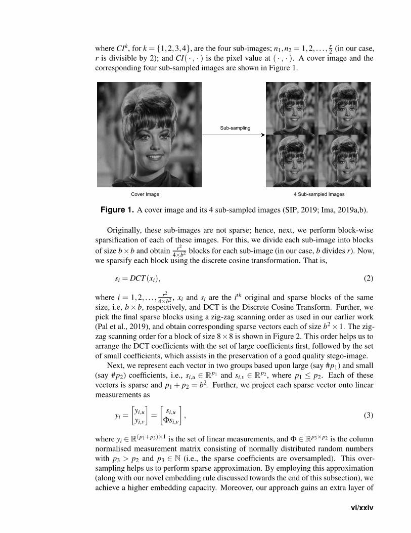
where CIk, for k = {1,2,3,4}, are the four sub-images; n1,n2 = 1,2, . . . , r2
(in our case,
r is divisible by 2); and CI( · , · ) is the pixel value at ( · , · ). A cover image and the
corresponding four sub-sampled images are shown in Figure 1.
Cover Image
Sub-sampling
4 Sub-sampled Images
Figure 1. A cover image and its 4 sub-sampled images (SIP, 2019; Ima, 2019a,b).
Originally, these sub-images are not sparse; hence, next, we perform block-wise
sparsification of each of these images. For this, we divide each sub-image into blocks
of size b×b and obtain r2
4×b2 blocks for each sub-image (in our case, b divides r). Now,
we sparsify each block using the discrete cosine transformation. That is,
si = DCT (xi), (2)
where i = 1,2, . . . , r2
4×b2 , xi and si are the ith original and sparse blocks of the same
size, i.e, b× b, respectively, and DCT is the Discrete Cosine Transform. Further, we
pick the final sparse blocks using a zig-zag scanning order as used in our earlier work
(Pal et al., 2019), and obtain corresponding sparse vectors each of size b2 ×1. The zig-
zag scanning order for a block of size 8×8 is shown in Figure 2. This order helps us to
arrange the DCT coefficients with the set of large coefficients first, followed by the set
of small coefficients, which assists in the preservation of a good quality stego-image.
Next, we represent each vector in two groups based upon large (say #p1) and small
(say #p2) coefficients, i.e., si,u ∈ Rp1 and si,v ∈ R
p2 , where p1 ≤ p2. Each of these
vectors is sparse and p1 + p2 = b2. Further, we project each sparse vector onto linear
measurements as
yi =
[
yi,u
yi,v
]
=
[
si,u
Φsi,v
]
, (3)
where yi ∈R(p1+p3)×1 is the set of linear measurements, and Φ ∈R
p3×p2 is the column
normalised measurement matrix consisting of normally distributed random numbers
with p3 > p2 and p3 ∈ N (i.e., the sparse coefficients are oversampled). This over-
sampling helps us to perform sparse approximation. By employing this approximation
(along with our novel embedding rule discussed towards the end of this subsection), we
achieve a higher embedding capacity. Moreover, our approach gains an extra layer of
vi/xxiv

security because the linear measurements are measurement-matrix encoded small coef-
ficients of the sparse vectors obtained after DCT. Since the distribution of coefficients
of the generated sparse vectors is almost the same for all the blocks of an image, we
use the same measurement matrix for all the blocks.
Figure 2. Zig-zag scanning order for a block of size 8×8.
Next, we perform processing of the secret images for embedding them into the
cover image. Let the size of each secret image be m×m. Initially, we perform block-
wise DCT of each of these images and obtain their corresponding DCT coefficients.
Here, the size of each block taken is l× l, and hence, we have m2
l2 blocks for each secret
image. In our case, l divides m, and we ensure that m2
l2 will be less than or equal to r2
4×b2
so that the number of blocks of the secret image is less than or equal to the number of
blocks of a sub-image. Thereafter, we arrange these DCT coefficients as a vector in
the earlier discussed zig-zag scanning order. Let tı ∈ Rl2×1, for ı = 1,2, . . . , m2
l2 , be the
vector representation of the DCT coefficients of one secret image. We pick the initial
p4 DCT coefficients with relatively larger values (out of the available l2 coefficients)
for embedding, where p4 ∈ N.
Here, we show the embedding of only one secret image into one sub-image of the
cover image. However, in our steganography scheme, we can embed a maximum of
four secret images, one in each of the four sub-images of the cover image, which is
demonstrated in the experimental results section. If we want to embed less than four
secret images, we can randomly select the corresponding sub-images from the available
four.
Next, using our novel embedding rule (discussed below), we embed the chosen p4
DCT coefficients of the secret image into a selected set of p1+ p3 linear measurements
obtained from the sub-image of the cover image, leading to the generation of the stego-
data (we ensure that p4 is less than p1 + p3). The selected linear measurements are
chosen to give the best results, i.e., satisfy all the three goals of higher embedding
capacity, less deterioration in the quality of the stego-image and more security.
Initially, we embed the first coefficient of the secret image into the (p1−2c)th index
vii/xxiv

of the original linear measurements vector to obtain the pth1 index of the resultant mod-
ified linear measurements vector (where c is some user chosen constant). Further, we
embed the next c−1 coefficients from the secret image into p1 −2c+1 to p1 − c−1
indices of the original linear measurements vector to obtain the p1 − c+ 1 to p1 − 1
indices of the resultant modified linear measurements vector.
Finally, we embed the remaining p4−c coefficients from the secret image into p1+c+1 to p1+ p4 indices of the original linear measurements vector to obtain p1+ p4+1
to p1 + 2× p4 − c indices of the resultant modified linear measurements vector. The
whole process in given in Algorithm 1. Specifically, the embedding rules discussed
above are given on line 3, lines 4 – 6, and lines 7 – 9 of this algorithm, respectively.
2.2 Construction of the Stego-Image
As mentioned earlier, the next step in our scheme is the construction of the stego-image.
Since we can embed a maximum of four secret images into four sub-images of a single
cover image, we first construct four sub-stego-images and then perform inverse sam-
pling to obtain a single stego-image. Let s′i be the sparse vector of the ith block of a
sub-stego-image. The sparse vector s′i is the concatenation of s′i,u and s′i,v. Here, the size
of s′i,u, s′i,v, and s′ is the same as that of si,u, si,v, and s, respectively. Then, we have
s′i,u = y′i,u, (4a)
s′i,v = argmins′i,v∈R
p2
‖s′i,v‖1 subject to Φs′i,v = y′i,v. (4b)
The second part (4b) (i.e., obtaining s′i,v), is an ℓ1-norm minimization problem. Here,
we can observe that in the above optimization problem, the constraints are oversam-
pled. As earlier, this oversampling helps us to do sparsification, which leads to in-
creased embedding capacity without degradation of the quality of both the stego-image
and the secret image. For the solution of the minimization problem (4b), we use
ADMM (Boyd et al., 2010; Gabay, 1976) to solve the LASSO (Hwang et al., 2016;
Nardone et al., 2019) formulation of this minimization problem. The reason is that this
method has a fast convergence, is easy to implement, and also is extensively used in
image processing (Boyd et al., 2010; Hwang et al., 2016).
Next, we convert each vector s′i into a block of size b× b. After that, we perform
inverse sparsification (i.e., we apply the two-dimensional Inverse DCT) to each of these
blocks to generate blocks x′i of the image. That is,
x′i = IDCT(
s′i)
. (5)
Next, we construct the sub-stego-image of size r2× r
2by arranging all these blocks x′i.
We repeat the above steps to construct all four sub-stego-images. At last, we perform
inverse sampling and obtain a single constructed stego-image from these four sub-stego-
images. In the experiments section, we show that the quality of the stego-image is also
very good.
2.3 Extraction of the Secret Images
In this subsection, we discuss the process of extracting secret images from the stego-
image. Initially, we perform sampling (as done in Section 2.1 using (1a)–(1d)) of the
viii/xxiv

Algorithm 1 Embedding Rule
Input:
• yi: Sequence of linear measurements of the cover image with i =
1,2, . . . , r2
4×b2 .
• tı: Sequence of transform coefficients of the secret image with ı =
1,2, . . . , m2
l2 .
• The choice of our r, b, m, and l is such that m2
l2 is less than or equal to r2
4×b2 .
• p1 and p4 are lengths of certain vectors defined on pages vi and vii, respec-
tively.
• α , β , γ , and c are algorithmic constants that are chosen based upon experi-
ence. The choices of these constants are discussed in the experimental results
sections.
Output:
• y′i: The modified version of the linear measurements with i = 1,2, . . . , r2
4×b2 .
1: Initialize y′i to yi, where i = 1,2, . . . , r2
4×b2 .
2: for i = 1 to r2
4×b2 do
3: // Embedding of the first coefficient.
y′i(p1) = yi(p1 −2c)+α × ti(1).
4: for j = p1 − c+1 to p1 −1 do
5: // Embedding of the next c−1 coefficients.
y′i( j) = yi( j− c)+β × ti( j− p1 + c+1).
6: end for
7: for k = p1 + p4 +1 to p1 +2× p4 − c do
8: // Embedding of the remaining p4 − c coefficients.
y′i(k) = yi(k− p4 + c)+ γ × ti(k− p1 − p4 + c).
9: end for
10: end for
11: return y′i
stego-image to obtain four sub-stego-images. Since the extraction of all the secret
images is similar, here, we discuss the extraction of only one secret image from one
sub-stego-image. First, we perform block-wise sparsification of the chosen sub-stego-
image. For this, we divide the sub-stego-image into blocks of size b× b. We obtain
a total of r2
4×b2 blocks. Further, we sparsify each block (say x′′i ) by computing the
corresponding sparse vector (say s′′i ). That is,
s′′i = DCT (x′′i ). (6)
ix/xxiv

Next, as earlier, we arrange these sparse blocks in a zig-zag scanning order, obtain
the corresponding sparse vectors each of size b2 ×1, and then categorize each of them
into two groups s′′i,u ∈Rp1 and s′′i,v ∈R
p2 . Here, as before, p1 and p2 are the numbers of
coefficients having large values and small values (or zero values), respectively. After
that, we project each sparse vector onto linear measurements (say y′′i ∈ R(p1+p3)×1),
y′′i =
[
y′′i,uy′′i,v
]
=
[
s′′i,uΦs′′i,v
]
. (7)
From y′′i , we extract the DCT coefficients of the embedded secret image using Algo-
rithm 2. This extraction rule is the reverse of the embedding rule given in Algorithm
1.
In Algorithm 2, t ′ı ∈Rl2×1, for ı = 1,2, . . . , m2
l2 , are the vector representations of the
DCT coefficients of the blocks of one extracted secret image. Next, we convert each
vector t ′ı into blocks of size l × l, and then perform a block-wise Inverse DCT (IDCT)
(using (5)) to obtain the secret image pixels. Finally, we obtain the extracted secret
image of size m×m by arranging all these blocks column wise. As mentioned earlier,
this steganography scheme is a blind multi-image steganography scheme because it
does not require any cover image data at the receiver side for the extraction of secret
images.
Here, the process of hiding (and extracting) secret images is not fully lossless2, re-
sulting in the degradation of the quality of extracted secret images. This is because we
first oversample the original image using (3), and then we construct the stego-image
by solving the optimization problem (4b), which leads to a loss of information. How-
ever, our algorithm is designed in such a way that we are able to extract high-quality
secret images. We support this fact with examples in the experiments section (specifi-
cally, Section 3.3). We term our algorithm Sparse Approximation Blind Multi-Image
Steganography (SABMIS) scheme due to the involved sparse approximation and the
blind multi-image steganography.
3 EXPERIMENTAL RESULTS
Experiments are carried out in MATLAB on a machine with an Intel Core i3 processor
@2.30 GHz and 4GB RAM. We use a set of 31 standard grayscale images available
from miscellaneous categories of the USC-SIPI image database (SIP, 2019) and two
other public domain databases (Ima, 2019a,b). In this work, we report results for 10
images (shown in Figure 3). However, our SABMIS scheme is applicable to other
images as well. Our selection is justified by the fact that the image processing literature
has frequently used these 10 images or a subset of them.
Here, we take all ten images shown in Figure 3 as the cover images, and four images;
Figures 3a, 3b, 3e and 3j as the secret images for our experiments. However, we can
use any of the ten images as the secret images.
Although the images shown in Figure 3 look to be of the same dimension, they are
of varying sizes. For our experiments, each cover image is converted to 1024× 1024
size (i.e., r× r). We take blocks of size 8×8 for the cover images (i.e., b×b). Recall
2This is common in transform-based image steganography.
x/xxiv

Algorithm 2 Extraction Rule
Input:
• y′′i : Sequence of linear measurements of the stego-image with i =
1,2, . . . , r2
4×b2 .
• p1 and p4 are lengths of certain vectors defined on pages vi and vii, respec-
tively.
• α , β , γ , and c are algorithmic constants that are chosen based upon experi-
ence. The choices of these constants are discussed in the experimental results
section.
Output:
• t ′ı : Sequence of transform coefficients of the secret image with ı =
1,2, . . . , m2
l2 .
1: Initialize t ′ı to zeros, where ı = 1,2, . . . , m2
l2 .
2: for i = 1 to r2
4×b2 do
3: // Extraction of the first coefficient.
t ′i(1) =y′′i (p1)−y′′i (p1−2c)
α .
4: for j = p1 − c+1 to p1 −1 do
5: // Extraction of the next c−1 coefficients.
t ′i( j− p1 + c+1) =y′′i ( j)−y′′i ( j−c)
β.
6: end for
7: for k = p1 + p4 +1 to p1 +2× p4 − c do
8: // Extraction of the remaining p4 − c coefficients.
t ′i(k− p1 − p4 + c) =y′′i (k)−y′′i (k−p4+c)
γ .
9: end for
10: end for
11: return t ′ı
from subsection 2.1 that the size of the DCT sparsified vectors is (p1 + p2)× 1 with
p1 + p2 = b2 (here, b2 = 64). Applying DCT on images results in a sparse vector
where more than half of the coefficients have values that are either very small or zero
(Agrawal and Ahuja, 2021; Pal et al., 2019). This is the case here as well. Hence, in
our experiments, we take p1 = p2 = 32. Recall, the size of the measurement matrix Φis p3 × p2 with p3 > p2. We take p3 = 50× p2. Without loss of generality, the element
values of the column-normalized measurement matrix are taken as random numbers
with mean 0 and standard deviation 1, which is a common standard.
Each of the secret image is converted to 512× 512 size (i.e., m×m). This choice
is also motivated by the fact that we chose the size of the secret image to be half of
that of the cover image (1024× 1024). We take blocks of size 8 × 8 for the secret
xi/xxiv

(a) Lena (b) Peppers (c) Boat (d) Goldhill (e) Zelda
(f) Tiffany (g) Living room (h) Tank (i) Airplane (j) Camera man
Figure 3. Test images used in our experiments.
images as well (i.e., l × l). In general, the DCT coefficients can be divided into three
sets; low frequencies, middle frequencies, and high frequencies. Low frequencies are
associated with the illumination, middle frequencies are associated with the structure,
and high frequencies are associated with the noise or small variation details. Thus,
these high-frequency coefficients are of very little importance for the to-be embedded
secret images. Since the number of high-frequency coefficients is usually half of the
total number of coefficients, we take p4 = 32 (using 8×8 divided by 2).
The values of the constants in Algorithm 1 and Algorithm 2 are taken as follows3
(based upon experience): α = 0.01, β = 0.1, γ = 1, and c = 6. For ADMM, we set the
maximum number of iterations as 500, the absolute stopping tolerance as 1×10⁻⁴, and
the relative stopping tolerance as 1× 10⁻². These values are again taken based upon
our experience with a similar algorithm (Agrawal and Ahuja, 2021). Eventually, our
ADMM almost always converges in 10 to 15 iterations.
As mentioned earlier, in the five sections below we experimentally demonstrate the
usefulness of our steganography scheme. First, in Section 3.1, we show analytically
that our SABMIS scheme gives excellent embedding capacities. Second, in Section
3.2, we show that the quality of the constructed stego-images, when compared with the
corresponding cover images, is of high. Third, in Section 3.3, we demonstrate the good
quality of the extracted secret images when compared with the original secret images.
Fourth, in Section 3.4, we show that our SABMIS scheme is resistant to steganographic
attacks. Finally and fifth, in Section 3.5, we perform a comparison of our scheme with
various other steganography schemes.
3.1 Embedding Capacity Analysis
The embedding capacity (or embedding rate) is the number (or length) of secret bits
that can be embedded in each pixel of the cover image. It is measured in bits per pixel4
3The values of these constants do not affect the convergence of ADMM much. Determining the range
of values that work best here is part of our future work.4Since in the transform domain-based steganography schemes, some specific transform coefficients
are embedded into the cover image (along with the secret bits), a more appropriate term that can be used
xii/xxiv

(bpp) and is calculated as follows:
EC in bpp =Total number of secret bits embedded
Total number of pixels in the cover image. (8)
In this scheme, we embed a maximum of four secret images each of size 512×512 in a
cover image of size 1024×1024. Thus, we obtain embedding capacities of 2 bpp, 4 bpp,
6 bpp, and 8 bpp while embedding one, two, three, and four secret images, respectively.
3.2 Stego-Image Quality Assessment
In general, the visual quality of the stego-image degrades as the embedding capacity in-
creases. Hence, preserving the visual quality becomes increasingly important. There is
no universal criterion to determine the quality of the constructed stego-image. However,
we evaluate it by visual and numerical measures. We use Peak Signal-to-Noise Ratio
(PSNR), Mean Structural Similarity (MSSIM) index, Normalized Cross-Correlation
(NCC) coefficient, entropy, and Normalized Absolute Error (NAE) numerical mea-
sures.
When using the visual measures, we construct the stego-images corresponding to
the different cover images used in our experiments and then check their distortion visu-
ally. We also check their corresponding histograms and edge map diagrams. Here, we
present the visual comparison only for ‘Zelda’ as the cover image with ‘Peppers’ secret
image and the corresponding stego-image. We get similar results for the other images
as well. The comparison is given in Figure 4. The cover image and its corresponding
histogram and edge map are shown in parts (a), (b) and (c) of this figure. The stego-
image and its corresponding histogram and edge map are given in parts (d), (e) and (f)
of the same figure. When we compare each figure with its counterpart, we find that they
are very similar.
Next, when using the numerical measures to assess the quality of the stego-image
with respect to the cover image, we first evaluate the most common measure of PSNR
value in Section 3.2.1. Subsequently, we evaluate the other more rarely used numerical
measures of MSSIM index, NCC coefficient, entropy, and NAE in Section 3.2.2.
3.2.1 Peak Signal-to-Noise Ratio (PSNR) Value
We compute the PSNR values to evaluate the imperceptibility of stego-images (SI) with
respect to the corresponding cover images (I) as follows (Elzeki et al., 2021):
PSNR(I,SI) = 10log10
R2
MSE(I,SI)dB, (9)
where MSE(I,SI) represents the mean square error between the cover image I and the
stego-image SI, R is the maximum intensity of the pixels, which is 255 for grayscale
images, and dB refers to decibel. This error is calculated as
MSE(I,SI) =∑r1
i=1 ∑r2j=1 (I (i, j)−SI (i, j))2
r1× r2, (10)
for embedding capacity is “bits of information per pixel” (bipp). However, to avoid confusion, we use
the term bpp in this paper, which is commonly used.
xiii/xxiv

(a) Cover Image (CI)
0
500
1000
1500
2000
2500
3000
0 50 100 150 200 250
(b) CI Histogram
(c) CI Edge Map
(d) Stego-Image (SI)
0
500
1000
1500
2000
2500
3000
0 50 100 150 200 250
(e) SI Histogram
(f) SI Edge Map
Figure 4. Visual quality analysis between ‘Zelda’ cover image (CI) and its
corresponding stego-image (SI).
where r1 and r2 represent the row and column numbers of the image (for us either
cover or stego), respectively, and I(i, j) and SI(i, j) represent the pixel values of the
cover image and the stego-image, respectively.
A higher PSNR value indicates a higher imperceptibility of the stego-image with
respect to the corresponding cover image. In general, a value higher than 30 dB is
considered to be good since human eyes can hardly distinguish the distortion in the
image (Gutub and Shaarani, 2020; Zhang et al., 2013; Liu and Liao, 2008).
xiv/xxiv
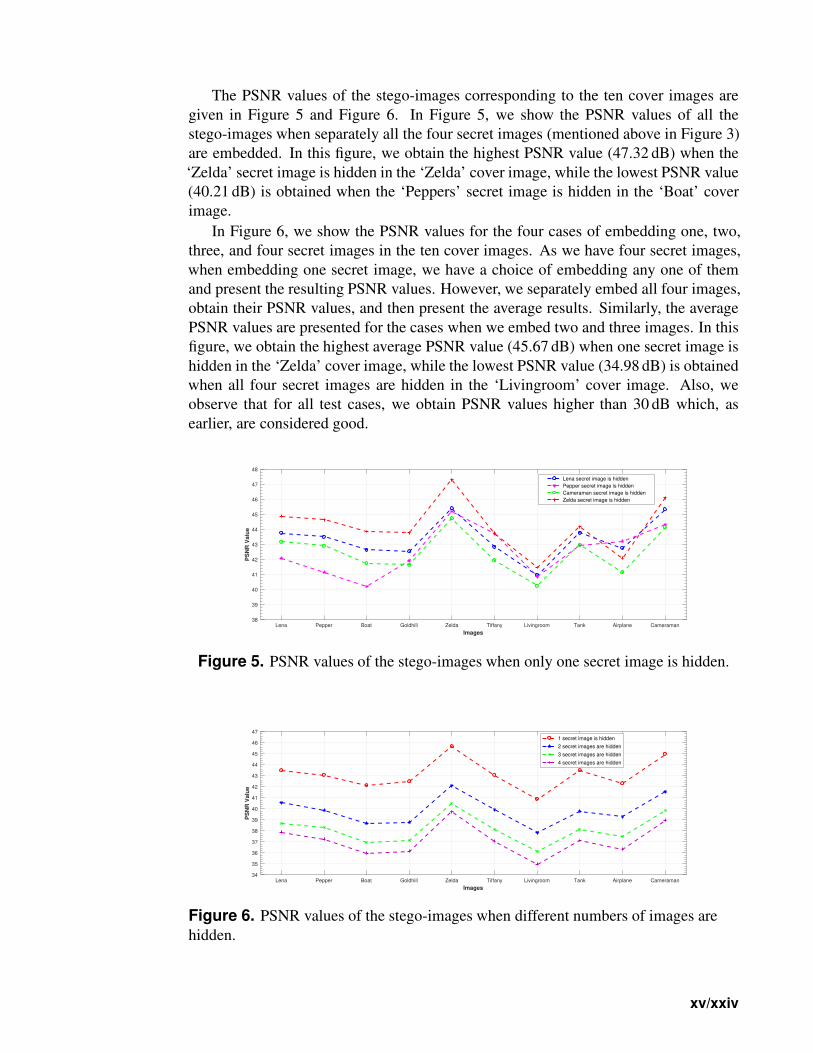
The PSNR values of the stego-images corresponding to the ten cover images are
given in Figure 5 and Figure 6. In Figure 5, we show the PSNR values of all the
stego-images when separately all the four secret images (mentioned above in Figure 3)
are embedded. In this figure, we obtain the highest PSNR value (47.32 dB) when the
‘Zelda’ secret image is hidden in the ‘Zelda’ cover image, while the lowest PSNR value
(40.21 dB) is obtained when the ‘Peppers’ secret image is hidden in the ‘Boat’ cover
image.
In Figure 6, we show the PSNR values for the four cases of embedding one, two,
three, and four secret images in the ten cover images. As we have four secret images,
when embedding one secret image, we have a choice of embedding any one of them
and present the resulting PSNR values. However, we separately embed all four images,
obtain their PSNR values, and then present the average results. Similarly, the average
PSNR values are presented for the cases when we embed two and three images. In this
figure, we obtain the highest average PSNR value (45.67 dB) when one secret image is
hidden in the ‘Zelda’ cover image, while the lowest PSNR value (34.98 dB) is obtained
when all four secret images are hidden in the ‘Livingroom’ cover image. Also, we
observe that for all test cases, we obtain PSNR values higher than 30 dB which, as
earlier, are considered good.
Lena Pepper Boat Goldhill Zelda Tiffany Livingroom Tank Airplane Cameraman
Images
38
39
40
41
42
43
44
45
46
47
48
PS
NR
Valu
e
Lena secret image is hidden
Pepper secret image is hidden
Cameraman secret image is hidden
Zelda secret image is hidden
Figure 5. PSNR values of the stego-images when only one secret image is hidden.
Lena Pepper Boat Goldhill Zelda Tiffany Livingroom Tank Airplane Cameraman
Images
34
35
36
37
38
39
40
41
42
43
44
45
46
47
PS
NR
Valu
e
1 secret image is hidden
2 secret images are hidden
3 secret images are hidden
4 secret images are hidden
Figure 6. PSNR values of the stego-images when different numbers of images are
hidden.
xv/xxiv

3.2.2 Other Numerical Measures
Mean Structural Similarity (MSSIM) Index This is an image quality assessment met-
ric used to measure the structural similarity between two images, which is most no-
ticeable to humans (Habib et al., 2016; Elzeki et al., 2021). MSSIM between the cover
image I and the stego-image SI is given as
MSSIM(I,SI) =1
M
M
∑j=1
SSIM(i j,si j), (11)
where i j and si j are the content of the cover image and the stego-image, respectively,
at the jth local window with M being the number of local windows (Habib et al., 2016;
Wang et al., 2004), and
SSIM(x,y) =(2µxµy +C1)(2σxy +C2)
(µ2x +µ2
y +C1)(σ 2x +σ 2
y +C2), (12)
where for vectors x and y, µx is the weighted mean of x, µy is the weighted mean of y,
σx is the weighted standard deviation of x, σy is the weighted standard deviation of y,
σxy is the weighted covariance between x and y, C1 and C2 are positive constants.
We take M = 1069156, C1 = (0.01× 255)2, and C2 = (0.03× 255)2 based upon
the recommendations from (Habib et al., 2016; Wang et al., 2004). The value of the
MSSIM index lies between 0 and 1, where the value 0 indicates that there is no struc-
tural similarity between the cover image and the corresponding stego-image, and the
value 1 indicates that the images are identical.
Normalized Cross-Correlation (NCC) Coefficient: This metric measures the amount
of correlation between two images (Parah et al., 2016). The NCC coefficient between
the cover image I and the stego-image SI is given as
NCC(I,SI) =∑r1
i=1 ∑r2j=1 I(i, j)SI(i, j)
∑r1i=1 ∑r2
j=1 I2(i, j), (13)
where r1 and r2 represent the row and column numbers of the image (for us either cover
or stego), respectively, and I(i, j) and SI(i, j) represent the pixel values of the cover
image and the stego-image, respectively. The NCC coefficient value of 1 indicates that
the cover image and the stego-image are highly correlated while a value of 0 indicates
that the two are not correlated.
Entropy: In general, entropy is defined as the measure of average uncertainty of a
random variable. In the context of an image, it is a statistical measure of randomness
that can be used to characterize the texture of the image (Gonzalez et al., 2004). For a
grayscale image (either a cover image or a stego-image in our case), entropy is given as
E =−255
∑i=0
(pi log2 pi), (14)
where pi ∈ [0,1] is the fraction of image pixels that have the value i. If the stego-image
is similar to its corresponding cover image, then the two should have similar entropy
values (due to similar textures).
xvi/xxiv

Normalized Absolute Error (NAE): This metric is a distance measure that captures
pixel-wise differences between two images (Arunkumar et al., 2019b). NAE between
the cover image I and the stego-image SI is given as
NAE(I,SI) =∑r1
i=1 ∑r2j=1 (|CI (i, j)−SI (i, j) |)
∑r1i=1 ∑r2
j=1CI (i, j), (15)
where r1 and r2 represent the row and the column numbers of the image (for us either
cover or stego), respectively, and CI(i, j) and SI(i, j) represent the pixel values of the
cover image and the stego-image, respectively. NAE has values in the range 0 to 1.
A value close to 0 indicates that the cover image is very close to its corresponding
stego-image, and a value close to 1 indicates that the two are substantially far apart.
In Table 4, we present the values of MSSIM index, NCC coefficient, entropy and
NAE for our SABMIS scheme when hiding all four secret images. We do not present
the values for the cases of embedding less than four secret images as their results will
be better than those given in Table 4. Hence, our reported results are for the worst case.
From this table, we observe that all values of the MSSIM index are nearly equal to 1
(different in the sixth place of decimal), the values of NCC coefficients are close to
1, and values of NAE are close to 0. The entropy values of the cover and the stego-
images are almost identical. All these values indicate that the cover images and their
corresponding stego-images are almost identical.
Table 4. MSSIM index, NCC coefficient, entropy, and NAE of the stego-images
when compared with the corresponding cover images.
Cover
ImageMSSIM NCC
EntropyNAE
Cover
Image
Stego-
Image
Lena 1 0.9992 7.443 7.463 0.009
Pepper 1 0.9997 7.573 7.598 0.012
Boat 1 0.9998 7.121 7.146 0.012
Goldhill 1 0.9998 7.471 7.486 0.013
Zelda 1 0.9964 7.263 7.272 0.011
Tiffany 1 0.9999 6.602 6.628 0.006
Livingroom 1 0.9996 7.431 7.438 0.013
Tank 1 0.9998 6.372 6.405 0.014
Airplane 1 0.9972 6.714 6.786 0.015
Cameraman 1 1.0000 7.055 7.123 0.009
Average 1 0.9991 7.104 7.1343 0.011
3.3 Secret Image Quality Assessment
Since human observers are considered the final arbiter to assess the quality of the ex-
tracted secret images, we compare one such original secret image and its corresponding
extracted secret image. The results of all other combinations are almost the same. In
Figures 7a and 7d, we show the original ‘Peppers’ secret image and the extracted ‘Pep-
pers’ secret image (from the ‘Zelda’ stego-image). From these figures, we observe that
there is very little distortion in the extracted image. Besides this, for these two images,
we also present their corresponding histograms (in Figures 7b and 7e, respectively), and
xvii/xxiv

edge map diagrams (in Figures 7c and 7f, respectively). Again, we observe minimal
variations between the original and the extracted secret images.
3.4 Security Analysis
The SABMIS scheme is a transform domain based technique which employs an indirect
embedding strategy, i.e., it does not follow the Least Significant Bit (LSB) flipping
method, and hence, it is immune to statistical attacks (Westfeld and Pfitzmann, 2000;
Yu et al., 2009). Moreover, in the SABMIS scheme, the measurement matrix Φ, and
the embedding/ extraction algorithmic settings are considered as secret-keys, which are
shared between the sender and the legitimate receiver. It is assumed that these keys are
not known to the eavesdropper. Hence, we achieve increased security in our proposed
system.
To justify this, we extract the secret image in two ways, i.e., by using correct secret-
keys and by using wrong secret-keys. Since the measurement matrix, which we use
(random matrix having numbers with mean 0 and standard deviation 1) is one of the
most commonly used measurement matrix and the eavesdropper can easily guess it, we
use this same measurement matrix while building wrong secret-keys. Here, we use the
same dimension of this matrix as well, i.e., p3× p2. In reality, the guessed matrix size
would be different from the original matrix size, which would make the extraction task
of the eavesdropper more difficult.
The algorithmic settings that we use will be completely unknown to the eavesdrop-
per. These involve using few constants (α = 0.01, β = 0.1, γ = 1 and c = 6) and a
set of cover image coefficients where secret image coefficients are embedded (using p1
and p4). While building wrong secret-keys, we take the common guess of one for all
constants (i.e., α = 1, β = 1, γ = 1 and c = 1) without changing the rest of the settings
(i.e., same p1 and p4). In reality, the eavesdropper would not be able to correctly guess
these other settings as well resulting in a further challenges during extraction.
We compare the average NAE values (between the original secret images and the
corresponding extracted ones) for both these cases. These values are presented in Fig-
ure 8. In this figure, we see that for correct secret-keys, the NAE values are close to 0,
and the for wrong secret-keys, the NAE values are very high. Hence, in the SABMIS
scheme, a change in secret-keys will lead to a shift in the accuracy between the origi-
nal secret images and their corresponding extracted ones, in turn, making our scheme
secure.
Moreover, in Figure 9 (a) and (b), we compare the ‘Peppers’ secret image when
extracted using correct and wrong secret-keys (from the ‘Zelda’ stego-image), respec-
tively. From this figure, we see that when using correct secret-keys, the visual distortion
in the extracted secret image is negligible, and when using the wrong secret-keys, the
distortion in the extracted secret image is very high (it is almost black).
3.5 Performance Comparison
We compare our SABMIS scheme with the existing steganography schemes (discussed
in the Introduction section) for the embedding capacity, the quality of stego-images, and
resistance to steganographic attacks. For the stego-image quality comparison, since
most works have computed PSNR values only, we use only this metric for analysis.
Further, resistance to steganographic attacks is not experimented by most of the past
xviii/xxiv

(a) ‘Peppers’ Original Secret Image
(OSI)
0
500
1000
1500
2000
2500
3000
0 50 100 150 200 250
(b) OSI Histogram
(c) OSI Edge Map
(d) ‘Peppers’ Extracted Secret Image
(ESI)
0
500
1000
1500
2000
2500
3000
0 50 100 150 200 250
(e) ESI Histogram
(f) ESI Edge Map
Figure 7. Visual quality analysis between the ‘Peppers’ original secret image and the
‘Peppers’ extracted secret image (from the ‘Zelda’ stego-image).
xix/xxiv

Lena Peppers Boat Goldhill Zelda Living room Tiffany Tank Airplane Camera man
Cover Image Used for Embedding
0
0.1
0.2
0.3
0.4
0.5
0.6
0.7
0.8
0.9
1
Ave
rag
e N
AE
Val
ues
Using correct secret-keysUsing wrong secret-keys
Figure 8. Average NAE value between the four original secret images and their
corresponding extracted secret images when using correct and wrong secret-keys.
(a) ‘Peppers’ extracted secret image
(using correct secret-keys)
(b) ‘Peppers’ extracted secret image
(using wrong secret-keys)
Figure 9. Visual quality analysis between the ‘Peppers’ extracted secret image using
correct and wrong secret-keys (from the ‘Zelda’ stego-image).
xx/xxiv

Table 5. Performance comparison of our SABMIS scheme with various other
steganography schemes.
Numbers
of
secret
images
Steganography SchemeType of
secret image
Type of
cover images
Embedding
capacity
(in bpp)
PSNR
(in dB)
Resistant
to stegan-
ographic
attacks?
1(Arunkumar et al., 2019b) Binary Grayscale 0.25 49.69 Yes
SABMIS Grayscale Grayscale 2 43.15 Yes
2(Hemalatha et al., 2013) Grayscale Color 1.33 44.75 Yes
SABMIS Grayscale Grayscale 4 39.83 Yes
3(Guttikonda et al., 2018) Binary Grayscale 2 46.36 No
SABMIS Grayscale Grayscale 6 38.12 Yes
4 SABMIS Grayscale Grayscale 8 37.14 Yes
works. Rather, they have just stated whether their scheme has such a property or not.
Hence, we use this information for comparison. Finally, although we check the quality
of the extracted secret images by comparing them with the corresponding original secret
images (as earlier), this check is not common in the existing works. Hence, we do not
perform this comparison.
As mentioned in the introduction, because of the lack of past work of embedding
grayscale secret images into a grayscale cover image, we compare with the cases of
embedding binary images into a grayscale image or embedding grayscale images into
a color image. Both these problems are easier than our problem.
This comparison is given in Table 5. As evident from this table, our scheme outper-
forms the competitive schemes in embedding capacity for the three cases of embedding
one, two, and three secret images. We do have a slight loss in the quality of the stego-
images. However, as earlier, this is considered acceptable because we are compromis-
ing very little in quality while gaining a lot more in embedding capacity. Moreover,
PSNR values over 30 dB are considered good (Gutub and Shaarani, 2020; Zhang et al.,
2013; Liu and Liao, 2008). Further, our scheme, like most of the other competitive
schemes (not all; please see (Guttikonda et al., 2018)), is resistant to steganographic
attacks. Finally, we are the first ones to embed four secret images in a cover image.
4 CONCLUSIONS AND FUTURE WORK
Securing secret information over Internet-based applications becomes important as il-
legitimate users try to access them. One way to secure this data is to hide them into
an image as the cover media, known as image steganography. Here, the challenges are
increasing the embedding capacity of the scheme, maintaining the quality of the stego-
image, and ensuring that the scheme is resistant to steganographic attacks. We propose
a blind multi-image steganography scheme for securing secret images in cover images
to substantially overcome all the three challenges. All our images are grayscale, which
is a hard problem.
First, we perform sampling of the cover image to obtain four sub-images. Further,
we sparsify (using DCT) each sub-image and obtain its sparse linear measurements
using a random measurement matrix. Then, we embed DCT coefficients of the secret
images into these linear measurements using our novel embedding rule. Second, we
xxi/xxiv
construct the stego-image from these modified measurements by solving the resulting
LASSO problem using ADMM. Third, using our proposed extraction rule, we extract
the secret images from the stego-image. We call this scheme SABMIS (Sparse Approx-
imation Blind Multi-Image Steganography). Using these components together helps
us to embed up to four secret images into one cover image (instead of the common
embedding of two secret images).
We perform experiments on several standard grayscale images. We obtain embed-
ding capacities of 2 bpp (bits per pixel), 4 bpp, 6 bpp, and 8 bpp while embedding one,
two, three, and four secret images, respectively. These embedding capacities are higher
than all the embedding capacities obtained in the literature until now. Further, there is
with very little deterioration in the quality of the stego-image as compared to its cor-
responding cover image (measured by the above metrics). The quality of the original
secret images and their corresponding extracted secret images is also almost the same.
Further, due to our algorithmic design, our scheme is resistant to steganographic attacks
as well.
Next, we discuss the future work in this context. First, since we embed secret im-
ages in images, in the future we plan to embed the secret data into text, audio, and video.
Second, we plan to apply optimization techniques to improve the values of parame-
ters α,β ,γ , etc. used in the embedding and the extraction algorithms of the SABMIS
scheme. Third, we plan to extend this work to real-time applications such as hiding
fingerprint data, iris data, medical information of patients, and personal signatures.
ACKNOWLEDGEMENT
This work has been supported by the DAAD in the project ‘A new passage to India’
between IIT Indore and the Leibniz Universität Hannover.
REFERENCES
(Accessed: 22-10-2019a). Images Database.
https://homepages.cae.wisc.edu/~ece533/images/.
(Accessed: 22-10-2019b). Images Database.
http://imageprocessingplace.com/root_files_V3/image_databases.htm.
(Accessed: 22-10-2019). The USC-SIPI Images Database.
http://sipi.usc.edu/database/.
Agrawal, R. and Ahuja, K. (2021). CSIS: compressed sensing-based enhanced-
embedding capacity image steganography scheme. IET Image Processing,
15(9):1909–1925.
Arunkumar, S., Subramaniyaswamy, V., Ravichandran, K. S., and Logesh, R. (2019a).
RIWT and QR factorization based hybrid robust image steganography using block
selection algorithm for IoT devices. Journal of Intelligent & Fuzzy Systems,
35(5):4265–4276.
Arunkumar, S., Subramaniyaswamy, V., Vijayakumar, V., Chilamkurti, N., and Logesh,
R. (2019b). SVD-based robust image steganographic scheme using RIWT and DCT
for secure transmission of medical images. Measurement, 139:426–437.
Baluja, S. (2019). Hiding images within images. IEEE transactions on pattern analysis
and machine intelligence, 42(7):1685–1697.
xxii/xxiv

Boyd, S., Parikh, N., Chu, E., Peleato, B., and Eckstein, J. (2010). Distributed opti-
mization and statistical learning via the alternating direction method of multipliers.
Foundations and Trends in Machine Learning, 3(1):1–122.
Elzeki, O. M., Elfattah, M. A., Salem, H., Hassanien, A. E., and Shams, M. (2021). A
novel perceptual two layer image fusion using deep learning for imbalanced covid-19
dataset. PeerJ Computer Science, 7:e364.
Gabay, D. (1976). A dual algorithm for the solution of nonlinear variational prob-
lems via finite element approximation. Computers & Mathematics with Applications,
2(1):17–40.
Gonzalez, R. C., Woods, R. E., and Eddins, S. L. (2004). Digital image processing
using MATLAB. Pearson Education India.
Guttikonda, P., Cherukuri, H., and Mundukur, N. B. (2018). Hiding encrypted multi-
ple secret images in a cover image. In Proceedings of International Conference on
Computational Intelligence and Data Engineering, pages 95–104. Springer.
Gutub, A. and Shaarani, F. A. (2020). Efficient implementation of multi-image secret
hiding based on LSB and DWT steganography comparisons. Arabian Journal for
Science and Engineering, 45(4):2631–2644.
Habib, W., Sarwar, T., Siddiqui, A. M., and Touqir, I. (2016). Wavelet denoising of
multiframe optical coherence tomography data using similarity measures. IET Image
Processing, 11(1):64–79.
Hemalatha, S., Acharya, U. D., Renuka, A., and Kamath, P. R. (2013). A secure image
steganography technique to hide multiple secret images. In Computer Networks &
Communications (NetCom), pages 613–620. Springer.
Hwang, H. J., Kim, S., and Kim, H. J. (2016). Reversible data hiding using least
square predictor via the LASSO. EURASIP Journal on Image and Video Processing,
2016(1):42.
Kordov, K. and Zhelezov, S. (2021). Steganography in color images with random order
of pixel selection and encrypted text message embedding. PeerJ Computer Science,
7:e380.
Liu, C. L. and Liao, S. R. (2008). High-performance JPEG steganography using com-
plementary embedding strategy. Pattern Recognition, 41(9):2945–2955.
Maheswari, S. U. and Hemanth, D. J. (2017). Performance enhanced image steganog-
raphy systems using transforms and optimization techniques. Multimedia Tools and
Applications, 76(1):415–436.
Nardone, D., Ciaramella, A., and Staiano, A. (2019). A sparse-modeling based ap-
proach for class specific feature selection. PeerJ Computer Science, 5:e237.
Pal, A. K., Naik, K., and Agrawal, R. (2019). A steganography scheme on JPEG
compressed cover image with high embedding capacity. The International Arab
Journal of Information Technology, 16(1):116–124.
Pan, J. S., Li, W., Yang, C. S., and Yan, L. J. (2015). Image steganography based
on subsampling and compressive sensing. Multimedia Tools and Applications,
74(21):9191–9205.
Parah, S. A., Sheikh, J. A., Loan, N. A., and Bhat, G. M. (2016). Robust and blind
watermarking technique in DCT domain using inter-block coefficient differencing.
Digital Signal Processing, 53:11–24.
Sanjutha, M. K. (2018). An image steganography using particle swarm optimiza-
xxiii/xxiv

tion and transform domain. International Journal of Engineering & Technology,
7(224):474–477.
Srinivas, M. and Naidu, R. M. (2015). Sparse approximation of overdetermined sys-
tems for image retrieval application. In Agrawal, P., Mohapatra, R., Singh, U., and
Srivastava, H., editors, Mathematical Analysis and its Applications, volume 143,
pages 219–227. Springer.
Stallings, W. (2019). Cryptography and network security: principles and practice.
Prentice Hall.
Wang, Z., Bovik, A., Sheikh, H., and Simoncelli, P. (2004). Image quality assessment:
From error visibility to structural similarity. IEEE Transactions on Image Processing,
13(4):600–613.
Westfeld, A. and Pfitzmann, A. (2000). Attacks on steganographic systems. In Pfitz-
mann, A., editor, Information Hiding, volume 1768, pages 61–76. Springer.
Yu, L., Zhao, Y., Ni, R., and Zhu, Z. (2009). PM1 steganography in JPEG images using
genetic algorithm. Soft Computing, 13(4):393–400.
Zhang, Y., Jiang, J., Zha, Y., Zhang, H., and Zhao, S. (2013). Research on embedding
capacity and efficiency of information hiding based on digital images. International
Journal of Intelligence Science, 3(02):77–85.
xxiv/xxiv
