This article was downloaded by: [University of Limerick]On: 08 May 2013, At: 13:54Publisher: Taylor & FrancisInforma Ltd Registered in England and Wales Registered Number: 1072954 Registered office: Mortimer House,37-41 Mortimer Street, London W1T 3JH, UK

IIE TransactionsPublication details, including instructions for authors and subscription information:http://www.tandfonline.com/loi/uiie20

Fast-ship commitment contracts in retail supply chainsHao-Wei Chen a , Diwakar Gupta a & Haresh Gurnani ba Department of Industrial & Systems Engineering , University of Minnesota , Minneapolis ,MN , 55455 , USAb Department of Management, School of Business Administration , University of Miami , CoralGables , FL , 33124 , USAAccepted author version posted online: 16 Jul 2012.Published online: 29 Apr 2013.

To cite this article: Hao-Wei Chen , Diwakar Gupta & Haresh Gurnani (2013): Fast-ship commitment contracts in retail supplychains, IIE Transactions, 45:8, 811-825

To link to this article: http://dx.doi.org/10.1080/0740817X.2012.705449

PLEASE SCROLL DOWN FOR ARTICLE

Full terms and conditions of use: http://www.tandfonline.com/page/terms-and-conditions

This article may be used for research, teaching, and private study purposes. Any substantial or systematicreproduction, redistribution, reselling, loan, sub-licensing, systematic supply, or distribution in any form toanyone is expressly forbidden.

The publisher does not give any warranty express or implied or make any representation that the contentswill be complete or accurate or up to date. The accuracy of any instructions, formulae, and drug doses shouldbe independently verified with primary sources. The publisher shall not be liable for any loss, actions, claims,proceedings, demand, or costs or damages whatsoever or howsoever caused arising directly or indirectly inconnection with or arising out of the use of this material.

IIE Transactions (2013) 45, 811–825Copyright C© “IIE”ISSN: 0740-817X print / 1545-8830 onlineDOI: 10.1080/0740817X.2012.705449

Fast-ship commitment contracts in retail supply chains

HAO-WEI CHEN1, DIWAKAR GUPTA1,∗ and HARESH GURNANI2

1Department of Industrial & Systems Engineering, University of Minnesota, Minneapolis, MN 55455, USAE-mail: guptad@me.umn.edu2Department of Management, School of Business Administration, University of Miami, Coral Gables, FL 33124, USA

Received July 2010 and accepted May 2012

This article analyzes three types of supply contracts between a supplier and a retailer when both agree as follows—if a customerexperiences a stockout, then the purchased item can be shipped to the customer on an expedited basis at no extra cost. This practiceis referred to as the fast-ship option in this article. In the first contract (Structure A), the supplier specifies a total supply commitmentand allows the retailer to choose its split between the initial order and the amount left to satisfy fast-ship orders. In the other twocontracts (Structures B and C), the supplier agrees to fully supply the retailer’s initial order but places a restriction on the quantityavailable for fast-ship commitment. The difference between the second and third contracts is that in contract Structure B the suppliermoves first, whereas in contract Structure C the supplier determines its commitment after observing the retailer’s order. The supplier’sand the retailer’s optimal decisions and preferences are characterized. The question of how the supplier and the retailer may resolvetheir conflict regarding the preferred contract type is addressed.

[Supplementary materials are available for this article. Go to the publisher’s online edition of IIE Transactions for proofs.]

Keywords: Supply contracts, fast-ship option, stockouts, partial backorders, newsvendor model

1. Introduction

A stockout occurs when supply falls short of demand.Stockouts are not uncommon in retail supply chains (Gruenet al. (2002) report a worldwide average out-of-stock rate of8.3%) that often results in customer dissatisfaction (Grantand Fernie, 2008). In industries such as toys and apparel,matching supply with demand is especially challenging dueto fast-changing customer preferences and market trends,which lead to high inventory costs, markdowns, and lostsales (Johnson, 2001). The options available to customerswhen they experience stockouts affect the profits of supplychain partners.

When customers learn that the retail store they are in hasrun out of a desired item, they may respond in a number ofdifferent ways. Some customers may switch brands and buya substitute product, others may buy from a different retailstore, and some others may postpone purchase decision orchoose an entirely different product (Emmelhainz et al.,1991). Such stockout-triggered purchasing behaviors mayhurt retailers even when some customers purchase sub-stitutes because stockout events can negatively affect theoverall sales of products in the same category due to lackof selections available to customers (Kalyanam et al., 2007).

∗Corresponding author

Retailers’ profit margins in many industry segments are low(for example, see Datamonitor (2008) for electronics indus-try profile and profit margins of key players), which sug-gests that cost-effective means of capturing sales that arelost during stockout events would be of interest to retailers.

To reduce loss of sales during stockout periods, retailersmay negotiate a flexible supply contract that allows themto either adjust the order size before the start of the sell-ing season or to place multiple orders during the sellingseason. The latter includes offering a fast-ship option tocustomers, which is the focus of this study. A retailer thatoffers the fast-ship option arranges to have out-of-stockitems shipped directly from the supplier to customers at noadditional cost to the customers, thereby creating a hybridbetween traditional and drop-ship channels. For example,Best Buy, an electronic products’ retailer, offers an InstantShip option to in-store customers when mobile devices theyintend to purchase are not available in store. Many apparelretailers, such as J. Crew and Gap Inc., offer to home-shipitems when customers cannot find desired items in the rightsizes on the store shelf, absorbing the shipping cost. OfficeDepot ships ink and toner cartridges free to customers if itruns out of such items.

The fast-ship option allows the channel to use theretailer-held inventory as the primary source of supply(traditional approach) and supplier-held backup inventoryas the secondary source of supply (drop-ship approach).

0740-817X C© 2013 “IIE”

Dow

nloa

ded

by [

Uni

vers

ity o

f L

imer

ick]

at 1

3:54

08

May

201

3

812 Chen et al.

The latter is used only when the primary source is ex-hausted. This contrasts with the two extremes of tradi-tional and drop-ship channels in which all inventory is kepteither at the retailer’s location or at the supplier’s location(Wilson, 2000). Drop-ship channels are commonly encoun-tered in the context of Internet-based retailers (e.g., Zappos,an Internet footwear store). Similarly, the supplier may alsoprocure additional inventory at a higher cost to replenishits stock as needed.

In the traditional approach, the retailer bears all of the in-ventory cost and its stocking decision determines channelperformance. Use of the drop-ship approach reduces re-tailers’ inventory cost. However, this option does not meetthe needs of those customers who prefer to touch and feelthe items before buying and those who do not want towait. In fact, depending on the product, between 47 and92% of retail sales happen in “brick-and-mortar” stores(Schonfeld, 2010). The fast-ship option combines the ad-vantages of both traditional and drop-ship channels andprovides a mechanism by which supply–demand mismatchcost may be apportioned between the retailer and the sup-plier. Models presented in this article show that the fast-ship option has the potential to improve profits of both theretailers and the suppliers.

In a channel that supports the fast-ship option, both theretailer and the supplier have two opportunities to replen-ish. The retailer places an initial order before the start ofthe selling season and multiple fast-ship orders that occurlater in the selling season. The fast-ship orders are placed,as needed, after inventory at the retail store runs out. Simi-larly, the supplier procures (or produces) a certain quantityof items before the selling season, which can be greater thanthe retailer’s initial order size, and may procure additionalitems after demand realization, if needed.

From a retailer’s perspective, the fast-ship option maybe particularly attractive for high-value items for which theobsolescence cost is high and the additional cost of directshipping to customers is relatively low. This is because thefast-ship option can reduce the retailer’s cost of meetingits demand. A supplier who cooperates with the retailerto support the fast-ship option may also benefit from thispractice because the total sales may be higher. However,because the retailer may decrease its initial order size andthe procurement cost for the fast-ship orders may be higher,suppliers may wish to limit the fast-ship commitment viathe terms of a supply contract.

In this article, we compare three possible supply commit-ment contract structures between a single supplier (S) anda single retailer (R) that support the fast-ship option for aproduct with a short selling season. Within each structure,a particular set of values of the retailer’s and the supplier’sparameters is referred to as a contract. These three struc-tures are variants of quantity flexibility provisions that arecommon in supply contracts. We describe related literatureat a later point in this section.

In the first structure (referred to as Structure A contract),the supplier commits to a maximum total quantity p ≥ 0.

The retailer can then choose any initial order quantity q andplace any number of fast-ship requests as long as the totalamount ordered does not exceed p. The second structure,referred to as Structure B, limits only the supplier’s fast-ship commitment. That is, the supplier commits to supplyno more than z ≥ 0 via the fast-ship option. It also suppliesany amount q ordered by the retailer before the start of theselling season. Both A and B are supplier-driven structuresbecause the supplier makes its choice first and the retailerorders q after learning either p or z. The third structure,referred to as Structure C, may be viewed as a retailer-led analog of Structure B because the supplier choosesits fast-ship commitment γ after receiving R’s initialorder q.

The three contract structures belong to a family of affinesupply commitment contracts in which the supplier’s totalcommitment is an affine function of the form aq + b, anda and b are contract parameters. Different values of a andb give rise to different relationships between the initial or-der size and the fast-ship supply commitment. Specifically,a Structure A contract arises when a = 1 and b = p − q,whereas Structures B and C arise when a = 1 and b is eitherz or γ . The actual number of items that are fast shippeddepends on the parameter values chosen by the two playersin each supply structure.

The setting in our article is motivated by contractual re-strictions, also referred to as vertical restraints (Rey andVerge, 2005). While different types of vertical restraintshave been studied in the literature (Rey and Tirole, 1986),we consider variants of quantity fixing contracts, which in-clude minimum quantity purchases, quantity forcing, aswell as quantity rationing contracts. Our focus is on spe-cific forms of quantity rationing contracts where the sup-plier imposes restrictions on the quantity available to thebuyer. In particular, the three structures are variants ofseveral quantity fixing contracts used in practice. For ex-ample, the Indefinite Delivery, Indefinite Quantity (ID/IQ)contracts offered by suppliers to government agencies aresimilar to Structure A (see http://www.gsa.gov/portal/content/103926). The ID/IQ contract specifies a maxi-mum total quantity that would be purchased within a fixedtime period. The buyer can place multiple orders and eachorder can be of an arbitrary size. However, orders mustbe placed during the contract period and the negotiatedprice applies to the orders whose cumulative quantity isless than the maximum specified in the contract. Similarly,in a practice similar to Structures B and C, state govern-ment agencies require suppliers of road salt (used for de-icing roads during winter) to agree to supply more than theamount initially ordered at the negotiated price (e.g., BART(2008)). The supplier caps extra supplies at values that areproportional to the initial order quantity. The ID/IQ androad salt supply contracts are similar in spirit, though notexactly the same, as the three structures studied in thisarticle.

We develop mathematical models that help explainhow the supplier and the retailer would choose values of

Dow

nloa

ded

by [

Uni

vers

ity o

f L

imer

ick]

at 1

3:54

08

May

201

3

Fast-ship commitment contracts 813

their parameters within each contract structure when theymaximize their individual profits. Specifically, we estab-lish certain properties of the retailer’s and the supplier’sparameter optimization problems that allow us to solvethese problems using non-linear optimization techniques.We then compare the three contracts under optimal param-eter choices to determine which structure is preferred bythe supplier and which structure is preferred by the retailer.Within reasonable ranges of problem parameters, we showthat from the supplier’s viewpoint, B is the most preferredstructure and A is the least preferred when both the sup-plier and the retailer make individually optimal decisions.This is because the retailer orders less up front under Struc-ture A contract and fast-ship sales are less profitable for thesupplier. As a result, among the two supplier-led structures,the supplier will not offer Structure A, even though A mayprovide greater flexibility to the retailer. Structure B is moreprofitable than C for the supplier because the supplier re-ceives a larger initial order in Structure B as compared withstructure C.

From the retailer’s perspective, Structure A is usually pre-ferred, except in cases where the total promised supply (p)is smaller than the promised supply under other contractstructures (i.e., p is less than either q + z or q + γ ). How-ever, because Structure A will not be chosen by the supplier,we compare only Structures B and C from the retailer’sperspective. We show that when the retailer faces a choicebetween Structures B and C, it prefers Structure C becauseit can secure a greater supply commitment under Struc-ture C as compared with B. We also test whether contractstructure preference changes if the supplier (resp. retailer)chooses the wholesale price in supplier-led (resp. retailer-led) contracts.

Clearly, the two players have different contract structurepreferences, which gives rise to the problem of contract-type selection. We present two approaches for resolvingsuch differences. In the first case, one of the two players isassumed to be the dominant player (hold-out). The behav-ior of a hold-out player can be explained as follows. Whenthe retailer is the hold-out, it would only accept a contractin which its profit is at least as much as its best profit undercontract Structure C. Similarly, when the supplier is thehold-out, it would only accept a contract in which its profitis at least as much as its best profit under contract StructureB. The profits of the two players in this case are referred toas hold-out profits.

The second case arises when there is no dominant playerand neither player can insist on a minimum profit thresh-old equal to its optimal profit under its preferred contractstructure. Instead, the two players are willing to negotiateand each player has a disagreement profit level. For the re-tailer, the disagreement profit level is the best profit it wouldmake under contract Structure B and for the supplier, thedisagreement profit level is the profit it would make un-der contract Structure C. This is because the retailer (resp.

supplier) is guaranteed to strike a contract if it agrees toStructure B (resp. C).

For the first case, we show that the player who is notthe hold-out player can propose a contingent contract thatimproves its profit over its hold-out profit while maintain-ing or improving the hold-out player’s profit. In the secondcase with no hold-out player, we prove the existence of ne-gotiated contracts, which guarantee that each player willmake more than its disagreement profit. We do not dwellon the division of profits because many solutions are pos-sible depending on the negotiating power of each party.However, we show that under a negotiated contract, it is ineach player’s best interest to maximize total supply chainprofit; i.e., the negotiation approach is equivalent to ver-tical integration of the two players and contract structurepreferences become irrelevant. These two conflict resolvingapproaches remain valid when the wholesale price is cho-sen by the leader in the contract. Specifically, this means thewholesale price is determined by the supplier in StructureB and the retailer in Structure C.

We also briefly discuss the effect of partial backorderrate. Specifically, we observe that a higher partial backo-rder rate is beneficial for the supplier in Structure B andfor the retailer in Structure C. For other cases, the resultsdepend on parameters. However, it is more likely that bothplayers can benefit from the higher partial backorder rate inStructure C.

1.1. Related literature

Supply contracts are widely used in industry (e.g., Whiteet al. (2005)) and commitment flexibility, similar to that im-plied by the three contract structures we study, is a commontheme in the supply contracts’ literature; see, for example,Van Mieghem (2003), Wu et al. (2005), and Stevenson andSpring (2007). Quantity Flexibility (QF) allows the buyerto adjust the purchase quantity in a certain range withoutpenalty, reducing the channel’s cost of matching supply anddemand (Wu, 2005).

In a QF contract, the buyer announces an early tentativeorder qT before the production period begins. Knowing qT,the supplier commits to supply qS. After receiving a moreaccurate demand forecast, which occurs before the sellingseason starts, the buyer then adjusts its order size and comesup with a final (firm) order qF. The buyer (resp. supplier)is not penalized if qF ≥ qT − a (resp. qS ≥ min{qF, (qT +b)}), where a and b are called flexibility parameters (see, e.g.,Tsay (1999)). That is, the buyer in a QF contract commitsto purchasing no less than a certain amount/percentagebelow the forecast and the seller commits to supply up to acertain amount/percentage above the forecast.

The supply commitment contracts we study serve a dif-ferent purpose than QF contracts. The fast-ship optionis triggered only after stockout occurs and its purpose isto provide a mechanism for serving unmet demand. In

Dow

nloa

ded

by [

Uni

vers

ity o

f L

imer

ick]

at 1

3:54

08

May

201

3

814 Chen et al.

contrast, the reason for allowing quantity adjustments inQF contracts is to reduce the expected cost of overage andshortage. QF contracts do not help retailers meet demandthat occurs after stockouts. Another difference is that fast-ship sales induce additional costs for both the supplier andthe retailer in our supply commitment contracts, whereasin QF contracts, quantity adjustments within permissibleranges do not induce additional costs. Finally, supply flex-ibility parameters are often exogenously determined in QFcontracts; for example, a ≥ 0 and b ≥ −a are exogenous inTsay (1999). In our setting, within each contract structure,the supply commitment is determined by parameters p, z,or γ , which are chosen by the supplier, and both playerspick individually optimal contract parameters.

Structure A contract is also related to the two-periodstochastic dynamic programming model of a backup agree-ment contract proposed by Eppen and Iyer (1997a). In thefirst period, the buyer commits to buy up to some amountqT for the selling season and claims immediate ownershipof (1 − σ )qT units where σ is exogenous. After period 1demand is realized, the buyer can adjust its inventory byplacing a second order of up to σqT units at the originalprice in period 2. In each period, a small portion of salesis returned and a constant fraction of returned units canbe reused to satisfy demand. In addition, the buyer pays apenalty � for any reserved units that are not purchased.

Our approach is similar because we also allow the re-tailer to place a second order up to some pre-determinedtotal quantity commitment by the supplier. However, ourproblem is different because (i) the total supply commit-ment is a decision made by the supplier in our modelsand consequently the buyer does not pay a penalty for notpurchasing all of the promised supply; (ii) we model boththe supplier’s and the retailer’s problems and obtain theiroptimal parameters, whereas Eppen and Iyer do not ad-dress the supplier’s problem; and (iii) Eppen and Iyer focuson the impact of backup fraction σ and penalty � on thebuyer’s expected profit and commitment qT, whereas westudy the interactions between the supplier and the retailerfor three different contract structures when both playersmake individually optimal decisions within each structure.

Our model is also related to previous works involvingmore than one replenishment opportunity; see, for exam-ple, Eppen and Iyer (1997b), Gurnani and Tang (1999),and Donohue (2000). These authors study the use of twoordering opportunities for fashion products when bothopportunities arise prior to the start of the selling sea-son. The retailer, after placing an initial order, observes asignal that is correlated with the demand during the sell-ing period. With this new information, the demand fore-cast is updated and the second replenishment is used tolower supply–demand mismatch costs. The focus of thepapers cited above is to model the effect of the retailer get-ting additional (but incomplete) demand information afterplacing its first order. In contrast, in our setting, the pur-pose of the second replenishment (which takes place after

demand realization) is to serve customers that agree to waitfor out-of-stock items (see Gupta et al. (2010) for similarsettings).

The dual strategy model in Netessine and Rudi (2006) isalso related to our model. When dual strategy is adopted,each retailer uses its stockpile as the primary source of itemsneeded to satisfy demand and drop shipping as a backupsource when its stock runs out. However, there are impor-tant differences between our work and Netessine and Rudi(2006). First, Netessine and Rudi (2006) assume that whenin-store inventory runs out, all remaining customers agreeto receive their items from the drop-ship channel, whichcorresponds to setting α = 1 in our model. Our model ismore general and can be applied to situations in which somecustomers do not take advantage of the fast-ship option.Second, the supplier in our model has two replenishmentopportunities, whereas the supplier in Netessine and Rudi(2006) has a single replenishment opportunity. Put differ-ently, the scenario discussed in Netessine and Rudi is aspecial case in our model. Netessine and Rudi (2006) com-pare the dual strategy with both pure traditional (i.e., wherez or γ = 0) and pure drop-ship (i.e., where q = 0) environ-ments. In contrast, we analyze different contract structureswithin which the fast-ship commitment level is chosen bythe supplier. Netessine and Rudi (2006) identify the bestchannel strategy as a function of supply chain parameters,whereas we provide insights into supply chain partners’contract structure preferences and parameter choices.

The rest of this article is organized as follows. Notationand model formulations for the three contract structuresare introduced in Section 2. We analyze the two player’soptimal decisions for Structures A and B in Section 3 andStructure C in Section 4. In Section 5, we contrast the threestructures from the retailer’s and the supplier’s perspectivesand address the problem of contract structure selection.Section 6 discusses the effect of leader-selected wholesaleprice and the effect of different values of partial backorderrate. A summary of the main results and directions forfuture research are provided in Section 7. All proofs arepresented in an Online Supplement within the publisher’sonline edition of IIE Transactions.

2. Notation and model formulation

The sequence of events for the three contract structures isillustrated in Fig. 1. The retailer offers the fast-ship optionuntil the available fast-ship commitment (as guaranteedvia its contract with the supplier) is exhausted. StructuresA and B are supplier-led contracts and commitments p andz are decided before the retailer decides the order quantity.Structure C is a retailer-led contract in which commitmentγ is decided after the retailer’s order quantity decision.

The notation used in model formation is listed in Table 1.R’s demand X ∈ R+ is continuous with probability densityand distribution functions f (·) and F(·), respectively. We

Dow

nloa

ded

by [

Uni

vers

ity o

f L

imer

ick]

at 1

3:54

08

May

201

3

Fast-ship commitment contracts 815

Table 1. Summary of notation

Notation Description

Decision variables:p S’s total commitment under Structure A, p ≥ 0z S’s fast-ship commitment under Structure B,

z ≥ 0γ S’s fast-ship commitment under Structure C,

γ ≥ 0y S’s extra production quantityq R’s order quantity, q ≥ 0Parameters:X Demand with density and distribution functions

f (·) > 0 and F(·)α Partial backorder rate, α ∈ [0, 1]y Additional units procured during the first

replenishment, y ≥ 0w Wholesale price per unit for regular orders,

w ≥ c1 + τ1

δ Markup per unit for fast-ship orders, δ ≥ 0w2 Wholesale price per unit for the fast-ship orders,

w2 = w + δ

τ1, τ2 Regular/fast-ship order shipping cost per unit,τ1, τ2 ≥ 0

c1, c2 S’s first/second replenishment costs per unit,c1, c2 ≥ 0

h Holding cost incurred by S for stocking eachextra unit, h ≥ 0

r Retail price per unit, r ≥ 0

also assume that f (·) > 0 over the support of X. Note thatonly a fraction of customers utilize the fast-ship option(referred to as the partial backorder rate in this article), andthe rest do not make a purchase at the retailer’s store. This issimilar to partial backorders where the retailer backordersonly when a customer is willing to wait (see, for example,Abad (1996)). The supplier procures q + y items beforethe selling season and may procure additional items duringthe selling season as needed. The supplier’s replenishmentcosts are c1 and c2 for the two replenishment options. Thesupplier pays a holding cost h for the additional y units itprocures because these items are sold only at the end of theselling period. The supplier replenishes during the sellingseason only when y cannot satisfy all promised fast-shiporders.

The shipping costs for regular and fast-ship orders areτ1 and τ2, respectively. Both τ1 and τ2 are paid by the sup-plier to a third-party logistics service provider. Note that τ1and τ2 are independent of origin and destination becauseshipping charges depend on the item’s size and/or weightbut not origin and destination. Such pricing schemes arecommon in the United States see, for example, U.S. PostalService’s (www.usps.com) shipping rates for standard-sizedboxes of certain maximum weight regardless of origin anddestination. The retailer sells items to customers at a unitretail price r regardless of whether the item is sold fromon-hand inventory or by using the fast-ship option. Thesupplier sells items to the retailer at a unit wholesale pricew for initial orders and w + δ for fast-ship orders; thatis, the wholesale price for fast-ship items is obtained byadding a mark-up δ ≥ 0 to the base price w and markupsof 15–20% are common (Scheel, 1990). For notational sim-plification, we also use w2 = w + δ to denote the wholesaleprice of fast-ship items.

Parameters r , w, and δ are assumed exogenous in this ar-ticle. Scenarios with endogenous w are discussed in Section6. In addition, we make the following assumptions aboutkey parameters.

Assumption 1. τ1 ≤ τ2.

Assumption 2. c1 ≤ c2.

Assumption 3. c1 + h ≤ c2.

Assumption 1 reflects the fact that fast-ship orders utilizepremium shipping (more expensive) with expedited deliv-ery, whereas regular orders are sent to retailers utilizing aneconomical transportation system. Assumption 2 impliesthat the second batch procurement cost is higher than thefirst because suppliers have shorter time windows withinwhich to obtain the second replenishment. Conditionalupon needing an item to satisfy excess demand, Assump-tion 3 makes it cheaper for the supplier to procure this itemin the first batch and hold it until the end of the sellingseason. Although our model remains valid without As-sumption 3, it serves to make h relevant because otherwisethe supplier would not stock extra units and no holdingcost would be incurred.

Supplier chooses p Retailer chooses q Up to p − q fast-ship orders are supported

Supplier chooses z Retailer chooses q Up to z fast-ship orders are supported

Supplier chooses γRetailer chooses q Up to γ fast-ship orders are supported

Structure A

Structure B

Structure C

Demand realization

Fig. 1. The sequence of events for the contract structures A, B, and C.

Dow

nloa

ded

by [

Uni

vers

ity o

f L

imer

ick]

at 1

3:54

08

May

201

3

816 Chen et al.

We also assume that parameters are chosen such that thefast-ship option is attractive to both the supplier and theretailer, which is ensured by the following two assumptions

Assumption 4. w < r − δ.

Assumption 5. w − τ1 − c1 ≥ α(w2 − τ2 − c1 − h) ≥ 0.

Assumption 4 ensures that both initial and fast-shiporders are profitable for the retailer. In absence of this re-quirement, the retailer may choose not to offer the fast-ship option to customers when a stockout occurs. Becausew2 ≥ w (i.e., δ ≥ 0) and the retail price does not changewhen items are supplied via the fast-ship option, the re-tailer’s unit profit is greater if an item is supplied fromstock. Assumption 5 is a sufficient condition under whichthe fast-ship orders are also less profitable for the supplier.If this condition were violated, the supplier might not sup-ply orders before the start of the selling season and offeran infinite fast-ship commitment under all three contractstructures, which would obviate the need to study differentcontract structures. That is, Assumption 5 identifies a rangeof problem parameters within which the questions posedin this paper are non-trivial. We explain the logic behindAssumption 5 in the following paragraph.

The supplier’s contribution margin from a sale from thefirst replenishment is (w − τ1 − c1) and at most α(w2 −τ2 − c1 − h) from the second replenishment. This is be-cause only α fraction of customers would purchase the itemwhen experiencing stockout. Therefore, if w − τ1 − c1 ≥α(w2 − τ2 − c1 − h) ≥ 0, then the supplier definitely earnsmore from each unit ordered by the retailer in its ini-tial order. Two scenarios arise when Assumption 5 isviolated. If w − τ1 − c1 < α(w2 − τ2 − c2), then we canshow that the three structures are identical and the sup-plier would choose p, z, and γ = ∞ because fast-ship or-der produces higher profits. However, if α(w2 − τ2 − c2) <

w − τ1 − c1 ≤ α(w2 − τ2 − c1 − h), then we are not able toobtain results analytically because the marginal benefitsfor both types of orders depend on other parameters. Nu-merically, we observe that there exists a threshold betweenα(w2 − τ2 − c2) and α(w2 − τ2 − c1 − h) such that our re-sults hold if (w − τ1 − c1) is greater than the threshold.Later in Sections 3 and 4 we show that w2 ≥ τ2 + c2 is suf-ficient for p∗ = γ ∗ = ∞ within Structures A and C but thatz∗ is not necessarily unbounded under the same condition.

Because the expedited transportation cost is linear in thenumber of fast-ship items, modeling several fast-ship or-ders as a single second replenishment does not affect theprofit functions of the two players. In other words, thetotal fast-ship demand can be represented as α(x − q)+,where b+ = max(0, b). Let index i ∈ {A, B, C} denote thecontract structure. In expressions that apply to all contractstructures, we use parameter j ∈ {p, z, γ } to denote sup-ply commitment. The retailer’s expected profit given that

contract structure i has been selected, supplier has commit-ted j , and retailer has ordered q can be written as follows:

π iR(q, j ) = r E[X ∧ q] − wq + (r − w2)E[α(X − q)+

∧ ζ ij (q)], (1)

where (X ∧ q) denotes min(X, q), and ζ ij (q) is the maximum

fast-ship supply committed by S. That is, ζ ij (q) = p − q, or

z, or γ when (i, j ) = (A, p), (B, z), and (C, γ ), respectively.Moreover, r E[X ∧ q] − wq is the expected profit fromthe initial order, (α(X − q)+ ∧ ζ i

j (q)) is the magnitude offast-ship demand and (r − w2)E[α(X − q)+ ∧ ζ i

j (q)] is theexpected profit from the fast-ship orders. Equation (1) as-sumes that both players have made their decisions. The op-timal values of decision variables depend on the sequencein which the two players make their decisions, but the re-sulting profit for the retailer after decisions are made canbe expressed as Equation (1) for all contract types.

Similarly, given that contract structure i has been se-lected, the retailer has ordered q, and the supplier has cho-sen y and j , the supplier’s expected profit is given by

π iS(y, j, q) = (w − τ1 − c1)q − (c1 + h)y + (w2 − τ2)

× E[α(X − q)+ ∧ ζ i

j (q)]

− c2 E[(α(X − q)+−y)+ ∧ (ζ i

j (q)−y)+]

. (2)

In Equation (2), (w − τ1 − c1)q is the profit from R’s ini-tial order, (c1 + h)y is the cost of procuring and stock-ing extra y items, and (w2 − τ2)E[α(X − q)+ ∧ ζ i

j (q)] isthe revenue from fast-ship demand. The last term comesfrom the fact that S has an uncovered commitment of(ζ i

j (q) − y)+ and the leftover fast-ship demand after stock-pile y is exhausted equals (α(X − q)+ − y)+. Therefore,c2 E[(α(X − q)+ − y)+ ∧ (ζ i

j (q) − y)+] is the extra procure-ment cost for the fast-ship orders that are not served fromthe amount stocked by the supplier in response to the re-tailer’s initial order. Similar to Equation (1), Equation (2)also assumes that both players have made their decisions.Although the optimal values of either player’s decision vari-ables depend on the sequence of events, the resulting profitof the supplier can be expressed as Equation (2) for allcontract types.

In Structures A and B, the supplier is the firstmover. Therefore, when (i, j ) ∈ {(A, p), (B, z)}, the re-tailer’s problem is to find qi ( j ) = arg max π i

R(q, j ) foreach supplier-selected j , whereas the supplier’s prob-lem is to find yi ( j ) = arg max π i

S(y, j, qi ( j )) and j∗ =arg max j π i

S(yi ( j ), j, qi ( j )). In contrast, the retailer is thefirst mover in Structure C. Therefore, the supplier’s prob-lem in Structure C is to find yC(q) = arg maxy πC

S (y, γ, q)and γ (q) = arg maxγ πC

S (yC(q), γ, q) for each retailer-selected q, whereas the retailer’s problem is to find qC =arg maxq πC

R (q, γ (q)).With Equations (1) and (2) in hand, we are ready to

find optimal parameter values for each player under eachcontract structure. In the ensuing analysis, we use ei

j (q).=

Dow

nloa

ded

by [

Uni

vers

ity o

f L

imer

ick]

at 1

3:54

08

May

201

3

Fast-ship commitment contracts 817

q + ζ ij (q)/α for notational convenience and assume, with-

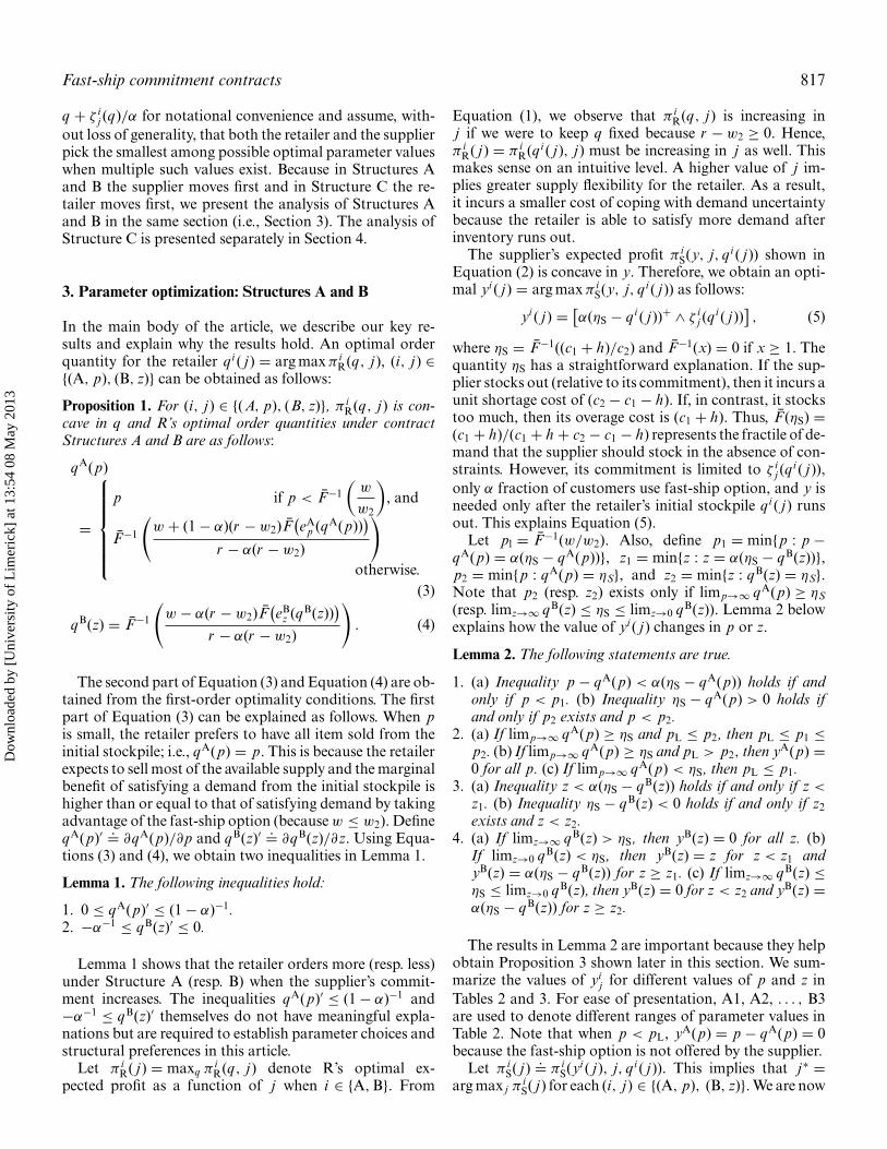
out loss of generality, that both the retailer and the supplierpick the smallest among possible optimal parameter valueswhen multiple such values exist. Because in Structures Aand B the supplier moves first and in Structure C the re-tailer moves first, we present the analysis of Structures Aand B in the same section (i.e., Section 3). The analysis ofStructure C is presented separately in Section 4.

3. Parameter optimization: Structures A and B

In the main body of the article, we describe our key re-sults and explain why the results hold. An optimal orderquantity for the retailer qi ( j ) = arg max π i

R(q, j ), (i, j ) ∈{(A, p), (B, z)} can be obtained as follows:

Proposition 1. For (i, j ) ∈ {(A, p), (B, z)}, π iR(q, j ) is con-

cave in q and R’s optimal order quantities under contractStructures A and B are as follows:

qA(p)

=

⎧⎪⎪⎪⎪⎪⎨⎪⎪⎪⎪⎪⎩

p if p < F−1

(w

w2

), and

F−1

(w + (1 − α)(r − w2)F

(eA

p (qA(p)))

r − α(r − w2)

)

otherwise.(3)

qB(z) = F−1

(w − α(r − w2)F

(eB

z (qB(z)))

r − α(r − w2)

). (4)

The second part of Equation (3) and Equation (4) are ob-tained from the first-order optimality conditions. The firstpart of Equation (3) can be explained as follows. When pis small, the retailer prefers to have all item sold from theinitial stockpile; i.e., qA(p) = p. This is because the retailerexpects to sell most of the available supply and the marginalbenefit of satisfying a demand from the initial stockpile ishigher than or equal to that of satisfying demand by takingadvantage of the fast-ship option (because w ≤ w2). DefineqA(p)′ .= ∂qA(p)/∂p and qB(z)′ .= ∂qB(z)/∂z. Using Equa-tions (3) and (4), we obtain two inequalities in Lemma 1.

Lemma 1. The following inequalities hold:

1. 0 ≤ qA(p)′ ≤ (1 − α)−1.2. −α−1 ≤ qB(z)′ ≤ 0.

Lemma 1 shows that the retailer orders more (resp. less)under Structure A (resp. B) when the supplier’s commit-ment increases. The inequalities qA(p)′ ≤ (1 − α)−1 and−α−1 ≤ qB(z)′ themselves do not have meaningful expla-nations but are required to establish parameter choices andstructural preferences in this article.

Let π iR( j ) = maxq π i

R(q, j ) denote R’s optimal ex-pected profit as a function of j when i ∈ {A, B}. From

Equation (1), we observe that π iR(q, j ) is increasing in

j if we were to keep q fixed because r − w2 ≥ 0. Hence,π i

R( j ) = π iR(qi ( j ), j ) must be increasing in j as well. This

makes sense on an intuitive level. A higher value of j im-plies greater supply flexibility for the retailer. As a result,it incurs a smaller cost of coping with demand uncertaintybecause the retailer is able to satisfy more demand afterinventory runs out.

The supplier’s expected profit π iS(y, j, qi ( j )) shown in

Equation (2) is concave in y. Therefore, we obtain an opti-mal yi ( j ) = arg max π i

S(y, j, qi ( j )) as follows:

yi ( j ) = [α(ηS − qi ( j ))+ ∧ ζ i

j (qi ( j ))

], (5)

where ηS = F−1((c1 + h)/c2) and F−1(x) = 0 if x ≥ 1. Thequantity ηS has a straightforward explanation. If the sup-plier stocks out (relative to its commitment), then it incurs aunit shortage cost of (c2 − c1 − h). If, in contrast, it stockstoo much, then its overage cost is (c1 + h). Thus, F(ηS) =(c1 + h)/(c1 + h + c2 − c1 − h) represents the fractile of de-mand that the supplier should stock in the absence of con-straints. However, its commitment is limited to ζ i

j (qi ( j )),

only α fraction of customers use fast-ship option, and y isneeded only after the retailer’s initial stockpile qi ( j ) runsout. This explains Equation (5).

Let pl = F−1(w/w2). Also, define p1 = min{p : p −qA(p) = α(ηS − qA(p))}, z1 = min{z : z = α(ηS − qB(z))},p2 = min{p : qA(p) = ηS}, and z2 = min{z : qB(z) = ηS}.Note that p2 (resp. z2) exists only if limp→∞ qA(p) ≥ ηS(resp. limz→∞ qB(z) ≤ ηS ≤ limz→0 qB(z)). Lemma 2 belowexplains how the value of yi ( j ) changes in p or z.

Lemma 2. The following statements are true.

1. (a) Inequality p − qA(p) < α(ηS − qA(p)) holds if andonly if p < p1. (b) Inequality ηS − qA(p) > 0 holds ifand only if p2 exists and p < p2.

2. (a) If limp→∞ qA(p) ≥ ηS and pL ≤ p2, then pL ≤ p1 ≤p2. (b) If limp→∞ qA(p) ≥ ηS and pL > p2, then yA(p) =0 for all p. (c) If limp→∞ qA(p) < ηS, then pL ≤ p1.

3. (a) Inequality z < α(ηS − qB(z)) holds if and only if z <

z1. (b) Inequality ηS − qB(z) < 0 holds if and only if z2exists and z < z2.

4. (a) If limz→∞ qB(z) > ηS, then yB(z) = 0 for all z. (b)If limz→0 qB(z) < ηS, then yB(z) = z for z < z1 andyB(z) = α(ηS − qB(z)) for z ≥ z1. (c) If limz→∞ qB(z) ≤ηS ≤ limz→0 qB(z), then yB(z) = 0 for z < z2 and yB(z) =α(ηS − qB(z)) for z ≥ z2.

The results in Lemma 2 are important because they helpobtain Proposition 3 shown later in this section. We sum-marize the values of yi

j for different values of p and z inTables 2 and 3. For ease of presentation, A1, A2, . . . , B3are used to denote different ranges of parameter values inTable 2. Note that when p < pL, yA(p) = p − qA(p) = 0because the fast-ship option is not offered by the supplier.

Let π iS( j ) .= π i

S(yi ( j ), j, qi ( j )). This implies that j∗ =arg max j π i

S( j ) for each (i, j ) ∈ {(A, p), (B, z)}. We are now

Dow

nloa

ded

by [

Uni

vers

ity o

f L

imer

ick]

at 1

3:54

08

May

201

3

818 Chen et al.

Table 2. Values of yA(p)

Scenario Conditions Range of p Value of yA(p)

A1 limp→∞ qA(p) ≥ ηS and p2 ≤ pL p ∈ [0, pL) yA(p) = p − qA(p) = 0

p ∈ [pL,∞) yA(p) = 0A2 lim

p→∞ qA(p) ≥ ηS and p2 > pL p ∈ [0, pL) yA(p) = p − qA(p) = 0p ∈ [pL, p1) yA(p) = p − qA(p)p ∈ [p1, p2) yA(p) = α(ηS − qA(p))p ∈ [p2,∞) yA(p) = 0

A3 limp→∞ qA(p) < ηS p ∈ [0, pL) yA(p) = p − qA(p) = 0

p ∈ [pL, p1) yA(p) = p − qA(p)p ∈ [p1,∞) yA(p) = α(ηS − qA(p))

ready to solve for j∗. Let qi ( j )′ denote the rate of change inq as a function of j . We first point out a sufficient conditionin Proposition 2 in which the supplier does not restrict itstotal commitment under contract Structure A. This hap-pens when w2 ≥ c2 + τ2.

Proposition 2. If w2 ≥ c2 + τ2, then p∗ is unbounded.

When w2 ≥ c2 + τ2, the supplier can earn a positive profitfrom fast-ship orders even if it does not produce any ex-tra quantity up front (i.e., y = 0). As a result, there is noeconomic reason for the supplier to limit the size of itscommitment. One may be tempted to extend this intu-ition to contract Structure B. That is, to expect that whenw2 ≥ c2 + τ2, the supplier always chooses z∗ = ∞. As weshow below, the above result may not always hold forStructure B.

Next, we prove that the supplier’s profit under StructuresA and B is unimodal in p and z for exponential and uni-form demand distributions. A profit-maximizing value of pcan be unbounded as seen in Proposition 2, but the optimalvalue of z is always finite. In addition to these distributions,we studied Gaussian and gamma distributions numerically(the latter with shape parameter ≥ 1) and found that theresult in Proposition 3 held in all of our numerical experi-ments. In the following, we shall assume that the supplier’sprofit under Structures A and B is unimodal. Note that theresults presented in the rest of this article do not depend ona particular demand distribution as long as unimodality ofsupplier’s profit function holds.

Proposition 3. If the demand is either exponentially or uni-formly distributed, then the following two statements aretrue:

1. The supplier’s profit under a Structure A contract has atmost one local maximum. The global maximizer p∗ iseither equal to the local maximizer or p∗ is unbounded.

2. The supplier’s profit under a Structure B contract hasat most one local maximum. The global maximizer z∗ iseither equal to the local maximizer, or z∗ = 0, or z∗ isunbounded.

Proposition 3 implies that the optimal p (resp. z) canbe obtained efficiently via simple line searches and by com-paring the supplier’s profit at the local maximizer with thatat p = ∞ (resp. z = 0 or ∞). Note that when w2 ≥ c2 + τ2,the supplier can earn additional profit by satisfying fast-ship demand beyond its commitment specified in contractterms. However, the retailer would then anticipate greateravailability and lower its initial order, which would lowerthe supplier’s profit. Hence, the supplier has an incentiveto uphold contract terms and supply no more than itscommitment.

Before closing this section, we present a comparison ofStructures A and B in terms of their impact on the retailer’sstocking decision. Recall that 0 ≤ qA(p)′ ≤ (1 − α)−1 and−α−1 ≤ qB(z)′ ≤ 0, which shows that R responds differ-ently within the two structures if the supplier were toincrease available supply—q is non-decreasing in p andnon-increasing in z. The different responses come fromdifferent ways in which the retailer can react to changesin supply commitments under Structures A and B. These

Table 3. Values of yB(z)

Scenario Conditions Range of z Value of yB(z)

B1 limz→∞ qB(z) > ηS z ∈ [0,∞) yB(z) = 0

B2 limz→0

qB(z) < ηS z ∈ [0, z2) yB(z) = zz ∈ [z1,∞) yB(z) = α(ηS − qB(z))

B3 limz→∞ qB(z) ≤ ηS ≤ lim

z→0qB(z)) z ∈ [0, zθ ) yB(z) = 0

z ∈ [z2,∞) yB(z) = α(ηS − qB(z))

Dow

nloa

ded

by [

Uni

vers

ity o

f L

imer

ick]

at 1

3:54

08

May

201

3

Fast-ship commitment contracts 819

observations also provide greater insights into the relativesize of initial orders; see Proposition 4.

Proposition 4. For any p and z, qA(p) ≤ qB(z).

Proposition 4 shows that independent of contract pa-rameter values within each structure, the supplier receivesa larger initial order under Structure B as compared to A.This result is used to establish the preference of the supplierfor Structure B over A in Proposition 8.

4. Parameter optimization: Structure C

In Structure C, the supplier chooses γ after knowing q.Recall that the extra supply y is chosen by the supplier afterobserving q in all three structures. Because πC

S (y, γ, q) isconcave in y (proof is omitted for brevity), it can be shownthat the supplier chooses yC according to

yC(q) = [α(ηS − q)+ ∧ γ ]. (6)

Let ηR = F−1((c1 + h)/(w2 − τ2)). We obtain γ (q) =arg maxγ πC

S (yC(q), γ, q) in the following Proposition 5.

Proposition 5. The supplier’s profit πCS (yC(q), γ, q) is either

unbounded or unimodal in γ . In addition, the optimal γ (q)can be obtained as follows:

γ (q) ={∞ if w2 ≥ c2 + τ2,

α(ηR − q)+ otherwise. (7)

The quantity ηR can be explained in a manner similar to ηS.The reason that c2 does not appear in the expression for ηRis that when w2 < c2 + τ2, the supplier always selects y = γ

and there is no need to obtain more items at unit cost c2.Next, we obtain an optimal order quantity, qC =

arg maxq πCR (q, γ (q)), as shown in the following Proposi-

tion 6. Hereafter, we use πCR (q) = πC

R (q, γ (q)) and πCS (q) =

πCS (yC(q), γ (q), q) for convenience.

Proposition 6. The retailer’s profit is bimodal in q andthere exists a c1 ∈ [w(w2 − τ2)/r-h, w(w2 − τ2)/(r − α(r −w2)) − h] such that the optimal order quantity qC can beobtained as follows:

qC =

⎧⎪⎪⎪⎪⎨⎪⎪⎪⎪⎩

F−1

(w

r − α(r − w2)

)if either w2 ≥ c2 + τ2, or

w2 < c2 + τ2 and c1 ≤ c1,

F−1(w

r

)if w2 <c2 + τ2 and c1 > c1.

(8)

The intuition behind Proposition 6 is as follows. When ei-ther the wholesale price is sufficiently large (w2 ≥ c2 + τ2)or the unit cost of the supplier’s initial purchase is suffi-ciently small (w2 < c2 + τ2 and c1 ≤ c1), the supplier makesan ample fast-ship commitment to the retailer. In such

cases, the retailer’s decision is based upon an assumptionof ample availability of fast-ship supply. That is, the vastmajority of customers who exercise the fast-ship optionare served in this case. However, when w2 < c2 + τ2 andc1 > c1, the supplier chooses a conservative value of γ (q)because its second replenishment cost is higher. Anticipat-ing this response, the retailer orders more up front.

Note that when qC = F−1(w/r ) and γ (qC) = 0, a Struc-ture C contract is identical to a Structure B contract withz∗ = 0. Similarly, when w2 ≥ c2 + τ2, Structures A and Care identical because qA = qC and p − qA = γ (qC) = ∞.That is, in some cases, the ability to be the first to choosecontract parameters (also called market leadership) doesnot affect either party’s expected profit. Equation (7) andProposition 6 also help obtain the following inequalities.

Proposition 7. For a fixed pair of (w, δ) values, the followinginequalities hold.

1. qA(p) ≤ qC for any p;2. γ (q) ≥ z∗ where q = qB(z∗);3. qB(z) ≥ qC where z = γ (qC).

The arguments that lead to Part 1 of Proposition 7 aresimilar to those presented immediately after Proposition4. Because the retailer enjoys greater freedom to adjustthe supply between initial order and fast-ship orders undercontract Structure A, it is not required to commit to anorder quantity as large as that in contract Structure C. Theintuition behind Part 2 of Proposition 7 is that because thesupplier chooses γ after knowing qC, it can commit to ahigher supply than that under Structure B without worry-ing about the possibility that a higher supply commitmentmay induce the retailer to order less up front. For simi-lar reasons, the retailer chooses a smaller order quantityunder Structure C when the fast-ship supply commitmentunder Structure C is the same as that under Structure B(Part 3 of Proposition 7). Proposition 7 is important be-cause it leads to key results related to contract structurepreferences (Proposition 8) and the possibility of resolvingconflict (Proposition 9) in Section 5.

5. Contract structure preference and selection

We first investigate which contract structures are preferredby each player. In Proposition 8, we show that the supplierweakly prefers Structure B contracts and the retailer weaklyprefers Structure A contracts unless the total promised sup-ply under Structure A is lower than that under the othertwo contract types. In Proposition 8, the relationship “�”denotes a weak preference.

Proposition 8. For a fixed pair of (w, δ) values, the followingstatements are true:

Dow

nloa

ded

by [

Uni

vers

ity o

f L

imer

ick]

at 1

3:54

08

May

201

3

820 Chen et al.

1. The supplier’s preference ordering of contract structuresis B � C � A.

2. If the total promised supply under Structure A is at leastas much as that under Structures B and C, then the retailerprefers A.

3. When Structure A is unavailable, the retailerprefers C � B.

Proposition 8 can be explained by first observing thatfor the same total supply commitment, the supplier’s profitis higher within a contract structure that induces the re-tailer to order more up front. This is because higher initialpurchase quantity simultaneously increases initial sales rev-enue and reduces the need for fast-ship supply, which canbe costly to the supplier. Conversely, the retailer’s profit ishigher when a contract structure allows it to order slightlyless up front without sacrificing supply commitment orelse when a structure allows it to obtain a greater fast-shipsupply commitment for the same initial purchase quantity.From Proposition 3 and Part 1 of Proposition 7, we observethat the retailer orders less when Structure A is utilized, re-gardless of the supplier’s total commitment. Therefore, itis clear that Structure A is the least preferred structure forthe supplier. Moreover, from Part 3 of Proposition 7, weobserve that when supply commitment is held the same, theretailer orders more under Structure B than Structure C.This explains the preference ordering of contract structuresfrom the supplier’s viewpoint. Within supplier-led struc-tures, B � A even when w is chosen by the supplier withinthe constraint that w ≤ r − δ for each fixed δ.

We consider the retailer’s viewpoint next. If the total sup-ply under Structure A is no less than that under the othertwo structures, it is clear that this would be the preferredstructure for the retailer because the retailer can choose toorder less up front. In other words, although the retailer isthe first mover in Structure C, Structure A provides greaterflexibility as long as the supply is sufficient. We also provedin Proposition 8 that the retailer prefers Structure C overB because the retailer can secure greater supply commit-ment for the same initial purchase quantity. Therefore, Rprefers Structure C to B even when it has the right to choosewholesale price (see details in Section 6).

5.1. Contract structure selection

We observed above that between the two supplier-led struc-tures, the supplier prefers B over A. Therefore, a supplierwill not select A as long as the option to select B is available.We also observed that among Structures B and C, the sup-plier prefers B, whereas the retailer prefers C. This createsa potential conflict. In this section, we discuss how suchconflict may be resolved.

We present two approaches for resolving conflict in con-tract selection preferences. The contract resolution ap-proach depends on whether one player is dominant overthe other. First, we show that when there is a dominant

(hold-out) player, the other player can offer a modifiedcontract to increase its profit without hurting the hold-outplayer’s profit. Second, we show that when there is no hold-out player, that is, both players have equal power, they canuse a bargaining framework to decide the split of profit be-tween themselves such that both players’ profits are higherthan their disagreement profits.

5.1.1. Scenarios with a hold-out playerIf the channel has a hold-out player, then this means thatthe hold-out player will cooperate only if its profit equalsits maximum profit under its preferred contract structure.However, this may lead to a lower profit for the otherplayer. We argue next that as a non-hold-out player, ei-ther the supplier or the retailer may offer a modified con-tract that improves its profit and simultaneously make theother player weakly prefer the modified contract. We showbelow that such recourse is always available. In Proposi-tion 9, z∗ (resp. qC) is the optimal choice of supplier’s (resp.retailer’s) decision variable under contract Structure B(resp. C).

Proposition 9.

1. There exists a z ≥ z∗ such that πBR(z) ≥ πC

R (qC) andπB

S (z) ≥ πCS (qC).

2. There exists a q ≥ qC such that πBR(z∗) ≤ πC

R (q) andπB

S (z∗) ≤ πCS (q).

The results in Proposition 9 can be explained as follows.If the retailer is the hold-out player and it strictly prefersthe Structure C contract, then the supplier may offer ahigher supply commitment only if the retailer agrees to thechoice of Structure B to ensure that the retailer earns aslightly higher profit under modified B than that under C.In addition, the order quantity under the modified Struc-ture B contract (accepted by the retailer) can be proven tobe higher than that under Structure C contract (argumentsare similar to those underlying Part 3 of Proposition 7).Therefore, the modified Structure B contract is still a bet-ter choice for the supplier. Similarly, if the supplier is thehold-out player, the retailer can find a q ≥ qC such thatthe modified Structure C contract is preferred by both thesupplier and the retailer. This happens because the supplycommitment under modified Structure C contract remainshigher than z∗ (arguments are similar to Part 2 of Proposi-tion 7).

Next, we use an example to illustrate the results shownin Proposition 9. Consider a case in which X is gamma dis-tributed with E[X] = 400 and Var(X) = 8000. Other prob-lem parameters are r = 12, w = 8, w2 = 10.5, τ1 = 0.1,τ2 = 2, c1 = 1, c2 = 9, h = 0, and α = 0.5. The results areshown in Tables 4 and 5.

The first rows of Tables 4 and 5 show both parties’ prof-its and preferences when each makes an individually opti-mal decision. That is, z∗ = 70.5 and qC = 346. As shown

Dow

nloa

ded

by [

Uni

vers

ity o

f L

imer

ick]

at 1

3:54

08

May

201

3

Fast-ship commitment contracts 821

Table 4. Example of conflict resolution by providing modified contracts when the supplier is the hold-out player and the retailer offersmodified contract C

z q B(z) γ (q) q π BS (z) π B

R (z) πCS (qC) πC

R (qC)

Individual optimum 70.5 348.5 81.0 346.0 2610.7 1265.8 2601.0 1267.8R’s counter-offer — — 79.52 349.0 — — 2614.4 1267.6

in Proposition 8, the supplier prefers B and the retailerprefers C. In the second row of Table 4, we present a mod-ified Structure C contract when the retailer commits to ahigher-than-optimal order quantity. We see that when theretailer increases qC from 346 to 349, both parties prefer themodified C contract over B. In this example, the retailer’sprofit increases from 1265.8 to 1267.6 and the supplier’sprofit increases from 2610.7 to 2614.4. The retailer’s profitis only slightly less than its best profit of 1267.8, whichwould be realized under Structure C.

Similarly, if the supplier offers a modified B contract byincreasing z from 70.5 to 85, results are shown in Table 5. Inthis example, both players prefer the modified B contract ascompared with the original C contract. The retailer’s profitincreases from 1267.8 to 1268.6 and the supplier’s profitincreases from 2601.0 to 2608.0. Note that the modifiedcontracts B and C also generate greater channel profitscompared with the original contracts.

5.1.2. Scenarios without a hold-out playerSuppose there is no hold-out player. In this case, eachplayer has a minimum profit expectation, referred to as thedisagreement profit. We define disagreement profits next.Because the supplier’s profit is greater under contract Struc-ture B and the retailer’s profit is greater under Structure C,the disagreement profits (minimum profit each party ex-pects to earn) are πB

R(z∗) and πCS (qC) for the retailer and

the supplier, respectively. We call these disagreement profitsbecause the retailer (resp. the supplier) can always earn aminimum of πB

R(z∗) (resp. πCS (qc) by agreeing to the selec-

tion of contract Structure B (resp. C).Let π i

T(q, y, j ) denote the total supply chain profit ina negotiated profit allocation scheme when both playersagree to use contract structure i ∈ {B, C} and 0 < σS < 1(resp. σR = 1 − σS) denote the supplier’s (resp. retailer’s)fraction of total profits; i.e., π i

S,T(q, y, j ) = σSπiT(q, y, j )

and π iR,T(q, y, j ) = σRπ i

T(q, y, j ). Because σS and σR donot depend on (q, y, j ), maximizing individual profit in anegotiated contract is equivalent to maximizing π i

T(q, y, j ).

That is, let

qi = arg maxq

π iR,T(q, y, j ) = σR arg max

qπ i

T(q, y, j ), (9)

and

(yi , j i ) = arg max(y, j )

π iS,T(q, y, j ) = σS arg max

(y, j )π i

T(qi , y, j ).

(10)

By the definition of (q, y, j ), we obtain π iT(q, y, j ) ≥

π iT(q, y, j ) for any (q, y, j ). Furthermore, the only differ-

ence between Structures B and C is the sequence of deci-sions. That is, πB

T (q, y, z) = πCT (q, y, γ ) if z = γ . Because

the decision sequence does not matter when the two play-ers agree to maximize total profits in the supply chain, itfollows that qB = qC and z = γ . In other words, when thetwo players decide to negotiate a profit sharing contract,Structure B and Structure C are identical and there is nocontract preference issue. The only question that remains iswhether a negotiated contract yields higher profit as com-pared each player’s disagreement profit. This question isanswered in the following proposition.

Proposition 10. There exists some (σR, σS) such thatπ i

S,T(q, y, j ) ≥ πCS (qC) and π i

R,T(q, y, j ) ≥ πBR(z∗).

Proposition 10 shows that the two players can always finda set of (σR, σS) such that a negotiated contract generatesa higher individual profit than each player’s disagreementprofit. That is, a conflict can be resolved as long as σ liesbetween σR and σS.

A contract satisfying Proposition 10 can result eitherfrom direct negotiation between the retailer and the sup-plier or when the two players trust this decision to athird-party arbiter. If the arbiter were to choose a profitallocation that lies outside the feasible range we identified(e.g., σ < σR or σ > σS), then a negotiated solution wouldnot exist because in that case one of the two players woulddo better by accepting the hold-out position of the otherplayer in the first place. That is, if one of the parties knowsthat it will not receive a fair share in a negotiated solution,

Table 5. Example of conflict resolution by providing modified contracts when the retailer is the hold-out player and the supplier offersmodified contract C

z q B(z) γ (q) qC π BS (z) π B

R (z) πCS (qC) πC

R (qC)

Individual optimum 70.5 348.5 81.0 346.0 2610.7 1265.8 2601.0 1267.8S’s counter-offer 85 347.6 — — 2608.0 1268.6 — —

Dow

nloa

ded

by [

Uni

vers

ity o

f L

imer

ick]

at 1

3:54

08

May

201

3

822 Chen et al.

Table 6. Example of conflict resolution by providing modified contracts when the supplier is the hold-out player and the retaileroffers modified contract C

w z q B(z) w γ (q) q π BS (z) π B

R (z) πCS (qC) πC

R (qC)

Original 9.5 786.4 325.7 1.1 0 523.3 3062.5 712.5 0 4166.6R’s offer — — — 9.5 754.2 333.5 — — 3065.1 714.4

then negotiation will not occur because this party can dobetter by accepting the hold-out position of the other party.

We demonstrate how such negotiation might workthrough an example. Using parameters introduced in Ta-bles 4 and 5, we observe that π i

T(q, y, j ) = 4218.7. Hence,any negotiated contract with σS ∈ [0.62, 0.7] should be ac-ceptable to the two players when there is no hold-out player.In particular, when σS = 0.65, the supplier earns 2742.2,which is greater than 2601.0 (profit under C). Similarly, theretailer earns 1476.5, which is greater than 1265.8 (profitunder B).

Note that the contract conflict still exists when w is cho-sen by the contract leader. In such scenarios, the two ap-proaches for resolving conflict also remain valid. We discussthose scenarios in Section 6.

6. Insights

6.1. Contract structure preferences and selection withendogenous w

In this section, we allow w to be chosen by the first mover ina contract. That is, w and z are simultaneously selected bythe supplier in Structure B. Similarly, w and q in StructureC are selected by the retailer before the supplier decidesγ . The purpose of these variants is to study whether thestructural results obtained when w was assumed exogenousremain intact. We do not consider cases in which δ is chosenby the supplier because it can be argued that the supplierwould then set δ = r − w. The retailer would make zeroprofit from fast-ship orders and all contracts would becomeheavily skewed in favor of the supplier.

6.1.1. Contract structure preferencesWhen w is exogenous, we showed that Structure A willnot be chosen by the supplier. We can argue that the sameresult holds when w is chosen by the supplier. Hence, weonly focus on Structures B and C in this section. Recallthat the supplier prefers Structure B over C for a fixed w

(see Proposition 8). Hence, the same ordering holds withendogenous w because the supplier’s profit for Structure Bis even higher when w for Structure B is also selected by thesupplier. Similarly, the retailer prefers Structure C over Bwhen it chooses w within Structure C. In other words, theconflict between the supplier’s and the retailer’s preferenceidentified in Proposition 8 still exists when the wholesaleprice is endogenous and the leader is endowed with pricingpower.

6.1.2. Contract selection with a hold-out playerUsing the same parameters that we used for the examplepresented in Tables 4 and 5, we demonstrate how the twoconflict-resolving approaches shown in Section 5.1 workwhen w is endogenous. In Tables 6 and 7, we show thatwhen there is a hold-out player, a counter-offer from thenon-hold-out player can make both players weakly preferthe modified contract to the hold-out contract. This meansthat the approach we obtained in Proposition 9 remainsintact for endogenous w as well. However, if the retaileris the hold-out and the wholesale price is endogenous, thesupplier’s profit may be zero in some cases. This is becausethe retailer may choose w = c1 + τ1 in Structure C. In suchcases, a counter-offer from the supplier does not improveeither player’s profit. This is illustrated in Table 7. Whenthe retailer is the hold-out, we observe that the supplier’sprofit remains zero and the retailer earns the entire supplychain profit of 4166.6 with or without a counter-offer.

6.1.3. Contract selection without a hold-out playerWhen there is no hold-out player and the wholesale priceis endogenous, we can always find a negotiated contract(with a profit allocation decided either by both players orby the third-party arbiter) that is acceptable to the twoplayers, which is similar to results shown in Proposition10. Using the same parameters used for the example withexogenous wholesale price, π i

T(q, y, j ) = 4218.7 and bothplayers earn more than their disagreement profits (e.g., zerofor the supplier and 712.5 for the retailer) when σS is inbetween [0, 0.83].

Table 7. Example of conflict resolution by providing modified contracts when the retailer is the hold-out player and the supplieroffers modified contract B

w z q B(z) w γ (q) q π BS (z) π B

R (z) πCS (qC) πC

R (qC)

Original 9.5 786.4 325.7 1.1 0 523.3 3062.5 712.5 0 4166.6S’s offer 1.1 0 523.3 — — — 0 4166.6 — —

Dow

nloa

ded

by [

Uni

vers

ity o

f L

imer

ick]

at 1

3:54

08

May

201

3

Fast-ship commitment contracts 823

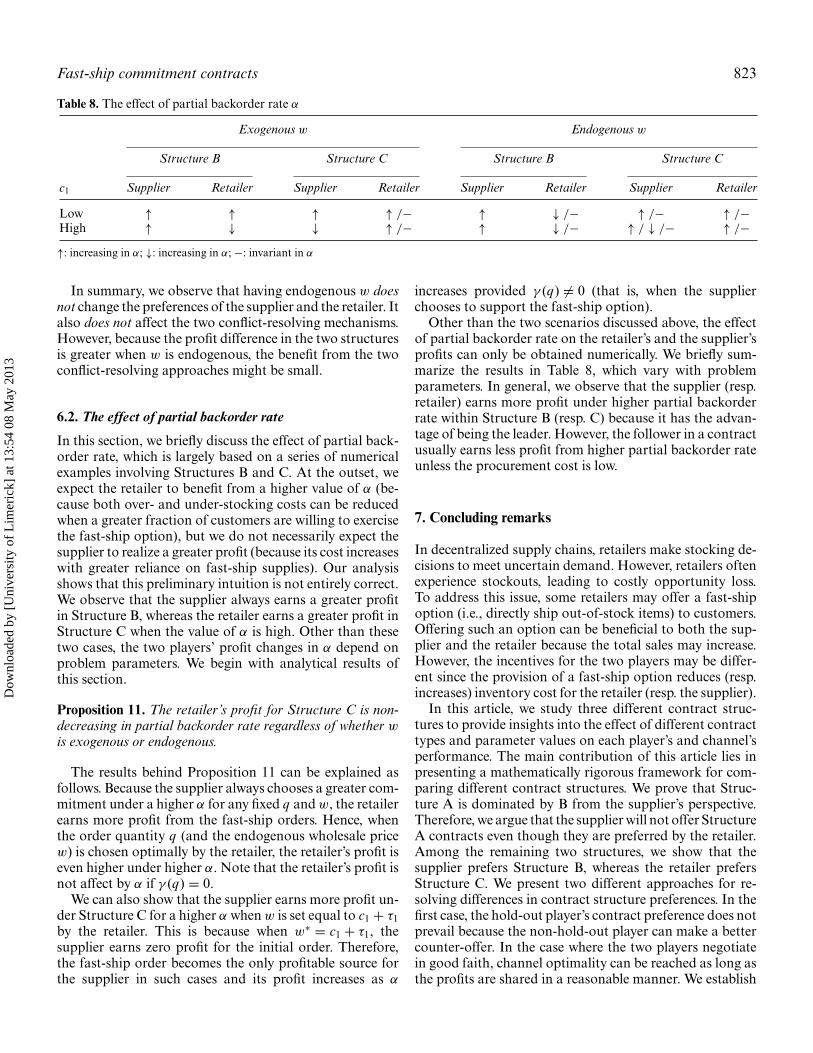
Table 8. The effect of partial backorder rate α

Exogenous w Endogenous w

Structure B Structure C Structure B Structure C

c1 Supplier Retailer Supplier Retailer Supplier Retailer Supplier Retailer

Low ↑ ↑ ↑ ↑ /− ↑ ↓ /− ↑ /− ↑ /−High ↑ ↓ ↓ ↑ /− ↑ ↓ /− ↑ / ↓ /− ↑ /−↑: increasing in α; ↓: increasing in α; −: invariant in α

In summary, we observe that having endogenous w doesnot change the preferences of the supplier and the retailer. Italso does not affect the two conflict-resolving mechanisms.However, because the profit difference in the two structuresis greater when w is endogenous, the benefit from the twoconflict-resolving approaches might be small.

6.2. The effect of partial backorder rate

In this section, we briefly discuss the effect of partial back-order rate, which is largely based on a series of numericalexamples involving Structures B and C. At the outset, weexpect the retailer to benefit from a higher value of α (be-cause both over- and under-stocking costs can be reducedwhen a greater fraction of customers are willing to exercisethe fast-ship option), but we do not necessarily expect thesupplier to realize a greater profit (because its cost increaseswith greater reliance on fast-ship supplies). Our analysisshows that this preliminary intuition is not entirely correct.We observe that the supplier always earns a greater profitin Structure B, whereas the retailer earns a greater profit inStructure C when the value of α is high. Other than thesetwo cases, the two players’ profit changes in α depend onproblem parameters. We begin with analytical results ofthis section.

Proposition 11. The retailer’s profit for Structure C is non-decreasing in partial backorder rate regardless of whether w

is exogenous or endogenous.

The results behind Proposition 11 can be explained asfollows. Because the supplier always chooses a greater com-mitment under a higher α for any fixed q and w, the retailerearns more profit from the fast-ship orders. Hence, whenthe order quantity q (and the endogenous wholesale pricew) is chosen optimally by the retailer, the retailer’s profit iseven higher under higher α. Note that the retailer’s profit isnot affect by α if γ (q) = 0.

We can also show that the supplier earns more profit un-der Structure C for a higher α when w is set equal to c1 + τ1by the retailer. This is because when w∗ = c1 + τ1, thesupplier earns zero profit for the initial order. Therefore,the fast-ship order becomes the only profitable source forthe supplier in such cases and its profit increases as α

increases provided γ (q) = 0 (that is, when the supplierchooses to support the fast-ship option).

Other than the two scenarios discussed above, the effectof partial backorder rate on the retailer’s and the supplier’sprofits can only be obtained numerically. We briefly sum-marize the results in Table 8, which vary with problemparameters. In general, we observe that the supplier (resp.retailer) earns more profit under higher partial backorderrate within Structure B (resp. C) because it has the advan-tage of being the leader. However, the follower in a contractusually earns less profit from higher partial backorder rateunless the procurement cost is low.

7. Concluding remarks

In decentralized supply chains, retailers make stocking de-cisions to meet uncertain demand. However, retailers oftenexperience stockouts, leading to costly opportunity loss.To address this issue, some retailers may offer a fast-shipoption (i.e., directly ship out-of-stock items) to customers.Offering such an option can be beneficial to both the sup-plier and the retailer because the total sales may increase.However, the incentives for the two players may be differ-ent since the provision of a fast-ship option reduces (resp.increases) inventory cost for the retailer (resp. the supplier).

In this article, we study three different contract struc-tures to provide insights into the effect of different contracttypes and parameter values on each player’s and channel’sperformance. The main contribution of this article lies inpresenting a mathematically rigorous framework for com-paring different contract structures. We prove that Struc-ture A is dominated by B from the supplier’s perspective.Therefore, we argue that the supplier will not offer StructureA contracts even though they are preferred by the retailer.Among the remaining two structures, we show that thesupplier prefers Structure B, whereas the retailer prefersStructure C. We present two different approaches for re-solving differences in contract structure preferences. In thefirst case, the hold-out player’s contract preference does notprevail because the non-hold-out player can make a bettercounter-offer. In the case where the two players negotiatein good faith, channel optimality can be reached as long asthe profits are shared in a reasonable manner. We establish

Dow

nloa

ded

by [

Uni

vers

ity o

f L

imer

ick]

at 1

3:54

08

May

201

3

824 Chen et al.

the existence of a range of profit shares that result in sucha solution.

This article presents an initial attempt to address a gap inthe literature on models dealing with the fast-ship option.While the fast-ship option is used by some retailers, thereis not much academic literature that focuses on differentcontract structures within this context. In practice, the fast-ship option can be implemented in several different ways.Getting direct supply from the original supplier may not bethe only option. In fact, supply sources for fast-ship ordersinclude both primary and secondary suppliers, where thelatter often specialize in fast delivery of small orders. Also,fast-ship orders may be filled by retailers who agree to poolexcess inventory.

Many avenues of future research remain open. One suchdirection is to study the supplier–retailer interactions whentwo or more retailers form an alliance to cover each other’sshortage. Another direction would be to investigate howthe availability of fast-ship option affects a retailer’s order-ing policy in a multi-period setting. Both these topics arecurrently under investigation by the authors.

Acknowledgements

The authors are grateful to Dr. Maqbool Dada (Depart-mental Editor), the Associate Editor, and two anonymousreferees for their constructive comments on earlier versionsof this article.

References

Abad, P.L. (1996) Optimal pricing and lot-sizing under conditions of per-ishability and partial backordering. Management Science, 42(8),1093–1104.

BART. (2008) Analysis of Ohio’s road salt market and 2008–2009price increase. Technical report, The Ohio Department ofTransportation, Columbus, OH.

Datamonitor. (2008) Global Computer and Electronics Retail: IndustryProfile, Datamonitor, New York, NY.

Donohue, K.L. (2000) Efficient supply contracts for fashion goods withforecast updating and two production modes. Management Sci-ence, 46(11), 1397–1411.

Emmelhainz, M.A., Stock, J.R. and Emmelhainz, L.W. (1991) Guestcommentary: consumer responses to retail stock-outs. Journal ofRetailing, 14(2), 138 –147.

Eppen, G.D. and Iyer, A.V. (1997a) Backup agreements in fashionbuying—the value of upstream flexibility. Management Science,43(11), 1469–1484.

Eppen, G.D. and Iyer, A.V. (1997b) Improved fashion buying withBayesian updates. Operations Research, 45(6), 805–819.

Grant, D.B. and Fernie, J. (2008) Research note: exploring out-of-stockand on-shelf availability in non-grocery, high street retailing. In-ternational Journal of Retail & Distribution Management, 36(8),661–672.

Gruen, T.W., Corsten, D.S. and Bharadwaj, S. (2002) Retail Out of Stocks:a Worldwide Examination of Extent, Causes, and Consumer Re-sponses. The Grocery Manufacturers of America, Washington,DC.

Gupta, D., Gurnani, H. and Chen, H.W. (2010) When do retailers benefitfrom special ordering? International Journal of Inventory Research,1(2), 150–173.

Gurnani, H. and Tang, C.S. (1999) Optimal ordering decisions with un-certain cost and demand forecast updating. Management Science,45(10), 1456–1462.

Johnson, E.M. (2001) Learning from toys: lessons in managing supplychain risk from the toy industry. California Management Review,43(3), 106–124.

Kalyanam, K., Borle, S. and Boatwright, P. (2007) Deconstructing eachitem’s category contribution. Marketing Science, 26(3), 327–341.

Netessine, S. and Rudi, N. (2006) Supply chain choice on the Internet.Management Science, 52(6), 844–864.

Rey, P. and Tirole, J. (1986) The logic of vertical restraints. The AmericanEconomic Review, 76(5), 921–939.

Rey, P. and Verge, T. (2005) The economics of vertical restraints. WorkingPaper, School of Economics, University of Toulouse, France.

Scheel, N.T. (1990) Drop Shipping as a Marketing Function: A Handbookof Methods and Policies. Greenwood Publishing Group, Westport,CT.

Schonfeld, E. (2010) US Web retail sales to reach $249 billion by ’14.REUTERS, March 8, 2010. Available at http://www.reuters.com/article/2010/03/08/retail-online-idUSN0825407420100308 (ac-cessed March 27, 2012).

Stevenson, M. and Spring, M. (2007) Flexibility from a supply chain per-spective: definition and review. International Journal of Operations& Production Management, 27(7), 685–713.

Tsay, A.A. (1999) The quantity flexibility contract and supplier–customerincentives. Management Science, 45(10), 1339–1358.

Van Mieghem, J.A. (2003) Commissioned paper: capacity management,investment, and hedging: review and recent developments. Manu-facturing & Service Operations Management, 5(4), 269–302.

White, A., Daniel, E.M. and Mohdzain, M. (2005) The role of emergentinformation technologies and systems in enabling supply chainagility. International Journal of Information Management, 25, 396–410.

Wilson, R.F. (2000) Distribution decisions: drop-shipping vs. in-ventory vs. fulfillment house. Web Marketing Today, June 1,2000. Available at http://webmarketingtoday.com/articles/plan-4place/ (accessed March 27, 2012).

Wu, J. (2005) Quantity flexibility contracts under Bayesian updating.Computers & Operations Research, 32(5), 1267–1288.

Wu, S.D., Erkoc, M. and Karabuk, S. (2005) Managing capacity inthe high-tech industry: a review of literature. The EngineeringEconomist, 50, 125–158.

Biographies

Hao-Wei Chen is a Postdoctoral Associate at the University of Min-nesota. He received his Ph.D. in Industrial Engineering from the Univer-sity of Minnesota and M.S. in Computer Science from Eastern MichiganUniversity. His primary research interests are retail supply chain man-agement and its game theory applications. He has worked on severalresearch projects in healthcare and transportation sponsored by bothprivate and public sectors. He is currently collaborating with the Scien-tific Registry of Transplant Recipients to redesign the next generationsimulated allocation models for organ transplants.

Diwakar Gupta is a Professor of Industrial & Systems Engineering at theUniversity of Minnesota. He also holds a courtesy appointment as anaffiliate senior member in the Health Services Research, Policy, and Ad-ministration Division of the School of Public Health. He earned a Ph.D.in Management Sciences from the University of Waterloo. His researchfocuses on healthcare delivery systems, state transportation agencies’ op-erations, and supply chain and revenue management. His research hasbeen funded by a variety of federal and state agencies (e.g., DHHS,

Dow

nloa

ded

by [

Uni

vers

ity o

f L

imer

ick]

at 1

3:54

08

May

201

3

Fast-ship commitment contracts 825

NSF, AHRQ, VHA, Mn/DOT, NSERC, SSHRC, and CHSRF), as wellas companies, and his papers have appeared in all major journals inthe field of operations research/management. He has held a variety ofeditorial appointments, including Co-Editor-in-Chief of Flexible Servicesand Manufacturing. He was elected in 2011 to be the chair of the Health-care Operations Management Special Interest Group of the Manufac-turing and Service Operations Management Society. More informationabout his research projects can be found by visiting the web page of hisresearch lab—Supply Chain and Operations Research Laboratory—atwww.isye.umn.edu/labs/scorlab.

Haresh Gurnani is Department Chair and Professor of Managementat the University of Miami, Coral Gables. He also holds the LeslieO. Barnes Professorship in Logistics at the University of Miami. Priorto joining the University of Miami, he was an Assistant Professor ofInformation and Systems Management in the School of Business andManagement at the Hong Kong University of Science and Technology.He received a bachelor’s degree in Mechanical Engineering from theIndian Institute of Technology, New Delhi, an M.S. in Operations Re-search and a Ph.D. in Operations Management from Carnegie MellonUniversity, Pittsburgh, PA. His primary research interests are in supplychain inventory management, bargaining and game theory applications

in supply chains, and interface issues with marketing, economics, and in-formation systems. He has received several awards, including The WilliamW. Cooper Award for the Best Doctoral Dissertation in the area of Busi-ness and Economics, The William Larimer Fellowship, Richard CyertFellowship nomination, the University of Miami Excellence in Teachingnomination, the Michael G. Dale Prize nomination for Teaching, and theFranklin Prize for Teaching Excellence. He is currently serving as SeniorEditor of Production and Operations Management where he is co-editinga special issue on Global Supply Chain Risk Management. He also servesas Associate Editor for Decision Sciences and has previously served asSenior Editor for the Journal of Flexible Services and Manufacturing andArea/Associate Editor for IIE Transactions (Supply Chain ManagementDepartment). His articles have been accepted in journals such as Manage-ment Science, Journal of International Business Studies, Marketing Sci-ence, Naval Research Logistics, Production and Operations Management,IIE Transactions, Journal of Retailing, IEEE Transactions on Semicon-ductor Manufacturing, European Journal of Operational Research, andother technical journals. He has interacted extensively with industries,including corporations such as IBM, AT&T, General Motors, and TexasInstruments, along with various Asian companies. He is a member ofINFORMS, the Production and Operations Management Society, andthe Manufacturing & Service Operations Management Society.

Dow

nloa

ded

by [

Uni

vers

ity o

f L

imer

ick]

at 1

3:54

08

May

201

3