DI

SC

US

SI

ON

P

AP

ER

S

ER

IE

S

Forschungsinstitut zur Zukunft der ArbeitInstitute for the Study of Labor

Fatal Attraction?Access to Early Retirement and Mortality

IZA DP No. 5160

August 2010

Andreas KuhnJean-Philippe WuellrichJosef Zweimüller

Fatal Attraction?

Access to Early Retirement and Mortality

Andreas Kuhn University of Zurich

and IZA

Jean-Philippe Wuellrich University of Zurich

Josef Zweimüller

University of Zurich, CEPR, CESifo and IZA

Discussion Paper No. 5160 August 2010

IZA

P.O. Box 7240 53072 Bonn

Germany

Phone: +49-228-3894-0 Fax: +49-228-3894-180

E-mail: iza@iza.org

Any opinions expressed here are those of the author(s) and not those of IZA. Research published in this series may include views on policy, but the institute itself takes no institutional policy positions. The Institute for the Study of Labor (IZA) in Bonn is a local and virtual international research center and a place of communication between science, politics and business. IZA is an independent nonprofit organization supported by Deutsche Post Foundation. The center is associated with the University of Bonn and offers a stimulating research environment through its international network, workshops and conferences, data service, project support, research visits and doctoral program. IZA engages in (i) original and internationally competitive research in all fields of labor economics, (ii) development of policy concepts, and (iii) dissemination of research results and concepts to the interested public. IZA Discussion Papers often represent preliminary work and are circulated to encourage discussion. Citation of such a paper should account for its provisional character. A revised version may be available directly from the author.

IZA Discussion Paper No. 5160 August 2010

ABSTRACT

Fatal Attraction? Access to Early Retirement and Mortality* We estimate the causal effect of early retirement on mortality for blue-collar workers. To overcome the problem of endogenous selection, we exploit an exogenous change in unemployment insurance rules in Austria that allowed workers in eligible regions to withdraw from the workforce up to 3.5 years earlier than those in non-eligible regions. For males, instrumental-variable estimates show a significant 2.4 percentage points (about 13%) increase in the probability of dying before age 67. We do not find any adverse effect of early retirement on mortality for females. Death causes indicate a significantly higher incidence of cardiovascular disorders among eligible workers, suggesting that changes in health-related behavior explain increased mortality among male early retirees. JEL Classification: I1, J14, J26 Keywords: early retirement, mortality, premature death, health behavior, endogeneity,

instrumental variable Corresponding author: Andreas Kuhn Institute for Empirical Research in Economics University of Zurich Mühlebachstrasse 86 8008 Zurich Switzerland E-mail: kuhn@iew.uzh.ch

* We thank Joshua Angrist, David Dorn, Christian Dustmann, Pieter Gautier, Christian Hepenstrick, Hans-Martin von Gaudecker, Marcus Hagedorn, Christian Keuschnigg, Bas van der Klaauw, Rafael Lalive, Maarten Lindeboom, Erik Plug, Mario Schnalzenberger, Steven Stillman, Alois Stutzer, Philippe Sulger, Uwe Sunde, Fabrizio Zilibotti, participants at the Engelberg Labor Economics Seminar 2010, the Ifo/CESifo and University of Munich Conference on Empirical Health Economics 2010, as well as seminar participants in Amsterdam, Basel, Bern, Linz, Madrid and Zurich for many helpful comments and suggestions. We also thank Janet Currie, Dayanand Manoli, Kathleen Mullan and Till von Wachter for valuable discussions at an early stage of this project. Financial support by the Austrian Science Fund (“The Austrian Center for Labor Economics and the Analysis of the Welfare State”) and the Research Funds (“Forschungskredit”) of the University of Zurich is gratefully acknowledged.

1 Introduction

In many industrialized countries, dramatic demographic changes put governments under in-

creasing pressure to implement major reforms to old age social security systems. A particular

focus of many reforms is to increase the retirement age by restricting access to early retirement

schemes. Workers and their political representatives strongly oppose these reforms. Among the

most important arguments is that after having worked all their lives in physically demanding

jobs, workers should have the option to retire earlier and thus avoid emerging health problems.

While leaving an unhealthy work environment is, ceteris paribus, clearly conducive to good

health, the health effects of permanently exiting the labor force may go in the opposite direc-

tion. Retirement is not only associated with lower income and fewer resources to invest in one’s

health, but also with less cognitive and physical activity (Rohwedder and Willis, 2010) as well

as with changes in daily routines and lifestyles which are potentially associated with unhealthy

behavior (e.g. Balia and Jones, 2008; Henkens et al., 2008; Midanik et al., 1995; Scarmeas and

Stern, 2003). In sum, the overall consequences of early retirement are not at all clear.

Among the large number of papers studying the health and mortality effects of retirement,

studies adopting convincing empirical strategies to estimate the causal impact of retirement on

health and/or mortality are rare. Bound and Waidmann (2007) use institutional rules governing

eligibility to public pensions to identify the effect of retirement on both subjective and objective

measures of physical health, by relying both on survey data and vital statistics for the UK.

They find no effects, or a slightly positive influence, of retirement on health, once the possibility

of endogenous entry into retirement is taken into account. Even though institutional rules offer

an apparently plausible instrument for the age at retirement, the fact that workers know the

exact rules may render these instruments invalid.1 Coe and Lindeboom (2008) improve on this

methodology and exploit sudden and arguably unexpected changes in retirement opportunities

(i.e. early retirement opportunities offered by firms to groups of workers) in the US to identify

the causal effect of early retirement on men’s health. They find no detrimental effects of early

retirement on health and, if anything, even slightly temporary improvements.2 Charles (2002)1For example, as Coe and Lindeboom (2008) argue, workers who know the exact legal rules they are subject

to may adjust their behavior before actually retiring. Workers who are subject to different retirement rules mayalso differ with respect to unobserved variables, absent any behavioral responses.

2The problem with this approach is that even though firms were restricted in targeting specific groups ofindividuals, they were nonetheless free to choose whether to offer any early retirement window at all. It istherefore still possible that those workers who were offered any early retirement opportunity differ from those

2

also uses age discontinuities in the financial incentives to retire, as well as legal changes to

these incentives, to identify the causal effect of retirement on subjective well-being. He finds

a positive effect of retirement on subjective well-being when accounting for the endogeneity of

the retirement decision, while the raw correlation between age at retirement and well-being is

negative. Similar results on mental well-being are reported in Neuman (2008) for the US and

Johnston and Lee (2009) for the UK, and Coe and Zamarro (2008) in a cross-country study

for Europe, all using survey data and a similar empirical design. Kerkhofs and Lindeboom

(1997) use panel-data methods to study the effects of labor market status on the health of

Dutch elderly, finding that early retirement has a positive impact on self-assessed measures of

health. Another study finding a beneficial impact of retirement on health is Behncke (2009),

who applies matching methods to survey data from the UK. She finds that retirement increases

both the risk of a cardiovascular disease and the risk of being diagnosed with cancer. While

the estimated positive effect on several health outcomes is in line with much of the medical

literature (see also footnote 3), the empirical design may still suffer from endogeneity bias dues

to unobserved factors (such as individuals’ true health status). Qualitatively similar results are

reported in Dave et al. (2008), who analyze the effects of retirement using panel-data methods

and relying on survey data from the US. They find negative effects of retirement on both

mental health and measures of self-assessed physical health. Note, however, that conventional

panel-data methods are vulnerable to time-varying unobserved confounders such as unobserved

health shocks. In sum, the available evidence uses different strategies to deal with endogenous

entry into retirement and, consequently, yields no clear pattern regarding the causal impact of

retirement on health.3

Our paper is also related to the literature that focuses on the impact of involuntary job loss

on mortality, with respect to both research topic and methodology. An interesting recent study

by Sullivan and Wachter (2009) estimates the effect of job displacement on mortality in the

who were not.3Unsurprisingly, similar ambivalence regarding the health effects of retirement is found among medical and

epidemiological studies. Bamia et al. (2008) find that the risk of all-cause mortality is significantly higher forretirees than for older workers still engaged in economic activity. This finding is consistent with the results ofGallo et al. (2006), who argue that job loss increases individuals’ risk of cardiovascular disease and therefore hasdetrimental effects on the health of older workers. Morris et al. (1994) also find increases risk of cardiovasculardisease for the UK. Somewhat contrasting evidence is presented in Tsai et al. (2005) who study the effects ofearly retirement on mortality in a very specific sample of workers in the petrochemical industry. Similarly, Litwin(2007) finds no association between early retirement and all-cause mortality and Brockmann et al. (2009), atleast when focusing on previously healthy workers only, find no effect of retirement on health.

3

US. They find a strong impact of involuntary job loss on mortality, particularly for older (high-

seniority) workers and for workers who suffer large earnings losses (i.e. low-wage workers). In

a related study in Sweden, Eliason and Storrie (2009) examine the impact of job loss on cause-

specific mortality. They find a strong increase in overall mortality among men, but no impact on

females. There was, however, an increase in suicides and alcohol-related mortality for both men

and women. Adverse effects of involuntary job loss on mortality are also reported in another

recent study based on Norwegian data by Rege et al. (2009).

In this study, we present new evidence on the causal effect of early retirement, which we define

as permanent withdrawal from the labor force before the statutory retirement age, on mortality

for blue-collar workers. Blue-collar workers are an interesting group because they typically work

in physically demanding jobs and because emerging health problems – and their prevention –

often induce these workers to retire earlier. We take advantage of a major change to the Austrian

unemployment insurance system in order to overcome the problem of endogenous selection into

retirement. This policy change allowed older workers who met certain eligibility criteria to

withdraw from the labor market up to 3.5 years earlier than comparable non-eligible workers.

This policy change was implemented in response to the international steel crisis of the mid 1980s

which generated severe labor market problems in certain regions of the country. Apart from the

individual’s location of residence, eligibility to the program was restricted to workers aged 50

or older and those with a continuous previous work history. Exploiting regional differences in

eligibility to extended unemployment benefits of otherwise eligible workers allows us to overcome

the reverse-causality problem. Since the program generates variation in the effective retirement

age that is arguably exogenous to individuals’ health status, we can estimate the causal impact of

early retirement on mortality using instrumental variable techniques. Moreover, the comparison

between OLS and IV estimates allows us to assess the extent of health-driven selection into early

retirement.

We find that a reduction in the effective retirement age causes a significant increase in

the risk of premature death (defined in our study as death before age 67) for males, but not

for females. The effect for males is not only statistically significant, but also quantitatively

important. Advancing the date of permanent exit from the work force by one year causes an

increase in the risk of premature death of 2.4 percentage points (a relative increase of about

13.4 percent). In line with prior expectations, we find that IV estimates are smaller than the

4

simple OLS estimate, both for men and for women. This is consistent with negative health

selection into retirement and underlines the importance of a proper identification strategy when

estimating the causal impact of early retirement on mortality. Our results indicate no causal

effect of early retirement on mortality for females. The association between retirement age

and mortality indicated by the OLS estimate is therefore due to negative health selection into

retirement. One reason why only male but not female blue-collar workers suffer from early

retirement may be that women are more capable of coping with retirement; they may be more

active after permanently exiting the labor market due to their higher involvement in household

activities (note that we examine cohorts in the empirical analysis for which the traditional

role pattern was still dominant). Giving up the job is associated with loss of social status

and identity for the main breadwinner, while work (and giving it up) is not central in life for

the additional income earner. Moreover, women may be more health-conscious and adopt less

unhealthy behaviors like smoking and drinking, for example.

We consider two specific channels for understanding the reasons why male early retirees

die earlier. A first channel suggests that early exit from the labor market is associated with

lower permanent income. We find that earnings losses due to early retirement cannot explain

our finding for men, because these losses are too small in size to have a substantial impact on

mortality. A second channel of potential relevance in the present context are changes in health-

related behaviors associated with smoking, drinking, and a low level of physical exercise. To

learn about the potential importance of changes in health-related behavior, we look at causes

of the death, in particular due to cardiovascular causes commonly associated with changes in

health behavior. We show that early retirees have a significantly higher risk of dying from a

cardiovascular cause, consistent with an explanation based on changes in health-related behav-

ior among early retirees. Finally, we present some evidence that supports the view that the

voluntariness of the retirement decision has an impact on the health effects of early retirement.

Our study goes beyond the existing literature on several dimensions. First, we have access

to a very large administrative data set containing precise and reliable information on both the

timing of retirement and the date of death. Austrian social security data are collected for

the purpose of assessing individuals’ eligibility to and level of old age social security benefits.

Information on any individual’s work history and the date of his or her death is thus precise.

Biases induced by measurement error are therefore unlikely. As a result, we are able to estimate

5

the impact of early retirement on mortality, while most studies thus far focused on subjective

measures of health or well-being.4 Second, the data contains virtually the universe of blue-

collar workers in the private sector in Austria. This results in a sufficiently large number of

observations and very precise estimates. This is a particular advantage in the present context,

because many previous studies (mostly those based on survey data) often face the problem of

imprecise estimates due to too small a sample size. Third, our empirical strategy is based upon

a policy change that, arguably, generated vast exogenous variation in the potential minimum

age of permanently leaving the labor force. While treated and control groups are ex-ante similar

in observable characteristics, the group of eligible individuals retires between 9 and 12 months

earlier than the group of non-eligible individuals. In sum, our study is based on high-quality

data with a precise and objective measure of physical health, a large number of observations,

and an empirical strategy that exploits sizable exogenous variation in individuals’ retirement

age.

While our empirical design is based on a policy change in one rather small country, namely

Austria, we think that our results are of more general interest. First, Austria is one of the

countries with the highest incidence of early retirement. In 2003, labor force participation rates

among workers aged 55 to 64 was as low as 42.3% for men and 20.0% for women, respectively

(OECD, 2004). The fact that early retirement is so common means that early retirees are

not a specific group but rather a representative part of the entire population. Second, gross

replacement rates are relatively high, so the loss of permanent income associated with early

retirement is comparatively low (Koch and Thimann, 1999; OECD, 2007). Income changes

associated with early retirement should therefore only play a minor role. Finally, there is

universal coverage by the public health care system. All early retirees have access to exactly the

same basic health care services as employed individuals. In sum, our empirical design mainly

captures the direct effect of withdrawing from the labor force on mortality, rather than indirect

effects, such as those due to a loss of income or access to health insurance.

The remainder of this paper is structured as follows. In section 2 we discuss the relevant4The distinction between subjective and objective measures appears to be of special importance (Bound,

1991), as even self-reported measures of physical health may be subject to considerable reporting error (Bakeret al., 2004). It is likely that truly subjective measures of health, i.e. individuals’ assessment of their well-being,perform even worse because of ex-post justification bias and similar effects. Indeed, studies using subjectivehealth measures tend to find beneficial effects of retirement while the evidence is less consistent for objectivehealth measures. It is also conceivable that there is considerable measurement error with respect to retirementage, especially in survey data, whereas such error is arguably of minor importance in administrative data.

6

institutional background and how changes in the unemployment insurance made early retirement

easier for some groups of workers. We then discuss our data source, detail how we have selected

our sample and present descriptive statistics in section 3. Details of our econometric framework

are given in section 4. Our key results are presented and discussed in section 5. In section 6, we

focus on potential channels explaining excess mortality among male retirees. Finally, section 7

concludes.

2 Pathways to Retirement in Austria

2.1 The Retirement System

Almost all workers in Austria are covered by the public pension insurance system, and public

pension benefits are the most important source of income for most retirees (OECD, 2007). The

level of old age pension benefits depends on retirement age, the contributions (i.e. earnings)

made to the system in the years before retirement as well as on the number of contribution

months (i.e. work experience).5 The maximum gross replacement rate for a worker retiring at

the statutory retirement age in the year 1993 was 80% of his or her previous earnings, given a

continuous work history with 45 insurance years before retiring. Pension benefits are subject to

income tax and mandatory health insurance contributions. The regular statutory retirement is

age 65 for men and age 60 for women. For workers with long-insurance duration, the statutory

retirement age (statutory retirement age with with long-insurance duration) is age 60 for men

and age 55 for women. Eligibility to statutory retirement with long-insurance duration is linked

to an individual’s previous work history: workers who paid social security contributions for at

least 35 years and who worked at least 2 out of the 3 years prior to retirement have the option

to retire early at age 60 for men and at age 55 for women.

There are several pathways into regular (early or late) retirement. The first pathway is ob-

viously the direct transition from employment to retirement. A second pathway is the indirect

transition from employment to retirement via the unemployment system. Individuals become

eligible for regular retirement benefits at age 60 after having drawn regular unemployment bene-

fits and/or means-tested unemployment assistance for at least 12 out of the previous 15 months5There were several changes to the pension system during our observation period, most notably in 1993 and

in 2000. However, all these changes affected all workers (i.e. both our control and treatment group, see below)in the same way and thus need not be taken explicitly into account. See Hofer and Koman (2006) for details.

7

(“vorzeitige Alterspension wegen langer Versicherungsdauer”). An unemployed person aged 50

or older could draw regular unemployment benefits for a maximum period of 52 weeks (30 weeks

before August 1989) with a replacement rate of 40–60%. Unemployment assistance payments

may, in principle, last for an indefinite time period. Alternatively, unemployed individuals who

had paid social security contributions for at least 15 out of the last 25 years are also eligible

to regular early retirement benefits at age 60 after a period of 12 months in special income

support (“Sonderunterstutzung”), which is equivalent to an unemployment spell in legal terms,

but with 25% higher benefits. Note that individuals who were eligible to special income sup-

port could also combine unemployment benefits and special income support by claiming first

the former followed by the latter. These pathways via the unemployment system essentially

allowed workers to withdraw from the work force at age 59 and bridge the gap until regular

early retirement benefits via an unemployment spell of 12 months. The third pathway is via

disability insurance, which allows workers to withdraw from the work force before the regular

early retirement age. This latter pathway becomes more feasible after age 55 when eligibility

rules to disability benefits become significantly relaxed (Hofer and Koman, 2006).6

2.2 The Regional Extended Benefit Program

To assess the causal effect of early retirement on mortality, we exploit a policy change to the

Austrian unemployment insurance system that introduced a further pathway to retirement, the

Regional Extended Benefit Program (REBP). The REBP allowed eligible workers to effectively

withdraw from the labor force as much as 3.5 years earlier than non-eligible workers. The

REBP was introduced in response to the steel crisis of the late 1980s which hit certain regions

of the country particularly hard. To mitigate economic hardship in these regions, the Austrian

government enacted a change in the unemployment insurance law that granted access to unem-

ployment benefits (UB) for up to 209 weeks.7 To become eligible, a worker had to fulfill the

following three criteria at the time of unemployment entry: (i) age 50 or older, (ii) a continuous

work history before becoming unemployed (i.e. 780 weeks of employment in the last 25 years6After age 55, disability benefits could be drawn when an individual’s work capacity within his or her main

occupation is reduced by more than 50 percent of that of a healthy individual. Before age 55, a reduction ofthe individual’s general work capacity, not restricted to a particular occupation, is required for eligibility to adisability pension.

7Previous econometric evaluations of the REBP have found large effects of the program on realized unemploy-ment duration (Lalive, 2008; Lalive and Zweimuller, 2004a,b; Winter-Ebmer, 1998).

8

preceding the unemployment spell), and (iii) at least 6 months of residence in one of the eligible

regions. The program was enacted in June 1988 and remained in force until July 1993.8 In con-

trast, workers aged 50 or older who were not eligible to the REBP were entitled to a maximum

of 52 weeks of regular unemployment benefits (to only 30 weeks before August 1989).

Figure 1 about here

Figure 1 summarizes the institutional design of our study. The figure makes clear that

individuals eligible to the REBP could effectively withdraw from the labor force at age 55

(men) or 50 (women) by claiming unemployment benefits for the maximum duration of 4 years,

followed by one full year of special income support. This is different for workers not eligible to

the REBP. These workers had the option of effective retirement at age 58 or 58.5 (men) and

53 or 53.5 (women), also by bridging the time until the regular early retirement age by the

maximum duration of unemployment benefits of 52 weeks after August 1989 or 30 weeks before

August 1989.

3 Data and Sample

3.1 Data Source

We use individual register data from the Austrian Social Security Database (ASSD), described

in more detail in Zweimuller et al. (2009). The data cover the universe of Austrian wage earners

in the private sector and collects, on a daily basis, workers’ complete labor market and earnings

history which we observe up to the year 2006. The data also contain a limited set of socio-

economic characteristics (year and month of birth, age, sex, general occupation) and additional

information on the firms where the workers were employed. The administrative purpose of

collecting these data is to provide all the information necessary for calculating old age social

security benefits.

The data contain precise information on the date of retirement and on mortality (date

of death). Information on mortality is observable up to the year 2008. Moreover, the data

contain information necessary for determining an individual’s eligibility to the REBP. This latter8 Initially 28 out of about 100 labor market districts were eligible to extended unemployment benefits. The

REBP underwent a reform in January 1992 that excluded 6 formerly eligible regions from the program. Moreover,eligibility criteria were tightened, as not only location of residence but also the individual’s workplace had to bein a REBP region (see section 3.2 for details).

9

information is of crucial importance because we want to exploit the exogenous variation in the

retirement age that the program induces, i.e. we will use eligibility status as an instrument

for the retirement age. We use information on individuals’ month of birth and employment

history to determine whether a worker meets the age and employment criteria set by the REBP.

However, we do not observe the place of residence. To proxy community of residence we use the

community of work. While this introduces some measurement error due to the false classification

of REBP eligible workers as non-eligible and vice versa, we find that this is not a major drawback,

as most individuals work in the same labor market district where they live.9

3.2 Sample Selection

Workers

First, we restrict the analysis to blue collar workers.10 The main reason for our focus on blue

collar workers is that the REBP was a program targeted towards regions with a high dominance

of blue collar workers. While the program was, in principle, also available to white collar workers,

effective take-up by white collars was weak.11

We further restrict the sample to workers who meet the age criteria sometime during the

period the REBP was in effect and who had a continuous work history before reaching the age of

50. We first turn to the age criteria. The age criterion is achieved by only considering men born

between July 1929 and December 1941 and women born between July 1934 and December 1941,

respectively.12 This ensures that these individuals eventually attain age 50 during the REBP

and men (women) are aged 59 (54) or less when the program was introduced. Put differently,9We can check the extent of measurement error introduced by this proxy since we can observe the place of

residence for individuals on unemployment benefits. We correctly assess REBP-eligibility for more than 90% ofall individuals in this subsample if place of work instead of place of residence is used to assess REBP eligibility.

10Because blue and white collar workers in Austria are partially subject to different social security rules (forexample, there are differences in notice periods and the duration of sick leave benefits), we can determine workers’occupational status without any significant measurement error.

11In fact, eligibility status is a highly significant predictor of early retirement among blue collar workers, butnot among white collar workers. One potential explanation is that blue collar (low income) workers face higherreplacement rates than white collar (higher income) workers when unemployed and thus higher incentives fortaking advantage of the program. Specifically, replacement rates (both with respect to unemployment benefits andearly retirement benefits) are much lower for white collar workers due to earnings caps. Because the instrumentis too weak, results remain inconclusive in the case of white collar workers (results for white collar workers areavailable upon request).

12In principle, we could also consider the cohorts born from January 1942 to July 1943 as they (eventually)meet the age criteria as well. However, the data available to us from the ASSD only tracks individuals’ labormarket histories up to 2006. We omit cohorts born later than December 1941 in order to observe individuals’labor market histories at least until age 65 (i.e. men’s statutory retirement age).

10

these cohorts are in principle able to use the program to retire earlier if they meet all eligibility

criteria (recall that men (women) can claim special income support as soon as they turn 59 (54)),

but not all of them could take full advantage of the program. For instance, males born between

1934 and 1938 could take full advantage of the REBP because they reached age 55 during the

time the REBP was in place. In contrast, males born before 1934 were too old to take full

advantage (i.e. they already were 56 years old when the REBP started) and cohorts born after

1939 were too young (i.e. they were younger than 55 when the REBP was abolished). Now we

turn to the work experience criterion. To select workers who meet the REBP work experience

criterion, we include only those workers with a sufficiently continuous work history at age 50

(i.e. workers with at least 15 employment years during the last 25 years). Furthermore, we only

consider individuals with at least one employment year during the last two years at age 50, a

requirement for being eligible to draw unemployment benefits. Because all selected individuals

meet both the age and the employment criteria, the assessment of whether or not a worker is

eligible to extended UB entitlement entirely hinges on individuals’ place of residence (proxied

by place of work; see footnote 9). This means that by using REBP eligibility as instrument for

the retirement age, we basically compare individuals who work in eligible districts with those

who work in non-eligible districts (section 4 provides the details).

Finally, we drop workers from the steel sector because our instrument does not induce

changes in the retirement age for these workers. The reason is that, apart from the REBP, there

was a second important measure to alleviate the problems associated with mass redundancies

in the steel sector, the “steel foundation”. This program was available both in treated and

in control regions. Firms in the steel sector could decide whether to join, in order to provide

their displaced workers with state-subsidized re-training measures organized by the foundation.

Member firms had to co-finance this foundation. Displaced individuals who decided to join this

outplacement center were entitled to claim regular unemployment benefits for a period of up to

3 years (later 4 years), regardless of age and place of residence (see Winter-Ebmer, 2001, for an

evaluation of the steel foundation). We therefore do not find any difference in the retirement

age between steel-workers in eligible and non-eligible regions.

11

Regions

Figure 2 shows the geographical distribution of treated and control regions at the community

level: communities shaded in green (red) were (were not) eligible for the REBP. We can see that

the group of regions eligible to the program stretches from the northern to the southern border

of Austria and encompasses a coherent area encompassing communities from different states:

Lower and Upper Austria in the north, Styria in the center, Burgenland in the southeast, and

Carinthia in the south.

Figure 2 about here

To make sure that potential differences in labor market conditions between treated and

control regions do not contaminate our empirical estimates, we contrast only those eligible

and non-eligible districts that are adjacent to each other and economically similar. We use the

common classification of territorial units for statistics (NUTS). NUTS comes in three aggregation

levels, of which we choose the most disaggregated one (NUTS-3).13 We further confine our

sample to those NUTS-3 regions that contain both eligible and non-eligible districts. Since

NUTS-3 regions comprise geographically adjacent districts and because these units are quite

small, this procedure implies that differences in labor market conditions between treated and

control regions are unlikely to affect our analysis. 14 Figure 2 highlights the communities within

those eight NUTS-3 units that we actually consider in the empirical analysis. The darker-shaded

areas in green denote non-eligible communities and the darker-shaded areas in red denote eligible

communities within these NUTS-3 units, respectively. The remaining communities, i.e. those

shaded in light green and light red, respectively, denote eligible and non-eligible communities

which are not considered in the analysis.13NUTS-3 units are defined in terms of the existing administrative units in the EU member states. An ad-

ministrative unit corresponds to a geographical area for which an administrative authority has power to takeadministrative or policy decisions in accordance with the legal and institutional framework of the member state.There are 35 distinct NUTS-3 units in Austria, each consisting of one or more district(s) (“Bezirk(e)”).

14However, the map also shows that treated regions were not selected randomly. Even though we think thatthere is no strong a-priori reason for believing that individuals’ health status was decisive in determining a givencommunity’s treatment status, we will return to this issue later (see section 4 below). See also the discussion inWinter-Ebmer (1998) and Lalive and Zweimuller (2004a,b) on how the regions were selected for eligibility in thefirst place. Importantly, Lalive and Zweimuller (2004a) show that both employment and unemployment rates for(potentially) eligible workers were quite similar before the start of the program. However, they also show thatthe program significantly increased the risk of unemployment for older workers, suggesting that the program mayhave been used deliberately as a path into early retirement, especially for women (Lalive, 2008). Indeed, ourresults on the first-stage effect of the program are perfectly in line with this finding (see section 5 below).

12

3.3 Key Measures

The key variables are our measures of early retirement and mortality. As explained, our empir-

ical design uses only cohorts born between 1929 and 1941 (men) and 1929 and 1934 (women),

respectively. Because, at the same time, the information on labor-market histories ends in De-

cember 2006 and because the mortality information is only available up to July 2008, individual

labor-market histories of workers included in the sample can be tracked (at least) up to their

65th birthdays and individuals’ mortality-related information is available (at least) up to their

67th birthdays. We use this to define our dependent variable indicating premature death, a

dummy variable that indicates whether a worker died before reaching age 67.15

To be included in our sample, a worker must still be alive at age 50 and must meet the

REBP age and experience criteria. Hence our mortality indicator measures whether or not an

individual in our sample dies between age 50 and age 67. This is a meaningful indicator in

the present context. Since we are studying birth cohorts 1941 and older, we are considering

individuals whose life expectancy is still quite low (see footnote 15). Moreover, we look at blue-

collar workers whose life expectancy is lower than that of white-collar workers. In our sample,

the probability of death before age 67 is 18.0 percent for males and 7.2 percent for females.

Our treatment variable is the number of early retirement years. This variable measures

the time span between the statutory retirement age at age 65 (for men) and 60 (for women),

respectively, and the date when the individual permanently withdraws from working life. More

precisely, we define the date of retirement as the day after the end of the individual’s last

regular employment spell.16 Hence a positive number on the endogenous variable denotes that

an individual has retired before the statutory retirement age. Throughout the analysis, we will

stratify the sample by gender because male and female retirement and mortality patterns are

very different.15One might object that this measure is ill-suited for studying mortality because it only covers deaths occurring

between age 50 and age 67. Note, however, that life expectancy at birth was not yet very high for those birthcohorts considered in the analysis. In fact, according to the life table based on data from 1930/33, life expectancyat birth (at age 45) was 54.5 (24.7) years for men and 58.5 (27.0) years for women (figures taken from StatisticsAustria).

16Note that our indicator does not require the individual to be a retiree in the legal sense of drawing regular oldage social security benefits. Instead, our definition of effective retirement hinges upon the last day of employmentand does not refer to a particular transfer an individual gets after ceasing work permanently. Effectively retiredindividuals draw unemployment benefits, disability benefits, old-age social security benefits, some other type ofbenefit, or no transfer.

13

3.4 Descriptive Statistics

Table 1 shows descriptive statistics for our two different subsamples and by eligibility status.

Our sample consists of 17,590 blue-collar males and 3,283 blue-collar females of whom 18.0

percent and 7.2 percent die before age of 67, respectively. Next, the table shows that male

workers in eligible districts retire 0.75 years (9 months) earlier than their colleagues in non-

eligible regions. This is strong prima-facie evidence that male workers use the REBP as an

indirect channel into early retirement. The situation is even more pronounced for females, who

retire 1.15 years (14 months) earlier in treated than in control regions.

Table 1 about here

Table 1 also shows that the treated and control samples are well balanced (though not iden-

tical) with respect to observable characteristics. Columns (1) to (4) shows almost no difference

in average (and variance of) age, indicating the absence of any major differences in age com-

position of the blue collar workers between the two types of regions. The various variables

describing the previous work experience indicate slightly higher work experience before age 50

in non-eligible regions; the difference is rather small, however. Interestingly, blue collar workers

in eligible regions were slightly less often on sick leave before age 50 than workers in control

regions. Moreover, male blue collar workers in treated regions earned higher wages before age

50 (average earnings at ages 43 to 49) than those in control regions. We also see that the

industry mix between regions is similar but not identical. There is a somewhat higher fraction

of manufacturing workers in treated regions, and a somewhat larger fraction of construction

and agriculture workers in control regions. In sum, treated and control groups are similar but

not identical with respect to observable characteristics. Controlling for remaining differences in

worker characteristics and in industry structure might therefore be important in the empirical

analysis below.

Columns (5) to (8) show analogous descriptive statistics for female blue collar workers. It

turns out that the differences across regions among females are very similar to those among

males. There is only a negligible difference in age and experience indicators. However, females

in treated regions have a lower incidence of sick days, they earn higher wages than blue collar

females in control regions, and are more concentrated in the manufacturing sector than blue-

collar females in control regions.

14

4 Econometric Framework

Estimating the causal effect of early retirement on health and mortality is difficult because poor

health is a key determinant in individuals’ retirement decisions (e.g. Disney et al., 2006; Dwyer

and Mitchell, 1999). As a result, simple OLS estimates of a regression of individuals’ mortality

risk on an indicator of early retirement will likely overestimate the true causal effect of early

retirement on mortality. We now detail how we deal with this issue.

To fix ideas, let Yi denote a dummy variable indicating death before age 67 (such that Yi

takes on the value 1 in the event of death before age 67, and 0 otherwise) and let Di denote

the number of years spent in early retirement. That is, Di measures the difference between the

statutory and actual retirement age such that positive values correspond to exit from the labor

force before the statutory retirement age. Our regression model of interest can then simply be

written as

Yi = β0 + β1Di +Xiβ + εi, (1)

where Xi denotes additional control variables and εi is the error term. We are interested in

estimating parameter β1, the causal effect of early retirement years (i.e. the number of years

between the last day in regular employment and the statutory late retirement age) on premature

death (i.e. death before age 67). Since workers self-select into early retirement based on factors

that are not observed in the data, e.g. unobserved health shocks, Di is endogenous and thus the

simple OLS estimate of β1 is biased.

4.1 Identification

Our empirical design tackles reverse causality by exploiting the exogenous variation in the date

of permanent exit from employment generated by the REBP. As we explained, the REBP

allowed eligible workers in treated regions to advance permanent withdrawal from employment

by up to 3.5 years. To assess the causal relationship between early retirement and mortality,

we use an instrumental variable (IV) approach. Using this empirical strategy, we estimate the

causal effect for those individuals whose date of permanent exit from employment is affected by

their eligibility to the REBP, i.e. we use workers’ REBP eligibility as an instrument for their

actual retirement age (e.g. Angrist et al., 1996; Imbens and Angrist, 1994). The credibility of

our empirical strategy crucially hinges upon the assumption that our instrument is “as good as

15

randomly assigned”. In other words, REBP eligibility should be uncorrelated with unobserved

variables that are associated with retirement age and that simultaneously affect the probability

of premature death. REBP eligibility was not randomized but a function of age, previous

work experience, and location of residence. Hence REBP eligibility should be considered to be

conditionally randomized, where the conditioning is done on the eligibility criteria mentioned

above.17 Since the age and experience criteria are fulfilled by construction of the selected sample,

the question of whether our instrument is valid or not essentially boils down to the question of

whether the risk of premature death is correlated with individuals’ regions of residence in the

absence of the program (an issue that we take up in section 4.2 below).

An equivalent way of thinking about our empirical design is to consider the eligibility cri-

teria, Zi as a deterministic function of a worker’s age, work experience, and his or her location

of residence. From this perspective, we have to argue that each of these indicator functions is

exogenous from an individual’s standpoint. Otherwise, it would be possible for an individual to

manipulate one (or more) of the variables determining eligibility and thus indirectly manipulate

his or her eligibility status. Age and previous work experience are unlikely to be endogenous in

the present context.18 However, endogenous mobility across regions may be a real issue. For

example, workers may move from non-eligible districts to eligible districts in order to become

eligible for the program. While this is a potential problem, it is mitigated by the fact that

eligibility rules require residence in a treated region of at least 6 months prior to claiming un-

employment benefits. Moreover, mobility is rather uncommon among older workers in Austria.

In 1991, for example, only 3 percent (4 percent) of individuals aged 55-59 (50-54) had moved

across districts within states or across states within the last 5 years.19 This suggests that the

type of mobility that would cause worries for our empirical strategy is actually a rather negligible17Introducing covariates into the heterogeneous effects model technically calls for the semi-parametric procedure

proposed by Abadie (2003). However, no extension of this procedure for models with variable treatment intensityyet exists (i.e. age at retirement is a continuous variable). On the other hand, however, Angrist (2001) arguesthat 2SLS is likely to give a good approximation to the causal relationship of interest in many cases (i.e. theAbadie procedure is identical to 2SLS when the first stage is linear).

18Age can clearly be considered as exogenous in our setting. The employment criteria may be subject to anendogeneity issue if individuals improve their work history in order to become eligible for the program. However,we restrict the sample to individuals with an almost continuous work history (recall from Table 1 that the workersin our sample have on average more than 20 employment years during the last 25 years). Since the REBP wasonly announced shortly before coming into force and was in place for only 5 years, the workers in our samplefulfilled the employment criteria even without altering their work behavior.

19The Austrian census asks individuals whether they moved in the past 5 years. According to these data,88% did not move at all, 5% moved within communities, 1% moved across communities within district, and 2%immigrated from abroad (figures are from census data, Statistics Austria).

16

phenomenon.

Another related problem may arise if location of residence has per se an effect on individuals’

mortality risk. Location of residence is a REBP eligibility criterion. Conditioning on place

of residence at the district level is thus not feasible, since it is perfectly correlated with our

instrument. To circumvent this potential problem, we included only those NUTS-3 regions

in our sample that comprise both districts eligible to the REBP and those that are not so.

If neither mortality risk nor the duration of early retirement is governed by REBP-eligibility

status within any NUTS-3 unit, the independence assumption likely holds, ensuring the validity

of our instrument.20

The specification of the first-stage regression remains. Based on the previous discussion, we

assume that the following equation determines the duration of early retirement

Di = α0 + ZiαZ +∑

j

CijαCj +∑

k

EikαEk +∑

l

NilαDl +Xiα+ εi, (2)

where, as before, the endogenous variable Di corresponds to the number of years spent in

early retirement. Zi is our binary instrument, denoting whether an individual was eligible (in

which case Zi = 1) or not eligible (Zi = 0) to the REBP. The variables Cij , Eij , and Nil

refer, respectively, to the workers’ date of birth, previous work experience, and NUTS-3 unit

of residence, i.e. the three eligibility criteria of the program.21 We also include additional

control variables denoted by Xi in some specifications.22 These additional controls increase the

precision of our estimates and are helpful in underlining the credibility of our empirical strategy

by showing that these additional controls do not have an effect on the 2SLS estimates.20Three additional assumptions are needed, and they are likely to be fulfilled. First, we have to assume that

the only channel through which REBP eligibility has an impact on premature death is through its impact on theduration of early retirement. Thus the instrument must not have any direct effect on the dependent variable. Webelieve that this assumption holds in the present context, as it is difficult to imagine that the mere eligibility toextended benefits should have any direct effect on health and mortality. Second, we assume that the instrumenthas a monotone impact on the endogenous variable. In our context, we have to assume that REBP eligibilityinduced some individuals to retire earlier than in the absence of eligibility, and that no individual decided toretire later because of REBP eligibility. Although we cannot test this assumption, we think it is quite unlikelythat this assumption fails in our application. Finally, the REBP eligibility must have an effect on the earlyretirement date (i.e. the date when individuals permanently leave the labor force). We show in some detail thatthis is indeed the case in section 5.1.

21Specifically, j indexes half-year-of-birth and runs from 1929h2 to 1941h2 for men and from 1934h2 to 1941h2for women; k refers to the past 1, 2, 5, 10, and 25 years (before age 50); and l indexes those 8 NUTS-3 unitsincluded in the analysis. For work experience, we also include squared terms.

22The list of additional control variables is as follows: Several terms counting the number of past days on sickleave (also indexed by k) and the corresponding squared terms, employers’ industry affiliation (14 industries),the log of the average of yearly earnings between ages 43 and 49, and the log of the standard deviation of yearlyearnings between ages 43 and 49.

17

Finally, notice that the REBP was only in effect for a limited period of time. This implies

that the various birth cohorts differ in the extent to which the REBP actually offered a pathway

to early retirement. For instance, birth cohort 1930 was already 58 years old at the date when

the REBP was implemented. In contrast, birth cohort 1933 was 55 years old when the REBP

started. The former cohort could take only limited advantage of the program (retiring at age

58), whereas the latter cohort could take full advantage of the program (by already retiring at

age 55), as the actual benefits stemming from the program depend on an individual’s date of

birth. To capture the heterogeneity in the effect of the instrument on the first-stage outcome, we

allow for cohort-specific effects by including interaction terms between the eligibility indicator

and year-semester of birth into the first-stage equation

Di = α0 +∑

j

(Zi · Cij)αZj +∑

j

CijαCj +∑

k

EikαEk +∑

l

NilαNl +Xiα+ εi, (3)

which implies that we now have 25 instruments for our male cohorts (1929h2–1941h2) and 15

instruments for our female cohorts (1934h2–1941h2), respectively.

4.2 Assessing Instrument Validity

As we have explained, our key identifying assumption is that location of residence in either a

treated or a control region is exogenous with respect to individuals’ health status. We now

provide two pieces of evidence supporting the validity of our instrument.

Table 2 about here

First, Table 2 shows the estimates of a regression of standardized mortality rates at the

district level for the years 1978–1984, well before the REBP was implemented. We explore

differences in standardized mortality rates at the district level for four different age groups,

separately for men (columns (1) to (4)) and women (columns (5) to (8)). The table shows

estimates from a simple regression of (district-specific) log standardized mortality rates on a

dummy indicating eligible districts. It turns out that standardized mortality rates did not differ

between eligible and non-eligible districts before the REBP started. The relevant point estimate

turns out to be both statistically and quantitatively insignificant.

Table 3 about here

18

The second piece of evidence makes use of individual-level information on workers’ days on

sick leave provided by the ASSD. This is a good proxy for workers’ ex-ante health condition.

We measure the number of sick leave days before the individual turns age 50, i.e. immediately

before he or she meets the age criterion on the REBP. To assess whether eligible and non-

eligible individuals have ex-ante similar health conditions, we regress the number of sick leave

days on our binary instrument Zi while controlling for cohort fixed-effects, experience, NUTS-3

fixed-effects, industry fixed-effects, and earnings. Table 3 shows reduced-form results for four

different counts of sick leave days, for male and female workers separately. Irrespective of the

length of retrospective information used for the sickness indicator, it turns out that workers’

health conditions do not systematically differ between eligible and non-eligible individuals within

the same NUTS-3 units, and this is valid for both men and for women.

Taken together, we think that the evidence presented in Tables 2 and 3 provides strong sup-

port for our claim that the selection of eligible labor-market districts was unrelated to mortality

in these districts.

5 Results

5.1 First-Stage Results: REBP Eligibility and Early Retirement

A first look at descriptive statistics in section 3.4 above shows that both males and females

withdraw substantially earlier from the work force in eligible regions. We proceed by presenting

first-stage estimates of equations (2) and (3), respectively. Results are given in Table 4 for men

and Table 4 for women, respectively. We will first discuss the results for males.

Tables 4 and 5 about here

We show estimates for four different regression specifications. Columns (1) and (2) estimate

one common effect of the instrument on the endogenous variable, while columns (3) and (4) allow

for a varying effect across birth cohorts. Columns (1) and (3) control for cohort fixed-effects,

past work experience, and NUTS-3 fixed-effects; columns (2) and (4) additionally include past

sick leave days, the average and standard deviation of yearly earnings (during ages 43 to 49),

and industry fixed-effects.

19

We start with the just-identified case (i.e. estimates of equation (2)), shown in the first two

columns of each table. For males, the common first-stage effect of the instrument amounts to

0.71 years. This means that REBP-eligibility lowers the effective age of retirement by roughly

8.5 months. If we add further controls in column (2), the effect of the instrument is somewhat

reduced to 0.59 years (roughly 7 months). Table 5 reports corresponding results for female

workers. The first stage effect averaged across birth cohorts amounts to 1.01 years in the

first specification and is only slightly reduced to about 0.94 years when additional controls are

included (see column (2) of Table 5).

Figure 3 about here

Next, we turn to the over-identified case, given by equation (3) above. The overall pattern

becomes more apparent in a graph. Figure 3 displays the relevant parameter estimates, αZj , per

year-semester cohort (these estimates correspond to those displayed in column (3) of Table 4).

The underlying regressions control for cohort fixed effects (one for each year-semester cohort),

work experience, and NUTS-3 fixed-effects. Panel (a) shows that the first-stage effect is small

for older cohorts and becomes increasingly larger for younger cohorts. This is exactly what we

expect, given the REBP rules. Cohorts born in 1929 were already close to 60 years old when

the REBP was implemented. Consequently, the REBP cannot have had a sizable impact on the

date of permanent exit from the work force for them. The figure shows that the strongest impact

is observed for cohorts born in 1934 or later, who could take full advantage of the REBP. This

strongly suggests that the REBP entitlement strongly drives the pattern of permanent labor

force exit. For female workers, the pattern is similar and the size of the first-stage effect is even

more pronounced (see Panel (b)).

Column (3) of Table 4 reports the estimates from Panel (a) of Figure 3. The first stage effect

ranges from 0.031 years (birth cohort 1931h1) to 1.36 years (birth cohort 1937h2). Beginning

with birth cohort 1931h2, all estimates are statistically significant at the 1%-level (except for

birth cohort 1933h2, which is only marginally significant at the 10%-level). Statistical signifi-

cance is also reflected in the relevant F statistic, calculated for the excluded instruments only

and reported at the bottom of the table. It amounts to 12, i.e. it is larger than the threshold

value of 10 above which 2SLS is not supposed to be subject to a weak instruments critique as

proposed by Staiger and Stock (1997). Adding further controls again reduces the magnitude of

20

the first-stage effect somewhat, but the F statistic for the excluded instruments is still slightly

larger than 10.23

Column (3) of Table 5 shows the corresponding point estimates for women, displayed graph-

ically in Panel (b) of Figure 3. The first-stage effect varies across birth cohorts, ranging from

about 0.33 years (birth cohort 1935h1) to about 1.63 years (birth cohort 1939h2). Starting with

birth cohort 1936h1, all coefficients are statistically significant at the 1%-level. Adding further

controls in column (4) hardly changes anything. The F statistic for the excluded instruments

exceeds the value of 10 in both column (3) and column (4). This again suggests that we do not

run into any weak-instruments issues.

5.2 Treatment Intensity

Figure 4 takes a closer look at the distribution of the effective age at retirement by eligibility

status, for men and women separately. More precisely, the figure shows the difference in the

survivor function of still being in employment at a given age between individuals from eligible

versus non-eligible regions. The difference measured on the vertical axis of the figure is negative

throughout, indicating that the fraction of workers still at work at any particular age is lower

in eligible regions than in non-eligible regions.

Figure 4 about here

We showed above that the individuals retiring between age 55 and 59 are those who drive

these effects. This exactly is what we expect from the institutional rules: workers eligible to

extended unemployment benefits due to the REBP can already retire at age 55, draw regular

unemployment benefits until the age of 59, and then draw benefits from special income support

before they become eligible to regular early retirement benefits at the age of 60. Workers in non-

eligible regions have no access to extended unemployment benefits and can first claim special

income support at age 59. Male blue collar workers eligible to the REBP are 9-14% less likely

to be in employment within the age bracket 55-59. As a consequence, our IV estimates capture23Table A.1 in the appendix provides evidence on whether the REBP really causes the contrast in the retirement

age, or whether this is simply due to regional differences between eligible and non-eligible districts. It shows thefirst-stage for cohorts who are not eligible to the REBP (i.e. workers aged less than 50 when the REBP ends). Itturns out that no systematic difference emerges between eligible and non-eligible districts for cohorts too youngfor extended UB entitlement. This strengthens our claim that the contrast in the effective retirement age iscausally linked to the REBP.

21

the causal effect of changes in the retirement age within this age bracket, but tell us little, if

anything, about the effects of retiring between the statutory early retirement age (60/55) and

the statutory retirement age (65/60), for example.24

5.3 The Effect of Early Retirement on Mortality

Tables 6 and 7 report our main results for blue collar males and females, respectively. Column

(1) of Table 6 shows the OLS estimates of a regression of the number of early retirement years

on mortality for blue-collar males. The regression controls for birth-cohort fixed-effects, work

experience, and NUTS-3 fixed-effects. The OLS estimate is highly significant and amounts

to 0.0322 (with a standard error of about 0.0011). Taken literally, this would imply that the

probability of dying before age 67 increases by 3.22 percentage points for each year of early

retirement. In terms of the average probability of dying before age 67 (equal to about 18.0%),

this corresponds to a relative increase of about 17.9%. The inclusion of additional controls does

not change the OLS estimate. However, as argued before, OLS estimates are likely plagued by

endogeneity bias due to non-random selection into early retirement.

Table 6 about here

Columns (3) to (6) show our 2SLS results. In the just-identified case (i.e. columns (3) and

(4)), we get a much smaller point estimate than the corresponding OLS estimate. Using the

minimal (extended) set of control variables yields an IV estimate of 0.0078 (0.0122) compared

to the corresponding OLS estimate of 0.0322 (0.0324). Moreover, the IV estimate turns out

to be statistically insignificant in both cases. In the over-identified case shown in column (5),

we get a point estimate of about 0.016 (standard error of 0.0078), a decrease in magnitude of

about 50% compared to the corresponding OLS estimate. Even though the standard error of24Early retirement also involves a substitution among different labor market activities. Figure A.1 in the

appendix shows how eligible and non-eligible workers differ with respect to labor market activities. The left-hand panel shows that workers eligible to the REBP spend less time in employment at ages 50-65 than non-eligible workers. If eligibility to extended unemployment benefits drives earlier effective retirement of blue collarworkers in eligible regions, we should see more workers on unemployment benefits after permanent exit fromemployment. This is exactly what we find: eligible workers spend more than 2 percentage points more of theirtime on unemployment benefits than non-eligible workers. Apparently, the instrument induces individuals toretire earlier by means of the extended unemployment as a channel from work to retirement by first claimingextended unemployment benefits before accessing regular retirement benefits. The right-hand panel shows thateligible workers substitute regular old-age pension with unemployment benefits after they permanently drop outof employment. The figure also shows that time spent out of the labor force does not substantially differ acrossthe two groups (at least for men). In sum, this strongly suggests a pattern of labor market behavior that isconsistent with the incentives generated by the REBP.

22

this estimate is much larger than that in the corresponding OLS regression, the effect remains

statistically different from zero at the 5%–level. Adding further controls in column (6) leads to

an even larger point estimate of 0.0242. This estimate is slightly larger than that from column

(3), but it is still about a quarter smaller than the OLS estimate. The estimated standard error

is 0.0086, resulting in statistical significance at the 1%–level. Based on the 2SLS estimate in

column (5) and (6), respectively, one additional year spent in early retirement increases the risk

of dying before age 67 by 0.0162 (0.0242) percentage points. Evaluated at the sample mean of

the dependent variable (equal to 0.18), this means a relative increase in the risk of premature

death of about 9% (13.4%). Moreover, the comparison between OLS and 2SLS estimates clearly

shows that the OLS estimates are contaminated by reverse causality and tend to be too big,

which implies that there is selection into early retirement based on ill health. We chose column

(6) of Table 6 as our preferred estimate and refer to it as such in the following.

Furthermore, as proposed by Angrist and Pischke (2009), we compare the 2SLS estimates

with those produced by the limited information maximum likelihood (LIML) estimator in the

over-identified case.25 Column (7) corresponds to column (5) except for the fact that the pa-

rameters are estimated by LIML rather than 2SLS. LIML estimation yields a point estimate of

0.0144 (standard error of 0.0086). Analogously, column (8) is the LIML estimate that corre-

sponds to the 2SLS estimate shown in column (6). Here we get an estimate of 0.0231 (standard

error of 0.0096). In both cases, the LIML estimates are very similar to the 2SLS estimates

(though, as expected, less precise than 2SLS). However, both are still statistically significant

at least at the 10%-level. Overall, the comparison between 2SLS and LIML estimates does not

suggest that finite-sample bias is a problem (this is not a surprise taking into account that this

estimate is based on 17,590 observations).

Our IV-estimates suggest that early exit from the labor force strongly increases mortality.26

Our preferred estimate of 0.0242 implies that one additional year of early retirement increases

the probability of dying before age 67 by as much as 2.4 percentage points. Evaluated at25The more instruments there are, the more relevant issues with weak instruments eventually become. LIML

is less biased than 2SLS in finite samples with many instruments, but also has a higher variance.26One might argue that our estimates are be driven by individuals dying while still working, a situation that

is in principle possible. Indeed, this may bias our results if death at work occurs with different probability ineligible versus non-eligible districts. To investigate this issue in more detail, we constructed a subsample in whichall workers are excluded who die within three months after leaving employment (about 270 male individuals) andthen re-estimated our main models. The results remain quantitatively very similar to those presented in Table 6(results are available upon request).

23

the average probability of dying before the age of 67 (which is equal to 18.0 percent), this

corresponds to a relative increase of about 13.4%.

Table 7 about here

Table 7 shows the corresponding results for female blue-collar workers. The first two columns

again report OLS results first. Female workers have a probability of dying before the age of 67

that is increased by about 0.81–0.85 percentage points for each year spent in early retirement.

The magnitude of this conditional correlation is roughly a third smaller than the corresponding

effect found for their male counterparts, but this is still a non-negligible correlation (in relative

terms this is an effect of 11.8%, a magnitude comparable to their male counterparts). However,

and in contrast to our results for men, this effect vanishes completely once we apply the 2SLS

estimation (see columns (3) and (5)). The 2SLS estimates tell us that female workers’ earlier

exit from the work force has no impact on mortality. Again, the corresponding LIML estimates

do not indicate that the 2SLS estimates in columns (5) and (6) suffer from small sample bias

since LIML yields estimates very close in magnitude to 2SLS coefficients.

Figure 5 about here

Our IV strategy in the over-identified case lends itself to a simple graphical representation,

which is given by Figure 5. The visualization builds on the equivalence of 2SLS using a set of

dummy instruments and GLS on grouped data, where the grouping is done over the dummy

instruments (this equivalence is elaborated in Angrist, 1991). Briefly, the left-hand panel of

Figure 5 shows the relationship between the probability of being eligible to the REBP on the

horizontal axis and the probability of dying before age 67 on the vertical axis (which in turn

may be understood as a plot of the reduced form against the first-stage). The figure plots

average residuals by year-semester date of birth and eligibility status from a regression of the

dependent variable (the endogenous variable, respectively) on cohort fixed-effects, NUTS-3 fixed

effects, and controls for past work experience (using corresponding cell sizes as weights). The

right-hand panel of Figure 5 shows average residuals from regressions that include additional

control variables (corresponding to regression specification shown in column (6) in Table 6).

The figure clearly shows that there is a positive causal relation between the number of early

retirement years and the probability of premature death (before age 67) for male workers. In

contrast, Panel (b) of Figure 5 shows that no such relation exists for female workers.

24

6 Why Is There Excess Mortality Among Males?

The above analysis has documented a negative and sizable effect of early exit from working

life on mortality for male blue-collar workers but not for female counterparts. We now try to

shed light on several specific channels that might help explain the observed increased mortality

among male early retirees.

We first show that losses in earnings associated with early retirement are quite small and thus

cannot be the main explanation of the evident excess mortality among male workers. Second,

we use ancillary information to study differences in death causes and hospital admission of

male workers residing in eligible and non-eligible districts. Third, we provide some suggestive

evidence on the impact of retirement voluntariness on the estimated effect of early retirement

on premature death. As the preceding section has shown no causal effect of early retirement on

premature death for women, we focus on male retirees only in this section.

6.1 Earnings Losses

Earnings losses may contribute to an explanation of excess mortality among early retirees. To

check the relevance of this channel, we first have to estimate the reduction in permanent earnings

for individuals aged 50 or older if they retire one year earlier. We find that the reduction in

permanent income for individuals aged 50 or older is only about 2.5 percent.27 Taken at face

value, the estimated OLS estimate of -0.10 for the effect of average earnings before the age of

50 on mortality would imply that we expect an increase in the probability of dying before age

67 of about 0.25 percentage points.28 We therefore conclude that at most 10% of our preferred

estimate of the causal effect of retirement on premature mortality can be explained by the

reduction in permanent income associated with early retirement.29

The income channel in our case is much less important than that in a recent study by Sullivan

and Wachter (2009), who find that this specific channel accounts for as much as 50%–75% of the

overall effect of involuntary job loss on mortality in the US. The fact that there is compulsory27See Table A.2 in the appendix. Note further that the volatility of income is a minor issue only in our context

because income streams are constant as soon as an individual draws pension benefits.28The OLS estimate is taken from column (2) of Table 6. Based on this estimate, a reduction in permanent

income of 2.5% implies an increase in the probability of death before age 67 of approximately −(−0.010/100) ·0.025 = 0.0025. This figure is likely to overestimate the effect of earnings on mortality because the OLS estimateof the effect of earnings on premature death is arguably biased upward.

29This number results from dividing the estimated effect of the reduction in permanent income of 0.0025 byour preferred 2SLS estimate of 0.0242, taken from column (6) of Table 6.

25

and universal health insurance coverage in Austria reconciles this difference, however. Moreover,

the reduction in income after retiring early is mitigated by relatively high income replacement

rates in the Austrian pension system. In sum, we conclude that earnings losses associated

with early retirement are too small to provide a credible explanation for our finding of excess

mortality among males.

6.2 Health-Related Behavior

Another likely channel is that early retirees change their health-related behavior. We shed light

on this potential explanation by looking at how cause-specific mortality and diagnoses leading

to hospital admissions differ between eligible and non-eligible individuals. We can do so using

two independent data sources on cause-specific mortality and main diagnosis for admissions into

hospital, respectively.

Cause-Specific Mortality

Cause-specific mortality rates are interesting in the present context because they can be related

to changes in health-related behaviors. We now additionally rely on official statistics of death

causes provided by Statistics Austria. The data contain information about detailed causes of

death according to the 10th revision of the International Classification of Diseases and Related

Health Problems (ICD-10).

We restrict our initial sample of 17,950 male blue collar workers to those workers who died

before December 2008, which leaves us with 5,737 observations.30 While information on causes

of death from Statistics Austria cannot be linked directly with the ASSD it turns out that we

are able to match information from both data sources for 4,341 observations (roughly 76% of

the overall sample) using a very simple algorithm.31 Finally, we focus on those 3,967 individuals

whom we could match uniquely. Overall, the following analysis is thus based on about 69% of

all male workers who died before December 2008.

Table 8 about here30In comparison, there are only 3,172 deaths underlying our main results. The difference stems from the fact

that we only look at deaths occurring between age 50 and 67 in our main analysis, while we include all deathsbefore December 2008 in the analysis of cause-specific mortality, which also includes deaths that occur after age67.

31The matching procedure is based on the following four characteristics: year and month of birth, year andmonth of death, NUTS-3 unit, and eligible/non-eligible district.

26

In Table 8 we look at the following causes of death: mental health, self-inflicted injuries,

external injuries, cardiovascular diseases, cerebrovascular diseases, cancer, and respiratory dis-

orders.32 The top row of Table 8 clearly shows that cancer and cardiovascular causes account

for the majority of deaths (about 65%) observed in this sample.

Panel (a) of Table 8 shows reduced form estimates of dummy variables indicating several

distinct causes of death on our instrument denoting residency within an eligible district (and the

same additional controls that we used earlier). We do not find any statistically significant effect,

except for cardiovascular causes (see column (4)). Moreover, the corresponding point estimate

implies a large relative difference in the incidence of deaths related to cardiovascular disorders

between eligible and non-eligible individuals of almost 10% (= 0.0275/0.2796). Corresponding

2SLS estimates (shown in panel (b) of Table 8) corroborate this finding.33 The 2SLS estimate of

the instrument on the probability of dying due to some cardiovascular disorder is 0.045 (standard

error of 0.026), and thus about 1.63 times larger than the corresponding reduced form effect.

We believe that this intriguing result points to changes in retirees’ behavior as a potentially

important explanation for the excess mortality of male blue-collar early retirees. Indeed, there is

a broad consensus in the medical literature that there are only a few main risk factors associated

with cardiovascular infarction and coronary heart disease. Among the most important risk

factors are smoking, hypertension, diabetes, obesity, and psychosocial factors, while a healthy

diet (i.e. fruit and vegetables) and regular physical exercise appear to be protective (Canto

and Iskandrian, 2003; Greenland et al., 2003; Yusuf et al., 2004). Note that some of these main

risk factors are directly associated with daily lifestyle and can thus be directly influenced by

individuals’ behavior: smoking, diet, and physical exercise. Notably, smoking is consistently

shown to be the single most important risk factor of coronary heart disease. We therefore infer

from the results from Table 8 that changes in health-related behaviors, especially smoking, are

an important explanatory factor for excess mortality among male retirees.34

32The major causes of death contain the following ICD-10 codes. Mental health: F00-F99. Self-inflicted injuries:X60-X84. Other external causes: X1-X59, X85-X99, Y10-Y34. Cardiovascular disorders: I1-I52. Cerebrovasculardisorders: I60-I69. Cancer: C00-C97, D00-D48. Respiratory disorders: J00-J99.

33Table A.3 in the appendix shows even somewhat larger effects when we include additional control variables.34See also Bedard and Deschenes (2006) who argue that smoking drives most of the observed excess mortality

among World War II and Korean War Veterans in the U.S..

27

Hospital Admissions

To corroborate this explanation based on changes in behavior we present additional evidence

based on an ancillary, but otherwise independent data source. These additional data is from the

public health insurance fund of the state of Upper Austria (“Oberosterreich”) and covers the

period from January 1, 1998 until December 31, 2002. Basic health insurance is mandatory in

Austria and administered by the states. As a consequence, all individuals from Upper Austria

who are registered in the ASSD are also covered in the public health insurance data of Upper

Austria. Luckily, the state of Upper Austria covers both eligible and non-eligible districts35.

The health insurance data can be directly matched to the ASSD via a common (anonymized)

social security identifier.

The data from the health insurance fund report all payments the public insurance fund

makes for health-related treatments of insured individuals. Hence the data contain very de-

tailed information. Specifically, we can observe detailed causes for hospital admissions based

on the 9th revision of the International Classification of Diseases and Related Health Problems

(ICD-9). The specific information we use is the main medical diagnosis which led to an indi-

vidual’s admission into hospital. In the following, we look at those workers who are principally

covered by the health insurance fund and who died in the time window available in the health

insurance data.36 More specifically, we look at differences in main diagnosis for hospital admis-

sions between eligible and non-eligible workers (in the same way that we looked at differences

in cause-specific mortality in Table 8). Table 9 shows both reduced form and 2SLS estimates

for the probability of several main diagnoses of hospital admission.37

Table 9 about here

Panel (a) of Table 9 shows reduced form estimates from a simple binary indicator (denot-35Upper Austria covers about a sixth of the overall Austrian workforce and is located in the northern part

of Austria, bordering both Germany and the Czech Republic. The two NUTS-3 units “Innviertel” and “Steyr-Kirchdorf” are part of Upper Austria. Together, these districts comprise about 30% of our male sample (seebottom of Table 1).

36Of the overall sample of 17,590 male workers, 5,075 are in principle covered by the health insurance data(about 29%), and 523 individuals died between January 1998 and December 2002. Moreover, at least one hospitaladmission is registered for 430 of these 523 individuals. We use this subset of individuals because the cause foradmission to hospital is arguably closely linked to the cause of death for this subset of individuals.

37The different categories of cause for hospital admission contain the following ICD-9 codes. Mental health: 290-319, V70.1, V70.2, and V71.0. Cardiovascular disorders: 391-398, 402, 404, 410-429. Cerebrovascular disorders:430-438. Cancer: 140-239. Respiratory disorders: 460-519. Table A.4 in the appendix gives analogous resultswhen additional controls are included in the statistical model.

28

ing main cause of hospital admission) on our dummy instrument conditional on age, previous

employment, and place of work. Point estimates of substantial size result in the case of heart

disease and respiratory disorders (positive coefficients). Unfortunately, we cannot reject the null

hypothesis of no difference in the probability of being diagnosed with either heart disease or

respiratory disorders, which is most likely due to too few observations. In panel (b) of Table 9

we report the corresponding IV estimates. Again, the resulting point estimate is highest in the

case of hospital admission due to a cardiovascular disease, albeit it is not statistically significant.

Also note that we find a quite large point estimate on respiratory disorders in Table 9, but not

in Table 8. While this coefficient is again estimated only imprecisely, it again suggests that

smoking in particular could be a key contributor the excess mortality among males.

While the evidence from Table 9 clearly needs to be treated with some caution, we conclude

that this evidence is broadly consistent with the evidence from cause-specific mortality, and

thus corroborates our hypothesis that changes in lifestyle and health-related behavior are likely

channels explaining increased mortality among male retirees.

6.3 Retirement voluntariness

Another hypothesis is related to firing decisions of firms. Since the REBP mitigated economic

hardships associated with unemployment of older workers, the implementation of this program

made it easier for firms to release older workers. If these firm decisions underlie the estimated

treatment effects, we should see a larger effect among released workers as opposed those who vol-

untarily quit their jobs (see Henkens et al., 2008; van Solinge and Henkens, 2007, on retirement

voluntariness).38

While it is not possible to directly distinguish between quits and layoffs in our data, we

can exploit the institutional particularity that there are sharp discontinuities in eligibility for

severance pay in Austria. After 3 years of continuous work history with the same employer,

a worker becomes eligible for severance payments. Severance payments amount to twice the

monthly salary and increase to three salaries after 5 years, to four after 10 years, to six after 1538Of course, there are other potential sources of treatment effect heterogeneity. One especially interesting

dimension is workers’ ex-ante health status because it is easily imaginable that mortality effects be predominantlydriven by workers with weak ex-ante health. Appendix table A.5 sheds light on this issue. The mortality effectis strong and highly significant ex-ante among workers who are unhealthier. This suggests that effective earlyretirement causes premature death by adding to already existing health problems. In contrast, we see that themortality effect is small and insignificant among workers who are ex-ante healthier.

29

years, to nine after 20 years, and to twelve monthly salaries after 25 years of continuous work

history with the same employer. Given that the financial stakes involved are quite high, one

might argue that a comparison of workers just above and below any given threshold may be

informative about the degree of retirement voluntariness. More specifically, it may be reasonable

to assume that the probability of a voluntary quit is higher, ceteris paribus, if a worker has just

crossed any of the tenure thresholds above, and thus received severance pay, compared to the

situation that he just failed to cross the threshold (and thus had to forego [increased] severance

pay). Before the threshold around 10, for example, the worker only gets three months of

severance pay and might be sorely tempted to wait around to get six. If he goes before ten

years, he does not lose severance pay, but receives a reduced amount.

Table 10 about here

Table 10 shows the resulting estimates using two different subsamples. The first (second)

subsample contains only male workers with job tenure in a range of up to 6 (12) months around

any tenure threshold relevant for severance pay (i.e. 3, 5, 10, 15, 20, or 25 years of job tenure).

We then re-estimate, for each of the two subsamples, our main models of columns (5) and (6) of

Table 6 for those workers below or above any existing tenure threshold relevant for severance pay.

The first four columns show estimates based on the subsample including only workers with job

tenure within 6 months of any threshold. The first column shows a significant effect of retirement

on premature death for workers below the tenure threshold, while the third column only shows

a small, and statistically, insignificant effect for workers just above the tenure threshold. A

similar result is obtained if additional controls are used (compare columns (2) and (4)) and if

the subsample considered includes workers within 12 months of any tenure threshold (remaining

columns of Table 10).

Even though we cannot directly distinguish between voluntary and involuntary entry into

early retirement, we find suggestive evidence that retirement voluntariness may indeed be re-

lated to the health effects of early retirement and the potentially underlying behavior. Early

retirement followed by voluntary quits seem to be unrelated to mortality, while early retirement

caused by involuntary layoffs is so.

30

7 Conclusions

We estimate the causal effect of early retirement on mortality for blue collar workers in this

paper. To resolve the reverse causality issue, we exploit a policy change to the Austrian un-

employment insurance system which allowed workers in eligible regions to withdraw from the

labor market up to 3.5 years earlier than workers in non-eligible regions. The policy was imple-

mented in the late 1980s in response to the international steel crisis and was confined to regions

with a strong steel sector. Major labor market problems arose within these regions as a result

of this crisis and the policy was intended to mitigate associated economic hardships for older

workers. Since the program generated exogenous variation in the effective early-retirement age,

we can estimate the causal impact of early retirement on mortality using instrumental variable

techniques.

For males, we find that a reduction in the effective retirement age causes a significant in-

crease in the risk of premature death. The effect for males is not only statistically significant

but also quantitatively important. Advancing the date of permanent exit from the work force by

one year causes an increase in the risk of premature death of 2.4 percentage points (resulting in

a large relative increase of about 13.4%). We find that lower permanent income after retirement

is unlikely to explain higher mortality because earnings losses are too small to cause significant

health problems and because access to health care does not depend on employment status. How-

ever, results using additional information on cause-specific mortality indicate that the incidence

of cardiovascular death causes is substantially larger among early retirees from eligible regions,

suggesting that changes in health-related behaviors (e.g. physical activity, drinking, smoking)

are the likely cause of higher mortality rates. This finding is corroborated by additional analy-

ses on main diagnoses for hospital admissions. We do not find that earlier effective retirement

increases the risk of premature death for females, however. The reason may be that women are

more capable of coping with retirement, as work is of lower importance in the traditional gender

role model; that they remain more active after retirement due to household activities; or that

they are more health-conscious and less likely to adopt unhealthy behaviors.

In line with prior expectations and previous evidence, we also find that IV-estimates are

smaller than the simple OLS estimate, both for men and for women. This is consistent with

negative health-driven selection into retirement and underlines the importance of a proper iden-

31

tification strategy when estimating the causal impact of early retirement on mortality. Finally,

we find some evidence in line with the view that involuntary early retirement has a negative

impact on health, but not necessarily voluntary early retirement.

32

References

Abadie, A. (2003). Semiparametric instrumental variable estimation of treatment responsemodels. Journal of Econometrics, 113(2), 231 – 263.

Angrist, J. (1991). Grouped-data estimation and testing in simple labor-supply models. Journalof Econometrics, 47(2/3), 243–266.

Angrist, J. (2001). Estimation of Limited Dependent Variable Models with Dummy Endoge-nous Regressors: Simple Strategies for Empirical Practice. Journal of Business & EconomicStatistics, 19(1), 2–16.

Angrist, J. and Pischke, J. (2009). Mostly harmless econometrics: an empiricist’s companion.Princeton University Press.

Angrist, J., Imbens, G., and Rubin, D. (1996). Identification of causal effects using instrumentalvariables. Journal of the American Statistical Association, 91(434).

Baker, M., Stabile, M., and Deri, C. (2004). What do self-reported, objective, measures ofhealth measure? Journal of Human Resources, 39(4), 1067.

Balia, S. and Jones, A. (2008). Mortality, lifestyle and socio-economic status. Journal of HealthEconomics, 27(1), 1–26.

Bamia, C., Trichopoulou, A., and Trichopoulos, D. (2008). Age at retirement and mortalityin a general population sample: the Greek EPIC study. American Journal of Epidemiology ,167(5), 561–569.

Bedard, K. and Deschenes, O. (2006). The long-term impact of military service on health:evidence from World War II and Korean War veterans. American Economic Review , 96(1),176–194.

Behncke, S. (2009). How Does Retirement Affect Health? IZA Discussion Paper No. 4253.

Bound, J. (1991). Self-reported versus objective measures of health in retirement models. Jour-nal of Human Resources, 26(1), 106–138.

Bound, J. and Waidmann, T. (2007). Estimating the Health Effects of Retirement. WorkingPaper 2007-168, University of Michigan.

Brockmann, H., Muller, R., and Helmert, U. (2009). Time to retire - Time to die? A prospec-tive cohort study of the effects of early retirement on long-term survival. Social Science &Medicine, 69(2), 160–164.

Canto, J. and Iskandrian, A. (2003). Major risk factors for cardiovascular disease: debunkingthe ”only 50%” myth. Jama, 290(7), 947.

Charles, K. (2002). Is Retirement Depressing? Labor Force Inactivity and Psychological Well-Being in Later Life. NBER Working Paper No. 9033.

Coe, N. and Zamarro, G. (2008). Retirement Effects on Health in Europe. RAND WorkingPaper No. 588.

Coe, N. B. and Lindeboom, M. (2008). Does Retirement Kill You? Evidence from EarlyRetirement Windows. IZA Discussion Paper No. 3817.

33

Dave, D., Rashad, I., and Spasojevic, J. (2008). The effects of retirement on physical and mentalhealth outcomes. Southern Economic Journal , 75(2), 497–523.

Disney, R., Emmerson, C., and Wakefield, M. (2006). Ill health and retirement in Britain: Apanel data-based analysis. Journal of Health Economics, 25(4), 621–649.

Dwyer, D. and Mitchell, O. (1999). Health problems as determinants of retirement: Are self-rated measures endogenous? Journal of Health Economics, 18(2), 173–193.

Eliason, M. and Storrie, D. (2009). Does Job Loss Shorten Life? Journal of Human Resources,44(2), 277.

Gallo, W., Teng, H., Falba, T., Kasl, S., Krumholz, H., and Bradley, E. (2006). The impact oflate career job loss on myocardial infarction and stroke: a 10 year follow up using the healthand retirement survey. British Medical Journal , 63(10), 683.

Greenland, P., Knoll, M., Stamler, J., Neaton, J., Dyer, A., Garside, D., and Wilson, P. (2003).Major risk factors as antecedents of fatal and nonfatal coronary heart disease events. Jama,290(7), 891.

Henkens, K., Van Solinge, H., and Gallo, W. (2008). Effects of retirement voluntariness onchanges in smoking, drinking and physical activity among Dutch older workers. EuropeanJournal of Public Health, 18(6), 644.

Hofer, H. and Koman, R. (2006). Social security and retirement incentives in Austria. Empirica,33(5), 285–313.

Imbens, G. and Angrist, J. (1994). Identification and estimation of local average treatmenteffects. Econometrica, 62(2), 467–475.

Johnston, D. and Lee, W. (2009). Retiring to the good life? The short-term effects of retirementon health. Economics Letters, 103(1), 8–11.

Kerkhofs, M. and Lindeboom, M. (1997). Age related health dynamics and changes in labourmarket status. Health Economics, 6(4), 407–423.

Koch, M. and Thimann, C. (1999). From generosity to sustainability: The Austrian pensionsystem and options for its reform. Empirica, 26(1), 21–38.

Lalive, R. (2008). How do extended benefits affect unemployment duration? A regressiondiscontinuity approach. Journal of Econometrics, 142(2), 785–806.

Lalive, R. and Zweimuller, J. (2004a). Benefit Entitlement and the Labor Market: Evidencefrom a Large-Scale Policy Change. In J. Agell, M. Keen, and A. J. Weichenrieder, editors,Labor Market Institutions and Public Regulation, pages 63–100. MIT Press.

Lalive, R. and Zweimuller, J. (2004b). Benefit entitlement and unemployment duration. Therole of policy endogeneity. Journal of Public Economics, 88(12), 2587–2616.

Litwin, H. (2007). Does early retirement lead to longer life? Ageing and Society , 27(05),739–754.

Midanik, L., Soghikian, K., Ransom, L., and Tekawa, I. (1995). The effect of retirement onmental health and health behaviors: the Kaiser Permanente Retirement Study. Journals ofGerontology Series B: Psychological Sciences and Social Sciences, 50, 59–59.

34

Morris, J., Cook, D., and Shaper, A. (1994). Loss of employment and mortality. British medicaljournal , 308(6937), 1135–1139.

Neuman, K. (2008). Quit Your Job and Get Healthier? The Effect of Retirement on Health.Journal of Labor Research, 29(2), 177–201.

OECD (2004). Employment Outlook. Technical report, Organisation for Economic Co-operationand Development.

OECD (2007). Pensions at a Glance. Technical report, Organisation for Economic Co-operationand Development.

Rege, M., Telle, K., and Votruba, M. (2009). The effect of plant downsizing on disability pensionutilization. Journal of the European Economic Association, 7(4), 754–785.

Rohwedder, S. and Willis, R. J. (2010). Mental retirement. Journal of Economic Perspectives,24(1), 119–138.

Scarmeas, N. and Stern, Y. (2003). Cognitive reserve and lifestyle. Journal of Clinical andExperimental Neuropsychology , 25(5), 625–633.

Staiger, D. and Stock, J. (1997). Instrumental variables regression with weak instruments.Econometrica, 65(3), 557–586.

Sullivan, D. and Wachter, T. (2009). Job Displacement and Mortality: An Analysis UsingAdministrative Data. Quarterly Journal of Economics, 124(3), 1265–1306.

Tsai, S., Wendt, J., Donnelly, R., de Jong, G., and Ahmed, F. (2005). Age at retirement andlong term survival of an industrial population: prospective cohort study. British MedicalJournal , 331(7523), 995.

van Solinge, H. and Henkens, K. (2007). Involuntary retirement: The role of restrictive circum-stances, timing, and social embeddedness. Journals of Gerontology Series B: PsychologicalSciences and Social Sciences, 62(5), S295.

Winter-Ebmer, R. (1998). Potential unemployment benefit duration and spell length: lessonsfrom a quasi-experiment in Austria. Oxford Bulletin of Economics and Statistics, 60(1),33–45.

Winter-Ebmer, R. (2001). Evaluating an Innovative Redundancy-Retraining Project: The Aus-trian Steel Foundation. IZA Discussion Paper No. 277.

Yusuf, S., Hawken, S., Ounpuu, S., Dans, T., Avezum, A., Lanas, F., McQueen, M., Budaj, A.,Pais, P., Varigos, J., et al. (2004). Effect of potentially modifiable risk factors associated withmyocardial infarction in 52 countries (the INTERHEART study): case-control study. TheLancet , 364(9438), 937–952.

Zweimuller, J., Winter-Ebmer, R., Lalive, R., Kuhn, A., Ruf, O., Wuellrich, J.-P., and Buchi,S. (2009). The Austrian Social Security Database (ASSD). IEW Working Paper No 410.

35

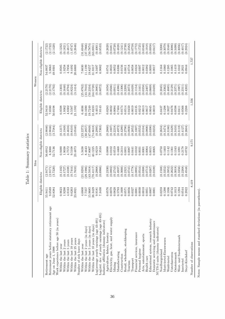
Tab

le1:

Sum

mar

yst

atis

tics

Men

Wom

en

Eligib

led

istr

icts

Non

-eligib

led

istr

icts

Eligib

led

istr

icts

Non

-eligib

led

istr

icts

Ret

irem

ent

age

55.9

411

(2.9

171)

56.6

912

(2.9

046)

52.9

410

(2.2

170)

54.0

937

(2.1

722)

Ret

irem

ent

yea

rsb

efore

statu

tory

reti

rem

ent

age

9.0

589

(2.9

171)

8.3

088

(2.9

046)

7.0

590

(2.2

170)

5.9

063

(2.1

722)

Age

on

Ju

ne

1,

1988

52.8

384

(3.7

220)

52.7

136

(3.7

584)

50.0

198

(2.1

792)

49.9

301

(2.1

420)

Work

exp

erie

nce

bef

ore

age

50

(in

yea

rs)

Wit

hin

the

last

yea

r0.9

623

(0.1

102)

0.9

490

(0.1

217)

0.9

598

(0.1

303)

0.9

585

(0.1

232)

Wit

hin

the

last

2yea

rs1.9

290

(0.1

727)

1.9

038

(0.1

949)

1.9

362

(0.1

640)

1.9

258

(0.1

821)

Wit

hin

the

last

5yea

rs4.8

163

(0.4

108)

4.7

572

(0.4

616)

4.8

302

(0.3

794)

4.7

856

(0.4

817)

Wit

hin

the

last

10

yea

rs9.6

263

(0.7

444)

9.5

108

(0.8

410)

9.5

507

(0.8

224)

9.4

492

(1.0

747)

Wit

hin

the

last

25

yea

rs23.8

921

(1.7

633)

23.4

873

(2.0

540)

21.1

592

(3.1

414)

20.6

869

(3.2

646)

Nu

mb

erof

sick

leave

days

Wit

hin

the

last

yea

r4.6

800

(21.9

293)

5.3

438

(23.2

272)

6.4

036

(25.8

762)

7.6

630

(31.6

948)

Wit

hin

the

last

2yea

rs(i

nd

ays)

7.7

357

(29.1

986)

8.4

643

(30.2

857)

10.1

690

(33.7

910)

11.1

199

(37.7

866)

Wit

hin

the

last

5yea

rs(i

nd

ays)

15.9

685

(43.5

918)

17.8

007

(47.6

949)

19.7

249

(50.2

334)

19.8

257

(50.7

874)

Wit

hin

the

last

10

yea

rs(i

nd

ays)

38.3

429

(70.4

117)

40.1

225

(74.8

618)

31.8

233

(64.5

720)

31.9

317

(63.8

951)

Log(a

ver

age

yea

rly

earn

ings

(age

43-4

9))

9.9

181

(0.2

968)

9.8

219

(0.2

995)

9.4

013

(0.3

885)

9.3

497

(0.4

001)

Log(s

td.

dev

.of

yea

rly

earn

ings

(age

43-4

9))

7.3

430

(0.6

966)

7.3

534

(0.7

363)

7.0

143

(0.8

072)

6.9

082

(0.8

533)

Ind

ust

ryaffi

liati

on

(du

mm

yin

dic

ato

rs)

Agri

cult

ure

,fi

sher

y,fo

rest

ry0.0

576

(0.2

330)

0.0

898

(0.2

860)

0.0

283

(0.1

658)

0.0

741

(0.2

620)

Ele

ctri

city

,gas,

hea

t,an

dw

ate

rsu

pp

ly0.0

078

(0.0

882)

0.0

102

(0.1

007)

0.0

032

(0.0

566)

0.0

023

(0.0

481)

Min

ing

0.0

820

(0.2

743)

0.0

519

(0.2

218)

0.0

084

(0.0

911)

0.0

052

(0.0

720)

Manu

fact

uri

ng

0.5

793

(0.4

937)

0.4

468

(0.4

972)

0.7

404

(0.4

386)

0.6

306

(0.4

828)

Con

stru

ctio

n0.1

600

(0.3

666)

0.2

414

(0.4

280)

0.0

174

(0.1

306)

0.0

156

(0.1

241)

Ret

ail,

wh

ole

sale

,st

ock

kee

pin

g0.0

571

(0.2

321)

0.0

851

(0.2

790)

0.0

514

(0.2

209)

0.0

811

(0.2

730)

Tou

rism

0.0

056

(0.0

745)

0.0

087

(0.0

930)

0.0

450

(0.2

073)

0.0

718

(0.2

582)

Tra

nsp

ort

0.0

327

(0.1

778)

0.0

441

(0.2

052)

0.0

019

(0.0

439)

0.0

058

(0.0

759)

Fin

an

cial

serv

ices

,in

sura

nce

0.0

081

(0.0

895)

0.0

102

(0.1

007)

0.0

135

(0.1

154)

0.0

324

(0.1

772)

Per

son

al

hygie

ne

0.0

030

(0.0

544)

0.0

031

(0.0

552)

0.0

212

(0.1

441)

0.0

307

(0.1

725)

Art

s,en

tert

ain

men

t,sp

ort

s0.0

010

(0.0

308)

0.0

001

(0.0

104)

0.0

013

(0.0

358)

0.0

012

(0.0

340)

Hea

lth

care

0.0

051

(0.0

713)

0.0

064

(0.0

800)

0.0

617

(0.2

407)

0.0

382

(0.1

918)

Ed

uca

tion

al

syst

em,

rese

arc

hin

du

stry

0.0

007

(0.0

267)

0.0

015

(0.0

390)

0.0

045

(0.0

669)

0.0

093

(0.0

958)

Dom

esti

cse

rvic

ing

an

dm

ain

ten

an

ce0.0

001

(0.0

109)

0.0

005

(0.0

233)

0.0

019

(0.0

439)

0.0

017

(0.0

417)

NU

TS

-3u

nit

s(d

um

my

ind

icato

rs)

Nord

bu

rgen

lan

d0.0

259

(0.1

588)

0.0

750

(0.2

634)

0.0

437

(0.2

045)

0.1

164

(0.3

208)

Most

vie

rtel

-Eis

enw

urz

en0.1

290

(0.3

352)

0.1

403

(0.3

474)

0.1

298

(0.3

362)

0.1

060

(0.3

079)

Wald

vie

rtel

0.1

936

(0.3

952)

0.1

142

(0.3

180)

0.3

927

(0.4

885)

0.1

285

(0.3

348)

Unte

rkaer

nte

n0.0

742

(0.2

622)

0.1

361

(0.3

429)

0.0

476

(0.2

129)

0.1

065

(0.3

086)

Ost

stei

erm

ark

0.1

013

(0.3

018)

0.1

343

(0.3

410)

0.0

598

(0.2

371)

0.1

419

(0.3

490)

Wes

t-u

nd

Su

edst

eier

mark

0.1

294

(0.3

356)

0.1

091

(0.3

118)

0.0

411

(0.1

987)

0.1

042

(0.3

056)

Innvie

rtel

0.0

544

(0.2

268)

0.2

178

(0.4

127)

0.0

566

(0.2

311)

0.2

021

(0.4

017)

Ste

yr-

Kir

chd

orf

0.2

922

(0.4

548)

0.0

732

(0.2

604)

0.2

288

(0.4

202)

0.0

944

(0.2

924)

Nu

mb

erof

ob

serv

ati

on

s8,4

19

9,1

71

1,5

56

1,7

27

Note

s:S

am

ple

mea

ns

an

dst

an

dard

dev

iati

on

s(i

np

are

nth

eses

).

36

Tab

le2:

Stan

dard

ized

mor

talit

yra

tes,

1978

-198

4

Men

Wom

en

Age

grou

p<

4545

-65

65-7

5>

75<

4545

-65

65-7

5>

75

Mea

n5.

0557

7.13

558.

3811

9.58

724.

2331

6.34

417.

7217

9.29

52St

anda

rdde

viat

ion

0.14

910.

1222

0.08

560.

0630

0.14

940.

1130

0.09

750.

0828

Elig

ible

dist

rict

0.04

32−

0.04

89−

0.00

450.

0008

−0.

0370

−0.

0427

−0.

0078

0.00

69(0.0

417)

(0.0

318)

(0.0

220)

(0.0

139)

(0.0

543)

(0.0

447)

(0.0

233)

(0.0

215)

Num

ber

ofD

istr

icts

9393

9393

9393

9393

R2

0.01

590.

0303

0.00

050.

0000

0.01

160.

0270

0.00

120.

0013

p-va

lue

(F-s

tati

stic

)0.

3022

0.12

720.

8379

0.95

540.

4968

0.34

170.

7380

0.75

02

Note

s:???,

??,

?den

ote

sst

ati

stic

al

signifi

cance

at

the

1%

,5%

,and

10%

level

resp

ecti

vel

y.R

obust

standard

erro

rsin

pare

nth

eses

.T

he

dep

enden

tva

riable

isth

elo

gof

the

num

ber

of

dec

ease

sp

er100,0

00

resi

den

ts.

All

regre

ssio

ns

are

wei

ghte

dby

dis

tric

ts’

resi

den

tp

opula

tion

in1981.

Sta

ndard

ized

mort

ality

rate

sacc

ount

for

vari

ati

on

inage

dis

trib

uti

on

acr

oss

regio

ns.

Base

don

data

from

Sta

tist

ics

Aust

ria.

37

Tab

le3:

Red

uced

form

effec

ton

sick

leav

eda

ysdu

ring

the

lastk

year

(s)

befo

reag

e50

Men

Wom

en

Sick

leav

eda

ysdu

ring

last

year

last

2ye

ars

last

5ye

ars

last

10ye

ars

last

year

last

2ye

ars

last

5ye

ars

last

10ye

ars

Mea

n5.

0261

8.11

5616.9

238

39.2

707

7.06

6110.6

692

19.7

779

31.8

803

Stan

dard

devi

atio

n22.6

170

29.7

718

45.7

849

72.7

692

29.0

850

35.9

460

50.5

180

64.2

070

Elig

ible

dist

rict

−0.

2817

−0.

0266

−0.

9548

−0.

8047

−1.

4623

−1.

0209

0.07

17−

0.66

94(0.3

335)

(0.4

241)

(0.6

492)

(1.0

382)

(0.9

182)

(1.1

431)

(1.7

162)

(2.2

929)

Coh

ort

fixed

-effe

cts

Yes

Yes

Yes

Yes

Yes

Yes

Yes

Yes

Exp

erie

nce

Yes

Yes

Yes

Yes

Yes

Yes

Yes

Yes

NU

TS-

3fix

ed-e

ffect

sY

esY

esY

esY

esY

esY

esY

esY

esA

ddit

iona

lco

ntro

lsY

esY

esY

esY

esY

esY

esY

esY

es

Num

ber

ofob

serv

atio

ns17,5

9017,5

9017,5

9017,5

903,

283

3,28

33,

283

3,28

3R

20.

2742

0.27

210.

2388

0.25

760.

3655

0.38

000.

3291

0.27

19

Note

s:???,

??,

?den

ote

sst

ati

stic

al

signifi

cance

at

the

1%

,5%

,and

10%

level

resp

ecti

vel

y.R

obust

standard

erro

rsin

pare

nth

eses

.T

her

eare

25

(15)

dis

tinct

male

(fem

ale

)co

hort

s,10

contr

ols

for

past

work

exp

erie

nce

bef

ore

age

50,

and

8dis

tinct

NU

TS-3

regio

ns.

Addit

ional

contr

ol

vari

able

sare

the

log

of

the

aver

age

of

yea

rly

earn

ings

bet

wee

nages

43

and

49,

the

standard

dev

iati

on

of

yea

rly

earn

ings

bet

wee

nages

43

and

49,

and

emplo

yer

s’in

dust

ryaffi

liati

on

(14

indust

ries

).

38

Table 4: First-stage results, men

Retirement years before the statutory retirement age

Mean 8.6678 8.6678 8.6678 8.6678Standard deviation 2.9346 2.9346 2.9346 2.9346

Eligible district 0.7100??? 0.5895???

Eligible district · 1929h2 0.3652?? 0.0900Eligible district · 1930h1 0.1658 −0.0254Eligible district · 1930h2 0.0879 −0.1167Eligible district · 1931h1 0.0307 −0.0617Eligible district · 1931h2 0.7390??? 0.5466???

Eligible district · 1932h1 0.6021??? 0.4285??

Eligible district · 1932h2 0.8066??? 0.6584???

Eligible district · 1933h1 0.6284??? 0.4503??

Eligible district · 1933h2 0.3868? 0.2533Eligible district · 1934h1 0.6323??? 0.4812??

Eligible district · 1934h2 0.9923??? 0.8322???

Eligible district · 1935h1 0.9849??? 0.7802???

Eligible district · 1935h2 0.7494??? 0.5207??

Eligible district · 1936h1 1.2162??? 1.1637???

Eligible district · 1936h2 0.6622??? 0.6336???

Eligible district · 1937h1 1.0500??? 1.0469???

Eligible district · 1937h2 1.3570??? 1.2406???

Eligible district · 1938h1 0.9968??? 0.9708???

Eligible district · 1938h2 0.5397?? 0.3333Eligible district · 1939h1 1.1068??? 0.9968???

Eligible district · 1939h2 0.7041??? 0.5939???

Eligible district · 1940h1 0.8803??? 0.9863???

Eligible district · 1940h2 0.9150??? 0.8897???

Eligible district · 1941h1 0.9651??? 0.9921???

Eligible district · 1941h2 0.6944??? 0.5212??

Cohort fixed-effects Yes Yes Yes YesExperience Yes Yes Yes YesNUTS fixed-effects Yes Yes Yes YesAdditional controls No Yes No Yes

Number of observations 17,590 17,590 17,590 17,590R2 0.1326 0.1980 0.1357 0.2021First Stage F-statistic (Instruments) 243.0828 174.5787 11.9630 10.2984

Notes: ???, ??, ? denotes statistical significance at the 1%, 5%, and 10% level respectively. Robuststandard errors in parentheses. There are 25 (15) distinct male (female) cohorts, 10 controls for pastwork experience before age 50, and 8 distinct NUTS-3 regions. Additional control variables are the logof the average of yearly earnings between ages 43 and 49, the standard deviation of yearly earningsbetween ages 43 and 49, the number of sick-leave days before age 50 (10 terms), and employers’ industryaffiliation (14 industries).

39

Table 5: First stage effect, women

Retirement years before the statutory retirement age

Mean 6.4526 6.4526 6.4526 6.4526Standard deviation 2.2675 2.2675 2.2675 2.2675

Eligible district 1.0104??? 0.9399???

Eligible district · 1934h2 0.6717?? 0.5006?

Eligible district · 1935h1 0.3345 0.3267Eligible district · 1935h2 0.4140 0.2519Eligible district · 1936h1 0.7349?? 0.4873?

Eligible district · 1936h2 0.7092?? 0.6789??

Eligible district · 1937h1 1.1734??? 0.9597???

Eligible district · 1937h2 1.2091??? 1.0138???

Eligible district · 1938h1 1.1244??? 0.9275???

Eligible district · 1938h2 0.9883??? 1.1578???

Eligible district · 1939h1 0.8349??? 0.8560???

Eligible district · 1939h2 1.6288??? 1.6173???

Eligible district · 1940h1 1.1276??? 1.1186???

Eligible district · 1940h2 1.3271??? 1.2925???

Eligible district · 1941h1 1.2916??? 1.3071???

Eligible district · 1941h2 1.1064??? 1.0060???

Cohort fixed-effects Yes Yes Yes YesExperience Yes Yes Yes YesNUTS fixed-effects Yes Yes Yes YesAdditional controls No Yes No Yes

Number of observations 3,283 3,283 3,283 3,283R2 0.1721 0.2489 0.1779 0.2558First Stage F-statistic (Instruments) 153.1078 137.4533 11.9306 11.2351

Notes: ???, ??, ? denotes significance at the 1%, 5%, and 10% level respectively. Robust standard errorsin parentheses. There are 25 (15) distinct male (female) cohorts, 10 controls for past work experiencebefore age 50, and 8 distinct NUTS-3 regions. Additional control variables are the log of the averageof yearly earnings between ages 43 and 49, the standard deviation of yearly earnings between ages 43and 49, the number of sick-leave days before age 50 (10 terms), and employers’ industry affiliation (14industries).

40

Tab

le6:

Seco

ndst

age

resu

lts,

men

Dea

thbe

fore

age

67

OL

S2S

LS

LIM

L

Mea

n0.

1803

0.18

030.

1803

0.18

030.

1803

0.18

030.

1803

0.18

03St

anda

rdde

viat

ion

0.38

450.

3845

0.38

450.

3845

0.38

450.

3845

0.38

450.

3845

Ret

irem

ent

year

sbe

fore

age

650.

0322

???

0.03

24???

0.00

780.

0122

0.01

62??

0.02

42???

0.01

44?

0.02

31??

(0.0

011)

(0.0

011)

(0.0

088)

(0.0

106)

(0.0

078)

(0.0

086)

(0.0

086)

(0.0

096)

Log

(ave

rage

year

lyea

rnin

gs(a

ge43

-49)

)−

0.10

01???

−0.

1003

???

−0.

1001

???

−0.

1001

???

(0.0

138)

(0.0

140)

(0.0

138)

(0.0

138)

Log

(std

.de

v.of

year

lyea

rnin

gs(a

ge43

-49)

)0.

0172

???

0.01

74???

0.01

73???

0.01

73???

(0.0

047)

(0.0

047)

(0.0

047)

(0.0

047)

Coh

ort

fixed

-effe

cts

Yes

Yes

Yes

Yes

Yes

Yes

Yes

Yes

Exp

erie

nce

Yes

Yes

Yes

Yes

Yes

Yes

Yes

Yes

NU

TS

fixed

-effe

cts

Yes

Yes

Yes

Yes

Yes

Yes

Yes

Yes

Add

itio

nal

cont

rols

No

Yes

No

Yes

No

Yes

No

Yes

Num

ber

ofob

serv

atio

ns17

,590

17,5

9017

,590

17,5

9017

,590

17,5

9017

,590

17,5

90R

20.

0686

0.07

440.

0380

0.05

510.

0553

0.07

120.

0522

0.07

03

Note

s:???,

??,

?den

ote

sst

ati

stic

al

signifi

cance

at

the

1%

,5%

,and

10%

level

resp

ecti

vel

y.R

obust

standard

erro

rsin

pare

nth

eses

.T

her

eare

25

(15)

dis

tinct

male

(fem

ale

)co

hort

s,10

contr

ols

for

past

work

exp

erie

nce

bef

ore

age

50,

and

8dis

tinct

NU

TS-3

regio

ns.

Addit

ional

contr

ol

vari

able

sare

the

num

ber

of

sick

-lea

ve

day

sb

efore

age

50

(10

term

s),

and

emplo

yer

s’in

dust

ryaffi

liati

on

(14

indust

ries

).

41

Tab

le7:

Seco

ndst

age

resu

lts,

wom

en

Dea

thbe

fore

age

67

OL

S2S

LS

LIM

L

Mea

n0.

0719

0.07

190.

0719

0.07

190.

0719

0.07

190.

0719

0.07

19St

anda

rdde

viat

ion

0.25

830.

2583

0.25

830.

2583

0.25

830.

2583

0.25

830.

2583

Ret

irem

ent

year

sbe

fore

age

600.

0081

???

0.00

85???

−0.

0051

−0.

0016

−0.

0032

0.00

02−

0.00

38−

0.00

03(0.0

021)

(0.0

023)

(0.0

096)

(0.0

104)

(0.0

089)

(0.0

095)

(0.0

094)

(0.0

099)

Log

(ave

rage

year

lyea

rnin

gs(a

ge43

-49)

)0.

0152

0.02

120.

0202

0.02

05(0.0

146)

(0.0

162)

(0.0

159)

(0.0

160)

Log

(std

.de

v.of

year

lyea

rnin

gs(a

ge43

-49)

)−

0.00

16−

0.00

26−

0.00

24−

0.00

25(0.0

062)

(0.0

062)

(0.0

062)

(0.0

062)

Coh

ort

fixed

-effe

cts

Yes

Yes

Yes

Yes

Yes

Yes

Yes

Yes

Exp

erie

nce

Yes

Yes

Yes

Yes

Yes

Yes

Yes

Yes

NU

TS

fixed

-effe

cts

Yes

Yes

Yes

Yes

Yes

Yes

Yes

Yes

Add

itio

nal

cont

rols

No

Yes

No

Yes

No

Yes

No

Yes

Num

ber

ofob

serv

atio

ns3,

283

3,28

33,

283

3,28

33,

283

3,28

33,

283

3,28

3R

20.

0184

0.02

800.

0069

0.02

190.

0099

0.02

380.

0090

0.02

34

Note

s:???,

??,

?den

ote

sst

ati

stic

al

signifi

cance

at

the

1%

,5%

,and

10%

level

resp

ecti

vel

y.R

obust

standard

erro

rsin

pare

nth

eses

.T

her

eare

25

(15)

dis

tinct

male

(fem

ale

)co

hort

s,10

contr

ols

for

past

work

exp

erie

nce

bef

ore

age

50,

and

8dis

tinct

NU

TS-3

regio

ns.

Addit

ional

contr

ol

vari

able

sare

the

num

ber

of

sick

-lea

ve

day

sb

efore

age

50

(10

term

s),

and

emplo

yer

s’in

dust

ryaffi

liati

on

(14

indust

ries

).

42

Tab

le8:

Cau

seof

deat

h,m

enon

ly

Men

tal

heal

thSe

lf-in

flict

edO

ther

exte

rnal

Car

diov

ascu

lar

Cer

ebro

vasc

ular

Can

cer

Res

pira

tory

inju

ryca

uses

caus

esca

uses

diso

rder

s

Mea

n0.

0113

0.03

280.

0300

0.27

960.

0524

0.37

010.

0529

Stan

dard

devi

atio

n0.

1059

0.17

810.

1706

0.44

880.

2229

0.48

290.

2239

(a)

Red

uced

form

esti

mat

es

Elig

ible

dist

rict

−0.

0020

−0.

0056

0.00

110.

0275

?−

0.00

69−

0.01

11−

0.00

64(0.0

037)

(0.0

064)

(0.0

062)

(0.0

154)

(0.0

080)

(0.0

166)

(0.0

075)

R2

0.01

920.

0109

0.01

020.

0160

0.01

050.

0172

0.01

55

(b)

2SL

Ses

tim

ates

Ret

irem

ent

year

sbe

fore

age

65−

0.00

33−

0.00

910.

0017

0.04

50?

−0.

0113

−0.

0182

−0.

0105

(0.0

060)

(0.0

105)

(0.0

101)

(0.0

259)

(0.0

132)

(0.0

268)

(0.0

124)

R2

0.01

24.

0.00

88.

.0.

0278

.

Coh

ort

fixed

-effe

cts

(bia

nnua

lly)

Yes

Yes

Yes

Yes

Yes

Yes

Yes

Exp

erie

nce

Yes

Yes

Yes

Yes

Yes

Yes

Yes

NU

TS

fixed

-effe

cts

Yes

Yes

Yes

Yes

Yes

Yes

Yes

Num

ber

ofob

serv

atio

ns3,

967

3,96

73,

967

3,96

73,

967

3,96

73,

967

Note

s:???,

??,

?den

ote

sst

ati

stic

al

signifi

cance

at

the

1%

,5%

,and

10%

level

resp

ecti

vel

y.R

obust

standard

erro

rsin

pare

nth

eses

.T

he

sam

ple

isre

stri

cted

toin

div

iduals

who

die

db

efore

Dec

emb

er2008

and

wit

ha

uniq

ue

matc

hin

gb

etw

een

the

ASSD

and

the

cause

sof

dea

thst

ati

stic

sby

Sta

tist

ics

Aust

ria

(see

text

for

det

ails)

.A

mis

sing

R2

den

ote

sa

neg

ati

ve

R-S

quare

d.

43

Tab

le9:

Mai

ndi

agno

sis

for

hosp

ital

adm

issi

on,

men

only

Men

tal

Car

diov

ascu

lar

Cer

ebro

vasc

ular

Can

cer

Res

pira

tory

heal

thdi

seas

edi

sord

ers

diso

rder

s

Mea

n0.

046

0.25

80.

132

0.35

20.

249

Stan

dard

devi

atio

n0.

209

0.43

80.

339

0.47

80.

433

(a)

Red

uced

form

esti

mat

es

Elig

ible

dist

rict

−0.

006

0.06

90.

003

0.00

60.

046

(0.0

26)

(0.0

47)

(0.0

42)

(0.0

54)

(0.0

48)

R2

0.05

40.

082

0.06

20.

053

0.07

2

(b)

2SL

Ses

tim

ates

Ret

irem

ent

year

sbe

fore

age

65−

0.00

70.

085

0.00

30.

007

0.05

7(0.0

33)

(0.0

68)

(0.0

52)

(0.0

67)

(0.0

61)

R2

0.03

40.

045

0.06

30.

049

0.03

8

Coh

ort

fixed

effec

tsY

esY

esY

esY

esY

esE

xper

ienc

eY

esY

esY

esY

esY

esN

UT

S-3

Yes

Yes

Yes

Yes

Yes

Num

ber

ofob

serv

atio

ns52

352

352

352

352

3

Note

s:???,

??,

?den

ote

sst

ati

stic

al

signifi

cance

at

the

1%

,5%

,and

10%

level

resp

ecti

vel

y.R

obust

standard

erro

rsin

pare

nth

eses

.T

he

sam

ple

isre

stri

cted

toin

div

iduals

who

die

db

etw

een

January

1998

and

Dec

emb

er2002

and

who

are

cover

edby

the

hea

lth

insu

rance

data

from

Upp

erA

ust

ria

(see

text

for

det

ails)

.

44

Tab

le10

:R

etir

emen

t(i

n)vo

lunt

arin

ess,

indi

vidu

als

clos

eth

ese

vera

nce-

pay

thre

shol

d

Dea

thbe

fore

67

Win

dow

arou

ndth

resh

old

1to

6m

onth

s1

to12

mon

ths

Bel

owth

resh

old

Abo

veth

resh

old

Bel

owth

resh

old

Abo

veth

resh

old

Mea

n0.

1862

0.18

620.

1811

0.18

110.

1899

0.18

990.

1622

0.16

22St

anda

rdde

viat

ion

0.38

940.

3894

0.38

520.

3852

0.39

230.

3923

0.36

870.

3687

Ret

irem

ent

year

sbe

fore

age

650.

0225

0.03

34?

0.00

510.

0104

0.01

940.

0314

?0.

0117

0.01

90(0.0

181)

(0.0

189)

(0.0

174)

(0.0

182)

(0.0

145)

(0.0

165)

(0.0

127)

(0.0

145)

Coh

ort

fixed

-effe

cts

Yes

Yes

Yes

Yes

Yes

Yes

Yes

Yes

Exp

erie

nce

Yes

Yes

Yes

Yes

Yes

Yes

Yes

Yes

NU

TS-

3fix

ed-e

ffect

sY

esY

esY

esY

esY

esY

esY

esY

esA

ddit

iona

lco

ntro

lsN

oY

esN

oY

esN

oY

esN

oY

es

Num

ber

ofob

serv

atio

ns1,

332

1,33

21,

458

1,45

82,

938

2,93

82,

866

2,86

6R

-Squ

ared

0.08

900.

1176

0.06

140.

1100

0.06

050.

0823

0.05

050.

0779

Note

s:???,

??,

?den

ote

sst

ati

stic

al

signifi

cance

at

the

1%

,5%

,and

10%

level

resp

ecti

vel

y.R

obust

standard

erro

rsin

pare

nth

eses

.T

her

eare

25

(15)

dis

tinct

male

(fem

ale

)co

hort

s,10

contr

ols

for

past

work

exp

erie

nce

bef

ore

age

50,

and

8dis

tinct

NU

TS-3

regio

ns.

Addit

ional

contr

ol

vari

able

sare

the

log

of

the

aver

age

of

yea

rly

earn

ings

bet

wee

nages

43

and

49,

the

standard

dev

iati

on

of

yea

rly

earn

ings

bet

wee

nages

43

and

49,

the

num

ber

of

sick

-lea

ve

day

sb

efore

age

50

(10

term

s),

and

emplo

yer

s’in

dust

ryaffi

liati

on

(14

indust

ries

).

45

Fig

ure

1:E

arlie

stpo

ssib

lew

ithd

raw

alfr

omth

ela

bor

forc

e

Men

:M

en:

5055

5

8

58

5960

65A

ge

Sta

tuto

ry r

etire

men

t ag

eS

tatu

tory

ret

irem

ent

age

Sta

tuto

ry r

etire

men

t ag

eS

tatu

tory

ret

irem

ent

age

Sta

tuto

ry r

etire

men

t ag

e

Sta

tuto

ry r

etire

men

t ag

e w

ith lo

ng-i

nsur

ance

Sta

tuto

ry r

etire

men

t ag

e w

ith lo

ng-i

nsur

ance

Sta

tuto

ry r

etire

men

t ag

e w

ith lo

ng-i

nsur

ance

Sta

tuto

ry r

etire

men

t ag

e w

ith lo

ng-i

nsur

ance

Sta

tuto

ry r

etire

men

t ag

e w

ith lo

ng-i

nsur

ance

Sta

tuto

ry r

etire

men

t ag

e w

ith lo

ng-i

nsur

ance

Sta

tuto

ry r

etire

men

t ag

e w

ith lo

ng-i

nsur

ance

Sta

tuto

ry r

etire

men

t ag

e w

ith lo

ng-i

nsur

ance

dur

atio

nd

urat

ion

Sp

ecia

l inc

ome

sup

por

tS

pec

ial i

ncom

e su

pp

ort

Sp

ecia

l inc

ome

sup

por

tS

pec

ial i

ncom

e su

pp

ort

Sp

ecia

l inc

ome

sup

por

t

Stil

l aliv

e at

age

50

Stil

l aliv

e at

age

50

Stil

l aliv

e at

age

50

Stil

l aliv

e at

age

50

Une

mp

loym

ent

ben

efits

with

/with

out

RE

BP

Une

mp

loym

ent

ben

efits

with

/with

out

RE

BP

Une

mp

loym

ent

ben

efits

with

/with

out

RE

BP

Une

mp

loym

ent

ben

efits

with

/with

out

RE

BP

Une

mp

loym

ent

ben

efits

with

/with

out

RE

BP

Une

mp

loym

ent

ben

efits

with

/with

out

RE

BP

Une

mp

loym

ent

ben

efits

with

/with

out

RE

BP

Une

mp

loym

ent

ben

efits

with

/with

out

RE

BP

Con

tinuo

us w

ork

hist

ory

up t

o th

is p

oint

Con

tinuo

us w

ork

hist

ory

up t

o th

is p

oint

Con

tinuo

us w

ork

hist

ory

up t

o th

is p

oint

Con

tinuo

us w

ork

hist

ory

up t

o th

is p

oint

Con

tinuo

us w

ork

hist

ory

up t

o th

is p

oint

Con

tinuo

us w

ork

hist

ory

up t

o th

is p

oint

Con

tinuo

us w

ork

hist

ory

up t

o th

is p

oint

(780

em

plo

ymen

t w

eeks

in t

he la

st 2

5 ye

ars)

(780

em

plo

ymen

t w

eeks

in t

he la

st 2

5 ye

ars)

(780

em

plo

ymen

t w

eeks

in t

he la

st 2

5 ye

ars)

(780

em

plo

ymen

t w

eeks

in t

he la

st 2

5 ye

ars)

(780

em

plo

ymen

t w

eeks

in t

he la

st 2

5 ye

ars)

(780

em

plo

ymen

t w

eeks

in t

he la

st 2

5 ye

ars)

(780

em

plo

ymen

t w

eeks

in t

he la

st 2

5 ye

ars)

Wom

en:

Wom

en:

50 5

3

54

53

5

4 5

3

54

5560

Age

Sta

tuto

ry r

etire

men

t ag

eS

tatu

tory

ret

irem

ent

age

Sta

tuto

ry r

etire

men

t ag

eS

tatu

tory

ret

irem

ent

age

Sta

tuto

ry r

etire

men

t ag

e

Sta

tuto

ry r

etire

men

t ag

e w

ith lo

ng-i

nsur

ance

dur

atio

n S

tatu

tory

ret

irem

ent

age

with

long

-ins

uran

ce d

urat

ion

Sta

tuto

ry r

etire

men

t ag

e w

ith lo

ng-i

nsur

ance

dur

atio

n S

tatu

tory

ret

irem

ent

age

with

long

-ins

uran

ce d

urat

ion

Sta

tuto

ry r

etire

men

t ag

e w

ith lo

ng-i

nsur

ance

dur

atio

n S

tatu

tory

ret

irem

ent

age

with

long

-ins

uran

ce d

urat

ion

Sta

tuto

ry r

etire

men

t ag

e w

ith lo

ng-i

nsur

ance

dur

atio

n S

tatu

tory

ret

irem

ent

age

with

long

-ins

uran

ce d

urat

ion

Sta

tuto

ry r

etire

men

t ag

e w

ith lo

ng-i

nsur

ance

dur

atio

n S

tatu

tory

ret

irem

ent

age

with

long

-ins

uran

ce d

urat

ion

S

pec

ial i

ncom

e su

pp

ort

S

pec

ial i

ncom

e su

pp

ort

S

pec

ial i

ncom

e su

pp

ort

S

pec

ial i

ncom

e su

pp

ort

S

pec

ial i

ncom

e su

pp

ort

Stil

l aliv

e at

age

50

Stil

l aliv

e at

age

50

Stil

l aliv

e at

age

50

Stil

l aliv

e at

age

50

Une

mp

loym

ent

ben

efits

with

/with

out

RE

BP

Une

mp

loym

ent

ben

efits

with

/with

out

RE

BP

Une

mp

loym

ent

ben

efits

with

/with

out

RE

BP

Une

mp

loym

ent

ben

efits

with

/with

out

RE

BP

Une

mp

loym

ent

ben

efits

with

/with

out

RE

BP

Une

mp

loym

ent

ben

efits

with

/with

out

RE

BP

Une

mp

loym

ent

ben

efits

with

/with

out

RE

BP

Une

mp

loym

ent

ben

efits

with

/with

out

RE

BP

Con

tinuo

us w

ork

hist

ory

up t

o th

is p

oint

Con

tinuo

us w

ork

hist

ory

up t

o th

is p

oint

Con

tinuo

us w

ork

hist

ory

up t

o th

is p

oint

Con

tinuo

us w

ork

hist

ory

up t

o th

is p

oint

Con

tinuo

us w

ork

hist

ory

up t

o th

is p

oint

Con

tinuo

us w

ork

hist

ory

up t

o th

is p

oint

Con

tinuo

us w

ork

hist

ory

up t

o th

is p

oint

(780

em

plo

ymen

t w

eeks

in t

he la

st 2

5 ye

ars)

(780

em

plo

ymen

t w

eeks

in t

he la

st 2

5 ye

ars)

(780

em

plo

ymen

t w

eeks

in t

he la

st 2

5 ye

ars)

(780

em

plo

ymen

t w

eeks

in t

he la

st 2

5 ye

ars)

(780

em

plo

ymen

t w

eeks

in t

he la

st 2

5 ye

ars)

(780

em

plo

ymen

t w

eeks

in t

he la

st 2

5 ye

ars)

(780

em

plo

ymen

t w

eeks

in t

he la

st 2

5 ye

ars)

46

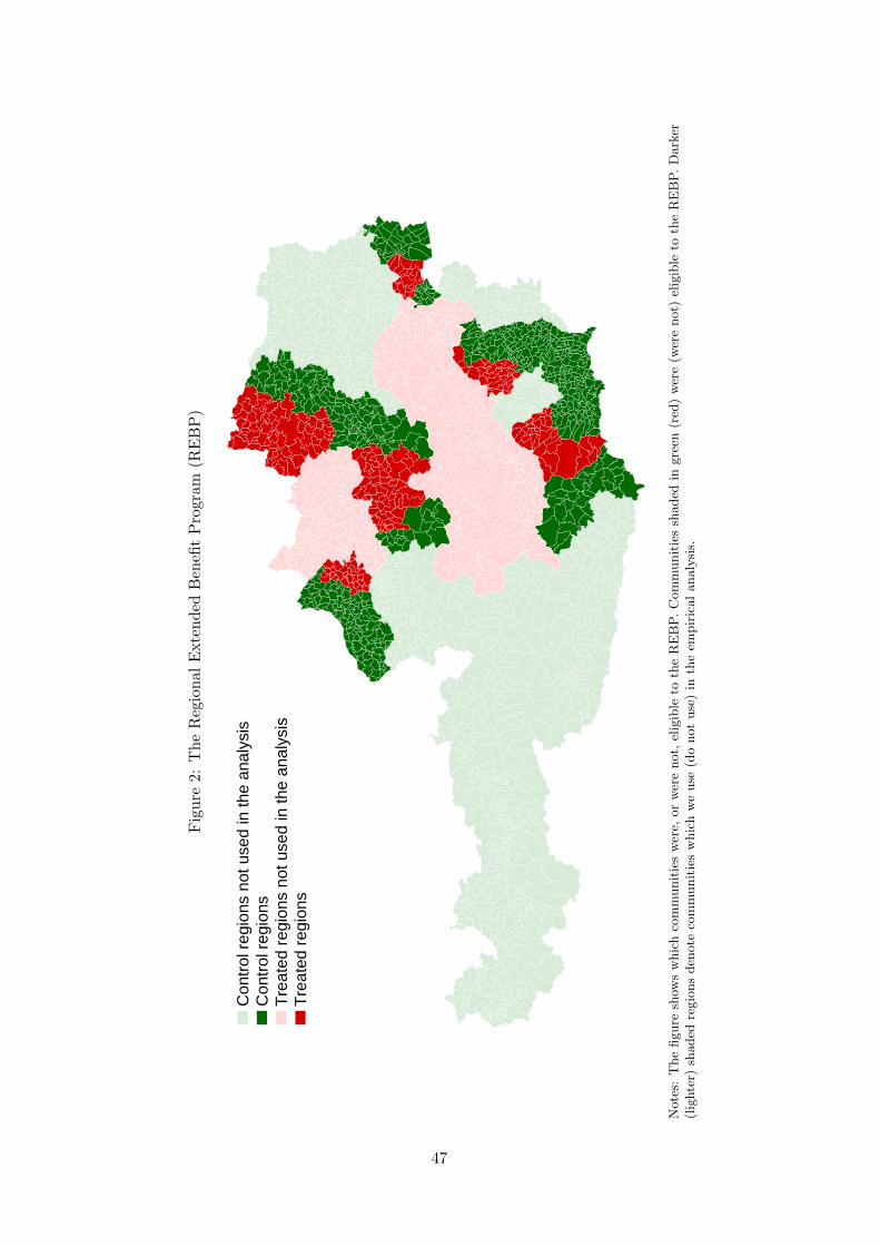
Fig

ure

2:T

heR

egio

nal

Ext

ende

dB

enefi

tP

rogr

am(R

EB

P)

Con

trol

reg

ions

not

use

d in

the

anal

ysis

Con

trol

reg

ions

Tre

ated

reg

ions

not

use

d in

the

anal

ysis

Tre

ated

reg

ions

Note

s:T

he

figure

show

sw

hic

hco

mm

unit

ies

wer

e,or

wer

enot,

elig

ible

toth

eR

EB

P.

Com

munit

ies

shaded

ingre

en(r

ed)

wer

e(w

ere

not)

elig

ible

toth

eR

EB

P.

Dark

er(l

ighte

r)sh

aded

regio

ns

den

ote

com

munit

ies

whic

hw

euse

(do

not

use

)in

the

empir

ical

analy

sis.

47

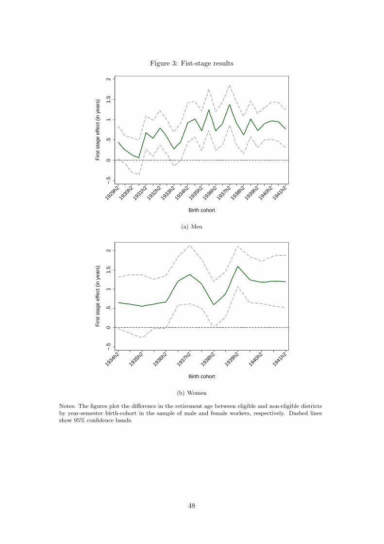
Figure 3: Fist-stage results

−.5

0.5

11.

52

Firs

t sta

ge e

ffect

(in

yea

rs)

1929

h2

1930

h2

1931

h2

1932

h2

1933

h2

1934

h2

1935

h2

1936

h2

1937

h2

1938

h2

1939

h2

1940

h2

1941

h2

Birth cohort

(a) Men

−.5

0.5

11.

52

Firs

t sta

ge e

ffect

(in

yea

rs)

1934

h2

1935

h2

1936

h2

1937

h2

1938

h2

1939

h2

1940

h2

1941

h2

Birth cohort

(b) Women

Notes: The figures plot the difference in the retirement age between eligible and non-eligible districtsby year-semester birth-cohort in the sample of male and female workers, respectively. Dashed linesshow 95% confidence bands.

48

Figure 4: Treatment intensity

−15

−10

−5

0

Diff

eren

ce in

sur

vivo

r fu

nctio

n

50 55 60 65

Retirement age

(a) Men

−25

−20

−15

−10

−5

0

Diff

eren

ce in

sur

vivo

r fu

nctio

n

50 55 60

Retirement age

(b) Women

Notes: The figures show the difference in the survivor function (i.e. the probability of still beingemployed at a given age) between individuals from eligible and non-eligible regions.

49

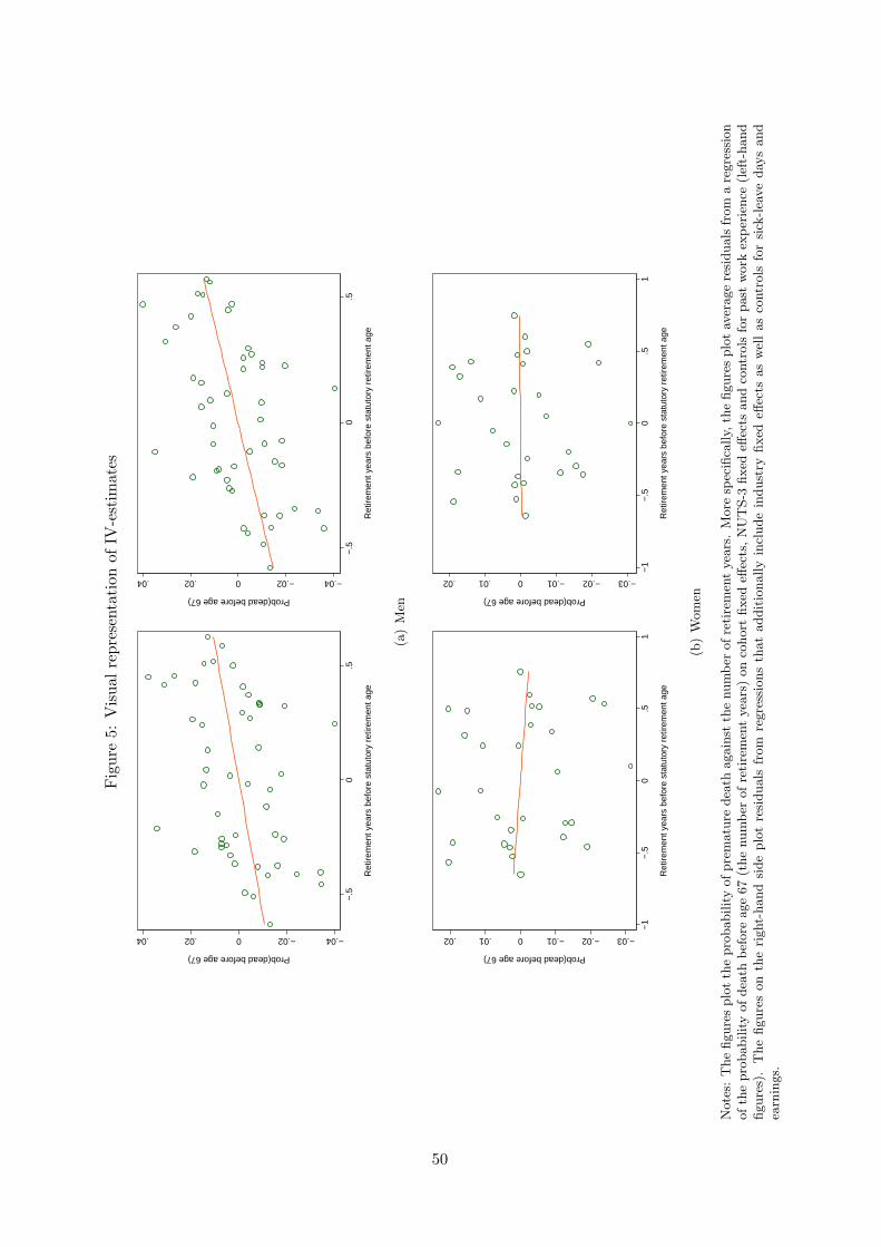
Fig

ure

5:V

isua

lre

pres

enta

tion

ofIV

-est

imat

es

−.04−.020.02.04

Prob(dead before age 67)

−.5

0.5

R

etire

men

t yea

rs b

efor

e st

atut

ory

retir

emen

t age

−.04−.020.02.04

Prob(dead before age 67)

−.5

0.5

R

etire

men

t yea

rs b

efor

e st

atut

ory

retir

emen

t age

(a)

Men

−.03−.02−.010.01.02

Prob(dead before age 67)

−1

−.5

0.5

1

Ret

irem

ent y

ears

bef

ore

stat

utor

y re

tirem

ent a

ge−.03−.02−.010.01.02

Prob(dead before age 67)

−1

−.5

0.5

1

Ret

irem

ent y

ears

bef

ore

stat

utor

y re

tirem

ent a

ge

(b)

Wom

en

Note

s:T

he

figure

splo

tth

epro

babilit

yof

pre

matu

redea

thagain

stth

enum

ber

of

reti

rem

ent

yea

rs.

More

spec

ifica

lly,

the

figure

splo

tav

erage

resi

duals

from

are

gre

ssio

nof

the

pro

babilit

yof

dea

thb

efore

age

67

(the

num

ber

of

reti

rem

ent

yea

rs)

on

cohort

fixed

effec

ts,

NU

TS-3

fixed

effec

tsand

contr

ols

for

past

work

exp

erie

nce

(lef

t-hand

figure

s).

The

figure

son

the

right-

hand

side

plo

tre

siduals

from

regre

ssio

ns

that

addit

ionally

incl

ude

indust

ryfixed

effec

tsas

wel

las

contr

ols

for

sick

-lea

ve

day

sand

earn

ings.

50

A Additional Tables and Figures

Table A.1: First stage results for cohorts ineligible to the REBP

Men Women

Mean 8.2685 5.3875Standard deviation 3.4948 2.1897

Eligible district −0.0071 0.0791(0.1115) (0.0800)

Cohort fixed-effects Yes YesExperience Yes YesNUTS fixed-effects Yes YesAdditional controls Yes Yes

Number of Observations 3, 444 3, 005R2 0.2397 0.1876

Notes: ???, ??, ? denotes statistical significance at the 1%, 5%,and 10% level respectively. Robust standard errors in paren-theses. Considered birth cohorts are 08.1943–04.1947 for menand 08.1943–04.1952 for women. There are 25 (15) distinctmale (female) cohorts, 10 controls for past work experience be-fore age 50, and 8 distinct NUTS-3 regions. Additional controlvariables are the log of the average of yearly earnings betweenages 43 and 49, the standard deviation of yearly earnings be-tween ages 43 and 49, the number of sick-leave days before age50 (10 terms), and employers’ industry affiliation (14 indus-tries).

51

Table A.2: The association between earnings from age 50 onwards and early retirement

Earnings from age 50 onwards

Mean 9.7237 9.7237Standard deviation 0.3540 0.3540

Retirement years before age 65 −0.0222??? −0.0250???

(0.0011) (0.0010)

Cohort fixed-effects Yes YesExperience Yes YesNUTS-3 fixed-effects Yes YesAdditional controls No Yes

Number of observations 17, 590 17, 590R2 0.3141 0.6223

Notes: ???, ??, ? denotes statistical significance at the 1%, 5%, and 10% levelrespectively. Robust standard errors in parentheses. Mean earnings derivedfrom work income, unemployment benefits (assuming a replacement rate of40%), and disability and old-age retirement (assuming a replacement rate of80%) are estimated up to individuals’ death date (right-censored death dates(July 1, 2009) are replaced by the expected death date based on workers’expected life-expectancy (taken from mortality tables by Statistics Austria).There are 25 (15) distinct male (female) cohorts, 10 controls for past workexperience before age 50, and 8 distinct NUTS-3 regions. Additional controlvariables are the log of the average of yearly earnings between ages 43 and 49,the standard deviation of yearly earnings between ages 43 and 49, the numberof sick-leave days before age 50 (10 terms), and employers’ industry affiliation(14 industries).

52

Tab

leA

.3:

Cau

seof

deat

h,m

en(a

ddit

iona

lco

ntro

ls)

Men

tal

heal

thSe

lf-in

flict

edO

ther

exte

rnal

Car

diov

ascu

lar

Cer

ebro

vasc

ular

Can

cer

Res

pira

tory

inju

ryca

uses

diso

rder

s

Mea

n0.

0113

0.03

280.

0300

0.27

960.

0524

0.37

010.

0529

Stan

dard

devi

atio

n0.

1059

0.17

810.

1706

0.44

880.

2229

0.48

290.

2239

(a)

Red

uced

form

esti

mat

es

Elig

ible

dist

rict

−0.

0014

−0.

0047

0.00

240.

0272

?−

0.00

41−

0.01

25−

0.00

83(0.0

037)

(0.0

067)

(0.0

064)

(0.0

158)

(0.0

082)

(0.0

170)

(0.0

079)

R2

0.02

510.

0203

0.01

560.

0225

0.01

690.

0230

0.01

91

(b)

2SL

Ses

tim

ates

Ret

irem

ent

year

sbe

fore

age

65−

0.00

27−

0.00

940.

0048

0.05

43?

−0.

0082

−0.

0250

−0.

0166

(0.0

074)

(0.0

133)

(0.0

126)

(0.0

327)

(0.0

163)

(0.0

334)

(0.0

159)

R2

0.02

11.

0.00

98.

0.00

930.

0310

.

Coh

ort

fixed

-effe

cts

Yes

Yes

Yes

Yes

Yes

Yes

Yes

Exp

erie

nce

Yes

Yes

Yes

Yes

Yes

Yes

Yes

NU

TS

fixed

-effe

cts

Yes

Yes

Yes

Yes

Yes

Yes

Yes

Add

itio

nal

cont

rols

Yes

Yes

Yes

Yes

Yes

Yes

Yes

Num

ber

ofob

serv

atio

ns3,

967

3,96

73,

967

3,96

73,

967

3,96

73,

967

Note

s:???,

??,

?den

ote

ssi

gnifi

cance

at

the

1%

,5%

,and

10%

level

resp

ecti

vel

y.R

obust

standard

erro

rsin

pare

nth

eses

.T

her

eare

25

(15)

dis

tinct

male

(fem

ale

)co

hort

s,10

contr

ols

for

past

work

exp

erie

nce

bef

ore

age

50,

and

8dis

tinct

NU

TS-3

regio

ns.

Addit

ional

contr

ol

vari

able

sare

the

log

of

the

aver

age

of

yea

rly

earn

ings

bet

wee

nages

43

and

49,

the

standard

dev

iati

on

of

yea

rly

earn

ings

bet

wee

nages

43

and

49,

the

num

ber

of

sick

-lea

ve

day

sb

efore

age

50

(10

term

s),

and

emplo

yer

s’in

dust

ryaffi

liati

on

(14

indust

ries

).

53

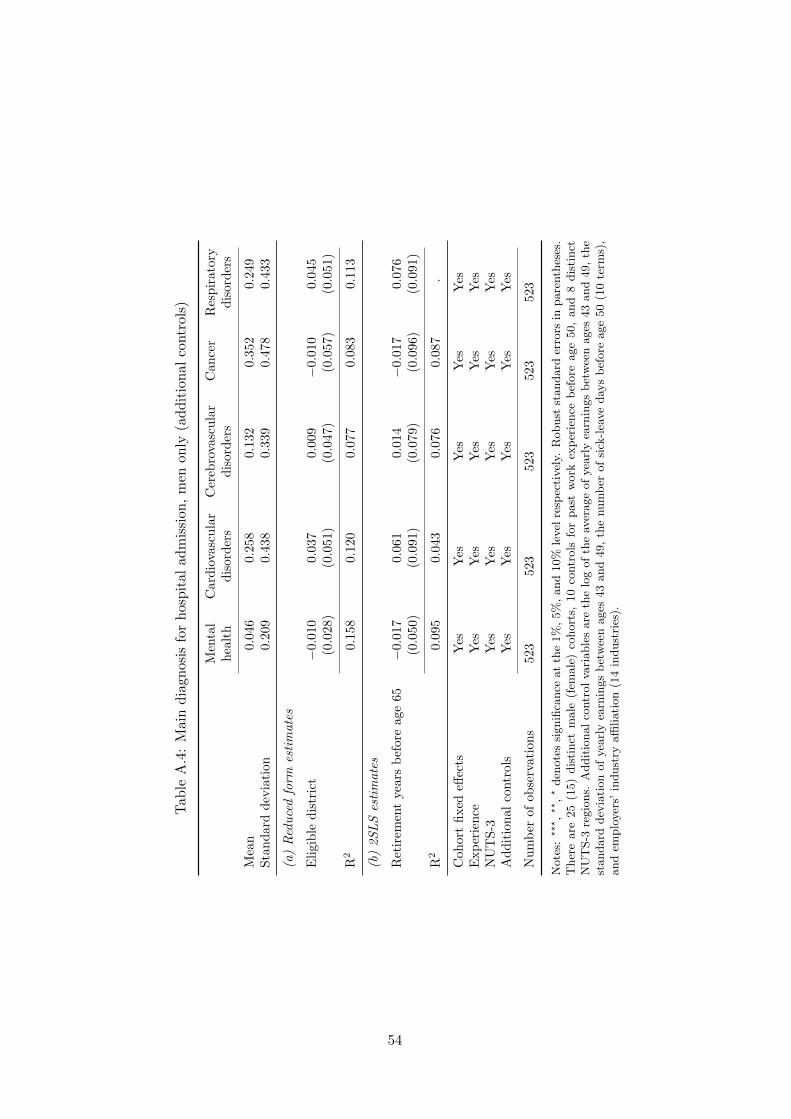
Tab

leA

.4:

Mai

ndi

agno

sis

for

hosp

ital

adm

issi

on,

men

only

(add

itio

nal

cont

rols

)

Men

tal

Car

diov

ascu

lar

Cer

ebro

vasc

ular

Can

cer

Res

pira

tory

heal

thdi

sord

ers

diso

rder

sdi

sord

ers

Mea

n0.

046

0.25

80.

132

0.35

20.

249

Stan

dard

devi

atio

n0.

209

0.43

80.

339

0.47

80.

433

(a)

Red

uced

form

esti

mat

es

Elig

ible

dist

rict

−0.

010

0.03

70.

009

−0.

010

0.04

5(0.0

28)

(0.0

51)

(0.0

47)

(0.0

57)

(0.0

51)

R2

0.15

80.

120

0.07

70.

083

0.11

3

(b)

2SL

Ses

tim

ates

Ret

irem

ent

year

sbe

fore

age

65−

0.01

70.

061

0.01

4−

0.01

70.

076

(0.0

50)

(0.0

91)

(0.0

79)

(0.0

96)

(0.0

91)

R2

0.09

50.

043

0.07

60.

087

.

Coh

ort

fixed

effec

tsY

esY

esY

esY

esY

esE

xper

ienc

eY

esY

esY

esY

esY

esN

UT

S-3

Yes

Yes

Yes

Yes

Yes

Add

itio

nal

cont

rols

Yes

Yes

Yes

Yes

Yes

Num

ber

ofob

serv

atio

ns52

352

352

352

352

3

Note

s:???,

??,

?den

ote

ssi

gnifi

cance

at

the

1%

,5%

,and

10%

level

resp

ecti

vel

y.R

obust

standard

erro

rsin

pare

nth

eses

.T

her

eare

25

(15)

dis

tinct

male

(fem

ale

)co

hort

s,10

contr

ols

for

past

work

exp

erie

nce

bef

ore

age

50,

and

8dis

tinct

NU

TS-3

regio

ns.

Addit

ional

contr

ol

vari

able

sare

the

log

of

the

aver

age

of

yea

rly

earn

ings

bet

wee

nages

43

and

49,

the

standard

dev

iati

on

of

yea

rly

earn

ings

bet

wee

nages

43

and

49,

the

num

ber

of

sick

-lea

ve

day

sb

efore

age

50

(10

term

s),

and

emplo

yer

s’in

dust

ryaffi

liati

on

(14

indust

ries

).

54

Tab

leA

.5:

Hea

lth

pred

ispo

siti

on

Dea

thbe

fore

age

67

Sick

leav

eda

ys(p

ast

10ye

ars)

Bel

owm

edia

nA

bove

med

ian

Mea

n0.

1481

0.14

810.

2117

0.21

17St

anda

rdde

viat

ion

0.35

530.

3553

0.40

850.

4085

Ret

irem

ent

year

sbe

fore

age

650.

0072

0.01

220.

0254

??

0.03

40???

(0.0

110)

(0.0

118)

(0.0

109)

(0.0

120)

Coh

ort

fixed

-effe

cts

Yes

Yes

Yes

Yes

Exp

erie

nce

Yes

Yes

Yes

Yes

NU

TS

fixed

-effe

cts

Yes

Yes

Yes

Yes

Add

itio

nal

cont

rols

No

Yes

No

Yes

Num

ber

ofob

serv

atio

ns8,

681

8,68

18,

909

8,90

9R

20.

0267

0.03

990.

0722

0.08

45

Note

s:???,

??,

?den

ote

sst

ati

stic

al

signifi

cance

at

the

1%

,5%

,and

10%

level

resp

ecti

vel

y.R

obust

standard

erro

rsin

pare

nth

eses

.T

her

eare

25

(15)

dis

tinct

male

(fem

ale

)co

hort

s,10

contr

ols

for

past

work

exp

erie

nce

bef

ore

age

50,

and

8dis

tinct

NU

TS-3

regio

ns.

Addit

ional

contr

ol

vari

able

sare

the

log

of

the

aver

age

of

yea

rly

earn

ings

bet

wee

nages

43

and

49,

the

standard

dev

iati

on

of

yea

rly

earn

ings

bet

wee

nages

43

and

49,

the

num

ber

of

sick

-lea

ve

day

sb

efore

age

50

(10

term

s),

and

emplo

yer

s’in

dust

ryaffi

liati

on

(14

indust

ries

).

55

Fig

ure

A.1

:L

abor

-mar

ket

acti

vity

afte

rag

e50

and

sinc

een

try

into

reti

rem

ent,

resp

ecti

vely

54

32

10

12

3

Diff

eren

ce in

labo

r mar

ket a

ctiv

ities

(in

pp)

out

ofla

bor f

orce

old

age

pens

ion

unem

ploy

ed

empl

oyed

43

21

01

23

4

Diff

eren

ce in

labo

r mar

ket a

ctiv

ities

(in

pp)

out

ofla

bor f

orce

old

age

pens

ion

unem

ploy

ed

(a)

Men

1210

86

42

02

46

8

Diff

eren

ce in

labo

r mar

ket a

ctiv

ities

(in

pp)

out

ofla

bor f

orce

old

age

pens

ion

unem

ploy

ed

empl

oyed

64

20

24

68

D

iffer

ence

in la

bor m

arke

t act

iviti

es (i

n pp

)

out

ofla

bor f

orce

old

age

pens

ion

unem

ploy

ed

(b)

Wom

en

Note

s:T

he

figure

ssh

owdiff

eren

ces

insp

ecifi

cla

bor-

mark

etact

ivit

ies

bet

wee

nel

igib

leand

non-e

ligib

ledis

tric

ts(i

np

erce

nta

ge

poin

ts),

for

men

and

wom

ense

para

tely

.T

he

figure

son

the

left

show

diff

eren

ces

inact

ivit

yfr

om

age

50

unti

lm

in(a

ge

65,

dea

th);

the

figure

son

the

right

show

diff

eren

ces

inact

ivit

yfr

om

the

effec

tive

reti

rem

ent

age

unti

lm

in(a

ge

65,

dea

th).

56