feap - - a finite element analysis programgoico/feap/instalacion/doc/example.pdffeap - - a finite...
TRANSCRIPT

FEAP - - A Finite Element Analysis Program
Version 8.1 Example Manual
Robert L. TaylorDepartment of Civil and Environmental Engineering
University of California at BerkeleyBerkeley, California 94720-1710
E-Mail: [email protected]
January 2007

Contents
1 Introduction 1
2 Example 1. Patch test 2
3 Example 2. Axisymmetric patch test 8
4 Example 2. Truss problem 14
5 Example 3. Circular disk 17
6 Example 4. Strip with hole and slit 29
7 Example 5. Thermal Problem 36
8 Example 6. Coupled Thermo-mechanical 41
9 Example 7. Contact Problem 45
10 Example 8. Finite Deformation Plasticity 49
i

Chapter 1
Introduction
In this manual we provide some examples of problems which can be set up and solvedusing the FEAP program. We begin by describing some of the methods which may beused to define an input data file for some simple finite element analyses. The manualis organized to start with very basic methods for inputs and procedes to more generalmethods to describe input data and problem solutions.
FEAP is controlled using a set of commands. Each command performs a basic step ineither describing a problem or solving a problem. Commands are divided into threebasic groups:
1. Mesh description commands;
2. Problem solution commands; and
3. Graphical display commands.
The appendices of the User Manual contain the optional forms which each input com-mand may have.
It is suggested that new users of FEAP carefully read this manual in its entirity beforestarting to generate their own input datas. The later examples provide ways to managethe data for problems in separate files using an include option. Also, the form of thedata input records may be constructed using parameters to which numerical valuesmay be assigned either in numeric or expression form (see also Chapter 4 of the UserManual).
1
Chapter 2
Example 1. Patch Test.
The first problem considered is a simple patch test in which all the data is specified ex-plicitly. Later examples will illustrate how FEAP can add missing data or use repeatingsimilar parts to generate a mesh.
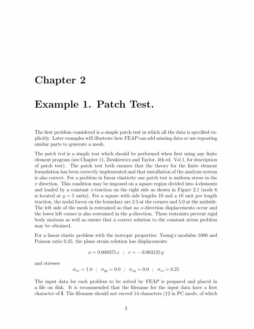
The patch test is a simple test which should be performed when first using any finiteelement program (see Chapter 11, Zienkiewicz and Taylor, 4th ed. Vol 1, for descriptionof patch test). The patch test both ensures that the theory for the finite elementformulation has been correctly implemented and that installation of the analysis systemis also correct. For a problem in linear elasticity one patch test is uniform stress in thex direction. This condition may be imposed on a square region divided into 4-elementsand loaded by a constant x-traction on the right side as shown in Figure 2.1 (node 6is located at y = 5 units). For a square with side lengths 10 and a 10 unit per lengthtraction, the nodal forces on the boundary are 2.5 at the corners and 5.0 at the midside.The left side of the mesh is restrained so that no x-direction displacements occur andthe lower left corner is also restrained in the y-direction. These restraints prevent rigidbody motions as well as ensure that a correct solution to the constant stress problemmay be obtained.
For a linear elastic problem with the isotropic properties: Young’s modulus 1000 andPoisson ratio 0.25, the plane strain solution has displacements
u = 0.009375 x ; v = − 0.003125 y
and stressesσxx = 1.0 ; σyy = 0.0 ; σxy = 0.0 ; σzz = 0.25
The input data for each problem to be solved by FEAP is prepared and placed ina file on disk. It is recommended that the filename for the input data have a firstcharacter of I. The filename should not exceed 14 characters (12 in PC mode, of which
2

CHAPTER 2. EXAMPLE 1. PATCH TEST 3
1 2 3
4
5
6
7 8 9
1 2
3 4
Figure 2.1: Patch Test Mesh
the last 4 may be used for an extender .xxx). When using the program on a PC it isrecommended that no extender be used for the main data input file. Feap uses this filefor generating other files which do contain extenders and, thus, an error could occur.
The filename for the input data of the patch test will be called Ipatch for the discussionbelow. When FEAP is run the names for other files will be assigned by replacing thefirst character (i.e., the I) by one indicating the type of file. For example, the filecontaining the description of the mesh and solution results is called the output fileand for the above choice for the name of the input data file will be named Opatch.The complete input data file for the patch test problem is shown in Table 2.1 and adescription for each part of this data follows.
Input records for FEAP are free format. Each data item is separated by a commaand/or blank characters. If blank characters are used without commas, each data itemmust be included. That is multiple blank fields are not considered to be a zero. Eachdata item is restricted to 14 characters (15 including the blank or comma). Commentsmay be appended to any data record after the character ! (e.g., see Table 2.1).
The input file Ipatch consists of several data sets. For the patch test mesh given inTable 2.1 the data sets are given by the commands (shown without indentation in thetable):
FEAP * * 4-Element Patch TestMATErialCOORdinatesELEMentsBOUNdary restraintsFORCesENDBATCh

CHAPTER 2. EXAMPLE 1. PATCH TEST 4
FEAP * * 4-Element Patch Test9,4,1,2,2,4
MATErial,1SOLId
PLANe STRAinELAStic ISOTropic 1000.0 0.25
! Blank termination recordCOORdinates
1 0 0.0 0.02 0 4.0 0.03 0 10.0 0.04 0 0.0 4.55 0 5.5 5.56 0 10.0 5.07 0 0.0 10.08 0 4.2 10.09 0 10.0 10.0
! Blank termination recordELEMents
1 1 1 1 2 5 42 1 1 2 3 6 53 1 1 4 5 8 74 1 1 5 6 9 8
! Blank termination recordBOUNdary restraints
1 0 1 14 0 1 07 0 1 0
! Blank termination recordFORCes
3 0 2.5 0.06 0 5.0 0.09 0 2.5 0.0
! Blank termination recordEND
Table 2.1: Data for Patch Test
BATChFORM residualTANGentSOLVeDISPlacement ALLSTREss ALL
ENDSTOP
Table 2.2: Data for Patch Test

CHAPTER 2. EXAMPLE 1. PATCH TEST 5
ENDSTOP
FEAP interprets only the first four characters of each command. These are shownas upper case letters to indicate the minimum amount which may be used to identifyeach command. Either upper case or lower case letters may be used to identify eachcommand. Thus, MATE or mate may be used to identify the material propertydata sets. After a FEAP command and the control record, the commands before thefirst END may be in any order and define the mesh for the problem. The commandsafter the BATCH describe the solution algorithm for the problem and terminate withthe second END command. Finally, the STOP command informs FEAP that nomore data exists. Only one problem may appear in the file which contains the probleminitiation command FEAP. See Example 4 in Chapter 6 for a way to run multipleproblems.
The control record defines the size of finite element problem to be solved. The first fielddefines the number of nodes (NUMNP), the next field is the number of elements (NUMEL),followed by the number of material sets (NUMMAT), the spatial dimension for the mesh(NDM), the number of degrees of freedom for each node (NDF), and the maximum numberof nodes on any element (NEN). The patch test has a mesh with 9 nodes, 4 elements,and 1 material set. The problem is 2 dimensional, has 2 degrees of freedom at eachnode, and each element has 4 nodes.
The first data set is identified by the MATErial command. This record also mustcontain a material set number (ranging from 1 to the maximum number of sets needed).The next records consist of commands which describe the type of element (see Chapter6 of the User Manual for the types of elements included with FEAP) and the materialparameters associated with the set. The data shown in Table 2.1 indicates a SOLId(continuum) element is used, the problem is plain strain and the material parametersare associated with a linear elastic isotropic material. Except for the element typerecord, other data may be in any order and terminates with a blank record (commentsare permitted on records and begin with the exclamation point, ”!”).
The values of the nodal coordinates for the patch are specified using the COORdinatecommand. Each record defines a node number, a generation parameter, and the x andy coordinate values. Nodes may be in any order, but are shown in increasing order inTable 2.1. Input terminates with a blank record.
The manner in which nodes are connected to form individual finite elements and theirassociation to the type of element and material parameters is described by the datafollowing the ELEMent command. Each record defines the element number (whichmust be in increasing numerical order), a generation parameter (to be described later),the material data set associated with the element, and the list of nodes connected tothe element. For the elements shown in Figure 2.1 the node sequence must start witha node at one vertex and then proceed with the nodes on vertices traversed counter

CHAPTER 2. EXAMPLE 1. PATCH TEST 6
clockwise around the element. Input terminates with a blank record.
The degree of freedoms for each node may have known applied loads (nodal forces)or may be restrained to satisfy specified nodal displacements. In FEAP all degreeof freedoms are assumed to have specified loading applied unless a restraint code isset. The BOUNdary restraint command may be used to assign restraints to degreeof freedoms which are to have specified displacements. Each record defines a nodenumber, a generation parameter, and the restraint codes for each degree of freedomassociated with the node. A non-zero value for the restraint code indicates that theassociated degree of freedom must satisfy a specified nodal displacement value (defaultis zero); whereas, a zero restraint code indicates the associated degree of freedom has aspecified nodal force (also zero by default). Thus, for the data shown in Table 2.1, node1 has both the u and v displacements restrained; nodes 4 and 7 have the u displacementrestrained and the y force specified. All other nodes have both the x and the y forcesspecified since no restraints are specified. Input terminates with a blank record.
It is evident from the remaining data that no data is provided to impose non-zerodisplacements (methods to input non-zero values are described in Section 5.7 of theUser Manual); however, data is given to impose non-zero forces using the FORCecommand. Each force record defines a node number, a generation parameter, and theforce values for each degree of freedom associated with the node. Thus, for the datagiven in Table 2.1, nodes 3 and 9 have x force values of 2.5 units and node 6 has an xforce value of 5.0 units. Input terminates with a blank record.
The final command after the force values is the END command which terminates inputof the data describing the finite element mesh.
The set of commands shown in Table 2.2 define the solution algorithm to be used in solv-ing the problem. The execution is initiated by the BATCh command (alternatively,it is possible to perform an interactive execution where users enter each command asneeded, see next example and Chapter 11 of the User Manual). The FORM commandinstructs FEAP to form the residual for the equilibrium equations written as:
R(u) = F − P(u)
where F is the vector of applied nodal forces, u is the vector of nodal displacements,and for a static linear elastic problem P is defined as
P = Ku
in which K is the stiffness matrix. A solution to the problem is defined by requiring theresidual to be zero. In FEAP the solution may be computed using Newton’s methodwhich solves a sequence of linear problems. Thus, the TANGent command requeststhe tangent matrix to the residual about the current solution state, u (at start ofexecution the value is zero) where the tangent matrix is defined as:
Ktang = − ∂R
∂u

CHAPTER 2. EXAMPLE 1. PATCH TEST 7
Thus, for a linear elastic static problem the tangent matrix is just K. The SOLVecommand instructs FEAP to solve the incremental (Newton) equations
Ktang ∆u = R
and to update the solution asu ← u + ∆u
For a linear problem this solution sequence should converge in one iteration; thus, theresidual would be zero if the command FORM is given again.
At this point FEAP has computed the solution; however, it is necessary to issueadditional commands to output the values for each type of solution quantity. TheDISPlacement command instructs FEAP to output values for the nodal generalizeddisplacement parameters associated with each nodal degree of freedom (for linear elas-ticity using solid elements these are the values of the u and v displacements at a node).The option ALL requests the displacement values for all active nodes (see manualpages in Appendix A for other options). Similarly, the command STREss, ALL re-quests output values for stresses within all the active elements (see Appendix A forother options). All output is placed in the output file.
Chapter 3
Example 2. Axisymmetric patchtest
A three dimensional solid is described by a body of revolution and is to be analyzedfor the case of axisymmetric behavior. Only small deformations are considered.
For this case the displacement field is given by:
u =
ur(r, z)uz(r, z)
(3.1)
That is, the displacements do not depend on the θ coordinate; however, in FEAP allaxisymmetric problems are formulated for a one radian sector in the θ direction and thefactor 2 π is omitted. The stress and strain for an axisymmetric case may be orderedas:
σ =[σrr σzz σθθ σrz
]T(3.2)
andε =
[εrr εzz εθθ γrz
]T(3.3)
where γij = 2 εij. Using the displacements given by Eq. 3.1 the strain-displacementrelations are given by (Reference: I.S. Sokolnikoff, Mathematical Theory of Elasticity,McGraw-Hill, New York, 1956, pp 182-184.)
ε =
[∂ur
∂r,
∂uz
∂z,
ur
r,
∂ur
∂z+
∂uz
∂r
]T
(3.4)
Similarly, for the above displacement field the equations of equilibrium are given by:
∂σrr
∂r+
∂σrz
∂z+
σrr − σθθ
r+ br = 0
∂σrz
∂r+
σrz
r+
∂σzz
∂z+ bz = 0 (3.5)
8

CHAPTER 3. EXAMPLE 2. AXISYMMETRIC PATCH TEST 9
in which body forces also are axisymmetric and thus are given by b = b(r, z).
For a displacement formulation, a variational problem for linear elasticity may bewritten as
Π(u) =
[ ∫Ω
W (ε) r dr dz −∫
Ω
uT b r dr dz −∫
Γt
uT t r ds
]= min. (3.6)
where W is the stored energy function and ds is a differential length on the two di-mensional r − z boundary. Note also that the factor 2 π is again not included forimplementation into FEAP.
Introducing an isoparametric interpolation for the finite element model as
r = Nα(ξ) rα
z = Nα(ξ) zα
ur = Nα(ξ) uαr
uz = Nα(ξ) uαz
where ξ are natural coordinates, the strain-displacement relations become
ε =
∂Nα
∂r0
0∂Nα
∂zNα
r0
∂Nα
∂z
∂Nα
∂r
uα
r
uαz
uαθ
The variational problem generates the residual equation (again without the factor 2 π)
Rα = Fα −∫
Ω
BTασ r dr dz
in which nodal forces are given by
Fα =
[ ∫Ω
Nαb r dr dz +
∫Γt
Nαt r ds
]Linearizing generates the tangent stiffness used in solution of problems by a Newtonmethod. Accordingly, after the linearization step we obtain
Kαβ =
∫Ω
BTαDT Bβ r dr dz
as the stiffness matrix in which DT is the matrix of tangent moduli for each material.

CHAPTER 3. EXAMPLE 2. AXISYMMETRIC PATCH TEST 10
1 2
3 4
1 2 3
4 5 6
7 8 9
Figure 3.1: (a) 4-node element (b) 9-node element.
The patch test satisfaction requires two parts: A stability test and a consistency test.Here the stability is assessed by computing the eigenvalues for a single element.
An eigenpair assessment is performed for the 4-node element shown in Fig. 1(a). Thecommand language statements needed are:
BATCh
TANG,,-1 ! No factoring performed
EIGE ! Eigenpair for last element
END
and results obtained are:
Eigenvalue
1 2 3 4
1.5094E+04 6.2967E+03 5.9726E+03 4.1488E+03
4.1332E+03 8.7238E+02 1.6841E+02 -4.8317E-13
Eigenvectors
1 2 3 4
2.8467E-01 -1.4779E-01 3.6123E-01 5.7917E-01
2.7360E-01 -3.0785E-01 -3.1771E-01 1.5711E-01
-4.2180E-01 -5.3722E-01 -3.4016E-01 -3.3940E-01
4.0766E-01 3.0785E-01 -3.9098E-01 -1.5711E-01
-4.2180E-01 5.3722E-01 -3.4016E-01 3.3940E-01
-4.0766E-01 3.0785E-01 3.9098E-01 -1.5711E-01
2.8467E-01 1.4779E-01 3.6123E-01 -5.7917E-01
-2.7360E-01 -3.0785E-01 3.1771E-01 1.5711E-01
Eigenvectors

CHAPTER 3. EXAMPLE 2. AXISYMMETRIC PATCH TEST 11
5 6 7 8
2.2696E-02 -5.3662E-01 3.7778E-01 7.8404E-15
-5.6183E-01 -9.2489E-02 -3.6131E-01 5.0000E-01
6.1055E-02 -4.5016E-01 3.1016E-01 6.4563E-15
4.2439E-01 -2.8981E-02 3.6131E-01 5.0000E-01
6.1055E-02 -4.5016E-01 -3.1016E-01 -5.9879E-15
-4.2439E-01 2.8981E-02 3.6131E-01 5.0000E-01
2.2696E-02 -5.3662E-01 -3.7778E-01 -7.1650E-15
5.6183E-01 9.2489E-02 -3.6131E-01 5.0000E-01
The test is repeated for the mesh shown in Fig. 1(b) and the resulting eigenvalues are(vectors are not included here)
Eigenvalue
1 2 3 4
5.1049E+04 4.9787E+04 2.3214E+04 2.0397E+04
1.2530E+04 1.2488E+04 8.1176E+03 7.0663E+03
6.2949E+03 5.8856E+03 4.3601E+03 3.1329E+03
2.3443E+03 2.1822E+03 1.3440E+03 3.6688E+02
9.5560E+01 -6.3612E-12
In both cases there are two rigid body modes : a z-translation and a free rotation in theθ-direction. That is displacements which cause no strain are restricted to
uz = A and uθ = B r
where A and B are constants.
For a part of the consistency test we now consider the test applied to a displacementfield expressed as:
ur = A + B r and uz = 0
we obtain strains
ε =
B
0
A
r+ B
0
and for an isotropic material with constitution
σij = λ εv δij + 2 µ εij

CHAPTER 3. EXAMPLE 2. AXISYMMETRIC PATCH TEST 12
where εv = εij is the volume change in small deformation, the stresses
σ =
λ
(A
r+ 2 B
)+ 2 µ B
λ
(A
r+ 2 B
)λ
(A
r+ 2 B
)+ 2 µ
(A
r+ B
)0
Inserting these stresses into the equilibrium equation requires a non-zero radial bodyforce to be:
br = (λ + 2 µ)A
r2
This body force distribution must be coded into each element to permit the testing ofa patch performance.
1 2 3
45
6
7 8 9
11 2 3 4 5
67 8 9
10
1112 13 14
15
1617 18 19
20
21 22 23 24 25
Figure 3.2: (a) 4-node mesh (b) 9-node mesh.
A rectangular region between 5 ≤ r ≤ 10 and 0 ≤ z ≤ 5 is used (Note that it isimportant not to use a patch which includes a zero radius as no radial displacementis allowed there). The meshes shown in Fig. 2 are use for the patch tests and resultsfor the 9-node mesh are shown in Fig. 3 (results for a4-node element are very similar).Based on the above assessment we find that the element, as coded, passes all the patchtest requirements for stability and consistency.

CHAPTER 3. EXAMPLE 2. AXISYMMETRIC PATCH TEST 13
6.71E+00
7.43E+00
8.14E+00
8.86E+00
9.57E+00
1.03E+01
6.00E+00
1.10E+01
DISPLACEMENT 1
Current ViewMin = 6.00E+00X = 5.00E+00Y = 0.00E+00
Max = 1.10E+01X = 1.00E+01Y = 0.00E+00
Time = 0.00E+00
Figure 3.3: 9-node radial displacement contour.

Chapter 4
Example 2. Truss Problem.
As a next example for the use of FEAP, consider a simple truss problem. The mesh,nodal and element numbers, loading, restraints, and material properties are shown inFigure 4.1.
1 2 3
4 5
1 2
3 4 5 6
7
Figure 4.1: Mesh for Truss Example
The complete data file for the problem is shown in Table 4.1 and a description for eachpart of this data follows.
The control record indicates the mesh has 5 nodes, 7 elements, 2 material sets. It isa 2 dimensional problem with 2 degrees of freedom at each node and 2 nodes for eachtruss element.
The MATEeral property sets for all members are identical except for the cross sectionalarea of the members (the first numerical field on the CROSs SECTion record). Twotypes are indicated: Set 1 has an area of 10 units while set 2 has an area of 5 units.
The coordinates are input as for the patch example described above. Element properties
14

CHAPTER 4. EXAMPLE 2. TRUSS PROBLEM 15
FEAP * * 2-D Truss Problem5 7 2 2 2 2
MATErial,1TRUSS
ELAStic ISOTropic 1000.0CROSs SECTion 10.0
! Blank termination recordMATErial,2
TRUSSELAStic ISOTropic 1000.0CROSs SECTion 5.0
! Blank termination recordCOORdinates
1 0 0.0 0.02 0 200.0 0.03 0 400.0 0.04 0 100.0 160.05 0 300.0 160.0
! Blank termination recordELEMents
1 0 1 1 22 0 1 2 33 0 1 1 44 0 2 2 45 0 2 2 56 0 1 3 57 0 1 4 5
! Blank termination recordBOUNdary restraints
1 0 1 13 0 0 1
! Blank termination recordFORCe
5 0 0.0 -10.0! Blank termination record
ENDINTEractiveSTOP
Table 4.1: Data for Truss Analysis Problem

CHAPTER 4. EXAMPLE 2. TRUSS PROBLEM 16
are also input in a similar way; however, note that the material property set in thethird field now is set to either 1 or 2 depending on whether the cross section has 5 or 10units of area. Boundary restraint conditions are imposed so that node 1 is restrainedto have zero u and v displacements while node 3 has only a restrained v displacement.Finally, a single load in the vertical direction with magnitude -10.0 is applied to node5.
This problem requests an INTEractive mode of solution. In the interactive mode usersmust give the solution commands needed for each solution step. For example, whenthe command FORM is given FEAP will compute the residual and then prompt foranother command input. Similarly, giving the commands for output will display therequest on the screen and also place the information in the output file.

Chapter 5
Example 3. Circular DiskSubjected to Point Loading.
The next problem considered is a circular disk loaded by two concentrated forces of10 units each directed along a diagonal (see Figure 5.1). The material of the disk isassumed to be linearly elastic. Furthermore, for simplicity we consider the loads to beslowly applied so that inertial effects may be ignored. Thus, the model to be solved isa simple linear elastostatics problem. Since the loading is symmetric and we assumethe material to be isotropic (and thus also symmetric), it is only necessary to constructa mesh for one quadrant of the circular disk.
This problem has curved boundaries and requires a general mesh to define the finiteelement solution, thus, more details are described for the input data options availablein FEAP.
Figure 5.1: Circular Disk with Point Loading
In the two dimensional capabilities included in FEAP, the solid elements permit ananalyst to use elements with between 3 and 9 attached nodes. A 3-node element is aplane triangle with nodes located at each vertex. A 4-node element is a quadrilateral
17

CHAPTER 5. EXAMPLE 3. CIRCULAR DISK 18
with nodes at each vertex. A 9-node element is quadrilateral in shape but may havecurved sides defined by nodes located in the mid part of each edge, as well as oneadditional node in the interior. Omitting some midside nodes and/or the center nodeproduces quadrilateral elements with between 5 and 8 nodes.
Let us assume that a mesh will be constructed using 4-node quadrilateral elements.The nodes are defined by a sequence starting with Node 1 and concluding with themaximum number Node NUMNP. The elements also are defined by a sequence startingwith Element 1 and concluding with Element NUMEL. A 4-node quadrilateral elementis defined by the node numbers associated with each vertex. A simple mesh for onequadrant of the disk is shown in Figure 4.1. The figure shows the numbers associatedwith each node and element. This mesh has 19 nodes (NUMNP = 19) and 12 elements(NUMEL = 12).
1 2 3 4 5
67
8
9
10
11
12
13
14
15
16
17
18
19
1 2 3
4
56
7
8
9
10
11
12
Figure 5.2: Finite Element Mesh for Circular Disk with Point Loading
The control data for the mesh shown in Figure 5.2 is:
FEAP * * Example 1. Circular Disk: Basic inputs19 12 1 2 2 4
The remainder of the finite element mesh is described using the data set conceptsintroduced in the previous examples.
There are options to specify the number and coordinates for each nodal point. The oneused to this point is the COORdinate option. Since only the first 4 characters of eachcommand are interpreted by FEAP, the use of COOR or COORDINATE producesidentical results. After the COOR command individual records defining each nodalpoint and its coordinates (in the present case the x1 and x2 coordinates) are specifiedas:

CHAPTER 5. EXAMPLE 3. CIRCULAR DISK 19
N, NG, X-1, X-2
whereN Number of nodal point.NG Generation increment to next node.X-1 value of x-1 coordinate.X-2 value of x-2 coordinate.
Thus, for the mesh shown in Figure 4.1, the coordinate data may be specified as:
COORdinates1 1 0.0000 0.00005 0 1.0000 0.00006 1 0.0000 0.25008 1 0.4500 0.2000
10 0 0.9239 0.382711 1 0.0000 0.500013 1 0.4000 0.400015 0 0.7010 0.701016 0 0.0000 0.750017 0 0.2913 0.686918 0 0.3827 0.923919 0 0.0000 1.0000
! Blank termination record
The missing node numbers and their coordinate values are generated using linear in-terpolation on the NG generation sequence given. Thus, the first pair of records alsogenerates nodes 2 to 4 with coordinates:
2 0.2500 0.00003 0.5000 0.00004 0.7500 0.0000
Comments may be appended after the second character of any line by using an excla-mation followed by the text. Other options to define coordinates are discussed later.
There are also different options which may be used to generate the element connectiondata. One is the ELEMent command which is given as:
N, NG, MA, N-1, N-2, N-3, N-4

CHAPTER 5. EXAMPLE 3. CIRCULAR DISK 20
whereN Number of element.NG Generation increment for node numbers.MA Material identifier associated with element.N-1 Node number for first vertex.N-2 Node number for second vertex.N-3 Node number for third vertex.N-4 Node number for fourth vertex.
Any vertex of the quadrilateral may be used to define N-1. The remainder, however,should be specified using a counter clockwise sequencing around the nodes as shown inFigure 5.3.
1
2
1
2
3
4
Figure 5.3: Node Sequencing for 4-node Quadrilateral
The element connection data for the example problem is given by:
ELEMents1 1 1 1 2 7 65 1 1 6 7 12 119 1 1 11 12 17 16
10 1 1 12 13 14 1711 1 1 14 15 18 1712 0 1 16 17 18 19
! Blank termination record
Elements within a data set must be in order; however, gaps may occur and missingelements will be generated. The second field in each of the element records defines theincrement to apply to nodes in order to generate missing elements. Thus, from the firsttwo pairs of records it is evident that elements 2, 3, and 4 are missing. The generation

CHAPTER 5. EXAMPLE 3. CIRCULAR DISK 21
increment to apply to the nodes on element 2 is specified as 1 on the element 1 record1.Accordingly, the generated elements will have the following sequence of nodes.
2 2 3 8 73 3 4 9 84 4 5 10 9
The material identifier number will be the values specified in the third field and for thedata above will be 1 for all generated elements (the material identifier for generatedelements is taken from the first record of each generation pair).
Multiple ELEMent sets may be used or ELEMent may be combined with otheroptions (e.g., BLOCk type generations).
To complete the problem specification it is necessary to impose constraints on thenodal displacements along the symmetry axes, specify the applied concentrated load,and define the material set properties. A set of commands which accomplish this isgiven by
BOUNdary restraint codes1 1 1 -15 0 0 16 5 -1 0
19 0 1 0! Blank termination record
FORCes on nodes19 0 0 -5.0
! Blank termination record
MATErial,1SOLIdELAStic ISOTropic 10000 0.25 ! E and nuDENSity data 0.1 ! rhoQUADrature data 2 2
! Blank termination recordEND
The set of records following the BOUNdary code command imposes the necessaryrestraints on nodes. A non zero restraint code implies the value of the correspondingdisplacement component will have specified values (default values are 0.0); whereas, azero code (the default restraint code value) indicates the component is unknown andmust be computed. The inputs use generation, similar to the COOR data. Thus the
1If the field is omitted a default value of 1 is assumed.

CHAPTER 5. EXAMPLE 3. CIRCULAR DISK 22
first pair of records will also generate restraints for nodes 2, 3, and 4. A negative orzero code will propagate to the generated node, whereas a positive code will become azero values on the generated nodes. Thus the first pair will generate a set of restraintssuch that the first displacement component (u1) will be an unknown and the secondcomponent (u2) will be set to a specified value. The last pair of records also generatesrestraints for the first degree of freedom of nodes 11 and 16.
For degree of freedoms with zero restraint codes FEAP will add a force value to eachnode (default is 0.0); whereas, for non zero restraint codes FEAP will impose a displace-ment value (default is 0.0). Non zero forces may be specified using a FORCe command(other options also exist as described later). Non zero displacements may be specifiedusing a DISPlacement command (again, other options exist). Thus, for the exampleproblem a concentrated load (F2 = −5) is applied on node 19 by the FORCe commandset shown above. The MATErial record specifies the set number as 1. The next recordrequests the SOLId element type (See Chapters 6 and 7 of the User Manual for ad-ditional information on types of elements and material models permitted). The thirdrecord defines the material constitution as isotropic linear elastic and sets the parame-ters as E = 1000, ν = 0.25. The fourth record sets the material density as ρ = 0.1. Thefifth record specifies a 2× 2 Gauss quadrature to compute arrays and output elementresults. The input of material parameters terminates with a blank record. The datafollowing the SOLId specification may be in any order. Also any data not needed maybe omitted. Since the disk analysis is quasistatic the material density is unnecessaryand could be omitted. Also default quadrature values will be used if this record isomitted. For the current analysis the minimum material data is:
MATErial,1SOLIdELAStic ISOTropic 10000 0.25 ! E and nu
! Blank termination record
The END command signals FEAP that the specification of the mesh and initial loadingconditions is complete. An mesh may be modified during the solution phase by re-entering MESH generation or by manipulating the mesh to merge parts using the TIE
command or setting boundary conditions to satisfy LINK or ELINk conditions.
We next describe some of the other options which are available to generate and/ormanipulate a mesh. Again we consider the example problem to make the discussionspecific.
The preceding format to generate the data for a finite element mesh for the exampleproblem is quite restrictive. If it is desired to increase the number of nodes and elementsit is necessary to restart the process from the very beginning. Thus, we now consideroptions for describing the mesh which permit the problem to be described more easily,as well as, permit the number of nodes and elements to be increased or decreased.

CHAPTER 5. EXAMPLE 3. CIRCULAR DISK 23
FEAP has some powerful options which permit the generation of problems in a formamenable to refinement. For example, the control record pair may be specified with 0nodes, 0 elements, and/or 0 materials indicated. FEAP will use the subsequent data tocompute the number of nodes, elements, and material sets in the mesh2. Accordingly,it is possible to use:
FEAP * * Example 1. Circular Disk: Block inputs0 0 0 2 2 4
Without additional features this is of little merit. However, nodes and elements maybe generated using a BLOCk command as:
PARAmeterm = 2n = 2
! End of parametersBLOCk 1CARTesian,m,n,1,1,1
1 0.0 0.02 0.5 0.03 0.4 0.44 0.0 0.5
! Blank termination record
A BLOCk command uses a regular subdivision of the parent master element shown inFigure 5.2 to describe the mesh within its perimeter. In Figure 5.2 the coordinatedirections 1 and 2 are local axes for the BLOCk generation (i.e., the natural coordinatesfor an isoparametric master element). Using this convention, BLOCk 1 is describedby a 4 node quadrilateral master element whose coordinates are specified as shownabove. The first record states that the master element coordinates will be specified incartesian form (other options are POLAr and SPHErical), the block will be divided intom subdivisions in the 1 direction and n subdivisions in the 2 direction (an m×n meshof quadrilaterals), with the first node, element, and material set numbers set to 1. Thevalues for m and n are assigned prior to the BLOCk specification using the PARAmeter
command followed by the description of parameters. Each parameter may only be onecharacter between a and z (FEAP converts all data to lower case internally, hence only26 parameters are available for use at any one time. Parameters may, however, beredefined at later stages of the data.
Parameters for the sine and cosine of the angles at the middle of the circular part ofblocks are defined by:
PARAmetersp = atan(1.)
2If user mesh functions are employed this feature may not work correctly

CHAPTER 5. EXAMPLE 3. CIRCULAR DISK 24
1
2
1 2
34
5
6
7
8 9
Figure 5.4: Node Sequence to Define Master Nodes on a Block
s = sin(0.5*p)c = cos(0.5*p)
! Blank termination record
Alternatively, the inputs may be specified directly in degrees using the expressions
PARAmeterss = sind(22.5)c = cosd(22.5)
! Blank termination record
Consult Chapter 4 of the User Manual for a list of all functions which may be used inexpressions.
The additional blocks needed to define the circular disk then may be given as:
BLOCk 2CARTesian,n,n
1 0.5 0.02 1.0 0.03 0.701 0.7014 0.4 0.46 c s
! Blank termination record
BLOCk 3CARTesian,n,n
1 0.4 0.4

CHAPTER 5. EXAMPLE 3. CIRCULAR DISK 25
2 0.701 0.7013 0.0 1.04 0.0 0.56 s c
! Blank termination record
The PARAmeter command also permits arithmetic calculations to be performed (seeChapter 4 of the User Manual for further information). In the above, the parameterp is set to 0.25π (i.e., 45 degrees) and s and c are the sin and cosine of 22.5 degrees.The second and third blocks are also 2×2 meshes of quadrilaterals since the value of nhas not been changed; however, each of these blocks are described on an element withone edge curved along the circular boundary of the disk. Note also, that after definingthe initial generation sequence for the node and element numbers on the first block allothers have zero numbers. FEAP will be able to compute the number for the first nodeand element of each block so that the final mesh has 12 elements and 27 nodes (it isnecessary to merge the blocks to produce a mesh with only 19 active nodes needed todefine the problem).
1 2 3
45
6
7
8
9
11 12
14
15
17
1823
24
26
27
1 2
34
5
6
7
89
10
11
12
Figure 5.5: Finite Element Mesh for Circular Disk using Block Commands and Merging
The boundary conditions and applied nodal load may also be defined such that it is notnecessary to know node numbers by using EBOUndary (for edge boundary specification)and CFORced commands (for coordinate point force loading), respectively. Accordingly,
EBOUndary ! Edge boundary restraints1 0.0 1 02 0.0 0 1
! Blank termination recordCFORce ! Coordinate specified forces
NODE 0.0 1.0 0.0 -5.0
CHAPTER 5. EXAMPLE 3. CIRCULAR DISK 26
! Blank termination recordMATErial,1
SOLIdELAStic ISOTropic 10000 0.25DENSity data 0.10QUADrature data 2 2
! Blank termination recordENDTIE ! Tie nodes with same coordinates.
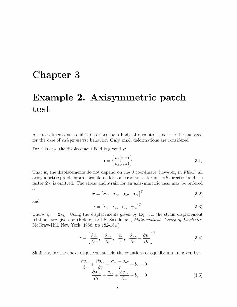
accomplish these steps and complete the description for the mesh and its materialproperties. Note particularly, the TIE command following the generation of the mesh.This command will merge the three blocks to form a mesh which is equivalent to theoriginal mesh (however, this mesh has different numbering for nodes and elementsthan the first mesh generated). The numbers for the active nodes after the merge andthe element numbers produced by the block commands are shown in Figure 5.5. Theadvantage of this form, however, is the ease by which the mesh can be refined. Indeedby assigning the parameter n (and m) a value of 5, one obtains a mesh with 75 elementsas shown in Figure 5.6.
Figure 5.6: Mesh for Circular Disk. 75 Elements
Since the boundary conditions are associated with an edge, all nodes which lie on theedge will be identified and restrained. Similarly, the node with the specified coordinateswill be identified for the applied F2 = −5.0 force. Additional details on options for theCFORce command are given in the mesh user manual pages in Appendix A.
Once the mesh is described the problem may be solved using the solution commandlanguage. Two modes of execution are available: A batch mode where FEAP entersa solution mode and processes all data without user intervention; and an interactive

CHAPTER 5. EXAMPLE 3. CIRCULAR DISK 27
mode where the user issues each command or command group and receives promptsfor additional data. An analysis may use multiple batch and/or interactive solutionsin the same analysis. To enter a batch execution the user inserts a command BATChafter the mesh END record (and any other commands which manipulate the mesh, e.g.,TIE), whereas to enter an interactive mode the command INTEractive is inserted.The BATCh execution command must be immediately followed by the other solutioncommands and terminates with an END command. To perform a batch mode static(steady state) solution for the example problem the commands
BATChTANGent ! Form tangent (K)FORM ! Form residual (R)SOLVe ! Solve K*du = R
END ! End of batch execution
may be included in the input data file after the TIE command. Alternatively, thecommand
INTEractive
may be included and the other commands given sequentially after receiving the
Macro 1.>
prompt. With either mode FEAP process the sequence of commands to produce asolution; however, no report of the results is provided unless specifically requested. Tooutput all the nodal displacement values for the current solution state the command
DISPlacement,ALL
may be given. Similarly, the commands
STREss,ALLREACtion,ALL
produce outputs for all the element variables (stresses and any other values includedin the element output section) and reactions for all the nodes. The order of outputis controlled by the order of issuing the commands. If the solution is converged thennodal reactions should be zero (numerically) for all degree-of-freedoms which are notrestrained. Restrained degree-of-freedoms report the reaction force necessary to imposethe specified displacement constraint.
Alternatively, graphical outputs may be requested. For example, the commands
CHAPTER 5. EXAMPLE 3. CIRCULAR DISK 28
PLOT,MESHPLOT,LOAD,,-1
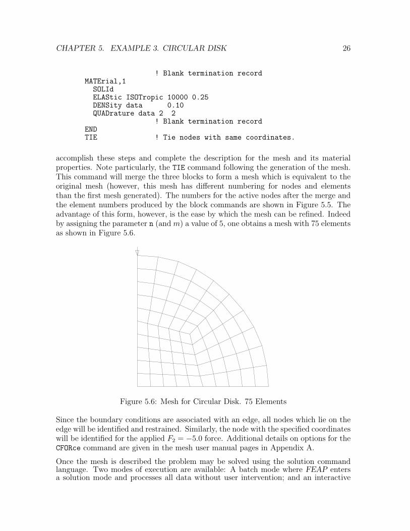
produce the results shown in Figure 5.6. Contour plots are also possible. Shadedcontours for the vertical displacements are shown in Figure 5.7 and are obtained usingthe command
PLOT,CONT,2
Additional information on solution and plot commands is included in Chapters 11 and12 of the User Manual, respectively.
-1.92E-03
-1.60E-03
-1.28E-03
-9.59E-04
-6.39E-04
-3.20E-04
-2.24E-03
3.76E-08
DISPLACEMENT 2
Current ViewMin = -2.24E-03X = 0.00E+00Y = 1.00E+00
Max = 3.76E-08X = 9.87E-01Y = 1.61E-01
Time = 0.00E+00 Time = 0.00E+00
Figure 5.7: Contours of Vertical Displacement for Circular Disk

Chapter 6
Example 4. Strip with Hole andSlit.
As a next example we consider the analysis of a tension strip which contains a holebut has a slit between the hole and the right boundary as shown in Figure 6.1. Thestrip is to be loaded by applying vertical displacements along the top and bottom. Thepossibility of having different materials for the top and bottom halves is anticipatedand, thus, the entire mesh needs to be constructed.
Figure 6.1: Tension Strip with Hole and Slit
To construct the mesh a set of 8 blocks of nodes and elements will be constructedand merged to form the final analysis. Since the mesh has a considerable amountof symmetry it is proposed to generate the two blocks for one quadrant using theBLOCk mesh command and then use the TRANsformation command to form the otherquadrants. The steps to form the mesh may be summarized as follows.
1. Assign REGIon 1 as the first quadrant.
29

CHAPTER 6. EXAMPLE 4. STRIP WITH HOLE AND SLIT 30
2. Use the BLOCk command to form the two blocks for the first quadrant. Save themesh for the first quadrant in a file called IHQUAD.
3. Use an INCLude, IHQUAD in a problem data file (e.g., file ISTRIP) to import thedata for quadrant 1 (see Chapter 4 of the User Manual for more information onuse of the include option.
4. Assign the second and third quadrants to REGIon 2.
5. Set the TRANsformation to reflect the x-axis and use an INCLude, tt IHQUADto generate the 2 blocks for the second quadrant. Note that since the coordi-nate transformation is not a rotation the generated elements may have negativevolume.
6. Set the TRANsformation to reflect the x-axis and y-axes. Use an INCLude, IHQUADto generate the 2 blocks for the third quadrant.
7. Assign the fourth quadrants to REGIon 3.
8. Set the TRANsformation to reflect y-axes. Use an INCLude, IHQUAD to generatethe 2 blocks for the fourth quadrant.
The commands to perform the transformations and read the include files are summa-rized in Figure 6.2.
The outlines for all the blocks formed after this step are shown in Figure 6.3. It isnecessary now to merge these blocks to form the final mesh, while retaining the slit,which if not properly treated will be merged also during the use of a TIE command.
It is at this time that the utility of the REGIon descriptions is used. A summary of themerge order is as follows
1. Merge each of the regions with itself. The result of this step is shown in Figure6.4.
2. Merge region 1 with region 2; also merge region 2 with region 3. This will producethe final mesh whose outline was shown in Figure 6.1.
The TIE commands to achieve these two steps are:
TIE,REGIon,1,1TIE,REGIon,2,2TIE,REGIon,3,3TIE,REGIon,1,2TIE,REGIon,2,3

CHAPTER 6. EXAMPLE 4. STRIP WITH HOLE AND SLIT 31
FEAP * * Tension Strip With Hole and Slit0,0,0,2,2,4PARAmeters
d=1 ! First node numbere=1 ! First element numberm=1 ! Material set numbern=8 ! Size of blocks
! TerminatorREGIon,1 ! Assigns 1st quadrant to region 1
INCLude,IHQUAD ! Input first quadrantPARAmeters
d=0 ! To make feap count nodese=0 ! To make feap count elements
! TerminatorREGIon,2 ! Assign 2nd and 3rd quadrant
TRANsform ! Reverse x axis for second quadrant-1,0,00,1,00,0,10,0,0
INCLude,IHQUADTRANsform ! Reverse x,y axis for third quadrant
-1,0,00,-1,00,0,10,0,0
INCLude,IHQUADREGIon,3 ! Assign 4th quadrant to region 3
TRANsform ! Reverse y axis for fourth quadrant1,0,00,-1,00,0,10,0,0
INCLude,IHQUADEND
Figure 6.2: Region, Transformation, and Include Structure

CHAPTER 6. EXAMPLE 4. STRIP WITH HOLE AND SLIT 32
Figure 6.3: Tension Strip: Block Structure Before Merges
Figure 6.4: Tension Strip: After Merge of Each Region with Itself
The generation of the two blocks forming each quadrant is achieved using the commandsshown in Figure 6.5.
Finally, the displacements on the top and bottom edges are specified using the com-mands given in Figure 6.6.
An analysis using this data produced the results for the σyy stress shown in Figure 6.
Since no explicit use of node element numbers appears in any of the data it is possibleto run a number of problems using the same data but different values for the mesh gen-eration parameter n. Indeed all problems may be performed during the same executionof the program by defining a master input file, say ISLIT which has the values for theparameters. The file ISLIT can contain the data shown in Fig. 6.8. It is necessary toremove the definition of the parameter n from the ISTRIP file. It is further assumedthat the solution commands are also contained in the ISTRIP file or in a file which isreferenced by an include file. Finally, no STOP command should be referenced by theISTRIP file. FEAP will perform all three problems and place the output sequentially

CHAPTER 6. EXAMPLE 4. STRIP WITH HOLE AND SLIT 33
PARAmc=cosd(45.0)s=sind(45.0)a=cosd(22.5)b=sind(22.5)
! TerminationBLOCk
CART,n,n,d,e,m1,1,02,6,03,6,84,s,c5,2.6,07,2.1,2.88,a,b9,2.5,1.2
! TerminationBLOCk
CART,n,n,0,0,m1,s,c2,6,83,0,84,0,15,2.1,2.87,0,3.18,b,a9,1.1,3.0
! Termination
Figure 6.5: Tension Strip with Slit: Block Generation of Quadrant
EBOUndary2 8 0 1 02 -8 0 1 0
! TerminationCBOUndary
node -6 0 1 0! Termination
EDISplacements2 8 0 0.52 -8 0 -0.5
! TerminationMATErial 1
SOLIdELAStic ISOTopic 10000 0.25
! Termination
Figure 6.6: Tension Strip with Slit: Boundary and Material Parameters

CHAPTER 6. EXAMPLE 4. STRIP WITH HOLE AND SLIT 34
S T R E S S 2Min = -1.17E+02Max = 2.32E+03
2.31E+02
5.79E+02
9.26E+02
1.27E+03
1.62E+03
1.97E+03
Current ViewMin = -1.17E+02X = 5.94E+00Y =-7.10E+00
Max = 2.32E+03X =-1.01E+00Y = 4.26E-18
Figure 6.7: Tension Strip with Slit: Contours of σyy
PARAmetern = 4
INCLude ISTRIP
PARAmetern = 8
INCLude ISTRIP
PARAmetern = 16
INCLude ISTRIP
STOP
Figure 6.8: Include data for tension strip refinements

CHAPTER 6. EXAMPLE 4. STRIP WITH HOLE AND SLIT 35
in the file named OSLIT.
The same methodology also may be used to run a sequence of different problems. Inthis case a reference by the include statement would name each of the problem files tobe solved.

Chapter 7
Example 5. Thermal Problem.
In this example we consider the solution of a linear thermal problem. The domain forthe solution is a square with side lengths of 5-units. A steady state and a transientthermal analysis are to be performed. For the steady state analysis a temperature ofT = 1 is applied on the entire left boundary and the right boundary is restrained tohave temperature zero. For the transient problem the left side has a specified unittemperature (T = 1) suddenly applied at time zero and held constant and the rightboundary is insulated (qn = 0). The thermal material parameters are set as follows:
k = 10 c = 1 ρ = 0.1
The problem is solved using a 10× 10 uniform mesh of 9-node quadrilateral elements.For the above properties the material data is specified as:
MATErial 1THERmal
FOURIER ISOTROPIC 10.0 1.0DENSITY MASS 0.10
The mesh is generated using the block command with the data
FEAP0 0 0 2 1 9
BLOCKCARTESIAN 20 20 0 0 1 0 9
1 0.0 0.02 5.0 0.03 5.0 5.04 0.0 5.0
EBOUnd
36

CHAPTER 7. EXAMPLE 5. THERMAL PROBLEM 37
1 0 11 5 1 ! Use for steady state problem only
EDISpl1 0 1
MATE 1... (material properties as above)
END
A plot of the mesh is shown in Fig 7.1
Figure 7.1: Mesh of 9-node elements
The solution to the steady state heat problem is given by:
T (x, y) = 1− x
5
and is exactly captured by the finite element solution as indicated in Fig. 7.2. Thissolution was computed using the commands:
BATChTANGent,,1 ! Solve problemPLOT,CONTour,1 ! Contour solution
END
The transient solution is computed using a transient solution. This may be accom-plished by inserting an ORDEr command after the mesh END command and before thefirst solution execution. The order command is given as

CHAPTER 7. EXAMPLE 5. THERMAL PROBLEM 38
1.43E-01
2.86E-01
4.29E-01
5.71E-01
7.14E-01
8.57E-01
0.00E+00
1.00E+00
DISPLACEMENT 1
Current ViewMin = 0.00E+00X = 5.00E+00Y = 0.00E+00
Max = 1.00E+00X = 0.00E+00Y = 0.00E+00
Time = 0.00E+00
Figure 7.2: Steady state temperature solution (Patch test).
ORDER1
where the 1 restricts transients for the heat equation to a first-order differential equa-tion. Any time integrator could be tried, however, in the results given below the back-ward Euler scheme was used (i.e., TRANsient,BACKward. The solution was performedfor 20 time steps of ∆t = 0.005 with the command language program:
BATCHPARAmeterDT,,dt ! Sets to parameter valueTRANs,BACKLOOP,,20
TIMETANG,,1 ! Problem linear, no iterationsPLOT,RANG,0.4,0.9PLOT,WIPEPLOT,CONT,3 ! Temperature contours
NEXTENDdt= 0.0001
! End of parameter input
A solution at later times is continued using larger time steps. Generally, the solutioncan be computed by increasing the time increment by factors of 10 every logarithmicdecade of time using a FEAP function program. The function program is containedin a file with the extender .fcn. For example a routine for the time increment can begiven by:

CHAPTER 7. EXAMPLE 5. THERMAL PROBLEM 39
dt = 10*dt
stored in the file tinc.fcn. The solution commands are then performed using the setof commands:
BATChDT,,dtLOOP,,4
FUNC,tincLOOP,,9
TIMETANG,,1
NEXTNEXT
END
This will continue the solution to time 10.
Results for the temperature contours at selected times are shown in Figs 7.3 to 7.4.Note that this problem produces one dimensional results and could be solved using amuch simpler meshing.
4.00E-01
5.00E-01
6.00E-01
7.00E-01
8.00E-01
9.00E-01
-3.60E-14
1.00E+00
DISPLACEMENT 1
Current ViewMin = -3.60E-14X = 4.00E+00Y = 5.00E+00
Max = 1.00E+00X = 0.00E+00Y = 0.00E+00
Time = 1.00E-03
4.00E-01
5.00E-01
6.00E-01
7.00E-01
8.00E-01
9.00E-01
2.06E-03
1.00E+00
DISPLACEMENT 1
Current ViewMin = 2.06E-03X = 5.00E+00Y = 5.00E-01
Max = 1.00E+00X = 0.00E+00Y = 0.00E+00
Time = 1.00E-02
Figure 7.3: Temperature contours at t = 0.001 and t = 0.01

CHAPTER 7. EXAMPLE 5. THERMAL PROBLEM 40
4.00E-01
5.00E-01
6.00E-01
7.00E-01
8.00E-01
9.00E-01
5.06E-01
1.00E+00
DISPLACEMENT 1
Current ViewMin = 5.06E-01X = 5.00E+00Y = 5.00E+00
Max = 1.00E+00X = 0.00E+00Y = 0.00E+00
Time = 1.00E-01
4.00E-01
5.00E-01
6.00E-01
7.00E-01
8.00E-01
9.00E-01
9.99E-01
1.00E+00
DISPLACEMENT 1
Current ViewMin = 9.99E-01X = 5.00E+00Y = 4.50E+00
Max = 1.00E+00X = 0.00E+00Y = 0.00E+00
Time = 1.00E+00
Figure 7.4: Temperature contours at t = 0.1 and t = 1.0

Chapter 8
Example 6. CoupledThermo-mechanical Problem.
In this example we consider the solution of a thermo-mechanical problem in a state ofplane strain. The domain for the solution is a square with side lengths of 5-units. Avertical roller support is specified at the upper right-hand corner and a pin support atthe lower right-hand corner. This is just sufficient to prevent rigid body motions for astatic problem. Loading is provided by a transient thermal analysis in which the leftside has a specified unit temperature (T = 1) suddenly applied at time zero and heldconstant. The material parameters are set as follows:
1. Solid:E = 100 ν = 0.4995a α = 0.25 T0 = 0
2. Thermal:k = 10 c = 1 ρ = 0.1
The problem is solved using a 10× 10 uniform mesh of 9-node quadrilateral elements.The mixed formulation is used. With the above properties and element, the materialdata is specified as:
MATErial 1SOLID
ELASTIC ISOTROPIC 100 0.4995THERMAL ISOTROPIC 0.25 0.0FOURIER ISOTROPIC 10.0 1.0DENSITY MASS 0.10MIXED
The mesh is generated using the block command with the data
41

CHAPTER 8. EXAMPLE 6. COUPLED THERMO-MECHANICAL 42
FEAP0 0 0 2 3 9
BLOCKCARTESIAN 20 20 0 0 1 0 9
1 0.0 0.02 5.0 0.03 5.0 5.04 0.0 5.0
CBOUNNODE 5 0 1 1NODE 5 5 1 0
EDIS1 0 0 0 1
MATE 1... (material properties as above)
END
A plot of the mesh is shown in Fig 8.1
Figure 8.1: Mesh of 9-node elements
The solution of the solid mechanics problem is assumed to be at a time scale for whichinertial effects may be ignored. The heat equation, however, is to be solved using atransient solution. This may be accomplished by inserting an ORDEr command afterthe mesh END command and before the first solution execution. The order commandis given as

CHAPTER 8. EXAMPLE 6. COUPLED THERMO-MECHANICAL 43
ORDER0 0 1
where the 0 denotes a zero-order (i.e., static) differential equation form and the 1restricts transients for the heat equation to a first-order differential equation. Anytime integrator could be tried, however, in the results given below the backward Eulerscheme was used (i.e., TRANsient,BACKward. The solution was performed for 20 timesteps of ∆t = 0.005 with the command language program:
BATCHDT,,0.005TRANs,BACKPLOT,DEFOrmPLOT,FACT,0.7 ! to keep plot in windowLOOP,,20
TIMELOOP,,5 ! Note that at least 3 iterations
TANG,,1 ! are needed to converge (since noNEXT ! compling tangent is included)PLOT,WIPEPLOT,RANG,0.4,0.9PLOT,CONT,3 ! Temperature contoursPLOT,RANG,-1.0,0.2PLOT,STRE,1 ! 11-Stress contours
NEXTEND
Results for the contours after the first and last step are shown in Fig 8.2 and 8.3.Numerical results for displacments and temperatures along the row of nodes at x1 =0.25 (center of left row of elemements) are included in Table 8.1
4.00E-01
5.00E-01
6.00E-01
7.00E-01
8.00E-01
9.00E-01
1.70E-03
1.00E+00
DISPLACEMENT 3
Current ViewMin = 1.70E-03X = 4.99E+00Y = 2.50E-01
Max = 1.00E+00X =-6.70E-02Y = 5.64E+00
Time = 5.00E-03Time = 5.00E-03
-1.00E+00
-7.60E-01
-5.20E-01
-2.80E-01
-4.00E-02
2.00E-01
-5.28E+00
1.54E+00
S T R E S S 1
Current ViewMin = -5.28E+00X = 1.59E+00Y = 5.13E+00
Max = 1.54E+00X = 1.89E+00Y = 2.47E+00
Time = 5.00E-03Time = 5.00E-03
Figure 8.2: Thermal stress problem: Time = 0.005
The temperature for the row of nodes shown in the table is constant along the linex1 = 0.25 and equals 0.70261 at time step 1 and 0.96363 at step 20.

CHAPTER 8. EXAMPLE 6. COUPLED THERMO-MECHANICAL 44
4.00E-01
5.00E-01
6.00E-01
7.00E-01
8.00E-01
9.00E-01
5.37E-01
1.00E+00
DISPLACEMENT 3
Current ViewMin = 5.37E-01X = 4.93E+00Y = 3.87E+00
Max = 1.00E+00X =-1.28E+00Y = 6.40E+00
Time = 1.05E-01Time = 1.05E-01
-1.00E+00
-7.60E-01
-5.20E-01
-2.80E-01
-4.00E-02
2.00E-01
-9.98E-01
3.49E-01
S T R E S S 1
Current ViewMin = -9.98E-01X = 2.59E+00Y = 6.07E+00
Max = 3.49E-01X = 1.86E+00Y = 2.98E+00
Time = 1.05E-01Time = 1.05E-01
Figure 8.3: Thermal stress problem: Time = 0.100
Time = 0.005 Time = 0.10Node x2 u1 u2 u1 u2
22 5.00 1.527E-02 5.254E-01 -1.188E+00 1.370E+0023 4.75 -7.526E-02 4.576E-01 -1.216E+00 1.279E+0024 4.50 -1.358E-01 3.921E-01 -1.240E+00 1.189E+0025 4.25 -1.788E-01 3.314E-01 -1.261E+00 1.099E+0026 4.00 -2.101E-01 2.731E-01 -1.278E+00 1.010E+0027 3.75 -2.328E-01 2.180E-01 -1.293E+00 9.207E-0128 3.50 -2.496E-01 1.651E-01 -1.304E+00 8.316E-0129 3.25 -2.614E-01 1.143E-01 -1.313E+00 7.428E-0130 3.00 -2.695E-01 6.483E-02 -1.319E+00 6.543E-0131 2.75 -2.740E-01 1.640E-02 -1.322E+00 5.658E-0132 2.50 -2.756E-01 -3.160E-02 -1.324E+00 4.774E-0133 2.25 -2.740E-01 -7.961E-02 -1.322E+00 3.891E-0134 2.00 -2.695E-01 -1.280E-01 -1.319E+00 3.006E-0135 1.75 -2.614E-01 -1.775E-01 -1.313E+00 2.120E-0136 1.50 -2.496E-01 -2.283E-01 -1.304E+00 1.233E-0137 1.25 -2.328E-01 -2.812E-01 -1.293E+00 3.424E-0238 1.00 -2.101E-01 -3.363E-01 -1.278E+00 -5.505E-0239 0.75 -1.788E-01 -3.947E-01 -1.261E+00 -1.447E-0140 0.50 -1.358E-01 -4.553E-01 -1.240E+00 -2.346E-0141 0.25 -7.526E-02 -5.208E-01 -1.216E+00 -3.248E-0142 0.00 1.527E-02 -5.886E-01 -1.188E+00 -4.151E-01
Table 8.1: Solution for displacements at time step 1 and 20

Chapter 9
Example 7. Contact Problem.
In this example we consider the solution of a two-dimensional contact problem. Twobeams are placed a short distance apart with the top beam loaded by a uniformlydistributed vertical load.
Each beam has a length of 20 units and the spacing between the beams is 0.5 units.The upper beam is divided into 11 equal length elements and the lower beam into 10equal length elements. Each beams is clamped at both ends. Beams are modelled usingthe finite deformation FRAMe element. The material model is elastic (E = 20, 000) witha cross sectional area A = 0.1 and moment of inertia I = 1.
The upper beam is loaded by a uniform load which produces a vertical load of 20× tunits at each node (where t is time). During the analysis t increases from zero to 5 inequal increments of 0.1 units.
The mesh is generated using the commands:
FEAP0 0 0 2 3 2
PARAmeterspr = -20 ! Nodal loadinga = 20 ! Lower beam lengthb = 20 ! Upper beam lengthh = 0.5 ! Spacing between beams
BLOCKCARTesian 10 1 0 0 1
1 0.0 0.02 a 0.0
BLOCKCARTesian 11 1 0 0 2
1 0.0 h
45

CHAPTER 9. EXAMPLE 7. CONTACT PROBLEM 46
2 b h
EBOUnd1 0 1 1 1a 0 1 1 1
EFORce2 h 0 pr
MATE 1FRAMe
ELAStic ISOTropic 20000CROSs section 0.1 1FINIte
MATE 2FRAMe
ELAStic ISOTropic 20000CROSs section 0.1 1FINIte
END
A plot of the mesh is shown in Fig 9.1
Time = 5.00E+00
Figure 9.1: Mesh of two beams
The solution of a contact problem requires the specification of each individual surfaceto be considered and each pair of surfaces for which possible contacts are to be checked.Each surface is defined using a right-hand rule to specify the outward pointing normal.In the present example the contact between the two parallel beams is to be defined. Thelower beam is designated as contact surface number 1 and surface facets are definedfrom the right end to the left end to satisfy the right-hand rule giving a outwardnormal pointing up on the figure. Similarly, the upper beam is designated as contactsurface 2 and facets are numbered from left to right to give an outward normal pointingdown. The two surfaces are specfied to interact using the PAIR command with surface

CHAPTER 9. EXAMPLE 7. CONTACT PROBLEM 47
1 being the slave and surface 2 the master. A node to surface contact with a penaltysolution scheme is adopted (command NTOS) with an augmented lagrange correctionapplied (AUGM). The data for a contact follows the mesh description and for the presentexample is given by:
CONTact
SURFace 1LINE 2FACEt1 -1 11 10
10 0 2 1
SURFace 2LINE 2FACEt1 1 12 13
11 0 22 23
PAIR 1NTOS 1 2SOLM PENAlty 2e3AUGMentTOLE,,1e-5 1e-5 1e-5
END
A solution to the problem is obtained using the commands:
BATChPROPDT,,0.1
END
BATChLOOP,time,50
TIMELOOP,augment,4
LOOP,newton,30TANG,,1
NEXTAUGMent
NEXTNEXT
END
Note especially, the extra loop required to perform the augmentation.
Results for the deformed shape and contours of the final gap achieved (constructedusing the plot command PLOT,CVAR,9, 9= gap) are shown in Fig. 9.2.

CHAPTER 9. EXAMPLE 7. CONTACT PROBLEM 48
Time = 5.00E+00
-2.00E-07
6.00E-07
1.40E-06
2.20E-06
3.00E-06
3.80E-06
-1.00E-06
4.60E-06
CONTACT VAR. 9
Current ViewMin = -1.23E-06X = 1.00E+01Y =-1.68E+00
Max = 9.03E-01X = 0.00E+00Y = 0.00E+00
Time = 5.00E+00
Figure 9.2: Contact deformed shape and gap: Time = 5

Chapter 10
Example 8. Plasticity Problem.
In this example we consider the solution of a plane strain, two-dimensional continuumproblem with an elasto-plastic J2 model. The domain for the problem is a square(with side lengths of 200 mm.) which has a central circular hole (with radius 10 mm.).The top and bottom boundary surfaces are subjected to a uniform normal loading of450 MPa. Due to the symmetry of the problem only one quadrant is modeled andsymmetry boundary conditions are imposed as
u1 = 0 ; on x1 = 0
u2 = 0 ; on x2 = 0
The data for 992 nodes and 900 elements is generated using the commands:
FEAP0 0 0 2 2 4
PARAmetersr = 10h = 100f = 0.4d = 0.35m = 15n = 2*m
SNODes1 0 02 r 03 r*sind(45) r*cosd(45)4 0 r5 h 06 h h7 0 h8 f*h 0
49
CHAPTER 10. EXAMPLE 8. FINITE DEFORMATION PLASTICITY 50
9 0 f*h10 d*h d*h
SIDEpolar 2 3 1polar 3 4 1cart 2 5 8cart 3 6 10cart 4 7 9
BLENdsurf n m 0 0 12 5 6 3
BLENdsurf n m 0 0 13 6 7 4
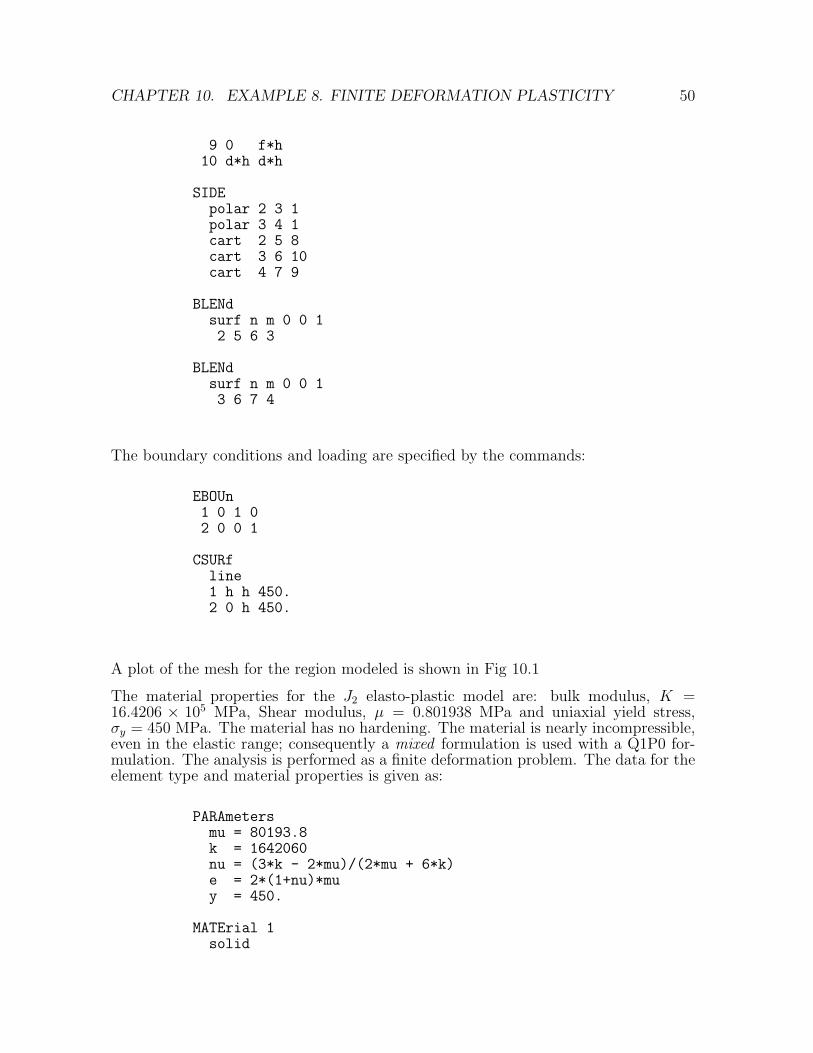
The boundary conditions and loading are specified by the commands:
EBOUn1 0 1 02 0 0 1
CSURfline1 h h 450.2 0 h 450.
A plot of the mesh for the region modeled is shown in Fig 10.1
The material properties for the J2 elasto-plastic model are: bulk modulus, K =16.4206 × 10⁵ MPa, Shear modulus, µ = 0.801938 MPa and uniaxial yield stress,σy = 450 MPa. The material has no hardening. The material is nearly incompressible,even in the elastic range; consequently a mixed formulation is used with a Q1P0 for-mulation. The analysis is performed as a finite deformation problem. The data for theelement type and material properties is given as:
PARAmetersmu = 80193.8k = 1642060nu = (3*k - 2*mu)/(2*mu + 6*k)e = 2*(1+nu)*muy = 450.
MATErial 1solid

CHAPTER 10. EXAMPLE 8. FINITE DEFORMATION PLASTICITY 51
Figure 10.1: Mesh of elasto-plastic tension strip
elastic isotropic e nuplastic mises ymixedfinite
Note that the element requires elastic properties to be given as Young’s modulus and
Poisson ratio (which are computed from the bulk and shear modulus).
Since the mesh consists of two blend regions it is necessary to TIE them together prior
to performing the analysis. The problem is subjected to the cyclic loading shown in
Fig. 10.2 and performed using a sequence of time steps of ∆t = 0.1.

CHAPTER 10. EXAMPLE 8. FINITE DEFORMATION PLASTICITY 52
0 0.5 1 1.5 2 2.5 3 3.5 4−1
−0.8
−0.6
−0.4
−0.2
0
0.2
0.4
0.6
0.8
1
t − Time
p(t)
− L
oad
Figure 10.2: Proportional loading
The command language statements for the analysis are given as:
TIE
BATChPROPDT,,0.1
END2 50 0 1 1 2 0 3 -1 4 0
BATChNOPRintPLOT,RANGe,0,440LOOP,,40
TIMELOOP,,30
TANG,,1NEXTPLOT,PSTRe,6,,1
NEXTEND
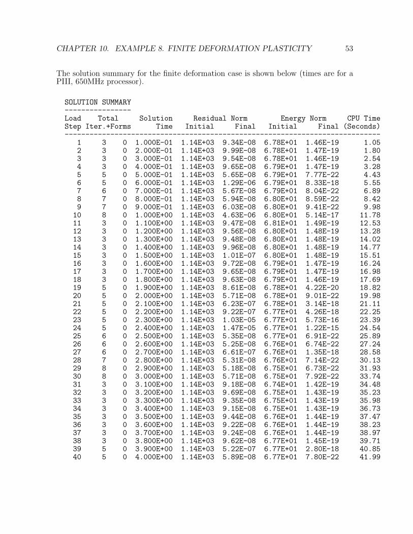
CHAPTER 10. EXAMPLE 8. FINITE DEFORMATION PLASTICITY 53
The solution summary for the finite deformation case is shown below (times are for aPIII, 650MHz processor).
SOLUTION SUMMARY----------------Load Total Solution Residual Norm Energy Norm CPU TimeStep Iter.+Forms Time Initial Final Initial Final (Seconds)----------------------------------------------------------------------------
1 3 0 1.000E-01 1.14E+03 9.34E-08 6.78E+01 1.46E-19 1.052 3 0 2.000E-01 1.14E+03 9.99E-08 6.78E+01 1.47E-19 1.803 3 0 3.000E-01 1.14E+03 9.54E-08 6.78E+01 1.46E-19 2.544 3 0 4.000E-01 1.14E+03 9.65E-08 6.79E+01 1.47E-19 3.285 5 0 5.000E-01 1.14E+03 5.65E-08 6.79E+01 7.77E-22 4.436 5 0 6.000E-01 1.14E+03 1.29E-06 6.79E+01 8.33E-18 5.557 6 0 7.000E-01 1.14E+03 5.67E-08 6.79E+01 8.04E-22 6.898 7 0 8.000E-01 1.14E+03 5.94E-08 6.80E+01 8.59E-22 8.429 7 0 9.000E-01 1.14E+03 6.03E-08 6.80E+01 9.41E-22 9.98
10 8 0 1.000E+00 1.14E+03 4.63E-06 6.80E+01 5.14E-17 11.7811 3 0 1.100E+00 1.14E+03 9.47E-08 6.81E+01 1.49E-19 12.5312 3 0 1.200E+00 1.14E+03 9.56E-08 6.80E+01 1.48E-19 13.2813 3 0 1.300E+00 1.14E+03 9.48E-08 6.80E+01 1.48E-19 14.0214 3 0 1.400E+00 1.14E+03 9.96E-08 6.80E+01 1.48E-19 14.7715 3 0 1.500E+00 1.14E+03 1.01E-07 6.80E+01 1.48E-19 15.5116 3 0 1.600E+00 1.14E+03 9.72E-08 6.79E+01 1.47E-19 16.2417 3 0 1.700E+00 1.14E+03 9.65E-08 6.79E+01 1.47E-19 16.9818 3 0 1.800E+00 1.14E+03 9.63E-08 6.79E+01 1.46E-19 17.6919 5 0 1.900E+00 1.14E+03 8.61E-08 6.78E+01 4.22E-20 18.8220 5 0 2.000E+00 1.14E+03 5.71E-08 6.78E+01 9.01E-22 19.9821 5 0 2.100E+00 1.14E+03 6.23E-07 6.78E+01 3.14E-18 21.1122 5 0 2.200E+00 1.14E+03 9.22E-07 6.77E+01 4.26E-18 22.2523 5 0 2.300E+00 1.14E+03 1.03E-05 6.77E+01 5.73E-16 23.3924 5 0 2.400E+00 1.14E+03 1.47E-05 6.77E+01 1.22E-15 24.5425 6 0 2.500E+00 1.14E+03 5.35E-08 6.77E+01 6.91E-22 25.8926 6 0 2.600E+00 1.14E+03 5.25E-08 6.76E+01 6.74E-22 27.2427 6 0 2.700E+00 1.14E+03 6.61E-07 6.76E+01 1.35E-18 28.5828 7 0 2.800E+00 1.14E+03 5.31E-08 6.76E+01 7.14E-22 30.1329 8 0 2.900E+00 1.14E+03 5.18E-08 6.75E+01 6.73E-22 31.9330 8 0 3.000E+00 1.14E+03 5.71E-08 6.75E+01 7.92E-22 33.7431 3 0 3.100E+00 1.14E+03 9.18E-08 6.74E+01 1.42E-19 34.4832 3 0 3.200E+00 1.14E+03 9.69E-08 6.75E+01 1.43E-19 35.2333 3 0 3.300E+00 1.14E+03 9.35E-08 6.75E+01 1.43E-19 35.9834 3 0 3.400E+00 1.14E+03 9.15E-08 6.75E+01 1.43E-19 36.7335 3 0 3.500E+00 1.14E+03 9.44E-08 6.76E+01 1.44E-19 37.4736 3 0 3.600E+00 1.14E+03 9.22E-08 6.76E+01 1.44E-19 38.2337 3 0 3.700E+00 1.14E+03 9.24E-08 6.76E+01 1.44E-19 38.9738 3 0 3.800E+00 1.14E+03 9.62E-08 6.77E+01 1.45E-19 39.7139 5 0 3.900E+00 1.14E+03 5.22E-07 6.77E+01 2.80E-18 40.8540 5 0 4.000E+00 1.14E+03 5.89E-08 6.77E+01 7.80E-22 41.99

CHAPTER 10. EXAMPLE 8. FINITE DEFORMATION PLASTICITY 54
The solution summary for a small deformation case (remove the FINIte materialrecord) is given below (times are for a PIII, 650MHz processor).
SOLUTION SUMMARY----------------Load Total Solution Residual Norm Energy Norm CPU TimeStep Iter.+Forms Time Initial Final Initial Final (Seconds)----------------------------------------------------------------------------
1 2 0 1.000E-01 1.14E+03 2.12E-10 6.78E+01 7.60E-26 0.592 2 0 2.000E-01 1.14E+03 2.30E-10 6.78E+01 7.82E-26 0.943 2 0 3.000E-01 1.14E+03 2.61E-10 6.78E+01 8.18E-26 1.294 2 0 4.000E-01 1.14E+03 3.06E-10 6.78E+01 8.33E-26 1.655 5 0 5.000E-01 1.14E+03 8.02E-10 6.78E+01 4.47E-24 2.376 5 0 6.000E-01 1.14E+03 1.33E-06 6.78E+01 8.89E-18 3.117 6 0 7.000E-01 1.14E+03 3.52E-10 6.78E+01 3.28E-26 3.988 6 0 8.000E-01 1.14E+03 6.74E-06 6.78E+01 1.93E-16 4.859 7 0 9.000E-01 1.14E+03 3.55E-08 6.78E+01 5.00E-21 5.85
10 8 0 1.000E+00 1.14E+03 4.42E-06 6.78E+01 5.05E-17 6.9911 2 0 1.100E+00 1.14E+03 6.20E-10 6.78E+01 1.44E-25 7.3312 2 0 1.200E+00 1.14E+03 5.43E-10 6.78E+01 1.30E-25 7.6813 2 0 1.300E+00 1.14E+03 5.11E-10 6.78E+01 1.19E-25 8.0114 2 0 1.400E+00 1.14E+03 4.68E-10 6.78E+01 1.10E-25 8.3315 2 0 1.500E+00 1.14E+03 4.22E-10 6.78E+01 1.03E-25 8.6616 2 0 1.600E+00 1.14E+03 3.83E-10 6.78E+01 9.56E-26 9.0117 2 0 1.700E+00 1.14E+03 3.28E-10 6.78E+01 9.13E-26 9.3618 2 0 1.800E+00 1.14E+03 3.03E-10 6.78E+01 8.60E-26 9.6919 5 0 1.900E+00 1.14E+03 1.59E-07 6.78E+01 2.68E-19 10.4420 5 0 2.000E+00 1.14E+03 3.74E-09 6.78E+01 1.22E-22 11.1821 5 0 2.100E+00 1.14E+03 3.03E-07 6.78E+01 6.33E-19 11.9222 6 0 2.200E+00 1.14E+03 9.99E-11 6.78E+01 4.05E-27 12.8223 5 0 2.300E+00 1.14E+03 9.51E-06 6.78E+01 4.81E-16 13.5624 5 0 2.400E+00 1.14E+03 1.34E-05 6.78E+01 9.86E-16 14.3025 6 0 2.500E+00 1.14E+03 2.09E-10 6.78E+01 9.33E-27 15.1926 6 0 2.600E+00 1.14E+03 2.03E-09 6.78E+01 3.26E-23 16.0627 6 0 2.700E+00 1.14E+03 1.77E-07 6.78E+01 1.00E-19 16.9528 7 0 2.800E+00 1.14E+03 5.59E-05 6.78E+01 4.75E-15 17.9629 8 0 2.900E+00 1.14E+03 4.20E-09 6.78E+01 5.83E-23 19.0930 8 0 3.000E+00 1.14E+03 1.32E-09 6.78E+01 6.17E-24 20.2531 2 0 3.100E+00 1.14E+03 5.87E-10 6.78E+01 1.43E-25 20.5632 2 0 3.200E+00 1.14E+03 4.95E-10 6.78E+01 1.18E-25 20.8933 2 0 3.300E+00 1.14E+03 4.80E-10 6.78E+01 1.20E-25 21.2334 2 0 3.400E+00 1.14E+03 4.34E-10 6.78E+01 1.03E-25 21.5635 2 0 3.500E+00 1.14E+03 3.80E-10 6.78E+01 9.84E-26 21.8936 2 0 3.600E+00 1.14E+03 3.54E-10 6.78E+01 9.45E-26 22.2337 2 0 3.700E+00 1.14E+03 3.24E-10 6.78E+01 9.00E-26 22.5438 2 0 3.800E+00 1.14E+03 3.07E-10 6.78E+01 8.64E-26 22.8839 5 0 3.900E+00 1.14E+03 1.79E-07 6.78E+01 3.41E-19 23.6040 5 0 4.000E+00 1.14E+03 1.08E-09 6.78E+01 6.14E-24 24.34
Note that linear elasticity requires only 2 iterations during elastic behavior.