The text that follows is a TRANSLATION O texto que segue é uma TRADUÇÃO Please cite the original article: Favor citar o trabalho original:

Fearnside, P.M. 2009. As hidrelétricas de Belo Monte e Altamira (Babaquara) como fontes de gases de efeito estufa. Novos Cadernos NAEA 12(2): 5-56. Available at: Disponível em: http://www.periodicos.ufpa.br/index.php/ncn/article/view/315/501 English version: Hydroelectric dams planned on Brazil’s Xingu River as sources of greenhouse gases: Belo Monte (Kararaô) and Altamira (Babaquara). (manuscript). [available at: http://philip.inpa.gov.br/publ_livres/mss%20and%20in%20press/Belo%20Monte%20emissions-Engl.pdf

1

Hydroelectric Dams Planned on Brazil’s Xingu River as sources of Greenhouse Gases: Belo Monte (Kararaô) and Altamira (Babaquara)

Philip M. Fearnside1

(1) National Institute for Research in the Amazon (INPA) , C.P. 478, 69011-970 Manaus-Amazonas, Brazil English translation of: Fearnside, P.M. 2009. As hidrelétricas de Belo Monte e Altamira (Babaquara) como fontes de

gases de efeito estufa. Novos Cadernos NAEA 12(2): 5-56. Available at: http://philip.inpa.gov.br/publ_livres/ 2009/Belo%20Monte%20e%20Babaquara%20emissoes-Novos%20Cad%20NAEA.pdf And at: http://www.periodicos.ufpa.br/index.php/ncn/article/view/315/501

Please cite the original article.

Abstract Estimating the greenhouse-gas emissions from hydroelectric dams is important as an input to the decision-making process on public investments in the various options for electricity generation and conservation. Brazil’s proposed Belo Monte Dam (formerly Kararaô) and its upstream counterpart, the Altamira Dam (better known by its former name: Babaquara) are at the center of controversies regarding how greenhouse-gas emissions from dams should be counted. The Belo Monte Dam by itself would have a small reservoir area (440 km2) and large installed capacity (11,181.3 MW), but the Babaquara Dam that would regulate the flow of the Xingu River (thereby increasing power generation at Belo Monte) would flood a vast area (6140 km2). The water level in Babaquara would rise and fall by 23 m each year, annually exposing a drawdown area of 3580 km2 on which soft easily decomposed vegetation would quickly grow. This vegetation would decompose each year at the bottom of the reservoir when the water level rises, producing methane. The methane from drawdown-zone vegetation represents a permanent source of this greenhouse gas, unlike the large peak of emission from decomposition of initial stocks of carbon in the soil and in the leaves and litter of the original forest. The turbines and spillways draw water from below the reservoir’s thermocline, releasing a large part of the dissolved methane to the atmosphere. Carbon dioxide from decay of the above-water portions of trees in the forest that is flooded represents another significant greenhouse gas emission source in the early years after reservoir formation. Belo Monte and Babaquara represent a challenge to Brazil’s

2

fledgling environmental impact assessment and licensing system because the current procedure considers only one infrastructure project at a time, rather than the full range of impacts that the overall development entails. In this case, the unusually favorable characteristics of the first dam (Belo Monte) are highly misleading as indications of the environmental consequences of a decision to build that dam: the principal impacts are in the impetus it gives to creating much larger upstream reservoirs, beginning with Babaquara and possibly including an additional four dams planned for the Xingu Basin, all of which flood tropical rainforest and indigenous land in addition to emitting greenhouse gases. The present analysis indicates that the Belo Monte/Babaquara complex would not break even in terms of greenhouse gas emissions until 41 years after the first dam is filled in a calculation with no discounting, and that any annual discount rate above 1.5% results in the complex failing to perform as well as natural gas by the end of the 50-year time horizon used in Brazil’s assessments of proposed energy projects. The global-warming impact of dams is one indication of the need for Brazil to reassess its current policies that allocate large amounts of energy in the country’s national grid for aluminum smelting for a subsidized export industry. Amazonia – Brazil – Global warming - Greenhouse-gas emissions - Hydroelectric dams - Methane - Reservoirs

The proposed Belo Monte Dam, on Brazil’s Xingu River (a north-flowing tributary to the Amazon in the State of Pará) is the focus of intense controversy due to the magnitude and nature of its impacts. Belo Monte’s impact on global warming stems from the upstream dams that would add substantially to Belo Monte’s electrical output by regulating the flow of the highly seasonal Xingu River. The Belo Monte reservoir itself is small relative to the capacity of its two powerhouses, but the five upstream reservoirs are vast, even by Amazonian standards. The largest of these is the Babaquara Dam--recently re-named the “Altamira Dam” in an apparent effort to escape the onus of the criticism that the plans for Babaquara have attracted over the past two decades (the initial survey, or inventário, began in October 1975). ELETRONORTE (the government power authority in northern Brazil) first proposed the Kararaô Dam (now called “Belo Monte”) with power generation calculations that assumed upstream regulation of streamflow by at least one dam (Babaquara)(CNEC 1980). The series of dams on the Xingu River would have serious consequences for indigenous peoples and for the large areas of tropical rainforest that the reservoirs would flood (e.g., Santos and de Andrade 1990, Sevá and Switkes forthcoming). Difficulties in obtaining environmental approval led to formulation of a second plan for Belo Monte, with calculations that assumed no upstream regulation of streamflow (Brazil, ELETRONORTE 2002). The viability study for the second plan makes clear that the need for an analysis under the assumption of unregulated streamflow stems from “a new economic and socio-environmental perspective” (i.e., from political considerations), and that Belo Monte’s power output would be greater if upstream dams were included in the analysis (Brazil, ELETRONORTE 2002, p. 6-82). Further difficulties in obtaining environmental approval have led ELETRONORTE to initiate a third analysis (still in progress) with several possible smaller installed capacities: 5500, 5900 and 7500 MW (Pinto 2003). These developments in no way imply that a decision has been made not to build the Babaquara (Altamira) Dam upstream of Belo Monte. On the contrary, preparations for construction of Babaquara

3

(Altamira) are included under the current Decennial Plan for the electrical sector (Brazil, MME-CCPESE 2002) and plans for the dam are presented by ELETRONORTE as progressing normally towards construction (Santos 2004). In other words, the one-dam scenario portrayed in the Belo Monte viability study (Brazil, ELETRONORTE 2002) and environmental impact study (Brazil, ELETRONORTE nd [C. 2002]a) appears to represent a bureaucratic fiction that was drafted for the purpose of gaining environmental approval for Belo Monte. The scenario used in the present paper therefore appears most likely as a representation of the overall impact of the development, with the Belo Monte Dam being built according to the 2002 viability study (Brazil, ELETRONORTE 2002), followed by Babaquara (Altamira) in accord with earlier plans (Brazil, ELETRONORTE nd [C. 1988]). Belo Monte cannot be considered alone without taking into account the impacts of upstream dams, particularly Babaquara (Altamira). Among the many impacts of the upstream dams that must be assessed, one is the role they would play in creating greenhouse-gas emissions. In the present analysis, preliminary estimates will be presented for emissions from Belo Monte and Babaquara; if the remaining four planned dams were built, they would have additional impacts. Hydroelectric Dams and Greenhouse-Gas Emissions Belo Monte is at the heart of ongoing controversies regarding the magnitude of the global-warming impact of hydroelectric dams and the proper way that this impact should be quantified and considered in the decision-making process. When the first calculations of greenhouse-gas emissions from the existing dams in Brazilian Amazonia indicated substantial impact (Fearnside 1995a), these conclusions were attacked by presenting a hypothetical case that corresponded to Belo Monte with a power density of over 10 Watts of installed capacity per m2 of reservoir surface area (Rosa and others 1996). In addition to methodological issues that make these hypothetical calculations underestimates of greenhouse-gas impact, the main problem is the omission of the emissions from the 6140-km2 Babaquara Dam upstream of Belo Monte (Fearnside 1996a). This same basic problem remains today, even after many advances in greenhouse-gas emissions estimates. The relatively small area of the Belo Monte Dam by itself means that greenhouse-gas emissions from the reservoir surface will be modest, and when these are divided by the Dam’s 11,181 MW installed capacity the emission appears to be low relative to the benefits. This is the rationale of using the “power density” (Watts of installed capacity per square meter of water area) as the measure of a dam’s global-warming impact. In presenting Belo Monte as an ideal dam from a global-warming perspective, Luis Pinguelli Rosa and coworkers (1996) calculated this ratio as slightly exceeding 10 W/m2, considering the originally planned reservoir area of 1225 km2 (the index would be 25 W/m2 under the same assumptions considering the currently planned 440 km2 area). The regulations of the Kyoto Protocol’s Clean Development Mechanism (CDM) currently allow carbon credit for large dams without restriction, but the Executive Board of the CDM, at its meeting in Buenos Aires in December 2004, proposed that these credits be restricted to dams with power densities of at least 10 W/m2 of reservoir area (UN-FCCC 2004, p. 4), coincidentally the mark achieved by Belo Monte as calculated by Rosa and others (1996). The possibility of claiming carbon credit for Belo Monte

4

has been raised on several occasions both by Brazilian and World Bank officials (personal observation). A power density as high as 10 W/m2 for Belo Monte requires that this dam be considered in isolation from the Babaquara (Altamira) Dam that would regulate streamflow at the Belo Monte site by storing water upstream. The two dams together, with 11,000 + 181.3 + 6274 = 17,455 MW of installed capacity from 440 + 6140 = 6580 million m2 of reservoir area represents 2.65 W/m2 of reservoir. This is not much better than the power density of Tucurui-I (1.86 W/m2), and far below the 10 W/m2 limit proposed for Kyoto credit. In the case of Belo Monte, two reasons make power density highly misleading as a measure of the project’s greenhouse impact. First, surface emissions (which are proportional to reservoir area) represent only a part of the global-warming impact of hydroelectric projects; the amounts of methane released from water passing through the turbines (and spillway) depend heavily on the volumes of water that pass through these structures, which (as at Belo Monte) can be large even when reservoir area is small. The second reason is that most of the impact of the overall project is from the upstream dams. In order to fulfill their role in storing and releasing water for use by Belo Monte during the dry season, the upstream dams must be managed with as wide a fluctuation as possible in their water levels. After all, if they were left as “run-of-the-river” dams (i.e., without fluctuations of the reservoir water levels) then the result would be no better than the unregulated river from the point of view of increasing the output of Belo Monte. It is this fluctuation in water level that makes the upstream dams such large potential sources of greenhouse gases, especially Babaquara. The water level in the Babaquara reservoir is expected to vary by 23 m over the course of the year (Brazil, ELETRONORTE nd [C. 1989]). For comparison, the water level in the Itaipú Reservoir on the Brazil/Paraguay border only varies by 30-40 cm. Each time the water level in Babaquara descends to its minimum normal operating level it would expose a vast mudflat of 3580 km2 (approximately the size of the entire Balbina reservoir!). Soft, easily decomposed vegetation quickly grows in the drawdown zones of reservoirs. When the water level subsequently rises, the biomass decays on the bottom of the reservoir, producing methane. Reservoirs are thermally stratified, with a boundary (thermocline) typically located at 2-3 m depth. The water temperature abruptly decreases below the thermocline, and water trapped below this layer does not mix with the surface water. This deep water (the hypolimnion) quickly becomes anoxic, and the soft vegetation from the drawdown zone that decomposes under these conditions produces methane (CH4) rather than carbon dioxide (CO2). A ton of CH4 has 21 times more impact on global warming than a ton of CO2 using the conversion factor (global warming potential, or GWP) adopted by the Kyoto Protocol (Schimel and others 1996), or 23 times more if the most recent value calculated by the Intergovernmental Panel on Climate Change (IPCC) is used (Ramaswamy and others 2001, p. 388). Per metric ton (megagram = Mg) of carbon released in each form, CH4 has 7.6 times more impact than CO2 when calculated using the GWP of 21. The wood in the submerged trees is not believed to be a significant carbon source for methane production because lignified plant tissue (wood) decays extraordinarily slowly under anaerobic conditions. Trees are still usable as timber after several decades if they remain continually submerged, as is shown by the experience at Tucuruí, which was filled in 1984 and 20 years later is still the scene of disputes

5

between various claimants engaged in exploiting the underwater timber stock. In contrast, soft, green vegetation decomposes quickly, thus releasing its carbon stock in the form of gases, some of which are released to the atmosphere. The regrowth of vegetation in the reservoir’s drawdown zone each year removes carbon dioxide from the atmosphere through photosynthesis, and re-emits the carbon in the form of methane when the vegetation is flooded. The reservoir therefore acts as a virtual methane factory, continually converting CO2 to CH4. The carbon source from the annual flooding of the drawdown zone is permanent, unlike the carbon from the original-forest leaves and leaf litter and labile soil organic carbon. These carbon pools decay over the first few years after the reservoir is filled. Macrophytes (water weeds), another source of easily decomposed biomass, decline to lower levels when the fertility of the water reaches a lower equilibrium after the initial nutrient flush that follows a reservoir filling. Hydroelectric-dam emissions are much higher during the first few years, both from CH4 generated from underwater decay of soft biomass in the reservoir and from CO2 from decay of the above-water portions of the original forest trees left standing in the reservoir. Nevertheless, the continual supply of soft biomass from the drawdown zone and from macrophytes guarantees a certain level of permanent emission. The vast drawdown zone of Babaquara assures that this source will be significant. Features of the Belo Monte and Babaquara Dams Belo Monte The design of the Belo Monte reservoir is highly unusual, and greenhouse-gas calculations must be tailored to these features. The reservoir is divided into two independent portions. The “Xingu Channel Reservoir” occupies the course of the Xingu River above the main dam at Sitio Pimentel (Figure 1). The main spillway draws water from this reservoir, as does a small “complementary powerhouse” (181.3 MW installed capacity), which, at periods of peak flow, will make use of some of the water that cannot be used by the main powerhouse. Most of the water will be diverted from the side of the Channel Reservoir through adduction canals to the Canals Reservoir, at the end of which are the intakes for the turbines in the main powerhouse (11,000 MW). The Canals Reservoir also has a small spillway for emergency purposes. Features of the reservoirs are presented in Table 1. [Figure 1 and Table 1 here] In order to supply water to the main powerhouse turbines at their capacity of 13,900 m3/second, water entering the adduction canals will flow at an average rate of 7.5 km/hour in a channel 13 m deep and will take approximately 2.3 hours to make the 17-km trip from the Channel Reservoir to the Canals Reservoir. This will be similar to a river rather than a reservoir. The Canals Reservoir, through which the water will take an average of 1.6 days to pass, is of a form that is perhaps unique in reservoir-construction history. Instead of the usual flooded valley, where water flows through the reservoir following the natural downward-sloping topography of a river and its tributaries, the water in the Canals Reservoir will be flowing across a series of former valleys perpendicular to the normal direction of water flow. The water will pass between five different watersheds as it flows across the courses of the streams that will

6

have been flooded, passing through shallow bottlenecks as it crosses each of the former interfluves. Each of these passages, some of which are in channels deepened as part of the construction effort, will offer the opportunity to break any thermocline that may have formed in the deeper valley bottoms in between. It is possible that only relatively well-oxygenated (and low-methane) water from the surface will make the passage through these bottlenecks, leaving relatively permanent pools of methane-rich water at the bottom of each valley. In effect, the 60-km long Canals Reservoir is really a chain of five reservoirs, each with a distinct turnover time, system of associated “dead arms” and potential for stratification. When the water reaches the final stretch before the turbine intakes, it will remain there only for a short while. Babaquara (Altamira) In contrast to the small reservoir volume and rapid turnover times of the two reservoirs at Belo Monte proper, the Babaquara reservoir has several features that make it exceptionally noxious as a methane source. One is its huge area – the size of Tucurui and Balbina put together. Another is the extraordinarily large drawdown area that will be alternately flooded and exposed: 3580 km2 (Brazil, ELETRONORTE nd [C. 1989]). The Babaquara reservoir is divided into two arms, one of which will have a very slow turnover time. The reservoir will flood both the Xingu and Iriri River valleys. Rough measurements of the areas of these sections of the reservoir (from a map in Brazil, ELETRONORTE nd [C. 1988]) indicate approximately 27% of the reservoir area in the Xingu basin below the confluence of the two rivers, another 27% in the Xingu Basin above the point of confluence, and 26% in the Iriri River basin. The average flow (1976-1995) of the Iriri river is 2667 m3/s (Brazil, ANEEL 2001), while the flow at the Babaquara Dam site (i.e., below the confluence) is 8041 m3/second (Maceira and Damázio nd). Assuming that the portion of the reservoir below the confluence (the portion nearest the dam) is three times as deep, on average, as the other two segments, then the residence time in the Babaquara reservoir for water descending the Xingu is 164 days, while for water descending the Iriri it is 293 days. While the residence time is very long in either case, giving ample time to accumulate a large load of methane, the time for the Iriri portion almost reaches that of the notorious Balbina Dam’s 355-day residence time (Fearnside 1989)! The tremendous difference between Babaquara and Belo Monte, with vertical fluctuations in water levels varying from zero in the Belo Monte Channel Reservoir to 23 m at Babaquara, indicate that an explicit model of carbon stocks and degradation is needed, rather than a simple extrapolation of measurements of CH4 concentrations and emissions at other dams. The model developed for this purpose is described in the following sections. Carbon sources and Greenhouse-Gas Release Pathways Methane Methane produced by underwater decay can be released in various ways. One is by bubbling and diffusion through the reservoir surface. Bubbling, which allows CH4 to pass through the barrier of the thermocline, is highly dependent on the depth of thwater at each point in the reservoir, bubbling emissions being much greater at shallower depths. Diffusion is important in the first year, but not thereafter; this is because

e

7

bacterial populations in the surface water (epilimnion) then increase, with the result that any methane diffusing through this layer is oxidized to CO2 before it reaches the surface (Dumestre and others 1999, Galy-Lacaux and others 1997). The surface emissions are also higher in the first years after filling because the leaves and leaf litter from the original forest and the labile portion of the soil carbon is being released from the bottom of the reservoir as methane. These initial carbon stocks will decline as they are progressively exhausted and, in later years, carbon will only be available from renewable carbon sources such as macrophytes and the drawdown zone regrowth (as well as soil carbon entering the reservoir from upstream erosion). Studies to quantify the relative role of different carbon sources are lacking. At the Petit Saut reservoir in French Guiana, Galy-Lacaux and others (1999) believe that soil carbon is the principal source in the first years. The stock of labile soil carbon is large relative to the other stocks of easily degraded carbon. The present calculation uses the labile (hydrosoluable) soil carbon stock of 54 Mg C/ha measured in the top 60 cm of a typical Amazonian Ultisol (Trumbore and others 1990, p. 411). Assumptions regarding the rate of decay of the stocks produce a theoretical total for the carbon released into the water as CH4. Considering the dilution effect of inflows to the reservoir, the amount of anaerobically decomposed carbon per billion cubic meters of water can be calculated. This calculated amount has been derived for two existing tropical-forest reservoirs (Petit Saut and Tucuruí) and related to the CH4 concentration in the water at a standardized depth (30 m) in the same reservoirs. The amount of carbon decayed anaerobically is the sum of the portions decayed of original leaves and leaf litter, labile soil carbon, unbeached macrophytes and flooded drawdown vegetation. The amount of water is the reservoir volume at the end of the month plus the inflows during the month and the previous month. The relation of the amount of carbon decayed anaerobically (calculated according to the assumptions given above) to CH4 concentration at 30 m depth is shown in Figure 2; concentration data are from Petit Saut (Galy-Lacaux and others 1999), with the exception of the point at the far left with 6 mg CH4/liter at 30-m depth, which is from Tucuruí (J. G. Tundisi, cited by Rosa and others 1997, p. 43). The range of values for the amount of carbon decayed anaerobically is divided into three segments for calculation of CH4 concentration at 30 m depth (equations 1-3). [Figure 2 here] For anaerobic decay ≤ 684.4 Mg C/billion m3 of water: Y = 0.00877 X (eq. 1) For anaerobic decay 684.5 – 15,000 Mg C/billion m3 of water: Y = 0.000978 X + 6 (eq. 2) For anaerobic decay > 15,000 Mg C/billion m3 of water: Y = 20 (eq. 3) Where: X = anaerobic decay (Mg C/billion m3 of water)

8

Y = CH4 concentration at 30 m depth (mg/liter) The ratio of the methane concentration at different depths to the concentration at 30 meters depends on the age of the reservoir, since the relationship changes over time as the bacterial populations in the surface waters become more capable of degrading methane to carbon dioxide. Data from the Samuel reservoir when five months old (J.G. Tundisi, cited by Rosa and others 1997, p. 43) are used to represent reservoirs up to 12 months after filling; data from Petit Saut (Galy-Lacaux and others 1999) are used to represent reservoirs from the 13th to the 36th month, and data from Tucurui collected 44 months after filling (J.G. Tundisi, cited by Rosa and others 1997, p. 43) are used to represent reservoirs after month 36. The ratios are calculated using the equations in Table 2. [Table 2 here] Bubbling and diffusion emissions can be related to the concentration at the standardized depth of 30 m. Table 3 presents equations for these emissions for areas with different water depths. These relationships have been derived from the measurements at Petit Saut (Galy-Lacaux and others 1999). The predicted CH4 concentration at 30 m depth is closely related to the observed bubbling emissions in each depth range in the Petit Saut data (0-3 m, 4-6 m and 7-8 m) (Figure 3a, b and c). Diffusion emissions at Petit Saut, independent of depth, are also closely related to the predicted CH4 concentration at 30 m (Figure 3d). [Table 3 and Figure 3 here] Using the ratios derived above, the CH4 concentration in Babaquara and the two Belo Monte reservoirs can be calculated. The calibration of calculated carbon release through anaerobic decay to the existing data on CH4 concentration in similar reservoirs is important in reducing possible bias from the assumptions regarding the size and decay rates of the various underwater carbon stocks. The water entering a reservoir from streams and from normal river flow, such as that entering Babaquara, contains virtually no CH4, as shown by measurements at Petit Saut (Galy-Lacaux and others 1997). In the case of Belo Monte, however, water entering directly from Babaquara will contain appreciable amounts of CH4. The water management at Babaquara is assumed to follow a logic based on supplying the maximum amount of water annually to Belo Monte, within the limitations posed by the seasonal cycle of river flows, the maximum that can be used by the turbines at Babaquara, and the live storage volume of the reservoir. This results in the expected annual rise and fall in the water level. For each month over a 50-year period a calculation is made of the area of drawdown zone that has remained exposed for one month, two months, and so forth up to one year, and a separate category is maintained for area of drawdown exposed for over one year. The area that is submerged in each age class is calculated for each month. This allows a calculation of the amount of soft biomass that is flooded, based on assumptions regarding the growth rate of the vegetation in the drawdown zone. The category for vegetation over one year old contains less soft biomass, as growth after the first year would be largely allocated to producing wood rather than more soft material (the leaf biomass of the forest is used for this category).

9

Macrophytes are an important source of soft, easily decomposed biomass. The populations of these aquatic plants explode to cover a substantial part of a new reservoir, as occurred at Brokopondo in Surinam (Paiva 1977), Curuá-Una in Pará (Junk and others 1981), Tucuruí in Pará (de Lima 2002), Balbina in Amazonas (Walker and others 1999), and Samuel in Rondônia (Fearnside in press). LANDSAT satellite imagery indicates that at Tucuruí macrophytes covered 40% of the reservoir surface two years after filling, subsequently declining to 10% a decade later (de Lima and others 2002). Based on monitoring at Samuel and Tucuruí, Ivan Tavares de Lima (2002) developed an equation (eq. 4) to describe the path of macrophyte cover, which is used in the present analysis:

Y = 0.2 X-0.5 (eq. 4) where: X = Years since flooding Y = The fraction of the reservoir covered by macrophytes.

Macrophytes die at a given rate in the reservoir and the dead biomass sinks to the bottom. In várzea (floodplain) lakes, macrophyte death results in a turnover of the biomass 2-3 times per year (Melack and Forsberg 2001, p. 248); the midpoint of this range (4.8 months) implies that 14.4% of the macrophyte biomass dies each month. This rate has been adopted for macrophyte mortality in the reservoirs. In addition to this mortality, a part of the macrophyte biomass is beached when the water level falls. Because the prevailing winds (which blow from east to west) push the floating macrophytes against one shore, a part of the carpet of floating of plants is necessarily positioned where it will be beached whenever the water level descends. The quantities involved are impressive, as is evident at Tucuruí (see Fearnside 2001). Because macrophytes concentrate along only one shore of the reservoir, only half of the drawdown zone is considered in computing areas of beached macrophytes. When beached, the macrophytes die and decay aerobically. However, if the water level rises again before the decay process is complete, the remaining carbon stock in beached macrophytes is added to the pool of underwater carbon that can produce methane. Here it is assumed that, if an area is exposed for only one month, then half of the beached macrophytes will still be present when these areas are re-flooded. The macrophyte cover in Amazonian reservoirs undergoes a regular sequence of species succession, beginning with Eicchornia and ending with Salvinia, as occurred at Curuá-Una (Vieira 1982) and Balbina (Walker and others 1999). Eicchornia and other species that predominate in the early years have significantly greater biomass per hectare than Salvinia. At Balbina the replacement of higher-biomass macrophytes by Salvina occurred between the seventh and eighth year after filling (Walker and others 1999, p. 252). The shift to Salvinia is assumed to occur seven years after reservoir filling in the present calculations for the Xingu dams. Floating macrophytes such as Eicchornia and Salvinia are most common in reservoirs, but some rooted species also occur. For the first six years, the biomass of macrophytes is assumed to be 11.1 Mg/ha dry weight, based on an Eicchornia mat measured at Lago Mirití, a várzea lake near Manacapuru, Amazonas (P. M. Fearnside, unpublished data). For comparison, Oryza

10

species (a rooted grass) in várzea lakes, had 9-10 Mg/ha of dry weight, while Pasalum had 10-20 Mg/ha (T.R. Fisher, D. Engle and R. Doyle, unpublished data cited by Melack and Forsberg 2001, p. 248). In another measurement in várzea lakes (where nutrient availability is greater than will be the case in the Xingu dams), nine measurements of rooted macrophytes in the várzea after approximately three months of growth averaged 5.7 Mg/ha (SD=1.7, range=3.2-8.7) (Junk and Piedade 1997, p. 170). The value of 11.1 Mg/ha in the Xingu dams is similar to values for floating and submerged macrophyte biomass in other parts of the world. For example, the submerged macrophyte load in Lake Biwa, Japan has 7-10 Mg/ha of dry biomass (Ikusima 1980, p. 856). After the transition to Salvina takes place the biomass per hectare of macrophytes is lower. The biomass value used in the calculation is 1.5 Mg/ha dry weight, which is the biomass of mats of Salvinia auriculata in várzea lakes (Junk and Piedade 1997, p. 169). The methane in the water that is trapped below the thermocline will be exported from the reservoirs in the water drawn by the turbines and the spillway. This is a feature of hydroelectric dams that is completely different from natural water bodies such as várzea lakes, which are globally significant sources of CH4 from surface emissions alone. Opening the intakes for the turbines and spillway is like pulling the plug in a bathtub—the water is drawn from the bottom, or at least from the bottom portion (hypolimnion) of the reservoir. Below the thermocline the concentration of CH4 increases steadily as one descends through the water column. An important observation from Petit Saut is that, within a reservoir, the CH4 concentration at a given point in time is approximately constant at any given depth below the surface—regardless of the depth to the bottom at the location in question (Galy-Lacaux and others 1997). The present analysis tracks the depth below the water surface of the spillway and turbine intakes in order to calculate the corresponding CH4 concentration in the water released through these structures. As one descends through the water column, the pressure increases and the temperature decreases. Both effects act to increase the concentration of CH4 at greater depths. By Henry’s Law, the solubility of a gas is directly proportional to the pressure, while Le Chatelier’s Principle holds that gas solubility is inversely proportional to temperature. While both effects are important, the effect of pressure predominates (Fearnside 2004). The pressure is almost five atmospheres at the 48-m turbine intake depth at the normal operating level in Babaquara. When the water emerges from the turbines, the pressure instantly drops to one atmosphere. Dissolved gases are released when the pressure drops, just as bubbles of CO2 emerge immediately when one opens a bottle of Coca Cola. The pressure drop when a bottle of Coca Cola is opened is much less than the pressure drop when water emerges from the turbines of a hydroelectric dam, thus making the degassing even more immediate. The ease with which each gas comes out of solution is determined by the Henry’s Law constant of the gas. This constant is higher for CH4 than for CO2, so the methane would also be released more readily than the bubbles from a bottle of Coca Cola for this reason. At Petit Saut, for example, the water entering the turbines in 1995 had a ratio of dissolved CO2 to CH4 of 9:1, but in the plume immediately below the dam the ratio was 1:1, meaning that proportionally much more of the dissolved methane had been released (Galy-Lacaux and others 1997).

11

The fraction of the dissolved CH4 that is released in water passing though the spillway and turbines will depend on the configuration of each. In the case of the spillway at Babaquara, the fall of 48 m after emerging from the floodgates (Table 1) should guarantee virtually complete release. In the case of the turbines, however, some of the CH4 content will probably be passed on to the Belo Monte reservoir immediately below Babaquara. The Belo Monte reservoir is planned to back up against the bottom of the Babaquara Dam, such that the water emerging from the Babaquara turbines will be directly injected into the Belo Monte reservoir itself, rather than flowing in a stretch of normal river before entering the reservoir. Because the water drawn from deep in the water column of the Babaquara reservoir will be at low temperature, it will probably sink immediately into the hypolimnion once it enters the Belo Monte reservoir. Its CH4 content would therefore be partially preserved—and would be subject to release when the water later emerges from Belo Monte’s turbines. Carbon dioxide Unlike methane, carbon dioxide is removed from the atmosphere through photosynthesis when plants grow. The CO2 released from decay of soft biomass that has grown in the reservoir and its drawdown zone therefore cannot be counted as a global-warming impact, as this is merely being cycled repeatedly between the biomass and the atmosphere. The biomass in the forest trees that were killed when the reservoir was created is a different matter, and the CO2 it releases constitutes a net impact on global warming. Only the above-water portion of this biomass decays at an appreciable rate.

Above-water wood biomass is modeled in some detail, based on what is known from the experience at Balbina (which filled over the 1987-1989 period). Trees break off just above the high-water mark. By eight years after flooding, approximately 50% of the trees ≥ 25 cm in diameter and 90% of the trees < 25 cm in diameter had broken (Walker and others 1999). In addition, branches continually fall from the standing trees. Approximately 40% of terra firme (upland) trees float in water (see Fearnside 1997a). The trees that sink stay where they fall, either in the permanently flooded zone or in the shallower areas that are periodically exposed as the drawdown zone. Those that float are pushed by wind and waves to the shore and will be exposed to aerobic decay in the drawdown zone when the water level descends. The stocks and decay rates in each category are calculated. Aerobic decay contributes to the CO2 emissions from above-water biomass. Parameters for the dynamics and aerobic decay of above-water biomass are given in Table 4.

[Table 4 here] The above-water biomass emissions considered here are conservative for two

reasons. One is that they are based on average water flows for each month and on the assumption that water management respects the limit of the minimum normal water level foreseen for the reservoir. No consideration is given to the possibility that the level might be drawn down below this level in extremely dry years, as in El Niño events. The second conservative assumption is that biomass in the drawdown zone never burns. Burning is only an occasional event, but it affects significant amounts of biomass when it does occur. During the 1997-1998 El Niño drought, the reservoirs of

12

both the Balbina and Samuel dams were drawn down to elevations much lower than their official “minimum” levels, and large areas of the expanded drawdown zones burned. Although it is likely that such emissions will sometimes occur at Babaquara, they are not considered in this analysis. Another source of emissions is from trees near the edge of the reservoir that are killed when the water table rises and reaches their roots. At Balbina, a band of dead trees is evident all around the edge of the reservoir (Walker and others 1999). Because the format of the shoreline is exceedingly tortuous and includes the edges of many islands created by the reservoir, this band of forest dieback encompasses a significant area. The dead trees decay, releasing CO2, and over a period of decades secondary forest develops (with an attendant absorption of carbon). The present analysis assumes that mortality is 90% within 50 m of the reservoir edge and 70% if 50-100 m from the edge. Decay follows the same course as in areas felled for agriculture, while secondary forests are presumed to grow at the same rate as those in shifting-cultivation fallows (Fearnside 2000). Pre-Dam Ecosystem Emissions The emissions of ecosystems present before the dams were built must be deducted from the dams’ emissions in order to have a fair evaluation of the net impact of the hydroelectric development. The idea that the forests flooded by the reservoir have large natural emissions of greenhouse gases has been a major component of the attack that the hydropower industry has mounted against studies indicating high emissions from hydroelectric dams. When early studies indicated that the Balbina Dam emitted more than would be released by producing the same amount of electricity from fossil fuels (Fearnside 1995a), the US National Hydropower Association (USNHA) reacted with the statement:

“It’s baloney and it’s much overblown ... Methane is produced quite substantially in the rain forest and no one suggests cutting down the rain forest.”

This statement by Karolyn Wolf (spokesperson for USNHA) illustrates the vehemence with which this subject has been resisted (see IRN 2002). Hydro-Québec even went so far as to assert that large emissions from floodplain ecosystems in the areas flooded by hydroelectric dams could make the net impact of these projects a “zero-sum issue” (Gagnon 2002). Unfortunately, a closer examination of these arguments points instead to a major net emission from hydroelectric dams. Babaquara illustrates this well, and it is worth examining this case in some detail. The areas of flooded and unflooded ecosystems are given in Table 5. The seasonally flooded forest types are taken as the area flooded, but this may be an overestimate since radar imagery from the Japanese Earth Resource Satellite (JERS) indicates that virtually none of the reservoir area has flooding below the forest canopy (see Melack and Hess 2004). It should be noted, however, that temporary oxbow lakes along the Xingu and Iriri rivers do exist: maps analyzed by de Miranda and others (1988, p. 88) indicate from 28 to 52 such lakes in the area to be flooded by Babaquara, depending on the map used in the analysis. [Table 5 here]

13

The parameters for methane emissions by unflooded forest are given in Table 6. These indicate a minimal effect on methane, with a small sink coming in the soil being lost to flooding. Nitrous oxide (N2O) emissions from unflooded forest soil are small: 0.0087 Mg gas/ha/year (Verchot and others 1999, p. 37), or 0.74 Mg/ha/year of CO2-equivalent carbon considering the global warming potential of 310 (Schimel and others 1996, p. 121). Nitrous oxide calculations for unflooded forest and flooded areas are given in Table 7. The calculations include the effect of temporary ponding on terra firme during periodic heavy rainfall events (Table 7). [Tables 6 and 7 here] For flooded areas, the assumption is made that each flooded point is submerged for an average of two months per year. Of course some parts of the area would be submerged for longer and some for shorter times, depending on the altitude of each point. The value used for emissions per hectare (103.8 mg CH4/m2/day, SD=74.1, range=7-230) is the mean of five studies in white-water várzea forest reviewed by Wassmann and Martius (1997). A similar value of 112 mg CH4/m2/day while flooded (n=68, sd=261) was found in blackwater flooded forests (igapós) along the Jaú River, a tributary to the Rio Negro Basin. In the igapó forests in the Jaú basin studied by Rosenqvest and others (2002, p. 1323) the rate of methane emission from the flooded areas is much higher during the short period when the water level is falling than it is during the remainder of the time that the area is under water. This would tend to make the annual emission somewhat independent of the time period that the areas are flooded, and makes the result relatively robust for extrapolation to other river basins in Amazonia if expressed in terms of emission per flooding cycle (rather than per day flooded). Assuming the same emission rates as those measured in the white-water várzea studies (the Xingu is considered a clear-water river, more similar to white water than black), the annual emission would be equivalent to only 0.043 million tons of CO2-equivalent carbon at Babaquara on a per-day basis, or 0.248 million tons of CO2-equivalent carbon if this result is multiplied by 3 to approximate the effect of the shorter (2-month versus 6-month) flooded season. The resulting adjustments from pre-dam ecosystems are very minor, as will be shown later when net emissions are calculated for the two dams. Construction Emissions Dams obviously require much more materials, such as steel and cement, than do equivalent fossil-fuel powered facilities such as the gas-fired powerplants that are now being built in São Paulo and other cities in central-south Brazil. The quantities of steel to be used in the construction of Belo Monte are calculated based on the weights of the items listed in the feasibility study (Brazil, ELETRONORTE 2002). For Babaquara, the amount of steel to be used in electro-mechanical equipment is assumed to be proportional to installed capacity, while the amount of steel in concrete reinforcing rods is assumed to be proportional to the volume of concrete (from da Cruz 1996, p. 18). The quantities at Babaquara are calculated in proportion to the amounts used at Belo Monte. Estimated steel use at Belo Monte totals 323,333 Mg, while that at Babaquara totals 303,146 Mg.

14

The amount of cement to be used at Belo Monte is estimated at 848,666 Mg, based on the total of the items listed in the feasibility study (Brazil, ELETRONORTE 2002). For Babaquara, cement use is estimated at 1,217,250 Mg based on the volume of concrete (from da Cruz 1996, p. 18) and an assumed average cement content of 225 kg/m3 of concrete (Dones and Gantner 1996). Belo Monte is unusually sparing in cement use because the site allows the main dam (Sitio Pimentel) to be built at a location that is higher in elevation than the main powerhouse (Sitio Belo Monte). The main dam has a maximum height of only 35 m (Brazil, ELETRONORTE 2002, Tomo I, p. 6-33), while the main powerhouse benefits from a reference fall of 87.5 m (Brazil, ELETRONORTE 2002, Tomo I, p. 3-52). Most hydroelectric projects, such as Babaquara or Tucuruí, have the powerhouse located at the foot of the dam itself, and so only generate power from a fall that corresponds to the height of the dam minus a small allowance for freeboard at the top. Tucuruí, which is so far the “champion”of all Brazilian public works projects in terms of cement use, used three times as much cement as that required for Belo Monte (Pinto 2002, p. 39). Babaquara uses 2.6 times more cement per MW of installed capacity than Belo Monte. The amount of diesel used for Belo Monte is expected to be 400 ×103 Mg (Brazil, ELETRONORTE 2002, Tomo II, p. 8-145). This includes an adjustment of the units (as reported in the feasibility study) to bring the values within the ballpark of fuel use at other dams (e.g., Dones and Gantner 1996 calculated a mean use of 12 kg diesel/TJ for dams in Switzerland); the feasibility study contains a variety of internal inconsistencies in units that presumably stem from typographical errors. Belo Monte has an unusually large amount of excavation because of the need to dig the adduction canal connecting the Channel and Canals Reservoirs, and the various smaller excavation projects at the bottlenecks within the Canals Reservoir. The expected amount of excavation for these canals increased substantially between the 1989 and 2002 versions of the feasibility study because errors were discovered in the topographic mapping of the area (Brazil, ELETRONORTE 2002, Tomo I, p. 8-22). For Babaquara, diesel use is assumed to be proportional to the amount of planned excavation at that dam (da Cruz 1996, p. 18). The estimates of materials for construction of dams and transmission lines are given in Table 8. The resulting totals (0.98 million Mg C for Belo Monte and 0.78 million Mg C for Babaquara) are minuscule compared to the later emissions from the reservoirs. The construction emissions from equivalent gas-fired plants have not been deducted from these construction-emission totals. Construction emission from natural gas facilities is minimial: life-cycle analysis of combined-cycle gas plants in Manitoba, Canada indicates construction emissions of only 0.18 Mg CO2 equivalent/GWh (McCulloch and Vadgama, 2003, p. 11). [Table 8 here] Calculated Emissions from Belo Monte and Babaquara Calculation of greenhouse-gas emissions requires a realistic scenario for the timing of filling and turbine installation events at Belo Monte and Babaquara, and for reservoir management policies at the two dams. Here it is assumed that Babaquara is filled seven years after Belo Monte (i.e., that Belo Monte operates using unregulated water flow before this time). This schedule corresponds to the less-optimistic scenario

15

in the original plan (see Sevá 1990). The turbines in both dams are installed at a rate of one every three months, the (perhaps optimistic) pace foreseen in the feasibility study (Brazil, ELETRONORTE 2002, Tomo II, p. 8-171). The present calculation follows the plans for reservoir filling as given in the feasibility study. The Canals Reservoir will first be filled to a level 91 m above mean sea level. This will be be done after the first flood passes through the spillway (Brazil, ELETRONORTE 2002, p. 8-171). This is assumed to occur in the month of July. The complementary powerhouse will then be used at this reduced reservoir level for one year before the main powerhouse is ready for use, as planned in the ELETROBRÁS Decennial Plan (Brazil, MME-CCPESE 2002). The Decennial Plan’s reference scenario calls for the complementary powerhouse to begin operation in February 2011 and the main powerhouse in March 2012. The results of a 50-year calculation of the sources of soft, easily degraded carbon are shown for each reservoir in Figure 4. It is evident that all sources are much higher in the first years than they are in later years. The stocks of labile soil carbon, above-water wood biomass and dead trees along the shoreline dwindle, consequently reducing the emissions from these sources. Macrophytes decline, but do not disappear, thus providing a long-term source that, in the later years, is of greater relative importance, albeit smaller in absolute terms. Regrowth in the drawdown zone represents a stable long-term source of degradable carbon, which increases in relative importance as the other sources decline. [Figure 4 here] The calculated methane concentrations at a standardized depth of 30 m are shown for each reservoir in Figure 5. These calculated concentrations follow the general trend of seasonal oscillation and asymptotic decline observed in measured values at Petit Saut (Galy-Lacaux and others 1999, p. 508). The oscillations are very large at Babaquara after the carbon sources other than drawdown vegetation have declined in importance (Figure 5a). The large peaks in methane concentration at Babaquara are maintained after the concentrations during the remainder of each year have declined; the high peaks are maintained because the carbon comes from flooding of drawdown vegetation when the water rises. The concentration peaks result in substantial emissions because these periods correspond to periods of high turbine flow in order to maximize power output. [Figure 5 here] The emissions through each pathway for the Belo Monte/Babaquara complex as a whole are shown in Figure 6. Above-water biomass and shoreline dieback decline to insignificant levels over the 50-year time span, but the large magnitude of emissions from above-water biomass in the early years gives this source a significant place in the overall 50-year average. Fifty years is the time period generally adopted by the hydroelectric industry in discussing the “useful life” of dams, and calculations, both financial and environmental, are often made on this time span, as in the regulations applying to feasibility studies for dams in Brazil (Brazil, ELETROBRÁS and DNAEE 1997). The existing Amazonian dams, particularly Tucuruí, Balbina and Samuel, were relatively young in 1990—the worldwide standard year for the baseline greenhouse gas

16

inventories mandated by the United Nations Framework Convention on Climate Change and the year used for several previous calculations of greenhouse-gas emissions (Fearnside 1995a, 1997b, 2002a, in press). The emissions in 1990 were therefore quite high, and the hydroelectric industry has frequently objected that these estimates give an unfairly negative picture of the role of hydropower in global warming (e.g., IHA nd [C. 2002]). The current calculation shows that even over a 50-year time horizon the global-warming impact of a dam like Babaquara is significant. [Figure 6 here] Long-term averages of net emissions of greenhouse gases are presented in Table 9 for different time horizons. Emissions are separated into those considered under hydroelectric dams in the national inventories that are being prepared by each country under the Climate Convention (UN-FCCC) and other fluxes that are also part of the net impact and benefit of the dam, including avoided emissions. The total impact of the dams averages 11.2 million of CO2-equivalent carbon. for the 1-10 year period, decreasing to 6.1 million Mg for the 1-20 year period and -1.4 million Mg for the 1-50 year period. [Table 9 here] Key Uncertainties A calculation such as the present one for the Belo Monte/Babaquara complex involves a great deal of uncertainty. It must be done nevertheless, and the best information available must be used for each of the parameters required by the model. As research in this area proceeds, better estimates for these parameters will become available and the model can quickly interpret these findings in terms of their effect on greenhouse-gas emissions. Although a full set of sensitivity tests has not yet been conducted, the behavior of the model provides a number of indications of which parameters are most important. Sensitivity tests for selected input parameters are presented in Table 10, showing the effect of a 10% increase in each input parameter. Effects are symmetrical for a 10% decrease in each parameter (not shown in the table). Effects are presented in terms of the percentage change in the total impact of the dams as annual averages for the 1-10 year, 1-20 year and 1-50 year periods, that is, as a percentage departure from the reference scenario values for these averages as presented in Table 9. For all three periods, the variables to which the total impact is most sensitive are the biomass of the original forest and the percentages of the exported methane that is emitted at the turbines and at the spillways. [Table 10 here]

In the early years after reservoir filling, emissions are dominated by CO2 released by above-water biomass decay. These emissions, while subject to uncertainty, are founded on the best available data from decomposition in deforested areas. While measurements specific to reservoir trees would be valuable, a radical change in the result is not expected. The mortality assumptions for the forest at different distances

17

from shoreline are no more than guesses, but in this case the amount of carbon involved is insufficient to make any significant difference in the overall result. The initial years also include a substantial emission from release of methane in water passing through the turbines. The percentage of the dissolved methane released at this point is a critical parameter. High- and low-emissions scenarios were run, using the values derived from available measurements at Petit Saut (Galy-Lacaux and others 1997, 1999). Because of differences between Petit Saut and the Brazilian dams, the range used is very wide (21-89.9%) (See discussion in Fearnside 2002a). The emissions estimates presented here are the midpoints of the results produced with the high- and low-end values for the percentage emitted at the turbines. This middle value is believed to be conservative. It should be noted that, when both Belo Monte and Babaquara are in operation there is a certain compensation between the two dams that reduces the overall effect of uncertainty regarding the percentage of dissolved methane released at the turbines. When a low estimate for this parameter is used, the emission at Babaquara is reduced but the unreleased CH4 is passed on to Belo Monte, where emissions through other pathways (surface emissions and emissions in the adduction canal and bottlenecks) consequently increase. The carbon sources for CH4 emissions in the early years are dominated by release of labile soil carbon stocks (Figure 4). While measurements of this release are lacking in any reservoir, the scaling of the 30-m depth CH4 concentration to observed values in this range of early years, especially at Petit Saut, results in a realistic trajectory of CH4 concentrations and emissions from this source. Most important are the uncertainties regarding CH4 emission after the initial peak has passed. Much less data from older Amazonian reservoirs are available to calibrate this part of the analysis. The decline in macrophyte areas reduces the importance of the uncertainty regarding this source for the long-term emissions. What predominates for the complex as a whole is the biomass from the drawdown zone in Babaquara. This results in large seasonal peaks in the CH4 concentration in the Babaquara reservoir (Figure 5a), some of which is passed on to the two Belo Monte reservoirs (Figures 5b and 5c). The growth rate of the drawdown vegetation is therefore critical, and no actual measurements of this exist in Amazonian reservoir drawdown zones. The assumption made that this growth occurs linearly, accumulating 10 Mg dry matter in one year; the value used for the carbon content of this and other forms of soft biomass is 45%. The assumed growth rate is extremely conservative, when compared to measured growth rates of annual herbaceous plants for the three-month period of exposure in várzea floodplain areas along the Amazon River near Manaus: in 9 measurements by Junk and Piedade 1997, p. 170) these plants accumulated an average of 5.67 Mg dry weight/ha (SD=1.74, range 3.4-8.7). The proportional value for one year of linear growth would be 22.7 Mg/ha, or more than double the value assumed for the Babaquara drawdown zone. A measurement of the above-ground biomass of grasses up to 1.6 months after várzea is exposed at Lago Mirití indicates a dry-matter accumulation rate equivalent to 15.2 Mg/ha/year (P. M. Fearnside, unpublished data). The soil fertility of várzea sedimentation zones is greater than what would apply to a reservoir drawdown zone, but an assumption on the order of half to two-thirds the

18

várzea growth rate seems safe. Nevertheless, this is a major point of uncertainty in the calculation. Decomposition rates are also important, and measurements under anaerobic conditions in reservoirs are unavailable. Decomposition of várzea herbaceous vegetation is believed to provide an adequate parallel. In measurements under flooded conditions in white-water várzea, decay of three species (Furch and Junk 1997, p. 192; Junk and Furch 1991) and an experiment in a 700-liter tank with a fourth species (Furch and Junk 1992, 1997, p. 195) indicated the fraction of dry weight lost after one month of submergence averaged 0.66 (SD= 0.19 range=0.425-0.9). The low value in the range was from the species measured in the tank experiment, where the water was known to be anoxic after only about one day; if the measurements under natural conditions included any aerobic decay, the average rate for truly anoxic conditions might be somewhat lower than the four-species mean used here. Decay rates for aerobic decomposition of beached macrophytes determine how much of this biomass is still present if the water level rises again before decay is complete. A measurement of dead Eicchornia at Lago Miriti up to 1.6 months after beaching indicates a loss of 31.4% of the dry weight per month (P. M. Fearnside, unpublished data). Sample size is minimal (three 1-m2 plots). Water management at Babaquara is also important in determining the amount of emission from the drawdown zone. The longer the reservoir is maintained at a low water level, the more vegetation grows in the drawdown zone. The subsequent release of CH4 generated by flooding the drawdown zone more than compensates for the effect in the opposite direction from lower water levels reducing the depth to the Babaquara turbine intake and therefore the CH4 concentration in the water passing through the turbine while the water level is low. The assumptions for water use employed in the calculation result in three months of low water levels, four months of high levels and five months of intermediate levels. The magnitude of the high seasonal peaks of CH4 depend on the relationship between the amount of degradable carbon and the CH4 stock (and concentration) when these variables were at high levels in the early years at Petit Saut (i.e., data from Galy-Lacaux and others 1997, 1999). The nature of the carbon source at Petit Saut during this time was different (believed to be primarily soil carbon). The true amount of carbon degraded anaerobically at Petit Saut during this time is unknown, and the scaling that lends confidence to the results for the initial years after reservoir filling, when the carbon sources were of the same type, does not lend so much confidence to these results in later years. Quantifying the relationship between the amount of decay of soft biomass (such as macrophytes and especially drawdown-zone vegetation) and CH4 production should be a top research priority. However, the general result, namely that drawdown vegetation produces a large and renewable pulse of dissolved CH4 in reservoirs, is not in doubt. A case in point is the experience at the Três Marias Dam in the state of Minas Gerais, where a 9-m vertical fluctuation in water level results in exposure and periodic flooding of a large drawdown zone, with a subsequent large peak of surface emissions of methane (Bodhan Matvienko, personal communication 2000). Even at the very advanced age of 36 years, the Três Marias reservoir emits methane through bubbling in amounts that greatly exceed the surface emissions of all other

19

Brazilian reservoirs that have been studied, including Tucuruí, Samuel and Balbina (Rosa and others 2002, p. 72). An additional source of uncertainty is the fate of dissolved CH4 as water passes through Belo Monte’s 17-km adduction canal and through the four sets of bottlenecks separating the flooded stream basins that make up the Canals Reservoir. Part of the methane is emitted, part is oxidized, and the remainder is passed on to the Canals Reservoir. The parameters used for this are based on the assumption that the canal (width at the surface approximately 526 m and the flow at full capacity 13,900 m3/second) is similar to the stretch of French Guiana’s Sinnamary River below the Petit Saut Dam (where the average river width is 200 m and the mean flow is only 267 m3/second). Galy-Lacaux and others (1997) estimated methane concentrations and fluxes along the 40 km stretch of river below the Petit Saut Dam, from which they calculated the amounts emitted and oxidized in the river. Their results indicate that, for the dissolved CH4 entering the river from the dam, 18.7% is released and 81.3% is oxidized (mean of measurements at three dates, with percentage released ranging from 14 to 24%). Virtually all of the release and oxidation occurs within in the first 30 kilometers. In the Sinnamary River, after a 4-km initial stretch where a mixing process occurs, both CH4 concentration and surface flux decline linearly to zero at 30 km below the dam (i.e., over a 26-km stretch of river). Considering the stock at each point along the river, one can calculate that in the first 17 km of river, 15.3% of the CH4 is released, and 66.5% is oxidized. In the calculation for Belo Monte these percentages were assumed to apply, and the remaining methane is passed on to the Canals Reservoir. Estimates for emission at the bottlenecks were derived from information on their length and the percentages of emission and oxidation that occurred over a stretch of river of the same length below the Petit Saut Dam. Based on a map of the reservoir (Brazil, ELETRONORTE nd [C. 2002]b), the first and second compartments are connected by three passages averaging 1.6 km in length, the second and third compartments are connected by two passages averaging 1.7 km in length, the third and fourth compartments are connected by two passages averaging 1.3 km in length, and the fourth and fifth compartments are connected by a wide passage that (although undoubtedly shallow at the interbasin divide) can be considered as a passage of 0 km in length. The percentages of dissolved methane released and oxidized at these bottlenecks is assumed to be proportional to the percentage of release and oxidation that occurred over this same length of river below the Petit Saut Dam (based on data from Galy-Lacaux and others 1997). Uncertainty in this case is much higher than in the case of the values for these percentages calculated for the adduction canal because the short bottlenecks are within the initial stretch of river where a mixing process was in progress. The percentages used (which are all very low) also assume that the process stops at the end of the bottleneck, rather than continuing for some distance into the next compartment of the reservoir. The net result is that the bottlenecks, taken together, only emit 2.1% of the methane, while 9.2% is oxidized and 88.7% is transmitted on to the end of the reservoir. As at the Babaquara turbines, there is some compensation in the system for uncertainty in the percentages released at the adduction canal and at the bottlenecks. If the emissions at the adduction canal and/or at the bottlenecks are overestimated, then the emission at the Belo Monte main powerhouse turbines will be underestimated. Note that this only applies to the values for the percentage emitted, not to the values used for

20

the percentage of oxidation in these canals: any over- or underestimate in the percentage oxidized would not be compensated by any change in the opposite direction in turbine emissions. In summary, multiple uncertainties exist in the current calculation. Future research, especially if targeted to the parameters to which the model indicates the system is most sensitive, will help reduce these uncertainties. The present calculation, however, represents the best information currently available. These results therefore provide a needed component for the present discussion on the potential impacts of these dams. Comparison with Fossil Fuels Comparisons without discounting The annual emissions of greenhouse gases decline with time, but still stabilize at a level with significant impact. The timing of greenhouse-gas impacts, with emissions concentrated in the early years of a dam’s life, is one of the principal differences between hydroelectric dams and fossil fuels in terms of global warming (Fearnside 1997b). Giving greater weight to short-term impacts increases the impact of hydroelectric dams relative to fossil fuels. The fossil-fuel carbon displaced can be calculated based on the assumption that the alternative is generation from natural gas. This is a more reasonable assumption than oil as a baseline case, since current expansion of generating capacity for São Paulo and other parts of the electrical grid in Central-South Brazil is now coming from gas-fired plants that are fuelled from Brazil’s new gas pipeline from Bolivia. The gas pipeline already exists and is not considered as part of the construction emissions of the gas-fired power plants. Fossil-fuel displacement is shown in Figure 7 on an annual basis. The complex begins gaining ground on compensating for its emissions after year 15. The balance with greenhouse-gas emissions on a cumulative basis is shown in Figure 8. The complex only breaks even in terms of its global-warming impact 41 years after filling the first dam. [Figures 7 and 8 here] The longer the time horizon, the lower the average impact. For the first ten years the net impact is 4.0 times that of the fossil-fuel alternative; after twenty years the net impact is still 2.5 times that of fossil fuel, while for the full 50-year time horizon the project pays back its global-warming debt (assuming that it is interest free—that is, calculated with zero discount), with the long-term average gross impact at 70% that of the fossil-fuel alternative. The effect of time The role of time is an essential part of the debate on hydroelectric dams and on the question of global warming in general. Most decisions, such as a decision to build a

21

hydroelectric dam, are based on financial cost/benefit calculations that assign an explicit value to time by applying a discount rate to all future costs and benefits. The discount rate is essentially the opposite of an interest rate, such as one might earn on a savings account in a bank. With a savings account, the longer one waits the greater the monetary amount in the account, as the balance is multiplied by a given percentage at the end of each time period and the resulting interest is added to the balance for compounding in the next time period. With discounting the value attached to a future amount decreases, rather than increasing, by a fixed percentage in each time period. If a project such as a hydroelectric dam produces great impacts in the first years, such as the tremendous peak of greenhouse gas emissions shown here, while the benefits in the form of fossil-fuel substitution from power generation only accrue over the long term, then any positive discount rate will weigh against the hydropower option (Fearnside 1997b). The timing of greenhouse-gas emissions further increases the dam’s impact when the emissions of the cement, steel and fossil fuel used in the dam’s construction are counted. The emissions from dam construction come years before any electricity is generated. A “Full Energy Chain,” or FENCH, analysis would include all of these emissions. However, the construction emissions are a relatively small of the total impact. Discounted annual net emissions at rates up to 3% are shown in Figure 9. If only the instantaneous balance is considered, the complex substitutes for more carbon equivalent than it emits beginning in year 16, independent of discount rate. Thereafter the complex begins to pay off its environmental debt for the heavy net emissions in the first 15 years. [Figure 9 here] The discounted cumulative emissions peak in year 15, but do not reach the break-even point until at least 41 years after the first reservoir is filled (Figure 10). Discounting substantially lengthens the time needed to achieve this breakeven point. [Figure 10 here] The effect of different annual discount rates is shown in Figure 11. At zero discount the average net impact represents an annual gain of 1.4 million Mg C (the 50-year average in Table 9), but the relative impact attributed to hydropower increases greatly when the value of time is considered. In the case of the Belo Monte/Babaquara complex, any annual discount rate above 1.5% results in the project having a greater impact on global warming than the fossil-fuel alternative. Discount rates up to 12% are shown; although this author does not advocate such heavy discounting (Fearnside 2002b,c), one important contingent in the debates over carbon accounting (for example, the European Forestry Institute) advocates using the same discount rates for carbon as for money, and the financial analyses for Belo Monte use a 12% discount rate for money (Brazil, ELETRONORTE 2002, Tomo I, p. 6-84). . [Figure 11 here] In terms of global warming, a series of arguments provide a rationale for assigning a value to time in greenhouse-gas emission calculations (Fearnside 1995b, 1997b, 2002b,c, Fearnside and others 2000). Global warming is not a one-time event

22

(such as a volcanic eruption or a tidal wave)—temperature increase creates an essentially permanent change in the probability of droughts and other environmental impacts. Any delay in greenhouse-gas emissions and consequent temperature increases therefore represents a savings of the human lives and other losses that would otherwise have occurred over the period of the delay. This gives time a value that is independent of any “selfish” perspective of the current generation. Despite the benefits of giving value to time in order to favor decisions that delay global warming, reaching political agreement on appropriate weights for time is extremely difficult. The decision in the first rounds of negotiations over the Kyoto Protocol has been to use a 100-year time horizon with no discounting over this period as the standard for comparing the different greenhouse gases (i.e., the global-warming potential of 21 adopted for methane). If alternative formulations are used that give weight to time, the impact of the Belo Monte/Babaquara complex would increase, and, more importantly, it would increase the development’s impact relative to other possible options for energy supply. Policy Implications The finding of the present study that the proposed Belo Monte and Babaquara (Altamira) dams would produce substantial net emissions of greenhouse gases for many years is an important consideration for ongoing policy debates in Brazil and in other countrys facing similar decisions. The additional greenhouse-gas emission of 11.2 million Mg of CO2-equivalent carbon per year over the first ten years represents more than the current fossil-fuel emission from metropolitan São Paulo, which is home to 10% of Brazil’s population. Rational decision making on proposals for hydroelectric dams, as with any development project, requires a comprehensive assessment of both the impacts and the benefits of proposals so that the pros and cons can be compared and publically debated prior to making decisions on project construction. Greenhouse gases represent an impact that has so far received little consideration in these decisions. In the case of Belo Monte and Babaquara (Altamira), it is important to recognize that the benefit side of the balance is considerably less attractive than is often portrayed by project proponents. The electricity produced is for a grid that supports a rapidly growing sector of subsidized electro-intensive industries, such as aluminum smelting for export. The aluminum sector in Brazil employs only 2.7 people per GWh of electricity consumed, second only to iron-alloy smelters (1.1 job/GWh), which also consume large amounts of energy for an export commodity (Bermann and Martins 2000, p. 90). A national discussion on the use that is made of the country’s electricity should be a prerequisite for a major decision to increase generating capacity, as by building the Xingu dams. The contrast between the social costs of dams and the meager benefits they provide through the electro-intensive industries they support is particularly relevant to the plans for the Xingu River (Bermann 2002, Fearnside 1999).

From the point-of-view of greenhouse gases, the fact that energy is used for a subsidized export industry means that the baseline against which hydroelectric emissions are compared should perhaps include simply not producing some of the power expected from the dams, rather than the baseline used here of generating the full equivalent of the dams’ power output from fossil fuels. Because Brazil could choose not to expand or maintain its electro-intensive export industries, such an alternative baseline would make the emissions results even less favorable for hydropower than those calculated in the present paper.

23

The Xingu River dams represent a challenge to Brazil’s environmental licensing system because of the great difference in impact between the first dam (Belo Monte) and the subsequent dams, especially Babaquara (Altamira). Brazil’s environmental licensing system currently only examines the impacts of one project at a time, not the combined impact of interdependent projects such as these. Because the greatest impacts (including greenhouse-gas emissions) of a decision to build Belo Monte would be caused by the dam or dams that would consequently be built upstream, the licensing system must be reformed to cope with this type of situation. Conclusions The Belo Monte and Babaquara (Altamira) dam complex would have a substantial impact on global warming, although the large amount of energy produced would eventually compensate for the high initial emissions. The assumptions used here indicate that 41 years would be necessary for the complex to break even in terms of global-warming impact if no discounting is applied. Despite high uncertainty in a number of key parameters, the general conclusion appears to be robust that the complex would have substantial impact, and that the long-term level of impact, although much lower than that in the first few years, would be maintained at appreciable amounts. The present analysis includes number of conservative assumptions regarding percentages of methane emitted by different pathways. Higher values for these parameters would further extend the time needed for the complex to break even in terms of global-warming impact. The impact attributed to dams is highly dependent on any value given to the timing of emissions: any form of discounting or other time-preference mechanism applied would further increase the dam’s calculated impact relative to generation from fossil fuels. The value of 41 years for a greenhouse-gas emission of this magnitude is substantial even at zero discount. With annual discount rates above 1.5% the dams fail to break even by the end of the 50-year time horizon. The case of Belo Monte and the other Xingu dams illustrates the absolute necessity of considering the interconnections among different infrastructure projects and including these considerations as a precondition for constructing or licensing any of the projects. Postponing analysis of the more controversial projects is not a solution.

Acknowledgements The National Council of Scientific and Technological Development (CNPq AI 470765/01-1) and the National Institute for Research in the Amazon (INPA PPI 1-3620) provided financial support. An earlier version of these calculations will appear in Portuguese as part of the ongoing Brazilian debate concerning the Xingu River dams (Sevá and Switkes forthcoming). Literature Cited Albritton, D. L., Derwent, R. G., Isaksen, I. S. A., Lal, M, Wuebbles, D. J. (1995)

“Trace gas radiative forcing indices” In: Houghton, J. T. Meira Filho, L. G. Bruce, J., Hoesung Lee, Callander, B.A. Haites, E. Harris, N., Maskell, K.

24

(eds.), Climate Change 1994: Radiative Forcing of Climate Change and an Evaluation of the IPCC IS92 Emission Scenarios. Cambridge University Press, Cambridge, UK pp. 205-231.

Bermann, C. (2002) O Brasil não precisa de Belo Monte. Amigos da Terra-Amazônia

Brasileira, São Paulo, Brazil. 4 pp. (http://www.amazonia.org.br/opiniao/artigo_detail.cfm?id=14820)

Bermann, C., Martins, O. S. (2000) Sustentabilidade energética no Brasil: Limites e Possibilidades para uma Estratégia Energética Sustentável e Democrática. Projeto Brasil Sustentável e Democrático, Federação dos Órgãos para Assistência Social e Educacional (FASE), Rio de Janeiro, Brazil. 151 pp.

Brazil, ANEEL. (2001) “Descargas médias de longo período: Bacia do Amazonas-Rios

Tapajós/Amazonas/Iriri/Xingu” Agência Nacional de Energia Elétrica (ANEEL), Brasília, DF, Brazil. http://www.aneel.gov.br/cgrh/atlas/subbac/sub18_f.jpg.

Brazil, ELETROBRÁS, DNAEE. (1997) Instruções para Estudos de Viabilidade de

Aproveitamentos Hidrelétricos. Centrais Elétricas do Brasil (ELETROBRÁS) & Departamento Nacional de Água e Energia Elétrica (DNAEE), Brasília, DF, Brazil.

Brazil, ELETRONORTE. (2002) Complexo Hidrelétrico Belo Monte: Estudos De

Viabilidade, Relatório Final. Centrais Elétricas do Norte do Brasil S.A. (ELETRONORTE), Brasília, DF, Brazil. 8 vols.

Brazil, ELETRONORTE.(nd [C. 1988]) “The Altamira Hydroelectric Complex” Centrais

Elétricas do Norte do Brasil S.A. (ELETRONORTE), Brasília, DF, Brazil. 16 pp.

Brazil, ELETRONORTE. (nd [C. 1989]) “Altamira.txt” Centrais Elétricas do Norte do

Brasil S.A. (ELETRONORTE), Brasília, DF, Brazil. 6 pp. (available from: Faculdade de Engenharia Mecânica, Universidade Estadual de Campinas-UNICAMP, Campinas, SP, Brazil)

Brazil, ELETRONORTE. (nd [C. 2002]a) Complexo Hidrelétrico Belo Monte: Estudo

de Impacto Ambiental- E I A. Versão preliminar. Centrais Elétricas do Norte do Brasil S.A. (ELETRONORTE), Brasília, DF, Brazil. 6 vols.

Brazil, ELETRONORTE. (nd [C. 2002]b) “CHE Belo Monte – Estudos de Viabilidade.

Localização geral de obras, infraestrutura, acessos e rede de distribuição de energia” Ilustração 232, BEL-V 10-100-0024 R-0. Map scale: 1:200,000. Centrais Elétricas do Norte do Brasil S.A. (ELETRONORTE), Brasília, DF, Brazil

Brazil, MME-CCPESE. (2002) Plano Decenal de Expansão 2003-2012: Sumário

Executivo. Ministério das Minas e Energia, Comité Coordinador do Planejamento da Expansão dos Sistemas Elétricas (MME-CCPESE), Brasília, DF, Brazil. 75 pp.

25

Brown, S., Lugo, A. E. (1992) “Aboveground biomass estimates for tropical moist

forests of the Brazilian Amazon” Interciencia. 17(1): 8-18. CNEC. (1980) Estudo de Inventário Hidrelétrico da Bacia Hidrográfica do Rio Xingu.

Centrais Elétricas do Norte do Brasil S.A. (ELETRONORTE), Brasília, DF, Brazil and Consórcio de Engenheiros Consultores (CNEC), São Paulo, Brazil.

da Cruz, P.T. (1996) 100 Barragens Brasileiras: Casos Históricos, Materiais de

Construção, Projeto. Oficina de Texto, São Paulo, SP, Brazil. 648 pp. de Lima, I.B.T. (2002) Emissão de metano em reservatórios hidrelétricos amazônicos

através de leis de potência. Ph.D. thesis in nuclear energy, Centro de Energia Nuclear na Agricultura (CENA), Universidade de São Paulo, Piracicaba, São Paulo, SP, Brazil. 108 pp.

de Lima, I. B. T., Victoria, R. L., Novo, E. M. L. M., Feigl, B. J., Ballester, M. V. R.,

Omero, J. M. (2002) “Methane, carbon dioxide and nitrous oxide emissions from two Amazonian reservoirs during high water table” Verhandlungen International Vereinigung für Limnologie. 28(1): 438-442.

de Miranda, E. E., de Miranda, J. R., dos Santos, P. F. (1988) “Efeitos ecológicos das

barragens do Xingu: Uma avaliação preliminar” In: L. A. O. Santos, de Andrade, L. M. M. (eds.) As Hidrelétricas do Xingu e os Povos Indígenas. Comissão Pró-Índio de São Paulo, São Paulo, SP, Brazil. pp. 83-102.

Dones, R., Gantner, U. (1996) “Greenhouse gas emissions from hydropower full energy

chain in Switzerland” In: Assessment of Greenhouse Gas Emissions from the Full Energy Chain for Hydropower, Nuclear Power and Other Energy Sources. Papers Presented at an IAEA Advisory Group Meeting Jointly Organized by Hydro-Québec and the International Atomic Energy Agency, Hydro-Québec Headquarters, Montreal (Canada) 12-14 March 1996. IAEA, Vienna, Austria. Irregular pagination.

Dumestre, J. F., Guezenec, J., Galy-Lacaux, C., Delmas, R., Richard, S. A., Labroue, L.

(1999) “Influence of light intensity on methanotrophic bacterial activity in Petit-Saut reservoir, French Guiana” Applied and Environmental Microbiology. 65(2): 534-539.

Fearnside, P. M. (1989) “Brazil's Balbina Dam: Environment versus the legacy of the

pharaohs in Amazonia” Environmental Management. 13(4): 401-423. Fearnside, P. M. (1995a) “Hydroelectric dams in the Brazilian Amazon as sources of

'greenhouse' gases” Environmental Conservation. 22(1): 7-19. Fearnside, P. M. (1995b) “Global warming response options in Brazil's forest sector:

Comparison of project-level costs and benefits” Biomass and Bioenergy. 8(5): 309-322.

26

Fearnside, P. M. (1996a) “Hydroelectric dams in Brazilian Amazonia: Response to Rosa, Schaeffer & dos Santos” Environmental Conservation. 23(2): 105-108.

Fearnside, P. M. (1996b) “Amazonia and global warming: Annual balance of

greenhouse gas emissions from land-use change in Brazil's Amazon region” In: Levine, J. (ed.), Biomass Burning and Global Change. Volume 2: Biomass Burning in South America, Southeast Asia and Temperate and Boreal Ecosystems and the Oil Fires of Kuwait. MIT Press, Cambridge, Massachusetts, U.S.A. pp. 606-617.

Fearnside, P. M. (1997a) “Wood density for estimating forest biomass in Brazilian

Amazonia” Forest Ecology and Management. 90(1): 59-89. Fearnside, P. M. (1997b) “Greenhouse-gas emissions from Amazonian hydroelectric

reservoirs: The example of Brazil's Tucuruí Dam as compared to fossil fuel alternatives” Environmental Conservation. 24(1): 64-75.

Fearnside, P. M. (1999) “Social impacts of Brazil's Tucuruí Dam” Environmental

Management. 24(4): 485-495. Fearnside, P. M. (2000) “Global warming and tropical land-use change: Greenhouse

gas emissions from biomass burning, decomposition and soils in forest conversion, shifting cultivation and secondary vegetation” Climatic Change. 46(1-2): 115-158.

Fearnside, P. M. (2001) “Environmental impacts of Brazil's Tucuruí Dam: Unlearned

lessons for hydroelectric development in Amazonia” Environmental Management. 27(3): 377-396.

Fearnside, P. M. (2002a) “Greenhouse gas emissions from a hydroelectric reservoir

(Brazil’s Tucuruí Dam) and the energy policy implications” Water, Air and Soil Pollution. 133(1-4): 69-96.

Fearnside, P. M. (2002b) “Time preference in global warming calculations: A proposal

for a unified index” Ecological Economics. 41: 21-31. Fearnside, P. M. (2002c) “Why a 100-year time horizon should be used for global

warming mitigation calculations” Mitigation and Adaptation Strategies for Global Change. 7(1): 19-30.

Fearnside, P. M. (2004) “Greenhouse gas emissions from hydroelectric dams:

Controversies provide a springboard for rethinking a supposedly “clean” energy source” Climatic Change. 66(1-2): 1-8.

Fearnside, P. M. (in press) “Brazil's Samuel Dam: Lessons for hydroelectric development

policy and the environment in Amazonia” Environmental Management. Fearnside, P. M., Lashof, D. A., Moura-Costa, P. (2000) “Accounting for time in

mitigating global warming through land-use change and forestry” Mitigation and Adaptation Strategies for Global Change. 5(3): 239-270.

27

Fearnside, P. M., Leal Filho, N., Fernandes, F. M. (1993) “Rainforest burning and the

global carbon budget: Biomass, combustion efficiency and charcoal formation in the Brazilian Amazon” Journal of Geophysical Research (Atmospheres) 98(D9): 16,733-16,743.

Furch, K., Junk, W. J. (1992) “Nutrient dynamics of submersed decomposing

Amazonian herbaceous plant species Paspalum fasciculatum and Echinochloa polystachya” Revue D’Hydrobiologie Tropicale. 25(2): 75-85.

Furch, K., Junk, W. J. (1997) “The chemical compostion, food value, and

decomposition of herbaceous plants, leaves, and leaf litter of floodplain forests” In: Junk, W. J. (ed.) The Central Amazon Floodplain – Ecology of a Pulsing System. Springer-Verlag, Heidelberg, Germany. pp. 187-205.

Gagnon, L. (2002) “The International Rivers Network statement on GHG emissions

from reservoirs, a case of misleading science” International Hydropower Association, Sutton, Surrey, UK. (http://www.hydropower.org/DownLoads/GHG-Reply-IRN-2002-v10.pdf)

Galy-Lacaux, C., Delmas, R., Jambert, C., Dumestre, J.-F., Labroue, L., Richard, S.,

Gosse, P. (1997) “Gaseous emissions and oxygen consumption in hydroelectric dams: A case study in French Guyana” Global Biogeochemical Cycles. 11(4): 471-483.

Galy-Lacaux, C., Delmas, R., Kouadio, J. , Richard , S., Gosse, P. (1999) “Long-term

greenhouse gas emissions from hydroelectric reservoirs in tropical forest regions” Global Biogeochemical Cycles. 13(2): 503-517.

IHA. (nd [C. 2002]) “Greenhouse gas emissions from reservoirs” International

Hydropower Association (IHA), Sutton, Surrey, UK, 2 pp. http:// www.hydropower.org/ DownLoads/Emissions%20from%20reservoirs.pdf.

Ikusima, I. (1980) “The adventive spread of submerged macrophytes in Lake Biwa,

Japan” In: Furtado, J. I. (ed.) Tropical Ecology and Development: Proceedings of the 5th International Symposium of Tropical Ecology, 16-21 April 1979, Kuala Lumpur, Malaysia. International Society for Tropical Ecology (ISTE), Kuala Lumpur, Malaysia. pp. 855-860.

IRN. (2002) Flooding the Land, Warming the Earth: Greenhouse Gas Emissions from

Dams. International Rivers Network (IRN), Berkeley, California, U.S.A. 18 pp. Jordan, C. T., Uhl, C. (1978) “Biomass of a "tierra firme" forest of the Amazon Basin”

Oecologia Plantarum.13(4): 387-400. Junk, W. J., Furch, K. (1991) “Nutrient dynamics in Amazonian floodplains:

Decomposition of herbaceous plants in aquatic and terrestrial environments” Verhandlungen International Vereinigung für Limnologie. 24: 2080-2084.

28

Junk, W. J., Piedade, M. T. F. (1997) “Plant life in the floodplain with special reference to herbaceous plants” In: Junk, W. J. (ed.) The Central Amazon Floodplain – Ecology of a Pulsing System. Springer-Verlag, Heidelberg, Germany. pp. 147-185.

Junk, W. J., Robertson, B. A., Darwich, A. J., Vieira, I. (1981) “Investigações

limnológicas e ictiológicas em Curuá-Una, a primeira represa hidrelétrica na Amazônia Central” Acta Amazonica. 11: 689-716.

Klinge, H. (1973) “Biomasa y materia orgánica del suelo en el ecosistema de la

pluviselva centro-amazónico” Acta Científica Venezolana. 24: 174-181. Klinge, H., Rodrigues, W. A. (1973) “Biomass estimation in a central Amazonian rain

forest” Acta Cientifica Venezolana. 24: 225-237. Maceira, M. E. P., Damázio, J. M. (nd) “Analysis of the streamflow record extension for

the Xingu River at Babaquara” Electrical Power Research Center – CEPEL, Rio de Janeiro, Brazil. (http://www.unesco.org.uy/phi/libros/manaos/3.html)

Martius, C., Fearnside, P. M., Bandeira, A. G., Wassmann, R. (1996) “Deforestation

and methane release from termites in Amazonia” Chemosphere. 33(3): 517-536. Martius, C., Wassmann, R., Thein, U., Bandeira, A. G., Rennenberg, H., Junk, W. J.,

Seiler, W. (1993) “Methane emission from wood-feeding termites in Amazonia” Chemosphere. 26 (1-4): 623-632.

McCulloch, M., Vadgama, J. (2003) Life-cycle evaluation of GHG emissions and land

change related to selected power generation options in Manitoba. Project 256-001, Pembina Institute for Appropriate Development, Calgary, Alberta, Canada. 51 pp. http://www.pembina.org.

Melack, J., Forsberg, B. R. (2001) “Biogeochemistry of Amazon floodplain lakes and

associated watersheds” In: McClain, M. E., Victoria, R. L., Richey, J. E. (eds.) The Biogeochemistry of the Amazon Basin. Oxford University Press, New York, U.S.A. pp. 235-274.

Melack, J. M., Hess, L. L. (2004) “Remote sensing of wetlands on a global scale”

SILnews, No. 42: 1-5. http://www.limnology.org/news/silnews42.pdf Mori, S. A., Becker, P. (1991) “Flooding affects survival of Lecythidaceae in terra firme

forest near Manaus, Brazil” Biotropica. 23: 87-90. Paiva, M. P. (1977) The Environmental Impact of Man-Made Lakes in the Amazonian

Region of Brazil. Centrais Elétricas Brasileiras S.A. (ELETROBRÁS), Diretoria de Coordenação, Rio de Janeiro, RJ, Brazil. 69 pp.

Peisajovich, A., Chamberland , A., Gagnon, L. (1996) “Greenhouse gases from full

energy cycle of northern hydro-electricity (preliminary assessment of production and transportation)”. In: Assessment of Greenhouse Gas Emissions from the Full Energy Chain for Hydropower, Nuclear Power and Other Energy Sources. Papers

29

Presented at an IAEA Advisory Group Meeting Jointly Organized by Hydro-Québec and the International Atomic Energy Agency, Hydro-Québec Headquarters, Montreal (Canada) 12-14 March 1996. IAEA, Vienna, Austria. Irregular pagination.

Pinto, L. F. (2002) Hidrelétricas na Amazônia: Predestinação, Fatalidade ou Engodo?

Edição Jornal Pessoal, Belém, Pará, Brazil. 124 pp. Pinto, L. F. (2003) Corrigida, começa a terceira versão da usina de Belo Monte. Jornal

Pessoal [Belém] 28 November 2003. (http://www.amazonia.org.br/opiniao/artigo_detail.cfm?id=90328)

Potter, C. S., Davidson, E. A., Verchot., L. V. (1996) “Estimation of global

biogeochemical controls and seasonality on soil methane consumption” Chemosphere. 32: 2219-2246.

Ramaswamy, V. and 40 others. (2001) “Radiative forcing of climate change” In:

Houghton, J. T., Ding, Y., Griggs, D. G., Noguer, M., Van der Linden, R. J., Xiausu, D. (eds.) Climate Change 2001: The Scientific Basis. Cambridge University Press, Cambridge, UK. pp. 349-416.

Revilla Cardenas, J. D. (1987) Relatório: Levantamento e Análise da Fitomassa da

UHE de Kararaô, Rio Xingú. Instituto Nacional de Pesquisas da Amazônia (INPA), Manaus, Amazonas, Brazil.

Revilla Cardenas, J. D. (1988) Relatório: Levantamento e Análise da Fitomassa da

UHE de Babaquara, Rio Xingú. Instituto Nacional de Pesquisas da Amazônia (INPA), Manaus, Amazonas, Brazil.

Rosa, L. P., dos Santos, M. A., Tundisi, J. G., Sikar, B. M. (1997) “Measurements of

greenhouse gas emissions in Samuel, Tucuruí and Balbina Dams” In: Rosa, L. P., dos Santos, M. A. (eds.) Hydropower Plants and Greenhouse Gas Emissions. Coordenação dos Programas de Pós-Graduação em Engenharia (COPPE), Universidade Federal do Rio de Janeiro (UFRJ), Rio de Janeiro, Brazil. pp. 41-55.

Rosa, L. P., Schaeffer, R., dos Santos, M. A. (1996) “Are hydroelectric dams in the

Brazilian Amazon significant sources of 'greenhouse' gases?” Environmental Conservation. 23(2): 2-6.

Rosa, L. P., Sikar, B. M., dos Santos, M. A., Sikar, E. M. (2002) Emissões de dióxido

de carbono e de methano pelos reservatórios hidrelétricos brasileiros. Primeiro Inventário Brasileiro de Emissões Antrópicos de Gases de Efeito Estufa. Relatórios de Referência. Instituto Alberto Luiz Coimbra de Pós-Graduação e Pesquisa em Engenharia (COPPE) Ministério da Ciência e Tecnologia (MCT), Brasília, DF, Brazil. 119 pp. http://www.mct.gov.br/clima/comunic_old/pdf/metano_p.pdf

Rosenqvest, A., Forsberg, B. R., Pimentel, T. P., Rausch, Y. A., Richey, J. E. (2002)

“The use of spacebourne radar data to model inundation patterns and trace gas emissions in the Central Amazon floodplain” International Journal of Remote Sensing. 7: 1303-1328.

30

Santos, L. A. O., de Andrade, L. M. M. (eds.) (1990) Hydroelectric Dams on Brazil's

Xingu River and Indigenous Peoples. Cultural Survival Report 30. Cultural Survival,Cambridge, Massachusetts, U.S.A. 192 pp.

Santos, W. F. (2004) Os empreendimentos hidrelétricos na Amazônia. II Feira

Internacional da Amazônia, II Jornada de Seminários Internacionais sobre Desenvolvimento Amazônico, Manaus, Amazonas, Brazil. 17 September 2004.

Schimel, D. and 75 others. (1996) “Radiative forcing of climate change” In: Houghton, J.

T., Meira Filho, L.G., Callander, B.A., Harris, N., Kattenberg , A., Maskell, K. (eds.) Climate Change 1995: The Science of Climate Change. Cambridge University Press, Cambridge, UK. pp. 65-131

Sevá, O. (1990) “Works on the great bend of the Xingu--A historic trauma?” In: Santos,

L. A. O. , de Andrade, L. M. M. (eds.) Hydroelectric Dams on Brazil's Xingu River and Indigenous Peoples. Cultural Survival Report 30. Cultural Survival, Cambridge, Massachusetts, U.S.A. pp. 19-35.

Sevá, O., Switkes, G. (eds.) (forthcoming) As Questões Energéticas, Ambientais e

Políticas na Tentativa de Construção das Hidrelétricas no Rio Xingu, Brasil: Os projetos Belo Monte (Kararaô) e Altamira (Babaquara), Pará. Coalição Rios Vivos, São Paulo, Brazil.

Trumbore, S. E., Bonani, G., Wölfli, W. (1990) “The rates of carbon cycling in several

soils from AMS 14C measurements of fractionated soil organic matter” In: Bouman, A. F. (ed.) Soils and the Greenhouse Effect. John Wiley & Sons, New York, U.S.A. pp. 407-414.

UN-FCCC. (2004) “Executive Board of the Clean Development Mechanism

Seventeenth Meeting Report. CDM-EB-17, 6 Dec. 2004” United Nations Framework Convention on Climate Change (UN-FCCC), Bonn, Germany. 9 pp. http://cdm.unfccc.int/EB/meetings/017/eb17rep.pdf

Van de Vate, J. F. (1995) “The IAEA investigations into studies on comparative

assessment of FENCH emissions of GHGs of different energy sources: An update” Assessment of Greenhouse Gas Emission from the Full Energy Chain for Nuclear Power and Other Energy Sources. IAEA, Vienna. 26-28 September 1995. International Atomic Energy Agency (IAEA), Vienna, Austria. Irregular pagination.

Verchot, L.V., Davidson, E. A., Cattânio, J. H. Akerman, I. L., Erickson, H. E., Keller,

M. (1999) “Land use change and biogeochemical controls of nitrogen oxide emissions from soils in eastern Amazonia” Global BioGeochemical Cycles. 13(1): 31-46.

Vieira, I. (1982) Aspectos Sinecológicos da Ictiofauna de Curuá-Úna, Represa

Hidroelétrica da Amazônia Brasileira. “Livre docencia” thesis in biology, Universidade Federal de Juiz de Fora, Juiz de Fora, Minas Gerais, Brazil. 107 pp.

31

Walker, I., Miyai, R., de Melo, M. D. A. (1999) “Observations on aquatic macrophyte

dynamics in the reservoir of the Balbina hydroelectric powerplant, Amazonas state, Brazil” Acta Amazonica. 29: 243-265.

Wassmann, R., Martius, C. (1997) “Methane emissions from the Amazon floodplain”

In: Junk, W. J. (ed.) The Central Amazon Floodplain – Ecology of a Pulsing System. Springer-Verlag, Heidelberg, Germany. pp. 137-143.

32

FIGURE LEGENDS Figure 1. A.) Babaquara (Altamira) Reservoir; B.) Belo Monte Channel and Canals

Reservoirs. Sources: Babaquara: Brazil, ELETRONORTE nd[C. 1988]; Belo Monte: Brazil, ELETRONORTE nd[C. 2002]a.

Figure. 2. Methane concentration at 30 m depth versus carbon decayed anaerobically.

Concentration data are from Petit Saut (Galy-Lacaux and others 1999), with the exception of the point at the far left with 6 mg CH4/liter at 30-m depth, which is from Tucuruí (J. G. Tundisi, cited by Rosa and others 1997, p. 43).

Figure 3. Bubbling and diffusion emissions versus predicted methane concentration at

30 m depth. Emissions data are from Petit Saut (Galy-Lacaux and others 1999). A.) Bubbling for locations 0-3 m in depth; B.) Bubbling emissions for 4-6 m depth; C.) Bubbling emissions for 7-8 m depth; D.) Diffusion emissions for all depths.

Figure. 4. Sources of degradable carbon for anaerobic decay: A.) Babaquara (Altamira)

reservoir; B.) Belo Monte Channel Reservoir; C.) Belo Monte Canals Reservoir. Figure 5. Calculated methane at 30 m depth: A.) Babaquara (Altamira) reservoir; B.)

Belo Monte Channel reservoir; C.) Belo Monte Canals Reservoir. Figure 6. Emissions by pathway for the Belo Monte/Babaquara (Altamira) complex.

The complex begins to pay back its debt of greenhouse gas emissions after the 15th year after filling the first reservoir.

Figure 7. Annual emissions and fossil-fuel substitution. Figure 8. Cumulative net global-warming impact of the Belo Monte/Babaquara

(Altamira) complex (without discounting). The complex only breaks even after 41 years.

Figure 9. Discounted annual net emissions. On an annual basis, the complex begins to

pay back its initial emissions after year 15, independent of discount rate. Figure 10. Discounted cumulative emissions. Discounting extends the time needed for

the complex to break even in terms of its cumulative impact. Figure 11. Effect of discount rate on average annual net emissions over a 50-year time

horizon. If an annual discount rate above 1.5% is used, the complex as a whole has a greater impact on global warming than the fossil-fuel alternative.

33

LIST OF TABLES Table 1: Technical characteristics of Belo Monte (Kararaô) and Babaquara (Altamira )

Dams Table 2: Ratio of CH4 concentrations to concentration at 30 m depth. Table 3: Bubbling and diffusion emissions from CH4 concentration at 30 m depth. Table 4: Parameters for Babaquara reservoir emission from above-water biomass Table 5: Area and biomass of vegetation at Belo Monte and Babaquara Table 6: Avoided methane flux from forest loss at Babaquara Table 7: Avoided nitrous oxide emission from forest loss at Babaquara Table 8: Greenhouse-gas emissions from dam and transmission-line construction Table 9: Long-term averages of net greenhouse-gas emission for the Belo

Monte/Babaquara complex Table 10: Sensitivity tests for selected input parameters

34

Table 1: Technical characteristics of Belo Monte (Kararaô) and Babaquara (Altamira) Dams

Item Units Belo Monte (Kararaô) Babaquara (Altamira) Note

Channel reservoir

Canals reservoir

Belo Monte total

Reservoir area at maximum normal operating level km2

333 107 440 6,140 Reservoir area at minimum normal operating level km2 333 102 438 2,560 Drawdown area km2 0 5 5 3,580 Water level fluctuation m 0 1 23 Volume at maximum normal operating level Billion m3 2.07 1.89 3.96 143.5 Volume at minimum normal operating level Billion m3 2.07 1.79 3.86 47.16 Live storage volume Billion m3 0 0.11 0.11 96.34 Average depth m 6.2 17.7 9.0 23.4 Average residence time days 3.1 2.8 5.8 211.6 (a) Reservoir length km 60 87 147 564 Shoreline length km 361 268 629 2,413 (b) Number of turbines Number 7 20 27 18 Maximum output per turbine MW 25.9 550 -- 348.6 Installed capacity MW 181.3 11,000 11,181.3 6,274 Water consumption per turbine m3/s 253 695 -- 672 Total water consumption m3/s 1,771 13,900 15,671 12,096 Average streamflow m3/s 7,851 7,851 (c) Elevations Normal maximum operating level m above msl 97 97 -- 165 Normal minimum operating level m above msl 97 96 -- 142 (d) Spillway level m above msl 76 79.52 -- 145 (e) Adduction canal level m above msl -- 84 -- -- Turbine intake axis m above msl 80 65 -- 116.5 Other parameters Drainage area km2 447,719 Annual evaporation mm 1,575 Annual precipitation mm 1,891 Location Latitude 03o 26’ S 3o 7' 35" S 3o 18' 0" S Longitude 51o 56’ W 51o 46' 30" W 52o 12'30"W Notes (a) Assumes all water used by main powerhouse at Belo Monte. (b) Babaquara assumed to have same shoreline to length ratio as Belo Monte. (c) Streamflow is the 1931-2000 averaged used in the Belo Monte EIA. A higher "synthetic" streamflow of 8,041 m3/s was

calculated by Maceira and Damázio (nd) for Babaquara. (d) The Canals Reservoir will have an unusual water management, with the level at 96 m during the high-flow season and

97 m during the low-flow season (Brazil, ELETRONORTE 2002). (e) Babaquara spillway assumed 20 m below normal operating level

35

Table 2: Ratio of CH4 concentrations to concentration at 30 m depth Depth range (m) Age ≤ 12 months(a)

Age 12.1-36 months(b) Age > 36 months (c)

0 – 0.9 0.33 0 0 1 – 1.9 0.50 0 0 2 – 4.9 0.75 0 0 5 – 9.9 0.83 0 0.34 10 – 14.9 0.67 0 0.63 15 – 19.9 0.75 0.33 0.71 20 – 24.9 0.83 0.50 0.79 25 – 29.9 0.92 0.83 0.89 30 – 30.0 1.00 1.00 1.00 ≥ 31 (d) (d) (d) (a) Data from the Samuel reservoir 5 months after filling (J. G. Tundisi, cited by Rosa and others 1997,

p. 43). (b) Data from Petit Saut (Galy-Lacaux and others 1999). (c) Data from Tucurui 44 months after filling (J. G. Tundisi, cited by Rosa and others 1997, p. 43). (d) Y = 1 + (0.0165 (X - 30)) where: Y = Ratio of CH4 concentration to the concentration at 30 m depth X = Depth below the surface (m)

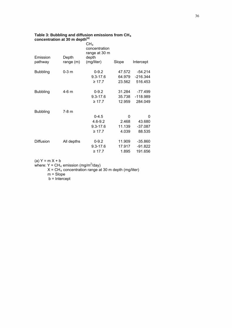
36

Table 3: Bubbling and diffusion emissions from CH4 concentration at 30 m depth(a)

Emission pathway

Depth range (m)

CH4 concentration range at 30 m depth (mg/liter) Slope Intercept

Bubbling 0-3 m 0-9.2 47.572 -54.214 9.3-17.6 64.979 -216.344 ≥ 17.7 23.562 516.453 Bubbling 4-6 m 0-9.2 31.284 -77.499 9.3-17.6 35.738 -118.989 ≥ 17.7 12.959 284.049 Bubbling 7-8 m 0-4.5 0 0 4.6-9.2 2.468 43.680 9.3-17.6 11.139 -37.087 ≥ 17.7 4.039 88.535 Diffusion All depths 0-9.2 11.909 -35.860 9.3-17.6 17.917 -91.822 ≥ 17.7 1.895 191.656 (a) Y = m X + b where: Y = CH4 emission (mg/m2/day) X = CH4 concentration range at 30 m depth (mg/liter) m = Slope b = Intercept

Parameter Value Units Source Above-ground fraction 0.759 Fearnside 1997b, p. 3Average depth of surface water zone 1 meter Assumption, based onLeaf decay rate in seasonally inundated zone -0.5 Fraction/year Assumption. Above-water decay rate (0-4 yrs) -0.1680 Fraction/year Assumed same as felleAbove-water decay rate (5-7 yrs) -0.1841 Fraction/year Assumed same as felleAbove-water decay rate (8-10 yrs) -0.0848 Fraction/year Assumed same as felleAbove-water decay rate (>10 yrs) -0.0987 Fraction/year Assumed same as felleCarbon content of wood 0.50 Fearnside and others

Average total biomass of forest at Babaquara 244 Mg/ha Revilla Cardenas (198 Above-ground fraction

Average water depth at minimum level 18.4 meters At 142 m above msl Average water depth at normal operating level 23.4 meters At 165 m above msl Initial biomass present: leaves 4.1 Mg/ha Calculated from total bInitial biomass present: wood above water 138.8 Mg/ha Calculated from total bInitial biomass present: below ground 58.8 Mg/ha Calculated from total b

Methane release by termites in forest 0.687 kg CH4/ha/year Martius and others 199Methane release by termites in above-water biomass per Mg C decayed through termites 0.0023 Mg CH4 Martius and others 199Percent of decay mediated by termites above the normal operating level waterline 4.23 % Martius and others 199Percent of decay mediated by termites below the normal operating level waterline 0 % Based on Walker and

Total area of reservoir at normal operating level 6,140 km2

Riverbed area 136 km2 Revilla-Cardenas 1988

Area cleared prior to flooding (permanently flooded zone) 0 km2

Total area of forest flooded 6,004 km2 Calculated by differenc

Original forest area of permanently flooded zone 2,424 km2 Area of zone, minus riv

Original forest area of drawdown zone 3,580 km2 Calculated by differenc

Rate of trunks breaking off at waterline for trees > 25 cm DBH 0.063

Fraction of original stock/year Based on Walker and

Rate of trunks breaking off at waterline for trees < 25 cm DBH 0.113

Fraction of original stock/year Based on Walker and othe

Rate of branch fall (and assumed fall of trunks above first branch) 0.094

Fraction of original stock/year Based on Walker and othe

Percent of above-ground live wood biomass in branches 30.2 % Fearnside 1995a, p. 12 baand trunk above first branch

Bole as percent of total live above-ground biomass in live trees > 10 cm DBH

57.47 % Based on biomass expansbiomass > 190 Mg/ha in liv

Above-ground live biomass < 10 cm DBH 22.2 Mg/ha Calculated from above Branches as percent of live bole biomass 51.4 % Based on Brown and LugoBranch biomass 55.9 Mg/ha Calculated from above Above-ground biomass of forest at Babaquara 185.3 Mg/ha Calculated from total and Above-ground live wood biomass 155.5 Mg/ha Total-leaves-dead Above-ground dead wood biomass 25.6 Mg/ha Klinge 1973, p. 179 Live bole biomass 108.6 Mg/ha Partioning based on BrowLive bole biomass 10-25 cm DBH 23.9 Mg/ha Partioning based on BrowLive bole biomass < 10 cm DBH 13.0 Mg/ha Jordan and Uhl 1978 Live bole biomass 0-25 cm DBH 36.9 Mg/ha Summed from above Live bole biomass > 25 cm DBH 71.7 Mg/ha Partioning based on BrowLive bole biomass: above waterline 96.4 Mg/ha Vertical distribution interpoLive bole biomass 0-25 cm DBH: above waterline 32.8 Mg/ha Vertical distribution interpoLive bole biomass > 25 cm DBH: above waterline 63.6 Mg/ha Vertical distribution interpoFraction of trees that float 0.4 Fraction Richard Bruce, personal cFraction of original branches on remaining trees falling per year 0.094 Fraction Calculated from Walker an

Average fraction of year drawdown area exposed 0.5 Fraction Rough estimate based on

BABAQUARA BELO MONTE Area

(km2) Percent

Above- ground Biomass loading(b) (Mg/ha dry weight)

Area (km2)

P Vegetation type

Unflooded vegetation Open terra firme forest

[mixed open forest (FA) + open submontane forest (FS)]

3,565.3 58.0 175.2 Open terra firme forest

on steeply sloping terrain 205.7

Open terra firme forest

on rolling terrain 11.9

Broadleafed secondary forest 10.9 0.2 20.0 (c)

11.0 Flooded vegetation Dense seasonally flooded riparian forest

or dense riparian forest (FC) 2,421.9 39.3 201.2 191.5

Open seasonally flooded riparian forest (Alluvial pioneer grassy formations)

5.6 0.1 60.0 No vegetation (river channel) Areas without plant cover 136.3 2.4 0.0 20.0 Totals Total unflooded vegetation 3576.3 58.2 228.5 Total flooded vegetation 2,427.5 39.4 191.5 Total vegetation 6,003.7 97.6 185.3 420.0 Total reservoir 6,140.0 100.0 440.0 (a) Data from Revilla Cardenas (1987, p. 55; 1988, p. 87), with areas adjusted in proportion to the current reservoir arefor Babaqura; 440 km2 for Belo Monte). (b) Values include dead biomass (litter and dead wood) vines and root mat

Item Value Units Source UPTAKE FROM UNFLOODED FOREST SOIL Average annual CH4 gas uptake -3.8 kg CH4/ha/year Potter and others (1996) from 22 studies from unflooded forest soil

Total area of forest flooded by reservoir 6,004 km2

Based on 6140 km2 reservoir area and streambed from Revilla Cardenas 1988, p. 87

Area of riparian forest flooded by reservoir 2,427 km2

Revilla Cardenas 1988, p. 87 Area of terra firme forest flooded by reservoir 3,576 km2 Calculated by difference Fraction of year riparian forest flooded naturally 0.17 Fraction Assumed 2 months on average Uptake per ha per year in riparian forest -3.17 kg CH4/ha/year Proportional to time unflooded Uptake per year in riparian forest -768.70 Mg CH4/year Uptake per ha × area of riparian forest Uptake per year in terra firme forest -1,358.98 Mg CH4/year Uptake per ha × area of terra firme forest Total uptake per year -2,127.68 Mg CH4/year Sum by forest type Global warming potential (GWP) of CH4 21 Mg CO2 gas equivalent/ Schimel and others 1996 Mg CH4 gas CO2 carbon equivalent/year -0.012 Million Mg CO2- Calculated from CH4 emission, GWP,

atomic weight of C (12) and molecular weight of CO2 (44)

equivalent C/year EMISSION BY FOREST TERMITES Emission/ha/year 0.5 kg CH4/ha/year Fearnside 1996b Ha-year equivalents of forest 0.6 Million ha-year equivalents Calculated from above Emission/year 317.0 Mg CH4/year Calculated from above CO2 carbon equivalent/year 0.0018 Million Mg CO2- Calculated as above equivalent C/year EMISSIONS FROM NATURAL FLOODING OF PRE-DAM FLOODED FOREST Methane emission of flooded forest during natural flooding

103.8 mg CH4/m2/day Mean of five studies in white-water várzea fore (Wassmann and Martius 1997, p. 140)

Days flooded per year 59.4 Days Assumption, as above Annual emission per km2

6.2 Mg CH4/year/km2 Calculated from above Annual natural emission by flooded forest 14,961 Mg CH4/year Calculated from above CO2 carbon equivalent/year 0.086 Million Mg CO2- Calculated from above equivalent C/year Annual annual emission adjusted for cycle length

44,883 Mg CH4/year Considering emission per cycle (2 months vs 6 months)

CO2 carbon equivalent/year

0.257 Million Mg CO2-equivalent Calculated from above C/year

EMISSIONS FROM PERIODIC PONDING EVENTS IN TERRA FIRME FOREST

2

Emission when flooded or ponded 103.8 mg CH4/m2/day Assumed same as várzea forest flooding

(as above). Annual natural emission by ponding 187.0 Mg CH4/year Calculated from above CO2 carbon equivalent/year 0.001 Million Mg CO2- Calculated from above equivalent C/year TOTALS

Total emission of methane 43,259 Mg CH4/year Calculated from above, including

cycle-length adjustment CO2 carbon equivalent/year 0.248 Million Mg CO2- Calculated from above equivalent C/year

Average annual N2O gas emission 8.7 kg N2O/ha/year Verchot and others 1999, p. 37

from unflooded forest soil

Total area of forest flooded by reservoir 6,004 km2

Based on 6140 km2 reservoir area and streambed from Revilla Cardenas, 1988, p.87

Area of riparian forest flooded by reservoir 2,427 km2

Revilla Cardenas 1988, p. 87 Area of terra firme forest flooded by reservoir 3,576 km2 Calculated by difference Fraction of year riparian forest flooded naturally 0.17 Fraction Assumed 2 months on average Emission per ha per year in riparian forest 7.23 kg N2O/ha/year Proportional to time unflooded Emission per year in riparian forest 1,755.6 Mg N2O/year Emission per ha × area of riparian forest Emission per year in terra firme forest 3,103.7 Mg N2O/year Emission per ha × area of terra firme forest

Total emission per year 4,859.3 Mg N2O/year Sum by forest type

Global warming potential (GWP) of N2O 310 Mg CO2 gas equivalent/ Mg N2O gas

Schimel and others 1996

CO2 carbon equivalent/year 0.411 Million Mg CO2-

equivalent C/year Calculated from area and per-hectare emission, atomic weight of C (12) and molecular weight of CO2 (44)

EMISSIONS FROM FLOODING Riparian forest flooding 404.6 km2-days/year Calculated from area and assumed

6-month average flood

Terra firme forest ponding 1,801.1 km2-days/year Calculated from area, 5% flooding per event

(based on Mori and Becker 1991) and assumed 5-year frequency a nd 30 day duration

Emission when flooded 7.6 kg N2O/km2-day 7.6 mg N2O/m2/day (Tucuruí and Samuel reservoir means from de Lima and others 2002)

Emission from riparian forest flooding 3.1 Mg N2O/year Flooding (km2/days) × emission/km2/day Emission from terra firme forest ponding 13.7 Mg N2O/year Ponding (km2-days) × emission/km2/day Total emission from flooding 16.8 Mg N2O/year sum of flooding emission CO2 carbon equivalent/year 0.001 Million Mg CO2- Calculated from GWP as above. equivalent C/year TOTAL EMISSION

Total emission from forest loss 4,876.0 Mg N2O/year Sum of unflooded forest, ponding and flooding emissions

CO2 carbon equivalent/year 0.412 Million Mg CO2- Calculated from GWP as above. equivalent C/year

Table 8: Greenhouse-gas emissions from dam and transmission-line construction Belo Monte Babaqu Item Units Emission

per unit CO2-equiv C (kg)

Ref- erence

Note No. of units

Ref- erence

Emission (million Mg CO2- equivalent C)

Note No. of units

Steel Mg 600.0 (a) (b) 323,333 (c) 0.194 (a) 30Cement kg 0.207 (a) (c) 848,666,000 (e) 0.176 (a) 1,217,25Diesel million kg 863,280 (d) 135.1 (f) 0.117 Electricity TWh 139,903,200 (g) 3.15 (h) 0.441 Dam sub-total 0.928 Transmission line construction

km-MW installed 1.9 (i) 29,596,901 (j) 0.055 (a) 17,04

Project total 0.983 (a) Van Vate 1995. (b) Uses IPCC 1994 100-year GWPs: CO2=1, CH4=24.5, N2O=320 (Albritton and others 1995). (c) Based on proportions relative to Belo Monte (see text). (d) Uses IPCC 1995 100-year GWP values [Kyoto Protocol values]: CO2=1, CH4=21, N2O=310 (Schimel and others 19(e) Based on concrete volumes (da Cruz 1996, p. 18)(see text). (f) Babaquara diesel use based proportional to planned excavation.

(g) Based on displacement of combined-cycle gas in São Paulo (see text). (h) Construction electricity use based on 280 kWh electricity/TJ (Dones and Gantner 1996). Emissions from electricitygeneration baseline in São Paulo (see text). (i) Mean in Québec, Canada (Peisajovich and others 1996).

(j) Transmission lines from Belo Monte to South-Central Brazil branch and go to three destinations with a mean distanc Cachoeira Paulista-SP (2662 km), Campinas-SP (2599 km) and Ouro Preto-MG (2680 km) (Brazil, MME-CCPESE 2 Babaquara has an additional 70 km of line.

Table 9: Long-term averages of net greenhouse-gas emission for the Belo Monte/Babaquara complex Emissions from all sources

(million Mg CO2-equivalent C/year) Years 1-10

10-year average

Years 1-20 20-year average

Years 1-50 50-year average

Inventory emissions Surface emissions 1.0 0.8 0.4 Turbines 2.6 3.8 2.8 Spillway 1.6 1.0 0.6 Transposition canal 0.2 0.4 0.3 Bottlenecks 0.01 0.01 0.01 Total inventory emissions 5.3 6.0 4.1 Other fluxes Fossil-fuel substitution -3.7 -3.9 -4.1 Pre-dam ecosystem fluxes -0.3 -0.5 -0.6 Above-water biomass 9.6 7.2 3.8 Shoreline decay 0.07 0.04 0.01 Total other fluxes 5.9 0.1 -5.5 Total impact 11.2 6.1 -1.4 Gross impact as multiple of fossil-fuel baseline 4.0 2.5 0.7

1

Table 10: Sensitivity tests for selected input parameters

Input parameter

Units

Reference scenario parameter value

Percent change in total impact in response to a 10% increase in input parameter

10-year average

20-year average

50-year average

Proportion of CH4 released at turbines (midpoint of high and low scenarios)

Proportion 0.55

Percent change % 2.03 5.18 -16.17 Proportion of CH4 released at spillway Proportion 1 Percent change 1.22 1,37 -3.67 Growth rate of drawdown zone vegetation Mg/ha/year

dry weight 10

Percent change % 0.02 0.46 -3.33 Biomass of macrophytes, years 1-6 Mg/ha of

macrophytes dry weight

11.1

Percent change % 0.23 0.26 -0.54

Biomass of macrophytes, years 7-50 Mg/ha of macrophytes 1.5

Percent change % 0.003 0.10 -0.48 Unbeached macrophytes (death+decay)

fraction per month 0.144

Percent change % 0.23 0.34 -0.92 Flooded drawdown (underwater decay rate)

fraction per month 0.656

Percent change % 0.02 0.48 -0.04

Beached macrophyte decay rate fraction per month 0.314

Percent change % -0.001 -0.01 0.04

Above-ground biomass Mg/ha dry weight 176.1

Percent change % 2.95 5.02 -11.91 Adduction canal emission percent % 15.3 Percent change % 0.02 0.08 -0.26 Adduction canal oxidation percent % 66.5 Percent change % -0.50 -2.49 7.90 Bottlenecks emission percent % 2.1 Percent change % 0.01 0.004 0.002 Bottlenecks oxidation percent % 9.2

2

Percent change % -0.01 -0.07 -0.04 Shoreline mortality percent: 0-100 m (weighted average)

% 81.7

Percent change % 0.06 0.07 -0.04

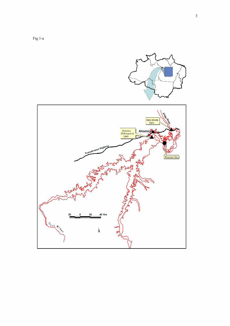
3

Fig 1-a

4

Fig 1-b

5

Fig. 2

CH4 concentration at 30 m depth vs Mg C/billion m3 water

CH

4 co

ncen

trat

ion

at

30 m

(mg/

l)

25

20

15

10

5

05,000 10,000 0 15,000 20,000 25,000

Anaerobic decay (Mg C/billion m3 of water)

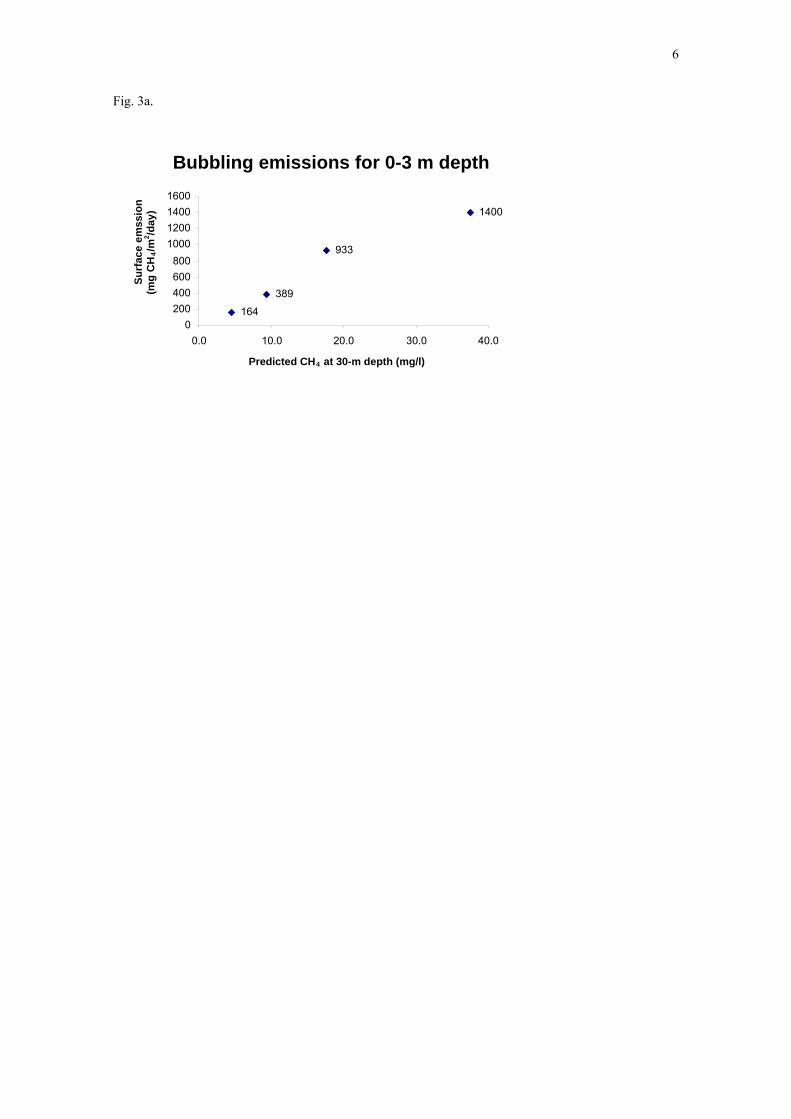
6

Fig. 3a.

Bubbling emissions for 0-3 m depth

4006008

(mg

CH 00

1000120014001600

Surf

ace

emss

ion

4/m

2 /day

) 2

164

389

933

1400

2000

0.0 10.0 20.0 30.0 40.0

Predicted CH4 at 30-m depth (mg/l)

7

Fig 3b.

Bubbling emissions for 4-6 m depth

0100200300400500600700800900

Surf

ace

emis

sion

s (g

CH

4/m2 /d

ay)

66

214

513

770

10.0 40.0 0.0 20.0 30.0

Predicted CH4 at 30 m depth (mg CH4/l)

8

Fig. 3c.

Bubbling emissions for 7-8 m

300

55 67

160

240

Surf

ace

emis

sion

(gC

H4/

m2 /d

ay) 250

200

150

100

50

0 0.0 10.0 20.0 30.0 40.0

Predicted CH4 at 30 m depth (mg CH4/l)

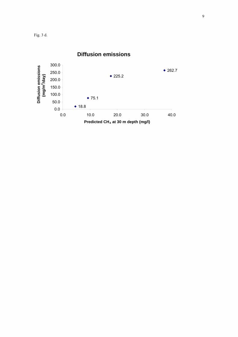
9

Fig. 3 d.

Diffusion emissions

300.0

18.8

75.1

225.2262.7

Diff

usio

n em

issi

ons

(mg/

m2 /d

ay) 250.0

200.0

150.0

100.0

50.0

0.00.0 10.0 40.0 20.0 30.0

Predicted CH4 at 30 m depth (mg/l)

10

Fig. 4a

Babaquara: Carbon decayed anaerobically

8

Car

bon

deca

yed

per y

ear (

mill

ion

Mg)

7

6

TotalDrawdown regrowthSoil CMacrophytesOriginal leaves

5

4

3

2

1

016 19 1 4 7 22 25 28 31 34 37 40 43 46 4910 13

Year

11

Fig. 4b

Belo Monte-Channel Reservoir: Carbon decayed anaerobically

0.40

Car

bon

deca

yed

per y

ear (

mill

ion

Mg)

0.35

0.30

Original leaves0.25

Macrophytes

0.20 Soil C

Drawdown regrowth0.15 Total

0.10

0.05

0.00 13 1 4 7 16 19 22 25 28 31 34 37 40 43 46 4910

Year

12

Fig. 4c

Belo Monte Canals Reservoir: Carbon decayed anaerobically

0.12

Car

bon

deca

yed

per y

ear (

mill

ion

Mg)

0.10 Original leaves

Macrophytes0.08

Soil C

Drawdown regrowth0.06 Total

0.04

0.02

0.00 13 1 4 7 16 19 22 25 28 31 34 37 40 43 46 4910

Year

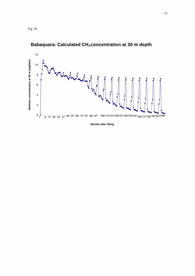
13

Fig. 5a

Babaquara: Calculated CH4 concentration at 30 m depth

12

Met

hane

con

cent

ratio

n at

30

m (m

g/lit

er)

10

8

6

4

2

0 49 209 201

1 9 17 25 33 41 57 65 73 81 89 97 105113121129137 145153161 177 185 193169

Months after filling

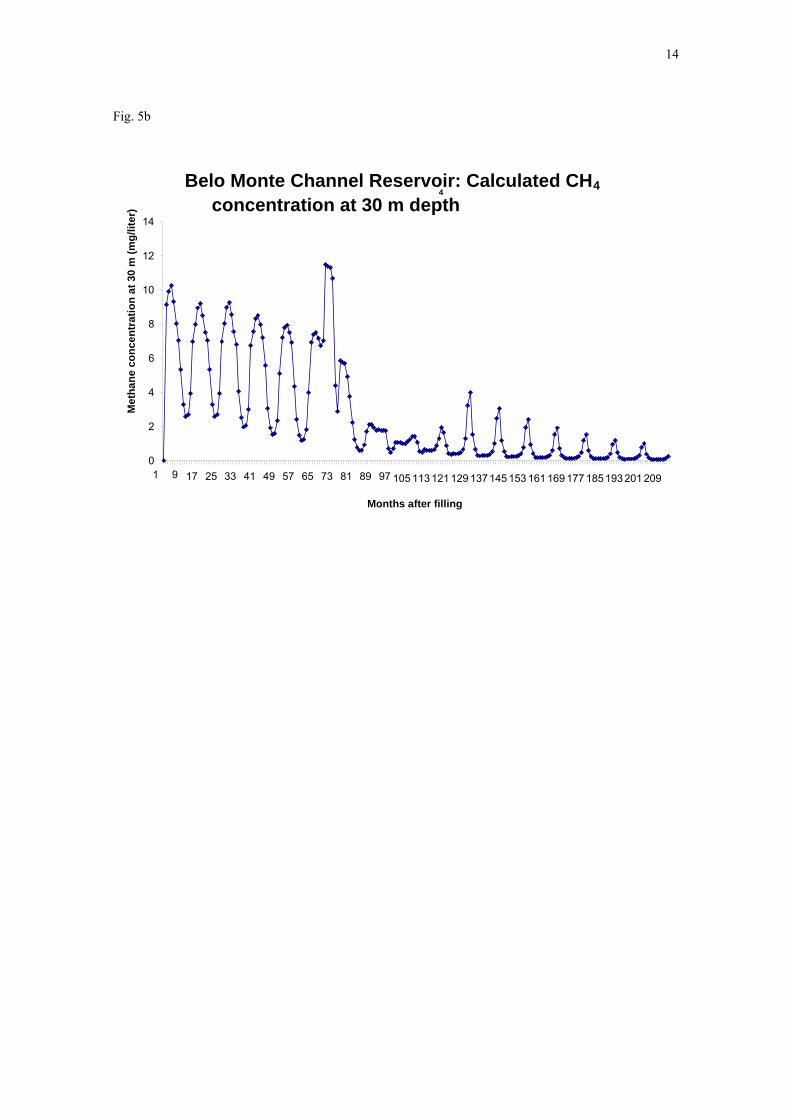
14

Fig. 5b

Belo Monte Channel Reservoir: Calculated CH4 4

concentration at 30 m depth

Met

hane

con

cent

ratio

n at

30

m (m

g/lit

er)

14

12

10

8

6

4

2

057 1 9 169 185 201 65 73 81 89 9717 25 33 41 49 177 193 209105 113 121 129 137145 153 161

Months after filling

15

Fig. 5c

Belo Monte Canals: Calculated CH4 4

concentration at 30 m depth 25

Met

hane

con

cent

ratio

n at

30

m (m

g/lit

er)

20

15

10

5

01 9 17 41 177 185 19325 33 49 57 65 73 81 89 97 201 209105 113 121 129 137 145153161169

Months after filling

16

Fig. 6

Belo Monte + Babaquara Reservoir emissions 25 Bottlenecks

-15

-10

-5

0

5

10

15

20

1 3 5 7 9 11 13 15 17 19 21 23 25 27 29 31 33 35 37 39 41 43 45 47 49

Year

Turbines

Spillway A

nnua

l em

issi

on (m

illio

n M

g C

0

Fossil FuelsubstitutionPre-dam ecosystems2-

equi

vale

nt

C)

Above-water biomass

Total impact

Shoreline decay

Adduction canal

Surface

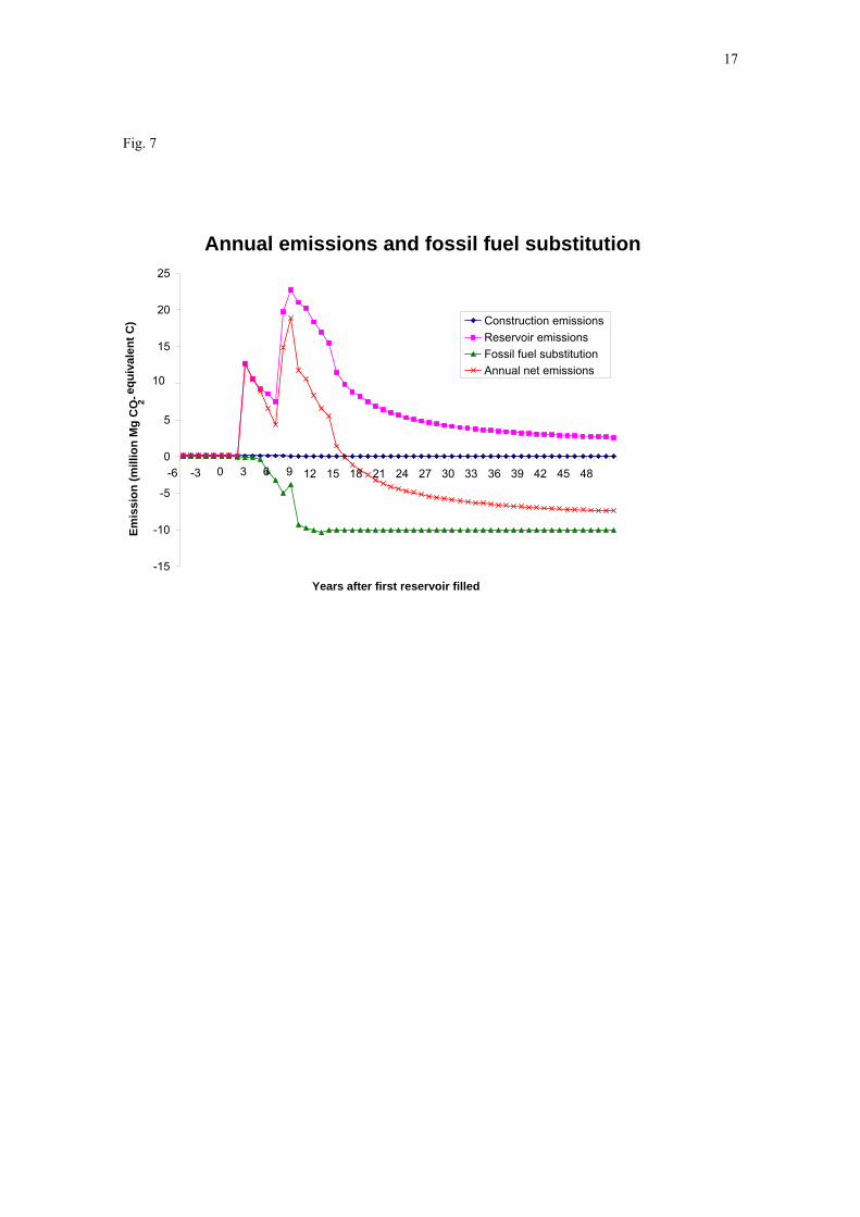
17

Fig. 7

Annual emissions and fossil fuel substitution 25

20Construction emissions

equi

vale

nt C

)

Reservoir emissions15 Fossil fuel substitution

Annual net emissions10

Emis

sion

(mill

ion

Mg

CO

- 2

5

0 9 15 0 3 6-6 -3 12 18 21 24 27 30 33 36 39 42 45 48

-5

-10

-15

Years after first reservoir filled

18

Fig. 8

Cumulative net impact of Belo Monte + Babaquara

150

Cum

ulat

ive

net g

loba

l-war

min

g im

pact

100

(mill

ion

Mg

C)

50

0

-100

-50

1 3 5 7 9 11 39 43 13 15 17 19 21 23 25 27 29 31 33 35 37 41 45 47 49

Year

19

Fig. 9

Discounted annual net emissions

25

20

2

-10

-5

0

5

10

15

-6 -4 -2 0 2 4 6 8 10 12 14 16 18 20 22 24 26 28 30 32 34 36 38 40 42 44 46 48 50

Years after filling first reservoir

Dis

coun

ted

annu

al n

et e

mis

sion

s -e

quiv

alen

t C

0% discount1% discount2% discount3% discount

(mill

ion

Mg

CO

2

20

Fig. 10

Discounted cumulative emissions150.0

0% discount

1% discount

-100.0

-50.0

0.0

50.0

100.0

-6 -4 -2 0 2 4 6 8 10 12 14 16 18 20 22 24 26 28 30 32 34 36 38 40 42 44 46 48 50

Years since filling first reservoir

2% discount

Cum

ulat

ive

net e

mis

sion

s

-equ

ival

ent C

)

3% discount

2(m

illio

n M

g C

O

21

Fig. 11 Discounted net impact

-2.0

-1.5

-1.0

-0.5

0.0

0.5

1.0

0 1 2 3 4 5 6 7 8 9 10 11 12

Annual discount rate (%)

Net

ann

ual i

mpa

ct

(mill

ion

Mg

CO

2-eq

uiva

lent

C)