feasibility of a wind-propelled spar buoy for use as a
TRANSCRIPT

Feasibility of a Wind-Propelled Spar Buoy for Use as
a Meteorological Observation Platform in Hurricane Conditions
Andreas S. von Flotow
A thesis
submitted in partial fulfillment of
the requirements for the degree of
Masters of Science in Aeronautics and Astronautics
University of Washington
2014
Committee:
Dr. Kristi Morgansen
Dr. Juris Vagners
Program Authorized to Offer Degree:
William E. Boeing Department of Aeronautics and Astronautics

2
©Copyright 2014
Andreas S. von Flotow
3
Feasibility of a Wind-Propelled Spar Buoy for Use as
a Meteorological Observation Platform in Hurricane Conditions
University of Washington
Abstract
Andreas S. von Flotow
A novel vehicle concept is introduced and its feasibility as an autonomous, self-propelled
weather buoy for use in violent storm systems is analyzed. The vehicle concept is a spar sailboat
– consisting of only a deep keel and a sailing rig; no hull – a design which is intended to improve
longevity in rough seas as well as provide ideal placement opportunities for meteorological
sensors. To evaluate the hypothetical locomotive and meteorological observation capabilities of
the concept sailing spar in hurricane-like conditions, several relevant oceanographic phenomena
are analyzed with the performance of the concept vehicle in mind. Enthalpy transfer from the
ocean to the air is noted as the primary driving force of tropical storms and therefore becomes
the measuring objective of the sailing spar. A discrete, iterative process for optimizing driving
force while achieving equilibrium between the four airfoil surfaces is used to steer the sailing
spar towards any objective despite variable and opposing simulated winds. Based on the
limitations of sailing theory, logic is developed to autonomously navigate the sailing spar
between human-selected waypoints on a digitized geographic map. Due the perceived inability to
measure air-sea enthalpy exchange because the nature of tropical storms and due to its small
scale, the sailing spar is deemed infeasible as a hurricane-capable meteorological observation
platform.
Chair of the Supervisory Committee:
Associate Professor Kristi Morgansen
William E. Boeing Department of Aeronautics and Astronautics

4
I. CONTENTS
I. Contents .................................................................................................................................... 4
II. Nomenclature ....................................................................................................................... 5
1) Superscripts ...................................................................................................................... 5
2) Subscripts ......................................................................................................................... 7
III. Introduction and Design Criteria ......................................................................................... 8
A. Tropical Cyclone Measurements and Modeling ................................................................ 10
B. Unmanned Sailing Navigation and Simulation.................................................................. 13
C. Spar Design Features ......................................................................................................... 23
IV. Design Approach and Methodology .................................................................................. 27
A. Measuring and Simulating Oceanographic Phenomenon .................................................. 27
B. Aero- Hydrodynamics Simulations .................................................................................... 38
C. Navigation Simulations ...................................................................................................... 47
D. Modeling Assumptions ...................................................................................................... 57
V. Results and Analysis .......................................................................................................... 59
A. Measurements of Simulated Oceanographic Phenomenon ................................................ 59
B. Simulation of Unmanned Sailing ....................................................................................... 81
C. Simulated Autonomous Navigation ................................................................................. 112
VI. Findings and Evaluation of Design .................................................................................. 114
A. Oceanographic Simulations ............................................................................................. 114
B. Vehicle Design Considerations ........................................................................................ 115
C. The Autonomous Navigator ............................................................................................. 117
VII. Conclusion ....................................................................................................................... 119
VIII. References ........................................................................................................................ 124
5
II. NOMENCLATURE
1) Superscripts
A cross sectional area
AR aspect ratio
c chord length
CD drag coefficient
CL lift coefficient
CK enthalpy exchange coefficient
D diameter
Dν mass diffusion coefficient
e Oswald Efficiency Factor
FAR net force parallel to course
FAS net force perpendicular to course
FD drag force
FL lifting force
Fnet net aerodynamic force
HK enthalpy transfer across the air-sea interface or Hamiltonian
k wave number
ka specific enthalpy of the air
ks specific enthalpy of the water surface
L lever arm
Lv latent heat of vaporization of water
M wave direction divisions
Mw pitching moment of the sail

6
Mt pitching moment of the trim tab
m mass
N wave frequency divisions
q humidity of the air
R roll rate scaling factor
r wave amplitude
RM mast-top rolling motion
T air temperature
t time variable
Ts sea surface temperature
Um wind speed
VA apparent wind speed
Vg gust propagation speed
Vs speed of ASV
Vs.s. steady state speed
Vt true wind speed
wa surface humidity
ws free stream humidity
X horizontal direction on ocean surface
x heading of ASV
Y vertical direction out of ocean surface
y perpendicular of ASV heading
Z horizontal direction on ocean surface, perpendicular to X direction

7
α angle-of-attack of the sail with the apparent wind
β apparent wind angle
δ trim tab pitch or net force angle from course perpendicular
θ angle of net force relative to lifting force vector
λ heading angle relative to course; leeway angle
μ mean
ρ density
σ standard deviation
ψ true wind angle
ω angular frequency
ϕ wave direction
2) Subscripts
a air
d downwash
f friction
g gust
i induced
k keel of vehicle
s wing-sail or surface or vehicle
t trim tab or true value relative to fixed frame
w wing-sail
8
III. INTRODUCTION AND DESIGN CRITERIA
There is a deficit in the temporal and spatial resolution of oceanographic measurements
provided by contemporary observation platforms.[1]
As explicitly stated by the Ocean
Observatories Initiative, in order to realize more accurate weather forecasting models,
meteorologists need higher density and quality of measurements to be supplied by in situ
observation platforms[2]
– a task especially well-suited to autonomous surface vehicles (ASV’s).[3]
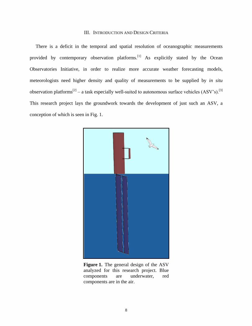
This research project lays the groundwork towards the development of just such an ASV, a
conception of which is seen in Fig. 1.
Figure 1. The general design of the ASV
analyzed for this research project. Blue
components are underwater, red
components are in the air.

9
Available autonomous observation platforms are incapable of maintaining a presence during
hurricanes, just when observations are most relevant.[3]
Unmanned weather reconnaissance
aircraft, touted as offering long range at a “semi-disposable” price, cost thousands of dollars per
flight-hour and frequently do not return.[4], [5]
Established seafaring robots such as drifting buoys,
Seagliders[6]
, and Wave Gliders[7]
, although low cost and capable of long endurance, are only
marginally mobile and far too slow for wide range deployments.
This document presents the initial findings from an investigation into the feasibility of an
energy-independent ASV, seaworthy enough to loiter for months in areas of severe
meteorological development (i.e. hurricanes) yet fast enough to make observations in remote
corners of the globe on weeks’ notice, while reliable and low cost. Alternative uses for the vehicle
– outside of hurricane surveillance – are proposed. There appears to be a demand for persistent,
mild-weather surveillance platforms as well as self-propelled sonar buoys, both of which missions
are well within the capabilities of the ASV. Several iterations of a wind-propelled, solar-powered
ASV are considered with the primary academic goal of developing a novel control process for
such a vehicle. A secondary, hypothetical objective – as of yet to be achieved – is to deploy a
prototype vehicle tasked as a self-propelled weather station buoy, for concept proofing.
In order to quantify the robustness of the autonomous controller developed herein when
satisfying the primary academic goal of this investigation, key behaviors of the ASV control
system were simulated computationally. The virtual controller responses include hydrodynamic
response, control feedback, sensor noise filtering, and navigation. Results of these simulations are
discussed in the following pages. The performance of each simulated control feature of the ASV
is evaluated against criteria necessary for ocean deployment. Several phenomenon of physical
oceanography were also simulated in the fluid dynamics laboratory to gain a better understanding
10
of the potential efficacy the ASV might have as a roving sensor platform. The oceanographic
phenomenon experiments included measuring the temperature and velocity boundary layer
gradient profiles of a column of water, recording the acoustic and thermodynamic dissipation of
splash droplets, and quantifying the cooling and evaporation of a ballistic water droplet.
A. Tropical Cyclone Measurements and Modeling
As part of this research project to develop an autonomous sailing vehicle, the ability of said
vehicle to collect meteorological observations under hurricane conditions was evaluated. In
general, making high-resolution meteorological measurements is difficult. Making these
measurements is especially difficult during intense storm conditions.[8], [9]
Very few existing
meteorological observation platforms and no known ASVs are capable of persisting through
tropical cyclones.[9], [10]
The sea state is far too rough and the winds are too high. Taking sea
surface measurements under these circumstances is nearly impossible using contemporary
methods. Data collection of hurricane conditions is currently limited to low-resolution satellite
images and single-use dropsondes, both of which are exorbitantly expensive yet still provide
unsatisfactory measurements.[11]
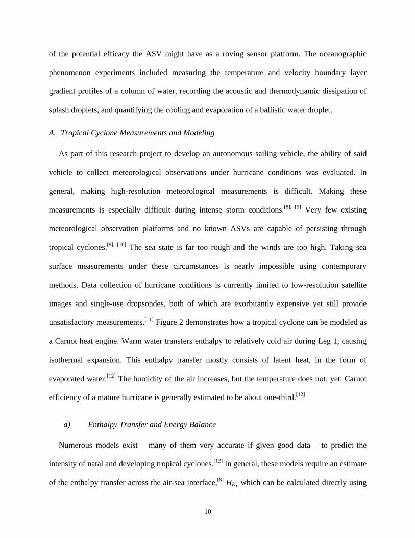
Figure 2 demonstrates how a tropical cyclone can be modeled as
a Carnot heat engine. Warm water transfers enthalpy to relatively cold air during Leg 1, causing
isothermal expansion. This enthalpy transfer mostly consists of latent heat, in the form of
evaporated water.[12]
The humidity of the air increases, but the temperature does not, yet. Carnot
efficiency of a mature hurricane is generally estimated to be about one-third.[12]
a) Enthalpy Transfer and Energy Balance
Numerous models exist – many of them very accurate if given good data – to predict the
intensity of natal and developing tropical cyclones.[12]
In general, these models require an estimate
of the enthalpy transfer across the air-sea interface,[8]
HK¸ which can be calculated directly using

11
measurements of the sea surface temperature, Ts, the air temperature, T, the humidity, q, and the
wind speed, Um.[10]
The equations (1.1)-(1.3) relate these variables, using the measures of specific
enthalpy of the water surface, ks, and the air, ka;[12]
𝐻𝐾 = 𝜌𝐶𝐾𝑈𝑚(𝑘𝑠 − 𝑘𝑎). (1.1)
𝑘𝑎 = (1 − 𝑞)𝑐𝑝𝑇 + 𝑞(𝐿𝑣 + 𝑐𝑝𝑣𝑇). (1.2)
𝑘𝑠 = 𝑓𝑢𝑛𝑐. {𝑇𝑠}. (1.3)
The relationship represented by (1.1) represents total energy transfer including latent heat in
the form of evaporation. The factor CK takes into account spray and waves, which can increase
latent heat transfer by increasing the available surface for evaporation. Lv is the latent heat of
vaporization of water.
Figure 2. The Carnot cycle as applied to a hurricane.[11]
Distance from eye of storm Hei
ght
of
storm

12
In (1.1) the most difficult parameter to estimate is the enthalpy exchange coefficient CK
because sea spray, spume, and breaking waves are difficult to quantify and measure.[8]
Figure 3
depicts a wave crest in mild hurricane conditions. Spume drops are picked up off the wave crest
and carried through the air. Drops of water evaporate more quickly than water from the ocean
since they present a greater surface area per volume ratio to the passing wind.
When the fast-evaporating drops of spume land back into the ocean, they create a splash. The
splashed-up droplets are also caught by the wind and may, too, evaporate and transfer latent heat
to the air.
Figure 3. Spume droplets increase enthalpy transfer by evaporating as
they fly through the air, and by creating splash droplets, which also
evaporate.[12]
Since the initial spume drops had been evaporating along their trajectory previous to re-entry,
they are somewhat cooler than the secondary impact splash droplets. Therefore, the splashed-up
droplets, being warmer, will evaporate more quickly. In powerful cyclones, it is estimated that up
to fifty-percent of all enthalpy transfer occurs by spume droplet evaporation.[8], [10]

13
b) Autonomous Observation of Enthalpy Exchange
The efficacy of the ASV as a meteorological observation platform was analyzed with regards
to air-sea interactions. Specifically, the feasibility of a sailing spar device for collecting data
related to the enthalpy transfer – the missing data – inside a tropical cyclone was under
investigation. Three different methods by which enthalpy transfer data might be gathered were
examined in the following sections. The first method involved directly measuring the
temperatures, wind speed, and humidity over time.
The second method used underwater microphones to detect the acoustic signatures of
impacting spume droplets, from which the size of each droplet and its evaporation history might
be approximated. The third method to estimate air-sea enthalpy transfer used wind speed to
estimate the size and velocity of spume droplets, from which their impact dynamics may be
predicted as well as the total evaporation caused by primary and secondary spume and splash
droplets. The third method asked the question: are the splashed-up droplets made of cold, re-
entering spume water or warm ocean water thrown up by the impacting spume droplet?
B. Unmanned Sailing Navigation and Simulation
Contemporary robotic sailing platforms have been engineered for calm weather; they do not
stand up to environmental stresses such as rough seas, strong winds, and the wear of sustained
deployment. The Microtransat regatta, which every summer poses the challenge of sailing an
autonomous boat across the Atlantic, has been running since 2009, and has yet to name a
winner,[3]
the farthest competitor making it just over 200 kilometers before wrecking. Harbor
Wing Tech, a Seattle-based robotic sailboat company, has built a high functioning, autonomous
prototype. However, their prototype is not suitable for the open ocean due to its inability to self-
right after capsizing.[3]

14
a) Static Equilibrium Performance Evaluation
Autonomous sailing control is generally treated as a tracking problem whereby a desired
trajectory is followed in a constant, uniform wind vector field.[13], [14]
The goal of the controller is
to steer the wind propelled vehicle along the given trajectory while maximizing the aerodynamic
forces in the direction of desired motion. Treating both the sail and the keel of the ASV as airfoils,
aerodynamic forces are governed by the angle-of-attack between the wing-sail and the wind, and
the angle-of-attack between the hydrofoil keel and the passing water.[11]
This model of a sailboat
is constrained by force equilibrium between the wing-sail airfoil and the keel hydrofoil.[11]
In order to evaluate the theoretical performance of the sailing vehicle which was designed for
this project, a model was created and a series of simulations were run using Matlab software. The
model behavior is based on Bernoulli’s macro-aerodynamic principles and essentially treats the
sailing vehicle as a group of airfoil surfaces. Given the desired trajectory of sail and the wind
velocity, the simulations predict the static equilibrium heel, pitch, and leeway angles as well as
the equilibrium sailing speed of the spar vehicle. Many refining details applicable to airfoil
modeling were omitted from the simulation for simplicity. The research ASV was further
modeled with SolidWorks drawing software and more simulations were run using computational
fluid dynamics (CFD).
b) Sensor Noise Simulation and Filtering
Noisy data was simulated for several sensors and four different filtering methods are used to
parse the signal. The measurements and noise were artificially generated but were meant to
represent the output of wind velocity sensors on an ASV. There were two pairings of two sensors
each: an anemometer and wind vane atop the sail, and a force and position sensor associated with
the airfoil position actuation servo-motor.

15
Figure 4. The net lift-drag aerodynamic force, Fnet, t, and
pitching moment, Mt, generated by the trim tab (small airfoil
behind the wing-sail) act on the lever arm of length L to counter-
act the pitching moment, Mw, of the sail and maintain the desired
angle-of-attack, α, with the apparent wind, VA. The trim tab pitch,
δ, is maintained by a servo-motor.
Noise in the sail-top weather sensors is due partially to Gaussian measurement noise occurring
within the sensors, but for the most part comes from the rolling motion of the vehicle at sea, as
well as vortices presumed to form at the tip of the sail. This weather noise is biased and after
attempting to filter it with an Extended Kalman Filter, the bias is partially removed by heuristic
methods. Noise in the servo-motor sensors is Gaussian and zero-mean and is filtered via a
discrete, linear Kalman Filter. A moving average filter improves on the Kalman Filter.
The trim tab seen sticking off towards the right in Fig. 1 is used to point the wing-sail into the
wind at a desired angle-of-attack such that the resulting lift force will propel the ASV forward.
Figure 4 shows a simple schematic of how the trim tab functions. In order to maintain a desired
sail angle-of-attack, α, it is necessary to know the current apparent wind velocity, VA. For a given

16
wind speed and wind direction, relative to the desired course of travel, a trim tab pitch, δ, can be
analytically determined which will achieve a corresponding α. But first the wind velocity must be
found.
The ASV is equipped with two sensors to ascertain the direction and speed of the apparent
wind and two sensors for determining what angle-of-attack the wing-sail is holding. The two wind
sensors are an anemometer and direction indicator atop the wing-sail, and the two angle-of-attack
sensors are a servo-motor force and servo-motor position sensor in the trim tab actuator. A
plausible example of the anemometer and wind vane is seen in Fig. 5.
c) Line Following and Hydrodynamic Stall Avoidance
Even the most efficient sailboat in the world cannot sail directly upwind.[14]
As demonstrated
in Fig. 6, when starting from rest a sailboat must first turn downwind to pick up speed before
taking the desired heading. If a turn upwind is made too soon, the hull will stall in the water and
the boat will drift. In order to evaluate and iteratively improve the performance of the ASV, a
computer model was created to predict the acceleration and steady state velocity from a given
wind speed and wind direction along a desired heading.
The route taken by the ASV as it accelerates downwind from standstill is reminiscent of a
second-order damped impulse-step response, seen in Fig. 7. As every experienced sailor knows,
when performing the acceleration maneuver shown in Fig. 6, there is an optimal route which
minimizes the time spent hauling downwind, yet still quickly achieves the steady state velocity.
17
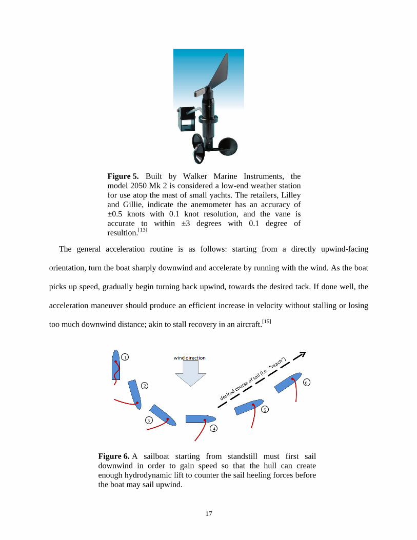
Figure 5. Built by Walker Marine Instruments, the
model 2050 Mk 2 is considered a low-end weather station
for use atop the mast of small yachts. The retailers, Lilley
and Gillie, indicate the anemometer has an accuracy of
±0.5 knots with 0.1 knot resolution, and the vane is
accurate to within ±3 degrees with 0.1 degree of
resultion.[13]
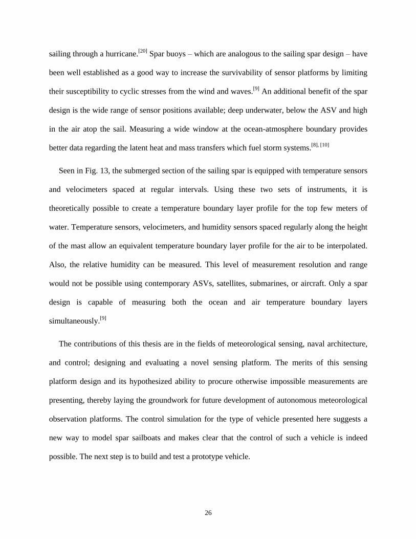
The general acceleration routine is as follows: starting from a directly upwind-facing
orientation, turn the boat sharply downwind and accelerate by running with the wind. As the boat
picks up speed, gradually begin turning back upwind, towards the desired tack. If done well, the
acceleration maneuver should produce an efficient increase in velocity without stalling or losing
too much downwind distance; akin to stall recovery in an aircraft.[15]
Figure 6. A sailboat starting from standstill must first sail
downwind in order to gain speed so that the hull can create
enough hydrodynamic lift to counter the sail heeling forces before
the boat may sail upwind.
1
2
3
4
5
6

18
This acceleration maneuver is optimized by reaching the steady state velocity as quickly as
possible. (1) explicitly enunciates the desired performance of the control algorithm: to reach
ninety five percent of steady state velocity, Vs.s., within the time it would take to sail 50 meters at
said steady state velocity. The Matlab System Identification Toolbox was used to generate a series
of single-input, single-output (SISO) estimation models from the wind angle inputs and boat
velocity outputs. A heuristic Monte Carlo simulation was run using different “damping” and
“natural frequency” values in the second-order impulse representation of the acceleration
maneuver. Steady state velocity was achieved soonest – as defined by (2) – using the parameters
that generated Fig. 7;
𝑡95% ≤ 50𝑚/𝑉𝑠.𝑠.. (2)
To attain the goal presented in (1), the system which describes the relationship between the
wind direction and the boat speed must be identified. The boat trajectory must be vectored such
that the wind direction inputs achieve the desired boat velocity outputs; shorter settling time.
Figure 7. The optimal path when accelerating from
standstill is expected to resemble a second or third order
under-damped step response. The step magnitude is the
desired tack. Overshoot is intended to maximize
acceleration.
0 5 10 15 20 250
20
40
60
Input-Output
time [seconds]
Tru
e W
ind
An
gle
[ d
eg
]
True Wind Speed and Acceleration Time V
t = 5.14 [m/s]
t( 95% ) = 13.6 [seconds]
True Wind Angle (input)
Boat Speed (output)
0 5 10 15 20 250
0.2
0.4
0.6
0.8
1
1.2
1.4
Boa
t S
pe
ed [
m/s
]

19
The wind direction inputs are expected to take the form of an underdamped second-order step
response, or perhaps the sum of an impulse and step response. However, regardless of the
efficiency of the acceleration maneuver, certain courses relative to the wind simply cannot be
taken by the ASV.
Figure 8 shows, in darker grey, the “no-go zone” reaches where sailing is unstable. Reaches
taken too far upwind will cause the hull of the ASV to stall in the water and the vehicle will drift
downwind. Sailing directly downwind requires the sail to be used as a blunt parachute. Courses
that require sailing into the no-go zones must be achieved by tacking or jibing – turning between
port and starboard reaches and zigzagging through the no-go heading.
Figure 8. A sailboat cannot travel directly
upwind and, with a wing-sail, it is difficult to
travel downwind. So, the ASV is limited to
crosswind reaches and must tack or jibe through
the grey no-go zones.[12]

20
Sailing a zigzag course upwind or downwind would, of course, not allow for perfect following
of the desired path. To maintain some semblance of line following during no-go zone traverses, a
cost function can be applied. Straying too far from the desired course incurs increasing costs; this
is known as a “tunnel cost” – as illustrated in Fig. 9.[12]
Turning too often in order to tightly follow the desired course is also an inefficient behavior
since each turning operation loses momentum. Therefore a turning cost is also implemented.
These cost functions are seen in (3). Figure 9 shows a hypothetical journey of the ASV,
attempting to follow a desired course but making several tacking turns upwind;
turning cost = 𝑓𝑢𝑛𝑐. |𝜆𝑐𝑢𝑟𝑟𝑒𝑛𝑡 − 𝜆𝑛𝑒𝑤| (3.1)
tunnel cost = 𝑓𝑢𝑛𝑐. |𝑥, 𝑦𝑐𝑢𝑟𝑟𝑒𝑛𝑡 − 𝑥, 𝑦𝑛𝑒𝑤|. (3.1)
This tunnel cost is not linear; missing the ends of the line incurs a much higher cost than
straying from the middle. Likewise, the turning cost is not linear; there is an absolute boundary
beyond which no sailing is permitted – this insures against collisions with land.
Figure 9. A sailboat cannot travel directly upwind and,
with a wing-sail, it is difficult to travel downwind. So, the
ASV is limited to crosswind reaches and must tack or jibe
through the grey no-go zones.

21
d) Wing-sail Aero- Hydrodynamics
An in-depth analysis of a wind- and solar-powered ASV was written by Patrick Rynne at the
Florida Atlantic University.[10]
In his analysis, Rynne develops a preliminary model for an
autonomous sailboat of contemporary hull design. He describes the optimal angle-of-attack for
the sail, given the true wind vector and velocity vector of the boat.
Rynne uses a wing-sail – similar to the design examined in this paper. He runs a numerical
optimization to determine the best airfoil shape of the wing-sail. The airfoil design he finally
decides on is close to a NACA0012, which is the cross-section used in the wing-sail and trim tab
of the ASV presented in this research.
The free-body diagram of the wing-sail used by Rynne is shown in Fig. 10. It treats the ASV
direction of travel as the reference, with the wind moving relative this course vector.
Figure 10. Rynne’s model of his ASV wing-sail, showing the
aerodynamic forces generated relative to the angle-of-attack in (a),
where the apparent wind, VA, is seen in (b) to be the difference
between the true wind, Vt, and the ship velocity, Vs. The forces can
be broken down into components acting parallel and perpendicular
to the ship velocity, as shown by (c).[11]

22
In his paper, Rynne notes that the wing-sail will operate under optimal conditions – that is, the
lift-to-drag ratio will be maximized – at a certain angle of attack, α, with respect to the apparent
wind.
As demonstrated in Fig. 11, when hauling downwind the apparent wind angle-of-attack, α,
may generate a lower lifting force in the direction of travel, FAR, than simply turning the sail
sideways and presenting a blunt surface area to the passing wind. Although Rynne simulates this
mode of sailing in his calculations, it is not adopted for the sailing spar for two reasons: it is not
necessary but rather counterproductive, and it creates dangerous stresses in the wing-sail pointing
mechanism.
Sailing a boat directly downwind imposes controllability challenges as the speed of the vehicle
catches up to the wind speed and – when surfing down the leeward side of a wave – surpasses the
wind speed.
Figure 11. The lift-generating approach of (a) can be
effectively replaced by the blunt object, drag-generating
method of (b) when sailing down-wind at an apparent wind
angle, β, of 135° to the wind.[11]

23
Rynne presents the aerodynamic equations used for estimating lift and drag forces, FL and FD,
respectively, generated by an airfoil in (4). The area of the airfoil, A, and density of air, ρ, must be
found beforehand.[11]
(4) is also applicable to liquids such as water;
𝐹𝐿 = ½ 𝐶𝐿 𝜌 𝑉𝐴2 𝐴 (4.1)
𝐹𝐷 = ½ 𝐶𝐷 𝜌 𝑉𝐴2 𝐴. (4.2)
The coefficients of lift and drag, CL and CD, respectively, for the airfoils used by Rynne, are
functions of α, as in (5).[11]
Ideally, the ratio between CL and CD should be minimized thereby
generating the highest lift for the smallest drag;
𝐶𝐿 = − 0.0002 𝛼3 + 0.0018 𝛼2 + 0.114 (5.1)
𝐶𝐷 = −0.00002𝛼3 + 0.0009𝛼2 + 0.0015𝛼 + 0.00991. (5.2)
C. Spar Design Features
The design iteration seen in Fig. 1 and Fig. 12 is that of a sailing spar; a hull-less sailboat
buoyed by an enlarged keel and hypothesized to be more resilient in rough seas than conventional
sailboat designs – basically a hybrid between a spar buoy and a sailboat.[16]
As far can be determined, such a vehicle has never been built before and its dynamic behavior
is completely untested. Being spar-like in design, it was hypothesized that the sailing vehicle
would be an ideal instrument to collect the elusive and important air-sea enthalpy transfer
coefficient in the midst of a tropical cyclone.
To independently evaluate the systemic performance of the spar concept, an original vehicle
design was created. Weighting and buoyancy were considered, as well as construction materials,
power generation, energy storage, and control mechanisms. In a spar design, most of the structure
is either above or below the water – like an oil derrick – presenting only a limited water-plane

24
area across the ocean surface as well as a low center of gravity and a relatively high center of
buoyancy, thereby dampening the heave, roll, and pitch responses of the craft.
Due to the stability characteristics, and the deep keel and tall mast, the sailing spar design is
presented as a solution to what Dr. Ken Melville of the Scripps Institute of Oceanography defines
as inherent difficulties in measuring the air-sea interaction during rough sea states.[17]
As a doctoral student in 2009, Patrick Rynne, from Florida Atlantic University, published a
musing paper on the preliminary design considerations of a spar-like sailing vehicle concept.[16]
Rynne concluded that, although a sailing spar would not be any faster than a conventional
sailboat, it would likely exhibit improved survivability and thus the design justified further study.
Although Rynne did not intend for his design to grant access to hurricane conditions, he did
believe that the sailing spar was well suited for rough seas.[16]
Figure 12. This is the sailing spar design iteration.
The low center of mass relative to the center of
buoyancy maintains stability in rough seas and
reduces rocking motion.

25
Figure 13. Enthalpy transfer across the air-sea interface can
be estimated if an accurate profile of the respective media
boundary layers is known. Such a profile can be generated
from temperature, humidity, and velocity measurements taken
at various altitudes in the air and water. Flat sea state is
depicted above, but this experiment would ideally be
performed in simulated rough weather, as well.
As Fig. 12 depicts, the benefit of a sailing spar, insofar as hydrodynamic stability is concerned,
is the resilience to rocking motions – pitching and rolling. Ballast and heavier equipment – such
as batteries and controllers – is stored low in the keel. Buoyancy is generated by the entire keel
volume, most of which is below the depths of surface wave interaction, thereby putting the center
of buoyancy well above the center of mass. This makes the sailing spar invulnerable to capsizing;
if the vehicle is flipped, it is expected to immediately right itself – a very desirable feature when
air
water
26
sailing through a hurricane.[20]
Spar buoys – which are analogous to the sailing spar design – have
been well established as a good way to increase the survivability of sensor platforms by limiting
their susceptibility to cyclic stresses from the wind and waves.[9]
An additional benefit of the spar
design is the wide range of sensor positions available; deep underwater, below the ASV and high
in the air atop the sail. Measuring a wide window at the ocean-atmosphere boundary provides
better data regarding the latent heat and mass transfers which fuel storm systems.[8], [10]
Seen in Fig. 13, the submerged section of the sailing spar is equipped with temperature sensors
and velocimeters spaced at regular intervals. Using these two sets of instruments, it is
theoretically possible to create a temperature boundary layer profile for the top few meters of
water. Temperature sensors, velocimeters, and humidity sensors spaced regularly along the height
of the mast allow an equivalent temperature boundary layer profile for the air to be interpolated.
Also, the relative humidity can be measured. This level of measurement resolution and range
would not be possible using contemporary ASVs, satellites, submarines, or aircraft. Only a spar
design is capable of measuring both the ocean and air temperature boundary layers
simultaneously.[9]
The contributions of this thesis are in the fields of meteorological sensing, naval architecture,
and control; designing and evaluating a novel sensing platform. The merits of this sensing
platform design and its hypothesized ability to procure otherwise impossible measurements are
presenting, thereby laying the groundwork for future development of autonomous meteorological
observation platforms. The control simulation for the type of vehicle presented here suggests a
new way to model spar sailboats and makes clear that the control of such a vehicle is indeed
possible. The next step is to build and test a prototype vehicle.

27
IV. DESIGN APPROACH AND METHODOLOGY
Several experiments are devised to emulate the behavior of ocean phenomena related to air-sea
enthalpy flux. These experiments are meant to test whether such ocean phenomena could be
measured with low-cost sensors – the type of sensors used in laboratory. Additionally, simulations
are implemented to assess the performance of the sailing spar and the autonomous navigator.
Environmental simulations are also discussed insofar as their possible application to the systemic
simulations of vehicle performance.
A. Measuring and Simulating Oceanographic Phenomenon
Several experiments were run to simulate specific phenomenon found in the open ocean; the
random and fractal nature of waves, the visualization of coupled air-sea temperature boundary
layers, individual spume drop evaporation, spume impact heat dissipation, spume impact
acoustics, spume impact shear stress progression in two- and three-dimension, and secondary
spume impact splash induced droplet evaporation. Attempts were made to measure characteristic
features of each phenomenon. The success of these measurement attempts, and the feasibility of
repeating similar measurements onboard the ASV while under severe meteorological conditions,
was evaluated.
a) Ocean Wave Simulation
There are generally two systems in use for studying ocean waves through simulation: volatility
studies from the point of view of fluid mechanics; and numerical simulations. The two general
systems fall into three categories of classical ocean wave research methods: hydromechanical
studies based on physical models; statistics-based spectrum analysis using ocean data; and
geometrical sculpting with mathematical models.

28
Table 1. Comparison of the three classical methods for ocean wave modeling.[19]
System Method Advantages Disadvantages
Ph
ysi
cal
Hydro-mechanical
Based on a real model, high
fidelity
Complicated, not real-time,
discontinuous animation
Com
pu
tati
on
al
Statistics spectrum
Easy, low computation
demands, good periodicity
Poor fidelity, repetitious
Geometric sculpting
Easy, multiplicative
waveform Poor fidelity
The advantages and disadvantages of these three methods are outlines in Table 1.[19]
One
mathematical method, the Gerstner model, describes the Cartesian movement of waves though the
relation presented in (6);[19]
𝑋 = 𝑋0 − 𝑟 sin(𝑘𝑋0 − 𝜔𝑡) (6.1)
𝑌 = 𝑌0 + 𝑟 sin(𝑘𝑌0 − 𝜔𝑡). (6.2)
In the Gerstner wave model, (6), amplitude is 𝑟, angular frequency is 𝜔, and wave number is
𝑘. Linear wave theory dictates that ocean waves are composed of many different amplitude and
frequency three dimensional waves, so the Gerstner model is updated to account for three
dimensions in (7), where X, Y, and Z are the three dimensional Cartesian coordinates of the ocean
surface;[19]
𝑋 = 𝑋0 − ∑ ∑ cos 𝜙𝑗 𝑟𝑖𝑗 sin[𝑘𝑖(𝑋0 cos 𝜙𝑗 + 𝑍0 sin 𝜙𝑗) − 𝜔𝑖𝑡]𝑀𝑗=1
𝑁𝑖=1 (7.1)
𝑌 = 𝑌0 + ∑ ∑ 𝑟𝑖𝑗 cos[𝑘𝑖(𝑋0 cos 𝜙𝑗 + 𝑍0 sin 𝜙𝑗) − 𝜔𝑖𝑡]𝑀𝑗=1
𝑁𝑖=1 (7.2)
𝑍 = 𝑍0 − ∑ ∑ cos 𝜙𝑗 𝑟𝑖𝑗 sin[𝑘𝑖(𝑋0 cos 𝜙𝑗 + 𝑍0 sin 𝜙𝑗) − 𝜔𝑖𝑡]𝑀𝑗=1
𝑁𝑖=1 . (7.3)
In this three dimensional rendering of ocean waves, the XZ-plane is taken to be stationary and
flat with each wave particle based around a stationary position (𝑋0, 𝑌0, 𝑍0) of circular motion. The

29
amplitude, 𝑟𝑖𝑗, wave number, 𝑘𝑖, frequency, 𝜔𝑖, direction, 𝜙𝑗, and number of frequency divisions
𝑁 and direction divisions 𝑀 are used to describe the field of ocean waves.[19]
An alternative is presented to suggest a method for controlling a fractal Brownian motion
(FBM) model of wave height and direction. Brownian motion has the property of being fractal;[20]
no matter how closely one “zooms-in” on the process – how small the time steps become –
Brownian motion still displays the exact same characteristics. This fractal nature, randomicity,
continuity, and Gaussian distribution make Brownian motion an ideal mechanism with which to
simulate many natural phenomena, such as ocean waves. The distribution function of standard
Brownian motion is shown in (8);
𝑓(𝑥, 𝑡) =1
√2𝜋𝜎2𝑒
−(𝑥−𝜇)2
2𝜎2 . (8)
In (8), the mean 𝜇 is zero and the standard deviation is 𝜎. The problem with using FBM is that
it is hard to control. The suggested solution to this control problem is to superimpose FBM with
the classical linear Gerstner wave model.
Incorporating the FBM model into the Gerstner model to allow control of the Brownian
process is done by first setting up an initial base height field for the FBM. Then, according to the
desired parameters, such as wind strength and direction, a Pierson-Moskowitz Spectrum is used to
fix the three dimensional Gerstner model formularity. A Pierson-Moskowitz Spectrum is
generally used to empirically relate the distribution of wind energy with wave frequency in the
ocean.[21]

30
Figure 14. Rendering of the three dimensional Gerstner-
FBM model which produces a field of wave heights.[19]
The FBM base height is the input to the formulated Gerstner model which generates a wave
height field. This height field is rendered over time to simulate rolling waves, as shown in Fig. 14.
In order to compute the coordinates of the sea surface – wave height at each location – the initial
FBM height field is seeded with initial 𝑌 coordinates using the random midpoint displacement
method. Gaussian noise is added to the 𝑌 height coordinates only, leaving the 𝑋 and 𝑍 position
coordinates deterministic. Simulating waves like this can be phrased as a continuous-time,
continuous-space Markov process. Control is only input during the initiation of the simulations; to
specify wave height, etc. This wave simulation is an uncontrolled Markov stochastic process. The
state space consists of all possible wave heights – a Gaussian distribution with standard deviation
determined during initialization.

31
Figure 15. The schematic is a guess as to the
temperature profile of the air and water. Measured
temperatures are shown, but not necessarily exactly
where they occur.
The process is performed by the Gerstner model with FBM stochasticity in the 𝑌 height
random variable. Stochasticity in the random variable 𝑌 is supplied by the “GaussRand” function
in the MS DirectX 9.0 SDK programming language. Compared to the contemporary alternatives
presented in Table 1, the FBM-Gerstner model for ocean wave simulation requires much less
computational power to render realistic, random, non-repetitive wave fields with a high degree of
control and fidelity.[19]
b) Visualizing the Coupled Air-Water Temperature-Boundary Layer
Practical usage of the sailing spar as a meteorological observation platform may involve taking
temperature and relative velocity measurements at several points of varying height and depth
above and below the air-sea interface, as shown in Fig. 13. This measurement procedure should
air
water

32
allow for accurate mapping of the air boundary layer profile and the ocean boundary layer profile
near the shared interface, demonstrated in Fig. 15; the two boundary layers are assumed to be
dependent on one another.
After making several widely-accepted thermodynamic assumptions regarding the heat transfer
from water to air, similar to the assumptions underlying (1), it should be possible to estimate the
local enthalpy transfer between the ocean and the atmosphere across the air-sea interface.
The experiment to visualize the coupling of the air-sea temperature boundary layer was
planned first to be conducted in simulated flat sea conditions, using thermally regulated air and
water reservoirs of constant temperature. The initial results would then be corroborated by
examining the time-dependent temperature variation of a known quantity of relatively cold air and
relatively hot water held in a closed tank of known insulating properties.
Figure 16. Temperature-activated color paper
and a thermometer, both partially submerged in a
tank of water are shown in the two photographs.
air
water
interface

33
A large fish tank, measuring approximately 20cm wide by 35cm deep, by 70cm long, was
filled with water of about 28°C and allowed to set for a few minutes while other apparatus were
made ready. Then, a thermometer and a strip of temperature-activated color paper were both
partially submerged in the fish tank reservoir. Photographs were subsequently taken, shown in
Fig. 16, and the temperatures at several positions around the setup were measured using a
RadioShack infrared thermometer.
c) Droplet Midair Sensible and Latent Heat Flux
The goal of this experiment is to measure how much a droplet of hot water cools and
evaporates as it falls, thereby simulating a flying spume droplet in the ocean. Using an optical
camera (Canon DSLR) to snap images of a series of nearly-identical droplets at different stages in
their fall (assuming cyclical fall patterns, identical from one drop to the next), the procedure was
planned to be repeated for several different size droplets from several drop heights, starting with
several different temperatures. A twelve ounce bottle was filled with hot water and placed in a
stand. From the bottom of the bottle, surgical tubing led through a drop-rate controller knob out to
a nozzle. The nozzle was placed in a test tube so that the droplets would have a larger surface on
which to form, and grow to be as large as possible before dropping. Larger droplets are believed
to be easier to measure. On Earth, in standard atmospheric conditions, the largest possible static
droplets are approximately 6mm in diameter.[22]
From the droplet enlarger to the catchment reservoir, the fall height endured by each droplet
was approximately 1.6 meters. The temperature of the ambient air through which each droplet fell
was maintained at 20°C, with an ambient humidity of 76%. The droplets left the dropper and
began their fall with an initial temperature of approximately 19°C. Drip rate was maintained at
between 105 and 75 drops per minute, depending on the volume of water remaining in the

34
reservoir. Droplet size was maximized to approximately 6mm diameter. Note that during their
fall, the droplets never achieved terminal velocity but were accelerating the whole way down.
d) Hot Droplet Impact and Heat Dispersion in Cold Water
This experiment was designed to qualitatively observe the heat dispersion of a hot droplet
impacting with and mixing into a tank of cold water, simulating a reentering spume droplet
mixing with the ocean water. An infrared imager was used, mounted above and looking
downward, to take stills of various stages of droplet mixing. Figure 17 compares the infrared
imager rendering of a splash to the DSLR photograph of nearly the same instance in the impact of
another droplet. While a reentering spume droplet would actually be colder than the ocean
reservoir, this experiment reversed that temperature disparity since it the IR imager had a difficult
time capturing falling droplets of cold water.
Figure 17. An infrared (top) image of a hot droplet
falling into cold water surrounded by an ice bath. A
similar droplet impact photographed (bottom). The
scale to the right of the top image is in degrees
Celcius. The image axes are labeled in pixles.

35
e) Droplet Impact Acoustic Power Spectrum
A hydrophone was used to listen to the sound of water droplets falling from various heights
and impacting with and mixing into a tank of water. Fourier analyses and spectral frequency
distributions were run on the acoustic recordings and a power spectrum for drop height was
generated. The hope was that the different power spectra would be distinct enough to discriminate
between large droplets and small droplets as well as between fast moving droplets (those having
been released from high up) and slow moving droplet (those released from low down, near the
catchment reservoir.
Figure 18. Photos by Harold E. Edgerton depicting the splash of cranberry juice
falling into milk (in the top two images) and milk droplets impacting with a
tabletop (in the bottom two images). Note from the top two images how the red
cranberry juice rebounds from the milk without undergoing much mixing.
f) Droplet Impact Two- and Three-Dimensional Shear Progression and Splash
Composition
Droplet impact still-photographs became well known after Harold E. Edgerton published his
famous flash photography, excerpts of which four are seen in Fig. 18. For this experiment, water
mixed with a rheoscopic fluid was dropped into a reservoir also containing a rheoscopic solution.
The rheoscopic fluid – literally “current visualizing” – contains fish scale flakes which align with
the shear forces, showing dark lines parallel to the shear and light areas where there is little shear

36
or where shear runs parallel to the surface. As a droplet impacts with the water surface, it creates a
series of progressing shear patterns which can be visualized using this rheoscopic fluid.
Additionally, colored dye was used to differentiate the dropped water mixture from the
catchment water mixture. Drops were dyed red and catchment water was dyed blue. By taking
high-speed photographs of the droplet induced splashes, it could be seen what part of the splash
was made of droplet water and what part was made of catchment water.
Figure 19 depicts the high-speed photography apparatus. The dropper device meters out a
desired drip rate into a drop enlarger. From the drop enlarger, each droplet builds until breaking
loose and falling. The fall takes the droplet through the droplet sensor. In the droplet sensor, an
infrared LED bathes a photo-detector with invisible light. As the droplet falls past, a shadow is
cast upon the photo-detector, thereby triggering the sensor.
The droplet sensor was wired to an Arduino board, from which it also drew power. When the
droplet sensor was triggered, the Arduino pauses for a set amount of time before triggering the
camera shutter and, moments later, the flash bulb (if using a flash). Adjusting the length of the
pause before shutter trigger and the flash trigger allowed the droplet to be captured on film at
different moments in its trajectory and impact. Adjustments could be made by 1ms increments.
Two general methods were used to snap photos: first, bright ambient light was provided with
spot lights and the camera shutter was set to trigger rapidly. Second, the laboratory was blacked
out and the camera shutter speed was set to slow. A flash would then trigger moments after the
shutter opened, capturing the falling or impacting droplet at the desired point in its trajectory.
Shutter and flash were both triggered using the Arduino timer.

37
A laptop computer was used to modify the Arduino delay. Droplet targets consisted of either a
circular, glass dish, about 15cm in diameter and 10cm tall, full of dyed rheoscopic solution or a
thin fish tank, 35cm tall, 50cm long, and 5cm deep. This thin tank allowed two-dimensional views
of the droplet impacts and the impact shear stresses. The circular, glass dish was used for three-
dimensional impact analysis and splash composition.
g) Scaling
Scaling, as it pertains to the experiments described in this report, mostly involves scaling the
multitude of the tested parameters, rather than the size. However, it should be noted that in the
first coupled temperature boundary layer experiment, the boundary layer that was measured was
only 30cm deep in the water and 5cm high in the air. In the ocean, such temperature boundary
layers do not even begin until several meters below the surface; the top layer of the ocean is
nearly homogenous due to wave-induced mixing.[1]
Figure 19. The high-speed photography laboratory setup. Two general
methods were used to snap photos: high ambient light with rapid shutter
speed and low light with slow shutter speed and a flash. Shutter and
flash were both triggered using a droplet sensor and an Arduino timer.
38
The air temperature boundary layer does not even exist in a storm; air increases enthalpy by
absorbing water vapor, not by warming directly, so only a humidity boundary layer exists in the
air above a stormy ocean. Unfortunately, when scaled, this experiment holds little validity, if any
whatsoever. On the face of it, the droplet experiments do not appear to require scaling; droplets
are always nearly the same size on Earth (0.5 – 6mm).[22]
However, it turns out that different sized
droplets exhibit extremely different impact phenomenon, as do impacting droplets of different
velocities. Only droplets of a specific size and velocity range will induce bubble entrainment, for
example.[23]
In a storm, trillions of droplets are falling simultaneously and interfering with one another as
they impact the sea surface. Their impact trajectories are not vertical, and the flight paths of two
or more droplets may intersect, causing midair collisions. All of these droplet phenomena – size,
speed, trajectory, interference – scale non-linearly with their effects on droplet dynamics. It is not
possible to scale the droplet findings, only to draw general lessons from their behavior. What is
true for a large freshwater droplet falling straight down in a warm, calm, dry room will generally
hold true for a salty droplet of wind-ravaged spume.
B. Aero- Hydrodynamics Simulations
a) Design Details of the Sailing Spar
There are two halves to a sailing spar: the top, “sail” half and the bottom, “keel” half. The sail
remains above the surface of the water and is pointed into the wind at the desired angle of attack
by a smaller trim tab. This interaction is explained in Fig. 4. The keel half remains submerged in
the ocean to provide buoyancy for the entire vehicle as well as to counter the side-slip forces
generated by the sail. For pointing the keel there is a rudder which acts analogously to the sail trip

39
tab. Figure 20 demonstrates the counteraction between the keel and sail forces. Equilibrium is
achieved when these counteracting forces neutralize one another.
When modeling the sailing spar, emphasis was placed on realistic engineering. The weight and
mechanics of the vehicle were taken into consideration to ensure that the simulation would closely
match the actual behavior of a sailing spar, should one ever be built. Size and weight of the keel
were of special importance in order to properly model the buoyancy requirements and estimate
the leeway, pitch, and heel angles. Both the keel and sail of the ASV are rigid “wing sail” devices
chosen because of their practicality, durability, and simplicity of simulation.[11]
The airfoil
surfaces take a NACA0012 shape while the hydrofoil surfaces use a NACA0009 shape to account
for the anticipated difference in Reynolds numbers between the water and air when under sail.
Figure 20. Here the wing sail/trim tab and keel/rudder
combinations are modeled as two respective, singular
airfoils. The forces generated by each airfoil must be
counteracted completely in order to achieve equilibrium.

40
The wing sail and the keel of the vehicle are designed to be constructed of an aluminum frame
of ribs, spaced regularly along a spine, and skinned in thick carbon fiber. There would be one
large pivot joint where the sail is attached to the keel. Both the wing sail and the keel allow for
aluminum protrusions from their trailing edges onto which the trim tab and rudder are fixed.
These aluminum protrusions act to extend the moment arm about which the trim tab and rudder
work to provide a pointing moment for their respective lifting surfaces.
Trim tab and rudder angles-of-attack would be maintained by electric servo motors. No other
actuating mechanisms are required to control the sailing spar. The joint connecting the wing sail
and keel pivots freely. In a marine environment, moving parts are a liability; the fewer of them,
the better.
Figure 21. The wing-sail is 2 meters tall and sports a chord length
of half a meter. The trim tab is much smaller at half a meter tall and
0.05 meters long, but is supported fully 0.8 meters from the quarter-
chord of the wing-sail, allowing for a greater moment arm.

41
Atop the wing sail is designed to sit a satellite antenna for communication and a GPS antenna
for navigation. Actuating servo-motors, communication, sensing, and navigation equipment are
designated to all run off the batteries which are in turn recharged from 200 Watts of flexible solar
panels on the sides of the wing sail. The batteries are designated to be stowed in the bottom of the
keel to provide ballast and maintain a low center of gravity.
Sensing equipment for the purpose of navigation is designated to be limited to a wind
anemometer and direction vane, and position sensors in each pivot point which detect the relative
angles between each airfoil chord. Theoretically, if the servo-motors could report the load they
were fighting to maintain their angles-of-attack there would be no need for an anemometer and
wind vane. However, the noise inherent to servo-motor feedback has been found to make such
signals unobservable, as shown in the following subsections. The expected measurement noise for
the wing-tip weather station and the servo-motor sensors was modeled in Matlab. Data for both
measurement systems is artificially generated using the models.
Figure 22. At the top of the wing-sail “wingtip” vortices are
generated by the lift-inducing pressure differential.[25]

42
b) Wing-Tip Weather Station
The two planned sensors, an anemometer and a wind vane report the wind conditions atop the
wing sail. Since the ASV will be traveling in the wide open ocean, it is assumed that there will not
be any wind gusts or sudden changes in wind direction. However, there will be waves, and despite
the inherent stability of a spar design, rolling motion will affect the apparent wind as measured by
the weather station (dropping into the trough of a large wave will also cause wind fluctuations).
Rolling motion is the tendency of a surface vessel to rock side-to-side as waves induce
localized gradients in the buoyancy force. For the purposes of this simulation, to cause a large
disturbance, the rolling motion is assumed to have a maximum displacement of ±18 degrees from
vertical. Such motion is unrealistic in all but the most extreme cases;[18]
𝑅𝑀 = 6 tan 𝑅 rand (sin (rand𝑡
3+ rand)) + 4 tan 𝑅 rand (sin (
rand𝑡
2+ rand)) + ⋯. (9)
Using the Matlab rand function to describe the ocean waves by the arbitrary series of (9), the
motion atop the wing sail, RM, can be simulated through simple trigonometry. In (9), the variable
R is the rolling motion scaling factor which dictates how quickly the ASV will roll side-to-side;
the variable t is time. Figure 21 presents a schematic of the wing-sail and trim tab. The rolling
motion swings the top of the wing-sail through the incoming wind, causing an increase in the
apparent wind speed and a change in the measured wind direction. However, while the smaller
weather station instruments are able to react to the full spectrum of the wind noise series –
presented in (9) – the larger wing-sail is aero-elastically constrained and only behaves as a
function of the first three terms in the wind noise series.[24]

43
Figure 23. A free-body-diagram of the wing-sail and
trim tab pointer. The pitching moment Mt at the trim tab
is actuated by the servo motor. Resultant force F acts on
moment arm L to point the wing sail.
An additional source of noise – inducing a slight bias in the weather station readings – is
caused by the “wingtip” vortices which are generated by the pressure differential across the wing
sail, shown graphically in Fig. 22. The strength of these vortices scales as a factor of the wind
speed but becomes exponentially less important as the apparent wind speed, Va, increases, per the
relationship of (10);
𝑉𝑜𝑟𝑡𝑒𝑥 𝐵𝑖𝑎𝑠 ∝ 0.1 𝑉𝑎 e−
1
𝑉𝑎 . (10)
At very high wind speeds, the vortex bias does not affect the results strongly, but at low wind
speeds it causes significant bias in the noise. Besides the rolling and vortex noise in the wind
measurements, the sensors themselves produce a signal noise, as noted in the description of Fig. 5.
This signal noise is modeled as zero-mean Gaussian with a variance of 0.1.
c) Servo-Motor Sensors
Within the hypothetical trim tab actuation servo-motor system, two sensors could exist: one to
determine the position of the servo-motor – and by inference, the angle made by the trim tab

44
relative to the wing-sail chord line – and another sensor to measure the pitching moment of the
trim tab resisting actuation. The signals received from both servo-motor sensors would likely be
imbued with the same signal noise present in the weather sensor measurements: zero-mean
Gaussian with a variance of 0.1. The combination of δ and Mt data provided by the servo-motor
sensors would allow the resultant force and total bending moment in Fig. 23 to be calculated using
the empirical equations of lift, drag and pitching moment for the trim tab airfoil. This bending
moment acts to counter the wing-sail pitching moment at the desired α and keeps it pointed into
the wind. (11) is the general form of the pitching moment. In (11), the product of air density, ρ,
the wing chord, c, the wing hydraulic area, A, the apparent wind speed, VA, and the moment
coefficient about the quarter chord, CM, result in the pitching moment about the quarter chord, M;
𝑀 = ½ 𝐶𝑀 𝜌 𝑉𝐴2 c 𝐴. (11)
d) Aerodynamic Coefficients of the Lifting Surfaces
The aerodynamic coefficients of the NACA0012 shape used for the airfoils and the NACA009
used for the hydrofoils have been empirically determined using JavaFoil[26]
and are presented in
(12) and (13), respectively.[26]
The coefficients of lift, drag, and quarter-chord moment for the
NACA0012 airfoil are presented in (12);
𝐶𝐿𝑤= 0.00005𝛼3 − 0.006𝛼2 + 0.1461𝛼 (12.1)
𝐶𝐷𝑤,𝑝= 0.000009𝛼3 + 0.001𝛼2 − 0.0041𝛼 + 0.0169 (12.2)
𝐶𝑀𝑤= −0.000006𝛼3 + 0.0002𝛼2 − 0.0023𝛼. (12.3)
In general, the thicker airfoil shape was chosen for the wing-sail and trim tab because the
higher kinematic viscosity of air relative to water produces a smaller Reynolds number more

45
suited to thicker airfoils. Likewise, the same aerodynamic coefficients – also empirically
determined – for the NACA0009 shaped hydrofoils are seen in (13);
𝐶𝐿𝑘= 0.00001𝜆3 − 0.0059𝜆2 + 0.1348𝜆 (13.1)
𝐶𝐷𝑘,𝑝= 0.00003𝜆3 + 0.000007𝜆2 + 0.0039𝜆 + 0.0062 (13.2)
𝐶𝑀𝑘= −0.000004𝜆3 + 0.0001𝜆2 − 0.0012𝜆 . (13.3)
The coefficient equations – (12) and (13) – are only valid for a certain range of angles-of-
attack: 0° ≤ 𝛼, 𝜆 ≤ 15°, as indicated in Fig. 24. Outside this range, the stall characteristics of the
airfoils become too unpredictable to emulate. The pointing apparatus of the wing-sail is therefore
limited to within this given range.
Figure 24. The coeffiecient of lift, CL, for both NACA009
and NACA0012 airfoil shapes (the plot for NACA0012 is
shown here) dependents on the angle-of-attack, α, and more or
less varies linearly with α from 0º ≤ α ≤ 15º. Beyong α = 15º,
stall occurs and the relationship between CL and α becomes
too irregular to accurately predict.[27]

46
Due to the symmetry of the NACA0012 and NACA0009 airfoils, negative and positive angles-
of-attack produce the same magnitude aerodynamic coefficients.[26]
The coefficients of drag, as
presented in (12.2) and (13.2), account only for pressure drag. Two other forms of drag also affect
the performance of the lifting surfaces; induced drag and parasitic drag. Induced drag is generated
by spillage of low pressure air around the wing tip of the wing-sail – a phenomenon known as
downwash. Induced drag is accounted for by (14), where the Oswald Efficiency Factor, e, is taken
from (15). The variable AR is the aspect ratio of the wing-sail;[28]
𝐶𝐷𝑖=
C𝐿2
π 𝑒 𝐴𝑅 (14)
𝑒 = 1.78 (1 − 0.045 (𝐴𝑅0.68)) − 0.64. (15)
Of course, the effects of downwash also affect lift. (16) updates the lift coefficient equations,
i.e. (12.1) and (13.1) to take account of downwash;[29]
𝐶𝐿𝑑=
C𝐿
1+C𝐿
𝜋 𝐴𝑅 . (16)
Friction drag depends on the roughness of the lifting surface over which air or water pass and
the Reynolds number. For fully turbulent plates with which the lifting surfaces are approximated,
the relationship found in (17) is a generally accepted fit for the friction drag coefficient. Note (17)
holds for incompressible fluids (which air is not – another approximation) over smooth surfaces
(which painted carbon fiber is, more or less);[30]
𝐶𝐷𝑓=
0.455
(log 𝑅𝑒)2.58. (17)
Summing the three coefficients of drag, as in (18), the total drag coefficient is founds as;
𝐶𝐷 = 𝐶𝐷𝑝+ 𝐶𝐷𝑖
+ 𝐶𝐷𝑓. (18)

47
C. Navigation Simulations
The navigation simulation was written in Matlab and entitled ‘Sailing_
Spar_Modular_Model_1_5.m.’ Along with its peripheral function files, the simulator is
meant to emulate the user experience of operating the sailing spar ASV. Waypoints are selected
on a geographic map and the autonomous navigation program plans a route between waypoints,
utilizing the environmental parameters and the capabilities of the sailing spar.
a) Initialization
Initializing the navigation simulation requires the user to first choose a geographic map,
including the wind vector field for the area through which the ASV will be sailing. Figure 25
demonstrates an example of such a map; in the example the wind vector field is uniform and
constant, although neither uniformity nor consistency is a necessity.
Figure 25. An example geographic map used to initialize the
autonmous navigation simulation. This map depicts the Lake
Union area with a constant north-by-northwest wind vector field.
The wind vectors are denoted by light blue lines.
wind vector

48
The wind vector field is generated by populating an appropriately sized matrix, possibly with
time dependent terms. The geographic map is imported into the Matlab simulation using the
imread function.
After initializing the sailing environment, the ASV parameters must be input into the
autonomous navigation program. The exact dimensions of the sailing spar as well as the shapes of
its lifting surfaces are needed. The initial heading and speed of the ASV must also be input.
Sailing spar dimensions include information about the weighting and ballast of the vehicle.
The shapes of the lifting surfaces are presented as equations for the aerodynamic coefficients, like
(12) and (13) demonstrate. In the Matlab program, the ASV initialization is done using a separate
function file; sailing_spar_0012_009.m in this case. Simulating another vehicle design
would simply require calling a different function file.
b) Desired Route Waypoints
After initializing the environmental and vehicular parameters, the autonomous navigation
simulation will present the chosen geographical map overlaid with the wind vector field as it
looks at the initial time, shown in Fig. 25, and prompt the user to input their desired course of sail.
The user then selects, by left-clicking on the map with the getpts function, waypoints along
their desired route, starting from the first waypoint and moving consecutively to the final
waypoint. The task of the user is to guide the ASV around obstacles on the map; the autonomous
navigator is not yet capable of detecting and avoiding landforms that may obstruct a direct route
between poorly planned waypoints.

49
Figure 26. User-selected waypoints and the direct sailing
routes between each consecutive waypoint are presented here.
Note that some direct sailing routes take steeply up- and
downwind courses into the “no-go zone”. This unsailable
planned route is later rectified by the autonomous navigator.
The autonomous navigator presents a route plan showing direct paths between each
consecutive waypoint, exemplified in Fig. 26. As part of the environmental initialization, the user
defines a buffer zone extending to either side of the direct paths, labeled the “Tunnel Cost” in Fig.
9. This buffer zone puts an absolute constraint on the navigation of the ASV: it may not ever sail
outside the buffer zone.
When making crosswind reaches, the buffer zone is of little importance since the sailing spar
will be able to follow the direct path closely. However, when sailing upwind or downwind, the
sailing spar must tack and jibe in a zigzag pattern, illustrated in Fig. 9. Zigzagging up- or
downwind naturally takes the ASV away from the direct path. Rectifying extreme path divergence
is where the user-defined buffer zone comes in; constraining the distance of each zig and zag so
the ASV does not stray too far from the user’s chosen direct path.
wind vector

50
If the desired route takes the sailing spar through a narrow waterway, for example along the
Fremont Cut in the upper left quadrant of Fig. 26, the user may select a small buffer zone in order
to constrain the movement of the sailing spar, thereby reducing the chance of a collision with the
land. But if the ASV is crossing the wide open ocean away from potential obstacles, the user may
choose a large buffer zone, granting the autonomous navigator permission to take wide, efficient
tacks.
c) Autonomous Route Planning
Having been initialized with the environment and vehicle parameters and been given a desired
direct route, the autonomous navigator now takes full control of the simulation. Using the
prevailing wind measurements taken at its current location as a guess for the entire wind vector
field, a sailing plan is presented, as in Fig. 27.
If the direct route between two waypoints is considered sailable in a single reach, judging from
the stall characteristics of the given lifting surfaces and the current best guess for wind speed and
direction, then the autonomous navigator plans to make no turns when sailing between those two
waypoints. When a direct route takes the ASV too steeply upwind or downwind, a series of zigzag
turns is planned such that the ASV is always on a sailable reach, as is done in Fig. 27 along the
direct path that falls between Gasworks Park and Eastlake.
Three constraints govern the autonomous upwind and downwind turning procedure: the two
waypoints that begin and end the direct route must both be achieved, the buffer zone must not be
breached, and the ASV must sail as steeply upwind as possible to reduce the number of necessary
turning operations before reaching the second waypoint.

51
Sailing steeply upwind is done by taking a heading that brings the keel hydrofoil near its stall
region – minus a small safety factor of about 10° to allow for sudden changes in the apparent
wind – and figuring how many zigzags would be required to hit or go beyond the target waypoint.
The heading into the wind is further reduced such that the number of turns needed to achieve the
target waypoint is an integer.
Figure 27. The planned sailing route, using the prevailing wind at the
starting location as a best-guess for the entire wind vector field. Upwind
tacks and downwind jibes are planned such that they conform to the buffer
zone constraint. Each zigzag reach is designed to maximize the upwind
“climb rate” of the ASV in order to reach the target waypoint with the least
number of turns. An additional constraint enforces achievement of each
waypoint.
Each turning point is designated as a new pseudo waypoint and the navigator now has several
new waypoints to hit between the original user-designated waypoints. Sailing downwind zigzags
is done much the same way, only using a somewhat arbitrary difficult-to-control region as the
downwind limit instead of a stall region.
wind vector

52
At every time step in the simulation the sailing route is reevaluated to take into account the
current position of the ASV and the measured wind at the current location. A change in the true
wind direction or wind speed will instigate a re-planning of the route, using the current location of
the ASV as the starting position.
d) Sailing the Planned Route
Having planned a route that follows the user-designated waypoints when possible, deviating
only in cases of steeply upwind or downwind paths between waypoints, the autonomous navigator
now begins sailing. Using roughly the algorithm described in the Unmanned Sailing Navigation
and Simulation section of the Introduction and in the Aero- Hydrodynamics Simulations section
of Design and Methodology, the autonomous navigator reconciles the lifting forces of the wing-
sail with the leeway forces of the keel in order to direct the sailing spar towards the next
waypoint. The autonomous navigator improves upon the previously described sailing algorithm
by optimizing the pointing of the wing-sail and trim tab combination instead of using a ballpark
angle-of-attack for the wing-sail. The aerodynamic equations which govern lift, drag, and pointing
moment of both the trim tab and wing-sail – (4) and (11) – are employed to maximize the sailing
force in the desired direction of motion – i.e. towards the next waypoint – while simultaneously
using the trim tab pointing moment to neutralize the wing-sail pitching moment. This
optimization is done with an fsolve function to reconcile the trim tab pointing moment with the
wing-sail pitching moment, followed by an fminunc function to point the equalized wing-sail-
trim tab system together such that they generate the maximum aerodynamic force parallel to the
desired direction of sail, Fpara or FAR, as calculated by (19). In a hypothetical deployment of the
sailing spar, Matlab will not be employed in the autopilot, so alternative function solving
algorithm will have to be employed. The subscript 𝑤, 𝑡 in (19) refers to the total value of the

53
variable, accounting for the combination of wing-sail and trim tab. This optimal pointing of the
wing-sail to generate the maximum force in the desired direction of sail also generates and leeway
force which must be countered by the keel;
𝐹𝑝𝑎𝑟𝑎 = 𝐹𝐴𝑅 = 𝐹𝑛𝑒𝑡𝑤,𝑡sin(𝛽 − 𝜃𝑤,𝑡). (19)
Analogous to the optimal wing-sail pointing algorithm, the keel-rudder combination is
configured to just barely counter the leeway force generated by the wing-sail-trim tab
combination while minimizing hydrodynamic forces that are acting against the direction of
desired motion. Once again simultaneously employing the fsolve and fminunc functions to
neutralize the pitching moment of the keel while minimizing the drag and countering the leeway
force of the sailing rig, the autonomous navigator optimizes the configuration of the keel-rudder
combination. In reality, of course, the aerodynamic sailing forces would be unlikely to perfectly
counter the hydrodynamic forces of the hull. Any discrepancies between these two competing sets
of forces would be corrected in the next time step by the autonomous navigation algorithm.
Resultant forces of this optimization process are found; presumably the resultant leeway force
will be zero and the results driving force (in the direction of desired sail) will inform the
autonomous navigator whether the ASV is acceleration, decelerating, or holding constant
velocity. This optimization procedure is run at every time step to determine the ASV kinematics
at that location.
Discrete time steps in the navigation simulation would ideally be as small as possible.
However, considering the series of optimization procedures being run at each time step, to
discretize too finely is unreasonable since the requisite computation power would quickly
overwhelm the laptop on which the navigation simulation was being tested. Additionally, the

54
response time of the hypothetical sensors is governed by the wind speed and the size of the
sensing platforms; there would be no point in running the simulation faster than data could
become available.
Gust response of an airfoil is not instantaneous but happens at approximately the apparent
wind speed as the differential in wind conditions caused by the gust (different direction or speed)
propagates down the chord length of the lifting surface. This relationship, more thoroughly
described by the Theodorsen Function, is codified in (20);[24]
𝑉𝑔 ∝ 𝑉𝐴 (20.1)
𝑡𝑔 ∝𝑐
𝑉𝐴. (20.1)
Using a wind speed of 10 knots (the wind speed used in the autonomous navigation
simulations) and a chord length of 10 cm for the anemometer wind vane of the model 2050 Mk 2
weather station seen in Fig. 5, the minimum necessary time step would need to be about 𝑡𝑔𝑡=
0.02 seconds. This time, 𝑡𝑔𝑡, is the response time of the wind vane in 10 knots of wind. Although
the wind vane may be registering a change in the wind conditions after only one fiftieth of a
second, the lifting surfaces of the sailing rig are larger and would respond more slowly. While the
trim tab sports approximately the same chord length as the anemometer, the wing sail is 50 cm in
chord length and would require approximately 𝑡𝑔𝑤= 0.1 seconds to respond to changes in the
wind conditions at 10 knots apparent wind.

55
Figure 28. The state space representation of autonomous navigation
simulation is a MIMO state space model.
The entire sailing spar is in many ways a mechanical low-pass filter. Besides the low-
frequency gust response, the healing, pitching, and heaving of the vehicle is also muted in
comparison to the waves and winds that drive the oscillations. Heaving frequency – how fast the
boat bobs up and down in the water as a result of passing waves – is proportional to the water-
plane area (the cross-sectional area coplanar at the waterline). Since the sailing spar exhibits only
a small pivot joint at the waterline, it is expected to respond only to very slow, large waves.
Given the dimensions of the simulated ASV, and taking into account that this example vehicle
is meant to represent a small version of the sailing spar design, a discrete time step of 𝑑𝑡 = 0.02
seconds is used by the autonomous navigator. Every fiftieth of a second, the navigator takes the
actions described on the following bulleted list:

56
- Resamples the apparent wind speed and wind direction.
- Resamples position and velocity of the ASV.
- Anticipates headings into the “no-go zones”.
- Re-plans the route if necessary by zigzagging up- and downwind.
- Optimizes the configuration of the lifting surfaces to maximize driving forces in
the direction of desired motions; i.e. towards the next waypoint.
- Neutralize leeway slippage.
- Calculates the resultant aero- and hydrodynamic forces acting on the ASV.
- Determines equilibrium heeling and pitching angles.
- Determines acceleration and velocity of the ASV.
- Propagates the kinematics into the next time step.
Heeling and pitching equilibrium angles are calculated with fsolve but aren’t used to
influence the simulation, only to check the realism of the outputs. Propagating the ASV dynamics
into the next time step is done with simple Newtonian kinematics: �⃑� = 𝑚�⃑� and �⃑� = 𝑑/𝑡. The
simulation moves the ASV ahead in discrete time steps of 𝑑𝑡 = 0.02 seconds with updating after
each step.
e) State Space Modeling
A multi-input, multi-output (MIMO) model of the autonomous navigation program was
developed with the System Identification Toolbox in Matlab. Figure 28 represents a block
diagram of the MIMO state space model. However, the Matlab tools were incapable of coping
with the gain-scheduling nature of the navigator.
Because of the difficulties using the System Identification Toolbox, only a simplified SISO
system was mapped. This SISO system was reduced from the full sailing spar control process by
holding most variables constant and varying only two: the trim tab angle-of-attack and the vehicle
velocity. In the reduced SISO controller, the vehicle velocity was directly controllable by the trim

57
tab angle-of-attack. This dependence is not unrealistic since the only other control input – angle-
of-attack of the rudder – is dictated by the sailing rig leeway forces; the required rudder angle-of-
attack can be directly calculated from the trim tab angle-of-attack and apparent wind.
Before running the optimization and equilibrium calculations, the navigator would first decide
whether the ASV was sailing on a port tack, starboard tack, hauling upwind, or running
downwind. If the route of sail was up- or down wind, the navigator would first implement the re-
planning algorithm to avoid those points of sail. Matlab was only able to generate a state space
model for one gain at a time.
D. Modeling Assumptions
To simplify the model of the sailing spar, several assumptions were made. Most of the
assumptions are common to airfoil simulation and none of them are expected to be hugely
unrealistic.
- Despite the calculated pitching and heeling angles, the sailing spar remains
perfectly vertical as far as lift and drag calculations are concerned. This
unrealistic vertical position reduces the complexity of the nonlinearity.
- The wind blows smooth and gustless. Wind direction noise comes from wave-
induced boat rocking only.
- No turbulence and no stalling are considered. Known stall regimes are avoided by
“no-go zone” constraint.
- The pointing moment strut arms and wing-sail-to-keel pivot joint do not affect
the aerodynamics.
- Equilibrium conditions are considered steady state, with the exception of noise
perturbations.
- The forces of drag and lift created by an airfoil, FD and FL, respectively, act
perpendicular to one another.
[continued on next page]

58
[continued from previous page]
- Notwithstanding the aerodynamic coefficient corrections of (16) and (18), the
force of lift created by an airfoil, FL, acts perpendicular to the incoming apparent
wind velocity vector, VA. Of course, FD then acts parallel to the VA.
- The wind vector field, Vt, is constant.
- The ocean surface is perfectly flat; no waves. Again, due to the nature of a spar
design, a flat ocean is not such an unreasonable assumption. The small water-
plane area means that the spar will be subjected to a minimum of heaving forces
due to the waves.
The sailing spar model is nonlinear. The coefficients of lift and drag are third order
polynomials and are variable. These coefficients are further used in second order polynomials to
solve for neutralizing wing-sail and trim tab pointing moments. The trigonometric functions used
to recalculate the apparent wind direction as the boat accelerates add another level of nonlinearity.
But because the sailing spar autonomous navigation simulation is discrete and iterative –
working from only one point at a time – and updates the model with nest for loops, many of the
problems regarding nonlinearities are sidestepped.

59
V. RESULTS AND ANALYSIS
The results of the ocean phenomena emulation experiments and the spar behavior simulations
are presented. Many of the simulations appear to demonstrate negative results; useful
measurements of the enthalpy flux characteristics were not achieved. However, the simulations
show that the sailing spar performance is expected to improve upon both existing sailing vehicles
and contemporary spar buoy designs.
A. Measurements of Simulated Oceanographic Phenomenon
Work done in the Geophysical Fluid Dynamics laboratory is presented in this section.
Experiments were conducted for the purpose of evaluating the efficacy of the sailing spar as a
meteorological observation device in rough seas. Many of the experiments conducted were
focused on the simulation and measurement of certain characteristics of spume (the droplets of
water picked up off the crests of waves in a storm). In hurricane conditions, up to fifty percent of
all enthalpy exchange occurs by spume droplet evaporation, or evaporation of secondary spume
reentry splashes. [6], [8]
For the sailing spar to be an effective meteorological observation device, it must be able to
quantify the enthalpy transfer from the ocean to the air. In practice, precisely measuring enthalpy
would mean quantifying the spume evaporation as well. The droplet experiments were conducted
with the goal of better understanding the behavior of ballistic water droplets such that their en
masse evaporation might be measured in the field.
a) Visualization of the Coupled Air-Water Temperature-Boundary Layer
As seen in Fig. 16, the temperature gradient in both the air and water boundary layers can be
visualized by the temperature-activated color paper. The picture on the left in Fig. 16 shoes the

60
color paper just moments after dipping it in the water; the picture to the right shows the color
paper after about 10 minutes of submersion. This special paper had a temperature range of 20°C
to 25°C, where anything below 20°C appears dark red, and anything above 25°C appears dark
blue. The air in the laboratory was maintained at 20°C. So the water temperature was chosen to
stimulate the upper range of the color paper. Water at 28°C was added with the hope that it would
cool to around 25°C by the time photographs could be made. Figure 15 visualizes the temperature
boundary layer profiles as measured in this experiment.
While to read the picture in Fig. 16 of the analog thermometer in the tank is hard (~25.5°C) an
infrared thermometer was used to take temperature readings at several locations, as seen in the
schematic in Fig. 15. The countertop on which the fish tank was sitting was measured to be
approximately 23°C near the fish tank. The water surface was found to be 24°C, the air (i.e. the
poster board in the background) was measured at 20°C, and the top of the color paper was 22°C
when measured in the condition seen in the right side picture of Fig. 16.
Using the color paper enabled one to visualize temperature gradients in the boundary layers,
but only just. Both a wider temperature range and color paper capable of visualizing a wider range
would have been useful. For instance, a heater on the bottom of the tank could have maintained
the water temperature near 45°C – hot but not dangerous – and an air-conditioning unit could
blow 15°C air across the surface of the water. Providing such a steep temperature gradient would
allow for less ambiguous boundary layer visualization.
b) Midair Sensible and Latent Heat Flux of a Ballistic Droplet
For the falling droplet experiment – assuming no evaporation from either the dripping reservoir
or the catchment reservoir (both tanks had small openings) and no splash losses – the droplet
volume loss was measured in three different ways. First, droplets were allowed to fall from the

61
dripper into the catchment reservoir for a set period of time, or until the catchment reservoir was
filled, about ten minutes.
The drip rate was periodically noted (it slowed slightly as the dripper reservoir was bled
empty) and the catchment reservoir was observed for splashed or missed drips. At the end of the
dripping period, the amount of water in the catchment reservoir was compared to the amount of
water lost from the dripper reservoir.
Figure 29. A droplets falling through the first few centimeters
of their trajectory. Note the less-than-perfect spheriod shapes.
These droplets were still oscillating from their initial release. The
dropper nozzel can be seen at the top o the image.
With the second method, individual drops were counted as they filled a small volume in a
graduated-cylinder catchment reservoir. For this method drip rate did not matter, only the number
of drops was measured, assuming the droplet size is independent of drip rate.
This second method was only used to verify the per-drop volume calculated using the first
method. The third method used flash photography to capture a photo of a droplet falling past a

62
meter stick near the top of its fall (Fig. 29) and again near the bottom of its fall (Fig. 30). Droplet
size was estimated from both photos by measuring the diameter of the droplet using the meter
stick tic points.
Figure 30. A droplet falling through the last few centimeters of
their trajectory. Again, note the less-than-perfect spheriod shape
of the droplet. Even towards the bottom of its trajectory, the
droplet is still oscillating from the release.
With the first method (using the drip rate) the droplets were estimated to be on average
0.109ml at the top of their fall, and 0.106ml at the bottom of their fall, meaning they lost 0.003ml
to evaporation, or approximately 2.8% of their initial volume. The second method, used only to
verify the catchment reservoir volume from the first method, estimated a droplet volume of
0.105ml at the bottom of the fall. The result is within 1% of the first method used to approximate
droplet volume. Via the third method, judging from the photographs in Fig. 29 and Fig. 30, the
droplets were about 6mm in diameter, or 0.11ml in volume at the top of their fall and not
perceptively smaller towards the bottom. Because the droplets were wobbling as they fell –

63
becoming thin like a pancake then long like a football –to estimate their volume with any
accuracy was difficult. However, the third method agrees with the first method estimate of initial
droplet volume to within 1%.
To estimate the mass lost by the droplet through evaporation as it fell is difficult. Due to the
design of the droplet enlarger, size was not consistent from one droplet to another, and likely the
initial volume of consecutive droplets varied by more than the average evaporative volume loss.
Some of the factors which may have contributed to an incorrect estimate include splashes and
evaporation from either reservoir, a change in the dripping rate due to a change in the feed
pressure as the dripper reservoir was bled empty, a change in the fall height as the catchment
reservoir was filled, or varying sizes of droplets from one drip to the next.
Evaporation of falling droplets is highly non-linear: the droplet shrinks as it evaporates,
reducing the surface area available for convection. The water of the droplet cools from the outside
in part due to the dissipation of the latent heat of vaporization, so the interior of the droplet will be
warmer than the exterior. Additionally, as the droplet falls it is accelerating, having not reached
terminal velocity by the time it enters the catchment reservoir.
So a shrinking, non-uniformly cooling, accelerating droplet of oscillating dimensions is
approximated for the purpose of this thesis as a constant temperature, constant radius, and
constant velocity sphere. By approximating an average droplet velocity of 2m/s, a droplet radius
of 3mm, an average fall time of 1 second, and a droplet temperature of 20°C while falling through
air of the same temperature and a relative humidity of 50%, (21) can be used to calculate the
theoretical mass loss due to evaporation;[31]
∆𝑚 = 2𝜋𝐷𝜌𝐷𝑣(𝑤𝑠 − 𝑤𝑎)𝑡. (21)

64
The mass loss, ∆𝑚, due to evaporation is proportional to the droplet diameter, D, the mass
diffusion coefficient, 𝐷𝑣, and the difference between the free stream humidity, 𝑤𝑠, and the droplet
surface humidity, 𝑤𝑎. The diffusion coefficient was found to be approximately 3x10⁻⁵
m2/s, and
the difference between the two values for humidity is 0.005. Mass loss is therefore theorized to be
roughly 6x10⁻⁶
kg over the one second fall time. This mass loss is equivalent to a freshwater
volume loss of 0.006ml, double what was measured, but surprisingly close considering the
imprecise measurement techniques.
c) Impact and Heat Dispersion of a Hot Droplet Falling into Cold Water
Warm water at about 38°C was dropped into cool water at about 20°C and the droplet impacts
were photographed. The falling warm droplets and their impacts with the cool water were also
captured with an infrared camera. The series of images, presented in Fig. 31, is meant to show a
time sequence of a droplet impact, both from the infrared perspective and from the visual
perspective. The images do not in fact show the same droplet at different stages of its trajectory,
but rather several, similar droplets at different stages. Note that the ambiguity as to whether the
comet-trail left behind the falling droplet in images 4 through 7 of Fig. 31 was due to an actual
trail of evaporating water vapor, or due to heat memory on the infrared camera receptor.
Figure 32 shows hot water at around 42°C dripping into a cold water reservoir of 10°C, which
was sitting in an ice bath. The contrails behind the falling hot water droplet are again visible but
their source remains unclear. Whether the contrails were due to evaporating water or a thermal
after-image on the infrared camera sensor is unknown.
In a hurricane, the drops of re-entrant water are colder than the ocean into which they are
falling. The reversal of these relative temperatures should not affect the analysis of the heat
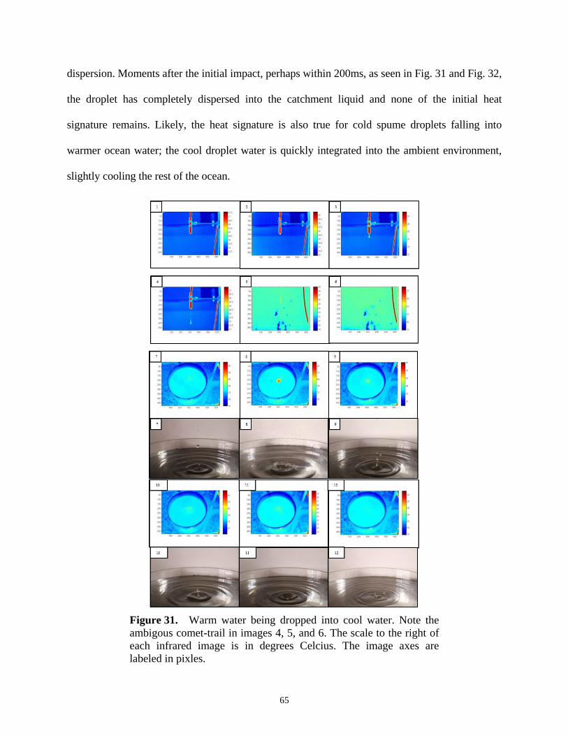
65
dispersion. Moments after the initial impact, perhaps within 200ms, as seen in Fig. 31 and Fig. 32,
the droplet has completely dispersed into the catchment liquid and none of the initial heat
signature remains. Likely, the heat signature is also true for cold spume droplets falling into
warmer ocean water; the cool droplet water is quickly integrated into the ambient environment,
slightly cooling the rest of the ocean.
Figure 31. Warm water being dropped into cool water. Note the
ambigous comet-trail in images 4, 5, and 6. The scale to the right of
each infrared image is in degrees Celcius. The image axes are
labeled in pixles.

66
Figure 32. Hot water being dropped into cold water. Note
the ambigous comet-trails are once again visible in images
1, 2, and 3. The scale to the right of each infrared image is in
degrees Celcius. The image axes are labeled in pixles.
d) Acoustic Power Spectra of Droplet Impacts
Six variations of drop height were used in the underwater acoustics experiment: 1.39m, 0.79m,
0.79m (again), 0.55m, 0.22m, and 0.09m. All the droplets were relatively large at about 6mm in
diameter. The hydrophone was integrated into an Olympus TG-1 point-and-shoot camera and thus
had right and left channels. The catchment tank was circular, 14.7cm in diameter, 30.5cm tall, and
was filled with 24.5cm of fresh water. The hydrophones were placed 15.5cm below the surface,

67
resting on a glass jar, directly underneath the droplet impact location. Water was dripped for some
time, between 30 seconds and two minutes, at rates of one drop per four seconds to one drop per
two seconds.
For the trials conducted at 0.55m and 0.09m drop height, the catchment tank was insulated
from floor vibrations by a large rubber pad set atop the insulated floor panel in the lab. For all
other trials the catchment tank was resting halfway on the insulated floor panel and halfway on
the regular floor panels, with only a wet rag between the tank and the floor. Figure 33 displays the
recorded volume of both channels of each trial.
Figure 33. Time distribution of signal power.
Trials A1 through A6 are of decreasing height from
1.39m, 0.79m, 0.79m (again), 0.55m, 0.22m, and
0.09m.
0 2 4 6 8
x 105
-1
0
1Left Channel Power
A1
0 2 4 6 8
x 105
-1
0
1Right Channel Power
0 2 4 6 8
x 105
-1
0
1
A2
0 2 4 6 8
x 105
-0.5
0
0.5
0 2 4 6 8
x 105
-0.5
0
0.5
A3
0 2 4 6 8
x 105
-0.5
0
0.5
0 2 4 6 8
x 105
-0.5
0
0.5
A4
0 2 4 6 8
x 105
-0.5
0
0.5
0 2 4 6 8
x 105
-1
0
1
A5
0 2 4 6 8
x 105
-0.5
0
0.5
0 2 4 6 8
x 105
-0.5
0
0.5
time steps
A6
0 2 4 6 8
x 105
-0.5
0
0.5
time steps

68
Three different frequency spectrum analysis methods were used to analyze the date; frequency
distribution of power, Fourier power spectrum, and power spectral density. Because the ambient
noise that was present while taking the acoustic measurements sounded more or less similar from
one trial to the next, no effort was made to filter the recordings. Figure 34 presents the frequency
distribution of power; specifically the volume of each frequency is plotted to show which
frequencies were loudest.
Figure 34. Frequency distribution of signal power. Trials A1
through A6 are of decreasing height from 1.39m, 0.79m, 0.79m
(again), 0.55m, 0.22m, and 0.09m.
0 2 4 6
x 104
-200
-100
0Left Channel Power
A1
0 2 4 6
x 104
-200
-100
0Right Channel Power
0 2 4 6
x 104
-200
-100
0
A2
0 2 4 6
x 104
-200
-100
0
0 2 4 6
x 104
-200
-100
0
A3
0 2 4 6
x 104
-200
-100
0
0 2 4 6
x 104
-200
-100
0
A4
0 2 4 6
x 104
-200
-100
0
0 2 4 6
x 104
-200
-100
0
A5
0 2 4 6
x 104
-200
-100
0
0 2 4 6
x 104
-200
-100
0
frequency
A6
0 2 4 6
x 104
-200
-100
0
frequency
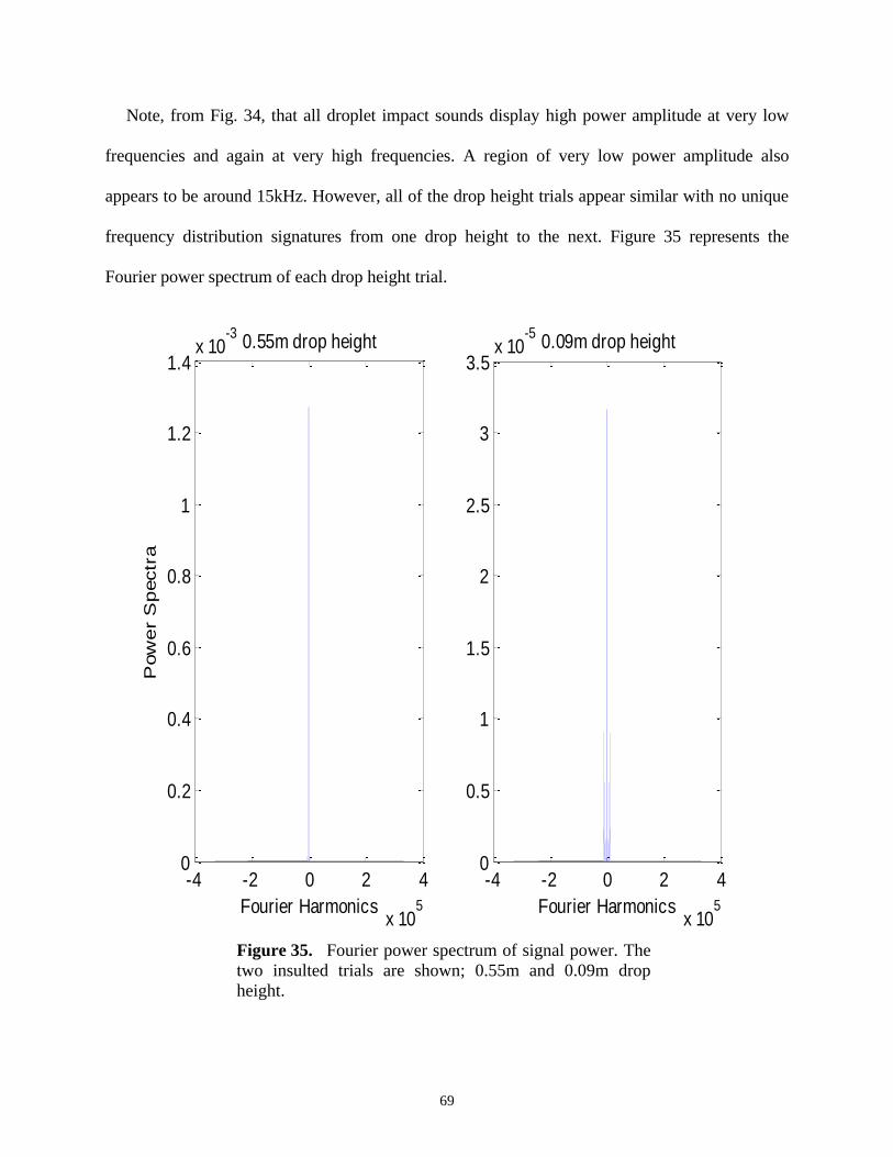
69
Note, from Fig. 34, that all droplet impact sounds display high power amplitude at very low
frequencies and again at very high frequencies. A region of very low power amplitude also
appears to be around 15kHz. However, all of the drop height trials appear similar with no unique
frequency distribution signatures from one drop height to the next. Figure 35 represents the
Fourier power spectrum of each drop height trial.
Figure 35. Fourier power spectrum of signal power. The
two insulted trials are shown; 0.55m and 0.09m drop
height.
-4 -2 0 2 4
x 105
0
0.5
1
1.5
2
2.5
3
3.5x 10
-50.09m drop height
Fourier Harmonics
-4 -2 0 2 4
x 105
0
0.2
0.4
0.6
0.8
1
1.2
1.4x 10
-30.55m drop height
Fourier Harmonics
Pow
er
Sp
ectr
a

70
Glancing at the plots, a primary harmonic may look to exist at a very low frequency and
common to all drop trials, and a secondary harmonic appears to grow with decreasing drop height.
However, as is clarified by Fig. 36, the secondary and tertiary harmonics are relatively stagnant
from one drop trial to the next, but the primary harmonic shrinks as the drop height decreases.
Figure 37 shows the spectral density of the signal power, which is a normalized version of the
frequency power distribution. Similar to the trend seen in Fig. 35 and Fig. 36, and the general
shape of Fig. 34, a pair of dominant frequencies, one at low frequencies and one at high
frequencies, appear exist, gradually decreasing in amplitude with decreasing drop height, thereby
allowing the secondary frequencies to stand out.
The biggest change from one drop height trial to the next appears to be in the amplitude of the
dominant frequency, which is relatively powerful at high drop heights, easily overwhelming any
secondary frequencies, but then tapers off as the drop height decreases.
Small rain drops, around 1mm in diameter, are known to produce high amplitude sound around
the spectral frequencies of 14 to 16kHz.[32], [33]
The most active spectral frequency in that range
seen in Fig. 37 is much lower than this, on the order of 1kHz; perhaps larger droplet produce
lower frequency impact acoustics. The next higher frequency with a power signature was around
500kHz; far too high to be comparable. The actual impact pulse only accounts for a small fraction
of the acoustic signature, and is not unique to droplet size or impact velocity.[33], [34]
The majority
of droplet impact acoustical power comes from bubble entrainment.[33], [34]
When the droplet hits the water surface, it punches a hole and creates a bubble. The
oscillations of this entrained bubble as it rises are the cause of most of the underwater sound
associated with droplet impacts.[33], [34]
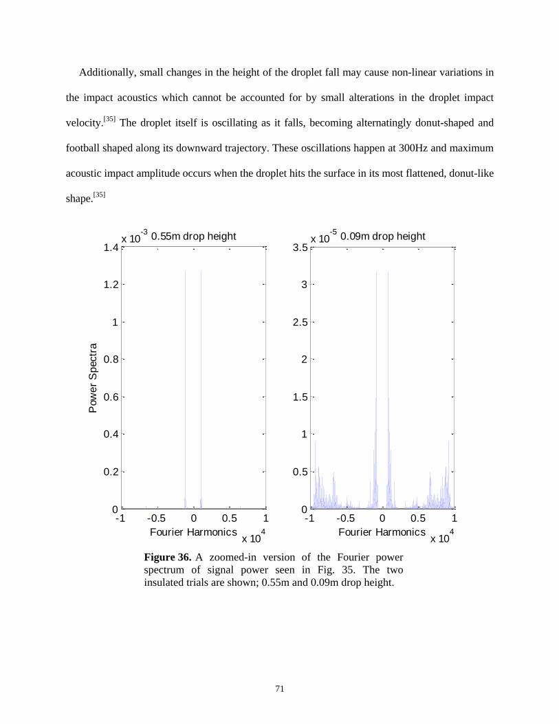
71
Additionally, small changes in the height of the droplet fall may cause non-linear variations in
the impact acoustics which cannot be accounted for by small alterations in the droplet impact
velocity.[35]
The droplet itself is oscillating as it falls, becoming alternatingly donut-shaped and
football shaped along its downward trajectory. These oscillations happen at 300Hz and maximum
acoustic impact amplitude occurs when the droplet hits the surface in its most flattened, donut-like
shape.[35]
Figure 36. A zoomed-in version of the Fourier power
spectrum of signal power seen in Fig. 35. The two
insulated trials are shown; 0.55m and 0.09m drop height.
-1 -0.5 0 0.5 1
x 104
0
0.5
1
1.5
2
2.5
3
3.5x 10
-50.09m drop height
Fourier Harmonics
-1 -0.5 0 0.5 1
x 104
0
0.2
0.4
0.6
0.8
1
1.2
1.4x 10
-30.55m drop height
Fourier Harmonics
Pow
er
Sp
ectr
a
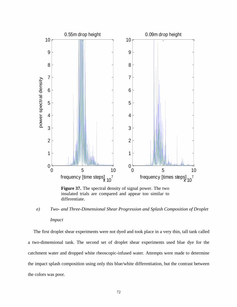
72
Figure 37. The spectral density of signal power. The two
insulated trials are compared and appear too similar to
differentiate.
e) Two- and Three-Dimensional Shear Progression and Splash Composition of Droplet
Impact
The first droplet shear experiments were not dyed and took place in a very thin, tall tank called
a two-dimensional tank. The second set of droplet shear experiments used blue dye for the
catchment water and dropped white rheoscopic-infused water. Attempts were made to determine
the impact splash composition using only this blue/white differentiation, but the contrast between
the colors was poor.
0 5 10
x 107
0
1
2
3
4
5
6
7
8
9
100.09m drop height
frequency [times steps]
0 5 10
x 107
0
1
2
3
4
5
6
7
8
9
100.55m drop height
frequency [time steps]
pow
er
sp
ectr
al d
ensit
y

73
In the third stage of droplet shear experiments, a shallow, wide tank called the three-
dimensional tank was used to catch, again, white drops falling into blue liquid. The fourth
experiment added red colored dye to the dropped rheoscopic solution, as seen in Fig. 38. From the
fourth experiment, the composition of the impact splash can be subjectively determined, and the
impact shear stresses are clearly visualized. Shutter and flash timing was refined using the
Arduino and changing the sensor position. Assuming the droplet impacts were more or less
identical from one splash to the next, a series of photos was taken during each phase of
experimentation to catch the droplets in various stages of fall and impact. To identify the source
of the surface shear striations seen in Fig. 38, the catchment fluid surface was stirred to disperse
any existing shear lines before allowing a droplet to impact thereby ensuring a quiescent surface.
Figure 38. The fourth rheoscopic fluid droplet experiment, allowing for clear visualization of
impact splash composition and impact shear stresses.

74
Figure 39 shows an impact splash as a white droplet of rheoscopic solution lands in the two-
dimensional catchment tank. Note how shallowly the droplet penetrates into the surface of the
rheoscopic solution. Droplet impact is entirely a surface phenomenon. The shear stresses seen in
Fig. 39 are generated by the addition of droplets to the top couple millimeters of water, and the
surface waves caused by the droplets. The splash transfers momentum, causing local surface
flows outward from the point of impact, which causes the growing shear boundary layer outward
from the splash.
As seen in Fig. 40, droplet impact causes a sub-surface bubble to form, not necessarily totally
entrained, as the impacting drop punches a hole in the surface. Then, several dozen milliseconds
later, this bubble collapses, generating the towering plume spike made famous by Edgerton's pink
milk photos. Droplet impact involves two parts: firstly; debris being thrown up around the site of
impact, and secondly; cavitation and collapse of a small air bubble resulting in a spray tower.
Figure 39. A droplet of white rheoscopic solution impacts with a two-
dimensional catchment reservoir of blue rheoscopic fluid. This image is
captured about 30ms after impact.

75
Darker lines in the liquid seen in Fig. 40, as well as all the other rheoscopic images, are areas
of shear stress aligned 90° from the surface of the liquid. Lighter areas are where the shear stress
runs along the surface plane. The fish scale flakes that which were added to make the liquid
rheoscopic align with the shear stresses. When seen face-on the flakes act as mirrors. When seen
edge on the flakes are nearly invisible and one can see deeper into the liquid (hence it looks
darker). Two shear modes of interest are present in Fig. 40: the vertical shear column directly
beneath the point of droplet impact caused by the impacting droplet pounding down a column of
water; and the shear ring around the expanding splash bubble as the water is stretched over the
expanding surface. Note the fractal-like vortices on the surface of the catchment liquid in Fig. 41.
No literature was found relating to this phenomenon.
Figure 40. Compilation of two-dimensional, white-on-white droplet impact of rheoscopic
fluid. Time sequence is from top left to lower right.

76
Figure 42 offers a closer look at the surface eddies, which appear after a single droplet impact,
then enlarge and shift after consecutive droplet impacts. These eddies only appear to affect the top
couple of millimeters of water, as evidenced by Fig. 39. Figure 43 demonstrates a hypothesized
cause of these surface eddies: secondary droplets impacting with the surface at an angle. Radial
impacts of secondary droplets would predict that the surface eddies are “cleanest” immediately
after the first drip onto a quiescent surface – that is, the surface eddies will be most clear. The
surface eddies should appear immediately after the first droplet impact. This collateral splash
droplet hypothesis does not hold up when Fig. 44 is considered. Here, a droplet can be seen
midair, milliseconds before impact, and very neat surface eddies are also visible below.
Obviously, these surface eddies persist and do not grow more complicated with consecutive
dropping, as one would expect from secondary droplet induced surface eddies.
Figure 41. Compilation of three-dimensional, white-into-blue droplet impact of rheoscopic
fluid. Time sequence is from top left to lower right.

77
Rather, the surface eddies are seen to expand with consecutive droplet impacts. Fig. 44 shows
an expanded eddy system. Additionally, the secondary splash-induced droplets, captured midair in
Fig. 45, are far too small to generate large surface eddies. The surface eddies are most likely due
to the surface waves generated by each droplet impact. When a droplet hits the surface, much of
its kinetic energy is transferred radially by sloshing the top few millimeters of surface water
outward. Notice the tiny secondary splash droplet being thrown into the air in Fig. 45 and Fig. 46.
These tiny droplets are much too small to generate the large surface eddies. Figure 45 through
Fig. 48 depict droplets of red dyed rheoscopic fluid falling onto a quiescent surface of blue dyed
liquid. Figure 45 through Fig. 50 are in time order of impact. Figure 45 does not show any surface
eddies prior to droplet impact. Instead a corona of blue liquid is being thrown up against a
perfectly featureless surface.
Figure 42. A closer look at the surface eddies of mysterious origin seen in Fig. 41.

78
In Fig. 46, meant to show an identical situation approximately 10 milliseconds after the scene
in Fig. 45, the first surface eddies can be seen forming within the expanding corona as the red
droplet begins to rebound, still intact. More secondary splash-induced droplets can be seen midair
in Fig. 46, as well. Clearly now, these secondary droplets are not the source of the surface shear
eddies. Figure 47 continues from Fig. 46; the original red droplet has rebounded yet further, and
the origin of the surface eddies is visible around the growing tower of blue liquid. The surface
eddies appear to be generated by shear forces in the expanding inner wall of the droplet impact
crater and then propagated outward by the “pumping” motion of the splash.
Figure 43. One possible cause of the surface eddies is hypothesized to be the impacts of
secondary droplets which were thrown up by the original droplet impact.
Hypothesized locations and
directions of secondary droplet
impact, causing eddies.
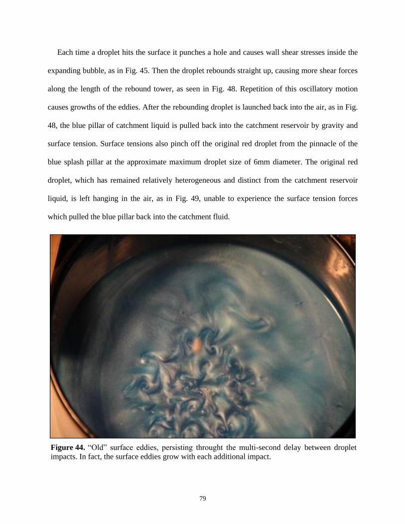
79
Each time a droplet hits the surface it punches a hole and causes wall shear stresses inside the
expanding bubble, as in Fig. 45. Then the droplet rebounds straight up, causing more shear forces
along the length of the rebound tower, as seen in Fig. 48. Repetition of this oscillatory motion
causes growths of the eddies. After the rebounding droplet is launched back into the air, as in Fig.
48, the blue pillar of catchment liquid is pulled back into the catchment reservoir by gravity and
surface tension. Surface tensions also pinch off the original red droplet from the pinnacle of the
blue splash pillar at the approximate maximum droplet size of 6mm diameter. The original red
droplet, which has remained relatively heterogeneous and distinct from the catchment reservoir
liquid, is left hanging in the air, as in Fig. 49, unable to experience the surface tension forces
which pulled the blue pillar back into the catchment fluid.
Figure 44. “Old” surface eddies, persisting throught the multi-second delay between droplet
impacts. In fact, the surface eddies grow with each additional impact.

80
Eventually, the red droplet falls back down due to gravity alone and creates a second impact
crater but does not rebound, mixing into the catchment liquid instead, as seen in Fig. 50. As to
whether the droplet impact splash is mostly catchment liquid or droplet liquid, the answer is: a
little of both. The impacting red spume droplet throws up a corona of warm blue water as it
punches a hole in the liquid surface. Then the spume droplet bounces back up, atop a tower of
warm water. The tower breaks apart, leaving the lonely spume droplet suspended midair. This
droplet is mostly made of the original spume water. In the ocean this midair spume would
evaporate more slowly than the splashed up seawater since it is colder than the seawater, but the
spume droplet would be left midair for longer.
Figure 45. Impact of a dyed red droplet into a dyed blue virgin surface. The outer ring is due to
stirring the fluid with a wooden stick.

81
B. Simulation of Unmanned Sailing
Sailing, in principal, is a balancing act between the hydrodynamic hull forces and the
aerodynamic sail forces. Achieving a force equilibrium in all but one degree of freedom is the
basic control goal.
a) Evaluation of Static Equilibrium Performance
Under steady-state sailing conditions, the ASV is not accelerating. That is, the forces acting on
the wing-sail and the keel are in equilibrium. To achieve this at constant sailing velocity, Vs, isn’t
too difficult, one must simply solve two sets of equations. But to analytically determine a
maximum Vs requires solving a non-linear model.
Figure 46. Moments after impact of a red-dyed droplet impacting a quiesent, blue surface, the
red droplet is rebounding.

82
The equations of the forces generated by each airfoil acting parallel and perpendicular to the
path of travel are shown in (22) as Fpara and Fperp , respectively. Both equations are functions of
the coefficients of lift and drag, CL and CD, and of the velocity of the ship, Vs. Coefficients CL and
CD are both functions of α;
𝐹𝑝𝑎𝑟𝑎 = ½𝜌𝑉𝐴2𝐴(𝐶𝐿 + 𝐶𝐷)1/2sin(𝛽– 𝜃) (22.1)
𝐹𝑝𝑒𝑟𝑝 = ½𝜌𝑉𝐴2𝐴(𝐶𝐿 + 𝐶𝐷)1/2cos(𝛽– 𝜃). (22.2)
To achieve equilibrium, three different sets of parameters must be balanced at once: first, the
wing sail pointing moment generated by the trim tab must match the wing sail pitching moment at
the given sail angle-of-attack and equilibrium apparent wind speed.
Figure 47. Continuing the rebound seen in Fig. 46, the red droplet begins to raise atop of pillar
of blue, catchment liquid.

83
Second, the keel pointing moment generated by the rudder must likewise match the keel
pitching moment at the equilibrium boat velocity and keel angle-of-attack. Thirdly, the lift and
drag forces generated by the keel-and-rudder combination must counteract those generated by the
wing-sail-and-trim tab combination at the equilibrium boat velocity and apparent wind speed.
The Matlab program created to find this balance is initialized by the user inputting the apparent
wind speed, the angle from which the wind is blowing with respect to the desired course of sail,
and the angle-of-attack made by the wing sail with the apparent wind. The angle-of-attack is user-
generated to remove one layer of complexity from the program. The optimal angle-of-attack for a
wide range of apparent wind speeds can be approximated as 11.5 degrees. This optimal angle was
arrived at after a series of simulations to model the wing sail response to different wind speeds.
Figure 48. At its maximum secondary height, the red droplet which initially caused the splash
has rebounded atop a pillar of blue catchment water. The red droplet has remained
hetergeneously unmixed with the blue liquid.

84
Approximating the angle-of-attack allows one layer of iterative loops to be removed. When
sailing the hypothetical sailing spar on a real ocean, optimizing the angle of attack at every time
step will likely be too compuatationally burdensome and a generally acceptable value will be
chosen instead – as done for these simulations.
Since the wing sail angle-of-attack is user defined and generally chosen to be 11.5 degrees, the
trim tab pointing angle can be calculated. Then the remaining parameters of rudder pointing
angle, keel angle-of-attack, and boat velocity must be simultaneously balanced. The Matlab script
does so using a series of nested loops. Pitching and heeling angles follow once the previous three
parameters are determined.
Figure 49. Having been pulled back flat into the liquid by surface tensions, the blue tower has
left the original red droplet hanging midair.

85
The Matlab script uses embedded loops to numerically determine the equilibrium values of
each parameter, and due to loop sizes, the counteracting forces generally do not match perfectly
due to the loop step sizes. Therefore, the user is also prompted to set the resolution of the
simulation; that is, the step size of the nested loops determines the accuracy of the results – the
size of the acceptable equilibrium window. Additionally, the Matlab simulation makes the
following, simplifying assumptions about the world:
- The sea surface is flat.
- Despite the calculated pitching and heeling angles, the sailing spar remains perfectly
vertical as far as the aerodynamic forces are concerned.
- The wind blows smooth and gustless.
- The airfoil surfaces are frictionless.
- No turbulence is present in the air or water
- The airfoils behave as infinite wings with no wingtip vortices or other low aspect ratio
phenomenon.
- No measurement or instrumentation error or noise is present.
- The trim tab strut arms and sail-keel pivot joint do not affect the aerodynamics.
- Equilibrium conditions are considered steady state.
In generating Fig. 51 through Fig. 53 the program limited the apparent wind direction range to
between 20 and 100 degrees apparent wind direction; 20 degrees being the maximum upwind
reach below which the keel stalls, and 100 degrees being the maximum downwind run above
which a parachute configuration is more effective. Figure 51 predicts the maximum achievable
velocity of the ASV in ideal conditions to be about 2.6 knots at 65 degrees apparent wind. Friction
drag would certainly reduce the maximum predicted spar velocity. Friction drag may also shift the
apparent wind angle at which the maximum velocity occurs, since close reaches will suffer higher
drag opposing the boat’s forward motion, while shallow, beam reaches will not be subjected to
the same drag – only a stronger heeling force.

86
Figure 50. The red droplet follows the blue tower back into the catchment liquid, leaving a
small indent from its secondary impact.
In Fig. 52 leeway angle – or, keel angle-of-attack – describes the side slip of the boat
downwind through the water. Again, because of friction drag, both the keel and wing-sail airfoils
are expected to feature lower efficiencies in reality, resulting in greater keel side slippage.
The trends seen in Fig. 53 show that maximum pitching occurs at the predicted maximum
velocity, and maximum heeling occurs at the steepest upwind haul. An obvious prediction from
Fig. 53 is that the maximum heeling angle will be nearly two degrees greater than the maximum
pitching angle of the ASV, at a true wind of 10 knots. This result is as expected, since
conventional sailboats also heel much more than they pitch when under sail. Table 2 tabulates the
equilibrium outputs from one iteration of the Matlab simulation. Note the small heeling and
pitching angles compared to a conventional sailboat in similar conditions.[18]

87
For engineering reaffirmation and to run computational fluid dynamics (CFD) simulations the
sailing spar was modeled using SolidWorks drafting software, the results of which modeling are
shown in Fig. 54 and Fig. 55. The sailing spar modeling was done in such a way that each airfoil
component could be individually set at a chord-wise angle relative to the other components.
Different equilibrium configurations could thus be simulated in the SolidWorks proprietary CFD
ad-on. A screen shot of one wing sail configuration simulation result is shown in Fig. 54. The
SolidWorks CFD simulations had most of the same simplifying assumptions as the Matlab
simulations except for the following:
- The airfoil surfaces do have friction.
- Turbulence is simulated.
- The airfoils do behave as finite wings.
- The strut arms and wing-keel pivot joint do influence the aerodynamics.
Figure 51. Equilibrium spar velocity given the direction from which the apparent
wind is coming, at a true wind of 10 knots.
0
0.5
1
1.5
2
2.5
3
0 20 40 60 80 100 120
Pre
dic
ted
Sp
ar
Ve
loci
ty [
kn
ots
]
Apparent Wind Angle [deg]
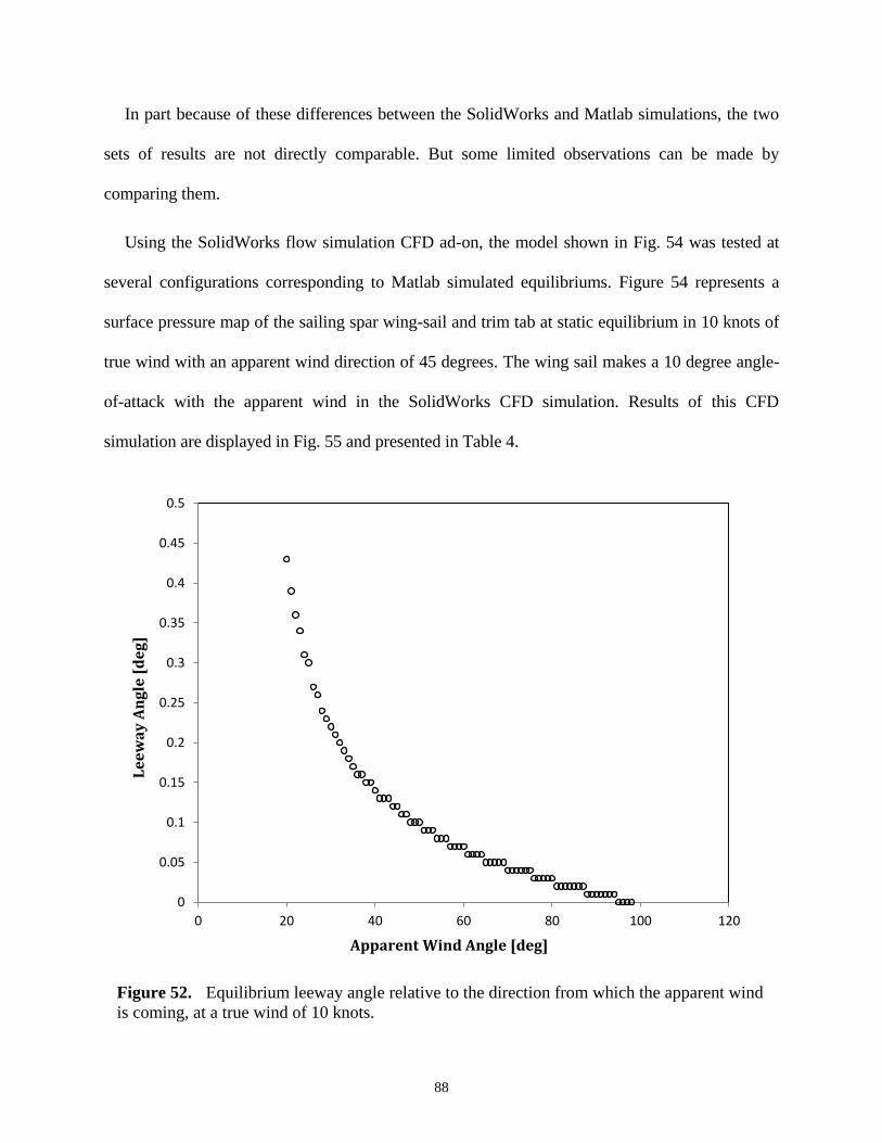
88
In part because of these differences between the SolidWorks and Matlab simulations, the two
sets of results are not directly comparable. But some limited observations can be made by
comparing them.
Using the SolidWorks flow simulation CFD ad-on, the model shown in Fig. 54 was tested at
several configurations corresponding to Matlab simulated equilibriums. Figure 54 represents a
surface pressure map of the sailing spar wing-sail and trim tab at static equilibrium in 10 knots of
true wind with an apparent wind direction of 45 degrees. The wing sail makes a 10 degree angle-
of-attack with the apparent wind in the SolidWorks CFD simulation. Results of this CFD
simulation are displayed in Fig. 55 and presented in Table 4.
Figure 52. Equilibrium leeway angle relative to the direction from which the apparent wind
is coming, at a true wind of 10 knots.
0
0.05
0.1
0.15
0.2
0.25
0.3
0.35
0.4
0.45
0.5
0 20 40 60 80 100 120
Le
ew
ay
An
gle
[d
eg
]
Apparent Wind Angle [deg]
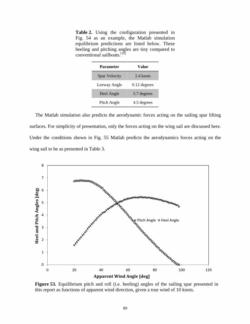
89
Table 2. Using the configuration presented in
Fig. 54 as an example, the Matlab simulation
equilibrium predictions are listed below. These
heeling and pitching angles are tiny compared to
conventional sailboats.[18]
Parameter Value
Spar Velocity 2.4 knots
Leeway Angle 0.12 degrees
Heel Angle 5.7 degrees
Pitch Angle 4.5 degrees
The Matlab simulation also predicts the aerodynamic forces acting on the sailing spar lifting
surfaces. For simplicity of presentation, only the forces acting on the wing sail are discussed here.
Under the conditions shown in Fig. 55 Matlab predicts the aerodynamics forces acting on the
wing sail to be as presented in Table 3.
Figure 53. Equilibrium pitch and roll (i.e. heeling) angles of the sailing spar presented in
this report as functions of apparent wind direction, given a true wind of 10 knots.
0
1
2
3
4
5
6
7
8
0 20 40 60 80 100 120
He
el
an
d P
itch
An
gle
s [d
eg
]
Apparent Wind Angle [deg]
Pitch Angle Heel Angle

90
Table 3. The Matlab simulation predictions for the wing-
sail static equilibrium in 10 knots of true wind with an
apparent wind direction of 45 degrees. The wing sail makes
a 10 degree angle-of-attack with the apparent wind.
MA
TL
AB
Parameter Value
Lifting Force 20.6 Newtons
Drag Force 2.5 Newtons
Pitching Moment 0 Newton-meters
SolidWorks predicts vastly different aerodynamic forces than the Matlab equilibrium solutions.
The SolidWorks numbers don’t even achieve pitching equilibrium in the wing sail. The
SolidWorks simulation results, which include friction drag, are presented in Table 4 for the
configuration seen in Fig. 55.
Figure 54. Graphic results of a SolidWorks CFD simulation
showing pressure distribution across a wing sail set to an
equilibrium configuration found using Matlab. Here, the angle-of-
attack is 10 degrees to the apparent wind which is blowing at 45
degrees from the sailing trajectory of the spar at 10 knots.

91
Table 4. The SolidWorks simulation predictions for the wing-sail
static equilibrium in 10 knots of true wind with an apparent wind
direction of 45 degrees. The wing sail makes a 10 degree angle-of-
attack with the apparent wind.
SO
LID
WO
RK
S
Parameter Value
Lifting Force 5.4 Newtons
Drag Force 1.5 Newtons
Pitching Moment 4.6 Newton-meters
Using the noise and bias described in (9) and (10) and the aerodynamic relationships of (4) and
(5), and (11) through (13) simulated measurements were made of the apparent wind velocity. Data
were collected at a rate of 10 Hertz for a full minute. The prevailing winds were simulated to be
blowing at 10 knots, or 5.14 meters per seconds, from 10 degrees off the sailed course. These
values are given relative to the ASV’s reference.
Figure 55. SolidWorks flow simulation results. The goals of the solver
were to find the aerodynamic forces acting on the wingsail.

92
b) Filtering of Sensor Noise
The sensors which detect wind velocity produce noise, which makes navigation more difficult.
Since much of the noise is inherently random, no two simulations look much alike. Therefore,
from one figure to the next, data may be different. What matters are the relationships within each
figure. Figure 56 presents the wind speed data from the minute long simulation. Note that the true
wind speed – set, as mentioned above, at 5.14 m/s – is never reported by the sensor; the vortex
bias is simply too strong at this wind speed. Sail behavior shows a slight vortex effect as well.
Figure 56. Simulated wind speed measurements are
compared to the wind felt by the wing-sail sensor and to the
actual apparent wind reaching the ASV.
Much like in Fig. 56 the data shown in Fig. 57 demonstrates a bias in the simulated wing-sail-
top measurements. The actual lower-frequency response of the wing-sail is overlaid showing that,
notwithstanding the bias, the data measured by the sensor is flawed and reports a higher-
frequency noise relative wind direction fluctuations which do not affect the behavior of the wing-
sail.
0 10 20 30 40 50 605.1
5.2
5.3
5.4
5.5
5.6
5.7
5.8
5.9
seconds
m/s
Wind Speed
nominal
as governs wingsail behavior
as reported by sensor

93
For the wing-sail mounted weather sensors, the noise is neither Gaussian nor zero-mean. There
is a bias due to vortices generated at the top of the wing-sail. This bias is significant at lower wind
speeds, like the speed simulated. Additionally, the distribution of the noise in each term of the
rolling motion series is constant.
Figure 57. Simulated wind direction measurements are
compared to the wind felt by the wing-sail and to the nominal
apparent wind.
Due to the numerous terms in this series, the noise may be approaching a more Gaussian-like
distribution. However, it will be considered to be of constant distribution. The noise is
uncorrelated; since the ocean is so vast, the ASV cannot affect it.
The noise in the servo-motor sensors is a different story from the weather sensor noise. Figure
58 demonstrates different methodologies – noisy and true – for calculating the pitching moment
of the wing-sail. The noise in the servo-motor sensors is both Gaussian and zero-mean; it is due
only to the sensors themselves.
0 10 20 30 40 50 607
8
9
10
11
12
13
14
15
16
seconds
deg
rees
Wind Direction
nominal
as governs wingsail behavior
as reported by sensor

94
In Fig. 58, the nominal and true pitching moments are shown. In should be noted that the true
pointing moment generated by the trim tab does match the true pitching moment of the wing-sail.
This is because δ is held constant in this simulation, set to counter the nominal pitching moment.
Figure 58. The true wing-sail pitching moment, as a function of the
low-frequency rolling motion responded to by the wing-sail, is
compared to the predicted pitching and pointing moments. Predictions
are based on mast top weather sensors and the trim tab torque
measurements. The nominal, roll-free pitching moment is also shown.
But since the trim tab pointing moment is a function of α to a different degree than is the
pitching moment of the wing-sail, at an oscillating angle-of-attack the wing-sail pitch will lag the
presented “true” α. Both methods used to filter the noisy data were based on discrete
measurements; a continuous-discrete Extended Kalman Filter and a discrete Linear Kalman
Filter.[36]
Since the ASV will presumably be using a computer, all the measurements will made
discretely (chosen at 10 Hz for the simulation) but the system itself is continuous. Therefore, both
continuous-discrete and discrete-discrete filters can be used.
0 10 20 30 40 50 60-0.1
-0.05
0
0.05
0.1
0.15
0.2
0.25
0.3
0.35
seconds
N-m
Nominal, True, and Predicted Pitching and Pointing Moments
Nominal Wingsail Pitching Moment
True Wingsail Pitching Moment
Wingsail Pitching Moment Predicted from Mast-Top Sensors
Trimtab Pointing Moment Predicted from Mast-Top Sensors
Trimtab Pointing Moment Predicted incorporating Measured Trimtab Torque

95
Furthermore, the bias inherent in the weather sensors is removed heuristically – this is not
unreasonable and is explained below. The servo-motor data is additionally filtered with a moving
average as well as an overall average. The results of all four filtering methods are presented.
(1) Extended Kalman Filter with Bias Removal
The non-linearity of the weather-sensor noise seemed best filtered by an Extended Kalman
Filter, despite the biased noise. Using Table 5 as a guide, estimates for both the wind speed, VA,
and the wind direction, α, were generated. The model was generated using a constant value for the
true VA and α, meaning �̇� in Table 5 was zero. The measurements were taken from the simulated
noisy VA and α. To create the Hk function, the derivative of the noise series was painstakingly
found and used in the Gain calculations. Because the derivatives of both the wind speed and wind
direction were set to zero, propagation required simply transferring the updated value to the
beginning of the loop. However, it seems likely that this method is not ideal since the true VA and
α are not constant but fluctuate with the low-frequency motion of the wing-sail.
Table 5. The basic method for implementing an Extended Kalman Filter.[36]

96
Bias removal is achieved after the Extended Kalman Filter results were ascertained. The
estimate for the wind speed was about twice again as far from the true value as the noisy
measurements are in Fig. 59. The difference is then subtracted and a reasonable estimate is
produced. This deus ex machina manipulation is reasonable since a tried and true filtering system
will have had known biases removed heuristically through trial and error.
Running the first, continuous-discrete non-linear filter produced the results of Fig. 59. It was
noted that the estimate appeared to be almost exactly twice the measurement bias from the true
wind speed.
Figure 59. Using the Extended Kalman Filter to estimate the wind
speed produced results with an error nearly twice the bias.
0 10 20 30 40 50 605.1
5.2
5.3
5.4
5.5
5.6
5.7
5.8
5.9
6
6.1
seconds
m/s
Wind Speed Estimate versus Measurement
Nominal
True
Measured
EKF estimate
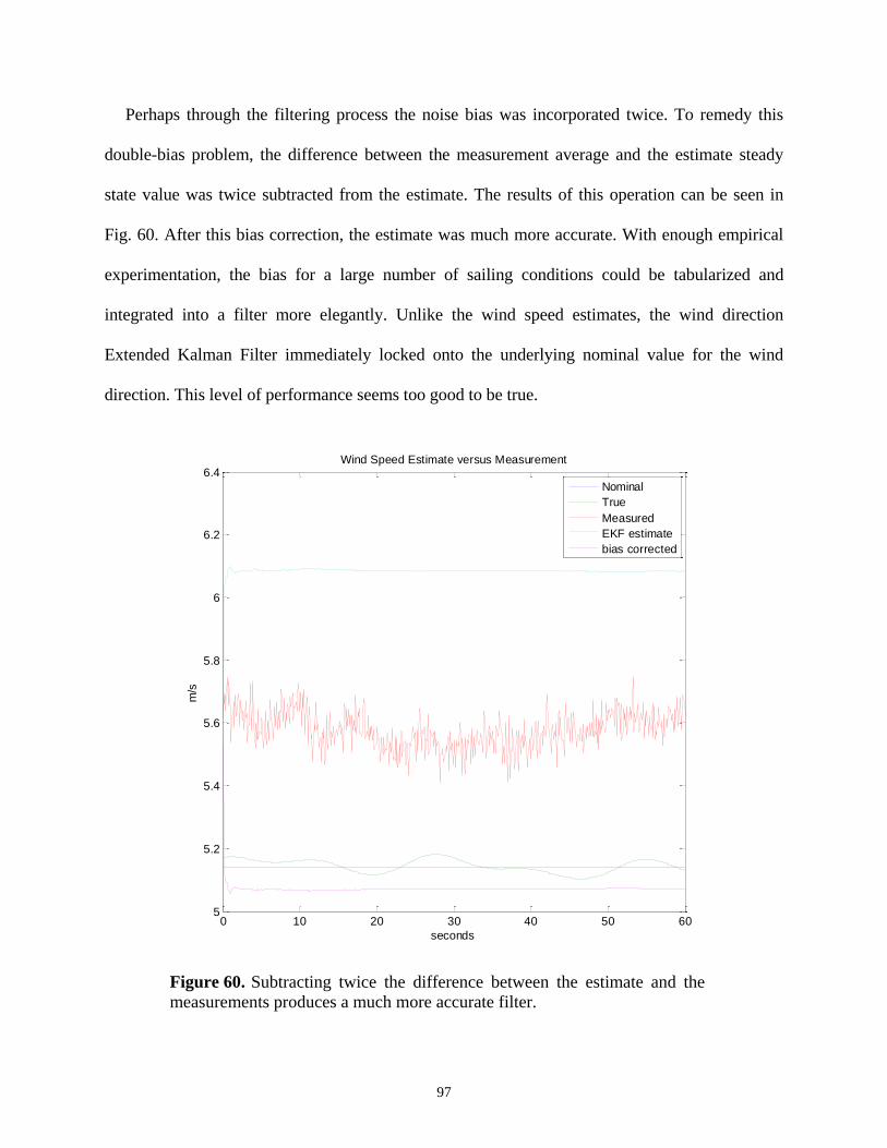
97
Perhaps through the filtering process the noise bias was incorporated twice. To remedy this
double-bias problem, the difference between the measurement average and the estimate steady
state value was twice subtracted from the estimate. The results of this operation can be seen in
Fig. 60. After this bias correction, the estimate was much more accurate. With enough empirical
experimentation, the bias for a large number of sailing conditions could be tabularized and
integrated into a filter more elegantly. Unlike the wind speed estimates, the wind direction
Extended Kalman Filter immediately locked onto the underlying nominal value for the wind
direction. This level of performance seems too good to be true.
Figure 60. Subtracting twice the difference between the estimate and the
measurements produces a much more accurate filter.
0 10 20 30 40 50 605
5.2
5.4
5.6
5.8
6
6.2
6.4
seconds
m/s
Wind Speed Estimate versus Measurement
Nominal
True
Measured
EKF estimate
bias corrected

98
Figure 61. Although the measurements to not appear to contain any
hint of the true values to the naked eye, the Extended Kalman Filter is
successful in locking onto the underlying nominal wind direction.
It is suspected that because the Extended Kalman Filter uses a constant value for its truth
model, and a value of null for the truth derivative, the estimate for the wind direction was
unrealistically able to track the nominal value.
This “perfect tracking” behavior is demonstrated in Fig. 61. Because the filter was using an
exact derivative of the noise, it was simple to cancel out the noise, including the low-frequency
rolling, leaving only the nominal wind direction value.
(2) Discrete Linear Kalman Filter
After the disappointing performance of the Extended Kalman Filter and the irrevocably biased
noise in the weather sensors, the zero-mean, Gaussian noise of the servo-motor sensors seemed
appealing. From (11), and using the more acceptably Extended Kalman Filtered α it is possible to
0 10 20 30 40 50 607
8
9
10
11
12
13
14
15
degrees from course
deg
ree
s
Wind Direction Estimate versus Measurement
Nominal
True
Measured
EKF estimate

99
back out a VA2 term from the measured torque, Mt, and position, δ, of the trim tab servo-motor.
This calculation leaves the wind speed term linear dependent on the measured wind direction, trim
tab position, and trim tab pitching moment.
Table 6. The basic method for implementing a
Discrete Linear Kalman Filter.[36]
However, although the noise in the servo-motor sensors is the same magnitude as that
generated within the weather sensors themselves, the torque required by the servo-motor is
miniscule at the conditions presented in the simulation. The noise of the servo-motor sensors
drowned out the signal and made process impossible. Since the noise in the servo-motor sensors is
known to be zero-mean Gaussian, it was believed that by averaging the measurements, first in a
moving window, then over the entire data set, the true wind speed could be calculated from (11).
However, certain measurements, either from the wind direction noise or the servo-motor sensor
noise, cause giant and unpredictable fluctuations in the average. To avoid dealing with the bias in
the weather sensor data, the plan was to collect only the unbiased wind direction estimates of Fig.
61 (presuming the filter hadn’t cheated) and, using (11) and the noisy servo-motor sensor
measurements, calculate a more accurate, unbiased wind speed estimate. Figure 62 presents just
that procedure: filtered α and unfiltered servo-motor measurements.

100
Figure 62. Using (3) and the filtered wind direction data of Fig. 61, an
estimate for the wind speed is presented using raw servo-motor
measurements for Mt and δ in the calculations.
Clearly, occasional stochastic excitation of a resonance is causing enormous jumps in the
calculations of VA2 using raw servo-motor data. The random noise is likely interfering
constructively by chance at certain times and the calculations used to find the estimated wind
speed may amplify these signals.
Since VA2 is a linear function of the other three measurements, it was presumed that a purely
discrete, linear Kalman Filter would remove the chance anomalies in the estimate of wind speed.
Using the discrete linear Kalman Filter of Table 6 the results of Fig. 63 were produced.
0 10 20 30 40 50 60-1
-0.5
0
0.5
1
1.5
2x 10
6
seconds
m2/s
2
Squared Wind Speed from Trim Tab Sensors
trim tab sensors
nominal
true
wing-tip sensor
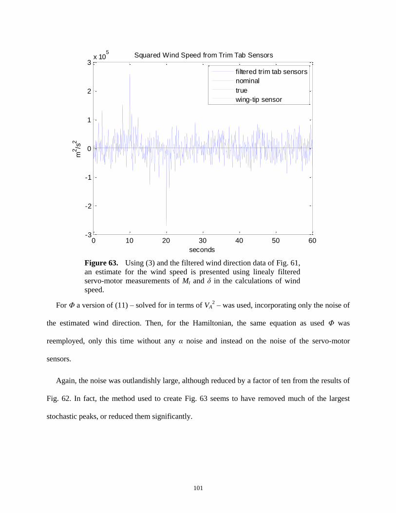
101
Figure 63. Using (3) and the filtered wind direction data of Fig. 61,
an estimate for the wind speed is presented using linealy filtered
servo-motor measurements of Mt and δ in the calculations of wind
speed.
For Φ a version of (11) – solved for in terms of VA2 – was used, incorporating only the noise of
the estimated wind direction. Then, for the Hamiltonian, the same equation as used Φ was
reemployed, only this time without any α noise and instead on the noise of the servo-motor
sensors.
Again, the noise was outlandishly large, although reduced by a factor of ten from the results of
Fig. 62. In fact, the method used to create Fig. 63 seems to have removed much of the largest
stochastic peaks, or reduced them significantly.
0 10 20 30 40 50 60-3
-2
-1
0
1
2
3x 10
5
seconds
m2/s
2
Squared Wind Speed from Trim Tab Sensors
filtered trim tab sensors
nominal
true
wing-tip sensor

102
(3) Moving Average Filter
Out of frustration with the self-imposed challenging noise, simple averaging was tried.
The raw servo-motor sensor data was averaged, first with a moving window of one second in
length, and then an overall average was used to find the mean of the entire data set of both servo-
motor sensors.
Figure 64. Averaging the raw servo-motor sensor data in a moving
window of 10 time steps produces slightly better results, but still terrible.
Figure 64 shows the moving window average while Fig. 65 shows the overall average. Both
averages were combined with the estimated wind direction.
Neither averaging method worked very well. The data in Fig. 64 is comparable to that of Fig.
63, which doesn’t make the linear Kalman Filter look good. Although still a terrible estimate, the
overall average produces the best results for the servo-motor data.
0 10 20 30 40 50 60-18
-16
-14
-12
-10
-8
-6
-4
-2
0
2x 10
5
seconds
m2/s
2
Squared Wind Speed from Trim Tab Sensors
averaged trim tab sensors
nominal
true
wing-tip sensor

103
c) Identification of System Control Process
After the sailing spar equilibrium model was condensed into a SISO system, the Matlab
System Identification Toolbox was used to estimate an ARMAX model, a transfer function
model, and a state space model.
Figure 65. Simply averaging all of the raw servo-motor direction and
torque measurements before using them to calculate the estimated wind
speed produces the best results. This is a pretty rough-shod filter.
The ARMAX model took the form of (23.1), the transfer function model followed (23.2), and
the state space model adopted the form seen in (23.3) and (23.4);
𝐴(𝑞)𝑦(𝑡) = 𝐵(𝑞)𝑢(𝑡 – 𝑛𝑘) + 𝐶(𝑞)𝑒(𝑡) (23.1)
𝐻(𝑠) = 𝐵(𝑠)/𝐴(𝑠) (23.2)
𝑥’(𝑡) = 𝐴𝑥(𝑡) + 𝐵𝑢(𝑡) + 𝐾𝑒(𝑡) (23.3)
𝑦(𝑡) = 𝐶𝑥(𝑡) + 𝐷𝑢(𝑡) + 𝑒(𝑡). (23.4)
0 10 20 30 40 50 60-500
-400
-300
-200
-100
0
100
200
300
400
500
seconds
m2/s
2
Squared Wind Speed from Trim Tab Sensors
overall averaged trim tab sensors
nominal
true
wing-tip sensor

104
All three models were initiated with a fixed number of free parameters. The ARMAX model
parameters, A, B, and C were of 3rd
, 2nd
, and 1st order, respectively, with zero time delay. The
transfer function had three poles and two zeros. And the state space model was third order
(occasionally, 3rd
order would become unstable and the state space model would be heuristically
reduced to second or first order). The ideal number of free parameters was found experimentally,
through trial and error. After the input and output vectors were objectified using the Matlab
command iddata, the commands armax, tfest, and ssest were used to generate their
respective models. This process was run iteratively; the output vector gained one data point after
each successive iteration. As long as the output vector was shorter than about twenty indices, the
data objectification command would not function and no system identification was possible until
an identifiable trend was established.
Figure 66. The true boat velocity, with noise, is compared to each
of the three iterative estimations and the three final estimations. The
iterative ARMAX model is not simulated in this plot due to unreliable
response behavior including the oft appearance of singularities.
0 5 10 15 20 25-2
-1
0
1
2
3
4
Seconds
mete
rs p
er
se
con
d
System Identification Methods
True Boat Speed
Final ARMAX
Iterative Transfer Function
Final Transfer Function
Iterative State Space
Final State Space
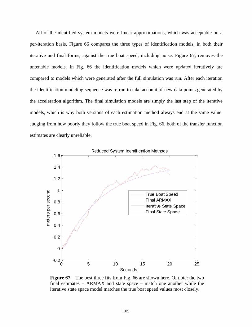
105
All of the identified system models were linear approximations, which was acceptable on a
per-iteration basis. Figure 66 compares the three types of identification models, in both their
iterative and final forms, against the true boat speed, including noise. Figure 67, removes the
untenable models. In Fig. 66 the identification models which were updated iteratively are
compared to models which were generated after the full simulation was run. After each iteration
the identification modeling sequence was re-run to take account of new data points generated by
the acceleration algorithm. The final simulation models are simply the last step of the iterative
models, which is why both versions of each estimation method always end at the same value.
Judging from how poorly they follow the true boat speed in Fig. 66, both of the transfer function
estimates are clearly unreliable.
Figure 67. The best three fits from Fig. 66 are shown here. Of note: the two
final estimates – ARMAX and state space – match one another while the
iterative state space model matches the true boat speed values most closely.
0 5 10 15 20 25-0.2
0
0.2
0.4
0.6
0.8
1
1.2
1.4
1.6
Seconds
mete
rs p
er
se
con
d
Reduced System Identification Methods
True Boat Speed
Final ARMAX
Iterative State Space
Final State Space

106
Figure 67 demonstrates that out of the top three estimation methods, the iterative state space
model most closely resembles the true boat speed behavior. The state space model shown in Fig.
66 and Fig. 67 happens to be first order. The time steps between iterations of the velocity
prediction program were usually set to somewhere between 0.001 seconds and 1 second, most
often 0.1 seconds. One tenth of a second step time was chosen as a balance between accuracy and
computation time. Running the full velocity prediction, system identification, and adaptive control
program with a time step of 0.1 seconds for 200 iterations took around fifteen to twenty minutes.
Larger time steps would generate unreliable results in the force balance solver.
Depending on how the simulation was initialized and what suggested course the wind angle
took, all of the identified system models were over 97% accurate, despite the nonlinearities
introduced by the wind angle constraints. This high level of accuracy seems to belie the clearly
incorrect estimates seen in Fig. 66. Heuristically choosing the best fit estimate was most practical.
Figure 68. The iterative linear model generator uses the Matlab System
Identification Toolbox to estimate a state space model of the velocity
prediction algorithm from the inputs and outputs. The adaptive feedback
controller uses a greedy method to compare how one-step-ahead variations
in the input vector would affect the outputs, then chooses the variation
which maximizes velocity in the next step.

107
For the adaptive controller, the state space model was chosen to provide the system
identification and was used to calculate feedback adjustments. A first order state space model was
also used to model the acceleration relationship. Figure 68 represents the system identification
and adaptive controllers as additions to the block diagram seen in Fig. 28. Noisy input data and
noisy output data are collected and fed into the system identifier, which then generates a linear
approximation of the relationship between the input angle and the boat speed. The system
identifier has access to the full set of input wind angles, since the route is planned. However, the
boat speed is known only up to the most recent step. This forces the identifier to update after
consecutive iterations before feeding the new model to the adaptive controller. Additionally, the
changes made to the input vector by the adaptive controller offer another reason to update the
system identifier after each iteration to take account of the new set of inputs and outputs.
Figure 69. One-step-ahead greedy adjustments of ±0.3 degrees to
the wind direction based on velocity maximization. The performance
does not increase significantly when using this adaptive controller.
0 5 10 15 20 250
20
40
60
80
100
120
140
Input-Output
time [seconds]
Tru
e W
ind A
ngle
[ d
eg ]
True Wind Speed and Acceleration Time V
t = 5.14 [m/s]
t( 95% ) = 12.1 [seconds]
True Wind Angle (input)
Boat Speed (output)
0 5 10 15 20 25-1
0
1
2
Boa
t S
pe
ed
[ m
/s ]

108
d) Adaptively Controlling the System
Three control methods were used to minimize the predicted velocity settling time: a one-step-
ahead greedy method which maximized velocity or acceleration at each iteration variation, a full-
time simulator which chooses the best of three slight variations on the full set of wind direction
inputs, and a heuristically optimized version of the impulse-step function used to describe the
wind direction. The one-step-ahead greedy controller used the estimated system model to
extrapolate the input-output relationship one step into the future. Then the input wind angle of the
one-step-ahead extrapolation was both increased and decreased slightly and the predicted boat
speeds estimated by these variations were compared.
Figure 70. Much like the controller of Fig. 69, here one-step-ahead greedy
adjustments of ±0.3 degrees to the wind direction are made based on acceleration
maximization. The performance improves somewhat when using this adaptive
controller. However, the one-step-ahead method violates wind direction constraints
established through initialization.
0 5 10 15 20 250
20
40
60
80
100
120
Input-Output
time [seconds]
Tru
e W
ind A
ngle
[ d
eg ]
True Wind Speed and Acceleration Time V
t = 5.14 [m/s]
t( 95% ) = 9.8 [seconds]
True Wind Angle (input)
Boat Speed (output)
0 5 10 15 20 25-1
0
1
2
Boa
t S
pe
ed
[ m
/s ]
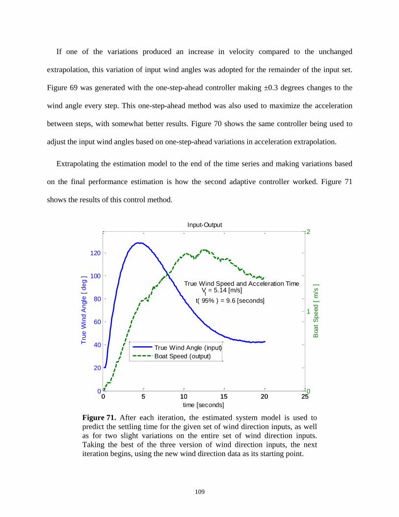
109
If one of the variations produced an increase in velocity compared to the unchanged
extrapolation, this variation of input wind angles was adopted for the remainder of the input set.
Figure 69 was generated with the one-step-ahead controller making ±0.3 degrees changes to the
wind angle every step. This one-step-ahead method was also used to maximize the acceleration
between steps, with somewhat better results. Figure 70 shows the same controller being used to
adjust the input wind angles based on one-step-ahead variations in acceleration extrapolation.
Extrapolating the estimation model to the end of the time series and making variations based
on the final performance estimation is how the second adaptive controller worked. Figure 71
shows the results of this control method.
Figure 71. After each iteration, the estimated system model is used to
predict the settling time for the given set of wind direction inputs, as well
as for two slight variations on the entire set of wind direction inputs.
Taking the best of the three version of wind direction inputs, the next
iteration begins, using the new wind direction data as its starting point.
0 5 10 15 20 250
20
40
60
80
100
120
Input-Output
time [seconds]
Tru
e W
ind A
ngle
[ d
eg ]
True Wind Speed and Acceleration Time V
t = 5.14 [m/s]
t( 95% ) = 9.6 [seconds]
True Wind Angle (input)
Boat Speed (output)
0 5 10 15 20 250
1
2
Boa
t S
pe
ed
[ m
/s ]

110
Using the full time series extrapolation seen in Fig. 71 the controller chooses the variation that
produces the shortest settling time. All subsequent input vector values would then be changed to
account for this variation. The full time series estimation controller used the same wind angle
variations as the one-step-ahead greedy method, ±0.3 degrees. Unlike the greedy method, the full
time series extrapolation method does not disregard the wind angle constraints. Because of the
unimpressive nature of the adaptive controller results, an attempt was made to tune the input wind
direction vector by hand. Noting the performance improvements suggested by the adaptive
controllers, the wind direction was modeled as a combination of an impulse response and a step
response of a second order damped system.
Figure 72. Adding an impulse to the function that generates the changing
wind direction angle greatly decreases the settling time. An impulse
response allows the boat to swing completely downwind to maximize
acceleration before quickly turning upwind, again, to the desired tack. The
impulse-step response can be hand-tuned to minimize settling time by
varying the impulse magnitude (how steeply the boat turns downwind
before turning back upwind), the natural frequency (how sharply the boat
turns), and the damping ratio (how closely the boat trajectory follows the
desired tack).
0 5 10 15 20 250
20
40
60
80
100
120
140
160
180
Input-Output
time [seconds]
Tru
e W
ind A
ngle
[ d
eg ]
True Wind Speed and Acceleration Time V
t = 5.14 [m/s]
t( 95% ) = 6.9 [seconds]
True Wind Angle (input)
Boat Speed (output)
0 5 10 15 20 25-2
0
2
Boa
t S
pe
ed
[ m
/s ]

111
Tuning was done by varying the impulse amplitude, the natural frequency of the second order
system, and the damping ratio. The results of hand tuning are plotted in Fig. 72. Hand tuning was
by far the most successful method.
That the hand tuned controller returned the shortest settling time comes as no surprise. Human-
in-the-loop control is much more versatile. The iterative, trial-and-error approach that was used
when hand tuning the controller classifies this method as a type of genetic algorithm. Table 7
compares the settling times of the different control methods.
Not only do the two greedy methods perform worse than the full time extrapolation and the
hand tuning methods, they also violate the wing angle constraints set in the initialization.
The sailing spar cannot sail directly upwind or downwind. Additionally, the desired final
trajectory of the sailing spar is set during initialization; final trajectory is 45 degrees off of true
wind for all the simulations presented in this report.
The acceleration based greedy method attempts to sail directly upwind, in Fig. 70, but is
prevented by hard constraints. Neither greedy method achieves a final wind angle anywhere near
the desired tack of 45 degrees. For these reasons, the one-step-ahead greedy methods are
disregarded as poor adaptive controllers.
Table 7. A tabular comparison of the settling times of each
control method.
METHOD 95% SETTLING TIME
Greedy velocity maximization 12.1 seconds
Greedy acceleration maximization 9.8 seconds
Full time series extrapolation 9.6 seconds
Hand tuning 6.9 seconds

112
The full time series extrapolation method succeeds in fulfilling the control goal of t95% < 10
seconds. Full time series extrapolation is considered to be the preferred method of adaptive
control in this case.
C. Simulated Autonomous Navigation
The autonomous navigation simulator was run on a map of Lake Union, as depicted in Fig. 25.
The wind vector field was set as a uniform, constant 10 knot breeze from the northeast. The ASV
was a small model, as dimensioned in Fig. 12 and Fig. 21, with initialization parameters of zero
speed and oriented towards the second waypoint. Waypoints were selected as shown in Fig. 26.
Figure 73. The progress of the sailing spar is tracked. Consecutive red circles mark the
position of the vehicle at 0.02 second intervals. As the sailing spar speeds up, the spacing
between the circles grows.
wind vector

113
After initialization, the autonomous navigator ran through the simulation, planning some
downwind turns as well as some upwind turns when the direct route was considered too steep to
sail. The planned route is presented in Fig. 27.
As the simulated ASV made its way from waypoint to waypoint, in simulated time steps of
0.02 seconds, its progress was tracked and displayed in a regularly refreshed map, as seen in Fig.
73. Starting from standstill, the position of the vehicle is plotted every time step as a red circle.
The spacing between the red position circles increases as the sailing spar accelerates.
While each simulated time step was 0.02 seconds, it took the computer on which the
simulation was run upwards of one minute to perform the calculations between each time step.
The entire simulation ran for approximately three hours before the sailing spar arrived at the final
waypoint and the program ended.

114
VI. FINDINGS AND EVALUATION OF DESIGN
The sailing spar design is evaluated with regards to its performance as a meteorological
observation platform. The results of ocean phenomena emulation measurement attempts are
summed up. Simulated vehicle control and autonomous navigation performance is explained and
the trustworthiness of these results is assessed.
A. Oceanographic Simulations
Of the experiments run to simulate hurricane phenomenon, most seemed to produce negative
results, as far as feasibility for integration into a sailing spar sensor array is concerned. However,
many insights were gleaned from the ballistic spume simulations that were interesting in and of
themselves, regardless of their practicality.
a) Air-Sea Boundary Layer Visualization
Visualizing the coupled air-sea temperature boundary layer, while possible in the lab, was
found to likely be useless in a hurricane where most of the enthalpy transfer occurs as latent heat.
Visualizing the temperature gradient is not good when energy is being transferred through
humidity. Additionally, the temperature boundary layers begin tens of meters above and below
the surface. The layers of air and water near the air-sea interface are homogenous as far as
temperature is concerned. Later iterations of the experiment might have introduced rough sea
conditions, simulated by inducing waves, which are expected to increase the enthalpy transfer
across the air-sea interface due to an increase in surface area of the water surface and due to
splashing caused by wave breaks.

115
b) Ballistic Spume Droplet Experiments
Simulated spume droplet evaporation produced results which were comparable to published
theory. Further parameter searching to produce a regime diagram would have been useful in the
experiment. The heat dissipation of spume impacts was novel and showed that the heat of the
impacting liquid quickly becomes absorbed by the impacted body of water. The acoustic
measurement experiment benefited from some parameter searching, but more trials could have
produced a regime diagram for droplet impact velocity and acoustic signature. In the end, the
acoustic measurements were inconclusive. Perhaps a sensor could be devised which would be
capable of estimating the average impacting droplet size, but such a device is years of research
and development away.
The most interesting experiments – droplet impact shear and impact splash composition – also
produced the clearest results for the spume experiments. Shear forces, in two- and three-
dimension, were visualized and their origin was hypothesized. Mysterious surface vortices were
found to be caused by surface shear within the expanding droplet impact crater. Spume re-entry
splashes were simulated and shown to cause the original, impacting spume droplet to rebound and
separate, unmixed, from the impacted body of water. Spume re-entry splashes can therefore be
considered to mostly consist of spume liquid, with some ocean water beneath. The splash pillar of
ocean water quickly recedes due to surface tensions, leaving the spume droplet midair to continue
evaporating for milliseconds. Droplet impact dynamics, while fascinating, do not appear to
provide practical opportunities for taking oceanographic measurements.
B. Vehicle Design Considerations
After analyzing the behavioral, sensing, and control characteristics of the sailing spar concept
vehicle it is clear that under similar conditions to those presented in the simulations (a steady,
116
gentle breeze over a calm sea) the spar will perform just as well, if not better than conventional
sailboat designs. Filtering sensor noise was not achieved satisfactorily, but this is due more to the
quality of the sensors than to the filtering methods.
a) Sailing Spar Dynamics
Controlling the sailing spar by finding equilibrium between the lifting surfaces while
maximizing the driving force in the desired direction of sail was achieved in an ideal environment
(constant wind, flat sea state). Using the Matlab functions fsolve and fminunc to iteratively
solve sets of nonlinear equations was successful although time consuming. The spar could be
controlled only discretely; finding equilibrium with one set of parameters before jumping to the
next set. Of course, the true behavior of the sailing spar would be continuous and its behavior in
between each time step is important. The wing-sail cannot instantaneously jump from one angle-
of-attack to another, for example. Incorporating continuity and control response delay is the next
step to improve the sailing spar simulation.
b) Filtering Navigation Sensor Noise
Kalman Filters are not a good method for filtering the noise presented in these simulations.
The noise due to the rolling motion of the ASV and the wingtip vortices caused irreconcilable
biases in the measurements. Only through heuristic manipulation could the bias be removed – a
clumsy procedure.
The servo-motor data proved even worse for signal processing; all attempts at parsing the data
produced estimated orders of magnitude more incorrect than the measurements alone. Averaging
the data didn’t work because of unpredictable spikes in the average due to some as-of-yet
ascertained stochastic process. More accurate hypothetical sensors are needed.

117
c) Control Process Mapping
Mapping the sailing spar control process into a SISO linear system by holding all variables
constant except the constrained leeway angle was helpful in establishing acceleration routines.
Such acceleration routines are important when the ASV needs to quickly pick up speed without
losing too much leeway distance; for instance, when starting from standstill, making a tacking
turn, or avoiding hydrodynamic stall if the wind direction suddenly changes.
However, the acceleration-maneuver adaptive controller probably won’t be implemented on
the sailing spar model. Its limitation to single-gain, linear-systems prevents adaptive control from
being useful on this project. Additionally, the best acceleration procedures were accomplished
heuristically. For these reasons, adaptive control is considered to be too finicky – not robust
enough – to employ in the sailing spar control algorithm. A simpler, more reliable acceleration
procedure is preferred.
C. The Autonomous Navigator
An autonomous navigation simulation was successfully developed to steer the sailing spar
between waypoints while taking account of the changeable wind, limitations of sailing up- and
downwind, and necessity of closely following the designated nominal route. While the
autonomous navigator works flawlessly under the test conditions, its limitations draw into
question the fidelity of its results.
The autonomous navigator works discretely, using the equilibrium and optimization algorithms
developed previously to jump from one time step to another, carrying only the acceleration and
velocity results forward from one time step to the next. A real sailing spar would be a continuous
system, regardless of its likely discrete control system, and the simulation would ideally reflect
this continuity.
118
Between time steps there would be delay in the actuation and response of the control surfaces.
Furthermore, the autonomous navigator ignores stall regime behavior when airfoil pointing
constraints must be violated; the stall-avoidance acceleration maneuver is not implemented. The
effect of heeling and pitching on the airfoil properties is not considered, either.
Besides improving the realism of the autonomous navigator by making the sailing spar
behavior continuous and taking account of real-airfoil behavior such as stalling changing angle of
incident, the autonomous navigator should also introduce non-ideal sailing conditions such as
wind variability and wave-induced noise. While it makes a good start at simulating an ideal
sailing spar in ideal conditions, the autonomous navigator must be significantly improved before
its results can be taken at face value.
119
VII. CONCLUSION
Introduction of the sailing spar concept vehicle of Fig. 1 was done with the goal of analyzing
its feasibility as an autonomous, self-propelled weather buoy for use in tropical storm systems.
The spar design, besides being novel, afforded a deep keel and sailing rig without a hull, and was
expected to improve longevity in rough seas, demonstrated in Fig. 12, as well provide ideal
meteorological sensor placement opportunities, as shown in Fig. 13.
The hypothetical wind propulsion system, shown in Fig. 4 and Fig. 20, and the meteorological
observation capabilities of the sailing spar are evaluated with respect to their performance in
violent storm systems. Hurricanes and their means of growth are discussed; they are found to be
enormous Carnot engines, explained in Fig. 2. Enthalpy transfer from the ocean to the air is noted
as the primary driving force of tropical storms, and therefore becomes the measuring objective of
the sailing spar.
Spume droplets, depicted in Fig. 3, are responsible for up to half of all enthalpy transfer occurs
via evaporation. To understand and measure hurricane formation, it was decided that quantifying
the ballistic phenomena of water droplets was necessary. To this end, several experiments were
conducted to emulate key features of falling water droplet behavior, including their midair
evaporation (depicted in Fig. 29 and Fig. 30), thermal mixing upon reentry (Fig. 31 and Fig. 32),
acoustic signatures of the reentry splash (Fig. 33 through Fig. 37), and characteristics of
secondary droplets generated by the reentry splash (Fig. 38 through Fig. 50). The droplet
emulations were meant to test the measurability of specific phenomena that underlie storm
growth.
These experiments led to the conclusion that quantifying almost any aspect of spume droplet
behavior in hurricane conditions would be next to impossible and certainly outside the scope of

120
this research. It is therefore unlikely, but not impossible, that a sailing spar could provide useful
air-sea enthalpy transfer data during a tropical cyclone.
Judging from its perceived inability to take useful measurements in hurricane conditions, the
sailing spar is not an ideal vehicle for maintaining a presence in severe weather conditions for the
purpose of meteorological observation. Because enthalpy transfer happens via evaporation and
not thermal exchange, and since the air-sea interface temperature boundary layers to not begin
until tens of meters above and below the surface, directly measuring the energy flux from the sea
to the air is not possible without a much larger vehicle than the one designed in Fig. 12. Using
humidity sensors in the midst of a tropical cyclone seems unlikely due to the presence of massive
amounts of precipitation.
Specific design details of a hypothetical sailing spar were suggested and their merits discussed,
among them were the use of rigid airfoils in place of the sail and keel as schematized in Fig. 21,
servo-actuated control surfaces to point the sail and keel the function of which is explained in Fig.
23, the weighting and ballast of the spar as shown in Fig. 12, and the placement of navigation and
meteorological observation sensors described in Fig. 5.
Rigid airfoils instead of cloth sails were used to improve survivability of the vehicle since
fabric sails of been known to tear in previous autonomous sailboat designs. Actuating control
surfaces instead of directly pointing the wing-sail or keel requires much less power and performs
well in simulation. Other autonomous sailing vehicles such as the SailDrone and the Harbor Wing
use similar control surfaces to point their primary airfoils. One benefit of the sailing spar design is
a deep keel and a minimal water-plane cross-section. Containing most of the ballast in the bottom
of the keel provides a strong righting-moment that maintains pitching and heeling stability and
prevents capsizing. Filtering methods to reduce sensor noise were tested and evaluated, although
121
most were found to be unsatisfactory. All of these features of the sailing spar make it well suited
to sustained presence mildly rough weather, if not hurricane conditions.
The dynamics of sailing the concept vehicle were analyzed as well. Theories of sailing were
presented and several programs were written to implement autonomous sailing and navigation
algorithms which take into account the limitations of wind-propelled locomotion. Sailing vehicles
cannot, for instance, travel directly upwind, as explained by Fig. 8, nor should they sail directly
downwind.
Generalized aerodynamic relationships inherent to airfoils were applied to the sailing spar,
including wingtip vortex shedding as shown in Fig. 22, gust response related by (20), downwash,
stall regimes, and the various sources of lift and drag all quantified in (12) through (18). These
relationships were incorporated into the sailing simulation programs to improve the fidelity of
their results. Lacking from the simulated airfoil behavior is inclusion of control actuation delay.
An autonomous navigation simulation was written using a discrete, iterative process for
optimizing the driving force of the sailing rig while achieving equilibrium between the four airfoil
surfaces. This iterative process was used to steer the sailing spar towards any objective, despite
the possibility of variable and opposing simulated winds, as seen in Fig. 25 through Fig. 27. Wave
simulations were also designed – shown in Fig. 14 – but were not incorporated into the navigation
environment.
Based on the limitations of sailing theory, logic was developed to autonomously navigate the
sailing spar down a “safety corridor” (described by Fig. 9) between human-selected waypoints on
a digitized geographic map. Route re-planning – within specified constraints, such as the width of
the safety corridor and the limitations of sailing theory – was done automatically when shifting

122
winds or human-selected paths between waypoints rendered the nominal course of sail untenable,
as shown in Fig. 27.
The control processes of the sailing spar were mapped – in a reduced form – using the Matlab
System Identification Toolbox. Adaptive control algorithms were then used to optimize certain
maneuvers such as accelerating into a desired heading from standstill without stalling the
hydrofoils, as demonstrated in Fig. 69 through Fig. 71. A state space model of the reduced control
processes was also built; it is drawn in Fig. 28 and Fig. 68. While these autonomous navigation
simulations were considered successful and the performance results of the simulated vehicle are
trusted as high-fidelity approximations of the behavior of an actual vehicle, due the perceived
inability to measure air-sea enthalpy exchange because of its small scale, the sailing spar is
deemed infeasible as a hurricane-capable meteorological observation platform.
Figure 74. The SailDrone prototype recently sailed from San Francisco to
Hawaii and back, autonomously.
123
However, numerous benefits make the sailing spar concept vehicle a good candidate for other
applications. As of this writing, the sailing spar design has been the source of intrigue by several
military industrialists interested in the potential of autonomous roving sonar buoys. Private
funding for the commercial development of the sailing spar has been offered. This project will
likely continue outside the realm of academia.
In fact, a vehicle very similar to the sailing spar has been introduced – approximately
coincidentally with this thesis – called the SailDrone, as shown in Figure 74. . The SailDrone
vehicle is a sailing spar with the addition of a small hull and pontoons. Although the surface hulls
increase the SailDrone’s response to waves, they add buoyancy and storage volume and remove
the risk of partial submergence due to low-heave response to high frequency waves.
The success of the SailDrone highlights the practicality of the unique capabilities of the sailing
spar. While hurricane observation may not be possible with the sailing spar (at least not in its
current iteration) many other applications abound. Providing a super-stable meteorological
observation platform for calmer seas, for instance, could be a use for the sailing. Acting as a
wildlife tracking device and data relay station could be another use for the vehicle. Any mission
that required autonomy, energy independence, self-propulsion, and wave stability is a possible job
for the sailing spar. The potential this vehicle concept offers as a robust and flexible
oceanographic platform justifies further development.

124
VIII. REFERENCES
[1] Edson, J. “Coupled boundary layers and airsea transfer experiment.” Bull Amer Meteor
Soc. 88 (2007): 341-356.
[2] Willis, Z.S. Proceedings; OCEANS Conference. Marine Tech Soc. US IOOS program
update (2008): 1-2.
[3] Rynne, P.F. "Unmanned Autonomous Sailing." Marine Tech Soc. 43.1 (2009): 21-30.
[4] Hollan, G.J. "Autonomous aerosondes for atmospheric aoundings."Bull Amer Meteor
Soc. 73.12 (1992): 1987-98.
[5] McGeer, T. "Laima: the first Atlantic crossing by unmanned aircraft." The Insitu Group.
(1999): 1-25.
[6] iRobot. “1KA Seaglider.” iRobot Corp. (2014): www.irobot.com
[7] Liquid Robotics. “Wave Glider Technology.” Liquid Robotic Corp. (2014):
www.liquidr.com
[8] Jeong, D. et al. “Enthalpy Transfer Across the Air-Water Interface in High Winds
Including Spray.” Amer. Meteorological Society: 2733. Sept. 2012
[9] Batelle Marine Sciences Laboratory. “Platforms for Ocean Measurements” ARM
Notebook of Buoys, Vessels, and Rigs. (1993).
[10] Bell, M. et al. “Air-Sea Enthalpy and Momentum Exchange at Major Hurricane Wind
Speeds Observed during CBLAST.” Amer. Meteorological Society: 3197. Nov. 2012
[11] Emanuel, K. Air-Sea Enthalpy Transfer Research. Massachussetts Institute of
Technology. 1998
[12] Holland, G. “Limits on Hurricane Intensity.” Bureau of Meteorology Research Centre.
Mass. Inst. Tech. 2011
[13] von Ellenrieder, K. “Development and Preliminary Experimental Validation of a Wind-
and Solar-Powered Autonomous Surface Vehicle” IEEE Journal of Oceanic Eng. 35
(2010): 971-983.
[14] Erckens, H. “Trajectory following controller for a sailboat.” Auto Sys Lab. Swiss Fed
Inst of Tech. (2009).
[15] Lilley and Gillie, Co. “Walker 2050 Mk2 Specifications.” Lilley and Gillie Online
Catalog. (2013).
[16] Marchaj, C.A. “The Ten Degree Yacht” Aero- Hydrodynamics of Sailing. (1980).
[17] Jeppesen Sanderson. “Power-Off Stall Recovery” Private Pilot Maneuvers. (June 15,
1997).
[18] Rynne, P.F. “A Wind-Propelled Small Waterplane Area Spar.” Florida Atlantic. (2009).
[19] Melville, K. Scripps AirSea Interaction Research Lab. University of San Diego.
<www.airsea.ucsd.edu> Accessed Jan. 2014
[20] Marchaj, C.A. “Rolling Induced by Waves” Seaworthiness: the Forgotten Factor.
(1986).
[21] Jing, L. et al. “An Ocean Wave Simulation Research Based on Controllable FBM
Model” The National Natural Science Foundation of China. Guanghan. (2010)
[22] Gardiner, C. “1.2.1: Brownian Motion” Stochastic Methods. Springer. (2009)
[23] Stewart, R.H. “Ch.16: Ocean Waves and Ocean-Wave Spectra.” Intr to Phys
Oceanography. Texas A&M. (2006)
[24] Kinnel, P. “The Acoustic Measurement of Water-Drop Impacts.” Division of Soils,
CSIRO, Canberra, ACT, Australia: 691. June 1972

125
[25] Hugh, C. “Underwater Sound Produced by Individual Drop Impacts and Rainfall.”
Acoustical Society of America: 85(4). April 1989
[26] Kanda, A. “Worst-Case Gust-Response Analysis for Typical Airfoil Section with
Control Surface” Journal of Aircraft. (August, 2005).
[27] Wikipedia. “Wingtip Vortices” Gallery. Wikipedia.com. (June, 2013)
[28] Hepperle, M. “JavaFoil” M.H.-Aerotools. (2006)
[29] Gregory, N. “Low-Speed Aerodynamic Characteristics of NACA 0012 Airfoil Section.”
Ministry of Defence; R. & M.: 3726. 1973
[30] Stevens, B.L. “Aircraft Forces and Moments.” Aircraft Control and Simulation. Wiley:
(2003).
[31] Benson, T. “Induced Drag Coefficient.” NASA Aerodynamics Index. NASA: (2014).
[32] Kroo, I. “Skin Friction and Roughness.” Aircraft Design: Synthesis and Analysis.
Stanford: (2014).
[33] Grosshans, H. “Evaporation of a Droplet.” Heat and Mass Transport. Lund University,
Lund, Sweden. May 2012.
[34] Bjǿrnǿ, L. “Underwater Rain Noise: Sources, Spectra and Interpretations.” Journal de
Physique IV. Volume 4, May 1994.
[35] Hugh, C. “Underwater Sound Produced by Individual Drop Impacts and Rainfall.”
Acoustical Society of America: 85(4). April 1989.
[36] Erhard, E. “Acoustic Emission due to Drop Impact on Liquid.” Drittes Physikalisches
Institut. DAGA – Düsseldorf (2011).
[37] D’Asaro, E. Assorted conversations with the Author. University of Washington. Jan.
2014.
[38] Crassidis, J.L. “Optimal Estimation of Dynamic Systems” Chapman & Hall/CRC
Applied Mathematics. (2012)
[39] SailDrone. “Capabilities.” Saildrone Inc. (2014): www.saildrone.com

126
IX. APPENDIX
Please see accompanying Matlab files, following in print, which include the autonomous
navigation simulation. The complete list of navigation simulation files are:
axescoord2figurecoord.m
heeling.m
Hull_Forces.m
line2arrow.m
mapping.m
NACA_0009_Characteristics.m
NACA_0012_Characteristics.m
Optimal_Keel_Pointing.m
Optimal_Sail_Pointing.m
parsepv.m
pitching.m
port.m
Rudder_Pointer.m
Sailing_Rig_Forces.m
sailing_spar_0012_0009.m
Sailing_Spar_Modular_Model_1_5.m
square_crop.m
starboard.m
Trim_Tab_Pointer.m
upwind_downwind.m
wind_field.m
127
function [xfigure, yfigure]=axescoord2figurecoord(varargin)
% AXESCOORD2FIGURECOORD Transform axes coordinates in
current
% figure units coordinate to the figure for annotation
location
% [xfigure, yfigure]=axescoord2figurecoord(xaxes,yaxes)
% [xfigure,
yfigure]=axescoord2figurecoord(xaxes,yaxes,handle_axes)
%
% Ex.
% % Create some data
% t = 0:.1:4*pi;
% s = sin(t);
%
% % Add an annotation requiring (x,y) coordinate
vectors
% plot(t,s);ylim([-1.2 1.2])
% set(gcf,'Units','normalized');
% xa = [1.6 2]*pi;
% ya = [0 0];
% [xaf,yaf] = axescoord2figurecoord(xa,ya);
% annotation('arrow',xaf,yaf)
%
% Acknowledgments are due to Scott Hirsch
([email protected]) for is
% function ds2nfu. Some part of the present function
derived from ds2nfu.
%
% Valley Benoît / Jan 2007
% Process inputs
error(nargchk(2, 3, nargin))
if nargin==2
xaxes=varargin{1};
yaxes=varargin{2};
h_axes = get(gcf,'CurrentAxes');
else
xaxes=varargin{1};
yaxes=varargin{2};
h_axes = varargin{3};
end
128
% get axes properties
funit=get(get(h_axes,'Parent'),'Units');
% get axes properties
aunit=get(h_axes,'Units');
darm=get(h_axes,'DataAspectRatioMode');
pbarm=get(h_axes,'PlotBoxAspectRatioMode');
dar=get(h_axes,'DataAspectRatio');
pbar=get(h_axes,'PlotBoxAspectRatio');
xlm=get(h_axes,'XLimMode');
ylm=get(h_axes,'YLimMode');
xd=get(h_axes,'XDir');
yd=get(h_axes,'YDir');
% set the right units for h_axes
set(h_axes,'Units',funit);
axesoffsets = get(h_axes,'Position');
x_axislimits = get(h_axes, 'xlim'); %get axes
extremeties.
y_axislimits = get(h_axes, 'ylim'); %get axes
extremeties.
x_axislength = x_axislimits(2) - x_axislimits(1); %get axes
length
y_axislength = y_axislimits(2) - y_axislimits(1); %get axes
length
% mananged the aspect ratio problems
set(h_axes,'units','centimeters');
asc=get(h_axes,'Position');
rasc=asc(4)/asc(3);
rpb=pbar(2)/pbar(1);
if rasc<rpb
xwb=axesoffsets(3)/rpb*rasc;
xab=axesoffsets(1)+axesoffsets(3)/2-xwb/2;
yab=axesoffsets(2);
ywb=axesoffsets(4);
elseif rasc==rpb
xab=axesoffsets(1);
yab=axesoffsets(2);
xwb=axesoffsets(3);
ywb=axesoffsets(4);

129
else
ywb=axesoffsets(4)*rpb/rasc;
yab=axesoffsets(2)+axesoffsets(4)/2-ywb/2;
xab=axesoffsets(1);
xwb=axesoffsets(3);
end
if strcmp(darm,'auto') & strcmp(pbarm,'auto')
xab=axesoffsets(1);
yab=axesoffsets(2);
xwb=axesoffsets(3);
ywb=axesoffsets(4);
end
% compute coordinate taking in account for axes directions
if strcmp(xd , 'normal')==1
xfigure = xab+xwb*(xaxes-x_axislimits(1))/x_axislength;
else
xfigure = xab+xwb*(x_axislimits(2)-xaxes)/x_axislength;
end
if strcmp(funit,'normalized');
xfigure(find(xfigure>1))=1;
xfigure(find(xfigure<0))=0;
end
if strcmp(yd , 'normal')==1
yfigure = yab+ywb*(yaxes-y_axislimits(1))/y_axislength;
else
yfigure = yab+ywb*(y_axislimits(2)-yaxes)/y_axislength;
end
if strcmp(funit,'normalized');
yfigure(find(yfigure>1))=1;
yfigure(find(yfigure<0))=0;
end
set(h_axes,'Units',aunit); % put axes units back to
original state

130
function [Heeling_Mom] = heeling(phi, Fperp_s, H_w,
W_sailingrig, g, Fperp_k, H_k, Bouy, W_submerged, Bats,
Ballast)
% The sailing spar is expected to heel by phi degrees while
underway
M_heel_s = Fperp_s*0.5*H_w*cosd(phi); % [N-m] heeling
moment due to forces of sail
M_heel_w_s = W_sailingrig*g*0.5*H_w*sind(phi); % [N-m]
heeling moment due to weight of sailing rig
M_heel_k = Fperp_k*0.5*H_k*cosd(phi); % [N-m] heeling
moment due to keel hydrodynamic forces
M_heel_B_k = Bouy*g*0.5*H_k*sind(phi); % [N-m] heeling
moment due to bouyancy of submerged surfaces
M_heel_total = M_heel_s + M_heel_w_s + M_heel_k +
M_heel_B_k; % [N-m] total heeling moment
M_right_k = (W_submerged - Bats)*g*0.5*H_k*sind(phi) +
(Ballast + Bats)*g*H_k*sind(phi); % [N-m] righting moment
due to ballast and weight of submerged surfaces
Heeling_Mom = abs(M_heel_total - M_right_k);
end
131
function [Fdrag_total, Flift_total, Fnet_total,
theta_total] = Hull_Forces(lambda, delta, Vs, p_w, v_w,
c_k, H_k, A_k, c_r, H_r, A_r, t_k, t_r)
epsilon = delta - lambda; % trim tab angle of attack with
the wind
% Keel Forces and Moments
[M_pitch_k, Fdrag_k, Flift_k, Fnet_k, theta_k, Axc_k, V_k]
= NACA_0009_Characteristics(lambda, H_k, A_k, Vs, c_k, v_w,
p_w, t_k);
% Rudder Forces and Moments
[M_pitch_r, Fdrag_r, Flift_r, Fnet_r, theta_r, Axc_r, V_r]
= NACA_0009_Characteristics(epsilon, H_r, A_r, Vs, c_r,
v_w, p_w, t_r);
% Force Totals for the Entire Sailing Rig (wing sail and
trim tab combined)
Fdrag_total = Fdrag_k + Fdrag_r; % [Newtons] total drag
force
Flift_total = Flift_k - Flift_r; % [Newtons] total lift
force
Fnet_total = sqrt(Fdrag_total.^2 + Flift_total.^2); %
[Newtons] total net force
theta_total = atand(Fdrag_total./Flift_total); % [degrees]
direction of total net sailing rig force referenced from
perpendicular to wind vector
end

132
function varargout = line2arrow(h, varargin);
%LINE2ARROW Convert line to arrow
%
% line2arrow(h);
% line2arrow(h, param1, val1, ...)
% ha = line2arrow(...)
%
% This function adds annotation arrows to the end of a line
in a 2D plot.
%
% Arrows inherit line properties from the line they are
attached to, unless
% otherwise specified by the user. You can also resync the
line and arrow
% by clicking on the line. Resyncing matches the arrow
color, line width,
% and line style of the arrows to the lines, and
repositions the arrows
% (because annotation arrows use figure units rather than
axis units, the
% match between the arrow location and line location will
be thrown off
% during some resizing of figures/axes, for example with
manual aspect
% ratios).
%
% Passing a line handle that is already associated with
arrows provides the
% same syncing action as clicking on the line, but can also
be used to
% manually change some properties. See example for
details.
%
% Input arguments:
%
% h: handle(s) of line(s)
%
% Optional arguments (passed as parameter/value pairs):
%
% Color: color of arrow [inherited from the line
object]
%
% HeadLength: length of arrowhead, in pixels [10]
%

133
% HeadWidth: width of arrowhead, in pixels [10]
%
% HeadStyle: shape of arrowhead. See Annotation Arrow
Properties in
% Matlab documentation for list. ['vback2']
%
% LineStyle: style of arrow line [inherited from the
line object]
%
% LineWidth: width of arrow line, in pixels [inherited
from the line
% object]
%
% Output arguments:
%
% ha: handle(s) to annotation objects. Can also
be accessed by
% getappdata(h, 'arrow').
%
% Example:
%
% x = -pi:.1:pi;
% y = sin(x);
% h = plot(x,y);
% line2arrow(h);
%
% % To demonstrate syncing
%
% axis equal; % Now click on line
%
% % More syncing
%
% set(h, 'color', 'red', 'linewidth', 2); % Should sync
automatically
%
% % Manual syncing
%
% set(gca, 'dataaspectratio', [2 1 1]);
% line2arrow(h);
%
% % Manual resetting
%
% line2arrow(h, 'color', 'r', 'headwidth', 5); % Note
that headwidth will

134
% % be
inherited on future
% % syncs
but color will
% % return
to matching line
% Copyright 2011-2014 Kelly Kearney
% Check input
if ~all(ishandle(h(:))) || ~all(strcmp(get(h(:), 'type'),
'line'))
error('Input h must be array of line handles');
end
% Apply arrow and add callback function
for ih = 1:numel(h)
addarrow(h(ih), [], varargin);
addlistener(h(ih), 'Color', 'PostSet', @addarrow);
addlistener(h(ih), 'LineStyle', 'PostSet', @addarrow);
addlistener(h(ih), 'LineWidth', 'PostSet', @addarrow);
set(h(ih), 'buttondownfcn', @addarrow)
end
if nargout == 1
if verLessThan('matlab', '8.4.0')
ha = zeros(size(h));
else
ha = gobjects(size(h));
end
for ih = 1:numel(h)
ha(ih) = getappdata(h(ih), 'arrow');
end
varargout{1} = ha;
end
%-------------------------
% Apply arrow to a line
%-------------------------
function addarrow(h, ev, varargin)
135
% Find the line object (I know this way of setting up the
if/then is silly,
% but with the 2014b changes I'm losing track of what's
what, so I'd rather
% be explicit)
if verLessThan('matlab', '8.4.0')
if ishandle(h) && isempty(ev) && strcmp(get(h,'type'),
'line')
% initial call or button-down, line handle is
already h
elseif strcmp(class(h), 'schema.prop') %
h = ancestor(get(ev, 'AffectedObject'), 'line');
end
else
if ishandle(h) && strcmp(h.Type, 'line')
% initial call and button-down
else
h = ev.AffectedObject;
end
end
npv = length(varargin);
% Normalize figure
hfig = ancestor(h, 'figure');
figunit = get(hfig, 'units');
set(hfig, 'units', 'normalized');
% Create/update arrow
x = get(h, 'xdata');
y = get(h, 'ydata');
[xa, ya] = axescoord2figurecoord(x(end-1:end),y(end-
1:end));
arrowexists = isappdata(h, 'arrow');
if arrowexists
harrow = getappdata(h, 'arrow');
end

136
% Default options
if arrowexists
Opt.HeadLength = get(harrow, 'headlength');
Opt.HeadWidth = get(harrow, 'headwidth');
Opt.HeadStyle = get(harrow, 'headstyle');
Opt.Color = get(h, 'color');
Opt.LineStyle = get(h, 'linestyle');
Opt.LineWidth = get(h, 'linewidth');
else
Opt.HeadLength = 10;
Opt.HeadWidth = 10;
Opt.HeadStyle = 'vback2';
Opt.Color = get(h, 'color');
Opt.LineStyle = get(h, 'linestyle');
Opt.LineWidth = get(h, 'linewidth');
end
% Override with user options
if npv > 0
Opt = parsepv(Opt, varargin{:});
end
if arrowexists
set(harrow, 'x', xa, 'y', ya, ...
'color', Opt.Color, ...
'headlength', Opt.HeadLength, ...
'headwidth', Opt.HeadWidth, ...
'headstyle', Opt.HeadStyle, ...
'LineStyle', Opt.LineStyle, ...
'LineWidth', Opt.LineWidth);
else
harrow = annotation('arrow', xa, ya, ...
'color', Opt.Color, ...
'headlength', Opt.HeadLength, ...
'headwidth', Opt.HeadWidth, ...
'headstyle', Opt.HeadStyle, ...
'LineStyle', Opt.LineStyle, ...

137
'LineWidth', Opt.LineWidth);
setappdata(h, 'arrow', harrow);
end
% Return figure units to their starting value
set(hfig, 'units', figunit);

138
function mapping(image, Lx, Ly)
% Crop image
chart = imread(image);
X = length(chart(1,:,:)); Y =
length(chart(:,1,:)); % lengths of the image sides
short_side = min(X, Y); long_side = max(X, Y);
% which side of the image is longer?
% Make the image square w.r.t. smallest side
if short_side == Y
rect = [(long_side - short_side)/2, 0, Y,
Y]; % center crop rectangle
max_dim = Y; % shortest side
elseif short_side == X
rect = [0, (long_side - short_side)/2, X,
X]; % center crop rectangle
max_dim = X; % shortest side
end
chart = imcrop(chart, rect); % crop the image
to make shortest side standard, center cropping
% Shrink the map image to fit Simulation
Environment
min_x = 0; min_y = 0; max_x = Lx; max_y = Ly; %
squish image to simulation environment size
figure(1)
imagesc([min_x max_x], [min_y max_y],
flipdim(chart,1)) % plot map image
hold on
set(gca, 'ydir', 'normal') % revert y-axis
(which is inverted by Matlab when plotting images for some
unknown reason)
end

139
function [M_pitch, Fdrag, Flift, Fnet, theta, Axc, V] =
NACA_0009_Characteristics(lambda, H, A, Vs, c, v, p, t)
% NACA 0009 Airfoil Characteristics
% Lift
AR = (H^2)/A; % Aspect Ratio
Cl = 0.00001*lambda.^3 - 0.0059*lambda.^2 + 0.1348*lambda;
% lift coefficient
Cl = Cl./(1+Cl./(pi*AR)); % account for effects of downwash
% Drag
e = 1.78*(1 - 0.045*(AR^0.68)) - 0.64; % Oswald efficiency
factor
Re = Vs*c/v; % Reynold's number
Cd_p = 0.00003*lambda.^3 + 0.000007*lambda.^2 +
0.0039*lambda + 0.0062; % pressure drag coefficient
Cd_i = (Cl.^2)/(pi*e*AR); % induced drag coefficient
Cf_f = 0.455/(log(Re)^2.58); % friction drag coefficient
Cd = Cd_p + Cd_i + Cf_f; % total drag coefficient
Cm = -0.000004*lambda.^3 + 0.0001*lambda.^2 -
0.0012*lambda; % moment coefficient about quarter chord
M_pitch = -0.5*p*(Vs.^2)*A*c.*Cm; % [N-m] pitching moment
about the quarter chord
Fdrag = 0.5*Cd*p*Vs.^2*A; % [Newtons] Drag force
Flift = 0.5*Cl*p*Vs.^2*A; % [Newtons] Lift force
Fnet = 0.5*p*(Vs.^2)*A.*(Cl.^2 + Cd.^2).^(1/2); % [N] net
force
theta = atand(Cd./Cl); % [degrees] direction of net force
relative to perpendicular of water vector
% Volume of airfoil
syms x real % position along chord
y = (t/0.2)*c*(0.2969*sqrt(x./c) - 0.1260*(x./c) -
0.3516*(x./c).^2 + 0.2843*(x./c).^3 - 0.1036*(x./c).^4);
% above is the equation of the airfoil surface
Axc = vpa(2*int(y,0,c)); % [m^2] cross sectional area of
keel

140
V = Axc*H; % [m^3] volume of keel
end

141
function [M_pitch, Fdrag, Flift, Fnet, theta, Axc, V] =
NACA_0012_Characteristics(alpha, H, A, Va, c, v, p, t)
% NACA 0012 Airfoil Characteristics
% Lift
AR = (H^2)/A; % Aspect Ratio
Cl = 0.00005*alpha.^3 - 0.006*alpha.^2 + 0.1461*alpha; %
lift coefficient
Cl = Cl./(1+Cl./(pi*AR)); % account for effects of downwash
% Drag
e = 1.78*(1 - 0.045*(AR^0.68)) - 0.64; % Oswald efficiency
factor
Re = Va*c/v; % Reynold's number
Cd_p = 0.000009*alpha.^3 + 0.001*alpha.^2 - 0.0041*alpha +
0.0169; % pressure drag coefficient
Cd_i = (Cl.^2)/(pi*e*AR); % induced drag coefficient
Cf_f = 0.455/(log(Re)^2.58); % friction drag coefficient
Cd = Cd_p + Cd_i + Cf_f; % total drag coefficient
Cm = -0.000006*alpha.^3 + 0.0002*alpha.^2 - 0.0023*alpha; %
moment coefficient about quarter chord
M_pitch = -0.5*p*(Va.^2)*A*c.*Cm; % [N-m] pitching moment
about the quarter chord
Fdrag = 0.5*Cd*p*Va.^2*A; % [Newtons] Drag force
Flift = 0.5*Cl*p*Va.^2*A; % [Newtons] Lift force
Fnet = 0.5*p*(Va.^2)*A.*(Cl.^2 + Cd.^2).^(1/2); % [N] net
force
theta = atand(Cd./Cl); % [degrees] direction of net force
relative to perpendicular of wind vector
% Volume of airfoil
syms x real % position along chord
y = (t/0.2)*c*(0.2969*sqrt(x./c) - 0.1260*(x./c) -
0.3516*(x./c).^2 + 0.2843*(x./c).^3 - 0.1036*(x./c).^4);
% above is the equation of the airfoil surface
Axc = vpa(2*int(y,0,c)); % [m^2] cross sectional area of
wing sail

142
V = Axc*H; % [m^3] volume of wing sail
end

143
function [Res] = Optimal_Keel_Pointing(lambda, Vs, p_w,
v_w, c_k, H_k, A_k, c_r, H_r, A_r, L_k, Fperp_s, t_k, t_r)
% First, satisfy the constraint that the pointing moment
generated by the
% rudder must counter the pitching moment of the keel
[delta, M_total] = fsolve(@(delta) Rudder_Pointer(lambda,
delta, Vs, p_w, v_w, c_k, H_k, A_k, c_r, H_r, A_r, L_k,
t_k, t_r), lambda);
epsilon = delta - lambda; % trim tab angle of attack with
the wind
% Keel Forces and Moments
[M_pitch_k, Fdrag_k, Flift_k, Fnet_k, theta_k, Axc_k, V_k]
= NACA_0009_Characteristics(lambda, H_k, A_k, Vs, c_k, v_w,
p_w, t_k);
% Rudder Forces and Moments
[M_pitch_r, Fdrag_r, Flift_r, Fnet_r, theta_r, Axc_r, V_r]
= NACA_0009_Characteristics(epsilon, H_r, A_r, Vs, c_r,
v_w, p_w, t_r);
% Force Totals for the Entire Hull (keel and rudder
combined)
Fdrag_total = Fdrag_k + Fdrag_r; % [Newtons] total drag
force
Flift_total = Flift_k - Flift_r; % [Newtons] total lift
force
Fnet_total = sqrt(Fdrag_total.^2 + Flift_total.^2); %
[Newtons] total net force
theta_total = atand(Fdrag_total./Flift_total); % [degrees]
direction of total net sailing rig force referenced from
perpendicular to wind vector
% Residuals (make hull forces equal sail forces)
Res = abs(Flift_total-Fperp_s);
end

144
function [Fpara] = Optimal_Sail_Pointing(alpha, Va, beta,
p_a, v_a, c_w, H_w, A_w, c_t, H_t, A_t, L_s, t_w, t_t)
% First, satisfy the constraint that the pointing moment
generated by the trim tab
% must counter the pitching moment of the wing sail
[delta, M_total] = fsolve(@(delta) Trim_Tab_Pointer(alpha,
delta, Va, p_a, v_a, c_w, H_w, A_w, c_t, H_t, A_t, L_s,
t_w, t_t), alpha);
gamma = delta - alpha; % trim tab angle of attack with the
wind
% Wing Sail Forces and Moments
[M_pitch_w, Fdrag_w, Flift_w, Fnet_w, theta_w, Axc_w, V_w]
= NACA_0012_Characteristics(alpha, H_w, A_w, Va, c_w, v_a,
p_a, t_w);
% Trim Tab Forces and Moments
[M_pitch_t, Fdrag_t, Flift_t, Fnet_t, theta_t, Axc_t, V_t]
= NACA_0012_Characteristics(gamma, H_t, A_t, Va, c_t, v_a,
p_a, t_t);
% Force Totals for the Entire Sailing Rig (wing sail and
trim tab combined)
Fdrag_total = Fdrag_w + Fdrag_t; % [Newtons] total drag
force
Flift_total = Flift_w - Flift_t; % [Newtons] total lift
force
Fnet_total = sqrt(Fdrag_total.^2 + Flift_total.^2); %
[Newtons] total net force
theta_total = atand(Fdrag_total./Flift_total); % [degrees]
direction of total net sailing rig force referenced from
perpendicular to wind vector
Fpara = -1*Fnet_total*sind(beta - theta_total); % [Newtons]
sailing force parallel to direction of sail; driving force
Fperp = Fnet_total*cosd(beta - theta_total); % [Newtons]
sailing force perpendicular to direction of sail; heeling
force
end

145
function [Param, extra] = parsepv(Param, pvpairs, varargin)
%PARSEPV Parses parameter/value pairs
%
% NewParam = parsepv(Param, pvpairs)
% [NewParam, extra] = parsepv(Param, pvpairs,
'returnextra')
%
% This function is an extension of parse_pv_pairs. It
allows the option of
% returning unrecognized parameter/value pairs, rather than
erroring.
%
% Input variables:
%
% Param: 1 x 1 structure holding default
parameters (fieldnames)
% and values
%
% pvpairs: 1 x n cell array of parameter/value
pairs
%
% 'returnextra': if this string is included, the
function will return a
% cell array holding any unrecognized
parameters and the
% corresponding values. Otherwise, it
will error if a
% parameter is not recognized.
%
% Output variables:
%
% NewParam: 1 x 1 struct identical to Param but
with defaults
% replaced by the values from pvpairs
%
% extra: 1 x m cell array of any unrecognized
parameter/value
% pairs
% Copyright 2009 Kelly Kearney
if nargin == 3
returnextra = strcmpi(varargin{1}, 'returnextra');
else
146
returnextra = false;
end
npv = length(pvpairs);
n = npv/2;
if n~=floor(n)
error 'Property/value pairs must come in PAIRS.'
end
if n<=0
% just return the defaults
if returnextra
extra = cell(0);
end
return
end
if ~isstruct(Param)
error 'No structure for defaults was supplied'
end
if returnextra
extra = cell(0);
end
% there was at least one pv pair. process any supplied
propnames = fieldnames(Param);
lpropnames = lower(propnames);
for i=1:n
p_i = lower(pvpairs{2*i-1});
v_i = pvpairs{2*i};
ind = strmatch(p_i,lpropnames,'exact');
if isempty(ind)
ind = find(strncmp(p_i,lpropnames,length(p_i)));
if isempty(ind)
if returnextra
extra = [extra pvpairs(2*i-1:2*i)];
continue;
else
error(['No matching property found for:
',pvpairs{2*i-1}]);
end
147
elseif length(ind)>1
error(['Ambiguous property name: ',pvpairs{2*i-
1}])
end
end
p_i = propnames{ind};
% override the corresponding default in params
Param = setfield(Param,p_i,v_i);
end
148
function [Pitching_Mom] = pitching(chi, Fpara_s, H_w,
W_sailingrig, g, Fpara_k, H_k, Bouy, W_submerged, Bats,
Ballast)
% The sailing spar is expected to pitch by chi degrees
while underway
M_pitch_s = Fpara_s*0.5*H_w*cosd(chi); % [N-m] pitching
moment due to forces of sail
M_pitch_w_s = W_sailingrig*g*0.5*H_w*sind(chi); % [N-m]
pitching moment due to weight of sailing rig
M_pitch_k = Fpara_k*0.5*H_k*cosd(chi); % [N-m] pitching
moment due to keel hydrodynamic forces
M_pitch_B_k = Bouy*g*0.5*H_k*sind(chi); % [N-m]
pitching moment due to bouyancy of submerged surfaces
M_pitch_total = M_pitch_s + M_pitch_w_s + M_pitch_k +
M_pitch_B_k; % [N-m] total pitching moment
M_anti_pitch_k = (W_submerged -
Bats)*g*0.5*H_k*sind(chi) + (Ballast +
Bats)*g*H_k*sind(chi); % [N-m] righting moment due to
ballast and weight of submerged surfaces
Pitching_Mom = abs(M_pitch_total - M_anti_pitch_k);
end

149
function [Va, beta] = port(Vt, twa, Vs)
twa = 360 - twa; % accomodate 360-wrap-around nature of
true wind angle
% Apparent Wind Speed and Apparent Wind Angle
Va = sqrt(Vt^2 + Vs^2 - 2*Vt*Vs*cosd(180-twa)); %
[m/s] apparent windspeed
beta = acosd((Vs + Vt*cosd(twa))/Va); % [degrees]
apparent wind angle relative to the desired course of sail
end

150
function [M_total] = Rudder_Pointer(lambda, delta, Vs, p_w,
v_w, c_k, H_k, A_k, c_r, H_r, A_r, L_k, t_k, t_r)
epsilon = delta - lambda; % rudder angle of attack with the
water
% Keel Forces and Moments
[M_pitch_k, Fdrag_k, Flift_k, Fnet_k, theta_k, Axc_k, V_k]
= NACA_0009_Characteristics(lambda, H_k, A_k, Vs, c_k, v_w,
p_w, t_k);
% Rudder Forces and Moments
[M_pitch_r, Fdrag_r, Flift_r, Fnet_r, theta_r, Axc_r, V_r]
= NACA_0009_Characteristics(epsilon, H_r, A_r, Vs, c_r,
v_w, p_w, t_r);
% Trim Tab Pointing
F_mom = Fnet_r.*cosd((lambda + theta_r)); % [N]
trim tab force perpendicular to wing sail chord line
M_arm = F_mom*L_k; % [N-m] moment from trim tab
force acting on moment arm (ie, distance between trim tab
and wing sail centers of pressure)
M_point = M_arm + M_pitch_r; % [N-m] trim tab
induced pointing moment
M_total = M_point - M_pitch_k; % [N-m] total
pitching moment about sailing rig quarter chord
end

151
function [Fpara, Fperp, Fnet_total, theta_total] =
Sailing_Rig_Forces(alpha, delta, Va, beta, p_a, v_a, c_w,
H_w, A_w, c_t, H_t, A_t, t_w, t_t)
gamma = delta - alpha; % trim tab angle of attack with the
wind
% Wing Sail Forces and Moments
[M_pitch_w, Fdrag_w, Flift_w, Fnet_w, theta_w, Axc_w, V_w]
= NACA_0012_Characteristics(alpha, H_w, A_w, Va, c_w, v_a,
p_a, t_w);
% Trim Tab Forces and Moments
[M_pitch_t, Fdrag_t, Flift_t, Fnet_t, theta_t, Axc_t, V_t]
= NACA_0012_Characteristics(gamma, H_t, A_t, Va, c_t, v_a,
p_a, t_t);
% Force Totals for the Entire Sailing Rig (wing sail and
trim tab combined)
Fdrag_total = Fdrag_w + Fdrag_t; % [Newtons] total drag
force
Flift_total = Flift_w - Flift_t; % [Newtons] total lift
force
Fnet_total = sqrt(Fdrag_total.^2 + Flift_total.^2); %
[Newtons] total net force
theta_total = atand(Fdrag_total./Flift_total); % [degrees]
direction of total net sailing rig force referenced from
perpendicular to wind vector
Fpara = Fnet_total*sind(beta - theta_total); % [Newtons]
sailing force parallel to direction of sail; driving force
Fperp = Fnet_total*cosd(beta - theta_total); % [Newtons]
sailing force perpendicular to direction of sail; heeling
force
end
152
function
[c_w,H_w,A_w,t_w,c_t,H_t,A_t,t_t,c_k,H_k,A_k,t_k,c_r,H_r,A_
r,t_r,L_s,L_k,Total_Length_s,Total_Length_k,Axc_w,V_w,Axc_t
,V_t,Axc_k,V_k,Axc_r,V_r,Servo,Coms,Ribs_w,Skin_w,TabArms,P
ivot_w,Bearings,W_w,Joint,Ribs_t,Skin_t,Pivot_t,W_t,W_saili
ngrig,Servo_k,Bats,Ribs_k,Skin_k,TabArms_k,Strut_k,W_k,Join
t_r,Ribs_r,Skin_r,Pivot_r,W_r,W_submerged,W_total,Bouy,Ball
ast,Mass] = sailing_spar_0012_0009(g,p_a,p_w,v_a,v_w)
% Wing Sail Parameters [NACA 0012]
c_w = 0.5; % [m] chord
H_w = 2; % [m] height
A_w = c_w*H_w; % [m^2] area
t_w = 0.12; % max thickness as a fraction of
chord
% Trim Tab Parameters [NACA 0012]
c_t = 0.07; % [m] chord
H_t = 0.5; % [m] height
A_t = c_t*H_t; % [m^2] area
t_t = 0.12; % max thickness as a fraction of
chord
% Keel [NACA 0009]
c_k = 0.35; % [m] chord
H_k = 4; % [m] height
A_k = c_k*H_k; % [m^2] area
t_k = 0.09; % max thickness as a fraction of
chord
% Rudder [NACA 0009]
c_r = 0.3; % [m] chord
H_r = 4; % [m] height
A_r = c_r*H_r; % [m^2] area
t_r = 0.09; % max thickness as a fraction of
chord
% Boat Parameters
L_s = 0.75*c_w + 0.2 + 0.25*c_t; % [m] moment
arm from trim tab center of pressure (ie, quarter chord) to
wing sail center of pressure (ie, quarter chord, again)
L_k = 0.75*c_k + 0.1 + 0.25*c_r; % [m] moment
arm from rudder center of pressure (ie, quarter chord) to
keel quarter chord

153
Total_Length_s = 0.25*c_w + L_s + 0.75*c_t; %
total length of sailing rig
Total_Length_k = 0.25*c_k + L_k + 0.75*c_r; %
total length of subsurface hull
% Weighting
holder = 0; % dummy variable to keep
functions happy
[~, ~, ~, ~, ~, Axc_w, V_w] =
NACA_0012_Characteristics(holder, H_w, A_w, holder, c_w,
v_a, p_a, t_w);
[~, ~, ~, ~, ~, Axc_t, V_t] =
NACA_0012_Characteristics(holder, H_t, A_t, holder, c_t,
v_a, p_a, t_t);
[~, ~, ~, ~, ~, Axc_k, V_k] =
NACA_0009_Characteristics(holder, H_k, A_k, holder, c_k,
v_w, p_w, t_k);
[~, ~, ~, ~, ~, Axc_r, V_r] =
NACA_0009_Characteristics(holder, H_r, A_r, holder, c_r,
v_w, p_w, t_r);
% Wing Sail Weight
Servo = 0.2; % [kg] weight of trim tab
driving servo motor
Coms = 0.5; % [kg] weight of antenna
Ribs_w = (H_w/0.2)*c_w^2*t_w*.01*.04*100^2;
% [kg] weight of structural ribs, placed every 20cm
Skin_w = 2*Axc_w*.0001*100^3*0.002; %[kg]
weight of wingsail skin at 2g/cc for carbon fiber fabric
TabArms = L_s*4*0.004*100; % [kg] weight of
4 aluminum arms, 1 cm square
Pivot_w = H_w*pi*((.25*c_w)^2 - (.25*c_w -
0.0005)^2)*0.004*100^3; % [kg] mass of central pivoting
shaft
Bearings = 2*0.1; % [kg] mass of pivot
bearings
W_w = vpa(Servo + Coms + Ribs_w + Skin_w +
TabArms + Pivot_w + Bearings); % [kg] total mass of
wingsail
% Trim Tab Weight
Joint = 2*0.1; % [kg] mass of joint
bearings

154
Ribs_t = (H_t/0.2)*c_t^2*t_t*.01*.04*100^2;
% [kg] weight of structural ribs, placed every 20cm
Skin_t = 2*Axc_t*.0001*100^3*0.002; %[kg]
weight of trim tab skin at 2g/cc for carbon fiber fabric
Pivot_t = H_t*pi*((.25*c_t)^2 - (.25*c_t -
0.0005)^2)*0.004*100^3; % [kg] mass of trim tab pivoting
shaft
W_t = vpa(Joint + Ribs_t + Skin_t +
Pivot_t); % [kg] total mass of trim tab
W_sailingrig = subs(W_w + W_t); % [kg]
total mass of sailing rig
% Keel Weight
Servo_k = 0.4; % [kg] weight of rudder
driving servo motor
Bats = 30; % [kg] weight of batteries
(approx. 200 amp-hours at 6 volts)
Ribs_k = (H_k/0.2)*c_k^2*t_k*.01*.04*100^2;
% [kg] weight of structural ribs, placed every 20cm
Skin_k = 2*A_k*.0001*100^3*0.002; %[kg]
weight of keel skin at 2g/cc for carbon fiber fabric
TabArms_k = L_k*4*0.004*100; % [kg] weight
of 4 aluminum arms, 1 cm square
Strut_k = H_k*pi*((.25*c_k)^2 - (.25*c_k -
0.0005)^2)*0.004*100^3; % [kg] mass of central strut
W_k = vpa(Servo_k + Bats + Ribs_k + Skin_k
+ TabArms_k + Strut_k); % [kg] total mass of keel
% Rudder Weight
Joint_r = 2*0.1; % [kg] mass of joint
bearings
Ribs_r = (H_r/0.2)*c_r^2*t_r*.01*.04*100^2;
% [kg] weight of structural ribs, placed every 20cm
Skin_r = 2*A_r*.0001*100^3*0.002; %[kg]
weight of rudder skin at 2g/cc for carbon fiber fabric
Pivot_r = H_r*pi*((.25*c_r)^2 - (.25*c_r -
0.0005)^2)*0.004*100^3; % [kg] mass of rudder pivoting
shaft
W_r = vpa(Joint_r + Ribs_r + Skin_r +
Pivot_r); % [kg] total mass of rudder
W_submerged = subs(W_k + W_r); % [kg] total
mass of submerged hull

155
W_total = W_sailingrig + W_submerged; %
[kg] total mass of sailing spar
Bouy = subs((V_k + V_r)*p_w); % [kg] mass
of water displaced by keel
Ballast = Bouy - W_total; % [kg] additional
ballast added to neutralize bouyancy
Mass = Ballast + W_total; % [kg] mass of
ballast plus sailing spar
end

156
% Andreas von Flotow
% Jul. 24, 2014
%
% Sailing Spar Model
% Modular Simulation
clear all
close all
clc
% // INITIALIZE \\ %
% Simulation Environment Size and Time
Lx = 20; % [km] length of simulated
environment
Ly = Lx; % [km] width of simulated
environment
dl = 1; % [km] environment plotting grid size
dt = 0.2; % [seconds] simulation time step
scw = 1; % [km] safety corridor width
% Get map image of sailing route, crop and resize
mapping('Lake Union.JPG', Lx, Ly);
% Initial Boat Motion
Vs = 0; % [m/s] initial speed of boat
Vs_plot(1) = Vs; % initialize speed vector
% Heading: currently assumes boat is heading in
desired
% direction, initially
% Wind Attributes
Vt = 5.14; % [m/s] true windspeed
Wd = 35; % [deg] true wind direction,
referenced clockwise from North
% Environmental Parameters
g = 9.81; % [m/s^2] acceleration due to
gravity
p_a = 1.225; % [kg/m^3] density of air
p_w = 1025; % [kg/m^3] density of seawater
v_a = 1.46*10^-5; % [m^2/s] kinematic viscosity
of air
157
v_w = 1.10*10^-6; % [m^2/s] kinematic viscosity
of seawater
% Define Sailing Spar Physical Parameters
[c_w,H_w,A_w,t_w,c_t,H_t,A_t,t_t,c_k,H_k,A_k,t_k,c_r,H_r,A_
r,t_r,L_s,L_k,Total_Length_s,Total_Length_k,Axc_w,V_w,Axc_t
,V_t,Axc_k,V_k,Axc_r,V_r,Servo,Coms,Ribs_w,Skin_w,TabArms,P
ivot_w,Bearings,W_w,Joint,Ribs_t,Skin_t,Pivot_t,W_t,W_saili
ngrig,Servo_k,Bats,Ribs_k,Skin_k,TabArms_k,Strut_k,W_k,Join
t_r,Ribs_r,Skin_r,Pivot_r,W_r,W_submerged,W_total,Bouy,Ball
ast,Mass] = sailing_spar_0012_0009(g,p_a,p_w,v_a,v_w);
% // CHART A COURSE \\ %
% Generate Wind Vector Field and Plot
wind = wind_field(Lx,Ly,dl,Vt,Wd);
figure(1)
set(quiver(wind(:,:,1), wind(:,:,2), 'c'),
'linewidth', 1);
axis off
% Choose Initial Boat Location and Boat
Destinations
[x_dest, y_dest] = getpts(figure(1)); % desired
ending position, relative to the environment grid defined
above
x_pos = x_dest(1); y_pos = y_dest(1); %
starting x- and y-position, relative to the environment
grid defined above
% Plot direct trajectory
plot(x_pos,y_pos,'dr');
plot(x_dest(2:end),y_dest(2:end),'*r');
for i = 2:length(x_dest)
DT = plot([x_dest(i-1),x_dest(i)],
[y_dest(i-1),y_dest(i)], 'k--');
line2arrow(DT, 'headwidth', 5,
'headlength', 5)
end
pause
% Avoid steeply upwind or downwind courses by
planning extra turns

158
[x_dest, y_dest] = upwind_downwind(x_dest,
y_dest, dl, wind, scw);
% Plot the revised course points
plot(x_dest(2:end),y_dest(2:end),'xm');
% Plot modified trajectory
for i = 2:length(x_dest)
MT = plot([x_dest(i-1),x_dest(i)],
[y_dest(i-1),y_dest(i)], ':b');
line2arrow(MT, 'headwidth', 6,
'headlength', 4)
end
pause
% //////////////////////////////////////////////////
% Initial Desired Location, Current Location, and
Direct Heading
DesPos = [x_dest, y_dest]*dl; % [m] desired
position of boat, in meters instead of relative grid
spacing
CurPos = [x_pos, y_pos]*dl; % [m] initialize
position of boat, in meters instead of relative grid
spacing
DirCor = mod(atand((DesPos(2,1)-
CurPos(1))/(DesPos(2,2)-CurPos(2))), 180) + 180*(0.5 -
0.5*abs((DesPos(2,1)-CurPos(1)))/(DesPos(2,1)-CurPos(1)));
% [deg] initial direct desired course of sail
% /////////////////////////////////////////////////
i = 1;
tic
for j = 2:length(x_dest)
while abs(x_dest(j) - x_pos) > Vs*sind(DirCor)*dt/dl &&
abs(y_dest(j) - y_pos) > Vs*cosd(DirCor)*dt/dl;
i = 1 + i;
tic
% Boat Course
CurPos = [x_pos, y_pos]*dl; % [m] initialize position
of boat, in meters instead of relative grid spacing
DirCor = mod(atand((DesPos(j,1)-
CurPos(1))/(DesPos(j,2)-CurPos(2))), 180) + 180*(0.5 -

159
0.5*abs((DesPos(j,1)-CurPos(1)))/(DesPos(j,1)-CurPos(1)));
% [deg] direct desired course of sail
Dist = sqrt((DesPos(j,1)-CurPos(1))^2 + (DesPos(j,2)-
CurPos(2))^2); % [m] direct distance to destination
% Wind Angle At Current Position Relative to North
WinAng = mod(atand(wind(round(y_pos), round(x_pos),
1)/wind(round(y_pos), round(x_pos), 2)), 360);
% Wind Angle Relative to Direct Heading at Current Position
twa = mod((WinAng - DirCor), 360); % true wind angle
relative to boat heading
% Gain Scheduler
if 340<twa || twa<20
disp('upwind')
% Va = 0; beta = 0;
elseif 20<=twa && twa<=170
disp('starboard')
[Va, beta] = starboard(Vt, twa, Vs);
elseif 170<twa && twa<190
disp('downwind')
% Va = 0; beta = 0;
elseif 190<=twa && twa<=340
disp('port')
[Va, beta] = port(Vt, twa, Vs);
end
% Sailing Rig Forces
% Optimized alpha and delta
[alpha, Fpara_s] = fminunc(@(alpha)
Optimal_Sail_Pointing(alpha, Va, beta, p_a, v_a, c_w, H_w,
A_w, c_t, H_t, A_t, L_s, t_w, t_t), 0);
Fpara_s = -Fpara_s;
% Retreive the delta value
[delta_s] = fsolve(@(delta_s)
Trim_Tab_Pointer(alpha, delta_s, Va, p_a, v_a, c_w, H_w,
A_w, c_t, H_t, A_t, L_s, t_w, t_t), alpha);
% Calculate the Sailing Rig Forces using optimized
parameters alpha and delta
[Fpara_s, Fperp_s, Fnet_total_s, theta_total_s] =
Sailing_Rig_Forces(alpha, delta_s, Va, beta, p_a, v_a, c_w,
H_w, A_w, c_t, H_t, A_t, t_w, t_t);

160
% Hull Forces
% Optimized lambda and delta
[lambda, Res] = fminunc(@(lambda)
Optimal_Keel_Pointing(lambda, Vs, p_w, v_w, c_k, H_k, A_k,
c_r, H_r, A_r, L_k, Fperp_s, t_k, t_r), 0);
% Retreive the delta value
[delta_k] = fsolve(@(delta_k)
Rudder_Pointer(lambda, delta_k, Vs, p_w, v_w, c_k, H_k,
A_k, c_r, H_r, A_r, L_k, t_k, t_r), lambda);
% Calculate the Hull Forces using optimized parameters
lambda and delta
[Fpara_k, Fperp_k, Fnet_total_k, theta_total_k] =
Hull_Forces(lambda, delta_k, Vs, p_w, v_w, c_k, H_k, A_k,
c_r, H_r, A_r, t_k, t_r);
% Resultant Force Vector
Fpara = Fpara_s - Fpara_k; % [N] force parallel to
sailing course, positive forward
Fperp = Fperp_k - Fperp_s; % [N] force
perpendicular to sailing course, positive upwind
Fnet = sqrt(Fpara^2 + Fperp^2); % [N] Net force
acting on the sailing spar
theta = atand(Fperp/Fpara); % [deg] direction in
which the net force is acting
% Heeling Angle
[phi, Heeling_Mom] = fminunc(@(phi) heeling(phi,
Fperp_s, H_w, W_sailingrig, g, Fperp_k, H_k, Bouy,
W_submerged, Bats, Ballast), 0);
% Pitching Angle
[chi, Pitching_Mom] = fminunc(@(chi) pitching(chi,
Fpara_s, H_w, W_sailingrig, g, Fpara_k, H_k, Bouy,
W_submerged, Bats, Ballast), 0);
% Acceleration and Velocity Step Increase
a = Fnet/Mass; % [m/s^2] boat acceleration in theta
direction
x_pos = x_pos + Vs*sind(DirCor)*dt/dl +
0.5*a*sind(DirCor)*dt^2/dl; % plot new x position

161
y_pos = y_pos + Vs*cosd(DirCor)*dt/dl +
0.5*a*cosd(DirCor)*dt^2/dl; % plot new y position
Vs = Vs + a*dt; % [m/s] new boat speed, after
accelerating
Vs_plot(i+1) = Vs;
figure(1)
plot(x_pos, y_pos, 'or');
hold on
toc
end
end
toc
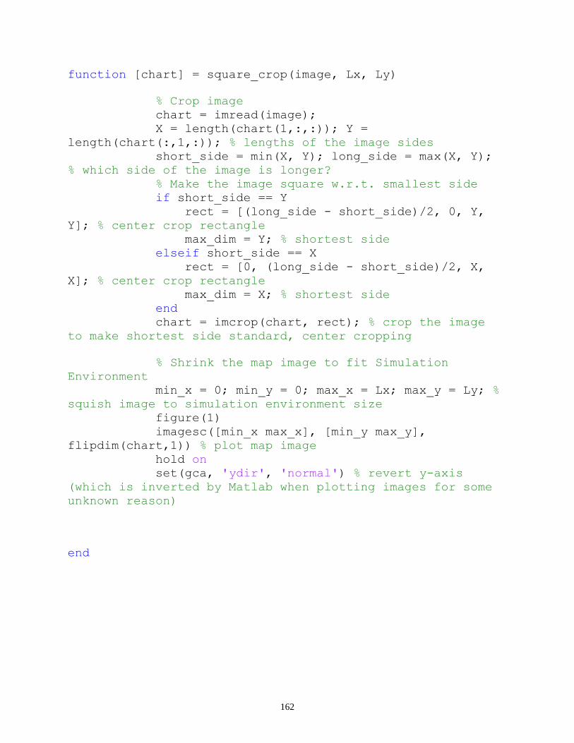
162
function [chart] = square_crop(image, Lx, Ly)
% Crop image
chart = imread(image);
X = length(chart(1,:,:)); Y =
length(chart(:,1,:)); % lengths of the image sides
short_side = min(X, Y); long_side = max(X, Y);
% which side of the image is longer?
% Make the image square w.r.t. smallest side
if short_side == Y
rect = [(long_side - short_side)/2, 0, Y,
Y]; % center crop rectangle
max_dim = Y; % shortest side
elseif short_side == X
rect = [0, (long_side - short_side)/2, X,
X]; % center crop rectangle
max_dim = X; % shortest side
end
chart = imcrop(chart, rect); % crop the image
to make shortest side standard, center cropping
% Shrink the map image to fit Simulation
Environment
min_x = 0; min_y = 0; max_x = Lx; max_y = Ly; %
squish image to simulation environment size
figure(1)
imagesc([min_x max_x], [min_y max_y],
flipdim(chart,1)) % plot map image
hold on
set(gca, 'ydir', 'normal') % revert y-axis
(which is inverted by Matlab when plotting images for some
unknown reason)
end

163
function [Va, beta] = starboard(Vt, twa, Vs)
% Apparent Wind Speed and Apparent Wind Angle
Va = sqrt(Vt^2 + Vs^2 - 2*Vt*Vs*cosd(180-twa)); %
[m/s] apparent windspeed
beta = acosd((Vs + Vt*cosd(twa))/Va); % [degrees]
apparent wind angle relative to the desired course of sail
end
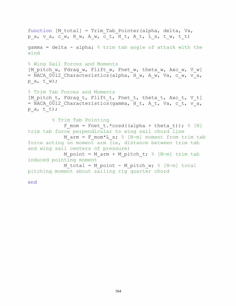
164
function [M_total] = Trim_Tab_Pointer(alpha, delta, Va,
p_a, v_a, c_w, H_w, A_w, c_t, H_t, A_t, L_s, t_w, t_t)
gamma = delta - alpha; % trim tab angle of attack with the
wind
% Wing Sail Forces and Moments
[M_pitch_w, Fdrag_w, Flift_w, Fnet_w, theta_w, Axc_w, V_w]
= NACA_0012_Characteristics(alpha, H_w, A_w, Va, c_w, v_a,
p_a, t_w);
% Trim Tab Forces and Moments
[M_pitch_t, Fdrag_t, Flift_t, Fnet_t, theta_t, Axc_t, V_t]
= NACA_0012_Characteristics(gamma, H_t, A_t, Va, c_t, v_a,
p_a, t_t);
% Trim Tab Pointing
F_mom = Fnet_t.*cosd((alpha + theta_t)); % [N]
trim tab force perpendicular to wing sail chord line
M_arm = F_mom*L_s; % [N-m] moment from trim tab
force acting on moment arm (ie, distance between trim tab
and wing sail centers of pressure)
M_point = M_arm + M_pitch_t; % [N-m] trim tab
induced pointing moment
M_total = M_point - M_pitch_w; % [N-m] total
pitching moment about sailing rig quarter chord
end

165
function [x_dest, y_dest] = upwind_downwind(x_dest, y_dest,
dl, wind, scw)
NoGo_up = 20; % [deg] size of no-go window when sailing
upwind
NoGo_down = 10; % [deg] size of no-go window when sailing
downwind
SF_up = 20; % [deg] upwind safety factor: angle beyond no-
go to be sailed
SF_down = 20; % [deg] downwind safety factor: angle beyond
no-go to be sailed
DesPos = [x_dest, y_dest]*dl; % [m] desired positions of
boat, in meters instead of relative grid spacing
% Check for upwind and downwind sections
x_dest_length = 0;
while length(x_dest) ~= x_dest_length
x_dest_length = length(x_dest);
for j = 2:length(x_dest)
DirCor = mod(atand((DesPos(j,1)-DesPos(j-
1,1))/(DesPos(j,2)-DesPos(j-1,2))), 180) + 180*(0.5 -
0.5*abs((DesPos(j,1)-DesPos(j-1,1)))/(DesPos(j,1)-DesPos(j-
1,1))); % [deg] direct desired course of sail
WinAng = mod(atand(wind(round(DesPos(j-1,2)/dl),
round(DesPos(j-1,1)/dl),1)/wind(round(DesPos(j-1,2)/dl),
round(DesPos(j-1,1)/dl),2)), 360); % Wind angle at current
positon relative to North
Dist = sqrt((DesPos(j,1)-DesPos(j-1,1))^2 +
(DesPos(j,2)-DesPos(j-1,2))^2); % [m] direct distance to
destination
twa = mod((WinAng - DirCor), 360); % true wind angle
relative to boat heading
% Upwind
if (360-NoGo_up)<twa || twa<(NoGo_up)
disp('upwind')
twa_up = twa;
if twa_up>(360-NoGo_up)
twa_up = 360-twa_up; % [deg] reduce true wind
angle to positive angles
end
x_hold = x_dest; y_hold = y_dest; % dummy variables
to hold the route coordinates
166
opt_ang_0 = NoGo_up - twa_up + SF_up; % [deg]
port deviation from course when upwind conditions occur
opt_ang_360 = NoGo_up + twa_up + SF_up; % [deg]
starboard deviation from course when upwind conditions
occur
dist_0 = 0.5*scw/tand(opt_ang_0); % [km] distance
progressed towards destination with every port tack
dist_360 = 0.5*scw/tand(opt_ang_360); % [km]
distance progressed towards destination with every
starboard tack
tacks = ceil(Dist/((dist_0 + dist_360)/2)); %
round down to integer to avoid overshoot
tacks = tacks + 1 - factorial(1-(-1)^tacks); %
ensure an even number of tacks in order to end upwind
manuevers on desired line
sf = 2*Dist/(tacks*(dist_0+dist_360)); % scale
factor to ensure acheiving target point
opt_ang_0 = atand(0.5*scw/(sf*dist_0)); % [deg]
port deviation angle modified to acheive target point
opt_ang_360 = atand(0.5*scw/(sf*dist_360)); %
[deg] starboard deviation angle modified to acheive target
point
h_1 = 0.5*scw/sind(opt_ang_0); % [m] sailing
distance travelled over port tack
h_2 = 0.5*scw/sind(opt_ang_360); % [m] sailing
distance travelled over starboard tack
sig_1 = opt_ang_0 - DirCor; % [deg] angle of
first tack with respect to north
sig_2 = opt_ang_360 + DirCor - 90; % [deg]
angle of second tack w.r.t. north
% Zig-Zag Loop
xx = 0;
for k = j:j+tacks-1
if factorial(1-(-1)^k) < 1.5 && xx^2 < 0.5
% disp('1')
xx = xx-0.5;
x_dest(k) = x_dest(k-1)-h_1*sind(sig_1);
y_dest(k) = y_dest(k-1)+h_1*cosd(sig_1);
elseif factorial(1-(-1)^k) > 1.5 && xx^2 <
0.5
% disp('2')
xx = xx-0.5;
x_dest(k) = x_dest(k-1)+h_2*cosd(sig_2);

167
y_dest(k) = y_dest(k-1)-h_2*sind(sig_2);
elseif factorial(1-(-1)^k) < 1.5
% disp('3')
xx = abs(xx)-xx;
x_dest(k) = x_dest(k-1)+h_2*cosd(sig_2);
y_dest(k) = y_dest(k-1)-h_2*sind(sig_2);
elseif factorial(1-(-1)^k) > 1.5
% disp('4')
xx = abs(xx)-xx;
x_dest(k) = x_dest(k-1)-h_1*sind(sig_1);
y_dest(k) = y_dest(k-1)+h_1*cosd(sig_1);
end
end
% Repopulate the course incorporating the upwind
zig-zag procedure
for i = 1:length(x_hold)-j
x_dest(j+tacks+i-1) = x_hold(j+i);
y_dest(j+tacks+i-1) = y_hold(j+i);
end
DesPos = [x_dest, y_dest]*dl;
% Downwind
elseif (180-NoGo_down)<twa && twa<(180+NoGo_down)
disp('downwind')
twa_down = abs(twa-180);
x_hold = x_dest; y_hold = y_dest; % dummy variables
to hold the route coordinates
opt_ang_0 = NoGo_down - twa_down + SF_down; %
[deg] port deviation from course when downwind conditions
occur
opt_ang_360 = NoGo_down + twa_down + SF_down; %
[deg] starboard deviation from course when downwind
conditions occur
dist_0 = abs(0.5*scw/tand(opt_ang_0)); % [km]
distance progressed towards destination with every port
tack
dist_360 = abs(0.5*scw/tand(opt_ang_360)); % [km]
distance progressed towards destination with every
starboard tack
tacks = ceil(Dist/((dist_0 + dist_360)/2)) %
round down to integer to avoid overshoot

168
tacks = tacks + 1 - factorial(1-(-1)^tacks); %
ensure an even number of tacks in order to end upwind
manuevers on desired line
sf = 2*Dist/(tacks*(dist_0+dist_360)); % scale
factor to ensure acheiving target point
opt_ang_0 = atand(0.5*scw/(sf*dist_0)); % [deg]
port deviation angle modified to acheive target point
opt_ang_360 = atand(0.5*scw/(sf*dist_360)); %
[deg] starboard deviation angle modified to acheive target
point
h_1 = 0.5*scw/sind(opt_ang_0); % [m] sailing
distance travelled over port tack
h_2 = 0.5*scw/sind(opt_ang_360); % [m] sailing
distance travelled over starboard tack
sig_1 = opt_ang_0 - DirCor; % [deg] angle of
first tack with respect to north
sig_2 = opt_ang_360 + DirCor - 90; % [deg]
angle of second tack w.r.t. north
% Zig-Zag Loop
xx = 0;
for k = j:j+tacks-1
if factorial(1-(-1)^k) < 1.5 && xx^2 < 0.5
% disp('1')
xx = xx-0.5;
x_dest(k) = x_dest(k-1)-h_1*sind(sig_1);
y_dest(k) = y_dest(k-1)+h_1*cosd(sig_1);
elseif factorial(1-(-1)^k) > 1.5 && xx^2 <
0.5
% disp('2')
xx = xx-0.5;
x_dest(k) = x_dest(k-1)+h_2*cosd(sig_2);
y_dest(k) = y_dest(k-1)-h_2*sind(sig_2);
elseif factorial(1-(-1)^k) < 1.5
% disp('3')
xx = abs(xx)-xx;
x_dest(k) = x_dest(k-1)+h_2*cosd(sig_2);
y_dest(k) = y_dest(k-1)-h_2*sind(sig_2);
elseif factorial(1-(-1)^k) > 1.5
% disp('4')
xx = abs(xx)-xx;
x_dest(k) = x_dest(k-1)-h_1*sind(sig_1);
y_dest(k) = y_dest(k-1)+h_1*cosd(sig_1);
end
169
end
% Repopulate the course incorporating the upwind
zig-zag procedure
for i = 1:length(x_hold)-j
x_dest(j+tacks+i-1) = x_hold(j+i);
y_dest(j+tacks+i-1) = y_hold(j+i);
end
DesPos = [x_dest, y_dest]*dl;
end
end
end
end

170
function wind = wind_field(Lx,Ly,dl,Vt,Wd)
% Discritize the Environment Space
Lx_steps = Lx/dl; % number of grid steps in x-
direction
Ly_steps = Ly/dl; % number of grid steps in y-
direction
% Initialize wind vector field
wind = zeros(Ly_steps, Lx_steps, 2);
% wind = zeros(Ly, Lx, 2);
% Populate wind vector field
for i = 1:Ly_steps
for j = 1:Lx_steps
wind(i,j,:) = [-Vt*sind(Wd), -
Vt*cosd(Wd)];
end
end
end