field strength and power estimator - rohde & schwarz the field strength from transmitted power...

Subject to change – A. Winter, L.Yordanov 06.2005 – 1MA85_1E

Rohde&Schwarz Products: Various Antennas, Receivers, Spectrum Analyzers and Field Strength Measurement Equipment

Field Strength and Power Estimator

Application Note 1MA85 Determining the field strength from transmitted power is not an easy job. Various, quite complicated formulas have to be evaluated correctly. This application note explains how to calculate electric and magnetic field strength, and power flux density.

A program associated with this application note helps with the calculation and converts Watts to mW and dBm, V/m to V/m and dBV/m as well as A/m to A/m and dBA/m. Additional applications are calculation of propagation loss or antenna factor e.g.

Power Flux Density

1MA85_1E 2 Rohde & Schwarz

Contents 1 Introduction.............................................................................................. 2 2 Software Features And Formulas ........................................................... 2

Power Flux Density ............................................................................ 3 Antenna Characteristics ..................................................................... 4 Receiving Signals and Measuring Power Flux Density...................... 5 Receiving Signals and Measuring Electric Field Strength.................. 5 Receiving Signals and Measuring Magnetic Field Strength............... 6

3 Installing and Starting Field Strength and Power Estimator .................... 7 4 Operating the Program............................................................................ 9

Entering numerical values:............................................................... 10 Starting Calculation .......................................................................... 11 Save and Recall Settings ................................................................. 11 Help and About Menu ...................................................................... 11

5 Some Examples .................................................................................... 13 Determining the Propagation Attenuation between 2 Antennas ...... 13 Determining the Transmit Power for a GPS Simulation................... 14 Using EIRP....................................................................................... 14 Calculating Antenna Factor from Antenna Gain .............................. 15

6 Hardware and Software Requirements ................................................. 16 Hardware Requirements .................................................................. 16 Software Requirements ................................................................... 16

7 Additional Information ........................................................................... 16 8 Ordering Information ............................................................................. 16

1 Introduction Determining the field strength from transmitted power and frequency is not an easy job. This application note explains how to calculate electric and magnetic field strength, and power flux density.

The program Fieldstrength and Power Estimator available with this applica-tion note helps with the calculation and converts mW to dBm, V/m to V/m and dBV/m as well as A/m to A/m and dBA/m.

An introduction of the program features and the calculation formulas is presented.

Information about installing and operating the program are given.

Some examples show additional applications of the program.

2 Software Features And Formulas The program Fieldstrength and Power Estimator calculates power flux density, electric and magnetic field strength from the transmitted power, associated frequency and gain of the transmitting antenna.

Additionally the input power into a receiver with 50 Ohm input impedance is calculated from the gain of the receiving antenna.

The program automatically converts power flux density into electric and magnetic field strength.

Depending on the transmitted frequency, various parameters influence the received power and field strength, such as Non-line-of-sight propagation,

Power Flux Density


changes in polarisation, reflections, and multi path propagation affect the true values. Additionally antenna VSWR and cable losses have to be considered.

The program Fieldstrength and Power Estimator does not consider these impairments. It assumes conditions, that are close to the best possible theoretical values. This is why we say the program is an Estimator, not a Calculator.

Power Flux Density The power flux density and the resulting electric and magnetic fieldstrength are calculated from following formulas:

2t

R4PS**

A transmitter of power Pt (measured in Watts W) feeds an isotropical an-tenna (see Antenna Characteristics below for an explanation of isotropical). This causes a power flux density S (in Watts per square meters W/m2) in the distance R (in meters m) to the transmitter. The magnitude of the power flux density S is simply calculated by dividing the transmitted power Pt by the surface of a sphere with a radius of R meters.

If the transmitter antenna has some gain Gt over an isotropical antenna, the transmited power is concentrated to a part of the sphere´s surface. The power flux density is then:

2tt

R4PGS

**

*

The power flux density is the product of electric and magnetic field strength:

HES *

At a sufficiently large distance from the transmitting antenna, electric and magnetic field strength are proportional to each other. “Sufficiently large” means more than 4(being the wavelength of the transmitted signal in meters). Distances from to 4 give good results, though under certain circumstances the values may not be too precise.

0ZHE

Similar to the relation voltage divided by current, which is the resistance, electric field strength divided by magnetic field strength is a resistance Z0. Z0 is the characteristic impedance of free space.

Ohms377*ð1200Z0

0

With this E resp. H are derived from S as follows:

0ZSE *

0ZSH

Antenna Characteristics


E is measured in V/m (Volts per meter), µV/m (microvolts per meter) or dBµV/m (decibels over 1 microvolt per meter).

H is measured in A/m (amperes per meter), µA/m (microamperes per me-ter) or dBµA/m (decibels over 1 microampere per meter).

Antenna Characteristics An antenna picks up some energy from the power flux density. As real an-tennas always have some size, we can define the effective electric area of an antenna in terms of an area, which picks up some power from the power flux density.

The effective area of an isotropical antenna is given as

22i 08041A

*.**

Ai is measured in m2 (square meters).

An isotropical antenna theoretically radiates equally in each direction. In practice, isotropical antennas do not exist. Real existing antennas always concentrate the radiated energy into some preferred directions. The characteristics of transmitting antennas and receiving antennas are the same. Thus the effective area of these antennas always is somewhat greater than the effective area of isotropical antennas (assumed that there are no losses). We say, a real antenna with an effective area A has some gain G over an isotropical antenna:

*

**4

GAGA2

i

The effective area of a commonly used dipole is:

2D 130A *. so

ii

DD dB126251

080130

AAG ..

.

.

The gain GD of a dipole is 1.625 or 2.1 dBi, as 10*log10(1,625) equals 2.1 dB.

The power Pr which we can get from a certain power flux density S by using an antenna of an effective area Ar is:

rr ASP *

As S is measured in W/m2 and Ar in m2, we get the power Pr in W (Watts).

It is more common however, to express the power in mW (milli Watts, milli means one thousends of a Watt) or in a logarithmical scale, then we get dBm.

Logarithmical scales always represent a ratio of 2 values. So dBm means the power referred to 1 mW (1 milli Watt = 1 thousandth of a Watt) ex-pressed in dB (deciBel). Bel is the logarithm to the base 10, decibel is the tenth of a Bel, we have to multiply Bel values by 10 to get deciBel):

mWmWPdBmP r

r /1

/log*10/ 10

Receiving Signals and Measuring Power Flux Density


Please read this formula as follows:

Pr in dBm is 10 times the logarithm of Pr in mW divided by 1 mW.

Receiving Signals and Measuring Power Flux Density In order to measure the power flux density, we need a receiver or a spec-trum analyser and an antenna. As explained above, the receiving antenna picks up the power Pr from the electromagnetic field with it´s effective antenna area Ar. If we feed this power into the input of the receiver or spectrum analyzer, we can measure it. As we certainly know the effective electric area or the gain of our antenna, we can measure the power flux density S of the electromagnetic field as follows:

With rr ASP * we get

r

r

APS

Remembering that the effective area Ar of an antenna is:

*

**4

GAGA2

rirr

where Gr means the gain of the receiving antenna over an isotropic antenna of area Ai or /4

Example: We want to measure the power flux density of a GSM base station transmitter at 900 MHz with a spectrum analyzer and a dipole antenna. 900 MHz corresponds to a wavelength of 0.332 m. The spectrum analyzer shows a power of 2 mW or 3 dBm. An isotropic antenna has an area of 0.08*, this is 0.08*0.332 m*0.332 m =0.0088 m2. A dipole antenna has a gain of 1.625, so it´s area is 0.0143m2. With this, the power flux density is 139.6 mW/m2 or 21.5 dBm/m2.

Receiving Signals and Measuring Electric Field Strength We can also determine the electric field strength in a similar way. With:

0ZSE *

we get:

0r

r ZAPE *

If our receiver shows the input voltage Ur at an input impedance of Zi (nor-mally 50 Ohm), then we have to use the following relationship between in-put power Pr and input voltage Ur.

i

2r

r ZUP

Using this we get:

Receiving Signals and Measuring Magnetic Field Strength


0ri

2r Z

A1

ZUE ** or, by rearranging the formula:

i

o

rr Z

ZA1UE **

The square root expression is also known as antenna factor Ka:

i

02

ri

0

ra Z

ZG4

ZZ

A1K *

*

**

Gr is the receiver antenna gain over an isotropic antenna, is the wave-length of the received signal, Z0 is the propagation impedance of free space (377 ) and Zi the receiver input impedance (normally 50 ), so:

ar KUE *

Sometimes Ka is expressed in dB:

)(log*20/ 10 aa KdBK

Electric field strength is measured in V/m or in V/m. In order to convert to V/m, remember that 1V = 1000000 V (1million micro Volts).

Example: 0.0003 V/m = 300 V/m

You can also convert the field strength from V/m to dBV/m using follow-ing equation:

V/m/1V/m/

log*20V/m/ 10 EdBE

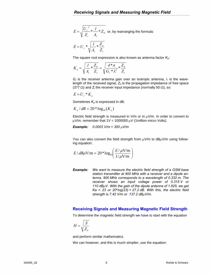
Example: We want to measure the electric field strength of a GSM base station transmitter at 900 MHz with a receiver and a dipole an-tenna. 900 MHz corresponds to a wavelength of 0.332 m. The receiver shows an input voltage power of 0.315 V or 110 dBV.. With the gain of the dipole antenna of 1.625, we get Ka = 23 or 20*log(23) = 27.2 dB. With this, the electric field strength is 7.42 V/m or 137.2 dBV/m.

Receiving Signals and Measuring Magnetic Field Strength To determine the magnetic field strength we have to start with the equation

0ZSH

and perform similar mathematics.

We can however, and this is much simplier, use the equation:



0ZEH

and determine the electric fieldstrength first (remember Z0 = 377 . Then we simply have to divide this value by 377 .

Magnetic field strength is measured in A/m or in A/m. In order to convert to A/m, remember that 1 A = 1000000 A (1 million micro Amperes).

Example: 0.0003 A/m = 300 A/m.

You can also convert the field strength from A/m to dBA/m using follow-ing equation

/m/1/m/

log*20/m/ 10 AAHAdBH

Example: We want to measure the magnetic field strength of a GSM base station transmitter at 900 MHz with a receiver and a dipole antenna. 900 MHz corresponds to a wavelength of 0.332 m. The receiver shows an input voltage power of 0.315 V or 110 dBV..Determine the electric field strength first as above. With the gain of the dipole antenna of 1.625, we get Ka = 23 or 20*log(23) = 27.2 dB. With this, the electric field strength is 7.42 V/m. In order to get the magnetic field strength, we divide this value by 377 and get 0.0197 A/m or 85.9 dBA/m.

3 Installing and Starting Field Strength and Power Estimator To install the Fieldstrength and Power Estimator program execute the file FieldStrengthEstimator_<version number>.exe with a double click. The in-stallation wizard is activated; the first option is choose the language (Eng-lish or German) for the installation.

Follow the instructions from the wizard. In the course of the installation se-lect the directory of your choice in which the program is to be installed.

Fieldstrength and Power Estimator requires approximately 1 MB RAM on a hard disk. The wizard also adds an entry for Fieldstrength and Power Estimator in the Start->Programs menu of the computer.

No other parameters are required for installation.

For de-installation, Rohde & Schwarz supplies the program uninstall.exe, which removes the program Fieldstrength and Power Estimator completely from the computer.

Warning: De-install removes the program files and also the directory in which Fieldstrength and Power Estimator in installed. Make sure you have archived any other files or subdirectories pre-sent in the directory before de-installation.



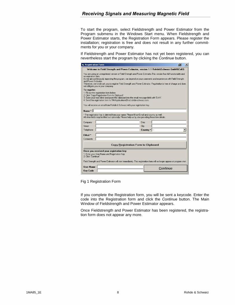
To start the program, select Fieldstrength and Power Estimator from the Program submenu in the Windows Start menu. When Fieldstrength and Power Estimator starts, the Registration Form appears. Please register the installation; registration is free and does not result in any further commit-ments for you or your company.

If Fieldstrength and Power Estimator has not yet been registered, you can nevertheless start the program by clicking the Continue button.

Fig 1 Registration Form

If you complete the Registration form, you will be sent a keycode. Enter the code into the Registration form and click the Continue button. The Main Window of Fieldstrength and Power Estimator appears.

Once Fieldstrength and Power Estimator has been registered, the registra-tion form does not appear any more.



Fig 2 Fieldstrength and Power Estimator Main Window

Click the Formulas button to show the calculation formulas.

4 Operating the Program To enter values for your calculation, select the appropriate field either with a left click of your mouse, by using the TAB key (forward order) or pressing Shift and TAB key simultaneously (reverse order).

Since some values depend on previously entered values, you should use the following order:

1. Frequency

2. Gain of transmitting antenna

3. Gain of receiving antenna

4. Distance of transmitter to receiver

5. Transmitted power

Enter a value and confirm your entry by pressing the ENTER key. If you just want to change only one digit of an existing entry, select this digit with your mouse or with the <> cursor keys.

If you want to use a different unit for your entry, select the new unit first. You can use the TAB /ShiftTAB keys to select the unit field. Use UP and DOWN

keys to select the new unit or use the selection function with your mouse.

Fig 3 Selecting Units

Entering numerical values:


Depending on the language settings of your computer´s operation system, a colon or a dot is used as a decimal separator.

Entering numerical values: The following inputs all result in the same value:

123.45E-7

12.345µ, you can use also u for = micro

0.000012345

Note, that entries are made using the selected units. For example: 0.001 with unit mW results in a value of 1 Microwatt.

If basic units like Hz, m, W, V/m or A/m are selected, you can use the SI symbolic abbreviations for the exponent of your number. Example: 123M (M for Mega) together with Hz gives 123000000 Hz. Values of 0 and negative values are only allowed if the unit is in dB, otherwise an error message will occur.

in SI SI Factor words prefix symbol

1.0E+21 sextillion zetta Z 1.0E+18 quintillion exa E 1.0E+15 quadrillion peta P 1.0E+12 trillion tera T 1.0E+9 billion giga G 1.0E+6 million mega M 1.0E+3 thousand kilo k 1.0E+2 hundred hecto h 1.0E+1 ten deka da 1.0E 0 initial value one - 1.0E-1 tenth deci d 1.0E-2 hundredth centi c 1.0E-3 thousandth milli m 1.0E-6 millionth micro µ 1.0E-9 billionth nano n 1.0E-12 trillionth pico p 1.0E-15 quadrillionth femto f 1.0E-18 quintillionth atto a 1.0E-21 sextillionth zepto z

1.0E-24 septillionth yocto y

Fig 4 Exponential abbreviations

Starting Calculation


Starting Calculation To start calculation, press the ENTER key. The value is calculated to 15 significant figures, the results however are displayed with a 3 decimal places only.

If you change a units field, the corresponding numerical values are con-verted. For example: 1 mW gives 0 dBm if the unit is changed from mW to dBm. Be careful not to change a zero linear value to dB.

The calculation is also done when you leave an entry field with the TAB key. In this case, the program will use the displayed values. Going forth and back through the entry fields with the TAB / Shift TAB keys will result in a small change of all values due to the 3 decimal places only shown on the display.

When changing the values for Frequency, Antenna Gain Transmitter, An-tenna Gain Receiver or Distance, all other values are recalculated using the set Transmitted Power.

When changing one of the other values however, Frequency, Antenna Gain Transmitter, Antenna Gain Receiver and Distance will keep their values.

If you enter a Distance value, which is smaller than 0.159 times the wave-length (</2), the distance entry field becomes yellow as a warning for leaving the far-field condition.

Fig 5 Near-Field Warning

Save and Recall Settings On exiting the program, all numerical values and units are saved to a file settings.ini in the program directory. Upon restart, these values are auto-matically restored. For convenience of operation, you can Save and Open Settings dialog. Use Default Settings to get a well defined program state.

Fig 6 Save and Recall Settings

Help and About Menu

Help and About Menu


Fig 7 Help Menu

For convenient use of the program and recalling the explanation of the cal-culation formulas, selecting Field Estimator Help will show you this docu-mentation.

On selecting About, the following menu will show up:

Fig 8 About Menu

The button legal information shows the conditions for using this program.

The buttons driver information and system information will display informa-tion on some installed drivers and your operating system. You can use the button copy support information to clipboard for debugging computer prob-lems. Paste your clipboard contents to your mail system and send it to [email protected].

mailto:[email protected]

Determining the Propagation Attenuation between 2 Antennas


5 Some Examples The following examples show some of the additional capabilties of the pro-gram Field Strength and Power Estimator. Please note, that there are cor-responding setting files available in your installation directory. You can load them in the File/Open Settings menu.

Determining the Propagation Attenuation between 2 Antennas You can determine the attenuation of an undistorted wave progagation as follows:

Enter the frequency, set the antenna gains of transmit and receive anten-nas to 0 dBi and enter the distance. If you enter 0 dBm for transmitted power, the field Received Power in dBm will show the value of the attenua-tion in dB.

Example: Satellites of the ASTRA TV system for Europe are geostationary satellites positioned at 19.3° East. They transmit at frequencies around 12 GHz. Geostationary satelites orbit at a height of 35785 km above the equator. The distance from satellite to the city of Munich (the home city of Rohde & Schwarz) is around 38190 km. The program calculates a propa-gation attenuation of 205.67 dB.

Fig 9 Propagation Attenuation at 12 GHz

Determining the Transmit Power for a GPS Simulation


Determining the Transmit Power for a GPS Simulation GPS receivers often have integrated antennas. To test such GPS receivers in your laboratory with a test tranmitter, you have to provide a signal with a field strength similar to real GPS signals transmitted at 1575 MHz. The GPS system makes sure, that a ground receiver gets a power of -165 dBW (= -135 dBm) out of an isotropic antenna. You want to use a dipole antenna 1 m above your GPS receiver. What transmitted power do you have to set at your test transmitter, in order to get the same field strength as from the GPS system?

Set Frequency to 1.575 GHz, transmit antenna gain to 2.1 dBi and distance to 1 m. Now enter a received power of -135 dBm. Pressing the ENTER key will calculate the necessary transmit power as -107.706 dBm. By the way, propagation loss for GPS signals is about -182 dB, since the satellites orbit at a height of 20000 km above earth.

Fig 10 GPS Simulation

Using EIRP Sometimes transmitter power and transmitter antenna gain are not speci-fied separately but as EIRP (Effective Isotropic Radiated Power). EIRP is the product of transmitted power and transmitter antenna gain when using linear values or the sum of both values in dB or dBm. If EIRP is given, use 0 dBi for Antenna Gain Transmitter and enter the EIRP in dBm, mW or W in the field for Transmitter Power.

Calculating Antenna Factor from Antenna Gain


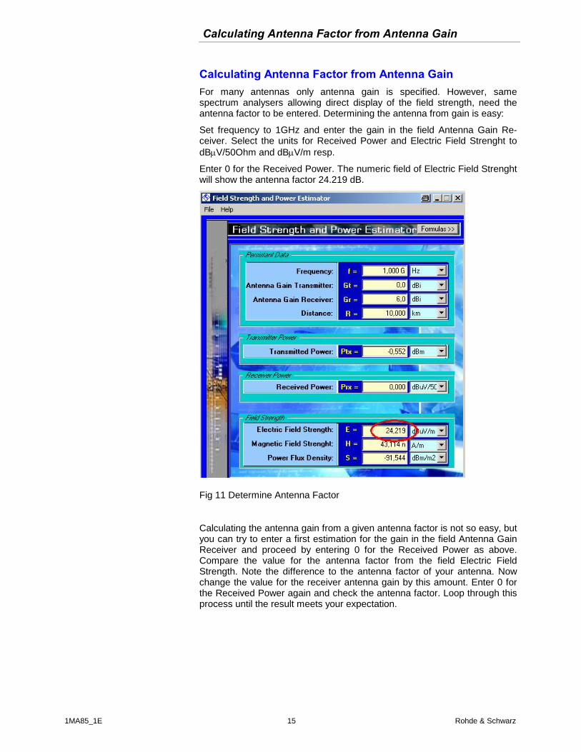
Calculating Antenna Factor from Antenna Gain For many antennas only antenna gain is specified. However, same spectrum analysers allowing direct display of the field strength, need the antenna factor to be entered. Determining the antenna from gain is easy:

Set frequency to 1GHz and enter the gain in the field Antenna Gain Re-ceiver. Select the units for Received Power and Electric Field Strenght to dBV/50Ohm and dBV/m resp.

Enter 0 for the Received Power. The numeric field of Electric Field Strenght will show the antenna factor 24.219 dB.

Fig 11 Determine Antenna Factor

Calculating the antenna gain from a given antenna factor is not so easy, but you can try to enter a first estimation for the gain in the field Antenna Gain Receiver and proceed by entering 0 for the Received Power as above. Compare the value for the antenna factor from the field Electric Field Strength. Note the difference to the antenna factor of your antenna. Now change the value for the receiver antenna gain by this amount. Enter 0 for the Received Power again and check the antenna factor. Loop through this process until the result meets your expectation.

Hardware Requirements


6 Hardware and Software Requirements

Hardware Requirements CPU: Pentium 300 MHz or better

Hard Disk: 1 MByte free

Monitor: SVGA color monitor, resolution 800x600 or better

Software Requirements The program was tested with Microsoft 32-bit operating systems (Windows 95/98/NT/2000/ME/XP)

7 Additional Information This application note and the associated program Fieldstrength and Power Estimator are updated from time to time. Please visit the website 1MA85 in order to download new versions. After installation, the latest program infor-mation can be found in the file history.rtf in the installation directory. You can access this file also from link Programs / Field Strength Estimator / History from your Start Programs folder.

Please send any comments or suggestions about this application note to [email protected].

8 Ordering Information Please note, that complete solutions for field strength and power measure-ments for various applications are available from Rohde & Schwarz.

For additional information about antennas, receivers, spectrum analysers and fieldstrength measurement equipment, see the Rohde & Schwarz website www.rohde-schwarz.com.

ROHDE & SCHWARZ GmbH & Co. KG . Mühldorfstraße 15 . D-81671 München . Postfach 80 14 69 . D-81614 München .

Tel (089) 4129 -0 . Fax (089) 4129 - 13777 . Internet: http://www.rohde-schwarz.com

This application note and the supplied programs may only be used subject to the conditions of use set forth in the download area of the Rohde & Schwarz website.

http://www.rohde-schwarz.com/appnote/1ma85.html

mailto:[email protected]

www.rohde-schwarz.com

http://www.rohde-schwarz.com/

field strength and power estimator - rohde & schwarz the field strength from transmitted power...

Documents