Final PresentationFourth Order Very Fast Voltage

Regulator for RF PA

Performed by: Tomer Ben Oz Yuval Bar-Even

Guided by: Shahar Porat

Background• Mobile devices such as smartphones, tablet and laptop required to support

wireless communication, and yet, to be able to run for a long period of time with out charging.

• One of the most energy consumer in wireless module is the Power Amplifier (PA) that connected to the RF antenna.

• Recent trend to reduce the total power of the PA, is by applying Envelope tracking (ET) on the PA supply level. By using this technique, the power of the PA will be change as a results of the required power for transmitting.

• In order to apply high efficiency ET, there is a need to use Switching Voltage Regulator (SVR), and not Linear Voltage Regulator (LVR).

• In order to reduce frequency switching noise on the PA supply, a 4th order SVR is being proposed.

Project target

• Develop a 4th order, high bandwidth Switching Voltage Regulator (SVR), that will be able to supply RF PA, as describe in the figure below.

Project objectives

• Design and stabilize a high efficiency, high BW fourth order voltage regulator.

• Build a good understanding on how each component affects the stability and accuracy for the “real world” implementation of the voltage regulator.

Design Requirements• Very low power consumption.

• Ripples and overshoot of below 5%.

• SSE of at least 2%.

• Phase margin of at least 35.

• 1 [MHz] envelope tracking bandwidth.

The phases of the project

1. Simple closed loop design

2. Buck converter

3. Adding a compensator

4. Fourth order system

5. Adding Equivalent Series Resistance

Working environment

• Simulink via Matlab

• Cadence’s virtuoso.

Simple closed loop design

• Understanding The Principle

1lim

out in

out inA

AV V

AV V

𝐴

Simple closed loop design

• Advantages:• High Bandwidth• Low Overshoot• Simple to design

• Disadvantage:• Power Consumption

Buck converter - Transient

max min

(1 )

(1 )

i O O Diode

O i Diode

II I T DutyCycle

T

V V V VT DutyCycle T DutyCycle

L L

V V DutyCycle V DutyCycle

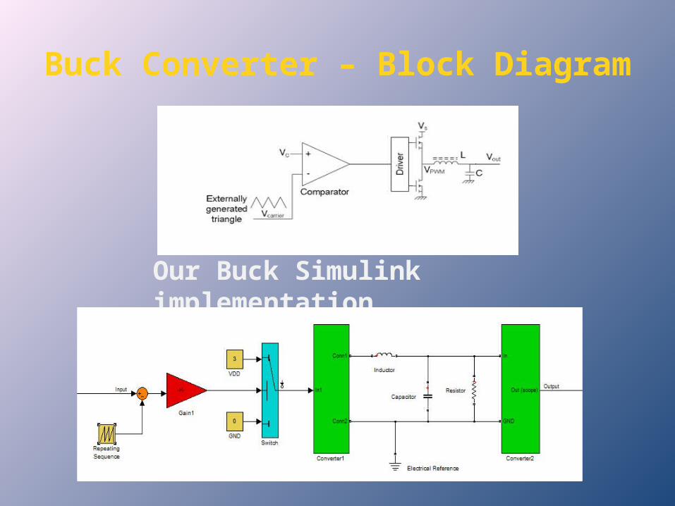
Buck Converter – Block Diagram

Our Buck Simulink implementation

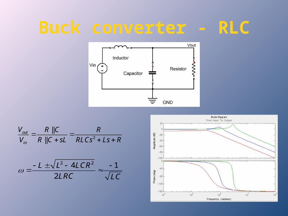
Buck converter - RLC

2

||

||out

in

V R C R

V R C sL RLCs Ls R

2 24 1

2

LCRL L

LR LC C

Buck converter - PWM

cV BDutyCycle

A B

cO DD DD

DD DDO c

V BV V DutyCycle V

A B

V V BV V

A B A B

DDO c

VV V

A

A

B

Vc

-Buck converter Frequency domain

Buck converter simulation

Buck output for given sine wave input

10switchingf

LC sin

1f

LC

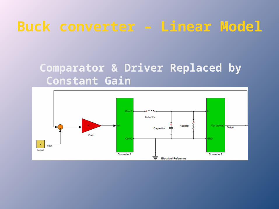
Buck converter – Linear Model

Comparator & Driver Replaced by Constant Gain

Buck converter - Open Loop Bode

On the Cross Over point the phase margin is 8

So What Is A Compensator

1 1 2 2

1 2

(1 ) (1 )Out

In

V s RC s R C

V s RC

1

2 2

2

1 1

0

1

2

1

2

Pole

Zero

Zero

f

fR C

fRC

Compensator – Bode Diagram

Locating the Zeroes give the open loop system 90boost

Considerations of choosing the locations of the Zeros

• The zeros should give a phase boost of at least 35 at the Cross Over.

• There is a need to filter the switching frequency and it requires a large attenuation.

• Increase in the difference of the zeros can move the Cross Over point 0dB.

Adding The Compensator

Adding The Compensator

On the Cross Over point the phase margin is 5

Various Components Values

Degrees of freedom in choosing the component values

Poles Location

Fourth order system

5 5

,1

5 5

,2

4 4

1

1

1

Zeros

Poles

Poles

L C

L C

L C

Canceling each other

Dominant in the TF

Fourth order system – Bode Diagram

After adding the 4th order the system is not stable – Negative phase marginCaused by adding more cross over points

Adding Equivalent Series Resistance

The ESR of the inductors add complexity to the Transfer Function but due to their low values one can consider only the damping they apply

ESR Damping Effect

As the ESR increases the damping decreases

Final Components Values

Value Name

10[MOhm] R1

0.159[pF] C1

0.1[MOhm] R2

5.59[pF] C2

300[m Ohm] RL

10[nH] L4

25.4[nF] C4

1[uH] L5

2.56 [uF] C5

Final System – Step Response

Settling time < 1[uS] OverShoot < 2%

Working Frequency – 1[MHz]Phase Margin - 53

Preparing for Part B• Achieving a good understanding of the affects

of each component to the system for:– Stability– Settling time– Sensitivity

Questions?