final project report load modeling …uc-ciee.org/downloads/lm_final_report_appendixg.pdffinal...
TRANSCRIPT

FINAL PROJECT REPORT
LOAD MODELING TRANSMISSION RESEARCH
APPENDIX G WECC LOAD COMPOSITION DATA TOOL SPECIFICATION
Prepared for CIEE By:
Lawrence Berkeley National Laboratory
A CIEE Report


iii
Table of Contents
Abstract ..................................................................................................................................................... vii
1.0 Nomenclature ................................................................................................................................ 1
2.0 Introduction ................................................................................................................................... 3
3.0 Use Cases ........................................................................................................................................ 5
3.1. Use Case 1: Feeder Load Composition ......................................................................... 5
3.2. Use Case 2: Substation Load Composition ................................................................... 5
3.3. Use Case 3: Calibrated Load Composition ................................................................... 6
4.0 Requirements ................................................................................................................................. 7
4.1. Location ............................................................................................................................. 8
4.2. Study Information ............................................................................................................ 9
4.3. Climate Data ..................................................................................................................... 9
4.4. Building Design Conditions ......................................................................................... 11
4.5. Substation/Feeder Composition ................................................................................... 12
4.6. Residential Model .......................................................................................................... 13
4.6.1. Single‐Family Dwellings .................................................................................. 13
4.6.2. Multi‐Family Dwellings ................................................................................... 27
4.7. Commercial Model ........................................................................................................ 28
4.7.1. Floor Area .......................................................................................................... 29
4.7.2. Load Shapes ....................................................................................................... 29
4.7.3. Rules of Association ......................................................................................... 30
4.8. Industrial ......................................................................................................................... 31
4.9. Agricultural ..................................................................................................................... 31
4.10. Load Composition ......................................................................................................... 31
4.10.1. Feeder Composition ......................................................................................... 32
4.11. Loadshapes ..................................................................................................................... 32
4.12. Sensitivities ..................................................................................................................... 33
4.13. System‐Wide Results ..................................................................................................... 34
5.0 Prototype ...................................................................................................................................... 37
5.1. Conditions ....................................................................................................................... 37
5.2. Composition ................................................................................................................... 38
5.3. Feeders ............................................................................................................................. 39
5.4. Loadshapes ..................................................................................................................... 39

iv
5.5. Sensitivity ........................................................................................................................ 40
5.6. Residential ....................................................................................................................... 41
5.7. Commercial ..................................................................................................................... 43
5.8. Industrial ......................................................................................................................... 43
5.9. Agricultural ..................................................................................................................... 44
6.0 References .................................................................................................................................... 45

v
Figures
Figure 1. Typical delayed voltage‐recovery profile on a 230 kV transmission circuit. The fault
occurs at (a) and is cleared at (b) after the voltage has dropped to 79% of the nominal
voltage. The dip causes air‐conditioner motors to stall, during which time their current
draw is significantly higher than normal. This situation lasts through (c) until the motorsʹ
thermal protection interrupts the current and the voltage gradually recovers by (d).
Meanwhile, other voltage controls such as load tap changers and capacitor banks cause the
voltage to overshoot (e) and settle out too low (f). ........................................................................ 4
Figure 2. The WECC composite load model structure includes static loads, electronic loads,
constant‐torque three‐phase motors (A), high inertia speed‐squared load motors (B), low
inertia speed‐squared load motors (C), and constant‐torque single‐phase motors (D). .......... 4
Figure 3. Diversified single‐family air‐conditioning load curves. ................................................... 22
Figure 4. The prototype conditions page. ............................................................................................ 37
Figure 5. The prototype feeder composition page. ............................................................................ 38
Figure 6. The prototype substation composition page. ..................................................................... 38
Figure 7. The prototype feeder composition table page. ................................................................... 39
Figure 8. The prototype loadshapes graphs page. ............................................................................. 39
Figure 9. The prototype sensitivity table page. ................................................................................... 40
Figure 10. The prototype residential single‐family design page. ..................................................... 41
Figure 11. The prototype residential multi‐family design page. ...................................................... 42
Figure 12. The prototype residential design page. ............................................................................. 43
Figure 13. The prototype commercial design page. ........................................................................... 43
Figure 14. The prototype industrial design page. .............................................................................. 43
Figure 15. The prototype agricultural design page. ........................................................................... 44

vi
Tables
Table 1. Building types ............................................................................................................................. 7
Table 2. End‐use electrification by city (fraction of homes having electric end‐use) .................... 18
Table 3. Installed end‐use capacities for single‐family residential dwelling .................................. 20
Table 4. Residential air‐conditioner size weighting factors .............................................................. 21
Table 5. SEER model calibration results .............................................................................................. 21
Table 6. Residential end‐use load shapes ............................................................................................ 23
Table 7. Single‐family residential rules of association ....................................................................... 26
Table 8. Multi‐family residential rules of association ........................................................................ 28
Table 9. Commercial building default floor area ................................................................................ 29
Table 10. Rules of association for commercial buildings (except health facilities) ........................ 30
Table 11. Rules of association for health facilities .............................................................................. 31
Table 12. Customer class load composition scalar ............................................................................. 32
Table 13. Customer type on feeders ..................................................................................................... 32
Table 14. Temperature sensitivities ...................................................................................................... 34

vii
Abstract
This document specifies the methodology used by the Load Composition Data Tool developed
for the Western Electricity Coordinating Council (WECC). A composite load model structure
has been previously specified that describes the two salient features of the new model:
(a) recognition of the electrical distance between the transmission bus and the end‐use loads;
and (b) the diversity in the composition and dynamic characteristics of end‐use loads. The load
model includes data for an equivalent model of the distribution feeder, the load components,
and the fractions of the load components. The methodology adopted by the WECC for
identifying the fractions of the load components is specified in this document.

1
1.0 Nomenclature
A area
CEUS California End Use Survey data
COP coefficient of performance
D duty cycle
E electric energy
EER energy efficiency ratio
F fraction
H hour, height
k load basis
L load
LS load shape
m TMY index, month
M motor
N number
P power
PF power factor
Q heat load, capacity
q load density
R thermal resistance value
RH relative humidity
S solar gain, shading
SEER seasonal energy efficiency ratio
T temperature

2
t time
TMY typical meteorological year
UA thermal conductance
v velocity
V volume
W power
Z impedance
ZIP impedance, current, and power

3
2.0 Introduction
A power system model includes three main elements: the sources of power, the transmission of
power, and the loads. Load representation has long been the least accurate of these
three elements. The stability of the system depends on whether the balance between supply and
demand is maintained. When the system is perturbed by an abrupt change in either supply or
demand, the opportunities for part of the system to ʺfall out of stepʺ increase greatly. Dynamic
models are used to examine whether such a risk exists under various conditions, and these
models require accurate descriptions of the system interconnections, as well as both the
generators and the loads.
Work performed in the early 1990s provided initial guidance regarding load modeling (IEEE
Task Force 1993; 1995). The Western Electricity Coordinating Council (WECC) adopted an
interim dynamic load model of the California‐Oregon Intertie (COI) in early 2002 to address
critical operational issues with the COI and formed the WECC Load Modeling Task Force
(LMTF) to develop a permanent composite load model to be used for planning and operation
studies in the long term (Pereira 2002). The composite load model is nearly complete, and
provides a much more accurate representation of the response of load to voltage and frequency
disturbances by offering a much more accurate description of the load behavior during
transmission faults (Kosterev 2008).
Of greatest importance for WECC in this context is the ability to perform dynamic voltage‐
stability studies, the outcomes of which are strongly influenced by the dynamic behavior of
loads. The interim load model is unable to represent delayed voltage recovery from
transmission faults, such as those observed in Southern California since 1990 and reported by
Florida Power and Light (Williams 1992; Shaffer 1997).

4
Figure 1. Typical delayed voltage-recovery profile on a 230 kV transmission circuit. The fault occurs at (a) and is cleared at (b) after the voltage has dropped to 79% of the nominal voltage. The dip causes air-conditioner motors to stall, during which time their current draw is significantly higher than normal. This situation lasts through (c) until the motors' thermal protection interrupts the current and the voltage gradually recovers by (d). Meanwhile, other voltage controls such as load tap changers and capacitor banks cause the voltage to overshoot (e) and settle out too low (f).
It is generally accepted that delayed voltage recovery is related to stalling of residential single‐
phase air conditioners in areas close to the fault. Simulations of these events show instantaneous
post‐fault voltage recovery, in sharp contrast to the observed behavior shown in Figure 1
(Chinn 2006).
Figure 2. The WECC composite load model structure includes static loads, electronic loads, constant-torque three-phase motors (A), high inertia speed-squared load motors (B), low inertia speed-squared load motors (C), and constant-torque single-phase motors (D).

5
3.0 Use Cases
The following use‐cases shall be considered by software developers.
3.1. Use Case 1: Feeder Load Composition Goal
The user seeks to generate a single feeder load model for use with PSLF that incorporates motor
A‐C, ZIP, and electronic load components based on customer survey data.
Inputs
The user provides the following information
1. City
2. Month
3. Day of week
4. Hour of day
5. Number/type of residential and commercial buildings
Outputs
The total load and the fractions motors A‐C, ZIP, and electronic loads.
3.2. Use Case 2: Substation Load Composition Goal
The user seeks to generate a multi‐feeder load model for use with PSLF that incorporates motor
A‐C, ZIP, and electronic load components based on customer survey data.
Inputs
The user provides the following information
1. City
2. Month
3. Day of week
4. Hour of day
5. Number/type of residential and commercial buildings on each feeder
Outputs
The total load and the fractions motors A‐C, ZIP, and electronic loads.

6
3.3. Use Case 3: Calibrated Load Composition Goal
The user seeks to generate a multi‐feeder load model for use with PSLF that incorporates motor
A‐C, ZIP, and electronic load components based on customer meter data.
Inputs
The user provides the following information
1. City
2. Month
3. Day of week
4. Hour of day
5. Number/type of residential and commercial buildings on each feeder
6. Meter scaling results (actual/predicted)
Outputs
The total load and the fractions motors A‐C, ZIP, and electronic loads.

7
4.0 Requirements
The methodology for estimating the fractions of each load component is based on a ʺbottom‐upʺ
approach. For single‐family and multi‐family residential buildings, the model is based on a
thermal and equipment performance model described in Residential Model (Section 4.6).
Table 1. Building types
Load class Building type Floor area
Residential
Single-family home all
Multi-family dwelling all
Commercial
Small office ≤ 30,000 sf
Large office > 30,000 sf
Retail all
Lodging all
Grocery all
Restaurant all
School all
Health all
For commercial buildings, the California Commercial End Use Survey (CEUS) is used as the
primary source for the load shapes of each commercial building type listed in Table 1. These are
described in Commercial Model (Section 4.7).

8
4.1. Location The location shall be requested from the user and shall be a city chosen from among the
supported cities. The default location shall be Portland OR. The supported cities shall include at
least the following
1. Albuquerque NM
2. Bakersfield CA
3. Barstow CA
4. Boise ID
5. Cheyenne WY
6. Denver CO
7. Eugene OR
8. Eureka CA
9. Fresno CA
10. Helena MT
11. Las Vegas NV
12. Long Beach CA
13. Los Angeles CA
14. Phoenix AZ
15. Portland OR
16. Prince George BC
17. Redmond OR
18. Reno NV
19. Richland WA
20. Sacramento CA
21. Salt Lake City UT
22. San Diego CA
23. San Francisco CA
24. Santa Maria CA
25. Seattle WA
26. Spokane WA
27. Yakima WA

9
4.2. Study Information A study is a scenario or case that a user wishes to examine.
All the information pertaining to a study shall be stored in a study file that can be retrieved
later. The data storage requirements must be verifiably repeatable, i.e., a user shall be able to
send a study file to another user, who shall be able to load the study file and produce an
identical result without any additional data entry.
The study information shall include the data needed to determine when and where the load
composition is being evaluated. The default study shall be a summer‐peak weekday.
The following study information shall be requested from the user:
Study type
The study type shall specify the general time of the condition for which the load composition is
being evaluated. It shall be chosen from among the set of allowed study conditions, including
winter peak, typical, and summer peak. The default study type shall be summer peak.
Month
The month, Mstudy, shall be the month for which the study is being evaluated. If the study type is
winter peak, the default month shall be the month during which the lowest temperature is
observed at the location. If the study type is typical, the default month shall be the month with
the minimum cooling and heating degree days. If the study type is summer peak, the default
month shall be the month during which the highest temperature is observed.
Day of week
The day of week, Dstudy, shall be the day for which the study is being evaluated. If the study is
winter peak, the default day of week shall be Monday. If the study is typical or summer peak, the
default day of week shall be Wednesday. In cases where the week day is specified or used as a
digit, Sunday shall be week day 0, Monday day 1, etc.
Hour of day
The hour of day, Hstudy, shall be the hour for which the study is being evaluated. The hour of day
shall be specified as an integer between 0 and 23. If the study is winter peak, the default hour of
day shall be the early morning hour of the coldest day at which the Monday morning setup
occurs (typically between 5am and 8am). If the study is typical or summer peak, the default hour
of day shall be the afternoon hour at which the peak load is observed (typically between 3pm
and 6pm).
4.3. Climate Data The climate data shall be that which is given by the Typical Meteorological Year version 2 data
for the feeder location. The default climate data shall be for the current study city (NREL
TMY2).

10
The weather data for the study conditions shall based on the climate data at the time of the
study. The following data shall be obtained from the TMY2 data:
Dry‐bulb temperature
The dry‐bulb outdoor air temperature shall be specified in degrees Fahrenheit(°F), and the
default dry‐bulb air temperature shall be TMY drybulb temperature at the cooling design
condition
(1)
Wind speed
The wind speed shall be specified in miles per hour (mph) and the default wind speed shall be
the TMY wind speed at the cooling design condition
(2)
When more than one maximum temperature is found in the TMY temperature data, then the
maximum wind speed for all those observations is to be used.
Relative humidity
The relative humidity shall be specified in percent(%), and the default relative humidity shall be
the TMY relative humidity at the cooling design condition
(3)
When more than one maximum temperature is found in the TMY temperature data, then the
maximum relative humidity for all those observations is to be used.
Opaque sky cover
The opaque sky cover shall be specified in %, and the default opaque sky cover shall be the
TMY opaque sky cover at the cooling design condition
(4)
Diffuse horizontal radiation
The diffuse horizontal radiation shall be specified in ʹBtu/sf.hʹ, and the default diffuse horizontal
radiation shall be the TMY diffuse horizontal radiation at the cooling design condition
(5)

11
Direct normal radiation
The direct normal radiation shall be specified in BTU per square foot per hour (Btu/sf.h), and
the default direct normal radiation shall be the TMY direct normal radiation at the cooling
design condition
(6)
Design heating hour
The peak heating hour, hheat shall be the hour of year (0 to 8760) at which the design heating
condition is observed.
Design cooling hour
The peak cooling hour, hcool shall be the hour of year (0 to 8760) at which the design cooling
condition is observed.
TMY index
The index, TMYrow, shall be the TMY lookup index (the climate data row number), such that
(7)
Note that up to 31 TMY records will match a single TMYrow index lookup.
4.4. Building Design Conditions The design conditions shall be specified as follows
Heating design temperature
The heating design temperature shall be the minimum temperature for which building heating
equipment is designed, i.e., heating equipment shall run at 100% duty cycle when the outdoor
air temperature is at or below the heating design temperature. The heating design
temperature shall be specified in °F, and the default heating design temperature shall be
determined from the TMY2 data at the building location such that
(8)
Heating design month
The heating design month shall be the month during which the heating design temperature
occurs. The heating design month shall be specified as an integer value between 1 and 12 or as
the name of the month. The default heating design month shall be the month during which the
default heating design temperature is observed in the TMY2 data, i.e.,
(9)

12
Heating design hour
The heating design hour shall be the hour during which the heating design temperature occurs.
The heating design hour shall be specified as an integer value between 0 and 23. The default
heating design hour shall be the hour during which the default default heating design
temperature is observed in the TMY2 data, i.e.,
(10)
Cooling design temperature
The cooling design temperature shall be the maximum temperature for which building cooling
equipment is designed, i.e., cooling equipment shall run at 100% duty cycle when the outdoor
air temperature is at or above the cooling design temperature. The cooling design temperature
shall be specified in °F, and the default cooling design temperature shall be determined from
the TMY2 data at the building location such that
(11)
Cooling design month
The cooling design month shall be the month during which the cooling design temperature
occurs. The cooling design month shall be specified as an integer value between 1 and 12 or as
the name of the month. The default cooling design month shall be the month during which the
default cooling design temperature is observed in the TMY2 data, i.e.,
(12)
Cooling design hour
The cooling design hour shall be the hour during which the cooling design temperature occurs.
The cooling design hour shall be specified as an integer value between 0 and 23. The default
cooling design hour shall be the hour during which the default cooling design temperature is
observed in the TMY2 data, i.e.,
(13)
Peak solar gain
The peak solar gain shall be the largest value for direct normal solar radiation that occurs
during the year, excluding diffuse radiation and the effects of sky cover. The peak solar gain
shall be specified in Btu/sf.h, and the default peak solar gain shall be the largest direct normal
radiation observed in the TMY2.
4.5. Substation/Feeder Composition The method for computing a substation load composition shall be the same as for a
single feeder, except that the user shall be able to provide separate customer counts for each

13
building type in each load class for each of up to 8 feeders, as illustrated in Figure 6. Each
building type count shall be multiplied by the load for that building type before being added to
the load composition, as shown in Figure 5.
Furthermore, the user shall be permitted to provide scalar adjustment to the load classes, such
that the total load composition is scale by that factor. The scalars shall be any real number
greater than 0.
4.6. Residential Model The residential model shall consider single‐family and multi‐family dwellings only. Mobile
homes shall not be considered.
4.6.1. Single-Family Dwellings
The basic building design parameters shall be as follows:
Floor area
The floor area shall be specified in units of square feet (sf), and the default floor area shall be
(14)
Building height
The building height shall be specified in ft and the default building height shall be
(15)
Wall area
The exterior wall area shall be specified in sf, and the default exterior wall area shall be
(16)
Wall R‐value
The exterior wall R‐value shall be specified in °F.h/Btu.sf, and the default wall R‐value shall be
(17)
Roof R‐value
The roof R‐value shall be specified in °F.h/Btu.sf, and the default roof R‐value shall be
(18)

14
Window‐wall ratio
The window‐to‐wall ratio shall be specified in %, and the default window wall ratio shall be
(19)
Window R‐value
The window R‐value shall be specified in °F.h/Btu.sf, and the default window R‐value shall be
(20)
Ventilation rate
The ventilation rate shall be specified in air changes per hour (ach), and the default ventilation
rate shall be
(21)
where
is the window area
is the indoor air volume
Balance temperature
The balance temperature shall be specified in °F, and the default balance temperature shall be
(22)
where
Qsolar is defined below
UA is defined below.
The balance temperature must be between − 50 °F and the cooling design temperature
(see below).
Heating design temperature
The heating design temperature shall be specified in °F, and the default heating design
temperature shall be
(23)

15
Cooling design temperature
The cooling design temperature shall be specified in °F, and the default cooling design
temperature shall be
(24)
Heating design capacity
The heating design capacity shall be specified in Btu/h, and the default heating design capacity
shall be
(25)
The heating design capacity must be a positive number.
Cooling design capacity
The cooling design capacity shall be specified in Btu/h, and the default cooling design capacity
shall be
(26)
where
Sexternal is the external shading coefficient,
Ssolar is the solar exposure fraction, and
is the internal design heat load.
Thermostat setpoint
The thermostat setpoint shall be specified in °F, and the default thermostat setpoint shall
be 75°F.
Building UA
The building UA shall be specified in Btu/°F.h, and the default building UA shall be
(27)
where
.

16
Internal heat gain
The internal heat gain shall be specified in Btu/h, and the default internal heat gain shall be
(28)
External shading
The external shading coefficient shall describe the fraction of sunlight that is blocked by foliage
and other means external to the building, in ʹ%ʹ. The default external shading coefficient shall be
(29)
Solar gains
The solar gains shall be given in Btu/h and the default solar gains shall be
(30)
where
;
;
;
Hsolar = 2π(Hstudy − 12) / 24 ;
; and
Lsolar = 2πlatitude / 360 .
Latent load
The latent load shall be the load caused by moisture condensation on the cooling coils in ʹBtu/hʹ.
The default latent load shall be estimated as
(31)
Heating duty cycle
The heating duty cycle shall be the fraction of time under the study condition that the heating
system is operating, in %. The default heating duty cycle shall be
(32)

17
Cooling duty cycle
The cooling duty cycle shall be the fraction of time under the study condition that the cooling
system is operating, in %. The default cooling duty cycle shall be
(33)
End-Use Electrification
The end‐use electrification shall specify the fraction of residential end uses that use electricity.
The default values shall be obtained from a look‐up table for the available study cities, as
provided in the following table.

18
Table 2. End-use electrification by city (fraction of homes having electric end-use)
City Resistance heat Heat pumps Hot water Cooking Drying Air conditioning
Albuquerque NM 25% 25% 30% 30% 75% 90%
Bakersfield CA 25% 25% 30% 30% 75% 90%
Barstow CA 25% 25% 30% 30% 75% 90%
Boise ID 75% 25% 70% 70% 75% 75%
Cheyenne WY 75% 25% 70% 70% 75% 50%
Denver CO 75% 25% 30% 30% 75% 80%
Eugene OR 75% 25% 70% 70% 75% 30%
Eureka CA 25% 50% 70% 70% 75% 20%
Fresno CA 25% 50% 30% 30% 75% 75%
Helena MT 75% 25% 70% 70% 75% 20%
Las Vegas NV 25% 75% 30% 30% 75% 95%
Long Beach CA 75% 75% 30% 30% 75% 50%
Los Angeles CA 75% 75% 30% 30% 75% 30%
Phoenix AZ 25% 50% 30% 30% 75% 95%
Portland OR 50% 25% 30% 30% 75% 60%
Prince George BC 75% 25% 70% 70% 75% 10%
Redmond OR 50% 25% 30% 30% 75% 75%
Reno NV 50% 25% 70% 70% 75% 90%
Richland WA 50% 25% 70% 70% 75% 75%
Sacramento CA 25% 25% 30% 30% 75% 75%
Salt Lake City UT 50% 25% 70% 70% 75% 75%
San Diego CA 25% 25% 30% 30% 75% 25%
San Francisco CA 25% 25% 30% 30% 75% 25%
Santa Maria CA 25% 25% 30% 30% 75% 50%
Seattle WA 25% 25% 30% 30% 75% 25%
Spokane WA 75% 25% 70% 70% 75% 60%
Yakima WA 75% 25% 70% 70% 75% 50%

19
Resistive heating fraction
The resistive heating fraction, EFresistive, shall be the fraction of single‐family dwellings that use
electric resistive heating. The default resistive heating fraction shall be obtained from the End‐
use Electrification table above for the study city.
Heat pump fraction
The heat pump heating fraction, EFheatpump, shall be the fraction of single‐family dwellings that
use electric heat pump heating. The default heat pump heating fraction shall be obtained from
the End‐use Electrification table above for the study city.
Electric hot water fraction
The electric hot water heating fraction, EFhotwater, shall be the fraction of single‐family dwellings
that use electric hot water heating. The default electric hot water heating fraction shall be
obtained from the End‐use Electrification table above for the study city.
Electric cooking fraction
The electric cooking fraction, EFcooking, shall be the fraction of single‐family dwellings that use
electric cooking heating. The default electric cooking fraction shall be obtained from the End‐
use Electrification table above for the study city.
Electric drying fraction
The electric drying fraction, EFdrying, shall be the fraction of single family dwellings that use
electric drying heating. The default electric drying fraction shall be obtained from the End‐use
Electrification table above for the study city.
Air‐conditioning fraction
The electric cooling fraction, EFcooling, shall be the fraction of single family dwellings that use
electric cooling. The default electric cooling fraction shall be obtained from the End‐use
Electrification table above for the study city.
Efficiency
Heating and cooling efficiency shall be defaulted and entered by the user such that they can be
adjusted as appropriate.
Heating efficiency
The heating efficiency, ρheat shall specify the average coefficient of performance (COP) of the
electric heating system. The heating efficiency shall be 1.0 when no heat pumps are in use, and
shall be greater than 1.0 when heat pumps are in use. The default heating efficiency shall be
(34)
where COPHP is provided by the user.

20
Cooling efficiency
The cooling efficiency shall given in (SEER) and the default cooling efficiency shall be
(35)
Installed Capacity
The end‐use installed capacity shall be the power density of each end use, described as follows:
Table 3. Installed end-use capacities for single-family residential dwelling
Cooking qcooking = 3.00 W/sf
Hot water qhotwater = 2.50 W/sf
Lighting qlighting = 1.00 W/sf
Plugs qplugs = 1.50 W/sf
Washing qwashing = 2.50 W/sf
Heating (36)
Cooling (37)
Refrigeration qrefrigeration = 0.2 W/sf
The maximum EER (energy efficiency ratio in Btu/W.h) is typically used to calculate the SEER
value using the assumption SEER = 0.875EERmax. The EER is determined as follows:
(38)
where the EERcoeff is typically around 0.1. This is the relatively invariant ratio of the Carnot
efficiency to the actual efficiency and can be used to compute EERcoeff:
(39)
The theoretical EER, EERtheoretical can thus be computed for any outdoor temperature
(40)

21
However, actual ERR values do not show such a large variation in EER, and EERtheoretical must be
adjusted using the following formula to obtain the EERmodel:
(41)
where
Efactor is estimated by minimizing the weighted root‐mean‐square (RMS) error between
the observed power used in the tests and the modelʹs prediction at various cooling
design temperatures, using the weights for the equipment sizes, as shown in Table 1.
The results for the model calibaration are shown in Table 4.
Note
If the outdoor temperature is below 83°F then the SEER values for 83 °F are used.
Table 4. Residential air-conditioner size weighting factors
Size (tons) Weight
2.5 10%
3.0 20%
3.5 30%
4.0 20%
5.0 20%
Table 5. SEER model calibration results
Tdesign (°F) Efactor
90 0.05914
95 0.04613
100 0.03782
105 0.03197
110 0.02764
115 0.02433

22
A quadratic fit of this data yields the following relation
(41a)
with R2 = 0.9969 Figure 3 shows the diversified AC load curves (in kWh/h) as a function of
outdoor temperature (in °F) for various cooling design conditions.
Figure 3. Diversified single-family air-conditioning load curves
Caveat
This approach assumes that the thermostat setpoint is maintained. If the duty cycle is 100%, that
assumption is not valid and the efficiency may be better than that predicted based on the
change in outdoor temperature alone.
Diversified Load
The diversified end‐use load shall describe the average end‐use load, per home, of a population of
single‐family homes, in kW.

23
Table 6. Residential end-use load shapes
Winter weekday Winter weekend Summer weekday Summer weekend
Hour Cooking Hotwater Lighting Plugs Washing Cooking Hotwater Lighting Plugs Washing Cooking Hotwater Lighting Plugs Washing Cooking Hotwater Lighting Plugs Washing
0 0.01 0.25 0.42 0.82 0.0444 0.013 0.29 0.49 0.95 0.0497 0.009 0.21 0.38 1.02 0.0437 0.009 0.23 0.41 0.48 0.0484
1 0.009 0.19 0.38 0.74 0.0193 0.01 0.22 0.42 0.79 0.0245 0.008 0.16 0.34 0.91 0.0188 0.007 0.17 0.36 0.41 0.0234
2 0.009 0.16 0.37 0.69 0.0116 0.01 0.17 0.38 0.72 0.0143 0.007 0.13 0.32 0.85 0.011 0.007 0.14 0.33 0.39 0.0134
3 0.009 0.15 0.36 0.68 0.0092 0.01 0.15 0.38 0.7 0.0095 0.007 0.12 0.32 0.84 0.0086 0.007 0.13 0.32 0.38 0.0087
4 0.009 0.18 0.37 0.68 0.0108 0.01 0.16 0.37 0.69 0.0094 0.008 0.15 0.32 0.86 0.01 0.007 0.13 0.32 0.37 0.0085
5 0.016 0.34 0.42 0.78 0.0297 0.012 0.19 0.38 0.71 0.0116 0.012 0.26 0.35 0.95 0.0283 0.009 0.17 0.32 0.38 0.0111
6 0.032 0.74 0.58 1.01 0.0757 0.018 0.27 0.43 0.77 0.0236 0.025 0.51 0.41 1.22 0.075 0.017 0.26 0.34 0.42 0.0233
7 0.05 1.2 0.69 1.29 0.1317 0.04 0.47 0.51 0.95 0.0634 0.04 0.76 0.45 1.33 0.1325 0.038 0.45 0.39 0.48 0.0633
8 0.045 1.1 0.61 1.22 0.1677 0.073 0.82 0.6 1.21 0.1387 0.044 0.77 0.45 1.25 0.1681 0.06 0.69 0.44 0.56 0.1399
9 0.043 0.94 0.56 1.18 0.2098 0.094 1.08 0.63 1.43 0.2295 0.042 0.76 0.45 1.25 0.2095 0.068 0.85 0.47 0.6 0.2271
10 0.045 0.82 0.53 1.18 0.2299 0.091 1.15 0.63 1.52 0.3009 0.042 0.71 0.45 1.26 0.2313 0.065 0.84 0.47 0.62 0.2957
11 0.059 0.71 0.51 1.13 0.2266 0.1 1.08 0.61 1.51 0.3251 0.053 0.61 0.45 1.29 0.2279 0.067 0.76 0.47 0.62 0.3179
12 0.063 0.62 0.49 1.11 0.2052 0.117 0.98 0.6 1.49 0.3202 0.057 0.54 0.45 1.28 0.2069 0.076 0.65 0.47 0.63 0.3125
13 0.053 0.55 0.47 1.04 0.1913 0.109 0.87 0.59 1.49 0.3079 0.046 0.49 0.44 1.23 0.1928 0.066 0.58 0.46 0.65 0.3011
14 0.052 0.48 0.47 1.05 0.1702 0.1 0.77 0.59 1.45 0.2809 0.044 0.43 0.44 1.19 0.1714 0.061 0.49 0.46 0.67 0.2744
15 0.072 0.47 0.51 1.15 0.1645 0.108 0.69 0.61 1.46 0.2623 0.053 0.41 0.45 1.2 0.165 0.067 0.46 0.46 0.71 0.2556
16 0.138 0.54 0.63 1.38 0.1729 0.153 0.72 0.71 1.62 0.2521 0.094 0.43 0.47 1.31 0.1719 0.091 0.46 0.47 0.78 0.2462
17 0.242 0.68 0.84 1.81 0.1835 0.215 0.78 0.88 1.93 0.2399 0.168 0.52 0.51 1.55 0.1818 0.134 0.5 0.49 0.88 0.2347
18 0.182 0.83 0.97 2.02 0.1934 0.161 0.83 0.96 2.03 0.2343 0.148 0.6 0.54 1.71 0.1913 0.121 0.54 0.52 0.95 0.2296
19 0.088 0.82 0.98 1.95 0.1997 0.085 0.79 0.97 1.95 0.2306 0.086 0.6 0.56 1.75 0.1981 0.08 0.55 0.54 0.95 0.2268
20 0.051 0.74 0.96 1.88 0.2033 0.05 0.72 0.94 1.86 0.2247 0.053 0.59 0.63 1.86 0.2025 0.052 0.56 0.61 0.93 0.2223
21 0.034 0.68 0.89 1.77 0.2063 0.033 0.64 0.88 1.74 0.2152 0.038 0.6 0.71 1.96 0.2055 0.035 0.56 0.68 0.88 0.2149
22 0.022 0.57 0.74 1.47 0.1684 0.022 0.53 0.76 1.5 0.1726 0.023 0.55 0.65 1.73 0.1684 0.022 0.49 0.63 0.76 0.171
23 0.014 0.4 0.55 1.09 0.0986 0.014 0.43 0.58 1.14 0.1078 0.013 0.37 0.49 1.32 0.0983 0.011 0.38 0.5 0.58 0.107
kWh/day 0.6735 7.08 7.15 14.56 1.66185 0.824 7.4 7.45 15.805 2.02435 0.56 5.64 5.515 15.56 1.6593 0.5885 5.52 5.465 7.54 1.9884
Basis 31.12535 33.50335 28.9343 21.1019

24
Cooking
The cooking diversified load shall be given in kilowatts (kW) and the default diversified load
shall be
(42)
where
LScooking[Hstudy,Dstudy] is the cooking loadshape value from Table 6 in kW;
kcooking[Hstudy,Dstudy] is the cooking load basis in kWh/day;
Fwinter = 1 − Fsummer; and
.
Hot water
The hot‐water diversified load shall be given in kW and the default diversified load shall be
(43)
where
LShotwater[Hstudy,Dstudy] is the hotwater loadshape value from Table 6 in kW; and
khotwater[Hstudy,Dstudy] is the hotwater load basis in kWh/day.
Lighting
The lighting diversified load shall be given in kW and the default diversified load shall be
(44)
where
LSlighting[Hstudy,Dstudy] is the lighting loadshape value from Table 6 in kW; and
klighting[Hstudy,Dstudy] is the lighting load basis in kWh/day.
Plugs
The plugs diversified load shall be given in kW and the default diversified load shall be
(45)
25
where
LSplugs[Hstudy,Dstudy] is the plugs loadshape value from Table 6 in kW; and
kplugs[Hstudy,Dstudy] is the plugs load basis in kWh/day.
Washing
The washing diversified load shall be given in kW and the default diversified load shall be
(46)
where
LSwashing[Hstudy,Dstudy] is the washing loadshape value from Table 6 in kW; and
kwashing[Hstudy,Dstudy] is the washing load basis in kWh/day.
Heating
The diversified heating load shall be
Cooling
The diversified cooling load shall be
Refrigeration
The refrigeration diversified load shall include freezer loads and shall be
(47)
Single-Family Rules of Association
The single‐family residential rules of association (RoA) table shall be used to convert diversified
end‐use load to model component loads.

26
Table 7. Single-family residential rules of association
End-use
Non-ZIP component ZIP component
Electronic
(E)
Motor-A
(MA)
Motor-B
(MB)
Motor-C
(MC)
Motor-D
(MD)
Ip Iq Pp
(P)
Pq
(Q)
Zp (G) Zq
(B)
Cooking 0.3 0.1 0.6
Hotwater 1
Lighting 0.1 -0.02 0.9
Plugs 0.9 0.1
Washing 0.7 0.3
Heating 0.1Fheatpump 0.3Fheatpump 0.6Fheatpump+Fresistive
Cooling 0.1 0.9
Refrigeration 0.1 0.9
In addition to the model load components, the user shall be provided the following results to
assist in input quality assurance:
Power Factor
The power factor shall be computed for each end use for which the ZIP components are non‐
zero in real‐power, such that
(48)
where
; and
.
Total real power
The total real power for each end use shall be
(49)

27
Total real power fraction
The total real power fraction for each end‐use shall be
(50)
Total reactive power
The total reactive power for each end‐use shall be
(51)
Total reactive power fraction
The total reactive power fraction for each end‐use shall be
(52)
Checksum
The rules of association shall be verified for each end‐use so that the following constraints are
not violated:
; and
.
4.6.2. Multi-Family Dwellings
Multi‐family dwelling load composition shall be computed in a manner identical to that used
for single family dwellings, with the following exceptions.
Floor Area per Unit
The floor area per unit shall be specified in ʹsf/unitʹ and describe the net floor area of each
dwelling unit. The default value of Aunit = 800 sf/unit.
Floors per Building
The default number of floors per building shall be Nfloors = 4.
Units per Floor
The default number of units per floor shall be Nunits = 10.
Floor Area
The default floor area shall be computed as
(53)

28
Floor-to-Floor Height
The default floor‐to‐floor height shall be Hfloor = 10 ft.
Exterior Wall Area
The exterior wall area of a building shall be
(54)
Multi-Family Rules of Association
The multi‐family residential rules of association (RoA) table shall be used to convert diversified
end‐use load to model component loads.
Table 8. Multi-family residential rules of association
End-use
Non-ZIP component ZIP component
Electronic
(E)
Motor-A
(MA)
Motor-B
(MB)
Motor-C
(MC)
Motor-D
(MD)
Ip Iq Pp
(P)
Pq
(Q)
Zp
(G)
Zq
(B)
Cooking 0.3 0.1 0.6
Hotwater 1
Lighting 0.1 -0.02 0.9
Plugs 0.9 0.1
Washing 0.7 0.3
Heating 0.025 0.075 0.65
Cooling 0.1 0.9
Refrigeration 0.1 0.9
4.7. Commercial Model The commercial building end‐use model shall be based on the California End‐Use Survey
(CEUS) data collected for the California Energy Commission by Itron (California End‐use
Survey 2006).
The building types that shall be considered shall include at least the following
1. Small office (up to 30,000 sf)
2. Large office (above 30,000 sf)
3. Retail
4. Lodging
5. Grocery
6. Restaurant

29
7. School
8. Health
4.7.1. Floor Area
Default values for the floor area for each building type shall be as shown in Table 9.
Table 9. Commercial building default floor area
Type Default Afloor (ksf)
Small office 10
Large office 50
Retail 15
Lodging 25
Grocery 15
Restaurant 10
School 35
Health 50
4.7.2. Load Shapes
The load shape data from the CEUS data shall be used to determine the electric load density
(55)
where
;
and
The CEUS data shall be obtained from the Commercial sheet in the Load Composition Excel
spreadsheet delivered with this report.

30
4.7.3. Rules of Association
The rules of association for all commercial building types, except health facilities, shall be as
provided in Table 10
Table 10. Rules of association for commercial buildings (except health facilities)
Electronic Motor-
A
Motor-
B
Motor-
C
Motor-
D
ZIP Ip ZIP Iq ZIP
Pp
(P)
ZIP Pq
(Q)
ZIP
Zp
(G)
ZIP Zq
(B)
Heating 0.70 0.20 0.10 0.015
Cooling 0.75 0.25
Vent 0.30 0.70
WaterHeat 1.00 0.15
Cooking 0.20 0.20 0.6
Refrig 0.10 0.30 0.60
ExtLight 1.00 -0.36 0.06
IntLight 1.00 -0.36 0.06
OfficeEquip 1.00
Misc 0.50 0.50
Process 0.5 0.25 0.25
Motors 0.3 0.4 0.3
AirComp 1
The rules of association for health facilities shall be as provided in Table 11

31
Table 11. Rules of association for health facilities
Electronic Motor-
A
Motor-B Motor-C Motor-D ZIP Ip ZIP Iq ZIP
Pp (P)
ZIP Pq
(Q)
ZIP Zp
(G)
ZIP Zq
(B)
Heating 0.75 0.15 0.10 0.015
Cooling 1.00
Vent 0.30 0.70
WaterHeat 1.00 0.15
Cooking 0.20 0.20 0.60
Refrig 0.20 0.70 0.10
ExtLight 1.00 -1.20 0.20
IntLight 1.00 -1.2 0.20
OfficeEquip 1.00
Misc 1.00
Process 0.50 0.50
Motors 0.50 0.50
AirComp 1.00
4.8. Industrial Industrial loads shall be described without rules of association. The default values for industrial
loads shall be zero for all load components.
When non‐zero loads are described, the total real power and the power factor of the ZIP load
shall be computed (see above) and displayed.
4.9. Agricultural Agricultural loads shall be described without rules of association. The default values for
industrial loads shall be zero for all load components.
When non‐zero loads are described, the total real power and the power factor of the ZIP load
shall be computed and displayed.
4.10. Load Composition The load composition shall be calculated for each model component by summing all the feeder
compositions and multiplying resulting totals for residential, commercial, industrial, and
agricultural loads by scalars, the defaults of which shall be as shown in Table 12.

32
Table 12. Customer class load composition scalar
Customer class Default load scalars
Residential 1.0
Commercial 1.0
Industrial 1.0
Agricultural 1.0
4.10.1. Feeder Composition
The user shall be permitted to enter the composition for up to 8 feeders by providing the
number of customers of each type. The default number of customers of each type shall be as
shown in Table 13.
Table 13. Customer type on feeders
Customer type Default number of customer
Single family 500
Multi family 20
Small office 25
Large office 5
Retail 15
Lodging 5
Grocery 5
Restaurant 5
School 2
Health 1
Industrial 0
Agricultural 0
4.11. Loadshapes The user shall be permitted to display and output four loadshapes of the study.
The customer‐class shape shall display a stacked bar graph of the customer loads (in MW) for
each hour of the study day from 0 (midnight to 1am) to 23 hours of the load for all customer
classes (residential, commercial, industrial, and agricultural).

33
The customer‐class composition shall display a stacked bar graph of the customer load fractions
(in %) for each hour of the study day from 0 to 23 hours of the load for all customer classes
(residential, commercial, industrial, and agricultural).
The load component shape shall display a stacked bar graph of the load components (in MW)
for each hour of the study day from 0 to 23 hours of the load for all components (electronic,
motors A‐D, and ZIP).
The load component composition shall display a stacked bar graph of the load composition
(in %) for each of the study day from 0 to 23 hours of the load for all components (electronic,
motors A‐D, and ZIP).
4.12. Sensitivities A temperature sensitivity report shall be generated upon request of the user. The temperature
sensitivity of each load component shall be estimated by lowering the outdoor temperature
one degree when cooling and raising the outdoor temperature one degree when heating and
then calculating the difference in load.
The temperature sensitivities shall be reported as shown in Table 14 for each load component,
the power factor, and the total power.
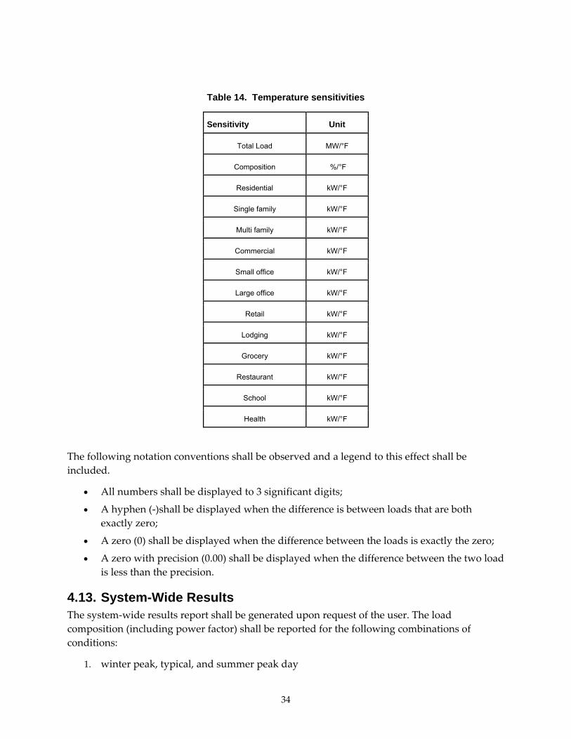
34
Table 14. Temperature sensitivities
Sensitivity Unit
Total Load MW/°F
Composition %/°F
Residential kW/°F
Single family kW/°F
Multi family kW/°F
Commercial kW/°F
Small office kW/°F
Large office kW/°F
Retail kW/°F
Lodging kW/°F
Grocery kW/°F
Restaurant kW/°F
School kW/°F
Health kW/°F
The following notation conventions shall be observed and a legend to this effect shall be
included.
All numbers shall be displayed to 3 significant digits;
A hyphen (‐)shall be displayed when the difference is between loads that are both
exactly zero;
A zero (0) shall be displayed when the difference between the loads is exactly the zero;
A zero with precision (0.00) shall be displayed when the difference between the two load
is less than the precision.
4.13. System-Wide Results The system‐wide results report shall be generated upon request of the user. The load
composition (including power factor) shall be reported for the following combinations of
conditions:
1. winter peak, typical, and summer peak day

35
2. 6 am, 9 am, 3 pm, and 6 pm (note that noon is not included)
3. each city
4. 100% residential, 100% commercial, and 50/50 mixed residential/commercial
All quantities in the report (except for power factor) shall be provided as % of total power.

36

37
5.0 Prototype
A prototype of the tool can be downloaded from SourceForge (SourceForge.net). The tool
provides a numerical reference for validation as well as an illustration of the user input/output
requirements. The prototype shall not be considered an authoritative illustration of what the
tool must do, rather an example of what it can do. It is expected that developers will improve
upon the user interface and data input/output in a substantive way.
5.1. Conditions
Figure 4. The prototype conditions page

38
5.2. Composition
Figure 5. The prototype feeder composition page
Figure 6. The prototype substation composition page

39
5.3. Feeders
Figure 7. The prototype feeder composition table page
5.4. Loadshapes
Figure 8. The prototype loadshapes graphs page

40
5.5. Sensitivity
Figure 9. The prototype sensitivity table page

41
5.6. Residential
Figure 10. The prototype residential single-family design page

42
Figure 11. The prototype residential multi-family design page

43
Figure 12. The prototype residential design page
5.7. Commercial
Figure 13. The prototype commercial design page
5.8. Industrial
Figure 14. The prototype industrial design page

44
5.9. Agricultural
Figure 15. The prototype agricultural design page

45
6.0 References
California End‐use Survey. March 2006. http://capabilities.itron.com/ceusweb/.
Chinn, Garry. ʺModeling Stalled Induction Motors,ʺ presented at the IEEE Transmission and Distribution
Conference. Dallas TX, 2006.
IEEE Task Force on Load Representation for Dynamic Performance. ʺLoad Representation for Dynamic
Performance Analysis.ʺ IEEE Transactions on Power Systems, vol.8, no.2, (1993): 472‐482.
IEEE Task Force on Load Representation for Dynamic Performance. ʺStandard Models for Power Flow and
Dynamic Performance Simulation.ʺ IEEE Transactions on Power Systems, vol.10, no.3, (1995): 1302‐1313.
Kosterev, D., A. Meklin, J. Undrill, B. Lesieutre, W. Price, D. Chassin, R. Bravo, and S. Yang. ʺLoad modeling
in power system studies: WECC progress update.ʺ 2008 IEEE Power and Energy Society General Meeting ‐
Conversion and Delivery of Electrical Energy in the 21st Century, 20‐24. (2008): 1‐8.
NREL TMY2 archive. http://rredc.nrel.gov/solar/old_data/nsrdb/tmy2/.
Pereira, Les, Dmitry Kosterev, Peter Mackin, Donald Davies, John Undrill, and Wenchun Zhu. ʺAn Interim
Dynamic Induction Motor Model for Stability Studies in WSCC.ʺ IEEE Transactions on Power Systems, vol.17,
no.4, (2002): 1108‐1115.
Shaffer, John. ʺAir Conditioner Response to Transmission Faults.ʺ IEEE Transactions on Power Systems, vol.12,
no.2, (1997): 614‐621.
SourceForge.net. http://sourceforge.net/projects/gridlab‐d/files/load‐composition/.
Williams, Bradley, Wayne Schmus, and Douglas Dawson. ʺTransmission Voltage Recovery Delayed by
Stalled Air Conditioner Compressors.ʺ IEEE Transactions on Power Systems, vol.7, no.3, (1992): 1173‐1181.