final project report – poc removal effectiveness of hds units
TRANSCRIPT

Final Project Report – POC Removal Effectiveness of HDS Units 2019
1
Prepared by:
Prepared for:
Prepared by:
FINAL
February 20, 2019
Pollutant of Concern Monitoring for Management Action Effectiveness – Evaluation of Mercury and PCBs Removal Effectiveness of Full Trash Capture Hydrodynamic Separator Units
Project Report
Pollutants of Concern Monitoring for Management Action Effectiveness Evaluation of Mercury and PCBs Removal Effectiveness of Full Trash Capture Hydrodynamic Separator Units
Project Report

Final Project Report – POC Removal Effectiveness of HDS Units 2019
ii
DISCLAIMER
Information contained in BASMAA products is to be considered general guidance and is not to be
construed as specific recommendations for specific cases. BASMAA is not responsible for the use of any
such information for a specific case or for any damages, costs, liabilities or claims resulting from such
use. Users of BASMAA products assume all liability directly or indirectly arising from use of the products.
The mention of commercial products, their source, or their use in connection with information in
BASMAA products is not to be construed as an actual or implied approval, endorsement,
recommendation, or warranty of such product or its use in connection with the information provided by
BASMAA.
This disclaimer is applicable to all BASMAA products, whether information from the BASMAA products is
obtained in hard copy form, electronically, or downloaded from the Internet

Final Project Report – POC Removal Effectiveness of HDS Units 2019
iii
TABLE OF CONTENTS
LIST OF FIGURES ........................................................................................................................................... iv
LIST OF TABLES ............................................................................................................................................. iv
LIST OF ACRONYMS ....................................................................................................................................... v
EXECUTIVE SUMMARY .................................................................................................................................. 1
1 INTRODUCTION ..................................................................................................................................... 5
1.1 Background ................................................................................................................................... 5
1.2 Problem Statement ....................................................................................................................... 6
1.3 Project Goal ................................................................................................................................... 7
2 METHODS .............................................................................................................................................. 9
2.1 Overall Project Approach .............................................................................................................. 9
2.2 HDS Unit Sampling ........................................................................................................................ 9
2.3 Laboratory Methods ................................................................................................................... 10
2.4 Data Analysis and Reporting ....................................................................................................... 11
2.4.1 Annual Mass of POCs Reduced Due to Cleanouts .............................................................. 11 2.4.2 Annual POC Stormwater loads discharged from each HDS Unit Catchment ...................... 13 2.4.3 Evaluation of HDS Unit Performance .................................................................................. 16
3 RESULTS AND DISCUSSION .................................................................................................................. 17
3.1 HDS Unit Sampling ...................................................................................................................... 17
3.1.1 Laboratory Analysis ............................................................................................................. 23 3.2 Evaluation of HDS Unit Performance .......................................................................................... 26
3.2.1 HDS Unit Construction Details and Maintenance Records ................................................. 26 3.2.2 Mass of POCs Removed During Cleanouts .......................................................................... 29 3.2.3 HDS Catchment POC Loads and Calculated Percent Removals Due to Cleanouts .............. 30 3.2.4 Limitations ........................................................................................................................... 32
4 CONCLUSIONS ..................................................................................................................................... 33
5 REFERENCES ........................................................................................................................................ 35
Appendix A: Final Study Design .................................................................................................................. 36
Appendix B: Sampling and Analysis Plan and Quality Assurance Project Plan .......................................... 37
Appendix C: QA Summary Reports ............................................................................................................ 38
Appendix D: PCBs Congeners Concentration Data .................................................................................... 39
Final Project Report – POC Removal Effectiveness of HDS Units 2019
iv
LIST OF FIGURES
Figure 1.1 Basic features of a Contech Continuous Deflective Separator (CDS) Hydrodynamic
Separator (HDS) Unit. Source: Contech Engineered Solutions 2014. 6
Figure 3.1 Catchment Sizes and Land Use Distributions for Existing Public HDS Units in the San
Francisco Bay Area. The HDS units that were sampled in this study are identified with a
black star (sediment-only samples collected) or diamond (sediment/organic debris
samples collected). 17
Figure 3.2 Overview Map of the 8 HDS Units Sampled in the San Francisco Bay Area as Part of the
BASMAA BMP Effectiveness Study. 18
Figure 3.3 Map of HDS Units #1 and #2 Catchments in Sunnyvale, CA. 20
Figure 3.4 Map of HDS Units #3 and #4 Catchments in Oakland, CA 20
Figure 3.5 Map of HDS Unit #5 Catchment in Palo Alto, CA 21
Figure 3.6 Map of HDS Unit #6 Catchment in San Jose, CA 21
Figure 3.7 Map of HDS Unit #7 Catchment in Sunnyvale, CA 22
Figure 3.8 Map of HDS Unit #8 Catchment in San Jose, CA 22
LIST OF TABLES
Table 2.1. Laboratory Analytical Methods for Analytes in Sediment and Sediment/Organic Leaf
debris. ................................................................................................................................... 11
Table 2.2 Land Use-Based PCBs and Mercury Yields. .......................................................................... 14
Table 2.3 Event Mean Concentrations in Water for PCBs and Mercury by Land Use Classification
from the Regional Watershed Spreadsheet Model1. ........................................................... 15
Table 3.1 HDS Units that were sampled in the San Francisco Bay Area as part of the BASMAA POC
Monitoring for Management Action Effectiveness Study.................................................... 19
Table 3.2 Chemical Analysis Results of Solids Collected from HDS Unit Sumps.1................................ 25
Table 3.3 Summary of Information on Storage Capacity, Cleanout Frequencies, and Volumes of
Solids Removed from HDS Unit Sumps. ............................................................................... 27
Table 3.4 PCBs and Mercury Mass Removed During HDS Unit Sump Cleanouts.1 .............................. 29
Table 3.5 HDS Unit Percent Removal of PCBs for Catchment Loads Calculated using Method #1 (Land
use-based Yields) and Method #2 (RWSM Runoff Volume x Concentration).. .................... 30
Table 3.6 HDS unit Percent Removal of Mercury for Catchment Loads Calculated using Method #1
(BASMAA Land use-based Yields) and Method #2 (RWSM Runoff Volume x
Concentration).. ................................................................................................................... 31
Final Project Report – POC Removal Effectiveness of HDS Units 2019
v
LIST OF ACRONYMS
ACCWP Alameda Countywide Clean Water Program
BASMAA Bay Area Stormwater Management Agencies Association
CCCWP Contra Costa Clean Water Program
EPA Environmental Protection Agency
FSURMP Fairfield-Suisun Urban Runoff Management Program
GC/MS Gas Chromatography/Mass Spectroscopy
HDS Hydrodynamic Separator
KLI Kinnetic Laboratories, Inc.
LCS Laboratory Control Sample
MDL Method Detection Limit
MRL Method Reporting Limits
MRP Municipal Regional Stormwater NPDES Permit
MS Matrix Spike
MS4 Municipal Separate Storm Sewer System
na not applicable
nr not reported
ND Non-Detect
NPDES National Pollutant Discharge Elimination System
PCBs Polychlorinated Biphenyl
PMT Project Management Team
POC Pollutants of Concern
ppb parts per billion
ppm parts per million
QA/QC Quality Assurance/Quality Control
QAPP Quality Assurance Project Plan
RWSM Regional Watershed Spreadsheet Model
ROW Right-of-Way
SAP Sampling and Analysis Plan
SCVURPPP Santa Clara Valley Urban Runoff Pollution Prevention Program
SFEI San Francisco Estuary Institute
SMCWPPP San Mateo Countywide Water Pollution Prevention Program
SOP Standard Operating Procedure
TMDL Total Maximum Daily Loads
VSFCD City of Vallejo and the Vallejo Sanitation and Flood Control District

Final Project Report – POC Removal Effectiveness of HDS Units 2019
1
EXECUTIVE SUMMARY
INTRODUCTION The Municipal Regional Stormwater National Pollutant Discharge Elimination System (NPDES) Permit
(MRP; Order No. R2-2015-0049) implements the municipal stormwater portion of the mercury and
polychlorinated biphenyls (PCBs) Total Maximum Daily Loads (TMDLs) for the San Francisco Bay.
Provisions C.11 and C.12 of the MRP require mercury and PCBs load reductions and the development of
a Reasonable Assurance Analysis (RAA) demonstrating that control measures will be sufficient to attain
the TMDL wasteload allocations within specified timeframes. In compliance with the MRP, Permittees
have implemented a number of source control measures in recent years designed to reduce pollutants
of concern (POCs) in urban stormwater and achieve the wasteload allocations described in the mercury
and PCBs TMDLs. For all control measures, an Interim Accounting Methodology for TMDL Loads Reduced
has been developed to determine POC load reductions achieved based on relative mercury and PCBs
yields from different land use categories (BASMAA, 2017a). Provision C.8.f of the MRP further supports
implementation of the mercury and PCBs TMDLs by requiring that Permittees conduct POC monitoring
to address management action effectiveness, one of the five priority information needs identified in the
MRP. Management action effectiveness monitoring is intended to provide support for planning future
management actions or evaluating the effectiveness or impacts of existing management actions.
To achieve compliance with the above permit requirements, the Bay Area Stormwater Management
Agencies Association (BASMAA1) implemented a regional project on behalf of its member agencies. The
goal of the BASMAA POC Monitoring for Management Action Effectiveness -Evaluation of Mercury and
PCBs Removal Effectiveness of Full Trash Capture Hydrodynamic Separator (HDS) Units project (the
Project) was to evaluate the mercury and PCBs removal effectiveness of HDS units associated with
removal of solids captured within the sump. The information provided by this monitoring effort will be
used to support ongoing efforts by MRP Permittees and the California Regional Water Quality Control
Board, San Francisco Bay Region (Regional Water Board) to better quantify the pollutant load reductions
achieved by existing and future HDS units installed in urban watersheds of the Bay Area. This project
was conducted between March 2017 and December 2018 in the portion of the San Francisco Bay Area
subject to the MRP. The project was implemented by a project team comprised of EOA Inc., the Office of
Water Programs at Sacramento State University (OWP), Kinnetic Laboratories, Inc. (KLI), and the San
Francisco Estuary Institute (SFEI). A BASMAA Project Management Team (PMT) consisting of
1 BASMAA is a 501(c)(3) non-profit organization that coordinates and facilitates regional activities of municipal
stormwater programs in the San Francisco Bay Area. BASMAA programs support implementation of the MRP (Order No.
R2-2015-0049). BASMAA is comprised of all 76 identified MRP municipalities and special districts, the Alameda
Countywide Clean Water Program (ACCWP), Contra Costa Clean Water Program (CCCWP), the Santa Clara Valley Urban
Runoff Pollution Prevention Program (SCVURPPP), the San Mateo Countywide Water Pollution Prevention Program
(SMCWPPP), the Fairfield-Suisun Urban Runoff Management Program (FSURMP), the City of Vallejo and the Vallejo
Sanitation and Flood Control District (VSFCD).

Final Project Report – POC Removal Effectiveness of HDS Units 2019
2
representatives from BASMAA stormwater programs and municipalities provided oversight and
guidance to the project team.
METHODS The Project combined sampling and modeling efforts to evaluate the mercury and PCBs removal
performance of HDS units as follows. First, samples of the solids captured and removed from eight
different HDS unit sumps during cleanout were collected and analyzed for PCBs and mercury. Second,
maintenance records and construction plans for these HDS units were reviewed to develop estimates of
the average volume of solids removed per cleanout. This information was combined with the monitoring
data to calculate the mass of POCs removed during cleanouts. Third, the annual mercury and PCBs loads
discharged from each HDS unit catchment were estimated using two different load calculation methods.
Method #1 used the land use-based POC yields described in the BASMAA Interim Accounting
Methodology (BASMAA 2017a) to estimate catchment loads. Method #2 used the Regional Watershed
Spreadsheet Model (RWSM, Wu et al. 2017) to estimate runoff volumes and stormwater concentrations
and calculate catchment loads. Finally, HDS unit performance was evaluated for both catchment load
estimates by calculating the average annual percent removal of POCs as a result of the removal of solids
from the HDS unit sumps.
RESULTS Samples were collected from HDS units located in the cities of Palo Alto, Oakland, San Jose and
Sunnyvale. These HDS units were selected opportunistically, based on the units that were scheduled for
cleanout during the project sampling period (fall 2017 – spring 2018). The types of solid samples that
were collected depended on the solids that were found in each sump, and included 3 sediment-only
samples, and 5 sediment and organic/leafy debris samples. All samples were analyzed for the RMP 40
PCB congeners2, total mercury, total solids (TS), total organic carbon (TOC), and bulk density. The
sediment-only samples were also analyzed for grain size and were sieved at 2 millimeters (mm) prior to
analysis for PCBs and mercury. The sediment and organic/leaf debris samples were analyzed as whole
samples (not sieved) and were also analyzed for total organic matter in order to calculate the inorganic
fraction (i.e., the mineral fraction assumed to be associated with POCs). Total PCBs concentrations
across the 8 samples ranged from 0.01 to 0.41 milligram/kilogram (mg/kg) dry weight (dw). Total
mercury concentrations ranged from 0.005 to 0.31 mg/kg dw. Overall, the range of mercury and PCBs
concentrations measured in the HDS unit solids in the present study were similar to the average
concentrations found in storm drain sediments and street dirt across the Bay Area, as reported
elsewhere (BASMAA 2017a).
Based on review of maintenance records for 38 cleanout events, as well as construction details for each
unit which provided information on each unit’s storage capacity, the estimated average solids removed
per cleanout ranged from 2.4 cubic yards (CY) to 37 CY. These numbers indicate the HDS unit sumps
were on average 97% full when a cleanout was conducted. The calculated annual mass of PCBs removed
2 The 40 individual congeners routinely quantified by the Regional Monitoring Program (RMP) for Water Quality in
San Francisco Bay include: PCBs 8, 18, 28, 31, 33, 44, 49, 52, 56, 60, 66, 70, 74, 87, 95, 97, 99, 101, 105, 110, 118,
128, 132, 138, 141, 149, 151, 153, 156, 158, 170, 174, 177, 180, 183, 187, 194, 195, 201, and 203

Final Project Report – POC Removal Effectiveness of HDS Units 2019
3
from each unit ranged from 2 mg/year up to 2,600 mg/yr, while the annual mass of mercury removed
from each unit ranged from 9 mg/year up to 6,500 mg/year. Differences in catchment sizes do not
explain the high degree of variability observed across the different units. When normalized to
catchment size, the mass of POCs removed per acre treated for the HDS units in this study remained
highly variable, ranging from 0.01 mg/acre to 29 mg/acre for PCBs, and 0.03 mg/acre to 50 mg/acre for
mercury.
PCBs Removal Rates (Table ES-1): For catchment loads calculated using Method #1 (land use-based
yields), the median percent PCBs removal across all 8 units ranged from 5% to 10%. For catchment loads
calculated using Method #2 (RWSM runoff volume x concentration), the median percent PCBs removal
ranged from 15% to 32%. Variability in removal rates was high between individual units, ranging from
almost no removal to 100% removal of the estimated loads.
Table ES-1. HDS Unit Performance - Annual Percent Removal Calculated For Two Catchment Load Estimates.
HDS Unit ID
PCBs Removal Mercury Removal
Method #1 Method #2 Method #1 Method #2
Low High Low High Low High Low High
1 80% 100% 100% 100% 26% 40% 100% 100%
2 8% 18% 10% 22% 4% 6% 65% 98%
3 4% 9% 21% 45% 2% 3% 8% 12%
4 38% 83% 27% 59% 5% 7% 17% 26%
5 0.06% 0.13% 0.21% 0.46% 0.1% 0.2% 1.1% 1.6%
6 5% 11% 20% 43% 0.01% 0.02% 0.1% 0.2%
7 0.6% 1.4% 0.5% 1.1% 0.06% 0.09% 2% 3%
8 1.4% 3.1% 7% 16% 3% 4% 27% 41%
Median 5% 10% 15% 32% 3% 4% 13% 19%
Mercury Removal Rates (Table ES-1): Across all 8 units, the median percent removal for catchment
loads calculated using Method #1 (land use-based yields) ranged from 3% to 4%. For all units under
Method #1, the removal rates were lower for mercury than for PCBs. For catchment loads calculated
using Method #2 (RWSM runoff volume x concentration) the median removal ranged from 13% to 19%.
Similar to PCBs, removal rates for mercury in individual HDS units were highly variable.
CONCLUSIONS For both PCBs and mercury, the data from this study indicate the percent removals achieved by HDS unit
cleanouts are highly variable across units, and likely variable within the same unit over time. The
conclusions on pollutant removal effectiveness of HDS unit sump cleanouts based on the results of this
study are limited by the small number of HDS units that were sampled (n=8) and the limited, and often
incomplete, maintenance records that were available at the time of this study. Nevertheless, the results
of this study provide new information on the range of pollutant concentrations measured in HDS unit
sump solids. Additional data would be needed to fully characterize the range of pollutant load
reductions achieved by HDS units over longer periods of time and across varying urban environments.

Final Project Report – POC Removal Effectiveness of HDS Units 2019
4
The results from this study will be considered in the update of the Interim Accounting Methodology that
is being conducted as part of the BASMAA regional project Source Control Load Reduction Accounting for
Reasonable Assurance Analysis, and will include methods for estimating POC reductions associated with
stormwater control measures, including HDS units.
Additional recommendations on options for potentially improving the pollutant removal effectiveness of
HDS unit maintenance practices, as well as improving the estimates presented in this report include the
following:
Develop site-specific standard operating procedures (SOPs) for each HDS unit, including
suggested cleanout frequency and cleanout methods to ensure efficient and consistent practices
over time.
To improve pollutant removal effectiveness, cleanouts should occur well before sumps reach
capacity. Frequent inspections of HDS unit sumps may also provide the information needed to
determine an appropriate cleanout frequency for each HDS unit.
To improve estimates of the solids removal achieved per cleanout (and the associated pollutant
removals achieved), provide consistent recording of the following information: cleanout dates,
measured depth of solids and water in the sump prior to a cleanout, estimates of the volumes of
solids and water removed from the sump during cleanout, and a description of the types of
solids removed.
Final Project Report – POC Removal Effectiveness of HDS Units 2019
5
1 INTRODUCTION
1.1 BACKGROUND Fish tissue monitoring in San Francisco Bay (Bay) has revealed bioaccumulation of polychlorinated
biphenyls (PCBs) and mercury. The measured fish tissue concentrations are thought to pose a health risk
to people consuming fish caught in the Bay. As a result of these findings, California has issued an interim
advisory on the consumption of fish from the Bay. The advisory led to the Bay being designated as an
impaired water body on the Clean Water Act "Section 303(d) list" due to PCBs and mercury. In response,
the California Regional Water Quality Control Board, San Francisco Bay Region (Regional Water Board)
adopted total maximum daily loads (TMDLs) to address these pollutants of concern (POCs) (SFBRWQCB
2012).
Provisions C.11 and C.12 of the Municipal Regional Stormwater National Pollutant Discharge Elimination
System (NPDES) Permit (MRP; Order No. R2-2015-0049) implements the municipal stormwater portion
of the Mercury and PCBs TMDLs for the San Francisco Bay Area. These provisions require mercury and
PCBs load reductions and the development of a Reasonable Assurance Analysis (RAA) demonstrating
that control measures will be sufficient to attain the TMDL wasteload allocations within specified
timeframes. In compliance with the MRP, Permittees have implemented a number of source control
measures in recent years designed to reduce POCs in urban stormwater and achieve the wasteload
allocations described in the mercury and PCBs TMDLs. For all control measures, the Bay Area
Stormwater Management Agencies Association (BASMAA3) developed an Interim Accounting
Methodology to define POC load reductions achieved based on relative mercury and PCBs yields from
different land use categories (BASMAA 2017a).
Provision C.8.f of the MRP further supports implementation of the mercury and PCBs TMDLs by
requiring that Permittees conduct POC monitoring to address management action effectiveness, one of
the five priority information needs identified in the MRP. Management action effectiveness monitoring
is intended to provide support for planning future management actions or evaluating the effectiveness
or impacts of existing management actions. Although individual Countywide monitoring programs can
meet all MRP monitoring requirements on their own, some requirements are conducted more
efficiently, and likely yield more valuable information, when coordinated and implemented on a regional
basis.
3 BASMAA is a 501(c)(3) non-profit organization that coordinates and facilitates regional activities of municipal
stormwater programs in the San Francisco Bay Area. BASMAA programs support implementation of the MRP
(Order No. R2-2015-0049). BASMAA is comprised of all 76 identified MRP municipalities and special districts, the
Alameda Countywide Clean Water Program (ACCWP), Contra Costa Clean Water Program (CCCWP), the Santa Clara
Valley Urban Runoff Pollution Prevention Program (SCVURPPP), the San Mateo Countywide Water Pollution
Prevention Program (SMCWPPP), the Fairfield-Suisun Urban Runoff Management Program (FSURMP), the City of
Vallejo and the Vallejo Sanitation and Flood Control District (VSFCD).

Final Project Report – POC Removal Effectiveness of HDS Units 2019
6
1.2 PROBLEM STATEMENT During the previous MRP permit term (2009 – 2015), BASMAA pilot tested a number of different
stormwater control measures for pollutant removal effectiveness through the Clean Watersheds for a
Clean Bay (CW4CB) project (BASMAA 2017b). One treatment option that was pilot-tested during CW4CB
includes hydrodynamic separator (HDS) units. HDS units have been installed for trash control
throughout the Bay Area. An HDS unit typically consists of a circular concrete manhole structure that is
installed underground, either inline or offline within the existing storm drainage system. As an example,
the features of an inline Contech Continuous Deflective Separator (CDS) Unit are shown in Figure 1.1.
Stormwater flows from the HDS catchment (up to the treatment design capacity) enter the device
tangentially, which initiates a swirling motion to the water. This is enhanced by a curved deflection
plate. The flows are then guided into the separation chamber, where swirl concentration and screen
deflection force solids to the center of the chamber. The flow continues through the separation screen,
under the oil baffle and exits the unit. All of the solids and debris larger than the screen apertures are
trapped within the unit. Floatables (i.e., buoyant solids) will typically remain suspended in the water that
is retained within the unit near the top of the treatment screen, while the heavier solids settle into the
storage sump located directly below the screening area. These units are designed to collect trash,
sediment and other solid debris. POC removal is expected to occur through capture of POC-containing
solids in the HDS unit sumps, and subsequent removal and disposal of these solids during cleanouts.
Generally, the net solids removal is expected to vary by site-specific conditions, and the removal
efficiency for solids smaller than the screen apertures varies depending on the model selected and the
flow characteristics of the site.
Figure 1.1 Basic features of a Contech Continuous Deflective Separator (CDS) Hydrodynamic Separator (HDS)
Unit. Source: Contech Engineered Solutions 2014.
Final Project Report – POC Removal Effectiveness of HDS Units 2019
7
For HDS units and other stormwater control measures, BASMAA developed the Interim Accounting
Methodology for TMDL Loads Reduced (Interim Accounting Methodology, BASMAA 2017a) to calculate
load reductions achieved by these measures during the current permit term (2016 – 2020). The Interim
Accounting Methodology is based on relative mercury and PCBs yields from different land use
categories. For HDS units, the methodology assumes a default 20% reduction of the area-weighted land
use-based pollutant yields for a given catchment. This default value was based on average percent
removal of total suspended solids (TSS) from HDS units from an analysis of paired influent/effluent data
reported in the International Stormwater Best Management Practices (BMP) Database
(www.bmpdatabase.org), as described in Appendix C of the Interim Accounting Methodology (BASMAA
2017a). However, significant data gaps remain in determining the effectiveness of this practice and
expected load reductions.
The CW4CB results suggested that the materials retained within the HDS unit sumps and removed
during routine cleanouts provide reductions of POC mass that would otherwise remain in the municipal
separate storm sewer system (MS4). However, the CW4CB pilot tests were limited to 2 data points,
collected from a single HDS unit that drains a catchment with elevated mercury and PCBs
concentrations. The monitoring performed to-date is not sufficient to characterize pollutant
concentrations of solids captured in HDS units that drain catchments with different loading scenarios
(e.g., land uses, stormwater volumes, source areas, etc.), nor to estimate the percent removal based on
the pollutant load captured and removed from the HDS unit during ongoing maintenance practices.
1.3 PROJECT GOAL The overall goal of this project is to evaluate the mercury and PCBs removal effectiveness of HDS units
due to solids capture within the sumps and subsequent removal during cleanouts. The monitoring
conducted through this project provides partial fulfilment of MRP monitoring requirements for
management action effectiveness under provision C.8.f., while also addressing some of the data gaps
identified by the CW4CB project (BASMAA 2017b). The information provided by this project will be used
by MRP Permittees and the Regional Water Board to support ongoing efforts to better quantify the
pollutant load reductions achieved by existing and future HDS units installed in urban watersheds of the
Bay Area.
To accomplish the project goal, BASMAA implemented a regional project on behalf of its member
agencies to collect samples of the solids removed from HDS Unit sumps during cleanout events to
estimate the mass of POCs removed. This report presents the results of the BASMAA POC Monitoring
for Management Action Effectiveness - Evaluation of Mercury and PCBs Removal Effectiveness of Full
Trash Capture Hydrodynamic Separator Units project (the Project) that was conducted during 2017 and
2018 in the portion of the San Francisco Bay Area subject to the MRP. The project was implemented by a
project team comprised of EOA Inc., the Office of Water Programs (OWP) at Sacramento State
University, Kinnetic Laboratories, Inc. (KLI), and the San Francisco Estuary Institute (SFEI). A BASMAA
Project Management Team (PMT) consisting of representatives from BASMAA stormwater programs
and municipalities provided oversight and guidance to the project team throughout the project.
Section 2 of this report presents the overall approach and details methods that were used to implement
the project, including a description of the sampling and chemical analysis methods, and descriptions of

Final Project Report – POC Removal Effectiveness of HDS Units 2019
8
the methodology used to estimate the POC percent removals achieved through cleanouts. Section 3
presents the project results and discussion, including the location and description of each HDS unit that
was sampled, a summary of the chemical analysis results for each unit, a summary of the cleanout
events identified in maintenance records, the modeled estimates of the annual average POC stormwater
loads within each HDS unit catchment, and the annual loads reduced (and percent removals achieved)
through HDS unit maintenance practices. Section 4 summarizes the conclusions based on the results of
the project.

Final Project Report – POC Removal Effectiveness of HDS Units 2019
9
2 METHODS
This section presents the overall approach and methods that were used to implement the Project.
Under the guidance and oversight of the PMT, the project team developed a study design (Appendix A)
and a SAP/QAPP (Appendix B), which were followed throughout implementation of the sampling
program.
2.1 OVERALL PROJECT APPROACH The overall approach to the Project involved a combined sampling and modeling effort to evaluate the
mercury and PCBs removal performance of the sampled HDS units. The project implemented the
following 4 tasks:
1. Collect samples of the solids captured in HDS unit sumps in Bay Area urban catchments and
analyze them for mercury and PCBs;
2. Quantify the volume and mass of solids (and associated mercury and PCBs) removed from HDS
unit sumps during cleanouts;
3. Estimate annual average mercury and PCBs stormwater loads for each HDS unit catchment of
interest (i.e., the HDS unit catchments that were sampled in task 1);
4. Calculate the annual mercury and PCBs percent removals due to HDS unit cleanouts for each
catchment of interest.
It is important to note this project was not designed to fully characterize the range of POC
concentrations and masses captured in Bay Area HDS unit sumps. Nor was this project intended to
provide highly accurate stormwater loading estimates for the catchments of interest. Rather, this
project was intended to provide additional data to better quantify the mercury and PCBs load reduction
effectiveness of HDS unit maintenance practices and support future development of source control
RAAs.
The remainder of this section provides additional details on the methods and assumptions employed to
implement the project tasks.
2.2 HDS UNIT SAMPLING Across the Bay Area, at least 37 large, public HDS units have been installed in public right-of-way (ROW)
locations over the past 10+ years. These units were primarily installed for trash controls. These units
treat stormwater runoff from more than 13,000 acres spread across nine Bay Area municipalities. The
size of the catchments treated by individual units in the Bay Area ranges from about 3 acres up to more
than 900 acres. Selection of HDS units for sampling during this project was primarily opportunistic,
based on the units that were scheduled for cleanouts during the project. The project team worked
cooperatively with the PMT and multiple Bay Area municipal agencies to identify public HDS units that
were scheduled for maintenance during the project sampling period (Fall 2017 through spring 2018).
Additional selection criteria included cooperation of the appropriate municipal staff and safety
considerations for the monitoring team. All field sampling was conducted during dry weather, when
urban runoff flows through the HDS units were minimal and did not present safety hazards or other
logistical concerns.

Final Project Report – POC Removal Effectiveness of HDS Units 2019
10
During sampling, HDS units were typically dewatered by municipal staff to remove standing water in the
units and any floatables suspended in that water prior to sump cleanout. The monitoring team then
collected multiple samples of the solids (sediment and organic debris) contained within each unit’s
sump, avoiding trash and other large debris. The solid samples were then combined and thoroughly
homogenized in a stainless steel or Kynar-coated bucket, from which a composite sample was removed
and aliquoted into separate jars for chemical analysis. Sample collection techniques varied between
units due to the unique characteristics of each unit (i.e., sump depth and volume, safety considerations,
etc.). For the majority of units, a stainless steel scoop on the end of a long pole was used to collect
samples of the solids in the sump. However, in cases where the sump was too deep and/or too large to
collect a representative sample using this method, samples were collected after the solids were
removed from the sump by maintenance staff as the cleanout proceeded. Any confined space entry to
remove solids from HDS unit sumps was performed by city maintenance staff trained and certified in
such activities. One composite sample of the solids was collected for each HDS unit. The solid samples
that were collected consisted of either sediment-only, or a combination of sediment and organic/leafy
debris, depending on the type of solids that were found in each sump. The latter type of samples were
collected in cases where this type of material dominated the solids content of the HDS unit sump, and
collection of a sediment-only sample would not be representative of the solids in the sump.
2.3 LABORATORY METHODS All solid samples were analyzed for the RMP 40 PCB congeners4, total mercury, total solids (TS), total
organic carbon (TOC), and bulk density by the methods identified in Table 2.1. All sediment-only samples
were also analyzed for grain size by the methods in Table 2.1. With the exception of grain size and bulk
density, sediment-only samples were sieved by the laboratory at 2 mm prior to analysis. The sediment
and organic/leaf debris samples were not sieved but were analyzed as whole samples. These samples
were also analyzed for total organic matter (TOM) by the method identified in Table 2.1, in order to
estimate the percent of the solid material that was organic (e.g., leaf debris) vs. inorganic (e.g., mineral
content) because POCs in sump solids were assumed to be predominantly associated with the mineral
fraction (i.e., the leafy material is expected to add few POCs but a large contribution to the total solids
mass, and the relative proportion of organic-matter vs. mineral fractions provides assessment of the
degree of dilution by organic matter).
Additional details about the field sampling and laboratory analysis methods are provided in the project
SAP/QAPP (Appendix B).
4 The 40 individual congeners routinely quantified by the Regional Monitoring Program (RMP) for Water Quality in
the San Francisco Estuary include: PCBs 8, 18, 28, 31, 33, 44, 49, 52, 56, 60, 66, 70, 74, 87, 95, 97, 99, 101, 105, 110,
118, 128, 132, 138, 141, 149, 151, 153, 156, 158, 170, 174, 177, 180, 183, 187, 194, 195, 201, and 203
Final Project Report – POC Removal Effectiveness of HDS Units 2019
11
Table 2.1. Laboratory Analytical Methods for Analytes in Sediment and Sediment/Organic Leaf debris.
Sample Type Analyte Sampling Method
Analytical Method Reporting Units
All Total Organic Carbon (TOC)
Grab EPA 415.1, 440.0, 9060, or ASTM D4129M
%
Sediment-Only Grain Size Grab ASTM D422M/PSEP %
All Bulk Density Grab ASTM E1109-86 g/cm3
All Mercury Grab EPA 7471A, 7473, or 1631 µg/kg
All PCBs (RMP 40 Congeners) Grab EPA 1668 µg/kg
All Total Solids Grab EPA160.3 %
Sediment + Organic/Leaf Debris
Total Organic Matter (TOM)
Grab EPA160.4 %
2.4 DATA ANALYSIS AND REPORTING The data collected during sampling was combined with estimated catchment loads to evaluate the POC
removal performance of each HDS unit as follows. First, the annual mass of POCs reduced due to
cleanouts was calculated from the measured POC concentrations in sump solids and the estimated
average volume of solids removed per cleanout, and the total number of cleanouts per year. Next, the
annual stormwater loads of POCs discharged from each HDS unit catchment were estimated using two
different methods to calculate the catchment loads. Finally, HDS unit performance was evaluated by
calculating the POC percent removals due to HDS Unit cleanouts for both catchment load estimates.
Additional details about each of these steps are presented here.
2.4.1 Annual Mass of POCs Reduced Due to Cleanouts
The annual mass of POCs reduced due to removal of sump solids from HDS units during cleanouts was
calculated using Equation 2-1.
(2-1) MHDS-i = VHDS-i x ρHDS-i x FPOC-HDS-i x CPOC, HDS-i x NHDS-i
Where:
MHDS-i the total annual POC mass removed from the sump of HDS Unit i (mg/year);
VHDS-i the volume of solids removed from HDS Unit i during a cleanout (cubic yards
(CY) per cleanout;
ΡHDS-i the bulk density of solids removed from HDS Unit i during a cleanout (kg/CY);
FPOC-HDS-i the mass fraction of solids removed from HDS Unit i during a cleanout that is
associated with POCs;
CPOC, HDS-i the concentration of POCs in the solids removed from HDS Unit i during a
cleanout (mg/kg dw);
NHDS-i the number of cleanouts of HDS Unit i each year (cleanouts/year).

Final Project Report – POC Removal Effectiveness of HDS Units 2019
12
In order to provide the inputs required for Equation 2-1, additional information was gathered from the
appropriate municipalities for each HDS unit that was sampled, including construction details (as-builts)
and maintenance records on past cleanouts. Maintenance records were reviewed to gather information
on the number and frequency of past cleanouts, and the volume of solids typically removed from sumps
during cleanouts. Information on the types of materials removed during each cleanout was generally
limited. However, any cleanout that only recorded removal of floatables (i.e., buoyant solids suspended
in the water layer above the sump) was excluded from these evaluations, as the focus here was on
removal of solid sediment and debris captured in the sumps. Although organic materials such as leaves
are generally buoyant, these solids were frequently found in HDS unit sumps, likely because a sufficient
mass of soil particles attached to the organic debris and caused the materials to settle in the sump.
Additional assumptions described below were used to provide the inputs required for Equation 2-1.
The average volume of solids removed from the sump per cleanout (VHDS-i) was calculated for
each unit from maintenance records or was assumed to be equivalent to the volume of the
unit’s solids storage sump if maintenance records were not available. Where available,
maintenance records were reviewed to identify the volume of solids removed from a given
unit’s sump during each cleanout, and an average volume per cleanout calculated for each unit.
Where not available, construction details (i.e., as-built drawings) were reviewed to calculate the
sump storage capacity for each unit. The full sump capacity was selected as a reasonable
estimate of the volume of solids removed during a cleanout because (1) the recorded volumes
removed during cleanouts were typically near or even exceeded sump capacity; and (2)
information provided by municipal staff indicated solids in the sumps were typically not
removed unless the sumps were well over 50% full. This later information was further
corroborated by maintenance records that identified a number of cleanouts were performed
where only floatables were removed from the top layer of water in the unit’s screening area,
and no solids were removed from the sumps. As stated previously, cleanouts that only removed
these floatables were not included in the calculation of the average volume of solids removed
per cleanout. Initial attempts to further refine and/or improve the estimates of the average
volumes of solids removed per cleanout based on maintenance records were evaluated,
including (for example) normalizing the volume of solids removed in a given cleanout to the
rainfall amounts within that catchment since the previous cleanout. However, because the
maintenance data were limited, highly uncertain, and in many cases, incomplete, the outcomes
of these efforts were inconclusive at best, and they were not pursued further.
The fraction of solids removed during cleanouts that was associated with POCs (FPOC-HDS-i) was
estimated from measurement data for each HDS unit. For sediment-only samples, the fraction
associated with POCs was assumed to be the dry fraction of solids removed that was < 2 mm in
grain size, where %TS accounts for the moisture content of the solids, and the % < 2 mm
accounts for the small particle size fraction of the solids. For the sediment + organic/leaf
samples, the fraction associated with POCs was assumed to be the dry fraction of solids
removed that was inorganic, where % TOM measurement allows for calculation of the %
inorganic (i.e., mineral content of the sample). These assumptions are consistent with
catchment loads calculated in Section 2.4.2 for each HDS unit catchment. Catchment loads

Final Project Report – POC Removal Effectiveness of HDS Units 2019
13
calculated using the BASMAA land use-based POC yields (BASMAA 2017a) or using the Regional
Watershed Spreadsheet Model (RWSM, Wu et al. 2017), both rely on inputs that assume POCs
are associated with the smaller (i.e., < 2 mm) particle size fractions in stormwater.
All of the measurement data used as inputs to Equation 2-1 (POC concentrations, bulk density,
etc.) were assumed to be representative of the values of these parameters for typical sump
solids removed during cleanouts over time for a given HDS Unit. This assumption was necessary
because the data needed to evaluate the temporal and spatial variability in these parameters
are currently unavailable. Multiple samples from the same HDS unit over a number of years
would be needed to quantify the variability over time, while this project provided only 1 sample
per unit. To account for some degree of variability in the measured POC concentrations, the
average relative percent differences (RPDs) between field duplicate sediment samples collected
from storm drain structures over the past 5+ years across the Bay Area were used (SCVURPPP
2018, SMCWPPP 2018, BASMAA 2017b). The RPD was calculated for 27 field duplicate pairs, and
for PCBs, ranged from <1% to 185%, with an average of 37%. For mercury, the RPDs ranged from
4% to 43%, with an average of 17%. The average RPDs for PCBs and mercury were applied to the
concentrations measured in this study to develop a low and high concentration estimate (and
associated low and high POC mass removed per cleanout) for each unit.
Two cleanouts per year were assumed. Although maintenance records provided some
information on cleanout frequencies, it appears from both the information provided, and
further discussion with municipal staff that cleanout frequency is highly variable from unit to
unit and from year to year. A default assumption of two cleanouts per year was selected as a
reasonable approximation based on the typical cleanout frequencies reported by maintenance
staff.
2.4.2 Annual POC Stormwater loads discharged from each HDS Unit Catchment
For each HDS Unit, the annual average POC loads discharged from its catchment were calculated using
two different methods. Method #1 is based on catchment-specific land use multiplied by land use-based
POC yields described in the BASMAA Interim Accounting Methodology (BASMAA 2017a). Method #2 is
based on RWSM estimates of annual stormwater runoff volumes and land use-based POC event mean
concentrations (Wu et al. 2017). Additional details about the inputs and assumptions used to calculate
annual average catchments POC loads using each of these methods are provided below.
2.4.2.1 HDS Catchment Loads – Method #1: BASMAA Land Use-Based Yields
This method relies on the land use-based mercury and PCBs yields that form the basis for the
stormwater control measure load reduction accounting methodology described in the BASMAA Interim
Accounting Methodology (BASMAA 2017a). These yields, presented in Table 2.2, provide an estimate of
the mass of POCs contributed by an area of a given land use each year.

Final Project Report – POC Removal Effectiveness of HDS Units 2019
14
Table 2.2 Land Use-Based PCBs and Mercury Yields.
Land Use Category PCBs Yield
(mg/acre/year) Mercury Yield
(mg/acre/year)
Old Industrial 86.5 1,300
Old Urban 30.3 215
New Urban 3.5 33
Other 3.5 26
Open Space 4.3 33
For each of the HDS Unit catchments in this study, the area of each land use category identified in Table
2.2 was multiplied by the associated POC yield for that land use. The total POC load for each land use
was summed to provide the total POC catchment loads for an average year.
2.4.2.2 HDS Catchment Loads - Method #2: RWSM Runoff Volume X Concentration
For this method, outputs of the RWSM were used to estimate annual average POC loads for each of the
eight HDS unit catchments in this study. The RWSM was developed by SFEI (Wu et al., 2017) to serve as
a regional scale planning tool for estimating average annual loads from small tributaries and sub-
watersheds of San Francisco Bay. The RWSM includes a hydrology model that provides an estimate of
runoff volumes for Bay Area watersheds and sub-watersheds, and pollutant models for PCBs and
mercury that are driven by the hydrology and provide water concentration maps tied to land use
classifications. The hydrology model calculates annual average runoff using rainfall data from PRISM
(Parameter Elevation Regression on Independent Slopes Model, which is based on climate data from
1981 – 2010, www.prismclimate.org), and runoff coefficients developed from land use-soil-slope
combinations. The hydrological calibration was based on 19 watersheds evenly distributed across three
micro-climate sub-regions (East Bay, South Bay/ Peninsula, and North Bay for independent calibrations
that averaged a mean bias of +1%, a median bias of 0% and a range of +/- 30%). One of the outputs from
the model is a continuous estimate of runoff for the entire Bay area in GIS format which can be used to
estimate flow from any spatial extent of interest (parcel, storm, sub-watershed, watershed, sub-region
(e.g. county), or for the Bay area as a whole (Wu et al., 2017). This GIS map was used here to support
this project. The RWSM PCBs and mercury pollutant models were calibrated using data from eight
(PCBs) and six (mercury) well sampled watersheds. The calibration was deemed reasonable for PCBs and
less good for mercury (Wu et al., 2017). One of the outputs from the model provides event mean
concentration (EMC) data for stormwater by land use classification, as shown in Table 2.3.

Final Project Report – POC Removal Effectiveness of HDS Units 2019
15
Table 2.3 Event Mean Concentrations in Water for PCBs and Mercury by Land Use Classification from the Regional Watershed Spreadsheet Model1.
Land Use Classification
Event Mean Concentrations (EMCs)
PCBs ng/L Mercury (ng/L)
Ag and Open Space 0.2
72
New Urban 3
Old Residential 4 63
Old Commercial and Transportation 50
Old Industrial 201 40
Source Areas 1Wu et al. 2017
It is important to note that the land use classifications shown in Table 2.3 are not exactly the same for
PCBs and mercury, nor are they identical for the same pollutant in Tables 2.2 and 2.3. The differences
include the following:
The “old urban” classification in Table 2.2 combines the “old residential” and “old commercial
and transportation” categories for PCBs, while these are distinct categories in Table 2.3;
New Urban, Ag and Open space classifications in Table 2.3 all have the same EMC for PCBs, but
are split into two separate categories (New Urban, and Ag/Open Space) with different EMCs for
mercury, and with different PCBs yields for each category in Table 2.2.
For each HDS Unit catchment in this study, Equation 2-2 was used to calculate the average annual POC
loads for the catchment, using RWSM inputs as described below.
(2-2) MCatchment-i = QCatchment-i x C x EMCCatchment-i
Where:
MCatchment-i the total POC mass discharged from Catchment-i (the catchment draining to
HDS Unit-i) over the time period of interest (mg/year);
QCatchment-i the average annual runoff volume in catchment-i from the RWSM
(liters/year);
C unit conversion factor (ng to mg);
EMCCatchment-i the area-weighted stormwater pollutant event mean concentration (EMC,
ng/l) for Catchment-i based on land use. The RWSM land use-based EMCs in
Table 2.3 (Wu et. al. 2017) were used to calculate an area-weighted
pollutant EMC for each catchment based on the acreage of each land use
classification in the catchment.
Final Project Report – POC Removal Effectiveness of HDS Units 2019
16
2.4.3 Evaluation of HDS Unit Performance
The HDS Unit performance was evaluated by calculating the annual percent removals of POCs due to
cleanout of solids from HDS unit sumps. The percent removal of PCBs and mercury from the total
estimated catchment mass for both of the catchment load estimate methods was calculated using
Equation 2-3.
(2-3) Total Catchment Pollutant Mass Removed (%) = [MHDS-i/MCatchment-i] x 100%
Where:
MHDS-i the total POC mass captured in the sump of HDS Unit i over the time period of
interest (mg/year);
MCatchment-i the total POC mass discharged from Catchment-i (the catchment draining to
HDS Unit-i) over the time period of interest (mg/year) calculated using Method
#1 or Method #2.
Two pollutant percent removals were calculated for each HDS unit catchment using Equation 2-3,
including one for the catchment loads calculated using Method #1 (BASMAA land use-based yields) and
the second for the catchment loads calculated using Method #2 (RWSM runoff volume x concentration).
Final Project Report – POC Removal Effectiveness of HDS Units 2019
17
3 RESULTS AND DISCUSSION
3.1 HDS UNIT SAMPLING Figure 3.1 presents the range of catchment sizes treated by the 37 existing public HDS units in the Bay
Area at the time of this project, and showing the land use distributions of each catchment. The cities of
Oakland, Palo Alto, San Jose, and Sunnyvale all had HDS units that were scheduled for maintenance
during the project period and met the logistical and safety constraints of the project. Between
September 2017 and March 2018, sampling was attempted at 10 HDS units in these cities and competed
successfully at the 8 units identified on Figure 3.1 and on the map in Figure 3.2. Although HDS units were
selected for sampling opportunistically, the HDS units that were sampled span the range of catchment
sizes treated by existing public HDS units in the Bay Area. The majority of HDS unit catchments (both
sampled and not sampled) were dominated by old urban land use.
Additional information about each of the sampled HDS units is presented in Table 3.1. Figures 3.2 - 3.7
provide maps of the catchments for each of the sampled HDS units in this project.
Figure 3.1 Catchment Sizes and Land Use Distributions for Existing Public HDS Units in the San Francisco Bay Area. The HDS units that were sampled in this study are identified with a black star (sediment-only samples collected) or diamond (sediment/organic debris samples collected).

Final Project Report – POC Removal Effectiveness of HDS Units 2019
18
Figure 3.2 Overview Map of the 8 HDS Units Sampled in the San Francisco Bay Area as Part of the BASMAA BMP Effectiveness Study.
Final Project Report – POC Removal Effectiveness of HDS Units 2019
19
Table 3.1 HDS Units that were sampled in the San Francisco Bay Area as part of the BASMAA POC Monitoring for Management Action Effectiveness Study.
HDS ID
Date Installed
HDS Description Lat Long
Land Use Classification (Acres)
Total Area
(Acres) Old
Industrial
Old Urban1 New
Urban Ag/
Open Old
Commercial/Other
Old Residential/
Parks
1 Sep-2014 Mathilda overpass project
CDS1 at California Ave Sunnyvale, CA
37.38224 -122.03306 0.0 0.0 1.5 1.5 0.2 3.3
2 Sep-2014 Mathilda overpass project
CDS2 at Evelyn Ave Sunnyvale, CA
37.37891 -122.03271 1.1 0.3 2.2 3.6 0.0 7.2
3 Aug-2010
HDS 5-G; Perkins & Bellevue (Nature Center)
Oakland, CA 37.80744 -122.25597 0.0 5.3 70.0 0.0 0.0 75.3
4 Jul-2012 HDS 5-D; 22nd and Valley
Oakland, CA 37.81109 -122.26787 1.8 73.2 27.0 0.0 0.3 102.3
5 Jun-2012 W. Meadow Drive and Park
Blvd Palo Alto, CA
37.41816 -122.12538 2.9 17.6 73.9 32.5 0.8 127.5
6 Sep-2012 HDS 604; Sunset Avenue SW
of Alum Rock Avenue San Jose, CA
37.35447 -121.84814 23.0 127.0 441.1 1.6 0.0 592.7
7 Sep-2015 HDS 27A -2 units (East Unit
and West Unit) San Jose, CA
37.38922 -121.99592 269.6 136.2 11.3 282.6 11.9 711.6
8 Jun-2016
HDS 612; Lewis Road and Lone Bluff Way - Los Lagos
Golf Course (2 units) San Jose, CA
37.29923 -121.83591 0.0 171.9 503.2 14.4 53.3 742.8
1The “Old Urban” land use category in the Interim Accounting Methodology (2017a) was further divided into “Old commercial/other” and “Old Urban residential/parks” to provide consistency
with the land use categories in the RWSM (Wu et al. 2017).
Final Project Report – POC Removal Effectiveness of HDS Units 2019
20
Figure 3.3 Map of HDS Units #1 and #2 Catchments in Sunnyvale, CA.
Figure 3.4 Map of HDS Units #3 and #4 Catchments in Oakland, CA
Final Project Report – POC Removal Effectiveness of HDS Units 2019
21
Figure 3.5 Map of HDS Unit #5 Catchment in Palo Alto, CA
Figure 3.6 Map of HDS Unit #6 Catchment in San Jose, CA
Final Project Report – POC Removal Effectiveness of HDS Units 2019
22
Figure 3.7 Map of HDS Unit #7 Catchment in Sunnyvale, CA
Figure 3.8 Map of HDS Unit #8 Catchment in San Jose, CA
Final Project Report – POC Removal Effectiveness of HDS Units 2019
23
3.1.1 Laboratory Analysis
3.1.1.1 Quality Assurance and Quality Control
Data Quality Assurance (QA) and Quality Control (QC) was performed in accordance with the project’s
SAP/QAPP (Appendix B). The SAP/QAPP established Data Quality Objectives (DQOs) to ensure that data
collected are sufficient and of adequate quality for their intended use. These DQOs include both
quantitative and qualitative assessments of the acceptability of data. The qualitative goals include
representativeness and comparability, and the quantitative goals include completeness, sensitivity
(detection and quantization limits), precision, accuracy, and contamination. Measurement Quality
Objectives (MQOs) are the acceptance thresholds or goals for the data.
PCBs: The dataset included 8 field samples, with 3 blanks, and 5 laboratory control samples (LCS), some
in duplicate, meeting the minimum number of QC samples required. Results were reported for the RMP
40 PCB analytes (with their coeluters, yielding 38 unique analytes). One sample was flagged for a hold
time of one week too long but considered unlikely to affect results. Eight of the analytes were detected
in blanks, but field sample concentrations were over 3-fold higher, so no results were censored. Two of
the analytes had recovery with average >35% deviation from target values in the LCS, and one (PCB
183/185) had average error >70%, so was censored. PCB 183/185 was also flagged for poor precision
(RSD 53%), but that analyte was already rejected for poor recovery, so the precision flag is largely moot.
Overall the data quality was acceptable.
Mercury/TOC/TS/bulk density/TOM: The HDS sediment and sediment/organic debris dataset included
eight field samples reported for total mercury, total solids, and bulk density, but only seven for TOC, and
four (missing SJC-604) for sediment/organic debris for total volatile solids (total organic matter, TOM).
MS/D pairs were reported for two sites for TOC, and mercury. Nine lab blanks were reported for
mercury, and 6 for TOC, meeting the one per batch requirement. Three LCSs were also reported for TOC.
Nearly all density and total solids were analyzed past the 1-one week QAPP listed hold times, and
flagged VH, but so long as initial masses were recorded well, it is unlikely to affect results. Only Hg was
occasionally detected in the blanks, but averaged <MDL so results were not flagged. Precision (<25%
RPD) and recovery targets (±20% for conventional analytes and ±25% for Hg) were met for all QC
samples, so no other flags were added. Overall the data quality was acceptable.
Grain Size: The sediment dataset included three field samples reported for grainsize, all analyzed in
replicate. No blanks or recovery samples were reported, which is common for grainsize analysis.
Fourteen size fractions were reported, with results normalized from the raw lab reported percentages to
yield sums of 100% for each analysis. Nominal percent differences in lab replicates for any given sample
were always <5%, so no qualifier flags were added. Overall, the data quality was acceptable.
Additional details about the data quality review are provided in Appendix C. The laboratory QA/QC data
are available upon request.
3.1.1.2 POC Concentrations
Chemical analysis results are summarized in Table 3.2. PCBs concentrations in this report are presented
as the sum of the RMP-40 congeners; individual congener data are available in Appendix D. The
laboratory reports from this project are available upon request. Of the eight samples collected, three

Final Project Report – POC Removal Effectiveness of HDS Units 2019
24
were sediment-only samples that were sieved at 2 mm prior to POC analysis. The remaining five samples
were mixtures of sediment and organic debris (e.g., leaves). These samples were treated as a whole
sample and not sieved at 2 mm prior to POC analysis. Upon consultation with the PMT, the project team
decided to analyze these mixed sediment/organic debris samples as part of this study because these
types of solids (i.e., leaf debris) appeared to be commonly captured in HDS unit sumps.
Total PCBs ranged from 0.01 to 0.41 mg/kg dry weight. The PCBs concentrations observed in the present
study are at least an order of magnitude lower than PCBs concentrations observed in the solids removed
from the 7th Street HDS Unit that drains the Leo Avenue area of San Jose observed in the CW4CB
project in 2013 , where a known source property is located (BASMAA 2017c). Total mercury
concentrations ranged from 0.005 to 0.31 mg/kg dry weight. Overall, the range of mercury and PCBs
concentrations measured in the HDS unit solids in the present study were similar to the average
concentrations found in storm drain sediments and street dirt across the Bay Area, as reported in
Appendix B of the Interim Accounting Methodology (BASMAA 2017a). All laboratory data from this
project are available upon request.

Final Project Report – POC Removal Effectiveness of HDS Units 2019
25
Table 3.2 Chemical Analysis Results of Solids Collected from HDS Unit Sumps.1
HDS Unit ID Sample ID
Sample Date Sample Type
Bulk Density (g/cm3)
Mercury (mg/kg dw)
TOC (%)
Total PCBs (mg/kg dw)
Total Solids
(%)
Total Organic Matter
(%)
Sediment Fraction < 2mm (%)
1 SUN-MatCDS1 3/8/18 Whole-Sediment/
organic debris 0.66 0.11 187 0.053 16.3 53.3 na
2 SUN-MatCDS2 3/8/18 Whole-Sediment/
organic debris 0.57 0.19 283 0.044 13.9 72.6 na
3 OAK-5-G 10/16/17 Sediment Only 0.53 0.25 3.64 0.092 88.5 na 67
4 OAK-5-D 2/2/18 Sediment Only 0.81 0.31 5.85 0.408 99.2 na 95
5 PAL-Meadow 10/25/17 Whole-Sediment/
organic debris 0.47 0.21 222 0.015 19.2 85.4 na
6 SJC-604 10/5/17 Whole-Sediment/
organic debris 0.99 0.04 nr 0.294 10.1 na na
7 SUN-27A 3/8/18 Whole-Sediment/
organic debris 0.76 0.005 375 0.060 8.3 60.3 na
8 SJC-612-01 9/13/17 Sediment Only 0.74 0.14 3.78 0.012 98.3 na 93
1na=not applicable; nr= not reported
Final Project Report – POC Removal Effectiveness of HDS Units 2019
26
3.2 EVALUATION OF HDS UNIT PERFORMANCE
3.2.1 HDS Unit Construction Details and Maintenance Records
Additional information was gathered about each of the sampled HDS units, including construction
details and maintenance records provided by the corresponding municipality. The quantity and quality
of the maintenance records varied greatly from city-to-city and even within a city, from unit to unit.
After careful review of all the available data, relevant information on cleanout frequencies, volumes of
solids removed, and the types of materials contained in the solids was compiled and used to estimate
the volume of solids removed per cleanout (Table 3.3). These data include information on a total of 38
cleanouts at 7 HDS units (2 to 13 cleanouts for each HDS unit in this study with the exception of Palo
Alto, for which no maintenance records were available at the time of this report). In most cases, the
maintenance records provided estimates of the volume of solids removed from the sumps during
cleanouts, as well as the volume of floatables and trash. Both the cities of Sunnyvale and San Jose also
provided the depth of solids in the sump prior to cleanout. This later information was combined with the
known dimensions of each unit’s sump taken from the construction details to calculate the total volume
of solids contained in the sump just prior to cleanout. Some records also provided basic descriptions of
the types of solid materials that were removed from sumps during a cleanout and a rough estimate of
the volume(s) of each type. Excluding cleanouts that only removed floatables, the average volume of
solids removed per cleanout was calculated for each unit and reported in Table 3.3. These estimates
ranged between 2.4 cubic yards (CY) and 37 CY. Interestingly, for five of the HDS units, the volume of
solids removed exceeded the maximum storage capacity of the sumps, indicating solids were likely
overflowing the sump and also contained within the neck and screening area above the sumps of these
units. This suggests sump cleanouts may be needed more frequently at these units, which were typically
cleaned once per year. In contrast, the average solids removed per cleanout for the two Oakland units
ranged from 55% to 60% of the sump capacity, indicating the current cleanout frequency of 2 to 3 times
per year appears adequate for these units.
When normalized to the total area of the catchment, the average volume of solids removed per
cleanout ranged from 0.01 CY to 0.8 CY of solids per acre treated. The solids storage capacity for these 8
units had a similar range of 0.01 CY to 0.7 CY per acre treated. The similarities between measured
storage capacity and estimated solids removed provides further corroboration that, on average,
cleanouts were occurring when the sumps were full. This supports the use of the total sump storage
capacity to represent the volume removed during a cleanout in cases where maintenance data were
unavailable. This also suggests more frequent cleanouts may be warranted.

Final Project Report – POC Removal Effectiveness of HDS Units 2019
27
Table 3.3 Summary of Information on Storage Capacity, Cleanout Frequencies, and Volumes of Solids Removed from HDS Unit Sumps.
HDS Unit ID HDS Catchment Description
Total Storage Capacity
(CY)a
Sump Storage Capacity
(CY)b Cleanout Date
Description of Solids Removed From Unit
Solids Removed per Cleanout (CY)
Average Solids
Removed per Cleanout (CY)
1 Mathilda overpass project CDS1 at California Avenue
4.9 2.2
12/19/2016 leaves/trash/debris 2.5
2.7 8/29/2017 leaves/trash/debris 2.1
10/23/2018 leaves/trash/debris 3.5
2 Mathilda overpass project
CDS2 at Evelyn Ave 3.0 1.5
12/19/2016 leaves/trash/debris 1.8
2.4 8/29/2017 leaves/trash/debris 2.8
10/23/2018 leaves/trash/debris 2.5
3 HDS 5-G; Perkins & Bellvue
(Nature Center) 17 5.8
4/12/2010 60% debris/20% organic/20%trash 2
3.5
5/25/2010 floatables/organic debris 3
7/19/2010 25% sediment/75% Debris 1
2/2/2011 5% floatables/95% organic debris 3
4/25/2011 debris 3
1/12/2012 organic debris and floatables 3
4/18/2012 dirt and debris 1
10/18/2012 sediment debris 12
9/30/2014 sediment/trash 3
5/20/2015 floatables and sediment 3
5/22/2015 floatables and sediment 4
5/19/2017 debris 7
10/18/2017 sediment 1.1
4 HDS 5-D; 22nd and Valley 28 7.3
7/7/2010 dirt/debris/organics 3
4.1
2/4/2011 90% floatables/10% organic debris 4
1/10/2012 dirt/debris/organics 2.5
4/6/2012 dirt/debris/organics 3
10/17/2012 floatables/trash/debris 8
8/27/2013 debris 5
1/27/2015 sediment/trash 1
2/17/2016 sediment/debris 8
4/29/2018 sediment debris 2
Final Project Report – POC Removal Effectiveness of HDS Units 2019
28
Table 3.3 Cont…
HDS Unit ID
HDS Catchment Description
Total Storage Capacity
(CY)a
Sump Storage Capacity
(CY)b Cleanout Date
Description of Solids Removed From Unit
Solids Removed
per Cleanout (CY)
Average Solids
Removed per Cleanout (CY)
5 W. Meadow Dr and Park
Blvd 6.5 1.9 No Maintenance Data Available
6 HDS 604; Sunset Avenue SW of Alum Rock Avenue
31 9.2
9/24/2016 trash/solids 14
10
3/26/2017 trash/solids 9.5
10/5/2017 trash/solids 3.2
12/13/2017 trash/solids 12
3/6/2018 trash/solids 11
7 HDS 27A -2 units (East Unit
and West Unit) 68 18
12/21/2016 leaves/trash/debris 18
10.5 8/30/2017 leaves/trash/debris 4.4
10/25/2018 leaves/trash/debris 8.7
8 HDS 612; Lewis Road and
Lone Bluff Way - Los Lagos Golf Course (2 units)
116 38 9/14/2017 trash/solids 37
37 4/24/2018 trash/solids 37
aThe total storage capacity of each HDS unit was calculated from the dimensions of the solids storage sump and the screening area above the sump, as provided in construction plans. bThe sump storage capacity was calculated from the dimensions of the solids storage sump provided in the construction plans.
Final Project Report – POC Removal Effectiveness of HDS Units 2019
29
3.2.2 Mass of POCs Removed During Cleanouts
The estimated mass of POCs removed during HDS unit sump cleanouts is presented in Table 3.4 for the
following assumed cleanout conditions (i.e., volumes of solids removed during each cleanout):
the average volume of solids removed per cleanout from maintenance records; or
for the Palo Alto HDS Unit #5 only, the volume of solids removed per cleanout was assumed to
be equal to the sump capacity (because no maintenance data were available for this HDS unit);
For each HDS unit, the estimated mass of PCBs removed per cleanout ranged from < 1 mg to > 1,300 mg
of PCBs. If we assume a cleanout rate of twice per year, the calculated mass of PCBs removed per year
from all of these eight HDS units combined ranged from ~2,800 mg to ~6,000 mg of PCBs. When
normalized to the catchment area, the mass of PCBs removed per acre treated ranged from 0.01
mg/acre/yr to 29 mg/acre/yr. The estimated mass of mercury removed per cleanout ranged from ~9 mg
to > 3,200 mg, while the total mass of mercury removed per year from all eight HDS units combined
(again, assuming 2 cleanouts per year) ranged from ~6,300 mg to 9,500 mg. The mass of mercury
removed per acre treated ranged from 0.03 mg/acre/yr to 50 mg/acre/yr. For both PCBs and mercury,
the larger catchments more frequently had lower rates of POCs per acre, although there was not a
consistent correlation between catchment size and the mass of POCs in the sump.
Table 3.4 PCBs and Mercury Mass Removed During HDS Unit Sump Cleanouts.1
HDS Unit ID
Total PCBs Total Mercury
Mass of PCBs per CY of
solids removed
(mg)
Mass of PCBs
removed per
cleanout (mg)
Annual Mass of PCBs
Removed (mg/Year)
Mass of Mercury per CY of
solids removed
(mg)
Mass of Mercury
removed per cleanout
(mg)
Annual Mass of Mercury Removed (mg/Year)
Low High Low High Low High Low High Low High Low High
1 8 17 21 47 43 93 20 30 54 82 109 163
2 3 7 8 17 16 34 18 27 43 65 87 130
3 14 30 49 107 98 213 47 71 167 250 333 500
4 149 325 606 1,318 1,212 2,636 146 218 591 886 1,181 1,772
5 0.5 1.1 1.0 2.1 1.9 4.1 9 13 17 25 33 50
6 48 104 480 1,044 960 2,088 1.0 1.4 9.7 15 19 29
7 9 19 90 197 181 393 11 16 113 170 227 340
8 4 9 147 321 295 641 59 88 2,179 3,268 4,357 6,536
Total Sum 2,807 6,104 Total Sum 6,347 9,520 1The low and high estimates of mass of PCBs and mercury removed were calculated from the measured PCBs and mercury
concentrations in this study and +/- mean RPD of Bay Area sediment PCBs concentrations of +/- 37% (PCBs) and +/- 17%
(mercury), as described in Section 2.4.1.

Final Project Report – POC Removal Effectiveness of HDS Units 2019
30
3.2.3 HDS Catchment POC Loads and Calculated Percent Removals Due to Cleanouts
The annual POC loads discharged from each HDS Unit catchment calculated using Method #1 and
Method #2, along with the calculated percent removals are presented in Tables 3.5 and 3.6 for PCBs and
mercury, respectively. For the purpose of calculating descriptive statistics, percent removal was capped
at 100%.
Table 3.5 HDS Unit Percent Removal of PCBs for Catchment Loads Calculated using Method #1 (Land use-based Yields) and Method #2 (RWSM Runoff Volume x Concentration).
HDS Unit ID
Method #1 Catchment Load Land Use-Based Yields
Method #2 Catchment Load RWSM Runoff Volume x Concentration
HDS Catchment Info
HDS Performance Annual Percent
Removal HDS Catchment Info
HDS Performance Annual Percent
Removal
PCBs Yield (mg/acre/yr)
PCBs Load (mg/yr) Low High
PCBs Yield (mg/acre/yr)
PCBs Load (mg/yr) Low High
1 16 53 80% 100% 3 9 100% 100%
2 26 187 8% 18% 22 158 10% 22%
3 30 2,281 4% 9% 6 478 21% 45%
4 31 3,192 38% 83% 44 4,478 27% 59%
5 25 3,135 0.06% 0.13% 7 898 0.2% 0.5%
6 32 19,209 5% 11% 8 4,832 20% 43%
7 41 28,828 0.6% 1.4% 49 34,806 0.5% 1.1%
8 28 20,735 1.4% 3.1% 5 3,997 7% 16%
Median 29 3,164 5% 10% 8 2,447 15% 32%
Range 16 - 41 53 - 28,828 0.06% 100% 3 - 49 9 - 34,806 0.2% 100%
With the catchment loads calculated using Method #1, the PCBs percent removal varied greatly
between HDS units, ranging from a low of <1% removal to a high of 100% removal. The median percent
removal across all 8 units ranged from 5% to 10%.
With the catchment loads calculated using Method #2, the PCBs percent removal also varied greatly
between HDS units, ranging from a low of <1% removal to a high of 100% removal. However, the
median removal rate across all eight units was higher, ranging from 15% to 32%. Again, the variability in
removal rates between individual HDS units was high. Generally, the percent removals were lower for a
given HDS unit when the catchment loads were calculated using Method #1 compared with Method #2.
Only HDS Unit #4 had a higher percent removal under Method #1.

Final Project Report – POC Removal Effectiveness of HDS Units 2019
31
Table 3.6 HDS unit Percent Removal of Mercury for Catchment Loads Calculated using Method #1 (BASMAA Land use-based Yields) and Method #2 (RWSM Runoff Volume x Concentration).
HDS Unit ID
Catchment Load for Method #1 BASMAA Land Use-Based Sediment Yields
Catchment Load for Method #2 RWSM Runoff Volume x Concentration
HDS Catchment Info
HDS Performance Annual Percent
Removal HDS Catchment Info
HDS Performance Annual Percent
Removal
Mercury Yield
(mg/acre/yr)
Mercury Load
(mg/yr) Low High
Mercury Yield
(mg/acre/yr)
Mercury Load
(mg/yr) Low High
1 126 412 26% 40% 21.0 69 100% 100%
2 297 2,140 4% 6% 18.4 133 65% 98%
3 215 16,188 2% 3% 55.4 4,174 8% 12%
4 233 23,876 5% 7% 67.7 6,928 17% 26%
5 192 24,479 0.14% 0.20% 23.9 3,055 1.1% 1.6%
6 257 152,118 0.01% 0.02% 23.5 13,922 0.1% 0.2%
7 551 391,874 0.06% 0.09% 16.8 11,940 1.9% 2.8%
8 198 147,379 2% 3% 21.7 16,084 27% 41%
Median 224 24,177 2% 3% 23 5,551 13% 19%
Range 126 - 551 412-391,874 0.01% 40% 21 - 68 69 - 16,084 0.13% 100%
For mercury, the removal rates for catchment loads calculated using Method #1 ranged from 0.01% to
40% removal, and the median percent removal across all eight units ranged from 2% to 3%. The
mercury removal rates for catchment loads calculated using Method #2 ranged from a low of <1%
removal to a high of 100% removal. The median removal rate across all 8 units ranged from 13% to 19%.
These results show the percent of mercury capture for both catchment load calculation methods was
typically lower than for PCBs, which is consistent with observations in other studies of BMP
effectiveness in the Bay Area (Gilbreath et al. 2019, David et al. 2015, Yee and McKee 2010).
One notable difference between the catchment load calculation methods presented in Tables 3.5 and
3.6 is that the catchment-specific yields (POC mass per acre per year) calculated for the same HDS unit
catchment under each method are substantially different. The RPDs for the paired catchment-specific
yields calculated under Scenario 1 and Scenario 2 ranged from 3% to 67%, with an average of 39% for
PCBs. Also, for PCBs the differences in catchment yields for a given unit were not consistently higher or
lower for Method #1 vs. Method #2 catchment load estimates. The RPDs between catchment yields
under the 2 loading scenarios for each HDS unit were generally larger for mercury, ranging from 47% to
90%, with an average of 68%.
Overall, the results of this study indicate the HDS unit performance appears to vary substantially
between units, regardless of the method used to estimate the catchment loads. Even when normalized
to the area of the HDS unit catchment, the POCs removed per acre treated were highly variable between
units, ranging up to over a thousand fold difference between the highest and lowest capture rates. The
method used to calculate the catchment annual loads also impacts the calculated performance of the
individual HDS units.

Final Project Report – POC Removal Effectiveness of HDS Units 2019
32
3.2.4 Limitations
It is important to note, that all of the assumptions that were used in the calculations described in this
report represent important limitations of this study and highlight the paucity of data that are currently
available to evaluate HDS Unit performance for PCBs and mercury removals. Although this study
provided new data on the concentrations of POCs in the solids removed from HDS unit sumps during
cleanouts, the data set remains small (n=8), especially in comparison to the expected (and observed)
variability between each unit. The calculated removal rates, even under the same loading scenario, were
highly variable across different HDS Units, ranging from almost zero POC removal, to 100% removal of all
POCs discharged from the catchment. Although an estimate of variability in POC concentrations was
applied based on information about the variability in street dirt and storm drain sediments, the authors
of this report acknowledge this estimated variability likely falls far short of accounting for the full range
of variability and error in the input parameters used to calculate the POC removal rates presented here.
Much more data would be needed to improve these estimates and better characterize the true
variability in removal rates between units, and within the same unit over time.
One data input that proved particularly difficult to account for was the volume of solids (and associated
mass) that was removed from HDS units during each cleanout. This study relied on the limited
information recorded in maintenance records provided by individual cities for each of the HDS units in
this study. The information that was provided varied from cleanout to cleanout, and from city to city.
Although some cities provided measurements of the depth of solids in a unit at cleanout, which allowed
a more accurate calculation of the total solids volume, in many cases, the information provided was
likely based on a visual assessment by the maintenance staff onsite at the time of the cleanout, and thus
subject to a large degree of error.
Nevertheless, this study increased the number of data points on POC concentrations in the solids
removed from HDS Unit sumps during cleanouts from n=2 (the Leo Ave HDS data from CW4CB) to n=10,
an increase of 500%. Furthermore, because of the careful review of maintenance records that was
performed as part of this study, the authors were able to identify a number of recommendations
(provided in Section 4) for improving the removal effectiveness of HDS unit maintenance practices, and
improving the quality of maintenance records for the purpose of quantifying solids removed, and. the
volume of solids associated with pollutants.
Final Project Report – POC Removal Effectiveness of HDS Units 2019
33
4 CONCLUSIONS
The Project combined sampling and modeling efforts to evaluate the mercury and PCBs removal
performance of HDS units. Samples of the solids captured in 8 HDS units in the Bay Area were collected
and analyzed for PCBs and mercury. The monitoring data collected by this project provided partial
fulfilment of MRP monitoring requirements for management action effectiveness under provision C.8.f.,
and also addressed some of the data gaps on BMP effectiveness that were identified by the CW4CB
project (BASMAA, 2017b). This study also reviewed information on HDS Unit maintenance practices,
including the frequency of cleanouts, the volumes of solids removed during these cleanouts, and the
types of materials contained within the solids. This information was used to develop estimates of the
average solids removal per cleanout, and combined with concentration data, the mass of mercury and
PCBs removed per cleanout. Finally, the percent removals achieved by HDS unit cleanouts were
calculated using two different methods to estimate the catchment loads, including BASMAA land use-
based pollutant yields (BASMAA 2017a), and RWSM runoff-concentration load estimates (Wu et al.
2017).
Based on median values, the results of this study suggest HDS unit maintenance practices reduce loads
of PCBs from 5% to 32%, while mercury load reductions are lower, ranging from 3% to 19%. For both
PCBs and mercury, the data from this study demonstrate the percent removals achieved by HDS unit
cleanouts are highly variable across units, and likely variable within the same unit over time.
The conclusions on pollutant removal effectiveness of HDS unit sump cleanouts based on the results of
this study are limited by the small number of HDS units that were sampled (n=8) and the limited, and
often incomplete, maintenance records that were available at the time of this study. Nevertheless, the
results of this study provide new information on the range of pollutant concentrations measured in HDS
unit sump solids. Much more data would be needed to fully characterize the range of pollutant load
reductions achieved by HDS units over longer periods of time and across varying urban environments.
In addition to the conclusions above, this study also identified the following suggestions for potentially
increasing the PCBs and mercury removal effectiveness of HDS unit maintenance practices, and to
improve the quality of the data available for calculating loads reduced. First, review of maintenance
records indicated that the HDS unit sumps were often full or nearly full when the cleanouts occurred.
Because no pollutant removal can occur after the sumps are 100% full, conducting cleanouts well before
capacity is reached would likely improve pollutant removal rates for a given unit. However, given the
site-specific nature of sump loading and variability across time, both the cleanout frequency and the
cleanout methods required are likely to be highly site-specific. Development of site-specific standard
operating procedures (SOPs) for cleanout frequency and cleanout methods for each HDS unit may be
needed to ensure efficient and consistent practices over time. Frequent inspections of HDS unit sumps
may also provide the information needed to determine an appropriate cleanout frequency for each HDS
unit.
Second, review of maintenance records highlighted the need for more detailed and consistent reporting
on each cleanout. The maintenance records provided by municipalities in this study varied considerably
in the quantity and quality of the information provided. The variability was high both between cities,
Final Project Report – POC Removal Effectiveness of HDS Units 2019
34
and within cities for the same unit over time. To improve estimates of the solids removal achieved per
cleanout (and the associated pollutant removals achieved), consistent recording of the following
information for each cleanout would be useful.
o cleanout date
o measured depth of solids in the sump prior to cleanout;
o measured depth of water in the sump prior to cleanout;
o an estimate of the volume of water removed during the cleanout;
o an estimate of the volume of solids removed during the cleanout;
o a description of the materials contained in the sump solids – including estimates of the
percent contribution by volume of sediment, organic materials (leaves and vegetation),
trash and large debris, and floatables;
o clearly identify all cleanouts that ONLY remove floatables;
The information above would provide better estimates of the solids removed per cleanout, and a better
understanding of the solids captured in HDS units that are likely associated with POCs. Both pieces of
information are important for improving estimates of pollutant removal effectiveness of HDS unit
cleanouts. This information could also be reviewed periodically to determine if the appropriate cleanout
frequencies are being maintained.

Final Project Report – POC Removal Effectiveness of HDS Units 2019
35
5 REFERENCES
BASMAA, 2017a. Interim Accounting Methodology for TMDL Loads Reduced. Bay Area Stormwater
Management Agencies Association.
BASMAA, 2017b. Clean Watersheds for a Clean Bay Project Report, Final Report May 2017. Bay Area
Stormwater Management Agencies Association.
BASMAA, 2017c. Clean Watersheds for a Clean Bay Task 5: Stormwater Treatment Retrofit Pilot Projects
- 7th Street Hydrodynamic Separator Unit draining the Leo Avenue Watershed, San Jose, CA.
Bay Area Stormwater Management Agencies Association.
Contech Engineered Solutions LLC, 2014. CDS Guide: Operation, Design, Performance and Maintenance.
Available at www.conteces.com.
David, N., Leatherbarrow, J.E, Yee, D., and McKee, L.J, 2015. Removal Efficiencies of a Bioretention
System for Trace Metals, PCBs, PAHs, and Dioxins in a Semi-arid Environment. Journal of
Environmental Engineering, 141(6) (June).
Gilbreath, A.N, McKee, L.J., Shimabuku, I., Lin D., Werbowski, L.M., Zhu, X., Grbic, J., Rochman, C., 2019
(accepted). Multi-year water quality performance and mass accumulation of PCBs, mercury,
methylmercury, copper and microplastics in a bioretention rain garden. Journal of Sustainable
Water in the Built Environment.
Santa Clara County, 2007. Santa Clara County California Drainage Manual 2007. Prepared by Schaaf &
Wheeler for Santa Clara County. August 14, 2007.
SCVURPPP, 2018. Pollutants of Concern Monitoring Data Report. Water Year 2017. Santa Clara Valley
Urban Runoff Prevention Program. March 31, 2018.
SFBRWQCB, 2012. San Francisco Bay Regional Water Quality Control Board. Total Maximum Daily Loads
(TMDLs) and the 303(d) List of Impaired Water Bodies. 2012.
SFBRWQCB, 2015. Municipal Regional Stormwater NPDES Permit, Order No. R2-2015-0049. NPDES
Permit No. CAS612008. November 19, 2015
SMCWPPP, 2018. Pollutants of Concern Monitoring Data Report. Water Year 2017. San Mateo
Countywide Water Pollution Prevention Program. March 29, 2018.
Wu, J; Gilbreath, A.; McKee, L. J. 2017. Regional Watershed Spreadsheet Model (RWSM): Year 6 Progress
Report. SFEI Contribution No. 811. San Francisco Estuary Institute: Richmond, CA.
Yee, D., and McKee, L.J., 2010. Task 3.5: Concentrations of PCBs and Hg in soils, sediments and water in
the urbanized Bay Area: Implications for best management. A technical report of the Watershed
Program. SFEI Contribution 608. San Francisco Estuary Institute, Oakland CA 94621. 36 pp. +
appendix. http://www.sfei.org/documents/concentrations-pcbs-and-hg-soils-sediments-and-
water-urbanized-bay-area-implications-best.

Final Project Report – POC Removal Effectiveness of HDS Units 2019
APPENDIX A: FINAL STUDY DESIGN
POC Monitoring for
Management Action Effectiveness
Monitoring Study Design Final, September 2017
Prepared for:
Prepared by:
1410 Jackson Street 6000 J Street 4911 Central Avenue 307 Washington Street Oakland, California Sacramento, California Richmond, California Santa Cruz, California 94612 95819 94804 95060

Contents List of Tables ....................................................................................................................... 3 List of Figures ...................................................................................................................... 3
1. Introduction .......................................................................................................................... 4 2. Problem Definition ............................................................................................................... 5
2.1 HDS Units ............................................................................................................... 5 2.2 Bioretention ............................................................................................................ 7
3. Study Goals ....................................................................................................................... 10 3.1 Primary Management Questions .......................................................................... 10 3.2 Secondary Management Questions ..................................................................... 10 3.3 Level of Confidence .............................................................................................. 11
4. Study Design Options ........................................................................................................ 12 4.1 Influent-Effluent Monitoring ................................................................................... 13 4.2 Sediment Sampling .............................................................................................. 14
4.3 Before-After Monitoring ........................................................................................ 15 5. Primary Data Objectives .................................................................................................... 16
5.1 Data Objective 1: Annual Loads Captured by HDS Units ..................................... 16
5.2 Data Objective 2: Loads Reduced by Biochar-Amended BSM ............................. 16 6. BMP Processes and Key Study Variables ......................................................................... 18
6.1 HDS Units ............................................................................................................. 19 6.2 Bioretention .......................................................................................................... 20
7. Monitoring and Sampling Options ...................................................................................... 21
7.1 HDS Units ............................................................................................................. 21
7.1.1 Influent Quality ..................................................................................................... 21 7.1.2 BMP Design and Hydraulic Loading .................................................................... 24 7.1.3 Operation and Maintenance ................................................................................ 26 7.2 Enhanced Bioretention ......................................................................................... 26
7.2.1 Influent Quality ..................................................................................................... 26 7.2.2 BMP Design and Hydraulic Loading .................................................................... 27
7.2.3 Media Type and Properties.................................................................................. 27 7.2.4 Operation and Maintenance Parameters ............................................................. 29 7.3 Uncontrolled Variables and Study Assumptions ................................................... 29
8. Final Study Design ............................................................................................................ 31 8.1 Statistical Testing & Sample Size ......................................................................... 31
8.2 Constituents for Sediment Analysis ...................................................................... 31
1 – Only total mercury analyzed. Methyl mercury is not ................................................... 32 relevant for SF Bay TMDL. ................................................................................................ 32 8.3 Constituents for Water Quality Analysis................................................................ 32 1 – Only total mercury analyzed. Methyl mercury is not ................................................... 33 relevant for SF Bay TMDL. ................................................................................................ 33 8.4 Budget and Schedule ........................................................................................... 33
8.5 Optimized Study Design ....................................................................................... 33 8.6 Adequacy of Study Design ................................................................................... 37
9. Recommendations for Sampling and Analysis Plans......................................................... 39
9.1 HDS Monitoring .................................................................................................... 39
9.2 Enhanced Bioretention Media Testing .................................................................. 39 9.3 Data Quality Objectives ........................................................................................ 40
10. References ........................................................................................................................ 41
List of Tables
Table 2.1 Summary of Data Collected from Leo Avenue HDS during October, 2014 Annual Cleanout Event ................................................................................................................................ 6
Table 2.2 Summary of Bay Area Drain Inlet Sediment Concentration Data ......................... 6
Table 7.1 HDS Sampling Design based on Watershed Land Use ........................................ 22
Table 7.2 Percent of Land Use in HDS Watershed Areas .................................................... 23
Table 7.3 HDS Sampling Design based on Predominant Land Use ..................................... 24
Table 7.4 HDS Sampling Design based on Predominant Land Use and HDS Size ............... 25
Table 7.5 Example Sampling Design for Laboratory Column Experiments ........................ 28
Table 8.1 Selected Constituents for HDS Sediment Monitoring ........................................ 32
Table 8.2 Selected Aqueous Constituents for Media Testing in Laboratory Columns ....... 33
Table 8.3 HDS Monitoring Study Design ............................................................................. 35
Table 8.4 Enhanced BSM Testing Study Design .................................................................. 36
List of Figures
Figure 2.1 Cumulative Frequency Distribution of Total PBCs Influent Concentrations for Bioretention Media with and without Biochar ............................................................................... 8
Figure 4.1 Typical BMP system and pollutant pathways .................................................... 12
Figure 4.2 Comparison of two hypothetical non-overlapping BMP regressions ................ 14
Figure 7.1 Land Use based PCB and Mercury Loading based on BASMAA Integrated Monitoring Reports (SFEI, 2015) ................................................................................................... 22

Page 4
1. Introduction Discharges of PCBs and mercury in stormwater have caused impairment to the San
Francisco Bay estuary. In response, the Regional Water Board adopted total maximum daily loads (TMDLs) to address these pollutants of concern (POC) (SFBRWQCB, 2012). Provisions C.11 and C.12 the Municipal Regional Stormwater NPDES Permit, MRP (SFBRWQCB, 2015) implement the Mercury and PCB Total Maximum Daily Loads (TMDLs) for the San Francisco Bay Area. These provisions require mercury and PCB load reductions and the development of a Reasonable Assurance Analysis (RAA) demonstrating that control measures will be sufficient to attain the TMDL waste load allocations within specified timeframes. Provision C.8.f of the MRP supports implementation of the mercury and PCB TMDLs provisions by requiring that Permittees conduct pollutants of concern (POC) monitoring to address the five priority information needs listed below.
1. Source Identification – identifying which sources or watershed source areas provide the greatest opportunities for reductions of POCs in urban stormwater runoff;
2. Contributions to Bay Impairment – identifying which watershed source areas contribute most to the impairment of San Francisco Bay beneficial uses (due to source intensity and sensitivity of discharge location);
3. Management Action Effectiveness – providing support for planning future management actions or evaluating the effectiveness or impacts of existing management actions;
4. Loads and Status – providing information on POC loads, concentrations, and presence in local tributaries or urban stormwater discharges; and
5. Trends – evaluating trends in POC loading to the Bay and POC concentrations in urban stormwater discharges or local tributaries over time.
Table 8.2 of Provision C.8.f identifies the minimum number of samples that each MRP Countywide Program (i.e., Santa Clara, San Mateo, Alameda, and Contra Costa) must collect and analyze to address each monitoring priority. Although individual Countywide monitoring programs can meet these monitoring requirements, some requirements can be conducted more efficiently and will likely yield more valuable information if coordinated and implemented on a regional basis. The minimum of eight (8) PCB and mercury samples required by each Program to address information priority #3 is one such example. Findings from a regionally-coordinated monitoring effort would better support development of the RAA.
This Study Design describes monitoring and sample collection activities designed to meet the requirements of information priority #3 of Provision C.8.f of the MRP. The activities planned include field sampling of hydrodynamic separators and laboratory experiments with amended bioretention soils. Study planning is important to ensure that the right type of data are collected and there is a sufficient sample size and power to help address the management questions within the available time and budget constraints. Essential components of the study plan include describing problems, defining study goals, identifying important study parameters, specifying methodologies, and validating and optimizing the study design.
Page 5
2. Problem Definition Studies conducted to date have identified PCB source areas in the Bay Area where
pollutant management options may be feasible and beneficial. Enhanced municipal operational PCB management options (e.g., street sweeping, storm drain line cleanout) have the advantage of being familiar and well-practiced, address multiple benefits, and the cost-benefit may exceed that for stormwater treatment (BASMAA, 2017a). Site-specific stormwater treatment via bioretention, however, is now commonly implemented to meet new and redevelopment (MRP Provision C.3) requirements. An added benefit of redevelopment is that PCB-laden sediment sources can be immobilized. However, many areas where certain land uses or activities generate higher PCB concentrations in runoff are unlikely to undergo near-term redevelopment, and instead may only be subject to maintenance operations or stormwater BMP retrofit projects implemented by the municipality. Consequently it is valuable to maximize cost effective PCB removal benefit of both operations and maintenance, and stormwater treatment.
Two treatment options that have the potential to reduce PCB discharges include hydrodynamic separators (HDS units) and enhanced bioretention filters. These options were pilot-tested in the Clean Watersheds for a Clean Bay (CW4CB) Project (BASMAA, 2017a). HDS units are being implemented for trash control throughout the Bay Area and collect sediment to some extent along with trash and other debris. Quantifying PCB mass removed by these units will help MRP Permittees account for the associated load reductions. For these and other control measures, an Interim Accounting Methodology has been developed based on relative mercury and PCBs yields from different land use categories (BASMAA, 2017c). Bioretention is a common treatment practice for new development and redevelopment in the San Francisco Bay Area, so enhancing the performance of bioretention is also attractive.
At this time reducing mercury loads in stormwater runoff is a lower priority than PCBs load reduction. The assumption during the MRP 2.0 permit term is that actions taken to reduce PCBs loads in stormwater runoff are generally sufficient to address mercury. Therefore, optimizing stormwater controls for PCBs is the primary focus in this study.
2.1 HDS Units
Limited CW4CB monitoring conducted at two HDS sites was used to calculate the mass of PCBs in trapped sediment (BASMAA, 2017a). The two sites sampled were Leo Avenue in San Jose and City of Oakland Alameda and High Street. The Leo Avenue HDS unit treats runoff from approximately 178 acres of watershed with a long history of industrial land uses, including auto repair and salvage yards, metal recyclers, and historic rail lines. The City of Oakland Alameda and High Street HDS has a tributary drainage area of approximately 35 acres with a high concentration of old industrial and commercial land uses, including historic rail lines.
Sampling of the two CW4CB HDS units was opportunistic and associated with scheduled cleanouts. Two sump cleanout events took place in August 2013, one at the Leo Avenue HDS unit and one at the Alameda and High Street HDS unit. However, due to a lack of captured sediment the samples collected were aqueous phase samples instead of sediment samples. An additional cleanout took place at Leo Avenue in October 2014. A sump sediment sample

Page 6
collected and analyzed during this cleanout contained total PCB concentrations of 1.5 mg/kg and mercury concentrations of 0.33 mg/kg for sediment less than 2 mm in size, and estimated annual total PCB and mercury removals were 375 mg and 82.4 mg, respectively (Table 2.1). The HDS sediment concentrations are comparable to previous Leo Avenue watershed measurements in sediments from piping assessed via manholes, drop inlets/catch basins, streets/gutters, and private properties (ND to 27 mg/kg for PCBs and 0.089 to 6.2 mg/kg for mercury) (BASMAA, 2014). At the Alameda and High Street HDS unit, tidal influences of Bay water prevented additional monitoring.
Table 2.1 Summary of Data Collected from Leo Avenue HDS during October, 2014 Annual Cleanout Event
There are no known published studies characterizing HDS sediment for PCBs or mercury, so the Leo Avenue results are compared to relevant drain inlet/catch basin sediment studies. In the Bay Area, different municipalities have collected and analyzed drain inlet cleaning sediment samples. The analytical results for these drain inlet sediment samples are summarized in Table 2.2 (BASMAA, 2014). As can be seen from Table 2.2, the Leo Avenue sediment PCB concentrations are higher than those measured in Bay Area drain inlet sediment by up to an order-of-magnitude, but mercury concentrations are comparable.
Table 2.2 Summary of Bay Area Drain Inlet Sediment Concentration Data
(Based on readily available data; see BASMAA (2016b) for additional summaries for street and storm drain sediment)

Page 7
Monitoring by the City of Spokane, Washington, showed total PCBs in catch basin sediment ranged between 0.025 mg/kg and 1.7 mg/kg for an industrial area with known PCB contamination (City of Spokane, 2015). A City of San Diego study characterized sediments in eight catch basins in a 9.5 acre area of downtown San Diego classified as high density mixed use with roads, sidewalks, and parking lots (City of San Diego, 2012). Concentrations of common aroclors in the catch basin sediments varied from about 0.040 to over 0.9 mg/kg. Monitoring by the City of Tacoma showed PCB concentrations in stormwater sediment traps varied from nondetect to a maximum near 2 mg/kg (City of Tacoma, 2015). The highest PCB concentrations in catch basin sediments ranged from 16 mg/kg in downtown Tacoma to 18 mg/kg in East Tacoma. These published drain inlet/catch basin studies show that PCB and mercury concentrations can vary substantially in storm drain sediments depending on the characteristics of the watershed.
Sampling of captured sediment at the Leo Avenue HDS in San Jose highlighted the potential of HDS maintenance as a management practice for controlling PCB and mercury loads. The BASMAA Interim Accounting Methodology that is currently being used to calculate load reductions assumes a default 20% reduction of the area-weighted land-used based pollutant yields for a given catchment. This default value was based on average percent removal of TSS from HDS units based on analysis of paired influent/effluent data. However, significant data gaps remain in determining the effectiveness of this practice and expected load reductions. HDS sediment sampling has been limited to a few samples. PCB concentrations in the Leo Avenue HDS sample were much higher than average concentrations in Bay Area drain inlet sediment. Drain inlet/catch basin sediment sampling by others suggests that sediment PCB and mercury concentrations can vary substantially from watershed to watershed. The monitoring performed to date is not sufficient to characterize pollutant concentrations of sediment captured in HDS units that drain catchments with different loading scenarios (e.g., land-uses, stormwater volumes, etc.), nor to estimate the percent removal based on the pollutant load captured by the HDS unit. Additional sampling is needed to better quantify the PCB and mercury loads capture by these devices, and calculate the percent removal achieved. Consequently, quantification of PCBs removed at other HDS locations and evaluation of the percent load reduction achieved is needed to provide better estimates of PCB load reductions from existing HDS unit maintenance practices.
2.2 Bioretention
The results of monitoring the performance of bioretention soil media (BSM) amended with biochar at one CW4CB pilot site suggest that the addition of biochar to BSM is likely to increase removal of PCBs in bioretention BMPs. Biochar is a highly porous, granular material similar to charcoal. In the CW4CB study, the effect of adding biochar to BSM was evaluated using data collected from two bioretention cells (LAU 3 and LAU 4) at the Richmond PG&E Substation 1st and Cutting site. At this site, cell LAU 3 contains standard engineered soil mix (60% sand and 40% compost) while cell LAU 4 contains a mix of 75% standard engineered soil and 25% pine wood-based biochar (by volume).
Figure 2.1 shows a cumulative frequency plot of influent and effluent PCB concentrations for the two bioretention cells. Although influent PCB concentrations at the two cells were generally similar, effluent PCB concentrations were much lower for the enhanced bioretention
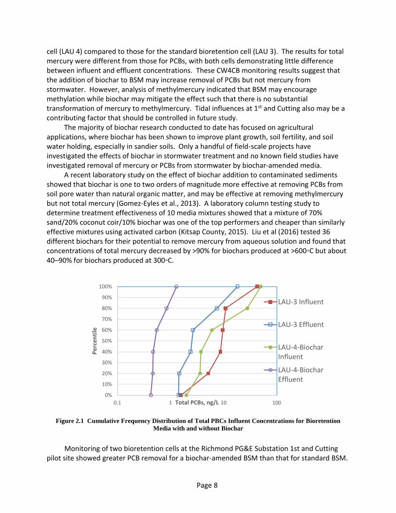
Page 8
cell (LAU 4) compared to those for the standard bioretention cell (LAU 3). The results for total mercury were different from those for PCBs, with both cells demonstrating little difference between influent and effluent concentrations. These CW4CB monitoring results suggest that the addition of biochar to BSM may increase removal of PCBs but not mercury from stormwater. However, analysis of methylmercury indicated that BSM may encourage methylation while biochar may mitigate the effect such that there is no substantial transformation of mercury to methylmercury. Tidal influences at 1st and Cutting also may be a contributing factor that should be controlled in future study.
The majority of biochar research conducted to date has focused on agricultural applications, where biochar has been shown to improve plant growth, soil fertility, and soil water holding, especially in sandier soils. Only a handful of field-scale projects have investigated the effects of biochar in stormwater treatment and no known field studies have investigated removal of mercury or PCBs from stormwater by biochar-amended media.
A recent laboratory study on the effect of biochar addition to contaminated sediments showed that biochar is one to two orders of magnitude more effective at removing PCBs from soil pore water than natural organic matter, and may be effective at removing methylmercury but not total mercury (Gomez-Eyles et al., 2013). A laboratory column testing study to determine treatment effectiveness of 10 media mixtures showed that a mixture of 70% sand/20% coconut coir/10% biochar was one of the top performers and cheaper than similarly effective mixtures using activated carbon (Kitsap County, 2015). Liu et al (2016) tested 36 different biochars for their potential to remove mercury from aqueous solution and found that concentrations of total mercury decreased by >90% for biochars produced at >600◦C but about 40–90% for biochars produced at 300◦C.
Figure 2.1 Cumulative Frequency Distribution of Total PBCs Influent Concentrations for Bioretention
Media with and without Biochar
Monitoring of two bioretention cells at the Richmond PG&E Substation 1st and Cutting pilot site showed greater PCB removal for a biochar-amended BSM than that for standard BSM.
0%
10%
20%
30%
40%
50%
60%
70%
80%
90%
100%
0.1 1 10 100
Pe
rce
nti
le
Total PCBs, ng/L
LAU-3 Influent
LAU-3 Effluent
LAU-4-BiocharInfluent
LAU-4-BiocharEffluent

Page 9
However, to date sampling has been limited to one test site and one biochar amendment, and the operational life of the amended media is unknown. Besides the CW4CB study, there are no published literature studies on field PCB and mercury removal for biochars. Additional field testing can confirm the effectiveness of bioretention implementation in more typical conditions, and laboratory testing is recommended as an initial screening to help identify potential biochars for field testing. Laboratory testing using actual stormwater from the Bay Area can be a cost-effective screening tool to identify biochar media that are effective for PCB removal, do not exacerbate mercury problems or even improve mercury removal, and meet operational requirements, including an initial maximum infiltration rate of 12 in/h and a minimum long-term infiltration capacity of 5 in/h.

Page 10
3. Study Goals
The goals of this study identified from the problem statements are as follows:
1. Quantify annual PCB and mercury load removals during maintenance (cleanout) of HDS units
2. Identify biochar media amendments that improve PCB and mercury load removal by bioretention BMPs
To reach these goals, the following management questions are prioritized as primary or secondary management questions.
3.1 Primary Management Questions
A properly conceived study will address the study goals in a manner that supports planning for future management actions or evaluating the effectiveness or impacts of existing management actions. The resulting primary management questions focus on performance and are:
1. What are the average annual PCB and mercury loads captured by existing HDS units in Bay Area urban watersheds?
2. Are there readily available biochar-amended BSM that provide significantly better PCB and mercury load reductions than standard BSM and meet MRP infiltration rate requirements?
The MRP infiltration rate requirements are described in Provision C.3.c of the MRP (SFBRWQCB, 2015). This provision states the following: “Biotreatment (or bioretention) systems shall be designed to have a surface area no smaller than what is required to accommodate a 5 inches/hour stormwater runoff surface loading rate, infiltrate runoff through biotreatment soil media at a minimum of 5 inches per hour, and maximize infiltration to the native soil during the life of the Regulated Project. In addition to the 5 inches/hour MRP requirement, for non-standard BSM the recently updated BASMAA specification requires “certification from an accredited geotechnical testing laboratory that the bioretention soil has an infiltration rate between 5 and 12 inches per hour” (BASMAA, 2016a).
3.2 Secondary Management Questions
Secondary management questions are helpful, but they are not critical to the usefulness of the study. Study scope, budget, and schedule constraints limit the extent to which they can be addressed. Possible secondary management questions include the following:
HDS 1. How does sizing of HDS units affect annual PCB and mercury loads captured in HDS
sediment? 2. Do design differences between HDS units (e.g., single vs multiple chambers) result in
significant differences in pollutant capture? 3. How does the frequency of cleanout of HDS units affect load capture?

Page 11
4. If present, does washout of HDS sediment depend on remaining sediment volume capacity?
5. Are there significant concentrations of PCBs in the pore (interstitial) water of HDS sediment?
6. Are PCBs and mercury removal correlated to removal of better-studied surrogate constituents, such as TSS?
7. Is there evidence of increased methylation within HDS sediment chambers?
Enhanced Bioretention 1. How does biochar performance vary with feedstock? 2. How does biochar performance vary with manufacturing method? 3. Should the biochar be mixed with the BSM or provided as a separate layer below the
standard BSM? 4. Does biochar have leaching issues or require conditioning before use? 5. How long does the improved performance of biochar-amended BSM last? 6. Does the promising media increase methylation of mercury? 7. What is the expected increase in BSM costs due to inclusion of media amendment? 8. Does knowledge of the association of PCBs and mercury to specific particle sizes
improve understanding of performance? 9. Is mass removal comparable to that expected from a conceptual understanding of
removal mechanisms?
The above secondary management questions are provided as examples, and the questions answered will depend on budget, schedule, and actual data collected.
3.3 Level of Confidence
The level of confidence in the answers to the above management questions depends on sample representativeness and size. Samples are considered representative if they are derived from sites or test conditions that are representative of the watershed or treatment being considered. A power analysis can be used after monitoring commences or at the end of a study to determine if sample size is sufficient to draw statistically valid conclusions at a pre-selected level of confidence. Power analysis can also be used prior to study commencement, but its usefulness in estimating sample size requirements may be limited by lack of knowledge of variability in the biochar-amended BSM data to be collected.
Level of confidence can also be assessed in terms of consistency of treatment (e.g., a particular biochar consistently shows better removals than other biochars for a variety of stormwaters), which can be assessed with non-parametric approaches such as a sign-rank test.
Data analysis approaches are discussed in Section 8.5.

Page 12
4. Study Design Options
An overview of the available study designs is presented here to understand the methods, value, and constraints of each design. This information is helpful in identifying which study designs are appropriate for the various management questions. To answer the primary management questions, the mass of pollutants captured must be quantified. This is accomplished by monitoring pollutant input and export for each HDS unit or media option, or directly quantifying captured pollutant. For example, the typical input and output pathways for a stormwater treatment measure (i.e., BMP) are illustrated in Error! Reference source not found.4.1. This overview describes how data are collected and how they are used to answer the primary study questions.
Filter Media
UnderdrainBMP
Outlet
Bypass
Aerial Deposition**
Catchment
Stormwater Input
Atmospheric
Losses**
BMP
*Assumed zero
** Assumed minor (usually unmeasured)
*** Lining, when present, helps prevent losses and gains from interaction with surrounding soils and water.
Vegetation
Removal*
Sediment
and Media
Removal*
Pollutant infiltration
into BMPInfiltration
into soil
Optional
Lining***
Figure 4.1 Typical BMP system and pollutant pathways
The study designs discussed here address major inputs and losses, but not all. Selection of study design is based on the management questions, the type of BMP(s), the study constraints, and the current and historic conditions of the study area. Each type of study has associated strengths and weaknesses as described below:
Influent-effluent monitoring Influent and effluent monitoring tests water going into and discharging from a selected BMP or treatment option for a particular storm event. This approach is typically used to assess BMP effectiveness. An advantage of this approach is its ability to discern differences in limited data sets. A weakness of this approach is that measured load reductions may not be representative of true load reductions if there is infiltration to the native soil, baseflow entering the BMP, or bypass flows that are not monitored
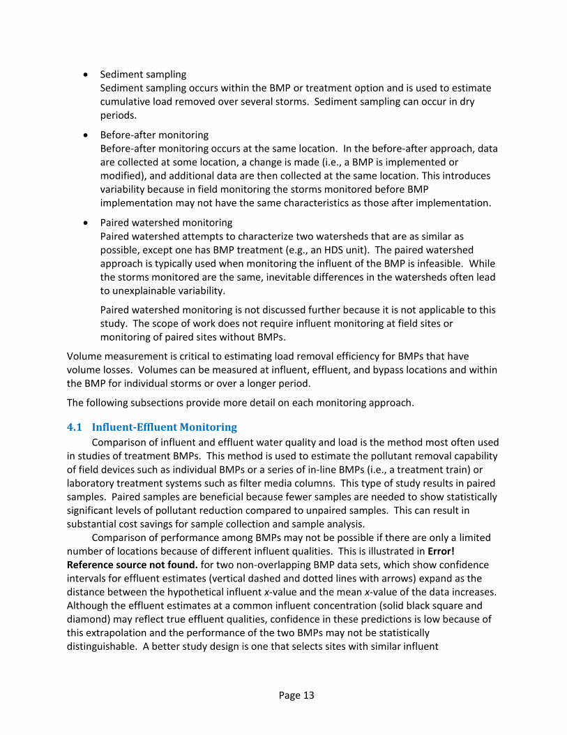
Page 13
Sediment sampling Sediment sampling occurs within the BMP or treatment option and is used to estimate cumulative load removed over several storms. Sediment sampling can occur in dry periods.
Before-after monitoring Before-after monitoring occurs at the same location. In the before-after approach, data are collected at some location, a change is made (i.e., a BMP is implemented or modified), and additional data are then collected at the same location. This introduces variability because in field monitoring the storms monitored before BMP implementation may not have the same characteristics as those after implementation.
Paired watershed monitoring Paired watershed attempts to characterize two watersheds that are as similar as possible, except one has BMP treatment (e.g., an HDS unit). The paired watershed approach is typically used when monitoring the influent of the BMP is infeasible. While the storms monitored are the same, inevitable differences in the watersheds often lead to unexplainable variability.
Paired watershed monitoring is not discussed further because it is not applicable to this study. The scope of work does not require influent monitoring at field sites or monitoring of paired sites without BMPs.
Volume measurement is critical to estimating load removal efficiency for BMPs that have volume losses. Volumes can be measured at influent, effluent, and bypass locations and within the BMP for individual storms or over a longer period.
The following subsections provide more detail on each monitoring approach.
4.1 Influent-Effluent Monitoring
Comparison of influent and effluent water quality and load is the method most often used in studies of treatment BMPs. This method is used to estimate the pollutant removal capability of field devices such as individual BMPs or a series of in-line BMPs (i.e., a treatment train) or laboratory treatment systems such as filter media columns. This type of study results in paired samples. Paired samples are beneficial because fewer samples are needed to show statistically significant levels of pollutant reduction compared to unpaired samples. This can result in substantial cost savings for sample collection and sample analysis.
Comparison of performance among BMPs may not be possible if there are only a limited number of locations because of different influent qualities. This is illustrated in Error! Reference source not found. for two non-overlapping BMP data sets, which show confidence intervals for effluent estimates (vertical dashed and dotted lines with arrows) expand as the distance between the hypothetical influent x-value and the mean x-value of the data increases. Although the effluent estimates at a common influent concentration (solid black square and diamond) may reflect true effluent qualities, confidence in these predictions is low because of this extrapolation and the performance of the two BMPs may not be statistically distinguishable. A better study design is one that selects sites with similar influent
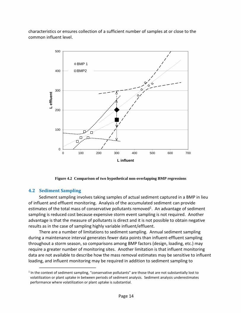
Page 14
characteristics or ensures collection of a sufficient number of samples at or close to the common influent level.
Figure 4.2 Comparison of two hypothetical non-overlapping BMP regressions
4.2 Sediment Sampling
Sediment sampling involves taking samples of actual sediment captured in a BMP in lieu of influent and effluent monitoring. Analysis of the accumulated sediment can provide estimates of the total mass of conservative pollutants removed1. An advantage of sediment sampling is reduced cost because expensive storm event sampling is not required. Another advantage is that the measure of pollutants is direct and it is not possible to obtain negative results as in the case of sampling highly variable influent/effluent.
There are a number of limitations to sediment sampling. Annual sediment sampling during a maintenance interval generates fewer data points than influent-effluent sampling throughout a storm season, so comparisons among BMP factors (design, loading, etc.) may require a greater number of monitoring sites. Another limitation is that influent monitoring data are not available to describe how the mass removal estimates may be sensitive to influent loading, and influent monitoring may be required in addition to sediment sampling to
1 In the context of sediment sampling, “conservative pollutants” are those that are not substantially lost to
volatilization or plant uptake in between periods of sediment analysis. Sediment analysis underestimates performance where volatilization or plant uptake is substantial.
0
100
200
300
400
500
0 100 200 300 400 500 600 700
L e
fflu
en
t
L influent
BMP 1
BMP2

Page 15
characterize pollutant loading. This limitation is addressed in this study during the data analysis by using model estimates of stormwater flows and pollutant loads from each HDS unit catchment to provide estimates of the influent and associated percent removals achieved.
Another limitation of sediment sampling is the potential error resulting in non-homogeneous pollutant distribution within the sediment. Compositing multiple samples will better characterize the sediment, much as the collection of several aliquots throughout a stormwater runoff event can better represent the total volume of water. Mixing the removed sediment before compositing can provide samples that are more homogeneous.
Consequently, the effectiveness of sediment sampling depends on the type of BMP. HDS are the best candidates for sediment sampling. The sumps are cleaned and empty at the start of the study, and the entire mass of retained sediment is removed at each maintenance event (sump cleanout). Conversely, bioretention has background sediment (planting media) that obscure pollutant accumulation. Since pollutants tend to accumulate on the surface of media (typically within the first few inches), surface sediments should be targeted when sampling these systems. Coring these systems and compositing the core sediments will most likely result in further dilution of the PCBs retained in the media, making quantification more difficult. For all systems, larger pieces of litter and vegetation may be difficult to include in the analysis. A conservative approach is to exclude larger material and assume these have little association with PCBs.
4.3 Before-After Monitoring
Pollutant removal can also be estimated by monitoring discharge quality for treatment devices before and after installation. This may be attractive for green street projects that have multiple BMPs with multiple influent and effluent locations. Monitoring all of these individual systems is almost impossible because of space constraints. Note that since the data from before/after implementation are unpaired, variability is expected to be larger and the number of samples required to show significant removal much higher than for paired samples.
Before-after monitoring is also applicable to laboratory test systems in which water quality is measured before and after a change is made. For example, the rate of adsorption or the adsorptive capacity of media can be determined by measuring the water quality before and after addition of a known quantity of media.

Page 16
5. Primary Data Objectives
The study design options discussed previously are matched to the primary management questions. The primary management questions require two data objectives: determine annual mass captured by HDS units and load removal by biochar-amended BSM. The primary management questions are:
1. What are the annual PCB and mercury loads captured by existing HDS units in Bay Area urban watersheds?
2. Are there readily available biochar-amended BSM that provide significantly better PCB and mercury load reductions than standard BSM and meet MRP infiltration rate requirements?
Monitoring to address the first management question should at minimum provide the average annual PCB and mercury loads captured by HDS units.
5.1 Data Objective 1: Annual Loads Captured by HDS Units
Determined by influent-effluent monitoring for individual storm events over one or more seasons or filter media/sediment sampling at end of each season.
Options: Influent-effluent monitoring. Requires monitoring of as many storms as possible over a
season and flow measurement in addition to water quality sampling. Flow measurement is a critical component for estimating stormwater volumes treated, retained, and bypassed, and is often associated with additional measurements such as water depth within a BMP to estimate bypass and retention.
Filter media/sediment sampling. Requires sampling at end of season but does not require influent/effluent water quality or flow measurement. Sediment sampling has a high value for estimating annual mass removal because a single composite sample of retained sediment over a season can yield an estimate of load removal for the constituents analyzed. However, influent characterization would also help explain mass removal performance. This method is most appropriate when applied to HDS systems because they can isolate retained sediment.
5.2 Data Objective 2: Loads Reduced by Biochar-Amended BSM
Determined by influent-effluent monitoring or filter media/sediment sampling for individual events until sufficient data are available for statistical analysis.
Options: Influent-effluent monitoring. Requires monitoring of multiple individual events and flow
measurement in addition to water quality sampling. Accurate flow measurement in BMPs is difficult because flows can vary an order of magnitude during individual events and measurements may be required at multiple locations within a device because of bypass, infiltration etc. (see Figure 4.2). This complexity introduces a great degree of variability in the monitored data that can substantially increase the number of data points required to show statistically significant load removals, particularly for BMPs such as HDS units that

Page 17
show relatively small differences between influent and effluent load reductions. This option is most appropriate for testing filter media, for example in laboratory experiments, in which accurate flow measurements are possible and sampling of accumulated sediment is infeasible.
Filter media/sediment sampling. Requires sampling after individual events but does not require influent/effluent water quality or flow measurement. This method is not feasible for filter media because the retained sediment cannot be isolated from the filter media.
Page 18
6. BMP Processes and Key Study
Variables
The treatment mechanisms that occur in a BMP help inform selection and control of the study variables. These treatment mechanisms, also called unit processes, may include physical, chemical, or biological processes. The primary physical, chemical, and biological processes that are responsible for removing contaminants include the following:
Sedimentation – The physical process by which suspended solids and other particulate matter are removed by gravity settling. Sedimentation is highly sensitive to many factors, including size of BMP, flow rate/regime, particle size, and particle concentration, and it does not remove dissolved contaminants. Treated water quality is less consistent compared to other mechanisms due to high dependence on flow regime, particle characteristics, and scour potential.
Flocculation – Flocculation is a process by which colloidal size particles come out of suspension in the form of larger flocs either spontaneously or due to the addition of a flocculating agent. The process of sedimentation can physically remove flocculated particles.
Filtration – The physical process by which suspended solids and other particulate matter are removed from water by passage through layers of porous media. Filtration provides physical screening of particles and trapping of particles within the porous media. Filtration depends on a number of factors, including hydraulic loading and head, media type and physical properties (composition, media depth, grain size, permeability), and water quality (proportion of dissolved contaminants, particle size, particle size distribution). Compared to sedimentation, filtration provides a more consistent treated quality over a wider range of contaminant concentrations.
Infiltration – The physical process by which water percolates into underlying soils. Infiltration is similar to filtration except it results in overall volume reduction.
Screening – The physical process by which suspended solids and other particulate matter are removed by means of a screen. Unlike filtration, screening is used to occlude and remove relatively larger particles and provide little or no removal for particles smaller than the screen opening size and for dissolved contaminants.
Sorption – The processes of absorption and adsorption occur when water enters a permeable material and contaminants are brought into contact with the surfaces of substrate media, plant roots, and sediments, resulting in short-term retention or long-term immobilization of contaminants. The effectiveness of sorptive processes depends on many factors, including the properties of the water (contaminant concentration, particle concentration, organic matter, proportion of dissolved contaminants, particle size, pH, particle size and charge), media type (surface charge, absorptive capacity), and contact time.

Page 19
Chemical Precipitation – The conversion of contaminants in the influent stream, through contact with the substrate or root zone, to an insoluble solid form that settles out. Consistent performance often depends on controlling other parameters such as pH.
Aerobic/Anaerobic Biodegradation – The metabolic processes of microorganisms, which play a significant role in removing organic compounds and nitrogen in filters.
Phytoremediation – The uptake, accumulation, and transpiration of organic and inorganic contaminants, especially nutrients, by plants.
The relative importance of individual treatment mechanisms depend to a large extent on the chemical and physical properties of the contaminant(s) to be removed i.e. the influent quality. The two contaminants of interest in this study are PCBs and mercury. PCBs are relatively inert hydrophobic compounds that have very limited solubility and a strong affinity for organic matter. They are often associated with fine and medium-grained particles in stormwater runoff, making them subject to removal through gravitational settling or filtering through sand, soils, media or vegetation. Most of the mercury in water, soil, and sediments is in the form of inorganic mercury salts and organic forms of mercury such as methylmercury that are strongly adsorbed to organic matter (e.g., humic materials). In general, mercury is most strongly associated with fine particles while PCBs are generally associated with relatively larger and/or heavier particles. It is therefore expected that sedimentation, flocculation, and related processes will be less effective for mercury removal than for removal of PCBs (Yee and McKee, 2010).
The following subsections provide a brief description of the BMP types being evaluated in this study, the unit processes involved in each, and key variables that indicate possible data collection approaches. The final selection of the quantity and type of data to collect is presented in the “Optimized Study Design” section.
6.1 HDS Units
Hydrodynamic separators rely on sedimentation and screening as the primary removal mechanism for sediment and particulate pollutants. Treatment performance is highly dependent on the following:
- Influent quality (contaminant concentration, proportion of dissolved contaminants, particle size, particle size distribution, and particle density)
- BMP design and hydraulic loading/flow regime (size of unit versus catchment area) - Operational factors (remaining sediment capacity)
HDS effluent quality is highly variable, particularly for contaminants such as mercury that are associated with fine particles that are not as effectively removed in HDS. These devices are expected to require a relatively large number of influent-effluent samples to demonstrate statistically significant reductions in pollutant concentrations. Therefore, analysis of retained sediment is an appropriate alternative to influent-effluent sampling for determining pollutant mass captured. Sediment can be analyzed when the device is cleaned.
Page 20
6.2 Bioretention
Bioretention is a slow-rate filter bed system. It is planted with macrophytes (typically shrubs and smaller non-woody vegetation). The major sediment removal mechanism is physical filtration through the planting media. When retention time is sufficient, dissolved constituents can be removed by sorption to plant roots in the planting media, which typically contains clays and organics to enhance sorption. Treatment performance is highly dependent on the following variables:
- Influent quality (contaminant concentration, particle concentration, organic matter, proportion of dissolved contaminants, particle size, particle size distribution)
- BMP design and hydraulic loading rate/head (size of the unit in relation to catchment area and storm character)
- Media type and properties (composition, grain size, grain size distribution, adsorptive properties, and hydraulic conductivity)
- Volume reduction by infiltration - Operational factors (surface clogging, short-circuiting)
The effluent quality from bioretention and enhanced bioretention is expected to be consistently higher than for sedimentation-type BMPs. These devices are expected to require a relatively fewer number of samples than HDS units to demonstrate statistically significant reduction because of better treatment of fine particles and dissolved contaminants.
It is important to note that laboratory and not field bioretention systems are of interest in this study. These laboratory systems, essentially cylindrical columns filled with the media being tested, attempt to simulate most, but not all, of the chemical, biological, and physical processes that occur in field devices. For example, volume reductions due to infiltration are not simulated in laboratory column experiments. The advantages of using media columns as proxies for field devices include improved control over operation, monitoring, and sample collection in ways that would be impractical in the field. This improved control makes it possible to test a large number of potential media and identify the most promising for future field testing.

Page 21
7. Monitoring and Sampling
Options
Key variables that affect water quality and sediment quality data are identified from knowledge of treatment processes. The following lists the process variables identified through knowledge of the treatment processes:
- Influent quality (contaminant concentration, particle concentration, organic matter, proportion of dissolved contaminants, particle size, particle size distribution, particle density)
- BMP design and hydraulic loading (flow rate, hydraulic head, flow regime) - Media type and properties (composition, grain size, grain size distribution, adsorptive
properties, and hydraulic conductivity) - Operational factors (surface clogging, short-circuiting, remaining sediment capacity)
Some of the above variables can be controlled and others are measured to determine their effect on water quality and sediment quality. Inevitably, some variables will be beyond the control of the study but their expected impact should be considered based on theory, past experience, models, or observations from other studies.
7.1 HDS Units
7.1.1 Influent Quality
The location of the BMP can greatly affect influent water quality such as pollutant concentrations and particle characteristics because land use and land cover affect sediment mobilization and pollutant concentrations within the sediments. Land use is often used as an indicator of pollutant loading. The land uses of the areas of interest include industrial, commercial/mixed use, roads/rail, institutional, and residential. Because of past use of PCB and past PCB and mercury handling practices, age of the land use is also important, with generally higher concentrations from older industrial, commercial, and transportation areas, and lower concentrations from newer residential areas. However, PCB analysis by the San Francisco Estuary Institute (SFEI) showed that PCB concentration patterns were patchy within larger urban watersheds with higher concentrations. This finding indicates that mass reductions of PCBs may require site-specific sampling of influent loads or site-specific quantification of mass removed. Mercury data suggest areas with higher mercury concentrations are not as pronounced although generally where there is PCB contamination there is also high to moderate Hg contamination (Yee and McKee, 2010).
Since HDSs are primarily installed for trash capture, their distribution within the study area is assumed to be random. However, the primary interest is in watersheds with relatively high pollutant loads that are most likely to result in significant removal in HDSs (e.g., the Leo Avenue watershed). Land use or land use based pollutant yields can be used to represent average influent water quality when influent monitoring is not conducted.
Page 22
Figure 7.1 shows the land use based PCB and mercury loadings for key designated land use types. It can be seen that unit PCB loading from watersheds with higher PCB concentrations and mercury loading from old industrial watersheds are substantially higher than the other land uses. Assuming particle size, particle size distribution, and other stormwater characteristics are similar for the different land uses, HDSs in higher concentration watersheds or old industrial watersheds are expected to capture much higher pollutant loads than those in other watersheds.
Figure 7.1 Land Use based PCB and Mercury Loading based on BASMAA Integrated Monitoring Reports
(SFEI, 2015)
A preliminary land use based study design could categorize HDS sites as show in Table 7.1.
Table 7.1 HDS Sampling Design based on Watershed Land Use
Land Use HDS Samples
Higher Concentration X, X, X1
Old Industrial X, X, X1
Old Urban X, X, X1
1 – “X” represents a sample from a selected HDS unit in the specified land use category.

Page 23
The above design is appropriate if HDS units can be categorized easily into one of the three land use categories. A review of the land uses within HDS watersheds indicates that most HDS units are in predominantly old urban watersheds, and it is unclear how many HDSs are within areas with higher PCB concentrations (Table 7.2).
Table 7.2 Percent of Land Use in HDS Watershed Areas (Based on FY 2015-16 Co-permittee Annual Reports, Section 10 - Trash Load Reduction. Source: Chris Sommers Personal Communication)
Given the few sites in categories other than old urban, an alternative study design based on mixed land uses may be more appropriate (Table 7.3).
HDS Catchment ID New Urban Old Industrial Old Urban Open Space Other
287; Sonora Ave 16 84 1
27A 15 50 34 2
996; Parkmoor Ave 1 98 1
1084; Oswego 0 89 0 10
600; Edwards Ave 33 39 28
611; Balfour 14 55 30
1082; Melody/33rd 0 97 3
612; Lewis 93 7
604; Sunset 96 4
1012; Blossom Hill/Shadowcrest 100 0
1083; Lucretia 0 98 1 1
1002; Selma Olinder 10 86 5
995; Dupont St. 9 91 0
9-A; 73rd Ave and International Blvd 0 94 6
475; 7th 68 29 3
509; Coyote 22 77 1
47 99 1
8-A; Alameda Ave near Fruitvale 40 57 4
575; Bulldog 6 93 1
601; W. Virginia 7 90 3
1504; Phelps 100 0
390; Remillard 4 87 10
Tennyson at Ward Creek 1 97 2
W Meadow Dr 2 97 1
Leland and Fair Oaks 1 99
Ward and Edith 100 0
5-D; 22nd and Valley 1 99 0
8-C; High St @ Alameda Bridge 67 32 0
5-G; Perkins & Bellvue (Nature Center) 100
999; William 0 95 5
Main St and Hwy 1 85 15
Central Expy at Fair Oaks 11 89 0
393; Wool Creek 18 78 4
5-C; 27 St & Valdez Ave 2 98
998; Pierce 1 96 3
Maple and Ebensburg 98 2
Ventura Ave 99 1
Golden Gate and St Patrick 100 0
5-A; Euclid Ave @ Grand Ave 100
5-H; Lake Merritt (SD Outfall 11) 100
5-B; Staten Ave & Bellvue 100
Central Expy at De la Cruz 33 67
5-I; Lake Merritt (SD Outfall 26) 100
Mathilda overpass project CDS2 0 100
Mathilda overpass project CDS1 10 84 7

Page 24
Table 7.3 HDS Sampling Design based on Predominant Land Use
Predominant Land Use HDS Samples
Higher Concentration/Old Industrial X, X, X1
Old Urban/Old Industrial X, X, X1
New Urban/Old Urban X, X, X1
1 – “X” represents a sample from a selected HDS unit in the specified land use category.
The sampling design in Table 7.3 assumes that at least three HDS units are available for sampling in each PCB land use category. The sampling design may need to be modified further if there are an insufficient number of units available for sampling. For example, any site with more than 30% old industrial may be considered especially if it is a mixed zoned watershed (with industrial, commercial, residential and transportation land uses). The range of values in each land use category can be determined upon review of the most recent information. The design in Table 7.3 assumes that the characteristics of the runoff (e.g., particle sizes) are similar for the different land uses and only the yield is different.
Only sediment sampling is proposed for HDS. Since HDS influent-effluent monitoring is not required, variables such as proportion of dissolved contaminants, particle size, particle size distribution, and particle density are not measured or controlled, but their effect on influent quality and treatment is accounted for by randomly selecting HDSs within each land use category.
7.1.2 BMP Design and Hydraulic Loading
BMP design and hydraulic loading, which depends on the size of the BMP, can have a substantial impact on effluent water quality and the quantity of sediment retained in a BMP. Consequently, a full range of BMP designs and sizes are of interest. Properly sized, BMPs infrequently exceed their design capacity. However, BMPs are not always sized to standard specification, especially in retrofit environments in which typical hydraulic loading is much higher due to space constraints.
HDS units are typically proprietary and designs and sizing vary widely. Sediment capture may vary because of design differences such as number of chambers and design of overflow weirs and baffles, as well as different sizing criteria that can greatly affect both hydraulic loading and flow regime. The purpose of the study is to characterize sediment in HDS units in the study area. Since BMP design and sizing are important factors affecting HDS performance, it is necessary to include a range of HDS units in the study design and not just randomly select HDS units. A randomized blocked study design is therefore considered more appropriate than a completely random one that may result in an insufficient number of HDS units of a certain size.
In a randomized design, one factor or variable is of primary interest (e.g., land use), but there are one or more other confounding variables that may affect the measured result but are not of primary interest (e.g., HDS design, HDS size). Blocking is used to remove the effects of one or more of the most important confounding variables and randomization within blocks is then used to reduce the effects of the remaining confounding variables. An appropriate sampling design could therefore be land use as the primary factor and HDS size as the blocking factor. Since the population of HDS units in the land use categories of interest is limited, only

Page 25
two size blocks are used (≤ 50th percentile, > 50th percentile), and other variables such as design differences are accounted for by random selection within each block (Table 7.4).
Table 7.4 HDS Sampling Design based on Predominant Land Use and HDS Size
Predominant Land Use HDS Size
≤50th percentile >50th percentile
Higher Concentration/Old Industrial X, X, X1 X, X, X1
Old Urban/Old Industrial X, X, X1 X, X, X1
New Urban/Old Urban X, X, X1 X, X, X1
1 – “X” represents a sample from a selected HDS unit in the specified land use category.
For the sampling design in Table 7.4, an HDS size factor is required to differentiate the two types of sizes that are of interest. In controlled field study of 4 different proprietary HDS units and laboratory testing of 2 other units, Wilson et al. (2009) developed a performance function (treatment factor) that reasonably predicted the removal efficiency of a given hydrodynamic separator. The performance function explained particle removal efficiency in terms of a Péclet number, Pe, which accounts for particle settling and turbulent diffusion. In the following equation, Vs is the particle settling velocity, h is the settling depth in the device, d is the device diameter, and Q is the flow through the device:
𝑃𝑒 =𝑉𝑠ℎ𝑑
𝑄
The above Péclet number (Wilson et al’s performance function) can be used in the sampling design as the HDS size factor. For grouping the available HDS units into the two blocks, information is required on the particle diameter and design parameters for each device (settling depth, diameter, and design flow). Particle diameter can be assumed to be 75 µm, which is the critical size used for partitioning PCB fractions in Yee and McKee (2010), and is also approximately the size separating silt and fine sand size particles. The design flow can be calculated from knowledge of the drainage area to the device and a standard design storm. Note that the design flow should not be based on manufacturer guidance because different manufacturers use different sizing criteria and device sizing may not always follow manufacturer guidance.
The final sampling design may need revision depending on the monitoring approach, availability of HDSs, information on watershed land use and sizing, and the level of participation from municipalities.

Page 26
7.1.3 Operation and Maintenance
Maintenance frequency can greatly impact BMP performance. For sedimentation BMPs such as HDS, sediment levels may exceed the sediment capacity of the BMP, decreasing the volume for sedimentation and increasing scour.
Operation and maintenance (e.g., cleanout frequency) are not of direct interest in this study and their effect on treatment is not being tested. However, these are confounding variables that need to be excluded. In the HDS sediment sampling design, HDS units that are considered at capacity or will reach capacity during the study should be excluded from the population of interest. Field observations are required to make this determination (e.g., whether the screen is blocked). These units can be cleaned out and sampled in a subsequent year. For each selected HDS unit, maintenance schedules (past and current) will need to be reviewed to determine the time period over which sediment accumulated.
7.2 Enhanced Bioretention
7.2.1 Influent Quality
The purpose of the laboratory testing is to screen alternative biochar-amended BSM and identify the most promising for further field testing. The laboratory testing requires influent-effluent monitoring. Influent water characteristics can vary depending on the source of the test water. PCB and mercury loading is largely a result of historic activities that result in accumulation in sediments of pervious areas. Mobilization of these sediments may require exceeding site-specific intensity and volume thresholds. Storm intensity is critical to detach and mobilize particles and storm volume must exceed any depression storage within the pervious areas. However, the precise effect of storm intensity and volume on the mobilization of PCB-contaminated and mercury-contaminated sediments has not been established. Influent water characteristics also depend greatly on drainage area characteristics including traffic and industrial and commercial activity.
Since the purpose of the laboratory study is to screen alternative biochar-amended BSM that can be used throughout the Bay Area, collection and use of stormwater from one or more representative watersheds is preferred. A preliminary review of available Bay Area stormwater runoff monitoring data from 27 sites (Table 7 of SFEI 2015) suggests median PCB concentration is about 9 ng/L. Therefore, one or more previously monitored watersheds with mean PCB concentrations well above 10 ng/L may be appropriate for collection of stormwater for the laboratory testing. Since the relative treatment performance of the various media at even lower concentrations may be different, additional tests with diluted stormwater may be required to confirm study results.
Storms from the representative watershed should be targeted randomly without bias, thereby accounting for the effects of storm intensity and ensuring variability in contaminant concentration, proportion of dissolved contaminants, particle size, particle size distribution, and particle density. To achieve this, minimal mobilization criteria should be used to ensure predicted storm intensity and runoff volume are likely to yield the desired volume.
Page 27
7.2.2 BMP Design and Hydraulic Loading
The design variables in the enhanced bioretention testing laboratory study include media type, media depth, and media configuration. Media type is a key variable that is discussed further below. Testing the effect of different media depths or media configurations is not a research objective of the laboratory study, so these can be fixed for all experiments. Typical bioretention media depth in the Bay Area is 18 inches, so all column experiments should use 18 inches of BSM. In the Richmond PG&E Substation 1st and Cutting enhanced BSM testing, the biochar was not installed as a separate layer but was instead mixed with the standard BSM. It is unclear how treatment is affected by these two media configurations, but for consistency with previous field work the biochar and standard BSM should be mixed.
Hydraulic loading is a controlled variable that can be kept constant for all columns. Since the laboratory study is attempting to replicate field bioretention, the hydraulic loading can be the design loading for bioretention. Bioretention designs in the Bay Area typically have a maximum ponding depth of 6 inches, so a loading of 6 inches could be used for the column tests. There are two options for loading the columns: pump and manual. Peristaltic pumps are ideal for controlled loading, but in this study manual loading (batch loading) is more appropriate because of the potential for PCBs and mercury to stick to tubing, pump parts, etc. For manual loading, up to 10 inches of stormwater may be needed each time to ensure sufficient sample volume.
7.2.3 Media Type and Properties
Media type and properties have a substantial effect on the treatment performance of filtration devices. This group of variables include composition, grain size, grain size distribution, adsorptive properties such as surface area, and hydraulic conductivity. Media composition is a primary variable that accounts for differences in the biochars used and the proportion of each biochar in the amended BSM mix. The other variables (grain size, grain size distribution, adsorptive properties, and hydraulic conductivity) are not of direct interest in this study and are assumed to vary randomly or are controlled through screening experiments that limit their variability.
Biochar is produced from nearly any biomass feedstock, such as crop residues (both field residues and processing residues such as nut shells, fruit pits, and bagasse); yard, food, and forestry wastes; animal manures, and solid waste. Biochar feedstock and production conditions can vary widely and significantly affect biochar properties and performance in different applications, making it difficult to compare performance results from one study to another (BASMAA, 2017a). A laboratory study that characterized the physical properties of six different waste wood derived biochars found particle sizes ranging from over 20mm to fine powder and surface areas ranging from 0.095 to 155.1 m2/g (Yargicoglu et al., 2015). The variability in biochar types and properties is expected to result in large variation in treatment efficiency and infiltration rates. Given the large number of potential biochars that could be tested and the need to meet an initial maximum 12 in/h infiltration rate and a minimum long-term infiltration rate of 5 in/h, a phased study design is appropriate. In such a phased study, promising readily available biochars are first identified through a review of the literature, and hydraulic screening experiments are performed on biochar-BSM media mixes to ensure infiltration rates are met

Page 28
prior to performance testing. This approach is expected to be the most cost-effective because it reduces analytical costs.
There is little information on hydraulic properties of bioretention media amended with biochar, and it is not clear what percentage of the amended BSM should be biochar to maximize treatment benefit. Given the variable physical size of the biochar media, relatively fine biochars could result in a mix that does not meet the initial 12 in/h maximum infiltration rate or minimum 5 in/h long-term infiltration rate. Kitsap County (2015) tested a BSM mix containing 60% sand, 15% Compost, 15% Biochar, and 10% shredded bark, and found that the biochar mix had an infiltration rate of only 6.0 in/h. One conclusion of the study was that the reduction in infiltration rate with the biochar additive was most likely because of fines in the biochar. To overcome this, hydraulic screening experiments are required in which the infiltration rate for each media mix is measured prior to water quality testing to ensure that both the maximum and minimum rates are met. Initially, each biochar can be mixed with standard BSM at a rate of 25% biochar by volume (the same as that at the CW4CB Richmond PG&E Substation 1st and Cutting site). Hydraulic conductivity can be determined using the method stated in the BASMAA soil specification, method ASTM D2434, which requires measurement of water levels and drain times. If a mix does not meet the infiltration requirements, the percentage of biochar is adjusted and the new mix tested. Amended mixes that do not meet the infiltration rate requirements are removed from further consideration (i.e. the effect of hydraulic conductivity is controlled by screening).
The final phase of the laboratory study can be column testing to identify the most effective amended BSM mixes for field testing. An influent-effluent monitoring design is typically used in column testing and media effectiveness is assessed on a storm-to-storm basis with real stormwater collected in the Bay Area. Only media mixes that have passed the hydraulic screening should be tested. All media columns should be sufficiently large or replicated to account for or minimize the impact of variability in media installation and experimental technique. Standard BSM should be used as a control since the primary interest is to identify media mixes that perform significantly better than standard BSM. An example of the column sampling design for 5 new media mixes and one standard BSM control is shown in Table 7.5. The key variable of interest in the sampling design in Table 7.5 is the media mix (composition).
Table 7.5 Example Sampling Design for Laboratory Column Experiments
Biochar/BSM Mix Column Samples
A Mix X, X, X1
B Mix X, X, X1
C Mix X, X, X1
D Mix X, X, X1
E Mix X, X, X1
Control Mix X, X, X1
1 – “X” represents an influent or effluent sample.

Page 29
7.2.4 Operation and Maintenance Parameters
Operational life depends on the capacity to pass the minimum required stormwater flows. Like media life, operational life is important because it determines the frequency and cost of maintenance requirements. Maintenance frequency can greatly impact BMP performance, and lack of maintenance can lead to surface clogging and sediment clogging in the inlets which reduces treatment capacity and increases bypass and overflow. Operation and maintenance are not of direct interest in this study and their effect on treatment is not being tested. However, these are confounding variables that need to be excluded.
Media mixes that do not meet the maximum 12 in/h and minimum 5 in/h infiltration rates can be excluded by hydraulic screening experiments (discussed above). As well as meeting the maximum 12 in/h initial infiltration rate requirement, these screening experiments help ensure that the BSM mixes do not fail during the laboratory testing. However, operational performance in laboratory experiments is not expected to be representative of that in the field because of differences in influent quality, variability in loading, effects of vegetation, etc. Therefore, laboratory estimates of long term infiltration rate are of little use and field testing is required to confirm that selected media mixes meet the long-term minimum infiltration rate of 5 in/h. The laboratory testing, however, can provide relative comparisons of hydraulic performance that can be used to decide and screen out media mixes that are likely to hydraulically fail in the field.
7.3 Uncontrolled Variables and Study Assumptions
The following assumptions were adapted from the Caltrans PSGM (Caltrans, 2009):
Site Assumptions HDS sediment concentrations are representative of the land use within the
watershed, i.e. there are no sources of sediment from adjoining watersheds, from illicit discharges, or from construction activities
HDS sediment or influent is not affected by base flow, groundwater, or saltwater intrusion
Differences in storm patterns throughout the Bay Area are not sufficient to change the HDS performance measurements
Water quality of stormwater collected for laboratory testing is representative of that observed in Bay Area urban watersheds
BMP Operation Assumptions Sampled HDS units operated as designed (e.g., no significant scouring) Volatilization of pollutants is negligible There is no short-circuiting of flows in laboratory column studies
Media Selection Assumptions The readily available biochars selected are representative of all biochars Selected media do not leach contaminates and media conditioning (e.g.,
washing) is not required
Monitoring Assumptions

Page 30
Data collected from a few sites over a relatively short time span will accurately represent sediment at all HDS sites over longer time frames
There are minimal contaminant losses in collecting and transporting water for laboratory experiments
Water quality of stormwater for laboratory tests does not change significantly during each test
Stormwater loading of laboratory columns is representative of loading in the field
Long-term infiltration performance of biochar mixes is to be tested in the field
Page 31
8. Final Study Design
The study design is optimized to answer the primary management questions within the available budget. The design used prioritizes sampling of HDS units, but allocates sufficient funding for minimum sampling requirements for the laboratory media testing study. Monitoring that does not relate directly to the primary management questions is considered lower priority.
8.1 Statistical Testing & Sample Size
In a traditional test of a treatment, the null hypothesis is that there is no difference between the influent and effluent of a treatment (i.e., the treatment does not work). In the case of HDS sampling, influent-effluent sampling is not required, and interest is only in determining if HDS units remove PCBs and mercury and how the sediment concentrations and load removals vary for different land uses, and for different rainfall and stormwater flow characteristics. Statistical testing in the HDS study is therefore limited to testing if there is a difference in the concentrations and loads captured by HDS units in different watersheds. This testing will require sampling of a sufficient number of HDS units in each land use category associated with differing pollutant load yields.
In the laboratory study, influent-effluent sampling is required and traditional statistical tests can be used depending on sample size.
As well as traditional statistical testing, confidence in the conclusions can be established by comparing total PCB and mercury performance to that for other constituents that directly affect it (e.g., suspended solids, total organic carbon) or have similar chemistry (e.g., other organics). As stated previously, total PCB and mercury concentrations are expected to correlate to some extent with particulates and organics. Comparisons to other constituents are particularly useful for studies in which treatment is expected to be low and the corresponding sample size requirements very high.
Sample size requirements are smaller for paired sampling designs (i.e., influent and effluent sampling for the same storm event) than for independent sampling designs. Paired sampling is not possible for the HDS sampling study that has no influent-effluent monitoring, but is possible in the laboratory media testing study. Additionally, the number of samples required to show significant treatment are generally fewer for filtration-type BMPs than sedimentation-type BMPs because of their better and more consistent treatment.
8.2 Constituents for Sediment Analysis
Constituents selected for HDS sediment analysis must meet the data objectives discussed previously in “Primary Data Objectives”, and be consistent with Table 8.3 of the MRP (SFRWQCB, 2015). Sediment samples will be screened using a 2 mm screen prior to analysis. Table 8.1 lists the constituents for sediment quality analysis. Total organic carbon (TOC) is included because it is a MRP requirement and can be useful for normalizing PCBs data collected for the sediment.
The primary objective of sediment analysis is quantification of the mass of PCBs and mercury accumulating within HDS units. Consequently, PCBs and total mercury are analyzed
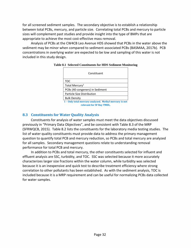
Page 32
for all screened sediment samples. The secondary objective is to establish a relationship between total PCBs, mercury, and particle size. Correlating total PCBs and mercury to particle sizes will complement past studies and provide insight into the type of BMPs that are appropriate to achieve the most cost-effective mass removal.
Analysis of PCBs at the CW4CB Leo Avenue HDS showed that PCBs in the water above the sediment may be minor when compared to sediment-associated PCBs (BASMAA, 2017b). PCB concentrations in overlying water are expected to be low and sampling of this water is not included in this study design.
Table 8.1 Selected Constituents for HDS Sediment Monitoring
Constituent
TOC
Total Mercury1
PCBs (40 congeners) in Sediment
Particle Size Distribution
Bulk Density 1 – Only total mercury analyzed. Methyl mercury is not
relevant for SF Bay TMDL.
8.3 Constituents for Water Quality Analysis
Constituents for analysis of water samples must meet the data objectives discussed previously in “Primary Data Objectives”, and be consistent with Table 8.3 of the MRP (SFRWQCB, 2015). Table 8.2 lists the constituents for the laboratory media testing studies. The list of water quality constituents must provide data to address the primary management question to quantify total PCB and mercury reduction, so PCBs and total mercury are analyzed for all samples. Secondary management questions relate to understanding removal performance for total PCB and mercury.
In addition to PCBs and total mercury, the other constituents selected for influent and effluent analysis are SSC, turbidity, and TOC. SSC was selected because it more accurately characterizes larger size fractions within the water column, while turbidity was selected because it is an inexpensive and quick test to describe treatment efficiency where strong correlation to other pollutants has been established. As with the sediment analysis, TOC is included because it is a MRP requirement and can be useful for normalizing PCBs data collected for water samples.

Page 33
Table 8.2 Selected Aqueous Constituents for Media Testing in Laboratory Columns
Constituent
SSC
Turbidity
TOC
Total Mercury1
PCBs (40 congeners) in Water 1 – Only total mercury analyzed. Methyl mercury is not
relevant for SF Bay TMDL.
8.4 Budget and Schedule
The monitoring budget for the study is approximately $200,000. A contingency of 10 percent of the water quality monitoring budget is recommended to account for unforeseen costs such as equipment failure. Another constraint is that all sampling will occur in one wet season.
8.5 Optimized Study Design
The optimized study designs are presented in Tables 8.3 and 8.4 for the HDS Monitoring and Enhanced Bioretention studies, respectively. Several iterations were analyzed and the study designs shown are based on best professional judgment to allocate the budget to the various data collection options.
The final design for the HDS monitoring study is based on selection and sampling of 9 HDS units in key land use areas. The number of units that can be sampled is limited because sampling is expected to be opportunistic as part of regular maintenance programs. Therefore, a simple design with 9 units is appropriate. The data analysis will evaluate the percent removal achieved for each HDS unit during the time period of interest (i.e., the time period between the date of the previous cleanout, and the current cleanout date for each HDS unit sampled) by incorporating modeled estimates of stormwater volumes and associated pollutant loads for each HDS unit catchment. Because HDS units are sized to treat stormwater runoff from storms of a given size and intensity, excess flows for storms exceeding the design capacity will bypass the unit and are not treated. Storm by storm analysis of rainfall data during the time period of interest will allow estimation of the total stormwater volume and pollutant load to the catchment during each storm, as well as the volume and pollutant load that bypassed the HDS unit and was not treated. This information will then be combined with the measured pollutant mass captured by each HDS unit to quantify the percent removal of PCBs and mercury from the total catchment flow, and the percent removal of PCBs and mercury from the treated flow. For each HDS unit sampled in the study, the total and treated pollutant mass removed will be calculated using the following equations.
(1) Total Pollutant Mass Removed (%) = [MHDS-i/MCatchment-i] x 100%
(2) Treated Pollutant Mass Removed (%) = [MHDS-i/(MCatchment-i- MB)] x 100%

Page 34
Where:
MHDS-i the total POC mass captured in the sump of HDS Unit i over the time
period of interest
MCatchment-i the total POC mass discharged from Catchment-A (the catchment
draining to HDS unit A) over the time period of interest
MB the total POC mass that bypassed HDS unit A over the time period of
interest The following inputs will be measured or modeled for the time period of interest for use
in the equations above:
Total PCBs and mercury mass captured by a given HDS unit. This is the mass measured in
each HDS unit during this project.
The total stormwater volume and associated PCBs and mercury load from the HDS unit
catchment. This will be modeled on a storm by storm basis using available rainfall data,
catchment runoff coefficients, and assumed pollutant stormwater concentrations.
The stormwater volume and associated PCBs and mercury load that bypassed the HDS
unit. The bypass volume (and associated pollutant load) during each storm (if any) will
be calculated based on the design criteria for a given HDS unit.
The total PCBs and mercury load treated by a given HDS unit. This will be determined by
subtracting the bypass load (if any) from the total pollutant load for the catchment.
The corresponding design for the enhanced BSM study is based on testing of readily
available biochars in hydraulic screening experiments followed by column testing of up to five promising BSM mixes as well as a standard BSM control mix. The final number of BSM mixes will depend on availability and media properties (e.g., expected hydraulic conductivity). The optimized designs will yield 33 data points for the key data objectives, 9 from the HDS monitoring study and 24 from the enhanced BSM media testing column study.

Page 35
Table 8.3 HDS Monitoring Study Design
Primary Management Question(s)
What are the annual PCB and mercury loads captured by existing HDS units in Bay Area urban watersheds and the associated percent removal?
Type of Study Sediment monitoring; modeling stormwater volume and pollutant load
Data Objective(s) Annual PCB and mercury mass captured in HDS units and percent removal
Description of Key Treatment Processes
Sedimentation, Flocculation & Screening
Removal by gravity settling and physical screening of particulates
Effectiveness depends on water quality, BMP design and hydraulic loading/flow regime, and operational factors
Key Variables Sediment quality and quantity
Influent quantity and quality (contaminant concentration,)
BMP design and hydraulic loading/flow regime
BMP maintenance (remaining sediment capacity)
Monitoring Needs Monitored variables: sediment quality, sediment mass Controlled variables: influent quality, BMP maintenance (remaining sediment capacity) Uncontrolled variables: HDS design, hydraulic loading, flow regime
Monitoring Approach Influent quantity and quality: based on rainfall/runoff characteristics and on land use pollutant yield (old urban, new urban, etc.)
Hydraulic loading: base on HDS size (diameter and settling depth) and flow (design flow for known watershed size)
BMP maintenance: base on remaining sump capacity
Sampling Design Sampling expected to be opportunistic as part of regular maintenance programs. Targeted predominant land uses for HDS selection and corresponding data generation:
Predominant Land Use HDS Samples No. Samples (Total 9)
Higher Concentration/Old Industrial X, X, X1 3
Old Urban/Old Industrial X, X, X1 3
New Urban/Old Urban X, X, X1 3
1 – “X” represents a sample from a selected HDS unit. Yield categories will be determined during site selection.
Exclude units at full sump capacity (cleanout and monitor subsequent year if possible)
Constituent List TOC, total mercury, PCBs (40 congeners) in sediment, particle size distribution, and bulk density
Data Analysis Independent (unpaired) samples. Present range of total PCB and mercury concentrations measured and mass removed/area treated. Analyze using ANOVA. Model estimates of catchment stormwater volumes and PCB and mercury stormwater loads combined with the measured mass captured in the unit to calculate the percent removal.
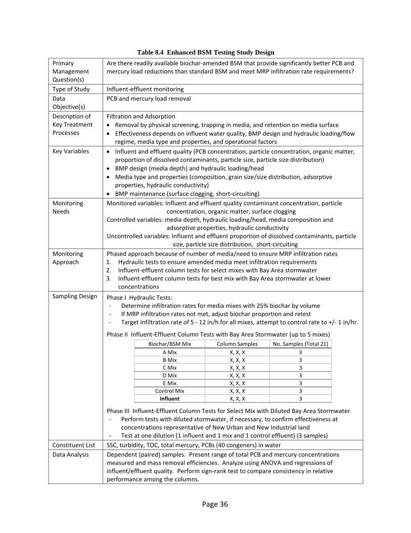
Page 36
Table 8.4 Enhanced BSM Testing Study Design
Primary Management Question(s)
Are there readily available biochar-amended BSM that provide significantly better PCB and mercury load reductions than standard BSM and meet MRP infiltration rate requirements?
Type of Study Influent-effluent monitoring
Data Objective(s)
PCB and mercury load removal
Description of Key Treatment Processes
Filtration and Adsorption
Removal by physical screening, trapping in media, and retention on media surface
Effectiveness depends on influent water quality, BMP design and hydraulic loading/flow regime, media type and properties, and operational factors
Key Variables Influent and effluent quality (PCB concentration, particle concentration, organic matter, proportion of dissolved contaminants, particle size, particle size distribution)
BMP design (media depth) and hydraulic loading/head
Media type and properties (composition, grain size/size distribution, adsorptive properties, hydraulic conductivity)
BMP maintenance (surface clogging, short-circuiting)
Monitoring Needs
Monitored variables: Influent and effluent quality contaminant concentration, particle concentration, organic matter, surface clogging
Controlled variables: media depth, hydraulic loading/head, media composition and adsorptive properties, hydraulic conductivity
Uncontrolled variables: Influent and effluent proportion of dissolved contaminants, particle size, particle size distribution, short-circuiting
Monitoring Approach
Phased approach because of number of media/need to ensure MRP infiltration rates 1. Hydraulic tests to ensure amended media meet infiltration requirements 2. Influent-effluent column tests for select mixes with Bay Area stormwater 3. Influent-effluent column tests for best mix with Bay Area stormwater at lower
concentrations
Sampling Design Phase I Hydraulic Tests: - Determine infiltration rates for media mixes with 25% biochar by volume - If MRP infiltration rates not met, adjust biochar proportion and retest - Target infiltration rate of 5 - 12 in/h for all mixes, attempt to control rate to +/- 1 in/hr.
Phase II Influent-Effluent Column Tests with Bay Area Stormwater (up to 5 mixes)
Biochar/BSM Mix Column Samples No. Samples (Total 21)
A Mix X, X, X 3
B Mix X, X, X 3
C Mix X, X, X 3
D Mix X, X, X 3
E Mix X, X, X 3
Control Mix X, X, X 3
Influent X, X, X 3
Phase III Influent-Effluent Column Tests for Select Mix with Diluted Bay Area Stormwater - Perform tests with diluted stormwater, if necessary, to confirm effectiveness at
concentrations representative of New Urban and New Industrial land - Test at one dilution (1 influent and 1 mix and 1 control effluent) (3 samples)
Constituent List SSC, turbidity, TOC, total mercury, PCBs (40 congeners) in water
Data Analysis Dependent (paired) samples. Present range of total PCB and mercury concentrations measured and mass removal efficiencies. Analyze using ANOVA and regressions of influent/effluent quality. Perform sign-rank test to compare consistency in relative performance among the columns.

Page 37
8.6 Adequacy of Study Design
The primary management questions are reviewed in this section in light of the budgeted data collection efforts. The primary management questions are restated and followed by an analysis of the adequacy of the data collection effort.
1. What are the annual PCB and mercury loads captured by existing HDS units in Bay Area urban watersheds?
Table 8.3 lists the number of data points that are anticipated for the HDS monitoring study.
This selected design will provide 9 data points for each of the following: PCB sediment concentration, mercury sediment concentration, and sediment mass. This design will not be able to assess the effect of HDS size and hydraulic loading on pollutant removal, and may not be able to statistically differentiate load capture between different land uses because of the small sample count for each land use (3). However, this design is selected because of the lack of information available on HDS sizing and the opportunistic nature of the sampling which limits the number of HDS units that can be sampled. The effect of maintenance is eliminated by ensuring that samples are not collected from units that have no remaining sump capacity.
The HDS study design collects independent (unpaired) samples since each HDS unit is sampled independently and there is no relationship between the various HDS units. This limits ability to discern differences due to land use or HDS size, especially when sample size is relatively low and there is considerable variability in the data collected. Although the study design yields 9 data points for each data objective, it may not be sufficient to draw statistically-based conclusions. However, the study will provide point estimates of loads removed during cleanouts and how they vary for different land uses (e.g., X g of PCBs are removed per unit area of Y land use). This is the metric used for effectiveness of HDS cleanouts, so the study will provide a practical improvement in knowledge that can be applied to future HDS effectiveness estimates.
In addition, modeled stormwater flows and associated POC loads to each HDS unit catchment during the time period between cleanouts will be developed. These modeled estimates will be used along with the measured mass captured in the HDS unit between cleanouts to quantify the percent removal for each unit during the study.
2. Are there readily available biochar-amended BSM that provide significantly better PCB and mercury load reductions than standard BSM and meet MRP infiltration rate requirements?
Table 8.4 lists the number of data points that are anticipated for the enhanced BSM testing study. The sampling design will yield 19 data points for each of the following: effluent PCB concentration, effluent mercury concentration. Including influent analysis, a total of 24 samples will be analyzed. The purpose of this study is to identify the best biochar amended BSM mixes for field testing and not test the effect of confounding variables such as influent quality and hydraulic loading on load removals. The study design accounts for these confounding variables by either ensuring their effect is randomized (e.g., influent water quality) or keeps them fixed (e.g., hydraulic loading). To ensure influent stormwater concentrations are representative of typical Bay Area concentrations, an additional column test with diluted

Page 38
stormwater is performed on an effective media mix. Standard BSM controls are used for each column run so that removal by biochar amended mixes can be compared directly to removal by standard BSM. Infiltration experiments are performed prior to the column testing to ensure media selected for final column testing will meet the MRP infiltration rate requirements.
The enhanced BSM column study design collects dependent (paired) samples since each effluent sample is related to a corresponding influent sample. Additionally, standard BSM controls are used for each run which makes it possible to directly compare effluent quality for each amended BSM to standard BSM. The paired sampling design, use of standard BSM controls, and ability to control or fix many of the variables that effect load removal increase the ability to discern differences in treatment. Therefore, only 3 column runs are proposed, and available budget is instead used in initial hydraulic screening experiments to ensure selected media mixes meet MRP infiltration rate requirements. The study design may not be sufficient to draw statistically-based conclusions because it yields only 3 data points for each biochar mix tested. However, the study will enable direct comparisons of effluent quality and treatment between mixes for individual events and consistency of treatment between events. The information provided by the study is expected to be sufficient to identify the most promising biochar mixes for field testing.
The study designs for the HDS monitoring and enhanced bioretention studies meet MRP sample collection requirements. The sampling design for the HDS monitoring study will yield a minimum of 9 PCB and mercury data points, while the sampling design for the enhanced bioretention laboratory study will yield 24 PCB and mercury data points (including influent analysis). The minimum number of PCB samples for this study plan is 33 (9+24). Because 3 of the 32 BMP effectiveness samples required by the current MRP have already been collected, the minimum number required for this project is 29. This study must yield 29 of the 32 permit-required samples, per Provision C.8.f of the MRP. To ensure that at least 29 samples are collected to meet the MRP requirement, additional samples will be collected during the laboratory media testing runs if fewer than 5 HDS units are available for sampling.

Page 39
9. Recommendations for Sampling
and Analysis Plans This section presents specific recommendations for the development of SAPs. More
detailed information is available in Section 6 of the Caltrans Monitoring Guidance Manual (Caltrans, 2015) and in the Urban Stormwater BMP Performance Monitoring (WERF 2009). Analysis of constituents should follow the CW4CB Quality Assurance Project Plan (BASMAA 2013).
9.1 HDS Monitoring
The following SAP recommendations are based on the lessons learned from sampling the Leo Avenue HDS site (BASMAA, 2017b):
Include equipment to determine sump capacity before sampling. The study design does not require sampling of units that are full (i.e., have no remaining sump capacity). The depth of the unit can make it difficult to inspect for sump basin contents, and use of a “sludge judge” or other similar equipment may not be possible because of difficulty penetrating through compacted organic materials.
The sampling is expected to be opportunistic sampling during regular cleanouts. Since it coincides with regular maintenance patterns, the occurrence of a clean and empty vactor truck from which samples of the sediment can be taken is unlikely. To obtain representative samples, multiple grab samples that extend from the top of the sediment layer to the bottom of the sump will need to be collected and composited prior to analyses.
Sediment samples will require screening to remove coarse particles, trash, etc. In the CW4CB study (BASMAA, 2007b), only sediment less than 2 mm in size was analyzed.
It is unclear how samples of the HDS sediment were taken in the Leo Avenue HDS sampling. Appropriate sampling methods should be developed to ensure the samples collected are representative of the sediment in the HDS units.
HDS sediment sampling is not expected to require additional handling/safety precautions beyond normal drain cleaning safety procedures. Human health criteria for PCBs are for exposure via ingestion or vapor intake and not for contact. OSHA directive STD 01-04-002 state that “repeated skin contact hazards with all PCB's could be addressed by the standards 1910.132 and 1910.133”. Both 1910.132 and 1910.133 OSHA standards require use of personal protective equipment, including eye and face protection.
9.2 Enhanced Bioretention Media Testing
The following SAP recommendations are based on past experience and specific guidance provided in DEMEAU (2014):
The enhanced BSM testing will use real stormwater for the column experiments to account for the effect of influent water quality on load removal. A stormwater

Page 40
collection site will need to be identified in a watershed with typical PCB concentrations to ensure PCB concentrations are representative of those expected in Bay Area urban watersheds. Also, guidance will need to be developed on mobilization to ensure storms are targeted randomly.
Stormwater properties are known to change significantly with time due to natural flocculation and settling of particles. Appropriate procedures should be developed to ensure collected stormwater is well mixed at all times, and experiments are performed in a timely manner to insure the stormwater used is representative.
PCBs can readily attach to test equipment, including the inside of tubing that may be used for pumps and the inside of PVC columns. Alternatives should be considered that eliminate the need for pumping equipment and reduce attachment within columns (e.g., by use of glass columns).
The results of column experiments can be affected by channeling and wall effects. Use a column diameter to particle diameter ratio greater than about 40 to minimize these.
How media is packed in columns will affect infiltration rates and treatment performance. Therefore, detailed procedures should be developed for the packing of media in columns to ensure consistency between columns and between experiments.
9.3 Data Quality Objectives
Data quality objectives (DQOs) should follow standard stormwater monitoring protocols and be described in detail in individual SAPs. Both sampling and laboratory data quality objectives should be included. For sampling, the SAP should specify sediment and water collection procedures and equipment as well as sample volume and handling requirements. For laboratories, numeric DQOs are appropriate for sample blanks, duplicates (or field splits), and matrix spike recovery.
Page 41
10. References BASMAA, 2013. Quality Assurance Project Plan (QAPP). Clean Watersheds for a Clean Bay –
Implementing the San Francisco Bay’s PCBs and Mercury TMDLs with a Focus on Urban Runoff. August
15, 2013.
BASMAA, 2014. Integrated Monitoring Report Part B: PCB and Mercury Loads Avoided and Reduced via
Stormwater Control Measures. Bay Area Stormwater Management Agencies Association.
BASMAA, 2016a. Regional Biotreatment Soil Specification: Specification of Soils for Biotreatment or
Bioretention Facilities. Bay Area Stormwater Management Agencies Association.
BASMAA, 2016b. Interim Accounting Methodology for TMDL Loads Reduced. Bay Area Stormwater
Management Agencies Association.
BASMAA, 2017a. Clean Watersheds for a Clean Bay Project Report, Final Report May 2017. Bay Area
Stormwater Management Agencies Association.
BASMAA, 2017b. Clean Watersheds for a Clean Bay Task 5: Stormwater Treatment Retrofit Pilot
Projects Stormwater Treatment Retrofit - 7th Street Hydrodynamic Separator Unit draining the Leo
Avenue Watershed, San Jose, CA. Bay Area Stormwater Management Agencies Association.
BASMAA, 2017c. Bay Area Reasonable Assurance Analysis Guidance Document. Project Number:
WW2282, June 2017. Bay Area Stormwater Management Agencies Association.
Caltrans, 2009. BMP Pilot Study Guidance Manual. Document No. CTSW-RT-06-171.02.1. California
Department of Transportation, Sacramento.
Caltrans, 2015. Caltrans Stormwater Monitoring Guidance Manual, November 2015. Document No.
CTSW-OT-15-999.43.01. California Department of Transportation, Sacramento.
City of San Diego, 2012. Catch Basin Inlet Cleaning Pilot Study Final Report, June 2012. The City of San
Diego, California.
City of Spokane, 2015. PCB Characterization of Spokane Regional Vactor Waste Decant Facilities,
Prepared for the Spokane River Regional Toxics Taskforce September, 2015. City of Spokane RPWRF
Laboratory.
City of Tacoma, 2015. East Tacoma PCB Investigation: Results & Next Steps. November 20, 2013. City
of Tacoma Environmental Services.
City of Tacoma PCB Presentation. Last Assessed May 28, 2017.
DEMEAU, 2014. Guidelining protocol for soil-column experiments assessing fate and transport of trace
organics. Demonstration of promising technologies to address emerging pollutants in water and waste
water project. European Union Seventh Programme for Research, Technological Development and
Demonstration under Grant Agreement No. 308330.

Page 42
Gomez-Eyles, J. L., C. Yupanqui, B. Beckingham, G. Riedel, C. Gilmour, and U. Ghosh, 2013. Evaluation of
Biochars and Activated Carbons for In Situ Remediation of Sediments Impacted with Organics, Mercury,
and Methylmercury. Environ. Sci. Technol., 47, 13721−13729.
Kitsap County, 2015. Analysis of Bioretention Soil Media for Improved Nitrogen, Phosphorus and
Copper Retention, Final Report. Kitsap County Public Works, Washington.
Liu, P., C. J. Ptacek, D. W. Blowes, and R. C. Landis, 2015. Mechanisms of mercury removal by biochars
produced from different feedstocks determined using X-ray absorption spectroscopy. Journal of
Hazardous Materials, 308 (2016) 233–242.
SFBRWQCB, 2012. San Francisco Bay Regional Water Quality Control Board. Total Maximum Daily Loads
(TMDLs) and the 303(d) List of Impaired Water Bodies. 2012.
SFBRWQCB, 2015. Municipal Regional Stormwater NPDES Permit, Order No. R2-2015-0049. NPDES
Permit No. CAS612008. November 19, 2015
SFEI, 2015. Sources, Pathways and Loadings: Multi-Year Synthesis with a Focus on PCBs and Hg. Report
for Regional Monitoring Program for Water Quality in San Francisco Bay (RMP), Sources Pathways and
Loadings Workgroup (SPLWG), Small Tributaries Loading Strategy (STLS). 2015.
WERF, 2009. Urban Stormwater BMP Performance Monitoring. Water Environment Research Foundation. Urban Stormwater BMP Performance Monitoring. Last accessed August 6, 2012.
Wilson M. A., O. Mohseni, J. S. Gulliver, R. M. Hozalski, and H. G. Stefan, 2009. Assessment of
Hydrodynamic Separators for Storm-Water Treatment. J. Hydraul. Eng., 2009, 135(5): 383-392.
Yargicoglu, E. N. and K. R. Reddy, 2015. Characterization and Surface Analysis of Commercially Available
Biochars for Geoenvironmental Applications. IFCEE2015, San Antonio, TX, March 17-21, 2015.
Yee, D., and L. J. McKee, 2010. Task 3.5: Concentrations of PCBs and Hg in soils, sediments and water in
the urbanized Bay Area: Implications for best management. A technical report of the Watershed
Program. SFEI Contribution 608. San Francisco Estuary Institute, Oakland CA.

Final Project Report – POC Removal Effectiveness of HDS Units 2019
APPENDIX B: SAMPLING AND ANALYSIS PLAN AND QUALITY ASSURANCE
PROJECT PLAN

BASMAA Regional Monitoring Coalition Pollutants of Concern Monitoring for Source Identification and Management Action Effectiveness, 2017-2018 Sampling and Analysis Plan and Quality Assurance Project Plan
Prepared for:
The Bay Area Stormwater Management Agencies Association (BASMAA)
Prepared by:
1410 Jackson Street 6000 J Street 4911 Central Avenue 307 Washington Street
Oakland, CA Sacramento, CA Richmond, CA Santa Cruz, CA
94612 95819 94804 95060
Version 2 September 29, 2017

BASMAA POC Monitoring for Source Identification and Management Action Effectiveness Sampling and Analysis Plan and Quality Assurance Project Plan
Version 2, September 2017
2
Title and Approval Sheet
Program Title Pollutants of Concern (POC) Monitoring for Source Identification
and Management Action Effectiveness
Lead Organization Bay Area Stormwater Management Agencies Association (BASMAA)
P.O. Box 2385, Menlo Park, CA 94026, 510-622-2326
Primary Contact Geoff Brosseau
Effective Date September 29, 2017
Revision Number Version 2
Approval Signatures:
A signature from the BASMAA Executive Director approving the BASMAA POC Monitoring for Source Identification and
Management Action Effectiveness is considered approval on behalf of all Program Managers.
Geoff Brosseau Date

BASMAA POC Monitoring for Source Identification and Management Action Effectiveness Sampling and Analysis Plan and Quality Assurance Project Plan
Version 2, September 2017
3
TABLE OF CONTENTS
TITLE AND APPROVAL SHEET ........................................................................................................................... 2 APPROVAL SIGNATURES: ....................................................................................................................................................... 2
1. PROBLEM DEFINITION/BACKGROUND ........................................................................................... 9 1.1. PROBLEM STATEMENT ........................................................................................................................................... 9 1.2. OUTCOMES .............................................................................................................................................................. 10
2. DISTRIBUTION LIST AND CONTACT INFORMATION ................................................................ 11
3. PROGRAM ORGANIZATION ............................................................................................................... 11 3.1. INVOLVED PARTIES AND ROLES.......................................................................................................................... 11 3.2. BASMAA PROJECT MANAGER (BASMAA-PM) ............................................................................................ 12 3.3. BASMAA PROJECT MANAGEMENT TEAM (PMT) .......................................................................................... 13 3.4. CONSULTANT TEAM PROJECT MANAGER (CONSULTANT-PM) .................................................................... 13 3.5. QUALITY ASSURANCE OFFICER (QA OFFICER) ................................................................................................ 13 3.6. DATA MANAGER (DM) ........................................................................................................................................ 13 3.7. FIELD CONTRACTOR PROJECT MANAGER (FIELD-PM) ................................................................................. 13 3.8. LABORATORY PROJECT MANAGER (LAB-PM) ................................................................................................. 14 3.1. REPORT PREPARER ............................................................................................................................................... 14
4. MONITORING PROGRAM DESCRIPTION ....................................................................................... 14 4.1. WORK STATEMENT AND PROGRAM OVERVIEW .............................................................................................. 14 4.2. SAMPLING DETAIL ................................................................................................................................................. 15
4.2.1. Task 1 - Caulk/Sealant samples .................................................................................................................... 15 4.2.2. Task 2 - Sediment samples from HDS Units ............................................................................................. 16 4.2.3. Task 3 - Storm Water and Column Test Samples .................................................................................. 16
4.3. SCHEDULE ............................................................................................................................................................... 17 4.4. GEOGRAPHICAL SETTING ..................................................................................................................................... 17 4.5. CONSTRAINTS ........................................................................................................................................................ 17
5. MEASUREMENT QUALITY OBJECTIVES (MQO) .......................................................................... 18 5.1. REPRESENTATIVENESS AND COMPARABILITY ................................................................................................. 18 5.2. COMPLETENESS ..................................................................................................................................................... 19 5.3. SENSITIVITY ........................................................................................................................................................... 19 5.4. PRECISION .............................................................................................................................................................. 19 5.5. ACCURACY............................................................................................................................................................... 20 5.6. CONTAMINATION ................................................................................................................................................... 20
6. SPECIAL TRAINING NEEDS / CERTIFICATION ............................................................................ 21
7. PROGRAM DOCUMENTATION AND REPORTING ....................................................................... 21 7.1. FIELD DOCUMENTATION ...................................................................................................................................... 22
7.1.1. Sampling Plans, COCs, and Sampling Reports ........................................................................................ 22 7.1.2. Data Sheets ............................................................................................................................................................. 22 7.1.3. Photographic Documentation ........................................................................................................................ 22
7.2. LABORATORY DOCUMENTATION ........................................................................................................................ 22 7.2.1. Data Reporting Format ..................................................................................................................................... 22 7.2.2. Other Laboratory QA/QC Documentation ................................................................................................ 23
7.3. PROGRAM MANAGEMENT DOCUMENTATION ................................................................................................... 24 7.3.1. SAP/QAPP ................................................................................................................................................................ 24 7.3.2. Program Information Archival ...................................................................................................................... 24
7.4. REPORTING ............................................................................................................................................................. 25
BASMAA POC Monitoring for Source Identification and Management Action Effectiveness Sampling and Analysis Plan and Quality Assurance Project Plan
Version 2, September 2017
4
8. SAMPLING PROCESS DESIGN ............................................................................................................ 25 8.1. CAULK/SEALANT SAMPLING ............................................................................................................................... 25 8.2. SEDIMENT QUALITY SAMPLING .......................................................................................................................... 25 8.3. WATER QUALITY SAMPLING ............................................................................................................................... 26 8.4. SAMPLING UNCERTAINTY .................................................................................................................................... 26
9. SAMPLING METHODS .......................................................................................................................... 26 9.1. CAULK/SEALANT SAMPLING (TASK 1) ............................................................................................................. 27
9.1.1. Sample Site Selection .......................................................................................................................................... 27 9.1.2. Initial Equipment Cleaning ............................................................................................................................. 27 9.1.3. Field Cleaning Protocol ..................................................................................................................................... 27 9.1.4. Blind Sampling Procedures ............................................................................................................................. 27 9.1.5. Caulk/Sealant Collection Procedures ......................................................................................................... 28 9.1.6. Sample ID Designation ...................................................................................................................................... 29
9.2. HDS UNIT SAMPLING PROCEDURES (TASK 2) ................................................................................................ 29 9.2.1. Sample Site Selection .......................................................................................................................................... 29 9.2.2. Field Equipment and Cleaning ....................................................................................................................... 29 9.2.3. Soil / Sediment Sample Collection ............................................................................................................... 30 9.2.4. Sample ID Designation ...................................................................................................................................... 31
9.3. WATER QUALITY SAMPLING AND COLUMN TESTING PROCEDURES (TASK 3) .......................................... 32 9.3.1. Sample Site Selection .......................................................................................................................................... 32 9.3.2. Field Equipment and Cleaning ....................................................................................................................... 32 9.3.3. Water Sampling Procedures ........................................................................................................................... 32 9.3.4. Hydraulic Testing ................................................................................................................................................. 32 9.3.5. Column Testing Procedures ............................................................................................................................ 33 9.3.6. Sample ID Designations .................................................................................................................................... 34
9.4. COLLECTION OF SAMPLES FOR ARCHIVING ....................................................................................................... 35 9.5. WASTE DISPOSAL .................................................................................................................................................. 35
9.5.1. Routine Garbage ................................................................................................................................................... 35 9.5.2. Detergent Washes ................................................................................................................................................ 35 9.5.3. Chemicals ................................................................................................................................................................. 35
9.1. RESPONSIBILITY AND CORRECTIVE ACTIONS ................................................................................................... 35 9.2. STANDARD OPERATING PROCEDURES ............................................................................................................... 35
10. SAMPLE HANDLING AND CUSTODY................................................................................................ 36 10.1. SAMPLING CONTAINERS ....................................................................................................................................... 36 10.2. SAMPLE PRESERVATION ...................................................................................................................................... 37 10.3. PACKAGING AND SHIPPING .................................................................................................................................. 37 10.4. COMMERCIAL VEHICLE TRANSPORT .................................................................................................................. 37 10.5. SAMPLE HOLD TIMES ........................................................................................................................................... 37
11. FIELD HEALTH AND SAFETY PROCEDURES ................................................................................ 39
12. LABORATORY ANALYTICAL METHODS ........................................................................................ 39 12.1. CAULK/SEALANT SAMPLES (TASK 1) ............................................................................................................... 39
12.1.1. XRF Chlorine analysis ................................................................................................................................... 39 12.1.2. Selection of Samples for PCB analysis and Compositing .............................................................. 39 12.1.3. Sample Preparation ...................................................................................................................................... 40 12.1.4. PCBs Analysis .................................................................................................................................................... 40
12.2. SEDIMENT SAMPLES COLLECTED FROM HDS UNITS (TASK 2) .................................................................... 41 12.3. WATER SAMPLES – STORMWATER AND COLUMN TESTS (TASK 3) ............................................................. 41 12.4. METHOD FAILURES ............................................................................................................................................... 41

BASMAA POC Monitoring for Source Identification and Management Action Effectiveness Sampling and Analysis Plan and Quality Assurance Project Plan
Version 2, September 2017
5
12.5. SAMPLE DISPOSAL................................................................................................................................................. 42 12.6. LABORATORY SAMPLE PROCESSING .................................................................................................................. 42
13. QUALITY CONTROL .............................................................................................................................. 42 13.1. FIELD QUALITY CONTROL .................................................................................................................................... 42
13.1.1. Field Blanks ....................................................................................................................................................... 43 13.1.2. Field Duplicates ............................................................................................................................................... 43 13.1.3. Field Corrective Action ................................................................................................................................. 43
13.2. LABORATORY QUALITY CONTROL ...................................................................................................................... 44 13.2.1. Calibration and Working Standards ..................................................................................................... 45 13.2.2. Instrument Calibration ................................................................................................................................ 45 13.2.3. Initial Calibration Verification ................................................................................................................. 45 13.2.4. Continuing Calibration Verification ...................................................................................................... 45 13.2.5. Laboratory Blanks ......................................................................................................................................... 46 13.2.6. Reference Materials and Demonstration of Laboratory Accuracy.......................................... 46 13.2.7. Reference Materials vs. Certified Reference Materials .................................................................. 46 13.2.8. Laboratory Control Samples ..................................................................................................................... 47 13.2.9. Prioritizing Certified Reference Materials, Reference Materials, and Laboratory Control Samples ..................................................................................................................................................................... 47 13.2.10. Matrix Spikes .................................................................................................................................................... 47 13.2.11. Laboratory Duplicates ................................................................................................................................. 48 13.2.12. Laboratory Duplicates vs. Matrix Spike Duplicates ........................................................................ 48 13.2.13. Replicate Analyses .......................................................................................................................................... 48 13.2.14. Surrogates .......................................................................................................................................................... 48 13.2.15. Internal Standards ......................................................................................................................................... 48 13.2.16. Dual-Column Confirmation ........................................................................................................................ 49 13.2.17. Dilution of Samples ........................................................................................................................................ 49 13.2.18. Laboratory Corrective Action ................................................................................................................... 49
14. INSPECTION/ACCEPTANCE FOR SUPPLIES AND CONSUMABLES ........................................ 56
15. NON DIRECT MEASUREMENTS, EXISTING DATA ....................................................................... 56
16. DATA MANAGEMENT .......................................................................................................................... 56 16.1. FIELD DATA MANAGEMENT ................................................................................................................................ 56 16.2. LABORATORY DATA MANAGEMENT .................................................................................................................. 56
17. ASSESSMENTS AND RESPONSE ACTIONS ..................................................................................... 57 17.1. READINESS REVIEWS ............................................................................................................................................ 57 17.2. POST SAMPLING EVENT REVIEWS ...................................................................................................................... 57 17.3. LABORATORY DATA REVIEWS ............................................................................................................................ 57
18. INSTRUMENT/EQUIPMENT TESTING, INSPECTION AND MAINTENANCE ........................ 58 18.1. FIELD EQUIPMENT ................................................................................................................................................ 58 18.2. LABORATORY EQUIPMENT .................................................................................................................................. 58
19. INSTRUMENT/EQUIPMENT CALIBRATION AND FREQUENCY .............................................. 59 19.1. FIELD MEASUREMENTS ........................................................................................................................................ 59 19.2. LABORATORY ANALYSES ...................................................................................................................................... 59
19.2.1. In-house Analysis – XRF Screening ......................................................................................................... 59 19.2.2. Contract Laboratory Analyses .................................................................................................................. 59
20. DATA REVIEW, VERIFICATION, AND VALIDATION ................................................................... 60
21. VERIFICATION AND VALIDATION METHODS ............................................................................. 61

BASMAA POC Monitoring for Source Identification and Management Action Effectiveness Sampling and Analysis Plan and Quality Assurance Project Plan
Version 2, September 2017
6
22. RECONCILIATION WITH USER REQUIREMENTS ........................................................................ 61
23. REFERENCES ........................................................................................................................................... 62
24. APPENDIX A: FIELD DOCUMENTATION ....................................................................................... 63
25. APPENDIX B: LABORATORY STANDARD OPERATING PROCEDURES (SOPS) ................. 69
List of Tables
TABLE 2-1. BASMAA SAP/QAPP DISTRIBUTION LIST. .......................................................................................................................... 11 TABLE 3-1. SAN FRANCISCO BAY AREA STORMWATER PROGRAMS AND ASSOCIATED MRP PERMITTEES PARTICIPATING IN THE
BASMAA MONITORING PROGRAM. .................................................................................................................................................... 12 TABLE 7-1. DOCUMENT AND RECORD RETENTION, ARCHIVAL, AND DISPOSITION ............................................................................... 24 TABLE 7-2. MONITORING PROGRAM FINAL REPORTING DUE DATES. ........................................................................................... 25 TABLE 9-1 FIELD EQUIPMENT FOR HDS UNIT SAMPLING. ........................................................................................................................ 30 TABLE 9-2 STATION CODES FOR STORMWATER INFLUENT SAMPLES AND COLUMN TESTS. ............................................................... 35 TABLE 9-3. LIST OF BASMAA RMC SOPS UTILIZED BY THE MONITORING PROGRAM....................................................................... 36 TABLE 10-1 SAMPLE HANDLING FOR THE MONITORING PROGRAM ANALYTES BY MEDIA TYPE. ....................................................... 38 TABLE 12-1. LABORATORY ANALYTICAL METHODS FOR ANALYTES IN SEDIMENT ............................................................................... 41 TABLE 12-2. LABORATORY ANALYTICAL METHODS FOR ANALYTES IN WATER .................................................................................... 41 TABLE 13-1. MEASUREMENT QUALITY OBJECTIVES - PCBS. .................................................................................................................... 50 TABLE 13-2. MEASUREMENT QUALITY OBJECTIVES – INORGANIC ANALYTES. ...................................................................................... 51 TABLE 13-3. MEASUREMENT QUALITY OBJECTIVES – CONVENTIONAL ANALYTES. ............................................................................. 52 TABLE 13-4. TARGET MRLS FOR SEDIMENT QUALITY PARAMETERS. .................................................................................................... 52 TABLE 13-5. TARGET MRLS FOR PCBS IN WATER, SEDIMENT AND CAULK .......................................................................................... 53 TABLE 13-6. SIZE DISTRIBUTION CATEGORIES FOR GRAIN SIZE IN SEDIMENT ...................................................................................... 54 TABLE 13-7. TARGET MRLS FOR TOC, SSC, AND MERCURY IN WATER ................................................................................................ 54 TABLE 13-8. CORRECTIVE ACTION – LABORATORY AND FIELD QUALITY CONTROL ............................................................................. 55 TABLE 14-1. INSPECTION / ACCEPTANCE TESTING REQUIREMENTS FOR CONSUMABLES AND SUPPLIES ......................................... 56

BASMAA POC Monitoring for Source Identification and Management Action Effectiveness Sampling and Analysis Plan and Quality Assurance Project Plan
Version 2, September 2017
7
List of Acronyms
ACCWP Alameda Countywide Clean Water Program
ALS ALS Environmental Laboratory
BASMAA Bay Area Stormwater Management Agencies Association
BSM Bioretention Soil Media
CCCWP Contra Costa Clean Water Program
CCV continuing calibration verification
CEDEN California Environmental Data Exchange Network
CEH Center for Environmental Health
COC Chain of Custody
Consultant-PM Consultant Team Project Manager
CRM Certified Reference Material
CSE Confined Space Entry
ECD Electron capture detection
EDD Electronic Data Deliverable
EOA Eisenberg, Olivieri & Associates, Inc.
EPA Environmental Protection Agency (U.S.)
FD Field duplicate
Field PM Field Contractor Project Manager
FSURMP Fairfield-Suisun Urban Runoff Management Program
GC-MS Gas Chromatography-Mass Spectroscopy
IDL Instrument Detection Limits
ICV initial calibration verification
KLI Kinnetic Laboratories Inc.
LCS Laboratory Control Samples
Lab-PM Laboratory Project Manager
MS/MSD Matrix Spike/Matrix Spike Duplicate
MDL Method Detection Limit
MQO Measurement Quality Objective
MRL Method Reporting Limit
MRP Municipal Regional Permit
NPDES National Pollutant Discharge Elimination System
OWP-CSUS Office of Water Programs at California State University Sacramento
PCB Polychlorinated Biphenyl
PM Project Manager
PMT Project Management Team
POC Pollutants of Concern
QA Quality Assurance
QA Officer Quality Assurance Officer
QAPP Quality Assurance Project Plan
QC Quality Control
ROW Right-of-way
RPD Relative Percent Difference
RMC Regional Monitoring Coalition
RMP Regional Monitoring Program for Water Quality in the San Francisco Estuary
SFRWQCB San Francisco Regional Water Quality Control Board (Regional Water Board)
SAP Sampling and Analysis Plan
SCCVURPP Santa Clara Valley Urban Runoff Pollution Prevention Program
SCVWD Santa Clara Valley Water Department
SFEI San Francisco Estuary Institute

BASMAA POC Monitoring for Source Identification and Management Action Effectiveness Sampling and Analysis Plan and Quality Assurance Project Plan
Version 2, September 2017
8
SMCWPPP San Mateo County Water Pollution Prevention Program
SOP Standard Operating Procedure
SWAMP California Surface Water Ambient Monitoring Program
TOC Total Organic Carbon
TMDL Total Maximum Daily Load
VSFCD Vallejo Sanitation and Flood Control District

BASMAA POC Monitoring for Source Identification and Management Action Effectiveness Sampling and Analysis Plan and Quality Assurance Project Plan
Version 2, September 2017
9
1. Problem Definition/Background The Bay Area Stormwater Management Agencies Association (BASMAA) member agencies will
implement a regional monitoring program for Pollutants of Concern (POC) Monitoring for Source
Identification and Management Action Effectiveness (Monitoring Program). The Monitoring Program is
intended to fulfill components of the Municipal Regional Stormwater NPDES Permit (MRP; Order No.
R2-2015-0049), which implements the polychlorinated biphenyls (PCBs) and Mercury Total Maximum
Daily Loads (TMDLs) for the San Francisco Bay Area. Monitoring for Source Identification and
Management Action Effectiveness are two of five monitoring priorities for POCs identified in the MRP.
Source identification monitoring is conducted to identify the sources or watershed source areas that
provide the greatest opportunities for reductions of POCs in urban stormwater runoff. Management action
effectiveness monitoring is conducted to provide support for planning future management actions or to
evaluate the effectiveness or impacts of existing management actions.
BASMAA developed two study designs to implement each component of the Monitoring Program. The
Evaluation of PCBs Presence in Public Roadway and Storm Drain Infrastructure Caulk and Sealants
Study Design (BASMAA 2017a) addresses the source identification monitoring requirements of
Provision C.8.f, as well as requirements of Provision C.12.e to investigate PCBs in infrastructure caulk
and sealants. The POC Monitoring for Management Action Effectiveness Study Design (BASMAA
2017b) addresses the management action effectiveness monitoring requirements of Provision C.8.f. The
results of the Monitoring Program will contribute to ongoing efforts by MRP Permittees to identify PCB
sources and improve the PCBs and mercury treatment effectiveness of stormwater control measures in the
Phase I permittee area of the Bay Area. This Sampling and Analysis Plan and Quality Assurance Project
Plan (SAP/QAPP) was developed to guide implementation of both components of the Monitoring
Program.
1.1. Problem Statement
Fish tissue monitoring in San Francisco Bay (Bay) has revealed bioaccumulation of PCBs and mercury.
The measured fish tissue concentrations are thought to pose a health risk to people consuming fish caught
in the Bay. As a result of these findings, California has issued an interim advisory on the consumption of
fish from the Bay. The advisory led to the Bay being designated as an impaired water body on the Clean
Water Act "Section 303(d) list" due to PCBs and mercury. In response, the California Regional Water
Quality Control Board, San Francisco Bay Region (Regional Water Board) has developed TMDL water
quality restoration programs targeting PCBs and mercury in the Bay. The general goals of the TMDLs are
to identify sources of PCBs and mercury to the Bay and implement actions to control the sources and
restore water quality.
Since the TMDLs were adopted, Permittees have conducted a number of projects to provide information
that supports implementation of management actions designed to achieve the wasteload allocations
described in the Mercury and PCBs TMDL, as required by Provisions of the MRP. The Clean Watersheds
for a Clean Bay project (CW4CB) was a collaboration among BASMAA member agencies that pilot
tested various stormwater control measures and provided estimates of the PCBs and mercury load
reduction effectiveness of these controls (BASMAA, 2017c). However, the results of the CW4CB project
identified a number of remaining data gaps on the load reduction effectiveness of the control measures

BASMAA POC Monitoring for Source Identification and Management Action Effectiveness Sampling and Analysis Plan and Quality Assurance Project Plan
Version 2, September 2017
10
that were tested. In addition, MRP Provisions C.8.f. and C.12.e require Permittees to conduct further
source identification and management action effectiveness monitoring during the current permit term.
1.2. Outcomes
The Monitoring Program will allow Permittees to satisfy MRP monitoring requirements for source
identification and management action effectiveness, while also addressing some of the data gaps
identified by the CW4CB project (BASMAA, 2017c). Specifically, the Monitoring Program is intended
to provide the following outcomes:
1. Satisfy MRP Provision C.8.f. requirements for POC monitoring for source identification; and
Satisfy MRP Provision C.12.e.ii requirements to evaluate PCBs presence in caulks/sealants used
in storm drain or roadway infrastructure in public ROWs;
a. Report the range of PCB concentrations observed in 20 composite samples of
caulk/sealant collected from structures installed or rehabilitated during the 1970’s;
2. Satisfy MRP Provision C.8.f. requirements for POC monitoring for management action
effectiveness;
a. Quantify the annual mass of mercury and PCBs captured in HDS Unit sumps during
maintenance; and
b. Identify bioretention soil media (BSM) mixtures for future field testing that provide the
most effective mercury and PCBs treatment in laboratory column tests.
The information generated from the Monitoring Program will be used by MRP Permittees and the
Regional Water Board to better understand potential PCB sources and better estimate the load reduction
effectiveness of current and future stormwater control measures.
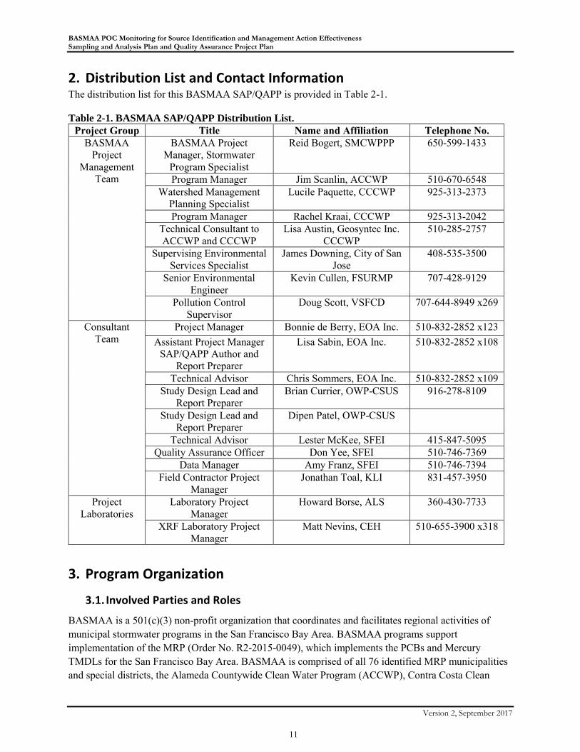
BASMAA POC Monitoring for Source Identification and Management Action Effectiveness Sampling and Analysis Plan and Quality Assurance Project Plan
Version 2, September 2017
11
2. Distribution List and Contact Information The distribution list for this BASMAA SAP/QAPP is provided in Table 2-1.
Table 2-1. BASMAA SAP/QAPP Distribution List.
Project Group Title Name and Affiliation Telephone No.
BASMAA
Project
Management
Team
BASMAA Project
Manager, Stormwater
Program Specialist
Reid Bogert, SMCWPPP 650-599-1433
Program Manager Jim Scanlin, ACCWP 510-670-6548
Watershed Management
Planning Specialist
Lucile Paquette, CCCWP 925-313-2373
Program Manager Rachel Kraai, CCCWP 925-313-2042
Technical Consultant to
ACCWP and CCCWP
Lisa Austin, Geosyntec Inc.
CCCWP
510-285-2757
Supervising Environmental
Services Specialist
James Downing, City of San
Jose
408-535-3500
Senior Environmental
Engineer
Kevin Cullen, FSURMP 707-428-9129
Pollution Control
Supervisor
Doug Scott, VSFCD 707-644-8949 x269
Consultant
Team
Project Manager Bonnie de Berry, EOA Inc. 510-832-2852 x123
Assistant Project Manager
SAP/QAPP Author and
Report Preparer
Lisa Sabin, EOA Inc. 510-832-2852 x108
Technical Advisor Chris Sommers, EOA Inc. 510-832-2852 x109
Study Design Lead and
Report Preparer
Brian Currier, OWP-CSUS 916-278-8109
Study Design Lead and
Report Preparer
Dipen Patel, OWP-CSUS
Technical Advisor Lester McKee, SFEI 415-847-5095
Quality Assurance Officer Don Yee, SFEI 510-746-7369
Data Manager Amy Franz, SFEI 510-746-7394
Field Contractor Project
Manager
Jonathan Toal, KLI 831-457-3950
Project
Laboratories
Laboratory Project
Manager
Howard Borse, ALS 360-430-7733
XRF Laboratory Project
Manager
Matt Nevins, CEH 510-655-3900 x318
3. Program Organization
3.1. Involved Parties and Roles
BASMAA is a 501(c)(3) non-profit organization that coordinates and facilitates regional activities of
municipal stormwater programs in the San Francisco Bay Area. BASMAA programs support
implementation of the MRP (Order No. R2-2015-0049), which implements the PCBs and Mercury
TMDLs for the San Francisco Bay Area. BASMAA is comprised of all 76 identified MRP municipalities
and special districts, the Alameda Countywide Clean Water Program (ACCWP), Contra Costa Clean

BASMAA POC Monitoring for Source Identification and Management Action Effectiveness Sampling and Analysis Plan and Quality Assurance Project Plan
Version 2, September 2017
12
Water Program (CCCWP), the Santa Clara Valley Urban Runoff Pollution Prevention Program
(SCVURPPP), the San Mateo Countywide Water Pollution Prevention Program (SMCWPPP), the
Fairfield-Suisun Urban Runoff Management Program (FSURMP), the City of Vallejo and the Vallejo
Sanitation and Flood Control District (VSFCD) (Table 3-1).
MRP Permittees have agreed to collectively implement this Monitoring Program via BASMAA. The
Program will be facilitated through the BASMAA Monitoring and Pollutants of Concern Committee
(MPC). BASMAA selected a consultant team to develop and implement the Monitoring Program with
oversight and guidance from a BASMAA Project Management Team (PMT), consisting of
representatives from BASMAA stormwater programs and municipalities (Table 3-1).
Table 3-1. San Francisco Bay Area Stormwater Programs and Associated MRP Permittees
Participating in the BASMAA Monitoring Program.
3.2. BASMAA Project Manager (BASMAA-PM)
The BASMAA Project Manager (BASMAA-PM) will be responsible for directing the activities of the
below-described PMT, and will provide oversight and managerial level activities, including reporting
status updates to the PMT and BASMAA, and acting as the liaison between the PMT and the Consultant
Team. The BASMAA PM will oversee preparation, review, and approval of project deliverables,
including the required reports to the Regional Water Board.
Stormwater Programs MRP Permittees
Santa Clara Valley Urban Runoff
Pollution Prevention Program
(SCVURPPP)
Cities of Campbell, Cupertino, Los Altos, Milpitas, Monte Sereno,
Mountain View, Palo Alto, San Jose, Santa Clara, Saratoga,
Sunnyvale, Los Altos Hills, and Los Gatos; Santa Clara Valley
Water District; and, Santa Clara County
Alameda Countywide Clean
Water Program (ACCWP)
Cities of Alameda, Albany, Berkeley, Dublin, Emeryville,
Fremont, Hayward, Livermore, Newark, Oakland, Piedmont,
Pleasanton, San Leandro, and Union City; Alameda County;
Alameda County Flood Control and Water Conservation District;
and, Zone 7 Water District
Contra Costa Clean Water
Program (CCCWP)
Cities of, Clayton, Concord, El Cerrito, Hercules, Lafayette,
Martinez, , Orinda, Pinole, Pittsburg, Pleasant Hill, Richmond,
San Pablo, San Ramon, Walnut Creek, Danville, and Moraga;
Contra Costa County; and, Contra Costa County Flood Control
and Water Conservation District
San Mateo County Wide Water
Pollution Prevention Program
(SMCWPPP)
Cities of Belmont, Brisbane, Burlingame, Daly City, East Palo
Alto, Foster City, Half Moon Bay, Menlo Park, Millbrae, Pacifica,
Redwood City, San Bruno, San Carlos, San Mateo, South San
Francisco, Atherton, Colma, Hillsborough, Portola Valley, and
Woodside; San Mateo County Flood Control District; and, San
Mateo County
Fairfield-Suisun Urban Runoff
Management Program (FSURMP)
Cities of Fairfield and Suisun City
Vallejo Permittees (VSFCD) City of Vallejo and Vallejo Sanitation and Flood Control District

BASMAA POC Monitoring for Source Identification and Management Action Effectiveness Sampling and Analysis Plan and Quality Assurance Project Plan
Version 2, September 2017
13
3.3. BASMAA Project Management Team (PMT)
The BASMAA PMT will assist the BASMAA-PM and the below described Consultant Team with the
design and implementation of all project activities. PMT members will assist the BASMAA-PM and
Consultant Team to complete project activities within scope, on-time, and within budget by having
specific responsibility for planning and oversight of project activities within the jurisdiction of the
BASMAA agency that they represent. In addition, the PMT will coordinate with the municipal project
partners and key regional agencies, including the Regional Water Board. The PMT is also responsible for
reviewing and approving project deliverables (e.g., draft and final project reports).
3.4. Consultant Team Project Manager (Consultant-PM)
The Consultant Team Project Manager (Consultant-PM) will be responsible for ensuring all work
performed during the Monitoring Program is consistent with project goals, and provide oversight of all
day-to-day operations associated with implementing all components of the Monitoring Program,
including scheduling, budgeting, reporting, and oversight of subcontractors. The Consultant-PM will
ensure that data generated and reported through implementation of the Monitoring Program meet
measurement quality objectives (MQOs) described in this SAP/QAPP. The Consultant -PM will work
with the Quality Assurance Officer as required to resolve any uncertainties or discrepancies. The
Consultant -PM will also be responsible for overseeing development of draft and final reports for the
Monitoring Program, as described in this SAP/QAPP.
3.5. Quality Assurance Officer (QA Officer)
The role of the Quality Assurance Officer (QA Officer) is to provide independent oversight and review of
the quality of the data being generated. In this role, the QA Officer has the responsibility to require data
that is of insufficient quality to be flagged, or not used, or for work to be redone as necessary so that the
data meets specified quality measurements. The QA Officer will oversee the technical conduct of the field
related components of the Monitoring Program, including ensuring field program compliance with the
SAP/QAPP for tasks overseen at the programmatic level.
3.6. Data Manager (DM)
The Data Manager will be responsible for receipt and review of all project related documentation and
reporting associated with both field efforts and laboratory analysis. The Data Manager will also be
responsible for storage and safekeeping of these records for the duration of the project.
3.7. Field Contractor Project Manager (Field-PM)
The Field Contractor Project Manager (Field-PM) will be responsible for conduct and oversight of all
field monitoring- and reporting-related activities, including completion of field datasheets, chain of
custodies, and collection of field measurements and field samples, consistent with the monitoring
methods and procedures in the SAP/QAPP. The Field-PM will also be responsible for ensuring that
personnel conducting monitoring are qualified to perform their responsibilities and have received
appropriate training. The Field-PM will be responsible for initial receipt and review of all project related
documentation and reporting associated with both field efforts and laboratory analysis.

BASMAA POC Monitoring for Source Identification and Management Action Effectiveness Sampling and Analysis Plan and Quality Assurance Project Plan
Version 2, September 2017
14
The Field-PM will also be responsible for receiving all samples collected opportunistically by
participating municipalities, including all caulk/sealant samples, initial review of sample IDs to ensure
there are no duplicate sample IDs, and shipping the samples under COC to the appropriate laboratory
(CEH for the caulk/sealant samples; ALS for all other samples). Participating municipalities should ship
all samples they collect to the Field PM at the following address:
Jon Toal
Kinnetic Laboratories, Inc.
307 Washington Street
Santa Cruz, CA 95060
Reference: BASMAA POC Monitoring Project
(831)457-3950
3.8. Laboratory Project Manager (Lab-PM)
The Laboratory Project Manager (Lab-PM) and chemists at each analytical laboratory will be responsible
for ensuring that the laboratory’s quality assurance program and standard operating procedures (SOPs)
are consistent with this SAP/QAPP, and that laboratory analyses meet all applicable requirements or
explain any deviations. Each Lab-PM will also be responsible for coordinating with the Field-PM and
other staff (e.g., Consultant -PM, Data Manager, QA Officer) and facilitating communication between the
Field-PM, the Consultant -PM, and analytical laboratory personnel, as required for the project.
The Center for Environmental Health (CEH) will provide chlorine content screening of all caulk/sealant
samples collected using X-Ray Fluorescence (XRF) technology to assist in selection of samples for
further laboratory analysis of PCBs. This XRF-screening will also provide additional information on the
utility of XRF in prioritizing samples for chemical PCBs analyses.
All other laboratory analyses will be provided by ALS Environmental.
3.1. Report Preparer
The Report Preparer (RP) will be responsible for developing draft and final reports for each of the
following components of the Monitoring Program: (1) Source identification; and (2) Management action
effectiveness. All draft reports will be submitted to the PMT for review and input prior to submission for
approval by the BASMAA Board of Directors (BOD).
4. Monitoring Program Description
4.1. Work Statement and Program Overview
The Monitoring Program consists of the following three major tasks, each of which has a field sampling
component:
Task 1. Evaluate presence and possible concentrations of PCBs in roadway and storm drain
infrastructure caulk and sealants. This task involves analysis of 20 composite samples of
caulk/sealant collected from public roadway and storm drain infrastructure throughout the permit
BASMAA POC Monitoring for Source Identification and Management Action Effectiveness Sampling and Analysis Plan and Quality Assurance Project Plan
Version 2, September 2017
15
area to investigate PCB concentrations. The goal of this task is to evaluate, at a limited screening
level, whether and in what concentrations PCBs are present in public roadway and storm drain
infrastructure caulk and sealants in the portions of the Bay Area under the jurisdiction of the
Phase I Permittees identified in Table 3-1 (Bay Area).
Task 2. Evaluate Annual mass of PCBs and mercury captured in Hydrodynamic Separator
(HDS) Unit sumps during maintenance. This task involves collecting sediment samples from
the sumps of public HDS unit during maintenance cleanouts to evaluate the mass of PCBs and
mercury captured by these devices. The goal of this task is to provide data to better characterize
the concentrations of POCs in HDS Unit sump sediment and improve estimates of the mass
captured and removed from these units during current maintenance practices for appropriate
TMDL load reduction crediting purposes.
Task 3. Bench-scale testing of the mercury and PCBs removal effectiveness of selected BSM
mixtures enhanced with biochar. This task involves collecting stormwater from the Bay Area
that will then be used to conduct laboratory column tests designed to evaluate the mercury and
PCBs treatment effectiveness of various biochar-amended BSM mixtures. Real stormwater will
be used for the column tests to account for the effect of influent water quality on load removal.
The goal of this task is to identify BSM mixtures amended with biochar that meet operational
infiltration requirements and are effective for PCBs and mercury removal for future field testing.
All monitoring results and interpretations will be documented in BASMAA reports for submission to the
Regional Water Board according to the schedule in the MRP.
4.2. Sampling Detail
The Monitoring Program includes three separate sampling tasks that involve collection and analysis of the
following types of samples: caulk/sealants (Task 1); sediment from HDS units (Task 2); and stormwater
collected and used for column tests in the lab (Task 3). Additional details specific to the sampling design
for each task are provided below.
4.2.1. Task 1 - Caulk/Sealant samples
The PMT will recruit municipal partners from within each stormwater program to participate in this task.
All caulk/sealant samples will be collected from locations within public roadway or storm drain
infrastructure in the participating municipalities. Exact sample sites will be identified based on available
information for each municipal partner, including: age of public infrastructure; records of infrastructure
repair or rehabilitation (aiming for the late 1960s through the 1970s); and current municipal staff
knowledge about locations that meet the site selection criteria identified in the study design (BASMAA,
2017a). Field crews led by the Field-PM and/or municipal staff will conduct field reconnaissance to
further identify specific sampling locations and if feasible, will collect caulk/sealant samples during these
initial field visits. Follow-up sampling events will be conducted for any sites that require additional
planning or equipment for sample collection (e.g., confined space entry, parking controls, etc.). Sample
locations will include any of the following public infrastructure where caulk/sealant are present: roadway
or sidewalk surfaces, between expansion joints for roadways, parking garages, bridges, dams, or storm
drain pipes, and/or in pavement joints (e.g., curb and gutter). Sampling will only occur during periods of
dry weather when urban runoff flows through any structures that will be sampled are minimal, and do not

BASMAA POC Monitoring for Source Identification and Management Action Effectiveness Sampling and Analysis Plan and Quality Assurance Project Plan
Version 2, September 2017
16
present any safety hazards or other logistical issues during sample collection. Sample collection methods
are described further in Section 9.
As opportunities arise, municipal staff will also collect samples following the methods and procedures
described in this SAP/QAPP during ongoing capital projects that provide access to public infrastructure
locations with caulk/sealant that meet the sample site criteria. All samples collected by participating
municipal staff will be delivered to the Field PM under COC. The Field-PM will be responsible for
storing all caulk/sealant samples and shipping the samples under COC to CEH for XRF screening
analysis.
All caulk/sealant samples collected will be screened for chlorine content using XRF technology described
in Section 9. Samples will be grouped for compositing purposes as described in the study design
(BASMAA, 2017a). Up to three samples will be included per composite and a total of 20 composite
caulk/sealant samples will be analyzed for the RMP 40 PCB congeners1. All compositing and PCBs
analysis will be conducted blind to the location where each sample was collected. Laboratory analysis
methods must be able to detect a minimum PCBs concentration of 200 parts per billion (ppb, or µg/Kg).
Laboratory analytical methods are described further in Section 12. The range of PCB concentrations
found in caulk based on this documented sampling design will be reported to the Regional Water Board
within the Permittees’ 2018 Annual Reports.
4.2.2. Task 2 - Sediment samples from HDS Units
The PMT will recruit municipal partners that maintain public HDS units to participate in this task. All
sediment samples will be collected from the sump of selected HDS units during scheduled cleaning and
maintenance. Selection of the HDS units for sampling will be opportunistic, based on the units that are
scheduled for maintenance by participating municipalities during the project period. Field crews led by
the Field-PM and municipal maintenance staff will coordinate sampling with scheduled maintenance
events. As needed, municipal staff will dewater the HDS unit sumps prior to sample collection, and
provide assistance to field crews with access to the sump sediment as needed (e.g., confined space entry,
parking controls, etc.). All sump sediment samples will be collected following the methods and
procedures described in this SAP/QAPP. Sampling will only occur during periods of dry weather when
urban runoff flows into the HDS unit sumps are minimal, and do not present any safety hazards or other
logistical issues during sample collection. Sample collection methods are described further in Section 9.
All sediment samples collected will be analyzed for the RMP 40 PCB congeners, total mercury, total
organic carbon (TOC), particle size distribution (PSD), and bulk density. Laboratory analytical methods
are described further in Section 12. The range of PCB and mercury concentrations observed in HDS Unit
sump sediments and the annual pollutant masses removed during cleanouts will be reported to the
Regional Water Board in March 2019.
4.2.3. Task 3 - Storm Water and Column Test Samples
This task will collect stormwater from Bay Area locations that will then be used as the influent for
column tests of biochar-amended BSM. Bay Area stormwater samples will be collected from locations
1 The 40 individual congeners routinely quantified by the Regional Monitoring Program (RMP) for Water Quality in the San
Francisco Estuary include: PCBs 8, 18, 28, 31, 33, 44, 49, 52, 56, 60, 66, 70, 74, 87, 95, 97, 99, 101, l05, 110, 118, 128, 132, 138,
141, 149, l51, 153, 156, 158, 170, 174, 177, 180, 183, 187, 194, 195, 201, and 203
BASMAA POC Monitoring for Source Identification and Management Action Effectiveness Sampling and Analysis Plan and Quality Assurance Project Plan
Version 2, September 2017
17
within public roadway or storm drain infrastructure in participating municipalities. Field personnel lead
by the Field PM will collect stormwater samples during three qualifying storm events and ensure all
samples are delivered to the lab of OWP at CSUS within 24-hours of collection. Stormwater will be
collected from one watershed that has a range of PCB concentrations and is considered representative of
Bay Area watersheds (e.g. the West Oakland Ettie Street Pump Station watershed). Storms from the
representative watershed should be targeted randomly without bias, thereby accounting for the effects of
storm intensity and ensuring variability in contaminant concentration, proportion of dissolved
contaminants, particle size, particle size distribution, and particle density. To achieve this, minimal
mobilization criteria should be used to ensure predicted storm intensity and runoff volume are likely to
yield the desired volume. Sample collection methods are described further in Section 9.
The stormwater collected will be used as the influent for column tests of various BSM mixtures amended
with biochar. These tests will be implemented in three phases. First, hydraulic screening tests will be
performed to ensure all amended BSM mixtures meet the MRP infiltration rate requirements of 12 in/h
initial maximum infiltration or minimum 5 in/h long-term infiltration rate. Second, column tests will be
performed using Bay Area stormwater to evaluate pollutant removal. Third, additional column tests will
be performed using lower concentration (e.g., diluted) Bay Area stormwater to evaluate relative pollutant
removal performance at lower concentrations. Further details about the column testing are provided in
Section 9.3.
All influent and effluent water samples collected will be analyzed for the RMP 40 PCB congeners, total
mercury, suspended sediment concentrations (SSC), TOC, and turbidity. Laboratory analytical methods
are described further in Section 12. The range of PCB and mercury concentrations observed in influent
and effluent water samples and the associated pollutant mass removal efficiencies for each BSM mixture
tested will be reported to the Regional Water Board in March 2019.
4.3. Schedule
Caulk/sealant sampling (Task 1) will be conducted between July 2017 and December 2017. HDS Unit
sampling (Task 2) will be conducted between July 2017 and May 2018. Stormwater sample collection and
BSM column tests (Task 3) will occur between October 2017 – April 2018.
4.4. Geographical Setting
Field operations will be conducted across multiple Phase I cities in the San Francisco Bay region within
the counties of San Mateo, Santa Clara, Alameda, and Contra Costa, and the City of Vallejo.
4.5. Constraints
Caulk/sealant sampling and HDS unit sampling will only be conducted during dry weather, when urban
runoff flows through the sampled structures are minimal and do not present safety hazards or other
logistical concerns. Caulk/sealant sampling will be limited to the caulk/sealant available and accessible at
sites that meet the project site criteria (described in the Study Design, BASMAA 2017a). HDS unit
sampling will be limited by the number of public HDS units that are available for maintenance during the
project period. Extreme wet weather may pose a safety hazard to sampling personnel and may therefore
impact wet season sampling.

BASMAA POC Monitoring for Source Identification and Management Action Effectiveness Sampling and Analysis Plan and Quality Assurance Project Plan
Version 2, September 2017
18
5. Measurement Quality Objectives (MQO) The quantitative measurements that estimate the true value or concentration of a physical or chemical
property always involve some level of uncertainty. The uncertainty associated with a measurement
generally results from one or more of several areas: (1) natural variability of a sample; (2) sample
handling conditions and operations; (3) spatial and temporal variation; and (4) variations in collection or
analytical procedures. Stringent Quality Assurance (QA) and Quality Control (QC) procedures are
essential for obtaining unbiased, precise, and representative measurements and for maintaining the
integrity of the sample during collection, handling, and analysis, as well and for measuring elements of
variability that cannot be controlled. Stringent procedures also must be applied to data management to
assure that accuracy of the data is maintained.
MQOs are established to ensure that data collected are sufficient and of adequate quality for the intended
use. MQOs include both quantitative and qualitative assessment of the acceptability of data. The
qualitative goals include representativeness and comparability, and the quantitative goals include
completeness, sensitivity (detection and quantization limits), precision, accuracy, and contamination.
MQOs associated with representativeness, comparability, completeness, sensitivity, precision, accuracy,
and contamination are presented below in narrative form.
5.1. Representativeness and Comparability
The representativeness of data is the ability of the sampling locations and the sampling procedures to
adequately represent the true condition of the sample sites. The comparability of data is the degree to
which the data can be compared directly between all samples collected under this SAP/QAPP. Field
personnel, including municipal personnel that collect samples, will strictly adhere to the field sampling
protocols identified in this SAP/QAPP to ensure the collection of representative, uncontaminated,
comparable samples. The most important aspects of quality control associated with chemistry sample
collection are as follows:
Field personnel will be thoroughly trained in the proper use of sample collection equipment and
will be able to distinguish acceptable versus unacceptable samples in accordance with pre-
established criteria.
Field personnel are trained to recognize and avoid potential sources of sample contamination
(e.g., dirty hands, insufficient field cleaning).
Samplers and utensils that come in direct contact with the sample will be made of non-
contaminating materials, and will be thoroughly cleaned between sampling stations.
Sample containers will be pre-cleaned and of the recommended type.
All sampling sites will be selected according to the criteria identified in the project study design
(BASMAA, 2017a)
Further, the methods for collecting and analyzing PCBs in infrastructure caulk and sealants will be
comparable to other studies of PCBs in building material and infrastructure caulk (e.g., Klosterhaus et al.,
2014). This SAP/QAPP was also developed to be comparable with the California Surface Water Ambient
Monitoring Program (SWAMP) Quality Assurance Program Plan (QAPrP, SWAMP 2013). All sediment
BASMAA POC Monitoring for Source Identification and Management Action Effectiveness Sampling and Analysis Plan and Quality Assurance Project Plan
Version 2, September 2017
19
and water quality data collected during the Monitoring Program will be performed in a manner so that
data are SWAMP comparable 2.
5.2. Completeness
Completeness is defined as the percentage of valid data collected and analyzed compared to the total
expected to being obtained under normal operating conditions. Overall completeness accounts for both
sampling (in the field) and analysis (in the laboratory). Valid samples include those for analytes in which
the concentration is determined to be below detection limits.
Under ideal circumstances, the objective is to collect 100 percent of all field samples desired, with
successful laboratory analyses on 100% of measurements (including QC samples). However,
circumstances surrounding sample collections and subsequent laboratory analysis are influenced by
numerous factors, including availability of infrastructure meeting the required sampling criteria (applies
to both infrastructure caulk sampling and HDS Unit sampling), flow conditions, weather, shipping
damage or delays, sampling crew or lab analyst error, and QC samples failing MQOs. An overall
completeness of greater than 90% is considered acceptable for the Monitoring Program.
5.3. Sensitivity
Different indicators of the sensitivity of an analytical method to measure a target parameter are often used
including instrument detection limits (IDLs), method detection limits (MDLs), and method reporting
limits (MRLs). For the Monitoring Program, MRL is the measurement of primary interest, consistent with
SWAMP Quality Assurance Project Plan (SWAMP 2013). Target MRLs for all analytes by analytical
method provided in Section 13.
5.4. Precision
Precision is used to measure the degree of mutual agreement among individual measurements of the same
property under prescribed similar conditions. Overall precision usually refers to the degree of agreement
for the entire sampling, operational, and analysis system. It is derived from reanalysis of individual
samples (laboratory replicates) or multiple collocated samples (field replicates) analyzed on equivalent
instruments and expressed as the relative percent difference (RPD) or relative standard deviation (RSD).
Analytical precision can be determined from duplicate analyses of field samples, laboratory matrix
spikes/matrix spike duplicates (MS/MSD), laboratory control samples (LCS) and/or reference material
samples. Analytical precision is expressed as the RPD for duplicate measurements:
RPD = ABS ([X1 - X2] / [(X1 + X2) / 2])
Where: X1 = the first sample result
X2 = the duplicate sample result.
2 SWAMP data templates and documentation are available online at
http://waterboards.ca.gov/water_issues/programs/swamp/data_management_resources/templates_docs.shtml

BASMAA POC Monitoring for Source Identification and Management Action Effectiveness Sampling and Analysis Plan and Quality Assurance Project Plan
Version 2, September 2017
20
Precision will be assessed during the Monitoring Program by calculating the RPD of laboratory replicate
samples and/or MS/MSD samples, which will be run at a frequency of 1 per analytical batch for each
analyte. Target RPDs for the Monitoring Program are identified in Section 13.
5.5. Accuracy
Accuracy describes the degree of agreement between a measurement (or the average of measurements of
the same quantity) and its true environmental value, or an acceptable reference value. The “true” values of
the POCs in the Monitoring Program are unknown and therefore “absolute” accuracy (and
representativeness) cannot be assessed. However, the analytical accuracy can be assessed through the use
of laboratory MS samples, and/or LCS. For MS samples, recovery is calculated from the original sample
result, the expected value (EV = native + spike concentration), and the measured value with the spike
(MV):
% Recovery = (MV-N) x 100% / (EV-N)
Where: MV = the measured value
EV = the true expected (reference) value
N = the native, unspiked result
For LCS, recovery is calculated from the concentration of the analyte recovered and the true value of the
amount spiked:
% Recovery = ( X/TV) x 100%
Where: X = concentration of the analyte recovered
TV = concentration of the true value of the amount spiked
Surrogate standards are also spiked into samples for some analytical methods (i.e., PCBs) and used to
evaluate method and instrument performance. Although recoveries on surrogates are to be reported,
control limits for surrogates are method and laboratory specific, and no project specific recovery targets
for surrogates are specified, so long as overall recovery targets for accuracy (with matrix spikes) are
achieved. Where surrogate recoveries are applicable, data will not be reported as surrogate-corrected
values.
Analytical accuracy will be assessed during the Monitoring Program based on recovery of the compound
of interest in matrix spike and matrix spike duplicates compared with the laboratory’s expected value, at a
frequency of 1 per analytical batch for each analyte. Recovery targets for the Monitoring Program are
identified in Section 13.
5.6. Contamination
Collected samples may inadvertently be contaminated with target analytes at many points in the sampling
and analytical process, from the materials shipped for field sampling, to the air supply in the analytical
laboratory. When appropriate, blank samples evaluated at multiple points in the process chain help assure
that compound of interest measured in samples actually originated from the target matrix in the sampled
environment and are not artifacts of the collection or analytical process.

BASMAA POC Monitoring for Source Identification and Management Action Effectiveness Sampling and Analysis Plan and Quality Assurance Project Plan
Version 2, September 2017
21
Method blanks (also called laboratory reagent blanks, extraction blanks, procedural blanks, or preparation
blanks) are used by laboratory personnel to assess laboratory contamination during all stages of sample
preparation and analysis. The method blank is processed through the entire analytical procedure in a
manner identical to the samples. A method blank concentration should be less than the RL or should not
exceed a concentration of 10% of the lowest reported sample concentration. A method blank
concentration greater than 10% of the lowest reported sample concentration will require corrective action
to identify and eliminate the source(s) of contamination before proceeding with sample analysis. If
eliminating the blank contamination is not possible, all impacted analytes in the analytical batch shall be
flagged. In addition, a detailed description of the likely contamination source(s) and the steps taken to
eliminate/minimize the contaminants shall be included in narrative of the data report. If supporting data is
presented demonstrating sufficient precision in blank measurement that the 99% confidence interval
around the average blank value is less than the MDL or 10% of the lowest measured sample
concentration, then the average blank value may be subtracted.
A field blank is collected to assess potential sample contamination levels that occur during field sampling
activities. Field blanks are taken to the field, transferred to the appropriate container, preserved (if
required by the method), and treated the same as the corresponding sample type during the course of a
sampling event. The inclusion of field blanks is dependent on the requirements specified in the relevant
MQO tables or in the sampling method.
6. Special Training Needs / Certification All fieldwork will be performed by contractor staff that has appropriate levels of experience and expertise
to conduct the work, and/or by municipal staff that have received the appropriate instruction on sample
collection, as determined by the Field PM and/or the PMT. The Field-PM will ensure that all members of
the field crew (including participating municipal staff) have received appropriate instructions based on
methods described in this document (Section 9) for collecting and transporting samples. As appropriate,
sampling personnel may be required to undergo or have undergone OSHA training / certification for
confined space entry in order to undertake particular aspects of sampling within areas deemed as such.
Analytical laboratories are to be certified for the analyses conducted at each laboratory by ELAP,
NELAP, or an equivalent accreditation program as approved by the PMT. All laboratory personal will
follow methods described in Section 13 for analyzing samples.
7. Program Documentation and Reporting The Consultant Team in consultation with the PMT will prepare draft and final reports of all monitoring
data, including statistical analysis and interpretation of the data, as appropriate, which will be submitted to
the BASMAA BOD for approval. Following approval by the BASMAA BOD, Final project reports will
be available for submission with each stormwater program’s Annual Report in 2018 (Task 1) or in the
March 31, 2019 report to the Regional Water Board (Tasks 2 and 3). Procedures for overall management
of project documents and records and report preparation are summarized below.
BASMAA POC Monitoring for Source Identification and Management Action Effectiveness Sampling and Analysis Plan and Quality Assurance Project Plan
Version 2, September 2017
22
7.1. Field Documentation
All field data gathered for the project are to be recorded in field datasheets, and scanned or transcribed to
electronic documents as needed to permit easy access by the PMT, the consultant team, and other
appropriate parties.
7.1.1. Sampling Plans, COCs, and Sampling Reports
The Field-PM will be responsible for development and submission of field sampling reports to the Data
Manager and Consultant-PM. Field crews will collect records for sample collection, and will be
responsible for maintaining these records in an accessible manner. Samples sent to analytical laboratories
will include standard Chain of Custody (COC) procedures and forms; field crews will maintain a copy of
originating COCs at their individual headquarters. Analytical laboratories will collect records for sample
receipt and storage, analyses, and reporting. All records, except lab records, generated by the Monitoring
Program will be stored at the office of the Data Manager for the duration of the project, and provided to
BASMAA at the end of the project.
7.1.2. Data Sheets
All field data gathered by the Monitoring Program will be recorded on standardized field data entry
forms. The field data sheets that will be used for each sampling task are provided in Appendix A.
7.1.3. Photographic Documentation
Photographic documentation is an important part of sampling procedures. An associated photo log will be
maintained documenting sites and subjects associated with photos. If an option, the date function on the
camera shall be turned on. Field Personnel will be instructed to take care to avoid any land marks when
taking photographs, such as street signs, names of buildings, road mile markers, etc. that could be used
later to identify a specific location. A copy of all photographs should be provided at the conclusion of
sampling efforts and maintained for project duration.
7.2. Laboratory Documentation
The Monitoring Program requires specific actions to be taken by contract laboratories, including
requirements for data deliverables, quality control, and on-site archival of project-specific information.
Each of these aspects is described below.
7.2.1. Data Reporting Format
Each laboratory will deliver data in electronic formats to the Field-PM, who will transfer the records to
the Data Manager, who is responsible for storage and safekeeping of these records for the duration of the
project. In addition, each laboratory will deliver narrative information to the QA Officer for use in data
QA and for long-term storage.
The analytical laboratory will report the analytical data to the Field-PM via an analytical report consisting
of, at a minimum:
1. Letter of transmittal
2. Chain of custody information
3. Analytical results for field and quality control samples (Electronic Data Deliverable, EDD)
4. Case narrative

BASMAA POC Monitoring for Source Identification and Management Action Effectiveness Sampling and Analysis Plan and Quality Assurance Project Plan
Version 2, September 2017
23
5. Copies of all raw data.
The Field-PM will review the data deliverables provided by the laboratory for completeness and errors.
The QA Officer will review the data deliverables provided by the laboratory for review of QA/QC. In
addition to the laboratory’s standard reporting format, all results meeting MQOs and results having
satisfactory explanations for deviations from objectives shall be reported in tabular format on electronic
media. SWAMP-formatted electronic data deliverable (EDD) templates are to be agreed upon by the Data
Manager, QA Officer, and the Lab-PM prior to onset of any sampling activities related to that laboratory.
Documentation for analytical data is kept on file at the laboratories, or may be submitted with analytical
results. These may be reviewed during external audits of the Monitoring Program, as needed. These
records include the analyst's comments on the condition of the sample and progress of the analysis, raw
data, and QC checks. Paper or electronic copies of all analytical data, field data forms and field
notebooks, raw and condensed data for analysis performed on-site, and field instrument calibration
notebooks are kept as part of the Monitoring Program archives for a minimum period of eight years.
7.2.2. Other Laboratory QA/QC Documentation
All laboratories will have the latest version of this Monitoring Program SAP/QAPP in electronic format.
In addition, the following documents and information from the laboratories will be current, and they will
be available to all laboratory personnel participating in the processing of samples:
1. Laboratory QA plan: Clearly defines policies and protocols specific to a particular laboratory,
including personnel responsibilities, laboratory acceptance criteria, and corrective actions to be
applied to the affected analytical batches, qualification of data, and procedures for determining
the acceptability of results.
2. Laboratory Standard Operation Procedures (SOPs): Contain instructions for performing routine
laboratory procedures, describing exactly how a method is implemented in the laboratory for a
particular analytical procedure. Where published standard methods allow alternatives at various
steps in the process, those approaches chosen by the laboratory in their implementation (either in
general or in specific analytical batches) are to be noted in the data report, and any deviations
from the standard method are to be noted and described.
3. Instrument performance information: Contains information on instrument baseline noise,
calibration standard response, analytical precision and bias data, detection limits, scheduled
maintenance, etc.
4. Control charts: Control charts are developed and maintained throughout the Program for all
appropriate analyses and measurements for purposes of determining sources of an analytical
problem or in monitoring an unstable process subject to drift. Control charts serve as internal
evaluations of laboratory procedures and methodology and are helpful in identifying and
correcting systematic error sources. Control limits for the laboratory quality control samples are
±3 standard deviations from the certified or theoretical concentration for any given analyte.
Records of all quality control data, maintained in a bound notebook at each workstation, are signed and
dated by the analyst. Quality control data include documentation of standard calibrations, instrument

BASMAA POC Monitoring for Source Identification and Management Action Effectiveness Sampling and Analysis Plan and Quality Assurance Project Plan
Version 2, September 2017
24
maintenance and tests. Control charts of the data are generated by the analysts monthly or for analyses
done infrequently, with each analysis batch. The laboratory quality assurance specialist will review all
QA/QC records with each data submission, and will provide QA/QC reports to the Field-PM with each
batch of submitted field sample data.
7.3. Program Management Documentation
The BASMAA-PM and Consultant-PM are responsible for managing key parts of the Monitoring
Program’s information management systems. These efforts are described below.
7.3.1. SAP/QAPP
All original SAP/QAPPs will be held by the Consultant-PM. This SAP/QAPP and its revisions will be
distributed to all parties involved with the Monitoring Program. Copies will also be sent to the each
participating analytical laboratory's contact for internal distribution, preferably via electronic distribution
from a secure location.
Associated with each update to the SAP/QAPP, the Consultant-PM will notify the BASMAA-PM and
the PMT of the updated SAP/QAPP, with a cover memo compiling changes made. After appropriate
distributions are made to affected parties, these approved updates will be filed and maintained by the
SAP/QAPP Preparers for the Monitoring Program. Upon revision, the replaced SAP/QAPPs will be
discarded/deleted.
7.3.2. Program Information Archival
The Data Manager and Consultant-PM will oversee the actions of all personnel with records retention
responsibilities, and will arbitrate any issues relative to records retention and any decisions to discard
records. Each analytical laboratory will archive all analytical records generated for this Program. The
Consultant-PM will be responsible for archiving all management-level records.
Persons responsible for maintaining records for this Program are shown in Table 7-1.
Table 7-1. Document and Record Retention, Archival, and Disposition
Type Retention
(years)
Archival Disposition
Field Datasheets 8 Data Manager Maintain indefinitely
Chain of Custody Forms 8 Data Manager Maintain indefinitely
Raw Analytical Data 8 Laboratory Recycling
Lab QC Records 8 Laboratory Recycling
Electronic data deliverables 8 Data Manager Maintain indefinitely
Reports 8 Consultant-PM Maintain indefinitely
As discussed previously, the analytical laboratory will archive all analytical records generated for this
Program. The Consultant-PM will be responsible for archiving all other records associated with
implementation of the Monitoring Program.
All field operation records will be entered into electronic formats and maintained in a dedicated directory
managed by the BASMAA-PM.
BASMAA POC Monitoring for Source Identification and Management Action Effectiveness Sampling and Analysis Plan and Quality Assurance Project Plan
Version 2, September 2017
25
7.4. Reporting
The Consultant team will prepare draft and final reports for each component of the Monitoring Program.
The PMT will provide review and input on draft reports and submit to the BASMAA BOD for approval.
Once approved by the BASMAA BOD, the Monitoring Program reports will be available to each
individual stormwater program for submission to the Regional Water Board according to the schedule
outlined in the MRP and summarized in Table 7.2.
Table 7-2. Monitoring Program Final Reporting Due Dates.
Monitoring
Program
Component
Task MRP Reporting Due
Date
Source
Identification
Task 1 - Evaluation of PCB concentrations in roadway
and storm drain infrastructure caulk and sealants
September 30, 2018
Management
Action
Effectiveness
Task 2 - Evaluation of the annual mass of PCBs and
mercury captured in HDS Unit sump sediment
March 31, 2019
Task 3 - Bench-scale testing of the mercury and PCBs
removal effectiveness of selected BSM mixtures.
8. Sampling Process Design All information generated through conduct of the Monitoring Program will be used to inform TMDL
implementation efforts for mercury and PCBs in the San Francisco Bay region. The Monitoring Program
will implement the following tasks: (1) evaluate the presence and concentrations of PCB in caulk and
sealants from public roadway and stormdrain infrastructure; (2) evaluate mass of PCBs and mercury
removed during HDS Unit maintenance; and (3) evaluate the mercury and PCBs treatment effectiveness
of various BSM mixtures in laboratory column tests using stormwater collected from Bay Area locations.
Sample locations and the timing of sample collection will be selected using the directed sampling design
principle. This is a deterministic approach in which points are selected deliberately based on knowledge
of their attributes of interest as related to the environmental site being monitored. This principle is also
known as "judgmental," "authoritative," "targeted," or "knowledge-based." Individual monitoring aspects
are summarized further under Field Methods (Section 9) and in the task-specific study designs
(BASMAA 2017a,b).
8.1. Caulk/Sealant Sampling
Caulk/sealant sampling will support the Monitoring Program’s Task 1 to evaluate PCBs in roadway and
stormdrain infrastructure caulk/sealant, as described previously (see Section 4). Further detail on
caulk/sealant sampling methods and procedures are provided under Field Methods (Section 9).
8.2. Sediment Quality Sampling
Sediment sampling will support the Monitoring Program’s Task 2 to evaluate the mass of mercury and
PCBs removed during HDS unit maintenance, as described previously (see Section 4). Further detail on

BASMAA POC Monitoring for Source Identification and Management Action Effectiveness Sampling and Analysis Plan and Quality Assurance Project Plan
Version 2, September 2017
26
sediment sampling methods and procedures are provided under Field Methods (Section 9).
8.3. Water Quality Sampling
Water sampling will support the Monitoring Program’s Task 3 to evaluate the mercury and PCBs
treatment effectiveness of various BSM mixtures, as described previously (see Section 4). Further detail
on water sampling methods and procedures are provided under Field Methods (Section 9).
8.4. Sampling Uncertainty
There are multiple sources of potential sampling uncertainty associated with the Monitoring Program,
including: (1) measurement error; (2) natural (inherent) variability; (3) undersampling (or poor
representativeness); and (4) sampling bias (statistical meaning). Measures incorporated to address these
areas of uncertainty are discussed below:
(1) Measurement error combines all sources of error related to the entire sampling and analysis process
(i.e., to the measurement system). All aspects of dealing with uncertainty due to measurement error have
been described elsewhere within this document.
(2) Natural (inherent) variability occurs in any environment monitored, and is often much wider than the
measurement error. Prior work conducted by others in the field of stormwater management have
demonstrated the high degree of variability in environmental media, which will be taken into
consideration when interpreting results of the various lines of inquiry.
(3) Under- or unrepresentative sampling happens at the level of an individual sample or field
measurement where an individual sample collected is a poor representative for overall conditions
encountered given typical sources of variation. To address this situation, the Monitoring Program will be
implementing a number of QA-related measures described elsewhere within this document, including
methods refined through implementation of prior, related investigations.
(4) Sampling bias relates to the sampling design employed and whether the appropriate statistical design
is employed to allow for appropriate understanding of environmental conditions. To a large degree, the
sampling design required by the Monitoring Program is judgmental, which will therefore incorporate an
unknown degree of sampling bias into the Project. There are small measures that have been built into the
sampling design to combat this effect (e.g., homogenization of sediments for chemistry analyses), but
overall this bias is a desired outcome designed to meet the goals of this Monitoring Program, and will be
taken into consideration when interpreting results of the various investigations.
Further detail on measures implemented to reduce uncertainty through mobilization, sampling, sample
handling, analysis, and reporting phases are provided throughout this document.
9. Sampling Methods The Monitoring Program involves the collection of three types of samples: Caulk/sealants; sediment from
HDS unit sumps; and water quality samples. Field collection will be conducted by field contractors or
municipal staff using a variety of sampling protocols, depending on the media and parameter monitored.
These methods are presented below. In addition, the Monitoring Program will utilize several field
BASMAA POC Monitoring for Source Identification and Management Action Effectiveness Sampling and Analysis Plan and Quality Assurance Project Plan
Version 2, September 2017
27
sampling SOPs previously developed by the BASMAA Regional Monitoring Coalition identified in Table
9-3 (RMC, BASMAA, 2016).
9.1. Caulk/Sealant Sampling (Task 1)
Procedures for collecting caulk and sealant samples are not well established. Minimal details on caulk or
sealant sample collection methodologies are available in peer-reviewed publications. The caulk/sealant
sampling procedures described here were adapted from a previous study examining PCBs in building
materials conducted in the Bay Area (Klosterhaus et al., 2014). The methods described by Klosterhaus et
al. (2014) were developed through consultation with many of the previous authors of caulk literature
references therein, in addition to field experience gained during the Bay Area study. It is anticipated that
lessons will also be learned during the current study.
9.1.1. Sample Site Selection
Once a structure has been identified as meeting the selection criteria and permission is granted to perform
the testing or collection of sealant samples, an on-site survey of the structure will be used to identify
sealant types and locations on the structure to be sampled. It is expected that sealants from a number of
different locations on each structure may sampled; however, inconspicuous locations on the structure will
be targeted.
9.1.2. Initial Equipment Cleaning
The sampling equipment that is pre-cleaned includes:
Glass sample jars
Utility knife, extra blades
Stainless-steel forceps
Prior to sampling, all equipment will be thoroughly cleaned. Glass sample containers will be factory pre-
cleaned (Quality Certified™, ESS Vial, Oakland, CA) and delivered to field team at least one week prior
to the start of sample collection. Sample containers will be pre-labeled and kept in their original boxes,
which will be transported in coolers. Utility knife blades, forceps, stainless steel spoons, and chisels will
be pre-cleaned with Alconox, Liquinox, or similar detergent, and then rinsed with deionized water and
methanol. The cleaned equipment will then be wrapped in methanol-rinsed aluminum foil and stored in
clean Ziploc bags until used in the field.
9.1.3. Field Cleaning Protocol
Between each use the tool used (utility knife blade, spoon or chisel) and forceps will be rinsed with
methanol and then deionized water, and inspected to ensure all visible sign of the previous sample have
been removed. The clean tools, extra blades, and forceps will be kept in methanol-rinsed aluminum foil
and stored in clean Ziploc bags when not in use.
9.1.4. Blind Sampling Procedures
The intention of this sampling is to better determine whether sealants in road and storm drain
infrastructure contain PCBs at concentrations of concern, and to understand the relative importance of
PCBs in this infrastructure among the other known sources of PCBs that can affect San Francisco Bay. At
this phase of the project, we are not seeking to identify specific facilities requiring mitigation (if PCBs are
BASMAA POC Monitoring for Source Identification and Management Action Effectiveness Sampling and Analysis Plan and Quality Assurance Project Plan
Version 2, September 2017
28
identified, this could be a future phase). Therefore, in this initial round of sampling, we are not identifying
sample locations, but instead implementing a blind sampling protocol, as follows:
All samples will be collected without retaining any information that would identify structure
locations. The information provided to the contractor on sampling locations will not be retained.
Structure location information will not be recorded on any data sheets or in any data spreadsheets
or other electronic computer files created for the Project. Physical sealant samples collected will
be identified only by a sample identification (ID) designation (Section 4). Physical sealant sample
labels will contain only the sample ID (see Section 4 and example label in Appendix A). Samples
will be identified only by their sample ID on the COC forms.
As an added precaution and if resources allow, oversampling will occur such that more samples
will be collected than will be sent to the laboratory for compositing and analysis. In this case, the
Project team would select a subset of samples for PCB analysis based on factors such as
application type and/or chlorine content, but blind to the specific location where each sample was
collected.
Up to three individual sealant samples will be composited by the laboratory prior to analysis for
PCBs, following instructions from the Consultant PM. This further ensures a blind sampling
approach because samples collected at different locations will be analyzed together.
9.1.5. Caulk/Sealant Collection Procedures
At each sample location, the Field-PM, and/or municipal staff, will make a final selection of the most
accessible sampling points at the time of sampling. From each point sampled, a one inch strip (aiming for
about 10 g of material) of caulk or sealant will be removed from the structure using one of the following
solvent-rinsed tools: a utility knife with a stainless-steel blade, stainless steel spoon to scrape off the
material, or a stainless steel chisel. The Field-PM or municipal staff at the site will select the appropriate
tool based on the conditions of the caulk/sealant at each sample point. Field personnel will wear nitrile
gloves during sample collection to reduce potential sample contamination. The sample will then be placed
in a labeled, factory-cleaned glass jar. For each caulk sample collected, field personnel will fill out a field
data sheet at the time of sample collection, which includes the following information:
Date and time of sample collection,
sample identification designation,
qualitative descriptions of relevant structure or caulk/sealant features, including use profile, color
and consistency of material collected, surface coating (paint, oily film, masonry residues etc.)
crack dimensions, the length and/or width of the caulk bead sampled, spacing of expansion joints
in a particular type of application, and
a description of any unusual occurrences associated with the sampling event (especially those that
could affect sample or data quality).
Appendix A contains an example field data sheet. All samples will be kept in a chilled cooler in the field
(i.e., at 4 ºC ± 2 ºC), and kept refrigerated pending delivery under COC to the Field PM at KLI. Further,
the field data sheets will remain with the samples when they are shipped to KLI, and will then be
maintained by the Field PM at KLI.

BASMAA POC Monitoring for Source Identification and Management Action Effectiveness Sampling and Analysis Plan and Quality Assurance Project Plan
Version 2, September 2017
29
As needed, the procedure for replacement of the caulk/sealant will be coordinated with the appropriate
municipal staff to help ensure that the sampling does not result in damage to the structure.
9.1.6. Sample ID Designation
Every sample must have a unique sample ID to ensure analytical results from each sample can be
differentiated from every other sample. This information should follow the sample through the COC,
analytical, and interpretation and reporting processes. For the infrastructure caulk/sealant samples, the
sample ID must not contain information that can be used to identify where the sample was collected. The
following 2-step process will be followed to assign sample IDs to the caulk/sealant samples.
1. Upon collection, the sample will be labeled according to the following naming convention:
MMDDYYYY-TTTT-##
Where:
MM 2 digit month of collection
DD 2 digit date of collection
YYYY 4 digit year of collection
TTTT 4 digit time of collection (military time)
## Sequential 2-digit sample number (i.e., 01, 02, 03…etc.)
For example, a sample collected on September 20, 2017 at 9 AM could be assigned the following
sample ID: 09202017-0900-01.
2. This second step was added to avoid issues that could arise due to duplicate sample IDs, while
maintaining the blind sampling approach. While the sample naming system identified above is
unlikely to produce duplicate sample IDs, there is a chance that different groups may collect
samples simultaneously. This second step will be implemented by the Field PM at KLI upon
receipt of caulk/sealant samples from participating municipalities. The Field PM at KLI will
review the sample IDs on the COC forms for all samples and compare the sample IDs to all caulk
samples for this project already in storage at KLI. If any two samples have the same sample IDs,
the Field PM will add a one-digit number to the end of one of the sample IDs, selected at random.
This extra number will be added to the sample container label, the field data sheet, and the COC
form for that sample.
9.2. HDS Unit Sampling Procedures (Task 2)
9.2.1. Sample Site Selection
Sample site selection will be opportunistic, based on the public HDS units that participating
municipalities schedule for cleaning during the project. The project team will coordinate with
participating municipalities to schedule sampling during HDS unit cleanouts.
9.2.2. Field Equipment and Cleaning
A list of potential sampling equipment for soil/sediment is presented in Table 5. The equipment list
should be reviewed and tailored by field contractors to meet the needs of each individual sampling site.
Appropriate sampling equipment is prepared in the laboratory a minimum of four days prior to sampling.
Prior to sampling, all equipment will be thoroughly cleaned. Equipment is soaked (fully immersed) for
three days in a solution of Alconox, Liquinox, or similar phosphate-free detergent and deionized water.
Equipment is then rinsed three times with deionized water. Equipment is next rinsed with a dilute solution

BASMAA POC Monitoring for Source Identification and Management Action Effectiveness Sampling and Analysis Plan and Quality Assurance Project Plan
Version 2, September 2017
30
(1-2%) of hydrochloric acid, followed by a rinse with reagent grade methanol, followed by another set of
three rinses with deionized water. All equipment is then allowed to dry in a clean place. The cleaned
equipment is then wrapped in aluminum foil or stored in clean Ziploc bags until used in the field.
Table 9-1 Field Equipment for HDS Unit Sampling.
Description of Equipment Material (if applicable)
Sample scoops Stainless steel or Kynar coated
Sample trowels Stainless steel or Kynar coated
Compositing bucket Stainless steel or Kynar coated
Ekman Dredge (as needed) Stainless steel
Sample containers (with labels) As coordinated with lab(s)
Methanol, Reagent grade (Teflon squeeze bottle with refill)
Hydrochloric acid, 1-2%, Reagent grade (Teflon squeeze bottle)
Liquinox detergent (diluted in DI within Teflon squeeze bottle)
Deionized / reverse osmosis water
Plastic scrub brushes
Container for storage of sampling derived waste, dry
Container for storage of sampling derived waste, wet
Wet ice
Coolers, as required
Aluminum foil (heavy duty recommended)
Protective packaging materials Bubble / foam bags
Splash proof eye protection
PPE for sampling personnel, including traffic mgmt as required
Gloves for dry ice handling Cotton, leather, etc.
Gloves for sample collection, reagent handling Nitrile
Field datasheets
COC forms
Custody tape (as required)
Shipping materials (as required)
GPS
9.2.3. Soil / Sediment Sample Collection
Field sampling personnel will collect sediment samples from HDS unit sumps using methods that
minimize contamination, losses, and changes to the chemical form of the analytes of interest. The samples
will be collected in the field into pre-cleaned sample containers of a material appropriate to the analysis to
be conducted. Pre-cleaned sampling equipment is used for each site, whenever possible and/or when
necessary. Appropriate sampling technique and measuring equipment may vary depending on the
location, sample type, sampling objective, and weather. Additional safety measures may be necessary in
some cases; for example, if traffic control or confined space entry is required to conduct the sampling.
Ideally and where a sufficient volume of soil/sediment allows, samples are collected into a composite
container, where they are thoroughly homogenized, and then aliquoted into separate jars for chemical
analysis. Sediment samples for metals and organics are submitted to the analytical laboratories in separate
jars, which have been pre-cleaned according to laboratory protocol. It is anticipated that soil / solid media
will be collected for laboratory analysis using one of two techniques: (1) Remote grab of submerged
sediments within HDS unit sumps using Ekman dredge or similar; or (2) direct grab sampling of

BASMAA POC Monitoring for Source Identification and Management Action Effectiveness Sampling and Analysis Plan and Quality Assurance Project Plan
Version 2, September 2017
31
sediments after dewatering HDS unit sumps using individual scoops, push core sampling, or similar. Each
of these techniques is described briefly below.
Soil and Sediment Samples, Submerged. Wet soil and sediment samples may be collected from
within HDS unit sumps. Sample crews must exercise judgment on whether submerged samples
can be collected in a manner that does not substantially change the character of the soil/sediment
collected for analysis (e.g., loss of fine materials). It is anticipated that presence of trash within
the sumps may interfere with sample collection by preventing complete grab closure and loss of
significant portion of the sample. Field crews will have the responsibility to determine the best
method for collection of samples within each HDS Unit sump. If sampling personnel determine
that sample integrity cannot be maintained throughout collection process, it is preferable to cancel
sampling operations rather than collect samples with questionable integrity. This decision making
process is more fully described in Section 11, Field Variances.
Soil and Sediment Samples, Dry. Soils / sediments may be collected from within the HDS unit
sump after dewatering. Field crews will have the responsibility to identify areas of sediment
accumulation within areas targeted for sampling and analysis, and determine the best method for
collection of samples with minimal disturbance to the sampling media.
After collection, all soil/sediment samples for PCBs and mercury analyses will be homogenized and
transferred from the sample-dedicated homogenization pail into factory-supplied wide-mouth glass jars
using a clean trowel or scoop. The samples will be transferred to coolers containing double-bagged wet
ice and chilled to 6C immediately upon collection.
For each sample collected, field personnel will fill out a field data sheet at the time of sample collection.
Appendix A contains an example field data sheet. All samples will be kept in a chilled cooler in the field,
and kept refrigerated pending delivery under COC to the field-PM. The Field PM will be responsible for
sending the samples in a single batch to CEH for XRF analysis under COC. Following XRF analysis,
CEH will deliver the samples under COC to the Consultant-PM. The Consultant-PM will be responsible
for working with the project team to group samples for compositing, and sending those samples to the
analytical laboratory under COC.
9.2.4. Sample ID Designation
Every sample must have a unique sample ID so that the analytical results from each sample can be
differentiated from every other sample. This information should follow the sample through the COC,
analytical, and interpretation and reporting processes. Each sediment/soil sample collected from HDS
units will be labeled according to the following naming convention:
MMM-UUU-##
where:
MMM Municipal Abbreviation (i.e., SJC=San Jose; OAK=Oakland; SUN=Sunnyvale).
UUU HDS Unit Catchment ID; this is the number provided by the municipality for a
specific HDS unit.
## Sequential Sample Number (i.e., 01, 02, 03…etc.)

BASMAA POC Monitoring for Source Identification and Management Action Effectiveness Sampling and Analysis Plan and Quality Assurance Project Plan
Version 2, September 2017
32
9.3. Water Quality Sampling and Column Testing Procedures (Task 3)
For this task, monitoring will be conducted during three storm events. The stormwater collected during
these events will then be used as the influent for the laboratory column tests of amended BSM mixtures.
Four influent samples (i.e., one sample of Bay Area stormwater from each of the three monitored storm
events plus one diluted stormwater sample) and 20 effluent samples from the column tests that includes 3
tests for each of the six columns, plus one test with the diluted stormwater in two columns (one test
column and one control column) will be collected and analyzed for pollutant concentrations.
9.3.1. Sample Site Selection
Two stormwater collection sites have been selected based on influent PCB concentrations measured
during CW4CB (BASMAA, 2017c). Both sites are near tree wells located on Ettie Street in West
Oakland. The first site is the influent to tree well #6 (station code = TW6). During CW4CB, influent
stormwater concentrations at this location were average to high, ranging from 30 ng/L to 286 ng/L.
Stormwater collected from this site will be used as the influent for one of the main column tests and some
water will be reserved for the dilution series column tests. The amount of dilution will be determined
after results are received from the lab from the first run. The second site is the influent to tree well #2
(station code=TW2). During CW4CB, influent stormwater concentrations at this location were low to
average, ranging from 6 ng/L to 39 ng/L. Stormwater collected from this site will be used for the
remaining two main column tests..
9.3.2. Field Equipment and Cleaning
Field sampling equipment includes:
1. Borosilicate glass carboys
2. Glass sample jars
3. Peristaltic pump tubing
Prior to sampling, all equipment will be thoroughly cleaned. Glass sample containers and peristaltic pump
tubing will be factory pre-cleaned. Prior to first use and after each use, glass carboys (field carboys and
effluent collection carboys) will be washed using phosphate-free laboratory detergent and scrubbed with a
plastic brush. After washing the carboy will be rinsed with methylene chloride, then de-ionized water,
then 2N nitric acid, then again with de-ionized water. Glass carboys will be cleaned after each sample run
before they are returned to the Field PM for reuse in the field.
9.3.3. Water Sampling Procedures
During each storm event, stormwater will be collected in six, five-gallon glass carboys. To fill the
carboys, the Field PM will create a backwater condition in the gutter before the drain inlet at each site and
use a peristaltic pump to pump the water into glass carboys. Field personnel will wear nitrile gloves
during sample collection to prevent contamination. Carboys will be stored and transported in coolers with
either wet ice or blue ice, and will be delivered to OWP within 24 hours of collection.
9.3.4. Hydraulic Testing
Based on the literature review and availability, the best five biochars will be mixed with the standard
BSM to create biochar amended BSMs. Initially, each biochar will be mixed with standard BSM at a rate
of 25% biochar by volume (the same as that at the CW4CB Richmond PG&E Substation 1st and Cutting

BASMAA POC Monitoring for Source Identification and Management Action Effectiveness Sampling and Analysis Plan and Quality Assurance Project Plan
Version 2, September 2017
33
site). Hydraulic conductivity can be determined using the method stated in the BASMAA soil
specification, method ASTM D2434.
1. Follow the directions for permeability testing in ASTM D2434 for the BSM.
2. Sieve enough of the sample biochar to collect at least 15 in3 on a no. 200 sieve.
3. Mix the sieved biochar with standard BSM at a 1 to 4 ratio.
4. Thoroughly mix the soil.
5. Follow the directions for permeability testing in ASTM D2434.
6. If the soil mix is more than 1 in/hr different from the BSM, repeat steps 1-4 but on step 3, adjust
the ratio as estimated to achieve the same permeability as the BSM.
7. Repeat steps 2-6 for each biochar.
9.3.5. Column Testing Procedures
Column Setup: Up to five biochar amended BSMs and one standard BSM will be tested (based on
performance and availability of biochars). Six glass columns with a diameter of eight inches and a height
of three feet will be mounted to the wall with sufficient height between the bottom of the columns and the
floor to allow for effluent sample collection. Each column will be capped at the bottom and fitted with a
spigot to facilitate sampling. Soil depth for all columns will be 18” after compaction, which is a standard
depth used in bay area bioretention installations (see Figure 9-1 below). To retain soil the bottom of the
soil layer will be contained by a layer of filter fabric on top of structural backing. Behind each column, a
yardstick will be mounted to the wall so that the depth of water in the column can be monitored.
Figure 9-1. Column Test Setup
Dilution Run Column Setup: One of the existing biochar-amended BSM column and the standard BSM
will be tested using diluted stormwater.
Testing procedure pre run setup: Before a sampling run begins a clean glass carboy will be placed
under each soil column and labeled to match, this carboy will be sized to collect the full effluent volume

BASMAA POC Monitoring for Source Identification and Management Action Effectiveness Sampling and Analysis Plan and Quality Assurance Project Plan
Version 2, September 2017
34
of the sample run. A glass beaker will also be assigned and labeled for each column of sufficient volume
to accurately measure a single influent dose equivalent to 1 inch of depth in the column. An additional
beaker will be prepared and labeled influent.
Media conditioning: Within 24 to 72 hours prior to the first column test run, pre-wet each column with a
stormwater matrix collected from the CSUS campus by filling each column from the invert until water
ponds above the media. Drain the water after 3 hours.
Sampling run: When the six glass carboys are delivered:
1. Inspect each carboy and fill out the Sample Receiving worksheet.
2. The runs will begin within 72 hours of delivery.
3. Select one carboy at random and fully mix it using a portable lab mixer for five minutes.
4. Turn off and remove the mixer, allow the sample to rest for one minute to allow the largest
particles to settle to the bottom.
5. Fill each of the six dosing beakers and the one influent sample jar.
6. Pour each aliquot beaker into its respective column; record the time and height of water in each
column.
7. Repeat steps 3-6 for each of the remaining carboys until a total of 18 inches of water is applied to
each column. Before pouring an aliquot record the height of water in each column and the time.
Pour each successive aliquot from the carboy when all columns have less than three inches of
water above the soil surface. The water level should never be above 6 inches in any column at
any time (6 inches is a standard ponding depth used in the bay area). Pour all aliquots from a
single carboy into the columns at the same time.
8. Collect turbidity samples from the effluent of each column at the beginning, middle, and end of
the sampling run. Fill the cuvettes for turbidity measurement directly from the effluent stream of
each column and dispose of them after testing.
9. Collect mercury samples from the effluent of each column at the middle of the sample run using
pre-labeled sample containers provided by the lab for that purpose.
10. Fill a pre-labeled sample jar from each columns effluent. The jar will be obtained from the
laboratory performing the PCB analysis.
11. Pack each jar in ice and complete the lab COCs.
12. Ship the samples to the lab for analysis.
9.3.6. Sample ID Designations
Every sample must have a unique sample identification to ensure analytical results from each sample can
be differentiated from every other sample. This information should follow the sample through the COC,
analytical, and interpretation and reporting processes. Each influent and effluent water quality sample will
be labeled according to the following naming convention:
SSS-TT-MMDDYYYY-##
Where:
SSS Station code (see Table 9-2 for station codes)
TT Sample Type (IN=influent; EF=Effluent)
MM 2 digit month of collection
DD 2 digit date of collection
YYYY 4 digit year of collection
## Sequential 2-digit sample number (i.e., 01, 02, 03…etc.)
BASMAA POC Monitoring for Source Identification and Management Action Effectiveness Sampling and Analysis Plan and Quality Assurance Project Plan
Version 2, September 2017
35
For example, a sample collected at the West Oakland Tree Well #2 site on October 20, 2017 and used for
the influent sample for run #3 could be assigned the following sample ID: TW2-IN-09202017-03.
Table 9-2 Station Codes for Stormwater Influent Samples and Column Tests.
Station Code Station Description
TW2 Stormwater sample collected from the West Oakland Tree Well #2
TW6 Stormwater sample collected from the West Oakland Tree Well #6
CO1 Effluent sample collected from column number 1
CO2 Effluent sample collected from column number 2
CO3 Effluent sample collected from column number 3
CO4 Effluent sample collected from column number 4
CO5 Effluent sample collected from column number 5
CO6 Effluent sample collected from column number 6
9.4. Collection of Samples for Archiving
Archive samples will not be collected for this Monitoring Program. The sample size collected will be
enough to support additional analyses if QA/QC issues arise. Once quality assurance is certified by the
QA Officer, the laboratory will be instructed to dispose of any leftover sample materials.
9.5. Waste Disposal
Proper disposal of all waste is an important component of field activities. At no time will any waste be
disposed of improperly. The proper methods of waste disposal are outlined below:
9.5.1. Routine Garbage
Regular garbage (paper towels, paper cups, etc.) is collected by sampling personnel in garbage bags or
similar. It can then be disposed of properly at appropriate intervals.
9.5.2. Detergent Washes
Any detergents used or detergent wash water should be collected in the field in a water-tight container
and disposed of appropriately.
9.5.3. Chemicals
Methanol, if used, should be disposed of by following all appropriate regulations. It should always be
collected when sampling and never be disposed in the field.
9.1. Responsibility and Corrective Actions
If monitoring equipment fails, sampling personnel will report the problem in the comments section of
their field notes and will not record data values for the variables in question. Actions will be taken to
replace or repair broken equipment prior to the next field use.
9.2. Standard Operating Procedures
SOPs associated with sampling and sample handling expected to be used as part of implementation of
The Monitoring Program are identified in Table 9-3. Additional details on sample container information,
required preservation, holding times, and sample volumes for all Monitoring Program analytes are listed

BASMAA POC Monitoring for Source Identification and Management Action Effectiveness Sampling and Analysis Plan and Quality Assurance Project Plan
Version 2, September 2017
36
in Table 10-1 of Section 10.
Table 9-3. List of BASMAA RMC SOPs Utilized by the Monitoring Program.
RMC
SOP #
RMC SOP Source
FS-2 Water Quality Sampling for Chemical Analysis, Pathogen Indicators,
and Toxicity
BASMAA 2016
FS-3 Field Measurements, Manual BASMAA 2016
FS-4 Field Measurements, Continuous General Water Quality BASMAA 2016
FS-5 Temperature, Automated, Digital Logger BASMAA 2016
FS-6 Collection of Bedded Sediment Samples for Chemical Analysis and
Toxicity
BASMAA 2016
FS-7 Field Equipment Cleaning Procedures BASMAA 2016
FS-8 Field Equipment Decontamination Procedures BASMAA 2016
FS-9 Sample Container, Handling, and Chain of Custody Procedures BASMAA 2016
FS-10 Completion and Processing of Field Datasheets BASMAA 2016
FS-11 Site and Sample Naming Convention BASMAA 2016
In addition, contractor-specific plans and procedures may be required for specific aspects of the
Monitoring Program implementation (e.g., health and safety plans, dry ice shipping procedures).
10. Sample Handling and Custody Sample handling and chain of custody procedures are described in detail in RMC SOP FS-9 (Table 9-3)
(BASMAA 2016). The Field-PM or designated municipal staff on site during sample collection will be
responsible for overall collection and custody of samples during field sampling. Field crews will keep a
field log, which will consist of sampling forms for each sampling event. Sample collection methods
described in this document and the study designs (BASMAA 2017a, b) will be followed for each
sampling task. Field data sheets will be filled out for each sample collected during the project. Example
field data sheets are provided in Appendix A, and described further in Section 9.
The field crews will have custody of samples during field sampling, and COC forms will accompany all
samples from field collection until delivery to the analyzing laboratory. COC procedures require that
possession of samples be traceable from the time the samples are collected until completion and submittal
of analytical results. Each laboratory will follow sample custody procedures as outlined in its QA plans.
Information on sampling containers, preservation techniques, packaging and shipping, and hold times is
described below and summarized in Table 10.1.
10.1. Sampling Containers
Collection of all sample types require the use of clean containers. Factory pre-cleaned sample containers
of the appropriate type will be provided by the contracted laboratory and delivered to field team at least
one week prior to the start of sample collection. Individual laboratories will be responsible for the
integrity of containers provided. The number and type of sample containers required for all analytes by
media type for each sampling task are provided in Table 10.1.

BASMAA POC Monitoring for Source Identification and Management Action Effectiveness Sampling and Analysis Plan and Quality Assurance Project Plan
Version 2, September 2017
37
10.2. Sample Preservation
Field Crews will collect samples in the field in a way that neither contaminates, loses, or changes the
chemical form of the analytes of interest. The samples will be collected in the field into pre-cleaned
sample containers of a material appropriate to the analysis to be conducted. Pre-cleaned sampling
equipment is used for each site, whenever possible and/or when necessary. Appropriate sampling
technique and measurement equipment may vary depending on the location, sample type, sampling
objective, and weather.
In general, all samples will be packed in sufficient wet ice or frozen ice packs during shipment, so that
they will be kept between 2 and 4º C (Table 10.1). When used, wet ice will be double bagged in Zip-top
bags to prevent contamination via melt water. Where appropriate, samples may be frozen to prevent
degradation. If samples are to be shipped frozen on dry ice, then appropriate handling procedures will be
followed, including ensuring use of appropriate packaging materials and appropriate training for shipping
personnel.
10.3. Packaging and Shipping
All samples will be handled, prepared, transported, and stored in a manner so as to minimize bulk loss,
analyte loss, contamination, or biological degradation. Sample containers will be clearly labeled with an
indelible marker. All caps and lids will be checked for tightness prior to shipping. Ice chests will be
sealed with packing tape before shipping. Samples will be placed in the ice chest with enough ice or
frozen ice packs to maintain between 2 and 4º C. Additional packing material will be added as needed.
COC forms will be placed in a zip-top bag and placed inside of the ice chest.
10.4. Commercial Vehicle Transport
If transport of samples to the contracted laboratories is to be by commercial carriers, pickup will be pre-
arranged with the carrier and all required shipping forms will be completed prior to sample pickup by the
commercial carrier.
10.5. Sample Hold Times
Sample hold times for each analyte by media type are presented in Table 10-1.

BASMAA POC Monitoring for Source Identification and Management Action Effectiveness Sampling and Analysis Plan and Quality Assurance Project Plan
Version 2, September 2017
38
Table 10-1 Sample Handling for the Monitoring Program Analytes by media type. Analyte Sample
Media
Sample Container Minimum
Sample /
Container Sizea
Preservative Hold Time (at 6º
C)
PCBs
(40-RMP
Congeners)
Caulk or
sealant
Pre-cleaned 250-mL
glass sample container
(e.g., Quality
Certified™, ESS Vial,
Oakland, CA)
10 g Cool to 6° C within
24 hours, then
freeze to ≤-20° C
1 year at -20º C;
Samples must be
analyzed within 14
days of collection
or thawing.
Sediment Pre-cleaned 250-mL I-
Chem 200 Series amber
glass jar with Teflon lid
liner
500 mL (two
jars)
Cool to 6° C within
24 hours, then
freeze to ≤-20° C
1 year at -20º C;
Samples must be
analyzed within 14
days of collection
or thawing.
Water 1000-mL I-Chem 200-
Series amber glass
bottle, with Teflon lid-
liner
1000 mL/per
individual
analyses
Cool to 6º C in the
dark.
1 year until
extraction, 1 year
after extraction
Total
Mercury
Sediment Pre-cleaned 250-mL I-
Chem 200 Series amber
glass jar with Teflon lid
liner
100 g Cool to 6º C and in
the dark
1 year at -20º C;
Samples must be
analyzed within 14
days of collection
or thawing.
Water 250-mL glass or acid-
cleaned Teflon bottle
250 mL Cool to 6º C in the
dark and acidify to
0.5% with pre-tested
HCl within 48 hours
6 months at room
temperature
following
acidification
Bulk
Density
Sediment 250-mL clear glass jar;
pre-cleaned
250 mL Cool to 6º C 7 days
Grain Size
and TOC
Sediment 250-mL clear glass jar;
pre-cleaned
250 mL Cool to 6º C, in the
dark up to 28 days2
28 days at ≤6 ◦C; 1
year at ≤-20 ◦C
SSC Water 125-mL amber glass jar
or Polyethylene Bottles
125 mL Cool to 6º C and
store in the dark
7 days
Turbidity Water
Total Solids Water 1 L HDPE 1 L Cool to ≤6 ◦C 7 days
TOC Water 40-mL glass vial 40 mL Cool to 6º C and
store in the dark. If
analysis is to occur
more than two hours
after sampling,
acidify (pH < 2)
with HCl or H2SO4.
28 days
Particle Size
Distribution
Water 1 L HDPE 2 L Cool to 6º C and
store in the dark
7 days
aQC samples or other analytes require additional sample bottles.
BASMAA POC Monitoring for Source Identification and Management Action Effectiveness Sampling and Analysis Plan and Quality Assurance Project Plan
Version 2, September 2017
39
11. Field Health and Safety Procedures All field crews will be expected to abide by their employer’s (i.e., the field contractor’s) health and safety
programs. Additionally, prior to the fieldwork, field contractors are required to develop site-specific
Health and Safety plans that include the locations of the nearest emergency medical services.
Implementation of the Monitoring Program activities may require confined space entry (CSE) to
accomplish sampling goals. Sampling personnel conducting any confined space entry activities will be
expected to be certified for CSE and to abide by relevant regulations.
12. Laboratory Analytical Methods
12.1. Caulk/Sealant Samples (Task 1)
12.1.1. XRF Chlorine analysis
XRF technology will be used in a laboratory setting to rank samples for chlorine content before sending
the samples to the project laboratory for chemical analysis. Procedures for testing caulk or sealants using
X-Ray fluorescence (XRF) and collecting caulk and sealant samples are not well described, and minimal
detail on caulk or sealant sample collection is available in peer-reviewed publications. Sealant sampling
procedures were adapted from the previous study examining PCBs in building materials (Klosterhaus et
al., 2014).
An XRF analyzer will be used at the Center for Environmental Health (CEH) as a screening tool to
estimate the concentration of chlorine (Cl) in collected caulk and sealant samples from various structures.
Settings for the analyzer will be ‘standardized’ using procedures developed/ recommended by CEH each
time the instrument is turned on and prior to any measurement. European plastic pellet reference materials
(EC680 and EC681) will be used as ‘check’ standards upon first use to verify analyzer performance. A 30
second measurement in ‘soil’ mode will be used. CEH personnel will inspect the caulk/sealant surfaces
and use a stainless steel blade to scrape off any paint, concrete chips, or other visible surface residue. The
caulk/sealant surface to be sampled will then be wiped with a laboratory tissue to remove any remaining
debris that may potentially interfere with the XRF analysis. At least two XRF readings will be collected
from each sample switching the orientation or position of the sample between readings. If Cl is detected, a
minimum of four additional readings will be collected on the same material to determine analytical
variability. Each individual Cl reading and its detection limit will be recorded on the data sheet. After
XRF analysis, all samples will be returned to their original sample container. Results of the XRF analysis
will be provided to the project team as a table of ranked Cl screening results for possible selection for
chemical (PCBs) analysis.
12.1.2. Selection of Samples for PCB analysis and Compositing
Once samples have been ranked for their chlorine content, primarily samples with the highest Cl will
preferentially be selected for chemical analysis. About 75% of samples to be analyzed should be selected
from samples with the top quartile Cl content. The remaining 25% should be selected from samples with
medium (25 to 75th percentile) Cl, as the previous study using XRF screening showed inconsistent
correlation between total Cl and PCB. Although samples with very low Cl seldom had much PCBs,
samples with medium Cl on occasion had higher PCBs than samples with high Cl, and within the high Cl
group, Cl content was not a good predictor of their ranks of PCB concentration.

BASMAA POC Monitoring for Source Identification and Management Action Effectiveness Sampling and Analysis Plan and Quality Assurance Project Plan
Version 2, September 2017
40
In addition to Cl content, other factors about each sample that were recorded on the field data sheets at the
time of sample collection, including the color or consistency of the sample, the type and/or age of the
structure that was sampled, or the type of caulk or sealant application will be considered in selecting the
samples that will be sent to the laboratory for PCBs analysis, as well as how the samples will be grouped
for compositing purposes. Those factors are described in more detail in the study design (BASMAA,
2017a).
The Consultant PM will work with the project team to identify up to three samples for inclusion in each
composite. A common composite ID will then be assigned to each sample that will be composited
together (i.e., all samples the lab should composite together will be identified by the common composite
ID). The composite ID will consist of a single letter designation and will be identical for all samples (up
to 3 total) that will be composited together. The Consultant PM will add the composite ID to each sample
container label, to each sample ID on all COC forms, and to each field data sheet for all samples prior to
sending the samples to the laboratory for PCBs analysis.
12.1.3. Sample Preparation
The project laboratory will composite the samples prior to extraction and PCBs analysis according to the
groupings identified by the common composite ID. Sample preparation will include removal of any paint,
concrete chips, or other surface debris, followed by homogenization of the caulk/sealant material and
compositing up to three samples per composite. Each sample will have a composite ID that will be used
to identify which samples should be composited together. Samples with the same composite ID will be
combined into a single composite sample. For example, all samples with composite ID = “A” will be
composited together; all samples with composite ID = “B” will be composited together, etc. Sample
preparation and compositing will follow the procedures outlined in the laboratory SOPs (Appendix B).
After compositing, each composite sample will be assigned a new sample ID using the following naming
convention:
X-MMDDYYYY
Where:
X the single letter Composite ID that is common to all samples included in a given
composite.
MM 2 digit month of composite preparation
DD 2 digit date of composite preparation
YYYY 4 digit year of composite preparation
For example, if three samples with the composite ID= “A” are combined into a single composite sample
on December 12, 2017, the new (composite) sample ID would be the following: A-12122017.
12.1.4. PCBs Analysis
All composite caulk/sealant samples will be extracted by Method 3540C, and analyzed for the RMP-40
PCB congeners3 using a modified EPA Method 8270C (GC/MS-SIM), in order to obtain positive
3 The 40 individual congeners routinely quantified by the Regional Monitoring Program (RMP) for Water Quality in the San
Francisco Estuary include: PCBs 8, 18, 28, 31, 33, 44, 49, 52, 56, 60, 66, 70, 74, 87, 95, 97, 99, 101, l05, 110, 118, 128, 132, 138,
141, 149, l51, 153, 156, 158, 170, 174, 177, 180, 183, 187, 194, 195, 201, and 203

BASMAA POC Monitoring for Source Identification and Management Action Effectiveness Sampling and Analysis Plan and Quality Assurance Project Plan
Version 2, September 2017
41
identification and quantitation of PCBs. PCB content of these material covers an extremely wide range, so
the subsampling of material should include sufficient material for quantification assuming that the
concentration is likely to be around the median of previous results. There may be samples with much
higher concentrations, which can be reanalyzed on dilution as needed. Method Reporting Limits (MRLs)
for each of the RMP-40 PCB Congeners are 0.5 µg/Kg.
12.2. Sediment Samples Collected from HDS Units (Task 2)
All sediment samples collected from HDS units under Task 2 will be analyzed for TOC, grain
size, bulk density, total mercury, and PCBs (RMP 40 Congeners1) by the methods identified in
Table 12-1. All sediment samples (with the exception of grain size) will be sieved by the
laboratory at 2 mm prior to analysis.
Table 12-1. Laboratory Analytical Methods for Analytes in Sediment
Analyte Sampling
Method
Recommended
Analytical Method
Reporting
Units
Total Organic Carbon (TOC) Grab EPA 415.1, 440.0, 9060, or
ASTM D4129M
%
Grain Size Grab ASTM D422M/PSEP %
Bulk Density Grab ASTM E1109-86 g/cm3
Mercury Grab EPA 7471A, 7473, or 1631 µg/kg
PCBs (RMP 40 Congeners) Grab EPA 1668 µg/kg
12.3. Water Samples – Stormwater and Column Tests (Task 3)
All water samples submitted to the laboratory will be analyzed for SSC, TOC, total mercury and
PCBs (RMP-40 congeners) according to the methods identified in Table 12-2.
Table 12-2. Laboratory Analytical Methods for Analytes in Water
Analyte Sampling
Method
Recommended Analytical
Method
Reporting
Units
Suspended Sediment
Concentration (SSC)
Grab ASTM D3977-97 (Method C) mg/L
Total Organic Carbon (TOC) Grab EPA 415.1 or SM 5310B %
Mercury (Total) Grab EPA 1631 µg/L
PCBs (RMP 40 Congeners) Grab EPA 1668 ng/L
12.4. Method Failures
The QA Officer will be responsible for overseeing the laboratory implementing any corrective actions
that may be needed in the event that methods fail to produce acceptable data. If a method fails to provide
acceptable data for any reason, including analyte or matrix interferences, instrument failures, etc., then the
involved samples will be analyzed again if possible. The laboratory in question's SOP for handling these
types of problems will be followed. When a method fails to provide acceptable data, then the laboratory's
BASMAA POC Monitoring for Source Identification and Management Action Effectiveness Sampling and Analysis Plan and Quality Assurance Project Plan
Version 2, September 2017
42
SOP for documenting method failures will be used to document the problem and what was done to rectify
it.
Corrective actions for chemical data are taken when an analysis is deemed suspect for some reason.
These reasons include exceeding accuracy or precision ranges and/or problems with sorting and
identification. The corrective action will vary on a case-by-case basis, but at a minimum involves the
following:
A check of procedures.
A review of documents and calculations to identify possible errors.
Correction of errors based on discussions among analysts.
A complete re-identification of the sample.
The field and laboratory coordinators shall have systems in place to document problems and make
corrective actions. All corrective actions will be documented to the FTL and the QA Officer.
12.5. Sample Disposal
After analysis of the Monitoring Program samples has been completed by the laboratory and results have
been accepted by QA Officer and the Field-PM, they will be disposed by laboratory staff in compliance
with all federal, state, and local regulations. The laboratory has standard procedures for disposing of its
waste, including left over sample materials
12.6. Laboratory Sample Processing
Field samples sent to the laboratories will be processed within their recommended hold time using
methods agreed upon method between the Lab-PM and Field-PM. Each sample may be assigned unique
laboratory sample ID numbers for tracking processing and analyses of samples within the laboratory. This
laboratory sample ID (if differing from the field team sample ID) must be included in the data
submission, within a lookup table linking the field sample ID to that assigned by the lab.
Samples arriving at the laboratory are to be stored under conditions appropriate for the planned analytical
procedure(s), unless they are processed for analysis immediately upon receipt. Samples to be analyzed
should only be removed from storage when laboratory staff are ready to proceed.
13. Quality Control Each step in the field collection and analytical process is a potential source of contamination and must be
consistently monitored to ensure that the final measurement is not adversely affected by any processing
steps. Various aspects of the quality control procedures required by the Monitoring Program are
summarized below.
13.1. Field Quality Control
Field QC results must meet the MQOs and frequency requirements specified in Tables 13-1 – 13-4 below.

BASMAA POC Monitoring for Source Identification and Management Action Effectiveness Sampling and Analysis Plan and Quality Assurance Project Plan
Version 2, September 2017
43
13.1.1. Field Blanks
A field blank is collected to assess potential sample contamination levels that occur during field sampling
activities. Field blanks are taken to the field, transferred to the appropriate container, preserved (if
required by the method), and treated the same as the corresponding sample type during the course of a
sampling event. The inclusion of field blanks is dependent on the requirements specified in the relevant
MQO tables or in the sampling method or SOP.
Collection of caulk or sealant field blank samples has been deemed unnecessary due to the difficulty in
collection and interpretation of representative blank samples and the use of precautions that minimize
contamination of the samples. Additionally, PCBs have been reported to be present in percent
concentrations when used in sealants; therefore any low level contamination (at ppb or even ppm level)
due to sampling equipment and procedures is not expected to affect data quality because it would be
many orders of magnitude lower than the concentrations deemed to be a positive PCB signal.
For stormwater samples, field blanks will be generated using lab supplied containers and clean matrices.
Sampling containers will be opened as though actual samples were to be collected, and clean lab-supplied
matrix (if any) will be transferred to sample containers for analysis.
13.1.2. Field Duplicates
Field samples collected in duplicate provide precision information as it pertains to the sampling process.
The duplicate sample must be collected in the same manner and as close in time as possible to the original
sample. This effort is to attempt to examine field homogeneity as well as sample handling, within the
limits and constraints of the situation. These data are evaluated in the data analysis/assessment process for
small-scale spatial variability.
Field duplicates will not be collected for caulk/sealant samples (Task 1), as assessment of within-structure
variability of PCB concentrations in sealants is not a primary objective of the Project. Due to budget
limitations, PCBs analysis of only one caulk/sealant sample per application will be targeted to maximize
the number of Bay Area structures and structure types that may be analyzed in the Project. The selected
laboratory will conduct a number of quality assurance analyses (see Section 13), including a limited
number of sample duplicates, to evaluate laboratory and method performance as well as variability of
PCB content within a sample.
For all sediment and water samples, 5% of field duplicates and/or column influent/effluent duplicates will
be collected along with primary samples in order to evaluate small scale spatial or temporal variability in
sample collection without specifically targeting any apparent or likely bias (e.g. different sides of a
seemingly symmetrical unit, or offset locations in making a composite, or immediately following
collection of a primary water sample would be acceptable, whereas collecting one composite near an inlet
and another near the outlet, or intentionally collecting times with vastly different flow rates, would not be
desirable).
13.1.3. Field Corrective Action
The Field PM is responsible for responding to failures in their sampling and field measurement systems.
If monitoring equipment fails, personnel are to record the problem according to their documentation
protocols. Failing equipment must be replaced or repaired prior to subsequent sampling events. It is the
combined responsibility of all members of the field organization to determine if the performance
BASMAA POC Monitoring for Source Identification and Management Action Effectiveness Sampling and Analysis Plan and Quality Assurance Project Plan
Version 2, September 2017
44
requirements of the specific sampling method have been met, and to collect additional samples if
necessary. Associated data is to be flagged accordingly. Specific field corrective actions are detailed in
Table 13-8.
13.2. Laboratory Quality Control
Laboratories providing analytical support to the Monitoring Program will have the appropriate facilities to
store, prepare, and process samples in an ultra-clean environment, and will have appropriate
instrumentation and staff to perform analyses and provide data of the required quality within the time
period dictated by the Monitoring Program. The laboratories are expected to satisfy the following:
1. Demonstrate capability through pertinent certification and satisfactory performance in inter-
laboratory comparison exercises.
2. Provide qualification statements regarding their facility and personnel.
3. Maintain a program of scheduled maintenance of analytical balances, laboratory equipment and
instrumentation.
4. Conduct routine checking of analytical balances using a set of standard reference weights
(American Society of Testing and Materials Class 3, NIST Class S-1, or equivalents). Analytical
balances are serviced at six-month intervals or when test weight values are not within the
manufacturer’s instrument specifications, whichever occurs first.
5. Conduct routine checking and recording the composition of fresh calibration standards against the
previous lot. Acceptable comparisons are within 2% of the precious value.
6. Record all analytical data in bound (where possible) logbooks, with all entries in ink, or
electronically.
7. Monitor and document the temperatures of cold storage areas and freezer units on a continuous
basis.
8. Verify the efficiency of fume/exhaust hoods.
9. Have a source of reagent water meeting specifications described in Section 8.0 available in
sufficient quantity to support analytical operations.
10. Label all containers used in the laboratory with date prepared, contents, initials of the individual
who prepared the contents, and other information as appropriate.
11. Date and safely store all chemicals upon receipt. Proper disposal of chemicals when the
expiration date has passed.
12. Have QAPP, SOPs, analytical methods manuals, and safety plans readily available to staff.
13. Have raw analytical data readily accessible so that they are available upon request.
In addition, laboratories involved in the Monitoring Program are required to demonstrate capability
continuously through the following protocols:
1. Strict adherence to routine QA/QC procedures.
2. Regular participation in annual certification programs.
3. Satisfactory performance at least annually in the analysis of blind Performance Evaluation
Samples and/or participation in inter-laboratory comparison exercises.
Laboratory QC samples must satisfy MQOs and frequency requirements. MQOs and frequency
requirements are listed in Tables 13-1 – 13-3. Frequency requirements are provided on an analytical batch

BASMAA POC Monitoring for Source Identification and Management Action Effectiveness Sampling and Analysis Plan and Quality Assurance Project Plan
Version 2, September 2017
45
level. The Monitoring Program defines an analytical batch as 20 or fewer samples and associated quality
control that are processed by the same instrument within a 24-hour period (unless otherwise specified by
method). Target Method Reporting Limits are provided in Tables 13.4 – 13.8. Details regarding sample
preparation are method- or laboratory SOP-specific, and may consist of extraction, digestion, or other
techniques.
13.2.1. Calibration and Working Standards
All calibration standards must be traceable to a certified standard obtained from a recognized
organization. If traceable standards are not available, procedures must be implemented to standardize the
utilized calibration solutions (e.g., comparison to a CRM – see below). Standardization of calibration
solutions must be thoroughly documented, and is only acceptable when pre-certified standard solutions
are not available. Working standards are dilutions of stock standards prepared for daily use in the
laboratory. Working standards are used to calibrate instruments or prepare matrix spikes, and may be
prepared at several different dilutions from a common stock standard. Working standards are diluted with
solutions that ensure the stability of the target analyte. Preparation of the working standard must be
thoroughly documented such that each working standard is traceable back to its original stock standard.
Finally, the concentration of all working standards must be verified by analysis prior to use in the
laboratory.
13.2.2. Instrument Calibration
Prior to sample analysis, utilized instruments must be calibrated following the procedures outlined in the
relevant analytical method or laboratory SOP. Each method or SOP must specify acceptance criteria that
demonstrate instrument stability and an acceptable calibration. If instrument calibration does not meet the
specified acceptance criteria, the analytical process is not in control and must be halted. The instrument
must be successfully recalibrated before samples may be analyzed.
Calibration curves will be established for each analyte covering the range of expected sample
concentrations. Only data that result from quantification within the demonstrated working calibration
range may be reported unflagged by the laboratory. Quantification based upon extrapolation is not
acceptable; sample extracts above the calibration range should be diluted and rerun if possible. Data
reported below the calibration range must be flagged as estimated values that are Detected not Quantified.
13.2.3. Initial Calibration Verification
The initial calibration verification (ICV) is a mid-level standard analyzed immediately following the
calibration curve. The source of the standards used to calibrate the instrument and the source of the
standard used to perform the ICV must be independent of one another. This is usually achieved by the
purchase of standards from separate vendors. Since the standards are obtained from independent sources
and both are traceable, analyses of the ICV functions as a check on the accuracy of the standards used to
calibrate the instrument. The ICV is not a requirement of all SOPs or methods, particularly if other checks
on analytical accuracy are present in the sample batch.
13.2.4. Continuing Calibration Verification
Continuing calibration verification (CCV) standards are mid-level standards analyzed at specified
intervals during the course of the analytical run. CCVs are used to monitor sensitivity changes in the
instrument during analysis. In order to properly assess these sensitivity changes, the standards used to
perform CCVs must be from the same set of working standards used to calibrate the instrument. Use of a

BASMAA POC Monitoring for Source Identification and Management Action Effectiveness Sampling and Analysis Plan and Quality Assurance Project Plan
Version 2, September 2017
46
second source standard is not necessary for CCV standards, since other QC samples are designed to
assess the accuracy of the calibration standards. Analysis of CCVs using the calibration standards limits
this QC sample to assessing only instrument sensitivity changes. The acceptance criteria and required
frequency for CCVs are detailed in Tables 13-1 through 13-3. If a CCV falls outside the acceptance
limits, the analytical system is not in control, and immediate corrective action must be taken.
Data obtained while the instrument is out of control is not reportable, and all samples analyzed during this
period must be reanalyzed. If reanalysis is not an option, the original data must be flagged with the
appropriate qualifier and reported. A narrative must be submitted listing the results that were generated
while the instrument was out of control, in addition to corrective actions that were applied.
13.2.5. Laboratory Blanks
Laboratory blanks (also called extraction blanks, procedural blanks, or method blanks) are used to assess
the background level of a target analyte resulting from sample preparation and analysis. Laboratory
blanks are carried through precisely the same procedures as the field samples. For both organic and
inorganic analyses, a minimum of at least one laboratory blank must be prepared and analyzed in every
analytical batch or per 20 samples, whichever is more frequent. Some methods may require more than one
laboratory blank with each analytical run. Acceptance criteria for laboratory blanks are detailed in Tables
13-1 through 13-3. Blanks that are too high require corrective action to bring the concentrations down to
acceptable levels. This may involve changing reagents, cleaning equipment, or even modifying the
utilized methods or SOPs. Although acceptable laboratory blanks are important for obtaining results for
low-level samples, improvements in analytical sensitivity have pushed detection limits down to the point
where some amount of analyte will be detected in even the cleanest laboratory blanks. The magnitude of
the blanks must be evaluated against the concentrations of the samples being analyzed and against project
objectives.
13.2.6. Reference Materials and Demonstration of Laboratory Accuracy
Evaluation of the accuracy of laboratory procedures is achieved through the preparation and analysis of
reference materials with each analytical batch. Ideally, the reference materials selected are similar in
matrix and concentration range to the samples being prepared and analyzed. The acceptance criteria for
reference materials are listed in Tables 13-1 – 13-3. The accuracy of an analytical method can be assessed
using CRMs only when certified values are provided for the target analytes. When possible, reference
materials that have certified values for the target analytes should be used. This is not always possible, and
often times certified reference values are not available for all target analytes. Many reference materials
have both certified and non-certified (or reference) values listed on the certificate of analysis. Certified
reference values are clearly distinguished from the non-certified reference values on the certificate of
analysis.
13.2.7. Reference Materials vs. Certified Reference Materials
The distinction between a reference material and a certified reference material does not involve how the
two are prepared, rather with the way that the reference values were established. Certified values are
determined through replicate analyses using two independent measurement techniques for verification.
The certifying agency may also provide “non-certified or “reference” values for other target analytes.
Such values are determined using a single measurement technique that may introduce bias. When
available, it is preferable to use reference materials that have certified values for all target analytes. This
is not always an option, and therefore it is acceptable to use materials that have reference values for these
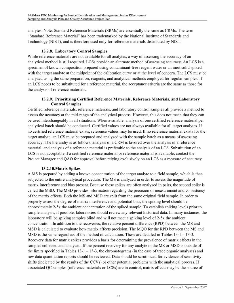
BASMAA POC Monitoring for Source Identification and Management Action Effectiveness Sampling and Analysis Plan and Quality Assurance Project Plan
Version 2, September 2017
47
analytes. Note: Standard Reference Materials (SRMs) are essentially the same as CRMs. The term
“Standard Reference Material” has been trademarked by the National Institute of Standards and
Technology (NIST), and is therefore used only for reference materials distributed by NIST.
13.2.8. Laboratory Control Samples
While reference materials are not available for all analytes, a way of assessing the accuracy of an
analytical method is still required. LCSs provide an alternate method of assessing accuracy. An LCS is a
specimen of known composition prepared using contaminant-free reagent water or an inert solid spiked
with the target analyte at the midpoint of the calibration curve or at the level of concern. The LCS must be
analyzed using the same preparation, reagents, and analytical methods employed for regular samples. If
an LCS needs to be substituted for a reference material, the acceptance criteria are the same as those for
the analysis of reference materials..
13.2.9. Prioritizing Certified Reference Materials, Reference Materials, and Laboratory
Control Samples
Certified reference materials, reference materials, and laboratory control samples all provide a method to
assess the accuracy at the mid-range of the analytical process. However, this does not mean that they can
be used interchangeably in all situations. When available, analysis of one certified reference material per
analytical batch should be conducted. Certified values are not always available for all target analytes. If
no certified reference material exists, reference values may be used. If no reference material exists for the
target analyte, an LCS must be prepared and analyzed with the sample batch as a means of assessing
accuracy. The hierarchy is as follows: analysis of a CRM is favored over the analysis of a reference
material, and analysis of a reference material is preferable to the analysis of an LCS. Substitution of an
LCS is not acceptable if a certified reference material or reference material is available, contact the
Project Manager and QAO for approval before relying exclusively on an LCS as a measure of accuracy.
13.2.10. Matrix Spikes
A MS is prepared by adding a known concentration of the target analyte to a field sample, which is then
subjected to the entire analytical procedure. The MS is analyzed in order to assess the magnitude of
matrix interference and bias present. Because these spikes are often analyzed in pairs, the second spike is
called the MSD. The MSD provides information regarding the precision of measurement and consistency
of the matrix effects. Both the MS and MSD are split from the same original field sample. In order to
properly assess the degree of matrix interference and potential bias, the spiking level should be
approximately 2-5x the ambient concentration of the spiked sample. To establish spiking levels prior to
sample analysis, if possible, laboratories should review any relevant historical data. In many instances, the
laboratory will be spiking samples blind and will not meet a spiking level of 2-5x the ambient
concentration. In addition to the recoveries, the relative percent difference (RPD) between the MS and
MSD is calculated to evaluate how matrix affects precision. The MQO for the RPD between the MS and
MSD is the same regardless of the method of calculation. These are detailed in Tables 13-1 – 13-3.
Recovery data for matrix spikes provides a basis for determining the prevalence of matrix effects in the
samples collected and analyzed. If the percent recovery for any analyte in the MS or MSD is outside of
the limits specified in Tables 13-1 – 13-3, the chromatograms (in the case of trace organic analyses) and
raw data quantitation reports should be reviewed. Data should be scrutinized for evidence of sensitivity
shifts (indicated by the results of the CCVs) or other potential problems with the analytical process. If
associated QC samples (reference materials or LCSs) are in control, matrix effects may be the source of
BASMAA POC Monitoring for Source Identification and Management Action Effectiveness Sampling and Analysis Plan and Quality Assurance Project Plan
Version 2, September 2017
48
the problem. If the standard used to spike the samples is different from the standard used to calibrate the
instrument, it must be checked for accuracy prior to attributing poor recoveries to matrix effects.
13.2.11. Laboratory Duplicates
In order to evaluate the precision of an analytical process, a field sample is selected and prepared in
duplicate. Specific requirements pertaining to the analysis of laboratory duplicates vary depending on the
type of analysis. The acceptance criteria for laboratory duplicates are specified in Tables 13-1 – 13-3.
13.2.12. Laboratory Duplicates vs. Matrix Spike Duplicates
Although the laboratory duplicate and matrix spike duplicate both provide information regarding
precision, they are unique measurements. Laboratory duplicates provide information regarding the
precision of laboratory procedures at actual ambient concentrations. The matrix spike duplicate provides
information regarding how the matrix of the sample affects both the precision and bias associated with the
results. It also determines whether or not the matrix affects the results in a reproducible manner.
MS/MSDs are often spiked at levels well above ambient concentrations, so thus are not representative of
typical sample precision. Because the two concepts cannot be used interchangeably, it is unacceptable to
analyze only an MS/MSD when a laboratory duplicate is required.
13.2.13. Replicate Analyses
The Monitoring Program will adopt the same terminology as SWAMP in defining replicate samples,
wherein replicate analyses are distinguished from duplicate analyses based simply on the number of
involved analyses. Duplicate analyses refer to two sample preparations, while replicate analyses refer to
three or more. Analysis of replicate samples is not explicitly required.
13.2.14. Surrogates
Surrogate compounds accompany organic measurements in order to estimate target analyte losses or
matrix effects during sample extraction and analysis. The selected surrogate compounds behave similarly
to the target analytes, and therefore any loss of the surrogate compound during preparation and analysis is
presumed to coincide with a similar loss of the target analyte. Surrogate compounds must be added to
field and QC samples prior to extraction, or according to the utilized method or SOP. Surrogate recovery
data are to be carefully monitored. If possible, isotopically labeled analogs of the analytes are to be used
as surrogates.
13.2.15. Internal Standards
To optimize gas chromatography mass spectrometry (GC-MS) analysis, internal standards (also referred
to as “injection internal standards”) may be added to field and QC sample extracts prior to injection. Use
of internal standards is particularly important for analysis of complex extracts subject to retention time
shifts relative to the analysis of standards. The internal standards can also be used to detect and correct for
problems in the GC injection port or other parts of the instrument. The analyst must monitor internal
standard retention times and recoveries to determine if instrument maintenance or repair or changes in
analytical procedures are indicated. Corrective action is initiated based on the judgment of the analyst.
Instrument problems that affect the data or result in reanalysis must be documented properly in logbooks
and internal data reports, and used by the laboratory personnel to take appropriate corrective action.
Performance criteria for internal standards are established by the method or laboratory SOP.
BASMAA POC Monitoring for Source Identification and Management Action Effectiveness Sampling and Analysis Plan and Quality Assurance Project Plan
Version 2, September 2017
49
13.2.16. Dual-Column Confirmation
Due to the high probability of false positives from single-column analyses, dual column confirmation
should be applied to all gas chromatography and liquid chromatography methods that do not provide
definitive identifications. It should not be restricted to instruments with electron capture detection (ECD).
13.2.17. Dilution of Samples
Final reported results must be corrected for dilution carried out during the process of analysis. In order to
evaluate the QC analyses associated with an analytical batch, corresponding batch QC samples must be
analyzed at the same dilution factor. For example, the results used to calculate the results of matrix spikes
must be derived from results for the native sample, matrix spike, and matrix spike duplicate analyzed at
the same dilution. Results derived from samples analyzed at different dilution factors must not be used to
calculate QC results.
13.2.18. Laboratory Corrective Action
Failures in laboratory measurement systems include, but are not limited to: instrument malfunction,
calibration failure, sample container breakage, contamination, and QC sample failure. If the failure can be
corrected, the analyst must document it and its associated corrective actions in the laboratory record and
complete the analysis. If the failure is not resolved, it is conveyed to the respective supervisor who should
determine if the analytical failure compromised associated results. The nature and disposition of the
problem must be documented in the data report that is sent to the Consultant-PM. Suggested ccorrective
actions are detailed in Table 13-9.
BASMAA POC Monitoring for Source Identification and Management Action Effectiveness Sampling and Analysis Plan and Quality Assurance Project Plan
Version 2, September 2017
50
Table 13-1. Measurement Quality Objectives - PCBs.
Laboratory Quality Control
Frequency of Analysis Measurement Quality Objective
Tuning2 Per analytical method Per analytical method
Calibration Initial method setup or when the calibration verification fails
Correlation coefficient (r2 >0.990) for linear and non-linear curves
If RSD<15%, average RF may be used to quantitate; otherwise use equation of the curve
First- or second-order curves only (not forced through the origin)
Refer to SW-846 methods for SPCC and CCC criteria2
Minimum of 5 points per curve (one of them at or below the RL)
Calibration Verification Per 12 hours
Expected response or expected concentration ±20%
RF for SPCCs=initial calibration4
Laboratory Blank Per 20 samples or per analytical batch, whichever is more frequent
<RL for target analytes
Reference Material Per 20 samples or per analytical batch
70-130% recovery if certified; otherwise, 50-150% recovery
Matrix Spike Per 20 samples or per analytical batch, whichever is more frequent
50-150% or based on historical laboratory control limits (average±3SD)
Matrix Spike Duplicate Per 20 samples or per analytical batch, whichever is more frequent
50-150% or based on historical laboratory control limits (average±3SD); RPD<25%
Surrogate Included in all samples and all QC samples
Based on historical laboratory control limits (50-150% or better)
Internal Standard Included in all samples and all QC samples (as available)
Per laboratory procedure
Field Quality Control Frequency of Analysis Measurement Quality Objective
Field Duplicate 5% of total Project sample count (sediment and water samples only)
RPD<25% (n/a if concentration of either sample<RL)
Field Blank Not required for the Monitoring Program
<RL for target analytes

BASMAA POC Monitoring for Source Identification and Management Action Effectiveness Sampling and Analysis Plan and Quality Assurance Project Plan
Version 2, September 2017
51
Table 13-2. Measurement Quality Objectives – Inorganic Analytes.
Laboratory Quality Control
Frequency of Analysis Measurement Quality Objective
Calibration Standard Per analytical method or manufacturer’s specifications
Per analytical method or manufacturer’s specifications
Continuing Calibration Verification
Per 10 analytical runs 80-120% recovery
Laboratory Blank Per 20 samples or per analytical batch, whichever is more frequent
<RL for target analyte
Reference Material Per 20 samples or per analytical batch, whichever is more frequent
75-125% recovery
Matrix Spike Per 20 samples or per analytical batch, whichever is more frequent
75-125% recovery
Matrix Spike Duplicate Per 20 samples or per analytical batch, whichever is more frequent
75-125% recovery ; RPD<25%
Laboratory Duplicate Per 20 samples or per analytical batch, whichever is more frequent
RPD<25% (n/a if concentration of either sample<RL)
Internal Standard Accompanying every analytical run when method appropriate
60-125% recovery
Field Quality Control Frequency of Analysis Measurement Quality Objective
Field Duplicate 5% of total Project sample count RPD<25% (n/a if concentration of either sample<RL), unless
otherwise specified by method
Field Blank, Equipment Field, Eqpt Blanks
Not required for the Monitoring Program Blanks<RL for target analyte
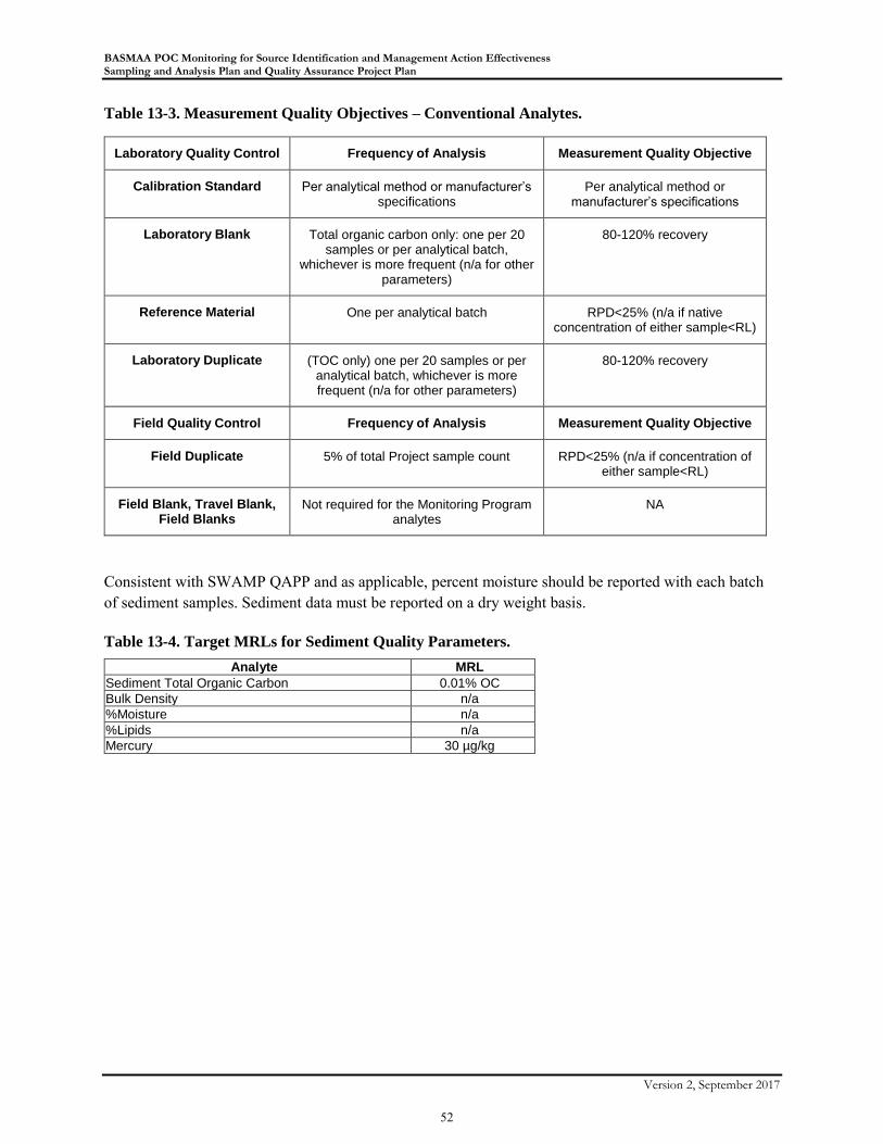
BASMAA POC Monitoring for Source Identification and Management Action Effectiveness Sampling and Analysis Plan and Quality Assurance Project Plan
Version 2, September 2017
52
Table 13-3. Measurement Quality Objectives – Conventional Analytes.
Laboratory Quality Control Frequency of Analysis Measurement Quality Objective
Calibration Standard Per analytical method or manufacturer’s specifications
Per analytical method or manufacturer’s specifications
Laboratory Blank Total organic carbon only: one per 20 samples or per analytical batch,
whichever is more frequent (n/a for other parameters)
80-120% recovery
Reference Material One per analytical batch RPD<25% (n/a if native concentration of either sample<RL)
Laboratory Duplicate (TOC only) one per 20 samples or per analytical batch, whichever is more frequent (n/a for other parameters)
80-120% recovery
Field Quality Control Frequency of Analysis Measurement Quality Objective
Field Duplicate 5% of total Project sample count RPD<25% (n/a if concentration of either sample<RL)
Field Blank, Travel Blank, Field Blanks
Not required for the Monitoring Program analytes
NA
Consistent with SWAMP QAPP and as applicable, percent moisture should be reported with each batch
of sediment samples. Sediment data must be reported on a dry weight basis.
Table 13-4. Target MRLs for Sediment Quality Parameters.
Analyte MRL
Sediment Total Organic Carbon 0.01% OC
Bulk Density n/a
%Moisture n/a
%Lipids n/a
Mercury 30 µg/kg
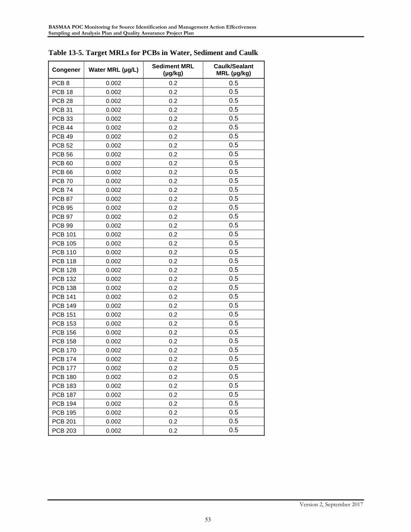
BASMAA POC Monitoring for Source Identification and Management Action Effectiveness Sampling and Analysis Plan and Quality Assurance Project Plan
Version 2, September 2017
53
Table 13-5. Target MRLs for PCBs in Water, Sediment and Caulk
Congener Water MRL (µg/L) Sediment MRL
(µg/kg) Caulk/Sealant MRL (µg/kg)
PCB 8 0.002 0.2 0.5
PCB 18 0.002 0.2 0.5
PCB 28 0.002 0.2 0.5
PCB 31 0.002 0.2 0.5
PCB 33 0.002 0.2 0.5
PCB 44 0.002 0.2 0.5
PCB 49 0.002 0.2 0.5
PCB 52 0.002 0.2 0.5
PCB 56 0.002 0.2 0.5
PCB 60 0.002 0.2 0.5
PCB 66 0.002 0.2 0.5
PCB 70 0.002 0.2 0.5
PCB 74 0.002 0.2 0.5
PCB 87 0.002 0.2 0.5
PCB 95 0.002 0.2 0.5
PCB 97 0.002 0.2 0.5
PCB 99 0.002 0.2 0.5
PCB 101 0.002 0.2 0.5
PCB 105 0.002 0.2 0.5
PCB 110 0.002 0.2 0.5
PCB 118 0.002 0.2 0.5
PCB 128 0.002 0.2 0.5
PCB 132 0.002 0.2 0.5
PCB 138 0.002 0.2 0.5
PCB 141 0.002 0.2 0.5
PCB 149 0.002 0.2 0.5
PCB 151 0.002 0.2 0.5
PCB 153 0.002 0.2 0.5
PCB 156 0.002 0.2 0.5
PCB 158 0.002 0.2 0.5
PCB 170 0.002 0.2 0.5
PCB 174 0.002 0.2 0.5
PCB 177 0.002 0.2 0.5
PCB 180 0.002 0.2 0.5
PCB 183 0.002 0.2 0.5
PCB 187 0.002 0.2 0.5
PCB 194 0.002 0.2 0.5
PCB 195 0.002 0.2 0.5
PCB 201 0.002 0.2 0.5
PCB 203 0.002 0.2 0.5

BASMAA POC Monitoring for Source Identification and Management Action Effectiveness Sampling and Analysis Plan and Quality Assurance Project Plan
Version 2, September 2017
54
Table 13-6. Size Distribution Categories for Grain Size in Sediment
Wentworth Size Category Size MRL
Clay <0.0039 mm 1%
Silt 0.0039 mm to <0.0625 mm 1%
Sand, very fine 0.0625 mm to <0.125 mm 1%
Sand, fine 0.125 mm to <0.250 mm 1%
Sand, medium 0.250 mm to <0.5 mm 1%
Sand, coarse 0.5 mm to < 1.0 mm 1%
Sand, very coarse 1.0 mm to < 2 mm 1%
Gravel 2 mm and larger 1%
Table 13-7. Target MRLs for TOC, SSC, and Mercury in Water
Analyte MRL
Total Organic Carbon 0.6 mg/L
Suspended Sediment Concentration 0.5 mg/L
Mercury 0.0002 µg/L

BASMAA POC Monitoring for Source Identification and Management Action Effectiveness Sampling and Analysis Plan and Quality Assurance Project Plan
Version 2, September 2017
55
Table 13-8. Corrective Action – Laboratory and Field Quality Control
Laboratory
Quality Control
Recommended Corrective Action
Calibration Recalibrate the instrument. Affected samples and associated quality control must be
reanalyzed following successful instrument recalibration.
Calibration
Verification
Reanalyze the calibration verification to confirm the result. If the problem continues, halt
analysis and investigate the source of the instrument drift. The analyst should determine if the
instrument must be recalibrated before the analysis can continue. All of the samples not
bracketed by acceptable calibration verification must be reanalyzed.
Laboratory Blank Reanalyze the blank to confirm the result. Investigate the source of contamination. If the source
of the contamination is isolated to the sample preparation, the entire batch of samples, along
with the new laboratory blanks and associated QC samples, should be prepared and/or re-
extracted and analyzed. If the source of contamination is isolated to the analysis procedures,
reanalyze the entire batch of samples. If reanalysis is not possible, the associated sample
results must be flagged to indicate the potential presence of the contamination.
Reference
Material
Reanalyze the reference material to confirm the result. Compare this to the matrix spike/matrix
spike duplicate recovery data. If adverse trends are noted, reprocess all of the samples
associated with the batch.
Matrix Spike The spiking level should be near the midrange of the calibration curve or at a level that does
not require sample dilution. Reanalyze the matrix spike to confirm the result. Review the
recovery obtained for the matrix spike duplicate. Review the results of the other QC samples
(such as reference materials) to determine if other analytical problems are a potential source of
the poor spike recovery.
Matrix Spike
Duplicate
The spiking level should be near the midrange of the calibration curve or at a level that does
not require sample dilution. Reanalyze the matrix spike duplicate to confirm the result. Review
the recovery obtained for the matrix spike. Review the results of the other QC samples (such as
reference materials) to determine if other analytical problems are a potential source of the poor
spike recovery.
Internal Standard Check the response of the internal standards. If the instrument continues to generate poor
results, terminate the analytical run and investigate the cause of the instrument drift.
Surrogate Analyze as appropriate for the utilized method. Troubleshoot as needed. If no instrument
problem is found, samples should be re-extracted and reanalyzed if possible.
Field Quality
Control
Recommended Corrective Action
Field Duplicate Visually inspect the samples to determine if a high RPD between results could be attributed to
sample heterogeneity. For duplicate results due to matrix heterogeneity, or where ambient
concentrations are below the reporting limit, qualify the results and document the
heterogeneity. All failures should be communicated to the project coordinator, who in turn will
follow the process detailed in the method.
Field Blank Investigate the source of contamination. Potential sources of contamination include sampling
equipment, protocols, and handling. The laboratory should report evidence of field
contamination as soon as possible so corrective actions can be implemented. Samples
collected in the presence of field contamination should be flagged.

BASMAA POC Monitoring for Source Identification and Management Action Effectiveness Sampling and Analysis Plan and Quality Assurance Project Plan
Version 2, September 2017
56
14. Inspection/Acceptance for Supplies and Consumables Each sampling event conducted for the Monitoring Program will require use of appropriate consumables
to reduce likelihood of sample contamination. The Field-PM will be responsible for ensuring that all
supplies are appropriate prior to their use. Inspection requirements for sampling consumables and supplies
are summarized in Table 14-1.
Table 14-1. Inspection / Acceptance Testing Requirements for Consumables and Supplies
Project-
related
Supplies
Inspection /
Testing
Specifications
Acceptance Criteria Frequency Responsible Person
Sampling
Containers
Sampling
supplies
Visual Appropriateness; no
evident contamination or
damage; within expiration
date
Each purchase Field Crew Leader
15. Non Direct Measurements, Existing Data No data from external sources are planned to be used with this project.
16. Data Management As previously discussed, the Monitoring Program data management will conform to protocols dictated by
the study designs (BASMAA 2017a, b). A summary of specific data management aspects is provided
below.
16.1. Field Data Management
All field data will be reviewed for legibility and errors as soon as possible after the conclusion of
sampling. All field data that is entered electronically will be hand-checked at a rate of 10% of entries as a
check on data entry. Any corrective actions required will be documented in correspondence to the QA
Officer.
16.2. Laboratory Data Management
Record keeping of laboratory analytical data for the proposed project will employ standard record-
keeping and tracking practices. All laboratory analytical data will be entered into electronic files by the
instrumentation being used or, if data is manually recorded, then it will be entered by the analyst in charge
of the analyses, per laboratory standard procedures.
Following the completion of internal laboratory quality control checks, analytical results will be
forwarded electronically to the Field-PM. The analytical laboratories will provide data in electronic
format, encompassing both a narrative and electronic data deliverable (EDD).

BASMAA POC Monitoring for Source Identification and Management Action Effectiveness Sampling and Analysis Plan and Quality Assurance Project Plan
Version 2, September 2017
57
17. Assessments and Response Actions
17.1. Readiness Reviews
The Field-PM will review all field equipment, instruments, containers, and paperwork to ensure that
everything is ready prior to each sampling event. All sampling personnel will be given a brief review of
the goals and objectives of the sampling event and the sampling procedures and equipment that will be
used to achieve them. It is important that all field equipment be clean and ready to use when it is needed.
Therefore, prior to using all sampling and/or field measurement equipment, each piece of equipment will
be checked to make sure that it is in proper working order. Equipment maintenance records will be
checked to ensure that all field instruments have been properly maintained and that they are ready for use.
Adequate supplies of all preservatives, bottles, labels, waterproof pens, etc. will be checked before each
field event to make sure that there are sufficient supplies to successfully support each sampling event,
and, as applicable, are within their expiration dates. It is important to make sure that all field activities and
measurements are properly recorded in the field. Therefore, prior to starting each field event, necessary
paperwork such as logbooks, chain of custody record forms, etc. will be checked to ensure that sufficient
amounts are available during the field event. In the event that a problem is discovered during a readiness
review it will be noted in the field log book and corrected before the field crew is deployed. The actions
taken to correct the problem will also be documented with the problem in the field log book. This
information will be communicated by the Field-PM prior to conducting relevant sampling. The Field-PM
will track corrective actions taken.
17.2. Post Sampling Event Reviews
The Field-PM will be responsible for post sampling event reviews. Any problems that are noted will be
documented along with recommendations for correcting the problem. Post sampling event reviews will be
conducted following each sampling event in order to ensure that all information is complete and any
deviations from planned methodologies are documented. Post sampling event reviews will include field
sampling activities and field measurement documentation in order to help ensure that all information is
complete. The reports for each post sampling event will be used to identify areas that may be improved
prior to the next sampling event.
17.3. Laboratory Data Reviews
The Field-PM will be responsible for reviewing the laboratory's data for completeness and accuracy. The
data will also be checked to make sure that the appropriate methods were used and that all required QC
data was provided with the sample analytical results. Any laboratory data that is discovered to be
incorrect or missing will immediately be reported to the both the laboratory and Consultant-PM. The
laboratory's QA manual details the procedures that will be followed by laboratory personnel to correct
any invalid or missing data. The Consultant-PM has the authority to request re-testing if a review of any
of the laboratory data is found to be invalid or if it would compromise the quality of the data and resulting
conclusions from the proposed project.
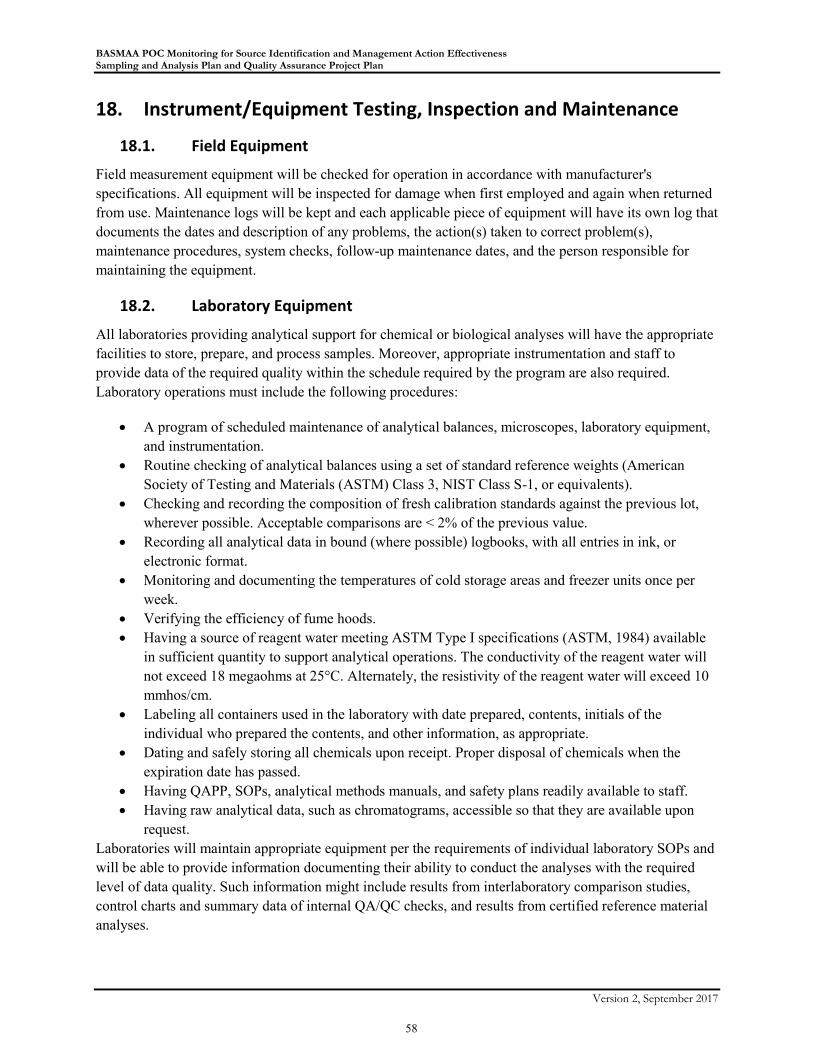
BASMAA POC Monitoring for Source Identification and Management Action Effectiveness Sampling and Analysis Plan and Quality Assurance Project Plan
Version 2, September 2017
58
18. Instrument/Equipment Testing, Inspection and Maintenance
18.1. Field Equipment
Field measurement equipment will be checked for operation in accordance with manufacturer's
specifications. All equipment will be inspected for damage when first employed and again when returned
from use. Maintenance logs will be kept and each applicable piece of equipment will have its own log that
documents the dates and description of any problems, the action(s) taken to correct problem(s),
maintenance procedures, system checks, follow-up maintenance dates, and the person responsible for
maintaining the equipment.
18.2. Laboratory Equipment
All laboratories providing analytical support for chemical or biological analyses will have the appropriate
facilities to store, prepare, and process samples. Moreover, appropriate instrumentation and staff to
provide data of the required quality within the schedule required by the program are also required.
Laboratory operations must include the following procedures:
A program of scheduled maintenance of analytical balances, microscopes, laboratory equipment,
and instrumentation.
Routine checking of analytical balances using a set of standard reference weights (American
Society of Testing and Materials (ASTM) Class 3, NIST Class S-1, or equivalents).
Checking and recording the composition of fresh calibration standards against the previous lot,
wherever possible. Acceptable comparisons are < 2% of the previous value.
Recording all analytical data in bound (where possible) logbooks, with all entries in ink, or
electronic format.
Monitoring and documenting the temperatures of cold storage areas and freezer units once per
week.
Verifying the efficiency of fume hoods.
Having a source of reagent water meeting ASTM Type I specifications (ASTM, 1984) available
in sufficient quantity to support analytical operations. The conductivity of the reagent water will
not exceed 18 megaohms at 25°C. Alternately, the resistivity of the reagent water will exceed 10
mmhos/cm.
Labeling all containers used in the laboratory with date prepared, contents, initials of the
individual who prepared the contents, and other information, as appropriate.
Dating and safely storing all chemicals upon receipt. Proper disposal of chemicals when the
expiration date has passed.
Having QAPP, SOPs, analytical methods manuals, and safety plans readily available to staff.
Having raw analytical data, such as chromatograms, accessible so that they are available upon
request.
Laboratories will maintain appropriate equipment per the requirements of individual laboratory SOPs and
will be able to provide information documenting their ability to conduct the analyses with the required
level of data quality. Such information might include results from interlaboratory comparison studies,
control charts and summary data of internal QA/QC checks, and results from certified reference material
analyses.
BASMAA POC Monitoring for Source Identification and Management Action Effectiveness Sampling and Analysis Plan and Quality Assurance Project Plan
Version 2, September 2017
59
19. Instrument/Equipment Calibration and Frequency
19.1. Field Measurements
Any equipment used should be visually inspected during mobilization to identify problems that would
result in loss of data. As appropriate, equipment-specific SOPs should be consulted for equipment
calibration.
19.2. Laboratory Analyses
19.2.1. In-house Analysis – XRF Screening
A portable XRF analyzer will be used as a screening tool to estimate the chlorine concentration in each
caulk sample. Since caulk often contains in excess of 1% PCBs and detection limits of portable XRF may
be in the ppm range, the portable XRF may be able to detect chlorine within caulk containing PCBs down
to about 0.1%. The analysis will be performed on the field samples using a test stand. The analyzer will
be calibrated for chlorine using plastic pellet European reference materials (EC680 and EC681) upon first
use, and standardized each time the instrument is turned on and prior to any caulk Cl analysis. The
standardization procedure will entail a calibration analysis of the materials provided/recommended with
the XRF analyzer. Analyses will be conducted in duplicate on each sample and notes kept. The mean will
be used for comparison to GC–MS results.
19.2.2. Contract Laboratory Analyses
The procedures for and frequency of calibration will vary depending on the chemical parameters being
determined. Equipment is maintained and checked according to the standard procedures specified in each
laboratory’s instrument operation instruction manual.
Upon initiation of an analytical run, after each major equipment disruption, and whenever on-going
calibration checks do not meet recommended DQOs (see Section 13), analytical systems will be
calibrated with a full range of analytical standards. Immediately after this procedure, the initial calibration
must be verified through the analysis of a standard obtained from a different source than the standards
used to calibrate the instrumentation and prepared in an independent manner and ideally having certified
concentrations of target analytes of a CRM or certified solution. Frequently, calibration standards are
included as part of an analytical run, interspersed with actual samples.
Calibration curves will be established for each analyte and batch analysis from a calibration blank and a
minimum of three analytical standards of increasing concentration, covering the range of expected sample
concentrations. Only those data resulting from quantification within the demonstrated working calibration
range may be reported by the laboratory.
The calibration standards will be prepared from reference materials available from the EPA repository, or
from available commercial sources. The source, lot number, identification, and purity of each reference
material will be recorded. Neat compounds will be prepared weight/volume using a calibrated analytical
balance and Class A volumetric flasks. Reference solutions will be diluted using Class A volumetric
glassware. Individual stock standards for each analyte will be prepared. Combination working standards
will be prepared by volumetric dilution of the stock standards. The calibration standards will be stored at -
20º C. Newly prepared standards will be compared with existing standards prior to their use. All solvents
BASMAA POC Monitoring for Source Identification and Management Action Effectiveness Sampling and Analysis Plan and Quality Assurance Project Plan
Version 2, September 2017
60
used will be commercially available, distilled in glass, and judged suitable for analysis of selected
chemicals. Stock standards and intermediate standards are prepared on an annual basis and working
standards are prepared every three months.
Sampling and analytical logbooks will be kept to record inspections, calibrations, standard identification
numbers, the results of calibrations, and corrective action taken. Equipment logs will document
instrument usage, maintenance, repair and performance checks. Daily calibration data will be stored with
the raw sample data
20. Data Review, Verification, and Validation Defining data review, verification, and validation procedures helps to ensure that Monitoring Plan data
will be reviewed in an objective and consistent manner. Data review is the in-house examination to ensure
that the data have been recorded, transmitted, and processed correctly. The Field-PM will be responsible
for initial data review for field forms and field measurements; QA Officer will be responsible for doing so
for data reported by analytical laboratories. This includes checking that all technical criteria have been
met, documenting any problems that are observed and, if possible, ensuring that deficiencies noted in the
data are corrected.
In-house examination of the data produced from the proposed Monitoring Program will be conducted to
check for typical types of errors. This includes checking to make sure that the data have been recorded,
transmitted, and processed correctly. The kinds of checks that will be made will include checking for data
entry errors, transcription errors, transformation errors, calculation errors, and errors of data omission.
Data generated by Program activities will be reviewed against MQOs that were developed and
documented in Section 13. This will ensure that the data will be of acceptable quality and that it will be
SWAMP-comparable with respect to minimum expected MQOs.
QA/QC requirements were developed and documented in Sections 13.1 and 13.2, and the data will be
checked against this information. Checks will include evaluation of field and laboratory duplicate results,
field and laboratory blank data, matrix spike recovery data, and laboratory control sample data pertinent
to each method and analytical data set. This will ensure that the data will be SWAMP-comparable with
respect to quality assurance and quality control procedures.
Field data consists of all information obtained during sample collection and field measurements, including
that documented in field log books and/or recording equipment, photographs, and chain of custody forms.
Checks of field data will be made to ensure that it is complete, consistent, and meets the data management
requirements that were developed and documented in Section 13.1.
Lab data consists of all information obtained during sample analysis. Initial review of laboratory data will
be performed by the laboratory QA/QC Officer in accordance with the lab's internal data review
procedures. However, upon receipt of laboratory data, the Lab-PM will perform independent checks to
ensure that it is complete, consistent, and meets the data management requirements that were developed
and documented in Section 13.2. This review will include evaluation of field and laboratory QC data and
also making sure that the data are reported in compliance with procedures developed and documented in
Section 7.

BASMAA POC Monitoring for Source Identification and Management Action Effectiveness Sampling and Analysis Plan and Quality Assurance Project Plan
Version 2, September 2017
61
Data verification is the process of evaluating the completeness, correctness, and conformance /
compliance of a specific data set against the method, procedural, or contractual specifications. The Lab-
PM and Data Manager will conduct data verification, as described in Section 13 on Quality Control, in
order to ensure that it is SWAMP-comparable with respect to completeness, correctness, and
conformance with minimum requirements.
Data will be separated into three categories for use with making decisions based upon it. These categories
are: (1) data that meets all acceptance requirements, (2) data that has been determined to be unacceptable
for use, and (3) data that may be conditionally used and that is flagged as per US EPA specifications.
21. Verification and Validation Methods Defining the methods for data verification and validation helps to ensure that Program data are evaluated
objectively and consistently. For the proposed Program many of these methods have been described in
Section 20. Additional information is provided below.
All data records for the Monitoring Program will be checked visually and will be recorded as checked by
the checker's initials as well as with the dates on which the records were checked. Consultant Team staff
will perform an independent re-check of at least 10% of these records as the validation methodology.
All of the laboratory's data will be checked as part of the verification methodology process. Each contract
laboratory's Project Analyst will conduct reviews of all laboratory data for verification of their accuracy.
Any data that is discovered to be incorrect or missing during the verification or validation process will
immediately be reported to the Consultant-PM. If errors involve laboratory data then this information will
also be reported to the laboratory's QA Officer. Each laboratory's QA manual details the procedures that
will be followed by laboratory personnel to correct any invalid or missing data. The laboratory’s QA
Officer will be responsible for reporting and correcting any errors that are found in the data during the
verification and validation process.
If there are any data quality problems identified, the QA Officer will try to identify whether the problem
is a result of project design issues, sampling issues, analytical methodology issues, or QA/QC issues
(from laboratory or non-laboratory sources). If the source of the problems can be traced to one or more of
these basic activities then the person or people in charge of the areas where the issues lie will be contacted
and efforts will be made to immediately resolve the problem. If the issues are too broad or severe to be
easily corrected then the appropriate people involved will be assembled to discuss and try to resolve the
issue(s) as a group. The QA Officer has the final authority to resolve any issues that may be identified
during the verification and validation process.
22. Reconciliation with User Requirements The purpose of the Monitoring Program is to comply with Provisions of the MRP and provide data that
can be used to identify sources of PCBs to urban runoff, and to evaluate management action effectiveness
in removing POCs from urban runoff in the Bay Area. The objectives of the Monitoring Program are to
provide the following outcomes:
1. Satisfy MRP Provision C.8.f. requirements for POC monitoring for source identification;
BASMAA POC Monitoring for Source Identification and Management Action Effectiveness Sampling and Analysis Plan and Quality Assurance Project Plan
Version 2, September 2017
62
2. Satisfy MRP Provision C.12.e.ii requirements to evaluate PCBs presence in caulks/sealants used
in storm drain or roadway infrastructure in public ROWs;
3. Report the range of PCB concentrations observed in 20 composite samples of caulk/sealant
collected from structures installed or rehabilitated during the 1970’s;
4. Satisfy MRP Provision C.8.f. requirements for POC monitoring for management action
effectiveness;
5. Quantify the annual mass of mercury and PCBs captured in HDS Unit sumps during
maintenance; and
6. Identify BSM mixtures for future field testing that provide the most effective mercury and PCBs
treatment in laboratory column tests.
Information from field data reports (including field activities, post sampling events, and corrective
actions), laboratory data reviews (including errors involving data entry, transcriptions, omissions, and
calculations and laboratory audit reports), reviews of data versus MQOs, reviews against QA/QC
requirements, data verification reports, data validation reports, independent data checking reports, and
error handling reports will be used to determine whether or not the Monitoring Program's objectives have
been met. Descriptions of the data will be made with no extrapolation to more general cases.
Data from all monitoring measurements will be summarized in tables. Additional data may also be
represented graphically when it is deemed helpful for interpretation purposes.
The above evaluations will provide a comprehensive assessment of how well the Program meets its
objectives. The final project reports will reconcile results with project MQOs.
23. References California Regional Water Quality Control Board, San Francisco Bay Region. Municipal Regional
Stormwater NPDES Permit Order R2-2015-0049 NPDES Permit No. CAS612008. November 19, 2015.
BASMAA. 2016. BASMAA Regional Monitoring Coalition Creek Status and Toxicity and Pesticide
Monitoring Standard Operating Procedures. Prepared for Bay Area Stormwater Management Agencies
Association. Version 3, March 2016.
BASMAA 2017a. The Evaluation of PCBs Presence in Public Roadway and Storm Drain Infrastructure
Caulk and Sealants Study Design. Prepared by EOA Inc. and the San Francisco Estuary Institute (SFEI).
June 2017.
BASMAA 2017b. POC Monitoring for Management Action Effectiveness Study Design. Prepared by the
Office of Water Programs, Sacramento State, CA, EOA Inc., and the San Francisco Estuary Institute
(SFEI). July 2017.
BASMAA, 2017c. Clean Watershed for a Clean Bay (CW4CB) Final Report. Prepared for Bay Area
Stormwater Management Agencies Association. Prepared by Geosyntec and EOA, Inc., May 2017.
Klosterhaus, S. McKee, L.J. Yee, D., Kass, J.M., and Wong, A. 2014. Polychlorinated Biphenyls in the
Exterior Caulk of San Francisco Bay Area Buildings, California, USA. Environment International 66, 38-
43.
Surface Water Ambient Monitoring Program Quality Assurance Team, 2013. SWAMP Quality Assurance
Project Plan. Prepared for the California State Water Quality Control Board. 2013.

BASMAA POC Monitoring for Source Identification and Management Action Effectiveness Sampling and Analysis Plan and Quality Assurance Project Plan
Version 2, September 2017
63
24. Appendix A: Field Documentation

64
Pg of Pgs
Storm Drain
Catch BasinSidewalk Bridge
Concrete Asphalt
Good Fair Poor
Hard/brittle
Surface Submerged Exposed
Composite ID: Contractor:
Date (mm/dd/yyyy):
ArrivalTime:
Photos (Y / N)
Caulk/Sealant Sampling Field Data Sheet
SITE/SAMPLING DESCRIPTION AND COMMENTS:
Other:
Sample ID:
DepartureTime:
Condition of Structure:
Structure Material:
Amount of Caulk/Sealant
observed on structure
Crack dimensions: Spacing of expansion joints
Other:
Other:
Year of Strucutre Construction
Year of Repair
Land-Use at the Sample Location: Open Space
Other:
Diagram of Structure (if needed) to identify where
caulk/sealants were located in/on structure
Description of Caulk or Sealant Sample Collected:
Description of Structure: (Do not include any information on the location of the structure)
Structure Type:Curb/GutterRoadway Surface
Industrial (pre-1980; post-1980)
Commercial (pre-1980; post 1980)
Residential (pre 1980; post 1980)
Failure Reason
Photo Log Identifier
Location Between Joints At street level Below street level Other:
caulk between adjoing surfaces of same material (e.g., concrete-concrete); Describe:
caulk between adjoining surfaces of different types of material (e.g., concrete-asphalt); Describe:
Other:
Crack Repair (describe):
Other:
Personnel:
Poor (crumbling/disintegrating) Other:
Length&width of caulk bead sampled: Other:
COLLECTION DEVICE:
Samples Taken
Equiptment type used:
Good (intact/whole)
Caulk
Application or Usage
Sealant
Color
Texture
Condition
Other:Soft/pliable
65
*GPS/DGPS
Target ( if known) :
*Actual:
Grain Size PCBs Hg Bulk Density TOC OTHER
SITE/SAMPLING DESCRIPTION AND COMMENTS:
Sample ID (City-
Catchment ID-Sample DepthCollec (cm) Composite / Grab (C / G)
SOILPOSITION Submerged, Exposed
Samples Taken ( 3 digit ID nos. of containers filled) Field Dup at Site? YES / N O: (create separate datasheet for FDs, with unique IDs (i.e., blind samples)
COLLECTION DEVICE: Equiptment type used: Scoop (SS / PC / PE), Core (SS / PC / PE), Grab (Van Veen / Eckman / Petite Ponar), Broom (nylon, natural f iber)
SOILODOR: None, Sulf ides, Sew age, Petroleum, Mixed, Other_______________
SOILCOLOR: Colorless, Green, Yellow , Brow n
SOILCOMPOSITION: Silt/Clay, Sand, Gravel, Cobble, Mixed, Debris
None,Sulf ides,Sew age,Petroleum,Smoke,Other_______
SKY CODE: Clear, Partly Cloudy, Overcast, Fog, Smoky, Hazy
PRECIP: None, Fog, Drizzle, Rain
PRECIP (last 24 hrs): Unknow n, <1", >1", None
GPS Device:
Estimate of Volume of Sediment in the HDS unit sump prior to cleanout:
Estimate of Volume of Sediment REMOVED from the HDS unit sump during the cleanout:
Env. Conditions WIND
DIRECTION
(from):
SITE ODOR:
Photos (Y / N) Lat (dd.ddddd) Long (ddd.ddddd) Address, Location, and Sketches (if needed)
Photo Log Identif ier
HDS Catchment ID: ArrivalTime: DepartureTime: *SampleTime (1st sample):Failure Reason
Personnel:
HDS Unit Sampling Field Data Sheet (Sediment Chemistry) Contractor: Pg of Pgs
City: Date (mm/dd/yyyy): / / *Contractor:
N
S
EW
66
*GPS/DGPS
Target:
*Actual:
None, Fog, Drizzle, Rain, Snow
None, Sulf ides, Sew age, Petroleum, Mixed, Other_______________
Carboy ID #
Collection
Depth (m)
PHOTOS (RB & LB assigned when facing
downstream; RENAM E to
StationCode_yyyy_mm_dd_uniquecode):
Sample Type (Grab=G;
Integrated = I)
Indiv bottle (by hand, by pole, by bucket); Teflon
tubing; Kemmer; Pole & Beaker; OtherField Dup (Yes/No)Start Sample Time End Sample Time
COMMENTS:
OBSERVED FLOW: NA, Dry Waterbody Bed, No Obs Flow , Isolated Pool, Trickle (<0.1cfs), 0.1-1cfs, 1-5cfs, 5-20cfs, 20-50cfs, 50-200cfs, >200cfs
Field Samples (Record Time Sample Collected)
WATERCOLOR: Colorless, Green, Yellow , Brow n 3: (RB / LB / BB / US / DS / ##)
OVERLAND RUNOFF (Last 24 hrs): none, light, moderate / heavy, unknow n
WATERCLARITY: Clear (see bottom), Cloudy (>4" vis), Murky (<4" vis) PRECIPITATION: 2: (RB / LB / BB / US / DS / ##)
WATERODOR: PRECIPITATION (last 24 hrs): Unknow n, <1", >1", None
OTHER PRESENCE: Vascular,Nonvascular,OilySheen,Foam,Trash,Other______ 1: (RB / LB / BB / US / DS / ##)
DOMINANT SUBSTRATE: Bedrock, Concrete, Cobble, Boulder, Gravel, Sand, Mud, Unk, Other_________
SITE ODOR: None,Sulf ides,Sew age,Petroleum,Smoke,Other_______
SKY CODE: Clear, Partly Cloudy, Overcast, Fog, Smoky, HazyWIND
DIRECTION
(from):
Datum: NAD83 Accuracy ( ft / m ): - Sampling Location (e.g., gutter at SW corner of 10th Street)
Habitat Observations (CollectionMethod = Habitat_generic ) WADEABILITY:
Y / N / Unk
BEAUFORT
SCALE (see
attachment)
Lat (dd.ddddd) Long (ddd.ddddd)
GPS Device: -OCCUPATION METHOD: Walk-in Bridge R/V __________ Other
Personnel: ArrivalTime: DepartureTime: *Protocol:
*PurposeFailure:
Stormwater Field Data Sheet (Water Chemistry) Entered in d-base (initial/date) Pg of Pgs
*Station Code: *Date (mm/dd/yyyy): / / *Agency:
N
S
EW

67
Stormwater Influent Samples – Office of Water Programs
Sample Receiving
Date (mm/dd/yy): Time
(24
hr) :
Team Member’s Initial:
Carboy Temperatur
e
pH Observations
1
2
3
4
5
6
7
68
Stormwater Column Tests – Office of Water Programs
Sampling Run
Date (mm/dd/yy): Time (24 hr) : Team Member’s Initials: Column ID:
During Test - Timed Measurements
Time Water Depth Media Condition Other Observations
Grab Sample - Beginning of Run
Time Water Depth Turbidity (NTU) Temp pH Other Observations
Grab Sample - Middle of Run
Time Water Depth Turbidity (NTU) Temp pH Other Observations
Grab Sample - End of Run
Time Water Depth Turbidity (NTU) Temp pH Other Observations
Grab Sample - Mercury
Time Water Depth Turbidity (NTU) Temp pH Other Observations

69
25. Appendix B: Laboratory Standard Operating Procedures (SOPs)

Final Project Report – POC Removal Effectiveness of HDS Units 2019
APPENDIX C: QA SUMMARY REPORTS
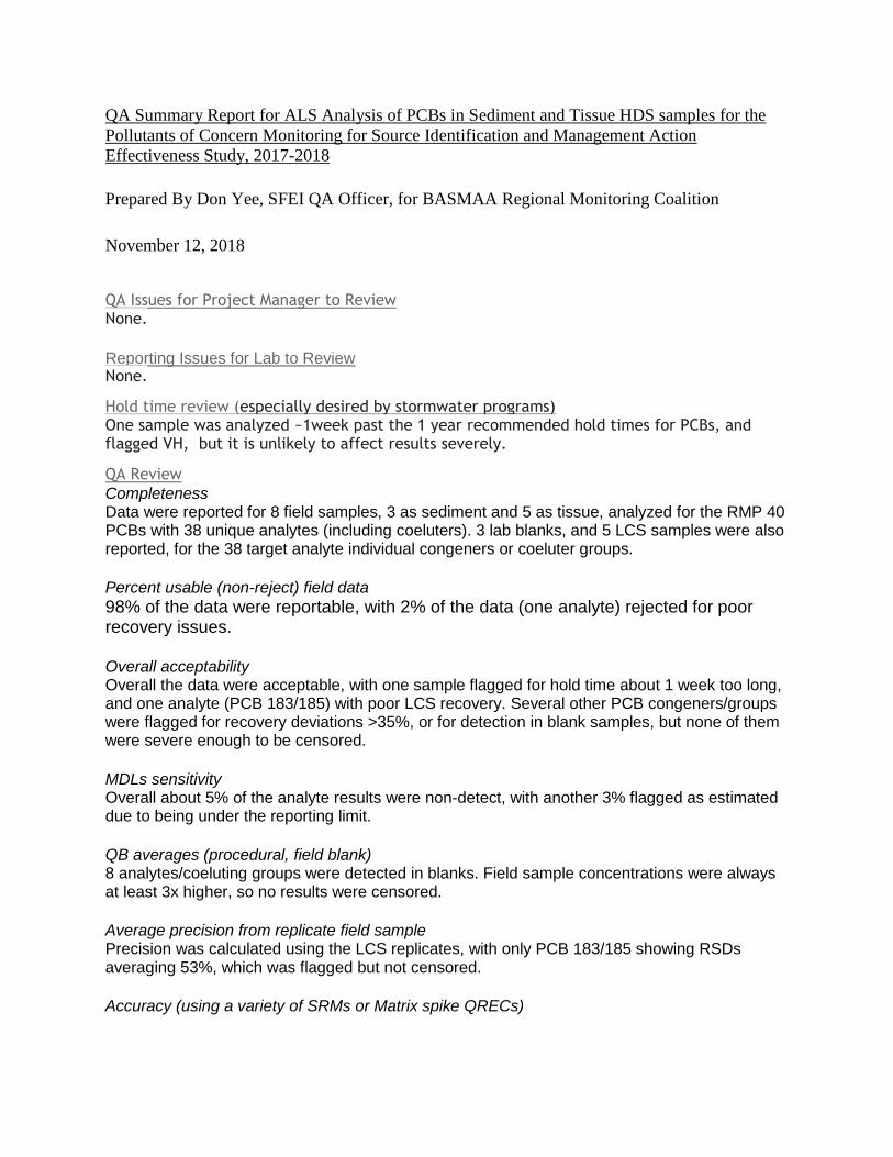
QA Summary Report for ALS Analysis of PCBs in Sediment and Tissue HDS samples for the
Pollutants of Concern Monitoring for Source Identification and Management Action
Effectiveness Study, 2017-2018
Prepared By Don Yee, SFEI QA Officer, for BASMAA Regional Monitoring Coalition
November 12, 2018
QA Issues for Project Manager to Review None.
Reporting Issues for Lab to Review None.
Hold time review (especially desired by stormwater programs) One sample was analyzed ~1week past the 1 year recommended hold times for PCBs, and flagged VH, but it is unlikely to affect results severely.
QA Review Completeness Data were reported for 8 field samples, 3 as sediment and 5 as tissue, analyzed for the RMP 40 PCBs with 38 unique analytes (including coeluters). 3 lab blanks, and 5 LCS samples were also reported, for the 38 target analyte individual congeners or coeluter groups. Percent usable (non-reject) field data 98% of the data were reportable, with 2% of the data (one analyte) rejected for poor recovery issues. Overall acceptability Overall the data were acceptable, with one sample flagged for hold time about 1 week too long, and one analyte (PCB 183/185) with poor LCS recovery. Several other PCB congeners/groups were flagged for recovery deviations >35%, or for detection in blank samples, but none of them were severe enough to be censored. MDLs sensitivity Overall about 5% of the analyte results were non-detect, with another 3% flagged as estimated due to being under the reporting limit. QB averages (procedural, field blank) 8 analytes/coeluting groups were detected in blanks. Field sample concentrations were always at least 3x higher, so no results were censored. Average precision from replicate field sample Precision was calculated using the LCS replicates, with only PCB 183/185 showing RSDs averaging 53%, which was flagged but not censored. Accuracy (using a variety of SRMs or Matrix spike QRECs)

However, PCB 183/185 recovery averaged 75% error, so was censored for being over 2x outside the target range (>70%, with a target of 35% error). PCB 158 and 105 were also flagged for marginal recovery but not censored. Comparison of dissolved and total phases Not applicable.
Summary paragraph for report: The HDS sediment/tissue dataset included 8 field samples, with 3 blanks, and 5 LCSs (some in duplicate), meeting the minimum number of QC samples required, reported for the RMP 40 PCB analytes (with their coeluters, yielding 38 unique analytes). All but 1 Sample was analyzed within the recommended hold time of 1 year (the last ~1 week late). 8 of the analytes were detected in blanks, but field sample concentrations were over 3x higher, so no results were censored. Two of the analytes had recovery with average >35% deviation from target values in the LCS, and one (PCB 183/185) had average error >70%, so was censored. PCB 183/185 was also flagged for poor precision (RSD 53%), but that analyte was already rejected for poor recovery, so the precision flag is largely moot.

QA Summary Report for ALS Analysis of Hg, TOC, TS and Density in HDS Sediment and
Tissue samples for the Pollutants of Concern Monitoring for Source Identification and
Management Action Effectiveness Study, 2017-2018
Prepared By Don Yee, SFEI QA Officer, for BASMAA Regional Monitoring Coalition
November 14, 2018
QA Issues for Project Manager to Review
None. Reporting Issues for Lab to Review Review with lab formatting convention for lab reps - increment lab replicate not replicate if using CEDEN conventions.
Hold time review (especially desired by stormwater programs) Nearly all samples were past the 1 week QAPP listed hold times for density and total solids, and flagged VH. However, so long as initial masses were recorded well, it is unlikely to affect results severely.
QA Review Completeness Eight field samples were reported for density and Hg as 3 sediment and 5 tissue samples. TOC was reported for 7 samples, with 2 field replicates, and no result for SJC-604. Total solids was reported twice for all the sediment samples and once each for the tissue ones, and total volatile solids was reported for 4 of the tissue samples (skipping SJ-604). MS/D pairs were reported for 2 sites for TOC, and 2 for Hg. 9 lab blanks were reported for mercury, and 6 for TOC, meeting the 1 per batch requirement. 3 LCSs were also reported for TOC. Percent usable (non-reject) field data All of the data were reportable, with none rejected/censored. Overall acceptability Overall the data were acceptable, with all but 1 density and total solids samples flagged for hold time beyond the 1 week listed in the BASMAA POC QAPP. If initial sample weights are recorded well though, dessication in storage or other artifacts of extended storage can be corrected for/will be minor. MDLs sensitivity No results were non-detect. QB averages (procedural, field blank) Only Hg was occasionally detected in the blanks, but concentrations averaged <MDL so results were not flagged. Average precision from replicate field sample Precision on the field sample replicates for TOC and total solids, averaged <5% RPD. RPD on the MS/Ds for mercury averaged <10%, well within the target 25%, so no precision flags were added.

Accuracy (using a variety of SRMs or Matrix spike QRECs) Recovery errors on MS/Ds averaged 2% for TOC and 15% for Hg, well within their respective ±20% and ±25% QAPP targets, so no recovery flags were added. Comparison of dissolved and total phases Not applicable. Summary paragraph for report: The HDS sediment/tissue dataset included 8 field samples reported for Hg, total solids, and density, but only 7 for TOC and 4 tissue ones for total volatile solids (missing SJC-604). MS/D pairs were reported for 2 sites for TOC, and Hg. 9 lab blanks were reported for mercury, and 6 for TOC, meeting the 1 per batch requirement. 3 LCSs were also reported for TOC. Nearly all density and total solids were analyzed past the 1 week QAPP listed hold times, and flagged VH, but so long as initial masses were recorded well, it is unlikely to affect results severely.
Only Hg was occasionally detected in the blanks, but averaged <MDL so results were not flagged. Precision (<25% RPD) and recovery targets (±20% for conventional analytes and ±25% for Hg) were met for all QC samples, so no other flags were added.

QA Summary Report for ALS Analysis of Grain Size in Sediment HDS samples for the
Pollutants of Concern Monitoring for Source Identification and Management Action
Effectiveness Study, 2017-2018
Prepared By Don Yee, SFEI QA Officer, for BASMAA Regional Monitoring Coalition
November 19, 2018
QA Issues for Project Manager to Review
ALS Lab reported all grainsize by their usual convention relative to dw estimated from separate moisture measurement (rather than summed fraction weights of processed sample), yielding sums of fractions not 100%. Results were recalculated to normalize to a sum of 100%. The smaller size fractions approximately match the Wentworth cutoffs (powers of 2 below 31.3, 15.6, etc), but the next size fraction up is 75um rather than 62.5, and the coarser fractions are listed just by analytename (e.g. Sand, Very Fine) without any indication of size range, which could differ between Wentworth and ASTM scales. Reporting Issues for Lab to Review Review with lab formatting convention for lab reps - increment lab replicate not replicate if using CEDEN conventions.
Hold time review (especially desired by stormwater programs) All samples were analyzed within the project QAPP specified 28 days.
QA Review Completeness Three field samples were reported analyzed in replicate for 14 grainsize fractions. Percent usable (non-reject) field data All of the data were reportable, with none rejected/censored. Overall acceptability Overall the data were acceptable. Many fractions are only a few percent of total mass, so comparing replicates based on RPD (relative percent difference) of a small percentage to start with is inappropriate. Replicates are thus compared on raw differences in reported percentage per fraction. Percent difference in replicates <5% for all fractions, so no results were qualified.. MDLs sensitivity No results were non-detect. QB averages (procedural, field blank) No blanks were run, which is common for grainsize analysis. Average precision from replicate field sample Differences on the sample replicates for grainsize were all nominally <5%. so no precision flags were added. Many fractions are only a few percent of total mass, so comparing replicates based on RPD (relative percent difference) of a small percentage to start with would be inappropriate.
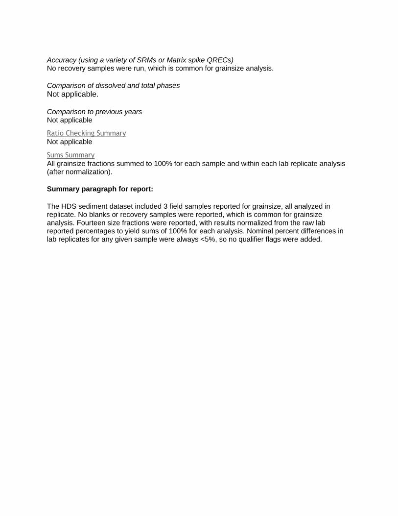
Accuracy (using a variety of SRMs or Matrix spike QRECs) No recovery samples were run, which is common for grainsize analysis. Comparison of dissolved and total phases Not applicable. Comparison to previous years Not applicable
Ratio Checking Summary Not applicable
Sums Summary All grainsize fractions summed to 100% for each sample and within each lab replicate analysis (after normalization). Summary paragraph for report:
The HDS sediment dataset included 3 field samples reported for grainsize, all analyzed in replicate. No blanks or recovery samples were reported, which is common for grainsize analysis. Fourteen size fractions were reported, with results normalized from the raw lab reported percentages to yield sums of 100% for each analysis. Nominal percent differences in lab replicates for any given sample were always <5%, so no qualifier flags were added.

Final Project Report – POC Removal Effectiveness of HDS Units 2019
APPENDIX D: PCBS CONGENERS CONCENTRATION DATA

HDS Site
ID Station Code Sample Date
Collection
Time Matrix PCB Congener(s)
PCB
Concentration
(ng/kg dw) PCB 008 566 PCB 018/30 1,528 PCB 020/28 3,736 PCB 021/33 2,043 PCB 031 2,791 PCB 044/47/65 2,994 PCB 049/69 1,902 PCB 052 3,485 PCB 056 1,681 PCB 060 896 PCB 066 3,472 PCB 070/61/74/76 4,337 PCB 083/99 963 PCB 086/87/97/109/119/125 1,178 PCB 090/101/113 1,552 PCB 093/95/100 1,411 PCB 105 632 PCB 110/115 2,006 PCB 118 1,190 PCB 128/166 323 PCB 129/138/163 2,883 PCB 132 644 PCB 135/151/154 767 PCB 141 353 PCB 147/149 1,564 PCB 153/168 1,785 PCB 156/157 249 PCB 158 190 PCB 170 442 PCB 174 663 PCB 177 340 PCB 180/193 1,583 PCB 183/185 554 PCB 187 1,350 PCB 194 491 PCB 195 172 PCB 201 156 PCB 203 663
1 SUN-MatCDS1 3/8/2018 9:10 AM
Sediment +
Organic
Debris

HDS Site
ID Station Code Sample Date
Collection
Time Matrix PCB Congener(s)
PCB
Concentration
(ng/kg dw) PCB 008 359 PCB 018/30 583 PCB 020/28 863 PCB 021/33 249 PCB 031 842 PCB 044/47/65 1,331 PCB 049/69 1,072 PCB 052 2,662 PCB 056 240 PCB 060 142 PCB 066 635 PCB 070/61/74/76 1,043 PCB 083/99 806 PCB 086/87/97/109/119/125 971 PCB 090/101/113 1,482 PCB 093/95/100 1,353 PCB 105 530 PCB 110/115 1,691 PCB 118 1,151 PCB 128/166 396 PCB 129/138/163 3,094 PCB 132 748 PCB 135/151/154 928 PCB 141 417 PCB 147/149 2,072 PCB 153/168 2,266 PCB 156/157 224 PCB 158 201 PCB 170 770 PCB 174 1,410 PCB 177 641 PCB 180/193 3,683 PCB 183/185 1,281 PCB 187 3,007 PCB 194 1,806 PCB 195 528 PCB 201 415 PCB 203 2,000
2 SUN-MatCDS2 3/8/2018 9:45 AM
Sediment +
Organic
Debris

HDS Site
ID Station Code Sample Date
Collection
Time Matrix PCB Congener(s)
PCB
Concentration
(ng/kg dw) PCB 008 394 PCB 018/30 710 PCB 020/28 821 PCB 021/33 161 PCB 031 752 PCB 044/47/65 1,500 PCB 049/69 900 PCB 052 2,480 PCB 056 548 PCB 060 NDPCB 066 26 PCB 070/61/74/76 2,500 PCB 083/99 3,060 PCB 086/87/97/109/119/125 4,550 PCB 090/101/113 5,890 PCB 093/95/100 4,150 PCB 105 3,830 PCB 110/115 8,890 PCB 118 8,680 PCB 128/166 2,380 PCB 129/138/163 13,000 PCB 132 3,190 PCB 135/151/154 2,610 PCB 141 1,630 PCB 147/149 4,940 PCB 153/168 7,080 PCB 156/157 1,720 PCB 158 NDPCB 170 80 PCB 174 1,330 PCB 177 NDPCB 180/193 NDPCB 183/185 883 PCB 187 1,560 PCB 194 553 PCB 195 211 PCB 201 89 PCB 203 535
3 OAK-5-G 10/16/2017 10:20 AM sediment
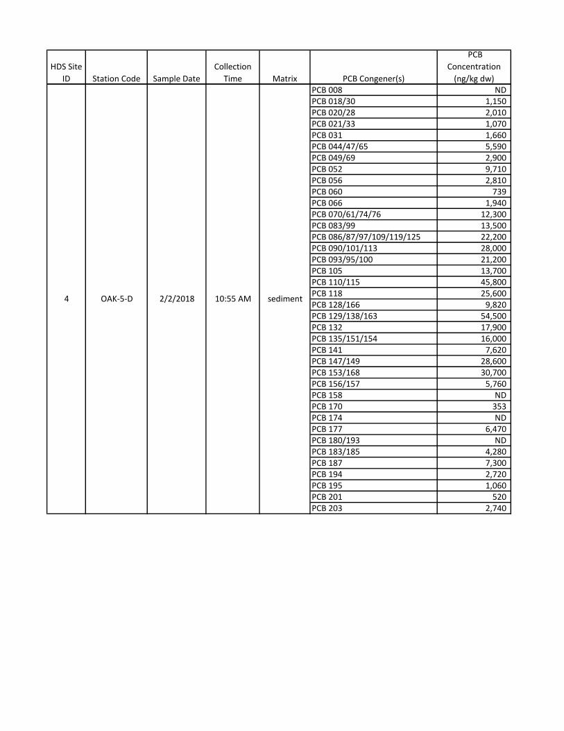
HDS Site
ID Station Code Sample Date
Collection
Time Matrix PCB Congener(s)
PCB
Concentration
(ng/kg dw) PCB 008 NDPCB 018/30 1,150 PCB 020/28 2,010 PCB 021/33 1,070 PCB 031 1,660 PCB 044/47/65 5,590 PCB 049/69 2,900 PCB 052 9,710 PCB 056 2,810 PCB 060 739 PCB 066 1,940 PCB 070/61/74/76 12,300 PCB 083/99 13,500 PCB 086/87/97/109/119/125 22,200 PCB 090/101/113 28,000 PCB 093/95/100 21,200 PCB 105 13,700 PCB 110/115 45,800 PCB 118 25,600 PCB 128/166 9,820 PCB 129/138/163 54,500 PCB 132 17,900 PCB 135/151/154 16,000 PCB 141 7,620 PCB 147/149 28,600 PCB 153/168 30,700 PCB 156/157 5,760 PCB 158 NDPCB 170 353 PCB 174 NDPCB 177 6,470 PCB 180/193 NDPCB 183/185 4,280 PCB 187 7,300 PCB 194 2,720 PCB 195 1,060 PCB 201 520 PCB 203 2,740
4 OAK-5-D 2/2/2018 10:55 AM sediment

HDS Site
ID Station Code Sample Date
Collection
Time Matrix PCB Congener(s)
PCB
Concentration
(ng/kg dw) PCB 008 139 PCB 018/30 193 PCB 020/28 321 PCB 021/33 63 PCB 031 335 PCB 044/47/65 604 PCB 049/69 513 PCB 052 1,182 PCB 056 98 PCB 060 56 PCB 066 287 PCB 070/61/74/76 488 PCB 083/99 431 PCB 086/87/97/109/119/125 490 PCB 090/101/113 682 PCB 093/95/100 651 PCB 105 307 PCB 110/115 911 PCB 118 656 PCB 128/166 NDPCB 129/138/163 1,620 PCB 132 339 PCB 135/151/154 355 PCB 141 168 PCB 147/149 755 PCB 153/168 953 PCB 156/157 140 PCB 158 113 PCB 170 225 PCB 174 264 PCB 177 141 PCB 180/193 672 PCB 183/185 219 PCB 187 516 PCB 194 227 PCB 195 56 PCB 201 52 PCB 203 214
5 PAL-Meadow 10/25/2017 10:50 AM
Sediment +
Organic
Debris

HDS Site
ID Station Code Sample Date
Collection
Time Matrix PCB Congener(s)
PCB
Concentration
(ng/kg dw) PCB 008 4,335 PCB 018/30 5,822 PCB 020/28 11,881 PCB 021/33 3,990 PCB 031 10,761 PCB 044/47/65 12,893 PCB 049/69 9,787 PCB 052 18,317 PCB 056 2,812 PCB 060 1,726 PCB 066 7,505 PCB 070/61/74/76 12,475 PCB 083/99 NDPCB 086/87/97/109/119/125 11,777 PCB 090/101/113 15,545 PCB 093/95/100 12,673 PCB 105 7,492 PCB 110/115 18,274 PCB 118 16,142 PCB 128/166 2,985 PCB 129/138/163 27,208 PCB 132 6,254 PCB 135/151/154 7,046 PCB 141 3,442 PCB 147/149 15,838 PCB 153/168 16,345 PCB 156/157 2,366 PCB 158 1,878 PCB 170 3,446 PCB 174 4,244 PCB 177 2,518 PCB 180/193 7,238 PCB 183/185 3,149 PCB 187 5,990 PCB 194 2,327 PCB 195 779 PCB 201 284 PCB 203 1,777
6 SJC-604 10/5/2017 10:35 AM
Sediment +
Organic
Debris
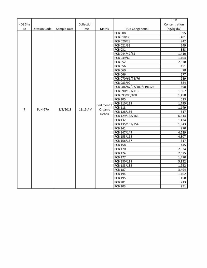
HDS Site
ID Station Code Sample Date
Collection
Time Matrix PCB Congener(s)
PCB
Concentration
(ng/kg dw) PCB 008 395 PCB 018/30 401 PCB 020/28 942 PCB 021/33 149 PCB 031 853 PCB 044/47/65 1,410 PCB 049/69 1,104 PCB 052 2,578 PCB 056 151 PCB 060 78 PCB 066 577 PCB 070/61/74/76 989 PCB 083/99 884 PCB 086/87/97/109/119/125 898 PCB 090/101/113 1,867 PCB 093/95/100 1,458 PCB 105 513 PCB 110/115 1,795 PCB 118 1,149 PCB 128/166 517 PCB 129/138/163 6,614 PCB 132 1,434 PCB 135/151/154 1,843 PCB 141 970 PCB 147/149 4,229 PCB 153/168 4,807 PCB 156/157 317 PCB 158 445 PCB 170 2,024 PCB 174 2,675 PCB 177 1,470 PCB 180/193 5,952 PCB 183/185 1,952 PCB 187 3,494 PCB 194 1,102 PCB 195 458 PCB 201 213 PCB 203 951
7 SUN-27A 3/8/2018 11:15 AM
Sediment +
Organic
Debris

HDS Site
ID Station Code Sample Date
Collection
Time Matrix PCB Congener(s)
PCB
Concentration
(ng/kg dw) PCB 008 24 PCB 018/30 36 PCB 020/28 93 PCB 021/33 42 PCB 031 69 PCB 044/47/65 175 PCB 049/69 92 PCB 052 295 PCB 056 77 PCB 060 42 PCB 066 162 PCB 070/61/74/76 444 PCB 083/99 455 PCB 086/87/97/109/119/125 683 PCB 090/101/113 943 PCB 093/95/100 729 PCB 105 352 PCB 110/115 1,270 PCB 118 879 PCB 128/166 204 PCB 129/138/163 1,330 PCB 132 410 PCB 135/151/154 571 PCB 141 217 PCB 147/149 60 PCB 153/168 843 PCB 156/157 133 PCB 158 125 PCB 170 14 PCB 174 NDPCB 177 328 PCB 180/193 NDPCB 183/185 211 PCB 187 432 PCB 194 186 PCB 195 68 PCB 201 33 PCB 203 179
8 SJC-612-01 9/13/2017 1:53 PM sediment