1

Final Report Mercury in the Environment and Patterns of Mercury Deposition

from the NADP/MDN Mercury Deposition Network

by Tom Butler and Gene Likens (Institute of Ecosystem Studies), Mark Cohen (NOAA Air Resources Lab)

and Françoise Vermeylen (Cornell University)

January 2007 --------------------------------------------------------------

Part 1: A Summary and Review Mercury Emissions, Deposition and Air Chemistry Basic Atmospheric Chemistry Understanding the sources of mercury deposition is fundamental to assessing how to control mercury deposition, in order to protect human health. Uptake of mercury by the general population is largely through fish consumption. The present source of “new mercury” is mainly from atmospheric deposition. However, the sources of deposition in various areas of the country are unclear, and the roles of long-range global transport and deposition versus local and regional deposition are critical questions that are not clearly understood today. Mercury in the atmosphere is largely (~95%) elemental mercury [Hg(0)]. Background concentrations of Hg(0) in the atmosphere are on the order of 1-2 ng/m3 (Slemr and Langer, 1992; Lin and Pehkonen, 1999). It is a gaseous, relatively insoluble form is the form of mercury most subject to long-range transport and least subject to deposition. The overall, global average residence time for Hg(0) is estimated to be as low as 4 to 7 months (Sommar et al. 2001), but is generally considered to be 6 months to 2 years (Schroeder and Munthe 1998).1 Some deposition occurs via stomatal uptake by plants (Mosbaek et al. 1988; Browne and Fang 1978), but the major removal mechanism is by oxidation of Hg(0) to divalent mercury Hg(II), also known as reactive gaseous mercury or RGM, which subsequently deposits. Common oxidants are ozone, and to a lesser extent, the hydroxyl (OH) radical, H2O2 and inorganic halogens. Some recent evidence suggests that the OH radical may not be an important oxidation pathway (Goodsite et al. 2004; Calvert and Lindberg, 2005). Oxidation of Hg(0) to Hg(II) occurs in both the gas phase and the

1 The global average residence time is to be distinguished from “local” residence times. For example, under some localized conditions, the atmospheric lifetime of Hg(0) may be very short, e.g., on the order of minutes to hours, e.g., during mercury depletion events (Lindberg et al., 2002).

2

liquid phase in the atmosphere. Reduction of Hg(II) to Hg(0) also occurs, with the liquid phase reaction with dissolved SO2 believed to be the most important pathway. In marine environments conversion from Hg(0) to RGM can result from interaction with halogen species in the gas and liquid phase (Laurier et al., 2003; Hedgecock and Pirrone, 2001).

RGM species, such as HgCl2 and HgBr2 species, are much “stickier” and more water soluble than Hg(0), and are therefore much more easily dry- and wet-deposited than Hg(0). The typical atmospheric half-life for RGM is on the order of days. RGM in the atmosphere is typically less than 5% of the total mercury, unless near an RGM emission source. Another form of mercury in the atmosphere is particulate mercury [Hg(p)], associated with atmospheric particulate matter. The speciation of Hg(p) is not well known although mercuric oxide (HgO), formed through oxidation of Hg(0) in combustion systems may be an important species (Cohen et al. 2004). The atmospheric residence time of Hg(p) is on the order of one week (EPRI 2004). After wet or dry deposition to land or plant surfaces, oxidized mercury can be reduced back to Hg(0) and re-emitted to the atmosphere, or it can be bound organically and inorganically. In soils and sediments mercury can undergo bacterial conversion to monomethylmercury (CH3HgR where R is a halide such as Cl.), the form of mercury most toxic to organisms. Monomethylmercury bioaccumulates in the aquatic food chain and fish consumption is the major route of uptake by humans. Mercury Emissions A number of different estimates of global mercury emissions are presented in Table 1. Natural and anthropogenic sources are included, and in some cases estimates of mercury re-emission are presented. Direct “current” anthropogenic mercury emissions represent the largest fraction in all but one of the global estimates. In addition, re-emission of mercury may also be largely from previously deposited anthropogenic sources. Seigneur et al. (2003) estimate that 2/3 of re-emissions are originally from anthropogenic sources and re-emissions are responsible for ~½ of the total mercury deposition. Declines in estimates of anthropogenic emissions are at least in part due to efforts to reduce emissions, especially in North America and Europe, as well as declines in mercury emissions with the breakup of the Soviet Union (Slemr et al. 1995). Slemr et al. (1995) notes that the worldwide production of mercury – as a commodity – decreased from 5920 metric tons (mt) in 1989 to 5510 mt in 1990 and to 3650 mt in 1991, due at least in part to efforts to curb the use of mercury. Based on deposition of mercury to glaciers in the western USA, it is estimated that recent peak emissions occurred in the 1980’s (Schuster et al. 2002). Eastern US cores from lakes and bogs show peak deposition in the 1970’s (Norton et al. 1997; Engstrom

3

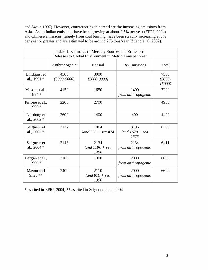
and Swain 1997). However, counteracting this trend are the increasing emissions from Asia. Asian Indian emissions have been growing at about 2.5% per year (EPRI, 2004) and Chinese emissions, largely from coal burning, have been steadily increasing at 5% per year or greater and are estimated to be around 275 tons/year (Zhang et al. 2002).

Table 1. Estimates of Mercury Sources and Emissions Releases to Global Environment in Metric Tons per Year

Anthropogenic Natural Re-Emissions Total

Lindquist et al., 1991 *

4500 (3000-6000)

3000 (2000-9000)

7500 (5000-15000)

Mason et al., 1994 *

4150 1650 1400 from anthropogenic

7200

Pirrone et al., 1996 *

2200 2700 4900

Lamborg et al., 2002 *

2600 1400 400 4400

Seigneur et al., 2003 *

2127 1064 land 590 + sea 474

3195 land 1670 + sea

1575

6386

Seigneur et al., 2004 *

2143 2134 land 1180 + sea

1400

2134 from anthropogenic

6411

Bergan et al., 1999 *

2160 1900 2000 from anthropogenic

6060

Mason and Sheu **

2400 2110 land 810 + sea

1300

2090 from anthropogenic

6600

* as cited in EPRI, 2004; ** as cited in Seigneur et al., 2004

4

Anthropogenic 1998-1999 emissions by continent were estimated by Seigneur et al. (2001) to be:

Continent metric tons/yr Asia 1,117

Africa 246 Europe 327

North America 192 South America and

Central America176

Oceania 48 Total 2,106

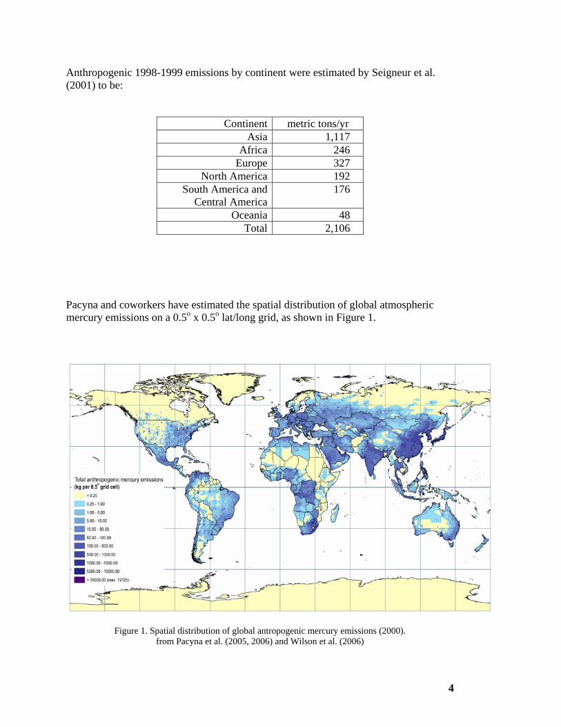
Pacyna and coworkers have estimated the spatial distribution of global atmospheric mercury emissions on a 0.5o x 0.5o lat/long grid, as shown in Figure 1.

Figure 1. Spatial distribution of global antropogenic mercury emissions (2000). from Pacyna et al. (2005, 2006) and Wilson et al. (2006)

5

Per capita emissions of mercury for the U.S., Canada, and China are compared to the global per-capita emissions in Figure 2.

426395

297

360

CHINA_1999 US_1999 CAN_2000 GLOBAL_20000

100

200

300

400

500

(mg

Hg

per p

erso

n-ye

ar)

Anth

ropo

geni

c M

ercu

ry E

mis

sion

sPer Capita Anthropogenic Mercury Emissions

426395

297

360

CHINA_1999 US_1999 CAN_2000 GLOBAL_20000

100

200

300

400

500

(mg

Hg

per p

erso

n-ye

ar)

Anth

ropo

geni

c M

ercu

ry E

mis

sion

sPer Capita Anthropogenic Mercury Emissions

Figure 2. Per-capita emissions of anthropogenic atmospheric mercury emissions. Source of data: 1999 U.S. National Emissions Inventory (U.S. EPA), Environment Canada, Streets et al. (2005), Pacyna et al. (2005, 2006), Wilson et al. (2006).

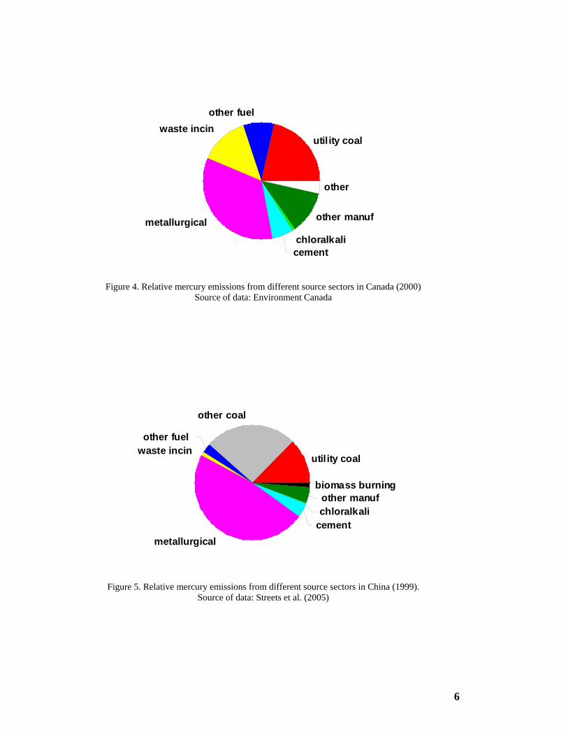
The relative role of different source sectors in contributing mercury emissions varies in different countries. Examples of these different relative contribution patterns are shown below in Figure 3, Figure 4, and Figure 5 for the U.S., Canada, and China, respectively.

utility coal

other coal

other fuel

waste incin

metallurgical cementchloralkali

other manuf

other

Figure 3. Relative mercury emissions from different source sectors in the U.S. (1999) Source of data: U.S. EPA 1999 National Emissions Inventory

6

utility coal

other fuelwaste incin

metallurgical

cementchloralkali

other manuf

other

Figure 4. Relative mercury emissions from different source sectors in Canada (2000) Source of data: Environment Canada

utility coal

other coal

other fuelwaste incin

metallurgicalcementchloralkaliother manuf

biomass burning

Figure 5. Relative mercury emissions from different source sectors in China (1999). Source of data: Streets et al. (2005)

7

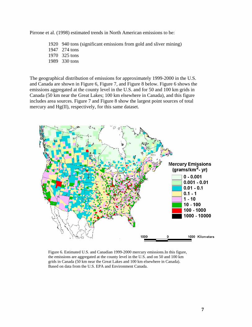
Pirrone et al. (1998) estimated trends in North American emissions to be:

1920 940 tons (significant emissions from gold and sliver mining) 1947 274 tons 1970 325 tons 1989 330 tons

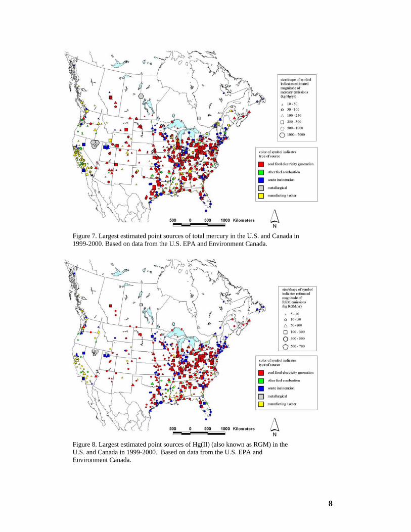
The geographical distribution of emissions for approximately 1999-2000 in the U.S. and Canada are shown in Figure 6, Figure 7, and Figure 8 below. Figure 6 shows the emissions aggregated at the county level in the U.S. and for 50 and 100 km grids in Canada (50 km near the Great Lakes; 100 km elsewhere in Canada), and this figure includes area sources. Figure 7 and Figure 8 show the largest point sources of total mercury and Hg(II), respectively, for this same dataset.

Figure 6. Estimated U.S. and Canadian 1999-2000 mercury emissions.In this figure, the emissions are aggregated at the county level in the U.S. and on 50 and 100 km grids in Canada (50 km near the Great Lakes and 100 km elsewhere in Canada). Based on data from the U.S. EPA and Environment Canada.

8

Figure 7. Largest estimated point sources of total mercury in the U.S. and Canada in 1999-2000. Based on data from the U.S. EPA and Environment Canada.

Figure 8. Largest estimated point sources of Hg(II) (also known as RGM) in the U.S. and Canada in 1999-2000. Based on data from the U.S. EPA and Environment Canada.

9

As the central theme of this analysis is trends, it is important to consider trends in emissions. Unfortunately, there is very little information regarding trends in emissions. In 2005, the EPA stated that it had reliable emissions estimates only for 1990 and 1999 (U.S. EPA 2005a); these estimates are shown in Figure 9.2

1990 19990

50

100

150

200

250

(tons

per

yea

r)E

stim

ated

Mer

cury

Em

issi

ons

Other categories*Gold miningHazardous waste incinerationElectric Arc Furnaces **Mercury Cell Chlor-Alkali PlantsIndustrial, commercial, institutionalboilers and process heatersMunicipal waste combustorsMedical waste incineratorsUtility coal boilers

Figure 9. Anthropogenic mercury emissions data for 1990 and 1999 from the U.S. EPA (2005a). * Data for lime manufacturing are not available for 1990. ** Data for electric arc furnaces are not available for 1999. The 2002 estimate (10.5 tons) is shown here.

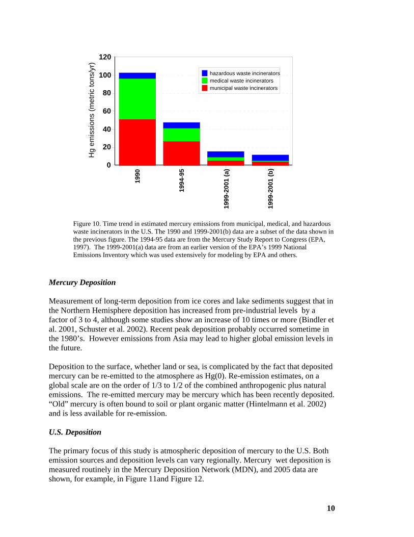
The most significant changes in U.S. emissions since 1990 appear to be for waste incineration. Data for the largest incineration sectors – municipal, medical, and hazardous waste – are presented in Figure 10. This figure also includes estimates for 1994-95, presented by the EPA in the Mercury Study Report to Congress (1997).

2 There appear to be no national emissions estimates available for any time before 1990. The 1996 National Emissions Inventory was withdrawn by EPA due to concerns over data quality. The 2002 National Emissions Inventory has recently been finalized. Summary data for this inventory were requested for the purposes of this report, but have not yet been received.

10

1990

1994

-95

1999

-200

1 (a

)

1999

-200

1 (b

)0

20

40

60

80

100

120

Hg

emis

sion

s (m

etric

tons

/yr)

hazardous waste incineratorsmedical waste incineratorsmunicipal waste incinerators

Figure 10. Time trend in estimated mercury emissions from municipal, medical, and hazardous waste incinerators in the U.S. The 1990 and 1999-2001(b) data are a subset of the data shown in the previous figure. The 1994-95 data are from the Mercury Study Report to Congress (EPA, 1997). The 1999-2001(a) data are from an earlier version of the EPA’s 1999 National Emissions Inventory which was used extensively for modeling by EPA and others.

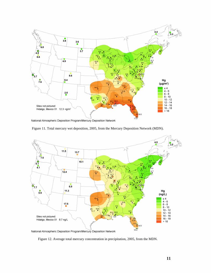
Mercury Deposition Measurement of long-term deposition from ice cores and lake sediments suggest that in the Northern Hemisphere deposition has increased from pre-industrial levels by a factor of 3 to 4, although some studies show an increase of 10 times or more (Bindler et al. 2001, Schuster et al. 2002). Recent peak deposition probably occurred sometime in the 1980’s. However emissions from Asia may lead to higher global emission levels in the future. Deposition to the surface, whether land or sea, is complicated by the fact that deposited mercury can be re-emitted to the atmosphere as Hg(0). Re-emission estimates, on a global scale are on the order of 1/3 to 1/2 of the combined anthropogenic plus natural emissions. The re-emitted mercury may be mercury which has been recently deposited. “Old” mercury is often bound to soil or plant organic matter (Hintelmann et al. 2002) and is less available for re-emission. U.S. Deposition The primary focus of this study is atmospheric deposition of mercury to the U.S. Both emission sources and deposition levels can vary regionally. Mercury wet deposition is measured routinely in the Mercury Deposition Network (MDN), and 2005 data are shown, for example, in Figure 11and Figure 12.

11

Figure 11. Total mercury wet deposition, 2005, from the Mercury Deposition Network (MDN).

Figure 12. Average total mercury concentration in precipitation, 2005, from the MDN.

12

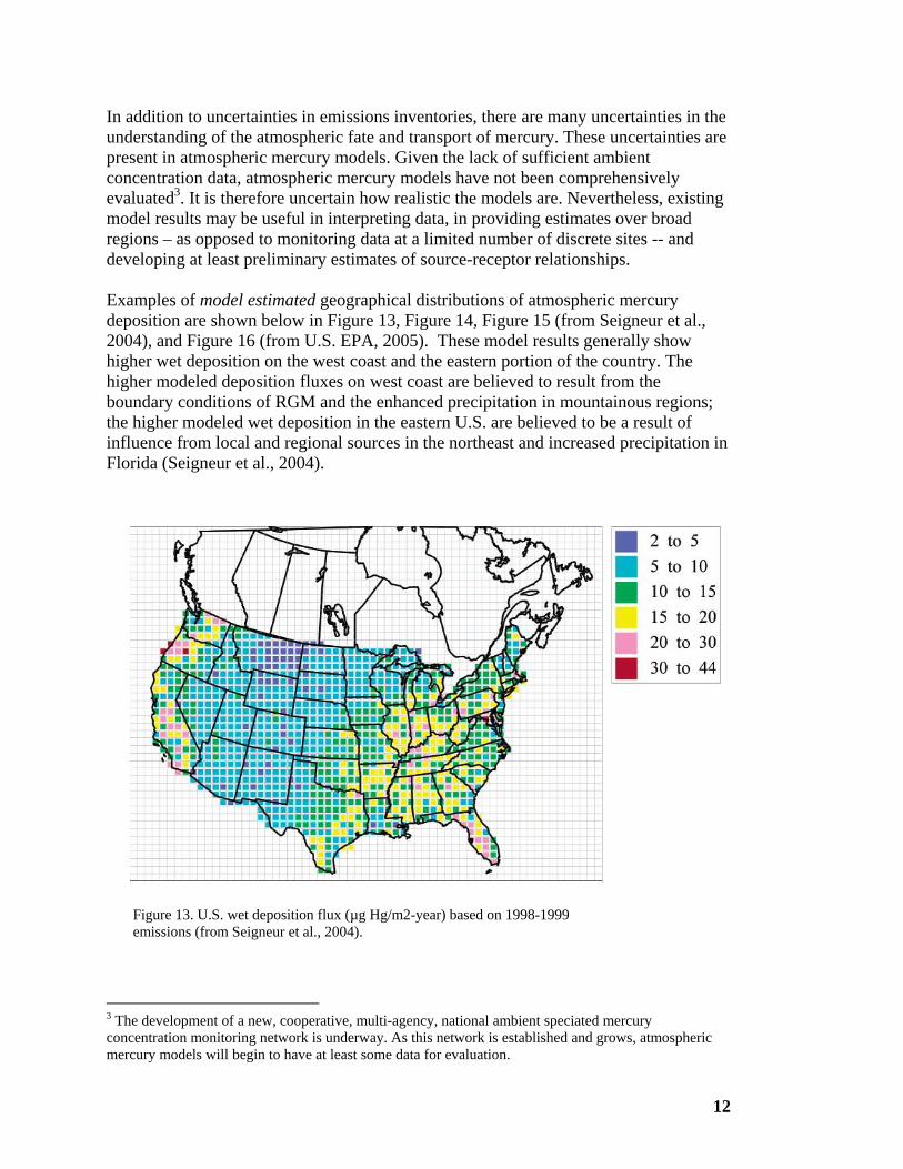
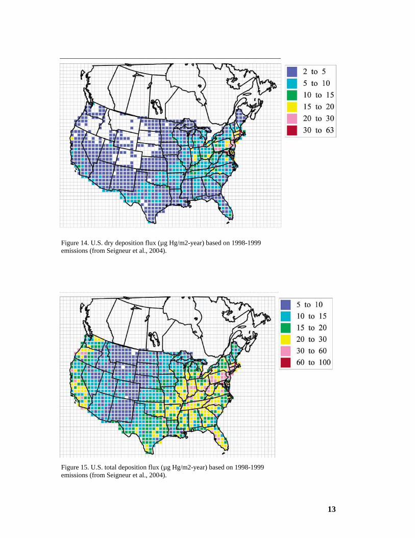
In addition to uncertainties in emissions inventories, there are many uncertainties in the understanding of the atmospheric fate and transport of mercury. These uncertainties are present in atmospheric mercury models. Given the lack of sufficient ambient concentration data, atmospheric mercury models have not been comprehensively evaluated3. It is therefore uncertain how realistic the models are. Nevertheless, existing model results may be useful in interpreting data, in providing estimates over broad regions – as opposed to monitoring data at a limited number of discrete sites -- and developing at least preliminary estimates of source-receptor relationships. Examples of model estimated geographical distributions of atmospheric mercury deposition are shown below in Figure 13, Figure 14, Figure 15 (from Seigneur et al., 2004), and Figure 16 (from U.S. EPA, 2005). These model results generally show higher wet deposition on the west coast and the eastern portion of the country. The higher modeled deposition fluxes on west coast are believed to result from the boundary conditions of RGM and the enhanced precipitation in mountainous regions; the higher modeled wet deposition in the eastern U.S. are believed to be a result of influence from local and regional sources in the northeast and increased precipitation in Florida (Seigneur et al., 2004).

Figure 13. U.S. wet deposition flux (µg Hg/m2-year) based on 1998-1999 emissions (from Seigneur et al., 2004).

3 The development of a new, cooperative, multi-agency, national ambient speciated mercury concentration monitoring network is underway. As this network is established and grows, atmospheric mercury models will begin to have at least some data for evaluation.

13

Figure 14. U.S. dry deposition flux (µg Hg/m2-year) based on 1998-1999 emissions (from Seigneur et al., 2004).

Figure 15. U.S. total deposition flux (µg Hg/m2-year) based on 1998-1999 emissions (from Seigneur et al., 2004).

14

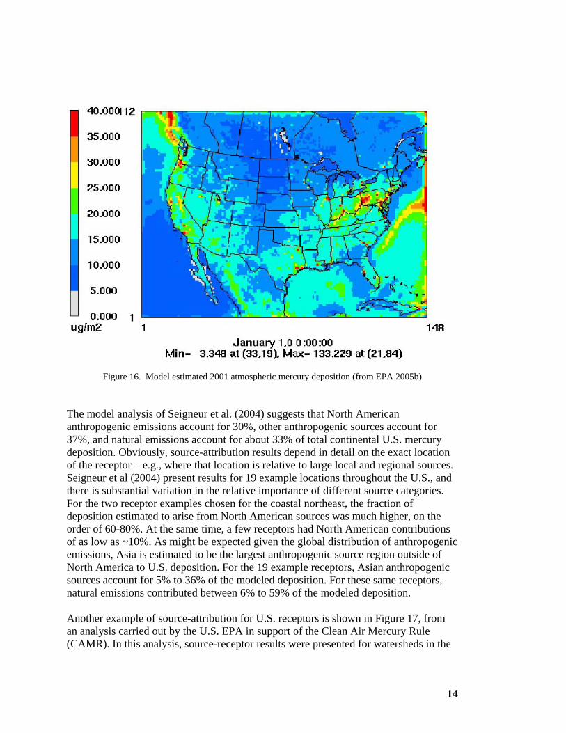
Figure 16. Model estimated 2001 atmospheric mercury deposition (from EPA 2005b) The model analysis of Seigneur et al. (2004) suggests that North American anthropogenic emissions account for 30%, other anthropogenic sources account for 37%, and natural emissions account for about 33% of total continental U.S. mercury deposition. Obviously, source-attribution results depend in detail on the exact location of the receptor – e.g., where that location is relative to large local and regional sources. Seigneur et al (2004) present results for 19 example locations throughout the U.S., and there is substantial variation in the relative importance of different source categories. For the two receptor examples chosen for the coastal northeast, the fraction of deposition estimated to arise from North American sources was much higher, on the order of 60-80%. At the same time, a few receptors had North American contributions of as low as ~10%. As might be expected given the global distribution of anthropogenic emissions, Asia is estimated to be the largest anthropogenic source region outside of North America to U.S. deposition. For the 19 example receptors, Asian anthropogenic sources account for 5% to 36% of the modeled deposition. For these same receptors, natural emissions contributed between 6% to 59% of the modeled deposition. Another example of source-attribution for U.S. receptors is shown in Figure 17, from an analysis carried out by the U.S. EPA in support of the Clean Air Mercury Rule (CAMR). In this analysis, source-receptor results were presented for watersheds in the

15

U.S. -- as defined by Level 8 Hydrologic Unit Code (HUC)4. The extent to which the deposition to each watershed was attributable to electricity generation (“utility”) sources in the U.S. was estimated and the distribution frequency is shown. As an illustration, the “red” line in the figure corresponds to estimated emissions in 2001, and shows, for example, that for 90% of the watersheds, the U.S. utility-attributable deposition accounts for 22% or less of the total model-estimated deposition. Results for potential future emissions scenarios for 2020 are also shown, including estimates accounting for the effects of the Clean Air Interstate Rule, and two different options for the Clean Air Mercury Rule (U.S. EPA 2005b).

Figure 17. Cumulative distribution of percent deposition attributable to U.S. utilities at HUC-8 watershed level in different modeled scenarios (from EPA 2005b).

4 As described in EPA 2005c: “For this analysis, deposition at 36 km grid cells was aggregated to the eight-digit watershed using the ArcMap spatial join function (ESRI, 2004). The HUC, Hydrologic Unit Code, developed by the USGS, spatially delineates watersheds throughout the United States. Hydrologic units are available at four levels of aggregation, ranging from a two-digit regional level (21 units nationwide) to the eight-digit HUC (2,150 distinct units). The eight-digit HUC-level designation is useful for this analysis because it provides a nationally consistent approach for grouping waterbodies on a sufficiently local scale (the average HUC area is 1,631 sq mi). The average deposition for the grid cells that intersect the HUC-8 polygon is then used as the deposition value for the HUC-8 unit. Averaging over grid cells may result in a smoothing out of areas of high and low deposition, because the CMAQ grid cells are smaller than many HUCs.”

16

Guentzel et al. (2001) hypothesize that high-altitude long range-transport of RGM and particulate Hg are a significant source of mercury deposition in Florida. This area consistently has high levels of both concentration and deposition of mercury. It is hypothesized that summertime, tall convective thunderstorms scavenge these species from the upper and middle troposphere, and southeast trade winds regularly resupply RGM to the atmosphere over southern Florida. These summertime storms provide 70% to 90% of the annual mercury deposition in this region. There is also evidence that local/regional emissions in some areas can contribute significantly to mercury deposition. A significant fraction of the RGM that is directly emitted is expected to deposit locally because of its high deposition velocity (similar to that of HNO3) and high solubility (Landis et al. 2002). A large percentage of particulate mercury is also expected to deposit regionally because of its relatively short residence time (a few days) compared to Hg(0). The Florida study above (Guentzel et al. 2001) attributes a large contribution from long-range transport, but also estimates that 30% to 40% of the mercury deposition in Florida is from local anthropogenic sources. Stevens et al. (2000) found that readily deposited RGM represented 75% to 95% of the total mercury emitted from two incinerators in Florida.. Landis et al (2002) investigated the role of the Chicago/Gary urban area on mercury deposition to Lake Michigan and estimated that this area was responsible for elevated levels of both wet and dry deposition to southern Lake Michigan. Wet deposition in the urban area of 26.9 µg/ m2 was almost twice as great as background levels of deposition (14.9 µg/m2) found in northern Michigan. Volume-weighted concentrations of mercury in precipitation were 21.5 ng/l for the Chicago/Gary area as compared with 10.8 ng/l at the northern Michigan location. Particulate and vapor phase mercury concentrations in the atmosphere were also significantly higher near the Chicago/Gary area than at rural sites surrounding Lake Michigan, and air-mass transport studies showed significantly higher Hg(p) concentrations at semi-rural sites along Lake Michigan when trajectories were from the Chicago/Gary area. The lowest concentrations were found when airflows were from the north, where there were few mercury emissions. The highest concentrations of gaseous mercury were also associated with air masses from the Chicago/Gary area. An important conclusion of this study is the need for atmospheric monitoring in and near urban/industrial locations to evaluate the relative importance of local and regional sources to atmospheric Hg deposition. There are few such sites in the existing MDN network. In a complimentary paper Landis and Keeler (2002) estimate that about 20% of the mercury deposition to Lake Michigan is from the Chicago/Gary area. Mason et al. (2000) compared mercury wet deposition at several sites in Maryland and found that rural sites in both eastern and western Maryland had similar fluxes. However an urban site in Baltimore had wet fluxes that were 2 to 3 times higher than the rural sites. In addition, Hg(p) concentrations were 2-3 times higher in Baltimore compared with a rural site on the shore of Chesapeake Bay (Chesapeake Biological Lab). The RGM concentrations were also 2 times higher at the urban site.

17

A study in Steubenville Ohio (Keeler et al., 2006) presents data that suggest local/regional fossil fuel combustion may account for about 70% of the mercury wet deposition. A study in Seattle (Prestbo et al., 2006) found that measured wet deposition declined significantly when local source emissions were decreased. Deposition Trends Several studies have attempted to assess trends (or lack of trends) in mercury concentrations and deposition. Bindler el al. (2001) analyzed sediment cores from 9 Swedish lakes and found temporal and spatial trends. Mercury concentrations in the cores increased 10 fold from 15 to 17 cm to 3 to 1.5 cm, then decreased 15% to 30% toward the sediment surface. Cores taken in 1979 did not show a decline in mercury near the sediment surface. In addition a sharp gradient in Hg concentrations occurs when comparing a site in SW Sweden to sites located in central and northern Sweden. Norton et al. (1997) found cores from ombrotrophic bogs and a lake sediment core in Maine (Acadia National Park) collected in 1983 show a peak in deposition around 1970, followed by significant declines thereafter. Cores taken during approximately the same time from 8 lakes in the Adirondack Mountains of New York also show an increasing trend, and then a decreasing deposition trend in the top 2 cm of the cores (Lorey and Driscoll, 1999). A study in the Midwestern U.S. (Engstrom and Swain 1997) analyzed sediment core data from 4 urban and 8 rural lakes in Minnesota. For the rural lakes, the core data indicated peak mercury deposition in the 1960’s and 1970’s, followed by declines for the rural, eastern Minnesota lakes but not for the western lakes, which are not heavily influenced by local/regional sources. The four urban lakes near Minneapolis show sediment core increases in Hg up to the 1960’s and 1970’s, followed by a sharp decline during the 1980’s. In this same study, sediment cores from 3 lakes in Glacier Bay National Park showed no recent declines in Hg concentration. These cores represent global background mercury deposition. The recent declines in urban and eastern Minnesota sediment cores suggest that the declines are due to local source reductions. The authors estimate that 40% of the total deposition impacting eastern Minnesota are from local anthropogenic sources from the midwestern and eastern U.S. For the period 1990 to 1995 Glass and Sorensen (1999) examined 6 wet deposition sites in the upper Midwest extending from North Dakota to the Upper Peninsula of Michigan. This study showed increasing trends in total mercury deposition of 8% per year on average, and a strong correlation between total mercury and methyl mercury (1.5% of total mercury). When the data are broken up into both warm seasons and cold seasons, both periods show increasing trends from 1990 to 1995. There are also studies that show no recent changes in mercury deposition (usually wet deposition). Keeler et al (2005) examined a site at Underhill, Vermont and found no clear annual trend in wet mercury deposition for the 11-year period from 1993 to 2003

18

(the longest event-based mercury wet deposition record at the time). They also cite a 10-year record (Keeler and Dvonch 2004) for 3 sites in Michigan that show a decreasing wet mercury deposition gradient from south to north, but no clear temporal trend in annual deposition for each site for the period 1994 – 2003. Van Ardsdale et al. (2005) looked for spatial and temporal patterns in mercury deposition and concentrations for northeastern North America for the period 1996 to 2002. Data from the Underhill VT site and data from 13 NADP/MDN (Mercury Deposition Network) sites were used. It is estimated that stationary source emissions in 2002 for NY, NJ and New England were reduced 75% from 1998 emissions (Round and Irvine, 2004). However, these regional reductions were not reflected in the mercury concentration or deposition data. The authors note that Keeler and Yoo (2003) show higher mercury deposition and ambient levels of gaseous and particulate mercury in urban locations compared to rural and remote locations in New England. In addition coastal sites appear to receive more mercury deposition than inland sites (Van Ardsdale et al., unpublished; Ryan et al., 2003). Jaffe et al. (2005) attempted to develop a relation between RGM and particulate Hg emissions (Total Potential Exposure Index or TPEI) and mean concentrations of mercury in precipitation at 28 MDN sites. However, no significant relations were found. The authors hypothesize that possible reasons for this lack of a relation may include differential rainfall rates between sites, different fractions of wet/dry scavenging at different sites, or a relatively large and variable global background contribution.

19

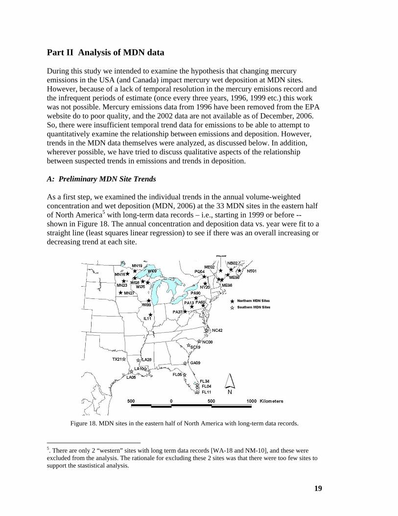
Part II Analysis of MDN data During this study we intended to examine the hypothesis that changing mercury emissions in the USA (and Canada) impact mercury wet deposition at MDN sites. However, because of a lack of temporal resolution in the mercury emisions record and the infrequent periods of estimate (once every three years, 1996, 1999 etc.) this work was not possible. Mercury emissions data from 1996 have been removed from the EPA website do to poor quality, and the 2002 data are not available as of December, 2006. So, there were insufficient temporal trend data for emissions to be able to attempt to quantitatively examine the relationship between emissions and deposition. However, trends in the MDN data themselves were analyzed, as discussed below. In addition, wherever possible, we have tried to discuss qualitative aspects of the relationship between suspected trends in emissions and trends in deposition. A: Preliminary MDN Site Trends As a first step, we examined the individual trends in the annual volume-weighted concentration and wet deposition (MDN, 2006) at the 33 MDN sites in the eastern half of North America5 with long-term data records – i.e., starting in 1999 or before -- shown in Figure 18. The annual concentration and deposition data vs. year were fit to a straight line (least squares linear regression) to see if there was an overall increasing or decreasing trend at each site.

Figure 18. MDN sites in the eastern half of North America with long-term data records.

5. There are only 2 “western” sites with long term data records [WA-18 and NM-10], and these were excluded from the analysis. The rationale for excluding these 2 sites was that there were too few sites to support the stastistical analysis.

20

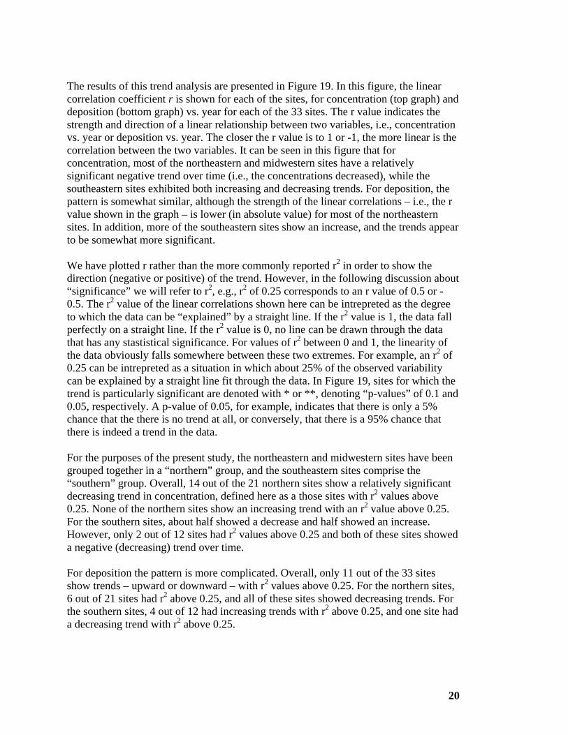
The results of this trend analysis are presented in Figure 19. In this figure, the linear correlation coefficient r is shown for each of the sites, for concentration (top graph) and deposition (bottom graph) vs. year for each of the 33 sites. The r value indicates the strength and direction of a linear relationship between two variables, i.e., concentration vs. year or deposition vs. year. The closer the r value is to 1 or -1, the more linear is the correlation between the two variables. It can be seen in this figure that for concentration, most of the northeastern and midwestern sites have a relatively significant negative trend over time (i.e., the concentrations decreased), while the southeastern sites exhibited both increasing and decreasing trends. For deposition, the pattern is somewhat similar, although the strength of the linear correlations – i.e., the r value shown in the graph – is lower (in absolute value) for most of the northeastern sites. In addition, more of the southeastern sites show an increase, and the trends appear to be somewhat more significant. We have plotted r rather than the more commonly reported r2 in order to show the direction (negative or positive) of the trend. However, in the following discussion about “significance” we will refer to r2, e.g., r2 of 0.25 corresponds to an r value of 0.5 or -0.5. The r2 value of the linear correlations shown here can be intrepreted as the degree to which the data can be “explained” by a straight line. If the r2 value is 1, the data fall perfectly on a straight line. If the r2 value is 0, no line can be drawn through the data that has any stastistical significance. For values of r2 between 0 and 1, the linearity of the data obviously falls somewhere between these two extremes. For example, an r2 of 0.25 can be intrepreted as a situation in which about 25% of the observed variability can be explained by a straight line fit through the data. In Figure 19, sites for which the trend is particularly significant are denoted with * or **, denoting “p-values” of 0.1 and 0.05, respectively. A p-value of 0.05, for example, indicates that there is only a 5% chance that the there is no trend at all, or conversely, that there is a 95% chance that there is indeed a trend in the data. For the purposes of the present study, the northeastern and midwestern sites have been grouped together in a “northern” group, and the southeastern sites comprise the “southern” group. Overall, 14 out of the 21 northern sites show a relatively significant decreasing trend in concentration, defined here as a those sites with r2 values above 0.25. None of the northern sites show an increasing trend with an r2 value above 0.25. For the southern sites, about half showed a decrease and half showed an increase. However, only 2 out of 12 sites had r2 values above 0.25 and both of these sites showed a negative (decreasing) trend over time. For deposition the pattern is more complicated. Overall, only 11 out of the 33 sites show trends – upward or downward – with r2 values above 0.25. For the northern sites, 6 out of 21 sites had r2 above 0.25, and all of these sites showed decreasing trends. For the southern sites, 4 out of 12 had increasing trends with r2 above 0.25, and one site had a decreasing trend with r2 above 0.25.

21

r value for MDN Concentration Trends 1998-2005(-r is declining trend, +r is increasing trend)

* significant slope at p=0.10; **significant slope at p=0.05

-1-0.8-0.6-0.4-0.2

00.20.40.60.8

1

ME02

ME09

ME96

ME98

NB

02

NS01

NY20

PA13

PA37**

PA90*

PA60*

PQ04**

IL11

MN

16*

MN

18*

MN

23**

MN

27

WI08

WI09*

WI36**

WI99

NC

08*

NC

42

FL04

FL05

FL11

FL34

GA

09*

LA05

LA10

LA28

SC19

TX21r v

alue

NE MW SE

r value for MDN Deposition Trends 1998-2005(- r is declining trend, +r is increasing trend)

* significant slope at p=0.10; ** significant slope at p=0.05

-1-0.8-0.6-0.4-0.2

00.20.40.60.8

1

ME02

ME09

ME96

ME98

NB

02

NS01

NY20

PA13

PA37

PA90

PA60

PQ04

IL11

MN

16**

MN

18**

MN

23

MN

27

WI08*

WI09

WI36

WI99*

NC

08*

NC

42

FL04

FL05**

FL11

FL34

GA

09

LA05

LA10

LA28

SC19

TX21r v

alue

NE SEMW

Figure 19. Linear correlation coefficient (r) values for linear regressions of annual mercury precipitation concentration (top graph) and wet deposition (bottom graph) vs. year for individual MDN sites. Sites with trends downward over time have negative values of r, while sites with an increasing trend have positive r values. The r values do not indicate the magnitude of the increasing or decreasing trend for a given site but only indicate the relative confidence that positive or negative linear trend exists. Data are from 1998-2005, unless the site did not operate for this entire period. The sites are divided in Northeast, Midwest, and Southeast regions. Note that for the purposes of the random coefficient analysis presented below, the NE and MW sites were classified as “northern” and the SE sites were classified as “southern”.

22

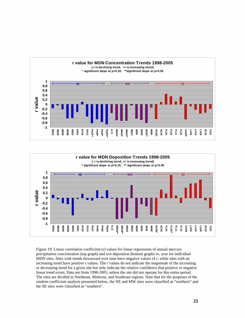
B: MDN trends for the period 1998-2005 using random coefficient statistical models In the analysis above, it was found that there appeared to be geographical differences in deposition trends. However, the stastistical significance of the trend at many of the individual sites was relatively low. An alternative statistical approach is to consider groups of sites using random coefficient models. In essence, this technique assesses the overall trend in the collection of trends in a given group of MDN sites6. In this analysis we considered the same two regions (northeastern= N and southeastern=S) and MDN sites in eastern North America that were considered above. These regions were considered fixed effects in the random coefficient models. The random coefficient models were fit using the Mixed Procedure in SAS (Littell et al. 1996). Further discussions of the random coefficient model are available in Singer (1998), Snijders and Bosker (1999) and Raudenbush and Byrk (2002). For our analysis we used all sites in the eastern US (and southern Canada) with annual data extending back to 1998 for 24 of 32 sites, extending back to 1999 for 6 sites, and extending back to 2000 for 2 sites (See Table 2). The annual data record extends to 2005, except in 4 cases where the record extends to 2004 due to data quality issues or site shutdown. Twenty sites are located in the northeastern group, extending as far south as Virginia, and west to Wisconsin and Illinois. The southeastern quadrant includes sites in North Carolina, Georgia, North Carolina, South Carolina, Louisiana and eastern Texas. The sites are shown in Figure 18, above. The data were analyzed as concentration (ng/liter) vs year and deposition (µg/m2-yr) vs year. The concentration data are volume-weighted means for each year. Concentration and deposition data were also presented in normalized units of “percent of the long-term mean for each site”. When the data are analyzed in this way the slope (x 100) represents the change in concentration or deposition in units of percent change per year. Following similar procedures we also analyzed the data for only the warm months of each year (May through September) when concentrations and deposition are higher compared to the colder months. The list of the data used for the models are presented in Appendix I and Appendix II.

6. Random coefficient models are a statistical approach that assumes that one or more parameters are a random sample from a population of coefficients (slopes and intercepts). In this case each site is a parameter and the regression model for each site represents a random deviation from the model for the population of all sites in the region of interest. Site is considered a random effect because we are not specifically interested in the sites per se, but we consider that these sites are a random sample of all the possible sites where mercury deposition falls in a particular region.

23

Table 2. MDN Sites used for Random Coefficient Models (Start year is 1998 and end year is 2005, unless otherwise noted)

Northern Sites

(n=20) Start Yr End Yr

Southern Sites

(n=12) Start Yr End Yr IL11 1999 FL04

ME02 FL05 ME09 1999 FL11 ME96 FL34 ME98 GA09 MN16 LA05 1999 2004 MN18 LA10 1999 2004 MN23 LA28 1999 2004 MN27 NC08 NB02 NC42 NS01 SC19 NY20 2000 2004 TX21 PA13 PA37 2000 PA90 PQ04 1999 WI08 WI09 WI36 WI99

Results The random coefficient model analysis shows that the northern (N) and southern (S) regions are statistically different from each other. The degree of statistical certainty that the regions are different is expressed as a P-value for a particular comparison, representing the probability that the null hypothesis – i.e., that the overall trends for the two regions are the same -- is true. In the case of annual concentrations, the P-value for the difference between the two regions was 0.003. This means that the probability that the overall regression slope for the two regions are the same is only 0.3%, i.e., it is highly likely that the overall trends for the two regions are different. For annual deposition, the P-value for the overall trend difference between the two regions is 0.005, i.e., there is only a 0.5% chance that the overall trends in deposition in the two regions are the same. Considering warm season (May-Sept) data only, the P-value for concentration is 0.002, and the P-value for deposition is 0.027. In sum, based on this random coefficient statistical analysis, it appears that the two regions are stastically different for both annual and wam-season trends, for both volume-weighted mercury concentrration and mercury deposition. A summary of the results for the overall trends in concentration and deposition using linear models for each region is presented in Table 3. For the northern sites the analysis shows that for the region as a whole there is a decline in concentration of

24

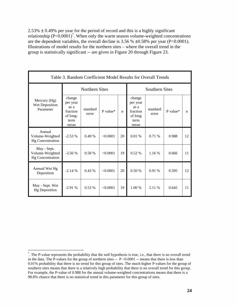
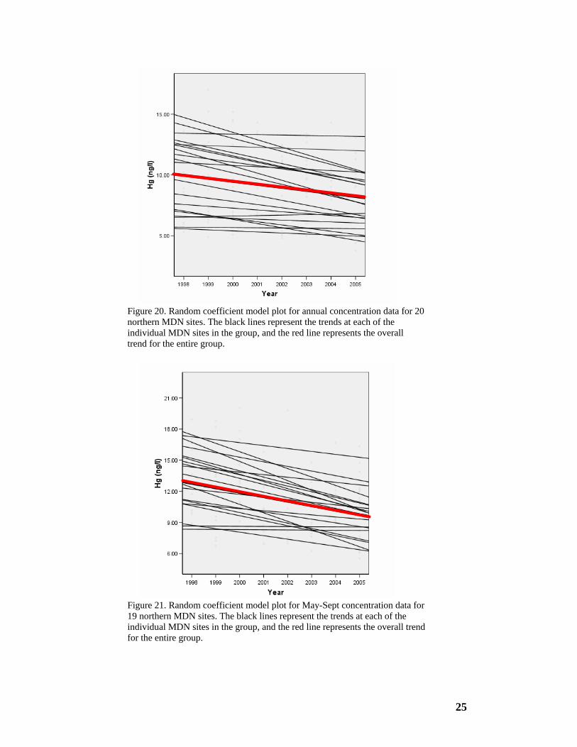
2.53% ± 0.49% per year for the period of record and this is a highly significant relationship (P<0.0001)7. When only the warm season volume-weighted concentrations are the dependent variables, the overall decline is 3.56 % ±0.58% per year (P<0.0001). Illustrations of model results for the northern sites – where the overall trend in the group is statistically significant -- are given in Figure 20 through Figure 23.

Table 3. Random Coefficient Model Results for Overall Trends

Northern Sites Southern Sites

Mercury (Hg) Wet Deposition

Parameter

change per year

as a fraction of long-

term mean

standard error P value* n

change per year

as a fraction of long

term mean

standard error P value* n

Annual Volume-Weighted Hg Concentration

-2.53 % 0.49 % <0.0001 20 0.01 % 0.71 % 0.988 12

May - Sept. Volume-Weighted Hg Concentration

-3.56 % 0.58 % <0.0001 19 0.52 % 1.16 % 0.666 11

Annual Wet Hg Deposition -2.14 % 0.43 % <0.0001 20 0.50 % 0.91 % 0.595 12

May - Sept. Wet Hg Deposition -2.91 % 0.53 % <0.0001 19 1.00 % 2.11 % 0.645 11

7. The P-value represents the probability that the null hypothesis is true, i.e., that there is no overall trend in the data. The P-values for the group of northern sites -- P <0.0001 -- means that there is less than 0.01% probability that there is no trend for this group of sites. The much higher P-values for the group of southern sites means that there is a relatively high probability that there is no overall trend for this group. For example, the P-value of 0.988 for the annual volume-weighted concentrations means that there is a 98.8% chance that there is no statistical trend in this parameter for this group of sites.

25

Figure 20. Random coefficient model plot for annual concentration data for 20 northern MDN sites. The black lines represent the trends at each of the individual MDN sites in the group, and the red line represents the overall trend for the entire group.

Figure 21. Random coefficient model plot for May-Sept concentration data for 19 northern MDN sites. The black lines represent the trends at each of the individual MDN sites in the group, and the red line represents the overall trend for the entire group.

26

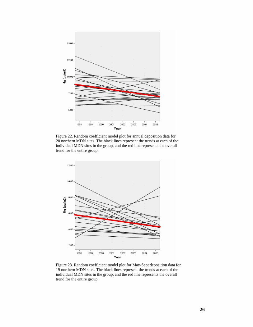
Figure 22. Random coefficient model plot for annual deposition data for 20 northern MDN sites. The black lines represent the trends at each of the individual MDN sites in the group, and the red line represents the overall trend for the entire group.

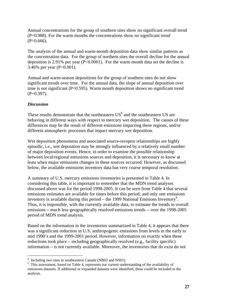
Figure 23. Random coefficient model plot for May-Sept deposition data for 19 northern MDN sites. The black lines represent the trends at each of the individual MDN sites in the group, and the red line represents the overall trend for the entire group.

27

Annual concentrations for the group of southern sites show no significant overall trend (P=0.988). For the warm months the concentrations show no significant trend (P=0.666). The analysis of the annual and warm-month deposition data show similar patterns as the concentration data. For the group of northern sites the overall decline for the annual deposition is 2.91% per year (P<0.0001). For the warm month data set the decline is 3.46% per year (P<0.001). Annual and warm-season depositions for the group of southern sites do not show significant trends over time. For the annual data, the slope of annual deposition over time is not significant (P=0.595). Warm month deposition shows no significant trend (P=0.397). Discussion These results demonstrate that the northeastern US8 and the southeastern US are behaving in different ways with respect to mercury wet deposition. The causes of these differences may be the result of different emissions impacting these regions, and/or different atmospheric processes that impact mercury wet deposition. Wet deposition phenomena and associated source-receptor relationships are highly episodic, i.e., wet deposition may be strongly influenced by a relatively small number of major deposition events. Hence, in order to examine the possible relationship between local/regional emissions sources and deposition, it is necessary to know at least when major emissions changes in these sources occurred. However, as discussed below, the available emissions inventory data has very coarse temporal resolution. A summary of U.S. mercury emissions inventories is presented in Table 4. In considering this table, it is important to remember that the MDN trend analyses discussed above was for the period 1998-2005. It can be seen from Table 4 that several emissions estimates are available for times before this period, and only one emissions inventory is available during this period – the 1999 National Emisions Inventory9. Thus, it is impossible, with the currently available data, to estimate the trends in overall emissions – much less geographically resolved emissions trends -- over the 1998-2005 period of MDN trend analysis. Based on the information in the inventories summarized in Table 4, it appears that there was a significant reduction in U.S. anthropogenic emissions from levels in the early to mid 1990’s and the 1999-2001 period. However, information on exactly when these reductions took place – including geographically resolved (e.g., facility specific) information – is not currently available. Moreover, the inventories that do exist do not

8. Including two sites in southeastern Canada (NB02 and NS01). 9. This assessment, based on Table 4, represents our current understanding of the availability of emissions datasets. If additional or expanded datasets were identified, these could be included in the analysis.

28

provide information on significant changes – e.g., facility maintenance shut-downs – that may occur during the inventoried year. It is therefore very difficult to attempt to relate observed trends at any given MDN site or group of sites to trends in emissions.

Table 4. Summary of U.S. anthropogenic mercury emissions inventories

Inventory

Avail-able for this

study

Geo-graphical resolution

Nominal Time

period for inventory

Total U.S. direct anthro-

pogenic emissions (tons/yr)

Notes and/or References

1990 Cumulative Outdoor Exposure Study

no point and area sources 1990 266 Rosenbaum et al., 1999ab.

1990 National Toxics Inventory (NTI)

yes national totals only 1990 220

EPA (2005a, 2006). These data are shown in Figure 9, above, and are based on the 1990 National Toxics Inventory. We have not been able to find any detailed documentation for this inventory.

Mercury Study Report to Congress (MSRTC, Vol. 2)

yes point and area sources 1994-95* 158

The geographically resolved version of this inventory was used as input to the RELMAP atmospheric fate and transport model (MSTRC, Vol. 3), EPA, 1997. It does not include gold mining, estimated in later inventories to be on the order of 13 tons/year

1996 National Toxics Inventory (NTI)

no

point sources and county-level area sources

1996 195

This inventory has been withdrawn by the EPA due to data quality concerns. The 195 ton total value was obtained from EPA (2006).

hybrid “1996” inventory yes

point sources and county-level area sources

1996 162

used in NOAA atmospheric mercury simulations with the HYSPLIT-Hg model (Cohen et al, 2004). It contains elements of the MSRTC inventory (for municipal and medical waste incinerators and commerical/industrial boilers), 1999 estimates for coal-fired power plants, and the 1996 NTI for other point and area sources.

1999 National Emissions Inventory (NEI)

yes

point sources and county-level area sources

1999 113 some of the incinerator emission reductions may not have occured till 2000-2001

2002 National Emissions Inventory (NEI)

no

point sources and county-level area sources

2002 ? We have been unable to obtain summary or detailed information from this inventory, as of December 2006.

2005 National Emissions Inventory (NEI)

no

point sources and county-level area

sources (?)

2005 ?

This inventory will be released in the future. The EPA reports that it will represent a reduced level of effort, to allow additional resources to be devoted to developing a re-engineered 2008 inventory. Earlier announced plans called for the inventory to be released in Dec 2006, but it does not appear to be available at this time.

* The MSRTC emissions estimates for Municipal Waste Incinerators and Medical Waste Incinerators is possibly more representative of emissions in the early 1990’s.

29

An illustration of this issue is presented in Figure 24 and Figure 25, below. Figure 24 shows long-term MDN sites – generally with a data record going back to 1996 – in the Upper Midwest along with municipal waste and medical waste RGM emissions estimated for the early to mid 1990’s, based on data assembled by the EPA for the Mercury Study Report to Congress (EPA 1997). Also shown are RGM emissions from coal-fired power plants from the 1999 NEI, believed to be somewhat representative of the emissions from the mid-1990’s. In Figure 25 these same MDN sites are shown, with RGM emissions for 1999-2001 are shown, based on data from the EPA’s 1999 National Emissions Inventory (NEI), and the same coal-fired power plant emissions shown in Figure 3. It can be seen from examination of these figures that it is estimated that there were dramatic changes in emissions for waste incinerators in this region. These emissions changes may have had an impact on the wet deposition observed at the MDN sites in the region. However, it is important to know exactly when in the period between the two inventories each major source changed, as the impacts on any given MDN site – and associated wet deposition episodes – may be strongly affected. In future work it would be desirable to examine the history of individual large mercury emissions sources (power plants, incinerators, industrial facilities). Information on the history of major point source Hg emitters may be available in a variety of sources, including, for example, State agencies, the U.S. EPA, industry associations, and the facilities themselves. As mentioned above, Prestbo at el. (2006) found a dramatic drop in mercury concentrations and deposition at MDN site WA18, located northeast of Seattle, after the closure of medical waste incinerators in the Seattle area by 1998. Annual wet mercury concentration and deposition dropped significantly (p < 0.001) from 18.6 ng/l and 16.6 ug/m2-yr, respectively, to 7.86 ng/l and 6.27 ug/m2-yr after 1998. This analysis is a good example of what can be learned from examining the details of when significant emissions changes occurred. Notwithstanding the above limitations, we will briefly examine regional differences in emissions, based on the available data discussed above, and determine if there is any possible relation to the observed trends in MDN data. In this analysis we will consider two inventories – (a) the hybrid inventory believed to be representative of emissions in the early to mid-1990’s described in Cohen et al. (2004) and (b) the 1999 National Emissions Inventory, believed to be representative of emissions in the 1999-2001 period. To provide a crude estimate of regional differences, we divided the eastern half of the US into North and South (North extending from Virginia to Kansas) and totaled the emissions for each inventory for each of these two regions (see Figure 27 below for the extent of each region). As defined, the northeastern region has an area of 2.7 x 106 km2, and the southeastern region has an area of 2.0 x 106 km2.

30

Figure 24. Long-term MDN sites in the Upper Midwest, early to mid 1990’s RGM emissions from municipal and medical waste incinerators emissions inventory developed for the EPA’s Mercury Study Report to Congress, and 1999 RGM emissions from coal-fired power plants.

Figure 25. Long-term MDN sites in the Upper Midwest, 1999-2001 RGM emissions from waste incinerators based on the EPA’s 1999 National Emissions Inventory (NEI), and 1999 RGM emissions from coal-fired power plants based on the EPA’s 1999 NEI.

31

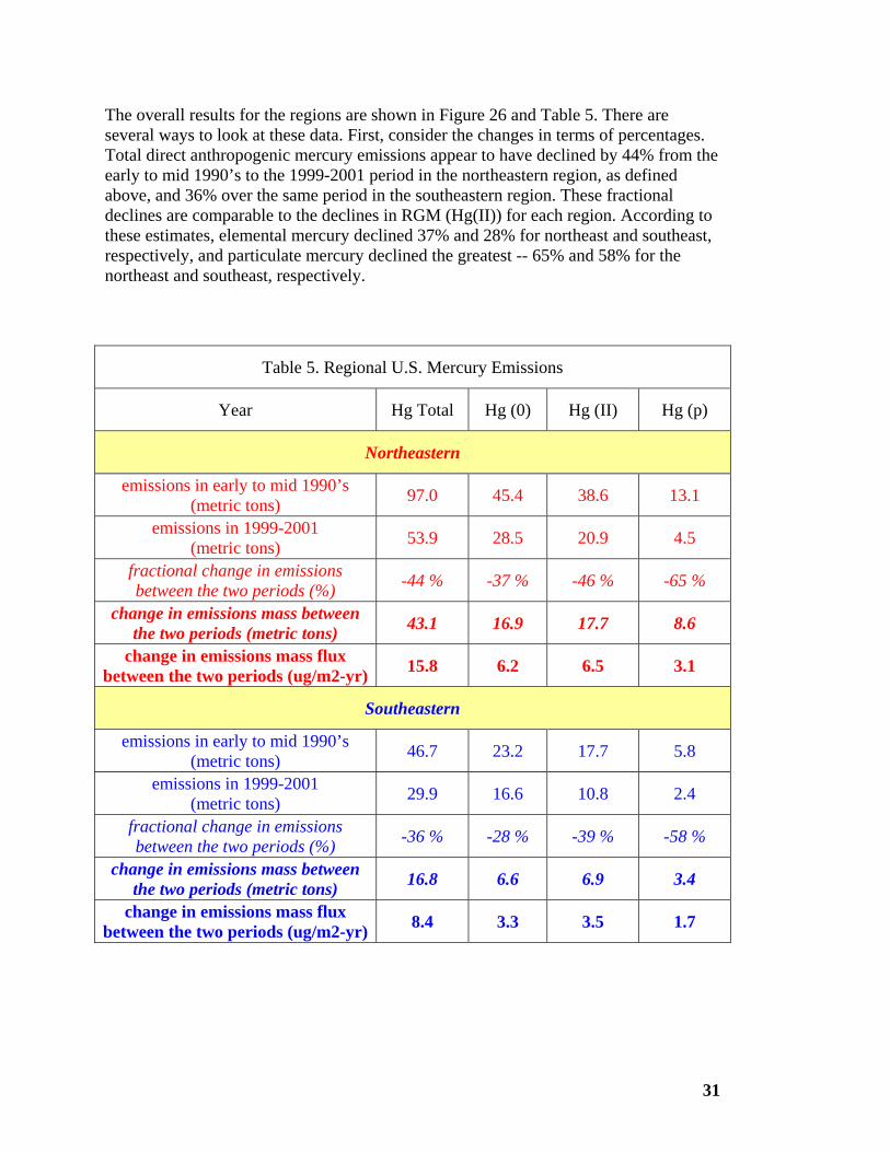
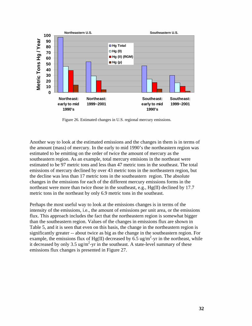
The overall results for the regions are shown in Figure 26 and Table 5. There are several ways to look at these data. First, consider the changes in terms of percentages. Total direct anthropogenic mercury emissions appear to have declined by 44% from the early to mid 1990’s to the 1999-2001 period in the northeastern region, as defined above, and 36% over the same period in the southeastern region. These fractional declines are comparable to the declines in RGM (Hg(II)) for each region. According to these estimates, elemental mercury declined 37% and 28% for northeast and southeast, respectively, and particulate mercury declined the greatest -- 65% and 58% for the northeast and southeast, respectively.

Table 5. Regional U.S. Mercury Emissions

Year Hg Total Hg (0) Hg (II) Hg (p)

Northeastern

emissions in early to mid 1990’s (metric tons) 97.0 45.4 38.6 13.1

emissions in 1999-2001 (metric tons) 53.9 28.5 20.9 4.5

fractional change in emissions between the two periods (%) -44 % -37 % -46 % -65 %

change in emissions mass between the two periods (metric tons) 43.1 16.9 17.7 8.6

change in emissions mass flux between the two periods (ug/m2-yr) 15.8 6.2 6.5 3.1

Southeastern

emissions in early to mid 1990’s (metric tons) 46.7 23.2 17.7 5.8

emissions in 1999-2001 (metric tons) 29.9 16.6 10.8 2.4

fractional change in emissions between the two periods (%) -36 % -28 % -39 % -58 %

change in emissions mass between the two periods (metric tons) 16.8 6.6 6.9 3.4

change in emissions mass flux between the two periods (ug/m2-yr) 8.4 3.3 3.5 1.7

32

0102030405060708090

100

Northeast:early to mid

1990's

Northeast:1999~2001

Southeast:early to mid

1990's

Southeast:1999~2001

Met

ric T

ons

Hg

/ Yea

rHg Total Hg (0)Hg (II) (RGM)Hg (p)

Northeastern U.S. Southeastern U.S.

0102030405060708090

100

Northeast:early to mid

1990's

Northeast:1999~2001

Southeast:early to mid

1990's

Southeast:1999~2001

Met

ric T

ons

Hg

/ Yea

rHg Total Hg (0)Hg (II) (RGM)Hg (p)

Northeastern U.S. Southeastern U.S.

Figure 26. Estimated changes in U.S. regional mercury emissions.

Another way to look at the estimated emissions and the changes in them is in terms of the amount (mass) of mercury. In the early to mid 1990’s the northeastern region was estimated to be emitting on the order of twice the amount of mercury as the southeastern region. As an example, total mercury emisions in the northeast were estimated to be 97 metric tons and less than 47 metric tons in the southeast. The total emissions of mercury declined by over 43 metric tons in the northeastern region, but the decline was less than 17 metric tons in the southeastern region. The absolute changes in the emissions for each of the different mercury emissions forms in the northeast were more than twice those in the southeast, e.g., Hg(II) declined by 17.7 metric tons in the northeast by only 6.9 metric tons in the southeast. Perhaps the most useful way to look at the emissions changes is in terms of the intensity of the emissions, i.e., the amount of emissions per unit area, or the emissions flux. This approach includes the fact that the northeastern region is somewhat bigger than the southeastern region. Values of the changes in emissions flux are shown in Table 5, and it is seen that even on this basis, the change in the northeastern region is significantly greater -- about twice as big as the change in the southeastern region. For example, the emissions flux of Hg(II) decreased by 6.5 ug/m2-yr in the northeast, while it decreased by only 3.5 ug/m2-yr in the southeast. A state-level summary of these emissions flux changes is presented in Figure 27.

33

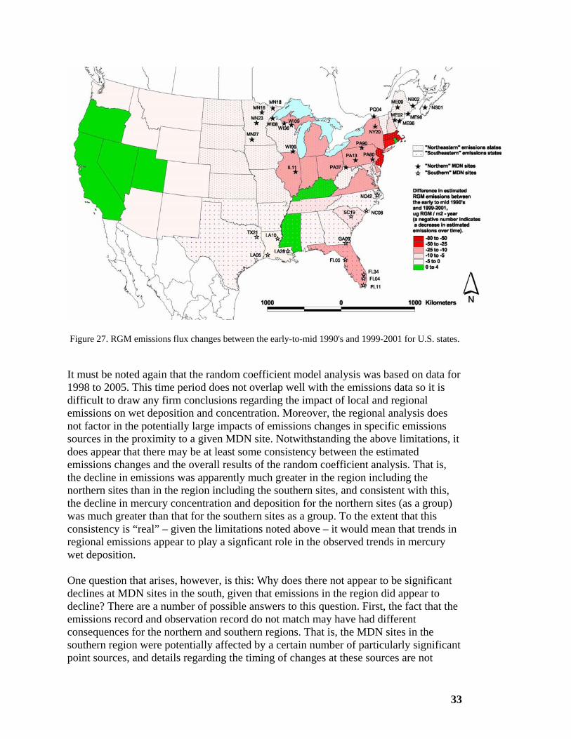
Figure 27. RGM emissions flux changes between the early-to-mid 1990's and 1999-2001 for U.S. states.

It must be noted again that the random coefficient model analysis was based on data for 1998 to 2005. This time period does not overlap well with the emissions data so it is difficult to draw any firm conclusions regarding the impact of local and regional emissions on wet deposition and concentration. Moreover, the regional analysis does not factor in the potentially large impacts of emissions changes in specific emissions sources in the proximity to a given MDN site. Notwithstanding the above limitations, it does appear that there may be at least some consistency between the estimated emissions changes and the overall results of the random coefficient analysis. That is, the decline in emissions was apparently much greater in the region including the northern sites than in the region including the southern sites, and consistent with this, the decline in mercury concentration and deposition for the northern sites (as a group) was much greater than that for the southern sites as a group. To the extent that this consistency is “real” – given the limitations noted above – it would mean that trends in regional emissions appear to play a signficant role in the observed trends in mercury wet deposition. One question that arises, however, is this: Why does there not appear to be significant declines at MDN sites in the south, given that emissions in the region did appear to decline? There are a number of possible answers to this question. First, the fact that the emissions record and observation record do not match may have had different consequences for the northern and southern regions. That is, the MDN sites in the southern region were potentially affected by a certain number of particularly significant point sources, and details regarding the timing of changes at these sources are not

34

known. The same problem exists for the northern MDN sites. The point here is that the overall impact of this limitation may be different in the north than in the south. Another potential answer is that mercury wet deposition at some or all of the southern sites may be governed by different atmospheric processes. Guentzel et al. (2001) propose that high altitude long-range transport of RGM and particulate Hg are a significant source of mercury deposition in Florida. Again this is due to summertime large convective storms that scavenge globally derived RGM and particulate mercury from the middle and upper troposphere. These storms also occur in other southeastern areas where intense summer heating leads to major convective activity, in some cases on a near daily basis (for example states bordering the Gulf of Mexico). However these exceptionally tall storms are not as likely in the cooler northeastern quarter of the country, where convective activity is not as intense. Therefore this upper level source of mercury is perhaps less available to these areas. If global sources play a bigger role in deposition in the southeastern states, then declines in local emissions may be offset by increases in global emission sources. While some global emissions are decreasing, such as in Europe, other global sources of mercury emissions are significantly increasing. India, China and other Southeast Asian countries experiencing rapid growth have increasing mercury emissions, largely from greater coal burning. In fact, even if global sources have approximately the same impact at the northern and southern sites investigated in this study, the results still may be consistent with the general conclusion that local and regional emissions sources exert a strong influence on the observed wet deposition. For both the southern and northern sites, the increase in global emissions would have led to the same overall increase in the contribution of this component of the total deposition. For the southern sites, the decrease in regional emissions was only moderate, and this decrease more or less balanced the increase in global contribution. For the northern sites, the decrease was much larger, and the decrease would have more than compensated for the increase in the global source contribution.

35

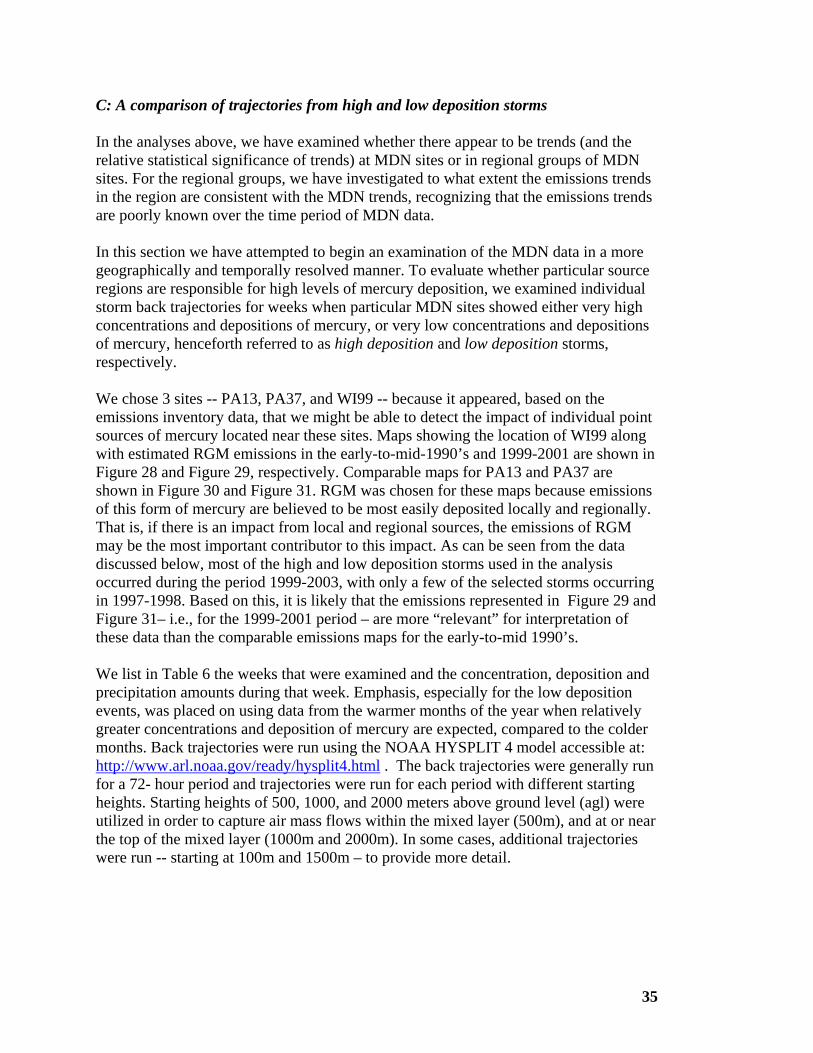
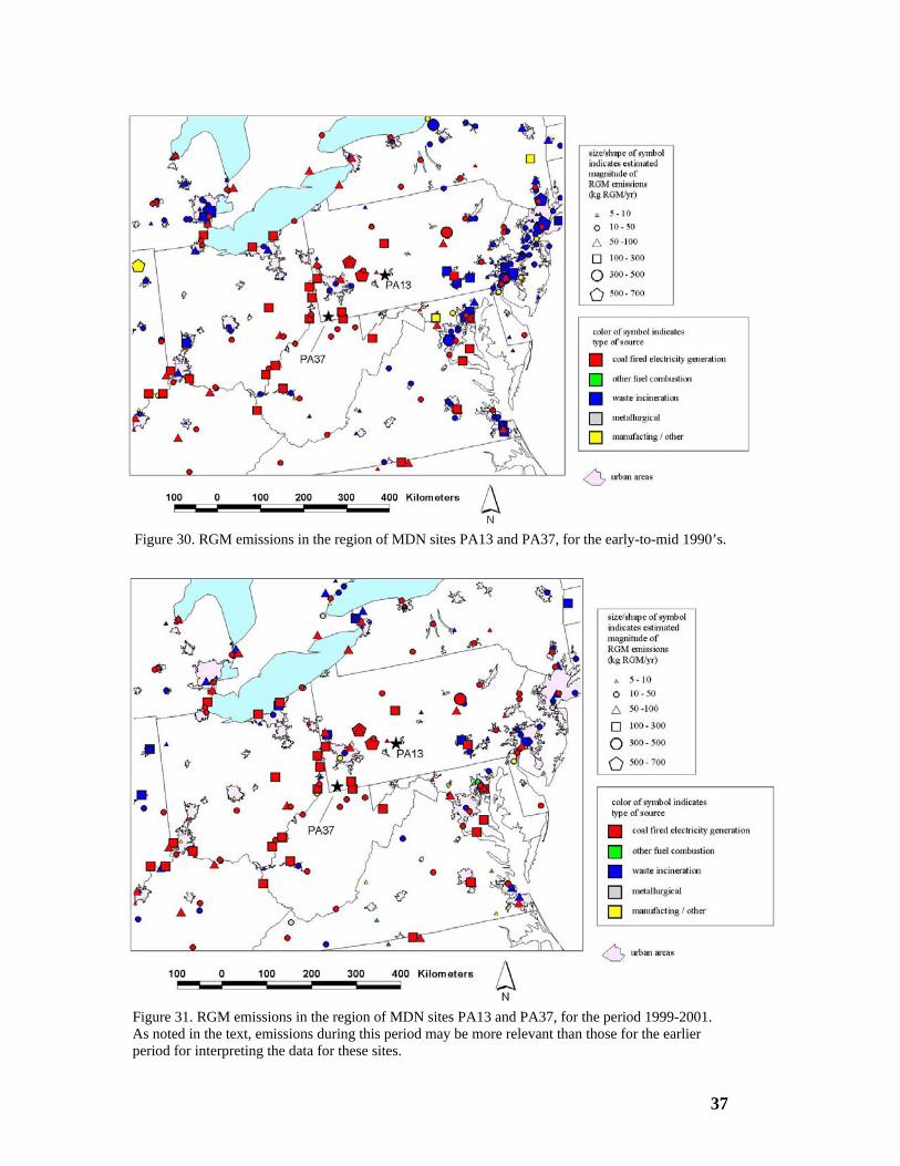
C: A comparison of trajectories from high and low deposition storms In the analyses above, we have examined whether there appear to be trends (and the relative statistical significance of trends) at MDN sites or in regional groups of MDN sites. For the regional groups, we have investigated to what extent the emissions trends in the region are consistent with the MDN trends, recognizing that the emissions trends are poorly known over the time period of MDN data. In this section we have attempted to begin an examination of the MDN data in a more geographically and temporally resolved manner. To evaluate whether particular source regions are responsible for high levels of mercury deposition, we examined individual storm back trajectories for weeks when particular MDN sites showed either very high concentrations and depositions of mercury, or very low concentrations and depositions of mercury, henceforth referred to as high deposition and low deposition storms, respectively. We chose 3 sites -- PA13, PA37, and WI99 -- because it appeared, based on the emissions inventory data, that we might be able to detect the impact of individual point sources of mercury located near these sites. Maps showing the location of WI99 along with estimated RGM emissions in the early-to-mid-1990’s and 1999-2001 are shown in Figure 28 and Figure 29, respectively. Comparable maps for PA13 and PA37 are shown in Figure 30 and Figure 31. RGM was chosen for these maps because emissions of this form of mercury are believed to be most easily deposited locally and regionally. That is, if there is an impact from local and regional sources, the emissions of RGM may be the most important contributor to this impact. As can be seen from the data discussed below, most of the high and low deposition storms used in the analysis occurred during the period 1999-2003, with only a few of the selected storms occurring in 1997-1998. Based on this, it is likely that the emissions represented in Figure 29 and Figure 31– i.e., for the 1999-2001 period – are more “relevant” for interpretation of these data than the comparable emissions maps for the early-to-mid 1990’s. We list in Table 6 the weeks that were examined and the concentration, deposition and precipitation amounts during that week. Emphasis, especially for the low deposition events, was placed on using data from the warmer months of the year when relatively greater concentrations and deposition of mercury are expected, compared to the colder months. Back trajectories were run using the NOAA HYSPLIT 4 model accessible at: http://www.arl.noaa.gov/ready/hysplit4.html . The back trajectories were generally run for a 72- hour period and trajectories were run for each period with different starting heights. Starting heights of 500, 1000, and 2000 meters above ground level (agl) were utilized in order to capture air mass flows within the mixed layer (500m), and at or near the top of the mixed layer (1000m and 2000m). In some cases, additional trajectories were run -- starting at 100m and 1500m – to provide more detail.

36

Figure 28. RGM emissions in the region of MDN site WI99, for the early-to-mid 1990’s.

Figure 29. RGM emissions in the region of MDN site WI99, for the period 1999-2001. As noted in the text, emissions during this period may be more relevant than those for the earlier period for interpreting the data for this site.

37

Figure 30. RGM emissions in the region of MDN sites PA13 and PA37, for the early-to-mid 1990’s.

Figure 31. RGM emissions in the region of MDN sites PA13 and PA37, for the period 1999-2001. As noted in the text, emissions during this period may be more relevant than those for the earlier period for interpreting the data for these sites.

38

Table 6 High and Low Deposition weeks for PA37, PA13 and WI99

Low Deposition Weeks High Deposition Weeks Date On Precip Conc. Deposition Date On Precip Conc DepositionSite (mm) (ng/l) ng/m2 (mm) (ng/l) ng/m2

PA37 10/15/02 39.1 2.0 79.8 5/5/03 99.1 14.1 1398.8 PA37 9/10/02 27.2 4.5 123.3 5/7/02 81.5 12.8 1040.9 PA37 9/14/99 21.3 5.2 111.5 7/1/03 54.5 18.2 992.4 PA37 4/8/03 13.6 5.7 77.0 8/24/99 40.0 20.8 830.5 PA37 9/20/03 11.2 6.5 72.1 4/18/00 11.4 62.6 715.3 PA37 5/28/02 15.6 7.0 108.6 4/28/03 41.9 16.9 710.3 PA37 4/17/01 17.1 7.7 131.5 7/27/99 25.9 22.1 573.3 PA37 8/31/99 20.2 7.9 160.4 7/31/01 15.1 24.1 364.5 PA37 5/21/02 10.2 8.8 89.2 7/6/99 14.9 22.5 336.4 PA37 10/8/02 16.0 8.8 140.4 10/26/99 33.1 9.5 314.2 PA37 9/23/03 10.4 9.7 100.7 4/10/01 34.0 15.5 525.9 PA37 3/27/01 8.6 5.0 43.1 6/13/00 42.4 16.3 689.6 PA37 10/22/02 8.7 5.4 47.2 4/30/02 24.4 18.7 456.9 PA37 4/3/01 23.1 16.8 387.4 PA37 8/21/01 18.3 19.9 364.6

PA13 9/23/97 65.5 2.2 141.5 4/10/01 52.7 60.4 3183.7 PA13 3/16/99 19.7 2.2 44.2 5/15/01 9.5 124.1 1182.1 PA13 3/9/99 13.3 2.4 32.1 6/19/01 53.6 16.8 899.5 PA13 3/31/98 29.8 3.6 108.9 5/13/97 57.2 15.4 879.7 PA13 10/15/02 29.2 4.3 126.1 7/6/99 25.5 21.9 558.2 PA13 9/9/97 38.4 4.5 171.7 4/4/01 25.4 21.0 534.5 PA13 8/31/99 39.3 4.9 191.3 3/12/02 25.1 20.8 522.1 PA13 10/16/01 9.9 4.9 49.0 7/31/01 21.3 20.5 435.8 PA13 10/22/02 19.6 5.3 103.8 7/23/02 16.1 23.2 374.5 PA13 4/28/98 24.6 5.6 137.0 5/11/99 14.0 22.2 310.4 PA13 10/22/03 23.1 5.7 130.7 7/30/02 16.8 20.8 348.8 PA13 9/29/98 17.7 6.6 117.3 7/11/00 13.0 23.9 310.0 PA13 4/13/99 21.8 7.4 161.8 7/27/99 18.7 23.1 431.3 PA13 4/4/00 15.1 7.8 117.2 12/16/97 7.9 48.5 384.8 PA13 7/1/97 15.9 7.0 111.5 11/23/99 56.4 6.6 374.1

WI99 3/17/98 18.0 3.6 64.6 6/24/98 94.2 25.0 2360.3 WI99 9/17/02 36.6 4.8 175.9 4/17/01 26.2 83.0 2171.4 WI99 6/3/03 23.6 6.4 150.1 5/30/00 72.4 21.2 1537.5 WI99 8/5/97 24.1 6.9 165.7 4/16/02 26.2 42.9 1122.2 WI99 4/4/00 27.2 7.0 190.0 7/1/03 48.8 25.1 1226.3 WI99 5/21/02 18.0 7.5 136.0 9/8/98 43.2 21.4 924.5 WI99 8/28/01 23.9 7.7 184.5 4/6/99 33.0 24.3 802.4 WI99 8/7/01 12.7 9.7 122.9 6/17/97 17.8 36.6 649.9 WI99 4/23/02 14.2 9.8 139.8 5/12/98 26.7 23.0 612.5 WI99 8/6/02 10.2 10.1 102.5 8/18/98 9.4 39.3 369.8 WI99 7/13/99 11.4 12.7 145.6 4/18/00 84.1 17.3 1453.2 WI99 9/7/99 8.9 4.8 42.4 10/24/00 33.9 21.5 730.1 WI99 5/2/00 31.8 20.9 662.8 WI99 5/19/98 26.7 20.3 542.4 WI99 7/31/01 31.8 19.7 626.8

39

The MDN data are weekly and this presents a challenge for storm-based analysis. In an attempt to at least partially compensate for this limitation, rain gauge charts were obtained from the NADP Program Office at the Illinois State Water Survey for each week and examined to determine the times for storm events in order to calculate the appropriate back trajectories. The hour to start the back trajectory was chosen from the rain gauge charts and the time selected was either the middle of a precipitation event, or during the period of maximum precipitation rate. Many of the weeks had more than one storm so there was more than one back trajectory calculated in such weeks, with the assumption that high or low concentrations occurred in all storms for a particular week. In most cases back trajectories within the same week were from similar directions. In addition, when a storm was of long duration (for example > 8 hours) then more than one back trajectory was calculated to see whether significant wind shifts occurred during a storm. In general that was not the case. Air mass back trajectories usually did not change substantially during a rain event. Obviously, event-based precipitation samples would be more useful for this type of analysis, but we have attempted this limited analysis with the weekly MDN data. For PA37, PA13 and WI99 combined, a total of 45 and 41 weeks were examined for high and low deposition storms, respectively. During these weeks a total of 89 high deposition and 49 low deposition storms were assessed. We summarize in Table 6 the mean precipitation and volume-weighted mean concentrations and deposition for both high deposition and low deposition weeks at each of the three sites examined. The concentrations were 3 to 6 times higher and the wet deposition was 6 to 8 times higher for the high vs low storms, respectively. Precipitation was 1 to 2 times higher for the low deposition storms when compared to the high deposition storms.

Table 7 Volume-weighted mean concentration and deposition values for high and low deposition storms

Site Storm Type

Concentration (ng/l)

Deposition (ng/m2-wk)

Precipitation (mm/wk)

PA37 Low 5.9 98.8 16.9

PA37 High 17.3 646.7 37.3

PA13 Low 4.5 116.3 25.5

PA13 High 26.0 715.3 27.5

WI99 Low 7.1 135.0 19.1

WI99 High 26.1 1052.8 40.4

40

It is important at the outset to note several limitations of this more detailed analysis based on back-trajectories, including, but not limited to the following:

• The absence of high deposition storms from a given direction may simply mean that due to typical weather patterns, large storms generally didn’t approach the site from that direction.

• Many storms do not appear to have a readily discernable “direction”, as back trajectories starting at different heights diverge markedly as they move backwards from the MDN site.

• We have selected a number of storms as examples, but it is not certain that the selected storms are completely representative of the entire data set of observations.

• While every effort was made to choose representative trajectories for a given storm, it is recognized that different starting times and different starting heights might yield somewhat different trajectories.

• It is difficult to assess the relative importance of the trajectories starting at different heights above the source for a given precipitation event at the MDN site, as this would depend on the detailed structure of the storm. Thus, some of the trajectories examined may be essentially irrelevant for the precipitation occurring at the site (e.g., a trajectory might be above and not interacting with the precipitating cloud layer).

• In a related manner, the effects of vertical mixing along the trajectories are difficult to incorporate or otherwise interpret in the analysis. For example, the ability of mercury emitted by a source to be entrained in an air mass depends on the vertical mixing at the source location and downwind of the source. In some cases, a trajectory may appear to pass over a source, and one might expect the source to contribute mercury to the air mass. However, if the vertical mixing was limited, and the emissions occurred below or above the air mass, they may not have been entrained in the air mass.

• It is difficult to estimate the impact of wet deposition along the trajectory. If the storm produced significant precipitation on its way to the MDN site, some or all of the mercury that might have been entrained from local and regional sources may be depleted. Ideally, one would have an accurate record of the precipitation encountered by the trajectory on its way to the monitoring site. The archived, gridded meteorological data used to estimate the trajectories does have gridded precipitation data and these data can be used to estimate the potential importance of this effect. However, the gridded precipitation data in these datasets can be somewhat inaccurate as it is generally based on forecasts and the resolution (e.g., 40km or 80km) of the grid is somewhat coarse. We found for example that for some of the trajectories, the meteorological data indicated that there was no precipitation at the MDN site when the storm was occurring.

• It is difficult to estimate the impact of dry deposition along the trajectory in terms of depletion of mercury – particularly reactive gaseous mercury, the form of mercury most readily wet deposited – before the air mass arrives at the site. This issue is related to the vertical mixing issues discussed above. If the air

41

mass passed near the ground or was in a mixing layer that contacted the ground, then significant dry deposition would be possible.

• As with all comparable back-trajectory analyses, effects of atmospheric chemistry are not accounted for. If there is any significant oxidation or reduction of mercury forms in the plume, this would certainly affect the deposition.

An approach that at least partially avoids many of the above difficulties uses deterministic forward-dispersion models to simulate the atmospheric fate and transport of emissions from each source. The HYSPLIT-Hg model (Cohen et al., 2004) and the CMAQ-Hg model (Bullock and Brehme, 2002) are examples of this type of model. Nevertheless, in spite of the above issues, we have attempted to determine if an examination of back-trajectories associated with high and low deposition storms at the selected MDN sites will yield any information on the possible impact of local and regional sources. However, given the above issues, this back-trajectory analysis must be regarded as being somewhat preliminary and qualitative. It may be possible to develop a more refined analysis in future work. Results Examination of individual storm tracks for the selected high wet deposition and low wet deposition events did appear to show some interesting patterns. First, we attempted to characterize the storms by their general direction. In some cases, the storms were relatively slow moving, and tended to have trajectories arriving from a number of different directions. For these storms, it was not easy to characterize them by a certain direction. However, we classified them due to their slow moving nature as being relatively “stagnant”. For these storms, most or all of the back-trajectories stayed within 600-1200 km of the MDN site over 72 hours. Several examples of these storms will be presented below. The overall results of this initial atttempt at classifying the different storms in the high and low deposition groups are shown in Figure 32 and Figure 33. There are of course a number of other factors that influence mercury wet deposition and these will also be discussed below. For sites PA13 and PA37, it is likely that storms from the west-southwest and south-southwest have the potential to be high deposition events as there are a large number of significant mercury sources at these directions from the sites (see Figure 31 above). In addition, for PA37, the west-northwest direction appears to contain a number of particularly large mercury sources. Unlike PA13 and PA37, areas west-southwest of WI99 do not appear to have a significant number of mercury sources (see Figure 29 above). Moreover, the region west-northwest does not appear to contain significant sources, at least in the 1999-2001 inventory. Thus the general patterns shown in Figure 32 for the three sites are consistent with the geographical distribution of regional mercury sources. WI99 does show a similar pattern with PA13 and PA37, in that slow moving air masses often with multi-directional trajectories occur in over 40% of the

42

high deposition storms. For PA13 and PA37 50% and 34% have these types of back trajectories.

High Concentration, High Deposiition Storms(PA13 n=28,16wks; PA37 n=34,14wks; WI99 n=27,15wks)

0

10

20

30

40

50

60

S-SW

S-SE

W-SW

W-NW

Coastal

Stagnan

t

% o

f Sto

rms

PA13PA37WI99

Figure 32. Percent of high concentration and high wet mercury deposition storms with back trajectories from particular source areas, for sites PA13, PA37 and WI99.

Low Concentration, Low Deposition Storms(PA13 n=17,16wk; PA37 n=18;13wks; WI99 n=14,11wks)

0

10

20

30

40

50

60

S-SW

S-SE

W-SW

W-NW

Coastal

Stagnan

t

% o

f Sto

rms

PA13PA37WI99

Figure 33. Percent of low concentration and low wet mercury deposition storms with back trajectories from particular source areas, for sites PA13, PA37 and WI99.

43

High deposition, high concentration storms For high concentration, high deposition storms, the geographical pattern shown in Figure 32 appears to be more or less consistent with the distribution of mercury sources in the region around each particular MDN site. Figure 30 and Figure 31 suggest that for PA13, storms from the northwest and southwest might be strongly influenced by local and regional sources. A somewhat comparable pattern would be expected for PA37, although the lack of high deposition storms clearly identifiable as being from the south-southeast and east-southeast is perhaps surprising for this site. However, examination of the above figures suggests that the east-southeast direction might contain relatively high local impacts, and none of the storms examined in this preliminary analysis were classified as coming uniformly from that direction. Additional aspects of potential local and regional source contributions will be discussed below in the context of multi-directional storms. Figure 28 and Figure 29 suggest that for WI99, storms from a number of directions – including southeast, southwest, and northeast -- might contain significant contributions from local and regional mercury sources. The overall pattern shown in Figure 32 for WI99 is somewhat consistent with the geographical distribution of sources around the site but additional complexities – including the impacts of multi-directional storms – will be discussed below. As noted earlier, a relatively large fraction of the storms (~30-50%) at each of the sites were “stagnant”, relatively slow moving, multi-directional air flows. In some cases, we have classified storms in this category if the absolute distance traveled away from the site was relatively low even if the “speed” of the trajectories was not parrticularly slow (i.e., storms that more or less tended to meander around within the region of the MDN site). As noted above, for these storms, most or all of the back-trajectories stayed within 600-1200 km of the MDN site over 72 hours. Since these storms do not have an obvious directional interpretation, they will be discussed in some detail here. First, all things being equal, such storms might be said to have the greatest potential for high concentrations and deposition of mercury. This is because mercury emitted and entrained in a fast moving storm is relatively diluted, but the same amount of mercury emitted and entrained in a slow moving storm would result in a much higher mercury concentration. Thus, it is not surprising that many of the high deposition weeks that we examined appeared to be related to slow moving storms. Such storms would also be expected to be high in other atmospheric pollutants (SO4

=, NO3- and H+) as well as mercury. In future work it would be possible to examine

other precipitation chemistry species in these same high and low mercury deposition weeks.

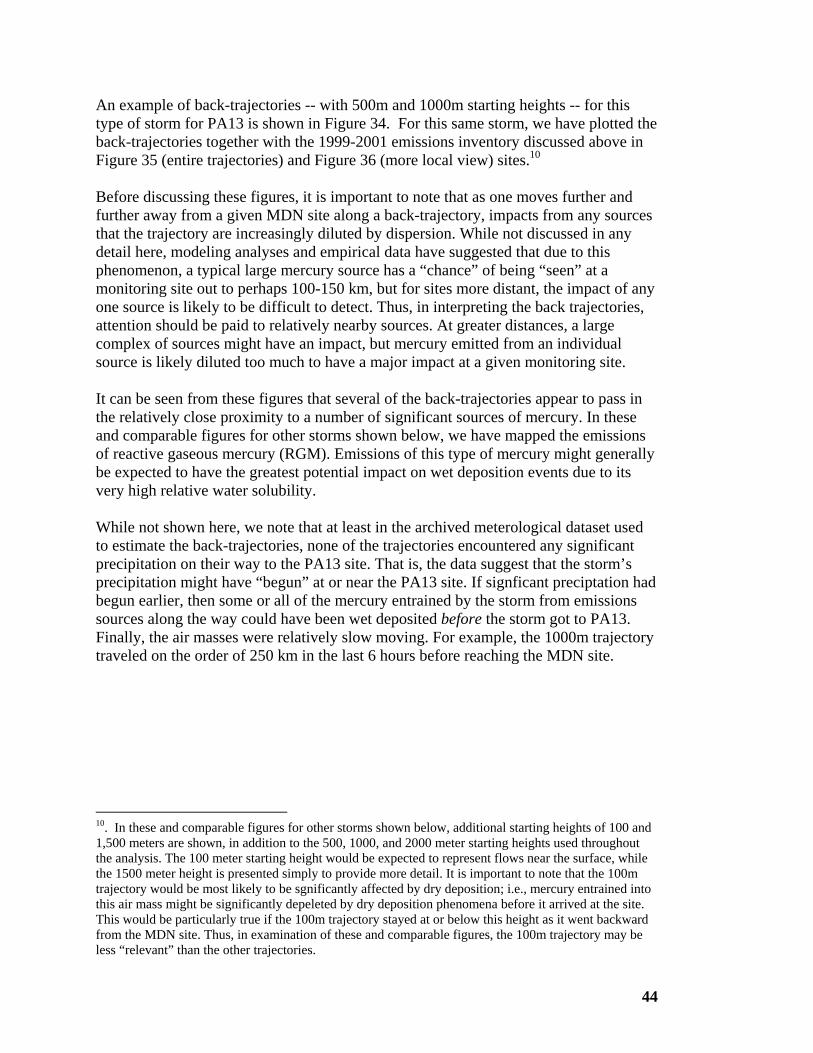
44

An example of back-trajectories -- with 500m and 1000m starting heights -- for this type of storm for PA13 is shown in Figure 34. For this same storm, we have plotted the back-trajectories together with the 1999-2001 emissions inventory discussed above in Figure 35 (entire trajectories) and Figure 36 (more local view) sites.10 Before discussing these figures, it is important to note that as one moves further and further away from a given MDN site along a back-trajectory, impacts from any sources that the trajectory are increasingly diluted by dispersion. While not discussed in any detail here, modeling analyses and empirical data have suggested that due to this phenomenon, a typical large mercury source has a “chance” of being “seen” at a monitoring site out to perhaps 100-150 km, but for sites more distant, the impact of any one source is likely to be difficult to detect. Thus, in interpreting the back trajectories, attention should be paid to relatively nearby sources. At greater distances, a large complex of sources might have an impact, but mercury emitted from an individual source is likely diluted too much to have a major impact at a given monitoring site. It can be seen from these figures that several of the back-trajectories appear to pass in the relatively close proximity to a number of significant sources of mercury. In these and comparable figures for other storms shown below, we have mapped the emissions of reactive gaseous mercury (RGM). Emissions of this type of mercury might generally be expected to have the greatest potential impact on wet deposition events due to its very high relative water solubility. While not shown here, we note that at least in the archived meterological dataset used to estimate the back-trajectories, none of the trajectories encountered any significant precipitation on their way to the PA13 site. That is, the data suggest that the storm’s precipitation might have “begun” at or near the PA13 site. If signficant preciptation had begun earlier, then some or all of the mercury entrained by the storm from emissions sources along the way could have been wet deposited before the storm got to PA13. Finally, the air masses were relatively slow moving. For example, the 1000m trajectory traveled on the order of 250 km in the last 6 hours before reaching the MDN site.

10. In these and comparable figures for other storms shown below, additional starting heights of 100 and 1,500 meters are shown, in addition to the 500, 1000, and 2000 meter starting heights used throughout the analysis. The 100 meter starting height would be expected to represent flows near the surface, while the 1500 meter height is presented simply to provide more detail. It is important to note that the 100m trajectory would be most likely to be sgnificantly affected by dry deposition; i.e., mercury entrained into this air mass might be significantly depeleted by dry deposition phenomena before it arrived at the site. This would be particularly true if the 100m trajectory stayed at or below this height as it went backward from the MDN site. Thus, in examination of these and comparable figures, the 100m trajectory may be less “relevant” than the other trajectories.

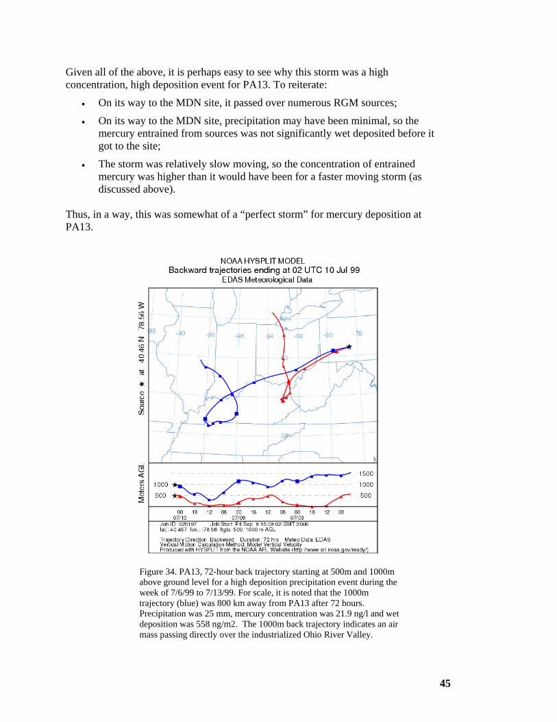
45

Given all of the above, it is perhaps easy to see why this storm was a high concentration, high deposition event for PA13. To reiterate:

• On its way to the MDN site, it passed over numerous RGM sources;

• On its way to the MDN site, precipitation may have been minimal, so the mercury entrained from sources was not significantly wet deposited before it got to the site;

• The storm was relatively slow moving, so the concentration of entrained mercury was higher than it would have been for a faster moving storm (as discussed above).

Thus, in a way, this was somewhat of a “perfect storm” for mercury deposition at PA13.

Figure 34. PA13, 72-hour back trajectory starting at 500m and 1000m above ground level for a high deposition precipitation event during the week of 7/6/99 to 7/13/99. For scale, it is noted that the 1000m trajectory (blue) was 800 km away from PA13 after 72 hours. Precipitation was 25 mm, mercury concentration was 21.9 ng/l and wet deposition was 558 ng/m2. The 1000m back trajectory indicates an air mass passing directly over the industrialized Ohio River Valley.

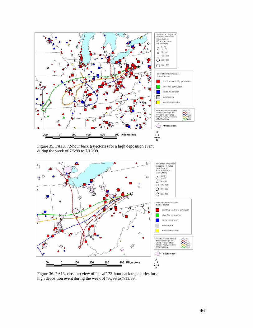
46

Figure 35. PA13, 72-hour back trajectories for a high deposition event during the week of 7/6/99 to 7/13/99.

Figure 36. PA13, close-up view of “local” 72-hour back trajectories for a high deposition event during the week of 7/6/99 to 7/13/99.

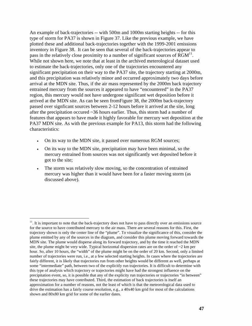
47

An example of back-trajectories -- with 500m and 1000m starting heights -- for this type of storm for PA37 is shown in Figure 37. Like the previous example, we have plotted these and additional back-trajectories together with the 1999-2001 emissions inventory in Figure 38. It can be seen that several of the back-trajectories appear to pass in the relatively close proximity to a number of significant sources of RGM11. While not shown here, we note that at least in the archived meterological dataset used to estimate the back-trajectories, only one of the trajectories encountered any significant precipitation on their way to the PA37 site, the trajectory starting at 2000m, and this precipitation was relatively minor and occurred approximately two days before arrival at the MDN site. Thus, if the air mass represented by the 2000m back trajectory entrained mercury from the sources it appeared to have “encountered” in the PA37 region, this mercury would not have undergone significant wet deposition before it arrived at the MDN site. As can be seen fromFigure 38, the 2000m back-trajectory passed over signficant sources between 2-12 hours before it arrived at the site, long after the precipitation occured ~36 hours earlier. Thus, this storm had a number of features that appears to have made it highly favorable for mercury wet deposition at the PA37 MDN site. As with the previous example for PA13, this storm had the following characteristics:

• On its way to the MDN site, it passed over numerous RGM sources;

• On its way to the MDN site, precipitation may have been minimal, so the mercury entrained from sources was not significantly wet deposited before it got to the site;

• The storm was relatively slow moving, so the concentration of entrained mercury was higher than it would have been for a faster moving storm (as discussed above).

11. It is important to note that the back-trajectory does not have to pass directly over an emissions source for the source to have contributed mercury to the air mass. There are several reasons for this. First, the trajectory shown is only the center line of the “plume”. To visualize the significance of this, consider the plume emitted by any of the sources in the diagram, and consider this plume moving forward towards the MDN site. The plume would disperse along its forward trajectory, and by the time it reached the MDN site, the plume might be very wide. Typical horizontal dispersion rates are on the order of ~2 km per hour. So, after 10 hours, the “width” of the plume might be on the order of 20 km. Second, only a limited number of trajectories were run, i.e., at a few selected starting heights. In cases where the trajectories are fairly different, it is likely that trajectories run from other heights would be different as well, perhaps at some “intermediate” path, between two of the explicitly run trajectories. It is difficult to determine with this type of analysis which trajectory or trajectories might have had the strongest influence on the precipitation event, so, it is possible that any of the explicity run trajectories or trajectories “in between” these trajectories may have contributed. Third, the estimation of back trajectories is itself an approximation for a number of reasons, not the least of which is that the meteorological data used to drive the estimation has a fairly course resolution, e.g., a 40x40 km grid for most of the calculations shown and 80x80 km grid for some of the earlier dates.

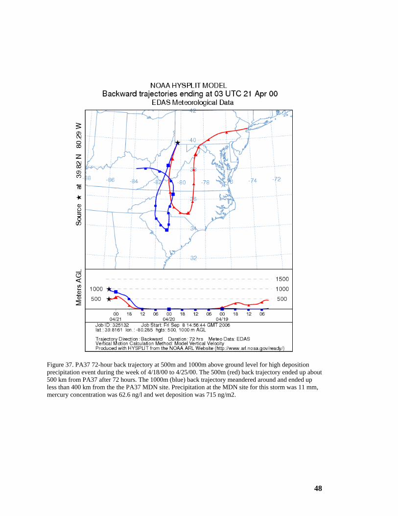
48

Figure 37. PA37 72-hour back trajectory at 500m and 1000m above ground level for high deposition precipitation event during the week of 4/18/00 to 4/25/00. The 500m (red) back trajectory ended up about 500 km from PA37 after 72 hours. The 1000m (blue) back trajectory meandered around and ended up less than 400 km from the the PA37 MDN site. Precipitation at the MDN site for this storm was 11 mm, mercury concentration was 62.6 ng/l and wet deposition was 715 ng/m2.

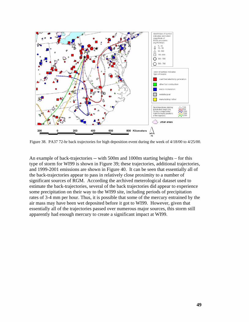
49

Figure 38. PA37 72-hr back trajectories for high deposition event during the week of 4/18/00 to 4/25/00. An example of back-trajectories -- with 500m and 1000m starting heights – for this type of storm for WI99 is shown in Figure 39; these trajectories, additional trajectories, and 1999-2001 emissions are shown in Figure 40. It can be seen that essentially all of the back-trajectories appear to pass in relatively close proximity to a number of significant sources of RGM. According the archived meterological dataset used to estimate the back-trajectories, several of the back trajectories did appear to experience some precipitation on their way to the WI99 site, including periods of precipitation rates of 3-4 mm per hour. Thus, it is possible that some of the mercury entrained by the air mass may have been wet deposited before it got to WI99. However, given that essentially all of the trajectories passed over numerous major sources, this storm still apparently had enough mercury to create a significant impact at WI99.

50

Figure 39. WI99, 72-hour back trajectory for high deposition precipitation event during the week of 4/18/00 to 4/25/00. Precipitation was 84 mm, mercury concentration was 17.3 ng/l and wet deposition was 1453 ng/m2. . The 1000-m back trajectory (blue) shows air mass near ground passing over Chicago/Gary metropolitan area.

51

Figure 40. WI99, 72-hour back trajectories for high deposition event during the week of 4/18/00 to 4/25/00.

In addition to the relatively slow moving, multi-directional storms discussed above, high deposition storms also commonly arrive from the south-southwest direction, especially for WI99, where over 40% of the high deposition storms examined were classified in this category. At WI99, such storm tracks can be influenced by the mercury emission sources in the Chicago/ Gary area, a region which contributes significantly to mercury deposition to Lake Michigan (Landis et al. 2002). In addition, there are other sources in the south-southwest “region” relative to the WI99 site, and these might also contribute.12 One example of such a storm is presented in Figure 41 – for 500m, 1000m, and 1500m back-trajectories -- and in Figure 42 with 1999-2001 emissions. Unlike the previous examples, it can be seen that all of the trajectories traverse a very similar path. Thus, this storm could be classified as coming from a certain “direction”, i.e., in this case, from the south-southwest direction. Over 72 hours, the air mass travelled about 1200 km, a distance comparable to the other relatively slow moving storms. It can be seen that several of the trajectories -- and particularly the 500m and 100m trajecrtories – appear to pass in the relative close proximity to a number of significant RGM sources.

12. We note that the storm “classification” system used here has its limitations. For example, in essentially all of the the “stagnant, multi-directional” storms discussed above, one or more trajectories did have a certain degree of south-southwestern influence. However, since the trajectories were not “consistently” travelling in this direction, the storms were not classified in this category. Nevertheless, the same group of sources -- in the south-southwest direction – may have been contributing significantly in these examples as well.

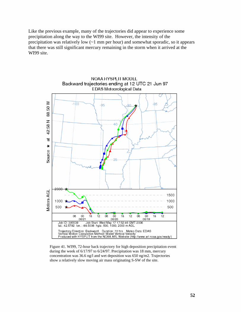
52

Like the previous example, many of the trajectories did appear to experience some precipitation along the way to the WI99 site. However, the intensity of the precipitation was relatively low (~1 mm per hour) and somewhat sporadic, so it appears that there was still significant mercury remaining in the storm when it arrived at the WI99 site.

Figure 41. WI99, 72-hour back trajectory for high deposition precipitation event during the week of 6/17/97 to 6/24/97. Precipitation was 18 mm, mercury concentration was 36.6 ng/l and wet deposition was 650 ng/m2. Trajectories show a relatively slow moving air mass originating S-SW of the site.

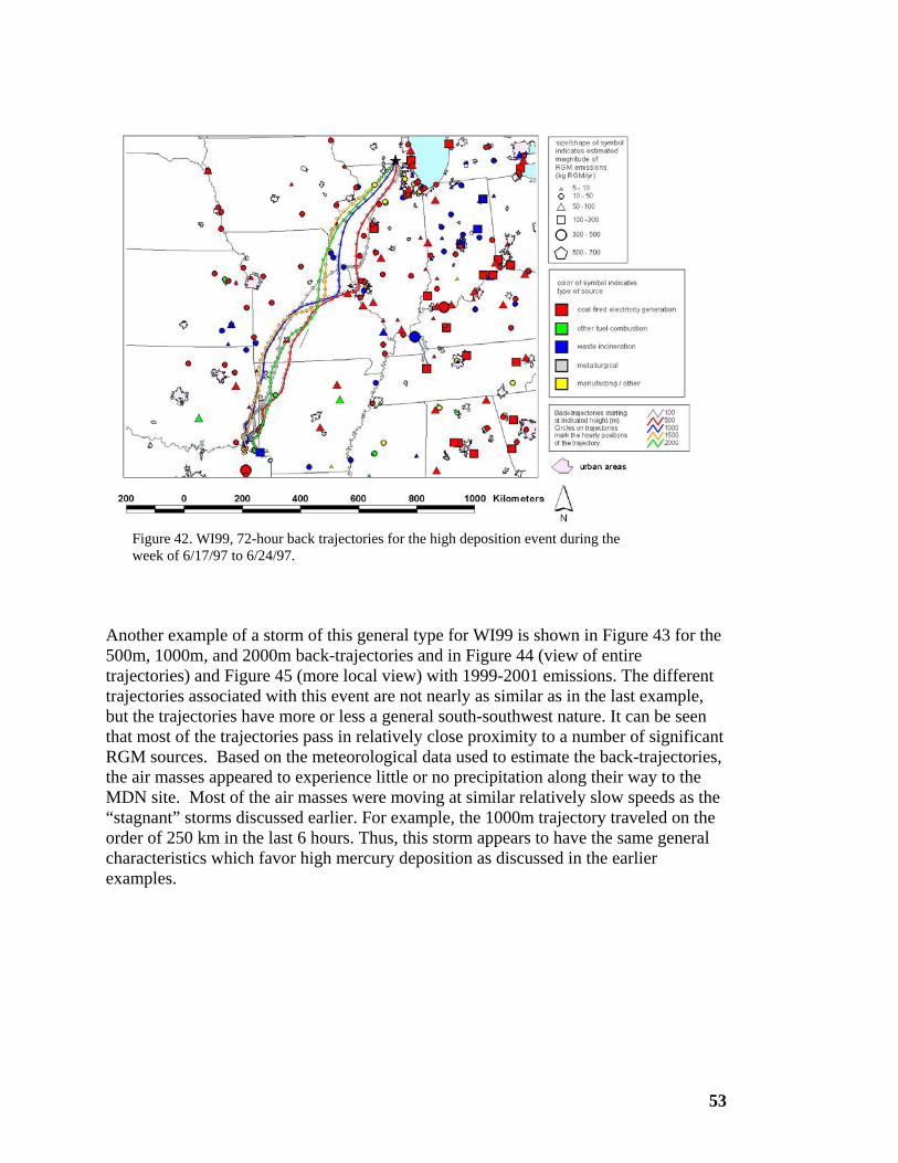
53

Figure 42. WI99, 72-hour back trajectories for the high deposition event during the week of 6/17/97 to 6/24/97.

Another example of a storm of this general type for WI99 is shown in Figure 43 for the 500m, 1000m, and 2000m back-trajectories and in Figure 44 (view of entire trajectories) and Figure 45 (more local view) with 1999-2001 emissions. The different trajectories associated with this event are not nearly as similar as in the last example, but the trajectories have more or less a general south-southwest nature. It can be seen that most of the trajectories pass in relatively close proximity to a number of significant RGM sources. Based on the meteorological data used to estimate the back-trajectories, the air masses appeared to experience little or no precipitation along their way to the MDN site. Most of the air masses were moving at similar relatively slow speeds as the “stagnant” storms discussed earlier. For example, the 1000m trajectory traveled on the order of 250 km in the last 6 hours. Thus, this storm appears to have the same general characteristics which favor high mercury deposition as discussed in the earlier examples.

54

Figure 43. WI99, 72-hour back trajectory for high deposition precipitation event during the week of 5/12/98 to 5/19/98. Total precipitation for the week was 26.7 mm, and the concentration and deposition were 23.0 ng/l and 612.5 ug/m2 for the week. There were two storms during the week, and the back-trajectories in this figure represent the largest storm, with a total of 18.1 mm of precipitation.

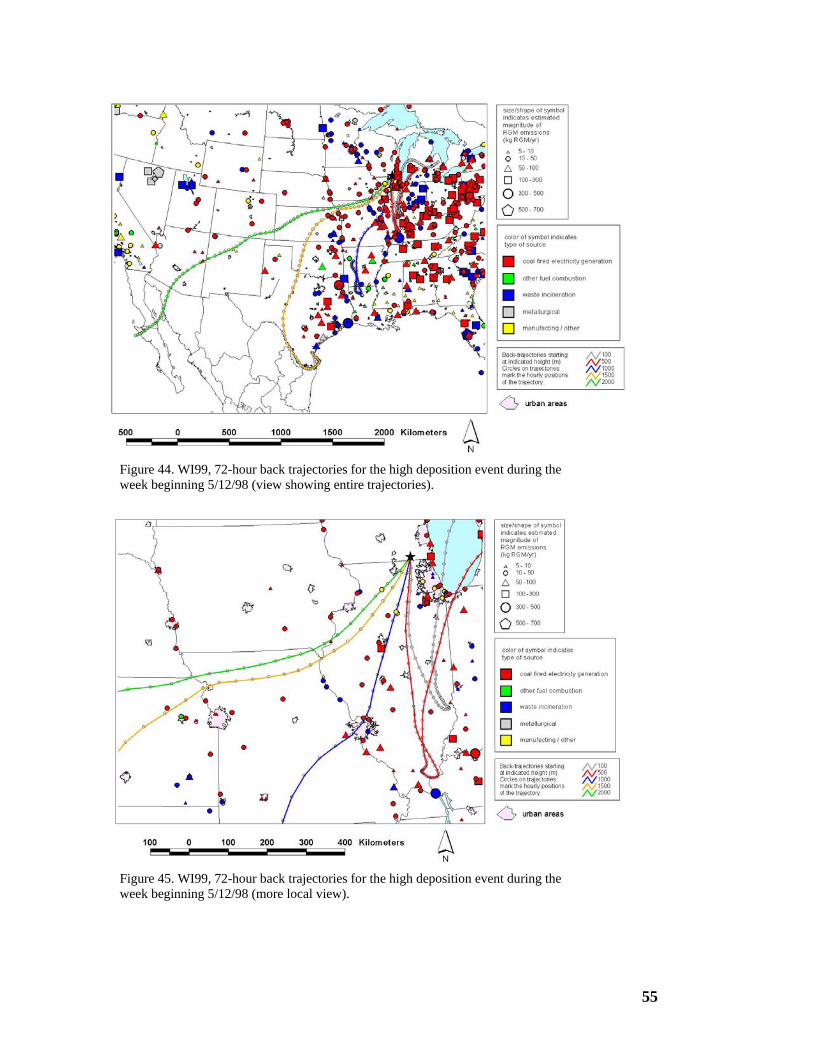
55

Figure 44. WI99, 72-hour back trajectories for the high deposition event during the week beginning 5/12/98 (view showing entire trajectories).

Figure 45. WI99, 72-hour back trajectories for the high deposition event during the week beginning 5/12/98 (more local view).

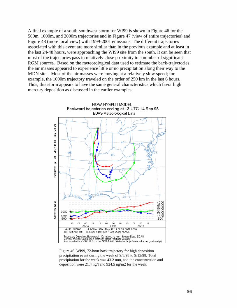
56

A final example of a south-southwest storm for WI99 is shown in Figure 46 for the 500m, 1000m, and 2000m trajectories and in Figure 47 (view of entire trajectories) and Figure 48 (more local view) with 1999-2001 emissions. The different trajectories associated with this event are more similar than in the previous example and at least in the last 24-48 hours, were approaching the WI99 site from the south. It can be seen that most of the trajectories pass in relatively close proximity to a number of significant RGM sources. Based on the meteorological data used to estimate the back-trajectories, the air masses appeared to experience little or no precipitation along their way to the MDN site. Most of the air masses were moving at a relatively slow speed; for example, the 1000m trajectory traveled on the order of 250 km in the last 6 hours. Thus, this storm appears to have the same general characteristics which favor high mercury deposition as discussed in the earlier examples.

Figure 46. WI99, 72-hour back trajectory for high deposition precipitation event during the week of 9/8/98 to 9/15/98. Total precipitation for the week was 43.2 mm, and the concentration and deposition were 21.4 ng/l and 924.5 ug/m2 for the week.

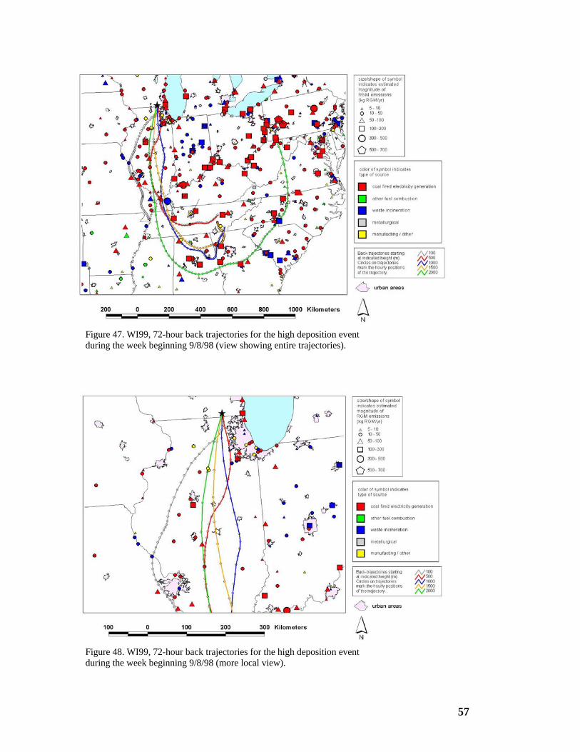
57

Figure 47. WI99, 72-hour back trajectories for the high deposition event during the week beginning 9/8/98 (view showing entire trajectories).

Figure 48. WI99, 72-hour back trajectories for the high deposition event during the week beginning 9/8/98 (more local view).

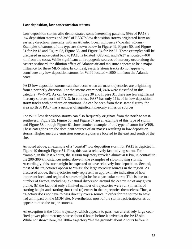
58

Low deposition, low concentration storms Low deposition storms also demonstrated some interesting patterns. 59% of PA13’s low deposition storms and 39% of PA37’s low deposition storms originated from an easterly direction, generally with an Atlantic Ocean influence (“coastal” storms). Examples of storms of this type are shown below in Figure 49, Figure 50, and Figure 51 for PA13 and Figure 52, Figure 53, and Figure 54 for PA37. These examples will be discussed in more detail below. PA13 is located ~320 km, and PA37 is located ~400 km from the coast. While significant anthropogenic sources of mercury occur along the eastern seaboard, the dilution effect of Atlantic air and moisture appears to be a major influence for these MDN sites. In contrast, easterly storm tracks do not appear to contribute any low deposition storms for WI99 located ~1000 km from the Atlantic coast. PA13 low deposition storms can also occur when air mass trajectories are originating from a northerly direction. For the storms examined, 24% were classified in this category (W-NW). As can be seen in Figure 30 and Figure 31, there are few significant mercury sources north of PA13. In contrast, PA37 has only 11% of its low deposition storm tracks with northern orientations. As can be seen from these same figures, the area north of PA37 has a number of significant mercury emission sources. For WI99 low deposition storms can also frequently originate from the north to west-southwest. Figure 55, Figure 56, and Figure 57 are an example of this type of storm, and Figure 58 through Figure 61 show another example of this type of storm for WI99. These categories are the dominant sources of air masses resulting in low deposition storms. Higher mercury emission source regions are located to the east and south of the site. As noted above, an example of a “coastal” low deposition storm for PA13 is depicted in Figure 49 through Figure 51. First, this was a relatively fast-moving storm. For example, in the last 6 hours, the 1000m trajectory traveled almost 400 km, in contrast to the 200-300 km distances noted above in the examples of slow-moving storms. Accordingly, this storm might be expected to have relatively low deposition. Second, most of the trajectories appear to “miss” the large mercury sources in the region. As discussed above, the trajectories only represent an approximate indication of how important local and regional sources might be for a particular storm. This is due to a number of factors, including (a) natural dispersion around the centerline of any given plume, (b) the fact that only a limited number of trajectories were run (in terms of starting height and starting time) and (c) errors in the trajectories themselves. Thus, a trajectory does not have to pass directly over a source in order for the source to have had an impact on the MDN site. Nevertheless, most of the storm back-trajectories do appear to miss the major sources. An exception is the 100m trajectory, which appears to pass near a relatively large coal-fired power plant mercury source about 6 hours before it arrived at the PA13 site. While not shown here, the 100m trajectory “hit the ground” about 2 hours before it

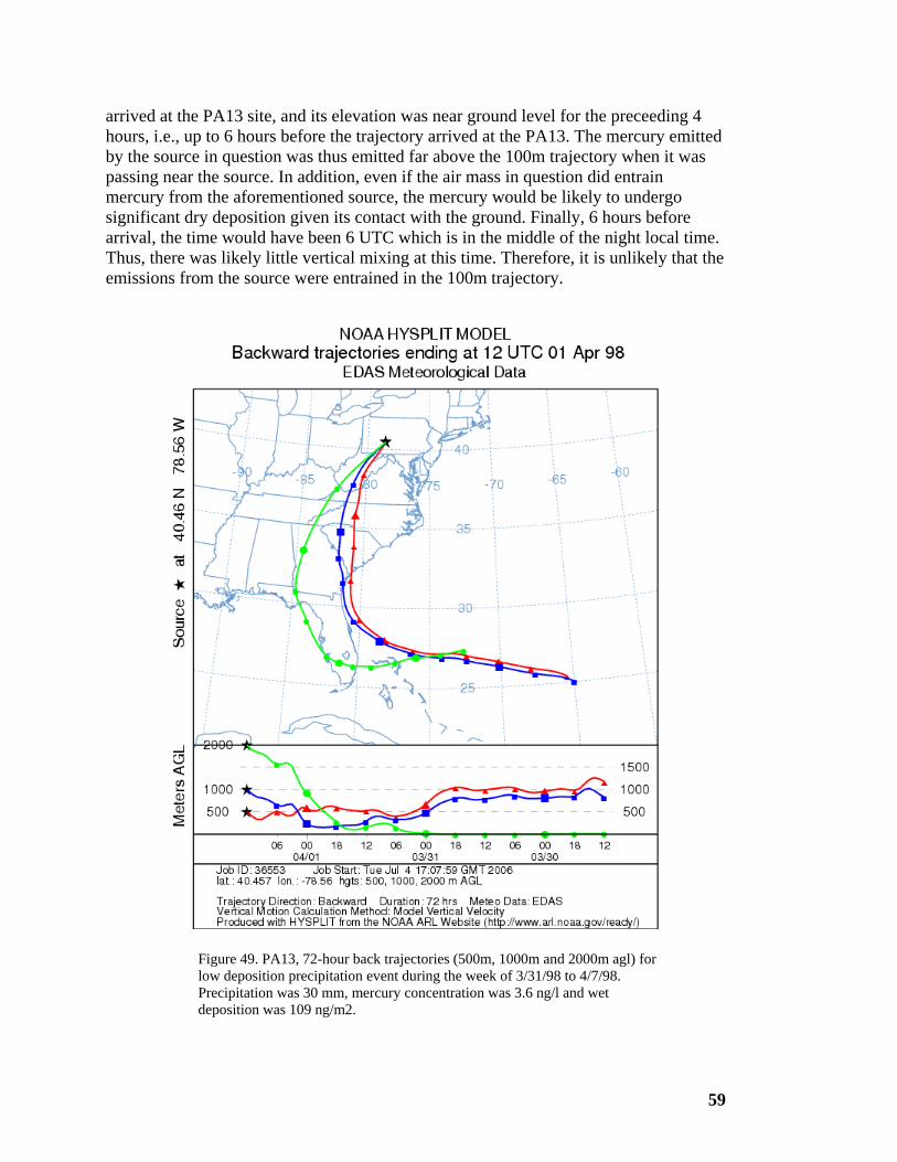
59

arrived at the PA13 site, and its elevation was near ground level for the preceeding 4 hours, i.e., up to 6 hours before the trajectory arrived at the PA13. The mercury emitted by the source in question was thus emitted far above the 100m trajectory when it was passing near the source. In addition, even if the air mass in question did entrain mercury from the aforementioned source, the mercury would be likely to undergo significant dry deposition given its contact with the ground. Finally, 6 hours before arrival, the time would have been 6 UTC which is in the middle of the night local time. Thus, there was likely little vertical mixing at this time. Therefore, it is unlikely that the emissions from the source were entrained in the 100m trajectory.

Figure 49. PA13, 72-hour back trajectories (500m, 1000m and 2000m agl) for low deposition precipitation event during the week of 3/31/98 to 4/7/98. Precipitation was 30 mm, mercury concentration was 3.6 ng/l and wet deposition was 109 ng/m2.

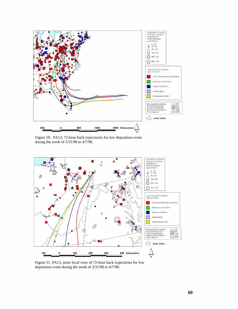
60

Figure 50. PA13, 72-hour back trajectories for low deposition event during the week of 3/31/98 to 4/7/98.

Figure 51. PA13, more local view of 72-hour back trajectories for low deposition event during the week of 3/31/98 to 4/7/98.

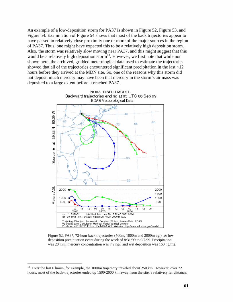
61

An example of a low-deposition storm for PA37 is shown in Figure 52, Figure 53, and Figure 54. Examination of Figure 54 shows that most of the back trajectories appear to have passed in relatively close proximity one or more of the major sources in the region of PA37. Thus, one might have expected this to be a relatively high deposition storm. Also, the storm was relatively slow moving near PA37, and this might suggest that this would be a relatively high deposition storm13. However, we first note that while not shown here, the archived, gridded meterological data used to estimate the trajectories showed that all of the trajectories encountered significant precipitation in the last ~12 hours before they arrived at the MDN site. So, one of the reasons why this storm did not deposit much mercury may have been that mercury in the storm’s air mass was deposited to a large extent before it reached PA37.

Figure 52. PA37, 72-hour back trajectories (500m, 1000m and 2000m agl) for low deposition precipitation event during the week of 8/31/99 to 9/7/99. Precipitation was 20 mm, mercury concentration was 7.9 ng/l and wet deposition was 160 ng/m2.

13. Over the last 6 hours, for example, the 1000m trajectory traveled about 250 km. However, over 72 hours, most of the back-trajectories ended up 1500-2000 km away from the site, a relatively far distance.

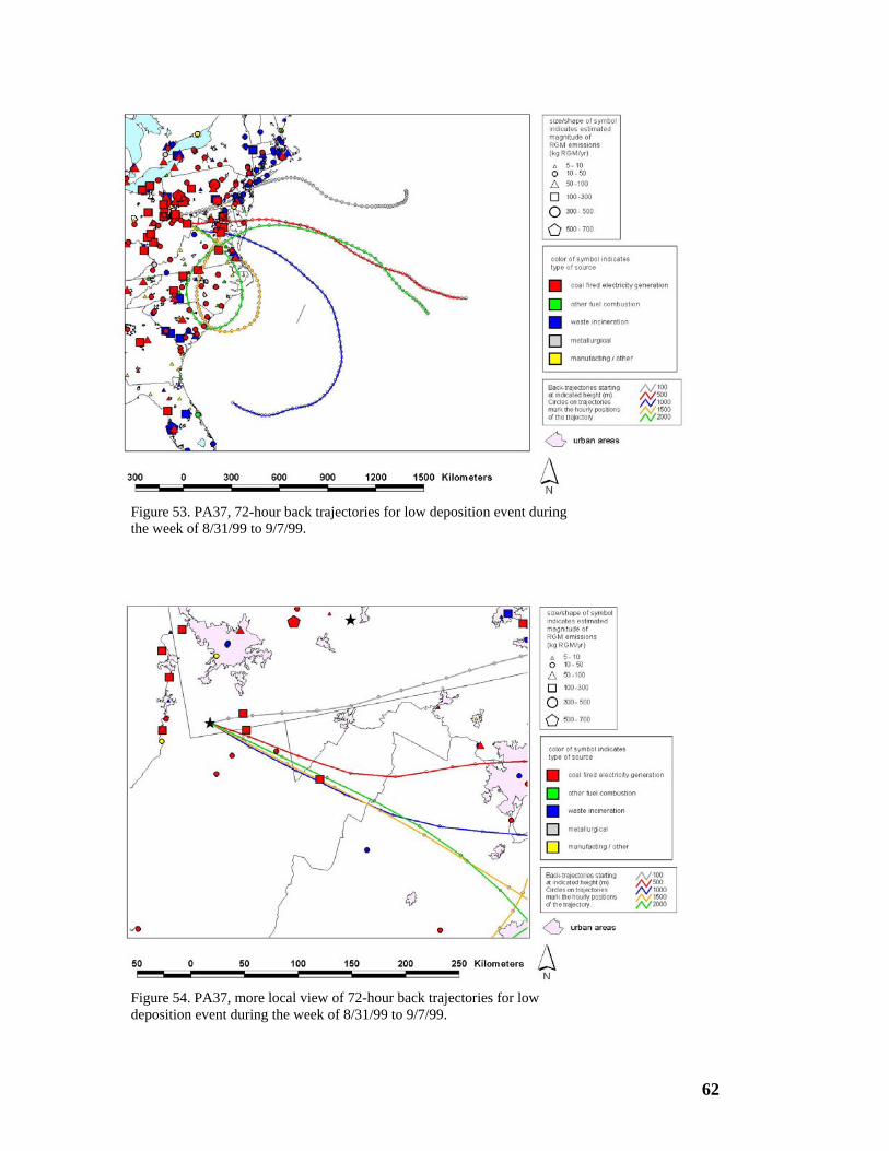
62

Figure 53. PA37, 72-hour back trajectories for low deposition event during the week of 8/31/99 to 9/7/99.

Figure 54. PA37, more local view of 72-hour back trajectories for low deposition event during the week of 8/31/99 to 9/7/99.

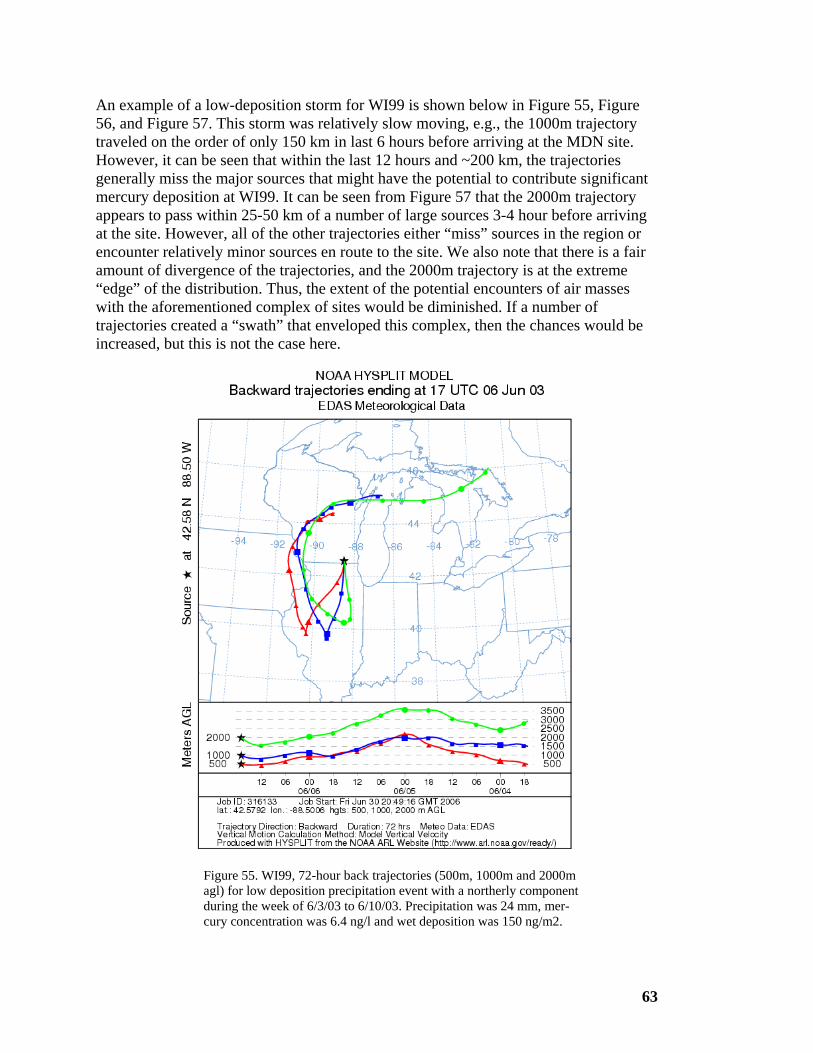
63

An example of a low-deposition storm for WI99 is shown below in Figure 55, Figure 56, and Figure 57. This storm was relatively slow moving, e.g., the 1000m trajectory traveled on the order of only 150 km in last 6 hours before arriving at the MDN site. However, it can be seen that within the last 12 hours and ~200 km, the trajectories generally miss the major sources that might have the potential to contribute significant mercury deposition at WI99. It can be seen from Figure 57 that the 2000m trajectory appears to pass within 25-50 km of a number of large sources 3-4 hour before arriving at the site. However, all of the other trajectories either “miss” sources in the region or encounter relatively minor sources en route to the site. We also note that there is a fair amount of divergence of the trajectories, and the 2000m trajectory is at the extreme “edge” of the distribution. Thus, the extent of the potential encounters of air masses with the aforementioned complex of sites would be diminished. If a number of trajectories created a “swath” that enveloped this complex, then the chances would be increased, but this is not the case here.

Figure 55. WI99, 72-hour back trajectories (500m, 1000m and 2000m agl) for low deposition precipitation event with a northerly component during the week of 6/3/03 to 6/10/03. Precipitation was 24 mm, mer-cury concentration was 6.4 ng/l and wet deposition was 150 ng/m2.

64

Figure 56. WI99, 72-hour back trajectories for low deposition event during the week of 6/3/03 to 6/10/03.

Figure 57. WI99, more local view of 72-hour back trajectories for low deposition event during the week of 6/3/03 to 6/10/03.

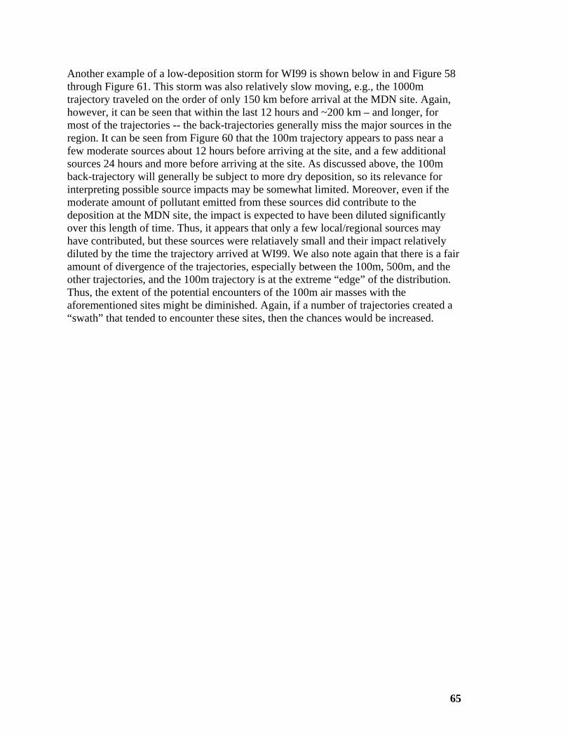
65

Another example of a low-deposition storm for WI99 is shown below in and Figure 58 through Figure 61. This storm was also relatively slow moving, e.g., the 1000m trajectory traveled on the order of only 150 km before arrival at the MDN site. Again, however, it can be seen that within the last 12 hours and ~200 km – and longer, for most of the trajectories -- the back-trajectories generally miss the major sources in the region. It can be seen from Figure 60 that the 100m trajectory appears to pass near a few moderate sources about 12 hours before arriving at the site, and a few additional sources 24 hours and more before arriving at the site. As discussed above, the 100m back-trajectory will generally be subject to more dry deposition, so its relevance for interpreting possible source impacts may be somewhat limited. Moreover, even if the moderate amount of pollutant emitted from these sources did contribute to the deposition at the MDN site, the impact is expected to have been diluted significantly over this length of time. Thus, it appears that only a few local/regional sources may have contributed, but these sources were relatiavely small and their impact relatively diluted by the time the trajectory arrived at WI99. We also note again that there is a fair amount of divergence of the trajectories, especially between the 100m, 500m, and the other trajectories, and the 100m trajectory is at the extreme “edge” of the distribution. Thus, the extent of the potential encounters of the 100m air masses with the aforementioned sites might be diminished. Again, if a number of trajectories created a “swath” that tended to encounter these sites, then the chances would be increased.

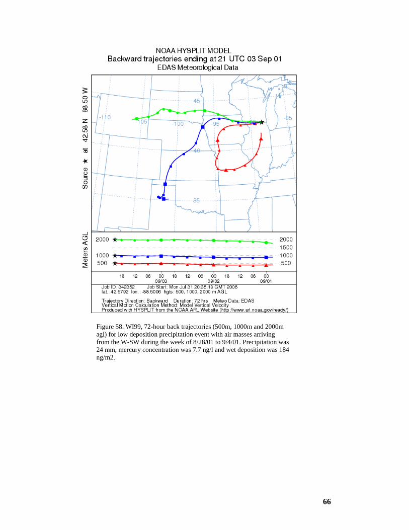
66

Figure 58. WI99, 72-hour back trajectories (500m, 1000m and 2000m agl) for low deposition precipitation event with air masses arriving from the W-SW during the week of 8/28/01 to 9/4/01. Precipitation was 24 mm, mercury concentration was 7.7 ng/l and wet deposition was 184 ng/m2.

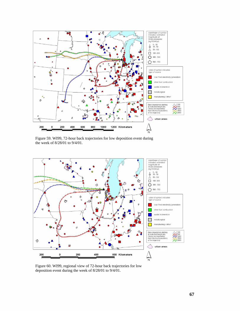
67

Figure 59. WI99, 72-hour back trajectories for low deposition event during the week of 8/28/01 to 9/4/01.

Figure 60. WI99, regional view of 72-hour back trajectories for low deposition event during the week of 8/28/01 to 9/4/01.

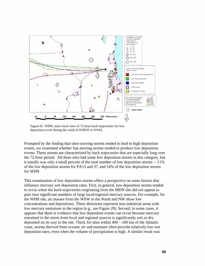
68

Figure 61. WI99, more local view of 72-hour back trajectories for low deposition event during the week of 8/28/01 to 9/4/01.

Prompted by the finding that slow-moving storms tended to lead to high deposition events, we examined whether fast moving storms tended to produce low deposition events. These storms are characterized by back trajectories that are especially long over the 72-hour period. All three sites had some low deposition storms in this category, but it usually was only a small percent of the total number of low deposition storms -- 11% of the low deposition storms for PA13 and 37, and 14% of the low deposition storms for WI99. This examination of low deposition storms offers a perspective on some factors that influence mercury wet deposition rates. First, in general, low deposition storms tended to occur when the back-trajectories originating from the MDN site did not appear to pass near significant numbers of large local/regional mercury sources. For example, for the WI99 site, air masses from the WSW to the North and NW show low concentrations and depositions. These directions represent non-industrial areas with low mercury emissions in the region (e.g., see Figure 29). Second, in some cases, it appears that there is evidence that low deposition events can occur because mercury entrained in the storm from local and regional sources is significantly wet or dry deposited on its way to the site. Third, for sites within 400 – 500 km of the Atlantic coast, storms derived from oceanic air and moisture often provide relatively low wet deposition rates, even when the volume of precipitation is high. A similar result was

69

found for other pollutant species, NO3- and SO4

= concentration and deposition, at the Hubbard Brook Experimental Forest in New Hampshire (Likens et al. 1990). Conclusions In the random coefficient model analyses conducted here, we found that as a group, long-term MDN sites in the northeastern quadrant of the U.S. (and southeastern Canada) show a statistically significant decline in mercury wet deposition and mercury precipitation concentration, but that as a group, sites in the southeastern quadrant do not show a stastically significant trend. The difference in the two regions appears to be consistent with the limited available information on regional emissions changes that we could assemble. These emissions inventory data suggest that emissions declines in the northeastern region were greater than emissions declines in the southeastern region. Natural sources and other anthropogenic source regions certainly also have an impact, as do factors related to atmospheric transport and transformation of mercury. Based on the above results we have hypothesized that while U.S. and Canadian mercury emissions have decreased, this decrease has been offset by the impact of increasing emissions from Asia (for example China and India). For the group of northeastern sites, the decline in local/regional emissions was larger than this offset, and the overall deposition observed at this group of sites decreased. In the southeastern group, the decrease in local/regional emission was smaller and its impact was comparable to the impact of increasing emissions elsewhere. In carrying out this analysis, we encountered a significant problem related to the availability of emissions inventory data. The lack of temporal resolution and the lack of data more recent than 1999 presented a major challenge. In essence, there is no continuous record of mercury emissions over the time period that MDN has operated at long-term sites, even for significant point sources. Therefore it is exceedingly difficult to analyze the changes in deposition in relation to whatever changes in emissions that might have occurred. A new emissions inventory for the year 2002 is expected to come out shortly but details at the state level are still not available. Improvements in the accuracy of the record would help in better understanding the impacts of local/regional emission changes, and their impact on deposition Our somewhat preliminary and qualitative analysis of storm back trajectories at three MDN sites suggests that high deposition storms can occur when the air masses arriving at the site entrained emissions from large local and regional sources. This interpretation of these storms and back-trajectories is fraught with difficulty, but in general, the data appear to show that the local and regional sources can contribute significantly to deposition at MDN sites. Low deposition storms at the two northeastern U.S. sites examined (PA13 and PA37) were often “coastal” in origin. For the site in the midwest (WI99), storms from the west and north – areas with few major mercury sources -- often had low concentrations and depositions.

70

Combining the review of the literature and various analyses carried out here, we conclude that there is evidence supporting the importance of local/ regional anthropogenic emissions in contributing to the deposition observed at MDN sites.

71

References: Bindler R., C. Olofsson, I. Renberg and W. Frech. 2001. Temporal trends in mercury

accumulation in lake sediments in Sweden. Water, Air and Soil Pollution: Focus 1:343-355.

Browne, C.L. and S.C. Fang 1978. Uptake of mercury vapor by wheat. Plant

Physiology 61:430-433. Bullock, O.R., and K.A. Brehme (2002). Atmospheric mercury simulation using the

CMAQ model: formulation description and analysis of wet deposition results. Atmos. Environ 36: 2135-2146.

Calvert, J. G. and S.E. Lindberg, 2005. Mechanisms of mercury removal by O3 and OH

in the atmosphere. Atmos. Environ. 39:3355-3367. Cohen M., R. Artz, R. Draxler, P. Miller, L. Poissant, D. Niemi, D. Ratte, M.

Deslauriers, R. Duval, R. Laurin, J. Slotnick, T. Nettesheim and J. McDonald, 2004. Modeling the atmospheric transport and deposition of mercury to the Great Lakes. Environ. Research 95:247-265.

Engstrom, D.R. and E.B. Swain, 1997. Recent declines in atmospheric mercury

deposition in the Upper Midwest. Environ. Sci. Technol. 31:960-967. EPRI (Electric Power Research Institute) 2004. Atmospheric Mercury Research

Update. Final Report. Available at: http://www.epa.gov/mercury/pdfs/OAR-2002-0056-2589.pdf

Glass, G. E. and J.A. Sorensen. 1999. Six-year trend (1990-1995) of wet mercury

deposition in the upper Midwest, USA. Environ. Sci. Technol. 33:3303-3312 Goodsite, M.E., J.M.C. Plane and H. Skov, 2004. A theoretical study of the oxidation

of Hgo to HgBr2 in the troposphere. Environ. Sci. Technol. 38:1772-1776. Guentzel, J. L., W.M. Landing, G.A. Gill and C.C. Pollman 2001. Processes

influencing rainfall deposition of mercury in Florida. Environ. Sci. Technol. 35:863-873

Han, Y-I, T.M. Holsen, S-O Lai, P.K. Hopke, A-M Yi, W. Liu, J. Pagano, L. Falanga,

M. Milligan and C. Andolina. 2004. Atmospheric gaseous mercury concentrations in New York State: relationships with meteorloical data and other pollutants. Atmos. Environ. 38:6431-6446.

72

Hedgecock, I., Pirrone, N. (2001). Mercury and photochemistry in the marine boundary layer-modeling studies suggest the in situ production of reactive gas phase mercury. Atmospheric Environment 35, 3055-3062.

Hintelmann, H., R. Harris, A. Heyes, J.P. Hurley, C.A. Kelly, D.P. Krabbenhoft,

S.Lindberg, J.W.M. Rudd, K.J. Scott and V.L. St. Louis, 2002. Reactivity and mobility of new and old mercury deposition in a boreal forest ecosystem during the first year of the METALLICUS study. Environ. Sci. Technol. 36:5034-5040.

Jaffe, D., P. Swartzendruber, E. Prestbo, W. Hafner and P. Weiss (2005). Long-Range

Transport of Mercury to the U.S. Presented at NADP 2005 Technical Committee Meeting. Sept. 2005. Jackson Hole, WY.

Keeler, G.J. and J.T. Dvonch, 2004. Atmospheric Mercury: A Decade of Observation

in the Great Lakes in N. Pirrone and K. Mahaffey (eds.) Dynamics of Mercury Pollution on Regional and Global Scales: Atmospheric Processes and Human Exposures around the World: Kluwer Ltd.

Keeler, G.J., L.E. Gratz and K. Al-Wali, 2005. Long-term atmospheric mercury wet

deposition at Underhill, Vermont. Ecotoxicology 14:71-83. Keeler, G. and S-J Yoo, 2003. Mercury deposition and atmospheric concentrations in

New England. Final REMAP Report. Northeast States for Coordinated Air Use Management, Boston, MA. 44pp.

Keeler, G.J., Landis, M.S., Norris, G.A., Christianson, E.M., Dvonch, J.T. (2006).

Sources of Mercury Wet Deposition in Eastern Ohio, USA. Environ. Sci. Technol.2006, 40,5874-5881

Landis M.S. A.F. Vette and G.J. Keeler. 2002. Atmospheric mercury in the Lake

Michigan basin: Influence of the Chicago/Gary urban area. Environ. Sci. Technol. 36:4508-4517.

Landis, M.S. and G.J. Keeler, 2002. Atmospheric mercury deposition to Lake Michigan

during the Lake Michigan Mass Balance Study. Environ. Sci and Tech 33:2067-2079.

Laurier, F., Mason, R., Whalin, L., Kato, S. (2003). Reactive gaseous mercury

formation in the North Pacific Ocean’s marine boundary layer: A potential role of halogen chemistry. J. Geophysical Research 108, D-17, 4529.

Likens, G.E., L.O. Hedin and T.J. Butler, 1990. Some long-term precipitation

chemistry patterns at the Hubbard Brook Experimental Forest: extremes and averages. Verh. Internat. Verein. Limnol. 24:128-135.

73

Lin, C.J. and S.O. Pehkonen 1999. The Chemistry of atmospheric mercury: a review. Atmos Environ. 33:2067-2079.

Lindberg, S. E.; Brooks, S.; Lin, C.-J.; Scott, K. J.; Landis, M. S.; Stevens, R. K.;

Goodsite, M.; Richter, A. (2002). Dynamic Oxidation of Gaseous Mercury in the Arctic Troposphere at Polar Sunrise. Environ. Sci. Technol. 36, 1245-1256

Lindqvist, O., K. Johansson, A. Astrup, A. Anderson, L. Bringmark, G. Hovsenius, A.

Iverfeldt, M. Meili and B. Timm, 1991. Mercury in the Swedish environment. Water Air Soil Pollut. 55:1-261.

Littell, R. C., Millikan, G.A., Stroup, W.W. and Wolfinger, R.D., 1996. SAS System

for Mixed Models. SAS Institute Inc., NC, USA. 633 pp. Lorey P. and C.T. Driscoll. 1999. Historical trends of mercury deposition in

Adirondack lakes. Environ. Sci. Technol. 33:718-722. Mason R.P., N.M. Lawson and G.R. Sheu 2000 Annual and seasonal trends in mercury

deposition in Maryland. Atmos. Environ. 34:1691-1701 Mason, R.P., W.F. Fitzgerald and F.M. Morel, 1994. The biogeochemical cycling of

elemental mercury: anthropogenic influences. Geochimica et Cosmochimica Acta 58:3191-3198.

MDN (Mercury Deposition Network), 2006. Website: http://nadp.sws.uiuc.edu/mdn/ Mosbaek, H., J.C. Tjell, T. Sevel 1988. Plant uptake of airborne mercury in background

areas. Chemosphere 17:1227-1236. Norton S.A., G.C. Evans and J.S. Kahl, 1997. Comparison of Hg and Pb fluxes to

hummocks and hollows of ombrotrophic Big Heath Bog and to nearby Sargent Mt. Pond, Maine, USA. Water, Air Soil Pollut. 100:271-286.

Pacyna, J., Wilson, S., and Steenhuisen, F., 2005. Spatially distributed inventories of

global anthropogenic emissions of mercury to the atmosphere. http://www.amap.no/Resources/HgEmissions/HgInventoryMain.html

Pacyna EG, Pacyna JM, Steenhuisen F, Wilson S (2006). Global anthropogenic

mercury emission inventory for 2000. Atmos. Environ. 40 (22): 4048-4063. Pirrone, N., G.J. Keeler and J.O. Nriagu, 1996. Regional differences in worldwide

emissions of mercury to the atmosphere. Atmos. Environ. 30:2981-2987. Pirrone, N., I. Allegrini. G.J. Keeler, J.O. Nriagu, R. Rossmann and J.A. Robbins.

1998. Historical atmospheric mercury emissions and depositions in North

74

America compared to mercury accumulations in sedimentary records. Atmos. Environ. 32:929-940.

Prestbo, E., Leutner, J., and Pollman, C. (2006). Abrupt Decrease in Mercury Wet-

deposition Concentration and Annual Flux in Seattle, Washington Due to Emission Point-source Changes. Presented at the Eighth International Conference on Mercury as a Global Pollutant, August 6-11, 2006, Madison Wisconsin.

Rea. A.W., S.E. Lindberg and G.J. Keeler 2001. Dry deposition and foliar leaching of

mercury and selected trace elements in deciduous forest throughfall. Atmos. Environ. 35:3453-3462

Raudenbush, S.W. and Bryk, A.S., 2002. Hierarchical Linear Models: Applications and

Data Analysis Methods. Second Edition. Newbury Park, CA: Sage Publications. Rosenbaum, A., D. Axelrad, T. Woodruff, Y. Wei, M. Ligocki, J. Cohen (1999a).

National estimates of outdoor air toxics concentrations. J Air Waste Management Assoc. 49: 1138-1152.

Rosenbaum, A., M. Ligocki, Y. Wei (1999b). Modeling Cumulative Outdoor

Concentrations of Hazardous Air Pollutants: Revised Final Report. Systems Applications International, Inc., San Rafael, CA. As cited in Rosenbaum et al., 1999a.

Round, M. and M. Irvine, 2004. Update on Mercury Inventory and Modeling Project.

Presentaion at the May 27, 2004 Symposium on Mercury Contamination in the Northeast.

Ryan, P., H. Hafner and S. Brown, 2003. Deposition of air pollutants to Casco Bay.

Final Report. STI-902150-2209-FR. Casco Bay Estuary Project. Portland, ME USA. 80 pp. with appendices.

Schuster, P.F., D.P. Krabbenhoft, D.L. Naftz, L.D. Cecil, M.L. Olson, J.F. Dewild,

D.D. Suson, J.R. Green and M.L. Abbott, 2002. Atmospheric mercury deposition during the last 270 years: a glacial ice core record of natural and anthropogenic sources.Environ. Sci. Technol. 36:2303-2310.

Schroeder W. H. and J Munthe. 1998. Atmospheric Mercury – an overview. Atmos.

Environ. 32:809-822. Seigneur, C., Karamchandani, P., Lohman, K., Vijayaraghavan, K. (2001). Multiscale

modeling of the atmospheric fate and transport of mercury. J. Geophysical Res. 106 (D21), 27795-27809.

75

Seigneur, C.K., K. Lohman, K. Vijayaraghavan and R. Shia, 2003. Contributions of global and regional sources to mercury deposition in New York State. Environ. Pollut. 123:365-373.

Seigneur C., K. Vijayaraghavan, K. Lochman, P. Karamchandani and C. Scott. 2004.

Gobal source attribution for mercury deposition in the United States. Environ. Sci.Technol. 38:555-569.

Singer, Judith D., 1998. Using SAS PROC MIXED to Fit Multilevel Models,

Hierarchial Models, and Individual Growth Models. Journal of Educational and Behavioral Statistics 23, 323-355.

Slemr, F.and E. Langer 1992. Increase in global atmospheric concentrations of mercury inferred from measurements over the Atlantic Ocean. Nature 1355(6359):434.

Slemr, F., W. Junkermann, R.W.H. Schmidt and R. Sladkovic. 1995. Indication of

change in global and regional trends of mercury concentrations. Geophys. Res. Letters 22:2143-2146.

Snijders, T.and Bosker, R., 1999. Multilevel Analysis. An Introduction to Basic and

Advanced Modeling. Thousand Oakes, CA: Sage Publications. Sommar, J.K., K. Gardfeldt, D. Stromberg ans X. Feng. 2001. A kinetic study of the

gas-phase reaction between the hydroxyl radical and atomic mercury. Atmos. Environ. 35:3049-3054.

Stevens, R., J. Shrock, J. Bowser and W. Mayhew, 2000. Technical Report EPA

600/R-00/102. U.S. EPA National Exposure Research Laboratory; Research Triangle Park, NC. (in Landis and Keeler, 2002)

Streets et al., 2005, Anthropogenic mercury emissions in China, Atmospheric

Environment 39, 7789-7806. U.S. EPA (2006). Graph presented by EPA at:

http://www.epa.gov/mercury/control_emissions/emissions.htm U.S. EPA (2005a). Personal communication, U.S. EPA. These data are based on the

1990 National Toxics Inventory (NTI) and the 1999 National Emissions Inventory (NEI) for Hazardous Air Pollutants (HAPs). The data are similar to those presented on the EPA’s mercury website at: http://www.epa.gov/mercury/control_emissions/emissions.htm

U.S. EPA (2005b). Technical Support Document for the Final Clean Air Mercury Rule.

Air Quality Modeling. Office of Air Quality Planning and Standards. Research Triangle Park, NC, March. http://www.epa.gov/ttn/atw/utility/aqm_oar-2002-0056-6130.pdf

76

U.S. EPA (2005c). Technical Support Document: Methodology Used to Generate

Deposition, Fish Tissue Methylmercury Concentrations, and Exposure for Determining Effectiveness of Utility Emission Controls. Analysis of Mercury from Electricity Generating Units. Office of Air Quality Planning and Standards. Research Triangle Park, NC. Available at: http://www.epa.gov/ttn/atw/utility/eff_fnl_tsd-031705_corr_oar-2002-0056-6301.pdf

U.S. EPA (1997). Mercury Study Report to Congress. Office of Air Quality Planning

and Standards and Office of Research and Development. Van Ardsdale, A., J. Weiss, G. Keeler, E. Miller, G. Boulet, R. Brulotte and L.

Poissant, 2005. Patterns of mercury deposition and concentration in Northeastern North America (1996-2002). Ecotoxicology 14:37-52

Wilson SJ, Steenhuisen F, Pacyna JM, Pacyna EG (2006). Mapping the spatial

distribution of global anthropogenic mercury atmospheric emission inventories. Atmos. Environ. 40 (24): 4621-4632.

Zhang, M. Q., Y.C. Zhu and R.W.Deng. 2002. Evaluation of mercury emissions to the

atmosphere from coal combustion, China. Ambio 31:482-484.

77

Appendix I

Annual Concentration and

Deposition for Sites used in

Random Coefficiant

Models

Region Site Site type Year Hg Concentration Hg Deposition Precipitation ng/l ug/m2 cm

6 IL11 n=north 1999 10 9 90.0 6 IL11 n 2000 11.6 9.6 82.8 6 IL11 n 2001 10.5 9 85.7 6 IL11 n 2002 11 9.6 87.3 6 IL11 n 2003 10.8 9.4 87.0 6 IL11 n 2004 10.4 10.1 97.1 6 IL11 n 2005 9.7 8.5 87.3 3 ME02 n 1998 6.5 6.9 106.2 3 ME02 n 1999 6.3 6.9 109.5 3 ME02 n 2000 6.4 6.9 107.8 3 ME02 n 2001 6.6 4.8 72.7 3 ME02 n 2002 5.1 4.9 96.1 3 ME02 n 2003 8.5 9.4 110.6 3 ME02 n 2004 6.2 6.2 100.0 3 ME02 n 2005 5 7.2 145.3 3 ME09 n 1998 6 6.8 113.3 3 ME09 n 1999 5.5 6.9 125.5 3 ME09 n 2000 5.1 5.2 102.0 3 ME09 n 2001 6.2 4 64.5 3 ME09 n 2002 4.8 4.1 85.4 3 ME09 n 2003 6 6.4 106.7 3 ME09 n 2004 7.2 6.5 90.3 3 ME09 n 2005 4.4 6.3 140.8 3 ME96 n 1998 8.6 11 127.9 3 ME96 n 1999 7.3 8.4 115.1 3 ME96 n 2000 6.6 7.9 119.7 3 ME96 n 2001 6.9 4.9 71.0 3 ME96 n 2002 5.1 5.7 111.8 3 ME96 n 2003 6.8 7.2 105.9 3 ME96 n 2004 10.2 10.2 100.0 3 ME96 n 2005 4.9 7.9 158.1 3 ME98 n 1998 6.1 9 147.5 3 ME98 n 1999 6.1 8 131.1 3 ME98 n 2000 7 8.7 124.3 3 ME98 n 2001 8 5.3 66.3 3 ME98 n 2002 5.1 8 156.9 3 ME98 n 2003 5.6 7.2 128.6

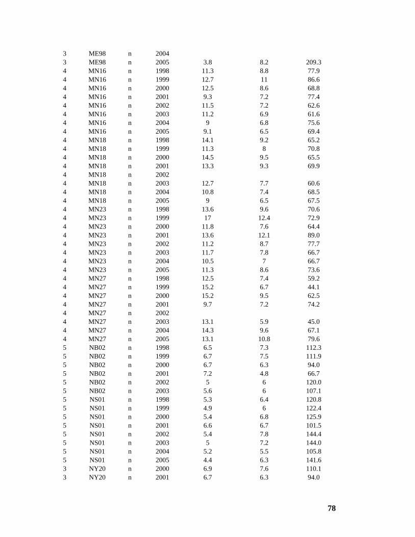
78

3 ME98 n 2004 3 ME98 n 2005 3.8 8.2 209.3 4 MN16 n 1998 11.3 8.8 77.9 4 MN16 n 1999 12.7 11 86.6 4 MN16 n 2000 12.5 8.6 68.8 4 MN16 n 2001 9.3 7.2 77.4 4 MN16 n 2002 11.5 7.2 62.6 4 MN16 n 2003 11.2 6.9 61.6 4 MN16 n 2004 9 6.8 75.6 4 MN16 n 2005 9.1 6.5 69.4 4 MN18 n 1998 14.1 9.2 65.2 4 MN18 n 1999 11.3 8 70.8 4 MN18 n 2000 14.5 9.5 65.5 4 MN18 n 2001 13.3 9.3 69.9 4 MN18 n 2002 4 MN18 n 2003 12.7 7.7 60.6 4 MN18 n 2004 10.8 7.4 68.5 4 MN18 n 2005 9 6.5 67.5 4 MN23 n 1998 13.6 9.6 70.6 4 MN23 n 1999 17 12.4 72.9 4 MN23 n 2000 11.8 7.6 64.4 4 MN23 n 2001 13.6 12.1 89.0 4 MN23 n 2002 11.2 8.7 77.7 4 MN23 n 2003 11.7 7.8 66.7 4 MN23 n 2004 10.5 7 66.7 4 MN23 n 2005 11.3 8.6 73.6 4 MN27 n 1998 12.5 7.4 59.2 4 MN27 n 1999 15.2 6.7 44.1 4 MN27 n 2000 15.2 9.5 62.5 4 MN27 n 2001 9.7 7.2 74.2 4 MN27 n 2002 4 MN27 n 2003 13.1 5.9 45.0 4 MN27 n 2004 14.3 9.6 67.1 4 MN27 n 2005 13.1 10.8 79.6 5 NB02 n 1998 6.5 7.3 112.3 5 NB02 n 1999 6.7 7.5 111.9 5 NB02 n 2000 6.7 6.3 94.0 5 NB02 n 2001 7.2 4.8 66.7 5 NB02 n 2002 5 6 120.0 5 NB02 n 2003 5.6 6 107.1 5 NS01 n 1998 5.3 6.4 120.8 5 NS01 n 1999 4.9 6 122.4 5 NS01 n 2000 5.4 6.8 125.9 5 NS01 n 2001 6.6 6.7 101.5 5 NS01 n 2002 5.4 7.8 144.4 5 NS01 n 2003 5 7.2 144.0 5 NS01 n 2004 5.2 5.5 105.8 5 NS01 n 2005 4.4 6.3 141.6 3 NY20 n 2000 6.9 7.6 110.1 3 NY20 n 2001 6.7 6.3 94.0

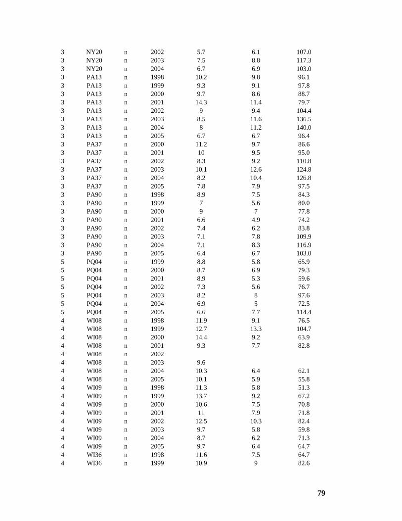
79

3 NY20 n 2002 5.7 6.1 107.0 3 NY20 n 2003 7.5 8.8 117.3 3 NY20 n 2004 6.7 6.9 103.0 3 PA13 n 1998 10.2 9.8 96.1 3 PA13 n 1999 9.3 9.1 97.8 3 PA13 n 2000 9.7 8.6 88.7 3 PA13 n 2001 14.3 11.4 79.7 3 PA13 n 2002 9 9.4 104.4 3 PA13 n 2003 8.5 11.6 136.5 3 PA13 n 2004 8 11.2 140.0 3 PA13 n 2005 6.7 6.7 96.4 3 PA37 n 2000 11.2 9.7 86.6 3 PA37 n 2001 10 9.5 95.0 3 PA37 n 2002 8.3 9.2 110.8 3 PA37 n 2003 10.1 12.6 124.8 3 PA37 n 2004 8.2 10.4 126.8 3 PA37 n 2005 7.8 7.9 97.5 3 PA90 n 1998 8.9 7.5 84.3 3 PA90 n 1999 7 5.6 80.0 3 PA90 n 2000 9 7 77.8 3 PA90 n 2001 6.6 4.9 74.2 3 PA90 n 2002 7.4 6.2 83.8 3 PA90 n 2003 7.1 7.8 109.9 3 PA90 n 2004 7.1 8.3 116.9 3 PA90 n 2005 6.4 6.7 103.0 5 PQ04 n 1999 8.8 5.8 65.9 5 PQ04 n 2000 8.7 6.9 79.3 5 PQ04 n 2001 8.9 5.3 59.6 5 PQ04 n 2002 7.3 5.6 76.7 5 PQ04 n 2003 8.2 8 97.6 5 PQ04 n 2004 6.9 5 72.5 5 PQ04 n 2005 6.6 7.7 114.4 4 WI08 n 1998 11.9 9.1 76.5 4 WI08 n 1999 12.7 13.3 104.7 4 WI08 n 2000 14.4 9.2 63.9 4 WI08 n 2001 9.3 7.7 82.8 4 WI08 n 2002 4 WI08 n 2003 9.6 4 WI08 n 2004 10.3 6.4 62.1 4 WI08 n 2005 10.1 5.9 55.8 4 WI09 n 1998 11.3 5.8 51.3 4 WI09 n 1999 13.7 9.2 67.2 4 WI09 n 2000 10.6 7.5 70.8 4 WI09 n 2001 11 7.9 71.8 4 WI09 n 2002 12.5 10.3 82.4 4 WI09 n 2003 9.7 5.8 59.8 4 WI09 n 2004 8.7 6.2 71.3 4 WI09 n 2005 9.7 6.4 64.7 4 WI36 n 1998 11.6 7.5 64.7 4 WI36 n 1999 10.9 9 82.6

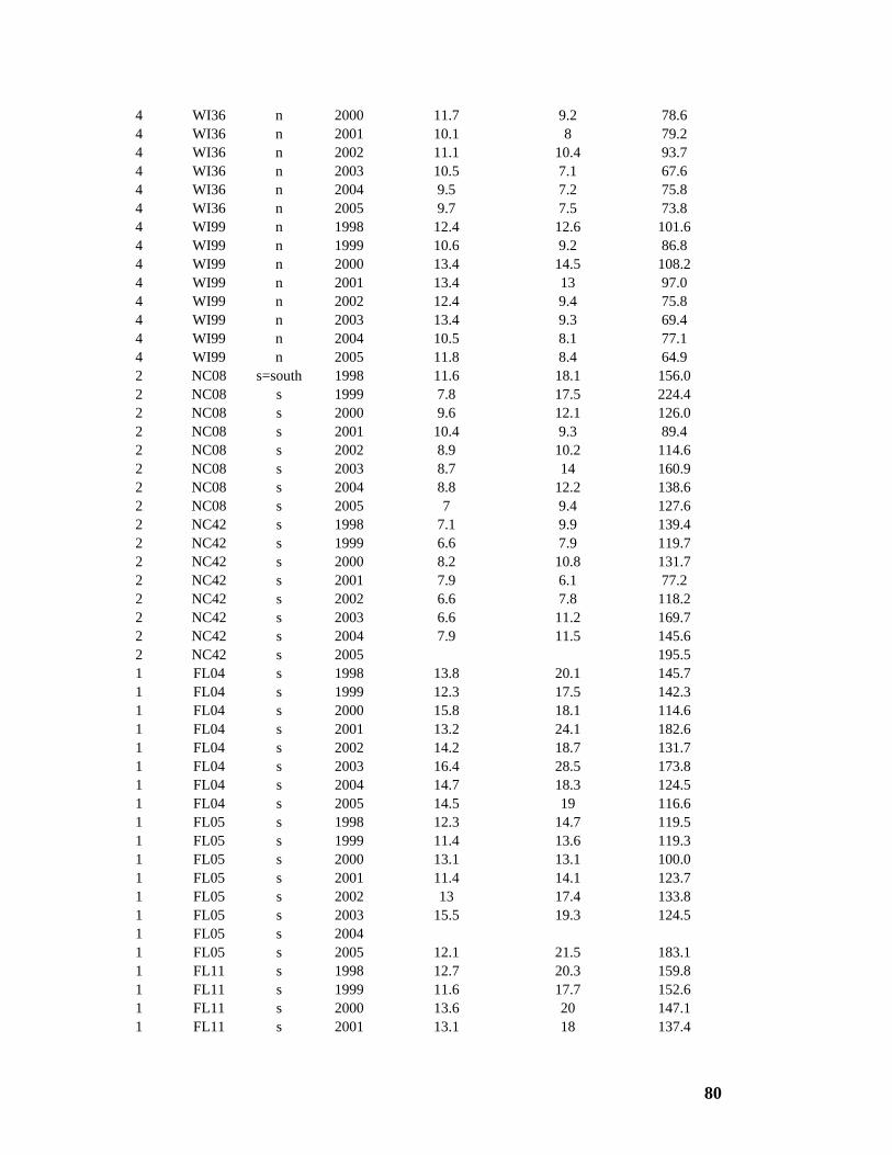
80

4 WI36 n 2000 11.7 9.2 78.6 4 WI36 n 2001 10.1 8 79.2 4 WI36 n 2002 11.1 10.4 93.7 4 WI36 n 2003 10.5 7.1 67.6 4 WI36 n 2004 9.5 7.2 75.8 4 WI36 n 2005 9.7 7.5 73.8 4 WI99 n 1998 12.4 12.6 101.6 4 WI99 n 1999 10.6 9.2 86.8 4 WI99 n 2000 13.4 14.5 108.2 4 WI99 n 2001 13.4 13 97.0 4 WI99 n 2002 12.4 9.4 75.8 4 WI99 n 2003 13.4 9.3 69.4 4 WI99 n 2004 10.5 8.1 77.1 4 WI99 n 2005 11.8 8.4 64.9 2 NC08 s=south 1998 11.6 18.1 156.0 2 NC08 s 1999 7.8 17.5 224.4 2 NC08 s 2000 9.6 12.1 126.0 2 NC08 s 2001 10.4 9.3 89.4 2 NC08 s 2002 8.9 10.2 114.6 2 NC08 s 2003 8.7 14 160.9 2 NC08 s 2004 8.8 12.2 138.6 2 NC08 s 2005 7 9.4 127.6 2 NC42 s 1998 7.1 9.9 139.4 2 NC42 s 1999 6.6 7.9 119.7 2 NC42 s 2000 8.2 10.8 131.7 2 NC42 s 2001 7.9 6.1 77.2 2 NC42 s 2002 6.6 7.8 118.2 2 NC42 s 2003 6.6 11.2 169.7 2 NC42 s 2004 7.9 11.5 145.6 2 NC42 s 2005 195.5 1 FL04 s 1998 13.8 20.1 145.7 1 FL04 s 1999 12.3 17.5 142.3 1 FL04 s 2000 15.8 18.1 114.6 1 FL04 s 2001 13.2 24.1 182.6 1 FL04 s 2002 14.2 18.7 131.7 1 FL04 s 2003 16.4 28.5 173.8 1 FL04 s 2004 14.7 18.3 124.5 1 FL04 s 2005 14.5 19 116.6 1 FL05 s 1998 12.3 14.7 119.5 1 FL05 s 1999 11.4 13.6 119.3 1 FL05 s 2000 13.1 13.1 100.0 1 FL05 s 2001 11.4 14.1 123.7 1 FL05 s 2002 13 17.4 133.8 1 FL05 s 2003 15.5 19.3 124.5 1 FL05 s 2004 1 FL05 s 2005 12.1 21.5 183.1 1 FL11 s 1998 12.7 20.3 159.8 1 FL11 s 1999 11.6 17.7 152.6 1 FL11 s 2000 13.6 20 147.1 1 FL11 s 2001 13.1 18 137.4

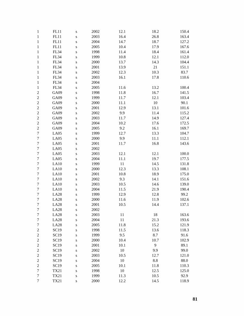
81

1 FL11 s 2002 12.1 18.2 150.4 1 FL11 s 2003 16.4 26.8 163.4 1 FL11 s 2004 14.7 18.7 127.2 1 FL11 s 2005 10.4 17.9 167.6 1 FL34 s 1998 11.4 18.4 161.4 1 FL34 s 1999 10.8 12.1 112.0 1 FL34 s 2000 13.7 14.3 104.4 1 FL34 s 2001 13.9 21 151.1 1 FL34 s 2002 12.3 10.3 83.7 1 FL34 s 2003 16.1 17.8 110.6 1 FL34 s 2004 1 FL34 s 2005 11.6 13.2 100.4 2 GA09 s 1998 11.8 16.7 141.5 2 GA09 s 1999 11.7 12.1 103.4 2 GA09 s 2000 11.1 10 90.1 2 GA09 s 2001 12.9 13.1 101.6 2 GA09 s 2002 9.9 11.4 115.2 2 GA09 s 2003 11.7 14.9 127.4 2 GA09 s 2004 10.2 17.6 172.5 2 GA09 s 2005 9.2 16.1 169.7 7 LA05 s 1999 12.7 13.3 104.7 7 LA05 s 2000 9.9 11.1 112.1 7 LA05 s 2001 11.7 16.8 143.6 7 LA05 s 2002 7 LA05 s 2003 12.1 12.1 100.0 7 LA05 s 2004 11.1 19.7 177.5 7 LA10 s 1999 11 14.5 131.8 7 LA10 s 2000 12.3 13.3 108.1 7 LA10 s 2001 10.8 18.9 175.0 7 LA10 s 2002 9.3 14.1 151.6 7 LA10 s 2003 10.5 14.6 139.0 7 LA10 s 2004 11.5 21.9 190.4 7 LA28 s 1999 12.9 12.8 99.2 7 LA28 s 2000 11.6 11.9 102.6 7 LA28 s 2001 10.5 14.4 137.1 7 LA28 s 2002 7 LA28 s 2003 11 18 163.6 7 LA28 s 2004 11 21.3 193.6 7 LA28 s 2005 11.8 15.2 121.9 2 SC19 s 1998 11.5 13.6 118.3 2 SC19 s 1999 9.5 8.7 91.6 2 SC19 s 2000 10.4 10.7 102.9 2 SC19 s 2001 10.1 9 89.1 2 SC19 s 2002 10 9.9 99.0 2 SC19 s 2003 10.5 12.7 121.0 2 SC19 s 2004 10 8.8 88.0 2 SC19 s 2005 10.1 11.8 110.3 7 TX21 s 1998 10 12.5 125.0 7 TX21 s 1999 11.3 10.5 92.9 7 TX21 s 2000 12.2 14.5 118.9

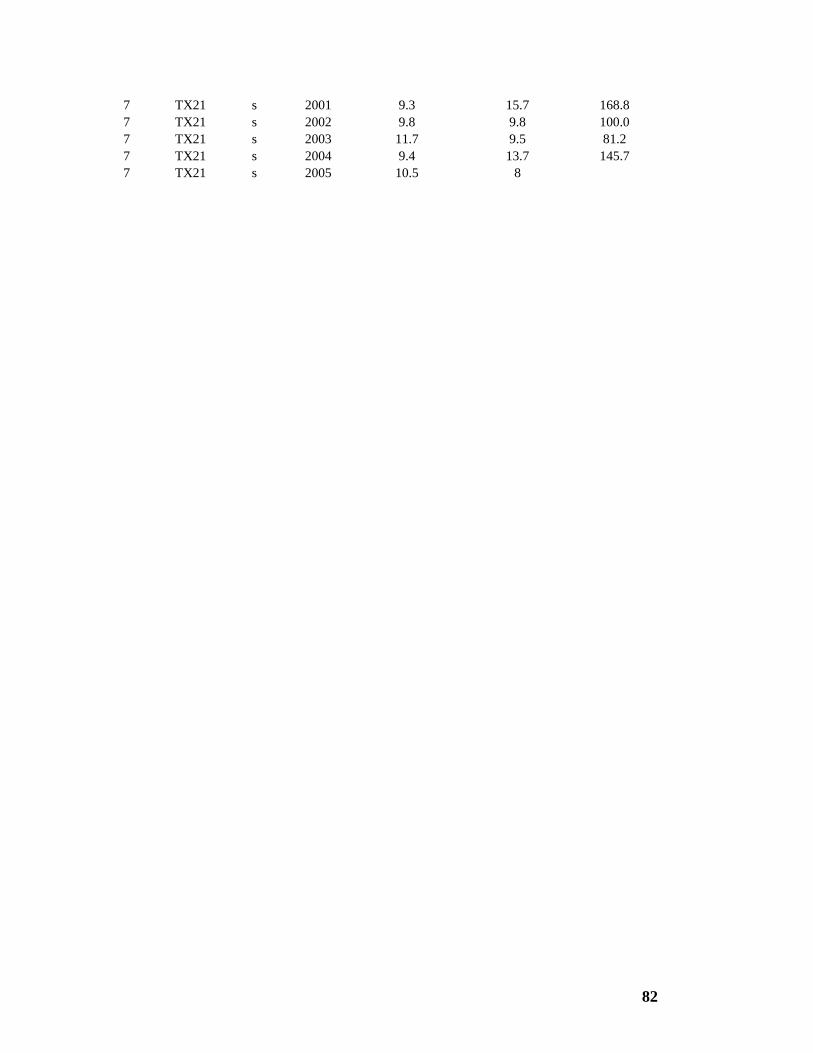
82

7 TX21 s 2001 9.3 15.7 168.8 7 TX21 s 2002 9.8 9.8 100.0 7 TX21 s 2003 11.7 9.5 81.2 7 TX21 s 2004 9.4 13.7 145.7 7 TX21 s 2005 10.5 8

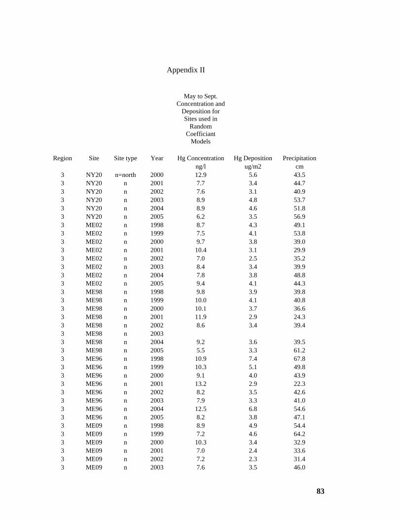
83

Appendix II

May to Sept. Concentration and

Deposition for Sites used in

Random Coefficiant

Models

Region Site Site type Year Hg Concentration Hg Deposition Precipitation ng/l ug/m2 cm

3 NY20 n=north 2000 12.9 5.6 43.5 3 NY20 n 2001 7.7 3.4 44.7 3 NY20 n 2002 7.6 3.1 40.9 3 NY20 n 2003 8.9 4.8 53.7 3 NY20 n 2004 8.9 4.6 51.8 3 NY20 n 2005 6.2 3.5 56.9 3 ME02 n 1998 8.7 4.3 49.1 3 ME02 n 1999 7.5 4.1 53.8 3 ME02 n 2000 9.7 3.8 39.0 3 ME02 n 2001 10.4 3.1 29.9 3 ME02 n 2002 7.0 2.5 35.2 3 ME02 n 2003 8.4 3.4 39.9 3 ME02 n 2004 7.8 3.8 48.8 3 ME02 n 2005 9.4 4.1 44.3 3 ME98 n 1998 9.8 3.9 39.8 3 ME98 n 1999 10.0 4.1 40.8 3 ME98 n 2000 10.1 3.7 36.6 3 ME98 n 2001 11.9 2.9 24.3 3 ME98 n 2002 8.6 3.4 39.4 3 ME98 n 2003 3 ME98 n 2004 9.2 3.6 39.5 3 ME98 n 2005 5.5 3.3 61.2 3 ME96 n 1998 10.9 7.4 67.8 3 ME96 n 1999 10.3 5.1 49.8 3 ME96 n 2000 9.1 4.0 43.9 3 ME96 n 2001 13.2 2.9 22.3 3 ME96 n 2002 8.2 3.5 42.6 3 ME96 n 2003 7.9 3.3 41.0 3 ME96 n 2004 12.5 6.8 54.6 3 ME96 n 2005 8.2 3.8 47.1 3 ME09 n 1998 8.9 4.9 54.4 3 ME09 n 1999 7.2 4.6 64.2 3 ME09 n 2000 10.3 3.4 32.9 3 ME09 n 2001 7.0 2.4 33.6 3 ME09 n 2002 7.2 2.3 31.4 3 ME09 n 2003 7.6 3.5 46.0

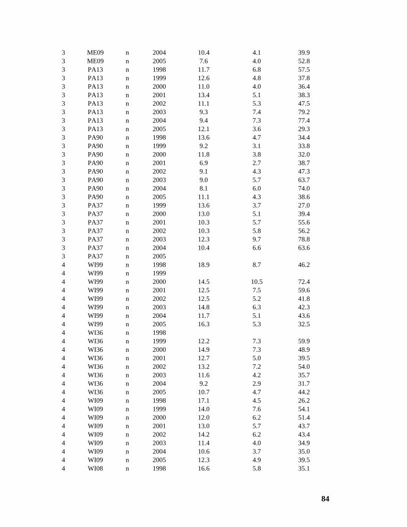
84

3 ME09 n 2004 10.4 4.1 39.9 3 ME09 n 2005 7.6 4.0 52.8 3 PA13 n 1998 11.7 6.8 57.5 3 PA13 n 1999 12.6 4.8 37.8 3 PA13 n 2000 11.0 4.0 36.4 3 PA13 n 2001 13.4 5.1 38.3 3 PA13 n 2002 11.1 5.3 47.5 3 PA13 n 2003 9.3 7.4 79.2 3 PA13 n 2004 9.4 7.3 77.4 3 PA13 n 2005 12.1 3.6 29.3 3 PA90 n 1998 13.6 4.7 34.4 3 PA90 n 1999 9.2 3.1 33.8 3 PA90 n 2000 11.8 3.8 32.0 3 PA90 n 2001 6.9 2.7 38.7 3 PA90 n 2002 9.1 4.3 47.3 3 PA90 n 2003 9.0 5.7 63.7 3 PA90 n 2004 8.1 6.0 74.0 3 PA90 n 2005 11.1 4.3 38.6 3 PA37 n 1999 13.6 3.7 27.0 3 PA37 n 2000 13.0 5.1 39.4 3 PA37 n 2001 10.3 5.7 55.6 3 PA37 n 2002 10.3 5.8 56.2 3 PA37 n 2003 12.3 9.7 78.8 3 PA37 n 2004 10.4 6.6 63.6 3 PA37 n 2005 4 WI99 n 1998 18.9 8.7 46.2 4 WI99 n 1999 4 WI99 n 2000 14.5 10.5 72.4 4 WI99 n 2001 12.5 7.5 59.6 4 WI99 n 2002 12.5 5.2 41.8 4 WI99 n 2003 14.8 6.3 42.3 4 WI99 n 2004 11.7 5.1 43.6 4 WI99 n 2005 16.3 5.3 32.5 4 WI36 n 1998 4 WI36 n 1999 12.2 7.3 59.9 4 WI36 n 2000 14.9 7.3 48.9 4 WI36 n 2001 12.7 5.0 39.5 4 WI36 n 2002 13.2 7.2 54.0 4 WI36 n 2003 11.6 4.2 35.7 4 WI36 n 2004 9.2 2.9 31.7 4 WI36 n 2005 10.7 4.7 44.2 4 WI09 n 1998 17.1 4.5 26.2 4 WI09 n 1999 14.0 7.6 54.1 4 WI09 n 2000 12.0 6.2 51.4 4 WI09 n 2001 13.0 5.7 43.7 4 WI09 n 2002 14.2 6.2 43.4 4 WI09 n 2003 11.4 4.0 34.9 4 WI09 n 2004 10.6 3.7 35.0 4 WI09 n 2005 12.3 4.9 39.5 4 WI08 n 1998 16.6 5.8 35.1

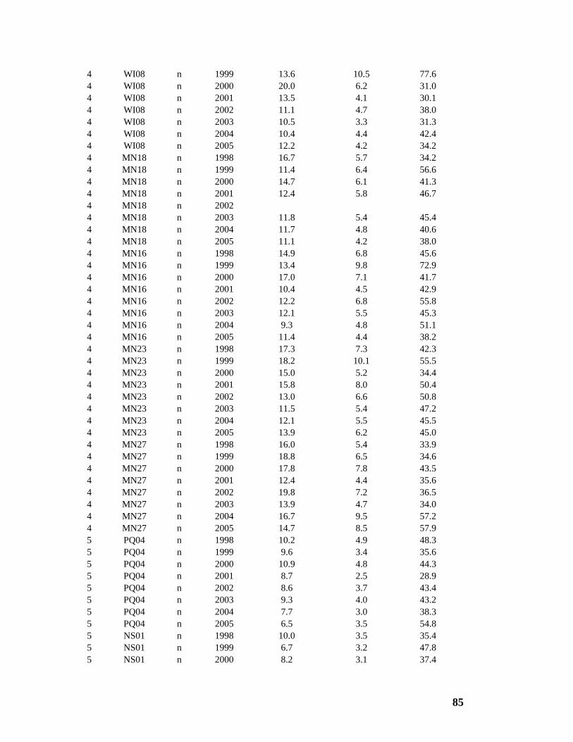
85

4 WI08 n 1999 13.6 10.5 77.6 4 WI08 n 2000 20.0 6.2 31.0 4 WI08 n 2001 13.5 4.1 30.1 4 WI08 n 2002 11.1 4.7 38.0 4 WI08 n 2003 10.5 3.3 31.3 4 WI08 n 2004 10.4 4.4 42.4 4 WI08 n 2005 12.2 4.2 34.2 4 MN18 n 1998 16.7 5.7 34.2 4 MN18 n 1999 11.4 6.4 56.6 4 MN18 n 2000 14.7 6.1 41.3 4 MN18 n 2001 12.4 5.8 46.7 4 MN18 n 2002 4 MN18 n 2003 11.8 5.4 45.4 4 MN18 n 2004 11.7 4.8 40.6 4 MN18 n 2005 11.1 4.2 38.0 4 MN16 n 1998 14.9 6.8 45.6 4 MN16 n 1999 13.4 9.8 72.9 4 MN16 n 2000 17.0 7.1 41.7 4 MN16 n 2001 10.4 4.5 42.9 4 MN16 n 2002 12.2 6.8 55.8 4 MN16 n 2003 12.1 5.5 45.3 4 MN16 n 2004 9.3 4.8 51.1 4 MN16 n 2005 11.4 4.4 38.2 4 MN23 n 1998 17.3 7.3 42.3 4 MN23 n 1999 18.2 10.1 55.5 4 MN23 n 2000 15.0 5.2 34.4 4 MN23 n 2001 15.8 8.0 50.4 4 MN23 n 2002 13.0 6.6 50.8 4 MN23 n 2003 11.5 5.4 47.2 4 MN23 n 2004 12.1 5.5 45.5 4 MN23 n 2005 13.9 6.2 45.0 4 MN27 n 1998 16.0 5.4 33.9 4 MN27 n 1999 18.8 6.5 34.6 4 MN27 n 2000 17.8 7.8 43.5 4 MN27 n 2001 12.4 4.4 35.6 4 MN27 n 2002 19.8 7.2 36.5 4 MN27 n 2003 13.9 4.7 34.0 4 MN27 n 2004 16.7 9.5 57.2 4 MN27 n 2005 14.7 8.5 57.9 5 PQ04 n 1998 10.2 4.9 48.3 5 PQ04 n 1999 9.6 3.4 35.6 5 PQ04 n 2000 10.9 4.8 44.3 5 PQ04 n 2001 8.7 2.5 28.9 5 PQ04 n 2002 8.6 3.7 43.4 5 PQ04 n 2003 9.3 4.0 43.2 5 PQ04 n 2004 7.7 3.0 38.3 5 PQ04 n 2005 6.5 3.5 54.8 5 NS01 n 1998 10.0 3.5 35.4 5 NS01 n 1999 6.7 3.2 47.8 5 NS01 n 2000 8.2 3.1 37.4

86

5 NS01 n 2001 8.1 2.7 33.8 5 NS01 n 2002 5 NS01 n 2003 6.3 3.3 53.4 5 NS01 n 2004 7.8 2.8 35.8 5 NS01 n 2005 6.1 2.9 47.3 6 IL11 n 1999 6 IL11 n 2000 12.7 6.5 51.3 6 IL11 n 2001 15.0 5.8 38.5 6 IL11 n 2002 6 IL11 n 2003 12.9 6.9 53.2 6 IL11 n 2004 13.5 6.2 45.8 6 IL11 n 2005 12.0 4.9 40.6 1 FL34 s=south 1998 13.0 19.1 146.9 1 FL34 s 1999 11.9 9.8 983.3 1 FL34 s 2000 20.5 11.6 1158.9 1 FL34 s 2001 13.3 14.3 1427.0 1 FL34 s 2002 14.0 6.4 642.9 1 FL34 s 2003 18.8 14.6 1455.8 1 FL34 s 2004 12.5 7.9 793.9 1 FL34 s 2005 12.8 9.8 76.9 1 FL05 s 1999 11.9 10.5 88.1 1 FL05 s 2000 14.0 11.4 81.3 1 FL05 s 2001 13.4 9.5 71.1 1 FL05 s 2002 15.5 11.1 71.2 1 FL05 s 2003 20.6 13.1 63.6 1 FL05 s 2004 16.0 14.2 89.0 1 FL04 s 1998 16.6 14.5 87.3 1 FL04 s 1999 14.2 14.4 101.6 1 FL04 s 2000 20.1 14.7 73.1 1 FL04 s 2001 14.4 16.8 116.8 1 FL04 s 2002 15.8 15.8 99.7 1 FL04 s 2003 17.7 22.5 127.0 1 FL04 s 2004 16.2 12.8 79.2 1 FL11 s 1998 14.5 14.5 100.0 1 FL11 s 1999 13.9 14.7 105.1 1 FL11 s 2000 15.8 15.9 100.4 1 FL11 s 2001 17.0 15.3 90.0 1 FL11 s 2002 13.5 15.0 111.2 1 FL11 s 2003 18.1 21.0 115.8 1 FL11 s 2004 16.9 13.8 81.3 1 FL11 s 2005 10.8 15.4 143.2 2 NC42 s 1998 10.0 6.0 59.4 2 NC42 s 1999 6.8 5.1 74.5 2 NC42 s 2000 9.5 7.7 81.0 2 NC42 s 2001 9.2 4.3 47.4 2 NC42 s 2002 9.8 4.3 44.5 2 NC42 s 2003 8.3 5.8 69.7 2 NC42 s 2004 10.2 7.9 77.6 2 NC42 s 2005 8.1 5.5 68.5 2 NC08 s 1998 15.1 10.2 67.3

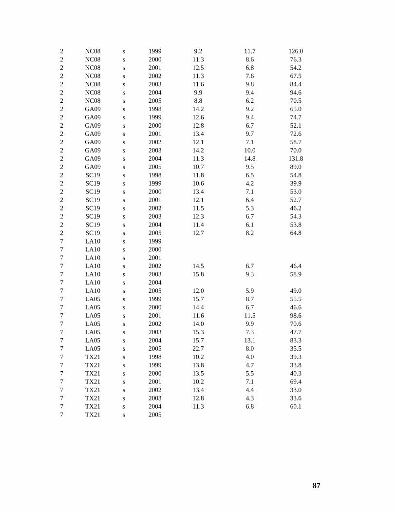
87

2 NC08 s 1999 9.2 11.7 126.0 2 NC08 s 2000 11.3 8.6 76.3 2 NC08 s 2001 12.5 6.8 54.2 2 NC08 s 2002 11.3 7.6 67.5 2 NC08 s 2003 11.6 9.8 84.4 2 NC08 s 2004 9.9 9.4 94.6 2 NC08 s 2005 8.8 6.2 70.5 2 GA09 s 1998 14.2 9.2 65.0 2 GA09 s 1999 12.6 9.4 74.7 2 GA09 s 2000 12.8 6.7 52.1 2 GA09 s 2001 13.4 9.7 72.6 2 GA09 s 2002 12.1 7.1 58.7 2 GA09 s 2003 14.2 10.0 70.0 2 GA09 s 2004 11.3 14.8 131.8 2 GA09 s 2005 10.7 9.5 89.0 2 SC19 s 1998 11.8 6.5 54.8 2 SC19 s 1999 10.6 4.2 39.9 2 SC19 s 2000 13.4 7.1 53.0 2 SC19 s 2001 12.1 6.4 52.7 2 SC19 s 2002 11.5 5.3 46.2 2 SC19 s 2003 12.3 6.7 54.3 2 SC19 s 2004 11.4 6.1 53.8 2 SC19 s 2005 12.7 8.2 64.8 7 LA10 s 1999 7 LA10 s 2000 7 LA10 s 2001 7 LA10 s 2002 14.5 6.7 46.4 7 LA10 s 2003 15.8 9.3 58.9 7 LA10 s 2004 7 LA10 s 2005 12.0 5.9 49.0 7 LA05 s 1999 15.7 8.7 55.5 7 LA05 s 2000 14.4 6.7 46.6 7 LA05 s 2001 11.6 11.5 98.6 7 LA05 s 2002 14.0 9.9 70.6 7 LA05 s 2003 15.3 7.3 47.7 7 LA05 s 2004 15.7 13.1 83.3 7 LA05 s 2005 22.7 8.0 35.5 7 TX21 s 1998 10.2 4.0 39.3 7 TX21 s 1999 13.8 4.7 33.8 7 TX21 s 2000 13.5 5.5 40.3 7 TX21 s 2001 10.2 7.1 69.4 7 TX21 s 2002 13.4 4.4 33.0 7 TX21 s 2003 12.8 4.3 33.6 7 TX21 s 2004 11.3 6.8 60.1 7 TX21 s 2005