final report non-co2 climate forcers

1

Abatement opportunities for non-CO2 climate forcers Black carbon, methane, nitrous oxide and f-gas emissions reductions to complement CO2 reductions and enable national environmental and social objectives

Briefing paper, May 2011

2

Major Findings

While there is still much uncertainty around the emissions and abatement opportunities for black carbon, methane, nitrous oxide and f-gases, enough is now known to inform action.

These non-CO2 climate forcers collectively cause at least one quarter of global warming and accelerate the rate of temperature change.

In addition, black carbon and methane contribute significantly to air pollution, which causes millions of premature deaths and even higher rates of disease.

Emissions from the four non-CO2 climate forcers can be reduced by over 20 percent by 2030 using available methods: fugitive emissions capture, efficient agricultural practices, combustion optimization, diesel particulate controls, and alternative cooling technologies.

Reducing non-CO2 emissions is essential to limit global warming during this century, slow the rate of temperature increase, and reduce the risk of adverse climate feedbacks.

On top of the positive climate effects, 80 percent of the measures also improve public health and half come at a net savings to society.

While a large share of the measures is relatively straightforward to implement, capturing the remainder will be challenging, as millions of people would need to take action, some of whom are the world’s poorest.

In developed countries, the principal abatement opportunities lie in waste management, air conditioning and refrigeration, and diesel engines.

Opportunity areas for developing countries are diesel engines, natural gas production, waste management, and traditional combustion technologies.

None of the measures in this report can substitute for the immediate and massive carbon dioxide reductions needed for long-term climate stabilization. Non-CO2 mitigation measures are complementary to CO2 controls.

3

Table of Contents

Preface 4

Executive Summary 6

Study approach 16

Global perspective on non-CO2 climate forcers 20

Non-CO2 climate forcer perspectives

Black Carbon 43

Methane 56

Nitrous oxide 62

F-Gases 66

References 74

Appendix A: Key contacts and contributors 82

Appendix B: Glossary 84

Appendix C: Abatement potential in 2020 87

Appendix D: Black and organic carbon in tonnes 92

Appendix E: Areas of further research 93

Appendix F: Alternative metrics considerations 93

Appendix G: List of major assumptions 94

4

Preface Greenhouse gas (GHG) emissions have risen significantly over the past 15 years, from 36 gigatonnes of carbon dioxide equivalent (GtCO2e) in 1990 to over 45 GtCO2e in 2005. The net effect of black carbon1 accounts for an additional 6 GtCO2e of global warming emissions in 2005. Black carbon is a climate forcing aerosol that is not part of the Kyoto protocol, and thus has not yet received as much attention as the GHGs. Without collective attempts to curb emissions, GHGs and net black carbon combined are likely to grow to about 75 GtCO2e by 2030. However, many scientific estimates suggest that emissions would instead need to fall dramatically by that point in order to maintain a chance of keeping global warming to within 2 degrees Celsius—the level above which dangerous climate changes occur.2

To date, most attention has been focused on carbon dioxide (CO2), as it accounts for the largest share of human-induced global warming emissions. Also, most scientists agree that CO2 emissions will determine the climate outcome a century from today and beyond, since it is the most abundant long-lived gas. But nearer term effects are also important. Methane, nitrous oxide, the fluorinated gases (f-gases), and black carbon are expected to account for over 25 percent of the total global warming impact in 2030. These four main non-CO2 emissions3 exert a powerful influence on the climate. Their radiative forcing is between 20 and 20,000 times greater on a unit basis than CO2. They accelerate the rate of temperature change, which in turn affects the ability of ecosystems to adapt. Black carbon also reduces the reflectivity of snow and ice, causing those surfaces to melt faster than they otherwise would, threatening the Arctic and the world's glacier systems. Methane is a precursor to ozone, which damages plant tissues thereby reducing their ability to sequester CO2.

Furthermore, black carbon and methane are contributors to air pollution, adding to unhealthy levels of fine particulate matter and ground level ozone throughout the world.

Taking action to reduce these non-CO2 emissions therefore delivers a triple benefit. First, it complements national and international efforts to reduce CO2, increasing the chances of climate stabilization in the medium to longer term4. Second, reducing emissions of methane and black carbon increases the resilience of the planet’s ecosystem, preserving natural

1 The warming effect of black carbon, net of the cooling effect of co-emitted organic carbon. 2 den Elzen and Meinshausen (2006); den Elzen et al. (2007); den Elzen and van Vuuren (2007); Meinshausen (2006); and

Ramanathan and Xu (2010). 3 Not included here are several other non-CO2 climate forcers, such as sulfur dioxide (which has a cooling effect) and other warming

emissions, such as volatile organic compounds and carbon monoxide, that are smaller in size. 4 “Failing to reduce carbonaceous aerosol emissions requires a greater reduction in CO2 emissions to meet the same Radiative Forcing equivalent or temperature target.” Kopp and Mauzerall (2010).

5

carbon sinks, glaciers, and Arctic ice. Third, controlling methane and black carbon emissions reduces air pollution, improving public health.5

Actions that improve public health produce an economic benefit to society through greater productivity. In addition, some of the black carbon abatement measures can more directly work to alleviate poverty. For example, improving access to clean fuels for residential cooking and heating would substantially reduce the labor required to collect dirtier biomass fuels. The time savings could then be applied to productive economic activity that increases personal wealth.

This report is intended to provide a fact base for policymakers, companies, and NGOs on these four important non-CO2 climate forcers. Specifically, it seeks to:

■ Describe their impact, highlighting the role of black carbon

■ Quantify expected emissions development in the absence of any major policy changes

■ Assess and quantify abatement opportunities in terms of mass, cost, and investment requirements

■ Assess the main additional benefits of reducing emissions, particularly the impact on public health

The results of this analysis, especially the relative magnitude of the emissions, may be new to many readers. Previous reports on greenhouse gas abatement have included some analysis of methane, nitrous oxide, and f-gas emissions,6 but not at the level of detail in this report. Black carbon was not included at all. For all of the climate forcers we have used the most updated emissions inventories and projections available. That said, research is ongoing and refined data is expected from several institutions in the near future.

The principal metric used in this report is 100-year Global Warming Potential (GWP 100) carbon dioxide equivalent (CO2e). This is the standard metric used by the Intergovernmental Panel on Climate Change (IPCC) to compare different climate forcers with one another. However, readers should understand that short-lived climate forcers are distinctly different from CO2 in time and space. Methane and black carbon have much more immediate climate impacts than carbon dioxide, but then disappear from the atmosphere unless replenished with new emissions. For black carbon, the majority of those impacts may be further restricted to discrete regional areas. Conversely, CO2 and other long-lived gases (including nitrous oxide and some f-gases) are globally mixed into relatively uniform concentrations and remain for in the atmosphere for centuries.

5 Details on health impacts and benefits can be found in the "Study Approach" and respective "Climate Forcer Perspectives" chapters. 6 Based on McKinsey & Company, 2009.

6

By using 100-year CO2e GWP values, it is not our intent to imply that all climate forcers are equal or interchangeable. There are several good scientific reasons to handle short and long term climate forcers differently.7 Rather, our goal is to convey that non-CO2 pollutants are a significant part of the climate change problem and to put that contribution into perspective. There are a number of remaining uncertainties concerning both the level of emissions from non-CO2 climate forcers and the abatement potential. Nevertheless, the analysis at hand provides a strong indication that large-scale efforts should be made to reduce non-CO2 emissions, in order to tackle climate change and air pollution.

We have produced this report in cooperation with a global network of leading academics, government bodies, think tanks, NGOs, and companies in order to incorporate the most up-to-date and detailed understanding of climate science and emission abatement. McKinsey & Company provided analytical support for this report based on its global and national greenhouse gas abatement studies. We would like to thank all of these individuals and organizations for their contributions. The full list of contributors is included in Appendix A.

7 “We need to separate the policy frameworks and interventions for attending to short-lived versus long-lived climate forcing agents… The physical properties, sources and policy levers of short-lived forcing agents – black soot, aerosols, methane and tropospheric ozone – are quite different from those of long-lived forcing agents – carbon dioxide, halocarbons, nitrous oxide.” Molina et al., 2009. “One potential alternative to the single greenhouse gas basket approach is to have several baskets with trading only within each particular one. While still imperfect, if the baskets contain gases of comparable lifetimes, the confounding tradeoffs of short- vs. long-lived gases will be reduced in importance.” Daniel et al., 2009.

7

Executive Summary This report is intended to provide a fact base for policymakers, companies, and NGOs to better understand methane, nitrous oxide, f-gases, and black carbon. It identifies the climate, health, and environmental impacts of these non-CO2 climate forcers and assesses abatement opportunities.

While there is still much uncertainty around the emissions and abatement opportunities for black carbon, methane, nitrous oxide, and f-gases, enough is now known to inform action. The state of knowledge for these four climate forcers is less advanced than for carbon dioxide for two reasons. First, emissions estimates are less precise for non-CO2 climate forcers since some source categories are more difficult to measure and there have been fewer analyses conducted. For example, some methane comes from leaks that are difficult to identify and from biological sources that are subject to varying conditions. Second, there is some uncertainty about the magnitude of the effect that each climate forcer has on temperature increase. The current state of science regarding radiative forcing values for black carbon includes an uncertainty range of almost ±50 percent and there is considerable uncertainty about aerosol and cloud interactions.

There is a policy dimension as well, since the international climate community has not come to consensus yet on the best way to compare short-lived and long-lived climate forcers. The 100-year and 20-year CO2 equivalent values discussed in this report are just a rough approximation of what is actually happening in the atmosphere. In reality, long lived forcers can persist for thousands of years and certain short lived forcers leave the atmosphere within days. The geographical location of climate impacts also varies depending on whether the pollutant is uniformly mixed in the global atmosphere or regionally constrained.

Fortunately, there is a rapidly growing body of research that has helped to narrow these uncertainties. Methane, nitrous oxide, and f-gases are included in the Kyoto Protocol and therefore have been a part of national submissions to the UNFCCC, and of several other inventory and future projection analyses. Black carbon, while not included in these submissions, is being actively studied by several leading researchers8 with a number of publications upcoming in 2011. Additionally, there is an international scientific debate on climate metrics underway which is expected to be reflected in the next major Assessment Report of the IPCC, currently scheduled for 2014.

Some have argued that there are too many uncertainties surrounding those non-CO2 climate forcers for policymakers to take any decisive action. However, the conclusion of this

8 See, for example, Bond 2007; IIASA’s GAINS model; and Fuglestvedt 2009.

8

research is that the uncertainties involved do not detract from the main findings. Whatever climate metric is applied, non-CO2 climate forcers clearly cause a substantial portion of global warming. In addition, black carbon and methane emissions increase air pollution and consequential disease and premature mortality. A range of abatement measures exists that can be quantified to capture both climate and associated public health benefits.

These non-CO2 climate forcers collectively cause at least one quarter of global warming9 and accelerate the rate of temperature change CO2 is the most prevalent of the greenhouse gases (GHGs) and among the longest lasting in the atmosphere. As such, it is the single biggest cause of long-term climate change and the focus of most discussions and efforts to reduce emissions. Yet there are a number of other, significant non-CO2 “climate forcers” that have received less focus. These are methane, nitrous oxide, fluorinated gases (f-gases), and black carbon.

These four climate forcers are emitted from a variety of sources (Exhibit 1). Methane and nitrous oxide arise from biological processes in agriculture and waste decomposition, and from certain industrial processes. F-gases are used as coolants in refrigeration and air conditioning and are emitted to a lesser extent from industrial processes. Black carbon, an aerosol and component of soot, results from incomplete combustion—that is, when a carbonaceous fuel fails to get fully converted into CO2. Major sources of human-induced black carbon are diesel engines, traditional brick kilns and coke ovens, and domestic cookstoves.

These non-CO2 climate forcers will account for over 25 percent of the global warming impact from emissions in 2030 from a 100-year perspective. They have an even greater impact over shorter time scales. Hence, reducing these emissions in parallel to CO2

abatement would therefore play an important role in stabilizing the climate by slowing the rate of temperature change.10 (These concepts are discussed in more detail in the “Study Approach - Climate Metrics” chapter.)

9 Using 100-year GWP carbon dioxide equivalent metric. 10 See, for example, Molina et al., 2009; Kopp and Mauzerall, 2010; and Ramanathan and Xu, 2010.

9

EXHIBIT 1

Non-CO2 climate forcers – emission sources

▪ GHG, emitted from industries and anaerobic digestion▪ Precursor to tropospheric

ozone which causes disease and inhibits growth of vegetation

Description and impact

Methane(CH4)

SOURCE: Non-CO2 Climate Forcers Report (2010); IPCC Second Assessment Report (SAR) (1995); IPCC Fourth Assessment Report (AR4) (2007); Rypdalet al. (2009)

Nitrous oxide(N2O)

Fluorinated gases (F-gases)

Black carbon

12 years

Lifetime

72

20-year

21

100-year

114 years 289310

Varies byf-gas(HFC-134a: 14 years)

Main sources

▪ Livestock▪ Petroleum and

gas production▪ Rice farming▪ Waste

decomposition

▪ GHG, primarily formed through chemical processes in agricultural soils

▪ Fertilizers▪ Manure

management▪ Acid production

▪ GHG, used as coolants (refrigeration, air-conditioning), accelerants and insulators

▪ Refrigeration ▪ Air conditioning▪ Electric power

transmission▪ HCFC-22

production

▪ Carbonaceous aerosol, emitted as product of incomplete combustion▪ Co-emitted with other

particulates that combined have strong negative health effects ▪ Increases the rate of Arctic and

glacial melting

▪ Diesel engines▪ Brick kilns and

coke ovens▪ Biomass and

coal cookstoves

1-2 weeks3,230917

Varies byf-gas(HFC-134a: 1,300)


NOTE: 100-year GWP expressed in SAR values; 20-year GWP expressed in AR4 values

Global Warming Potential (GWP)

In addition, black carbon and methane contribute significantly to air pollution, which causes millions of premature deaths and even higher incidence of disease Emissions from non-CO2 climate forcers affect not only climate change, but also public health. Although significant strides have been made toward a cleaner, healthier atmosphere, globally millions of people are still exposed to dangerous levels of air pollution – especially in the developing world. Every year, more than 3 million people11 worldwide die from respiratory problems, cardiovascular problems, and lung cancer caused by indoor and outdoor air pollution. Premature mortality, illness, and lost productivity reduce quality of life and undercut national GDP growth in several developing nations.

Black carbon and methane contribute to this public health burden by adding to fine particulate matter12 and tropospheric ozone concentrations,13 respectively, both of which are

11 Approximately 1.2 million deaths attributable to urban outdoor air pollution and 2.0 million deaths attributable to indoor smoke

from solid fuels (WHO, 2009). 12 “Fine particulate matter” refers to particles that are 2.5 microns in diameter or smaller. Black carbon particles are below 1 micron

in diameter, in the 1-100 nanometer range. (A nanometer is about 1/50,000 the diameter of a human hair.)

10

important components of air pollution. Fine particulate matter is the most damaging air pollutant worldwide, with the highest morbidity and premature mortality impacts of any air pollutant. Tropospheric ozone exposures also lead to increased disease and, in some cases, death, but the incidence rates are significantly lower.

Emissions from the four non-CO2 climate forcers can be reduced by over 20 percent by 2030 using available methods: fugitive emissions capture, efficient agricultural practices, combustion optimization, diesel particulate controls, and alternative cooling technologies Emissions from the non-CO2 climate forcers are forecast to grow by nearly 30 percent between 2005 and 2030 in the business-as-usual case (from 15.8 GtCO2e to 20.1 GtCO2e GWP100). There is potential to reduce emissions from non-CO2 climate forcers in 2030 by over 20 percent, or 4.5 GtCO2e from the business-as-usual (BAU) levels, through technical abatement measures.14Capturing this total abatement potential would eliminate growth in non-CO2 emissions. Behavioral changes would provide additional abatement potential, with the biggest opportunity being up to 1.8 GtCO2e from reduced meat and dairy consumption. There are five major opportunities for abatement of non-CO2 forcers (Exhibit 2):

■ Capturing fugitive emissions from gas handling, coal mining, and waste management ■ Improved agricultural practices to curb methane and nitrous oxide emissions ■ Improved combustion technologies to reduce black carbon emissions ■ Improving cooling technologies to reduce emissions of f-gases ■ Reduced transport particulate emissions, particularly from diesel engines

More than 50 percent of the abatement potential comes at a net profit to society, meaning that subsequent economic benefits outweigh the initial investment and incremental operating costs. For example, the cost of capturing methane gas generated from landfill sites can be recouped through the value of electricity generated with the methane. Another 30 percent of the abatement potential can be captured at a cost of $20/tCO2e or less. Nearly all of the remaining abatement, though more expensive, would deliver important health and other non-climate-related environmental benefits.

13 Pew Center, 2009; and Smith, K., 2009. Tropospheric ozone is also referred to as "ground level ozone." Methane is one of several precursors to ground level ozone and contributes mostly to background ozone levels (as opposed to peak concentrations) because of its relatively low reactivity.

14 Uncertainty analysis shows that at minimum the abatement potential is 3.5 GtCO2e, but it is likely to be over 5 GtCO2e.

11

EXHIBIT 2

SOURCE: Non-CO2 Climate Forcers Report (2010)

Key opportunities

Improved combustion technologies

0.5 15.61.0

Abatement Case2030

Improved cooling technologies

0.7

Capturing fugitive emissions

20.1

BAUgrowth

15.8 4.3

BAUEmissions 2005

1.8

Improved agricultural practices

0.6

Reduced transportation particulateemissions

BAUEmissions 2030

-22%

▪ Water and nutrient management in rice cultivation▪ Anti-methanogen

vaccines and feed supplements for livestock

▪ Improved cookstoves and LPG cookstoves▪ Replacing

traditional kilns with vertical shaft and tunnel kilns

▪ Emission controls for on-road and off-road vehicles, particularly heavy-duty diesel trucks

▪ Landfill gas capture ▪ Oxidation of coal

mine ventilationair and mine degasification▪ Electrostatic

precipitators for coke ovens

▪ Low GWP coolants for motor vehicle air conditioning▪ Lower leakage in

retail food refrigeration using secondary loops or distributed systems

Abatement divided into categories for actionGtCO2e (GWP 100) per year

~40% ~20% ~20% ~10% ~10%

X% Share of total abatement potential

Reducing non-CO2 emissions is essential to limit global warming during this century, slow the rate of temperature increase, and reduce the risk of adverse climate feedbacks There are three angles from which to assess the need for urgency to reduce the non-CO2 climate forcers in parallel to carbon dioxide: limiting the total amount of global warming; reducing the rate of temperature increase; and reducing the risk of adverse climate feedbacks on both a global and regional scale.

Ultimately, long-term temperature increases and temperature stabilization levels after mitigation will be determined by the level and pathway of carbon dioxide emissions, the most prevalent GHG. Still, abating non-CO2 climate forcers in parallel to CO2 is essential to achieving temperature stabilization at all. Even assuming no growth in non-CO2 emissions after 2030, there would be about 20 GtCO2e of emissions without abatement. This amount represents nearly all of, if not more than, the total emissions per year that could be perpetually emitted without further increasing the temperature, i.e., to enable temperature stabilization. No abatement of the non-CO2 forcers would essentially mean that CO2 emissions would need to be cut close to zero in order to achieve stabilization.

In the short-term, non-CO2 abatement has an even greater impact on slowing the rate of temperature increase, due to the high short-term warming effect of those climate forcers.

12

The rate of change in local climate has implications for the ability of those ecosystems to adapt– the faster the change, the lower the ability to adapt, the higher the risk of irreversible changes. Berntsen et al. demonstrated that drastically reducing non-CO2 climate forcers in the short term prolongs the time needed to reach maximum temperatures by several decades – slowing the rate of change, thus improving the ability of humans and ecosystems to adapt.15 Van Vuuren et al. confirm this finding and conclude that multi-gas abatement scenarios are also the most cost-effective way to contain warming.16

Moreover, reducing black carbon would help alleviate non-temperature related climate changes, such as the melting of glaciers and arctic ice. Abating methane, which as a precursor of tropospheric ozone damages vegetation, would improve the ability of plants to sequester carbon.17 These are both areas where abatement would substantially reduce adverse climate feedbacks.

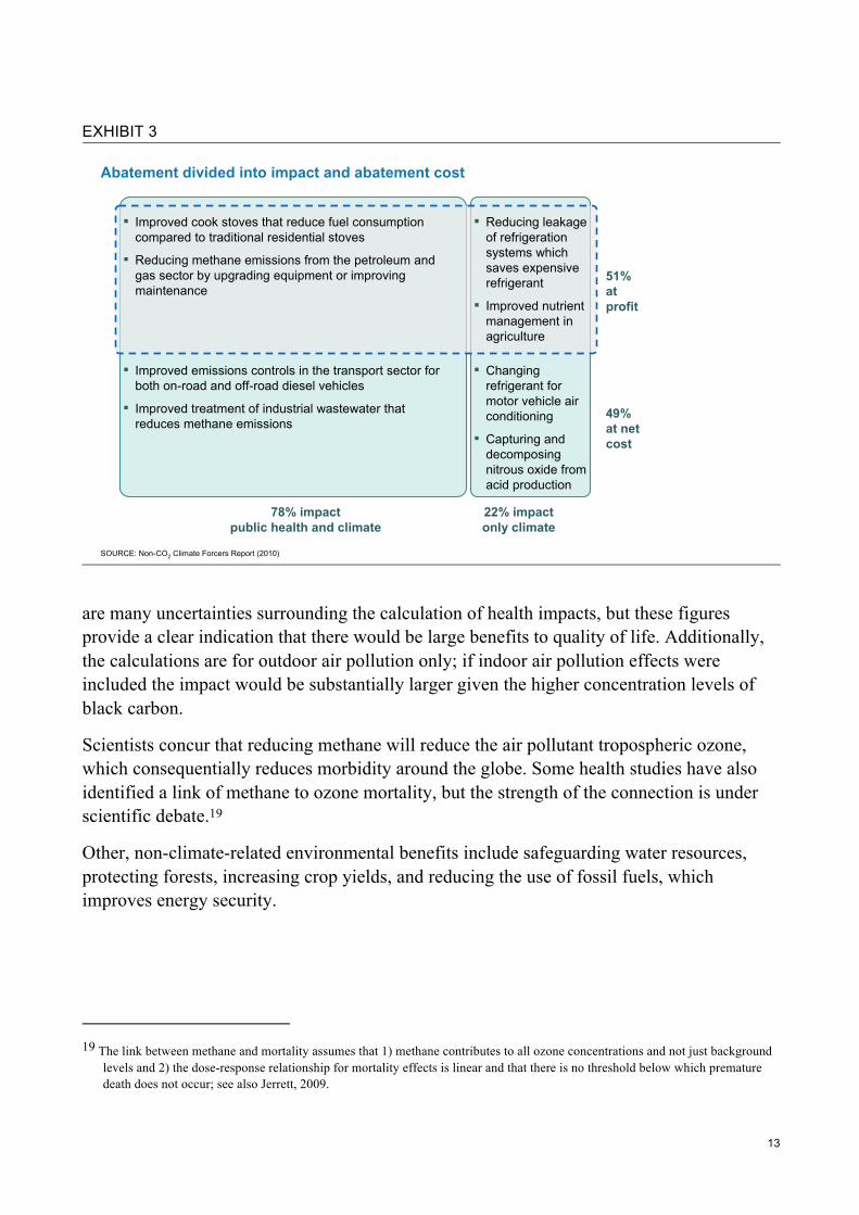
On top of the positive climate effects, 80 percent of the measures also improve public health and half come at a net savings to society Reducing methane and black carbon emissions will deliver near-term health benefits. Nearly 80 percent of the abatement measures result in air pollution reduction, thereby improving public health (Exhibit 3). The remaining 20 percent of abatement can be divided into those measures that result in a net societal profit (such as refrigerant leak prevention) and those that are pure global climate change mitigation measures (such as industrial nitrous oxide controls). Overall, half of the measures come at societal profit, independent of whether the motivation to pursue them is improved public health or purely climate change.

The health and quality of life benefits from reducing air pollution are substantial. Using IIASA's health models, life expectancies in China and India were found to be reduced by an average of 3 years per person due to air pollution of particulate matter under business-as-usual conditions.18 This is an average over the entire population, but only a subset of the population actually dies of air pollution influenced causes. For the individuals affected, years of life lost are substantially higher. Using the same models, it was found that if the full abatement potential of black carbon were captured in China and India, life expectancies in 2030 in these countries could be increased by an average of 2-4 months per person. There

15 Berntsen et al., CICERO, 2010. Temperature increase target set at 1.5°C warming. In the case of the same abatement for all

climate forcers, maximum temperature is reached after 50 years (1.5% p.a. rate of temperature increase); whereas in the case of drastic non-CO2 reduction it takes 80 years (1.0% p.a.).

16 Van Vuuren et al., 2006. Including non-CO2 gases is crucial in the formulation of a cost-effective abatement response, and can reduce costs by 30-40 percent compared to a CO2 only reduction strategy for the same radiative forcing target.

17 Royal Society, 2008. 18 Amann et al, 2008a, and additional GAINS model runs for this study.

13

EXHIBIT 3

Abatement divided into impact and abatement cost


51%at profit

49%at netcost

78% impactpublic health and climate

22% impactonly climate

▪ Improved cook stoves that reduce fuel consumption compared to traditional residential stoves

▪ Reducing methane emissions from the petroleum and gas sector by upgrading equipment or improving maintenance

▪ Improved emissions controls in the transport sector for both on-road and off-road diesel vehicles

▪ Improved treatment of industrial wastewater that reduces methane emissions

▪ Reducing leakage of refrigeration systems which saves expensive refrigerant

▪ Improved nutrient management in agriculture

▪ Changing refrigerant for motor vehicle air conditioning

▪ Capturing and decomposing nitrous oxide from acid production

Updated 100706

are many uncertainties surrounding the calculation of health impacts, but these figures provide a clear indication that there would be large benefits to quality of life. Additionally, the calculations are for outdoor air pollution only; if indoor air pollution effects were included the impact would be substantially larger given the higher concentration levels of black carbon.

Scientists concur that reducing methane will reduce the air pollutant tropospheric ozone, which consequentially reduces morbidity around the globe. Some health studies have also identified a link of methane to ozone mortality, but the strength of the connection is under scientific debate.19

Other, non-climate-related environmental benefits include safeguarding water resources, protecting forests, increasing crop yields, and reducing the use of fossil fuels, which improves energy security.

19 The link between methane and mortality assumes that 1) methane contributes to all ozone concentrations and not just background

levels and 2) the dose-response relationship for mortality effects is linear and that there is no threshold below which premature death does not occur; see also Jerrett, 2009.

14

While a large share of the measures is relatively straightforward to implement, capturing the remainder will be challenging, as millions of people would need to take action, some of whom are the world’s poorest Reducing emissions of non-CO2 forcers is comparatively straightforward on some dimensions. In many cases, there is little infrastructure “lock in” since emissions sources such as refrigerators and diesel engines are replaced every 10 to 15 years. In cases of capital intensive assets, such as coal mines or landfills, there are “end of pipe” technologies available that do not require stock replacement. Moreover, the technologies are largely already available today, well understood, and relatively simple.

However, half of the abatement potential for non-CO2 climate forcers comes at a net cost to society. And even those measures that come at a net profit, such as more efficient brick kilns, may prove difficult to finance as the initial investments are needed from some of the world’s poorest. Individual families, rural farmers, and small businesses will have significant difficulty in gathering the necessary capital for new appliances, diesel retrofits, or alternative fertilizers. The very poor will have no ability to switch cookstoves without direct financial assistance. Governments wanting to pursue these abatement measures will have to devise both regulatory and fiscal policies to address these challenges.

Additionally, many of the sources of non-CO2 emissions are relatively small and diffuse, such as agricultural emissions. The majority of the abatement opportunity is in the developing world where many countries are not as well equipped with institutions or resources to reach and change the conduct of thousands – or sometimes millions – of individuals. These countries will need to develop regulatory expertise to set standards, and enforce as well as monitor progress towards goals, such as those set for industrial mandates. For other measures, such as in agriculture, the expertise and capacity to educate people on emissions abatement measures will need to be built up.

In developed countries, the principal abatement opportunities lie in waste management, air conditioning and refrigeration, and diesel engines The developed world has taken significant strides to reduce air pollution, and climate change legislation has either been enacted, as in the European Union, or is under consideration. However, there are a number of further steps that can be taken to reduce emissions from the non-CO2 forcers that will complement efforts to reduce CO2 emissions.

The three areas with the largest abatement potential are: the reduction of emissions from landfills, either through methane capture or composting; the reduction of f-gas emissions by using new coolants in motor vehicle air conditioning and new systems for retail food refrigeration; and, in the near term, retrofitting of existing vehicles with diesel engine particulate controls.

15

Opportunity areas for developing countries are diesel engines, natural gas production, waste management and traditional combustion technologies In the developing world, different social, economic, environmental, and health objectives vie for resources. Nonetheless, significant efforts have been made to reduce air pollution and to increase energy efficiency in order to improve public health and limit climate warming. Further potential exists to reduce the non-CO2 forcers, which will complement these efforts.

The developing world will account for over 80 percent of non-CO2 emissions in 2030. Thus, in line with CO2, it is the developing world that has the largest abatement potential, and it is there that most investments will be required to capture that potential.

Four emissions sources could each provide around 15 percent of the total abatement potential: diesel engines, natural gas production, waste management, and traditional combustion technologies. Diesel engine particulate controls for new on-road and off-road vehicles would reduce health-damaging black carbon emissions. Methane emissions that are vented during natural gas production and from solid waste landfills can be captured and utilized. Improving traditional combustion technologies—such as cook stoves and brick kilns—would both increase energy efficiency and reduce black carbon. At about 10 percent each of the total abatement opportunity, changed rice growing and livestock practices can reduce emissions, though these are challenging to implement.


Carbon dioxide accounts for more than half of global warming. Its atmospheric concentration has risen 35 percent since 1750 and is now at about 390 ppmv, the highest level in 800,000 years. Annual CO2 emissions must be reduced more than 80 percent to stabilize carbon dioxide concentrations in the atmosphere. If global CO2 emissions peak in the next decade and fall to 50-85 percent of 2000 levels by 2050, global mean temperature increases could be limited to 2.0-2.4°C above pre-industrial levels.20 The need for CO2 reductions is urgent. Even a few years' delay in the peak can mean the world is committed to a significantly higher temperature rise than would otherwise be the case - for every ten years the peak is postponed, another half degree of temperature increase becomes unavoidable.21

Non-CO2 mitigation measures will not eliminate the need for massive CO2 reductions but can ease the pathway to long-term climate stabilization. Non-CO2 measures will slow the

20 Climate Stabilization Targets: Emissions, Concentrations, and Impacts over Decades to Millennia, 2011, National Research Council. 21 Dr. Vicky Pope, Hadley Centre, Director of Climate Change, 2008.

16

rate of temperature change over the next several decades. The near- and mid-term benefits of non-CO2 abatement will also reduce the risk of triggering irreversible tipping points in the earth’s climate system, as well as capturing public health benefits. Combining CO2 and non-CO2 strategies, therefore, offers the greatest chance of achieving the limitation to 2 degrees Celsius of warming adopted in the Copenhagen Accord.

17

Study approach There are three parts to the analysis of non-CO2 climate forcer abatement. The first is the choice of climate metrics to quantify the global warming impact of the four non-CO2 forcers. The second is to determine the business-as-usual (BAU) emissions baseline, as well as the abatement potential and cost, forming the abatement cost curve. The third examines the non-climate related benefits of abatement, with a focus on public health.

Climate metrics

This section covers the metrics chosen to quantify climate “forcing” – the impact that GHGs and aerosols have on the energy balance of the earth. The potency of a climate forcer is characterized by its radiative forcing and its global warming potential. The concepts of radiative forcing (RF) and global warming potential (GWP) were introduced in the late 1980s. Now enshrined in the Kyoto Protocol, RF and GWP are the prevailing climate metrics in the international climate community.

Radiative Forcing is the rate of energy change from a pulse of emissions, per square meter, at the top of the atmosphere. RF may be positive (warming) or negative (cooling). RF values come from satellite data, climate models, and direct observations in laboratory or field experiments. RF can be direct (from the emissions themselves) or indirect (from the interaction of those emissions with other physical factors, such as clouds or rain).

Global Warming Potential is defined as cumulative radiative forcing, over a specified time period, from one unit of a given climate forcer’s emissions, relative to the same mass of carbon dioxide which is by definition valued at one (1.0). Since the mass of the two pollutants being compared is the same, GWP values can then used to calculate metric tonnes of CO2 equivalent (tCO2e). Carbon dioxide is the basis of comparison for all GWP values because it is the primary cause of anthropogenic climate change. GWP values come from multiple data sets and analyses, the most comprehensive of which are set forth in the IPCC AR4 from 2007.

Different climate forcers endure in the atmosphere for different periods of time. For example, CO2 persists almost infinitely while black carbon falls to the surface within days. Climate forcers with shorter lifetimes trap more heat initially but diminish in potency over time. Long-lived climate forcers, by contrast, are dominant over extended periods of time. To capture these differences, GWP values are calculated over a specific time interval to reflect the total relative warming effect of the forcers over that interval.

18

EXHIBIT 4

Metrics options

SOURCE:Non-CO2 Climate Forcers Report (2010); IPCC SAR, IPCC AR4; Fuglestvedt, 2009

Global Warming Potential –20 Year (GWP20)

InstantaneousRadiative Forcing (RF)

Global Warming Potential –100 Year (GWP100)

Communication units▪ W/m2 ▪ CO2e (GWP20) ▪ CO2e (GWP100)

Description▪ Additional energy captured

in the Earth-atmosphere system by a climate forcer, as a reference to the base concentration in the atmosphere

▪ Time integral of radiative forcing over 20 yrs for a “pulse of emissions” (e.g. 1 kg)

▪ Expressed in terms of equivalent radiative forcing over the period that would result from a “pulse” of CO2

▪ Time integral of radiative forcing over 100 yrs for a “pulse of emissions” (e.g. 1 kg)

▪ Expressed in terms of equivalent radiative forcing over the period that would result from a “pulse” of CO2

Advantages▪ Pure physical discussion▪ Captures climate effect of

each climate forcer

▪ Accounts for fact that climate change occurs over long time scales and forcers have different atmospheric lifetimes

▪ Comparability across climate forcers

▪ Most commonly used metric, familiar to policy makers

▪ Accounts for fact that climate change occurs over long time scales and gases have different atmospheric lifetimes

▪ Comparability across climate forcers

Drawbacks▪ RF value is an instantaneous

value upon emission, does not include lifetime effect

▪ Assumes all radiative forcing acts equally on climate, but in models shown to depend on location, season, etc.

▪ Not familiar to policy makers

▪ Timescale-dependent, with value placed on near-term effects

▪ Assumes all radiative forcing acts equally on climate, but actually varies on location, season, etc.

▪ Partly familiar to policy makers though not highly used in the literature

▪ Timescale-dependent, with value placed on long-term effects

▪ Assumes all radiative forcing acts equally on climate, but in models shown to depend on location, season, etc.

Mass of climate forcer

▪ Metric tonne

▪ Mass of climate forcer emitted over a period of time

▪ Pure physical discussion▪ Warming potentials could

be applied later as needed

▪ Would not give a clear indication of relative importance of different forcers to allow comparison

Methane Example▪ 1.82 x 10-13 W/m2/kg ▪ 72 (AR4) ▪ 21 (SAR)▪ 1 metric tonne (t)

Updated 100630 –latest in report

In this study, we use 100-year GWP to describe the long-term effects of climate forcing and to calculate CO2 equivalents. The values for 100-year GWP are taken from the IPCC’s 2004 Second Assessment Report to conform this report to previous cost curves for GHGs and to US EPA's baseline values. This is the most common climate metric in the world and is used widely in policy discussions and by international climate organizations like the UNFCCC. It is also the basis for international emission trading regimes, meaning that policy concerns can arise whenever the metric is employed in new ways (see below). Climate scientists view 100-year GWP as the best available compromise for comparing short and long lived species, though it has severe limitations at both temporal extremes (very short and very long time spans).

By using 100-year GWP values, it is not our intent to imply that all climate forcers are equal or interchangeable. For example, we are not advocating that black carbon be added to international emission trading schemes simply because it can be expressed in CO2e units. Trading rules and other international climate agreements are beyond the scope of this report. Rather, we used 100-year GWP values to convey the relative weight of non-CO2 measures to each other and to compare their aggregate impact to prior work on GHG abatement cost curves. We believe that tonnage-based calculations are a useful orientation to mitigation options even if they do not perfectly capture how the climate responds to various interventions.

19

To describe the impact that the non-CO2 forcers have on the rate of temperature change, a shorter-term perspective, we applied 20-year GWP values in this study. Methane, with a lifetime of 12 years, has a GWP of 21 over the 100-year interval but a much stronger GWP of 72 over the 20-year interval. For 20-year GWP calculations, the values from the IPCC’s 2007 Fourth Assessment Report are used, reflecting the latest scientific assessment. Global average GWP values for black and organic carbon are derived from Rypdal et al. (2009) and fall in the mid-range of recent estimates.22 (Exhibit 4.)

There is no “correct” or “perfect” GWP value. Focusing on near term effects generates higher values for short-lived forcers. Conversely, long-lived climate forcers show the highest warming potential over a century or more (Exhibit 5). Both metrics are only rough approximations of what is actually happening in the atmosphere. Moreover, neither 100-year nor 20-year GWP values convey the full range of climate effects or regional differences. Detailed atmospheric modelling with high scale geographical resolution is needed for the latter. The IPCC has recognized that new metrics are needed and commissioned a special committee on this topic. A more detailed discussion of these issues is provided in Appendix F.

22 See e.g., Bond, 2007; Boucher and Reddy, 2008; and Rypdal et al., 2009.

20

EXHIBIT 5

Source: IPCC AR4 WG3, Figure 2.22, 2007.

21

Business as usual emissions and abatement cost curve

The analysis starts with an understanding of the business-as-usual emissions trajectory from 2005 to 2030. The inventory of emissions in 2005 is used as the base year, as this is the last year in which reliable data can be gathered from across sectors and climate forcers. The 2005 inventory is then extrapolated into the future using several methods, including basing future growth off historical growth patterns or in projecting activity data, such as with the number of vehicles in the transportation sector, and then estimating future emissions based on emissions factors, i.e., the amount of climate forcer emitted per unit of activity. For methane, nitrous oxide, and f-gases, the analyses rely mainly on assessments by the US Environmental Protection Agency’s (US EPA) 2006 Global Anthropogenic Emissions Report, as well as other complementing sources. The effect of CDM projects on BAU emissions is accounted for to the extent that the US EPA included it in their analyses. For black carbon, emissions factors are largely drawn from Bond (2007) and the GAINS model from the International Institute for Applied Systems Analysis (IIASA, 2010), and were compared against estimates by Tsinghua University in Beijing. Energy-use data have been derived from the International Energy Agency (IEA), GAINS, and other sources. The BAU assumptions are described in more detail in Appendix F.

The methodology used to calculate the abatement potential and cost is based on that used in McKinsey's Pathways to a Low-carbon Economy (2009), which is similar to that used by other researchers in the field. The combined axes of an abatement cost curve depict the available technical measures, their relative impact (volume reduction potential), and cost in a specific year. Potential and cost are incremental to the BAU case (Exhibit 6).

The width of each bar on the cost curve represents the technical potential (not a forecast) to reduce emissions by that measure, assuming that implementation starts in 2010. This technical potential assumes concerted action to capture the opportunity. The height of each bar represents the average cost of avoiding one metric tonne of carbon dioxide equivalent (tCO2e). Abatement costs are defined as the incremental cost of a low-emission technology compared with the BAU case measured as USD/tCO2e of abated emissions. Abatement costs include annualized incremental capital expenditure and changes in operating expenditure. The cost therefore represents the “project cost” of installing and operating the low-emission technology, and excludes transaction costs such as capacity building, education, and enforcement monitoring. Transaction costs will depend on the policies chosen to incentivize implementation.

22

EXHIBIT 6

Abatement cost curve methodology

SOURCE: McKinsey

Abatement cost USD/tCO2e

Abatement potentialtCO2e per year

Width quantifies emission reduction potential relative to BAU

Height quantifies incremental cost relative to BAU (incremental annualized capital costs plus change in net operating costs)

Abatement cost[Full cost of CO2e efficient alternative] [Full cost of reference solution]–

[CO2e emissions from alternative][CO2e emissions from reference solution] –=

Updated 100630 –latest in text

The cost curve takes a societal perspective instead of that of a specific decision-maker, such as a company or a consumer, illustrating the costs required of the society. The societal perspective uses a real long-term government bond rate of 4 percent for repayments, based on historical global averages for long-term bond rates. Furthermore, subsidies, taxes, and CO2 prices are excluded. From an investor/decision-maker perspective, there could be higher costs, such as an increased cost of capital or tax implications.

The societal perspective enables the usage of the abatement cost curve as a fact base for global and country discussions about what levers exist to reduce emissions, how to compare reduction opportunities and costs between countries and sectors, and how to discuss what incentives (e.g., subsidies, taxes, and CO2 pricing) to put in place. While we realize that the choice of which emission reduction measures to implement involves many non-economic considerations, this societal project economics perspective can be a useful starting point for discussions on how to reduce emissions and prioritize abatement action.

It has been necessary to make many assumptions in order to estimate the impact and cost of the abatement opportunities. We believe all figures are reasonable estimates given the information available, but they inevitably contain uncertainty. Each step of the analysis contains a degree of uncertainty—the emissions inventory, the emissions growth trajectory, the scientific assessment of the climate impact of each climate forcer, the abatement potential, and the abatement cost. The largest areas of uncertainty for the purposes of this

23

report are the emissions inventory, GWP values, and the abatement implementation shares. Given these uncertainties, a Monte Carlo analysis was used to describe the range of abatement potentials that might be expected. (For further discussion of the uncertainties, see the Global Perspective chapter of this report.)

Health benefits It is very difficult to calculate the health benefits of non-CO2 interventions for three reasons. The first obstacle is data availability. Measurements of existing air pollution exposures and mortality rates are limited, and some countries have no ambient particulate measurements at all (a necessary prerequisite to evaluating black carbon changes). The second obstacle is methodological. Large-scale air quality models are substantially less reliable than higher resolution urban air shed models, adding a higher degree of uncertainty. The third and final problem is imprecision about the effect of each technological intervention. For all of these reasons, the health analyses below should be viewed as indicative rather than determinative.

To analyze the impact of the abatement of black carbon on health, IIASA performed calculations with their scientific air pollution model, described in their GAINS model documentations.23 For methane, this analysis is based on scientific studies by West et al.24 and Fiore et al.25 More information about the air pollution and health effects of black carbon, methane, and tropospheric ozone can be found, for example, in documents from the Pew Center26 and Smith.27

Black Carbon: IIASA's GAINS model determines the effect of particulate matter PM2.5 emissions, which are directly associated with black carbon, on a decrease in statistical life expectancy. When assessing the benefit of black carbon abatement, the difference between two cases is calculated: the business-as-usual case and the abatement case. This will show the improvement of statistical average life expectancy due to abatement.

In detail, IIASA describes the approach as follows: "For Asia (i.e., China, India, Pakistan), the GAINS analysis uses annual mean PM2.5 concentrations of primary particulate matter (black carbon, organic

carbon, other organic matter, mineral dust, etc.) and secondary inorganic aerosols emitted from anthropogenic sources as calculated with the GAINS model (based on

23 Amann et al., 2008a; Amann et al., 2008b. 24 West et al., 2006. 25 Fiore et al., 2008. 26 Pew Center, 2009. 27 Smith, K., 2009.

24

TM5 calculations), distinguishing in each grid cell urban background and rural concentrations. The health impact calculation does not quantify impacts from emissions from natural sources and of secondary organic aerosols

population maps with a 1*1 degree resolution distinguishing urban and rural population in each grid cell

population projections by cohort up to 2030 from IIASA’s World Population programme by country

epidemiological evidence on premature mortality as reported by Pope et al., 2002 for the United States and the relative risk numbers given in this paper

life tables that quantify current mortality rates for different cohorts for China, India, Pakistan, as well as the life table of Japan, from the UN population database

The current GAINS calculation assumes a linear exposure-response curves up to the concentrations calculated for future years (i.e., up to 200 µg/m3) based on the findings of the PAPA study (2004)."

IIASA also takes into account uncertainties around applicable rate of health risk and baseline mortality rates. The results represent the mean of the uncertainty analysis.

For this report, the black carbon analysis was undertaken for China and India only and separately, as these are the countries where the abatement potential for particulate matter is greatest. It should be noted that the model only calculates the effect on health of lowering outdoor air pollution levels. Lowering indoor air pollution levels from cookstoves would have greater impact given the very direct exposure of people, particularly women and children, to pollutants from that source category.

Methane: Health is affected via tropospheric ozone, to which methane is a precursor. Tropospheric ozone is also referred to as ground level ozone. Ozone is a secondary pollutant that is formed through complex photochemical reactions involving nitrogen oxides and volatile organic compounds in the presence of ultraviolet sunlight. Tropospheric ozone concentrations have doubled worldwide since preindustrial times.

Studies identified a significant association between long-term ozone exposure and cardiovascular, cardiopulmonary, and respiratory health issues. Ozone has also been associated with morbidity, including asthma exacerbation and hospital admissions for respiratory causes. Some studies (West, Fiore, Jerrett) also indicate a link between ozone exposure and premature mortality, and suggest a linear dose-response relationship. However, the strength of the mortality finding at low ozone concentrations is scientifically debated and there is not yet consensus. 28

28 Smith, K., 2009.

25

Methane abatement first reduces emissions of methane, then, with a time lag, atmospheric concentrations of methane, which subsequently lowers the levels of tropospheric ozone, improving health. We relied in our health benefits calculation on two main studies: West et al.29 calculated the impact on premature deaths from a constant 20 percent reduction in methane emissions starting in 2010 and sustained into 2030. A constant reduction of 65 Mt of methane per year would result in approximately 30,000 reduced premature all-cause mortalities in 2030.

In detail, West et al. state: "We first estimate the global decrease in surface O3 concentration due to CH4 mitigation, using the MOZART-2 global three-dimensional tropospheric chemistry transport model. This spatial distribution of O3 is then overlaid on projections of population, and avoided premature mortalities are estimated by using daily O3-mortality relationships from epidemiologic studies from Bell and others."

The study from Fiore et al.30 demonstrated how scenarios like this can be used to calculate the health impact for different abatement pathways. Based on these studies, premature, all-cause mortality in 2030 is derived from the abatement potential identified in this study.31

Those calculations are founded on two key assumptions for the link between methane and mortality: 1) methane contributes to all ozone concentrations and not just background levels and 2) the dose-response relationship for mortality effects is linear and there is no threshold below which premature death does not occur.

Knowledge about the connections between methane and health effects is still nascent, e.g., in models to analyze global levels of tropospheric ozone or the contribution of methane to background vs. peak level ozone. Jerrett et al.32 released a study in which the researchers "were unable to detect a significant effect of exposure to ozone on the risk of death from cardiovascular causes when particulates were taken into account, but... did demonstrate a significant effect of exposure to ozone on the risk of death from respiratory causes." Scientific work is ongoing to better understand these linkages.

29 West et al., 2006. 30 Fiore et al., 2008. 31 The 2030 number gives a conservative picture of the health benefits. In 2030, only 51 percent of the full positive health effect of

abatement is reached due to time lag between cause and action. In 2050, 90 percent of the full effect could be observed based on modelling, if abatement is kept at a constant level.

32 Jerrett et al., 2009.

26

Global perspective on non-CO2 climate forcers

Black carbon, methane, nitrous oxide, and f-gases collectively cause at least one quarter of global warming and accelerate the rate of temperature change. In addition, black carbon and methane contribute significantly to air pollution, which causes millions of premature deaths and even higher incidence of disease

Emissions sources for non-CO2 climate forcers CO2 is the most common of the greenhouse gases (GHGs) and one of the longest lived in the atmosphere. It is therefore the largest contributor to long-term temperature increase, both in terms of the impact of historical emissions since the industrial revolution and of that of today’s emissions.33 Most studies that assess abatement opportunities have therefore focused on CO2, highlighting actions to transition to an economy that burns dramatically less fossil fuel and avoids deforestation.

There are a number of other “climate forcers,”34 however, that contribute towards climate change. Those with the greatest emissions volume are methane, nitrous oxide, the fluorinated gases (f-gases), and black carbon. These are the focus of this report due to their relatively strong warming impact and the quantity of emissions.

Black carbon, methane, nitrous oxide, and f-gases are emitted from a variety of sources (Exhibit 7). Methane and nitrous oxide arise from biological processes in agriculture and waste decomposition, and from certain industrial processes. F-gases are used as coolants in refrigeration and air conditioning and are emitted to a lesser extent from industrial processes. Black carbon, an aerosol, results from incomplete combustion—that is, when a carbonaceous fuel fails to be fully converted into CO2. The main sources of human-induced black carbon emissions are diesel engines, industrial and domestic kilns and stoves, agricultural burning, and planned forest fires. In this report, the global warming potential (GWP) of black carbon is net of the cooling effect of organic carbon, which is co-emitted in the combustion process.35 (See sidebar, “Climate effects of black carbon.”)

33 IPCC Fourth Assessment Report, 2007. 34 We use the term “climate forcers” as a summary term for the greenhouse gases and aerosols that have an impact on the energy

balance of the Earth. See the GWP Sidebar. 35 Combustion processes also emit other pollutants such as CO and SO2. Their climate effects have not been included in the net

effect of black carbon as shown in this report.

27

EXHIBIT 7

Non-CO2 climate forcers – emission sources

▪ GHG, emitted from industries and anaerobic digestion▪ Precursor to tropospheric

ozone which causes disease and inhibits growth of vegetation

Description and impact

Methane(CH4)

SOURCE: Non-CO2 Climate Forcers Report (2010); IPCC Second Assessment Report (SAR) (1995); IPCC Fourth Assessment Report (AR4) (2007); Rypdalet al. (2009)

Nitrous oxide(N2O)

Fluorinated gases (F-gases)

Black carbon

12 years

Lifetime

72

20-year

21

100-year

114 years 289310

Varies byf-gas(HFC-134a: 14 years)

Main sources

▪ Livestock▪ Petroleum and

gas production▪ Rice farming▪ Waste

decomposition

▪ GHG, primarily formed through chemical processes in agricultural soils

▪ Fertilizers▪ Manure

management▪ Acid production

▪ GHG, used as coolants (refrigeration, air-conditioning), accelerants and insulators

▪ Refrigeration ▪ Air conditioning▪ Electric power

transmission▪ HCFC-22

production

▪ Carbonaceous aerosol, emitted as product of incomplete combustion▪ Co-emitted with other

particulates that combined have strong negative health effects ▪ Increases the rate of Arctic and

glacial melting

▪ Diesel engines▪ Brick kilns and

coke ovens▪ Biomass and

coal cookstoves

1-2 weeks3,230917



NOTE: 100-year GWP expressed in SAR values; 20-year GWP expressed in AR4 values

Global Warming Potential (GWP)

While all four of the non-CO2 climate forcers increase global warming, methane and black carbon also have additional climate effects. Black carbon influences the hydrological cycle and snow and ice coverage. Methane, as a precursor to tropospheric ozone, impairs crop growth. These climate-related effects are explained in more detail in later chapters.

Methane and black carbon also damage health.36 Although significant strides have been made towards reducing air pollution around the globe, millions of people are still exposed to dangerous levels—especially in the developing world. Every year, more than 3 million people37 die from respiratory problems, cardiovascular problems, and lung cancer caused by indoor and outdoor air pollution. Illness and premature death are the result, which undercuts productivity and GDP growth in several developing nations.

Business-as-usual growth In 2005, emissions from the four non-CO2 climate forcers were 15.8 GtCO2e, accounting for 30 percent of total global warming emissions. This is in addition to the 35.6 Gt of

36 See the chapter "Study Approach" for details. 37 Approximately 1.2 million deaths annually are attributable to urban outdoor air pollution and 2.0 million deaths attributable to

indoor smoke from solid fuels (WHO, 2009).

28

carbon dioxide emissions in 2005. As previous reports38 did not include net black carbon, the total emissions in 2005 are larger than previously communicated, totalling 51.4 GtCO2e. By 2030, emissions of the four non-CO2 climate forcers are expected to grow to 20.1 GtCO2e, and their share of total emissions will fall slightly to 27 percent. This is due to the faster annual growth of CO2 emissions (1.7 percent per year) compared with the non-CO2 forcers (1.0 percent per year) (Exhibit 8).

Because most non-CO2 climate forcers are short-lived compared with CO2, and because they have a higher GWP, they have a greater short-term impact on the climate and the rate of temperature change. Using a 20-year GWP, the non-CO2 forcers account for 50 percent of global warming (Exhibit 9). This higher short-term effect of the non-CO2 forcers provides a ready opportunity to slow the rate of temperature increase.

EXHIBIT 8

Business as usual emissions of the four non-CO2 forcers and CO2

1 Net of co-emitted Organic Carbon

6

8

9

5

4

3

5

5

6

Carbon Dioxide (CO2)

MethaneNitrous OxideF-gases

Net Black Carbon1

2030

75

55

2

2020

66

48

1

2005

51

36

1

Long-term perspective (100 years)

GtCO2e (GWP 100) per year

Covered in previous ClimateWorks reports

Covered in this report

27% contribution

SOURCE: Non-CO2 Climate Forcers Report (2010); Pathways to a low-carbon economy (2009); IEA WEO2009; IPCC SAR (1995); IPCC AR4(2007); US EPA Global Anthropogenic Emissions Report (2006)

38 McKinsey & Company, 2009.

29

EXHIBIT 9

Comparison of near-term and long-term global warming impact

27%

50%

73%

50%

Non-CO2climateforcers

CO2

Near-term (20yr GWP)Long-term (100yr GWP)

SOURCE: Non-CO2 Climate Forcers Report (2010); Pathways to a low-carbon economy (2009); IEA WEO2009; IPCC SAR (1995); IPCC AR4(2007); US EPA Global Anthropogenic Emissions Report (2006)

Percent of total GtCO2e – 2030

Contribution to global warming

In 2030, methane will account for the largest share of non-CO2 emissions (43 percent), followed by net black carbon (26 percent),39 nitrous oxide (23 percent), and the f-gases (8 percent). Increases in methane and nitrous oxide over the time period are strongly tied to population growth, which drives more waste creation and more intensive farming methods. The f-gases are the fastest growing of all the climate forcers, growing at an annual rate of around 5 percent. A switch to f-gases to replace the ozone-depleting substances (ODS) that were previously used as coolants and accelerants, as well as an increase in demand for refrigeration and air conditioning in the developing world, explains this rapid growth. Black carbon emissions, on the other hand, will fall slowly. Many sources of black carbon, such as inefficient wood cook stoves and the brick kilns and coke ovens used in industry, are associated with lower levels of economic development. As wealth grows, black carbon emissions from these sources should fall, although the gains are somewhat offset by overall growth in fuel usage (Exhibit 10).

Agriculture accounts for the largest proportion of non-CO2 climate forcers (approximately 50 percent). Emissions from the sector show steady annual growth of 1 percent between 2005 and 2030. Emissions from petroleum and gas, part of the industry sector, and the residential and commercial sectors will grow slightly faster as a result of higher GDP growth and higher consumption. Emissions from the transportation sector and other sub-sectors of

39 Net black carbon is the warming impact of black carbon net of the cooling effect of co-emitted organic carbon.

30

the industry sector will grow more slowly thanks to increased energy efficiency, stricter regulations, and industry initiatives to reduce f-gas emissions.

It should be noted that figures both for current and future emissions are difficult to measure accurately. This is explained in detail later in this chapter.

EXHIBIT 10

Business as usual emissions of non-CO2 climate forcers

1 Net of co-emitted organic carbon2 For regional consistency, Mexico is in Latin America and not Other OECDSOURCE: Non-CO2 Climate Forcers Report (2010)

5.6

5.1

1.6

Methane

Nitrousoxide

F-gases

Netblackcarbon1

2030

20.1

8.7

4.7

2005

15.8

6.5

3.3

0.5

1.2

4.7

1.5

-0.3

1.0Total

3.1

4.0

1.9

1.9

Agriculture/forestry

Waste

Residential/commercial

Industry

Transport

2030

20.1

9.8

1.8

2.6

2005

15.8

7.7

1.4

1.8

Total

0.9

1.0

1.6

1.1

0.1

1.0

By climate forcer

Othernon-OECD

Africa

LatinAmerica2

India

China

OtherOECD2

EU 27US

2030

20.1

4.6

3.7

3.1

1.6

3.3

1.21.2

1.5

2005

15.9

3.6

2.7

2.2

1.1

2.7

1.01.3

1.3

Total

0.9

1.0

1.0

-0.50.4

1.0

1.5

1.4

1.3

Annual growth, 2005–2030Percent

By sector By region


Emissions from the four non-CO2 climate forcers can be reduced by over 20 percent by 2030 using available methods: fugitive emissions capture, efficient agricultural practices, combustion optimization, diesel particulate controls, and alternative cooling technologies

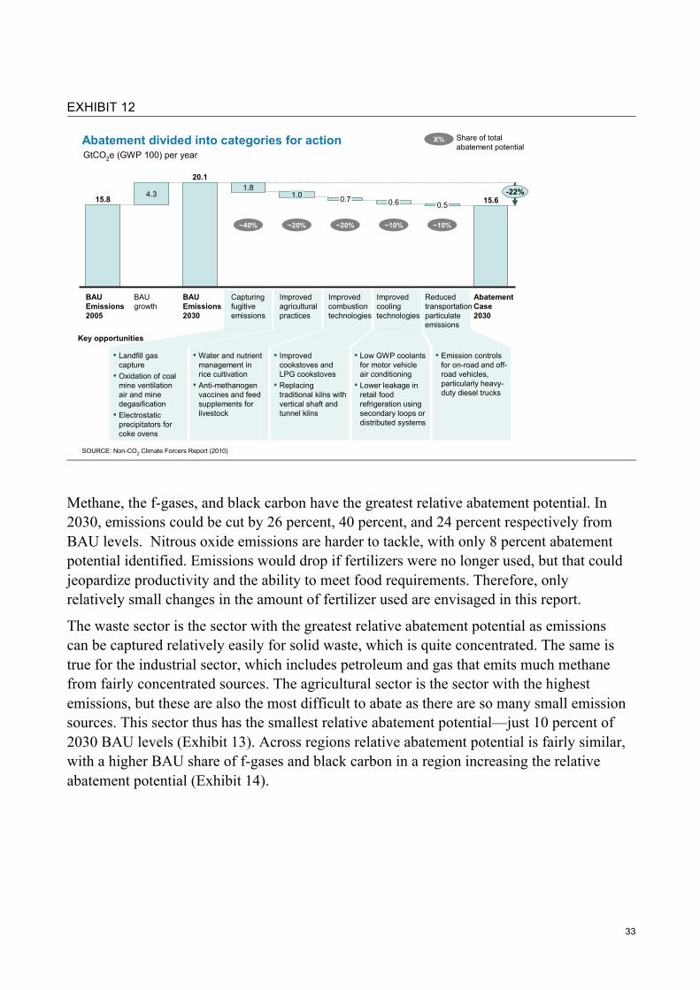
Abatement potential Using the technical abatement measures identified in this report, there is potential to reduce emissions from the non-CO2 climate forcers by over 20 percent, or 4.5 GtCO2e, from BAU levels in 2030. Implementing the measures would also cut CO2 emissions by 0.8 Gt, bringing the total to 5.3 GtCO2e and effectively eliminating growth in non-CO2 emissions by 2030. Behavioral change, which was not analyzed in detail in this report, would provide additional abatement potential, the biggest opportunity being up to 1.8 GtCO2e from reduced consumption of meat and dairy products.

The 50 abatement measures with the largest potential were assessed and quantified for this report. There are remaining measures, including those that would reduce PFC emissions

31

(an f-gas), which were not quantified in the costs curves. These are estimated to have a total global additional reduction potential of about 0.5 GtCO2e.

There are five major groups of opportunities for abatement of non-CO2 forcers (Exhibits 11 and 12):

Capturing fugitive emissions (1.8 GtCO2e of abatement potential in 2030): Climate forcers emitted from industrial and waste processes can be captured and often re-used. For example, methane can be used to generate electricity, while f-gases can be recycled or destroyed. Examples of the way emissions can be captured include the installation of gas capturing systems at landfill sites; the replacement of equipment used in natural gas production that would otherwise vent methane, such as pneumatic pumps; and the recovery and recycling of SF6 (an f-gas), emitted from high voltage switchgears and circuit breakers for electric power transmission. The technology already exists to do all of this. To illustrate the potential of this set of abatement measures, around 70 percent (640 MtCO2e) of the methane produced in landfills by 2030 could be captured using these technologies.

Improving agricultural practices (1.0 GtCO2e): Methane is produced in the rice paddies of Southeast Asia and India and in the digestive systems of cattle and other ruminants (enteric fermentation). When the rice fields are flooded, microbes in the soil digest anaerobically, rather than aerobically, producing methane. Abating these emissions requires rice farmers to use different farming methods—for example, shallow flooding or mid-season drainage. These methods are already being used in China. Spreading them worldwide would reduce emissions by 240 MtCO2e by 2030, or by 30 percent from BAU levels. To reduce methane emissions from cattle, feed supplements are available and vaccines are being developed. Nitrous oxide emissions largely stem from the use of fertilizers, when crops fail to absorb all the nutrients. Abatement entails a variety of management practices that reduce the application of nitrogen—for example, better crop rotation, using fertilizer less frequently, or slow-release fertilizers.

Improving combustion technologies (0.7 GtCO2e): Some combustion technologies in the developing world tend to use dirtier fuels and are less efficient as they do not fully utilize the fuel. As a result, they emit black carbon. Emissions can be reduced by switching to more efficient systems, such as by using energy-efficient brick kilns and by fitting coke ovens with modern emission controls. Additionally, residential cook stoves can be replaced with more fuel-efficient ones, or by using different fuels, such as liquid petroleum gas (LPG). Replacing traditional residential cookstoves with more efficient stoves could reduce emissions by 370 GtCO2e in 2030.

Improving cooling technologies (0.6 GtCO2e): F-gases are used as coolants in refrigeration and air-conditioning systems. F-gas emissions can be reduced by replacing them with other gases, by preventing leaks, or both. The high-GWP f-gases used in air-conditioning systems in motor vehicles can be replaced with gases such as HFO-1234yf,

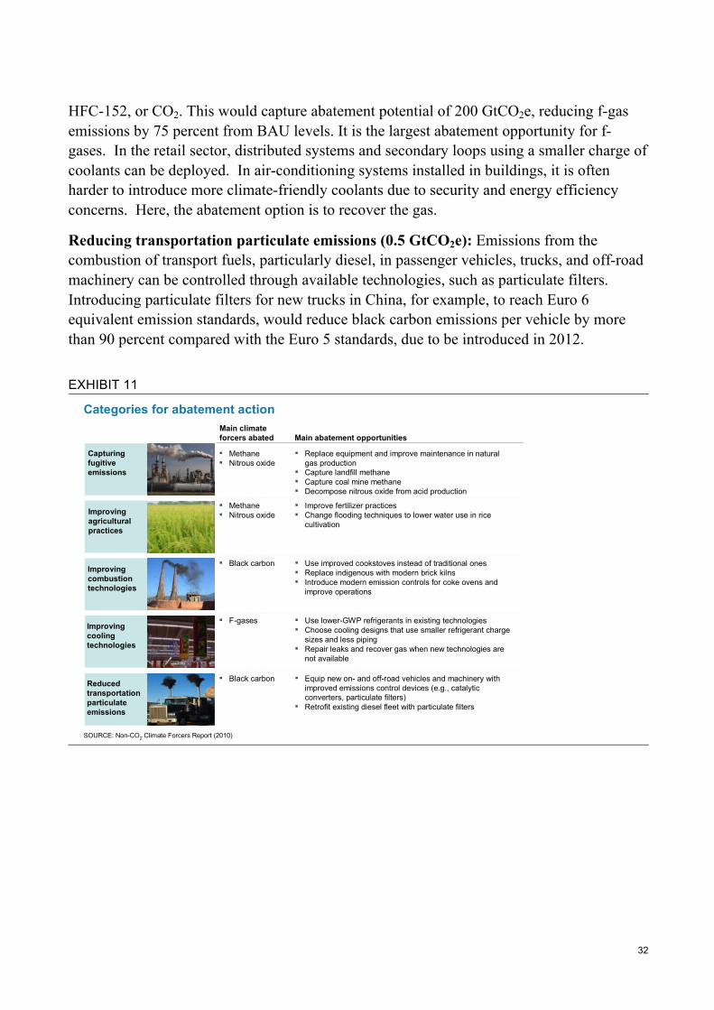
32

HFC-152, or CO2. This would capture abatement potential of 200 GtCO2e, reducing f-gas emissions by 75 percent from BAU levels. It is the largest abatement opportunity for f-gases. In the retail sector, distributed systems and secondary loops using a smaller charge of coolants can be deployed. In air-conditioning systems installed in buildings, it is often harder to introduce more climate-friendly coolants due to security and energy efficiency concerns. Here, the abatement option is to recover the gas.

Reducing transportation particulate emissions (0.5 GtCO2e): Emissions from the combustion of transport fuels, particularly diesel, in passenger vehicles, trucks, and off-road machinery can be controlled through available technologies, such as particulate filters. Introducing particulate filters for new trucks in China, for example, to reach Euro 6 equivalent emission standards, would reduce black carbon emissions per vehicle by more than 90 percent compared with the Euro 5 standards, due to be introduced in 2012.

EXHIBIT 11

Categories for abatement action

Improving agricultural practices

Improving cooling technologies


Reduced transportation particulate emissions

Improving combustion technologies

Main climate forcers abated Main abatement opportunities

▪ Methane▪ Nitrous oxide

▪ Replace equipment and improve maintenance in natural gas production

▪ Capture landfill methane▪ Capture coal mine methane▪ Decompose nitrous oxide from acid production

▪ Methane▪ Nitrous oxide

▪ Improve fertilizer practices ▪ Change flooding techniques to lower water use in rice

cultivation

▪ Black carbon ▪ Use improved cookstoves instead of traditional ones ▪ Replace indigenous with modern brick kilns▪ Introduce modern emission controls for coke ovens and

improve operations

▪ F-gases ▪ Use lower-GWP refrigerants in existing technologies▪ Choose cooling designs that use smaller refrigerant charge

sizes and less piping▪ Repair leaks and recover gas when new technologies are

not available

▪ Black carbon ▪ Equip new on- and off-road vehicles and machinery with improved emissions control devices (e.g., catalytic converters, particulate filters)

▪ Retrofit existing diesel fleet with particulate filters


33

EXHIBIT 12


Key opportunities


0.5 15.61.0

Abatement Case2030


0.7


20.1

BAUgrowth

15.8 4.3

BAUEmissions 2005

1.8


0.6

Reduced transportation particulateemissions

BAUEmissions 2030

-22%





▪ Emission controls for on-road and off-road vehicles, particularly heavy-duty diesel trucks

▪ Landfill gas capture ▪ Oxidation of coal

mine ventilationair and mine degasification▪ Electrostatic





~40% ~20% ~20% ~10% ~10%


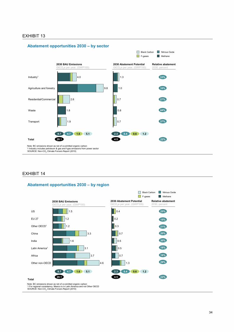
Methane, the f-gases, and black carbon have the greatest relative abatement potential. In 2030, emissions could be cut by 26 percent, 40 percent, and 24 percent respectively from BAU levels. Nitrous oxide emissions are harder to tackle, with only 8 percent abatement potential identified. Emissions would drop if fertilizers were no longer used, but that could jeopardize productivity and the ability to meet food requirements. Therefore, only relatively small changes in the amount of fertilizer used are envisaged in this report.

The waste sector is the sector with the greatest relative abatement potential as emissions can be captured relatively easily for solid waste, which is quite concentrated. The same is true for the industrial sector, which includes petroleum and gas that emits much methane from fairly concentrated sources. The agricultural sector is the sector with the highest emissions, but these are also the most difficult to abate as there are so many small emission sources. This sector thus has the smallest relative abatement potential—just 10 percent of 2030 BAU levels (Exhibit 13). Across regions relative abatement potential is fairly similar, with a higher BAU share of f-gases and black carbon in a region increasing the relative abatement potential (Exhibit 14).

34

EXHIBIT 13

Abatement opportunities 2030 – by sector

Transport 1.9

Waste 1.8

Residential/Commercial 2.6

Agriculture and forestry 9.8

Industry1 4.0

Total

2030 Abatement PotentialGtCO2e per year, (GWP100)

2030 BAU EmissionsGtCO2e per year, (GWP100)

Note: BC emissions shown as net of co-emitted organic carbon1 Industry includes petroleum & gas and f-gas emissions from power sector

44%

37%

Relative abatement2030, percent

4.5

2.3 0.4 0.6 1.2

22%20.1

8.7 4.7 1.6 5.1

33%

27%

10%

F-gases

Black Carbon

Methane

Nitrous Oxide

0.7

0.8

0.7

1.0

1.3


EXHIBIT 14

1.6

China 3.3

Other OECD1 1.2

EU 27 1.2

US 1.5

Other non-OECD 4.6

Africa 3.7

Latin America1 3.1

India

Total




1.3

0.7

0.5

0.5

0.7

0.3

0.2

0.4

21%

15%

25%

20%

30%

18%

18%

F-gases

Black Carbon

Methane

Nitrous Oxide

Abatement opportunities 2030 – by region

22%20.1

8.7 4.7 1.6 5.1

29%

Note: BC emissions shown as net of co-emitted organic carbon


4.5

2.3 0.4 0.6 1.2

1 For regional consistency, Mexico is in Latin America and not Other OECD

35

Abatement cost Half of the abatement potential identified in this report comes at a societal profit,40 meaning that initial investments would be outweighed by the subsequent economic benefits. Examples include abatement measures to capture methane gas that is then used to generate electricity, and the recovery and re-use of f-gases. Another 30 percent of the abatement potential can be captured in 2030 at up to $20/tCO2e (Exhibit 15). In general, the methane abatement measures are the least expensive and the black carbon measures the most expensive. However, the latter also deliver important health and other non-climate-related environmental benefits.

In our analysis, we did not include a monetary value for the additional benefits of abatement, such as the value of lives saved or of prevented crop losses. The cost curves show the pure project costs. Many organizations do assign a value to the prevention of premature deaths in order to calculate the cost benefit of safety and public health measures. These should be looked at on a country-by-country basis when prioritizing abatement measures.

In addition, it should be noted that the cost curve takes a societal perspective, thus taxes and subsidies are excluded and a societal interest rate is used; an individual decision-maker would face slightly different costs. Furthermore, transaction costs such as those for capacity building, education, or enforcement monitoring are excluded, as these will depend on the policies chosen to incentivize implementation.

40 See the “Study Approach” chapter for a more detailed explanation.

36

EXHIBIT 15

Abatement cost curve of non-CO2 climate forcers in 2030

80

200

3.0 4.0

Abatement cost, societal perspectiveUSD/tCO2e

-40

60

0

20

40

2.0

Abatement potentialGtCO2e per year

-60

1.00-20

F-gases

Nitrous oxide

Methane

Black carbon

2.3 GtCO2e at societal profit 1.4 GtCO2e at 0-20USD/tCO2e

0.8 GtCO2e at >20 USD/tCO2e


Landfill gas - direct use

VSBK replacing BTK & IDK

P&G upstream - equipment upgradesRice cultivation - changed nutrient management

Rice cultivation - water managementImproved cook stoves

Composting of new solid waste

Landfill gas - electricity generationMotor vehicle air conditioning systems – low-GWP refrigerants

Livestock - antimethanogen vaccineHDV diesel US 04/Euro 5 controls

2-/3-wheeler TWC

Livestock - feed supplementsAgricultural machinery, stage 2 controls

Industrial wastewater - improved treatment

HDV particulate filters, new (Euro 6)

Project cost only, value of public health and environmental benefits not included

100-year GWP

The capital investments needed to implement all the measures would be approximately $77 billion per year in 2030 (Exhibit 16). Most of this investment is required in the developing world, as this is where most abatement potential lies. The issue of how the investment will be financed is outside the scope of this report, which focuses on the technical abatement measures.

The two sectors with the greatest investment needs are transportation and waste management. In transportation, black carbon is reduced through the addition of filters and other capture technologies, and f-gas emissions are reduced by using new air conditioning systems, both of which require upfront investments, but are relatively modest compared to the cost of the car. For a light duty vehicle with a production cost of $15,000, the cost increase of moving to a low GWP air conditioning system would only be about $75 of incremental investment, or 0.5 percent of the total production cost. The waste sector capital expenditures are a result of the need to install gas capturing piping and in many cases electricity generators at landfills and onsite wastewater management systems at industrial sources.

The capital requirements may look daunting, but are less so if the net cost of the abatement measures is taken into account. For the abatement that would occur in 2030, less than 15 percent of the total capital investment is needed for those measures that will return a net profit to society – which represents 50 percent of the total abatement.

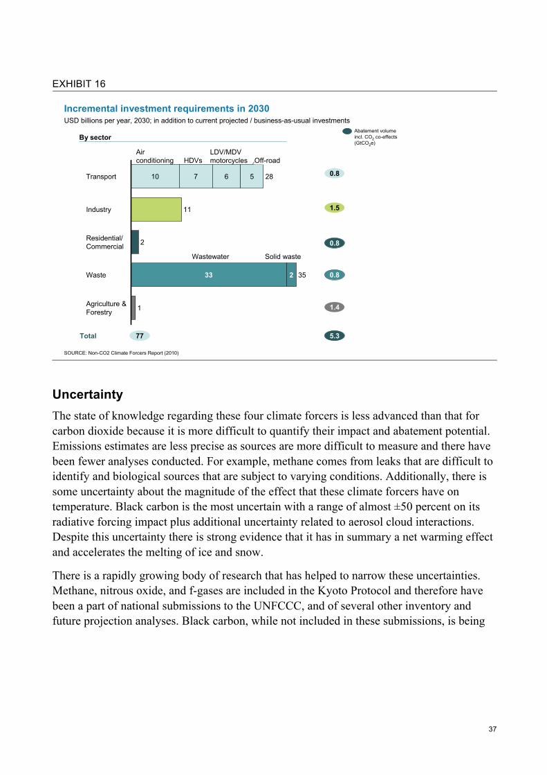
37

EXHIBIT 16

By sector

77Total

Incremental investment requirements in 2030USD billions per year, 2030; in addition to current projected / business-as-usual investments

Abatement volume incl. CO2 co-effects(GtCO2e)

0.8

Agriculture &Forestry

5

11

2

233

1

Waste 35

Residential/Commercial

Industry

Transport 2810 7 6

5.3


0.8

0.8

1.5

1.4

Solid wasteWastewater

Air conditioning

LDV/MDVmotorcyclesHDVs Off-road

Updated 100701

Uncertainty The state of knowledge regarding these four climate forcers is less advanced than that for carbon dioxide because it is more difficult to quantify their impact and abatement potential. Emissions estimates are less precise as sources are more difficult to measure and there have been fewer analyses conducted. For example, methane comes from leaks that are difficult to identify and biological sources that are subject to varying conditions. Additionally, there is some uncertainty about the magnitude of the effect that these climate forcers have on temperature. Black carbon is the most uncertain with a range of almost ±50 percent on its radiative forcing impact plus additional uncertainty related to aerosol cloud interactions. Despite this uncertainty there is strong evidence that it has in summary a net warming effect and accelerates the melting of ice and snow.

There is a rapidly growing body of research that has helped to narrow these uncertainties. Methane, nitrous oxide, and f-gases are included in the Kyoto Protocol and therefore have been a part of national submissions to the UNFCCC, and of several other inventory and future projection analyses. Black carbon, while not included in these submissions, is being

38

actively studied by several leading researchers41 with a number of publications in 2011 and 2012.

Some have argued that there are too many uncertainties surrounding those non-CO2 climate forcers for policymakers to take any decisive action. However, the conclusion of this research is that the uncertainties involved do not detract from the main findings. Non-CO2 climate forcers cause a substantial portion of global warming (at least 25 percent, but likely closer to 30 percent) and black carbon and methane increase air pollution and consequential disease and premature mortality. Furthermore a range of abatement measures exists that can be quantified (at least 3.5 GtCO2e of abatement potential, but likely over 5 GtCO2e) to capture both climate and associated public health benefits.

That said, it is important to understand how the uncertainties might impact the more detailed analysis. To account for those, a Monte Carlo analysis was performed to assess the expected value and variation for the baseline emissions (expressed in CO2e) and the abatement potential in 2030.

The major areas of uncertainty are:

Emissions inventory: The difficulty in measuring emissions arises from both a lack of global data and the nature of the emissions. Human-induced CO2 largely results from burning fossil fuels, which directly correlates with CO2 emissions, and for which fuel consumption is measured. Non-CO2 forcers, however, often leak into the atmosphere or result from incomplete combustion processes, making it more difficult to measure emissions or even identify all the sources. In this analysis, the uncertainty bands from the US EPA 2010 United States Inventory of Emissions42 are used for methane, nitrous oxide, and f-gases. For example, the inventory range for nitrous oxide is from about 10 percent lower to nearly 50 percent higher emissions. This EPA source likely underestimates the range of uncertainty as global emissions measurements are more difficult to obtain compared to those for the United States. The uncertainty bands for the black carbon inventory are those used by Bond et al.43 Please see Appendix E for areas of suggested further scientific research that would reduce inventory uncertainty.

Global warming impact: Sophisticated climate models exist to understand the impact that human-induced emissions have on the climate. Scientists use these models to derive the GWP values that allow them to compare the global warming impact of the different climate forcers (see also the chapter “Study Approach – Climate Metrics”), but there is still uncertainty around these numbers. This report uses the uncertainty bands for methane, nitrous oxide, and the f-gases from the IPCC’s Fourth Assessment Report at ±35 percent of

41 See for example, Bond (2007); IIASA GAINS model; and Fuglestvedt (2009). 42 US EPA (2010). 43 Bond et al. (2007).

39

the 100-year GWP value for these greenhouse gases.44 For black carbon, whose climatic effects are less well understood, recent 100-year GWP estimates range from 200 to 1500.45 The GWP value used in this report, of 917, falls in the mid-range of these estimates, where recent studies, including the ongoing assessment “Bounding the Role of Black Carbon in Climate,”46 seem to converge. The 95 percent confidence interval for black and organic carbon is still under scientific discussion, but for this analysis we have used an uncertainty band for the GWP for black carbon of 490 to 1350, where the most common values lie.

Implementation share: The extent to which emissions can be reduced depends on technical feasibility and costs, which in turn determine the percentage of an activity that can be changed through implementation of the abatement measure. It also depends on the skill and ambitions of the program and individuals. The abatement potential in this report is based on technical implementation shares used in previous assessments made by the US EPA, by IIASA, by the Technology and Economic Assessment Panel of the Montreal Protocol (TEAP), by McKinsey & Company; and by expert panels formed for this report.

Together, these three major areas of uncertainty can have a significant impact on the total abatement potential. The first two suggest that this report likely underestimates BAU emission levels. This is for two reasons. First, because of the nature of the emissions, many are likely to be overlooked. Second, this report uses the IPCC’s Second Assessment report 100-year GWP values for methane, nitrous oxide, and f-gases, as these are still widely used. However, these GWP values are lower than those in the IPCC’s more recent Fourth Assessment report – which means that on average the impact of these emissions on the global climate are underestimated. Adjusting for these two factors would raise BAU emission levels by 22 percent (Exhibit 17). The full range is from about 25 percent lower to nearly 95 percent greater than the value of 20.1 GtCO2e identified in the main text. Additionally, the analysis indicates that there is a less than 15 percent probability that emissions in 2030 would be less than 20 GtCO2e under business-as-usual. This implies that non-CO2 forcers contribute at least 25 percent, but more likely 30 percent to global warming in 2030.

44 In the main analysis, we use the GWP values from the Second Assessment Report in order to make our report comparable with

other reports, which though still within the bands of uncertainty are not the expected values. 45 Bond et al., 2005; Bond, 2007; Boucher and Reddy, 2008; and Rypdal et al., 2009. 46 A study is currently underway which will further narrow the uncertainty around the global warming potential of black carbon.

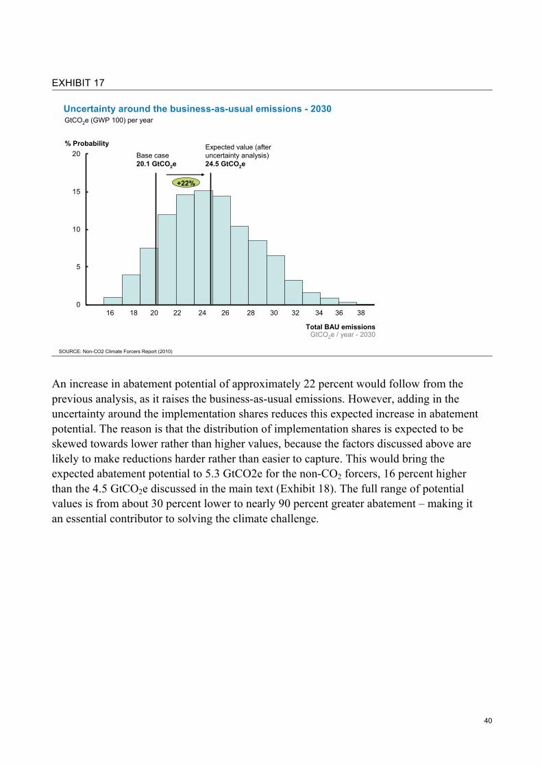
40

EXHIBIT 17

Uncertainty around the business-as-usual emissions - 2030


0

5

10

15

20

Total BAU emissionsGtCO2e / year - 2030

% Probability Expected value (afteruncertainty analysis)24.5 GtCO2e

Base case20.1 GtCO2e

+22%


16 18 20 3422 24 26 28 30 32 36 38

Updated 100701Abhishek

An increase in abatement potential of approximately 22 percent would follow from the previous analysis, as it raises the business-as-usual emissions. However, adding in the uncertainty around the implementation shares reduces this expected increase in abatement potential. The reason is that the distribution of implementation shares is expected to be skewed towards lower rather than higher values, because the factors discussed above are likely to make reductions harder rather than easier to capture. This would bring the expected abatement potential to 5.3 GtCO2e for the non-CO2 forcers, 16 percent higher than the 4.5 GtCO2e discussed in the main text (Exhibit 18). The full range of potential values is from about 30 percent lower to nearly 90 percent greater abatement – making it an essential contributor to solving the climate challenge.

41

EXHIBIT 18

Uncertainty around the abatement potential for non-CO2 forcers– 2030


0

5

10

15

20

Abatement potentialGtCO2e / year

% Probability Expected value (afteruncertainty analysis)5.3 GtCO2e

Base case4.5 GtCO2e

+16%


3 4 5 6 7 8

NEEDS UPDATING –Abhishek please use this format


The cost of abatement, which is driven by factors such as capital costs, is also uncertain. In general, almost all cost assumptions are specific to individual abatement measures and any changes in input costs do not have a large impact on the overall results. The major exceptions to this are energy prices and societal interest rates, to which the analysis is quite sensitive. Many abatement levers either save fuel, such as natural gas equipment replacements, or use more fuel, such as some off-road vehicle particulate control measures. A 50 percent increase in energy prices results in a 30 percent reduction in the average cost of abatement from baseline levels going from about $11/tCO2e down to $8/tCO2e. Higher energy prices lead to a lower cost of abatement because of the sales value of methane and fuel savings in some black carbon and f-gas abatement.

Changes to the interest rate likewise have a strong impact on the cost of abatement. If interest rates go up to 10 percent from 4 percent, closer to investor interest rates, emissions reduction measures with large capital costs become more expensive. The average cost of abatement rises about 75 percent with such an increase, to nearly $20/tCO2e.

The major implications of this uncertainty analysis are, first, that it is likely that we have underestimated the size of the overall emissions, which would increase their importance in global temperature stabilization discussions. Second, it is likely that a lower percentage, but a higher absolute value, of emissions will technically be able to be reduced. Costs will change significantly if key externalities such as energy prices change; however, changes in individual lever costs only marginally impact overall findings. Consequently, the

42

uncertainties are not such that they would change the basic findings of the report – there is

enough known now to support action.

Reducing non-CO2 emissions is essential to limit global warming during this century, slow the rate of temperature increase, and reduce the risk of adverse climate feedbacks

There are three angles from which to assess the need for urgency to reduce the non-CO2 climate forcers in parallel to carbon dioxide. The first is the need to limit global warming, given that many governments and scientists have agreed on 2 degrees Celsius as the maximum acceptable increase.47 The second is the need to reduce the rate of temperature increase as this rate influences the ability of ecosystems to adapt.48 The third is the need to reduce the risk of adverse climate feedbacks on both a global and regional scale. One example of an adverse climate feedback is accelerated Arctic melting, which would further speed up temperature increases.

Ultimately, long-term temperature increases and temperature stabilization levels after mitigation will be determined by the level and pathway of carbon dioxide emissions, the most prevalent GHG. Still, abating non-CO2 climate forcers in parallel to CO2 is essential to achieving temperature stabilization at all. Even assuming no growth in non-CO2 emissions after 2030, there would be about 20 GtCO2e of emissions without abatement. This amount represents nearly all of, if not more than, the total emissions per year that could be perpetually emitted without further increasing the temperature, i.e., the level that would enable temperature stabilization. No abatement of the non-CO2 forcers would essentially mean that CO2 emissions would need to be cut close to zero in order to achieve stabilization.

In the short term, non-CO2 abatement has an even greater impact on slowing the rate of temperature increase, due to the high short-term warming effect of those climate forcers. The IPCC has concluded with high confidence that temperature increases are already occurring and having an effect on ecosystems.49 Evidence includes glacial melting rates, earlier “greening” of vegetation, shifts in plant and animal ranges towards the poles and to high altitudes, and changes in aquatic life associated with warmer ocean temperatures. The rate of change in local climate has implications for the ability of those ecosystems to adapt: the faster the change, the lower the ability to adapt, and the higher the risk of irreversible changes. Berntsen et al. demonstrated that drastically reducing non-CO2 climate forcers in the short term prolongs the time to reach maximum temperatures by several decades –

47 See e.g., Copenhagen Accord, 2009. 48 Root et al., 2003. 49 IPCC AR4, 2007.

43

slowing the rate of change, thus improving the ability to adapt.50 Van Vuuren et al. confirm this finding and conclude that multi-gas abatement scenarios are also the most cost-effective way to contain warming.51

Moreover, reducing black carbon would help alleviate non-temperature-related climate changes, such as the melting of glaciers and arctic ice through changes in surface reflectivity. This melting would otherwise accelerate the rate of temperature change by exposing darker surfaces underneath and also contributes to potential sea level increases. Abating methane, which as a precursor of tropospheric ozone damages vegetation, would improve the ability of plants to sequester carbon.52 These are both areas where abatement would substantially reduce adverse climate feedbacks.53

On top of the positive climate effects, 80 percent of the measures also improve public health and half come at a net savings to society

Reducing methane and black carbon emissions will deliver near-term health benefits. Nearly 80 percent of the abatement measures result in air pollution reduction, thereby improving public health (Exhibit 19). The remaining 20 percent of the abatement measures can be divided into those that result in a net societal savings (such as refrigerant leak prevention) and those that are purely climate change mitigation measures (such as industrial nitrous oxide controls). Overall, half of the measures come at societal profit, independent of whether the motivation to pursue them is improved public health or purely climate change.

50 Berntsen et al., CICERO, 2010. Temperature increase target set at 1.5°C warming. In the case of the same abatement for all

climate forcers maximum temperature is reached after 50 years (1.5% p.a. rate of temperature increase); whereas in the case of drastic non-CO2 reduction it takes 80 years (1.0% p.a.).

51 Van Vuuren et al., 2006. Including non-CO2 gases is crucial to the formulation of a cost-effective abatement response, and can reduce costs by 30-40 percent compared to a CO2 only reduction strategy for the same radiative forcing target.

52 Royal Society, 2008. 53 Lenton, 2008.

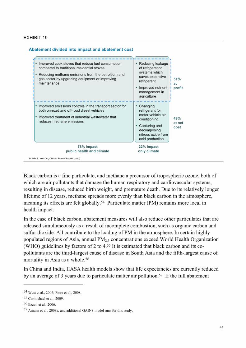
44

EXHIBIT 19

Abatement divided into impact and abatement cost


51%at profit

49%at netcost

78% impactpublic health and climate

22% impactonly climate

▪ Improved cook stoves that reduce fuel consumption compared to traditional residential stoves

▪ Reducing methane emissions from the petroleum and gas sector by upgrading equipment or improving maintenance

▪ Improved emissions controls in the transport sector for both on-road and off-road diesel vehicles

▪ Improved treatment of industrial wastewater that reduces methane emissions

▪ Reducing leakage of refrigeration systems which saves expensive refrigerant

▪ Improved nutrient management in agriculture

▪ Changing refrigerant for motor vehicle air conditioning

▪ Capturing and decomposing nitrous oxide from acid production

Updated 100706

Black carbon is a fine particulate, and methane a precursor of tropospheric ozone, both of which are air pollutants that damage the human respiratory and cardiovascular systems, resulting in disease, reduced birth weight, and premature death. Due to its relatively longer lifetime of 12 years, methane spreads more evenly than black carbon in the atmosphere, meaning its effects are felt globally.54 Particulate matter (PM) remains more local in health impact.

In the case of black carbon, abatement measures will also reduce other particulates that are released simultaneously as a result of incomplete combustion, such as organic carbon and sulfur dioxide. All contribute to the loading of PM in the atmosphere. In certain highly populated regions of Asia, annual PM2.5 concentrations exceed World Health Organization (WHO) guidelines by factors of 2 to 4.55 It is estimated that black carbon and its co-pollutants are the third-largest cause of disease in South Asia and the fifth-largest cause of mortality in Asia as a whole.56

In China and India, IIASA health models show that life expectancies are currently reduced by an average of 3 years due to particulate matter air pollution.57 If the full abatement 54 West et al., 2006; Fiore et al., 2008. 55 Carmichael et al., 2009. 56 Ezzati et al., 2006. 57 Amann et al., 2008a, and additional GAINS model runs for this study.

45

potential of black carbon were captured in China and India, life expectancies in 2030 in these countries could be increased by an average of 2 to 4 months per person. These numbers are for outdoor air pollution reductions only. If the impact that these measures have on indoor air pollution were included, the resulting life expectancy increases would be larger.

Tropospheric ozone, to which methane is a precursor in the atmosphere, causes a variety of diseases such as reduced lung function, respiratory symptoms, and airway inflammation,58 thus contributing to morbidity. Some health studies have also identified a link between methane and mortality, although the strength of the connection is under scientific debate.59 If the connection is as strong as West and Fiore 60 state, achieving the targeted global reductions in methane emissions (2.3 GtCO2e in 2030 compared with BAU levels) would prevent over 30,000 premature mortalities per year in 2030.61

We did not attach a monetary value to the potential lives saved; however, the following could be considered for context. The average cost to save a life through the abatement of methane emissions identified in this report would be $900,000 per reduced premature death. This is within the bounds of many national and insurance values that are used to estimate cost efficiency of life-saving measures.62 Since the mortality rate for particulate matter is higher, the cost to save a life could be even lower when reducing black carbon emissions. (More detail on the health benefit methodology can be found in the "Study Approach – Health benefits" chapter.)

Improved health at such a scale would also help the economy as a result of fewer days missed from work and lower healthcare costs.

There are further environmental benefits, which are not climate related, to the reduction of the non-CO2 climate forcers. These include the safeguarding of water resources, higher crop yields, healthier forests, and less use of fossil fuels—which improves energy security.

In the case of black carbon, for example, abatement would help preserve vital water supplies by reducing the rate at which glaciers melt in the springtime. At certain times of the year, faster melting can cause floods as reservoirs are overwhelmed. At other times there may be water shortages as many people currently rely on the gradual melting of the glaciers for their

58 Royal Society, 2008; Smith, K., 2009. 59 The link between methane and mortality assumes that 1) methane contributes to all ozone concentrations and not just background


60 West et al., 2006; Fiore et al., 2008. 61 It will take a number of years before the tropospheric ozone levels drop as a result of the methane abatement. Therefore, the

reduced premature mortalities per year would be almost doubled by 2050 if the abatement is sustained. 62 Miller, 2000.

46

water. See the chapter on black carbon in this report for a more detailed explanation of how black carbon impacts snow and ice.

Tropospheric ozone, caused in part by methane emissions, impairs the growth of forests and agricultural crops, reducing yields and nutritional quality.63 The annual global cost of crop losses due to ozone was estimated at between $14 billion and $16 billion in the year 2000 for rice, soybean, maize, and wheat combined.64

The improved agricultural practices identified in this report to reduce global warming will also reduce potential harm to the surrounding environment. For example, the more efficient use of both mineral fertilizers and manure would reduce the amount of nutrients that seep into waterways, thereby reducing both the formation of algae blooms that kill fish and make the water undrinkable, and the contamination of groundwater.

While a large share of the measures is relatively straightforward to implement, capturing the remainder will be challenging as millions of people would need to take action, some of whom are among the world’s poorest

Reducing emissions of non-CO2 forcers is comparatively straightforward. In many cases, there is little infrastructure “lock in” since emissions sources such as refrigerators and diesel engines are replaced every 10 to 15 years. In cases of large capital-intensive assets, such as coal mines or landfills, there are “end of pipe” technologies available that do not require stock replacement. Moreover, the technology is largely already available, well understood, and relatively simple.

The major technical advancement still needed to capture the abatement potential identified in this report is the commercialization of vaccines for reducing enteric fermentation. Other, newer technologies that could deliver additional abatement potential have not been included due to lack of sufficient proof of concept. These include additional alternative methods to reduce enteric fermentation, new fertilizers or systems that increase crop uptake of nitrogen, and systems to capture black carbon emissions from shipping.

However, there are still implementation challenges that remain:

Upfront investment: Many of the abatement measures require initial capital that might prove difficult to secure. The global investment needed for the full mitigation potential is $77 billion per year in 2030. Companies everywhere often choose not to invest their limited resources in activities that are not core to their central business or do not meet internal investment hurdle rates, even if the investments would generate value in the longer term. The added complication here is that over 90 percent of the investments needed to reduce non-CO2 forcers are needed in the developing world, where resources are even more limited. 63 Royal Society, 2008. 64 van Dingenen et al., 2009.

47

Many of the world’s poorest people will need to invest in cleaner technologies if the full abatement potential identified in this report is to be captured. Individual families, rural farmers, and family-run businesses will have significant difficulty in amassing the capital needed for new appliances, retrofits for equipment, or alternative fertilizers. Governments interested in pursuing these abatement measures will have to devise both regulatory and fiscal policies to address these challenges. Though securing financing will be difficult, it is worth noting that less investment per tonne of abatement is required for the non-CO2 climate forcers than for CO2.

Net costs: One half of the abatement potential is at net cost to consumers and businesses in the societal perspective, meaning that investments or operational costs will not be recouped though energy or water savings, for example. Because of the health implications of many of the abatement opportunities, they would likely have already been implemented if governments and citizens were able to afford them. In order to secure this abatement potential, long-term incentives or regulations will be needed to encourage the necessary investments.

Institutional capacity and fragmentation: Many of the sources of non-CO2 emissions are relatively small and diffuse, such as residential stoves and farmlands, creating a significant implementation challenge. The non-CO2 forcer abatement potential already takes into account that a portion of such sources will remain stubbornly out of reach. Capturing the remainder will be no less a challenge, as a majority of the abatement opportunity is in the developing world, where regulatory and educational institutions are often not as strong. These countries will need to develop regulatory expertise to set standards, and enforce as well as monitor progress towards goals, such as those for industrial mandates. For other measures, such as in agriculture, the expertise and capacity to educate thousands of people on emissions abatement measures will need to be built up. Many of these opportunities are positive investment opportunities, as in cases where it is feasible to use nutrient management techniques in croplands and grasslands to reduce fertilizer use. However, subsistence farmers might be understandably reluctant to change the way they farm, unless they can be shown there is little risk involved. To overcome such barriers, large-scale educational programs will be required and perhaps even crop guarantee schemes.

Awareness: Individuals, companies and even governments are often unaware of the full environmental and climate impact of their non-CO2 forcer emissions. Building such awareness will be important to sustaining new public policies and the active cooperation of owner/operators of non-CO2 emission sources. It will be particularly challenging to raise awareness among populations spread throughout rural areas, where many of the abatement opportunities lie.

48


Carbon dioxide accounts for more than half of global warming. Its atmospheric concentration has risen 35 percent since 1750 and is now at about 390 ppmv, the highest level in 800,000 years. Annual CO2 emissions must be reduced more than 80 percent to stabilize carbon dioxide concentrations in the atmosphere. If global CO2 emissions peak in the next decade and fall to 50-85 percent of 2000 levels by 2050, global mean temperature increases could be limited to 2.0-2.4°C above pre-industrial levels.65 The need for CO2 reductions is urgent. Even a few years' delay in the peak can mean the world is committed to a significantly higher temperature rise than would otherwise be the case - for every ten years the peak is postponed, another half degree of temperature increase becomes unavoidable.66

Non-CO2 mitigation measures will not eliminate the need for massive CO2 reductions but can ease the pathway to long-term climate stabilization. Non-CO2 measures will slow the rate of temperature change over the next several decades. The near and mid-term benefits of non-CO2 abatement will also reduce the risk of triggering irreversible tipping points in the earth’s climate system and capture public health benefits. Combining CO2 and non-CO2 strategies, therefore, offers the greatest chance of achieving the limitation to 2 degrees Celsius warming adopted in the Copenhagen Accord.

65 Climate Stabilization Targets: Emissions, Concentrations, and Impacts over Decades to Millennia (2011), National Research Council. 66 Dr. Vicky Pope, Hadley Centre Director of Climate Change (2009).

49

Non-CO2 climate forcer perspectives

Black Carbon Black carbon, commonly known as a component of soot, is an aerosol—that is, a small, solid particle in the atmosphere. Because it is black, it is much more effective at absorbing energy than CO2 and hence a more potent climate-forcing agent despite a much shorter lifetime. Black carbon is emitted when the carbon in a given carbonaceous fuel fails to get fully converted into CO2, a process known as incomplete combustion.

Climate Effects of Black Carbon

Black carbon contributes to climate change in three main ways:

■ Light absorption: Black carbon particles warm the atmosphere by absorbing sunlight and then emitting that energy as radiation (heat), warming the surrounding air. This effect is considered a "direct effect" of black carbon on the climate. The 100-year global warming potential (GWP) of this direct effect is 864 times as great as that of CO2, based on Rypdal et al., 2009.1 For a more detailed discussion of the GWP value, see the “Uncertainty” section in the chapter “Global Perspective.”

■ Snow albedo: Black carbon particles that are deposited on snow and ice decrease albedo—that is, they darken the surface and reduce reflectivity, amounting to an additional global average 100-year GWP of 53.1 This has two effects: first, the reduced reflectivity of snow and ice increases the rate at which they melt because more sunlight is absorbed, particularly during spring. Black carbon is believed to be among the most important causes of arctic melting, and may contribute as much to the melting of snow packs and glaciers in the Himalayas as does CO2.1 Second, the melting snow and ice unveils darker surfaces, such as rocks, soils, or ocean water that absorb yet more light and so raise atmospheric temperatures, further accelerating melting.

■ Cloud effect: Black carbon affects the climate indirectly through its interaction with clouds. Soot particles in cloud droplets increase absorption of light, which, when released as radiation, may cause clouds to shrink and raise temperatures. On the other hand, small particles, particularly those that are water-soluble such as the sulfates that are co-emitted with black carbon, can cause the formation of more but smaller cloud droplets. This increases a cloud’s reflectivity and prolongs its life, which has a cooling effect. However, as the overall effect of these interactions is still not well understood, the total GWP of black carbon as used in this study does not include cloud effects.

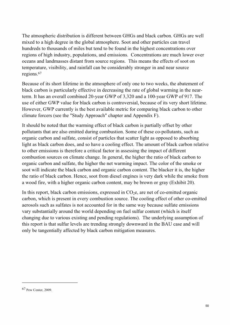
50

The atmospheric distribution is different between GHGs and black carbon. GHGs are well mixed to a high degree in the global atmosphere. Soot and other particles can travel hundreds to thousands of miles but tend to be found in the highest concentrations over regions of high industry, populations, and emissions. Concentrations are much lower over oceans and landmasses distant from source regions. This means the effects of soot on temperature, visibility, and rainfall can be considerably stronger in and near source regions.67

Because of its short lifetime in the atmosphere of only one to two weeks, the abatement of black carbon is particularly effective in decreasing the rate of global warming in the near-term. It has an overall combined 20-year GWP of 3,320 and a 100-year GWP of 917. The use of either GWP value for black carbon is controversial, because of its very short lifetime. However, GWP currently is the best available metric for comparing black carbon to other climate forcers (see the "Study Approach" chapter and Appendix F).

It should be noted that the warming effect of black carbon is partially offset by other pollutants that are also emitted during combustion. Some of these co-pollutants, such as organic carbon and sulfate, consist of particles that scatter light as opposed to absorbing light as black carbon does, and so have a cooling effect. The amount of black carbon relative to other emissions is therefore a critical factor in assessing the impact of different combustion sources on climate change. In general, the higher the ratio of black carbon to organic carbon and sulfate, the higher the net warming impact. The color of the smoke or soot will indicate the black carbon and organic carbon content. The blacker it is, the higher the ratio of black carbon. Hence, soot from diesel engines is very dark while the smoke from a wood fire, with a higher organic carbon content, may be brown or gray (Exhibit 20).

In this report, black carbon emissions, expressed in CO2e, are net of co-emitted organic carbon, which is present in every combustion source. The cooling effect of other co-emitted aerosols such as sulfates is not accounted for in the same way because sulfate emissions vary substantially around the world depending on fuel sulfur content (which is itself changing due to various existing and pending regulations). The underlying assumption of this report is that sulfur levels are trending strongly downward in the BAU case and will only be tangentially affected by black carbon mitigation measures.

67 Pew Center, 2009.

51

EXHIBIT 20

Ratio of black carbon to organic carbon

3.8

1.81.3

0.70.20.1

Road transportOff-road transport

Residen-tial coal

Industry and power

Residential biomass

Open burning

Soot from diesel combustion appears black because of its high content of black carbon, the light-absorbing component of aerosols

Smoke from open burning of biomass or wildfires appears gray because of the high ratio of OC which scatters sunlight and therefore appears light colored

Note: All sources emit significant quantities of other pollutants that may warm or cool the climate, including CO2 (warming), NOx (ozone and N2Owarming, nitrate cooling), and SO2 (sulfate cooling)SOURCE: Non-CO2 Climate Forcers Report (2010), Bond (2007), GAINS

Updated 100702

Emission sources All fuel combustion is subject to varying temperatures that result in the production of soot and smoke—a mix of small particles containing black carbon, organic carbon, and smaller amounts of sulfur and other chemicals. These emissions are known as aerosols. Black carbon comes from:

■ Contained combustion, which occurs in three main areas, each contributing around 25 percent of the net warming effect of black and co-emitted organic carbon. The largest area is transportation, due to emissions from diesel-engine road vehicles, off-road machinery, and shipping. The second is burning of coal and biomass in industry, for example in brick kilns or coke ovens. The third is emissions in the residential sector, e.g., from solid biomass combustion in cookstoves.

■ Open biomass burning is the largest source of black carbon emissions overall. However, due to the high share of co-emitted organic carbon that counters the global warming impact of black carbon, the net warming impact from this source is relatively low. It is therefore not the focus of this report. However, when black carbon from open biomass burning reaches snow- and ice-covered regions, it has the same important, indirect climate impact as emissions from contained combustion. Studies have shown that the open burning of agricultural waste in Eastern Europe and Russia, for example,

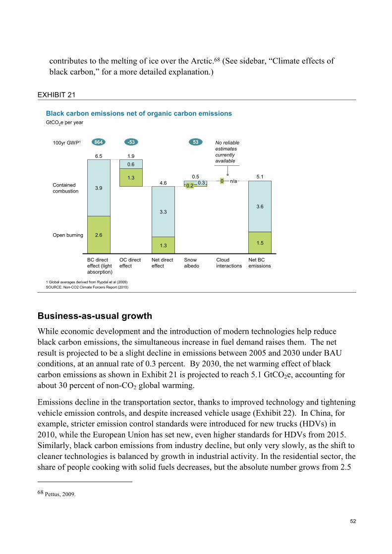
52

contributes to the melting of ice over the Arctic.68 (See sidebar, “Climate effects of black carbon,” for a more detailed explanation.)

EXHIBIT 21

Black carbon emissions net of organic carbon emissions

3.9

Net direct effect

4.6 0.2 0.3

Snowalbedo

0.50 n/a

BC directeffect (lightabsorption)

6.5

1.3

0.6

OC direct effect

1.9

1.3

3.3

2.6

Cloudinteractions

5.1

3.6

1.5

Contained combustion

Open burning

Net BC emissions

864100yr GWP1 53

1 Global averages derived from Rypdal et al (2009)

No reliable estimates currently available

GtCO2e per year

-53


Business-as-usual growth While economic development and the introduction of modern technologies help reduce black carbon emissions, the simultaneous increase in fuel demand raises them. The net result is projected to be a slight decline in emissions between 2005 and 2030 under BAU conditions, at an annual rate of 0.3 percent. By 2030, the net warming effect of black carbon emissions as shown in Exhibit 21 is projected to reach 5.1 GtCO2e, accounting for about 30 percent of non-CO2 global warming.

Emissions decline in the transportation sector, thanks to improved technology and tightening vehicle emission controls, and despite increased vehicle usage (Exhibit 22). In China, for example, stricter emission control standards were introduced for new trucks (HDVs) in 2010, while the European Union has set new, even higher standards for HDVs from 2015. Similarly, black carbon emissions from industry decline, but only very slowly, as the shift to cleaner technologies is balanced by growth in industrial activity. In the residential sector, the share of people cooking with solid fuels decreases, but the absolute number grows from 2.5

68 Pettus, 2009.

53

billion in 2005 to 2.7 billion by 2030 due to population growth.69 The net result keeps emissions close to constant. Emissions from the open burning of biomass are expected to decrease slightly due to less deforestation.

EXHIBIT 22

Net black carbon business-as-usual emissions


▪ Diesel road transport ▪ Construction & agricultural

machinery/vehicles

1.0

-0.2

-0.3

-0.9

-0.3Total

1 Net 100-year GWP of BC and OC emissions, cooling effect of SO2 not includedSOURCE: Non-CO2 Climate Forcers Report (2010); Bond inventory; Michael Walsh transport model; IIASA GAINS

Primary emission sources

▪ Coal combustion in low-tech brick kilns

▪ Coke production

▪ Solid fuel combustion in residential cookstoves

▪ Agricultural waste burning

▪ Forest/savannah firesForestry

Waste


Industry

Transport

2030

5.1

1.3

0.3 0

1.5

0.9

1.2

2005

5.6

1.4

0.2 0

1.4

1.0

1.5

0.1

▪ Open burning of waste

0.5

Net GtCO2e (GWP100) of BC and OC per year1

Agriculture

From a regional perspective, emissions are fast declining in the EU and US, at 2.8 and 2.1 percent annually, respectively. Emissions in China, Latin America, and other non-OECD countries are also decreasing, but at a much slower pace of 0.2 to 1.1 percent annually. In Africa and India, the opposite is true. Population and economic growth outpace the emissions savings achieved in the BAU case, so that emissions are expected to grow at 0.4 percent annually in Africa, and 1.0 percent annually in India.

Abatement Potential Abatement potential exists in all sectors, amounting to a total of 1.2 GtCO2e, representing 24 percent abatement of BAU emissions in 2030. Most reduction potential lies in the developing world because of the concentration of BAU emissions and scope to introduce cleaner technologies there. Looked at by sector, abatement potential is equally spread across the residential, industrial, and transportation sectors, each contributing about one third of the abatement potential (Exhibit 23). Overall, abatement in industry comes at a societal profit, 69 See IEA WEO 2006.

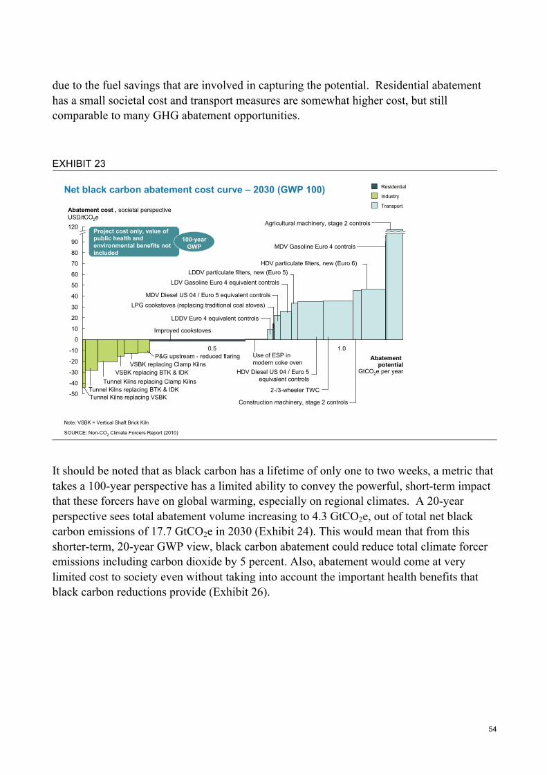
54

due to the fuel savings that are involved in capturing the potential. Residential abatement has a small societal cost and transport measures are somewhat higher cost, but still comparable to many GHG abatement opportunities.

EXHIBIT 23

Net black carbon abatement cost curve – 2030 (GWP 100)

1.0Abatement

potentialGtCO2e per year

80

0.5

-30

10

0

30

20

40

-40

-50

-10

50

Abatement cost , societal perspectiveUSD/tCO2e

70

60

-20

90

120

Note: VSBK = Vertical Shaft Brick Kiln

Industry

Residential

Transport


Tunnel Kilns replacing BTK & IDKTunnel Kilns replacing VSBK

Tunnel Kilns replacing Clamp KilnsVSBK replacing BTK & IDK

VSBK replacing Clamp KilnsP&G upstream - reduced flaring

Improved cookstoves

Use of ESP in modern coke oven

LDDV Euro 4 equivalent controls

LPG cookstoves (replacing traditional coal stoves)MDV Diesel US 04 / Euro 5 equivalent controls

LDV Gasoline Euro 4 equivalent controlsLDDV particulate filters, new (Euro 5)

HDV Diesel US 04 / Euro 5equivalent controls

2-/3-wheeler TWC

Construction machinery, stage 2 controls


MDV Gasoline Euro 4 controls

Agricultural machinery, stage 2 controlsProject cost only, value of public health and environmental benefits not included

100-year GWP

It should be noted that as black carbon has a lifetime of only one to two weeks, a metric that takes a 100-year perspective has a limited ability to convey the powerful, short-term impact that these forcers have on global warming, especially on regional climates. A 20-year perspective sees total abatement volume increasing to 4.3 GtCO2e, out of total net black carbon emissions of 17.7 GtCO2e in 2030 (Exhibit 24). This would mean that from this shorter-term, 20-year GWP view, black carbon abatement could reduce total climate forcer emissions including carbon dioxide by 5 percent. Also, abatement would come at very limited cost to society even without taking into account the important health benefits that black carbon reductions provide (Exhibit 26).

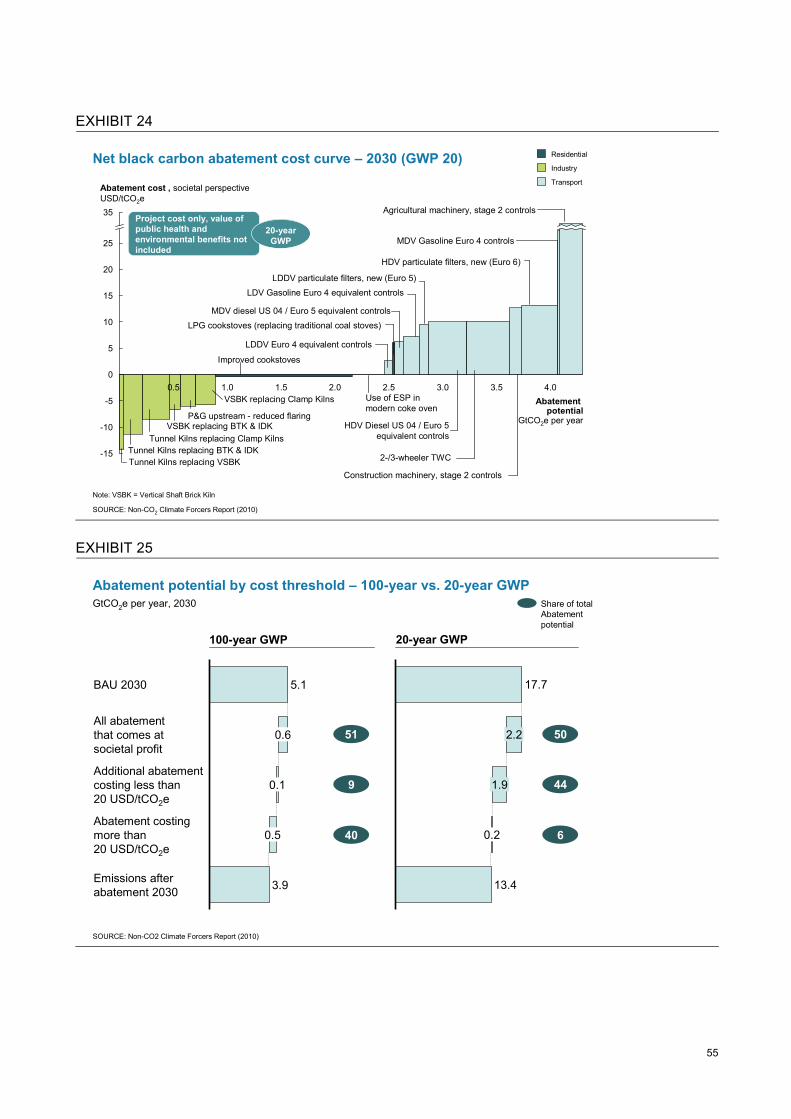
55

EXHIBIT 24

Net black carbon abatement cost curve – 2030 (GWP 20)

4.03.53.00.5

15

1.00

10

-5

25

-10

Abatement cost , societal perspectiveUSD/tCO2e35

Abatement potential

GtCO2e per year

5

20

-15

2.52.01.5


Transport

Residential

Industry


Tunnel Kilns replacing BTK & IDKTunnel Kilns replacing VSBK

Tunnel Kilns replacing Clamp KilnsVSBK replacing BTK & IDK

P&G upstream - reduced flaring

VSBK replacing Clamp Kilns

Improved cookstoves



LPG cookstoves (replacing traditional coal stoves)MDV diesel US 04 / Euro 5 equivalent controls

LDV Gasoline Euro 4 equivalent controlsLDDV particulate filters, new (Euro 5)

HDV Diesel US 04 / Euro 5equivalent controls

2-/3-wheeler TWC




Agricultural machinery, stage 2 controlsProject cost only, value of public health and environmental benefits not included

20-year GWP

EXHIBIT 25

Abatement potential by cost threshold – 100-year vs. 20-year GWPGtCO2e per year, 2030


Abatement costingmore than20 USD/tCO2e

Emissions after abatement 2030 3.9

0.6

0.5

BAU 2030

Additional abatementcosting less than20 USD/tCO2e

5.1

0.1

All abatementthat comes atsocietal profit

2.2

13.4

17.7

0.2

1.9

100-year GWP 20-year GWP

51

9

40

50

44

6

Share of totalAbatementpotential

56

The technical abatement levers can be grouped into six areas:

Improved cookstoves: The replacement of traditional residential cookstoves with ones that consume less fuel is the measure with the largest abatement potential, 0.4 GtCO2e in 2030 (using the 20-year GWP: 1.3 GtCO2e). Stoves are also being developed that increase the combustion temperature so that still fewer particles are emitted, though this additional potential has not been included in the cost curve due to inconclusive data. The improved cookstove measure comes at an average societal profit of about $1/tCO2e due to reduced coal consumption (using 20-year GWP: close to $0/tCO2e). However, if the biomass saved from using modern stoves is also assigned a monetary value—a value that derives largely from the time saved gathering wood—these cookstoves would return an even higher societal profit over their lifetime.

A switch from cookstoves to electricity or gas from the grid was not included in this analysis, as such an expensive infrastructure project would not be undertaken only to reduce black carbon emissions. However, this is a large opportunity to reduce black carbon emissions and these reductions should be considered as an important benefit of electrification programs.

Vehicle emission controls: Abatement potential in the transportation sector amounts to 0.5 GtCO2e (20-year GWP: 1.8 GtCO2e) at an average societal cost of about $45/tCO2e (20-year GWP: ~$15/tCO2e). The most cost-effective abatement measure in transportation in 2030 is improved emission control technology in new diesel-engine road vehicles and off-road machinery. The societal cost ranges from around $10/tCO2e (20-year GWP: ~$5/tCO2e) for light-duty diesel vehicles (LDV) to about $120/tCO2e (20-year GWP: ~$35/tCO2e) for agricultural machinery. In order for this potential to be realized, however, the sulfur content of diesel needs to be reduced because without such reductions, emission control technologies, such as catalysts, malfunction. In the EU and US, sulfur levels are already at 10 ppm and 15 ppm respectively in diesel today. Some other countries, such as Mexico and India, have also already taken steps to reduce the sulfur content of their fuels.

Diesel particulate filters: An additional opportunity to reduce black carbon emissions in the very near term is the retrofitting of diesel particulate filters (DPF) to existing vehicles. The abatement potential of this measure is assumed to exist only in OECD countries, where a significant proportion of older vehicles do not meet current emission control standards for new vehicles. The abatement potential of DPF retrofits in heavy-duty trucks alone in 2020 would be 0.06 GtCO2e (20-year GWP: 0.2 GtCO2e), at a societal cost of $80/tCO2e (20-year GWP: $25/tCO2e). The cost of emissions reductions could be lowered through bundling engine efficiency improvements with the filter during retrofitting. There are also other techniques for limiting emissions from older vehicles, including early retirements.

57

By 2030, the potential is considerably lower as improved emission controls in new v[Type a quote from the document or the summary of an interesting point. You can position the text box anywhere in the document. Use the Text Box Tools tab to change the formatting of the pull quote text box.]

ehicles from 2015 on capture most of the abatement potential. However, a failure to introduce control technology in new vehicles early on would require more retrofits later if the abatement potential in the transport sector is to be captured.

Modern brick production: In industry, a shift to modern kilns for brick production has an abatement potential of 0.2 GtCO2e (20-year GWP: 0.7 GtCO2e). Brick production is largely concentrated in India, China, and southern Asia, where simple brick ovens are still commonly used. Replacing these traditional kilns with more modern kilns will increase their efficiency and they will thus consume considerably less fuel, for example modern kilns use close to three-quarters less fuel than traditional clamp kilns. This abatement measure delivers societal savings of ~$20/tCO2e (20-year GWP: ~$10/tCO2e).

Coke oven emission controls: In coke production, most traditional, inefficient beehive coke ovens will have been replaced by more modern ones by 2030. The biggest opportunity therefore lies in equipping these modern ovens with technologies that capture emissions from the pushing, underfiring, and quenching processes. Electrostatic precipitators, a common emission control technology that has also played an important role in reducing particulate emissions from coal-fired power plants in OECD countries, has an abatement potential of 0.1 GtCO2e (20-year GWP: 0.3 GtCO2e) at about zero societal cost. Additional emissions can be captured by improving operational processes—for example, by repairing doors that leak.

Additional unquantified opportunities: Smaller abatement opportunities exist across sectors and regions. In shipping, switching to cleaner fuels will reduce emissions, for example, and is particularly important on ships in Arctic fleets because of the impact of black carbon on Arctic melting. In agriculture, burning crop residues more efficiently or collecting them to produce biochar70 provides abatement opportunities. As explained previously, this too is particularly important in regions close to the Arctic. Other, fragmented abatement measures include those that control emissions from small residential and industrial boilers and stokers. These additional opportunities have not been analyzed in detail. However, their combined abatement potential is estimated at 0.3 GtCO2e (20-year GWP: 1.0 GtCO2e).

70 Charcoal created by pyrolysis of biomass.

58

The Role of Sulfur

The release of sulfur gases (primarily SO2) into the atmosphere has important climatic, public health, and environmental effects. SO2 is a precursor to sulfates that act to cool the climate. It is also an air pollutant - contributing to respiratory disease and generating acid rain that damages ecosystems. Sulfur dioxide is mainly released from the combustion of fossil fuels, in particular coal and heavy fuel oils.

Sulfate is a strong cooling agent in the atmosphere, as it scatters light, dimming the surface of the earth. The 100-year GWP value for sulfate has been estimated at -40, and the 20-year GWP at -140. From a climate change perspective, this is a positive attribute, since sulfate particles in the atmosphere are partially offsetting the temperature increases caused by rising global warming emissions.

The global emissions of SO2, and therefore sulfate levels, have been decreasing over the 1990-2000 time period from about 60-75 Mt S to about 50-55 Mt S. The reduction trend is expected to continue through 2030, with emissions projections of less than 45 Mt S by that year. The reason for these reductions is environmental regulations. The US and Europe have drastically reduced sulfur dioxide emissions since the 1950s. Other nations throughout the world are following suit, most notably China. Global regulatory bodies such as the International Maritime Organization have also adopted sulfur emission reduction measures.

The sulfur emissions reduction over the past 20 years has resulted in an observed brightening and warming over certain regions, such as Europe. As sulfur emissions continue to decrease other parts of the world will experience these effects. Some scientists liken sulfur reductions to the “unmasking” of latent global temperature increases that would otherwise have been higher if sulfate cooling were not present.

This report assumes that international sulfur controls will continue independent of the choice to address black carbon. Therefore, any “lost cooling” that may arise from controls that simultaneously reduce black carbon and sulfur is not included in our calculations. We did, however, account for the lost cooling from co-emitted organic carbon, as it is not being controlled under current regulatory schemes.

Sources: Streets et al. (2006), Cofala (2007), Ruckstuhl et al. (2008), Fuglestvedt et al. (2009), Lamarque (2010), Ramanathan and Xu (2010)

59

Abatement Benefits Black carbon not only increases global temperatures, it also has additional regional environmental impacts and is a major air pollutant affecting health. Action to abate black carbon emissions therefore has the triple benefit of complementing efforts to counter global warming, maintain local environmental sustainability, and reduce the health impacts related to air pollution.

Health impacts: Air pollution causes significant negative health impacts. Every year, more than 3 million71 people die from respiratory problems, cardiovascular problems, and lung cancer caused by indoor and outdoor air pollution. For China alone, Zhang et al. (2010) point to ~420,000 premature deaths per year from indoor air pollution caused by the burning of solid fuels, and ~470,000 premature deaths from outdoor air pollution.

BC is a part of fine particulate matter (PM), which causes many of the health impacts from air pollution. It has been shown to cause illnesses of the cardiovascular and respiratory systems as well as lung cancer.72 For example, PM emissions from the burning of coal or biomass in traditional cookstoves are a major source of indoor air pollution and have been linked to respiratory infections in children, who, like women, are most heavily exposed to smoke from cookstoves.73 Indeed, black carbon and its co-emitted pollutants are the third-largest cause of disease in South Asia and the fifth-largest cause of mortality as a whole in Asia,74 where PM concentrations in areas that hold more than 80 percent of the population often exceed World Health Organization guidelines by a factor of between two and four.75

Levers that abate black carbon also abate other, co-emitted particulate matter, and therefore provide important health benefits. Since much has already been done to reduce particulate matter emissions in the developed world, these benefits are particularly large in the developing world. IIASA's GAINS model shows that, in China and India, life expectancies are currently reduced an average of 3 years due to outdoor air pollution. The abatement identified in this report of black carbon and co-emitted pollutants could reduce mortality by 2-4 months per person in those countries by 2030.76 Though seemingly small on an average basis, this would imply several extra years of life for the population that succumbs to air pollution-related disease. For more detail on the health benefits calculation, please refer to the chapter "Study Approach."

71 Approximately 1.2 million deaths are attributable to urban outdoor air pollution and 2.0 million deaths attributable to indoor

smoke from solid fuels (WHO, 2009). 72 USAID, 2010, Anenberg et al., 2010. 73 Ezzati et al., 2006. 74 USAID, 2010, and references therein to Ezzati et al., 2006. 75 Carmichael et al., 2009. 76 Amann et al., 2008a, and additional GAINS model runs for this study.

60

In the black carbon cost curves, we have not added a value to the lives saved or to the additional environment benefits. Current modelling limitations did not allow for an estimation of the cost to save a life via these black carbon abatement measures, but estimations indicate that the costs could be well within the range of values used globally.77 Additional benefits would also come from reduced healthcare costs and non-acute illness.

Regional climate effects: Concerns have been raised by several scientists that black carbon might play a significant role in the melting of the Arctic and Hindu Kush-Himalaya-Tibetan (HKHT) glaciers and changes in rainfall and monsoon patterns in India and China.78 These local climatic effects are not fully captured by the global average GWP values used in this study. The snow albedo effect is highest, for example, in regions that transport significant amounts of black carbon emissions to snow and ice-covered regions, such as Eastern Europe and Russia for the Arctic, and India and some regions in China for the Himalayas. For example, Ramanathan and Carmichael (2008) estimate that the impact of black carbon may be as important as GHGs in the observed retreat of HKHT glaciers. The runoff from these glaciers is one of the sources of Asia’s major river systems, such as the Indus, the Ganges, the Brahmaputra, the Mekong, and the Yangtze. Black carbon abatement, particularly in India, South Asia, and China, could therefore contribute to preserving the water resources of the vast number of people depending on these water systems for survival.

Implementation challenges The task of reducing black carbon emissions is slightly more challenging compared with that of reducing many of the other non-CO2 climate forcers—although policymakers may consider it well worth the effort especially given health benefits for the population.

Financing: From a 100-year GWP perspective, black carbon abatement measures are more expensive on average than abatement of other climate forcers, including CO2. In addition, the incremental investments needed are considerable, at $20 billion per year by 2030. This is particularly relevant given that most abatement potential lies in developing countries. Still, over half of abatement generates societal profit. When it comes to the more expensive abatement measures, it may not be possible to transfer the full costs to consumers, so other sources of funds would be needed. The biggest investments required are the inclusion of particulate filters for light duty and heavy duty on-road diesel vehicles, which would constitute 23 percent of the total yearly capital outlays for black carbon abatement in 2030.

Changing social and cultural practices: In the residential sector, a major challenge is providing new cooking equipment to many people scattered over such great distances: close to 0.6 billion households globally still depend on traditional biomass as their primary

77 Miller, 2000. 78 See e.g., Carmichael et al., 2009; Ramanathan et al., 2008, Ramanathan and Carmichael, 2008, Xu et al., 2009.

61

cooking fuel, not including those using coal in simple cookstoves.79 But experience shows that changing the way people cook entails more than providing new equipment. Building acceptance is an important challenge too, because if local people conclude that the new stoves do not suit their needs, they will go unused.

Sulfur content of fuels: In the transportation sector, the technology that allows black carbon emissions to be captured requires cleaner fuels with lower sulfur content than is currently available in many countries. While virtually all developing nations are planning to make this change eventually, investments in the upgrading of refineries must be made earlier than planned today if the full abatement potential is to be implemented by 2030.

79 REN21, 2007.

62

Methane

Emission sources and climate impacts Methane emissions result both from biological and industrial processes. Some biological emissions occur naturally, while others are the result of human activity. In this study, only emissions from human activity are considered.

■ Biological emissions include enteric fermentation, where methane is produced in the digestive systems of cows and other ruminants; emissions from rice farming; and emissions from the decomposition of solid waste and wastewater.

■ Industrial emissions include those produced in coal mining when the mines are “de-gassed”, and in the petroleum and gas industries when natural gas, of which methane is the largest component, is released intentionally or leaks from equipment.

Methane is a strong climate forcer, but it also has an indirect effect on the climate as a precursor of tropospheric ozone. Ozone both increases global temperatures and damages plant tissues, which in turn reduces vegetation growth80 and the absorption of CO2. Since terrestrial sequestration is an important carbon sink, the effect is a net increase in emissions to the atmosphere, increasing global warming further. The direct global warming effect of ozone is accounted for in the GWP value for methane. Its effect on carbon sequestration is not.

Business-as-usual growth In 2005, methane accounted for about 40 percent, or 6.5 MtCO2e, of non-CO2 climate forcer emissions, making it the largest of the four. Nearly 50 percent of methane emissions come from the agricultural sector, mostly as a result of enteric fermentation. The waste sector, including both emissions from landfills and wastewater, accounts for another 20 percent. The main industrial sources are in the petroleum and gas industry (20 percent), and coal mining (6 percent) (Exhibit 26).

From 2005 to 2030, methane emissions are projected to grow at an annual rate of 1.2 percent to a total of 8.7 GtCO2e under BAU conditions.81 The fastest annual growth is in the petroleum and gas sector (2.1 percent), primarily due to the expected increase in demand for petroleum and gas products. Other sources of emissions, including biological emissions, grow more in line with population growth of around 1.0 percent, though enteric fermentation is projected to grow slightly faster as a result of higher GDP per capita growth, which prompts more consumption of meat and dairy products.

80 See, e.g., Royal Society, 2008. 81 The 2005 inventory and the projections to 2020 are based on the US EPA’s 2006 Global Anthropogenic Emissions Report for all

sectors except for petroleum and gas, where a variety of other sources have been used (see Appendix F for assumptions). 2030 emissions are derived by applying the growth rates from 2015-2020 to the 2020 baseline.

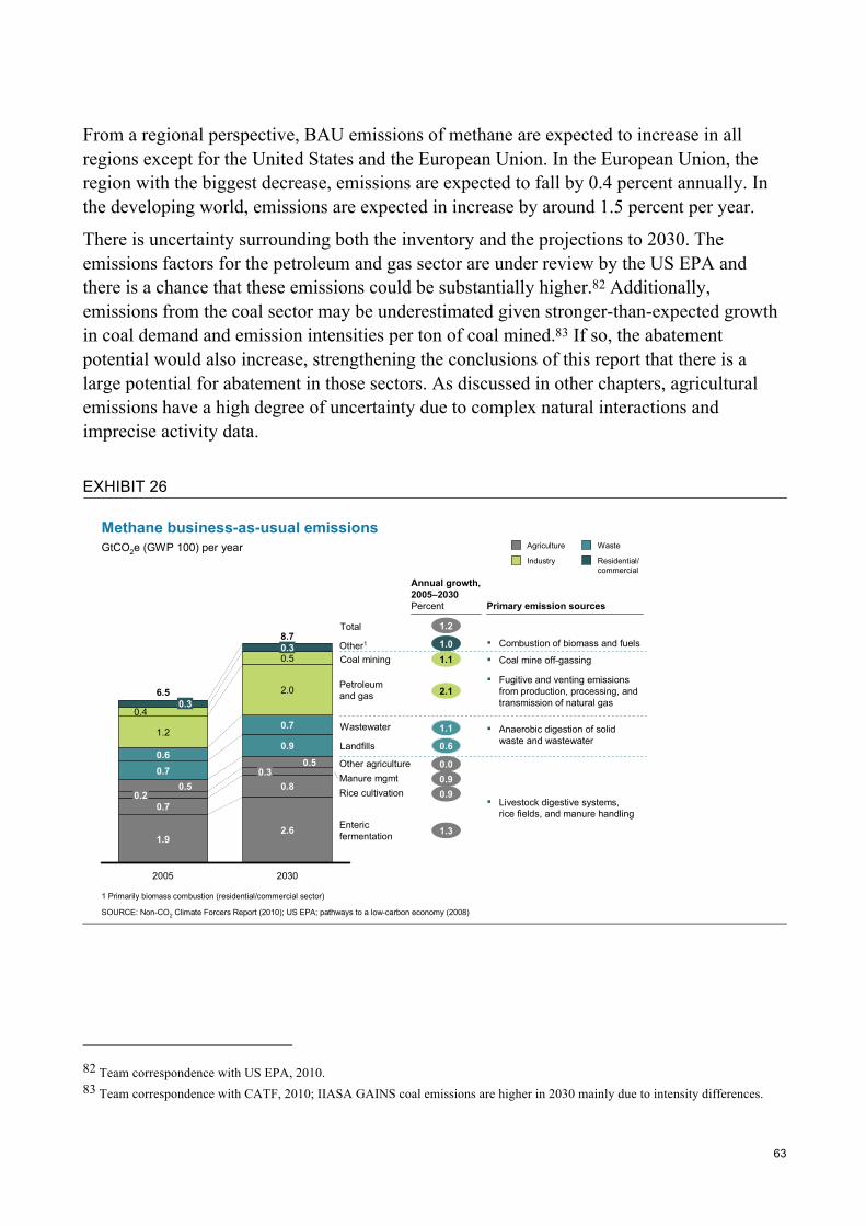
63

From a regional perspective, BAU emissions of methane are expected to increase in all regions except for the United States and the European Union. In the European Union, the region with the biggest decrease, emissions are expected to fall by 0.4 percent annually. In the developing world, emissions are expected in increase by around 1.5 percent per year.

There is uncertainty surrounding both the inventory and the projections to 2030. The emissions factors for the petroleum and gas sector are under review by the US EPA and there is a chance that these emissions could be substantially higher.82 Additionally, emissions from the coal sector may be underestimated given stronger-than-expected growth in coal demand and emission intensities per ton of coal mined.83 If so, the abatement potential would also increase, strengthening the conclusions of this report that there is a large potential for abatement in those sectors. As discussed in other chapters, agricultural emissions have a high degree of uncertainty due to complex natural interactions and imprecise activity data.

EXHIBIT 26

Landfills

Methane business-as-usual emissions

0.6

2.1

1.0

Entericfermentation

Rice cultivationManure mgmtOther agriculture

Petroleumand gas

Other1

0.7

0.8

0.50.9

0.50.3

2005

6.5

1.9

0.70.2

0.3

2.0

0.5

2030

8.7

2.6

0.7

0.30.4

0.6

1.2 1.1

0.00.90.9

1.3

Wastewater

Total 1.2

▪ Combustion of biomass and fuels


▪ Coal mine off-gassing

▪ Anaerobic digestion of solid waste and wastewater

▪ Livestock digestive systems, rice fields, and manure handling

▪ Fugitive and venting emissions from production, processing, and transmission of natural gas


Coal mining 1.1

1 Primarily biomass combustion (residential/commercial sector)

GtCO2e (GWP 100) per year Waste


Agriculture

Industry

SOURCE: Non-CO2 Climate Forcers Report (2010); US EPA; pathways to a low-carbon economy (2008)

82 Team correspondence with US EPA, 2010. 83 Team correspondence with CATF, 2010; IIASA GAINS coal emissions are higher in 2030 mainly due to intensity differences.

64

Abatement Potential Efforts to reduce methane emissions focus on capturing the gas where it is released into the atmosphere (Exhibit 27). There is abatement potential of 2.3 GtCO2e, representing a reduction of 26 percent from BAU levels.

EXHIBIT 27

Methane abatement cost curve – 2030

20

2.5

-80

140

120

0

-60

-20

-40Abatement potential

GtCO2e per year

180

1.00 1.5 2.00.5

160

Abatement cost, societal perspectiveUSD/tCO2e200

40

P&G midstream – distribution maintenance

P&G upstream – equipment upgrades

Landfill gas – direct useCoal mines – degasification and gas capture

P&G midstream – seals replacement

Coal mines – oxidation of ventilation air methaneRice cultivation – water management

Landfill gas – electricity generationManure management – covered anaerobic digester

P&G upstream – new operational practices

Livestock – antimethanogen vaccine

Livestock – feed supplements

Manure management –complete mix digester

Industrial wastewater –improved treatment

WasteAgriculture

Industry


P&G midstream – compressor maintenance



100-year GWP

Capturing the gas at landfills: Landfills generate methane when organic matter is decomposed by microorganisms under anaerobic conditions. Rather than allowing the gas to seep into the atmosphere, the gas can be captured and used to generate heat or electricity. There is also an opportunity to compost more of the new waste produced, and thereby lower emissions. In total, some 600 MtCO2e, or about 70 percent of emissions from landfills, can be captured. These are low-cost abatement measures, yielding an average societal profit of about $5/tCO2e. They also reduce the need for other sources of heat and power, but these secondary benefits are unquantified.

Natural gas and petroleum production: Methane is the largest component of natural gas, which is released (vented) at various stages of the gas production and transmission system. This is primarily a result of operational practices or equipment design—for example, compressors or pneumatic devices vent gas in order to control pressures, temperatures, or gas flows. In addition, natural gas accidentally leaks from the system, though this is a smaller component of the emissions. Methane emissions also occur to a smaller extent

65

during oil production at remotely located facilities where it is cheaper to vent excess natural gas than to transport it to distant consumers. By changing equipment and maintenance routines in both sub-sectors, emissions could be reduced by around 550 MtCO2e in 2030, representing more than 25 percent of total emissions, and at a societal profit of ~$5/tCO2e.

Collecting methane from coal mines: In the coal industry, most methane is released when underground coal mines are de-gassed prior to and during extraction, and when ventilation air is pumped from outside through the mines, picking up methane before being re-emitted to the atmosphere. Both practices take place in order to prevent explosions and so protect workers. Emissions can be reduced by capturing the methane released in the degasification process, and by the catalytic conversion of the ventilation air. The abatement potential in 2030 is about 200 MtCO2e, or 40 percent of BAU emissions, at a societal profit of ~$15/tCO2e.

Industrial wastewater treatment: All types of wastewater with organic components create methane. The methane emissions are most concentrated in industrial wastewater, especially the water from pulp and paper processing and food processing facilities. Systems that capture this methane can be installed in individual factories, yielding abatement potential of 150 MtCO2e at an average cost of about $180/tCO2e. However, this figure can vary widely due to different levels of concentration and, therefore, of the volumes of wastewater to be managed for a given amount of abatement. Methane is also produced in domestic wastewater. However, domestic wastewater is only likely to be collected and treated primarily to improve water quality and local health, as the costs are high. Methane reductions would be a side benefit.

Less concentrated amounts of methane are generated in the agricultural sector:

Rice cultivation water management: Methane is generated when rice paddy fields are flooded and organic matter is broken down by microorganisms under anaerobic conditions. Different watering methods, such as mid-season drainage and shallow flooding, would reduce emissions by 240 MtCO2e, or about 30 percent of rice methane emissions. These methods also reduce the amount of water needed for farming, which would increase the amount available for domestic use. The average societal profit of implementing these practices is around $2/tCO2e.84

Enteric fermentation: These emissions are a result of digestion in cattle and other ruminants. Potential abatement measures include dietary additives and vaccines, which together could cut emissions by around 500 MtCO2e in 2030. This is high in absolute terms, but represents only 20 percent of BAU levels. The average societal cost of these abatement measures is ~$25/tCO2e. Methane-reducing dietary additives and vaccines are a relatively recent technology, thus not fully field-proven. However, their abatement potential is 84 This cost would be partly offset by lower water usage (not quantified).

66

relatively certain. Further scientific research is ongoing that could uncover additional and improved methane abatement measures for livestock.

On top of technical abatement measures, it is worth mentioning the high potential that could be realized by reducing consumption of meat and dairy products. Reduced demand for these products would mean fewer animals, and hence fewer emissions. Earlier estimates put the abatement potential for reduced meat and dairy consumption at 1.8 GtCO2e,85 which, if included, would be the single largest emissions abatement opportunity.

Abatement benefits Methane is a precursor to tropospheric ozone, an air pollutant that impairs human health and vegetation growth.86 Reducing methane emissions would therefore improve public health and increase crop yields, as well as limit climate change.

Different studies link tropospheric ozone to cardiovascular and respiratory problems,87 which in turn contribute to morbidity. Some health studies have also identified a link between methane and mortality; the strength of the connection is under scientific debate.88 If the connection is as strong as West and Fiore 89 state, capturing the methane abatement potential identified in this report could prevent around 32,000 premature deaths in 2030. These figures should be regarded as an approximation, as the effects of the abatement identified in this study on methane concentrations are based on impact relations from scientific papers which have used climate and air quality models (see “Study Approach” chapter).90

A 2009 study91 examined the effect of ozone on four main crops, estimating the yield loss to be between 7 and 12 percent for wheat, 6 and 16 percent for soybean, 3 and 4 percent for rice, and 3 and 5 percent for maize. Measured in year 2000 prices, the corresponding global economic loss for these four crops was estimated at between $14 billion and $26 billion per year, about 40 percent of which was incurred by China and India.

In many parts of the world, domestic wastewater and human sewage are neither collected nor treated, spreading disease and taking a toll on human health.92 As mentioned earlier, 85 McKinsey & Company, 2009. 86 Royal Society, 2008. 87 See for example, Jerrett et al., 2010; Royal Society, 2008; Bell et al., 2004, Anenberg et al., 2009 for discussions on the health

impacts of tropospheric ozone. 88 The link between methane and mortality assumes that 1) methane contributes to all ozone concentrations and not just background


89 West et al., 2006; Fiore et al., 2008. 90 West et al., 2006; Fiore et al., 2008. 91 van Dingenen et al., 2009. 92 US EPA, 2006.

67

abatement measures on domestic wastewater were not covered in this analysis due to the high cost of water treatment from a pure methane abatement perspective. However, the WHO93 estimates that 1.8 million people die each year from diarrheal diseases, 90 percent of whom are children under five and who mostly live in developing countries. Around 88 percent of these cases of disease is attributable to insufficient water supply, poor sanitation, and poor hygiene. Wastewater treatment would help alleviate this health issue.

Implementation challenges The primary implementation challenges associated with methane abatement derive from the high number of emission sources, each of which will need to be tackled individually. In many developing countries, this is likely to require new institutional capacity. There is also a financing challenge, as discussed earlier in this report, as over 80 percent of methane emissions will occur in developing countries in 2030.

Abatement potential easier to capture in industry than agriculture: Capturing the abatement potential in the coal mining and petroleum and gas industry is relatively straightforward as the emissions are quite concentrated. There are also fewer decision-makers and stakeholders to address: it is much easier to reach 100 to 150 large public natural gas producers than it is to influence more than 2 million farmers in the US, for example.94

Food security must be maintained: For farmers to undertake new practices, such as reduced flooding or the use of feed supplements, there must be confidence that these practices will not reduce yields. Strong incentives, like through guarantees that compensate for the risk of financial losses, may be required to provide the farmer financial assurance.

Financing: While many abatement levers come at net savings from a societal perspective, from a project implementation perspective there will still be financing challenges – otherwise this abatement would be expected in the business-as-usual case. Financing solutions could include means to raise the investment returns over company hurdle rates or to force companies to realign internal resource allocation. Some levers, such as the livestock measures, have quite substantial abatement cost in some regions. Thus a purely emission reduction motivated cost coverage will need to be found – otherwise this potential will remain untapped.

93 WHO, 2005. 94 IHS Herold, 2010; US Department of Agriculture, 2009.

68

Nitrous oxide

Emission sources As with many other climate forcers, emissions of nitrous oxide occur both naturally and as a result of human activity. The largest human-induced emissions are a result of the use of nitrogen-based fertilizers. The increased abundance of soil nitrogen is then converted into nitrous oxide through various chemical processes in the nitrogen cycle – a natural process. Nitrous oxide also comes from wastewater and manure management, from the industrial production of nitric and adipic acid, and, to a smaller extent, from various kinds of fuel combustion.

Business-as-usual growth

In 2005, nitrous oxide emissions accounted for about 20 percent of non-CO2 emissions from human activities. Of the total 3.3 GtCO2e, the agricultural sector contributed about 2.8 GtCO2e, or about 85 percent. Total nitrous oxide emissions are expected to grow to 4.7 GtCO2e in 2030 under BAU conditions. This corresponds to annual growth of 1.5 percent, largely the result of population growth and hence more extensive use of fertilizers.95 (Exhibit 28).

The regional differences are large and, as in the case of methane, it is primarily the developing world that contributes to growth. Emissions in the fastest growing region, Latin America, are expected to grow by 2.3 percent annually. Emissions in the EU and the US are anticipated to remain more stable.

It should be noted that it is particularly difficult to estimate nitrous oxide emissions because a large percentage derives from natural processes. A number of site-specific conditions, such as temperature, add complexity in estimating the inventory and abatement potentials.

95 The 2005 inventory and the projections to 2020 are based on the US EPA’s 2006 Global Anthropogenic Emissions Report for all

sectors except for the chemicals sector (see Appendix F for assumptions). 2030 emissions are derived by applying the growth rates from 2015-2020 to the 2020 baseline.

69

EXHIBIT 28

Nitrous oxide business-as-usual emissions

0.0

0.1

2030

4.7

0.30.4

0.20.1

2005

3.3

3.5

0.3

2.3

0.20.3

0.20.1

Agricultural soils

Manure mgmtOther agricultureOther1

Acid production

1.7

1.2

▪ Chemical factories▪ Combustion of fuels

▪ Soil emissions as result of various human activities, e.g., fertilizer application

▪ Human sewage



TotalWastewater

1.60.90.81.5

1 Primarily byproduct of combustion (transport sector)

GtCO2e (GWP 100) per yearWaste

Transport

Agriculture

Industry

SOURCE: Non-CO2 Climate Forcers Report (2010); US EPA; pathways to a low-carbon economy (2008)

Abatement Potential There is a limited number of ways to reduce nitrous oxide emissions since most occur from fertilizer use in the agricultural sector. These emissions are particularly difficult to abate due to their linkage to food supply, but several mitigation measures have been identified. There is an abatement potential of 0.4 GtCO2e in 2030, representing almost 10 percent of total emissions (Exhibit 29). The potential lies in two key areas:

Agricultural soils: Nitrous oxide occurs naturally in soil because of microbial processes that are part of the nitrogen cycle. The application of fertilizer increases the nitrogen content and therefore nitrous oxide emissions. Better agricultural nutrient management and agronomy practices would reduce the amount of nitrogen that is needed for soil amendments. Examples include improved crop rotation, adjusted fertilizer application frequency, or using slow-release fertilizers. The abatement potential from these practices in 2030 is about 220 MtCO2e, or 6 percent of the soil emissions, and would have an average societal profit of over $5/tCO2e. Similar to the livestock levers, these improved practices are relatively recent and have not been rolled out on a larger scale to date; still, the potential to provide emissions reductions is relatively certain. Additional field research is needed to determine if any greater abatement potential from soils could be captured without

70

jeopardizing food production, decreasing soil carbon, or causing unintended land use change effects.

Acid production: Adipic acid and nitric acid are used for a variety of purposes, including the production of nylon and fertilizers. Nitrous oxide is formed as a byproduct and is typically released into the atmosphere. The installation of end-of-pipe controls to decompose the nitrous oxide would reduce emissions from acid production by around 150 MtCO2e, or 80 percent in 2030, for a societal cost of around $10/tCO2e.

EXHIBIT 29

0.4


-20

20

0

-40

Abatement potential GtCO2e per year

0.2

-60

0

60

40 Nitric acid production (retrofits) –gas decomposition

Croplands – improved agronomy practices

Nitric acid production (new) – gas decomposition

Rice cultivation – changed nutrient management

Grasslands – changed nutrient managementCroplands – changed nutrient management

Adipic acid production (new) – gas decompositionAdipic acid production (retrofits) – gas decomposition

Agriculture

Industry


Nitrous oxide abatement cost curve – 2030


100-year GWP

Abatement benefits Reducing nitrous oxide emissions will deliver additional, non-climate-related benefits, namely less water contamination from fertilizer and human sewage, and hence less environmental damage and better public health.

When fertilizer is washed from the soil, the nutrients leak into nearby water bodies, contaminating them. The biota of water bodies is held in equilibrium by a limited access to nutrients. The addition of nutrients can cause eutrophication in inland and coastal waters, which means encouraging the over-growth of algae, thus damaging fish and other water-

71

life.96 It also contaminates groundwater, threatening water supplies, as the effect is hard to reverse.97 Mineral fertilizers are the main culprits, but contamination is also linked to the use of manure.98 Changing both mineral fertilizer and manure practices would therefore improve water quality, save aquatic species, and reduce nitrous oxide emissions.

As discussed in the section on methane, domestic wastewater and human sewage are neither collected nor treated in many parts of the world, posing a significant risk to human health. Improving domestic wastewater treatment is expensive, however, and is not likely to be undertaken purely for its impact on climate change, so it is not included in the cost curve. However, its impact on health would be significant.

Implementation challenges Since nitrous oxide and methane share many of the same emission sources, they also share some of the implementation challenges. By 2030, about 75 percent of nitrous oxide emissions will be generated in developing countries, presenting the financing challenges discussed previously.

In the agricultural sector, farmers in both the developing and developed world will need to change the way they work if the potential abatement is to be realized. Institutional capacity will be required on a large scale to build awareness and capabilities.

For implementation to be successful, crop yields must be maintained – both to ensure food security and to maintain financial stability for farmers. There is also recent evidence that increased crop yields are beneficial for protecting forests.99 If yields were lower, more forests would be converted to croplands to support expanding populations, with a resulting decrease in carbon sequestration.

In addition, some form of guarantees or insurance policies against financial losses will likely be needed in order for farmers to voluntarily switch fertilizers or fertilize less. As it is difficult to measure agricultural nitrous oxide emissions, monitoring and compensating farmers for the changes that they undertake will pose an additional challenge.

96 FAO, 1996; Carpenter et al., 1998; Townsend et al., 2003. 97 Townsend et al., 2003. 98 FAO, 1996. 99 Burney, et al., 2010.

72

F-Gases

Emissions sources Fluorinated gases (f-gases) are increasingly being used as replacements for the ozone-depleting substances phased out by the Montreal Protocol. F-gases are used directly in some industrial processes and are produced as unwanted byproducts in the manufacturing of other materials:

■ Refrigerant: HFCs are coolant mediums used as replacements of ozone-depleting substances in refrigeration and air conditioning (e.g., pure HFC-134a or different blends of HFCs such as R-410A and R-404A).

■ Industry - Propellant: HFCs are used as propellants in, for example, metered dose inhalers for asthma and foam production (mainly HFC-134a and HFC-152a).

■ Industry - Dielectric medium: SF6 is used as an insulator in electric power transmission and distribution, as well as to protect magnesium from oxidation during production.

■ Byproduct: F-gas emissions also occur as unwanted byproducts in industrial production, e.g., HFC-23 (from HCFC-22 production) and aluminum (emissions of CF4 and C2F6).

It is worth mentioning that the F-gases are an environmental advancement over the ozone-depleting substances (ODSs), which they replace. The ODSs were found to deplete the ozone layer and many were also strong global warmers, whereas the f-gases have an impact on global warming only.

Business-as-usual growth F-gases are the smallest category of non-CO2 emissions that we have evaluated in this study, at approximately 0.5 GtCO2e in 2005 and growing to 1.6 GtCO2e in 2030.100 (Exhibit 30). Although small in 2005, f-gas emissions grow very quickly at ~5 percent per year. This growth is mainly due to the phase-out of ozone-depleting substances, which causes the HFCs that replace them to grow at ~7 percent annually and become the dominant source of f-gas emissions. This high growth in emissions is also expected to be maintained for decades thereafter, with some projections indicating f-gases as a very important source of all GHG emissions in 2050. In 2005 emissions came mainly from industrial sources and the ODS substitutes were less important. The main contributor to the emissions in 2030 is refrigeration and air conditioning with some 75 percent share.

100 We base both our 2005 inventory and the projections to 2020 on the US EPA’s 2006 Global Anthropogenic Emissions Report for

all sectors. We then grow those 2020 numbers to 2030 using the growth rates from 2005-2020. (See Appendix G for a list of assumptions.)

73

In 2030 the developing world is expected to have caught up with the developed world in f-gas emissions and to have a higher annual growth rate. This is because the developing world will start its phase-out of ODSs later than the developed world, and because it takes time before the phase-out is reflected in emissions. In the developed world the US produces a large share of f-gas emissions, due to large usage of refrigeration and air conditioning. The PFC and SF6 emissions are not expected to grow much, globally, due to voluntary industry commitments to reduce these very potent and long-lived gases.

Growth projections through 2030 are somewhat uncertain due to difficulty in estimating ODS phase-out rates, and the technologies that will be selected as the ODSs are phased out. Technology selection is important since the GWPs of replacement substances differ widely and energy efficiency plays an important role in emissions intensity.

EXHIBIT 30

F-gases business-as-usual emissions


▪ SF6 from transmission and distribution equipment

Residentialbuildings

Commercialbuildings

Transport

ChemicalsPower

2030

1.59

0.20

0.66

2005

0.110.11

0.13

0.10

0.50

0.01

0.04

0.34

0.28

0.040.07

7.6

14.0

4.6

3.0

-3.2

1.8

4.7Total

SOURCE: Non-CO2 Climate Forcers Report (2010); US EPA; Growth rates from Velders et al. 2009 and Gschrey and Schwarz (2009) beyond 2020


▪ Motor vehicle air conditioning systems

▪ Transport refrigeration

▪ Refrigeration, mainly retail food▪ Building air conditioning systems▪ Blowing agents for foam products

used for insulation

▪ Refrigeration and air conditioning ▪ Blowing agents for foam products

used for insulation

▪ HFC-23 as unwantedby-product of HCFC-22

▪ Production or use of aluminum and semiconductors

GtCO2e (GWP 100) of HFCs, PFCs and SF6 per year

Industry

Transport


Other industry

While newly manufactured ozone-depleting substances – CFCs and HCFCs – are being phased out by the Montreal Protocol, existing banks of these gases (contained in older refrigerators and building foams) are not covered by that agreement. Some of these banks are very hard to access but a substantial portion can be reached and destroyed at a reasonable cost. We have not included an analysis of the capture and destruction of the ODS banks, as these opportunities would be largely gone by 2030, resulting in little abatement at

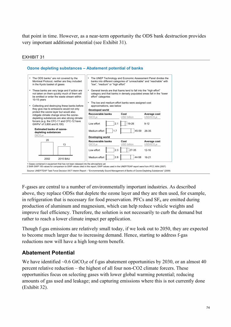
74

that point in time. However, as a near-term opportunity the ODS bank destruction provides very important additional potential (see Exhibit 31).

EXHIBIT 31

Ozone depleting substances – Abatement potential of banks

▪ The ODS banks1 are not covered by the Montreal Protocol, neither are they included in the Kyoto basket of gases

▪ These banks are very large and if action are not taken on them quickly much of them will be emitted or enter the waste stream within 10-15 years

▪ Collecting and destroying these banks before they give rise to emissions would not only protect the ozone layer but would also mitigate climate change since the ozone-depleting substances are also strong climate forcers (e.g. the CFC-11 and CFC-12 have GWPs2 of 3,800 and 8,100)

Source: UNEP/TEAP Task Force Decision XX/7 Interim Report – “Environmentally Sound Management of Banks of Ozone-Depleting Substances” (2009)

1 Gases contained in equipment that has not been released into the atmosphere yet2 SAR GWP 100 values for comparison to GWP values cited in this report, GWP values used in the UNEP/TEAP report were from IPCC AR4 (2007)

Recoverable banksGtCO2e

CostUSD billion

Developed world

9-12

Average costUSD/tCO2e

26-35

Recoverable banksGtCO2e

CostUSD billion

Developing world

12-16

Average costUSD/tCO2e

16-21

13

20

2015 BAU2002

Estimated banks of ozone-depleting substancesGtCO2e

▪ The UNEP Technology and Economic Assessment Panel divides the banks into different categories of “unreachable” and “reachable” with “low”, “medium” or “high effort”

▪ General trends are that foams tend to fall into the “high effort”category and that banks in densely populated areas fall in the “lower effort” categories

▪ The low and medium effort banks were assigned cost approximations, see below

19-26

45-59

2.1

1.7Medium effort

Low effort

27-35

44-58

2.3

2.8Medium effort

Low effort

F-gases are central to a number of environmentally important industries. As described above, they replace ODSs that deplete the ozone layer and they are then used, for example, in refrigeration that is necessary for food preservation. PFCs and SF6 are emitted during production of aluminum and magnesium, which can help reduce vehicle weights and improve fuel efficiency. Therefore, the solution is not necessarily to curb the demand but rather to reach a lower climate impact per application.

Though f-gas emissions are relatively small today, if we look out to 2050, they are expected to become much larger due to increasing demand. Hence, starting to address f-gas reductions now will have a high long-term benefit.

Abatement Potential We have identified ~0.6 GtCO2e of f-gas abatement opportunities by 2030, or an almost 40 percent relative reduction – the highest of all four non-CO2 climate forcers. These opportunities focus on selecting gases with lower global warming potential; reducing amounts of gas used and leakage; and capturing emissions where this is not currently done (Exhibit 32).

75

Refrigeration and air conditioning: The main abatement potential is in replacing high GWP gases with lower GWP gases. This can be accomplished in two major ways: changing the system to run on a new gas, or using a secondary loop that will bring down leakage and refrigerant charge size. Examples of alternative substances that can be used are ammonia and CO2 (when kept separate) or HFCs with lower GWP values, such as HFC-152a or HFC-1234yf. In motor vehicle air conditioning, the replacement with low-GWP technology is fairly close to commercialization; in retail food refrigeration it is already there. In other sectors where low-GWP solutions are not yet available, the abatement opportunity would be to decrease emissions by reducing leaks and/or recovering gas at disposal. Reducing leakage of these gases saves the cost of the refrigerants, which is fairly high. The combination of a high f-gas price, high GWP, and high share of labor costs makes these actions especially cost-efficient in the developing world. The identified abatement potential in refrigeration and air conditioning is ~550 MtCO2e, or 50 percent of the baseline, at about zero cost to society.

Increased leak repair and recovery in electric power: SF6 is used as an insulating gas in high-voltage equipment across the world and the gas is emitted through leakage during operation and equipment servicing. These emissions can be reduced at a fairly low cost, even negative cost for the first part of reductions as cost for insulating gas is saved. The identified abatement potential in electric power systems is ~40 MtCO2e, or 60 percent of the baseline at $3/tCO2e societal cost.

Thermal oxidation in industry: The HFC-23 that is produced as an unwanted byproduct in the production of HCFC-22 can be abated by thermal oxidation where it is collected and destroyed. The process of collecting and destroying the HFC-23 is very efficient but there is some downtime needed in the equipment, bringing down reduction efficiency to ~90 percent. Plants also need to be equipped with wastewater treatment capacity to handle the waste emissions resulting from the process. The identified abatement potential in HCFC-22 production is ~24 MtCO2e, or 54 percent of the baseline, at $4/tCO2e societal cost.

Foam alternatives (additional unquantified potential): The foams sector does not show big HFC emissions in the shorter term but the emissions occur slowly and large banks will be built up which will gradually emit the gases for extended periods of time. Today foams contain large banks of ozone-depleting substances that are hard to collect and destroy; in future decades the same problem can arise with HFCs. Additionally, foams can be produced using low-GWP gases or technologies not requiring HFC propellants. In designing abatement technologies for the foams sector it is important to maintain or improve energy efficiency, as any increased energy consumption could offset all the climate benefits of the reduced f-gas emissions. We estimate potential in this area could be ~30 MtCO2e but it is not included in the cost curve.

76

PFC and HFC emissions from industry (additional unquantified potential): A number of technical measures can also abate PFC and HFC emissions from industry. Abatement efforts are assumed already in the BAU baseline,101 yielding small remaining abatement potentials. We estimate these small but numerous opportunities could add up to ~90 MtCO2e but they are not included in the cost curve.

EXHIBIT 32

F-gases abatement cost curve – 2030

-8

0.30.2

Abatement cost, societal perspectiveUSD/t CO2e8

0.60.4

-4

0.7

4

0


0.50 0.1

Motor vehicle air conditioning systems – low-GWP refrigerants

HCFC-22 production –thermal oxidation of HFC-23


Residential/commercialIndustry

Transport

Large refrigeration systems – leak repair

Retail food refrigeration –distributed systems

Retail food refrigeration –secondary loop systems

Stationary air conditioning –refrigerant recovery

Electrical equipment –SF6 leakage reduction/ recovery

100-year GWP

Implementation challenges Compared to the other three non-CO2 climate forcers, the implementation challenges for f-gases are substantially smaller, especially because there are fewer decision makers to address.

Few manufacturers: There are a relatively limited number of manufacturers that produce f-gases, and so there are few decision makers who will need to change practices (e.g., car makers, HCFC-22 producers) and fewer monitoring resources will be required.

Capturing in-use emissions is harder: Where emissions are less linked to central manufacturers, they will be harder to control. For example, in leak repair or recycling of f-gas applications, many contractors will need to be educated on capturing these gases, and

101 The “Technology-adoption scenarios” from the US EPA’s 2006 Global Anthropogenic Emissions are used.

77

institutional capacity required to ensure compliance with recycling and destruction. This could be the largest implementation challenge in the f-gases, although experience has shown that the efforts are often easily accepted by contractors once they realize that for much of the abatement they can save money through reduced f-gas losses.

Financing: Capital constraints are not a significant barrier in the developed world, but could be important in the developing world. For example, more climate-friendly air conditioning for cars requires an extra initial investment, which will need to be borne by consumers.

78

References Arctic Council. Tromsø Declaration, 29 April 2009. Amann, M. et al. GAINS Asia, “Scenarios for cost-effective control of air pollution and greenhouse gases in China.” 2008a. Amann, M. et al. 2008b. GAINS-ASIA, “A tool to combat air pollution and climate change simultaneously.” Methodology report. International Institute for Applied Systems Analysis (IIASA), Laxenburg, Austria, 2008b. Anenberg, S.C., et al. “An estimate of the global burden of anthropogenic ozone and fine particulate matter on premature human mortality using atmospheric modeling.” Environmental Health Perspectives (2010). BBC, “Third of China hit by acid rain,” citing the Chinese Bureau of Statistics, 27 August 2006. http://news.bbc.co.uk/2/hi/asia-pacific/5290236.stm

Bell, M.L. et al. “Ozone and short-term mortality in 95 US urban communities, 1987-2000.” Journal of the American Medical Association 292, no. 19 (2004). Berntsen, T., Tanaka, K., and Fuglestvedt, J.S. “Does black carbon abatement hamper CO2 abatement?” Climatic Change 103 (2010). Bice, K., A. et al. Black Carbon: A Review and Policy Recommendations. Woodrow Wilson School of Public & International Affairs: Princeton University, 2009. Biswas, D.K. and Pandley, G.K. “Strategy and Policy adopted in Air Quality Management in India Better Air Quality in Asian and Pacific Rim Cities (BAQ 2002).” Hong Kong SAR, 16– 18 Dec, 2002. Blowers, P. and Lownsbury, J.M. “Carbon dioxide emission implications if hydrofluorocarbons are regulated: a refrigeration case study.” Environmental Science & Technology 44, no. 5 (2010). Bond, T. C. et al. “A technology-based global inventory of black and organic carbon emissions from combustion.” Journal of Geophysical Research 109 (2004). Bond, T. C. and Sun, H. Can reducing black carbon emissions counteract global warming?” Environmental Science & Technology 39, no. 16 (2005). Bond, T. C. “Can warming particles enter global climate discussions?” Environmental Research Letters 2 (2007). Bond, T. C. et al. “Historical emissions of black and organic carbon aerosol from energy-related combustion.” Global Biogeochemical Cycles 21 (2007): 1850–2000. Boucher, O. and Reddy, M.S. “Climate trade-off between black carbon and carbon dioxide emissions.” Energy Policy 1, no. 6 (2008): 193-200. Burney, J.A. et al. “Greenhouse gas mitigation by agricultural intensification.” Proceedings of the National Academy of Sciences, Early Edition (2010). California Environmental Protection Agency. California Facilities and Greenhouse Gas Emissions Inventory – High-Global Warming Potential Stationary Source Refrigerant Management Program. Appendix B of the California Global Warming Solutions Act of 2006, 2009. California Environmental Protection Agency. Economic Impact Estimates – High-Global Warming Potential Stationary Source Refrigerant Management Program. Appendix C of the California Global Warming Solutions Act of 2006, 2009.

79

Carmichael, G.R. et al. “Asian aerosols: Current and year 2030 distributions and implications to human health and regional climate change.” Environmental Science & Technology 43. no.15 (2009). Carpenter et al. “Nonpoint pollution of surface waters with phosphorus and nitrogen.” Ecological Applications 8, no. 3 (1998). China Daily. “Beijing narrowly attains 'blue sky' goal,” Jan. 1, 2008. Data used in the passage is from Beijing Bureau of Environmental Protection. http://www.chinadaily.com.cn/china/2008-01/01/content_6362366.htm. ChinaFAQs. “ChinaFAQs: China’s Carbon Intensity Goal: A Guide for the Perplexed.” World Resources Institute, 12 April 2009. http://tiny.cc/iojmt Cofala, J. et al. “Scenarios of global anthropogenic emissions of air pollutants and methane until 2030.” Atmospheric Environment 41 (2007): 8486-8499. Cohen, A.J. et al. “The global burden of disease due to outdoor air pollution.” Journal of Toxicology and Environmental Health, Part A, no. 68 (2005). Daniel, J.S., Solomon, S., and McFarland, M. “A Limitation of Global Warming Potentials Revisited.” in IPCC Final Report of the Expert Meeting on the Science of Alternative Metrics, March 18-20, 2009. de Cara, S., Houze, M., and P-A Jayet. “Methane and nitrous oxide emissions from agriculture in the EU: a spatial assessment of sources and abatement costs.” Environmental & Resource Economics 32 (2005): 551–583. den Elzen, M. and Meinshausen, M. Multi-Gas Emission Pathways for Meeting the EU 2°C Climate Target: global and regional emission implications. Netherlands Environmental Assessment Agency, 2006. http://tinyurl.com/489ezr den Elzen, M; Meinshausen, M; van Vuuren, D. “Multi-gas emission envelopes to meet greenhouse gas concentration targets: Costs versus certainty of limiting temperature increase.” Global Environmental Change, 2007. http://tinyurl.com/9bpnnt den Elzen, MGJ. and van Vuuren, DP. “Peaking profiles for achieving long-term temperature targets with more likelihood at lower costs.” Proceedings of the National Academy of Sciences (2007). European Commission. Adapting to climate change: towards a European framework for action. White Paper, 2009. European Union (EU). 20-20-20 Targets, 2007, http://ec.europa.eu/environment/climat/climate_action.htm European Union (EU). EU Mobile Air Conditioning Directive, 2006. http://tiny.cc/57phw Eurostat. Population data, 2009. Ezzati, M. et al. “Comparative quantification of mortality and burden of disease attributable to selected risk factors.” In: Global Burden of Disease and Risk Factors, ed. by Alan D. Lopez, Colin D. Mathers, Majid Ezzati, Dean T. Jamison, and Christopher JL Murray. Washington: World Bank, 2006. Federal Environment Agency – Germany. Natural refrigerants – CO2-based air conditioning system put to practical testing. Research project under the Environmental Research Plan of the Federal Ministry for the Environment, 2009. Federal Environment Agency – Germany, Projections of global emissions of fluorinated greenhouse gases in 2050. Research project under the Environmental Research Plan of the Federal Ministry for the Environment, 2009. (http://tinyurl.com/37ahm4l)

80

Finnveden, Göran et al. “Flexible and robust strategies for waste management in Sweden.” Waste Management 27 (2007): S1–S8. Fiore, A.M. et al. “Characterizing the tropospheric ozone response to methane emission controls and the benefits to climate and air quality.” Journal of Geophysical Research 113 (2008). Food and Agricultural Policy Research Institute (FAPRI). U.S. and World Agricultural Outlook. FAPRI Staff Report 07-FSR 1, 2007. Food and Agriculture Organization (FAO) of the United Nations. Control of Water Pollution from Agriculture. FAO Irrigation and Drainage Paper – 55, 1996. Food and Agriculture Organization of the United Nations (FAO). Fertilizer requirements in 2015 and 2030, 2000. Fuglestvedt, J.S., et al. “Transport impacts on atmosphere and climate: Metrics.” Atmospheric Environment 2009. doi:10.1016/j.atmosenv.2009.04.044 Guardian, “Satellite data reveals Beijing as air pollution capital of world,” citing the Chinese Academy on Environmental Planning report, 31 October 2005. http://www.guardian.co.uk/news/2005/oct/31/china.pollution Habets, L. et al. “The value of anaerobic purification for pulp and paper mill effluents.” TAPPI Environmental. 2002. Harnisch, J. et al. Abatement of other greenhouse gases - Engineered chemicals. Internal report - IEA Greenhouse Gas R&D programme, 2001. Harnisch, J. and Gluckman, R. Final Report on the European Climate Change Programme, Working Group – Industry, Work Item - Fluorinated Gases. Prepared on behalf of the European Commission, 2001. Harnisch, J. and Hendriks, C. Economic Evaluation of Emission Reductions of HFCs, PFCs and SF6 in Europe, Prepared on behalf of the Commission of the European Union – Directorate General Environment, 2000. Heierli, U, and Maithel, S. Brick by brick: the Herculean task of cleaning up the Asian brick industry. Swiss Agency for Development and Cooperation (SDC), Natural Resources and Environment Division, Berne, 2008. ICF International. Regulatory Impact Analysis – The Substitutes Recycling Rule. Report prepared for US EPA, 1998. IHS Herold, Financial & Operating Database, 2010. IIPS, National Family Health Survey (NFHS-3), 2005–06. Mumbai: International Institute for Population Sciences, 2007. Immerzeel, W.W. et al. “Climate Change Will Affect the Asian Water Towers.” Science 328 (2010): 1382. Intergovernmental Panel on Climate Change (IPCC). Second Assessment Report (AR2), 1995. Intergovernmental Panel on Climate Change (IPCC). Technologies, Policies and Measures for Mitigating Climate Change, IPCC Technical Paper – 1 – Solid Waste and Wastewater Disposal, 1996. http://tinyurl.com/258skyk Intergovernmental Panel on Climate Change (IPCC). Climate Change 1995: The Science of Climate Change. Contribution of Working Group I to the Second Assessment Report of the Intergovernmental Panel on Climate Change. Houghton, J.T. et al. (eds.), Cambridge University Press, 1996. Intergovernmental Panel on Climate Change (IPCC) / Technology and Economic Assessment Panel (TEAP) of the Montreal Protocol, Safeguarding the Ozone Layer and the Global Climate System: Issues Related to Hydrofluorocarbons and Perfluorocarbons. IPCC/TEAP Special Report, 2005.

81

Intergovernmental Panel on Climate Change (IPCC). 2006 IPCC Guidelines for National Greenhouse Gas Inventories, 2006. Intergovernmental Panel on Climate Change (IPCC). Fourth Assessment Report (AR4), 2007. International Energy Agency (IEA). World Energy Outlook 2006. International Energy Agency (IEA). World Energy Outlook 2007 (and associated back-up data directly from IEA). International Energy Agency (IEA). World Energy Outlook 2009 (and associated back-up data directly from IEA). International Food Policy Research Institute (IFPRI). Agricultural Resources by Country by Year, 2010. International Institute for Applied Systems Analysis (IIASA), GAINS model, accessed February – July 2010. Jerrett, et al. “Long-term ozone exposure and mortality.” The New England Journal of Medicine 360 (2009):1085-1095. Kankaanpaa, Susanna and Carter, Timothy. Construction of European forest land use scenarios for the 21st century. The Finnish Environment Institute, 2004. http://tinyurl.com/95suoo Klimont, Z.; et al. Modelling Particulate Emissions in Europe - A Framework to Estimate Reduction Potential and Control Costs, International Institute for Applied Systems Analysis (IIASA) Interim Report IR-02-076, 2002. Kopp, RE, and Mauzerall, DL. “Assessing the climatic benefits of black carbon mitigation.” Proceedings of the National Academy of Sciences, Early Edition (2010): 11703-11708. Kroeger, T. Black Carbon Emissions in Asia: Sources, Impacts and Abatement Opportunities. Contractor report prepared for International Resources Group, LLC, 2010. Lamarque,J.-F. et al. “Historical (1850-2000) Gridded anthropogenic and biomass burning emissions of reactive gases and aerosols: methodology and application.” Atmospheric Chemistry and Physics Discussions 10 (2010): 4963-5019. Lenton, TM, et al. “Tipping elements in the Earth’s climate system.” Proceedings of the National Academy of Sciences 105, no. 6. (2008): 1786-1793. Living from Beijing. “Summary of Beijng’s 2009 Air Quality,” 31 December 2009, citing the China Environmental Protection Yearbook. http://tiny.cc/qp513 Lopez, A.D. et al. (eds.) Global Burden of Disease and Risk Factors, World Bank and Oxford University Press, 2006. McKinsey & Company. Pathways to a Low-Carbon Economy – Version 2 of the Global Greenhouse Gas Abatement Cost Curve, 2009. Meinshausen, M. “What does a 2°C target mean for greenhouse gas concentrations? – A brief analysis based on multi-gas emission pathways and several climate sensitivity uncertainty estimates.” Chapter 6 of Avoiding Dangerous Climate Change, Cambridge University Press, 2006. Methane to Markets. United States Profile of Solid Waste Disposal Practices and Strategic Plan for Landfill Gas Management. Methane to Markets Partnership Landfill Subcommittee, 2008. http://tinyurl.com/2ejnxus Miller, T.R, Variations between countries in value of statistical life, Journal of Transport Economics and Policy 34 Part 2 (2000): 169-188. Molina, M. et al. “Reducing abrupt climate change risk using the Montreal Protocol and other regulatory actions to complement cuts in CO2 emissions.” Proceedings of the National Academy of Sciences, Early Edition. 2009.

82

Monni, Suvi, et al. Global climate change mitigation scenarios for solid waste management. VTT Technical Research Centre of Finland, 2006. Moulton, R. J., and Richards, K.R. Costs of sequestering carbon through tree planting and forest management in the United States. United States Department of Agriculture, 1990. Netherlands Environmental Assessment Agency (MNP), and Organisation for Economic Co-Operation and Development (OECD), Background report to the OECD Environmental Outlook to 2030 Overviews, details, and methodology of model-based analysis, Report 500113001, 2008 Organization for Economic Co-Operation and Development (OECD). OECD Environmental Outlook to 2030, 2008. Pan et al. “Health benefit evaluation of the energy use scenarios in Beijing, China.” Science of the Total Environment 374 (2007). People’s Republic of China. Initial National Communication on Climate Change. Beijing, 2004. Pettus, A. Agricultural Fires and Arctic Climate Change, Report for the Clean Air Task Force, available at: http://www.catf.us/publications/view/99, 2009. Pew Center on Global Climate Change. Black Carbon – A Science / Policy Primer. 2009. Ramanathan, V. and Carmichael, G. “Global and regional climate changes due to black carbon.” Nature Geoscience, Vol. 1. (2008). Ramanathan, V. et al. Atmospheric Brown Clouds – Regional Assessment Report with Focus on Asia. United Nations Environment Programme (UNEP). 2008. Ramanathan, V and Xu Y. “The Copenhagen Accord for limiting global warming: Criteria, constraints, and available avenues.” Proceedings of the National Academy of Sciences 107, no. 18 (2010): 8055-8062. REN21. Renewables 2007 Global Status Report, available at: http://www.ren21.net/pdf/RE2007_Global_Status_Report.pdf, accessed June 2010. Republic of India, Ministry of Environment and Forests. India’s Initial National Communication to the United Nations Framework Convention on Climate Change. 2004. Republic of India. National Action Plan on Climate Change. Prime Ministers Council on Climate Change, 2008. Republic of India. Jawaharlal Nehru National Solar Mission. 2010. Root, TL et al. “Fingerprints of global warming on wild animals and plants.” Nature 421 (2003): 57-60. Rounsevell, M. et al. “A coherent set of future land use change scenarios for Europe.” Agriculture, Ecosystem and Environment. 2006. http://tinyurl.com/7ee4tk Royal Society. Ground-level ozone in the 21st century: future trends, impacts and policy implications. Royal Society Science Policy Report – 15/08. 2008. Ruckstuhl, C. et al. “Aerosol and cloud effects on solar brightening and the recent rapid warming.” Geophysical Research Letters 35 (2008): L12708. Rugh, J. et al. “Significant Fuel Savings and Emission Reductions by Improving Vehicle Air Conditioning.” 15th Annual Earth Technologies Forum and Mobile Air Conditioning Summit, National Renewable Energy Laboratory, 2004.

83

Rypdal, K. et al. “Costs and global impacts of black carbon abatement strategies.” Tellus Series B Chemical and Physical Meteorology 61B (2009): 625-641. SAE International. Industry Evaluation of low global warming potential refrigerant HFO-1234yf, 2009. http://tinyurl.com/32rt6kt Schaefer, D.O. et al. “Estimating Future Emissions and Potential Reductions of HFCs, PFCs, and SF6.” The Energy Journal, 2006. Schindell, D. et al. “Climate forcing and air quality change due to regional emissions reductions by economic sector.” Atmospheric Chemistry and Physics 8 (2008): 7101–7113. Scheehle, E.A. and Doorn, M.R.J. Improvements to the U.S. Wastewater Methane and Nitrous Oxide Emissions Estimates, 2003. http://tiny.cc/hhfzw Schellnhuber, Hans Joachim et al. Avoiding Dangerous Climate Change. Cambridge University Press, 2006 Smith, Alison; Brown, Keith; Ogilvie, Steve; Rushton, Kathryn; and Bates, Judith. Waste management options and climate change, Final report to the European Commission, DG Environment, 2001. Smith, K.R. “National burden of disease in India from indoor air pollution.” Proceedings of the National Academy of Sciences 97. no. 24 (2000). Smith, K.R.; et al. “Public health benefits of strategies to reduce greenhouse-gas emissions: health implications of short-lived greenhouse pollutants.” The Lancet (online), 2009. Smith, Pete et al. “Greenhouse gas mitigation in agriculture.” Philosophical Transactions of the Royal Society B 363 (2008): 789–813. http://www.eoearth.org/article/Greenhouse_gas_mitigation_in_agriculture Spokas, Kurt et al. “Developing a Field-Validated Methodology for a Regional GHG Inventory: Improved Methods for Landfill CH4 Emissions in California.” Presentation to Global Waste Management Symposium, Copper Mountain, CO, 2008. http://tinyurl.com/8gozmx SRI Consulting. CEH Marketing Research Report: Nitric Acid. Donald H. Lauriente, 2007. Streets, D.G., Wu, Y, and Chin, M. “Two–decadal aerosol trends as a likely explanation of the global dimming/brightening transition.” Geophysical Research Letters 33 (2006): L15806. Tohka, A. The GAINS Model for Greenhouse Gases – Version 1.0: HFC, PFC and SF6. International Institute for Applied Systems Analysis (IIASA) Interim Report IR-05-56, 2005. Townsend et al. “Human health effects of a changing global nitrogen cycle.” Frontiers in Ecology and the Environment 1, no. 5 (2003). United Nations Environment Programme (UNEP). Assessment of Alternatives To HCFCs And HFCs And Update Of The TEAP 2005 Supplement Report Data. Report of the UNEP Technology and Economic Assessment Panel, 2009. United Nations Environment Programme (UNEP). Environmentally Sound Management Of Banks Of Ozone-Depleting Substances. Report of the UNEP Technology and Economic Assessment Panel, 2009. United Nations Environment Programme (UNEP) Partnership for Clean Fuels and Vehicles, http://www.unep.org/transport/pcfv/, accessed June 2010. United Nations Framework Convention on Climate Change (UNFCCC). Copenhagen Accord. United Nations Climate Change Conference, Copenhagen, 2009.

84

United Nations Statistics Division. Environmental Indicators, Municipal Waste Composition data, last updated 2007. United States. Air Quality Management in the United States. Committee on Air Quality Management in the United States, Board on Environmental Studies and Toxicology, Board on Atmospheric Sciences and Climate, Division on Earth and Life Studies, National Academy of Sciences, 2004. United States, American Recovery and Reinvestment Act, 2009. United States Agency for International Development (USAID). Black Carbon Emissions in Asia – Sources, Impacts and Abatement Opportunities, 2010. United States Census Bureau, Population data, 2009. United States Department of Agriculture. Census of Agriculture Shows Growing Diversity in U.S. Farming. News Release, 2009. http://tinyurl.com/cakk5y United States Environmental Protection Agency. U.S. Methane Emissions 1990-2020: Inventories, Projections, and Opportunities for Reductions, 1999. United States Environmental Protection Agency. Assessment of the Worldwide Market Potential for Oxidizing Coal Mine Ventilation Air Methane, 2003. United States Environmental Protection Agency. Energy from Ventilation Air Methane (VAM) Using Oxidation Technologies, EPA Coalbed Methane Outreach Program Technical Options Series, 2004. United States Environmental Protection Agency. Managing Manure with Biogas Recovery Systems - Improved Performance at Competitive Costs, 2006. United States Environmental Protection Agency. Global Anthropogenic Non-CO2 Greenhouse Gas Emissions: 1990 – 2020, 2006. United States Environmental Protection Agency. Global Mitigation of Non-CO2 Greenhouse Gases, 2006 United States Environmental Protection Agency. Coal Mine Methane Recovery: A Primer, 2009 United States Environmental Protection Agency. “Endangerment and Cause or Contribute Findings for Greenhouse Gases Under Section 202(a) of the Clean Air Act; Final Rule,” 40 CFR Chapter I, 74 Federal Register 239 (15 December 2009): 66496 – 66546.

United States Environmental Protection Agency. “Light-Duty Vehicle Greenhouse Gas Emission Standards and Corporate Average Fuel Economy Standards; Final Rule,” 40 CFR Parts 85, 86, and 600; 49 CFR Parts 531, 533, 536, et al., 75 Federal Register 88 (7 May 2010): 25323-25728. United States Environmental Protection Agency. Inventory of U.S. Greenhouse Gas Emissions and Sinks: 1990 – 2008, 2010. United States Environmental Protection Agency. History of the Clean Air Act, http://www.epa.gov/air/caa/caa_history.html, accessed June 2010 van Dingenen, R. et al. “The global impact of ozone on agricultural crop yields under current and future air quality legislation.” Atmospheric Environment 43 (2009). van Vuuren, D., Weyant, J., and de la Chesnaye, F. “Multi-gas scenarios to stabilize radiative forcing.” Energy Economics 28 (2006): 102–120. Velders, G.J.M. et al. “The importance of the Montreal Protocol in protecting climate.” Proceedings of the National Academy of Sciences 104, no. 12 (2007).

85

Velders, G.J.M. et al. “The large contribution of projected HFC emissions to future climate forcing.” Proceedings of the National Academy of Sciences 106, no. 27 (2009). Wang, X. and Mauzerall, D.L. “Characterizing distributions of surface ozone and its impact on grain production in China, Japan and South Korea: 1990 and 2020.” Atmospheric Environment 38 (2004). Wang, X. and Mauzerall, D.L. “Evaluating impacts of air pollution in China on public health: Implications for future air pollution and energy policies.” Atmospheric Environment 40 (2006). West, J.J.; et al. “Global health benefits of mitigating ozone pollution with methane emission controls.” Proceedings of the National Academy of Sciences 103, no. 11 (2006). Wilson, Richard and Spengler, John, eds. Particles in Our Air: Concentrations and Health Effects, p 212, 1999. World Health Organisation (WHO). Water, Sanitation and Hygiene Links to Health - Facts and Figures, last updated in November 2004, 2005. World Health Organisation (WHO). Mortality Country Fact Sheet - India, 2006. World Health Organisation (WHO). The Global Burden of Disease – 2004 update, 2008. World Health Organisation (WHO). The Global Health Risks: mortality and burden of disease attributable to selected major risks, 2009. World Health Organisation (WHO). Progress on Sanitation and Drinking Water – 2010 Update, 2010. Xu, B.; et al. “Black soot and the survival of Tibetan glaciers.” Proceedings of the National Academy of Sciences, Early Edition (2009). Zhang, J.J. and Smith, K.R. “Household Air Pollution from Coal and Biomass Fuels in China: Measurements, Health Impacts, and Interventions.” Environmental Health Perspectives 115, no. 6 (2007). Zhang, J.J.; et al. “Environmental health in China: progress towards clean air and safe water.” The Lancet 375 (2010).

86

Appendix A: Key Contacts and Contributors

Key contacts For further information about this report, please contact Matt Lewis, Communications Director, ClimateWorks Foundation, email: [email protected].

Contributors We would like to gratefully thank all of the contributors, who truly enabled this report to come to fruition.

ClimateWorks Governing Board Members Hal Harvey President, ex officio board member Mario

Molina

Co-recipient of the 1995 Nobel Prize in chemistry and professor at the University of California, San Diego, with a joint appointment at the Scripps Institution of Oceanography

Betrand Collumb Honorary chairman of Lafarge, the worldwide leader in building materials with 90,000 employees in 80 countries

Steering Committee Members We would like to extend a special thank you to the members of our Steering Committee, who offered their time and expertise to ensure we were pointed in the right direction.

Marcus Amann International Institute for Applied Systems Analysis (IIASA) Armond Cohen Clean Air Task Force Andreas Merkl ClimateWorks Foundation Ding Yihui China Meteorological Administration

External contributors Stephen O. Andersen Montreal Protocol Technology and Economic Assessment Panel (TEAP) Ellen Baum Clean Air Task Force Tami Bond University of Illinois, Urbana-Champaign Gus Cerri Honeywell Joseph Chaisson Clean Air Task Force Yingjun Chen Yantai Institute of Coastal Zone Research, Chinese Academy of Sciences Xiaofu Chen China Association of Rural Energy Industry David Diggs Honeywell Roger Fernandez US EPA Mike Fowler Clean Air Task Force Axel Friedrich Umweltbundesamt (UBA), retired Glenn Gallagher California Air Resources Board (ARB) Michelle Garcia California Air Resources Board (ARB)

87

Kenneth Gayer Honeywell David S. Godwin US EPA Rachel Goldstein US EPA Mark W. Grobmyer SEAF Cleantech Deployment Fund Paul Gunning US EPA Pamela Gupta California Air Resources Board (ARB) Kebin He Tsinghua University Lena Höglund International Institute for Applied Systems Analysis (IIASA) Tao Huai California Air Resources Board (ARB) Kejun Jiang China Energy Resources Institute (ERI) Zbigniew Klimont International Institute for Applied Systems Analysis (IIASA) Michael Lawrence Honeywell Dave Mehl California Air Resources Board (ARB) Mark A. Miller Greenhouse Gas Services, LLC, A GE AES Venture Hu Min China Sustainable Energy Program Ray J. Minjares International Council on Clean Transportation (ICCT) Thomas Morris Honeywell Jeffrey Neumann Honeywell Sara Ohrel US EPA Raymond Pilcher Raven Ridge Resources Shaun Ragnauth US EPA Didier Rotsaert AES Elizabeth Scheehle California Air Resources Board (ARB) Pete Smith University of Aberdeen Kristen Taddonio US EPA Jimmy Tran University of California, Berkeley Joop van der Steen Shell Projects and Technology Michael P. Walsh International Council for Clean Transportation (ICCT) Jason J. West University of North Carolina Qiang Zhang Tsinghua University

Project team We would also like to thank the ClimateWorks project leadership, including Catherine Witherspoon, Jane Chao, and Jie Cheng. McKinsey & Company provided the analytical support for this report and we would like to thank the core members of their team: Jens Dinkel, Per-Anders Enkvist, Abhishek Goyal, Rahul K Gupta, Niclas Nylund, Alissa Jones Peterson, Sebastian Schienle, Abhishek Singh, and Anders Åhlén, along with all of their other colleagues that offered comments and support.

88

Appendix B: Glossary Abatement costs Additional costs (or net benefit) based on the use of a technology with low global

warming impact compared with the impact of the current business-as-usual technology projection. In this study, these are assessed from a societal perspective, i.e., taking into account a long-term bond rate for the interest rate and full lifetime for the amortization periods. Measured as USD per tCO2e abated emissions. Includes annualized CapEx repayments and OpEx

Abatement Compilation of abatement potentials and costs cost curve

Abatement lever See “lever”

Abatement potential Incremental technical potential for reducing emissions by implementing an abatement lever, only limited by technical constraints (e.g., maximum industry capacity build-up). Potential is incremental to business-as-usual

Aerosol Small solid particles in the atmosphere

Atmospheric lifetime A climate science term used to describe the rate at which climate forcers are removed from the atmosphere once emitted

Black Carbon Commonly known as a component of soot. It is an aerosol that is differentiated from co-emitted organic carbon because it is black in color and therefore absorbs light

Business-as-usual Baseline emissions scenario to which abatement potential refers. Based primarily on external forecasts, e.g., IEA and EPA projections. Also referred to as BAU in the report

CapEx Incremental capital expenditure (investment) required for an abatement lever compared with business-as-usual

Climate forcers The term used to describe emissions that change the equilibrium temperature of the earth. For the context of this report, it includes carbon dioxide, methane, black and organic carbon, f-gases and nitrous oxide

CO2 Carbon dioxide

CO2e Carbon dioxide equivalent is the unit for emissions that, for a given amount of climate forcer, represents the amount of CO2 that would have the same global warming potential (GWP) when measured over a specified timescale (generally, 100 years)

Decision maker The party that decides on making an investment, i.e., the company (e.g., as owner of an industrial facility) or the individual (e.g., as owner of a car or home)

F-gases Fluorinated gases. Refers to HFCs (hydrofluorocarbons), PFCs (perfluorocarbons) and SF6 (sulfur hexafluoride). These gases are all covered under the Kyoto Protocol. In this report, the term does not refer to the CFCs or HCFCs, which are covered under the Montreal Protocol.

Greenhouse gas Greenhouse gas in the context of the Kyoto Protocol, i.e., CO2 (GHG) (carbon dioxide), CH4 (methane), N2O (nitrous oxide), HFC/PFC (hydrofluorocarbons), and SF6 (sulfur hexafluoride)

Gt Gigatonne(s), i.e., one billion (109

) metric tonnes

89

GWP Global warming potential. an index based upon radiative properties that measures the radiative forcing of a unit mass in today’s atmosphere integrated over a chosen time horizon, relative to that of CO2. The GWP represents the combined effect of the differing lengths of time that these gases remain in the atmosphere and their relative effectiveness in absorbing radiation

HDV Heavy duty vehicle

Inventory Inventory is the estimation of emissions in the base year. The base year used in this analysis is generally 2005. The inventory is the historical emissions level from which projections to 2030 start out

kWh Kilowatt hour(s)

(Abatement) lever Technological approach to reducing greenhouse gas emissions, e.g., use of more efficient processes or materials

LDV Light duty vehicle

MDV Medium duty vehicle

Monte Carlo analysis A statistical computation method for analyzing systems with many interdependent variables. For each variable, a range of potential values is defined and assigned probabilities. A random value within the defined range for each variable is chosen and used in the calculation. This is repeated many times (over 1,000 for the analysis in this report) and the results are aggregated to get the expected value and range of outcomes

Mt Megatonne(s), i.e., one million (1,000,000) metric tonnes

MWh Megawatt hour(s), i.e., one million Watt hours

OpEx Incremental operating cost required for the abatement lever compared to business-as-usual. Includes incremental operational and maintenance cost and incremental savings (e.g., from reduced energy consumption)

Radiative forcing Change in the net energy at the top of the atmosphere (tropopause) due to a change such as the composition of the atmosphere or the net output of the Sun. The change in radiative forcing, along with other climate system properties, is used to estimate the change in global temperatures that is caused by human activities. Please refer to the IPCC Assessment Report 4 (AR4) for further discussion.

Sector Grouping of businesses or areas emitting climate forcers, specifically:

Industry: Direct emissions of all industrial branches with the exception of the transportation sector, and including the power sector Residential/Commercial: Direct emissions from private households and the tertiary sector (commercial, public buildings, buildings used in agriculture). Indirect emissions are accounted for in the power sector Transport: Emissions from road transport (passenger transportation, freight transportation), as well as sea and air transport Waste: Emissions from disposal and treatment of waste and sewage Agriculture and Forestry: Emissions from livestock farming and soil

90

management. Emissions from Land Use, Land Use Change and Forestry (LULUCF), mainly from deforestation, decay and peat

t Metric tonne(s)

Technical potential Limit to the amount of an emitting activity that can be changed to the low emission activity by a certain time period (e.g., number of Euro 4 standard trucks that can be replaced with Euro 6 standard trucks by 2030). This technical potential is not a forecast, but an assessment of the structural limitations such as manufacturing capacity, the ability to install infrastructure, etc.

Tropospheric ozone Ozone in the lowest part of the atmosphere, from the surface to about 10 km in altitude, also called ground-level ozone. This ozone, unlike the ozone located in the ozone layer, is considered a pollutant. The ozone layer is a part of the stratosphere, where biologically harmful ultraviolet light is absorbed

VSBK Vertical Shaft Brick Kiln, an energy efficient type of kiln that uses considerably less energy (coal) than traditional kiln types. The efficiency comes from an efficient heat transfer process and lower heat losses

$ or USD Real 2005 US Dollars

91

Appendix C: Abatement Potential In 2020 EXHIBIT 33

Business as usual emissions of non-CO2 climate forcers – 2020

1 Net of co-emitted organic carbon2 For regional consistency, Mexico is in Latin America and not Other OECDSOURCE: Non-CO2 Climate Forcers Report (2010)

By climate forcer


By sector By region


5.6

5.2

0.9

Methane

Nitrousoxide

F-gases

2020

Netblackcarbon1

7.8

17.9

4.0

2005

15.8

6.5

3.3

0.5

1.2

4.2

1.4

-0.5

0.8Total

3.1

3.71.9

1.6

1.8

Agriculture/forestry

Waste


Industry

Transport

2020

17.9

8.8

1.6

2.2

2005

15.8

7.7

1.4

Total

0.8

1.0

1.3

1.1

-0.9

0.8

China

OtherOECD2

EU 27

US

2020

17.9

4.1

3.2

2.6

1.4

2.9

1.1

LatinAmerica2

India

15.8

2.7

2005

3.6

1.0

2.7

1.3

2.2

1.3

1.1

Othernon-OECD

1.4

1.2

Africa

Total

0.6

1.0

1.0

-0.8

0.4

0.8

1.4

1.1

1.2

Updated 100701

EXHIBIT 34

Abatement opportunities 2020 – by sector

1.6Waste

1.7Transport

3.7Industry1

8.8Agriculture and forestry

2.2Residential/Commercial

Total



27%

19%


13%

18%

13%

8%

F-gases

Black Carbon

Methane

Nitrous Oxide

0.7

0.7

0.3

0.4

0.3


17.9

7.8 4.0 0.9 5.2

2.4

1.3 0.3 0.2 0.6

Note: BC emissions shown as net of co-emitted organic carbon1 Industry includes petroleum & gas and f-gas emissions from power sector

Updated 100701

92

EXHIBIT 35

1.4

China 2.9

Other OECD1 1.1

EU 27 1.2

US 1.4

Other non-OECD 4.1

Africa 3.2

Latin America1 2.6

India

Total




0.8

0.3

0.2

0.3

0.3

0.2

0.1

0.2

14%

12%

15%

10%

18%

10%

10%

F-gases

Black Carbon

Methane

Nitrous Oxide

Abatement opportunities 2020 – by region

13%17.9

7.8 4.0 0.9 5.2

18%


2.4

1.3 0.3 0.2 0.6

Note: BC emissions shown as net of co-emitted organic carbon

Updated 100701

1 For regional consistency, Mexico is in Latin America and not Other OECD

EXHIBIT 36


Key opportunities

BAUgrowth

17.9



0.915.8 2.1 0.40.7

Reduced transport particulate emissions

0.10.3

BAUEmissions 2005

BAUEmissions2020


AbatementCase2020


15.5

-13%







▪ Composting and landfill gas capture▪ Petroleum & gas

equipment and operations upgrades▪ Electrostatic


▪ Emission controls for on-road and off-road vehicles, particularly heavy-duty diesel trucks and two/three wheeled vehicles


~40% ~30% ~15% ~10% ~5%


Updated 100701

93

EXHIBIT 37

By sector

45Total

Incremental investment requirements in 2020USD billions per year, 2020; in addition to current projected / business-as-usual investments

Abatement volume incl. CO2 co-effects(GtCO2e)

Agriculture &Forestry 1

Waste 1814 4

Residential/Commercial 2

Industry 4

Transport 22584 4


Solid wasteWastewater

Air conditioning Off-road

LDV/MDVmotorcyclesHDVs

0.4

2.8

0.3

0.3

0.8

1.0

Updated

EXHIBIT 38

Methane abatement cost curve - 2020


1.00.50

Abatement cost, societal perspectiveUSD/tCO2e200

20

50

10

60

0

-30

-10

190

-40-50-60-70-80

30

-20

40

P&G midstream – distribution maintenance

Landfill gas – direct use

Coal mines – degasification and gas capture

P&G midstream – seals replacement

Coal mines – oxidation ofventilation air methane

Rice cultivation – water management

Landfill gas – electricity generation

Manure management – covered anaerobic digester

P&G upstream – new operational practices


Livestock – feed supplementsManure management – complete mix digester

Industrial wastewater – improved treatment


P&G midstream – compressor maintenance


WasteAgriculture

Industry

P&G upstream – equipment upgrades


100-year GWP

Updated 100701

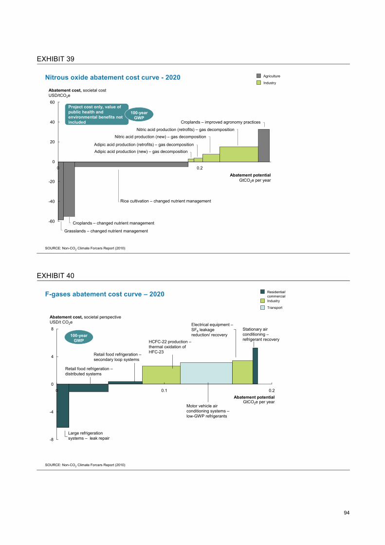
94

EXHIBIT 39

0

-60

-40

-20

60

Abatement cost, societal costUSD/tCO2e

40

0 0.2


20

Nitric acid production (retrofits) – gas decomposition


Nitric acid production (new) – gas decomposition


Grasslands – changed nutrient management

Croplands – changed nutrient management

Adipic acid production (new) – gas decompositionAdipic acid production (retrofits) – gas decomposition

Agriculture

Industry


Nitrous oxide abatement cost curve - 2020


100-year GWP

Updated 100701

EXHIBIT 40

F-gases abatement cost curve – 2020

0.10

8

-4

0.2

4

0


Abatement cost, societal perspectiveUSD/t CO2e

-8

HCFC-22 production –thermal oxidation of HFC-23


Residential/commercialIndustry

Transport

Large refrigeration systems – leak repair

Retail food refrigeration –distributed systems

Retail food refrigeration –secondary loop systems

Stationary air conditioning –refrigerant recovery

Electrical equipment –SF6 leakage reduction/ recovery

Motor vehicle air conditioning systems –low-GWP refrigerants

100-year GWP

Updated 100701

95

EXHIBIT 41

Black carbon abatement cost curve – 2020 (GWP 100)

90807060

10

100

130

2030

110120

40

0 0.50


-30-20

50

-10

-40


Industry

Residential

Transport


Tunnel Kilns replacing BTK & IDK

VSBK replacing BTK & IDKVSBK replacing Clamp Kilns

Improved cookstoves


LPG cookstoves (replacing traditional coal stoves)

MDV Diesel US 04/Euro 5 controls

LDV Gasoline Euro 4 equivalent controls

LDDV particulate filters, new (Euro 5)

2-/3-wheeler TWCHDV Diesel US 04 / Euro 5 equivalent controls



HDV DPF, retrofits


Agricultural machinery, stage 2 controls


Tunnel Kilns replacing Clamp Kilns




100-year GWP

EXHIBIT 42

Black carbon abatement cost curve – 2020 (GWP 20)

1.51.00.5Abatement potential

GtCO2e per year

0

10

20

30

40

-10


2.0

-15

-5

5

15

25

35

Transport

Industry

Residential


Tunnel Kilns replacing BTK & IDK

VSBK replacing BTK & IDKVSBK replacing Clamp Kilns

Improved cookstoves


LPG cookstoves (replacing traditional coal stoves)MDV Diesel US 04/Euro 5 controls

LDV Gasoline Euro 4 equivalent controls

LDDV particulate filters, new (Euro 5)

2-/3-wheeler TWCHDV Diesel US 04 / Euro 05 equivalent controls



HDV DPF, retrofits


Agricultural machinery, stage 2 controls


Tunnel Kilns replacing Clamp Kilns




20-year GWP

96

Appendix D: Black and organic carbon in tonnes EXHIBIT 43

Business-as-usual emissions, 2005 - 2030

SOURCE: Non-CO2 Climate Forcers Report (2010); Bond inventory; Michael Walsh transport model; IIASA GAINS

Tons of black carbon emissions Tons of organic carbon emissionsGg BC Gg OC

Forestry

AgricultureWaste


Industry

Transport

2030

7.7

2.7

0.4 0

2.1

1.1

1.3

2005

8.0

2.7

0.3 0

2.1

1.2

1.7

Forestry

AgricultureWaste


IndustryTransport

2030

35.6

21.9

1.8 0

9.0

1.91.0

2005

34.1

21.2

1.6 0

8.4

1.71.1

Updated 100701

EXHIBIT 44

07812242426

3236444957

616985104104109

130552

LDDV Euro 4 equivalent controlsMDV Diesel US 04 / Euro 5 controlsLDDV particulate filters, new (Euro 5)VSBK replacing BTK & IDKConstruction machinery, stage 2 controlsP&G upstream - reduced flaringLDV Gasoline Euro 4 equivalent controlsTunnel Kilns replacing BTK & IDK

VSBK replacing Clamp KilnsAgricultural machinery, stage 2 controls1

Tunnel Kilns replacing Clamp Kilns1

HDV DPF, retrofitsMDV Gasoline Euro 4 controlsLPG cookstoves (replacing traditional coal stoves)Tunnel Kilns replacing VSBK

HDV particulate filters, new (Euro 6)Use of ESP in modern coke ovenHDV oxydation catalysts (US 04 / Euro 5)2-/3-wheeler TWCImproved cookstoves

Black carbonabatement in 2030, Gg BC

Organic carbon abatement in 2030, Gg OC

Black and Organic Carbon: Abatement potential by lever

Abatement lever

1,533Total 3,325Total


1 Largely CO2 abatement levers, and hence total potential is larger than shown here for N2O only

0-4

231764

837169

1866704898

25184

2172

2,606

Updated 100701

97

Appendix E: Areas of further research This report aims to provide a global perspective on the climate warming impact of four non-CO2 climate forcers using the best available research and data. There are, however, many areas of further study that would improve the understanding of total emissions, abatement potential, and costs. Four important areas for research are:

Climate effects of black carbon: Compared with the other forcers, the climate effects of black carbon and other aerosols are still not fully understood. Black carbon’s interactions with clouds and the subsequent impact on temperature are particularly unclear. (See sidebar “Climate effects of black carbon.”)

Emission factors: An accurate assessment of emission volumes depends upon knowing the emission factor—that is, the emission rate of a given forcer from a given source activity. This factor is then used along with knowledge about the frequency of that activity to calculate total volume emitted.

In the case of black carbon, for example, even apparently similar combustion technologies can result in different levels of black carbon emissions. More field measurements would be particularly valuable for understanding the emission factors of brick production, flaring in the petroleum and gas sectors, and newer cookstoves.

Most methane and nitrous oxide emissions emanate from biological processes, primarily in the agriculture and waste sectors, making them particularly difficult to measure. Regional and site-specific conditions affect the degree of anaerobic decomposition for methane, and nitrification and de-nitrification for nitrous oxide. More research and empirical data collection would be particularly valuable in the area of nutrient management and fertilizer use.

For f-gases, mainly HFCs, more research can go into the forecasting of technical solutions to be used after the phaseout of the ODSs (as the emissions factors measured in CO2e can differ by a factor of 10 or more when different HFCs are chosen for the same application). More research could also go into how energy efficiency (affected by climate conditions) and leak rates (affected by equipment handling) differ by region.

Additional benefits: More research would be needed to better understand the precise impact of different quantities of air pollutants on health, vegetation growth, and biodiversity (the dose-response function). The health and environmental effects of pollutants are particularly unclear in the developing world, where most harm is caused but fewer studies have been performed. There are also questions being raised concerning the linearity of dose-response functions, which need be resolved since models often assume this linearity.

98

Appendix F: Alternative metrics considerations

Excerpts from Final Report of IPCC Expert Meeting on the Science of Alternative Metrics Oslo, Norway – March 18-20, 2009

“Metrics are used to quantify a type of equivalence between CO2 emissions and emissions of other gases or aerosols. Metrics can be used to inform understanding of, and to communicate, the relative contribution to climate change of emissions (or reductions in emissions) of different gases or substances (e.g., CO2 versus non-CO2 gas contributions), or of emissions from different countries or sectors.” “The global warming potential (GWP) is a well established and well-defined physical metric that compares the integrated radiative forcing of two greenhouse gases over some chosen time period resulting from pulse emissions of an equal mass. The numerical value of the GWP can depend markedly on the choice of time horizon.” “The choice of metric type has the most impact when comparing emissions of gases with substantially different lifetimes. In practical terms, this means that, when comparing greenhouse gas emissions to CO2 emissions, the choice of metric and time horizon have much larger implications for methane than for nitrous oxide, whose lifetime is more similar to the lifetime of a CO2 perturbation. Specifying the time horizon imparts a value judgment by specifying the time period of importance.” “The short-lived nature of [some] pollutants poses additional challenges. For instance, even the global mean climate impacts for very short-lived pollutants can vary with the region of emission because of chemical, radiative, and dynamical effects. This spatial dependence further complicates comparison with CO2 emissions beyond the problems associated with comparing emissions of gases with dramatically different atmospheric residence times. Regional emissions of very short-lived pollutants may also result in regionally dependent outcomes so that a single global metric value may not be sufficient. In that case, it may be more appropriate to assign regionally dependent metric values to each type of emission.” “There are inherently fewer physical uncertainties in the metrics for long-lived non-CO2 greenhouse gases than there are for short lived species. A common source of uncertainty in metric values of long-lived greenhouse gases arises from the use of CO2 as the reference gas. While CO2 is chemically inert in the atmosphere, its behavior is complex because of the different removal processes and their timescales. Species with simpler removal terms such as SF6 and N2O have fewer uncertainties.” “For short-lived species, e.g., aerosols and ozone precursors, the transformation and sink terms are more complex than for most of the long-lived greenhouse gases. There is more sensitivity to background conditions because of non-linear effects, chemistry, and aerosol indirect effects. For NOx emissions, the nonlinearities in the chemistry and the sensitivity to

99

background conditions can result in a change in sign of the net forcing for some emissions, such as those from aircraft. In addition, radiative properties for some types of aerosols are not well constrained. Cloud processes are also not well characterized in terms of their response to short-lived species. Furthermore, because the oxidation of some carbon-containing species (CH4, CO, NMHCs) ultimately produces CO2, proper treatment of their sources (biogenic or fossil-fuel derived) can make a difference to some indices over long timescales.”

100

Appendix G: List of major assumptions BUSINESS-AS-USUAL EMISSIONS ASSUMPTIONS (sorted by climate forcer)

Methane

Sub-sector Key 2005 inventory sources/assumptions Key growth sources/assumptions

Sectors: Coal mining Landfills Wastewater Enteric fermentation Rice cultivation Manure management Other agriculture Biomass combustion Stationary & mobile combustion

Emissions based on US EPA Global Anthropogenic Emissions Report (2006)

US EPA’s emission estimates used for the period 2005-2020 2021-2030 emissions extrapolated based on the average 2015-2020 annual growth rate

Petroleum & Gas Midstream emissions based on McKinsey GHG Cost Curve v2.0 Flaring activity based on NOAA/ McKinsey GHG Cost Curve v2.0 Other upstream emissions based on McKinsey GHG Cost Curve v2.0 and US EPA Natural Gas STAR Program

Flaring activity based on NOAA/ McKinsey GHG Cost Curve v2.0 Other emissions grow according to growth rates in McKinsey GHG Cost Curve v2.0, in turn driven by oil and gas demand/supply projections by IEA

Nitrous oxide


Sectors: Agricultural soils Manure management Other agriculture Wastewater (includes human sewage only) Biomass combustion Stationary and mobile combustion


US EPA’s emission estimates used for the period 2005-2020

2021-2030 emissions extrapolated based on the average 2015-2020 annual growth rate

Chemicals Emissions based on McKinsey GHG Cost Curve v2.0, in turn relying on SRI

See 2005 inventory

F-gases


Non-ODS substitutes:

Aluminum production HFC-23 emissions from HCFC-22 production Magnesium production Semiconductor production SF6 emissions from electric power systems


US EPA’s emission estimates used for the period 2005-2020

2021-2030 emissions extrapolated based on the average 2015-2020 annual growth rate

ODS substitutes: Aerosols Fire extinguishing Foams Refrigeration and air conditioning Solvents


US EPA’s emission estimates used for the period 2005-2020 2021-2030 emissions extrapolated based on the average 2005-2020 annual growth rate for developing countries 2021-2030 emissions extrapolated based on the average 2015-2020 annual growth rate approaching

101

population growth rate for developed countries in 2030

Black carbon Sub-sector Key 2005 inventory sources/assumptions Key growth sources/assumptions Road Transport Approach and data based on Michael Walsh

transport model Total distance travelled and distance travelled per vehicle based on McKinsey GHG Cost Curve v2.0

See 2005 inventory

Off-road Transport Emissions based on IIASA's GAINS model See 2005 inventory Shipping Emissions derived from Corbett et al.

(2010) See 2005 inventory

Brick kilns Brick production based on UN Statistics Division, Maithel (2008), Air Pollutant Emission Standards for China Tile & Brick Industry (2009), and expert estimates Split in kiln types based on GAINS, expert estimates Emission factors from GAINS model

Brick production extrapolated based on based on construction growth projections, Air Pollutant Emission Standards for China Tile & Brick Industry (2009), and expert estimates Emission factors from GAINS model

Coke ovens Coke production based on Resource-Net Split in coke oven types and control technology penetration rates derived from GAINS, the Chinese “Guidance of Restructuring of Coking Industry 2006,” expert estimates Emission factors from GAINS model

Coke projection based on McKinsey Basic Materials Practice Split in coke oven types and control technology penetration rates derived from GAINS, the Chinese “Guidance of Restructuring of Coking Industry 2006,” expert estimates Emission factors from GAINS model

Petroleum & Gas Flaring activity based on NOAA/ McKinsey GHG Cost Curve v2.0 Emission factors from IIASA/Z. Klimont communication

Flaring activity based on NOAA/ McKinsey GHG Cost Curve v2.0 Emission factors from IIASA/Z. Klimont communication

Power generation Fuel consumption from IEA WEO 2009 Emission factors based on Tami Bond inventory (SPEW)

See 2005 inventory

Other industry Fuel consumption from IEA WEO 2009 Emission factors based on Tami Bond inventory (SPEW)

See 2005 inventory

Residential cook stoves Fuel consumption and type of cook stoves derived from GAINS, IEA, REN21 (2005), Fernandes et al (2007) Emission factors based on Tami Bond inventory (SPEW)

See 2005 inventory

Other residential & commercial Fuel consumption from IEA WEO 2009 Emission factors based on Tami Bond inventory (SPEW)

See 2005 inventory

Open waste burning Emissions based on Tami Bond inventory for 2000, extrapolated at population growth projections from IEA WEO 2009

See 2005 inventory

Open burning of crop residues Emissions based on Tami Bond inventory for 2000, extrapolated at cropland growth projections from McKinsey GHG Cost Curve v2.0

See 2005 inventory

Forest/savannah fires Emissions taken from GFEDv2.1 Average of emissions from 1998-2005 assumed from GFEDv2.1 for 2030 (corresponds to decline in deforestation rates from McKinsey GHG Cost Curve v2.0)

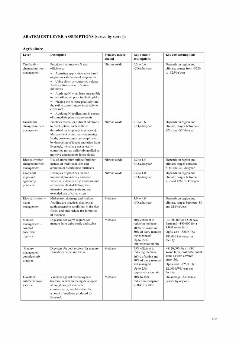
102

ABATEMENT LEVER ASSUMPTIONS (sorted by sector): Agriculture Lever Description Primary forcer

abated Key volume assumptions

Key cost assumptions

Croplands – changed nutrient management

Practices that improve N use efficiency: Adjusting application rates based on precise estimation of crop needs Using slow- or controlled-release fertilizer forms or nitrification inhibitors Applying N when least susceptible to loss, often just prior to plant uptake Placing the N more precisely into the soil to make it more accessible to crops roots Avoiding N applications in excess of immediate plant requirements

Nitrous oxide 0.3 to 0.6 tCO2e/ha/year

Depends on region and climate; ranges from -$220 to -$25/ha/year

Grasslands – changed nutrient management

Practices that tailor nutrient additions to plant uptake, such as those described for croplands (see above). Management of nutrients on grazing lands, however, may be complicated by deposition of faeces and urine from livestock, which are not as easily controlled nor as uniformly applied as nutritive amendments in croplands


Depends on region and climate; ranges between -$220 and -$25/ha/year


Use of ammonium sulfate fertilizer instead of traditional urea and ammonium bicarbonate fertilizers


Depends on region and climate; ranges between -$180 and -$30/ha/year


Examples of practices include improved productivity and crop varieties; extended crop rotations and reduced unplanted fallow; less intensive cropping systems; and extended use of cover crops


Depends on region and climate; ranges between $12 and $26 USD/ha/year

Rice cultivation – water management

Mid-season drainage and shallow flooding are practices that help to avoid anaerobic conditions in the rice fields, and thus reduce the formation of methane

Methane 4.0 to 4.9 tCO2e/ha/year

Depends on region and climate; ranges between -$8 and $12/ha/year

Manure management – covered anaerobic digester

Digesters for warm regions for manure from dairy cattle and swine

Methane 50% efficient in reducing methane 100% of swine and 50% of dairy manure wet managed Up to 25% implementation rate

~$160,000 for a 500 cow farm and ~$90,000 for a 1,000 swine farm OpEx cost ~$20/tCO2e 185,000 kWh/year per facility

Manure management – complete mix digester

Digesters for cool regions for manure from dairy cattle and swine

Methane 75% efficient in reducing methane 100% of swine and 50% of dairy manure wet managed Up to 25% implementation rate

~$120,000 for a 1,000 swine farm, cost differential same as with covered anaerobic OpEx cost ~$25/tCO2e 12,000 kWh/year per facility


Vaccines against methanogenic bacteria, which are being developed although not yet available commercially, would reduce the amount of methane produced by livestock

Methane 10% to 15% reduction compared to BAU in 2030

On average ~$9/ tCO2e (varies by region)

103

Livestock – feed supplements

Propionate precursors reduce methane formation by acting as alternative hydrogen acceptors. But as response is elicited only at high doses, propionate precursors are quite expensive

Methane 5% to 7% reduction compared to BAU in 2030

On average ~$86/ tCO2e (varies by region)

Waste Lever Description Primary forcer



Landfill gas – direct use

Capture landfill gas and sell to a captive player

Methane LFG direct use is limited to a technical potential of 30% of all sites Capture rates over the lifetime of the landfill is assumed to be 75%

On average -$26/ tCO2e (varies by region due to different labor costs and gas prices)

Landfill gas – electricity generation

Capture landfill gas to generate electricity

Methane LFG electricity generation is limited to a technical potential of 80% of all sites Capture rates over the lifetime of the landfill is assumed to be 75%

On average $2/ tCO2e (varies by region due to different labor costs and electricity prices)


Produce compost through biological process where organic waste biodegrades

Methane Food: 1.0 tCO2e/ ton Yard trimming: 1.3 tCO2e/ ton Paper: 1.9 tCO2e/ ton Wood: 1.5 tCO2e/ ton Textiles: 1.2 tCO2e/ ton

CapEx ranges between $51 and $74/ tCO2e OpEx typically ~$20 USD/ tCO2e; varies by region Savings vary by region

Industrial wastewater – improved treatment

Introduction of anaerobic pre-treatment and gas capture at industries (e.g., pulp & paper, and food processing plants) that currently lack such equipment

Methane Reduction by ~50% of emissions from addressed plants by 2030

CapEx: ~$20/ m3 of wastewater treated annually OpEx: ~$0.90/ m3 of wastewater (varies by region) Savings depend on gas price in each region

Industry Lever Description Primary forcer



Adipic acid production – gas decomposition (new builds/ retrofits)

Decomposition of nitrous oxide (produced in the process of making adipic acid) into oxygen and nitrogen through the use of catalysts

Nitrous oxide ~80-90% capture rate without lever (regional) 98% capture rate with lever 10% implementation share in BAU; 100% in abatement case by 2030

CapEx: ~$15/ ton acid (new build) OpEx: ~$30/ ton acid

Nitric acid production – gas decomposition (new builds/ retrofits)

Applying filtering measures in order to decompose nitrous oxide from the tail gas of nitric acid production, where nitrous oxide is produced as a process emission

Nitrous oxide ~7-9 ton of nitrous oxide per megaton acid without lever (regional) ~1 ton of nitrous oxide per megaton acid with lever Not implemented in BAU; 100%

CapEx: ~$15/ ton acid OpEx: ~$15/ ton acid

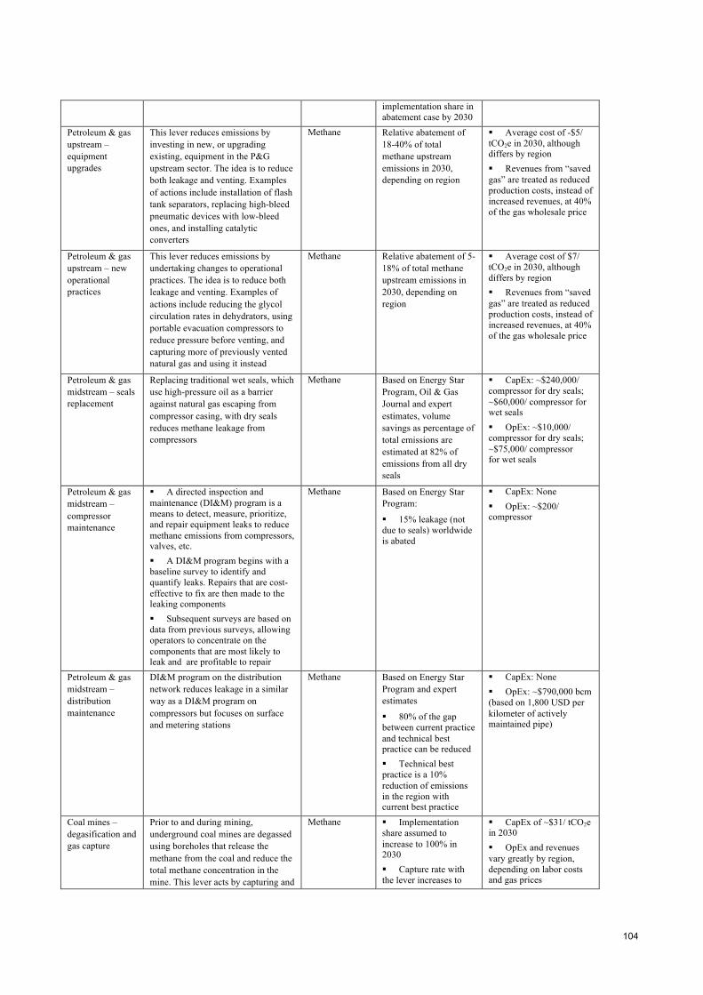
104

implementation share in abatement case by 2030

Petroleum & gas upstream – equipment upgrades

This lever reduces emissions by investing in new, or upgrading existing, equipment in the P&G upstream sector. The idea is to reduce both leakage and venting. Examples of actions include installation of flash tank separators, replacing high-bleed pneumatic devices with low-bleed ones, and installing catalytic converters

Methane Relative abatement of 18-40% of total methane upstream emissions in 2030, depending on region

Average cost of -$5/ tCO2e in 2030, although differs by region Revenues from “saved gas” are treated as reduced production costs, instead of increased revenues, at 40% of the gas wholesale price

Petroleum & gas upstream – new operational practices

This lever reduces emissions by undertaking changes to operational practices. The idea is to reduce both leakage and venting. Examples of actions include reducing the glycol circulation rates in dehydrators, using portable evacuation compressors to reduce pressure before venting, and capturing more of previously vented natural gas and using it instead

Methane Relative abatement of 5-18% of total methane upstream emissions in 2030, depending on region

Average cost of $7/ tCO2e in 2030, although differs by region Revenues from “saved gas” are treated as reduced production costs, instead of increased revenues, at 40% of the gas wholesale price

Petroleum & gas midstream – seals replacement

Replacing traditional wet seals, which use high-pressure oil as a barrier against natural gas escaping from compressor casing, with dry seals reduces methane leakage from compressors

Methane Based on Energy Star Program, Oil & Gas Journal and expert estimates, volume savings as percentage of total emissions are estimated at 82% of emissions from all dry seals

CapEx: ~$240,000/ compressor for dry seals; ~$60,000/ compressor for wet seals OpEx: ~$10,000/ compressor for dry seals; ~$75,000/ compressor for wet seals

Petroleum & gas midstream – compressor maintenance

A directed inspection and maintenance (DI&M) program is a means to detect, measure, prioritize, and repair equipment leaks to reduce methane emissions from compressors, valves, etc. A DI&M program begins with a baseline survey to identify and quantify leaks. Repairs that are cost-effective to fix are then made to the leaking components Subsequent surveys are based on data from previous surveys, allowing operators to concentrate on the components that are most likely to leak and are profitable to repair

Methane Based on Energy Star Program:

15% leakage (not due to seals) worldwide is abated

CapEx: None OpEx: ~$200/ compressor

Petroleum & gas midstream – distribution maintenance

DI&M program on the distribution network reduces leakage in a similar way as a DI&M program on compressors but focuses on surface and metering stations

Methane Based on Energy Star Program and expert estimates

80% of the gap between current practice and technical best practice can be reduced Technical best practice is a 10% reduction of emissions in the region with current best practice

CapEx: None OpEx: ~$790,000 bcm (based on 1,800 USD per kilometer of actively maintained pipe)

Coal mines – degasification and gas capture

Prior to and during mining, underground coal mines are degassed using boreholes that release the methane from the coal and reduce the total methane concentration in the mine. This lever acts by capturing and

Methane Implementation share assumed to increase to 100% in 2030 Capture rate with the lever increases to

CapEx of ~$31/ tCO2e in 2030 OpEx and revenues vary greatly by region, depending on labor costs and gas prices

105

collecting the gas that is degassed, and thereafter using or selling it

80-85% in 2030 On average, the lever comes at a societal cost of -26 USD/ tCO2e

Coal mines – oxidation of ventilation air methane

Coal mines are constantly ventilated with gigantic fans that blow in fresh air and suck out air containing methane from the mine. This is because of safety reasons and otherwise deadly explosion risks. The concentration is too low to be sold as natural gas, however, the ventilation air methane can be oxidized to produce heat and electricity

Methane 20% of the ventilation air is captured in the oxidation unit in 2010; increases to 50% to 2030 98% of the methane that enters the oxidation unit is oxidized

CapEx decreases to ~$47/ tCO2e in 2030 OpEx and revenues vary greatly by region, depending on labor costs and gas prices On average, the lever comes at a societal cost of -$2/ tCO2e

HFC-23 emissions from HCFC-22 production – Thermal oxidation of HFC-23

The HFC-23 that is emitted as an unwanted by-product can be abated by adding a thermal oxidation unit that collects and destroys the HFC-23. It is also assumed that extra waste treatment is needed to treat products

F-gas (HFCs) Reduction efficiency is close to 100% when the unit is operating, but necessary downtime reduces overall efficiency to 90% Implementation rate is assumed to reach 100% but there is also a high implementation rate assumed in the BAU

CapEx per plant ~$8m in the developed world and ~$6m in the developing world (including investments for extra waste treatment) OpEx per plant ~$750,000(including extra opex for waste water treatment and supervision) HFC-23 emissions per plant: 400 t/ yr in developed world vs. 600 t/ yr in developing world due to higher emission factor in developing world (3% vs. 2%)

SF6 emissions from electric power systems – Leak reduction and recovery

Recovering and recycling gas at maintenance Leakage reduction and repair Refurbishment of equipment to reduce leakages

F-gas (SF6) Reduction efficiency 60%

CapEx ~$12/ ton CO2e reduced OpEx ~$4/ ton CO2e reduced in developed regions, scaled with labor cost index Cost savings of ~$8/ lb of SF6

Brick production – VSBKs replacing IDK/BTKs and clamp kilns

Construction of more energy efficient vertical shaft brick kilns (VSBK) instead of lower cost traditional kiln types

Black carbon 90% replacement assumed to be possible by 2030

Replacement only possible for new-builds, i.e. no retrofits/ replacements before end of useful life

Lifetime of 10 years

CapEx ~$10m/Mt bricks vs. ~$3.5m/Mt bricks for IDK/BTKs and clamp kilns

Labor/other OpEx only marginally higher

Fuel savings of 60-70%

Brick production – Tunnel kilns replacing IDK/BTKs, clamp kilns, VSBKs

Construction of more energy efficient, simple tunnel kilns instead of lower cost traditional kiln types

Black carbon Tunnel kilns restricted to locations in close proximity urban to areas due to their production profile

Penetration rates ~50-70% in 2030

Replacement only possible for new-builds, i.e. no retrofits/

CapEx ~$16-$18m/Mt bricks

Labor/other OpEx only marginally higher

Fuel savings of 65-75%

106

replacements before end of useful life

Lifetime 15 years


Installation of electrostatic precipitators (ESP) on coke ovens without control technology to capture process emissions

Black carbon Assumes 99% potential penetration rate by 2030

CapEx ~$1/ t coke

Incremental electricity demand 0.26 kWh/t coke

Byproduct dependent on region

Petroleum & Gas – Reduction of continuous, remote flaring

Measures to reduce continuous flaring by capturing the otherwise flared gas and bringing it to market, which will require

– Gas recovery and treating units for oil associated gasses

Pipeline network to transport the gas

Black carbon Baseline flaring reduced by 72% between 2005–30

Of remaining flares

– 90% assumed to be large enough for a gathering system

– 70% close enough for a transportation system

95% of flaring is from continuous flaring

CapEx

– € 320 million per BCM for the gathering system

– 50 km pipe per flare @ $0.5 million per km

Average flare size of 2 mscf per day

OpEx estimated at 15% of total required CapEx

Savings result from reduced indirect electricity

Residential/commercial Lever Description Primary forcer

abated Key volume assumptions Key cost assumptions

Refrigeration and air conditioning – Refrigerant recovery from stationary air conditioning

Recovery of gas from stationary air conditioning at disposal and handing it in for reclamation

F-gas (HFCs) Assumed to be widely practiced in BAU in the developed world, less so in the developing world Reduction efficiency 25% (disposal emissions for smaller equipment which is assumed to be the equipment from which gas is not recovered in the BAU)

CapEx ~$700 for a recovery unit that can be used for 125 jobs per year Labor cost of $75/ h in the US, scaled by labor cost index for other regions Recovery time ~10 min per unit, varying by type of equipment plus ~7.5 min handling time for handing gas into reclamation Reclamation cost ~$3/ lb

Refrigeration and air conditioning – Distributed systems in retail food refrigeration

Distributed systems in stationary commercial refrigeration can be made much smaller than the ones used for centralized systems. Furthermore, leakage is reduced by minimizing the length of refrigerant tubing and the number of fittings

F-gas (HFCs) Emission reduction efficiency approximately 90%, from reduced refrigerant charge and reduced leakage Installed into new units (15 year life time assumed to calculate turnover) Different implementation rates into new units in different regions (reaches ~40-50% in 2030). Developing world is assumed to use more distributed systems than secondary loop

Calculated by using an example (large) supermarket as base case. This base case has a capital cost of ~$160,000, uses a 1,633 kg charge of R-404A and consumes 1,200,000 kWh per year

5% increase in CapEx relative to reference system 5% increase in electricity consumption relative to reference system Cost savings from reduced refrigerant consumption (R-404A)

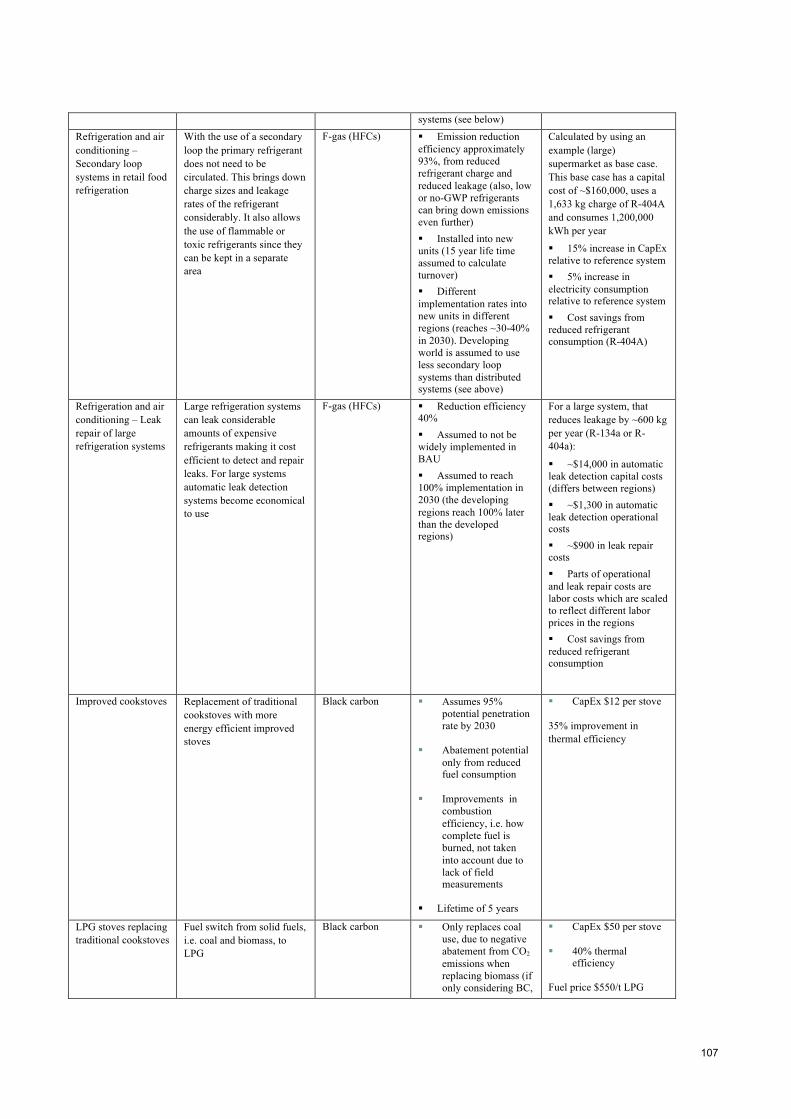
107

systems (see below) Refrigeration and air conditioning – Secondary loop systems in retail food refrigeration

With the use of a secondary loop the primary refrigerant does not need to be circulated. This brings down charge sizes and leakage rates of the refrigerant considerably. It also allows the use of flammable or toxic refrigerants since they can be kept in a separate area

F-gas (HFCs) Emission reduction efficiency approximately 93%, from reduced refrigerant charge and reduced leakage (also, low or no-GWP refrigerants can bring down emissions even further) Installed into new units (15 year life time assumed to calculate turnover) Different implementation rates into new units in different regions (reaches ~30-40% in 2030). Developing world is assumed to use less secondary loop systems than distributed systems (see above)

Calculated by using an example (large) supermarket as base case. This base case has a capital cost of ~$160,000, uses a 1,633 kg charge of R-404A and consumes 1,200,000 kWh per year

15% increase in CapEx relative to reference system 5% increase in electricity consumption relative to reference system Cost savings from reduced refrigerant consumption (R-404A)

Refrigeration and air conditioning – Leak repair of large refrigeration systems

Large refrigeration systems can leak considerable amounts of expensive refrigerants making it cost efficient to detect and repair leaks. For large systems automatic leak detection systems become economical to use

F-gas (HFCs) Reduction efficiency 40% Assumed to not be widely implemented in BAU Assumed to reach 100% implementation in 2030 (the developing regions reach 100% later than the developed regions)

For a large system, that reduces leakage by ~600 kg per year (R-134a or R-404a):

~$14,000 in automatic leak detection capital costs (differs between regions) ~$1,300 in automatic leak detection operational costs ~$900 in leak repair costs Parts of operational and leak repair costs are labor costs which are scaled to reflect different labor prices in the regions Cost savings from reduced refrigerant consumption

Improved cookstoves Replacement of traditional cookstoves with more energy efficient improved stoves

Black carbon Assumes 95% potential penetration rate by 2030

Abatement potential only from reduced fuel consumption

Improvements in combustion efficiency, i.e. how complete fuel is burned, not taken into account due to lack of field measurements

Lifetime of 5 years

CapEx $12 per stove

35% improvement in thermal efficiency

LPG stoves replacing traditional cookstoves

Fuel switch from solid fuels, i.e. coal and biomass, to LPG

Black carbon Only replaces coal use, due to negative abatement from CO2

emissions when replacing biomass (if only considering BC,

CapEx $50 per stove

40% thermal efficiency

Fuel price $550/t LPG

108

OC and CO2)

Lifetime of 5 years

Road transport

Lever Description Primary forcer abated

Key volume assumptions


Refrigeration and air conditioning – Low-GWP refrigerants in motor vehicle air conditioning

Switching refrigerants from HFC-134a (GWP of 1,300) to a refrigerant with GWP below 150 (as in EU style regulation) such as CO2, HFC-152a or HFO-1234yf Lever is calculated as one aggregated lever since there is no consensus on which alternative will be chosen by the industry and the industry will most likely stick to one alternative

GWP of alternatives is conservatively chosen to be 150, as this is the limit in EU regulations

F-gas (HFCs) ~90% reduction in emissions (going from 1,300 to 150 in GWP) Implementation into new sales can technically reach 100% in all regions, but penetration into total emissions is delayed due to the lifetime of the vehicles from previous periods

Incremental cost per vehicle ranges between ~$50-$75 15% reduction in fuel consumption, the baseline consumption differs between regions

LDV diesel oxydation catalysts, new (Euro 4)

Emission control technology to meet Euro 4 emission limits on new vehicles

Requires e.g., – Electric fuel timing &

metering – Electric EGR, with

cooling system – Direct injection (DI)

combustion and High pressure fuel injection (HPFI)

– Diesel Oxidation Catalyst (DOC)

Black carbon Introduced in 2015 in Africa and Other Non-OECD countries

Incremental CapEx of $260-$320/ vehicle in 2005 compared to vehicle with no emission controls

2.5% annual cost decrease

No change in OpEx

LDV diesel particulate filters, new (Euro 5)


Euro 4 equipment plus diesel particulate filte

Black carbon Introduced in 2015 in China, India, Latin America



No change in OpEx LDV gasoline particulate filters, new (Euro 4)


Requires e.g., – Elec. Injection, – Elec. ignition, – Multi-point injection

(MPI) – Second O2 sensor for

OBD – Three way catalyst

(underbody)

Black carbon Introduced in 2015 in Africa, China, India, Latin America, Other Non-OECD countries

Same BC emission levels as Euro 5 controls



No change in OpEx

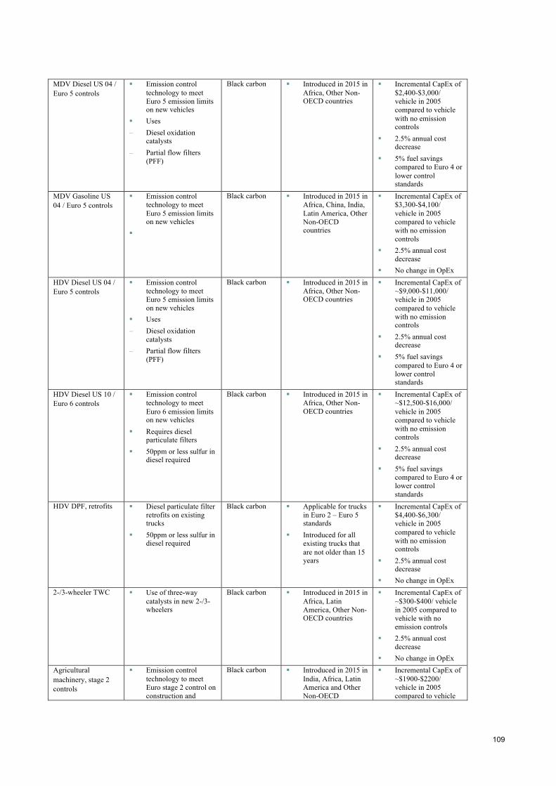
109

MDV Diesel US 04 / Euro 5 controls


Uses – Diesel oxidation

catalysts – Partial flow filters

(PFF)

Black carbon Introduced in 2015 in Africa, Other Non-OECD countries

Incremental CapEx of $2,400-$3,000/ vehicle in 2005 compared to vehicle with no emission controls


5% fuel savings compared to Euro 4 or lower control standards

MDV Gasoline US 04 / Euro 5 controls


Black carbon Introduced in 2015 in Africa, China, India, Latin America, Other Non-OECD countries



No change in OpEx HDV Diesel US 04 / Euro 5 controls


Uses – Diesel oxidation

catalysts – Partial flow filters

(PFF)


Incremental CapEx of ~$9,000-$11,000/ vehicle in 2005 compared to vehicle with no emission controls



HDV Diesel US 10 / Euro 6 controls


Requires diesel particulate filters

50ppm or less sulfur in diesel required


Incremental CapEx of ~$12,500-$16,000/ vehicle in 2005 compared to vehicle with no emission controls



HDV DPF, retrofits Diesel particulate filter retrofits on existing trucks

50ppm or less sulfur in diesel required

Black carbon Applicable for trucks in Euro 2 – Euro 5 standards

Introduced for all existing trucks that are not older than 15 years



No change in OpEx 2-/3-wheeler TWC Use of three-way

catalysts in new 2-/3-wheelers

Black carbon Introduced in 2015 in Africa, Latin America, Other Non-OECD countries

Incremental CapEx of ~$300-$400/ vehicle in 2005 compared to vehicle with no emission controls


No change in OpEx Agricultural machinery, stage 2 controls

Emission control technology to meet Euro stage 2 control on construction and

Black carbon Introduced in 2015 in India, Africa, Latin America and Other Non-OECD

Incremental CapEx of ~$1900-$2200/ vehicle in 2005 compared to vehicle

110

agriculture mobile sources

countries with no emission controls

Increase in OpEx of ~$47-$54/ vehicle in 2005 compared to vehicle with no emission controls

1% fuel penalty compared to vehicle with no emission controls


Emission control technology to meet Euro stage 2 control on construction and agriculture mobile sources

Black carbon Introduced in 2015 in India, Africa, Latin America and Other Non-OECD countries

Incremental CapEx of ~$1900-$2200/ vehicle in 2005 compared to vehicle with no emission controls

Increase in OpEx of ~$47-$54 USD/ vehicle in 2005 compared to vehicle with no emission controls

1% fuel penalty compared to vehicle with no emission controls

final report non-co2 climate forcers

Documents