caluniv.ac.infinal report of the major research project studies on two phase gas liquid (newtonian...
TRANSCRIPT

FINAL REPORT OF THE MAJOR RESEARCH PROJECT
STUDIES ON TWO PHASE GAS LIQUID (NEWTONIAN AND NON-NEWTONIAN) FLOW THROUGH PIPING COMPONENTS COILS AND FLOW
PHENOMENA USING CFD TECHNIQUE
UGC Reference No. : F-33-387/2007(S.R.) Dt. 29.02.2008
Submitted to
UNIVERSITY GRANTS COMMISSION
BAHADUR SHAH ZAFAR MARG
NEW DELHI – 110002
By
Dr. S. K. Das
Principal Investigator
Department of Chemical Engineering,
University of Calcutta,
92, A. P.C. Road, Kolkata-700009
UNIVERSITY GRANTS COMMISSION
BAHADUR SHAH ZAFAR MARG
NEW DELHI – 110002
Annual Report of the work done on the major research Project (report to be submitted within 6
weeks after completion of each year)
1. Project report No. 1st / 2
nd / Final : Final
2. UGC Reference No. : F-33-387/2007(S.R.) Dt. 29.02.2008
3. Period of report from : 1.7.2008 to30.06.2011 & 6 months extension
thereafter
4. Title of research project : Studies on Two Phase Gas Liquid (Newtonian and
Non-Newtonian) Flow through piping Components
coils and flow Phenomena using CFD Technique
5. (a) Name of the Principal Investigator : Dr.S.K. Das
(b) Dept. and University / College where work is progressed:
Department of Chemical Engineering,
University of Calcutta,
92, A. P.C. Road,
Kolkata-700009
6. Effective date of starting of the project : 1.7.2008
7. Grant approved and expenditure incurred during the period of the report :
Please see the Audited Statement of Account
8. Consolidated audited account :
Please see the Audited Statement of Account
9. Final Consolidated audited account certificate :
Please see the Audited Statement of Account
10. One copy of final progress report along with CD in pdf. Format
Attached
11. Details of expenditure incurred on Field Work duly signed and sealed by theRegistrar/Principal & Principal Investigator :
Not Applicable
12. Month-wise and Year-wise detailed statement of expenditure towards salary of staffappointed under the project :
Not Applicable
13. A Certificate from the Head of the Institute is mandatory that final report of the workdone has been kept in the library of the respective University/College and the executivesummary of the evaluated final report of work done on the project has been placed on thewebsite of the Institute :
Attached
14. HRA Certificate in the prescribed format, if applicable, duly signed by theRegistrar/Principal :
Not Applicable
15. Bank interest, if any, accrued by the Institution :
Please see in the audited statement of account
16. Refund unspent balance :

17. Ph.D. thesis completed
Tarun Kanti Bandyapadhyay - Studies on liquid and gas – liquid flow throughpiping components and coils using CFD technique, 2012
18. Report of the work done
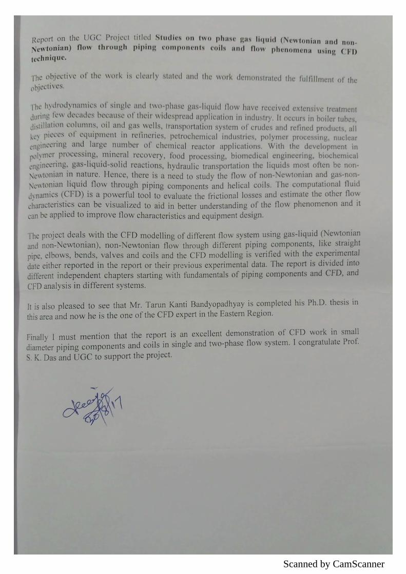
(a) Brief objective of the project:
(1) To generate the experimental data on the gas-non-Newtonian liquid flow throughhelical coils of different tube and coils diameters, different helix angles for verticalorientation.
(2) To generate the experimental data on the gas-non-Newtonian liquid flow throughhelical coils of different tube and coil diameters, different helix angles for horizontalorientation.
(3) The complex two-phase hydrodynamics was explained by using computational fluiddynamics, i.e. by Fluent 6.2 Software.
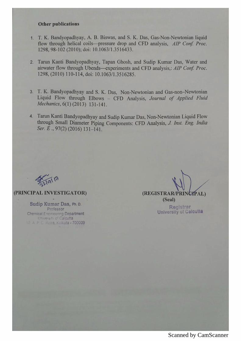
(b) Work done so far and results achieved and publication if any, resulting from the work(Give details of the title of the papers and names of the journal in which it has beenpublished or accepted for publication) :
(1) All experiments were completed and few data was analysed by CFD techniquesusing Fluent 6.2 Software.
(2) Studies on liquid and gas-liquid flow through piping components and coils usingCFD technique: Tarun Kanti Bandyapadhyay – Ph. D. completed, University ofCalcutta.
(3) Publications :
i. Ph. D. Thesis - Studies on liquid and gas – liquid flow through pipingcomponents and coils using CFD technique : Tarun Kanti Bandyopadhyay,2012.
Scanned by CamScanner

Scanned by CamScanner
Scanned by CamScanner

Scanned by CamScanner

Scanned by CamScanner

PREFACE
This is to certify that the project entitled Studies on Two Phase Gas Liquid (Newtonian
and Non-Newtonian) Flow through piping Components coils and flow Phenomena
using CFD Technique submitted by Dr. S. K. Das is submitted herewith. In the present
investigation some experimental studies have been carried out on the hydrodynamics of
single-phase and two-phase gas-liquid flow through piping components and coils and
some experimental data taken from earlier published report from our laboratory for the
simulation purpose. Commercial Fluent 6.3 software has been used for the simulation
purpose. The simulation gives the details flow field inside the piping components and
coils. The simulated results agree well with the experimental data.

CONTENTS
Page No.
Preface
Content 11
List of Tables vii
List of Figures
Synopsis
Chapter 1 In troduc t ion
1.1 Introduction
1.2 Objective of the present work
Chapter 2 CFD methodology
x
xxxix
2
6
2.1 Theoretical consideration 9
2.2 Mathematical model 10
2.2.1 Single phase water flow 10
2.2.2 Mathematical Model for Air - water system 11
2.3 Mathematical Model 12
2.3.l Single phase non-Newtonian fluid 12
2.3.2 For air-non-Newtonian fluid system 12
2.3.3 Estimation of the mesh cell size adjacent to the wall 15
2.4 Numerical approach 17
2.4.1 CFD procedure 17
2.4.2 Solver 19
Contents ii
2.4.3 Convergence 19
2.5 Conclusion 19
Chapter3 Water and air-waterflow throughU-bends
3.1 Introduction 22
3.2 The experimental set up 25
3.3 Evaluation of frictional pressure drop across the U-bend 26
3.4 CFD Procedure 27
3.4.1 Assumptions for air-water flow through U-bends 28
3.5 Results and discussion 29
3 .5 .1 Convergence and grid independency 29
3.5.2 CFD analysis for water flow through U-bends 30
3.5.3 CFD analysis for air-water flow through U-bends 34
3.6 Conclusions 37
Chapter 4 Non-Newtonian fluid flow throughpipingcomponents – experimentalinvestigation
4.1 Introduction 113
4.2 The experimental set up 115
4.3 Results and discussion 116
4.3.1 Evaluation of the pressure drop across the pipingcomponents
116
1174.3.2 Effect of non-Newtonian characteristics on thepressure drop across the piping components
4.3.3 Problem analysis 117
4.3.3.l Elbow 118
4.3.3.2 Orifice 119
Contents iii
4.3.3.3 Valves 120
4.3.4 Pressure drop 120
4.3.4.1 Analysis of the Experimental pressure drop 120
4.3.4.2 Stream-wise pressure drop due to pipe fittings 123
4.4 Conclusions 123
Chapter 5 Non-Newtonian liquid flow throughsmalldiameterpiping components - CFD analysis
5.1 Introduction 141
5.2 Experimental 143
5 .3 Mathematical Model 143
5 .4 CFD Procedure 144
5.5 Results and discussion 146
5.5.1 Convergence and grid independency 146
5.5.2 Straight pipe 147
5.5.3 Elbows 147
5.5.4 Orifices 150
5.5.5 Gate valve 150
5.5.6 Globe valve 151
5.6 Conclusions 151
Chapter 6 CFD analysis on two-phase gas-non-Newtonianliquid flow throughpiping components
6.1 Introduction 196
6.2 The Experimental setup 198
6.3 Mathematical Model 199
Contents iv
6.3.l CFD Procedure 199
6.3.2 Assumptions for air-SCMC flow through piping 201components
6.4 Results and discussion 202
6.4. l Convergence and grid independency 202
6.4.2 CFD analysis for air-non-Newtonian flow through 203straight pipe
6.4.3 Computational fluid dynamics (CFD) analysis 204for air-non-Newtonian liquid flow through elbows
6.4.4 CFD analysis for air-non-Newtonian liquid flow 206through orifices
6.4.5 CFD analysis for air-non-Newtonian flow through 207gate Valve
6.4.6 CFD analysis for air-non-Newtonian flow through 209globe Valve
6.5 Conclusions 210
Chapter 7 Non-Newtonian liquid flow throughhelical coils - CFD analysis
7.1 Introduction 283
7.2 The experimental setup 284
7.3 Mathematical Model 286
7.4 Computational fluid dynamics (CFD) Procedure 287
7.5 Results and discussion 289
7.5.1 Convergence and grid independency 289
7.5.2 Computational fluid dynamics (CFD) analysis 289
7.6 Comparison with the data available in the literature 293
7.7 Conclusions 294

vContents
Chapter 8 Gas-non-Newtonian liquid flowthrough helical coils - CFD analysis
8.1 Introduction 339
8.2 Experimental 341
8.3 Mathematical Model 342
8.3.1 CFD Procedure 342
8.3.2 Assumptions for air-SCMC flow through helical coils 344
8.4 Results and discussion 345
8.4.1 Convergence and grid independency 345
8.4.2 CFD analysis 346
8.5 Conclusions 351
Nomenclature 395
References 400

List of Tables
LIScIO(FcrmLcES
Table No. Title Page No.
2.1 General property $ for general transport equation 20
2.2 Empirical constants in K- e turbulence model 20
3.1 Dimensions of the U-bends used in the experiments 109
3.2 Range of variables used in the experiment 109
3.3 Comparison of the pressure drop across the U-bends, experimental and CFD analysis data
110
3.4 Comparison of the two-phase pressure drop across the U-bends, experimental and CFD analysis
111
4.1 Dimension of the piping components 138
4.2 Physical properties of the SCMC solution 138
4.3 Range of variables 139
5.1 Comparison of experimental and CFD analysis data for straight pipe
190
5.2 Comparison of experimental and CFD analysis data for elbows, Concentration of SCMC solution (kg/m3): 0.2
191
5.3 Comparison of experimental and CFD analysis data for orifice, Concentration of SCMC solution (kg/m3): 0.8
192
5.4 Comparison of experimental and CFD analysis data for gate valve, Concentration of SCMC solution (kg/m3): 0.8
193
5.5 Comparison of experimental and CFD analysis data 194

List of Tables viii
for globe valve, Concentration of SCMC solution (kg/m3): 0.8
6.1 Range of variables 272
6.2 Comparison of the experimental and CFD analysis 273data of two-phase pressure drop through straight pipefor different flow rate
6.3 Comparison of the experimental and CFD analysis 274 data of two-phase pressure drop through straight pipefor different SCMC concentration
6.4 Comparison of the experimental and CFD analysis 275data of two-phase pressure drop through elbows for different liquid flow rate
6.5 Comparison of the experimental and CFD analysis 276data of two-phase pressure drop through elbows at different elbow angle
6.6 Comparison of the experimental and CFD analysis 277data of two-phase pressure drop through orifices at different liquid flow rate
6.7 Comparison of the experimental and CFD analysis 278data of two-phase pressure drop through orifices at different orifice diameter ratio
6.8 Comparison of the experimental and CFD analysis 279data of two-phase pressure drop through gate valve at different flow rate
6.9 Comparison of the experimental and CFD analysis 280data of two-phase pressure drop at different openingof gate valve
6.10 Comparison of the experimental and CFD analysis 281data of two-phase pressure drop at different openingof globe valve
7.1 Range of variables investigated 334

List of Tables ix
7.2 Comparison of the experimental and CFD analysis 335data for the frictional pressure drop across the coil for different liquid concentration
7.3 Comparison of the experimental and CFD analysis 336data for frictional pressure across the coil for liquid concentration of 0.8 kg/m3 and different coil diameter
7.4 Comparison of the experimental and calculated data 337for friction factor across the coil for different liquid (SCMC) concentration
8.1 Range of variables investigated 391
8.2 Comparison of the experimental and CFD analysis 392data for frictional pressure drop across the coil forliquid (SCMC concentration) of 0.8 kg/m3
8.3 Comparison of the experimental and CFD analysis 393data for frictional pressure drop across the coil atdifferent liquid (SCMC) concentrations
8.4 Comparison of the experimental and CFD analysis 394data for frictional pressure drop across the coil forliquid (SCMC) concentration of 0.8 kg/m3 for different coil diameters
List of Figures
Figure No.
2.1
3.1
3.2
3.3
3.4
3.5
3.6
3.7
3.8
3.9
3.10
3.11
3.12
3.13
3.14
£IS‘TO‘F<FigVmS
Title
Discretized cell
Schematic diagram of experimental set up
Pressure distributions along pipeline with a bend
Typical static pressure distribution curve
Grid for U-bends
Plot of Velocity vector for U-bend for water velocity (m/s): 0.933
Plot of velocity vector in the bend portion i.e. helicity for U- bends for water velocity (m/s): 0.933
Contour plot of velocity vector at different points in the bend at water velocity (m/s): 0.933 and radius of curvature (m): 0.06
Contour plot of velocity vector at angular coordinates in the bend for water velocity (m/s): 0.933 and radius of curvature (m): 0.06
Contour plot of velocity at different points in the bend for water velocity (m/s): 0.933 and radius of curvature (m): 0.06
Contour plot of velocity at angular coordinates in the bend for water velocity (m/s): 0.933 and radius of curvature (m): 0.06
Contour plot of velocity at radial coordinates in the bend for water velocity (m/s): 0.933 and radius of curvature (m): 0.06
Contour plot of cell Reynolds number at different points in the bend for water velocity (m/s): 0.933 and radius of curvature (m): 0.06
Contour plot of cell Reynolds number at angular coordinates in the bend for water velocity (m/s): 0.933 and radius of curvature (m): 0.06
Contour plot of cell Reynolds number at radial coordinates in the bend for water velocity (m/s): 0.933 and radius of curvature (m): 0.06

List of Figures xi
3.15 Contour plot of tangential velocity at different points in the bend for water velocity (m/s): 0.933 and radius of curvature (m): 0.06
3.16 Contour plot of tangential velocity at angular coordinates in the bend for water velocity (m/s): 0.933 and radius of curvature (m): 0.06
3.17 Contour plot of radial velocity at different points in the bend for water velocity (m/s): 0.933 and radius of curvature (m): 0.06
3.18 Contour plot of radial velocity at angular coordinates in the bend for water velocity (m/s): 0.933 and radius of curvature (m): 0.06
3.19 Contours plot of static pressure for U-bend for water velocity (m/s): 0.933
3.20 Contour plot of static pressure at different points in the bend for water velocity (m/s): 0.933 and radius of curvature (m): 0.06
3.21 Contour plot of static pressure at angular coordinates in the bend for water velocity (m/s): 0.933 and radius of curvature (m): 0.06
3.22 Contour plot of static pressure at radial coordinates in the bend for water velocity (m/s): 0.933 and radius of curvature (m): 0.06
3.23 Contour velocity plot inside the different points of U-bend water velocity: 0.933 m/s, radius of curvature: 0.06 m
3.24 Contour velocity plot inside the different angular points of U- bend water velocity: 0.933 m/s, radius of curvature: 0.06 m
3.25 Experimental and CFD static pressure distribution
3.26 Contours plot of wall shear stress for U-bend for water velocity (m/s): 0.933
3.27 Contour plot of wall shear stress at different points in the bend water velocity: 0.933 m/s, radius of curvature: 0.06 m
3.28 Contour plot of wall shear stress at angular coordinates in the bend for water velocity (m/s): 0.933, radius of curvature(m): 0.06
3.29 Contour plot of wall shear stress at radial coordinates in the bend for water velocity (m/s): 0.933, radius of curvature(m): 0.06
3.30 Contours plot of strain rate for U-bend for water velocity (m/s):

List of Figures xii
0.9333.31 Contour plot of wall strain rate at different points in the bend for
water velocity (m/s): 0.933, radius of curvature(m): 0.06
3.32 Contour plot of strain rate at angular coordinates in the bend for water velocity (m/'s): 0.933, radius of curvature (m): 0.06
3.33 Contour plot of strain rate at radial coordinates in the bend for water velocity (m/s): 0.933, radius of curvature (m): 0.06
3.34 Contour plot of helicity at different points in the bend for water velocity (m/s): 0.933, radius of curvature (m): 0.06
3.35 Contour plot of helicity at angular coordinates in the bend for water velocity (m/s): 0.933, radius of curvature (m): 0.06
3.36 Contour plot of helicity at radial coordinates in the bend for water velocity (m/s): 0.933, radius of curvature (m): 0.06
3.37 Contour plot of vorticity at different points in the bend for water velocity (m/s): 0.933, radius of curvature (m): 0.06
3.38 Contour plot of vorticity at angular coordinates in the bend for water velocity (m/s): 0.933, radius of curvature (m): 0.06
3.39 Contour plot of vorticity at radial coordinates in the bend for water velocity (m/s): 0.933, radius of curvature (m): 0.06
3.40 Contour plot of turbulent kinetic energy at different points in the bend for water velocity (m/s): 0.933, radius of curvature (m): 0.06
3.41 Contour plot of turbulent kinetic energy at angular coordinates in the bend for water velocity (m/s): 0.933, radius of curvature (m): 0.06
3.42 Contour plot of turbulent kinetic energy at radial coordinates in the bend for water velocity (m/s): 0.933, radius of curvature (m): 0.06
3.43 Contour plot of turbulent intensity at different points in the bend for water velocity (m/s): 0.933, radius of curvature (m): 0.06
3.44 Contour plot of turbulent intensity at angular coordinates in the bend for water velocity (m/s): 0.933, radius of curvature (m): 0.06
3.45 Contour plot of turbulent intensity at radial coordinates in the

List of Figures
3.46
3.47
3.48
3.49
3.50
3.51
3.52
3.53
3.54
3.55
3.56
3.57a
3.57b
xiii
bend for water velocity (m/s): 0.933, radius of curvature (m): 0.06
Contour plot of turbulent dissipation rate at different points in the bend for water velocity (m/s): 0.933, radius of curvature (m): 0.06
Contour plot of turbulent dissipation rate at angular coordinates in the bend for water velocity (m/s): 0.933, radius of curvature (m): 0.06
Contour plot of turbulent dissipation rate at radial coordinates in the bend for water velocity (m/s): 0.933, radius of curvature (m): 0.06
Contour plot of production of k at different points in the bend for water velocity (m/s): 0.933, radius of curvature (m): 0.06
Contour plot of production of k at angular coordinates in the bend for water velocity (m/s): 0.933, radius of curvature (m): 0.06
Contour plot of turbulent viscosity at different points in the bend for water velocity (m/s): 0.933, radius of curvature (m): 0.06
Contour plot of turbulent viscosity at angular coordinates in the bend for water velocity (m/s): 0.933, radius of curvature (m): 0.06
Contour plot of turbulent viscosity at radial coordinates in the bend for water velocity (m/s): 0.933, radius of curvature (m): 0.06
Contour plot of mass imbalance at radial coordinates in the bend for water velocity (m/s): 0.933, radius of curvature (m): 0.06
Comparison plot of the experimental data and CFD modeling for water flow
Contour plot of velocity vector for U-bend, water velocity (m/s): 0.933, gas velocity (m/s): 1.365, gas fraction, ag: 0.59
Contour plot of velocity vector for air-water mixture at different points in the bend, radius of curvature 0.06 m, water velocity (m/'s): 0.933, gas velocity (mi/s): 1.365, gas fraction, aR: 0.59
Contour plot of velocity vector for water in the mixture at different points in the bend, radius of curvature 0.06 m, water velocity (m/s): 0.933, gas velocity (m/s): 1.365, gas fraction, ag:0.59
List of Figures xiv
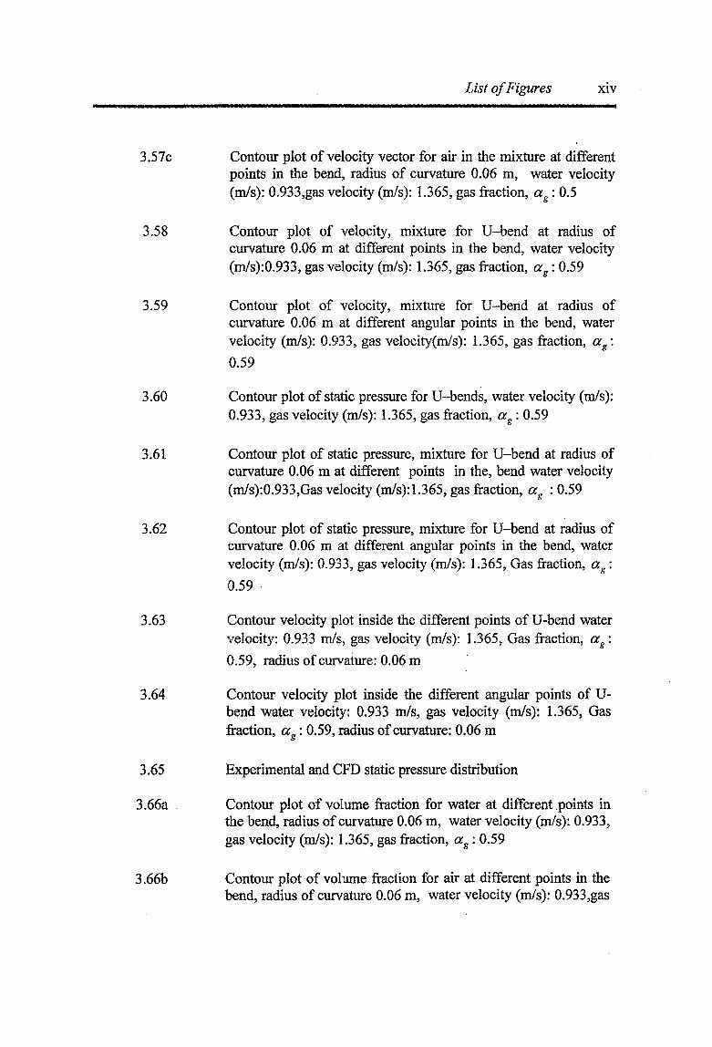
3.57c Contour plot of velocity vector for air in the mixture at differentpoints in the bend, radius of curvature 0.06 m, water velocity (m/s): 0.933,gas velocity (m/s): 1.365, gas fraction, ag: 0.5
3.58 Contour plot of velocity, mixture for U-bend at radius of curvature 0.06 m at different points in the bend, water velocity (m/s):0.933, gas velocity (m/s): 1.365, gas fraction, ag: 0.59
3.59 Contour plot of velocity, mixture for U-bend at radius of curvature 0.06 m at different angular points in the bend, water velocity (m/s): 0.933, gas veloeity(m/s): 1.365, gas fraction, ag: 0.59
3.60 Contour plot of static pressure for U-bends, water velocity (m/s): 0.933, gas velocity (m/s): 1.365, gas fraction, ag: 0.59
3.61 Contour plot of static pressure, mixture for U-bend at radius of curvature 0.06 m at different points in the, bend water velocity (m/s):0.933,Gas velocity (m/s): 1.365, gas fraction, ag : 0.59
3.62 Contour plot of static pressure, mixture for U-bend at radius of curvature 0.06 m at different angular points in the bend, water velocity (m/s): 0.933, gas velocity (m/s): 1.365, Gas fraction, ag:0.59
3.63 Contour velocity plot inside the different points of U-bend water velocity: 0.933 m/s, gas velocity (m/s): 1.365, Gas fraction, ag: 0.59, radius of curvature: 0.06 m
3.64 Contour velocity plot inside the different angular points of U- bend water velocity: 0.933 m/s, gas velocity (m/s): 1.365, Gas fraction, ag: 0.59, radius of curvature: 0.06 m
3.65 Experimental and CFD static pressure distribution
3.66a Contour plot of volume fraction for water at different points inthe bend, radius of curvature 0.06 m, water velocity (m/s): 0.933, gas velocity (m/s): 1.365, gas fraction, ag: 0.59
3.66b Contour plot of volume fraction for air at different points in thebend, radius of curvature 0.06 m, water velocity (m/s): 0.933,gas

List of Figures xv
velocity (m/s): 1.365, gas fraction, ag: 0.59
3.67a Contour plot of volume fraction for water at different angularpoints in the bend, radius of curvature 0.06 m, water velocity (m/s): 0.933, gas velocity (m/s): 1.365, gas fraction, ag: 0.59
3.67b Contour plot of volume fraction for air at angular coordinates inthe bend, radius of curvature 0.06 m, water velocity (m/s): 0.933,gas velocity (m/s): 1.365, gas fraction, a„: 0.59
©
3.68 Contour plot of shear stress and shear strain for U-bend at radius of curvature 0.06 m at different points in the bend, water velocity (m/s): 0.933, Gas velocity (m/s): 1.365, Gas fraction, ag : 0.59
3.69 Comparison plot of the experimental data and CFD modeling for two - phase air-water flow
3.70 Comparison of the two-phase pressure drop across the U-bends, experimental and CFD analysis
4.1 Schematic diagram of the experimental setup
4.2 Static pressure distribution curve across the valve
4.3 Typical static pressure distribution curve for elbow
4.4 Typical static pressure distribution curve for orifice
4.5 Typical static pressure distribution curve for gate valve
4.6 Typical static pressure distribution curve for globe valve
4.7 Variation of the pressure drop across the elbow with liquid flow rate
4.8 Variation of the pressure drop across the orifice with liquid flow rate
4.9 Variation of the pressure drop across the gate valve with liquid flow rate
4.10 Variation of the pressure drop across the globe valve with liquid flow rate
4.11 Comparison of the experimental pressure drop across 45° elbow

List of Figures xvi
4.12
4.13
4.14
5.1
5.2
5.3
5.4
5.5
5.6
with Turian et al. (1998) correlation
Comparison of the experimental pressure drop across 90° elbow with Edwards et al. (1985) and Telis-Romero et al. (2000) correlation
Comparison of the experimental pressure drop across gate valve with Edwards et al. (1985) and Turian et al. (1998) correlation
Comparison of the experimental pressure drop across globe valve with Edwards et al. (1985) and Turian et al. (1998) correlation Unstructured boundary layer hexahedral grid of straight pipe Grid Size: No. of cells = 200633; No. of faces = 615032, No. of nodes = 214428,1 cell zone, 4 face zones
Contour plot of static pressure for straight pipe Concentration of SCMC (kg/m3): 0.8,Liquid velocity (m/s):
0.3199
Plot of velocity vector for straight pipeConcentration of SCMC (kg/m3): 0.8, Liquid velocity (m/s): 0.3199Comparison of the experimental data and CFD modeling for straight pipe
Mesh geometry - unstructured t-grid (tetrahedral)(a) 45° elbow
Grid Size: No. of cells = 25985; No. of faces = 57149, No. of nodes = 7310,1 cell zone, 4 face zones(b) 90° elbow
Grid Size: No. of cells = 29157; No. of faces = 64167, No. of nodes = 8208,1 cell zone, 4 face zones(c) 135 0 elbow
Grid Size: No. of cells = 4427; No. of faces = 9778, No. of nodes = 1279,1 cell zone, 4 face zones(d)
Plot of velocity vector(a) 45° elbowConcentration of SCMC solution (kg/m3): 0.2, Liquid velocity (m/s): 0.296(b) 900 elbowConcentration of SCMC solution (Kg/m3): 0.2, Liquid velocity (m/s): 0.296 m/s(c) 135 0 elbowConcentration of SCMC solution (Kg/m3): 0.8, Liquid velocity (m/s): 1.733m/s

List of Figures xvii
5.7a
5.7b
5.7c
5.8a
5.8b
5.8c
5.9a
5.9b
5.9c
5.10
Contours plot of velocity vector inside the different points of 45° elbow, Concentration of SCMC solution (kg/m3): 0.8, Liquid flow rate, Qi(m3/s): 21.94xl0'5, Liquid velocity, V|(m/s): 1.733
Contour plot of velocity vector inside the different points of 90° elbow, Concentration of SCMC solution (kg/m3): 0.8, Liquid flowrate, Qi(m3/s): 21.94xl0'5, Liquid velocity, V|(m/s): 1.733
Contour plot of velocity vector inside the different points of 135° elbow, Concentration of SCMC solution (kg/m3): 0.8, Liquid flow rate, Qi (m3/s): 21.94xl0‘5, Liquid velocity, V\ (m/s): 1.733
Contours plot of velocity magnitude inside the different points of 45° elbow, Concentration of SCMC solution (kg/m3): 0.8, Liquid flow rate, Qi (m3/s): 21.94x10°, Liquid velocity, V| (m/s): 1.733
Contour plot of velocity magnitude inside the different points of 90° elbow, Concentration of SCMC solution (kg/m3): 0.8, Liquid flow rate, Qi (m3/s): 21.94xl0*5, Liquid velocity, V) (m/s): 1.733
Contour plot of velocity magnitude inside the different points of 135° elbow, Concentration of SCMC solution (kg/m3): 0.8, Liquid flow rate, Qi (m3/s): 21.94x10‘5, Liquid velocity, Vi (m/s): 1.733
Contour plot of X-velocity inside the different points of 45° elbow, Concentration of SCMC solution (kg/m3): 0.8, Liquid flow rate, Qi (m3/s): 21.94x10‘5, Liquid velocity, Vj (m/s): 1.733
Contour plot of X-velocity inside the different points of 90° elbow, Concentration of SCMC solution (kg/m3): 0.8, Liquid flowrate, Qi(m3/s): 21.94xl0'5, Liquid velocity, V|(m/s): 1.733
Contour plot of X-velocity inside the different points of 135° elbow, Concentration of SCMC solution (kg/m3): 0.8, Liquid flow rate, Qi (m3/s): 21.94xl0'5, Liquid velocity, V| (m/s): 1.733
Contour plot of static pressure(a) 45° elbowConcentration of SCMC solution (kg/m3): 0.2, Liquid velocity (m/s): 0.296(b) 90° elbowConcentration of SCMC solution (Kg/m3): 0.2 Liquid velocity (m/s): 0.296(c) 135 0 elbowConcentration of SCMC solution (Kg/m3): 0.4, Liquid velocity
List of Figures XV1X1
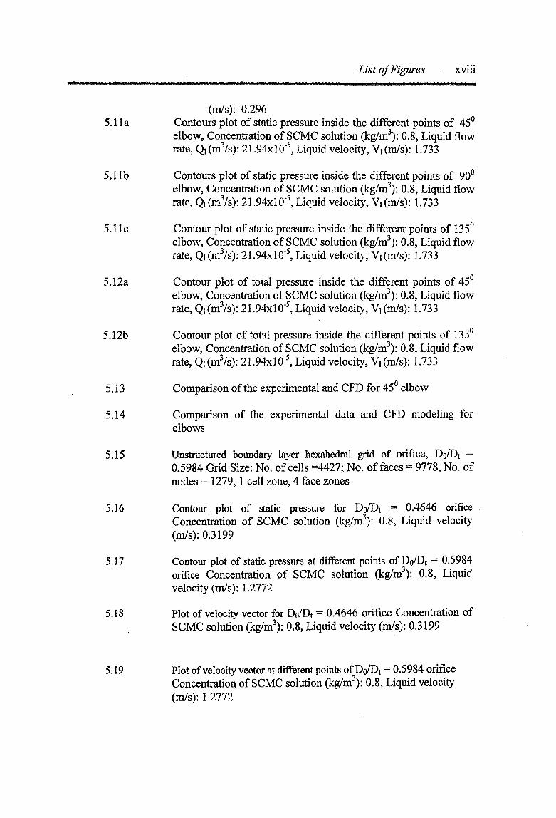
(m/s): 0.2965.1 la Contours plot of static pressure inside the different points of 45°
elbow, Concentration of SCMC solution (kg/m3): 0.8, Liquid flow rate, Qi (m3/s): 21.94xl0"5, Liquid velocity, Vi (m/s): 1.733
5.1 lb Contours plot of static pressure inside the different points of 90°elbow, Concentration of SCMC solution (kg/m3): 0.8, Liquid flow rate, Qi (m3/s): 21.94x1 O'5, Liquid velocity, V) (m/s): 1.733
5.11c Contour plot of static pressure inside the different points of 135°elbow, Concentration of SCMC solution (kg/m3): 0.8, Liquid flow rate, Qi(m3/s): 21.94xl0'5, Liquid velocity, V|(m/s): 1.733
5.12a Contour plot of total pressure inside the different points of 45°elbow, Concentration of SCMC solution (kg/m3): 0.8, Liquid flow rate, Qi (m3/s): 21.94x10'5, Liquid velocity, Vi (m/s): 1.733
5.12b Contour plot of total pressure inside the different points of 135°elbow, Concentration of SCMC solution (kg/m3): 0.8, Liquid flow rate, Qi (m3/s): 21.94xl0'5, Liquid velocity, V) (m/s): 1.733
5.13 Comparison of the experimental and CFD for 45° elbow
5.14 Comparison of the experimental data and CFD modeling for elbows
5.15 Unstructured boundary layer hexahedral grid of orifice, Do/Dt = 0.5984 Grid Size: No. of cells =4427; No. of faces = 9778, No. of nodes = 1279,1 cell zone, 4 face zones
5.16 Contour plot of static pressure for Do/Dt = 0.4646 orifice Concentration of SCMC solution (kg/m3): 0.8, Liquid velocity (m/s): 0.3199
5.17 Contour plot of static pressure at different points of Do/Dt = 0.5984 orifice Concentration of SCMC solution (kg/m3): 0.8, Liquid velocity (m/s): 1.2772
5.18 Plot of velocity vector for Do/Dt = 0.4646 orifice Concentration of SCMC solution (kg/m3): 0.8, Liquid velocity (m/s): 0.3199
5.19 Plot of velocity vector at different points of Do/Dt — 0.5984 orificeConcentration of SCMC solution (kg/m3): 0.8, Liquid velocity (m/s): 1.2772

List of Figures xix
5-20 Plot of velocity magnitude for Do/Dt = 0.59B4 orifice Concentrationof SCMC solution (kg/m3): 0.8, Liquid velocity (m/s): 1.2772
5.21 Comparison plot of experimental and CFD for orifice
5.22 Comparison of the experimental data and CFD modeling for orifices
5.23 Grid for 50% opening gate valve
5.24 Plot of static pressure for 50% opening gate valve Concentration of SCMC solution (kg/m3): 0.8, Liquid velocity (m/s): 1.5142
5.25 Plot of total pressure for 50% opening gate valve Concentration of SCMC solution (kg/m3): 0.8, Liquid velocity (m/s): 1.5142
5.26 Plot of velocity magnitude for 50% opening gate valve Concentration of SCMC solution (kg/m3): 0.8, Liquid velocity (m/s): 1.5142
5.27 Plot of velocity vector for 50% opening gate valve Concentration of SCMC solution (kg/m3): 0.8, Liquid velocity (m/s): 0.8033
5.28 Comparison plot of experimental and CFD for gate valve
5.29 Comparison of the experimental data and CFD modeling for gate valves
5.30 Unstructured boundary layer hexahedral grid of 75% opening globe valve Grid Size: No. of cells =348633; No. of faces = 1077668, No. of nodes = 381741,1 cell zone, 4 face zones
5.31 Plot of velocity vector for 75% opening globe valve Concentration of SCMC solution (kg/m3): 0.8, Liquid velocity (m/s): 0.8033
5.32 Comparison plot of experimental and CFD for globe valve
5.33 Comparison of the experimental data and CFD modeling for globe valves
6.1 Schematic diagram of the experimental setup

List of Figures xx
6.2 Contour plot of velocity vector in the air-SCMC mixture at different points of straight pipe, concentration of SCMC solution (kg/m3): 0.8, Liquid velocity (m/s): 1.2772, Gas velocity (m/s):1.9842, Gas fraction, ag: 0.3086
6.3 Plot of velocity vector for SCMC phase in the mixture at different points of straight pipe, concentration of SCMC solution (kg/m3): 0.8, Liquid velocity (m/s): 1.2772, Gas velocity (m/s): 1.9842, Gas fraction, ag: 0.3086
6-4 Contour plot of velocity vector for air phase in the mixture atdifferent points of straight pipe, concentration of SCMC solution (kg/m3): 0.8, Liquid velocity (m/s): 1.2772, Gas velocity (m/s):1.9842, Gas fraction, ag: 0.3086
6.5 Contour plot of velocity magnitude in air-SCMC mixture at different points of straight pipe, concentration of SCMC solution (kg/m3): 0.8, Liquid velocity (m/s): 1.2772, Gas velocity (m/s):1.9842, Gas fraction, ag: 0.3086
6.6 Contour plot of axial velocity inside the different points of straight pipe, concentration of SCMC solution (kg/m3): 0.8, Liquid velocity (m/s): 1.2772, Gas velocity (m/s): 1.9842, Gas fraction, ag: 0.3086
6.7 Contours of static pressure inside the different points of straight pipe, concentration of SCMC solution (kg/m3): 0.8, Liquid velocity (m/s): 1.2772, Gas velocity (m/s): 1.9842, Gas fraction, <zg: 0.3086
6.8 Contours of total pressure inside the different points of straight pipe, concentration of SCMC solution (kg/m3): 0.8, Liquid velocity (m/s): 1.2772, Gas velocity (m/s): 1.9842, Gas fraction, ag: 0.3086
6.9 Contours of SCMC phase volume fraction at different points of straight pipe, concentration of SCMC solution (kg/m3): 0.8, Liquid velocity (m/s): 1.2772, Gas velocity (m/s): 1.9842, Gas fraction, ag: 0.3086
6.10 Contours of air phase volume fraction at different points of

List of Figures xxi
straight pipe, concentration of SCMC solution (kg/m3): 0.8, Liquid velocity (m/s): 1.2772, Gas velocity (m/s): 1.9842, Gas fraction, ag: 0.3086
6.11 Comparison of the experimental data and CFD modeling for straight pipe varying with liquid flow rate
6.12 Comparison of the experimental data and CFD modeling for straight pipe varying with SCMC solution concentration
6.13 Comparison of experimental results with CFD simulated results for different liquid flow rate
6.14 Contour plot of velocity vector for air-SCMC mixture at different points in 45° elbow, concentration of SCMC solution (kg/m3): 0.8, Liquid velocity (m/s): 1.733, Gas velocity (m/s): 3.167, Gas fraction, ag: 0.64
6.15 Contour plot of velocity in the air-SCMC mixture at different points of elbows, concentration of SCMC solution (kg/m3): 0.8, Liquid velocity (m/s): 1.733 (a) 45°, Gas velocity (m/s): 3.167, Gas fraction, ag: 0.64 (b) 90°, Gas velocity (m/s): 2.3933, Gasfraction, ag: 0.58 (c) 135°, Gas velocity (m/s): 2.867, Gas
fraction, ag: 0.62
6.16 Contour plot of velocity vector for SCMC in the mixture at different points in 45° elbow, concentration of SCMC solution (kg/m3): 0.8, Liquid velocity (m/s): 1.733, Gas velocity (m/s): 3.167, Gas fraction, ag: 0.64
6.17 Contour plot of velocity vector for air in the mixture at different points in 90° elbow, concentration of SCMC solution (kg/m3): 0.8, Liquid velocity (m/s): 1.733, Gas velocity (m/s): 2.3933, Gas fraction, ag: 0.5
6.18 Contours plot of static pressure for elbows, concentration of SCMC solution (kg/m3): 0.8, liquid velocity (m/s): 1.733 (a) 45°, Gas velocity (m/s): 3.167, Gas fraction, ag: 0.64 (b) 90°, Gasvelocity (m/s): 2.3933, Gas fraction, ag: 0.58 (c) 135°, Gas
velocity (m/s): 2.867, Gas fraction, ag: 0.62

List of Figures xxii
6.19 Contour plot of static pressure, at different points in the elbows, concentration of SCMC solution (kg/m3): 0.8, Liquid velocity (m/s): 1.733 (a) 45°, Gas velocity (m/s): 3.167, Gas fraction, a„: 0.64(b) 90°, Gas velocity (m/s): 2.3933, Gas fraction, ag: 0.58(c) 135°, Gas velocity (m/s): 2.867, Gas fraction, ag: 0.62
6.20 Contour velocity plot inside different points of 45° elbow concentration of SCMC solution (kg/m3): 0.8, Liquid velocity (m/s): 1.733,Gas velocity (m/s): 3.167, Gas fraction, ag: 0.64
6.21 Contours of volume fraction for 90° elbow, concentration of SCMC solution (kg/m3): 0.8, Liquid velocity (m/s): 1.733, gas velocity (m/s): 2.3933, gas fraction, ag: 0.58 (a) SCMC phase and (b) air phase
6.22 Comparison plot of static pressure experimental and CFD for 45° elbow
6.23 Comparison of experimental results with CFD simulated results at different elbow angle
6.24 Contour plot of velocity vector for Do/Dt = 0.4646 orifice Concentration of SCMC solution (kg/m3): 0.8, Liquid velocity (m/s): 0.8033, Gas velocity (m/s): 0.3552, Gas fraction, ag: 0.30
6.25 Contour plot of velocity vector for Do/Dt = 0.5984 orifice Concentration of SCMC solution (kg/m3): 0.8, Liquid velocity (m/s): 0.8033, Gas velocity (m/s): 0.3552, Gas fraction, ag: 0.30
6.26 Contour plot of velocity vector for Do/Dt = 0.7087 orifice Concentration of SCMC solution (kg/m3): 0.8, Liquid velocity (m/s): 1.2772, Gas velocity (m/s): 2.4304, Gas fraction, ag: 0.65
6.27 Contour plot of static pressure for Do/Dt = 0.4646 orifice Concentration of SCMC solution (kg/m3): 0.8, Liquid velocity (m/s): 0.8033, Gas velocity (m/s): 0.3552, Gas fraction, ag: 0.30
6.28 Contour plot of static pressure for Do/Dt = 0.5984 orifice Concentration of SCMC solution (kg/m3): 0.8, Liquid velocity

List of Figures xxiii
6.29
6.30
6.31
6.32
6.33
6.34
6.35
6.36
6.37
(m/s): 0.8033, Gas velocity (m/s): 0.3552, Gas fraction, ag: 0.30
Contour plot of static pressure for Do/Dt = 0.7087 orifice Concentration of SCMC solution (kg/m3): 0.8, Liquid velocity (m/s): 1.2772, Gas velocity (m/s): 2.4304, Gas fraction, ag: 0.65
Contour plot of velocity vector in air-SCMC mixture at different points for Do/Dt = 0.4646 orifice Concentration of SCMC solution (kg/m3): 0.8, Liquid velocity (m/s): 1.2772, Gas velocity (m/s): 1.1508, Gas fraction, ag: 0.46
Contour plot of velocity vector plot of SCMC-phase in the mixture at different points for Do/Dt = 0.4646 orifice Concentration of SCMC solution (kg/m3): 0.8, Liquid velocity (m/s): 1.2772, Gas velocity (m/s): 1.1508, Gas fraction, ag: 0.46
Contour plot of velocity vector plot of air-phase in the mixture at different points for Do/Dt = 0.4646 orifice Concentration of SCMC mixture (kg/m3): 0.8, Liquid velocity (m/s): 1.2772, Gas velocity (m/s): 1.1508, Gas fraction, ag: 0.46
Contours plot of velocity magnitude in the air-SCMC mixture at different points for Do/Dt = 0.4646 orifice Concentration of SCMC solution (kg/m3): 0.8, Liquid velocity (m/s): 1.2772, Gas velocity (m/s): 1.1508, Gas fraction, ag: 0.46
Contours plot of velocity in the air-SCMC mixture inside the different points for Do/Dt = 0.4646 orifice Concentration of SCMC solution (kg/m3): 0.8, Liquid velocity (m/s): 1.2772, Gas velocity (m/s): 1.1508, Gas fraction, ag: 0.46
Contours plot of static pressure in the air-SCMC mixture inside the different points for Do/Dt = 0.4646 orifice Concentration of SCMC solution (kg/m3): 0.8, Liquid velocity (m/s): 1.2772, Gas velocity (m/s): 1.1508, Gas fraction, ag: 0.46
Contours plot of total pressure in the air-SCMC mixture inside the different points for Do/Dt = 0.4646 orifice Concentration of SCMC solution (kg/m3): 0.8, Liquid velocity (m/s): 1.2772, Gas velocity (m/s): 1.1508, Gas fraction, ag: 0.46
Contours plot of SCMC phase volume fraction in the mixture inside the different points of Do/Dt = 0.4646 orifice Concentration of SCMC solution (kg/m3): 0.8, Liquid velocity (m/s): 1.2772, Gas velocity

List of Figures xxiv
(m/s): 1.1508, Gas fraction, ag: 0.46
6.38 Contours of air phase volume fraction in the mixture inside the different points of Do/Dt = 0.4646 orifice Concentration of SCMC solution (kg/m3): 0.8, Liquid velocity (m/s): 1.2772, Gas velocity (m/s): 1.1508, Gas fraction, ag: 0.46
6.39 Comparison of the experimental result with CFD simulated result with different liquid flow rate and fixed liquid concentration, fixed orifice dimension
6.40 Comparison of the experimental result with CFD simulated result with different orifice dimension and fixed liquid concentration, fixed liquid flow rate
6.41 Comparison of experimental results with CFD simulated results for different liquid flow rates
6.42 Comparison of experimental results with CFD simulated results for different Orifice diameter ratios
6.43 Contours plot of velocity vector in the air-SCMC mixture at the different points of 50% opening gate valve, Concentration of SCMC solution (kg/m3): 0.8, Liquid velocity (m/s): 1.5142, Gas velocity (m/s): 3.0516, Gas fraction, ag: 0.668
6.44 Contours plot of velocity magnitude in the air-SCMC mixture at the different points of 50% opening gate valve, Concentration of SCMC solution (kg/m3): 0.8, Liquid velocity (m/s): 1.5142, Gas velocity (m/s): 3.0516, Gas fraction, ag: 0.6683
6.45 Contours plot of velocity in the air-SCMC mixture at the different points of 50% opening gate valve, Concentration of SCMC solution (kg/m3): 0.8, Liquid velocity (m/s): 1.5142, Gas velocity (m/s): 3.0516, Gas fraction, ag: 0.6683
6.46 Contours plot of static pressure in the air-SCMC mixture at the different points of 50% opening gate valve, Concentration of SCMC solution (kg/m3): 0.8, Liquid velocity (m/s): 1.5142, Gas velocity (m/s): 3.0516, Gas fraction, ag: 0.6683
6.47 Contours plot of total pressure in the air-SCMC mixture at the different points of 50% opening gate valve, Concentration of SCMC solution (kg/m3): 0.8, Liquid velocity (m/s): 1.5142, Gas velocity (m/s): 3.0516, Gas fraction, ag: 0.6683

List of Figures xxv
6.48 Contours plot of SCMC phase volume fraction in the air-SCMC mixture at the different points of 50% opening gate valve, Concentration of SCMC solution (kg/m3): 0.8, Liquid velocity (m/s): 1.5142, Gas velocity (m/s): 3.0516, Gas fraction, a°: 0.6683
6.49 Contours plot of air phase volume fraction in the air-SCMC mixture at the different points of 50% opening gate valve, Concentration of SCMC solution (kg/m3): 0.8, Liquid velocity (m/s): 1.5142, Gas velocity (m/s): 3.0516* Gas fraction, ag: 0.6683
6.50 Comparison of experimental results with CFD simulated results for different liquid flow rates
6.51 Comparison of experimental results with CFD simulated results for different % opening of Gate valve
6.52 Contours plot of velocity vector in the air-SCMC mixture for 50% opening globe valve, Concentration of SCMC solution (kg/m3): 0.8, Liquid velocity (m/s): 1.5142, Gas velocity (m/s): 1.7265, Gas fraction, ag: 0.5
6.53 Contours plot of velocity vector in the air-SCMC mixture at the different points of 50% opening globe valve, Concentration of SCMC solution (kg/m3): 0.8, Liquid velocity (m/s): 1.5142, Gas velocity (m/s): 1.7265, Gas fraction, ag: 0.5
6.54 Contours plot of velocity vector for SCMC phase in the air- SCMC mixture at the different points of 50% opening globe valve, Concentration of SCMC solution (kg/m3): 0.8, Liquid velocity (m/s): 1.5142, Gas Velocity (m/s): 1.7265, Gas fraction, cu: 0.5
6.55 Contours plot of velocity vector for air phase in the air-SCMC mixture at the different points of 50% opening globe valve, Concentration of SCMC solution (kg/m3): 0.8, Liquid Velocity (m/s): 1.5142, Gas velocity (m/s): 1.7265, Gas fraction, ag: 0.5
6.56 Contours of velocity magnitude in the air-SCMC mixture at the different points of 50% opening globe valve, Concentration of SCMC solution (kg/m3): 0.8, Liquid velocity (m/s): 1.5142, Gas velocity (m/s): 1.7265, Gas fraction, ag: 0.5

List of Figures xxvi
6.57 Contours of axial velocity in the air-SCMC mixture at the different points of 50% opening globe valve, Concentration of SCMC solution (kg/m3): 0.8, Liquid velocity (m/s): 1.5142, Gas velocity (m/s): 1.7265, Gas fraction, ag: 0.5
6.58 Contours of static pressure in the air-SCMC mixture at the different points of 50% opening globe valve, Concentration of SCMC solution (kg/m3): 0.8, Liquid velocity (m/s): 1.5142, Gas velocity (m/s): 1.7265, Gas fraction, ag: 0.5
6.59 Contours plot of total pressure in the air-SCMC mixture at the different points of 50% opening globe valve, Concentration of SCMC solution (kg/m3): 0.8, Liquid velocity (m/s): 1.5142, Gas velocity (m/s): 1.7265, Gas fraction, ag: 0.5
6.60 Contours plot of SCMC phase volume fraction in the air-SCMC mixture at the different points of 50% opening globe valve, Concentration of SCMC solution (kg/m3): 0.8, Liquid velocity (m/s): 1.5142, Gas velocity (m/s): 1.7265, Gas fraction, ag: 0.5
6.61 Contours plot of air phase volume fraction in the air-SCMC mixture at the different points of 50% opening globe valve, Concentration of SCMC solution (kg/m3): 0.8, Liquid velocity (m/'s): 1.5142, Gas velocity (m/s): 1.7265, Gas fraction, ag: 0.5
6.62 Comparison of experimental and CFD simulated result at different liquid flow rate and fixed liquid concentration, fixed opening of the Globe valve
6.63 Comparison of experimental results with CFD simulated results for different liquid flow rates
6.64 Comparison of experimental results with CFD simulated results for different % opening of globe valve
7.1 Schematic diagram of helical coil
7.2 Schematic geometry of the coil, pitch = 0
7.3 Co-ordinate of the coiled tube

List of Figures xxvu
7.4 Tetrahedral grid for coilCoil dimension Dt: 0.00933 m, D,/Dc: 0.0529, Dc: 0.2662 m,Total length: 5.01 m, Turn: 6
7.5 Hexahedral grid for coilCoil dimension Dt: 0.00933 m, Dt/Dc: 0.0529, Dc: 0.2662 m,Total length: 5.01 m, Turn: 6
7.6 Contour plot of static pressure at (a) hexahedral (b) tetrahedral grid, Coil dimension, Dt: 0.00933 m, Dt/Dc: 0.0529, Dc: 0.2662 m, Total length: 5.01 m, Turn: 6, Liquid velocity (m/s): 1.7086 and concentration of SCMC solution (kg/m3): 0.8
7.7 Contour plot of total pressure at hexahedral grid, Coil dimension, Dt: 0.00933 m, Dt/Dc: 0.0529, Dc: 0.2662 m, Total length: 5.01 m, Turn: 6, Liquid velocity (m/s): 1.7086 and concentration of SCMC solution (kg/m3): 0.8
7.8 Contour plot of static pressure at various planes along the length of the at hexahedral grid, Coil dimension, Dt: 0.00933 m, Dt/Dc: 0.0529, Dc: 0.2662 m, Total length: 5.01 m, Turn: 6, Liquid velocity (m/s): 1.7086 and concentration of SCMC solution (kg/m3): 0.8
7.9 Contour plot of total pressure at various planes along the length of the coil at hexahedral grid, Coil dimension, Dt: 0.00933 m, Dt/Dc: 0.0529, Dc: 0.2662 m, Total length: 5.01 m, Turn: 6, Liquid velocity (m/s): 1.7086 and concentration of SCMC solution (kg/m3): 0.8
7.10 Contour plot of static pressure at the different angular plane and at different turn of the coil, Dt: 0.00933 m, Dt/Dc: 0.0529, Dc: 0.2662 m, Total length: 5.01 m, Turn: 6, Liquid velocity (m/s): 1.7086 and concentration of SCMC solution (kg/m3): 0.8
7.11 Contour plot of total pressure at the different angular plane and at different turn of the coil at hexahedral grid of dimension, Dt: 0.00933 m, Dt/Dc: 0.0529, Dc: 0.2662 m, Total length: 5.01 m, ■ Turn: 6, Liquid velocity (m/s): 1.7086 and concentration of SCMC solution (kg/m3): 0.8
7.12 Contour plot of static pressure at the different angular plane and at the fixed turnl of the coil, Coil dimension, Dt: 0.00933 m, Dt/Dc: 0.0529, Dc: 0.2662 m, Total length: 5.01 m, Turn: 6,

List of Figures xxviii
Liquid velocity (m/s): 1.7086 and concentration of SCMC solution (kg/m3): 0.8
7.13 Contour plot of total pressure at the different angular plane and at the fixed tuml of the coil, Coil dimension, Dt: 0.00933 m, Dt/Dc: 0.0529, Dc: 0.2662 m, Total length: 5.01 m, Turn: 6, Liquid velocity (m/s): 1.7086 and concentration of SCMC solution (kg/m3): 0.8
7.14 Contour plot of dynamic pressure at Hexahedral grid for helical coil, Coil dimension, Dt: 0.00933 m, Dt/Dc: 0.0529, Dc: 0.2662 m, Total length: 5.01 m, Turn: 6, Liquid velocity (m/s): 1.7086 and concentration of SCMC solution (kg/m3): 0.8
7.15 Contour plot of dynamic pressure at various planes along the length coil for hexahedral grid, Coil dimension, Dt: 0.00933 m, Dt/Dc: 0.0529, Dc: 0.2662 m, Total length: 5.01 m, Turn: 6, Liquid velocity (m/s): 1.7086 and concentration of SCMC solution (kg/m3): 0.8
7.16 Contour plot of dynamic pressure at the different angular plane and at different turn or length of the coil at hexahedral grid, Coil dimension, Dt: 0.00933 m, Dt/Dc: 0.0529, Dc: 0.2662 m, Total length: 5.01 m, Turn: 6, Liquid velocity (m/s): 1.7086 and concentration of SCMC solution (kg/m3): 0.8
7.17 Contour plot of dynamic pressure at the different angular plane and at different turn or length of the coil at hexahedral grid, Coil dimension, Dt: 0.00933 m, D,/Dc: 0.0529, Dc: 0.2662 m, Total length: 5.01 m, Turn: 6, Liquid velocity (m/s): 1.7086 and concentration of SCMC solution (kg/m3):.0.8
7.18 Contour plot of dynamic pressure at the different angular plane and at the fixed tuml of the coil at hexahedral grid, Coil dimension, Dt: 0.00933 m, Dt/Dc: 0.0529, Dc: 0.2662 m, Total length: 5.01 m, Turn: 6, Liquid velocity (m/s): 1.7086 and concentration of SCMC (kg/m3): 0.8
7.19 Contour plot of dynamic pressure at the different angular plane and at the fixed tuml of the coil at hexahedral grid, Coil dimension, Dt: 0.00933 m, Dt/Dc: 0.0529, Dc: 0.2662 m, Total length: 5.01 m, Turn: 6, Liquid velocity (m/s): 1.7086 and concentration of SCMC solution (kg/m3): 0.8
7.20 Contour plot of velocity magnitude for helical coil at hexahedral
List of Figures xxix
7.21
7.22
7.23
7.24
7.25
7.26
7.27
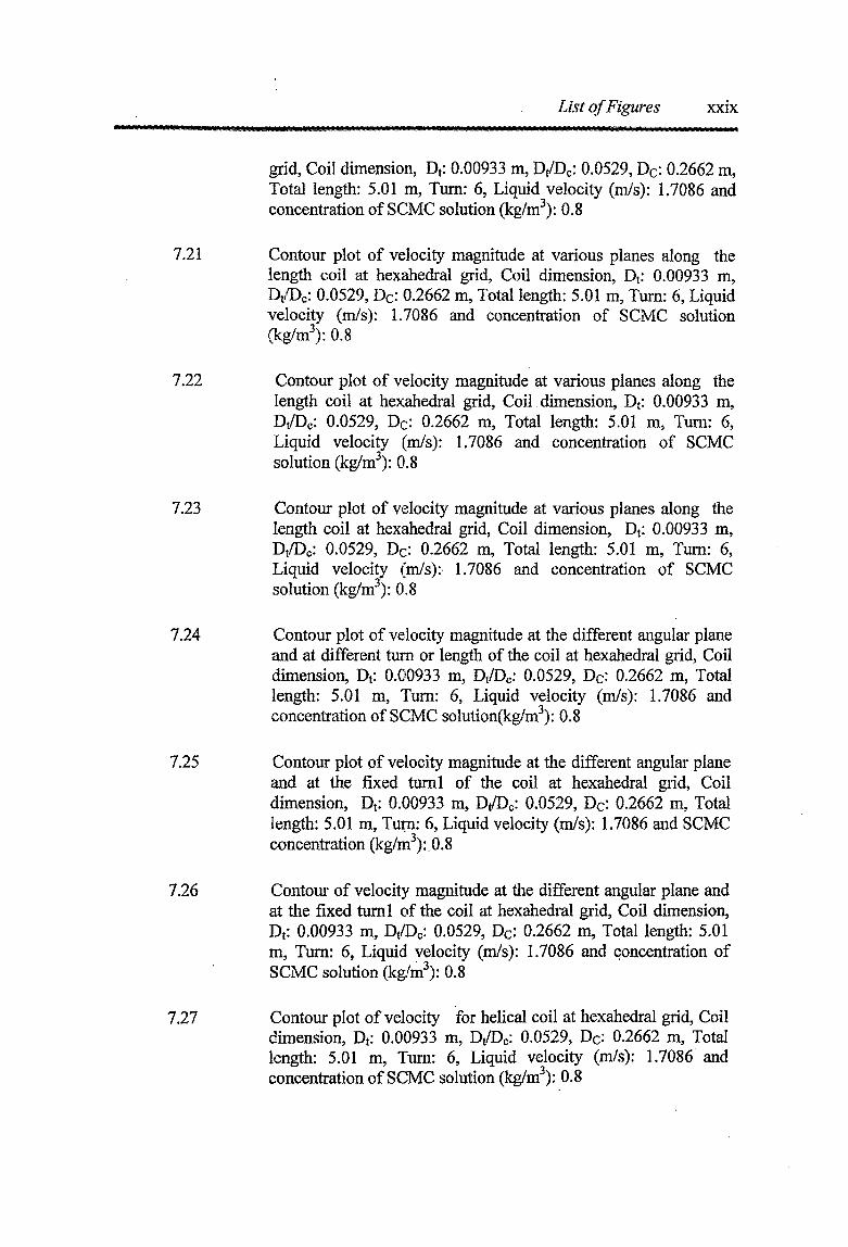
grid, Coil dimension, Dt: 0.00933 m, Dt/Dc: 0.0529, Dc: 0.2662 m, Total length: 5.01 m, Turn: 6, Liquid velocity (m/s): 1.7086 and concentration of SCMC solution (kg/m3): 0.8
Contour plot of velocity magnitude at various planes along the length coil at hexahedral grid, Coil dimension, Dt: 0.00933 m, Dt/Dc: 0.0529, Dc: 0.2662 m, Total length: 5.01 m, Turn: 6, Liquid velocity (m/s): 1.7086 and concentration of SCMC solution (kg/m3): 0.8
Contour plot of velocity magnitude at various planes along the length coil at hexahedral grid, Coil dimension, Dt: 0.00933 m, Dt/Dc: 0.0529, Dc: 0.2662 m, Total length: 5.01 m, Turn: 6, Liquid velocity (m/s): 1.7086 and concentration of SCMC solution (kg/m3): 0.8
Contour plot of velocity magnitude at various planes along the length coil at hexahedral grid, Coil dimension, Dt: 0.00933 m, Dt/D0: 0.0529, Dc: 0.2662 m, Total length: 5.01 m, Turn: 6, Liquid velocity (m/s): 1.7086 and concentration of SCMC solution (kg/m3): 0.8
Contour plot of velocity magnitude at the different angular plane and at different turn or length of the coil at hexahedral grid, Coil dimension, Dt: 0.00933 m, Dt/Dc: 0.0529, Dc: 0.2662 m, Total length: 5.01 m, Turn: 6, Liquid velocity (m/s): 1.7086 and concentration of SCMC solution(kg/m3): 0.8
Contour plot of velocity magnitude at the different angular plane and at the fixed tuml of the coil at hexahedral grid, Coil dimension, Dt: 0.00933 m, Dt/Dc: 0.0529, Dc: 0.2662 m, Total length: 5.01 m, Turn: 6, Liquid velocity (m/s): 1.7086 and SCMC concentration (kg/m3): 0.8
Contour of velocity magnitude at the different angular plane and at the fixed tuml of the coil at hexahedral grid, Coil dimension, Dt: 0.00933 m, Dt/Dc: 0.0529, Dc: 0.2662 m, Total length: 5.01 m, Turn: 6, Liquid velocity (m/s): 1.7086 and concentration of SCMC solution (kg/m3): 0.8
Contour plot of velocity for helical coil at hexahedral grid, Coil dimension, Dt: 0.00933 m, Dt/Dc: 0.0529, Dc: 0.2662 m, Total length: 5.01 m, Turn: 6, Liquid velocity (m/s): 1.7086 and concentration of SCMC solution (kg/m3): 0.8

List of Figures xxx
7.28 Contour plot of velocity at various planes along the length coil for helical coil at hexahedral grid, Coil dimension, Dt: 0.00933 m, Dt/Dc: 0.0529, Dc: 0.2662 m, Total length: 5.01 m, Turn: 6, Liquid velocity (m/s): 1.7086 and concentration of SCMC solution (kg/m3): 0.8
7.29 Contour plot of velocity at the different angular plane and at different turn or length of the coil at hexahedral grid, Coil dimension, Dt: 0.00933 m, Dt/Dc: 0.0529, Dc: 0.2662 m, Total length: 5.01 m, Turn: 6, Liquid velocity (m/s): 1.7086 and SCMC concentration (kg/m3): 0.8
7.30 Contour plot of velocity at the different angular plane and at different turn or length of the coil at hexahedral grid, Coil dimension, Dt: 0.00933 m, Dt/Dc: 0.0529, Dc: 0.2662 m, Total length: 5.01 m, Turn: 6, Liquid velocity (m/s): 1.7086 and concentration of SCMC solution (kg/m3): 0.8
7.31 Contour plot of velocity at the different angular plane and at the fixed tuml of the coil at hexahedral grid, Coil dimension, Dt: 0.00933 m, Dt/Dc: 0.0529, Dc: 0.2662 m, Total length: 5.01 m, Turn: 6, Liquid velocity (m/s): 1.7086 and concentration of SCMC solution (kg/m3): 0.8
7.32 Contour plot of velocity at the different angular plane and at the fixed tuml of the coil at hexahedral grid, Coil dimension, Dt: 0.00933 m, Dt/Dc: 0.0529, Dc: 0.2662 m, Total length: 5.01 m, Turn: 6, Liquid velocity (m/s): 1.7086 and concentration of SCMC solution (kg/m3): 0.8
7.33 Contour plot of velocity vector for helical coil at (a) hexahedral grid (b) tetrahedral grid, Coil dimension, Dt: 0.00933 m, Dt/Dc: 0.0529, Dc: 0.2662 m, Total length: 5.01 m, Turn: 6, Liquid velocity (m/s): 1.7086 and concentration of SCMC solution (kg/m3): 0.8
7.34 Contour plot of velocity vector at the different angular plane ofthe coil at hexahedral grid, Coil dimension, Dt: 0.00933 m, Dt/Dc: 0.0529, Dc: 0.2662 m, Total length: 5.01 m, Turn: 6, Liquid velocity (m/s): 1.7086 and concentration of SCMC solution (kg/m3): 0.8

List of Figures xxxi
7.35
7.36
7.37
7.38
7.39
7.40
7.41
7.42
7.43
Contour plot of velocity vector at the different angular plane and at different turn or length of the coil at hexahedral grid, Coil dimension, Dt: 0.00933 m, Dt/Dc: 0.0529, Dc: 0.2662 m, Total length: 5.01 m, Turn: 6, Liquid velocity (m/s): 1.7086 and concentration of SCMC solution (kg/m3): 0.8
Contour plot of velocity vector at the different angular plane and at the fixed tuml of the coil at hexahedral grid, Coil dimension, Dt: 0.00933 m, Dt/Dc: 0.0529, Dc: 0.2662 m. Total length: 5.01 m, Turn: 6, Liquid velocity (m/s): 1.7086 and concentration of SCMC solution (kg/m3): 0.8
Contour plot of helicity for helical coil at hexahedral grid, Coil dimension, Dt: 0.00933 m, Dt/Dc: 0.0529, Dc: 0.2662 m, Total length: 5.01 m, Turn: 6, Liquid velocity (m/s): 1.7086 and concentration of SCMC solution (kg/m3): 0.8
Contour plot of vorticity for helical coil at hexahedral grid, Coil dimension, Dt: 0.00933 m, Dt/Dc: 0.0529, Dc: 0.2662 m, Total length: 5.01 m, Turn: 6, Liquid velocity (m/s): 1.7086 and concentration of SCMC solution (kg/m3): 0.8
Contour plot of cell Reynolds number for helical coil at hexahedral grid, Coil dimension, Dt: 0.00933 m, Dt/Dc: 0.0529, Dc: 0.2662 m, Total length: 5.01 m, Turn: 6, Liquid velocity (m/s): 1.7086 and concentration of SCMC solution (kg/m3): 0.8
Contour plot of strain rate at hexahedral grid, Coil dimension, Dt: 0.00933 m, Dt/Dc: 0.0529, Dc: 0.2662 m, Total length: 5.01 m, Turn: 6, Liquid velocity (m/s): 1.7086 and concentration of SCMC (kg/m3) solution : 0.8
Contour plot of strain rate at the different angular plane along the length of the coil at hexahedral grid, Coil dimension, Dt: 0.00933 m, Dt/Dc: 0.0529, Dc: 0.2662 m, Total length: 5.01 m, Turn: 6, Liquid velocity (m/s): 1.7086 and concentration of SCMC solution (kg/m3): 0.8
Contour plot of shear stress for helical coil at hexahedral grid, Coil dimension, Dt: 0.00933 m, Dt/Dc: 0.0529, Dc: 0.2662 m, Total length: 5.01 m, Turn: 6, Liquid velocity (m/s): 1.7086 and concentration of SCMC solution (kg/m3): 0.8
Contour plot of shear stress at the different angular plane along

List of Figures xxxii
7.44
7.45
7.46
7.47
7.48
7.49
7.50
7.51
8.1
8.2
8.3
the length of the coil at hexahedral grid, Coil dimension, Dt: 0.00933 m, Dt/Dc: 0.0529, Dc: 0.2662 m, Total length: 5.01 m, Turn: 6, Liquid velocity (m/s): 1.7086 and concentration of SCMC solution (kg/m3): 0.8Comparison plot of helical coil at different SCMC concentration
Comparison plot of helical coil at different coil diameter
Comparison of present prediction with the experimental data (a) dimensionless shear stress (b) pressure drop
Development of axial velocity profile at different cross-sectional planes in curved tube at curvature ratio = 28, coil turn = 2, VL = 1.7086 m/s, SCMC conc.(kg/m3) = 0.8 in (a) horizontal centerline and (b) vertical centerline
Effect of liquid velocity on development of axial velocity profile in curved tube at curvature ratio = 28, coil turn = 2
Effect of coil turn or coil length, H on the development of axial velocity profile in (a) horizontal centerline (b) vertical centerline
Effect of curvature ratio on the development of axial velocity profile in (a) horizontal centerline (b) vertical centerline, Vl = 1.7086 m/s, SCMC conc.(kg/m3) = 0.8
Comparison plot of the experimental and calculated data for friction factor across the coil for different liquid (SCMC) concentration
Schematic diagram of helical coil
Contour plot of static pressure mixture at (a) hexahedral and (b) tetrahedral grid, Coil dimension, Dt: 0.00933 m, Dt/Dc: 0.0431, Dq: 0.2162 m, Total length: 6.10 m, Turn: 9, Concentration of SCMC solution: 0.8 kg/m3, Liquid velocity: 1.9531 m/s, Gas velocity: 0.7218 m/s, Gas Fraction, ag : 0.231
Contour plot of static pressure at (a) hexahedral and (b) tetrahedral grid, Coil dimension, Dt: 0.00933 m, Dt/Dc: 0.0350, Dc: 0.2662 m, Total length: 5.01 m, Turn: 6, Concentration of SCMC solution: 0.8 kg/m3, Liquid velocity: 1.7086 m/s, Gas
List of Figures xxxm
velocity: 0.9282 m/s, Gas fraction, ag : 0.3750
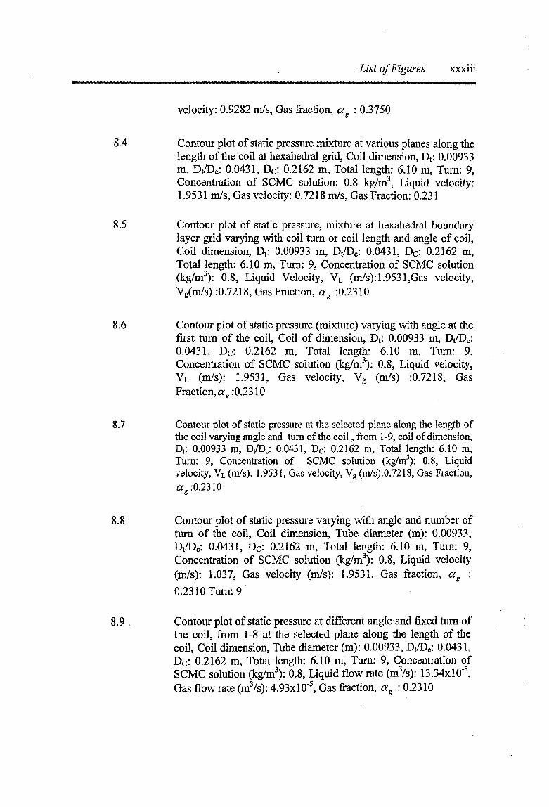
8.4 Contour plot of static pressure mixture at various planes along the length of the coil at hexahedral grid, Coil dimension, Dt: 0.00933 m, Dt/Dc: 0.0431, Dc: 0.2162 m, Total length: 6.10 m, Turn: 9, Concentration of SCMC solution: 0.8 kg/m3, Liquid velocity: 1.9531 m/s, Gas velocity: 0.7218 m/s, Gas Fraction: 0.231
8.5 Contour plot of static pressure, mixture at hexahedral boundary layer grid varying with coil turn or coil length and angle of coil, Coil dimension, Dt: 0.00933 m, Dt/Dc: 0.0431, Dc: 0.2162 m, Total length: 6.10 m, Turn: 9, Concentration of SCMC solution (kg/m3): 0.8, Liquid Velocity, Vl (m/s): 1.9531,Gas velocity, Vg(m/s) :0.7218, Gas Fraction, ag :0.2310
8.6 Contour plot of static pressure (mixture) varying with angle at the first turn of the coil, Coil of dimension, Dt: 0.00933 m, Dt/Dc: 0.0431, Dc: 0.2162 m, Total length: 6.10 m, Turn: 9, Concentration of SCMC solution (kg/m3): 0.8, Liquid velocity, Vl (m/s): 1.9531, Gas velocity, Vg (m/s) :0.7218, Gas Fraction, org:0.2310
8.7 Contour plot of static pressure at the selected plane along the length of the coil varying angle and turn of the coil, from 1-9, coil of dimension, Dt: 0.00933 m, Dt/Dc: 0.0431, Dc: 0.2162 m, Total length: 6.10 m, Turn: 9, Concentration of SCMC solution (kg/m3): 0.8, Liquid velocity, VL (m/s): 1.9531, Gas velocity, Vg (m/s):0.7218, Gas Fraction, ag: 0.2310
8.8 Contour plot of static pressure varying with angle and number of turn of the coil, Coil dimension, Tube diameter (m): 0.00933, Dt/Dc: 0.0431, Dc: 0.2162 m, Total length: 6.10 m, Turn: 9, Concentration of SCMC solution (kg/m3): 0.8, Liquid velocity (m/s): 1.037, Gas velocity (m/s): 1.9531, Gas fraction, ag :0.2310 Turn: 9
8.9 Contour plot of static pressure at different angle and fixed turn of the coil, from 1-8 at the selected plane along the length of the coil, Coil dimension, Tube diameter (m): 0.00933, Dt/Dc: 0.0431, Dc: 0.2162 m, Total length: 6.10 m, Turn: 9, Concentration of SCMC solution (kg/m3): 0.8, Liquid flow rate (m3/s): 13.34x1 O'5, Gas flowrate (m3/s): 4.93xl0'5, Gas fraction, ag : 0.2310

List of Figures xxxiv
8.10
8.11
8.12
8.13
8.14
8.15
Contours plot of total pressure varying with angle and coil height Coil dimension, Dt: 0.00933 m, Dt/Dc: 0.0350, Dc: 0.2662 m, Total length: 5.01 m, Turn: 6, Concentration of SCMC solution: 0.8 kg/m3, Liquid velocity: 1.7086 m/s, Gas velocity: 0.9282 m/s, Gas fraction, ag : 0.3750
Contours plot of total pressure (mixture) at the first turn of the coil varying with angle grid at the selected plane along the of the helical coil, Coil dimension, Dt: 0.00933 m, Dt/Dc: 0.0350, Dc: 0.2662 m, Total length: 5.01 m, Turn: 6, Concentration of SCMC solution: 0.8 kg/m3, Liquid velocity: 1.7086 m/s, Gas velocity: 0.9282 m/s, Gas fraction, ag : 0.3750
(a) Contours plot of velocity magnitude for mixture and (b) Contours plot of velocity magnitude at various planes along the length of the coil at hexahedral grid, Coil dimension, Dt: 0.00933 m, Dt/Dc: 0.0431, Dc: 0.2162 m, Total length: 6.10 m, Turn: 9, Concentration of SCMC solution : 0.8 kg/m3, Liquid velocity: 1.9531 m/s, Gas velocity: 0.7218 m/s, Gas fraction, ag: 0.231
Contour plot of velocity at the selected plane along the length of the coil varying with angle and turn of the coil from 1-9 , Coil dimension: Dt: 0.00933 m, Dt/Dc: 0.0431, Dc: 0.2162 m, Total length: 6.10 m, Turn: 9, Concentration of SCMC solution: 0.8kg/m3, Liquid velocity: 1.9531 m/s, Gas velocity: 0.7218 m/s, Gas fraction, ag: 0.231
Contour plot of velocity magnitude at the different angular plane and at any fixed turn of the coil, Coil dimension, Dt: 0.00933 m, Dt/Dc: 0.0350, Dc: 0.2662 m, Total length: 5.01 m, Turn: 6, Concentration of SCMC solution: 0.8 kg/m3, Liquid velocity: 1.7086 m/s, Gas velocity: 0.9282 m/s, Gas fraction, ag : 0.3750
(a) Contour plot of velocity magnitude for air phase at various planes along the length of the coil (b) Contours plot of velocity magnitude for air phase varying with angle and coil height, Coil dimension, Dt: 0.00933 m, Dt/Dc: 0.0350, Dc: 0.2662 m, Total length: 5.01 m, Turn: 6, Concentration of SCMC solution: 0.8 kg/m3, Liquid velocity: 1.7086 m/s, Gas velocity: 0.9282 m/s, Gas fraction, ag : 0.3750

List of Figures xxxv
8.16 Contours plot of velocity magnitude for air phase at the first turn of the coil varying with angle for hexahedral grid at the selected plane along the length of the coil, Coil dimension, Dt: 0.00933 m, Dt/Dc: 0.0350, Dc: 0.2662 m, Total length: 5.01 m, Turn: 6, Concentration of SCMC solution: 0.8 kg/m3, Liquid velocity: 1.7086 m/s, Gas velocity: 0.9282 m/s, Gas fraction, ag : 0.3750
8.17 (a) Contour plot of velocity magnitude for liquid phase at various planes along the length of the coil(b) Contours plot of velocity magnitude for liquid phase varying with angle and coil height at hexahedral grid, Coil dimension, Dt: 0.00933 m, Dt/Dc: 0.0350, Dc: 0.2662 m, Total length: 5.01 m, Turn: 6, Concentration of SCMC solution: 0.8 kg/m3, Liquid velocity: 1.7086 m/s, Gas velocity: 0.9282 m/s, Gas fraction, ag : 0.3750
8.18 Contours plot of velocity magnitude for liquid phase at the first turn of the coil varying with angle for hexahedral grid at the selected plane along the length of the coil, Coil dimension, Dt: 0.00933 m, Dt/Dc: 0.0350, Dc: 0.2662 m, Total length: 5.01 m, Turn: 6, Concentration of SCMC solution: 0.8 kg/m3, Liquid velocity: 1.7086 m/s, Gas velocity: 0.9282 m/s, Gas fraction, ag :0.3750
8.19 Contour plot of velocity vector at (a) hexahedral and (b) tetrahedral grid, Coil dimension, Dt: 0.00933 m, Dt/Dc: 0.0431, Dc: 0.2162 m, Total length: 6.10 m, Turn: 9, Concentration of SCMC solution: 0.8 kg/m3, Liquid velocity: 1.9531 m/s, Gas velocity: 0.7218 m/s, Gas fraction, ag : 0.231
8.20 Contour plot of velocity vector varying with angle and coil turn or height at hexahedral grid, Coil dimension, Dt: 0.00933 m, Dt/Dc: 0.0350, Dc: 0.2662 m, Total length: 5.01 m, Turn: 6, Concentration of SCMC solution: 0.8 kg/m3, Liquid velocity:l. 7086 m/s, Gas velocity: 0.9282 m/s, Gas fraction, ag : 0.3750
8.21 Contours plot of velocity vector at the first turn of the coil varying with angle for hexahedral grid at the selected plane of the coil, Coil dimension, Dt: 0.00933 m, Dt/Dc: 0.0350, Dc: 0.2662m, Total length: 5.01m, Turn: 6, Concentration of SCMC solution: 0.8kg/m3, Liquid velocity: 1.7086 m/s, Gas velocity: 0.9282 m/s, Gas fraction, ag : 0.3750

List of Figures xxxvi
8.22
8.23
8.24
8.25
8.26
8.27
8.28
Contour plot of velocity vector for liquid phase at hexahedral grid, Coil dimension, Dt: 0.00933m, Dt/Dc: 0.0529, Dc: 0.2662 m, Total length: 5.01 m, Turn: 6, Concentration of SCMC solution: 0.8 kg/m3, Liquid velocity: 1.7086 m/s, Gas velocity: 0.9282 m/s, Gas fraction, ag : 0.3750
Contour plot of velocity vector for liquid phase varying with angle and coil height at hexahedral grid, Coil dimension, Dt: 0.00933 m, Dt/Dc: 0.0350, Dc: 0.2662 m, Total length: 5.01 m, Turn: 6, Concentration of SCMC solution: 0.8 kg/m3, Liquid velocity: 1.7086 m/s, Gas velocity: 0.9282 m/s, Gas fraction, ag : 0.3750
Contour plot of velocity vector for liquid phase varying with angle and coil tuml at hexahedral grid at the selected plane of the coil, Coil dimension, Dt: 0.00933 m, Dt/Dc: 0.0350, Dc: 0.2662 m, Total length: 5.01 m, Turn: 6, Concentration of SCMC solution: 0.8 kg/m, Liquid velocity: 1.7086 m/s, Gas velocity: 0.9282 m/s, Gas fraction, ag : 0.3750
(a) Contour plot of velocity vector for air phase and (b) Velocity vector plot for air phase at various plane along the length of the coil at hexahedral grid, Coil dimension, Dt: 0.00933 m, Dt/Dc: 0.0529, Dc: 0.2662 m, Total length: 5.01 m, Turn: 6, Concentration of SCMC solution : 0.8 kg/m3, Liquid velocity:1.7086 m/s, Gas velocity: 0.9282 m/s, Gas fraction, ag : 0.3750
Contour plot of velocity vector for air phase varying with angle and coil height at hexahedral grid, Coil dimension, Dt: 0.00933 m, Dt/Dc: 0.0350, Dc: 0.2662 m, Total length: 5.01 m, Turn: 6, Concentration of SCMC solution: 0.8 kg/m3, Liquid velocity:1.7086 m/s, Gas velocity: 0.9282 m/s, Gas fraction, ag : 0.3750
Contours plot of velocity vector for air phase at the first turn of the coil varying with angle at hexahedral grid at the selected plane along the length of the coil, Coil dimension, Dt: 0.00933 m, Dt/Dc: 0.0350, Dc: 0.2662 m, Total length: 5.01 m, Turn: 6, Concentration of SCMC solution: 0.8 kg/m3, Liquid velocity:1.7086 m/s, Gas velocity: 0.9282 m/s, Gas fraction, ag: 0.3750
Contour plot of volume fraction at the selected plane for air-
List of Figures xxxvii
8.29
8.30
8.31
8.32
8.33
SCMC phase varying with angle and coil turn at hexahedral boundary layer grid, Coil dimension, Dt: 0.00933 m, Dt/Dc: 0.0431, Do' 0.2162 m, Total length: 6.10 m, Turn: 9, Concentration of SCMC solution (kg/m3): 0.8, Liquid velocity, Vl (m/s): 1.9531, Gas velocity, Vg (m/s):0.7218, Gas Fraction, a ‘0.2310
5
(a) Contours plot of volume fraction for liquid phase and (b) Contour plot of volume fraction for liquid phase at various planes along the length of the coil at hexahedral grid at the selected plane along the length of the coil, Coil dimension, Dt: 0.00933 m, Dt/Dc: 0.0350, Dc: 0.2662 m, Total length: 5.01 m, Turn: 6, Concentration of SCMC solution: 0.8 kg/m3, Liquid velocity: 1.7086 m/s, Gas velocity: 0.9282 m/s, Gas fraction, ag : 0.3750
Contours plot of volume fraction for liquid phase at the first turn of the coil varying with angle at hexahedral grid at the selected plane along the length of the coil, Coil dimension, Dt: 0.00933 m, Dt/Dc: 0.0350, Dc: 0.2662 m, Total length: 5.01 m, Turn: 6, Concentration of SCMC solution: 0.8 kg/m3, Liquid velocity: 1.7086 m/s, Gas velocity: 0.9282 m/s, Gas fraction, ag : 0.3750
Contours plot of volume fraction for liquid phase varying with angle and coil height at hexahedral grid, Coil dimension, Dt: 0.00933 m, Dt/Dc: 0.0350, Dc: 0.2662 m, Total length: 5.01 m, Turn: 6, Concentration of SCMC solution: 0.8 kg/m3, Liquid velocity: 1.7086 m/s, Gas velocity: 0.9282 m/s, Gas fraction, ag:0.3750,
(a) Contour plot of volume fraction for air phase (b) Contours of volume fraction for air phase at various planes along the length of the coil at hexahedral grid, Coil dimension, Dt: 0.00933 m, Dt/Dc: 0.0431, Dc: 0.2162 m, Total length: 6.10 m, Turn: 9, Concentration of SCMC solution: 0.8 kg/m3. Liquid velocity: 1.9531 m/s, Gas velocity: 0.7218 m/s, Gas fraction, ag : 0.231
Contour plot of volume fraction for air phase at the first turn of the coil varying with angle at hexahedral grid at the selected plane along the length of the helical coil, Coil dimension, Dt: 0.00933 m, Dt/Dc: 0.0529, Dc: 0.2662 m, Total length: 5.01 m, Turn: 6, Concentration of SCMC solution: 0.8 kg/m3, Liquid velocity: 1.7086 m/s, Gas velocity: 0.9282 m/s, Gas fraction, ag:

List of Figures xxxviii
0.3520
8. 34 Contours plot of volume fraction for air phase varying with angleand coil height grid, Coil dimension, Dt: 0.00933 m, Dt/Dc: 0.0350, Dc: 0.2662 m, Total length: 5.01 m, Turn: 6, Concentration of SCMC solution: 0.8 kg/m3, Liquid velocity: 1.7086 m/s, Gas velocity: 0.9282 m/s, Gas fraction, ag: 0.3750
8.35 Path lines of particle ID mixture
8.36 Comparison plot for helical coil
8.37 Comparison plot for helical coil at different SCMC concentration
8.38 Comparison plot of experimental data and CFD analysis for helical coil for two-phase frictional pressure drop per unit length of the coil with gas flow rate at constant liquid flow rate and constant SCMC solution for different coil diameter
8.39 Comparison of present prediction with the experimental data: (a) pressure drop (b) void fraction
8.40 Effect of gas and liquid velocity on liquid volume fraction in curved tube at curvature ratio =18, coil turn = 2
8.41 Effect of gas and liquid velocity on development of axial velocity profile in curved tube at curvature ratio 18, coil turn = 2, Vl=1.9531 m/s, in horizontal centerline
8.42 Effect of coil turns or coil length on the development of axial velocity profile in (a) horizontal centerline and (b) vertical centerline
8.43 Effect of angle on the development of axial velocity profile in (a) horizontal centerline and (b) vertical centerline
8.44 Effect of curvature ratio on the development of axial velocity profile in (a) horizontal centerline and (b) vertical centerline, at VG = 0.8433 m/s, VL = 1.9531 m/s

Synopsis
SYNOPSIS
The hydrodynamics of single and two-phase gas-liquid flow have received
extensive treatment during few decades because of their widespread application in
industry. It occurs in boiler tubes, distillation columns, oil and gas wells, transportation
system of crudes and refined products, all key pieces of equipment in refineries,
petrochemical industries, polymer processing, nuclear engineering and large number of
chemical reactor applications. With the development in polymer processing, mineral
recovery, food processing, biomedical engineering, biochemical engineering, gas-liquid-
solid reactions, hydraulic transportation the liquids most often be non-Newtonian in
nature. Hence, there is a need to study the flow of non-Newtonian and gas-non-
Newtonian liquid flow through piping components and helical coils.
The computational fluid dynamics (CFD) is a powerful tool to evaluate the
frictional losses and estimate the other flow characteristics can be visualized to aid in
better understanding of the flow phenomenon and it can be applied to improve flow
characteristics and equipment design. However, the simulation models are generally
empirical in nature and caution must be exercised in their application to practical cases
which may involve detailed investigation of all the involved assumptions and limitations.
Such modeling would always require fine tuning by comparison with reliable
experimental data.
Thus in view of the importance of the single-phase and two-phase gas-liquid flow
through piping components and helical coils, and the CFD simulation using a commercial
software Fluent 6.3, a research programme has been undertaken in investigate the
following aspects,

Synopsis xl
1. Experimental studies and CFD analysis for water and air-water flow through U -
bends,
2. Experimental studies and CFD simulation on the non-Newtonian fluid flow
through piping components,
3. CFD analysis on the gas-non-Newtonian liquid flow through piping components,
4. Experimental studies and CFD analysis on the non-Newtonian liquid flow through
helical coils,
5. CFD simulation on the Gas- non-Newtonian liquid flow through helical coils.
The thesis has been presented in the eight chapters :
Chapter - 1 : It presents an overview and importance of the existing information in the
flow of liquid and gas-liquid flow through piping components and helical coils. The
importance of the computational Fluid Dynamics (CFD) is also highlighted.
Chapter - 2 : It describes the CFD methodology used for the simulation.
Chapter - 3 : It consists of the experimental studies on the pressure loss for water and
air-water flow through four different U-bends of different radius of curvatures. The range
of flow rate used for air and water in the experiments are 5.936 x 10'5 - 56.1189 x 10‘5
m3/s and 2.000 x 10"4- 4.6500 x 1 O'4 m3/s respectively. The CFD simulations are carried
out using k-s model and standard mixture k-s model for water and air-water flow through
U-bends. The simulated result gives the detail flow phenomena inside the U-bends for
water and air-water flow. The CFD simulated pressure drop agrees well the experimental
data.
Chapter — 4 : It consists of experimental studies on the non-Newtonian liqui flow
through piping components. Dilute aqueous solutions of Sodium salt of carboxymethyl

Synopsis xli
cellulose (SCMC) is used as non-Newtonian liquids. Piping components used for the
experiment are elbows of three different angles, orifices, gate valves and globe valves.
The flow rates used for the experiment are 3.75x1 O'5 - 29.83x1 O'5 m3/s. Empirical
correlations have been developed to predict the pressure losses across the piping
components.
Chapter - 5 : It consists of the CFD analysis of non-Newtonian liquid flow through
piping components. Single phase laminar non-Newtonian power law model is used for
the simulation. The CFD analysis gives the insight of the flow phenomena of the piping
components. The CFD simulated pressure drop data matches well with the experimental
data.
Chapter - 6 : It consists of the CFD analysis on two-phase gas-non-Newtonian liquid
flow through piping components. Laminar non-Newtonian power law Eulerian
multiphase model have been used for simulation. The simulated results gives the insight
flow phenomena, velocity magnitude, velocity vector, static pressure, volume fraction of
different phases. The simulated two-phase pressure drop data matches well with our
earlier published experimental data.
Chapter - 7 : It consists of the experiment and CFD analysis of non-Newtonian liquid
flow through helical coils. Dilute aqueous solution of sodium salt of carboxymethyl
cellulose (SCMC) used as non-Newtonian liquids. The range of liquid flow rates used for
the experiments is 3.334xl0'5 - 15.003xl0"5 m3/s. Single phase laminar non-Newtonian
power law model is used for the CFD simulation. The CFD simulation gives the insight
of velocity and pressure field of the coil. The CFD simulated results matches well with

Synopsis xlii
the experimental results. The experimental and CFD simulated results are compare with
the other values obtained from literature.
Chapter - 8 : It consists of the CFD analysis of gas-non-Newtonian liquid flow through
helical coils. Laminar non-Newtonian power law Eulerian multiphase model have been
used for CFD simulation. The simulation gives the insight flow phenomena of velocity
magnitude, velocity vector, static pressure, volume fraction of the different phases. The
two-phase CFD simulated pressure drop data matches well with the experimental data
obtained earlier in our laboratory. It is also noted that simulated data at hexahedral grid
gives the better result than tetrahedral grid.

Chapter 1
Introduction

Chapter 1 Introduction 2
The hydrodynamics of single-phase and gas-liquid two-phase flows have received
extensive treatment during last few decades because of their widespread application in
industry. This chapter deals with the importance of the hydrodynamics studies and the
computational Fluid Dynamics (CFD). Here the literature review attempted is not breadth
or depth of coverage but is focused mainly on the importance of the flow studies.
1.1 Introduction
Pipe fittings such as elbows, bends, valves, orifices are integral part of any piping
system. The flow in fittings is considerably more complex than in a straight pipe. The
problem of determining the pressure losses in pipe fittings is important in design and
analysis of the fluid machinery. Forcing a fluid through pipe fittings consumes energy
detected by the drop in pressure across the fittings. The friction between the fluid and the
fitting wall causes this pressure drop. The problem of predicting pressure losses in pipe
fittings is much more uncertain than for the pipe because,
i. The mechanism of flow is not clearly defined. At least two types of losses are
superposed – skin friction and the loss due to change in flow direction, and
ii. There are very few experimental data available in the literature.
Two–phase flow through pipe fittings are even much more complex than that of
straight pipes and only few experimental data are available in literature (Mandal and Das,
2003). When fluid flows through a curved pipe, it generates secondary flows due to the
interaction between centrifugal and viscous forces. The secondary flow fields become
more complex due to the combined effects of the coriolis force (due to torsion of the tube
centerline) and the centrifugal force (due to the curvature), i.e., simultaneous effect of
curvature and torsion on the flow. When two-phase flow enters the curved portion, the
Chapter 1 Introduction 3
heavier density phase is subjected to a large centrifugal force, which causes the liquid to
move away from the centre of curvature, whereas the gas flows towards the center of the
curvature. Separation of phases in this way is likely to give rise to significant slip
between the phases. This process is a continuous function of the coil geometry. Despite
various applications, the literature on two-phase flow through coiled tubes is rather
meager (Biswas, 2008).
Fluid flows play the key roles in the working process of many modern
engineering devices. Designing of these devices for the required operational parameters is
impossible without reliable prediction of characteristics of these flows. As many
engineering devices are very expensive and labour intensive in their manufacturing
process, so their physical modeling with experimental determination of their working
parameters at different possible models, as a rule, requires large temporal and financial
expenses. Besides, due to restricted possibilities of modern experimental sensors and
measuring instruments, experimental observations do not give complete information
about the investigated phenomena. Due to the nature of fluid medium itself, fluid flows
often occur in very complex manner, with the presence of transitional effects, stagnation
zones, vortex structures, and at supersonic velocities – their possibilities of generation of
compression shock waves. The situation is still very complex when heat and mass
transfer is present, when considering flow of a mixture of gas-liquid, liquid-liquid, slurry
etc., free surface flows, flows with cavitation, boiling, condensation, combustion,
chemical reaction etc. are present. All these factors explain the growing interest for the
software tools for simulation of fluid flow allowing for the prediction of characteristics of
these flows and the working parameters of engineering devices at the stage of designing,

Chapter 1 Introduction 4
before the manufacturing. The branch of science dealing with simulation of fluid flows
with heat and mass transfer in various engineering and natural objects is computational
fluid dynamics (CFD).
The computational power of computers grew and at the same time, their prices
become reduce and affordable for more and more users, since the 70s of XX century,
rapid development of commercial CFD software has started. Till the beginning of 90s the
cheap personal computers have become as powerful as those of workstations, and CFD
software packages designed for PC have started.
Today dozens of software packages intended for solution of fluid flow problems
are available. A complete list is given at the site www.cfd-online.com. Among the CFD
software most recognized worldwide are Fluent, CFX, STAR-CD, Numeca etc. Initially
computational fluid dynamics was developed for solution of problems of aerospace
industry – simulation of processes in combustion chambers of rocket engines, simulation
of phesico-chemical processes in the flow around rocket airframe and supersonic
aircrafts. Today the field of application of CFD is essentially extended in all fields of
engineering where fluid flows occur.
In the field of chemical engineering the design of process equipment involves
specifying the configuration of the equipment and its operating protocols, which must be
acceptable in safety, environment and economic point of view. A wide variety of process
equipment and operating protocols/codes are used in practice. The major driving force of
these different designs are energy efficient and more control of the reactants, the process
and the easy removal of the products. In chemical or physical transformation process
requires the addition or removal of different materials and energy in right place and also

Chapter 1 Introduction 5
in right time. This can be achieved by controlling basic fluid dynamics. So the
understanding of the process and its requirements and identification of the actual or
desired fluid dynamic characteristics is essential. The CFD models are expected to help
in this direction.
Design engineers use CFD models for two purposes; “design” models, which
attempt to provide a quantitative relationship between the hardware and performance, and
“learning” models, which provide a basic understanding of different underlying processes
(Joshi and Ranade, 2003). With the help of CFD designer could predict what could or
would happen as a result of a specific design, thereby steering the design in promising
directions. It also help to end up with a new design concepts which often get sidelined
due to lack of resources like experimental facilities, time, funding etc. to test them.
The Vision 2020 document for the U. S. chemical industry
(http://www.chemicalvision2020.org/pdfs/compfluid.pdf) entitled Technology roadmap
for CFD identified the following performance targets for CFD,
i. Shorten the lead times (from research to final plant design) to 3-5 years.
ii. Reduce plant downtimes to 1%.
iii. Reduce the separation energy and improve the separation efficiency by
20%.
iv. Increase the reliability of the design (reduce risk).
v. Reduce/eliminate design errors.
vi. Promote innovation.
vii. Reduce fuel consumption per unit of product.
viii. Improve heat transfer (waste heat recovery).

Chapter 1 Introduction 6
ix. Optimize processes to increase yield and aid incremental expansion.
According to Joshi and Ranade (2003) this document is justified for the fulfillment of the
target because of the advancement in numerical methods and computers help to minimize
the errors due to numerical inaccuracies.
So basically computational fluid dynamics (CFD) is the science of predicting
fluid flow, heat and mass transfer, chemical reactions and related phenomena by solving
numerically the set of governing mathematical equations (conservation of mass,
momentum, energy). The results of CFD analysis are used for studies of new design,
product development, trouble shooting and redesign. CFD analysis complements testing
and experiments, reduces the total effort required in the experiment design and data
acquisition. Hence, the CFD analysis gives substantial reduction of times and costs of
new designs (Ranade, 2002).
A commercial fluent 6.3 solver is used to solve the basic governing mathematical
equation numerically based on the finite volume method in the present analysis presented
in the thesis. Geometries are created in Gambit 6.3 preprocessor. Geometries are
imported into Fluent 6.2/6.3 in a cartesian co-ordinate system. Fluent 6.2/6.3 solved the
governing equations in 3-D geometry. The use of CFD yields a very detailed solution
containing the local values of relevant variables, such as pressure, velocity, temperature,
viscosity, shear stress and so on.
1.2 Objective of the present work
Few experiments are conducted and other experimental data collected from past
Ph. D. thesis worked in our laboratory used for the present CFD analysis,
Chapter 1 Introduction 7
1. Experimental studies and CFD analysis for water and air–water flow through U–
bends.
2. Experimental studies and CFD simulation on the non-Newtonian fluid flow
through piping components,
3. CFD analysis on the gas-non-Newtonian liquid flow through piping components,
4. Experimental studies and CFD analysis on the non-Newtonian liquid flow through
helical coils,
5. CFD simulation on the Gas- non–Newtonian liquid flow through helical coils.

Chapter 2
CFD methodology
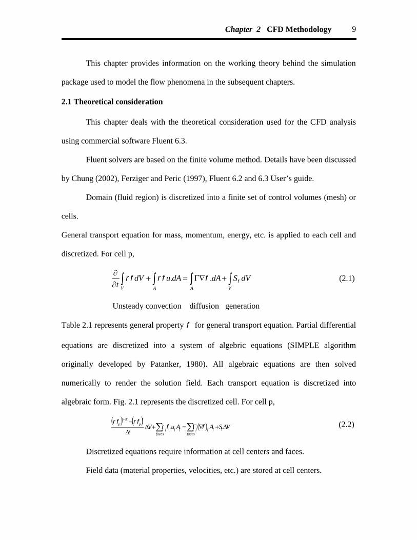
Chapter 2 CFD Methodology 9
This chapter provides information on the working theory behind the simulation
package used to model the flow phenomena in the subsequent chapters.
2.1 Theoretical consideration
This chapter deals with the theoretical consideration used for the CFD analysis
using commercial software Fluent 6.3.
Fluent solvers are based on the finite volume method. Details have been discussed
by Chung (2002), Ferziger and Peric (1997), Fluent 6.2 and 6.3 User’s guide.
Domain (fluid region) is discretized into a finite set of control volumes (mesh) or
cells.
General transport equation for mass, momentum, energy, etc. is applied to each cell and
discretized. For cell p,
dVSdAdAudVt VAAV
.. (2.1)
Unsteady convection diffusion generation
Table 2.1 represents general property for general transport equation. Partial differential
equations are discretized into a system of algebric equations (SIMPLE algorithm
originally developed by Patanker, 1980). All algebraic equations are then solved
numerically to render the solution field. Each transport equation is discretized into
algebraic form. Fig. 2.1 represents the discretized cell. For cell p,
facesffffff
facesf
tp
ttp VSAAuV
t
(2.2)
Discretized equations require information at cell centers and faces.
Field data (material properties, velocities, etc.) are stored at cell centers.

Chapter 2 CFD Methodology 10
Face values are interpolated in terms of local and adjacent cell values.
Discretization accuracy depends upon ‘stencil’ size.
The discretized equation can be expressed simply as:
pnbnb
nbpp baa (2.3)
Equation is written out for every control volume in domain resulting in equation set.
2.2 Mathematical model
2.2.1 Single phase water flow
Conservation of mass:
0. u (2.4)
where u is velocity vector.
Conservation of momentum:
Bupuuu Teffeff ... (2.5)
where B is a body force, p is the pressure, and T stands for transpose.
High Reynolds number k- turbulence model:
teff and
2kCt (2.6)
The transport equations for the turbulent kinetic energy ( k ) and turbulent
dissipation ( ) are
kuuuuukuk eff
T
effk
t ..3
2... (2.7)
21 ..3
2... Ckuuuuu
kCu eff
Teff
t
(2.8)

Chapter 2 CFD Methodology 11
Table 2.1 represents the empirical constants in k- turbulence model.
2.2.2 Mathematical Model for Air–water system
Governing equations and numerical methods
Standard k– turbulence model is used for single–phase water flow and mixture
standard k– multiphase model equations are used for two–phase air–water flow through
U–bends.
This approach allows for simulation of multi–phase flows when the substances of
different phases can intermix and do not form the free surface. In order to simulate the
flow of two or several phases, this model uses one continuity equation, one set of
momentum equations and one energy equation that are written with regard to mass–
averaged velocity and density of the mixture. Thus continuity equation in this model
looks as follows,
Solves one equation for Continuity of the mixture,
mut mmm
. (2.9)
Solves for the transport of volume fraction of each secondary phase
/.. kkkmkkkk uut
(2.10)
This model uses the conception of drift velocities to take account that motion of
different phases occurs with different velocities. This allows for simulation.
Solves one equation for the momentum of the mixture
n
kkkkkmmmmmmmm uuFguupuuu
t 1
/// ... (2.11)
Drift velocity mkk uuu /

Chapter 2 CFD Methodology 12
Where mixture properties are defined as
k
n
kkm
1
k
n
kkm
1 m
n
kkkk
m
uu
1 (2.12)
The standard k belong to high-Reynolds number models, which are primarily valid
for turbulent core flow while they neglect the effects of viscosity in the near-wall region.
These models necessitate the use of a wall function or a two-phase zonal approach.
2.3 Mathematical Model
2.3.1 Single phase non-Newtonian fluid
Governing equations and numerical methods
Dilute solution of SCMC follows the laminar non-Newtonian pseudo plastic
Power law model. In general for non-Newtonian liquids the effective viscosity is used for
calculation and defined as,
1/
/
8
n
eff d
uK (2.13)
The governing equation is the Navier – Stokes equation as,
Puuut
ueff
2. (2.14)
and the continuity equation is
0u (2.15)
where,z
ky
jx
i
(2.16)
2.3.2 For air-non-Newtonian fluid system
Eulerian multiphase model equations
Volume fraction equation

Chapter 2 CFD Methodology 13
The volume of phase q is defined as
q q
v
V dV (2.17)
Where q is volume fraction of phase q, and
1
1n
(2.18)
where n is number of phases.
Eulerian multiphase model equations
Two-phase flow was modeled with the Eulerian-Eulerian approach, where the
phases are assumed to be interpenetrating continua. One of the phases defined as
continuous and the other as dispersed, the phases sum up to the unity. The pressure and
gravity vectors are shared by both phases, whereas other variables are phase specific. The
only notable change to the one phase solution is the presence of interfacial forces.
This model is the most general and the most complex among all the models of
multi–phase flow. The substance of each phase is assumed to form continuous medium.
Its motion is simulated with own system of Navier–Stokes equations, continuity equation
and energy equation. According to this model, the equations written for each phase are
solved jointly. At high values of g , the dispersed particles strongly influence the carrier
flow, and only the multi–phase Eulerian model should be used for adequate simulation of
such flows.
Continuity
1.
n
q q q q q pqpu m
t
Where q = fraction for the q-th phase (2.19)
Momentum for q-th phase

Chapter 2 CFD Methodology 14
, ,1
. .n
q q q q q q q q q q q pq pq q q q q lift q vm qp
u u u p g R m u F F Ft
Transient convective pressure body shear interphase external, lift, and
Forces and mass virtual mass forces
Exchange
(2.20)
The inter-phase exchange forces are expressed as
pq pq p q pqR K u u whereK fluid fluidexchangecoefficient (2.21)
As the flow of liquid is laminar, non-Newtonian Power Law model is used as viscous
model and Eulerian model is used as multiphase model for the CFD analysis.
Where pu is the velocity of phase p, and pqK is the interphase momentum exchange
coefficient which can be written in the following general form:
q q qpq
p
fK
(2.22)
where p the volume fraction of phase p is, p is the density of phase p, f is the drag
function, and p is the particulate relaxation time which is defined as:
2
18p p
pp
d
(2.23)
where, pd is the diameter of the bubbles of phase p, and p is the viscosity of phase p.
The drag function, f , can be expressed as ( Schiller and Naumann, 1935),
Re
24DC
f (2.24)
where

Chapter 2 CFD Methodology 15
0.65724 1 0.15 Re / Re Re 1000DC
= 0.44 Re 1000 (2.25)
Where DC the drag coefficient and Re is is the relative Reynolds number which can be
obtained from:
q
pqpq duu
Re (2.26)
And q is the viscosity of phase q.
2.3.3 Estimation of the mesh cell size adjacent to the wall
The distance from the wall to the centroid of the first mesh cell ( y ) can be
estimated by choosing a desired y+ (ideally, y+=1) with the estimated bulk Reynolds
number as (ANSYS Fluent Inc., 2008).
11/7Re06.5
bhdy
y(2.27)
where y+ is a dimensionless number, hd is the hydraulic diameter, and bRe is the bulk
Reynolds number. These equations are solved subject to the following boundary
conditions,
(i) The piping components and coil walls are assumed rigid and a no-slip
condition is imposed.
(ii) At the outlet, the velocities are free but the normal and tangential stresses are
constrained to be zero and the gauge pressure is set to zero.
(iii) At the inlet, a uniform velocity profile is used with a time varying forcing
function representive of flow in the left portion of the bend.

Chapter 2 CFD Methodology 16
A three-dimensional computational grid was generated for each geometry studied
using the package GAMBIT 6.3. The geometry was drawn using Gambit. An
unstructured tetrahedral and boundary layer hexahedral mesh with nearly 5x10³- 20x 104
were used. Inlet and outlet are located at each end of the system. The inlet is used to
specify the inlet velocity and outlet is used to specify pressure outlet. The commercially
available CFD code, FLUENT Version 6.3, which is based on the finite-volume method,
was used.
Geometries are imported into FLUENT 6.3 in a Cartesian coordinate system. In
the simulation, the governing equations are solved for a full 3-D geometry. For flow
phenomena associated with single-phase non-Newtonian, water and two-phase air-non-
Newtonian, air - water flow, we have chosen laminar non-Newtonian power law model
for single-phase non-Newtonian and K-epsilon model for single-phase water flow. For
two-phase air-water flow we have choosen k-epsilon mixture model and two-phase air-
non-Newtonian flow we have choosen laminar Eulerian model. The model solves for
momentum equation and prescribes relative velocities to describe the dispersed phases.
Continuity equations for the gas phase coupled with a single continuity equation for the
liquid phase. In addition simulations were carried out with constant bubble size of 1mm
using mixture k and Eulerian model. The governing equations are non linear and
several iterations of loop must be performed before a convergent solution is obtained.
These equations solved sequentially by Segregated Solver. The standard k model is
used to solve the air-water flow and Eulerian model to solve air-non-Newtonian flow.
The first-order upwind scheme is used in the discretization of set of governing equations.

Chapter 2 CFD Methodology 17
Since there is significant difference in the velocities of two phases, slip velocity is turned
on in mixture parameters.
2.4 Numerical approach
The governing equations for the multiphase flow in piping components and coils
will be solved by the Eulerian–Eulerian approach. This approach treats different phases
as interpenetrating continua, and solves the momentum and continuity equations for each
phase individually. The phase coupling is achieved through the pressure and interphase
exchange coefficients.
2.4.1 CFD procedure
A general procedure to simulate gas mixing in piping components and coils based on
Gambit 6.3 and Fluent 6.3 software (ANSYS Fluent Inc., 2008) is outlined below,
i. Perform meshing under Gambit 6.3 - Create a computational domain at the flow
region, using tetrahedral and boundary layer hexahedral meshes where possible to
generate grids, and controlling a smooth change in the mesh size by size functions.
The boundary and continuum types should be specified. Examine the mesh to ensure
that the high skewness is below 0.5.
ii. Import the mesh file to Fluent 6.3 and check the mesh.
iii. Define a 3-D, unsteady, implicit, and pressure-based solver.
iv. Activate the Eulerian multiphase model.
1. Define a standard k- model including slip velocity.
2. Enable the water properties with turbulent flow conditions and non-Newtonian
fluid properties with laminar flow conditions using the text command:
define/models/viscous/turbulence

Chapter 2 CFD Methodology 18
3. Define the phases by setting water (or a non-Newtonian fluid) as the primary
phase and gas as the secondary phase, and keeping the default selection of
Schiller-Naumann drag model in the phase interaction panel.
4. Define the operating conditions by turning on gravity and specify the operating
density.
5. Define the boundary conditions.
Solution control methodology-Under-relaxation factors - 0.3 for pressure, 0.3 for
momentum, 0.1-0.9 for volume fraction, and default values for the other
parameters. Discretization schemes - standard for pressure, momentum and
volume fraction, and first-order upwind for other variables: momentum, turbulent
kinetic energy, turbulent dissipation rate. Easiest to converge, only first–order
accurate.
6. Pressure-velocity SIMPLE coupling used.
7. Initialize the solution–velocity.
8. Enable the plotting of residuals during the calculation, and keep the default
convergence criteria (10-5 for energy and 10-3 for continuity).
9. Enable a volume monitor for the volume-weighted average velocity of liquid
phase.
10. Set the time step size that can be estimated as a ratio of mesh cell size and gas
inlet velocity, and run a simulation until achieving a steady-state solution.
Chapter 2 CFD Methodology 19
2.4.2 Solver
The segregated (implicit) solver is preferred in all other cases, due to lower
memory requirements than coupled implicit solver. Segregated approach provides
flexibility in solution procedure
2.4.3 Convergence
All discrete conservation equations (momentum, energy, etc.) are obeyed in all
cells to a specified tolerance.
Solution no longer changes with more iteration.
Overall mass, momentum, energy, and scalar balances are achieved.
Monitoring convergence with residuals history:
Generally, a decrease in residuals by 3 orders of magnitude indicates at least
qualitative convergence.
Major flow features established.
Scaled energy residual must decrease to 10-6 for segregated solver.
Scaled species residual may need to decrease 10-5 to achieve species balance.
2.5 Conclusion
Basic fundamentals of CFD are discussed in this chapter.
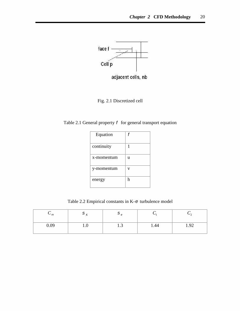
Chapter 2 CFD Methodology 20
Fig. 2.1 Discretized cell
Table 2.1 General property for general transport equation
Equation
continuity 1
x-momentum u
y-momentum v
energy h
Table 2.2 Empirical constants in K- turbulence model
C K 1C 2C
0.09 1.0 1.3 1.44 1.92

Chapter 3
Water and air-water flow through U-bends
Chapter 3 Water and Air-Water flow through U-bends 22
Experimental investigation has been carried out in order to study the water and
air-water flow through four different U-bends. Numerical modeling is carried using
Fluent 6.3 software to find its applicability.
3.1 Introduction
Bends are an integral part of any pipeline transport processes, and the flow
patterns developed are more complex than those of straight tubes. Fluid motion in a bend
is not parallel to the curved axis of the bend. When fluid flows through a curved pipe, the
presence of curvature generates a centrifugal force that acts right angles to the main flow,
resulting in secondary flow. The strength of secondary flow depends on the curvature of
the surface, i.e., radius of curvature of the bend. Information on flows in curved pipes is
highly important for many engineering applications in connection with confined curved
flows through bends, headers, cooling ducts and blade passages of turbines. Lack of
information, however, exists in spite of a lot of investigations which have been made by
many researchers.
Thomson (1876) first observed the curvature effects of bends on flows. Eustice
(1910) also observed the existence of secondary flows by injecting ink into water passing
through a coiled pipe. Wilson et al. (1922) observed that the pressure drop is dependent
on the flow Reynolds number and Dean (1928 a, b) studied the stability of a curved pipe
flow and identified the condition for the onset of secondary vortices. Ito (1959) indicated
that secondary flows can cause a rapid rise in friction and lead to a much increased
pressure drop. Tunstall and Harvey (1968) observed the presence of a main or primary
flow recirculation at the inner wall for tight bends (δ < 3). Berger et al. (1983) and Das
(1996) have provided a comprehensive review of literature on flows through curved
Chapter 3 Water and Air-Water flow through U-bends 23
pipes. The intensity of such secondary flows depends on the combination of the main
flow Reynolds number (Re) and the curvature ratio (δ=Rb/Rt) and can be characterized by
the dimensionless number called the Dean Number.
Enayet et al. (1982) measured, in a range of Reynolds numbers, Re, 500 to
4.6X10⁶, longitudinal components of mean and fluctuating velocities for the turbulent
water flow in a circular 90° bend using laser Doppler velocimeter. Azzola et al. (1986)
reported the computations method using the standard k—ε model and measurements of
developed turbulent flow in a 180° bend. Anwer et al. (1989) measured mean velocities
and Reynolds stresses in the horizontal and a normal plane in an 180o bend using hot wire
anemometer. Bend flows have been extensively studied experimentally by Kim and
Simon (1988), Al-Rafai et al. (1990), Cheng and Farokhi (1992), Anwer and So (1993),
Sudo et al. (1998) and Sudo et al. (2000).
The Computer simulations provide an efficient approach for studying flows
through curved pipes under various conditions. Practical simulations can also be
performed by solving the filtered Navier-Stokes equation using a Large-Eddy Simulation
(LES) or by solving the Reynolds Average Navier-Stokes (RANS) equation with an
appropriate closure model for the Reynolds stress (Pui et al., 1987; Van de Vosse et al.,
1989; Jayanti et al., 1990; Brockmann, 1993; Bergstrom et al., 1998; Wang and Shirazi,
2001; Breuer et al., 2006; Berrouk and Laurence, 2008; and Zhang et al., 2009, 2010,
etc.).
Two phase flow has got an enormous application in industry starting from
reboiler, Nuclear reactor to pipeline transportation, chemical, petrochemical, petroleum
refineries, and pharmaceutical industries. The need for reliable design methods has been

Chapter 3 Water and Air-Water flow through U-bends 24
the driving force behind a very large effort in two-phase gas-liquid flow over past few
decades. When a fluid flows through a bend the presence of curvature generates a
centrifugal force across the bend that acts right angle to main flow and results in
secondary flow. The strength of the secondary flow depends on the curvature of the
surface. This results in a pressure gradient between maximum pressure at the outer wall
and a minimum pressure at the inner wall. A secondary flow is superimposed on the main
flow and the point of maximum velocity is moved towards the outer wall. Two–phase
gas-liquid flow through bends is much more complex in nature. When flow enters the
curved portion, the heavier density phase is subjected to a larger centrifugal force and this
force causes the liquid to move away from the centre of curvature, while the lower
density phase gas flows toward the centre of curvature. Number of different flow regime
exist in gas-liquid two-phase flow and is gives added complexity.
Two-phase flow pressure drop in return bends in refrigeration systems have been
experimentally investigated by several authors and for other gas-liquid flow system only
few literatures are available. Pierre (1964) reported the pressure drop of R-12 in return
bends with two-phase flow for the oil-free medium and oil refrigerant mixtures. Geary
(1975) had carried out an investigation of the two-phase adiabatic flow pressure drop in
return bends based on R-22 data using tube diameter ranging from 11.05 mm to 11.63
mm with curvature ratios ranging from 2.317 to 6.54. He proposed two-phase pressure
drop correlation used typically in the design purpose for air-conditioning application.
Chisholm (1980) developed equations for pressure drop prediction based on the two-
phase multiplier for 90o and 180o bend. Experimental observations of the flow structure
and pressure drop have been presented by Hoang and Davis (1984) for air-water froth
Chapter 3 Water and Air-Water flow through U-bends 25
flow in the entrance of 180o bends. They observed that the overall loss coefficients were
substantially larger than those in single-phase flow, particularly for bends with a larger
radius of curvature, and the flow structure was almost stratified. Das et al. (1991a)
studied gas non-Newtonian liquid flow through bends and developed empirical
correlation to predict two-phase friction factor. Mandal and Das (2001) studied pressure
losses for two-phase gas-Newtonian liquid flow in different types of bends (45o – 180o) in
the horizontal plane. They proposed empirical correlation to predict the two-phase
friction factor. Wang et al. (2003) studied air-water two-phase flow and the flow pattern
by visual observation through smooth horizontal return bends. They proposed three flow
pattern maps to describe the effects of return bends on the transition of the two-phase
flow pattern. Chen et al. (2004) studied the two-phase frictional pressure drop for R-
410A in four small diameter U-type return bends. They modified Geary (1975)
correlation for the two-phase friction factor. Wang et al. (2005) studied the air-water slug
flow across vertical U-type return bends. They proposed dimensionless correlations to
describe the variation of transitional velocity within the return bends. Domanski and
Christian (2008) proposed empirical correlation to determine the two-phase pressure drop
in 180o return bends for R-22 and R-410A.
3.2 The experimental setup
The experimental setup is shown in Fig. 3.1. It consists of 3.0 m upstream straight
tube, a U-bend, and 3.0 m downstream straight tube, a tank (0.45 m3 capacity), pump,
gas-liquid separator, pressure and temperature instruments, control devices for flow etc.
The internal diameter of the tubes and the bends was 0.01905 m. The reason for having
long horizontal upstream and downstream portion before and after the bend was to
Chapter 3 Water and Air-Water flow through U-bends 26
achieve fully developed flow conditions to facilitate the measurement of pressure drop
across the bend. The bend portion of the test section was connected to the upstream and
downstream portions with the help of flanges. The entrance and exit lengths were 2.0 m
and 1.4 m respectively, which is more than 50 pipe diameters to ensure fully developed
flow. Before the test section, a 0.5 m length Perspex tube of the same diameter was
incorporated in the system to visualize the flow pattern. The rest of the test section was
fabricated from mild steel. The test section was fitted horizontally with the help of
leveling gauge. It was provided with pressure taps (piezometric ring) at different points in
the upstream and downstream sections of the pipe and bends. Four different radius of
curvature of the U-bends have been used for the experiments and their dimensions are
given in Table 3.1. The U-bends used for the experiment were specially manufactured in
order to ensure uniform internal diameter, constant curvature and roundness. The range of
flow rate used for air and water in the experiments are 5.936 x 10⁻⁵ – 56.1189 x 10⁻⁵ m3/s
and 2.000 x 10⁻⁴ – 4.6500 x 10⁻⁴ m3/s respectively. The range of variable investigated is
shown in Table 3.2. Experiments were repeated a number of times to ensure
reproducibility of the data. The observed flow pattern was intermittent at the inlet of the
bend. The temperature of the water and air used in the experiments was maintained at 30
± 2oC, i.e. ambient temperature.
3.3 Evaluation of frictional pressure drop across the U-bend
Variation in the static pressure along the tube is schematically shown in Fig. 3.2,
in which AC and DF correspond to the upstream and the downstream portion of the test
section, and CD corresponds to the bend. The curve a-b-c-d-e-f is the static pressure
distribution in the straight upstream portion, the bend portion and the straight

Chapter 3 Water and Air-Water flow through U-bends 27
downstream portion of the test section. The curves a-b'-c' and d''-e''-f are the extended
portions of the pressure distribution curve in the upstream and downstream portions of
the fully developed flow region, respectively. The pressure loss due to the bend, ΔPb, was
obtained from the difference in static pressure of the upstream and the downstream fully
developed flow regions, ignoring the physical presence of the bend. The pressure can be
expressed graphically as the vertical segment c'c'' in the pressure distribution curve. Thus
ΔPb includes the frictional pressure drop for the two-phase mixture flowing through a
passage the same length as the axis of the bend, and the additional pressure loss due to
the turbulent motion promoted by the change of flow direction. A typical static pressure
distribution curve is shown in Fig. 3.3. Few experimental data are tabulated in Tables 3.3
– 3.4.
3.4 Computational fluid dynamics (CFD) Procedure
The fundamental of the k-ε model is discussed in Chapter 2. The general
procedure to simulate water and air-water flow through four different U-bends based on
Gambit 6.3 and Fluent 6.3 software is outlined below,
1. Perform meshing under Gambit 6.3 :
Create a computational domain at the flow region,
The grids were generated using boundary layer hexahedral meshes,
Controlling a smooth change in the mesh size by size functions,
Specify boundary and continuum types,
Examine the mesh to ensure that the high skewness is below 0.5.
2. Import the mesh file to Fluent 6.3 and check the mesh.
3. Define a 3-D, unsteady, implicit, and pressure-based solver.

Chapter 3 Water and Air-Water flow through U-bends 28
4. Activate the mixture multiphase model.
5. Define a standard k- model. Slip velocity is added.
6. Enable the water properties with turbulent flow conditions using the text
command: define/models/viscous/turbulence.
7. Define the phases by setting water as the primary phase and gas as the secondary
phase in case of two-phase flow, and keeping the default selection of Schiller-
Naumann drag model in the phase interaction panel.
8. Define the operating conditions by turning on gravity and specify the operating
density.
9. Solution control methodology – Under relaxation factors – 0.5 for pressure, 0.3
for momentum, 0.2 for volume fraction, and default values for the other
parameters. Standard schemes – STANDARD for momentum and volume
fraction, and 1st order upwind for other variables. Pressure-velocity SIMPLE
coupling used;
10. Initialize the solution – velocity;
Enable the plotting of residuals during the calculation, and kept the default
convergence criteria, 1 X 10⁻⁵ for all residuals except for the transport equation
which residual was set at 10-3.
3.4.1 Assumptions for air-water flow through U-bends
The following concepts and assumptions were made:
1. A single pressure is shared by both phases
2. Momentum and continuity equations are solved for each phase

Chapter 3 Water and Air-Water flow through U-bends 29
3. The secondary phase consists of uniform and unchanging bubbles dispersed in a
continuous phase
4. The bubbles size is assumed to be small, 0.1mm spherical in size
5. Two–phase mixture k-ε model is used
6. Physical properties are uniform throughout.
3.5 Results and discussion
3.5.1 Convergence and grid independency
Grid refinement study was conducted to obtain grid independent solution. The
study indicated that a large number of grid points were required to obtain accurate
solution for this three dimensional simulation. To verify accuracy of the simulations, the
results from CFD were first compared to experimental data. Mesh refinement does not
produce important improvements of the simulated result. The convergence criterions
were set at 10-5 for all equations except for the transport equation which residual was set
at 10-3. A computational domain L≥200D was used to ensure fully developed flow results
could be obtained for all U-bends. In general the final results depend upon mesh
geometries. Subsequent decrement and increment in mesh resolution by 50% were
applied to evaluate if the employed mesh resolution was adequate to obtain accurate
solutions. It was observed that when the mesh resolution was decreased by 50% the axial
velocity profile was 5-12% of the currently employed mesh velocity profile for different
U-bends. As the present mesh resolution was increased by 50% the axial velocity profile
changes 1-3% for different U-bends. These results suggest that the current mesh
resolution is sufficient to obtained grid independent solutions for the proposed model.
Chapter 3 Water and Air-Water flow through U-bends 30
3.5.2 Computational fluid dynamics (CFD) analysis for water flow through U-bends
Fig. 3.4 shows mesh for U–bend. An unstructured boundary layer hexahedral
cooper mesh with nearly 5 X 10³- 25 X 103 was used.
Fig. 3.5 shows plot of velocity vector. It indicates that liquid velocity is higher
from middle to inner side of the bend portion and liquid velocity is lower at outer and
inner wall. It also indicates smaller bend radius of curvature results faster dispersion of
rope and shorter developing flow. Fig. 3.6 shows the velocity vector and helicity for U–
bend. It is clear that the helicity effect on velocity is more for bend radius of curvature
0.06m. Its effect gradually decreases from bend radius of curvature 0.06m to 0.20m, i.e.,
velocity is more dispersed from bend radius of curvature 0.06m to 0.20m. Fig. 3.7 shows
that velocity vector plot of water at different points in the bend. It shows that velocity is
high at centre and up to near the inner wall of the bend. Fig. 3.8 shows the velocity vector
plot in angular coordinate. It also indicates that the velocity is high at the centre and up to
near wall of the bend. It is due to turbulent nature of the water flow and nearly a flat
velocity profile is observed. The velocity at the wall is zero and increases to maximum
within a very short distance from the wall. Fig. 3.9 shows that contour plot of velocity at
different points in the bend. It is observed from the figure that the inlet velocity profile
changes with passing through the bend and the maximum water velocity is shifted
towards the outer wall. Similar result also obtained in the contour plot of velocity at
angular and radial coordinate in the bend as shown in Figs. 3.10 – 3.11. Figs. 3.12 – 3.14
show the contour plots for cell Reynolds number for different coordinate systems. These
figures show the similar trend with the contour velocity plot. Figs. 3.15 – 3.16 show that
contour plot of tangential velocity at different points in the bend. It indicates that
Chapter 3 Water and Air-Water flow through U-bends 31
tangential velocity is more near the wall and less at the centre position. Fig. 3.17 shows
that contour plot of radial velocity at different points in the bend. It indicates that radial
velocity is less at the inlet of the bend and more at the outlet of the bend. But at the U-
bend centre portion velocity is distributed radially. Similar results are shown in Fig. 3.18
at angular coordinates.
Fig. 3.19 shows a comparison of the static pressure profile for U-bends. A smaller
radius of curvature bend results in an increase in pressure drop, a faster dispersion of rope
and a shorter developing flow and larger bend radius of curvature results in slower
dispersion of rope and longer developing flow. Fig.3.20 shows that contour plot of static
pressure at different points in the bend. It shows that pressure is high at the outer wall due
to centrifugal force water flows towards the outer wall. Similar features are clearly
demonstrated in Figs. 3.21 – 3.22 in angular and radial coordinate system. Just after the
bend exit a transverse pressure difference and is due to existence of pair of vortices.
Figs. 3.23 shows contour plot inside the different points of U-bend and Fig. 3.24
shows the contour plot at different angular position. Just before the inlet of the bend the
velocity profile is concentrically distributed and then the water is slightly accelerated near
the inner wall (Figs. 3.8 and 3.24). The acceleration of water in this region causes a weak
secondary water stream flowing from an outer to inner wall over the cross section (Fig.
3.23). As the flow progresses water experiences centrifugal force and the static pressure
in the fluid increases toward the outer wall (Figs. 3.19 – 3.22). At the inlet of the bend the
pressure gradient is more in the inner wall and gradually shifted towards the outer wall,
the water near the inner wall accelerated and de-accelerated near the outer wall. As the
flow progresses through the bend the strong pressure gradient along the inner wall makes

Chapter 3 Water and Air-Water flow through U-bends 32
the water in the inner wall further accelerated, and the vortices are formed in the cross
section by the action of the large pressure difference between the inner and outer wall
(Fig. 3.21). Due the centrifugal force the water in the central portion of the bend moved
outward direction and the water near the upper and lower walls moves inward along the
walls by the pressure gradient (Fig. 3.7). On further flow of water through the bend the
two vortices in the cross section are developed and the water at high velocity near the
inner wall is transported toward the outer wall by the action of the secondary flow. The
water at the upper and lower wall has the low velocity is forced inwardly along the wall
by the secondary flow and then gradually brought towards the inner wall and the static
pressure rises again. On further water flow the high velocity region of the flow observed
in the central region but slightly close to the outer wall (Fig. 3.9) and the intensive
turbulence appeared. At the bend exit a new pair of vortices appears in the outer half
cross section (Figs. 3.23 – 3.24) and diminishes rapidly and the down stream the flow
returns slowly to the proper flow in a straight pipe so it needs a longer distance for
recovery. Similar phenomena also observed by the Rowe (1970), Azzola et al. (1986),
and Sudo et al. (2000).
Fig. 3.25 shows the static pressure distribution in the upstream, bend and
downstream portion of the tube, obtained from experiments and CFD simulation. It is
clear from the figure CFD simulated values matches very well with the experimental
values. The static pressure starts to deviate from steady value within 15 pipe diameter in
the upstream of the inlet of the U-bends, depending on the flow rate. In the downstream
of the U-bend, the pressure recovery lengths were found to be within 20 pipe diameter for
all U-bends, depending on the flow rate.

Chapter 3 Water and Air-Water flow through U-bends 33
Fig. 3.26 shows that contours plot of wall shear stress for U–bends. Figs. 3.27 –
3.29 illustrate the contour plot of wall shear stress for different coordinate systems. It is
clear from this plots that at inlet the inner wall has the maximum stress and at the outlet
the maximum stress at the outer wall. This is due to the centrifugal force acting on water
while passing through the curve surface of the U-bend. In general the stress at the wall is
high compare to the centre portion.
Fig. 3.30 shows that contours plot of strain rate for U–bends. Figs. 3.31 – 3.33
illustrate the contour plot of strain rate for different coordinate systems. It indicates that
strain rate is high at the near inner and outer wall position of bends and low at the centre.
Figs. 3.34 - 3.39 show the contour plot of helicity and vorticity at different points
in the bend. It indicates that helicity and vorticity effect is more at the centre and near the
inner side wall of the U-bend.
Figs. 3.40 - 3.46 shows contour plot of turbulent kinetic energy and its intensity at
different points in the bend. It indicates that at inlet of the bend the turbulent kinetic
energy is less and outlet is more. Both effects are large from centre to outer wall of the
bend. The kinetic energy effect is modified with the change of radius of curvature.
Similar observation confirmed by Cheng and Farokhi (1992) and Pruvost et al. (2004).
Figs. 3.47 - 3.49 show that contour plot of turbulent dissipation rate. It indicates
that turbulent dissipation rate is more near outer and inner wall of the bend and less at the
centre.
Figs. 3.49 - 3.50 show that contour plot of production of kinetic energy. It shows
that at the inlet portion of the kinetic energy is low and just crossing the bend portion the
kinetic energy value increases at the centre and again decreases at the outlet. As kinetic

Chapter 3 Water and Air-Water flow through U-bends 34
energy term is directly related to the velocity term due to centrifugal action it changes
accordingly.
Figs. 3.51 - 3.53 show that contour plot of turbulent viscosity at different points in
the bend. It indicates that at inlet turbulent viscosity is low and gradually increases in the
outlet. It is also observed from these figures that turbulent viscosity gradually increases at
the centre position of the bend from inlet to outlet.
Fig. 3.54 show that contour plot of mass imbalance at different points in the bend.
This imbalance arises due to centrifugal force acting on the water particle while passing
through the bend.
Fig. 3.55 shows the variation of frictional pressure drop with water flow rate. As
water flow rate increases pressure drop also increases. The CFD simulation also gives the
good agreement with the experimental results as shown in the figure. Few experimental
and CFD simulated data is shown in Table 3.3.
3.5.3 Computational fluid dynamics (CFD) analysis for air-water flow through U-bends
Fig. 3.56 shows plot of velocity vector for air-water mixture. Figs. 3.57a – c
illustrate the contour plot of mixture, water and air respectively. Figs. 3.58 – 3.59 show
that contour plot of velocity at different points in the bend and in angular coordinate. It is
clear from these figures the mixture velocity is higher at the centre position and inner side
of the bend and lower at the outer wall. As the mixture enters to the bend due to
centrifugal action heavier density phase that is water moves to the outer wall and lower
density phase, air moves to the inner wall. Fig. 3.57b clearly demonstrates that the water
velocity is higher at the outer wall. Fig. 3.57c illustrates that the air velocity at the inner
wall is higher and practically zero at the outer wall. The inlet flow regime is intermittent

Chapter 3 Water and Air-Water flow through U-bends 35
in nature (plug and slug). At inlet the existence of air is at the top. Due to slip exist
between the water and air and the existence of the pressure gradient across the cross-
section air velocity increases compare to water velocity, due to centrifugal action the
water is shifted towards the outer wall and a stratified flow condition attaint within the
bend. Fig. 3.57c clearly demonstrates these phenomena. Due to increase in air velocity in
the inner side of the bend the mixture velocity also increase as it demonstrated in the Fig.
3.57a. The water velocity at the outer wall is much higher than the inner wall due to
centrifugal force and is clearly illustrate in the Fig. 3.57b.
Fig. 3.60 shows the static pressure profile U-bend. A smaller bends radius of
curvature results in an increase in pressure drop due to faster dispersion of rope and a
shorter developing flow exist compare to the larger bend radius of curvature. Figs. 3.61 –
3.62 show that contour plot of static pressure at different points in the bend and in
angular coordinate. It shows that pressure is high at outer wall as heavier density water
phase goes to outer wall due to centrifugal force and low at the inner wall when the air
phase exists. Due to this pressure gradient at any cross section of the bend the air is
accelerated more than the water phase. Due to this acceleration maximum velocity is
shifted for the mixer.
Similar to the water flow experiments as stated earlier, the secondary flow
originated in a pair of counter rotating vortices at the just inside of the bend as shown in
Figs. 3.63 – 3.64. These vortices continue up to the downstream of the bend, merged in
the just outlet of the bend and downstream flow return slowly to the steady state. Similar
phenomena observed by Usui et. al (1983) and Supa – Amorkul et. al (2005).
Chapter 3 Water and Air-Water flow through U-bends 36
Fig. 3.65 illustrates the experimental and CFD simulated static pressure
distribution curve. It is clear that the both curves match very well.
The static pressure starts to deviate from steady value within 30 pipe diameter in
the upstream of the inlet of the U-bends, depending on the air-water flow rate. In the
downstream of the U-bend, the pressure recovery lengths were found to be within 35 pipe
diameter for all U-bends, depending on the air-water flow rate.
Figs. 3.66a-b – 3.67a-b show that volume fraction of the water and air at different
point in the bend and in angular coordinate system. It shows that heavier density phase
water goes to outer wall side and lighter air goes to inner wall side due to centrifugal
force.
Fig. 3.68 shows that contour plot of shear stress and shear strain at different points
in the bend. Shear stress and shear strain is high at the wall side and small at centre.
Fig. 3.69 illustrates the typical two–phase frictional pressure drop across the bend
as the function of air velocity. As the air velocity increases, the two phase pressure drop
across the bend gradually increases. The CFD simulated values are also plotted in this
graph, it gives the good agreement with the experimental values. Fig. 3.70 illustrates the
typical experimental and CFD simulated pressure drop across the U-bends as a function
of air velocity. It is clear from the graph that for a constant liquid flow rate the pressure
drop across the bend is higher for small radius of curvature of U-bend. . Few
experimental and CFD simulated data is shown in Table 3.4.

Chapter 3 Water and Air-Water flow through U-bends 37
3.6 Conclusions
Experimental investigations for water and air-water flow through four different U-
bends in the horizontal plane are reported. Computational fluid dynamic simulation using
Fluent 6.3 is studied to investigate inside of the flow phenomena.
The pressure drop across the bends measured for water flow in turbulent
condition. The CFD simulations are carried out using standard k-ε model. The simulated
results predicts the flow structure, cell Reynolds number, static pressure, shear stress,
shear strain, turbulent kinetic energy, turbulent intensity, dissipation losses, vorticity,
helicity. The experimental pressure drop across the bends matches well with the
simulated values.
The two-phase pressure drop across the bends measured experimentally for air-
water flow. The CFD simulations are carried out using standard mixture-k-ε model. The
simulated results predicts the flow structure, mixture, water and air-phase static pressure,
volume fraction of water and air phase, shear stress, shear strain. The experimental
pressure drop across the bends matches well with the simulated values.
Thus, CFD can be useful tool for designing bend for industrial practice.

Chapter 3 Water and Air-Water flow through U-bends 38
A: Compressor, B: Oil Tray, C: Gas Cylinder, D: Gas Regulator, E: Storage Tank, H:Drier, HE: Heat Exchanger, LC: Level Controller, P: Pump, P1 – P18: Pressure Tap, RL– RG: Rota meters, S: Gas – Liquid Separator, T: Joint, T1 – T2: Thermometers, V1 –V12: Valve
Fig. 3.1 Schematic diagram of experimental set up
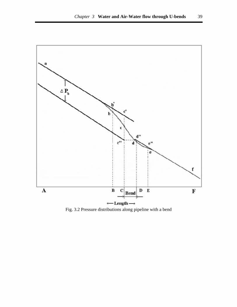
Chapter 3 Water and Air-Water flow through U-bends 39
Fig. 3.2 Pressure distributions along pipeline with a bend

Chapter 3 Water and Air-Water flow through U-bends 40
-350 -300 -250 -200 -150 -100 -50 0 50 100 150 200 2500
5
10
15
20
25
30
Radius of curvature : 0.11 m
Water flow rate : 5.42X10⁻⁴
m3/s
Symbol Air flow rate
(X104), m
3/s
0.901.271.702.613.083.433.774.264.524.93
Sta
tic P
ress
ure,
kP
a
Distance, cm Bend DownstreamUpstream
Fig. 3.3 Typical static pressure distribution curve

Chapter 3 Water and Air-Water flow through U-bends 41
Grid Size: Level: 0; Cells: 21344; Grid Size: Level: 0; Cells: 5076;
Faces: 65930; Nodes: 23616 Faces: 16656; Nodes: 6792;
Partitions: 1; 1 cell zone, Partitions: 1; 1 cell zone,
4 face zones 4 face zones
(a) Radius of curvature 0.06 m (b) Radius of curvature 0.11 m
Grid Size: Level: 0; Cells: 5076; Grid Size: Level: 0; Cells: 20240;
Faces: 16656; Nodes: 6792; Faces: 65364; Nodes: 25355;
Partitions: 1; 1 cell zone, 4 face zones Partitions: 1; 1 cell zone,
4 face zones
(c) Radius of curvature 0.15 m (d) Radius of curvature 0.20 m
Fig. 3.4 Grid for U-bends

Chapter 3 Water and Air-Water flow through U-bends 42
(a) Radius of curvature 0.06 m (b) Radius of curvatures 0.1 m
(c) Radius of curvature 0.15 m (d) Radius of curvatures 0.2 m
Fig. 3.5 Plot of velocity vector for U–bend for water velocity (m/s): 0.933

Chapter 3 Water and Air-Water flow through U-bends 43
(a) Radius of curvatures 0.06 m (b) Radius of curvatures 0.11 m
(c) Radius of curvatures 0.15 m (d) Radius of curvatures 0.2 m
Fig. 3.6 Plot of velocity vector in the bend portion, i.e., helicity for U–bends for watervelocity (m/s): 0.933

Chapter 3 Water and Air-Water flow through U-bends 44
Fig. 3.7 Contour plot of velocity vector at different points in the bend at water velocity(m/s): 0.933 and radius of curvature (m): 0.06

Chapter 3 Water and Air-Water flow through U-bends 45
Fig. 3.8 Contour plot of velocity vector at angular coordinates in the bend for watervelocity (m/s): 0.933 and radius of curvature (m): 0.06

Chapter 3 Water and Air-Water flow through U-bends 46
Fig. 3.9 Contour plot of velocity at different points in the bend for water velocity (m/s):0.933 and radius of curvature (m): 0.06
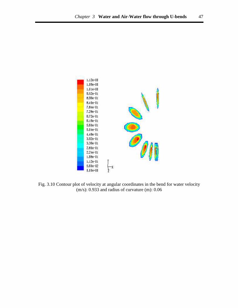
Chapter 3 Water and Air-Water flow through U-bends 47
Fig. 3.10 Contour plot of velocity at angular coordinates in the bend for water velocity(m/s): 0.933 and radius of curvature (m): 0.06

Chapter 3 Water and Air-Water flow through U-bends 48
Fig. 3.11 Contour plot of velocity at radial coordinates in the bend for water velocity(m/s): 0.933 and radius of curvature (m): 0.06
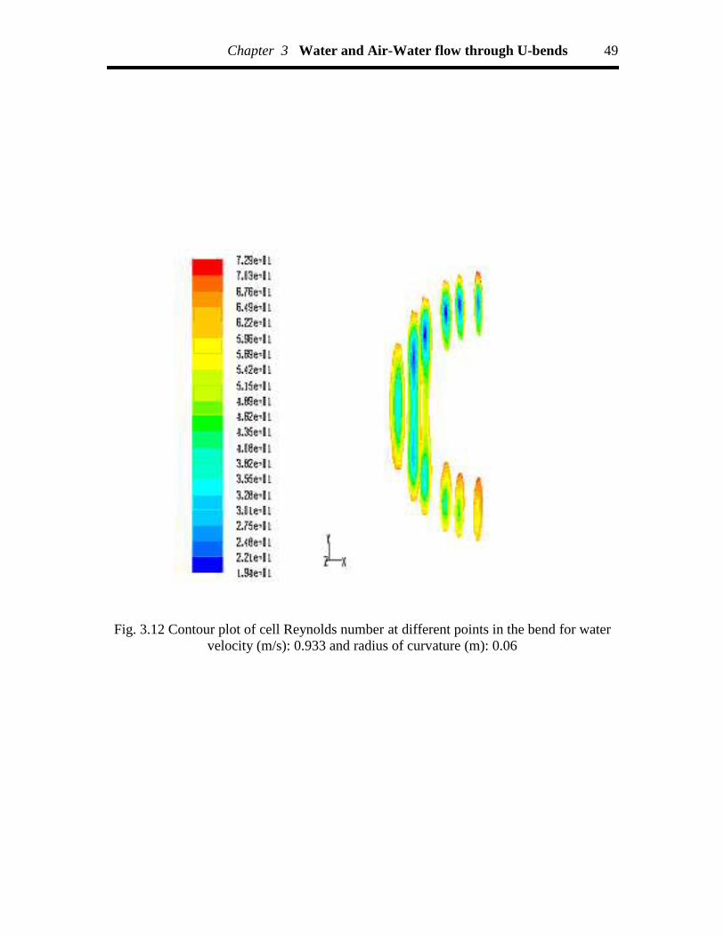
Chapter 3 Water and Air-Water flow through U-bends 49
Fig. 3.12 Contour plot of cell Reynolds number at different points in the bend for watervelocity (m/s): 0.933 and radius of curvature (m): 0.06

Chapter 3 Water and Air-Water flow through U-bends 50
Fig. 3.13 Contour plot of cell Reynolds number at angular coordinates in the bend forwater velocity (m/s): 0.933 and radius of curvature (m): 0.06

Chapter 3 Water and Air-Water flow through U-bends 51
Fig. 3.14 Contour plot of cell Reynolds number at radial coordinates in the bend for watervelocity (m/s): 0.933 and radius of curvature (m): 0.06
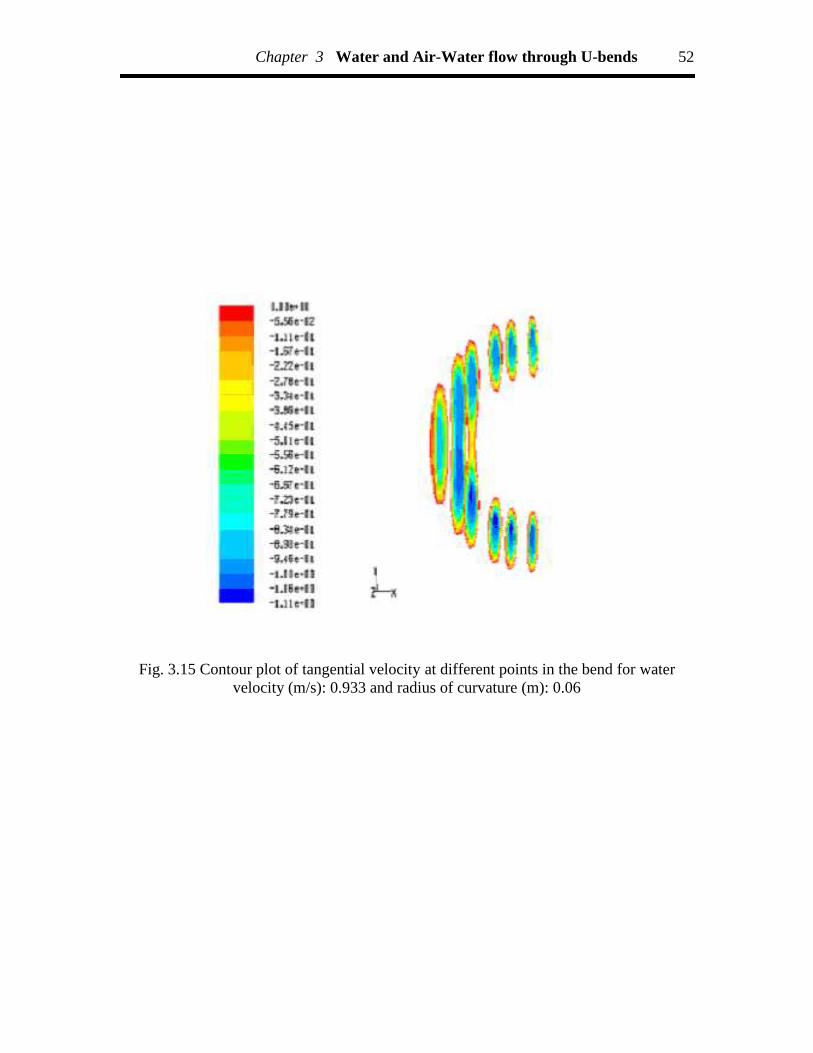
Chapter 3 Water and Air-Water flow through U-bends 52
Fig. 3.15 Contour plot of tangential velocity at different points in the bend for watervelocity (m/s): 0.933 and radius of curvature (m): 0.06

Chapter 3 Water and Air-Water flow through U-bends 53
Fig. 3.16 Contour plot of tangential velocity at angular coordinates in the bend for watervelocity (m/s): 0.933 and radius of curvature (m): 0.06
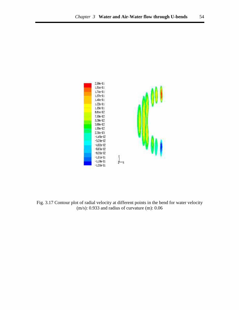
Chapter 3 Water and Air-Water flow through U-bends 54
Fig. 3.17 Contour plot of radial velocity at different points in the bend for water velocity(m/s): 0.933 and radius of curvature (m): 0.06

Chapter 3 Water and Air-Water flow through U-bends 55
Fig. 3.18 Contour plot of radial velocity at angular coordinates in the bend for watervelocity (m/s): 0.933 and radius of curvature (m): 0.06

Chapter 3 Water and Air-Water flow through U-bends 56
(a) Radius of curvatures 0.06 m (b) Radius of curvatures 0.11 m
(c) Radius of curvatures 0.15 m (d) Radius of curvatures 0.2 m
Fig. 3.19 Contours plot of static pressure for U–bend for water velocity (m/s): 0.933

Chapter 3 Water and Air-Water flow through U-bends 57
Fig. 3.20 Contour plot of static pressure at different points in the bend for water velocity(m/s): 0.933 and radius of curvature (m): 0.06

Chapter 3 Water and Air-Water flow through U-bends 58
Fig. 3.21 Contour plot of static pressure at angular coordinates in the bend for watervelocity (m/s): 0.933 and radius of curvature (m): 0.06

Chapter 3 Water and Air-Water flow through U-bends 59
Fig. 3.22 Contour plot of static pressure at radial coordinates in the bend for watervelocity (m/s): 0.933 and radius of curvature (m): 0.06

Chapter 3 Water and Air-Water flow through U-bends 60
Fig. 3.23 Contour velocity plot inside the different points of U-bend forwater velocity: 0.933 m/s, radius of curvature: 0.06 m
Fig. 3.24 Contour velocity plot inside the different angular points of U-bend forwater velocity: 0.933 m/s, radius of curvature: 0.06 m
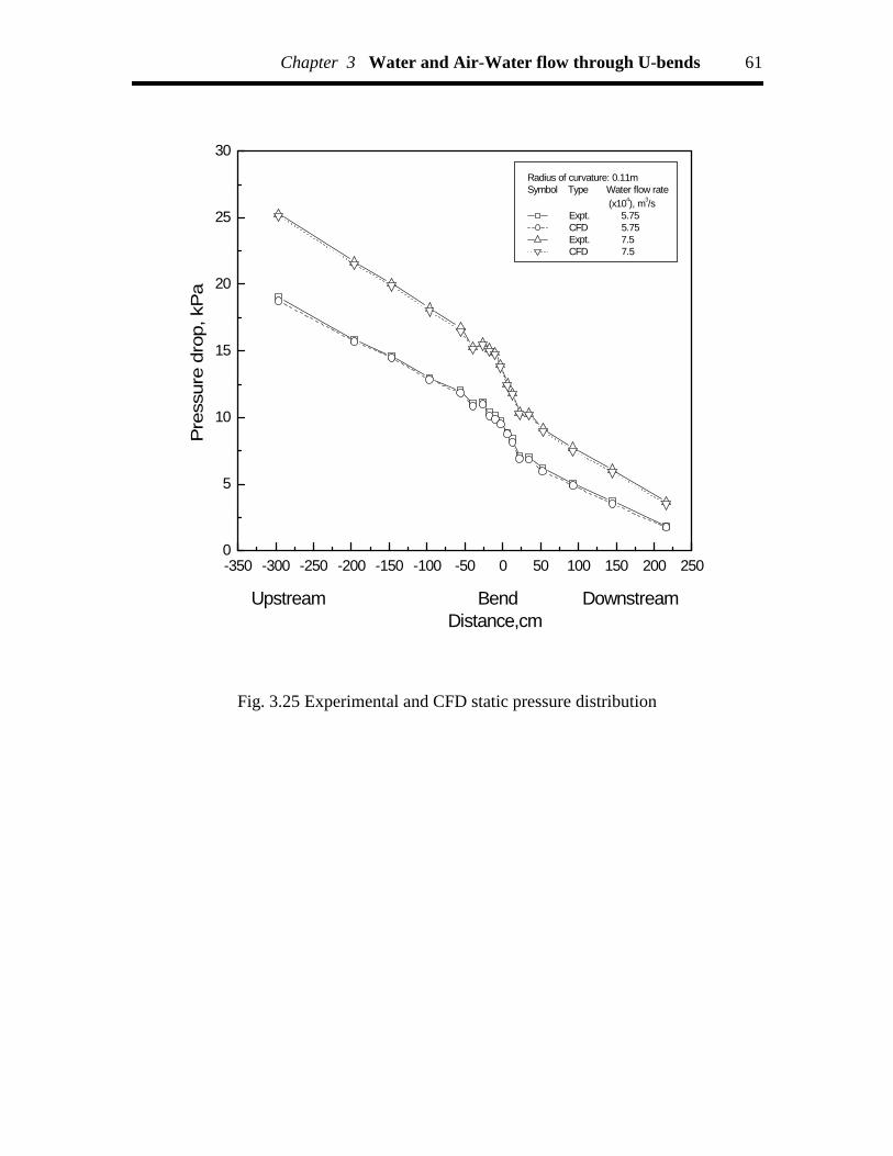
Chapter 3 Water and Air-Water flow through U-bends 61
-350 -300 -250 -200 -150 -100 -50 0 50 100 150 200 2500
5
10
15
20
25
30
Pre
ssur
e dr
op, k
Pa
Upstream Bend Downstream Distance,cm
Radius of curvature: 0.11mSymbol Type Water flow rate (x104), m3/s
Expt. 5.75 CFD 5.75 Expt. 7.5 CFD 7.5
Fig. 3.25 Experimental and CFD static pressure distribution

Chapter 3 Water and Air-Water flow through U-bends 62
(a) Radius of curvatures 0.06 m (b) Radius of curvatures 0.11 m
(c) Radius of curvatures 0.15 m (d) Radius of curvatures 0.2 m
Fig. 3.26 Contours plot of wall shear stress for U–bend for water velocity (m/s): 0.933

Chapter 3 Water and Air-Water flow through U-bends 63
Fig. 3.27 Contour plot of wall shear stress at different points in the bend forwater velocity: 0.933 m/s, radius of curvature: 0.06 m

Chapter 3 Water and Air-Water flow through U-bends 64
Fig. 3.28 Contour plot of wall shear stress at angular coordinates in the bend for watervelocity (m/s): 0.933, radius of curvature (m): 0.06

Chapter 3 Water and Air-Water flow through U-bends 65
Fig. 3.29 Contour plot of wall shear stress at radial coordinates in the bend for watervelocity (m/s): 0.933, radius of curvature (m): 0.06

Chapter 3 Water and Air-Water flow through U-bends 66
(a) Radius of curvatures 0.06 m (b) Radius of curvatures 0.11 m
(c) Radius of curvatures 0.15 m (d) Radius of curvatures 0.20 m

Chapter 3 Water and Air-Water flow through U-bends 67
Fig. 3.30 Contours plot of strain rate for U–bend for water velocity (m/s): 0.933
Fig. 3.31 Contour plot of wall strain rate at different points in the bendfor water velocity (m/s): 0.933, radius of curvature (m): 0.06
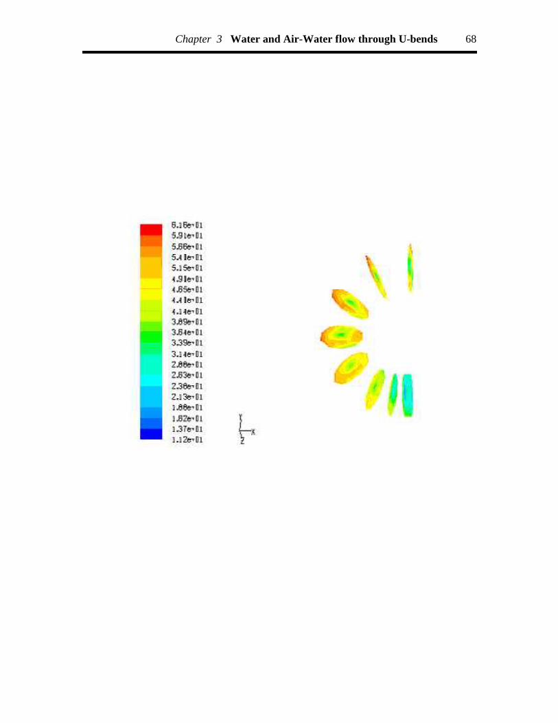
Chapter 3 Water and Air-Water flow through U-bends 68
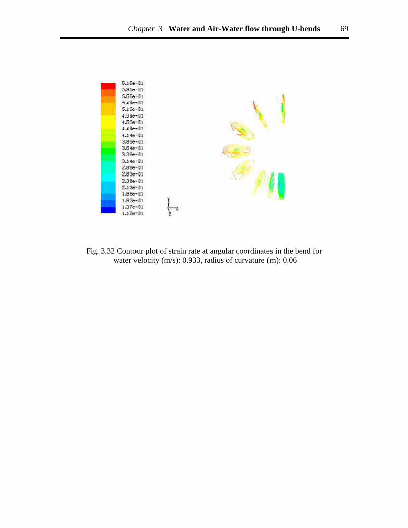
Chapter 3 Water and Air-Water flow through U-bends 69
Fig. 3.32 Contour plot of strain rate at angular coordinates in the bend forwater velocity (m/s): 0.933, radius of curvature (m): 0.06

Chapter 3 Water and Air-Water flow through U-bends 70
Fig.3.33 Contour plot of strain rate at radial coordinates in the bend forwater velocity (m/s): 0.933, radius of curvature (m): 0.06

Chapter 3 Water and Air-Water flow through U-bends 71
Fig. 3.34 Contour plot of helicity at different points in the bend forwater velocity (m/s): 0.933, radius of curvature (m): 0.06
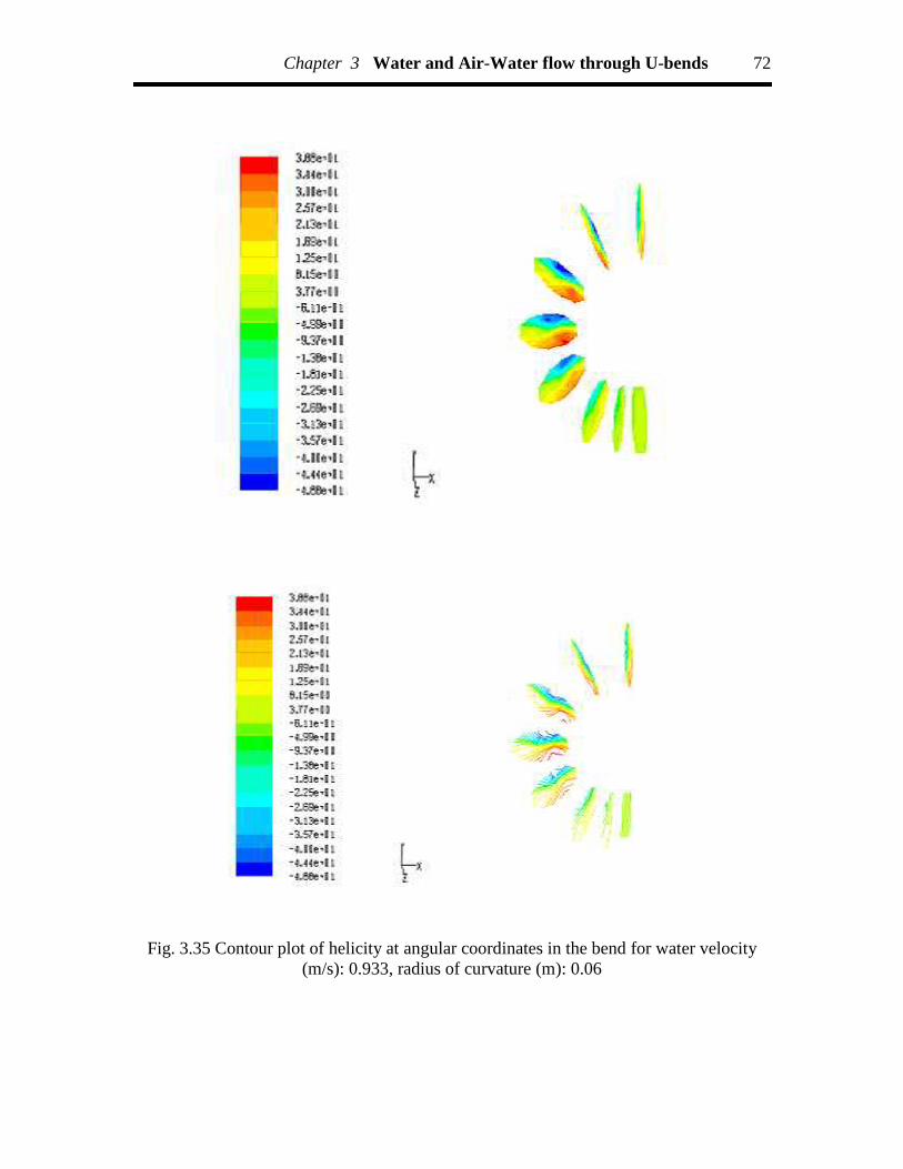
Chapter 3 Water and Air-Water flow through U-bends 72
Fig. 3.35 Contour plot of helicity at angular coordinates in the bend for water velocity(m/s): 0.933, radius of curvature (m): 0.06
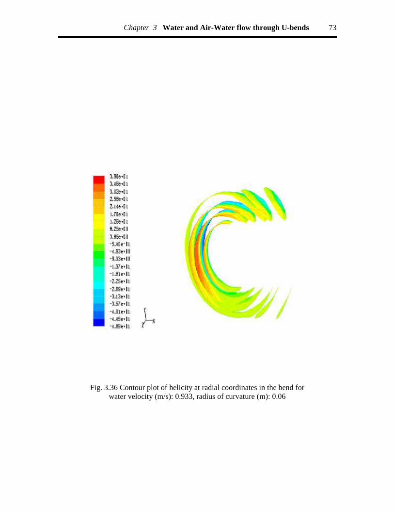
Chapter 3 Water and Air-Water flow through U-bends 73
Fig. 3.36 Contour plot of helicity at radial coordinates in the bend forwater velocity (m/s): 0.933, radius of curvature (m): 0.06

Chapter 3 Water and Air-Water flow through U-bends 74
Fig. 3.37 Contour plot of vorticity at different points in the bend forwater velocity (m/s): 0.933, radius of curvature (m): 0.06
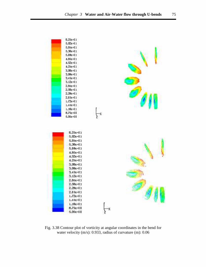
Chapter 3 Water and Air-Water flow through U-bends 75
Fig. 3.38 Contour plot of vorticity at angular coordinates in the bend forwater velocity (m/s): 0.933, radius of curvature (m): 0.06

Chapter 3 Water and Air-Water flow through U-bends 76
Fig. 3.39 Contour plot of vorticity at radial coordinates in the bend forwater velocity (m/s): 0.933, radius of curvature (m): 0.06

Chapter 3 Water and Air-Water flow through U-bends 77
Fig. 3.40 Contour plot of turbulent kinetic energy at different points in the bend forwater velocity (m/s): 0.933, radius of curvature (m): 0.06
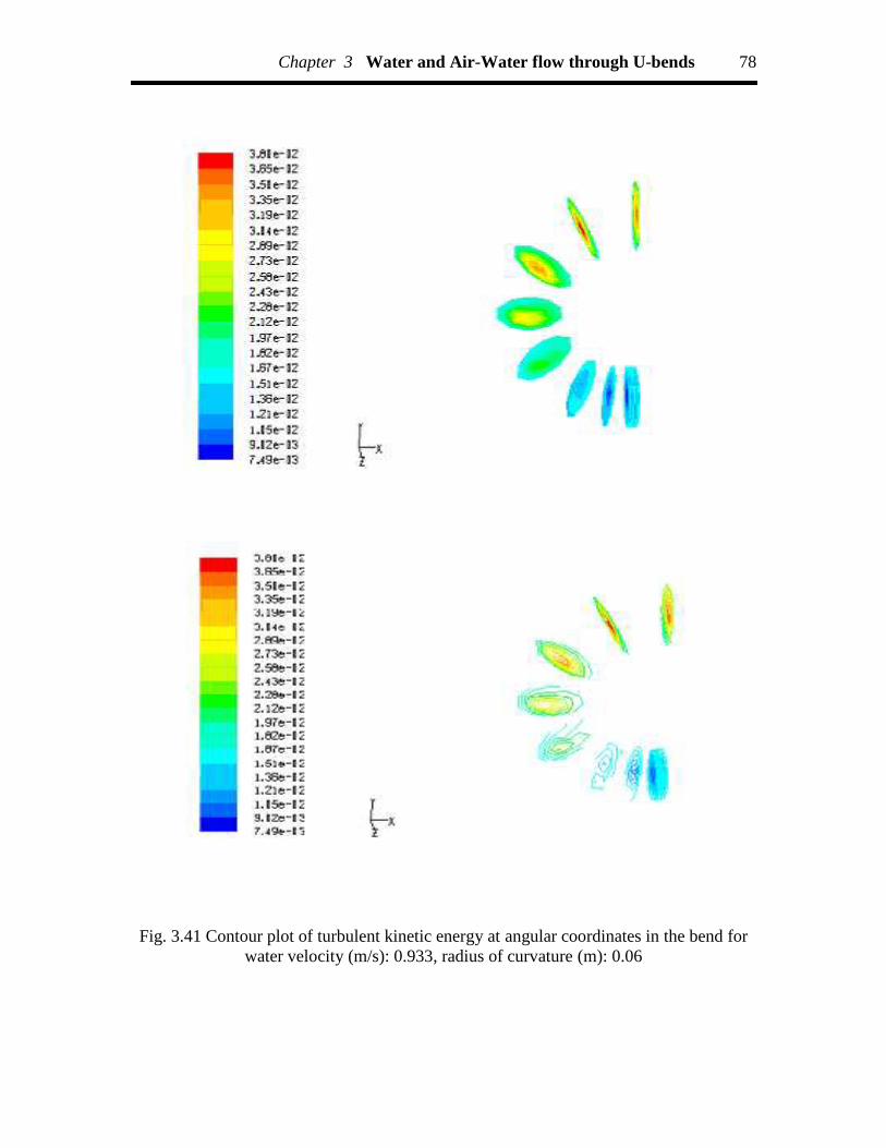
Chapter 3 Water and Air-Water flow through U-bends 78
Fig. 3.41 Contour plot of turbulent kinetic energy at angular coordinates in the bend forwater velocity (m/s): 0.933, radius of curvature (m): 0.06

Chapter 3 Water and Air-Water flow through U-bends 79
Fig. 3.42 Contour plot of turbulent kinetic energy at radial coordinates in the bend forwater velocity (m/s): 0.933, radius of curvature (m): 0.06
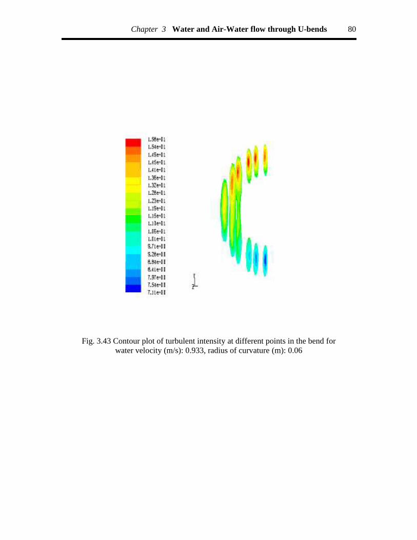
Chapter 3 Water and Air-Water flow through U-bends 80
Fig. 3.43 Contour plot of turbulent intensity at different points in the bend forwater velocity (m/s): 0.933, radius of curvature (m): 0.06

Chapter 3 Water and Air-Water flow through U-bends 81
Fig. 3.44 Contour plot of turbulent intensity at angular coordinates in the bend forwater velocity (m/s): 0.933, radius of curvature (m): 0.06
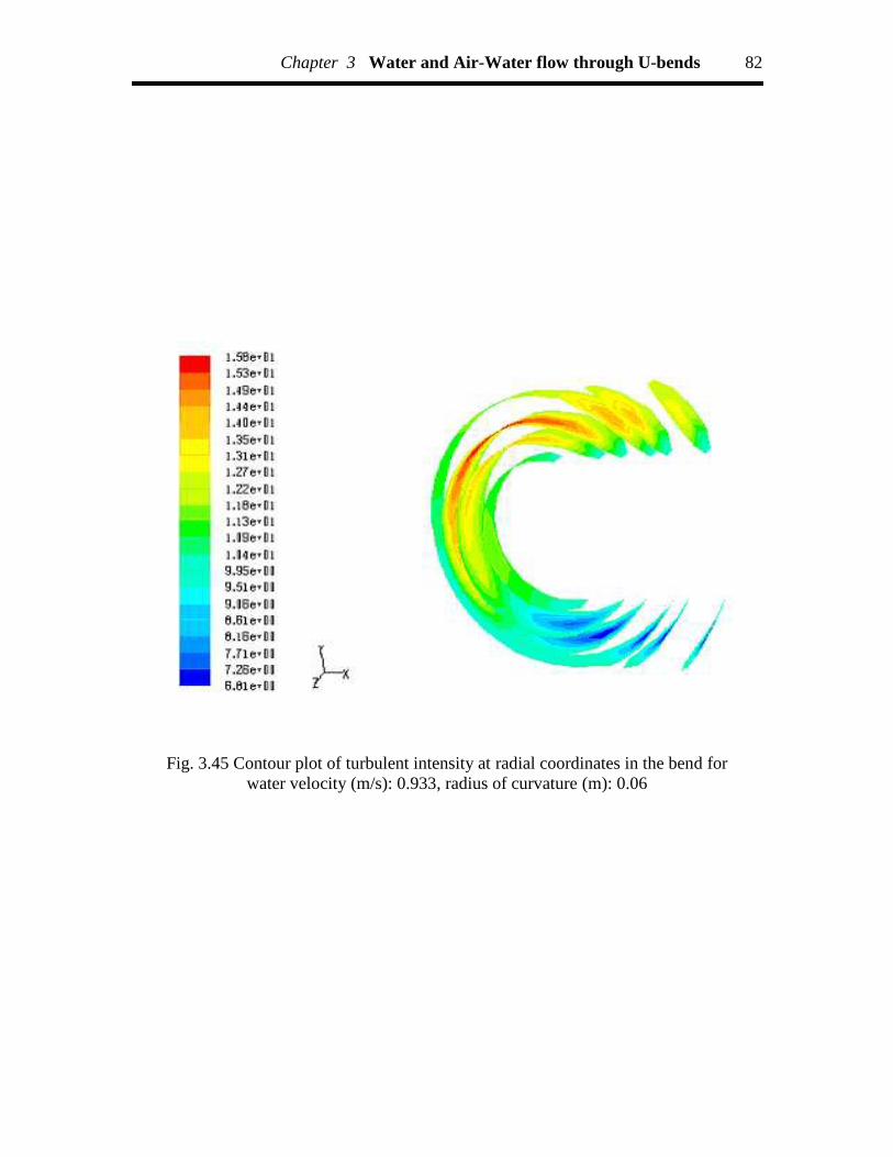
Chapter 3 Water and Air-Water flow through U-bends 82
Fig. 3.45 Contour plot of turbulent intensity at radial coordinates in the bend forwater velocity (m/s): 0.933, radius of curvature (m): 0.06

Chapter 3 Water and Air-Water flow through U-bends 83
Fig. 3.46 Contour plot of turbulent dissipation rate at different points in the bend forwater velocity (m/s): 0.933, radius of curvature (m): 0.06
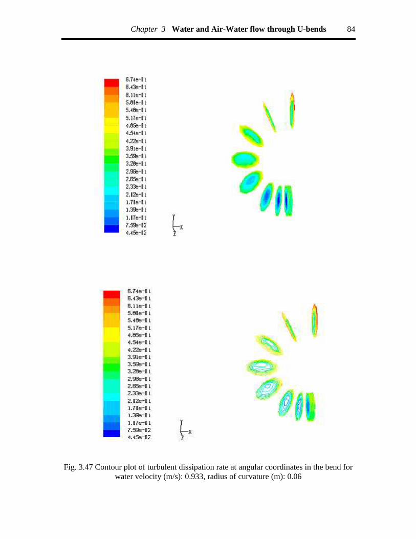
Chapter 3 Water and Air-Water flow through U-bends 84
Fig. 3.47 Contour plot of turbulent dissipation rate at angular coordinates in the bend forwater velocity (m/s): 0.933, radius of curvature (m): 0.06
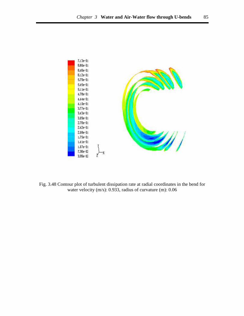
Chapter 3 Water and Air-Water flow through U-bends 85
Fig. 3.48 Contour plot of turbulent dissipation rate at radial coordinates in the bend forwater velocity (m/s): 0.933, radius of curvature (m): 0.06

Chapter 3 Water and Air-Water flow through U-bends 86
Fig. 3.49 Contour plot of production of k at different points in the bend forwater velocity (m/s): 0.933, radius of curvature (m): 0.06

Chapter 3 Water and Air-Water flow through U-bends 87
Fig. 3.50 Contour plot of production of k at angular coordinates in the bend forwater velocity (m/s): 0.933, radius of curvature (m): 0.06

Chapter 3 Water and Air-Water flow through U-bends 88
Fig. 3.51 Contour plot of turbulent viscosity at different points in the bend forwater velocity (m/s): 0.933, radius of curvature (m): 0.06
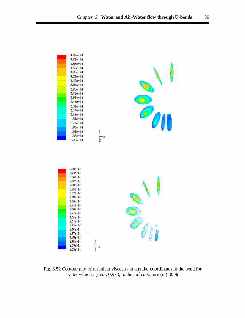
Chapter 3 Water and Air-Water flow through U-bends 89
Fig. 3.52 Contour plot of turbulent viscosity at angular coordinates in the bend forwater velocity (m/s): 0.933, radius of curvature (m): 0.06

Chapter 3 Water and Air-Water flow through U-bends 90
Fig. 3.53 Contour plot of turbulent viscosity at radial coordinates in the bend forwater velocity (m/s): 0.933, radius of curvature (m): 0.06

Chapter 3 Water and Air-Water flow through U-bends 91
Fig. 3.54 Contour plot of mass imbalance at radial coordinates in the bend for watervelocity (m/s): 0.933, radius of curvature (m): 0.06
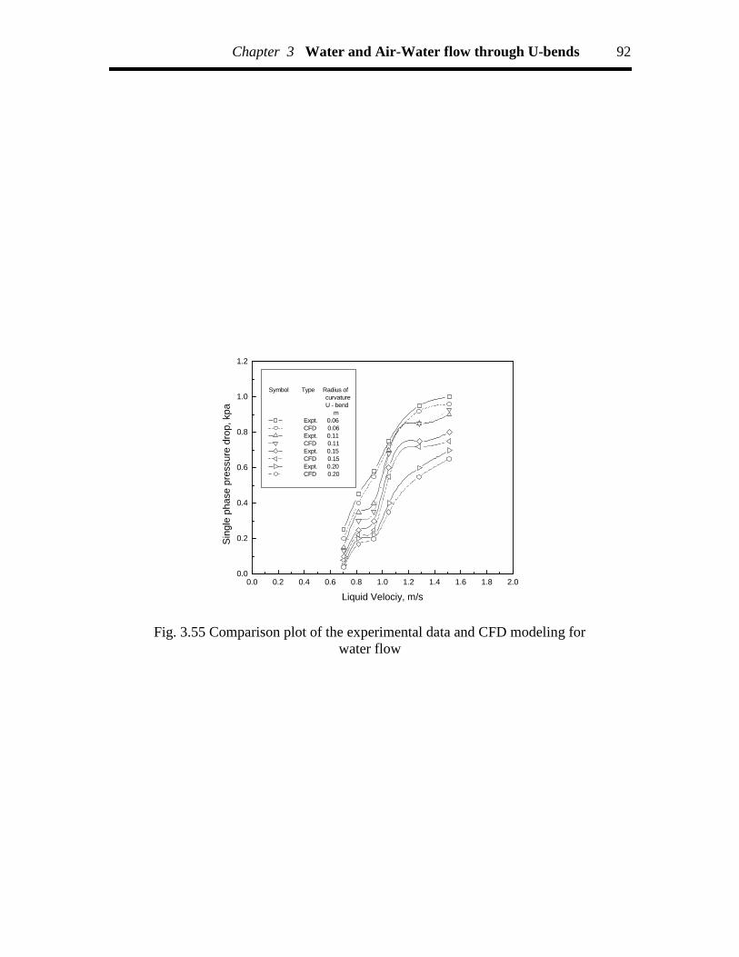
Chapter 3 Water and Air-Water flow through U-bends 92
0.0 0.2 0.4 0.6 0.8 1.0 1.2 1.4 1.6 1.8 2.00.0
0.2
0.4
0.6
0.8
1.0
1.2
Sing
le p
hase
pre
ssur
e dr
op, k
pa
Liquid Velociy, m/s
Symbol Type Radius of curvature U - bend m
Expt. 0.06 CFD 0.06 Expt. 0.11 CFD 0.11 Expt. 0.15 CFD 0.15 Expt. 0.20 CFD 0.20
Fig. 3.55 Comparison plot of the experimental data and CFD modeling forwater flow

Chapter 3 Water and Air-Water flow through U-bends 93
(a) Radius of curvature 0.06 m (b) Radius of curvatures 0.11 m

Chapter 3 Water and Air-Water flow through U-bends 94
(c) Radius of curvature 0.15 m (d) Radius of curvatures 0.2 m
Fig. 3.56 Contour plot of velocity vector for U–bend, water velocity (m/s): 0.933, gasvelocity (m/s): 1.365, gas fraction, g : 0.59
Fig. 3.57a Contour plot of velocity vector for air-water mixture at differentpoints in the bend,

Chapter 3 Water and Air-Water flow through U-bends 95
radius of curvature 0.06 m, water velocity (m/s): 0.933,gas velocity (m/s): 1.365, gas fraction, g : 0.5

Chapter 3 Water and Air-Water flow through U-bends 96
Fig. 3.57b Contour plot of velocity vector for water in the mixture at differentpoints in the bend,
radius of curvature 0.06 m, water velocity (m/s): 0.933,gas velocity (m/s): 1.365, gas fraction, g : 0.59
Fig. 3.57c Contour plot of velocity vector for air in the mixture at differentpoints in the bend,
radius of curvature 0.06 m, water velocity (m/s): 0.933,
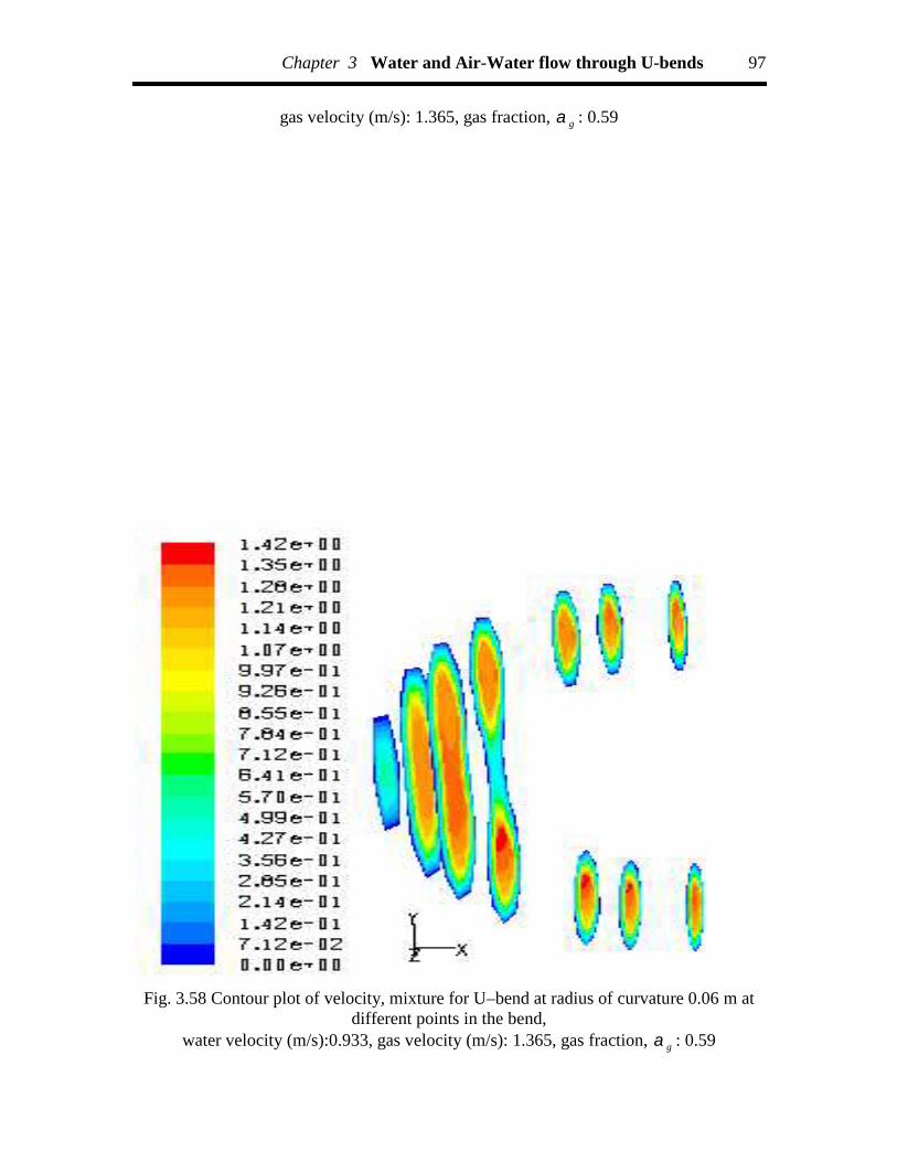
Chapter 3 Water and Air-Water flow through U-bends 97
gas velocity (m/s): 1.365, gas fraction, g : 0.59
Fig. 3.58 Contour plot of velocity, mixture for U–bend at radius of curvature 0.06 m atdifferent points in the bend,
water velocity (m/s):0.933, gas velocity (m/s): 1.365, gas fraction, g : 0.59

Chapter 3 Water and Air-Water flow through U-bends 98

Chapter 3 Water and Air-Water flow through U-bends 99
Fig. 3.59 Contour plot of velocity, mixture for U–bend at radius of curvature 0.06 m atdifferent angular points in the bend,
water velocity (m/s): 0.933, gas velocity(m/s): 1.365, gas fraction, g : 0.59
a) Radius of curvature 0.06 m (b) Radius of curvatures 0.11 m
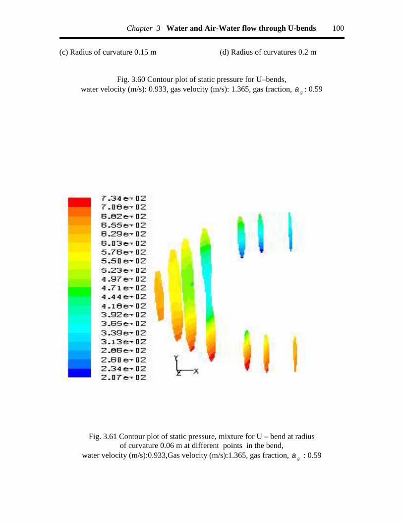
Chapter 3 Water and Air-Water flow through U-bends 100
(c) Radius of curvature 0.15 m (d) Radius of curvatures 0.2 m
Fig. 3.60 Contour plot of static pressure for U–bends,water velocity (m/s): 0.933, gas velocity (m/s): 1.365, gas fraction, g : 0.59
Fig. 3.61 Contour plot of static pressure, mixture for U – bend at radiusof curvature 0.06 m at different points in the bend,
water velocity (m/s):0.933,Gas velocity (m/s):1.365, gas fraction, g : 0.59
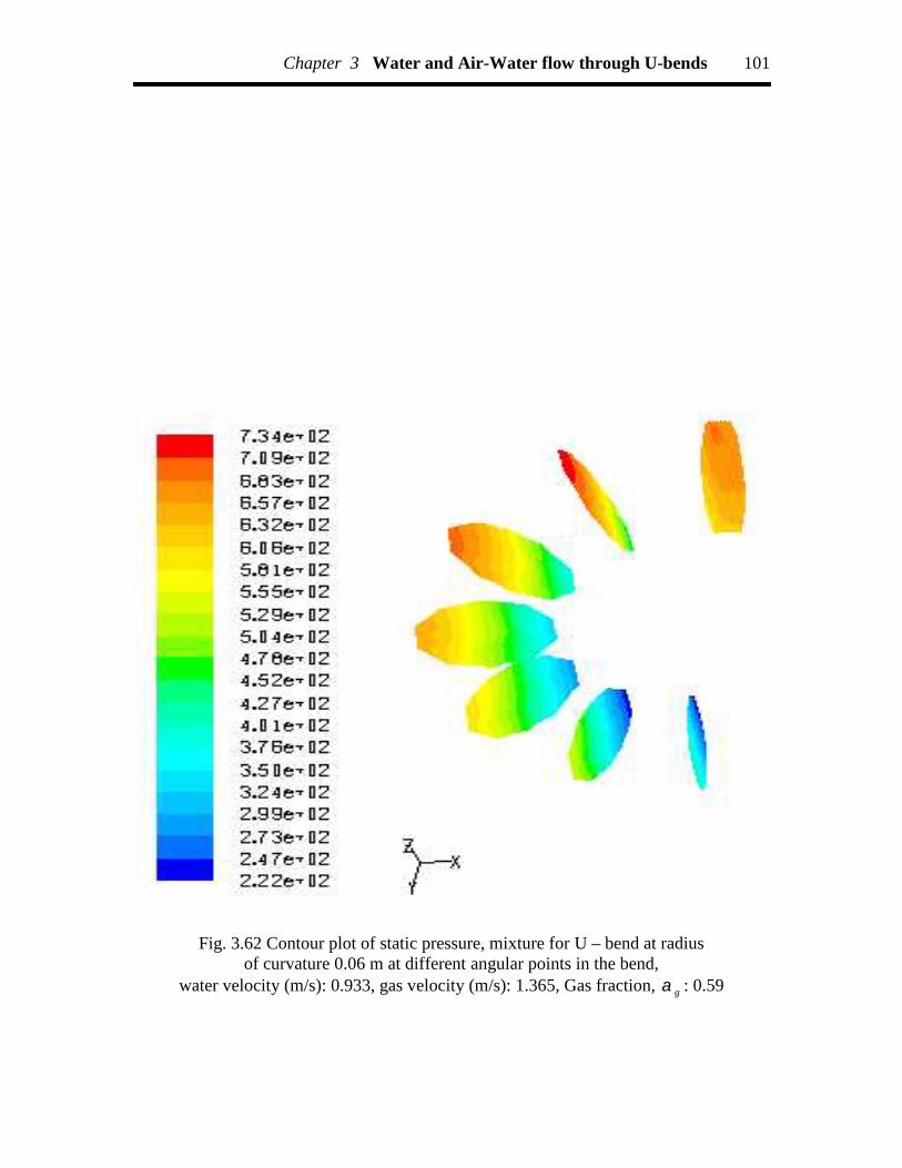
Chapter 3 Water and Air-Water flow through U-bends 101
Fig. 3.62 Contour plot of static pressure, mixture for U – bend at radiusof curvature 0.06 m at different angular points in the bend,
water velocity (m/s): 0.933, gas velocity (m/s): 1.365, Gas fraction, g : 0.59
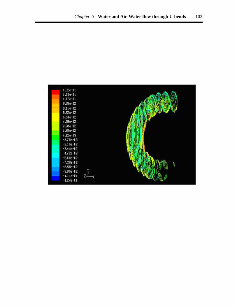
Chapter 3 Water and Air-Water flow through U-bends 102

Chapter 3 Water and Air-Water flow through U-bends 103
Fig. 3.63 Contour velocity plot inside the different points of U-bend,water velocity: 0.933 m/s, gas velocity (m/s): 1.365, Gas fraction, g : 0.59, radius of
curvature: 0.06 m

Chapter 3 Water and Air-Water flow through U-bends 104
Fig. 3.64 Contour velocity plot inside the different angular points of U-bendwater velocity: 0.933 m/s, gas velocity (m/s): 1.365, Gas fraction, g : 0.59, radius of
curvature: 0.06 m

Chapter 3 Water and Air-Water flow through U-bends 105
-350 -300 -250 -200 -150 -100 -50 0 50 100 150 200 2500
5
10
15
20
25
30
Sta
tic P
ress
ure,
kP
a
Upstream Bend Downstream Distance, cm
Radius of curvature: 0.11mWater flow rate: 5.42x10⁻⁴ m3/sSymbol Type Air flow rate (x104 ), m3/s
Expt. 0.90 CFD 0.90 Expt. 1.29 CFD 1.29 Expt. 1.70 CFD 1.70
Fig. 3.65 Experimental and CFD static pressure distribution

Chapter 3 Water and Air-Water flow through U-bends 106
Fig. 3.66a Contour plot of volume fraction for water at different points in the bend,radius of curvature 0.06 m, water velocity (m/s): 0.933,
gas velocity (m/s): 1.365, gas fraction, g : 0.59
(b) air
Fig. 3.66b Contour plot of volume fraction for air at different points in the bend,radius of curvature 0.06 m, water velocity (m/s): 0.933,
gas velocity (m/s): 1.365, gas fraction, g : 0.59

Chapter 3 Water and Air-Water flow through U-bends 107
Fig. 3.67a Contour plot of volume fraction for water at differentangular points in the bend,
radius of curvature 0.06 m, water velocity (m/s): 0.933,gas velocity (m/s): 1.365, gas fraction, g : 0.59
Fig. 3.67b Contour plot of volume fraction for air at angular coordinates in the bend,radius of curvature 0.06 m, water velocity (m/s): 0.933,
gas velocity (m/s): 1.365, gas fraction, g : 0.59
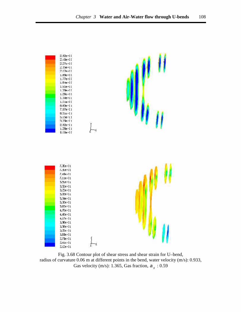
Chapter 3 Water and Air-Water flow through U-bends 108
Fig. 3.68 Contour plot of shear stress and shear strain for U–bend,radius of curvature 0.06 m at different points in the bend, water velocity (m/s): 0.933,
Gas velocity (m/s): 1.365, Gas fraction, g : 0.59

Chapter 3 Water and Air-Water flow through U-bends 109
0.0 0.3 0.6 0.9 1.2 1.50
2
4
6
8
Two-
phas
e Pr
essu
re D
rop,
Kpa
Velocity of Air(m /s)
Radius of Curvature ofU - bend: 0.11mSymbol Type Velocity of water (m/s)
Expt. 0.702 CFD 0.702 Expt. 0.816 CFD 0.816 Expt. 0.933 CFD 0.933
Fig. 3.69 Comparison plot of the experimental data and CFD modeling for two–phaseair–water flow

Chapter 3 Water and Air-Water flow through U-bends 110
0.2 0.4 0.6 0.8 1.0 1.2 1.41.0
1.5
2.0
2.5
3.0
3.5
4.0
4.5
5.0
Tw
o - ph
ase
pres
sure
dro
p, K
pa
Gas Velocity, m/s
Liquid Velocity of U - bend: 0.702 m/sSymbol Type Radius of Curvature,m
Expt. 0.06 CFD 0.06 Expt. 0.11 CFD 0.11 Expt. 0.15 CFD 0.15 Expt. 0.20 CFD 0.20
Fig. 3.70 Comparison plot of the experimental data and CFD modeling of two–phaseair–water flow

Chapter 3 Water and Air-Water flow through U-bends 111
Table 3.1 Dimensions of the U-bends used in the experiments
Sl. No. Radius of curvature, m Length of the bend, m
1. 0.06 0.1885
2. 0.11 0.3456
3. 0.15 0.4712
4. 0.20 0.6283
Table 3.2 Range of variables used in the experiments
U-bendsMeasurement Type Range
Diameter (m) 0.01905Radius of curvature (m) 0.06 ≤ Rb ≤ 0.20
Liquid and Flow properties
Water Flow Rate Ql×10-4(m3/s) 2.000 to 4.65
Air Flow Rate Qg×10-5(m3/s) 5.936 to 56.1189

Chapter 3 Water and Air-Water flow through U-bends 112
Table 3.3 Comparison of the pressure drop across the U-bends,Experimental and CFD analysis data
Sl.No.
Watervelocity
Vl
m/s
Pressuredrop,
experimental
.,ExptbPkPa
Pressuredrop,CFD
,b CFDPkPa
Radius of curvature of U-bend: 0.06m1 0.702 0.25 0.22 0.816 0.45 0.43 0.933 0.58 0.54 1.049 0.75 0.725 1.281 0.95 0.96 1.512 1.00 0.96
Radius of curvature of U-bend: 0.11m
7 0.702 0.15 0.138 0.816 0.35 0.309 0.933 0.40 0.35
10 1.049 0.70 0.6811 1.281 0.85 0.8012 1.512 0.90 0.88
Radius of curvature of U-bend: 0.15m13 0.702 0.10 0.0814 0.816 0.25 0.2215 0.933 0.30 0.2516 1.049 0.60 0.5017 1.281 0.75 0.7018 1.512 0.80 0.75
Radius of curvature of U-bend: 0.2m19 0.702 0.05 0.0420 0.816 0.20 0.1721 0.933 0.22 0.2022 1.049 0.40 0.3523 1.281 0.60 0.5524 1.512 0.70 0.65

Chapter 3 Water and Air-Water flow through U-bends 113
Table 3.4 Comparison of the two-phase pressure drop across the U-bends,Experimental and CFD analysis
Sl.No.
Air velocity
Vg
m/s
Two-phasepressure
dropP tplb, Expt.
kPa
Two-phasepressure
drop
CFDtplbP ,kPa
Water velocity, Vl : 0.702 m/sRadius of crvature: 0.06m
1 0.273 2.651 2.552 0.612 3.535 3.53 0.831 3.777 3.774 1.119 3.882 3.9
Water velocity, Vl : 0.702 m/sRadius of curvature: 0.11m
5 0.276 1.427 1.46 0.611 1.735 1.77 0.786 1.967 1.98 1.081 2.577 2.65
Water velocity, Vl : 0.702 m/sRadius of curvature: 0.15m
9 0.248 0.99 0.9510 0.639 0.131 1.1211 0.829 1.555 1.512 1.015 1.555 1.52
Water velocity, Vl : 0.702 m/sRadius of curvature: 0.2m
13 0.303 1.166 1.1414 0.65 1.379 1.3515 1.111 2.174 2.1516 1.285 2.374 2.36

Chapter 4
Non-Newtonian fluid flow through piping components –experimental investigation

Chapter 4 Non-Newtonian fluid flow through piping components 113
Experimental investigation have been carried out to evaluate the frictional
pressure drop across different piping components such as orifices, gate and globe valves,
elbows and bends in 0.0127 m piping components for non-Newtonian liquid flow.
Empirical correlations have been developed for the prediction of the frictional pressure
drop in terms of the various physical and dynamic variables of the system.
4.1 Introduction
Pipe fittings like valves, bends, elbows, tees, reducers, expander etc. are the
integral part of any piping system. Flow through piping components is more complex
than the straight pipes. The problem of determining the pressure losses in pipe fittings is
important in design and analysis of the fluid machinery. Forcing a fluid through pipe
fittings consumes energy detected by the drop in pressure across the fittings. The friction
between the fluid and the fitting wall causes this pressure drop. The problem of
predicting pressure losses in pipe fittings is much more uncertain than for the pipe
because,
1. The mechanism of flow is not clearly defined. At least two types of losses
are superposed – skin friction and loss due to change in flow direction, and
2. There are very few experimental data available in the literature.
Edwards et al. (1985) studied the frictional head loss of different fittings like 90o
elbows, gate valves, square plug and circular plug globe valves, expansions and
contractions, orifice plates in 2.54 cm and 5 cm pipeline for the flow of non-Newtonian
liquids. They observed that the loss coefficient depends on the size of the pipe fittings.
Das et al. (1991b) reported the experimental investigation of the pressure loss across
different types of bends in the horizontal plane for non-Newtonian liquids. They
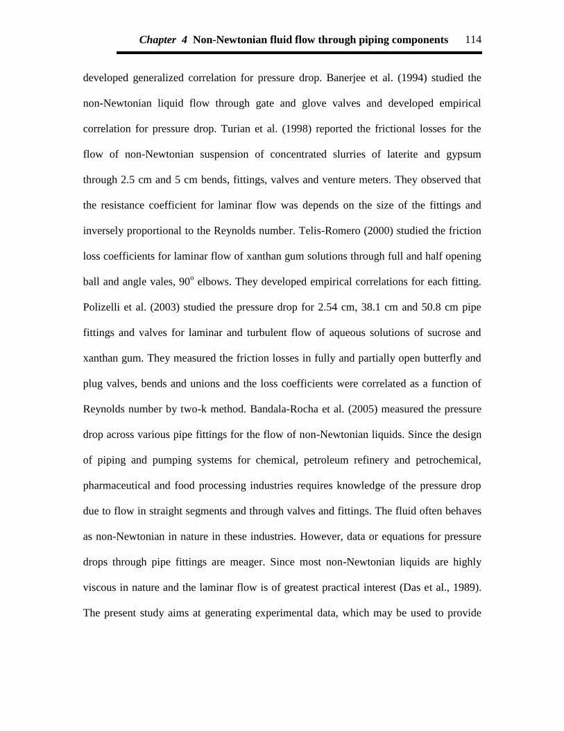
Chapter 4 Non-Newtonian fluid flow through piping components 114
developed generalized correlation for pressure drop. Banerjee et al. (1994) studied the
non-Newtonian liquid flow through gate and glove valves and developed empirical
correlation for pressure drop. Turian et al. (1998) reported the frictional losses for the
flow of non-Newtonian suspension of concentrated slurries of laterite and gypsum
through 2.5 cm and 5 cm bends, fittings, valves and venture meters. They observed that
the resistance coefficient for laminar flow was depends on the size of the fittings and
inversely proportional to the Reynolds number. Telis-Romero (2000) studied the friction
loss coefficients for laminar flow of xanthan gum solutions through full and half opening
ball and angle vales, 90o elbows. They developed empirical correlations for each fitting.
Polizelli et al. (2003) studied the pressure drop for 2.54 cm, 38.1 cm and 50.8 cm pipe
fittings and valves for laminar and turbulent flow of aqueous solutions of sucrose and
xanthan gum. They measured the friction losses in fully and partially open butterfly and
plug valves, bends and unions and the loss coefficients were correlated as a function of
Reynolds number by two-k method. Bandala-Rocha et al. (2005) measured the pressure
drop across various pipe fittings for the flow of non-Newtonian liquids. Since the design
of piping and pumping systems for chemical, petroleum refinery and petrochemical,
pharmaceutical and food processing industries requires knowledge of the pressure drop
due to flow in straight segments and through valves and fittings. The fluid often behaves
as non-Newtonian in nature in these industries. However, data or equations for pressure
drops through pipe fittings are meager. Since most non-Newtonian liquids are highly
viscous in nature and the laminar flow is of greatest practical interest (Das et al., 1989).
The present study aims at generating experimental data, which may be used to provide

Chapter 4 Non-Newtonian fluid flow through piping components 115
numerical correlations to predict pressure, drop through different pipe fittings for laminar
flow of non-Newtonian liquids.
4.2 The experimental setup
The schematic diagram of the experimental setup consists of elbow is shown in
Fig. 4.1. It consists of a liquid storage tank (0.45 m3), test section, control and measuring
systems for flow rates, pressure and other accessories. The test section consists of a
horizontal upstream straight tube of 4.5 m length, a test section and a horizontal
downstream straight tube of 3 m length. The reason for having long horizontal upstream
and downstream portions before and after the test section was to achieve fully developed
flow conditions to facilitate the measurement of pressure across the test section. The test
section was connected to the upstream and downstream portions with the help of flanges.
The entrance and exit lengths were 2.0 m and 1.4 m respectively, which were more than
50 pipe diameters to ensure fully developed flow. Before the test section, a 0.5 m length
Perspex tube of the same diameter was incorporated in the system for flow visualization.
The rest of the test section was fabricated from mild steel. The test section was fitted
horizontally with the help of a leveling gauge. It was provided with pressure taps
(piezometric ring) at different points in the upstream and downstream sections of the
pipe. Different types of pipe fittings have been used and their dimensions are given in
Table 4.1. The elbows and orifices used were specially manufactured in order to ensure
uniform internal diameter, constant curvature and roundness. The gate and globe valves
used in the experiments are made of steel used in petroleum, petrochemical and allied
industries and they satisfy the Indian standard IS: 10605-1983 and IS : 11335-1984
respectively.
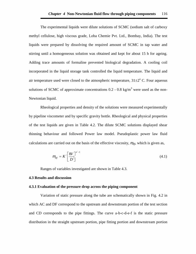
Chapter 4 Non-Newtonian fluid flow through piping components 116
The experimental liquids were dilute solutions of SCMC (sodium salt of carboxy
methyl cellulose, high viscous grade, Loba Chemie Pvt. Ltd., Bombay, India). The test
liquids were prepared by dissolving the required amount of SCMC in tap water and
stirring until a homogeneous solution was obtained and kept for about 15 h for ageing.
Adding trace amounts of formaline prevented biological degradation. A cooling coil
incorporated in the liquid storage tank controlled the liquid temperature. The liquid and
air temperature used were closed to the atmospheric temperature, 312o C. Four aqueous
solutions of SCMC of approximate concentrations 0.2 - 0.8 kg/m3 were used as the non-
Newtonian liquid.
Rheological properties and density of the solutions were measured experimentally
by pipeline viscometer and by specific gravity bottle. Rheological and physical properties
of the test liquids are given in Table 4.2. The dilute SCMC solutions displayed shear
thinning behaviour and followed Power law model. Pseudoplastic power law fluid
calculations are carried out on the basis of the effective viscosity, eff, which is given as,
1/
/
8
n
eff D
VK (4.1)
Ranges of variables investigated are shown in Table 4.3.
4.3 Results and discussion
4.3.1 Evaluation of the pressure drop across the piping component
Variation of static pressure along the tube are schematically shown in Fig. 4.2 in
which AC and DF correspond to the upstream and downstream portion of the test section
and CD corresponds to the pipe fittings. The curve a-b-c-d-e-f is the static pressure
distribution in the straight upstream portion, pipe fitting portion and downstream portion

Chapter 4 Non-Newtonian fluid flow through piping components 117
of the test section. Pressure drop across the pipefitting, Ppf, was obtained from the
difference between the static pressure of the upstream, and the static pressure of the
downstream. Thus, Ppf, the frictional pressure drop across the pipe fitting for the
flowing fluid through a passage of length equal to the axis of the pipe fitting and the
additional pressure loss due to irreversibility. The typical static pressure distribution
curves are shown in Figs. 4.3 - 4.6.
4.3.2 Effect of non-Newtonian characteristics on the pressure drop across the pipingcomponents
Figs. 4.7 - 4.10 show the pressure drop across the different pipe fittings as a
function of liquid flow rate. It is clear from the graphs that as n/ decreases the pressure
drop increases at constant liquid flow rate.
4.3.3 Problem analysis
For flow of non-Newtonian fluid through a straight pipe, the steady state Z-
component equation of motion in cylindrical coordinate system in a horizontal pipe may
be written as
Zrr
r
rZ
P
Z
VV
V
r
V
r
VV zzzrzz
zzz
r
11(4.2)
This equation is dimensionally homogeneous and is true for laminar flow only. The
dimensional equality (numerically not true) for the equation may be written as,
L
V
L
P
L
V
2
(4.3)

Chapter 4 Non-Newtonian fluid flow through piping components 118
this equation is made dimensionless by dividing by V2/L which suggests that the
functional relationship of P with other parameters is as follows :
DV
FV
P2
(4.4)
Equation (4) is only true for flow in a horizontal straight pipe.
4.3.3.1 Elbow
Fluid flowing through a straight pipe attains a characteristic velocity profile that is
independent of the distance along the pipe, i.e., the flow becomes fully developed. If the
flow direction is changed with a curved pipe, the flow structure of the fluid is completely
changed. The fluid is subjected to varying degrees of centrifugal forces from the
neighborhood of the curved wall to the center of the pipe. Due to the interaction primarily
between centrifugal and viscous forces in the curved portion of the flow, certain
characteristic motion, known as secondary flow, is generated which causes shifting of the
maximum velocity from the inner portion of the curved pipe to the outer portion of the
curved pipe. Dean (1927, 1928b) showed that a dimensionless parameter, De, expressed
as the ratio of the square root of the product of inertia and centrifugal forces to the
viscous forces, is important in considering this interaction. Since the Dean number takes
into account the interaction of centrifugal and viscous forces, hence for the curved pipe,
we have,
)(2
DeFV
P
(4.5)
In Equation (4.5) the Dean number really plays the same role as the Reynolds number
does in the straight pipes. The friction factor, fpf, for flow through elbow is defined by the
Fanning friction equation

Chapter 4 Non-Newtonian fluid flow through piping components 119
pf
pfpf LV
22
(4.6)
S, Equation (4.6) can be modified to
DeFf pf (4.7)
In order to extend the applicability of Equation (4.7) to all the different elbows in the
horizontal plane, an angle factor has been introduced in the functional relationship as
follows
135,
DeFf pf (4.8)
In the limiting case when 0 or Rc , i.e., when the elbow becomes straight, the
friction factor, fpf , given by equation (8) should be the friction factor, fs, in a straight pipe.
To incorporate this limiting condition, Equation (4.8) has been modified as follows:
135,1
DeF
f
f
s
pf (4.9)
4.3.3.2 Orifice
Initially, using water as test liquid tested each orifice and the relationship between
the orifice coefficient and Reynolds number for each orifice was in the same form as
recommended by ASME Research Committee (1959) (Gadiyar and Das, 1993). In the
case of the flow through orifices, the sudden reduction of the flow path and is followed
by re-establishment of the flow path. Hence, the functional relationship should
incorporate the diameter ratio, D0/Dt, as follows,
t
pf
D
DF
V
P0
2Re,
(4.10)
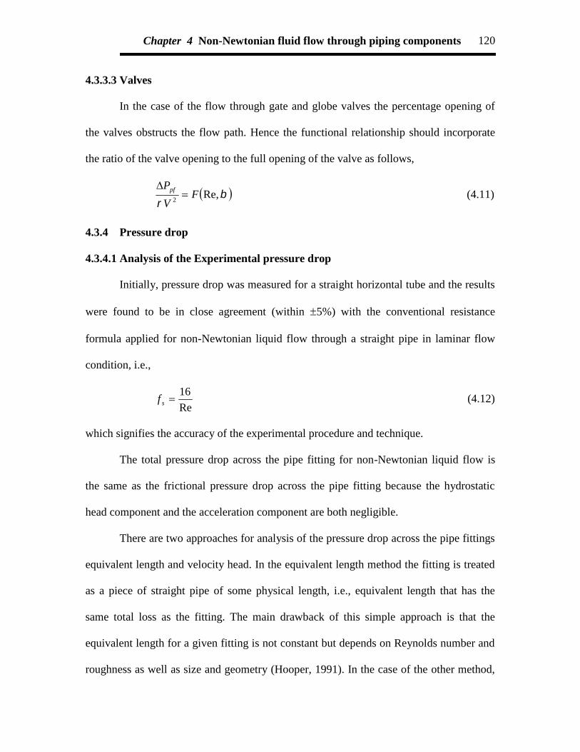
Chapter 4 Non-Newtonian fluid flow through piping components 120
4.3.3.3 Valves
In the case of the flow through gate and globe valves the percentage opening of
the valves obstructs the flow path. Hence the functional relationship should incorporate
the ratio of the valve opening to the full opening of the valve as follows,
Re,2
FV
Ppf
(4.11)
4.3.4 Pressure drop
4.3.4.1 Analysis of the Experimental pressure drop
Initially, pressure drop was measured for a straight horizontal tube and the results
were found to be in close agreement (within 5%) with the conventional resistance
formula applied for non-Newtonian liquid flow through a straight pipe in laminar flow
condition, i.e.,
Re
16sf (4.12)
which signifies the accuracy of the experimental procedure and technique.
The total pressure drop across the pipe fitting for non-Newtonian liquid flow is
the same as the frictional pressure drop across the pipe fitting because the hydrostatic
head component and the acceleration component are both negligible.
There are two approaches for analysis of the pressure drop across the pipe fittings
equivalent length and velocity head. In the equivalent length method the fitting is treated
as a piece of straight pipe of some physical length, i.e., equivalent length that has the
same total loss as the fitting. The main drawback of this simple approach is that the
equivalent length for a given fitting is not constant but depends on Reynolds number and
roughness as well as size and geometry (Hooper, 1991). In the case of the other method,

Chapter 4 Non-Newtonian fluid flow through piping components 121
the velocity head is the amount of potential energy (head) necessary to accelerate a fluid
to its flowing velocity. The number of velocity head (H) in a flowing fluid can be
calculated directly from the velocity of the fluid (V) as
g
VH
2
2
(4.13)
Flow through a piping component in a pipeline also cause a reduction in static head,
which may be expressed in terms of velocity head and the resistance coefficient, K as,
g
VKH
2
2
(4.14)
Friction losses for fittings are often expressed in terms of the resistance coefficient, K. It
can be shown, using dimensional analysis, that for incompressible fluids K is a
dimensionless function of Reynolds number and of dimensionless geometric ratios
characteristic of the fitting. Figs 4.11 - 4.14 illustrate the comparison between the
experimental values and the correlations available in the literature in terms of the
resistance coefficient. It is clear from these figures that the experimental data deviates
from the correlations available in the literature. These differences are attributed by the
size of pipe fittings, rheological behaviour of the liquid, the circuit employed in
transporting the liquid and so-called “mutual influence effect” of the pipe fittings
(Bandala-Rocha et al., 2005). So the analysis of the experimental pressure drop data
across the pipefitting is carried out by means of dimensional analysis. Parameters
influencing the friction loss or pressure drop are the physical and operating variables of
the system. The physical variables include the radius of the tube, the characteristics
dimension of the piping component (radius of curvature of the elbow, percentage opening
of the valves and the orifice etc) and the physical properties of the fluid. However, the

Chapter 4 Non-Newtonian fluid flow through piping components 122
operating variables are limited to the flow rate of the fluid. The final generalized
correlations for the different pipe fittings are given below,
Elbows
519.0718.02
1351094.71
DeX
f
f
s
pf (4.15)
for, 40 Re 2200
30 De 2150
45o 135o
Gate valve
987.1197.02
Re905.1
V
Ppf (4.16)
for, 45 Re 2200
0.25 1.0
Globe valve
797.0061.02
Re266.8
V
Ppf (4.17)
for, 45 Re 2200
0.25 1.0
Orifice
379.4
0048.02
Re601.0
t
pf
D
D
V
P
(4.18)
for, 45 Re 2200
0.4646 D0/Dt 0.7087

Chapter 4 Non-Newtonian fluid flow through piping components 123
4.3.4.2 Stream-wise pressure drop due to piping components
To determine the pressure drop across the fitting, the static pressure was measured
in the long upstream and long downstream portion of the fitting. The static pressure starts
to deviates from the steady value within 5 to 8 (5 for elbow and 8 for globe valve) pipe
diameter of the inlet of the pipefitting and the pressure recovery lengths were also found
to be within 5 to 8 (5 for elbow and 8 for globe valve) pipe diameter.
4.4 Conclusions
Experimental investigations have been carried out to evaluate the pressure drop
across the piping components for non-Newtonian pseudoplastic liquid flow in laminar
condition.
Generalized empirical correlations have been developed to predict the frictional
pressure drop across the different pipe fittings in the horizontal plane, for non-Newtonian
pseudo plastic liquid in laminar flow.
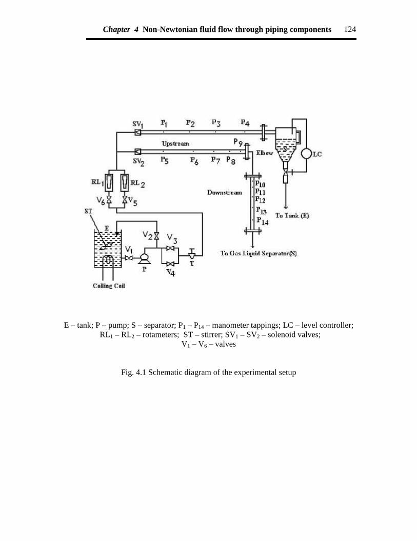
Chapter 4 Non-Newtonian fluid flow through piping components 124
E – tank; P – pump; S – separator; P1 – P14 – manometer tappings; LC – level controller;RL1 – RL2 – rotameters; ST – stirrer; SV1 – SV2 – solenoid valves;
V1 – V6 – valves
Fig. 4.1 Schematic diagram of the experimental setup

Chapter 4 Non-Newtonian fluid flow through piping components 125
Fig. 4.2 Static pressure distribution curve across the valve
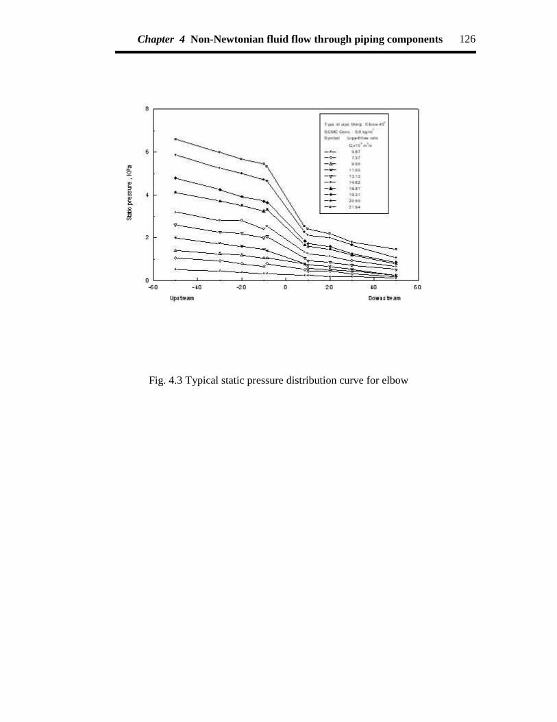
Chapter 4 Non-Newtonian fluid flow through piping components 126
Fig. 4.3 Typical static pressure distribution curve for elbow
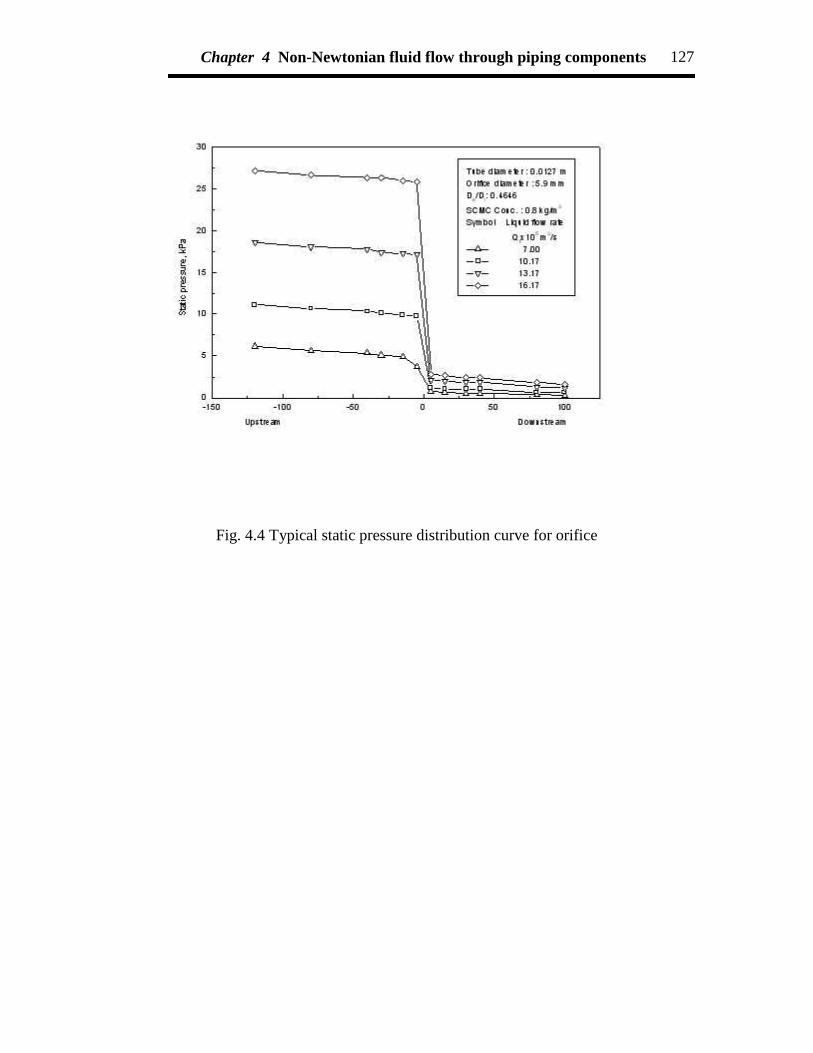
Chapter 4 Non-Newtonian fluid flow through piping components 127
Fig. 4.4 Typical static pressure distribution curve for orifice

Chapter 4 Non-Newtonian fluid flow through piping components 128
Fig. 4.5 Typical static pressure distribution curve for gate valve
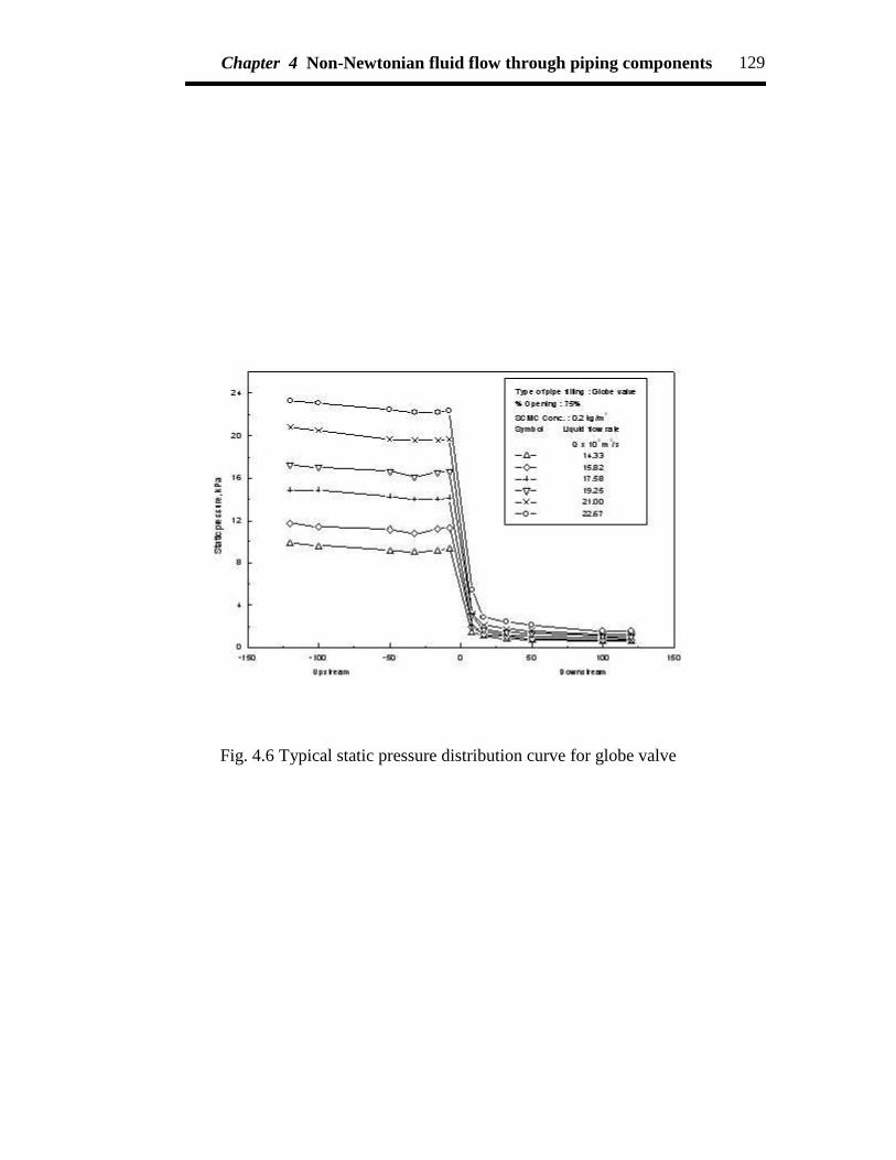
Chapter 4 Non-Newtonian fluid flow through piping components 129
Fig. 4.6 Typical static pressure distribution curve for globe valve

Chapter 4 Non-Newtonian fluid flow through piping components 130
Fig. 4.7 Variation of the pressure drop across the elbow with liquid flow rate

Chapter 4 Non-Newtonian fluid flow through piping components 131
Fig. 4.8 Variation of the pressure drop across the orifice with liquid flow rate

Chapter 4 Non-Newtonian fluid flow through piping components 132
Fig. 4.9 Variation of the pressure drop across the gate valve with liquid flow rate

Chapter 4 Non-Newtonian fluid flow through piping components 133
Fig. 4.10 Variation of the pressure drop across the globe valve with liquid flow rate
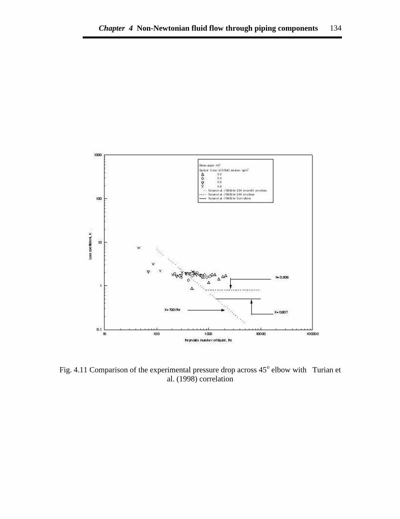
Chapter 4 Non-Newtonian fluid flow through piping components 134
Fig. 4.11 Comparison of the experimental pressure drop across 45o elbow with Turian etal. (1998) correlation
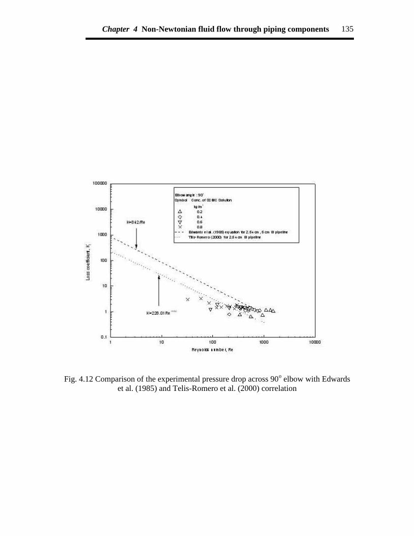
Chapter 4 Non-Newtonian fluid flow through piping components 135
Fig. 4.12 Comparison of the experimental pressure drop across 90o elbow with Edwardset al. (1985) and Telis-Romero et al. (2000) correlation

Chapter 4 Non-Newtonian fluid flow through piping components 136
Fig. 4.13 Comparison of the experimental pressure drop across gate valve with Edwardset al. (1985) and Turian et al. (1998) correlation
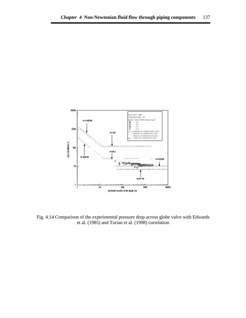
Chapter 4 Non-Newtonian fluid flow through piping components 137
Fig. 4.14 Comparison of the experimental pressure drop across globe valve with Edwardset al. (1985) and Turian et al. (1998) correlation

Chapter 4 Non-Newtonian fluid flow through piping components 138
Table 4.1 Dimension of the piping components
Type of pipe fitting : ElbowElbow angle deg.
Radius of curvatureRc, m
Linear length of the elbowL, m
45 0.011 0.01490 0.022 0.011
135 0.017 0.016Type of pipe fitting : Orifice
Orifice diameterD0, mm
Ratio of orifice diameter to pipe diameterD0/Dt
5.9 0.46467.6 0.59849.0 0.7087
Table 4.2 Physical properties of the SCMC solution
Concentration
3kgm
Flow behaviourindex
n/
Consistency indexK/
2/ mNs n
Density
l
3kgm0.2 0.9013 0.0142 1001.690.4 0.7443 0.1222 1002.130.6 0.6605 0.3416 1002.370.8 0.6015 0.7112 1003.83
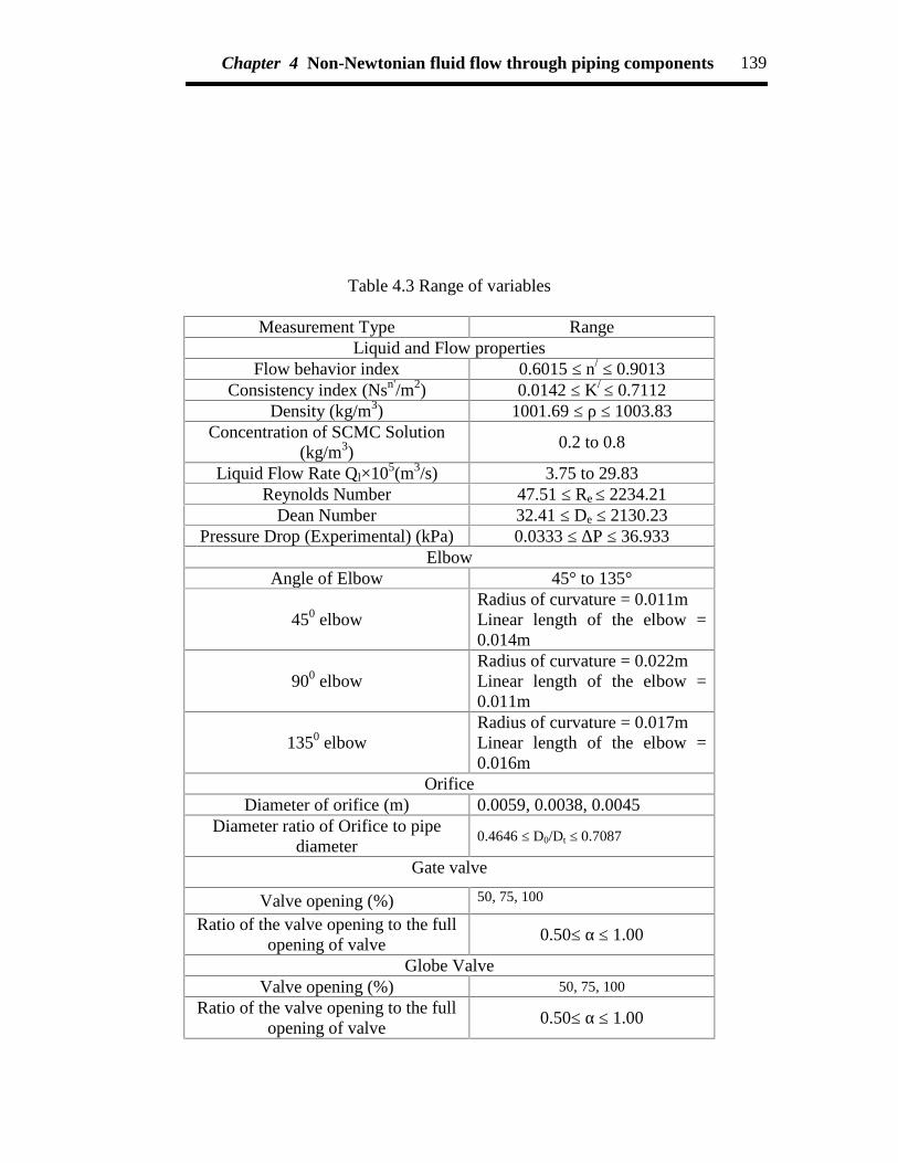
Chapter 4 Non-Newtonian fluid flow through piping components 139
Table 4.3 Range of variables
Measurement Type RangeLiquid and Flow properties
Flow behavior index 0.6015 ≤ n/ ≤ 0.9013Consistency index (Nsn'/m2) 0.0142 ≤ K/ ≤ 0.7112
Density (kg/m3) 1001.69 ≤ ρ ≤ 1003.83Concentration of SCMC Solution
(kg/m3)0.2 to 0.8
Liquid Flow Rate Ql×105(m3/s) 3.75 to 29.83Reynolds Number 47.51 ≤ Re ≤ 2234.21
Dean Number 32.41 ≤ De ≤ 2130.23Pressure Drop (Experimental) (kPa) 0.0333 ≤ ΔP ≤ 36.933
ElbowAngle of Elbow 45° to 135°
450 elbowRadius of curvature = 0.011mLinear length of the elbow =0.014m
900 elbowRadius of curvature = 0.022mLinear length of the elbow =0.011m
1350 elbowRadius of curvature = 0.017mLinear length of the elbow =0.016m
OrificeDiameter of orifice (m) 0.0059, 0.0038, 0.0045
Diameter ratio of Orifice to pipediameter
0.4646 ≤ D0/Dt ≤ 0.7087
Gate valve
Valve opening (%) 50, 75, 100
Ratio of the valve opening to the fullopening of valve
0.50≤ α ≤ 1.00
Globe ValveValve opening (%) 50, 75, 100
Ratio of the valve opening to the fullopening of valve
0.50≤ α ≤ 1.00

Chapter 4 Non-Newtonian fluid flow through piping components 140

Chapter 5
Non-Newtonian liquid flow through small diameter pipingcomponents – CFD analysis

Chapter 5 Non-Newtonian liquid flow through ----- CFD analysis 141
Computational Fluid Dynamics (CFD) analysis have been carried out to evaluate
the frictional pressure drop across the horizontal pipeline and different piping
components, like elbows, orifices, gate and globe valves for non-Newtonian liquid
through 0.0127m pipe line. The mesh generation is done using Gambit 6.3 and FLUENT
6.3 is used for CFD analysis. The CFD results show the very good agreement with the
experimental values.
5.1 Introduction
The integral part of any piping systems are valves, bends, elbows, orifices, tees,
reducers, expander etc. Flow through piping components is more complex than the
straight pipes. The complex nature arises due to the presence of constriction and
expansion, change of flow direction etc. Consumption of energy across pipe fittings gives
pressure losses which expressed as a pressure drops. The friction between the fluid and
the fitting wall causes this pressure drop. Pressure drop across the pipe fittings is
important in design and analysis of the fluid machinery. Process engineers are dealing
with non-Newtonian fluids mainly in food processing, paints, pharmaceutical, paper, and
petroleum industry for production and transportation of foods, paints, glues, colors, fiber
solutions, polymer solutions through piping components.
Computational Fluid Dynamics (CFD) can serve to evaluate the frictional losses
in piping systems, secondary flow effects can be visualized to aid in better understanding
of the flow phenomena and can be applied to improve flow characteristics and equipment
design. However CFD analysis often requires fine tuning by comparison with the reliable
experimental data. CFD is a useful tool for studying non-Newtonian flows. The
improvements in computer performance, matched by the developments in numerical

Chapter 5 Non-Newtonian liquid flow through ----- CFD analysis 142
methods, have resulted in a growing confidence in the ability of CFD to model complex
fluid flows. CFD techniques have been used on a broad scale in the process industry to
gain insight into various flow phenomena, examine different equipment designs or
compare performance under different operating conditions (Abbott and Basco, 1989, Xia
and Sun, 2002). The use of viscous non-Newtonian fluids in industry poses a number of
challenges. Highly viscous fluids require much energy to flow in pipelines and
processing equipments.
Numerical simulation of gas-solid flow in a U-bend was reported by Hidayat and
Rasmuson (2002). Etemad and Sunden (2004) studied numerical analysis of turbulent
convective heat transfer in a square–sectioned U-bend duct. Marn and Ternik (2006)
numerically studied laminar flow of shear-thickening electrostatic ash-water mixture
through 90o pipe bend. Edwards et al. (1998) developed a CFD based model to predict
erosion in piping system in slurry pipeline. Numerical simulations are performed for the
dilute gas-solid flow through rectangular duct containing a horizontal to vertical bend of
90o angle by Kuan et al. (2003). Brown (2006) has been used to investigate the cause of
highly localized erosion in slurry pipeline in an aluminium refinery through CFD and
subsequently used for the development of the newer pipeline. Saha and Jain (2008) used
CFD analysis for slurry pipeline to investigate the erosion in the pipeline. Wu and Chen
(2008) used commercial CFD code to simulate the flow fields of lab-scale, scale-up and
pilot-scale anaerobic digesters. Their simulated results were validated against the
experimental data from literature using liquid as Newtonian and non-Newtonian in
nature. Manzar and Shah (2009) reported the CFD analysis for straight and coils tubes
using different Newtonian and non-Newtonian liquids.

Chapter 5 Non-Newtonian liquid flow through ----- CFD analysis 143
The CFD has been used for many steady flow engineering devices such as pipe
junction (Sierra-Espinosa et al., 2000a and b), pipeline design (Famiyesin et al., 2002)
etc. The use of CFD to study the effect of modifying valve geometry on flow
characteristics is also very important in valve design and performance. Roorda (1998)
and Davis and Stewart (1998) reported their work on this direction for the control valve
design. In any use of CFD for improving component design, it is vital that suitable
validation studies be undertaken.
In this paper, the CFD modeling of the hydrodynamics of non-Newtonian flow
through straight pipe, elbows, orifices, gate and globe valves are described. The Fluent
6.3 is used as CFD code. The applicability of the Fluent 6.3 software in the flow of non-
Newtonian liquid through small diameter pipeline and the piping components are
investigated. The numerical results are compared with the results as shown in Chapter 4.
5.2 Experimental
The detail experimental set up, techniques and results are given in Chapter 4.
5.3 Mathematical Model
The detailed mathematical methods used for the CFD analysis is given in Chapter
2. Dilute solution of SCMC follows the non-Newtonian pseudoplastic Power law model.
In general for non-Newtonian liquids the effective viscosity is used for calculation and
defined as,
1/
/
8
n
eff d
vK (5.1)
The governing equation is the Navier – Stokes equation as,
Pvvvt
veff
2. (5.2)

Chapter 5 Non-Newtonian liquid flow through ----- CFD analysis 144
and the continuity equation is
0v (5.3)
where,z
ky
jx
i
(5.4)
As the flow of liquid is laminar in all cases the viscous model, i.e., laminar non-
Newtonian Power Law model is used for the CFD analysis. These equations are solved
subject to the following boundary conditions,
(i) The pipeline and piping components walls are assumed rigid and a no-slip
condition is imposed.
(ii) At the outlet, the velocities are free but the normal and tangential stresses are
constrained to be zero and the gauge pressure is set to zero.
(iii) At the inlet, a uniform velocity profile is used with a time varying forcing
function representive of flow in the left portion of the piping components.
5.4 Computational fluid dynamics (CFD) Procedure
Geometries for the straight pipe, elbows, orifices, valves and are created in
Gambit 6.3 preprocessor. A typical mesh has about 3x10³ – 2x10⁵ order unstructured
tetrahedral mesh for elbows and unstructured boundary layer hexahedral mesh for
straight pipe, orifices and valves are used. Inlet and outlet are located at each end of the
piping system. The inlet is used to specify the inlet velocity and outlet is used to specify
pressure outlet. These geometries of the pipeline and piping components are imported
into Fluent 6.3 in a Cartesian co-ordinate system. Fluent 6.3 solved the governing
equations in 3-D geometry. Laminar non-Newtonian Power Law model have been used
for simulation. The model solves for Navier-stokes equation at prescribes velocities. The
governing equations are non linear and several iterations of loop must be performed

Chapter 5 Non-Newtonian liquid flow through ----- CFD analysis 145
before a convergent solution is obtained. The first-order upwind scheme is used in the
discretization of set of governing equations, standard interpolation schemes is used for
calculating cell-face pressures for using the Segregated solver in Fluent 6.3. Pressure-
velocity coupling refers to the numerical algorithm which uses a combination of
continuity and momentum equations to derive an equation for pressure (or pressure
correction) when using the segregated solver. Simple algorithm is used in Fluent 6.3
domain.
The general procedure to simulate SCMC flow through pipe and different piping
components based on Gambit 6.3 and Fluent 6.3 software is outlined below,
1. Perform meshing under Gambit 6.3 :
Create a computational domain at the flow region,
The grids were generated using boundary layer hexahedral and t-grid
(tetrahedral) meshes,
Controlling a smooth change in the mesh size by size functions,
Specify boundary and continuum types,
Examine the mesh to ensure that the high skewness is below 0.5 for
hexahedral and below 0.9 for tetrahedral meshes.
2. Import the mesh file to Fluent 6.3 and check the mesh.
3. Define a 3-D, unsteady, implicit, and pressure-based solver.
4. Activate the single phase laminar non-Newtonian power law model.
5. Define a laminar non-Newtonian power law model.
6. Enable the liquid properties with laminar flow conditions using the text
command: define/models/viscous/laminar. Putting the non-Newtonian fluid

Chapter 5 Non-Newtonian liquid flow through ----- CFD analysis 146
values: flow behavior index, consistency index, temperature and effective
viscosity values at the inlet velocity.
7. Define the phase by setting liquid as the single phase. Define the operating
conditions by turning on gravity and specify the operating density.
8. Solution control methodology – Under relaxation factors – 0.5 for pressure, 0.3
for momentum, and default values for the other parameters. Standard schemes –
STANDARD for momentum and 1st order upwind for other variables. Pressure-
velocity SIMPLE coupling used;
9. Initialize the solution – velocity;
Enable the plotting of residuals during the calculation, and kept the default
convergence criteria, 1 X 10⁻⁵ for all residuals except for the transport equation
which residual was set at 10-3.
5.5 Results and discussion
5.5.1Convergence and grid independency
The convergence criterions were set at 10-5 for all equations except for the
transport equation which residual was set at 10-3. A computational domain L≥200D was
used to ensure fully developed flow results could be obtained for all pipe and piping
components. In general the final results depend upon mesh geometries. Subsequent
decrement and increment in mesh resolution by 50% were applied to evaluate if the
employed mesh resolution was adequate to obtain accurate solutions. It was observed that
when the mesh resolution was decreased by 50% the axial velocity profile was 7-12% of
the currently employed mesh velocity profile for pipe and different piping components.
As the present mesh resolution was increased by 50% the axial velocity profile changes

Chapter 5 Non-Newtonian liquid flow through ----- CFD analysis 147
1-3% for pipe and different piping components. These results suggest that the current
mesh resolution is sufficient to obtained grid independent solutions for the proposed
model.
5.5.2 Straight pipe
Boundary layer and hexahedral mesh is fitted with the geometry of pipe as shown
in Fig. 5.1. Fig. 5.2 shows the contour plot of pressure field for straight pipe. At the inlet
of the pipe pressure is high and gradually decreases at the outlet due to friction with the
top and bottom walls. Fig. 5.3 shows the plot of velocity field for straight pipe. It shows
that at the centre of the pipe velocity is high and at the wall velocity is near to zero. Fig.
5.4 shows the comparison plot of the single-phase pressure drop across the straight pipe
for experimental and CFD analysis and it is clear that these two are matches very well.
5.5.3 Elbows
Fig. 5.5 shows the mesh generated for different elbows. Unstructured t-grid
(tetrahedral) is fitted well for the cases of elbows due to its curved structure. Fig. 5.6
shows that plot of velocity field. Fig. 5.7 shows the vector field inside the different
points. Fig. 5.8 shows that the velocity magnitude inside the different points. Fig. 5.9
shows the plot of X-velocity. Fig. 5.10 shows the contours plot of static pressure. Fig.
5.11 shows the contours plot of static pressure inside the different points. Fig. 5.12 shows
the contours plot of total pressure inside the different points.
As the fluid flows through the straight pipe and then enter into the elbow section,
the pressure which is uniform across the flow in the straight section, must adjust in the
elbow to counter the centrifugal force. The pressure is greatest at the outer wall furthest
from the centre of curvature and least at the inner wall nearest to the centre of curvature.

Chapter 5 Non-Newtonian liquid flow through ----- CFD analysis 148
At the inlet of the elbow a low pressure exists in the inner wall and high pressure exists at
the outer wall, it is clearly indicated in Figs. 5.10 - 5.12. This initial pressure gradient
resulting from the change from straight to curve flow, a cross stream pressure gradient
exists in the elbow, at the elbow inlet the boundary layer on the outer wall experiences
the effect of an the adverse stream wise pressure gradient which may be sufficiently
strong for 450 elbow than compare to 1350 elbow and produce local separation and the
inner wall boundary layer is accelerated (Figs. 5.6 - 5.8). The reverse occurs at the exit of
the elbow where local pressure gradients of the opposite sign appear as the flow adjust to
uniform pressure condition of the downstream. The impacts of the curve geometry into
the straight section were extended 5 pipe diameter upstream of the elbow and also 5 pipe
diameter downstream of the elbow. This impacts depends on the velocity of the flow and
also the elbow angle and effect is maximum for the 450 elbow and minimum for the 1350
elbow. Thus the flow at the entrance of the elbow differs considerably from a fully
developed pipe flow. The flow in elbow is influenced by centrifugal force due to its
curvature. This centrifugal force is, in principle, balanced by a pressure gradient in the
plane of curvature. However, near the wall where the velocity is small, this pressure
gradient can no longer be balanced and consequently fluid in the middle of the pipe
moves at the outer wall and then turns to move inward along the wall. The flow on the
outer wall and separation at the inner wall make flow very complex (Fig. 5.9). The result
is a secondary flow superimposed in the main flow in the plane perpendicular to the main
flow. The magnitude and direction of the flow depends on Dean number. The direct
effect of secondary flow is to displace the region of maximum velocity to the centre
towards the outer wall as it is shown in Figs. 5.6 - 5.7. For the elbow entrance the mean

Chapter 5 Non-Newtonian liquid flow through ----- CFD analysis 149
axial velocity profile significantly altered with respect to the fully developed profile in
the straight pipe and the location of the maximum velocity is shifted towards the inner
wall of the elbow, as shown in Figs. 5.6 - 5.8. This explained by the fact that no
centrifugal forces due to redirection of flow are present at the entrance of the flow.
The flow in 900 elbow is always developing in nature in which the velocity
distribution do not attain other forms that are more or less independent of the position
along the pipe axis. For 450 elbow exist the axial velocity moves further towards the outer
radius as clearly shown in Figs. 5.6 - 5.7. The secondary motion can be seen clearly in the
Fig. 5.9. At the elbow entrance the centrifugal forces are very weak to balance the
pressure gradient which results in an inward flow as shown in Figs. 5.6 – 5.7. With
increasing deflection that is flow through inside the elbows the centrifugal forces
increases and counter rotating vortices that circulate in the outer direction in the central
part of the pipe. This is shown in Fig. 5.9. It is more pronounced in the 450 elbow than
other elbows. As the flow passes to the elbow this vortices shifted towards the inner wall
(Fig. 5.9) and then the static pressure starts to deviate from steady value within 15 pipe
diameter in the upstream of the inlet of the elbows, depending on the flow rate. In the
downstream of the elbow, the pressure recovery lengths were found to be within 20 pipe
diameter for all elbows, depending on the flow rate. Similar results are obtained by Kuan
et al. (2003), Berrouk and Laurence (2008), Kumar et al. (2008) and Zhang et al. (2010).
Figs. 5.13 - 5.14 show the comparison plot of the pressure drop across the elbows
for experimental and CFD analysis. It is clear from the figure that the non-Newtonian
liquid flow through elbows, the experimental pressure drop data matches well with the
CFD simulated results.

Chapter 5 Non-Newtonian liquid flow through ----- CFD analysis 150
5.5.4 Orifices
Boundary layer and hexahedral mesh is fitted well with the geometry of the
orifice (Fig. 5.15). Fig. 5.16 shows the contour plot of pressure field of the orifice and
Fig. 5.17 shows the contour plot of static pressure at different points of the orifice.
Similar plot observed for the case of other orifices. It shows that flow through orifices,
the sudden reduction of the flow path is followed by re-establishment of the flow path.
The velocity is a maximum near the orifice. According to Bernoulli’s principle, this
region of high velocity is also a region of low pressure. Hence the pressure, shear stress
and shear strain increases with increasing the flow area with increasing the diameter ratio,
D0/Dt. Pressure drop decreases with increasing the diameter ratio, D0/Dt. Fig. 5.18 shows
the plot of velocity vector field of the orifice. Fig. 5.19 shows the plot of velocity vector
field at the different points of the orifice. Fig. 5.20 shows the plot of velocity magnitude
at the different points of the orifice. Similar plot observed for the case of other orifices. It
shows that due to gradual decreasing of D0/Dt ratio from 0.7087 to 0.4646, i.e., narrowing
of flow area velocity is increased. Figs. 5.21 - 22 shows the comparison plot of the
pressure drop across the orifices for experimental and CFD analysis. Results are matches
well.
5.5.5 Gate valve
Fig. 5.23 shows that boundary layer hexahedral mesh for 50% opening gate valve.
The valve is drawn is somewhat simplified manner with intact it internal dimensions. Fig.
5.24 shows that contour plot of static pressure and Fig. 5.25 shows that contour plot of
total pressure for 50% opening gate valve. The contour plot of pressure field shows that
the pressure drop decreases with increasing the percentage opening of the valve. The

Chapter 5 Non-Newtonian liquid flow through ----- CFD analysis 151
shear strain and shear stress gradually decreases with increase in flow area, i.e.,
percentage opening of the valve. The pressure drop increases with increasing liquid
concentration, i.e., pseudoplasticity of the liquid at constant liquid flow rate. Figs. 5.26
and 5.27 show that plot of velocity magnitude and velocity vector field. The velocity is
increases due to the presence of orifice, i.e., by decreasing the flow area, and again
reestablished the lower velocity. Figs. 5.28 - 5.29 show that comparison plot of the
pressure drop across the gate valves for experimental and CFD analysis. It is clear from
the figure that pressure drop matches well. However the simplified figure has drawn for
meshing due to the large pressure drop experimental and CFD data matches well
5.5.6 Globe valve
Boundary layer and hexahedral mesh is fitted well with the geometry of Globe
Valve. Fig. 5.30 shows the mesh geometry of the globe valve and the geometry are
simplified with intact its entire internal dimension. The pressure drop across the valve
behaves similar to the gate valve, but only different is a change in the flow direction
occurs. Fig. 5.31 shows the plot of velocity field. The change of flow direction is clearly
observed in the figure. Figs. 5.32 - 5.33 show the comparison plot which gives good
agreement with the CFD simulated values, but differ slightly and it may be due to its
simplified geometry taken in this studies.
5.6 Conclusions
Commercially available software FLUENT 6.3 was used to calculate pressure
drops in pipeline and piping components for non-Newtonian liquid flow. The numerical
simulated results are verified with experimental data and it gives excellent agreement.
The numerical simulated results also provide detail information of the flow field in

Chapter 5 Non-Newtonian liquid flow through ----- CFD analysis 152
pipeline and piping components. It gives better physical insights and understanding of the
flow phenomena. This study demonstrated the Computational fluid dynamics (CFD)
application as an effective tool for design in the pipeline and piping components.
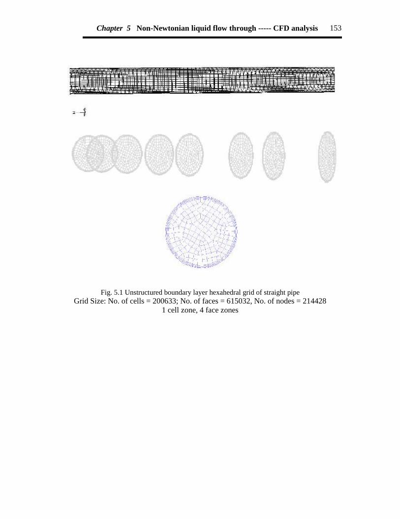
Chapter 5 Non-Newtonian liquid flow through ----- CFD analysis 153
Fig. 5.1 Unstructured boundary layer hexahedral grid of straight pipeGrid Size: No. of cells = 200633; No. of faces = 615032, No. of nodes = 214428
1 cell zone, 4 face zones
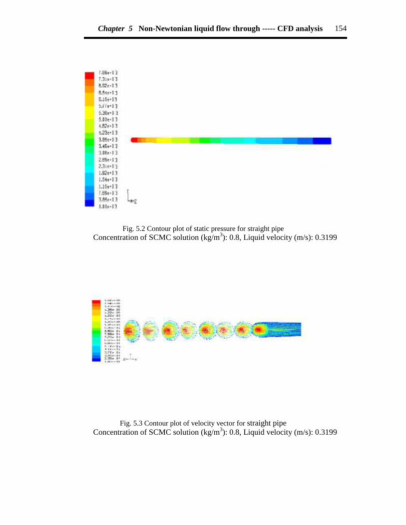
Chapter 5 Non-Newtonian liquid flow through ----- CFD analysis 154
Fig. 5.2 Contour plot of static pressure for straight pipeConcentration of SCMC solution (kg/m3): 0.8, Liquid velocity (m/s): 0.3199
Fig. 5.3 Contour plot of velocity vector for straight pipeConcentration of SCMC solution (kg/m3): 0.8, Liquid velocity (m/s): 0.3199

Chapter 5 Non-Newtonian liquid flow through ----- CFD analysis 155
0.2 0.4 0.6 0.8 1.0 1.2 1.41
2
3
4
5
6
7
8
9
Pres
sure
dro
p, k
Pa
Liquid velocity, m/s
Symbol Type SCMC Conc. kg/m3
Expt. 0.8 CFD 0.8 Expt. 0.6 CFD 0.6 Expt. 0.4 CFD 0.4
Fig. 5.4 Comparison of the experimental data and CFD modeling for straight pipe

Chapter 5 Non-Newtonian liquid flow through ----- CFD analysis 156
(a) (b)
(c)
Fig. 5.5 Mesh geometry - Unstructured Tetrahedral grid(a) 450 elbow
Grid Size: No. of cells = 25985; No. of faces = 57149, No. of nodes = 73101 cell zone, 4 face zones
(b) 900 elbowGrid Size: No. of cells = 29157; No. of faces = 64167, No. of nodes = 8208
1 cell zone, 4 face zones(c) 135 0 elbow
Grid Size: No. of cells = 4427; No. of faces = 9778, No. of nodes = 12791 cell zone, 4 face zones

Chapter 5 Non-Newtonian liquid flow through ----- CFD analysis 157
(a) (b)
(c)
Fig. 5.6 Plot of velocity vector(a) 450 elbow
Concentration of SCMC solution (kg/m3): 0.2, Liquid velocity (m/s): 0.296(b) 90 0 elbow
Concentration of SCMC solution (kg/m3): 0.2, Liquid velocity (m/s): 0.296(c) 135 0 elbow
Concentration of SCMC solution (kg/m3): 0.8, Liquid velocity (m/s): 1.733

Chapter 5 Non-Newtonian liquid flow through ----- CFD analysis 158
Fig. 5.7a Contours plot of velocity vector inside the different points of 450 elbowConcentration of SCMC solution (kg/m3): 0.8, Liquid flow rate, Ql (m
3/s): 21.94x10⁻⁵

Chapter 5 Non-Newtonian liquid flow through ----- CFD analysis 159
Fig. 5.7b Contour plot of velocity vector inside the different points of 900 elbowConcentration of SCMC solution (kg/m3): 0.8, Liquid flow rate, Ql (m
3/s): 21.94x10⁻⁵, Liquidvelocity, Vl (m/s): 1.733
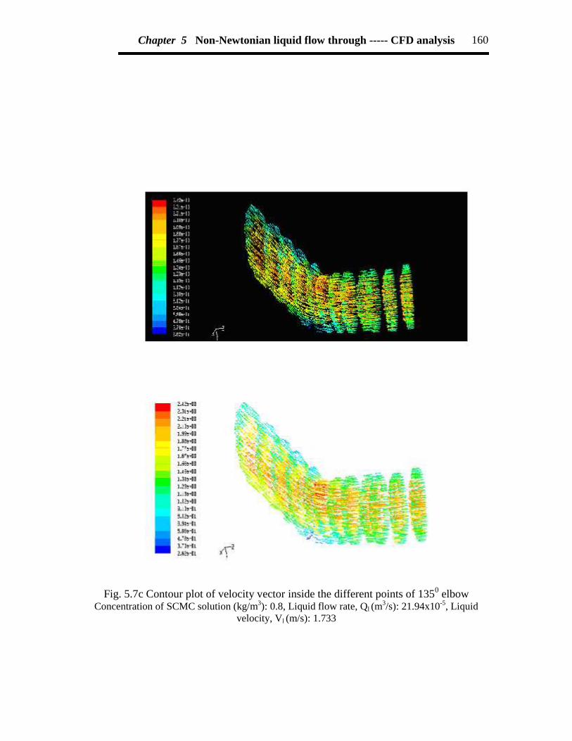
Chapter 5 Non-Newtonian liquid flow through ----- CFD analysis 160
Fig. 5.7c Contour plot of velocity vector inside the different points of 1350 elbowConcentration of SCMC solution (kg/m3): 0.8, Liquid flow rate, Ql (m
3/s): 21.94x10⁻⁵, Liquidvelocity, Vl (m/s): 1.733

Chapter 5 Non-Newtonian liquid flow through ----- CFD analysis 161
Fig. 5.8a Contours plot of velocity magnitude inside the different points of 450 elbow,Concentration of SCMC solution (kg/m3): 0.8, Liquid flow rate, Ql (m
3/s): 21.94x10⁻⁵, Liquidvelocity, Vl (m/s): 1.733

Chapter 5 Non-Newtonian liquid flow through ----- CFD analysis 162
Fig. 5.8b Contour plot of velocity magnitude inside the different points of 900 elbow

Chapter 5 Non-Newtonian liquid flow through ----- CFD analysis 163
Concentration of SCMC solution (kg/m3): 0.8, Liquid flow rate, Ql (m3/s): 21.94x10⁻⁵, Liquid
velocity, Vl (m/s): 1.733
Fig. 5.8c Contour plot of velocity magnitude inside the different points of 1350 elbow,Concentration of SCMC solution (kg/m3): 0.8, Liquid flow rate, Ql (m
3/s): 21.94x10⁻⁵, Liquidvelocity, Vl (m/s): 1.733
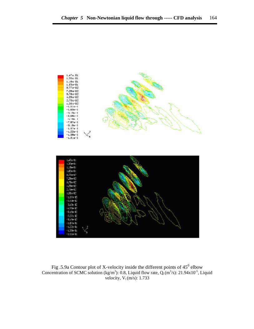
Chapter 5 Non-Newtonian liquid flow through ----- CFD analysis 164
Fig .5.9a Contour plot of X-velocity inside the different points of 450 elbowConcentration of SCMC solution (kg/m3): 0.8, Liquid flow rate, Ql (m
3/s): 21.94x10⁻⁵, Liquidvelocity, Vl (m/s): 1.733

Chapter 5 Non-Newtonian liquid flow through ----- CFD analysis 165
Fig. 5.9b Contour plot of X-velocity inside the different points of 900 elbowConcentration of SCMC solution (kg/m3): 0.8, Liquid flow rate, Ql (m
3/s): 21.94x10⁻⁵, Liquidvelocity, Vl (m/s): 1.733
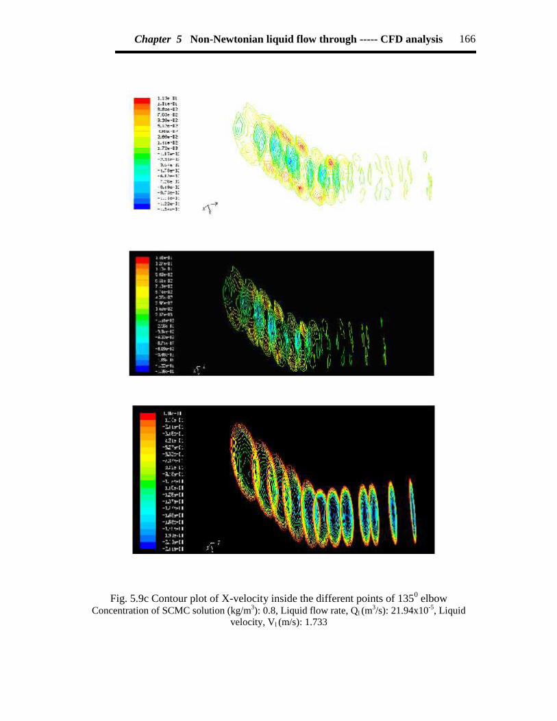
Chapter 5 Non-Newtonian liquid flow through ----- CFD analysis 166
Fig. 5.9c Contour plot of X-velocity inside the different points of 1350 elbowConcentration of SCMC solution (kg/m3): 0.8, Liquid flow rate, Ql (m
3/s): 21.94x10⁻⁵, Liquidvelocity, Vl (m/s): 1.733
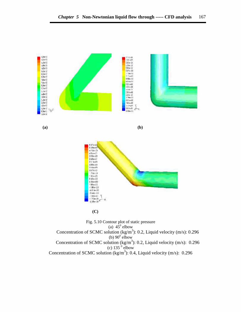
Chapter 5 Non-Newtonian liquid flow through ----- CFD analysis 167
(a) (b)
(C)
Fig. 5.10 Contour plot of static pressure(a) 450 elbow
Concentration of SCMC solution (kg/m3): 0.2, Liquid velocity (m/s): 0.296(b) 900 elbow
Concentration of SCMC solution (kg/m3): 0.2, Liquid velocity (m/s): 0.296(c) 135 0 elbow
Concentration of SCMC solution (kg/m3): 0.4, Liquid velocity (m/s): 0.296
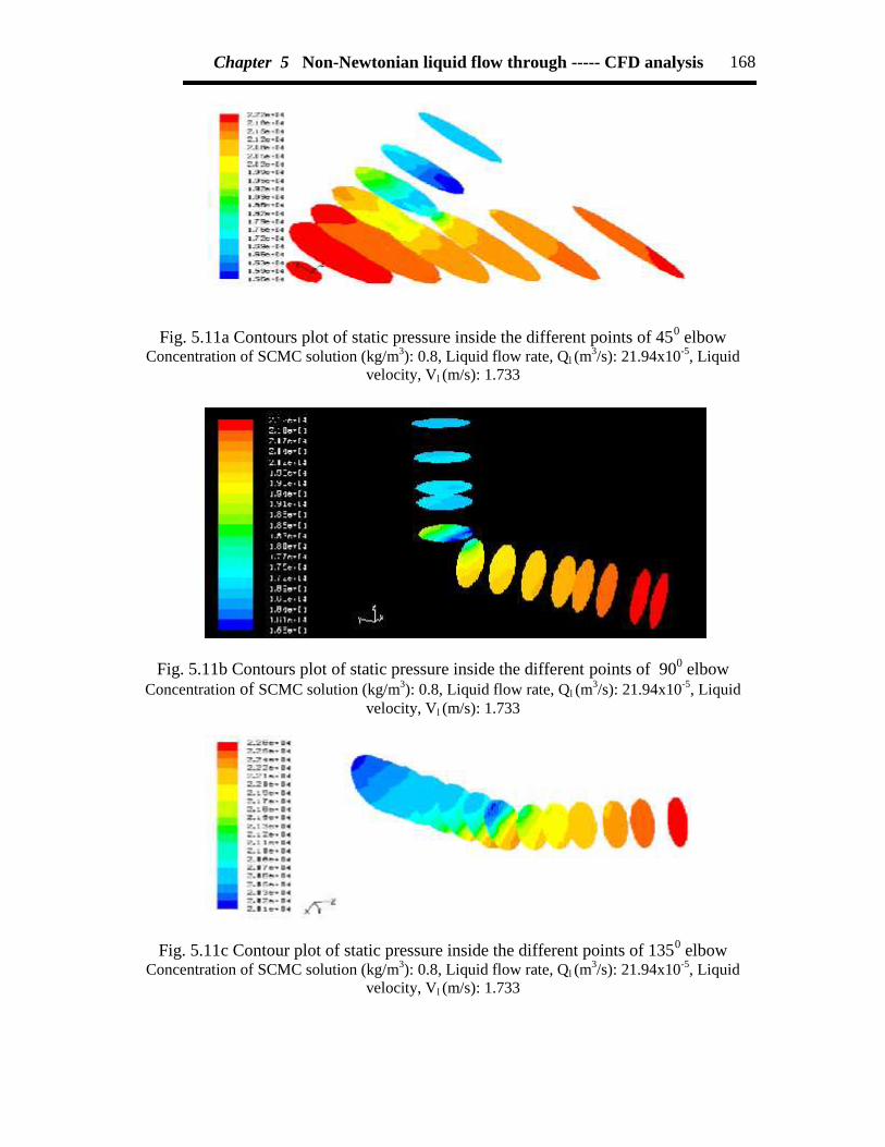
Chapter 5 Non-Newtonian liquid flow through ----- CFD analysis 168
Fig. 5.11a Contours plot of static pressure inside the different points of 450 elbowConcentration of SCMC solution (kg/m3): 0.8, Liquid flow rate, Ql (m
3/s): 21.94x10⁻⁵, Liquidvelocity, Vl (m/s): 1.733
Fig. 5.11b Contours plot of static pressure inside the different points of 900 elbowConcentration of SCMC solution (kg/m3): 0.8, Liquid flow rate, Ql (m
3/s): 21.94x10⁻⁵, Liquidvelocity, Vl (m/s): 1.733
Fig. 5.11c Contour plot of static pressure inside the different points of 1350 elbowConcentration of SCMC solution (kg/m3): 0.8, Liquid flow rate, Ql (m
3/s): 21.94x10⁻⁵, Liquidvelocity, Vl (m/s): 1.733

Chapter 5 Non-Newtonian liquid flow through ----- CFD analysis 169
Fig. 5.12a Contour plot of total pressure inside the different points of 450 elbow,Concentration of SCMC solution (kg/m3): 0.8, Liquid flow rate, Ql (m
3/s): 21.94x10⁻⁵,Liquid velocity, Vl (m/s): 1.733
Fig. 5.12b Contour plot of total pressure inside the different points of 1350 elbow,Concentration of SCMC solution (kg/m3): 0.8, Liquid flow rate, Ql (m
3/s): 21.94x10⁻⁵,Liquid velocity, Vl (m/s): 1.733

Chapter 5 Non-Newtonian liquid flow through ----- CFD analysis 170
-60 -40 -20 0 20 40 601
2
3
4
5
6
7
Stat
ic P
resu
ure,
kPa
Upstream Elbow Downstream
Type of pipe fitting: Elbow 450
SCMC Conc.: 0.8 kg/m3
Symbol Type Liquid flow rate Qlx105 m3/s
Expt. 21.94 CFD 21.94 Expt. 20.50 CFD 20.50 Expt. 18.31 CFD 18.31
Fig.5.13 Comparison plot of experimental and CFD for 450 elbow

Chapter 5 Non-Newtonian liquid flow through ----- CFD analysis 171
0.2 0.4 0.6 0.8 1.0 1.2
0.0
0.2
0.4
0.6
0.8
1.0
1.2
Pres
sure
dro
p, k
Pa
Liquid velocity, m/s
Symbol Type Elbow SCMC angle conc. kg/m3
Expt. 450 0.2 CFD 450 0.2 Expt. 900 0.2 CFD 900 0.2 Expt. 1350 0.2 CFD 1350 0.2
Fig. 5.14 Comparison of the experimental data and CFD modeling for elbows
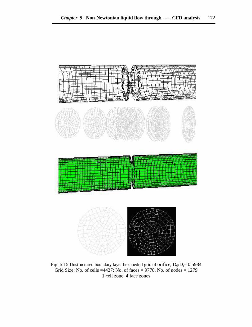
Chapter 5 Non-Newtonian liquid flow through ----- CFD analysis 172
Fig. 5.15 Unstructured boundary layer hexahedral grid of orifice, D0/Dt= 0.5984Grid Size: No. of cells =4427; No. of faces = 9778, No. of nodes = 1279
1 cell zone, 4 face zones
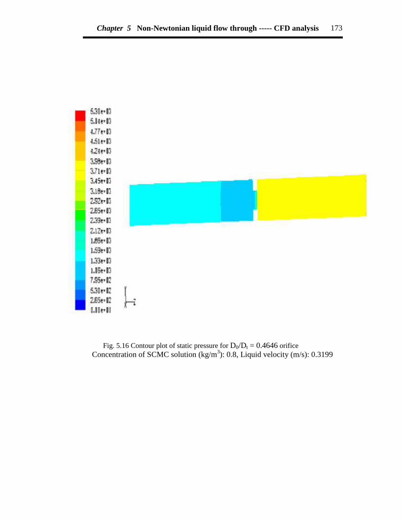
Chapter 5 Non-Newtonian liquid flow through ----- CFD analysis 173
Fig. 5.16 Contour plot of static pressure for D0/Dt = 0.4646 orificeConcentration of SCMC solution (kg/m3): 0.8, Liquid velocity (m/s): 0.3199

Chapter 5 Non-Newtonian liquid flow through ----- CFD analysis 174
Fig. 5.17 Contour plot of static pressure at different points of D0/Dt = 0.5984 orificeConcentration of SCMC solution (kg/m3): 0.8, Liquid velocity (m/s): 1.2772

Chapter 5 Non-Newtonian liquid flow through ----- CFD analysis 175
Fig. 5.18 Plot of velocity vector for D0/Dt = 0.4646 orificeConcentration of SCMC solution (kg/m3): 0.8, Liquid velocity (m/s): 0.3199
Fig. 5.19 Plot of velocity vector at different points of D0/Dt = 0.5984 orificeConcentration of SCMC solution (kg/m3): 0.8, Liquid velocity (m/s): 1.2772
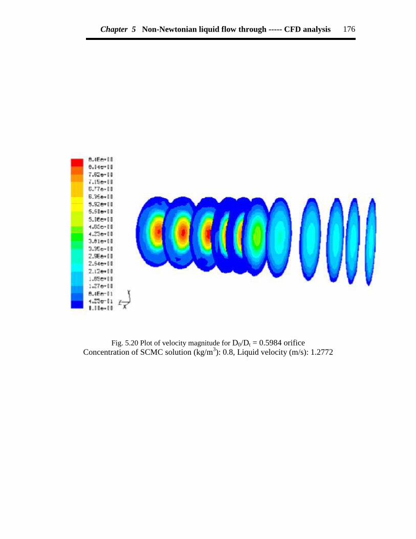
Chapter 5 Non-Newtonian liquid flow through ----- CFD analysis 176
Fig. 5.20 Plot of velocity magnitude for D0/Dt = 0.5984 orificeConcentration of SCMC solution (kg/m3): 0.8, Liquid velocity (m/s): 1.2772
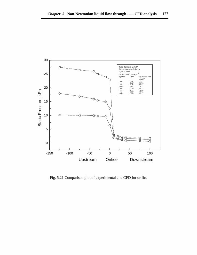
Chapter 5 Non-Newtonian liquid flow through ----- CFD analysis 177
-150 -100 -50 0 50 100
0
5
10
15
20
25
30
Stat
ic P
ress
ure,
kPa
Upstream Orifice Downstream
Tube diameter: 0.0127Orifice diameter: 5.9 mmD
0/D
t: 0.4646
SCMC Conc.: 0.8 kg/m3
Symbol Type Liquid flow rate Q
lx105
Expt. 16.17 CFD 16.17 Expt. 13.17 CFD 13.17 Expt. 10.17 CFD 10.17
Fig. 5.21 Comparison plot of experimental and CFD for orifice

Chapter 5 Non-Newtonian liquid flow through ----- CFD analysis 178
0.5 1.0 1.5 2.0 2.5 3.0 3.5 4.0 4.5 5.00
5
10
15
20
25
Pres
sure
dro
p, k
Pa
Liquid velocity, m/s
Symbol Type Orifice SCMC diameter conc. ratio kg/m3
D0/Dt Expt. 0.4646 0.8 CFD 0.4646 0.8 Expt. 0.5984 0.8 CFD 0.5984 0.8 Expt. 0.7087 0.8 CFD 0.7087 0.8
Fig. 5.22 Comparison of the experimental data and CFD modeling for orifices

Chapter 5 Non-Newtonian liquid flow through ----- CFD analysis 179
Fig. 5.23 Grid for 50% opening gate valve
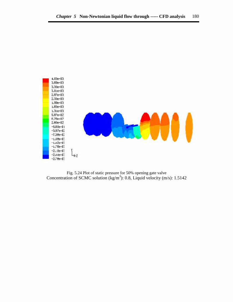
Chapter 5 Non-Newtonian liquid flow through ----- CFD analysis 180
Fig. 5.24 Plot of static pressure for 50% opening gate valveConcentration of SCMC solution (kg/m3): 0.8, Liquid velocity (m/s): 1.5142
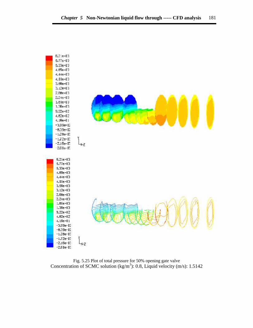
Chapter 5 Non-Newtonian liquid flow through ----- CFD analysis 181
Fig. 5.25 Plot of total pressure for 50% opening gate valveConcentration of SCMC solution (kg/m3): 0.8, Liquid velocity (m/s): 1.5142

Chapter 5 Non-Newtonian liquid flow through ----- CFD analysis 182
Fig. 5.26 Plot of velocity magnitude for 50% opening gate valveConcentration of SCMC solution (kg/m3): 0.8, Liquid velocity (m/s): 1.5142
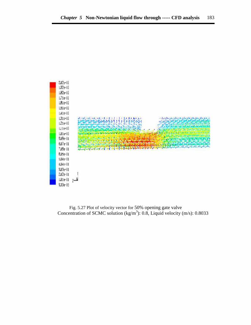
Chapter 5 Non-Newtonian liquid flow through ----- CFD analysis 183
Fig. 5.27 Plot of velocity vector for 50% opening gate valveConcentration of SCMC solution (kg/m3): 0.8, Liquid velocity (m/s): 0.8033
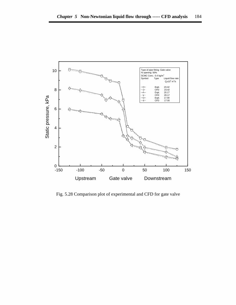
Chapter 5 Non-Newtonian liquid flow through ----- CFD analysis 184
-150 -100 -50 0 50 100 1500
2
4
6
8
10
Stat
ic p
ress
ure,
kPa
Upstream Gate valve Downstream
Type of pipe fitting: Gate valve% opening: 50%SCMC Conc.: 0.4 kg/m3
Symbol Type Liquid flow rate Q
lx105 m3/s
Expt. 23.42 CFD 23.42 Expt. 20.17 CFD 20.17 Expt. 17.00 CFD 17.00
Fig. 5.28 Comparison plot of experimental and CFD for gate valve

Chapter 5 Non-Newtonian liquid flow through ----- CFD analysis 185
0.6 0.8 1.0 1.2 1.4 1.6 1.8 2.0 2.2 2.40
1
2
3
4
5
6
7
8
9
Pres
uure
dro
p, k
Pa
Liquid velocity, m/s
Symbol Type Gate SCMC valve conc. opening kg/m3
(%) Expt. 50 0.8 CFD 50 0.8 Expt. 75 0.8 CFD 75 0.8 Expt. 100 0.8 CFD 100 0.8
Fig. 5.29 Comparison of the experimental data and CFD modeling for gate valve
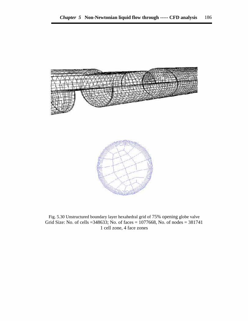
Chapter 5 Non-Newtonian liquid flow through ----- CFD analysis 186
Fig. 5.30 Unstructured boundary layer hexahedral grid of 75% opening globe valveGrid Size: No. of cells =348633; No. of faces = 1077668, No. of nodes = 381741
1 cell zone, 4 face zones
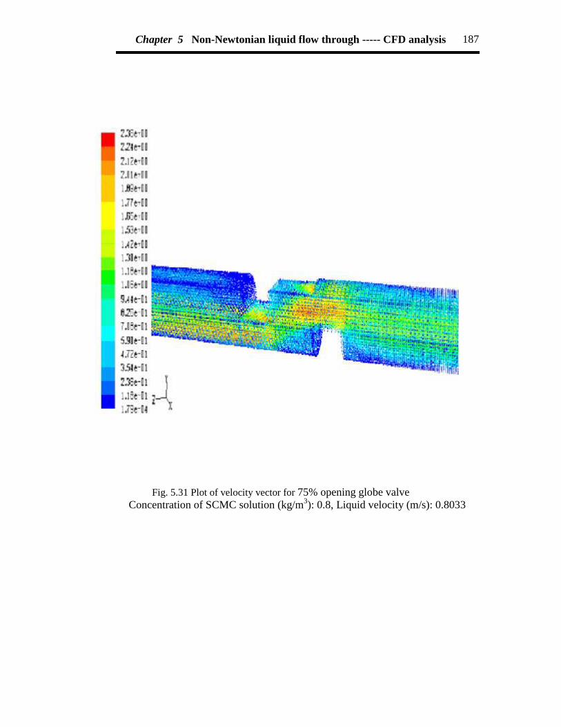
Chapter 5 Non-Newtonian liquid flow through ----- CFD analysis 187
Fig. 5.31 Plot of velocity vector for 75% opening globe valveConcentration of SCMC solution (kg/m3): 0.8, Liquid velocity (m/s): 0.8033

Chapter 5 Non-Newtonian liquid flow through ----- CFD analysis 188
-150 -100 -50 0 50 100 150
0
5
10
15
20
25St
atic
pre
ssur
e, k
Pa
Upstream Globe valve Downstream
Type of pipe fitting: Globe valve% opening: 75%SCMC Conc.: 0.2 kg/m3
Symbol Type Liquid flow rate Q
lx105
Expt. 22.67 CFD 22.67 Expt. 21.00 CFD 21.00
Fig. 5.32 Comparison plot of experimental and CFD for globe valve

Chapter 5 Non-Newtonian liquid flow through ----- CFD analysis 189
0.4 0.6 0.8 1.0 1.2 1.4 1.6 1.8
0
5
10
15
20
25
30
Pres
sure
dro
p, k
Pa
Liquid velocity, m/s
Symbol Type Globe SCMC valve conc. opening kg/m3
(%) Expt. 50 0.8 CFD 50 0.8 Expt. 75 0.8 CFD 75 0.8 Expt. 100 0.8 CFD 100 0.8
Fig. 5.33 Comparison of the experimental data and CFD modeling for globe valve
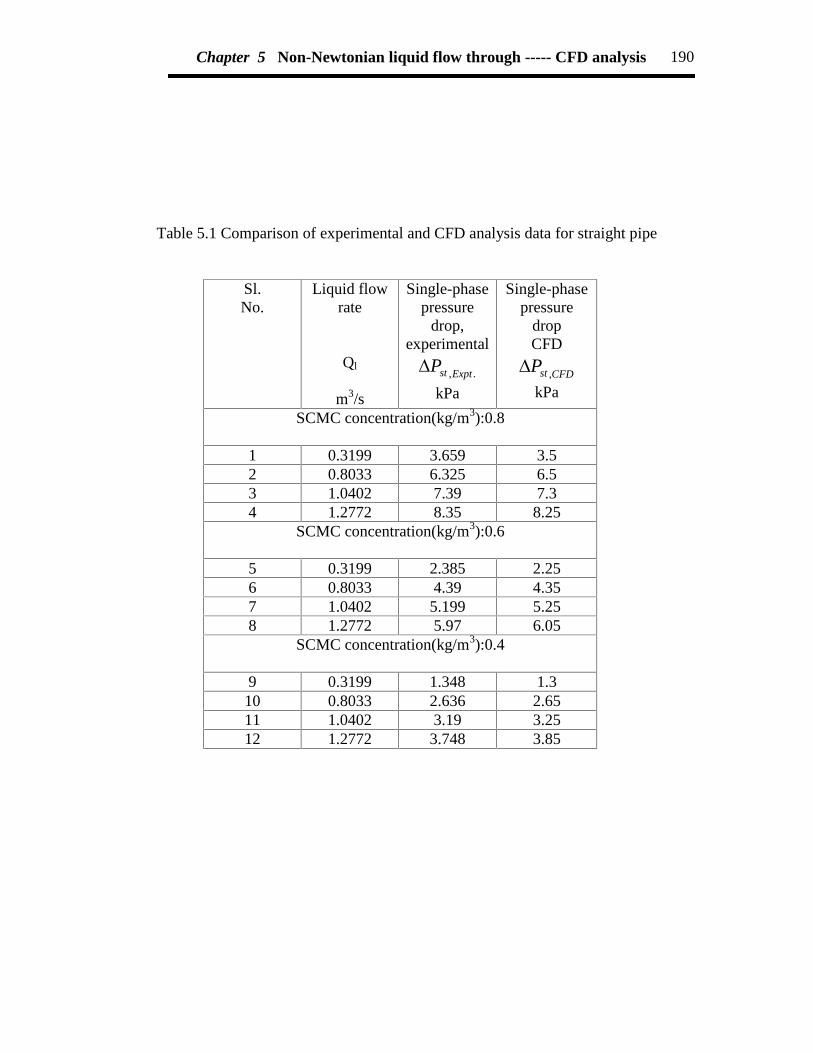
Chapter 5 Non-Newtonian liquid flow through ----- CFD analysis 190
Table 5.1 Comparison of experimental and CFD analysis data for straight pipe
Sl.No.
Liquid flowrate
Ql
m3/s
Single-phasepressure
drop,experimental
.,ExptstPkPa
Single-phasepressure
dropCFD
CFDstP ,kPa
SCMC concentration(kg/m3):0.8
1 0.3199 3.659 3.52 0.8033 6.325 6.53 1.0402 7.39 7.34 1.2772 8.35 8.25
SCMC concentration(kg/m3):0.6
5 0.3199 2.385 2.256 0.8033 4.39 4.357 1.0402 5.199 5.258 1.2772 5.97 6.05
SCMC concentration(kg/m3):0.4
9 0.3199 1.348 1.310 0.8033 2.636 2.6511 1.0402 3.19 3.2512 1.2772 3.748 3.85
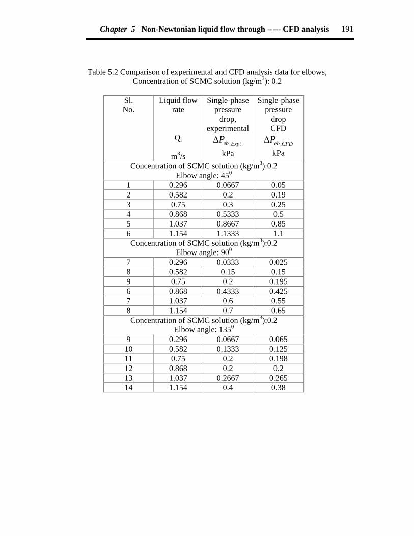
Chapter 5 Non-Newtonian liquid flow through ----- CFD analysis 191
Table 5.2 Comparison of experimental and CFD analysis data for elbows,Concentration of SCMC solution (kg/m3): 0.2
Sl.No.
Liquid flowrate
Ql
m3/s
Single-phasepressure
drop,experimental
.,ExptebPkPa
Single-phasepressure
dropCFD
CFDebP ,kPa
Concentration of SCMC solution (kg/m3):0.2Elbow angle: 450
1 0.296 0.0667 0.052 0.582 0.2 0.193 0.75 0.3 0.254 0.868 0.5333 0.55 1.037 0.8667 0.856 1.154 1.1333 1.1Concentration of SCMC solution (kg/m3):0.2
Elbow angle: 900
7 0.296 0.0333 0.0258 0.582 0.15 0.159 0.75 0.2 0.1956 0.868 0.4333 0.4257 1.037 0.6 0.558 1.154 0.7 0.65Concentration of SCMC solution (kg/m3):0.2
Elbow angle: 1350
9 0.296 0.0667 0.06510 0.582 0.1333 0.12511 0.75 0.2 0.19812 0.868 0.2 0.213 1.037 0.2667 0.26514 1.154 0.4 0.38

Chapter 5 Non-Newtonian liquid flow through ----- CFD analysis 192
Table 5.3 Comparison of experimental and CFD analysis data for orifice, Concentrationof SCMC solution (kg/m3): 0.8
Sl.No.
Liquid flowrate
Ql
m3/s
Single-phasepressure
drop,experimental
.,0 ExptPkPa
Single-phasepressure
dropCFD
CFDP ,0kPa
Concentration of SCMC solution (kg/m3):0.8Orifice diameter ratio, D0/ Dt : 0.4646
1 0.296 2 1.982 0.582 8.933 8.883 0.75 15.5 15.46674 0.868 23.75 23.73
Concentration SCMC solution (kg/m3):0.8Orifice diameter ratio, D0/ Dt: 0.5984
5 0.296 0.5 0.46 0.582 3.5 3.468 0.75 6.26 67 0.868 9.6 9.58Concentration of SCMC solution (kg/m3):0.2
Orifice diameter ratio, D0/ Dt: 0.70878 0.296 0.2666 0.259 0.582 1.25 1.2
10 0.75 2.266 2.211 0.868 3.866 3.65

Chapter 5 Non-Newtonian liquid flow through ----- CFD analysis 193
Table 5.4 Comparison of experimental and CFD analysis data for gate valve,Concentration of SCMC solution (kg/m3): 0.8
Sl.No.
Liquid flowrate
Ql
m3/s
Single-phasepressure
drop,experimental
.,ExptgatePkPa
Single-phasepressure
dropCFD
CFDgateP ,kPa
Concentration of SCMC solution (kg/m3):0.8Gate Valve, % opening: 50
1 0.8033 1.2 1.12 1.5142 4 4.123 2.2377 8.13 8
Concentration of SCMC solution (kg/m3):0.8Gate Valve, % opening: 75
5 0.8033 0.533 0.56 1.5142 2.133 27 2.2377 4.133 4Concentration of SCMC solution (kg/m3):0.8
Gate Valve, % opening: 1008 0.8033 0.5 0.59 1.5142 2 2
10 2.2377 3.93 4

Chapter 5 Non-Newtonian liquid flow through ----- CFD analysis 194
Table 5.5 Comparison of experimental and CFD analysis data for globe valve,Concentration of SCMC solution (kg/m3): 0.8
Sl.No.
Liquid flowrate
Ql
m3/s
Single-phasepressure
drop,experimental
.,ExptglobePkPa
Single-phasepressure
dropCFD
CFDglobeP,
kPa
Concentration of SCMC solution (kg/m3):0.8Globe Valve, % opening: 50
1 0.4407 1.733 1.52 0.8033 8.4 73 1.5142 23.6 234 1.639 25.73 24.75
Concentration of SCMC solution (kg/m3):0.8Globe Valve, % opening: 75
5 0.4407 1.5 1.456 0.8033 6 67 1.5142 17.46 178 1.639 22 21.5
Concentration of SCMC solution (kg/m3):0.8Globe Valve, % opening: 100
9 0.4407 1.25 1.1510 0.8033 5 4.511 1.5142 15 1412 1.639 18 17.5

Chapter 6
CFD analysis on two-phase gas-non-Newtonian liquid flowthrough piping components
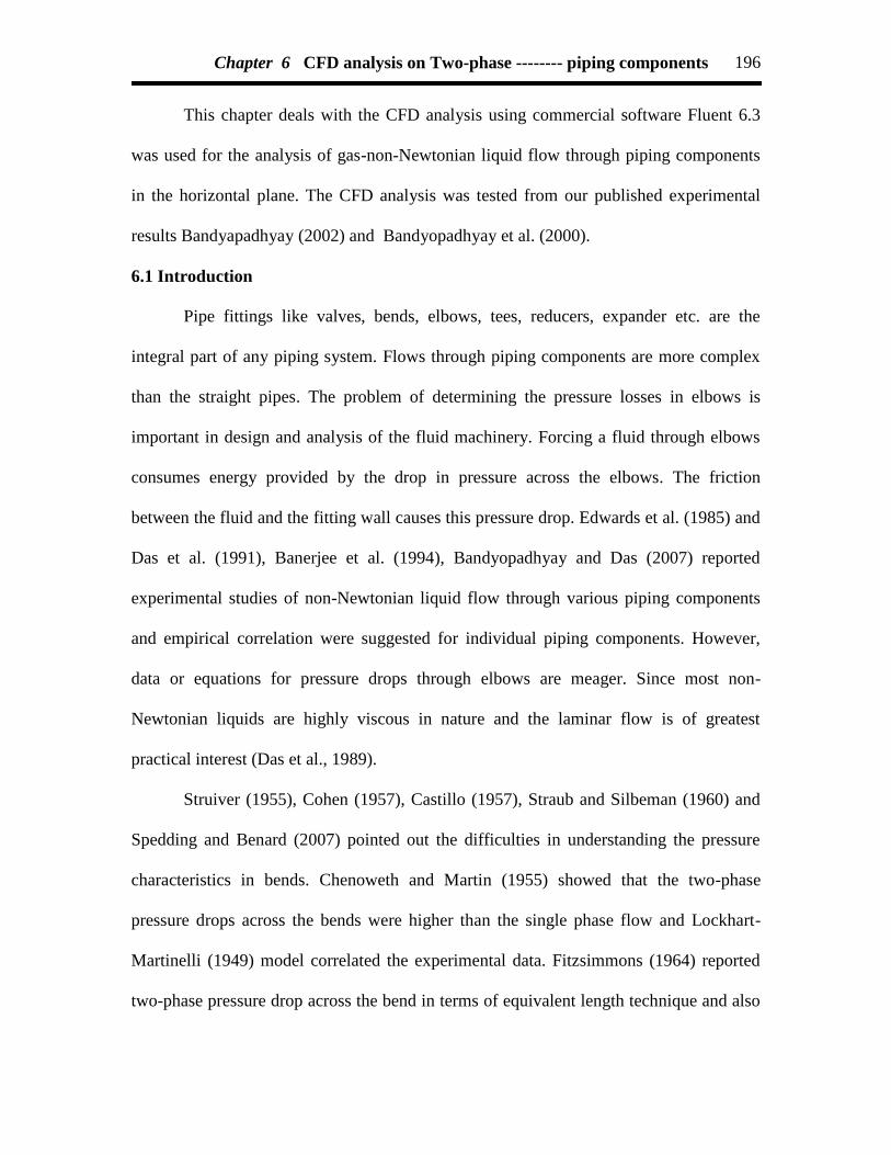
Chapter 6 CFD analysis on Two-phase -------- piping components 196
This chapter deals with the CFD analysis using commercial software Fluent 6.3
was used for the analysis of gas-non-Newtonian liquid flow through piping components
in the horizontal plane. The CFD analysis was tested from our published experimental
results Bandyapadhyay (2002) and Bandyopadhyay et al. (2000).
6.1 Introduction
Pipe fittings like valves, bends, elbows, tees, reducers, expander etc. are the
integral part of any piping system. Flows through piping components are more complex
than the straight pipes. The problem of determining the pressure losses in elbows is
important in design and analysis of the fluid machinery. Forcing a fluid through elbows
consumes energy provided by the drop in pressure across the elbows. The friction
between the fluid and the fitting wall causes this pressure drop. Edwards et al. (1985) and
Das et al. (1991), Banerjee et al. (1994), Bandyopadhyay and Das (2007) reported
experimental studies of non-Newtonian liquid flow through various piping components
and empirical correlation were suggested for individual piping components. However,
data or equations for pressure drops through elbows are meager. Since most non-
Newtonian liquids are highly viscous in nature and the laminar flow is of greatest
practical interest (Das et al., 1989).
Struiver (1955), Cohen (1957), Castillo (1957), Straub and Silbeman (1960) and
Spedding and Benard (2007) pointed out the difficulties in understanding the pressure
characteristics in bends. Chenoweth and Martin (1955) showed that the two-phase
pressure drops across the bends were higher than the single phase flow and Lockhart-
Martinelli (1949) model correlated the experimental data. Fitzsimmons (1964) reported
two-phase pressure drop across the bend in terms of equivalent length technique and also

Chapter 6 CFD analysis on Two-phase -------- piping components 197
Lockhart-Martinelli (1949) correlation and observed that the experimental data were very
poorly correlated using these techniques. Sekoda et al. (1969) reported the flow
characteristics in the inlet and outlet region of 900 bend. They also observed that the two-
phase pressure drop was independent of the pipe diameter but depends on the ratio of
Dc/d. Bruce (1971) observed that the two-phase pressure drop across the bends was over
predicted by using the conventional Lockhart-Martinelli (1949) correlation for the vapour
liquid R12 refrigerant flow through bends. Engineering Science Data Unit (1977) reported
model for two-phase flow through piping components. Maddock et al. (1974) reported
the structure of two-phase flow in curved geometry. Hoang and Davies (1984) showed
that flow regime changes from bubbly inlet flow to stratified flow at the outlet of the 180o
bend. Deobold (1962) claimed that the horizontal bend, horizontal to vertical up bend and
the vertical down to horizontal bend all gave the same bend pressure loss. However, a
horizontal to vertical down bend had a pressure drop was 35% less. Xin et al. (1996)
reported the numerical modeling of turbulent single-phase and two-phase flow in curved
pipe and observed discrepancies between the prediction and observed values in two-
phase flow. Azzi et al. (2000) and Azzi et al. (2002) pointed out that no model describes
the properties of the two-phase gas-liquid flow through bends. Supa-Amornkul et al.
(2005) reported the CFD modeling of two-phase air water flow through pipe bends. They
observed that the simulation for two-phase flow was significantly different from the
experimental data. i.e., the overall pressure drop across the test section was significantly
less for the simulation than for the experimental data. Spedding et al. (2007) correlated
the two-phase pressure drop across the elbow in terms of total Reynolds number.

Chapter 6 CFD analysis on Two-phase -------- piping components 198
The availability of the literature for gas-non-Newtonian liquid flow through
piping components is very sporadic (Das et al., 1991). Das et al. (1991), Banerjee and
Das (1998), Samanta et al. (1999) and Bandyopadhyay et al. (2000) reported the
experimental investigation for gas-non-Newtonian liquid flow through bends, valves,
orifices and elbows. They developed empirical correlation for predicting the frictional
pressure drop across the piping components. In order to achieve optimum performance,
an accurate design technique is necessary for the prediction of the pressure drop for gas-
non-Newtonian liquid through piping components.
The use of CFD in designing engineering devices has increased over the last few
years due to availability of commercial codes featuring state-of-the-art robust models and
the ability to run the code on desktop PCs. Evaluating two-phase pressure losses across
the piping components using continuum and particulate phase in the Eulerian/Lagrangian
approach or as a homogeneous fluid in the Eulerian/Eulerian approach. The objective of
this chapter is to validate the CFD model of the commercial code Fluent 6.3 for
predicting the two-phase gas-non-Newtonian pressure drop across the straight pipe and
the piping components and tested the model with our previous experimental data from
our laboratory by Bandyopadhyay (2002) and Bandyopadhyay et al. (2000).
6.2 The experimental setup
Details of the experimental (Fig. 6.1) investigation for gas-non-Newtonian liquid
flow through piping components are reported in our earlier work published by
Bandyopadhyay (2002) and Bandyopadhyay et al. (2000). The ranges of variables
investigated are shown in Tables 6.1.
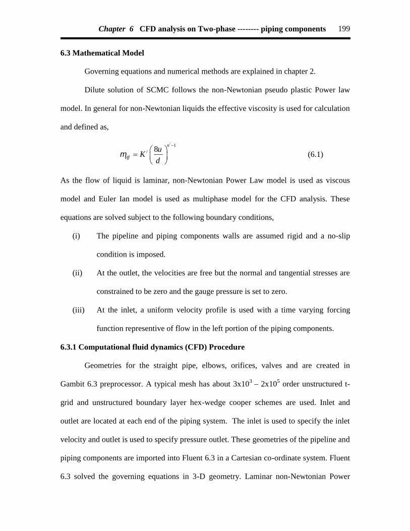
Chapter 6 CFD analysis on Two-phase -------- piping components 199
6.3 Mathematical Model
Governing equations and numerical methods are explained in chapter 2.
Dilute solution of SCMC follows the non-Newtonian pseudo plastic Power law
model. In general for non-Newtonian liquids the effective viscosity is used for calculation
and defined as,
/ 1/ 8
n
eff
uK
d
(6.1)
As the flow of liquid is laminar, non-Newtonian Power Law model is used as viscous
model and Euler Ian model is used as multiphase model for the CFD analysis. These
equations are solved subject to the following boundary conditions,
(i) The pipeline and piping components walls are assumed rigid and a no-slip
condition is imposed.
(ii) At the outlet, the velocities are free but the normal and tangential stresses are
constrained to be zero and the gauge pressure is set to zero.
(iii) At the inlet, a uniform velocity profile is used with a time varying forcing
function representive of flow in the left portion of the piping components.
6.3.1 Computational fluid dynamics (CFD) Procedure
Geometries for the straight pipe, elbows, orifices, valves and are created in
Gambit 6.3 preprocessor. A typical mesh has about 3x10³ – 2x10⁵ order unstructured t-
grid and unstructured boundary layer hex-wedge cooper schemes are used. Inlet and
outlet are located at each end of the piping system. The inlet is used to specify the inlet
velocity and outlet is used to specify pressure outlet. These geometries of the pipeline and
piping components are imported into Fluent 6.3 in a Cartesian co-ordinate system. Fluent
6.3 solved the governing equations in 3-D geometry. Laminar non-Newtonian Power

Chapter 6 CFD analysis on Two-phase -------- piping components 200
Law model have been used for simulation. The model solves for Navier-stokes equation
at prescribes velocities. The governing equations are non linear and several iterations of
loop must be performed before a convergent solution is obtained. The first-order upwind
scheme is used in the discretization of set of governing equations, standard interpolation
schemes is used for calculating cell-face pressures for using the Segregated solver in
Fluent 6.3. Pressure-velocity coupling refers to the numerical algorithm which uses a
combination of continuity and momentum equations to derive an equation for pressure
(or pressure correction) when using the segregated solver. Simple algorithm is used.
A general procedure to simulate the two-phase gas-non-Newtonian fluid flow
through pipe and piping components based on Gambit 6.3 and Fluent 6.3 software is
outlined below,
1. Perform meshing under Gambit 6.3.
Create a computational domain at the flow region,
The grids were generated using boundary layer hexahedral meshes and t-
grid (tetrahedral grid),
Controlling a smooth change in the mesh size by size functions,
Specify boundary and continuum types,
Examine the mesh to ensure that the high skewness is below 0.5 for
hexahedral and below 0.9 for tetrahedral mesh.
2. Import the mesh file to Fluent 6.3 and check the mesh.
3. Define a 3-D, unsteady, implicit, and pressure-based solver.
4. Activate the Eulerian laminar non-Newtonian power law multiphase model.
5. Define Eulerian laminar model. Slip velocity is added.
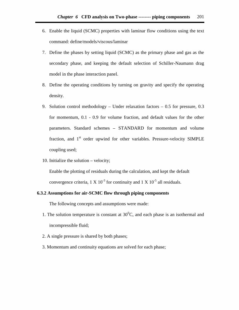
Chapter 6 CFD analysis on Two-phase -------- piping components 201
6. Enable the liquid (SCMC) properties with laminar flow conditions using the text
command: define/models/viscous/laminar
7. Define the phases by setting liquid (SCMC) as the primary phase and gas as the
secondary phase, and keeping the default selection of Schiller-Naumann drag
model in the phase interaction panel.
8. Define the operating conditions by turning on gravity and specify the operating
density.
9. Solution control methodology – Under relaxation factors – 0.5 for pressure, 0.3
for momentum, 0.1 - 0.9 for volume fraction, and default values for the other
parameters. Standard schemes – STANDARD for momentum and volume
fraction, and 1st order upwind for other variables. Pressure-velocity SIMPLE
coupling used;
10. Initialize the solution – velocity;
Enable the plotting of residuals during the calculation, and kept the default
convergence criteria, 1 X 10⁻³ for continuity and 1 X 10⁻⁵ all residuals.
6.3.2 Assumptions for air-SCMC flow through piping components
The following concepts and assumptions were made:
1. The solution temperature is constant at 300C, and each phase is an isothermal and
incompressible fluid;
2. A single pressure is shared by both phases;
3. Momentum and continuity equations are solved for each phase;

Chapter 6 CFD analysis on Two-phase -------- piping components 202
4. Our system behaves like a plug and slug flow regimes. But we assumed two-phase
flow as a bubbly flow due to simplicity of calculation in which liquid (SCMC) is
treated as the primary phase while gas is treated as the secondary phase;
5. The secondary phase consists of uniform and unchanging bubbles dispersed in a
continuous phase;
6. The bubbles size is assumed to be small, 0.1mm spherical in size;
7. Two–phase Eulerian laminar non-Newtonian power law model is used;
8. Physical properties are uniform throughout;
9. Different phases move at different velocities (slip velocities);
10. The drag force from liquid (SCMC) phase acting on the gas bubbles is included
into the interphase momentum exchange;
11. There are no external body force and virtual mass force, and the effect of lift force
on the bubbles is negligible.
6.4 Results and discussion
6.4.1 Convergence and grid independency
The convergence criterions were set at 10-5 for all equations except for the
transport equation which residual was set at 10-3. A computational domain L≥200D was
used to ensure fully developed flow results could be obtained for all pipe and piping
components. In general the final results depend upon mesh geometries. Subsequent
decrement and increment in mesh resolution by 50% were applied to evaluate if the
employed mesh resolution was adequate to obtain accurate solutions. It was observed that
when the mesh resolution was decreased by 50% the axial velocity profile was 7-12% of
the currently employed mesh velocity profile for pipe and different piping components.

Chapter 6 CFD analysis on Two-phase -------- piping components 203
As the present mesh resolution was increased by 50% the axial velocity profile changes
1-3% for pipe and different piping components. These results suggest that the current
mesh resolution is sufficient to obtained grid independent solutions for the proposed
model.
6.4.2 Computational fluid dynamics (CFD) analysis for air-non-Newtonian liquidflow through straight pipe
Fig. 6.2 shows the contour plot of velocity vector in the air-SCMC mixture for
straight pipe. It illustrates that velocity is maximum at centre and velocity is minimum
near the wall of the pipe. Figs. 6.3 and 6.4 show the velocity vector plot of liquid phase
and air phase in the mixture for straight pipe. It indicates that heavier density liquid phase
more at the nearer to the wall and lighter air phase more at the centre of the pipe. Fig. 6.5
shows that contours of velocity magnitude at the different points of straight pipe. It
illustrates that velocity is maximum at centre and velocity is minimum near the wall of
the pipe. Fig. 6.6 shows that contours of axial velocity at the different points of straight
pipe. It indicates that some air pockets observed with the liquid.
Figs. 6.7 and 6.8 show the Contour plot of static pressure and total pressure
(mixture) at the different points of the straight pipe. It indicates that static pressure and
total pressure gradually decreases from inlet to outlet of the pipe due to fluid-pipe
friction. This effect is more with increasing the liquid concentration. Figs. 6.9 and 6.10
show that the contours plot of volume fraction at liquid and air phase. It indicates that air
concentration is more at the centre and liquid concentration is more neighboring position
of the centre and nearer to the wall.
Fig. 6.11 indicates that two-phase frictional pressure drop increases with
increasing liquid flow rate.

Chapter 6 CFD analysis on Two-phase -------- piping components 204
Fig. 6.12 indicates that two-phase frictional pressure drop increases with
increasing SCMC concentration in the liquid, i.e., pseudoplacticity of the liquid.
Fig.13 shows that comparison of experimental results with CFD simulated results
for different liquid flow rate. In both cases experimental results matches well with the
CFD simulated results. From this plot we see that both result matches with error% ±10.
6.4.3 Computational fluid dynamics (CFD) analysis for air-non-Newtonian liquidflow through elbows
Fig.6.14 illustrates the contour plot of velocity for the gas-liquid mixture for 450
elbows. Fig. 6.15 (a-c) shows that contour plot of velocity at different points in the
elbows. It is clear from these figures the mixture velocity is higher at the centre position
and inner side of the elbow and lowers at the outer wall. As the mixture enters to the
elbows due to centrifugal action heavier density phase that is liquid moves to the outer
wall and lower density phase, air moves to the inner wall. Fig. 6.16 clearly demonstrates
that the liquid velocity is higher at the outer wall. Fig. 6.17 illustrates that the air velocity
at the inner wall is higher and practically zero at the outer wall. The inlet flow regime is
intermittent in nature (plug and slug). At inlet the existence of air is at the top. Due to slip
exist between the liquid and air and the existence of the pressure gradient across the
cross-section air velocity increases compare to the liquid velocity, due to centrifugal
action the liquid is shifted towards the outer wall and a stratified flow condition attaint
within the elbows.
Fig. 6.18 shows the static pressure profile of elbows. The 45o elbow shows higher
pressure drop than comparing with the other elbows and it is due to faster dispersion of
rope and a shorter developing flow exist. Fig. 6.19 shows that contour plot of static
pressure at different points in the elbows. It shows that pressure is high at outer wall as

Chapter 6 CFD analysis on Two-phase -------- piping components 205
heavier density liquid phase goes to outer wall due to centrifugal force and low at the
inner wall when the air phase exists. Due to this pressure gradient at any cross section of
the elbow the air is accelerated more than the liquid phase. Due to this acceleration
maximum velocity is shifted for the mixer.
The secondary flow originated in a pair of counter rotating vortices at the just
inside of the elbow as shown in Fig. 6.20 for 450 elbows. These vortices continue up to
the downstream of the elbow, merged in the just outlet of the elbow and downstream flow
return slowly to the steady state.
Fig. 6.21 shows that volume fraction of the liquid (SCMC) and air at different
point in the 900 elbow. It shows that heavier density phase liquid (SCMC) goes to outer
wall side and lighter air goes to inner wall side due to centrifugal force.
Fig. 6.22 shows that comparison plot of static pressure experimental and CFD for
450 elbows. Fig. 6.23 shows that comparison plot of experimental results with CFD
simulated results at different elbow angles. In both cases experimental results matches
well with the CFD simulated results.
The flow pattern is depended on the flow rate of each phase, their interactions the
transport properties and the geometry of the elbows. The flow regime was difficult to
determine in the two-phase region. In general an accumulation of air towards the inside
of the wall, this originates from the start of the elbow. This could be caused by a radial
pressure gradient generated by the lower density mixture causing the slow-moving liquid
phase near the wall to move toward the inside wall of the elbow. Phenomenon at high gas
flow rates was observed by Banerjee et al. (1967), Farukhi and Parker (1974), Maddock
et al. (1974) and Usui et al. (1983).

Chapter 6 CFD analysis on Two-phase -------- piping components 206
6.4.4 Computational fluid dynamics (CFD) analysis for air-non-Newtonian liquidflow through orifices
Figs. 6.24 - 6.26 show that contour plot of velocity vector in the air-SCMC
mixture at the different cross-section of orifices. It indicates that velocity is low at the
inlet of the pipe and it increases more after passing the orifice plate. This is due to
narrowing of the flow area. It affects more from large orifice diameter to small orifice
diameter.
Figs. 6.27 - 6.29 show that contour plot of static pressure (mixture) for three
orifices. It indicates that static pressure is high from inlet of the pipe to up to inlet of
orifice and it decreases more after passing the orifice plate. This is due to narrowing of
the flow area. It affects more from large orifice diameter to small orifice diameter. Figs.
6.30 – 6.32 show that velocity vector plot for mixture, liquid and air phase. Figs. 6.33 –
6.34 show that velocity magnitude and velocity at the different points of orifices. Figs.
6.35 – 6.36 show that static pressure and total pressure plot in the mixture at different
points of orifice. Fig. 6.37 shows the contour of volume fraction for liquid phase at
different cross section of the orifice. It indicates that liquid percentage is maximum at the
centre of the orifice plate. It also indicates that after passing the orifice plate liquid
percentage slightly decrease at the centre in compare to orifice plate but its surrounding
place liquid percentage is very low. Fig. 6.38 shows the contour of volume fraction for air
phase at different cross section of the orifice. It indicates that air percentage is minimum
at the centre of the orifice plate. It also indicates that after passing through the orifice
plate liquid percentage is slightly increase at the centre in compare to orifice plate due the
presence of vena contracta.

Chapter 6 CFD analysis on Two-phase -------- piping components 207
Fig. 6.39 comparison of the experimental result with CFD simulated result with
different liquid flow rate and fixed liquid concentration, fixed orifice dimension. It
indicates that two-phase frictional pressure drop increases with increasing liquid flow
rate. This is due to with increasing the flow rate, increasing the velocity and more
increasing the velocity more increasing of kinetic energy causing loss as a form of
pressure energy.
Fig. 6.40 shows that comparison of the experimental result with CFD simulated
result with different orifice dimension and fixed liquid concentration, fixed liquid flow
rate. It indicates that two-phase frictional pressure drop increases with decreasing orifice
diameter. This is due to decreasing of flow area velocity increases and according to
Bernoulli’s conservation law pressure drop increase.
Fig. 6.41 shows that comparison plot of experimental results with CFD simulated
results for different liquid flow rates. Fig. 6.42 shows that comparison of experimental
results with CFD simulated results for different Orifice diameter ratios.
In both cases experimental results matches well with the CFD simulated results.
6.4.5 Computational fluid dynamics (CFD) analysis for air-non-Newtonian liquidflow through gate valve
Fig. 6.43 shows that plot of velocity vector in the air-non-Newtonian liquid
mixture at different points of the 50% opening gate valve. It indicates that velocity
increases at the position of the 50% opening gate valve. This is due to lowering of flow
area. Similar velocity vector plot observed for 75% and 100% opening gate valve. It is
noted that velocity increases from 100% opening valve to 50% opening valve. This is due
to lowering of flow area which causing increasing of velocity. Figs. 6.44 - 6.45 show that
contours of velocity magnitude and velocity in the air-non-Newtonian mixture at

Chapter 6 CFD analysis on Two-phase -------- piping components 208
different points of the 50% opening gate valve. It indicates that velocity increases at the
valve position. This is due to narrowing the flow area. It is also observed that some
secondary flow is observed.
Figs. 6.46 and 6.47 show that contour plot of static pressure and total pressure for
50% opening gate valve. It indicates that static pressure decreases after passing the valve.
It affects more with increasing the obstruction i.e. decreasing the flow area, decreasing
the valve and increasing the pseudoplasticity of the liquid. This is due to obstruction of
flow causing increase of kinetic energy as a form of lowering of pressure. Similar plot
observed for 75% and 100% opening gate valve. It is noted that static pressure decreases
too much from 100% opening valve to 50% opening valve. This is due to lowering of
flow area which causing decreasing of static pressure by increasing the velocity
according to Bernoulli’s conservation law. Fig. 6.48 and Fig. 6.49 show that contours of
volume fraction for liquid phase and air-phase at the different points of the 50% opening
gate valve. It indicates that at the valve position lighter density gas passing slightly lower
than heavier density liquid phase.
Fig. 6.50 shows that comparison of experimental results with CFD simulated
results for different liquid flow rates. It indicates that two-phase frictional pressure drop
increases with increasing liquid flow rate. This is due to with increasing the flow rate,
increasing the velocity and more increasing the velocity more increasing of kinetic
energy causing loss as a form of pressure energy. Fig.6.51 shows that comparison of
experimental results with CFD simulated results for different % opening of Gate valve. It
indicates that two-phase frictional pressure drop increases with decreasing valve opening.
This is due to decreasing of flow area velocity increases and according to Bernoulli’s

Chapter 6 CFD analysis on Two-phase -------- piping components 209
conservation law pressure drop increases. In both cases Experimental results matches
well with the CFD simulated results.
6.4.6 Computational fluid dynamics (CFD) analysis for air-non-Newtonian liquidflow through globe valve
Figs. 6.52 - 6.53 show that plot of velocity vector in the air-SCMC mixture at the
different points of 50% opening globe valve. It indicates that velocity increases due to
decreasing of flow area. Figs. 6.54 - 6.55 show that plot of velocity vector for liquid
phase and air phase in the air-non-Newtonian mixture at the different points of 50%
opening globe valve. It indicates that heavier density liquid phase goes to the wall side
more at the valve position. Whereas lighter density air-phase more at the central position
of valve. Figs. 6.56 - 6.57 show that Contour plot of velocity magnitude and axial
velocity. It illustrates that velocity is more at the valve position due to lowering of flow
area and also observed the secondary flow, vortices generated at the some position.
Figs. 6.58 - 6.59 show that Contour plot of static pressure and total pressure for
50%, opening globe valve. Similar plot is observed for 75%, 100% opening globe valve.
It indicates that static pressure decreases more after passing the valve. This is due to
increasing velocity, increasing of kinetic energy as a form of lowering of static pressure
according to Bernoulli’s conservation law. Both pressure decreases from 100%, 75%,
50% due to increasing of obstruction.
Figs. 6.60 - 6.61 show that contour plot of volume fraction for liquid phase and air
phase in the air-non-Newtonian liquid mixture at the different points of 50% opening
globe valve. It indicates that heavier density liquid phase goes to the wall side more at the
valve position. Whereas lighter density air-phase more at the central position of valve.

Chapter 6 CFD analysis on Two-phase -------- piping components 210
Fig. 6.62 shows that comparison of the experimental result with CFD simulated
result with different liquid flow rate and fixed liquid concentration, fixed valve
dimension. It indicates that two-phase frictional pressure drop increases with increasing
liquid flow rate. This is due to with increasing the flow rate, increasing the velocity and
more increasing the velocity more increasing of kinetic energy causing loss as a form of
pressure energy.
Fig. 6.63 shows that comparison plot of experimental results with CFD simulated
results for different liquid flow rates. Fig. 6.64 shows that comparison plot of
experimental results with CFD simulated results for different % opening of Globe valve.
It indicates that two-phase frictional pressure drop increases with decreasing valve
opening. This is due to decreasing of flow area velocity increases and according to
Bernoulli’s conservation law pressure drop increases.
In both cases Experimental results matches well with the CFD simulated results.
6.5 Conclusions
1. Computational Fluid Dynamics (CFD) analysis has been reported for gas-non-
Newtonian liquids flow through straight pipe and piping components in the horizontal
plane.
2. In case of gas-non-Newtonian liquid flow through horizontal pipe the CFD analysis
predicts,
i. The velocity and pressure field at different points in the elbows for air-liquid
mixture and individual phases.
ii The contour plots of velocity magnitude at the different points of straight pipe
illustrates that velocity is maximum at centre and velocity is minimum near the

Chapter 6 CFD analysis on Two-phase -------- piping components 211
wall of the pipe. The contour plots of the axial velocity at the different points of
straight pipe indicate that some air pockets observed with the liquid.
iii. Contour plots of static pressure and total pressure (mixture) at the different points
of the straight pipe indicates that static pressure and total pressure gradually
decreases from inlet to outlet of the pipe due to fluid-pipe friction. This effect is
more with increasing the liquid concentration.
iv. Contour plots of volume fraction at liquid and air phase indicates that air
concentration is more at the centre and liquid concentration is more neighboring
position of the centre and nearer to the wall.
3. In case of gas-non-Newtonian liquid flow through elbows the CFD analysis predicts,
i. The velocity and pressure field at different points in the elbows for air-SCMC
mixture and individual phases.
ii. As the mixture enters to the elbows due to centrifugal action heavier density
phase that is liquid moves to the outer wall and lower density phase, air moves to
the inner wall. The static pressure profile of elbows show that for 45o elbow
pressure drop is more comparing to the 135o elbow. Static pressure is high at
outer wall as heavier density liquid phase goes to outer wall due to centrifugal
force and low at the inner wall when the air phase exits.
iii. Contour plots of volume fraction show that heavier density liquid (SCMC) phase
goes to outer wall side and lighter air goes to inner wall side.
4. In case of gas-non-Newtonian liquid flow through orifices the CFD analysis predicts
i. velocity and pressure field at different points in the orifices for air-SCMC mixture
and individual phases,

Chapter 6 CFD analysis on Two-phase -------- piping components 212
ii. velocity is low at the inlet of the pipe and it increases more after passing the
orifice plate. This is due to narrowing of the flow area. It affects more from large
orifice diameter to small orifice diameter.
iii. Static pressure is high from inlet of the pipe to up to inlet of orifice and it
decreases more after passing the orifice plate. This is due to narrowing of the flow
area. It affects more from large orifice diameter to small orifice diameter.
iv. Contour plots of volume fraction for liquid phase at different cross section of the
orifice indicates that liquid percentage is maximum at the centre of the orifice
plate. It also indicates that after passing the orifice plate liquid percentage slightly
decrease at the centre in compare to orifice plate but its surrounding place liquid
percentage is very low. contour of volume fraction for air phase at different cross
section of the orifice indicates that air percentage is minimum at the centre of the
orifice plate. It also indicates that after passing through the orifice plate liquid
percentage is slightly increase at the centre in compare to orifice plate due the
presence of vena contracta.
5. In case of gas-non-Newtonian liquid flow through gate and globe valves the CFD
analysis predicts,
i. The velocity and pressure field at different points in the gate and globe valves for
air-liquid mixture and individual phases.
ii. The velocity increases at the valve position. This is due to narrowing the flow
area. It is also observed that some secondary flow is observed. Velocity is more
for 50% opening gate and globe valve. Static pressure decreases after passing the
valve. It affects more with increasing the obstruction, i.e., decreasing the flow

Chapter 6 CFD analysis on Two-phase -------- piping components 213
area, decreasing the valve and increasing the pseudoplasticity of the liquid. This is
due to obstruction of flow causing increase of kinetic energy as a form of
lowering of pressure. Static pressure decreases too much from 100% opening
valve to 50% opening valve. This is due to lowering of flow area which causing
decreasing of static pressure by increasing the velocity according to Bernoulli’s
conservation law.
iv. The volume fraction for liquid phase and air-phase at the different points of the
50% opening gate and globe valve indicates that at the valve position lighter
density gas passing slightly lower than heavier density liquid phase.

Chapter 6 CFD analysis on Two-phase -------- piping components 214
A: Compressor, B: Oil Tray, C: Gas Cylinder, D: Gas Regulator, E: Storage tank, P:Pump, P1 – P10: Manometer, RL1 – RL2: Liquid Rota meter, RG1 – RG2: Gas Rota meter,ST: Stirrer, T: T – Mixer, T1 – T2: Thermometer, V1 – V10: Valves, SV1: Solenoid valve
Fig. 6.1 Schematic diagram of the experimental setup
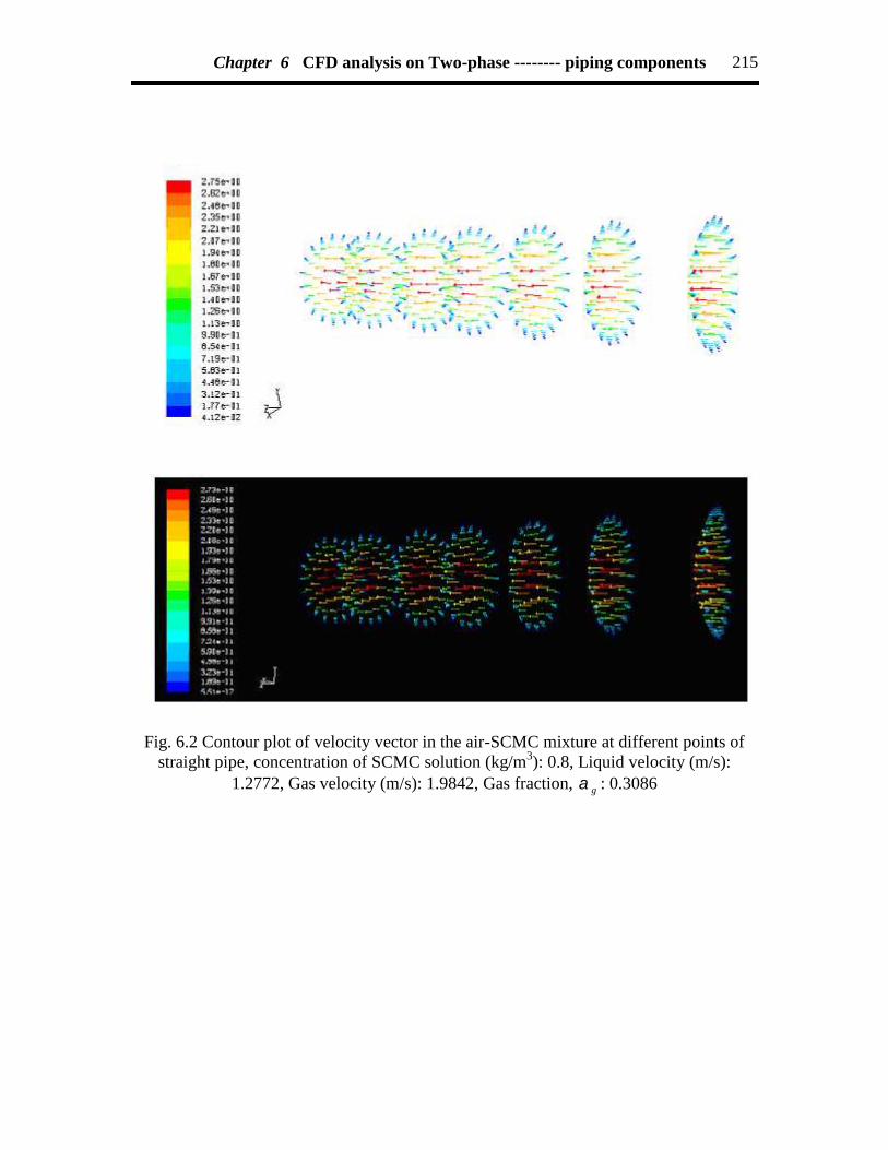
Chapter 6 CFD analysis on Two-phase -------- piping components 215
Fig. 6.2 Contour plot of velocity vector in the air-SCMC mixture at different points ofstraight pipe, concentration of SCMC solution (kg/m3): 0.8, Liquid velocity (m/s):
1.2772, Gas velocity (m/s): 1.9842, Gas fraction, g : 0.3086

Chapter 6 CFD analysis on Two-phase -------- piping components 216
Fig. 6.3 Contour plot of velocity vector for SCMC phase in the mixture at different pointsof straight pipe, SCMC concentration (kg/m3): 0.8, Liquid velocity (m/s): 1.2772, Gas
velocity (m/s): 1.9842, Gas fraction, g : 0.3086

Chapter 6 CFD analysis on Two-phase -------- piping components 217
Fig. 6.4 Plot of velocity vector for air phase in the mixture at different points of straightpipe, concentration of SCMC solution (kg/m3): 0.8, Liquid velocity (m/s): 1.2772, Gas
velocity (m/s): 1.9842, Gas fraction, g : 0.3086
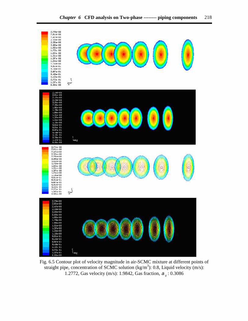
Chapter 6 CFD analysis on Two-phase -------- piping components 218
Fig. 6.5 Contour plot of velocity magnitude in air-SCMC mixture at different points ofstraight pipe, concentration of SCMC solution (kg/m3): 0.8, Liquid velocity (m/s):
1.2772, Gas velocity (m/s): 1.9842, Gas fraction, g : 0.3086

Chapter 6 CFD analysis on Two-phase -------- piping components 219
Fig. 6.6 Contour plot of axial velocity inside the different points of straight pipe,Concentration of SCMC solution (kg/m3): 0.8, Liquid velocity (m/s): 1.2772,
Gas velocity (m/s): 1.9842, Gas fraction, g : 0.3086

Chapter 6 CFD analysis on Two-phase -------- piping components 220
Fig. 6.7 Contours of static pressure inside the different points of straight pipe,Concentration of SCMC solution (kg/m3): 0.8, Liquid velocity (m/s): 1.2772,
Gas velocity (m/s): 1.9842, Gas fraction, g : 0.3086

Chapter 6 CFD analysis on Two-phase -------- piping components 221
Fig. 6.8 Contours of total pressure inside the different points of straight pipe,Concentration of SCMC solution (kg/m3): 0.8, Liquid velocity (m/s): 1.2772,
Gas velocity (m/s): 1.9842, Gas fraction, g : 0.3086

Chapter 6 CFD analysis on Two-phase -------- piping components 222
Fig. 6.9 Contours of SCMC phase volume fraction at different points of straight pipe,concentration of SCMC solution (kg/m3): 0.8, Liquid velocity (m/s): 1.2772, Gas velocity
(m/s): 1.9842, Gas fraction, g : 0.3086

Chapter 6 CFD analysis on Two-phase -------- piping components 223
Fig. 6.10 Contours of air phase volume fraction at different points of straight pipe,concentration of SCMC solution (kg/m3): 0.8, Liquid velocity (m/s): 1.2772, Gas velocity
(m/s): 1.9842, Gas fraction, g : 0.3086

Chapter 6 CFD analysis on Two-phase -------- piping components 224
2 4 6 8 10 12 14 16 18 20 22 242
4
6
8
10
12
14
16
18
20
Two
- pha
se p
ress
ure
drop
, kpa
Gas flow rate, Qg x 105 kg/m3
SCMC Conc.: 0.2 kg/m3
Type of piping component: Straight pipe
Symbol Type Liquid flow rate Q
l x 10-5, m3/s
Expt. 4.05 CFD 4.05 Expt. 7.00 CFD 7.00 Expt. 9.80 CFD 9.80 Expt. 13.17 CFD 13.17
Fig. 6.11 Comparison of the experimental data and CFD modeling for straight pipevarying with liquid flow rate

Chapter 6 CFD analysis on Two-phase -------- piping components 225
4 6 8 10 12 14 16 18 20 22 244
6
8
10
12
14
16
18
Two
- pha
se p
resu
re d
rop,
kpa
Gas flow rate, Qg x 105
Type of piping component: Straight pipeLiquid flow rate: 7.00 x 10⁻⁵
Symbol Type SCMC Conc. kg/m3
Expt. 0.2 CFD 0.2 Expt. 0.4 CFD 0.4 Expt. 0.6 CFD 0.6 Expt. 0.8 CFD 0.8
Fig. 6.12 Comparison of the experimental data and CFD modeling for straight pipevarying with SCMC solution concentration
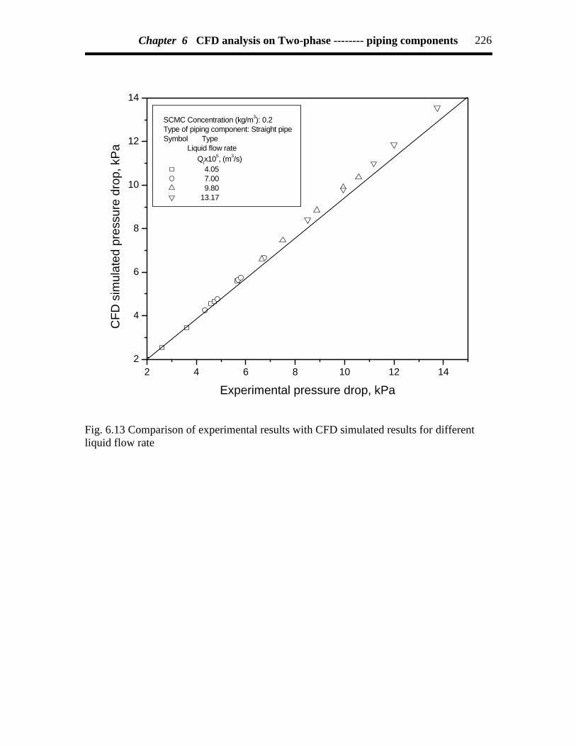
Chapter 6 CFD analysis on Two-phase -------- piping components 226
2 4 6 8 10 12 142
4
6
8
10
12
14
CFD
sim
ulat
ed p
ress
ure
drop
, kPa
Experimental pressure drop, kPa
SCMC Concentration (kg/m3): 0.2Type of piping component: Straight pipeSymbol Type Liquid flow rate Qlx105, (m3/s)
4.05 7.00 9.80 13.17
Fig. 6.13 Comparison of experimental results with CFD simulated results for differentliquid flow rate

Chapter 6 CFD analysis on Two-phase -------- piping components 227
Fig. 6.14 Contour plot of velocity vector for air-SCMC mixture at different points in 450
elbow,Concentration of SCMC solution (kg/m3): 0.8, Liquid velocity (m/s): 1.733,
Gas velocity (m/s): 3.167, Gas fraction, g : 0.64
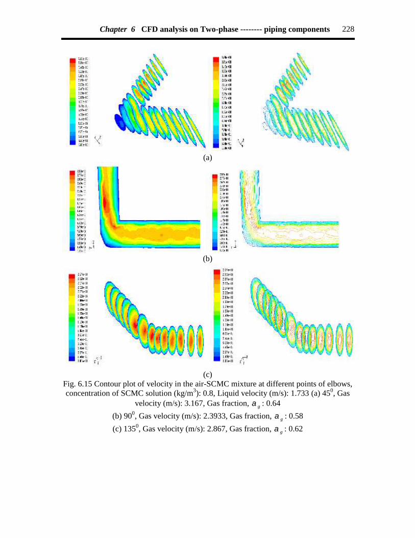
Chapter 6 CFD analysis on Two-phase -------- piping components 228
(a)
(b)
(c)Fig. 6.15 Contour plot of velocity in the air-SCMC mixture at different points of elbows,concentration of SCMC solution (kg/m3): 0.8, Liquid velocity (m/s): 1.733 (a) 450, Gas
velocity (m/s): 3.167, Gas fraction, g : 0.64
(b) 900, Gas velocity (m/s): 2.3933, Gas fraction, g : 0.58
(c) 1350, Gas velocity (m/s): 2.867, Gas fraction, g : 0.62
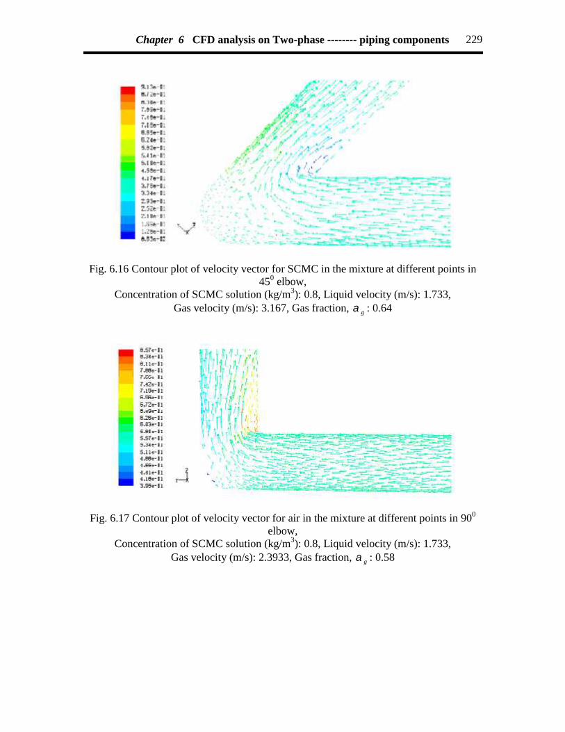
Chapter 6 CFD analysis on Two-phase -------- piping components 229
Fig. 6.16 Contour plot of velocity vector for SCMC in the mixture at different points in450 elbow,
Concentration of SCMC solution (kg/m3): 0.8, Liquid velocity (m/s): 1.733,Gas velocity (m/s): 3.167, Gas fraction, g : 0.64
Fig. 6.17 Contour plot of velocity vector for air in the mixture at different points in 900
elbow,Concentration of SCMC solution (kg/m3): 0.8, Liquid velocity (m/s): 1.733,
Gas velocity (m/s): 2.3933, Gas fraction, g : 0.58

Chapter 6 CFD analysis on Two-phase -------- piping components 230
(a)
(b)
(c)Fig. 6.18 Contours plot of static pressure for elbows, concentration of SCMC solution
(kg/m3): 0.8, Liquid velocity (m/s): 1.733 (a) 450, Gas velocity (m/s): 3.167, Gas fraction,
g : 0.64
(b) 900, Gas velocity (m/s): 2.3933, Gas fraction, g : 0.58
(c) 1350, Gas velocity (m/s): 2.867, Gas fraction, g : 0.62
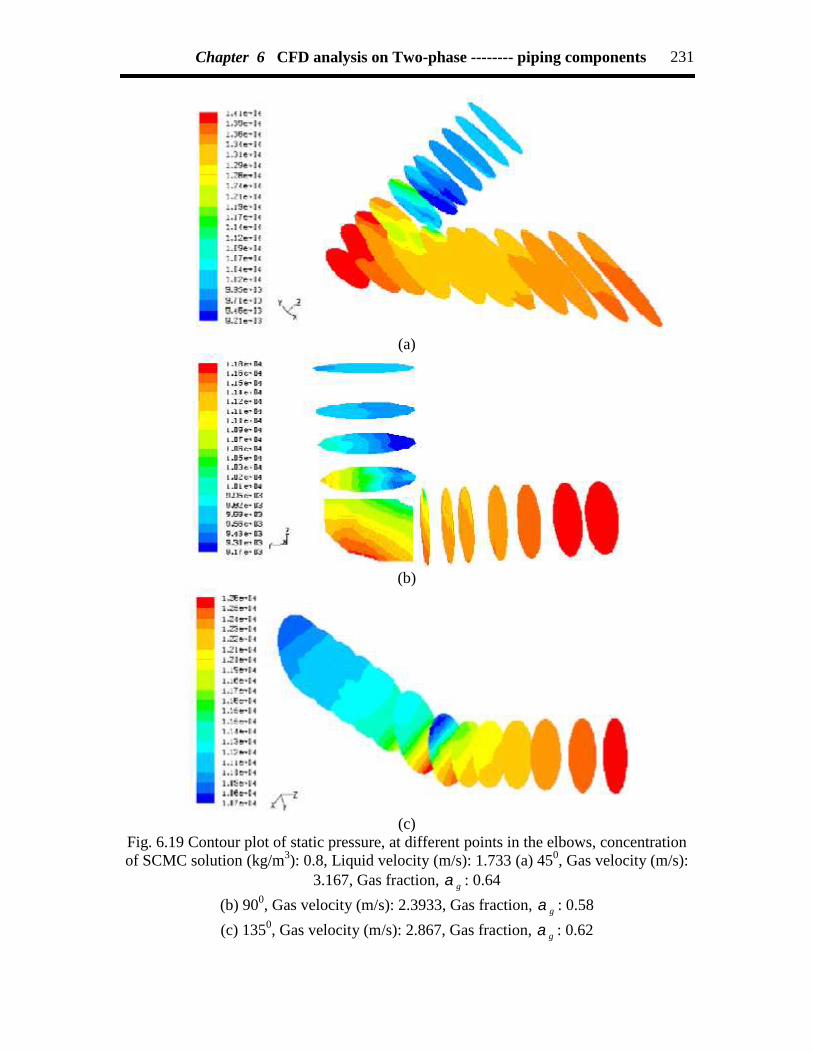
Chapter 6 CFD analysis on Two-phase -------- piping components 231
(a)
(b)
(c)Fig. 6.19 Contour plot of static pressure, at different points in the elbows, concentrationof SCMC solution (kg/m3): 0.8, Liquid velocity (m/s): 1.733 (a) 450, Gas velocity (m/s):
3.167, Gas fraction, g : 0.64
(b) 900, Gas velocity (m/s): 2.3933, Gas fraction, g : 0.58
(c) 1350, Gas velocity (m/s): 2.867, Gas fraction, g : 0.62

Chapter 6 CFD analysis on Two-phase -------- piping components 232
Fig. 6.20 Contour velocity plot inside different points of 450 elbowConcentration of SCMC solution (kg/m3): 0.8, Liquid velocity (m/s): 1.733,
Gas velocity (m/s): 3.167, Gas fraction, g : 0.64

Chapter 6 CFD analysis on Two-phase -------- piping components 233
(a) SCMC-phase
(b) air-phase
Fig. 6.21 Contours of volume fraction for 900 elbow, concentration of SCMC solution(kg/m3): 0.8, Liquid velocity (m/s): 1.733, gas velocity (m/s): 2.3933, gas fraction, g :
0.58 (a) SCMC phase and (b) air phase
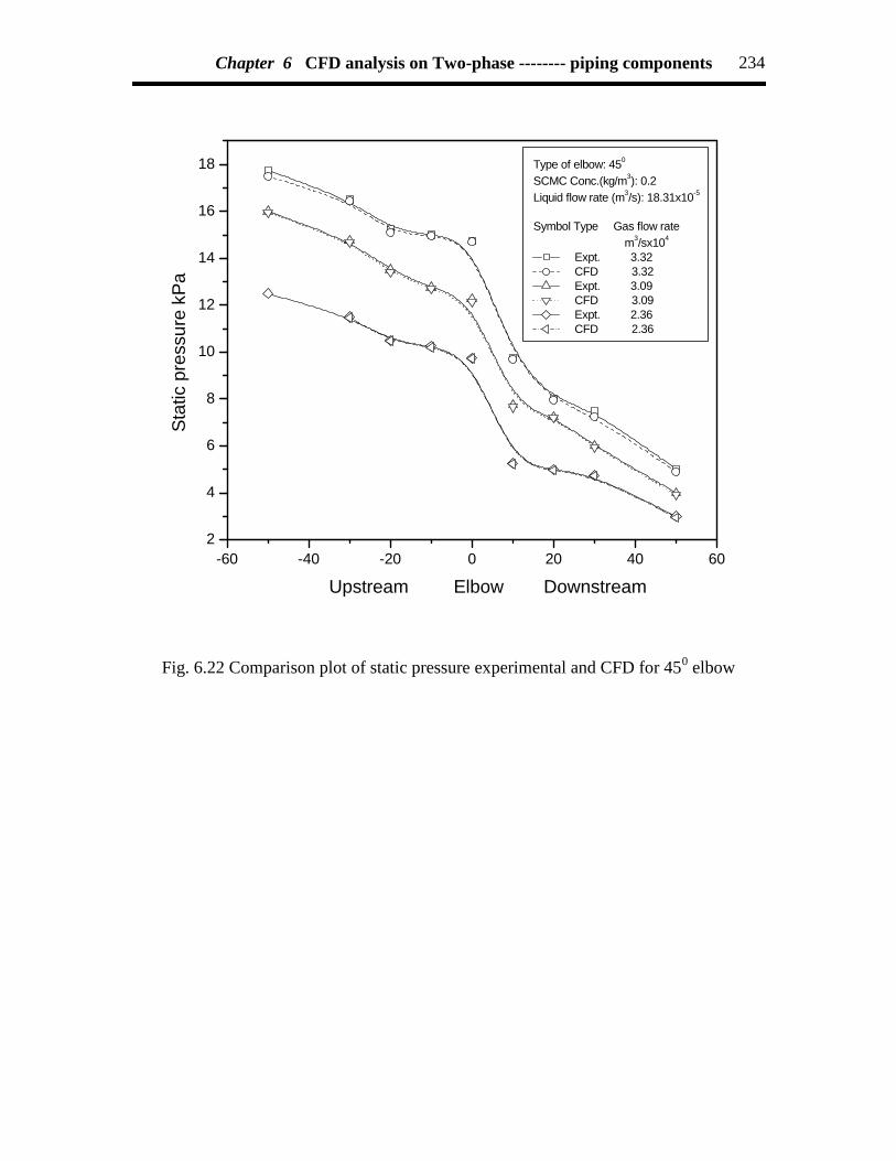
Chapter 6 CFD analysis on Two-phase -------- piping components 234
-60 -40 -20 0 20 40 602
4
6
8
10
12
14
16
18St
atic
pre
ssur
e kP
a
Upstream Elbow Downstream
Type of elbow: 450
SCMC Conc.(kg/m3): 0.2Liquid flow rate (m3/s): 18.31x10⁻⁵
Symbol Type Gas flow rate m3/sx104
Expt. 3.32 CFD 3.32 Expt. 3.09 CFD 3.09 Expt. 2.36 CFD 2.36
Fig. 6.22 Comparison plot of static pressure experimental and CFD for 450 elbow

Chapter 6 CFD analysis on Two-phase -------- piping components 235
0.2 0.4 0.6 0.8 1.0 1.2 1.4 1.6
0.2
0.4
0.6
0.8
1.0
1.2
1.4C
FD s
imul
ated
pre
ssur
e dr
op, k
Pa
Experimental pressure drop, KPa
SCMC Conc.(kg/m3): 0.2Liquid flow rate(m3/s): 3.75 x 10⁻⁵
Symbol Type 450
900
1350
Fig. 6.23 Comparison of experimental results with CFD simulated results at differentelbow angle
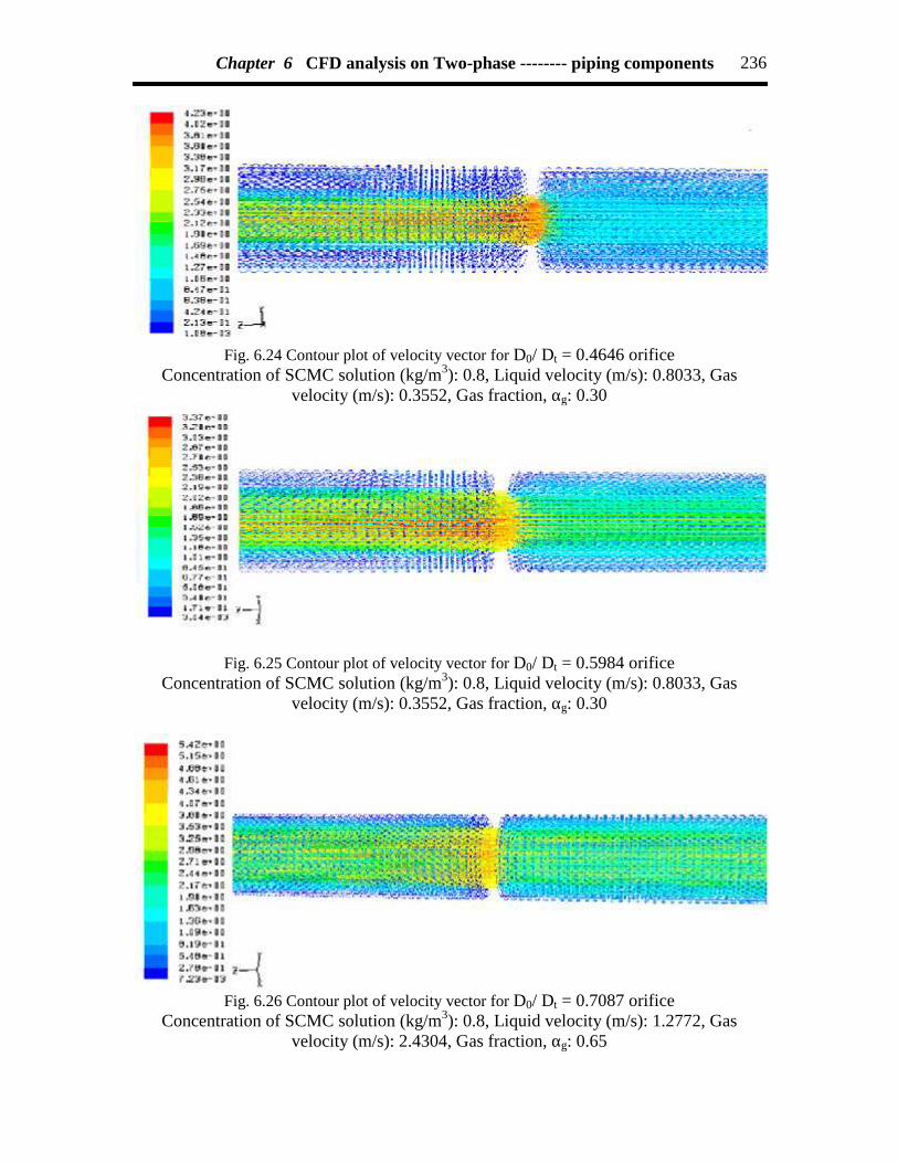
Chapter 6 CFD analysis on Two-phase -------- piping components 236
Fig. 6.24 Contour plot of velocity vector for D0/ Dt = 0.4646 orificeConcentration of SCMC solution (kg/m3): 0.8, Liquid velocity (m/s): 0.8033, Gas
velocity (m/s): 0.3552, Gas fraction, αg: 0.30
Fig. 6.25 Contour plot of velocity vector for D0/ Dt = 0.5984 orificeConcentration of SCMC solution (kg/m3): 0.8, Liquid velocity (m/s): 0.8033, Gas
velocity (m/s): 0.3552, Gas fraction, αg: 0.30
Fig. 6.26 Contour plot of velocity vector for D0/ Dt = 0.7087 orificeConcentration of SCMC solution (kg/m3): 0.8, Liquid velocity (m/s): 1.2772, Gas
velocity (m/s): 2.4304, Gas fraction, αg: 0.65
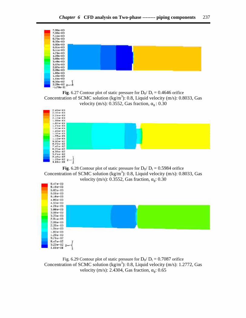
Chapter 6 CFD analysis on Two-phase -------- piping components 237
Fig. 6.27 Contour plot of static pressure for D0/ Dt = 0.4646 orificeConcentration of SCMC solution (kg/m3): 0.8, Liquid velocity (m/s): 0.8033, Gas
velocity (m/s): 0.3552, Gas fraction, αg : 0.30
Fig. 6.28 Contour plot of static pressure for D0/ Dt = 0.5984 orificeConcentration of SCMC solution (kg/m3): 0.8, Liquid velocity (m/s): 0.8033, Gas
velocity (m/s): 0.3552, Gas fraction, αg: 0.30
Fig. 6.29 Contour plot of static pressure for D0/ Dt = 0.7087 orificeConcentration of SCMC solution (kg/m3): 0.8, Liquid velocity (m/s): 1.2772, Gas
velocity (m/s): 2.4304, Gas fraction, αg: 0.65
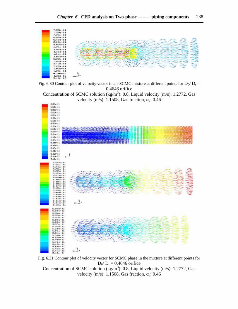
Chapter 6 CFD analysis on Two-phase -------- piping components 238
Fig. 6.30 Contour plot of velocity vector in air-SCMC mixture at different points for D0/ Dt =0.4646 orifice
Concentration of SCMC solution (kg/m3): 0.8, Liquid velocity (m/s): 1.2772, Gasvelocity (m/s): 1.1508, Gas fraction, αg: 0.46
Fig. 6.31 Contour plot of velocity vector for SCMC phase in the mixture at different points forD0/ Dt = 0.4646 orifice
Concentration of SCMC solution (kg/m3): 0.8, Liquid velocity (m/s): 1.2772, Gasvelocity (m/s): 1.1508, Gas fraction, αg: 0.46

Chapter 6 CFD analysis on Two-phase -------- piping components 239
Fig. 6.32 Contour plot of velocity vector plot of air phase in the mixture at different points forD0/ Dt = 0.4646 orifice
Concentration of SCMC solution (kg/m3): 0.8, Liquid velocity (m/s): 1.2772, Gasvelocity (m/s): 1.1508, Gas fraction, αg: 0.46

Chapter 6 CFD analysis on Two-phase -------- piping components 240
Fig. 6.33 Contours plot of velocity magnitude in the air-SCMC mixture at different points forD0/Dt = 0.4646 orifice
Concentration of SCMC solution (kg/m3): 0.8, Liquid velocity (m/s): 1.2772, Gasvelocity (m/s): 1.1508, Gas fraction, αg: 0.46

Chapter 6 CFD analysis on Two-phase -------- piping components 241
Fig. 6.34 Contours plot of velocity in the air-SCMC mixture inside the different points of D0/Dt
= 0.4646 orificeConcentration of SCMC solution (kg/m3): 0.8, Liquid velocity (m/s): 1.2772, Gas
velocity (m/s): 1.1508, Gas fraction, αg: 0.46

Chapter 6 CFD analysis on Two-phase -------- piping components 242
Fig. 6.35 Contours plot of static pressure in the air-SCMC mixture inside the different points offor D0/Dt = 0.4646 orifice
Concentration of SCMC solution (kg/m3): 0.8, Liquid velocity (m/s): 1.2772, Gasvelocity (m/s): 1.1508, Gas fraction, αg: 0.46

Chapter 6 CFD analysis on Two-phase -------- piping components 243
Fig. 6.36 Contours plot of total pressure in the air-SCMC mixture inside the different points of forD0/ Dt = 0.4646 orifice
Concentration of SCMC solution (kg/m3): 0.8, Liquid velocity (m/s): 1.2772, Gasvelocity (m/s): 1.1508, Gas fraction, αg: 0.46

Chapter 6 CFD analysis on Two-phase -------- piping components 244
Fig. 6.37 Contours of plot of SCMC phase volume fraction in the mixture inside the differentpoints of D0/Dt = 0.4646 orifice
Concentration of SCMC solution (kg/m3): 0.8, Liquid velocity (m/s): 1.2772, Gasvelocity (m/s): 1.1508, Gas fraction, αg: 0.46
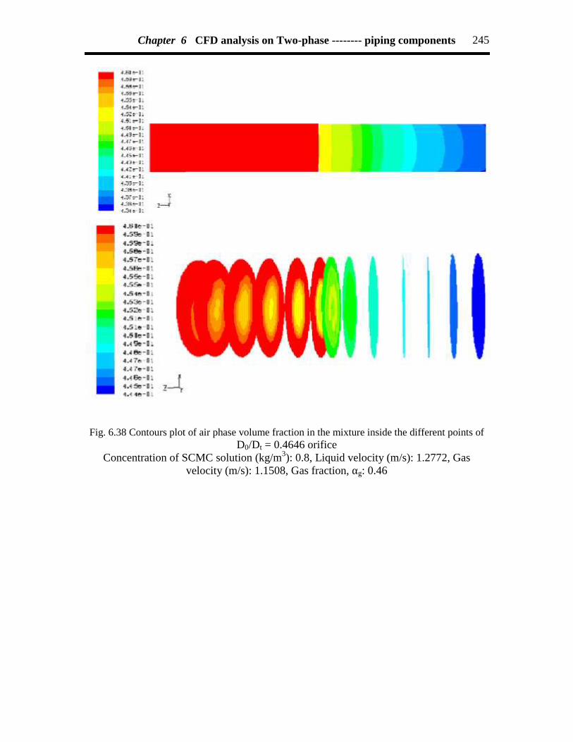
Chapter 6 CFD analysis on Two-phase -------- piping components 245
Fig. 6.38 Contours plot of air phase volume fraction in the mixture inside the different points ofD0/Dt = 0.4646 orifice
Concentration of SCMC solution (kg/m3): 0.8, Liquid velocity (m/s): 1.2772, Gasvelocity (m/s): 1.1508, Gas fraction, αg: 0.46

Chapter 6 CFD analysis on Two-phase -------- piping components 246
0 4 8 12 16 20 24 28
10
20
30
40
50
60
70
Two
- pha
se p
ress
ure
drop
, kpa
Gas flow rate, Qg x 105 m3/s
SCMC Conc.: 0.2Type of piping component: orifice, D
0/D
t: 0.4646
Symbol Type Liquid flow rate, m3/s Q
l x 10-5
Expt. 7.10 CFD 7.10 Expt. 10.17 CFD 10.17 Expt. 13.17 CFD 13.17 Expt. 16.30 CFD 16.30
Fig. 6.39 Comparison of the experimental result with CFD simulated result with differentliquid flow rate and fixed liquid concentration, fixed orifice dimension

Chapter 6 CFD analysis on Two-phase -------- piping components 247
4 8 12 16 20 24 28 32 36
5
10
15
20
25
30
35
40
45
50
55
60
65
70
75
80
Two
- pha
se p
ress
ure
drop
, kpa
Gas flow rate, Qg x 105 m3/s
Type of piping component: OrificeSCMC Conc.: 0.4 kg/m3
Liquid flow rate: 16.17 x 10⁻⁵ m3/sSymbol Type Diameter ratio D0/Dt
Expt. 0.4646 CFD 0.4646 Expt. 0.5984 CFD 0.5984 Expt. 0.7087 CFD 0.7087
Fig. 6.40 Comparison of the experimental result with CFD simulated result with differentorifice dimension and fixed liquid concentration, fixed liquid flow rate

Chapter 6 CFD analysis on Two-phase -------- piping components 248
10 15 20 25 30 35 40
10
15
20
25
30
35
40
CFD
sim
ulat
ed p
ress
ure
drop
, kPa
Experimental pressure drop, kPa
Scmc concentration(kg/m3):0.2Type of piping component: Orifice D0/Dt:0.4646Symbol Type Liquid flow rate Qlx105, m3/s
7.10 10.17 13.17 16.30
Fig. 6.41 Comparison of experimental results with CFD simulated results for differentliquid flow rates

Chapter 6 CFD analysis on Two-phase -------- piping components 249
5 10 15 20 25 30 35 40 45
5
10
15
20
25
30
35
40
45C
FD s
imul
ated
pre
ssur
e dr
op, k
Pa
Experimental pressure drop, kPa
SCMC concentration(kg/m3):0.4Type of piping component:OrificeLiquid flow rate(3/s):16.17x10-5
Symbol Type D0/Dt
0.4646 0.5984 0.7087
Fig. 6.42 Comparison of experimental results with CFD simulated results for differentorifice diameter ratios
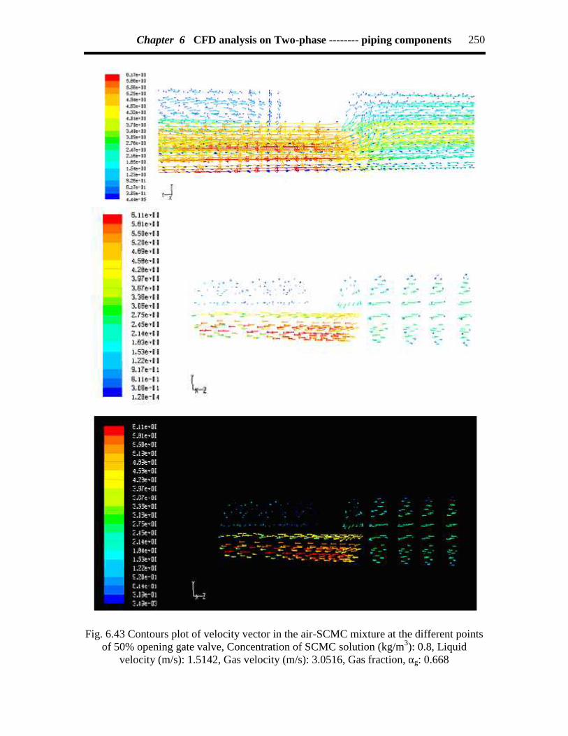
Chapter 6 CFD analysis on Two-phase -------- piping components 250
Fig. 6.43 Contours plot of velocity vector in the air-SCMC mixture at the different pointsof 50% opening gate valve, Concentration of SCMC solution (kg/m3): 0.8, Liquid
velocity (m/s): 1.5142, Gas velocity (m/s): 3.0516, Gas fraction, αg: 0.668

Chapter 6 CFD analysis on Two-phase -------- piping components 251
Fig. 6.44 Contours plot of velocity magnitude in the air-SCMC mixture at the differentpoints of 50% opening gate valve, Concentration of SCMC solution (kg/m3): 0.8, Liquid
velocity (m/s): 1.5142, Gas velocity (m/s): 3.0516, Gas fraction, αg: 0.6683

Chapter 6 CFD analysis on Two-phase -------- piping components 252
Fig. 6.45 Contours plot of velocity in the air-SCMC mixture at the different points of50% opening gate valve, Concentration of SCMC solution (kg/m3): 0.8, Liquid velocity
(m/s): 1.5142, Gas velocity (m/s): 3.0516, Gas fraction, αg: 0.6683

Chapter 6 CFD analysis on Two-phase -------- piping components 253
Fig. 6.46 Contours plot of static pressure in the air-SCMC mixture at the different pointsof 50% opening gate valve, Concentration of SCMC solution (kg/m3): 0.8, Liquid
velocity (m/s): 1.5142, Gas velocity (m/s): 3.0516, Gas fraction, αg: 0.6683
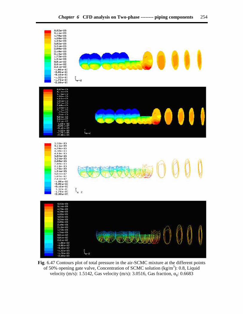
Chapter 6 CFD analysis on Two-phase -------- piping components 254
Fig. 6.47 Contours plot of total pressure in the air-SCMC mixture at the different pointsof 50% opening gate valve, Concentration of SCMC solution (kg/m3): 0.8, Liquid
velocity (m/s): 1.5142, Gas velocity (m/s): 3.0516, Gas fraction, αg: 0.6683
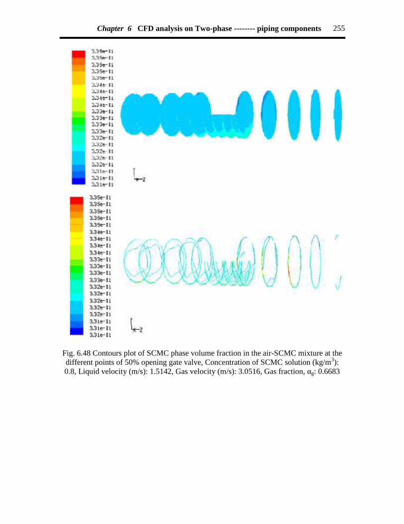
Chapter 6 CFD analysis on Two-phase -------- piping components 255
Fig. 6.48 Contours plot of SCMC phase volume fraction in the air-SCMC mixture at thedifferent points of 50% opening gate valve, Concentration of SCMC solution (kg/m3):0.8, Liquid velocity (m/s): 1.5142, Gas velocity (m/s): 3.0516, Gas fraction, αg: 0.6683

Chapter 6 CFD analysis on Two-phase -------- piping components 256
Fig. 6.49 Contours plot of air phase volume fraction in the air-SCMC mixture at thedifferent points of 50% opening gate valve, Concentration of SCMC solution (kg/m3):0.8, Liquid velocity (m/s): 1.5142, Gas velocity (m/s): 3.0516, Gas fraction, αg: 0.6683

Chapter 6 CFD analysis on Two-phase -------- piping components 257
2.0 2.5 3.0 3.5 4.0 4.5 5.0
2.0
2.5
3.0
3.5
4.0
4.5
5.0
CFD
sim
ulat
ed p
ress
ure
drop
Experimental pressure drop, kPa
SCMC concentration(kg/m3): 0.2Type of piping component:50% opening Gate valveSymbol Type Liquid flow rate Qlx105, m3/s
7.25 9.08 10.83 12.58
Fig. 6.50 Comparison of experimental results with CFD simulated results for differentliquid flow rates

Chapter 6 CFD analysis on Two-phase -------- piping components 258
2 4 6 8 10
2
4
6
8
10C
FD s
imul
ated
pre
sure
dro
p, k
Pa
Experimental pressure drop, kPa
SCMC concentration(kg/m3):0.2Type of piping component:Gate valveLiquid flow rate(m3/s):15.83x10-5
Symbol Type 50 75 100
Fig.6.51 Comparison of experimental results with CFD simulated results for different %opening of Gate valve

Chapter 6 CFD analysis on Two-phase -------- piping components 259
Fig. 6.52 Contours plot of velocity vector in the air-SCMC mixture for 50% openingglobe valve, Concentration of SCMC solution (kg/m3): 0.8, Liquid velocity (m/s): 1.5142,
Gas velocity (m/s): 1.7265, Gas fraction, αg: 0.5

Chapter 6 CFD analysis on Two-phase -------- piping components 260
Fig. 6.53 Contours plot of velocity vector in the air-SCMC mixture at the different pointsof 50% opening globe valve, Concentration of SCMC solution (kg/m3): 0.8, Liquid
velocity (m/s): 1.5142, Gas velocity (m/s): 1.7265, Gas fraction, αg: 0.5

Chapter 6 CFD analysis on Two-phase -------- piping components 261
Fig. 6.54 Contours plot of velocity vector for SCMC phase in the air-SCMC mixture atthe different points of 50% opening globe valve, Concentration of SCMC solution
(kg/m3): 0.8, Liquid velocity (m/s): 1.5142, Gas velocity (m/s): 1.7265, Gas fraction, αg:0.5

Chapter 6 CFD analysis on Two-phase -------- piping components 262
Fig. 6.55 Contours plot of velocity vector for air phase in the air-SCMC mixture at thedifferent points of 50% opening globe valve, Concentration of SCMC solution (kg/m3):
0.8, Liquid velocity (m/s): 1.5142, Gas velocity (m/s): 1.7265, Gas fraction, αg: 0.5

Chapter 6 CFD analysis on Two-phase -------- piping components 263
Fig. 6.56 Contours plot of velocity magnitude in the air-SCMC mixture at the differentpoints of 50% opening globe valve, Concentration of SCMC solution (kg/m3): 0.8,
Liquid velocity (m/s): 1.5142, Gas velocity (m/s): 1.7265, Gas fraction, αg: 0.5

Chapter 6 CFD analysis on Two-phase -------- piping components 264
Fig. 6.57 Contours plot of axial velocity in the air-SCMC mixture at the different pointsof 50% opening globe valve, Concentration of SCMC solution (kg/m3): 0.8, Liquid
velocity (m/s): 1.5142, Gas velocity (m/s): 1.7265, Gas fraction, αg: 0.5

Chapter 6 CFD analysis on Two-phase -------- piping components 265
Fig. 6.58 Contours plot of static pressure in the air-SCMC mixture at the different pointsof 50% opening globe valve, Concentration of SCMC solution (kg/m3): 0.8, Liquid
velocity (m/s): 1.5142, Gas velocity (m/s): 1.7265, Gas fraction, αg: 0.5
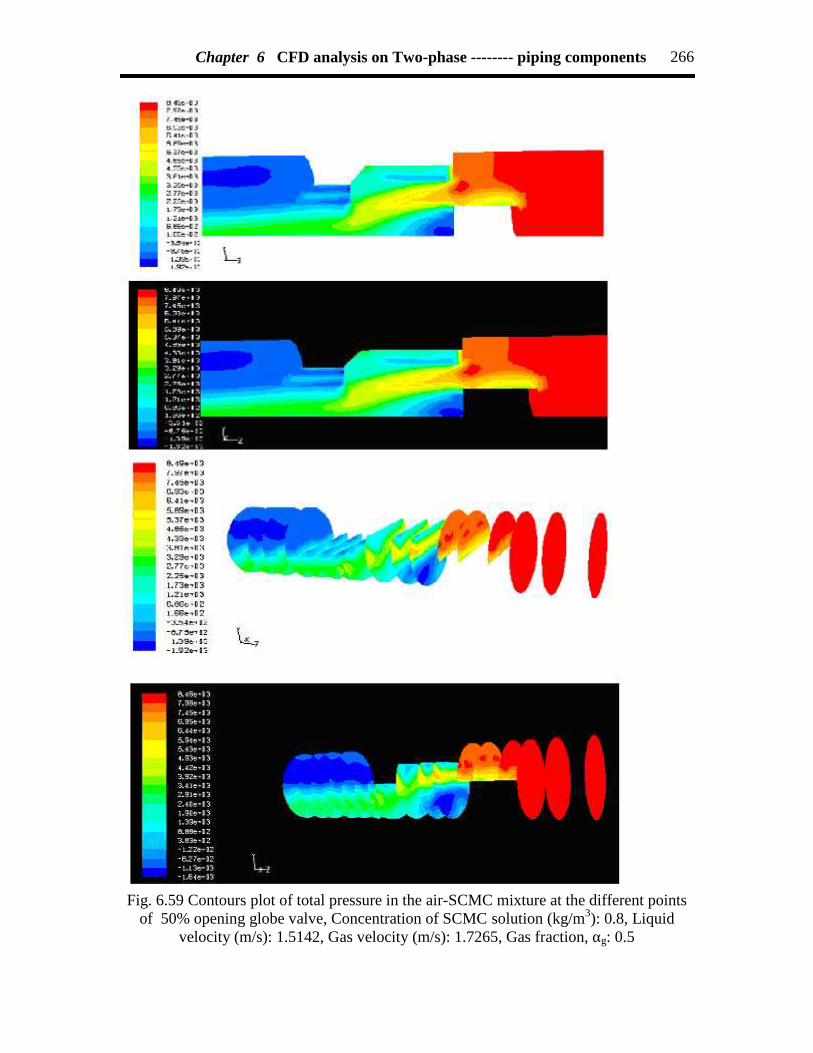
Chapter 6 CFD analysis on Two-phase -------- piping components 266
Fig. 6.59 Contours plot of total pressure in the air-SCMC mixture at the different pointsof 50% opening globe valve, Concentration of SCMC solution (kg/m3): 0.8, Liquid
velocity (m/s): 1.5142, Gas velocity (m/s): 1.7265, Gas fraction, αg: 0.5

Chapter 6 CFD analysis on Two-phase -------- piping components 267
Fig. 6.60 Contours plot of SCMC phase volume fraction in the air-SCMC mixture at thedifferent points of 50% opening globe valve, Concentration of SCMC solution (kg/m3):
0.8, Liquid velocity (m/s): 1.5142, Gas velocity (m/s): 1.7265, Gas fraction, αg: 0.5

Chapter 6 CFD analysis on Two-phase -------- piping components 268
Fig. 6.61 Contours plot of air phase volume fraction in the air-SCMC mixture at thedifferent points of 50% opening globe valve, Concentration of SCMC solution (kg/m3):
0.8, Liquid velocity (m/s): 1.5142, Gas velocity (m/s): 1.7265, Gas fraction, αg: 0.5

Chapter 6 CFD analysis on Two-phase -------- piping components 269
5 10 15 20 25 30 35 40
5
10
15
20
25
30
35
40
Two
- pha
se p
ress
ure
drop
, kpa
Gas flow rate, Qg x 105 m3/s
SCMC Conc.: 0.2 kg/m3
Type of piping component: 50% opening Globe ValveSymbol Type Liquid flow rate m3/s Q
l x 10-5
Expt. 4.05 CFD 4.05 Expt. 7.25 CFD 7.25 Expt. 10.83 CFD 10.83 Expt. 14.33 CFD 14.33
Fig. 6.62 Comparison of experimental and CFD simulated result at different liquid flowrate and fixed liquid concentration, fixed opening of the Globe valve

Chapter 6 CFD analysis on Two-phase -------- piping components 270
4 6 8 10 12 14 16 18 20 22 24
4
6
8
10
12
14
16
18
20
22C
FD s
imul
ated
pre
ssur
e dr
op, k
Pa
Experimental pressure drop, kPa
SCMC concentration(kg/m3):0.2Type of piping component:50 % opening Globe valveSymbol Type
4.05 7.25 10.83 14.33
Fig. 6.63 Comparison of experimental results with CFD simulated results for differentliquid flow rates

Chapter 6 CFD analysis on Two-phase -------- piping components 271
14 16 18 20 22 2412
14
16
18
20
22C
FD s
imul
ated
pre
ssur
e dr
op, k
Pa
Experimental pressure drop, kPa
SCMC concentration(kg/m3):0.2Type of piping component: Globe valveLiquid flow rate(m3/s):14.33x10-5
Symbol % opening of valve 50 75 100
Fig. 6.64 Comparison of experimental results with CFD simulated results for different %opening of Globe valve

Chapter 6 CFD analysis on Two-phase -------- piping components 272
Table 6.1 Range of variables
Measurement Type RangeLiquid and Flow properties
Flow behavior index 0.6015 ≤ n/ ≤ 0.9013Consistency index (Nsn'/m2) 0.0142 ≤ K/ ≤ 0.7112
Density (kg/m3) 1001.69 ≤ ρ ≤ 1003.83Concentration of SCMC Solution
(kg/m3)0.2 to 0.8
Liquid Flow Rate Ql×105(m3/s) 3.75 to 29.83Gas Flow Rate Qg×105(m3/s) 2.90 to 44.75
Reynolds Number 47.51 ≤ Re ≤ 2234.21Dean Number 32.41 ≤ De ≤ 2130.23
Pressure Drop (Experimental) (kPa) 0.1333 ≤ ΔP ≤ 45.46Elbow
Angle of Elbow 45° to 135°
450 elbow Radius of curvature = 0.011mLinear length of the elbow = 0.014m
900 elbow Radius of curvature = 0.022mLinear length of the elbow = 0.011m
1350 elbow Radius of curvature = 0.017mLinear length of the elbow = 0.016m
OrificeDiameter of Orifice (m) 0.0059, 0.0038, 0.0045
Diameter ratio of Orifice to pipediameter
0.4646 ≤ D0/Dt ≤ 0.7087
Gate valve
Valve opening (%) 50, 75, 100
Ratio of the valve opening to the fullopening of valve
0.50≤ α ≤ 1.00
Globe ValveValve opening (%) 50, 75, 100
Ratio of the valve opening to the fullopening of valve
0.50≤ α ≤ 1.00

Chapter 6 CFD analysis on Two-phase -------- piping components 273
Table 6.2
Comparison of the experimental and CFD analysis data of two-phase pressure dropthrough straight pipe for different flow rate
Sl.No.
Air flow rate
Ql x 105
m3/s
Two-phasepressure
drop,experimental
( tpP )
Straightpipe, Expt.
kPa
Two-phasepressure drop,
CFD
( tpP )
straightpipe, CFD
kPaLiquid flow rate, Ql : 4.05 x 10⁻⁵ m3/s; SCMC
Concentration(kg/m3): 0.21 3.1 2.6 2.552 6.13 3.6 3.453 11.68 4.6 4.564 15.78 4.73 4.655 19.21 5.66 5.6
Liquid flow rate, Ql : 7.00 x 10⁻⁵ m3/s; SCMCConcentration(kg/m3): 0.2
6 5.43 4.35 4.257 8.56 4.85 4.758 11.21 5.7 5.659 15.85 5.8 5.75
10 20.98 6.75 6.66Liquid flow rate, Ql : 9.80 x 10⁻⁵ m3/s; SCMC
Concentration(kg/m3): 0.211 9.09 6.65 6.612 11.4 7.5 7.4513 15.67 8.88 8.8514 21.09 9.95 9.915 23.54 10.56 10.35
Liquid flow rate, Ql : 13.17 x 10⁻⁵ m3/s; SCMCConcentration(kg/m3): 0.2
16 5.76 8.5 8.417 9.65 9.95 9.818 12.18 11.18 1119 15.78 12 11.8620 19.28 13.75 13.55

Chapter 6 CFD analysis on Two-phase -------- piping components 274
Table 6.3
Comparison of the experimental and CFD analysis data of two-phase pressure dropthrough straight pipe for different SCMC concentration
Sl.No.
Air flow rate
Ql x 105
m3/s
Two-phasepressure
drop,experimental
( tpP )
Straightpipe, Expt.
kPa
Two-phasepressure drop,
CFD
( tpP )
Straight pipe,CFD
kPaLiquid flow rate, Ql : 7.00 x 10⁻⁵ m3/s; SCMC
Concentration(kg/m3): 0.21 5.43 4.35 4.252 8.56 4.85 4.753 11.21 5.7 5.654 15.85 5.8 5.755 20.98 6.75 6.66
Liquid flow rate, Ql : 7.00 x 10⁻⁵ m3/s; SCMCConcentration(kg/m3): 0.4
6 9.44 6.7 6.657 13.21 8.6 8.458 15.19 9.2 8.959 18.21 10.7 10.5
10 20.63 11.5 11.35Liquid flow rate, Ql : 7.00 x 10⁻⁵ m3/s; SCMC
Concentration(kg/m3): 0.611 6.15 6.95 6.8512 7.28 7.69 7.6513 12.44 8.85 8.4514 13.15 9.5 9.3515 18.86 11.83 11.65
Liquid flow rate, Ql : 7.00 x 10⁻⁵ m3/s; SCMCConcentration(kg/m3): 0.8
16 5.98 7.55 7.4517 12.09 9.56 9.418 17.56 12.65 12.519 22.22 13.5 13.44

Chapter 6 CFD analysis on Two-phase -------- piping components 275
Table 6.4
Comparison of the experimental and CFD analysis data of two-phase pressure dropthrough elbows for different liquid flow rate
Sl.No.
Air flow rate
Ql x 105
m3/s
Two-phasepressure
drop,experimental
( tpP )
elbow, Expt.
kPa
Two-phasepressure drop,
CFD
( tpP )
elbow, CFD
kPaType of elbow: 450, Liquid flow rate, Ql : 3.75 x 10⁻⁵ m3/s;
SCMC Concentration(kg/m3): 0.21 0.153 0.4 0.3852 0.193 0.4667 0.453 0.251 0.6667 0.654 0.351 0.9333 0.925 0.385 1.4667 1.4
Type of elbow: 450, Liquid flow rate, Ql : 11.00 x 10⁻⁵ m3/s;SCMC Concentration(kg/m3): 0.2
6 0.147 1.2 1.127 0.215 1.333 1.328 0.261 1.4667 1.459 0.287 1.7333 1.7
10 0.328 2.5333 2.5Type of elbow: 450, Liquid flow rate, Ql : 14.62 x 10⁻⁵ m3/s;
SCMC Concentration(kg/m3): 0.211 0.052 1.4667 1.4512 0.121 2.2 2.1213 0.157 2.2667 2.214 0.186 2.4667 2.4515 0.271 2.6667 2.6

Chapter 6 CFD analysis on Two-phase -------- piping components 276
Table 6.5
Comparison of the experimental and CFD analysis data of two-phase pressure dropthrough elbows at different elbow angle
Sl.No.
Air flow rate
Ql x 105
m3/s
Two-phasepressure
drop,experimental
( tpP )
elbow, Expt.
kPa
Two-phasepressure drop,
CFD
( tpP )
elbow, CFD
kPa
Type of elbow: 450, Liquid flow rate, Ql : 3.75 x 10⁻⁵ m3/s;SCMC Concentration(kg/m3): 0.2
1 0.153 0.4 0.3852 0.193 0.4667 0.453 0.251 0.6667 0.654 0.351 0.9333 0.925 0.385 1.4667 1.4
Type of elbow: 900, Liquid flow rate, Ql : 3.75 x 10⁻⁵ m3/s;SCMC Concentration(kg/m3): 0.2
6 0.032 0.2 0.187 0.121 0.4667 0.458 0.16 0.5333 0.59 0.226 0.6667 0.65
10 0.313 0.7333 0.72Type of elbow: 1350, Liquid flow rate, Ql : 3.75 x 10⁻⁵
m3/s; SCMC Concentration(kg/m3): 0.211 0.037 0.2667 0.2512 0.289 0.4667 0.4513 0.342 0.5333 0.514 0.355 0.6667 0.6215 0.385 0.8 0.75

Chapter 6 CFD analysis on Two-phase -------- piping components 277
Table 6.6
Comparison of the experimental and CFD analysis data of two-phase pressure dropthrough orifices at different liquid flow rate
Sl.No.
Air flow rate
Ql x 105
m3/s
Two-phasepressure
drop,experimental
( tpP )
orifice, Expt.
kPa
Two-phasepressure drop,
CFD
( tpP ) orifice,
CFD
kPaOrifice : D0/ Dt = 0.4646, Liquid flow rate, Ql : 7.10 x 10⁻⁵
m3/s; SCMC Concentration(kg/m3): 0.21 9.329 6.6667 6.62 11.509 7.8667 7.73 15.075 8 7.54 15.923 8 7.85 17.064 8.8 8.56 26.292 9.0667 8.78
Orifice : D0/ Dt = 0.4646, Liquid flow rate, Ql : 10.17 x 10⁻⁵
m3/s; SCMC Concentration(kg/m3): 0.27 8.327 14.5333 14.58 12.021 14.6667 14.69 12.549 16 15.5
10 14.996 16.4 1611 17.631 17.3333 1712 22.944 17.3333 17.5
Orifice : D0/ Dt = 0.4646, Liquid flow rate, Ql : 13.17 x 10⁻⁵
m3/s; SCMC Concentration(kg/m3): 0.213 10.053 20.8 2014 10.81 22 21.515 11.634 22.2667 2216 13.392 23.8667 23.517 15.213 24.1333 2418 19.255 25.4667 25
Orifice : D0/ Dt = 0.4646, Liquid flow rate, Ql : 16.30 x 10⁻⁵
m3/s; SCMC Concentration(kg/m3): 0.219 4.456 23.6 2320 12.804 34 3321 12.815 34.1333 33.522 15.163 35.8667 34.523 17.301 38.5332 3824 18.132 39.3332 39

Chapter 6 CFD analysis on Two-phase -------- piping components 278
Table 6.7
Comparison of the experimental and CFD analysis data of two-phase pressure dropthrough orifices at different orifice diameter ratio
Sl.No.
Air flow rate
Ql x 105
m3/s
Two-phasepressure
drop,experimental
( tpP )
orifice, Expt.
kPa
Two-phasepressure drop,
CFD
( tpP ) orifice,
CFD
kPaOrifice : D0/ Dt = 0.4646, Liquid flow rate, Ql : 16.17 x 10⁻⁵
m3/s; SCMC Concentration(kg/m3): 0.41 7.13 28.93 28.22 9.19 32.93 32.353 10.15 33.73 33.264 12.86 37.33 36.845 15.76 40 39.256 15.85 39.46 397 18.14 43.33 42.98 22.66 44.4 44.21
Orifice : D0/ Dt = 0.5984, Liquid flow rate, Ql : 16.17 x 10⁻⁵
m3/s; SCMC Concentration(kg/m3): 0.49 5.11 9.46 9.11
10 11.7 11.33 10.7611 12.41 12.26 11.6112 16.81 12.53 11.7313 20 14.13 13.8714 23.7 15.86 15.2415 29.26 15.73 15.3416 31.66 16.4 15.9117 14.44 5.2 4.518 17.5 5.2 4.7819 31.47 7.6 7.1720 33.29 13 12.6521 37.15 13.33 12.81

Chapter 6 CFD analysis on Two-phase -------- piping components 279
Table 6.8Comparison of the experimental and CFD analysis data of two-phase pressure drop
through gate valve at different flow rate
Sl.No.
Air flow rate
Ql x 105
m3/s
Two-phasepressure
drop,experimental
( tpP ) gate
valve, Expt.
kPa
Two-phasepressure drop,
CFD
( tpP )gate valve,
CFD
kPaGate Valve : 50% opening, Liquid flow rate, Ql : 7.25 x 10-
5 m3/s; SCMC Concentration(kg/m3): 0.21 14.25 1.8667 1.752 18.55 2.1333 2
Gate Valve : 50% opening, Liquid flow rate, Ql : 9.08 x 10-
5 m3/s; SCMC Concentration(kg/m3): 0.23 11.98 2 1.854 17.08 2 1.95 19.52 2 1.956 20.29 1.733 27 36.14 2.933 2.74
Gate Valve : 50% opening, Liquid flow rate, Ql : 10.83 x10⁻⁵ m3/s; SCMC Concentration(kg/m3): 0.2
8 13.43 2.666 2.69 16.46 2.4 2.3
10 23.21 2.533 2.4511 35.82 2.666 2.55
Gate Valve : 50% opening, Liquid flow rate, Ql : 12.58 x10⁻⁵ m3/s; SCMC Concentration(kg/m3): 0.2
12 8.21 2.666 2.6213 11 2.5333 2.4814 16 3.2 315 19.41 3.2 3.116 24.77 3.333 3.2517 37.25 4.9333 4.75
Gate Valve : 50% opening, Liquid flow rate, Ql : 14.33 x10⁻⁵ m3/s; SCMC Concentration(kg/m3): 0.2
18 9 2.9333 2.8519 10.62 3.2 3.120 13.37 2.9333 2.921 13.56 3.6 3.522 16.53 4 3.9523 23.21 4.133 4.124 40.5 4.8 4.6

Chapter 6 CFD analysis on Two-phase -------- piping components 280
Table 6.9
Comparison of the experimental and CFD analysis data of two-phase pressure drop atdifferent opening of gate valve
Sl.No.
Air flow rate
Ql x 105
m3/s
Two-phasepressure
drop,experimental
( tpP ) gate
valve, Expt.
kPa
Two-phasepressure drop,
CFD
( tpP )gate valve,
CFD
kPaGate Valve : 50% opening, Liquid flow rate, Ql : 15.83 x
10-5 m3/s; SCMC Concentration(kg/m3): 0.21 9.23 3.8667 3.752 12.08 4.5333 4.453 14.12 4.5333 4.54 20.11 4.8 4.75 26.84 4.8 4.756 40.59 9.3333 9.85
Gate Valve : 75% opening, Liquid flow rate, Ql : 15.83 x10⁻⁵ m3/s; SCMC Concentration(kg/m3): 0.2
7 8.24 2 1.988 10.49 3.0667 39 12.6 2.9333 2.8
10 14.45 2.9333 2.8511 19.84 4.1333 412 26.18 4.6667 4.55
Gate Valve : 100% opening, Liquid flow rate, Ql : 15.83 x10⁻⁵ m3/s; SCMC Concentration(kg/m3): 0.2
13 5.514 1.8667 1.814 8.324 1.7333 1.6515 11.655 2 1.916 17.198 2.2667 2.217 22.831 3.6 3.55

Chapter 6 CFD analysis on Two-phase -------- piping components 281
Table 6.10
Comparison of the experimental and CFD analysis data of two-phase pressure drop atdifferent opening of globe valve
Sl.No.
Air flow rate
Ql x 105
m3/s
Two-phasepressure
drop,experimental
( tpP ) globe
valve, Expt.
kPa
Two-phasepressure drop,
CFD
( tpP )globe valve,
CFD
kPaGlobe Valve : 50% opening, Liquid flow rate, Ql : 14.33 x
10-5 m3/s; SCMC Concentration(kg/m3): 0.21 8.05 16.53 16.252 14.66 18.8 18.73 18.33 19.73 19.654 29.65 22.8 22.55 36.33 23.06 22.75
Globe Valve : 75% opening, Liquid flow rate, Ql : 14.33 x10⁻⁵ m3/s; SCMC Concentration(kg/m3): 0.2
6 9.72 14.66 14.57 13.62 14.8 14.78 17.88 17.2 179 18.66 14.8 14.5
10 24.45 17.06 17.7511 30.49 18.13 1812 36.73 20 19.5
Globe Valve : 100% opening, Liquid flow rate, Ql : 14.33 x10⁻⁵ m3/s; SCMC Concentration(kg/m3): 0.2
13 9.43 12.93 12.814 11.58 14 13.815 16.08 15.2 1516 16.08 14.53 15.317 16.62 14.66 15.518 20.27 16.13 1619 24.59 16.26 16.1220 30.2 17.2 1721 34.28 18 17.5

Chapter 7
Non-Newtonian liquid flow through helical coils – CFD analysis
Chapter 7 Non-Newtonian liquid flow through helical coil – CFD analysis 283
Experimental investigation has been carried out for non-Newtonian liquid flow
through helical coils. The Computational Fluid Dynamics (CFD) analysis using Fluent
6.3 software evaluates the frictional pressure drop across the helical coils. The CFD
results compare with the experimental data.
7.1 Introduction
Helical coils are extensively used in compact heat exchangers, heat exchanger
networks, heating or cooling coils in piping systems, intake in air crafts, fluid amplifiers,
coil steam generators, refrigerators, nuclear reactors, thermosiphones, other heat-transfer
equipment and chemical plants, as well as in the food and drug industries. But non-
Newtonian fluid flows through helical coils are mainly used in pulp and paper, paints,
tooth-paste industries. One of the main advantages in the use of helical coiled tubes as
chemical reactors or heat exchangers lies in the fact that considerable lengths of tubing
can be contained in a space-saving configuration that can easily be placed in a
temperature-controlled environment. The heat and mass transfer coefficients in helical
coiled tubes are higher than those in straight tubes. When fluid flows through a curved
pipe, the presence of curvature generates a centrifugal force that acts at right angles to the
main flow, resulting in secondary flow. The strength of the secondary flow depends on
the curvature of the surface. A literature survey indicates that numerous studies dealing
with flow phenomena and pressure drop in single-phase flow through helical coils have
been published. These are well summarized in Berger et al. (1983), Shah and Joshi
(1987) and Das (1996). Coiled tubes are basically Dean-vortex-based systems, in which
the curvature directly induces secondary flows to enhance the radial mixing. The
formation of centrifugal instabilities in the flow creates higher vorticity and also shear
Chapter 7 Non-Newtonian liquid flow through helical coil – CFD analysis 284
rates at the wall of the coil thus stronger mixing effect generates than the normal Taylor
vortices (Tiwari et al. 2004; Gelfgat et al., 2003). The use of Dean vortices were utilized
in the various membrane module configuration. U-bend and helical tubes are the most
commonly used geometries (So et al., 1991; Chung et al., 1996; Yamamoto et al., 1994;
Moulin et al., 2001, etc.). Moulin et al. (2001) studied the wall shear stress by using four
types of tube geometry, i.e., straight, torus, helical and woven, and concluded that the
helical geometry gives more wall shear stress. Guan and Martonen (2000) simulated by
using CFD to observed the developing length of velocity patterns and transitional
character of fluid flowing in curved geometry.
In order to achieve optimum performance, an accurate design technique is
necessary for the prediction of two–phase pressure drop through helical coil tube. This
chapter deals with the computational fluid dynamics technique, FLUENT 6.3, to predict
the pressure drop in helical coil tubes.
7.2 The experimental setup
The detail experimental set up is shown in Fig. 7.1. The experimental apparatus
consisted of a solution tank, heat exchanger, centrifugal pumps, a test section, control and
measuring systems for flow rate, pressure drop and other accessories.
The liquid storage tank was a cylindrical vessel of 0.45 m3 capacity and was fitted
with a propeller type of stirrer for uniform mixing of sodium salt of carboxymethyl
cellulose (SCMC) solutions. The test liquids were prepared by dissolving the required
amount of SCMC in tap water, stirring until a homogeneous solution was obtained and
kept around 15hr. for aging. Adding trace amounts of formalin prevented biological

Chapter 7 Non-Newtonian liquid flow through helical coil – CFD analysis 285
degradation. Content of the tank was kept at a constant temperature by circulating water
through a copper coil.
Thick walled flexible, transparent PVC pipes with internal diameter of 0.00933 –
0.01200 m having the total length of the tube as 15 m was used as experiment. The PVC
pipes were wound round a cylindrical hard PVC frame of known diameter to form a
helical coil. The helical coils were fixed and carefully tightened with clamps in order to
avoid deformation of the tube. Changing the diameter of the frame and diameter of the
tube will vary coil diameter. The tubes were wound in closed packed fashion so that the
pitch is equal to the outer diameter of the tube and maintained constant for all cases.
Helix angle of 00 was used for experiment. The entire test section was vertically mounted
on frame to prohibit vibration. Detailed dimensions of the coils used in the experiments
are given in Table 7.1.
The test liquid was circulated from the tank by means of a centrifugal pump to the
helical coil test section. Its flow rate was controlled by bypass valves and was measured
by a set of rotameters (RL1 and RL2) [Transducers and Controls Pvt. Ltd., Hyderabad,
India, Accuracy ±2%] connected in parallel. The liquid was discharged in the level
control tank and was returned to the liquid storage tank.
The level control tank diameter 0.25 m and height 0.6 m was made from mild
steel sheet. The liquid level in the level control tank was always kept below the test
section. The level of liquid in the control tank was controlled with the help of a level
controller.
The pressure taps were located at the middle of the vertical helical coils. The
upstream pressure tap was mounted after 4 to 6 coil turns in order to reduce the effect of

Chapter 7 Non-Newtonian liquid flow through helical coil – CFD analysis 286
the upstream flow and downstream pressure tap also mounted before 4 to 6 coils turns to
reduce the down stream flow. The two pressure tap were adjusted to ensure that they
were on the same vertical line. A simple U-tube manometer containing mercury beneath
the water measured the pressure difference.
Four aqueous solutions of SCMC (Loba Cheme Pvt. Ltd., Mumbai, India) of
approximate concentrations 0.2 kg/m3, 0.4 kg/m3, 0.6 kg/m3 and 0.8 kg/m3, were used as
non-Newtonian liquids. The properties of the non-Newtonian liquids were measured by
standard techniques, i.e., viscosity was measured by pipeline viscometer, surface tension
by Dunouy tensiometer and density was measured by specific gravity bottles. For non-
Newtonian liquids the effective viscosity is used for calculation and defined as,
1/
/
8
n
eff d
vK (7.1)
7.3 Mathematical Model
The present work considers a coiled tube with circular cross-sectional diameter, d,
coiled diameter Dc, pitch=0 and curvature ratio= Dc/d. The axis of the coil is vertical Fig.
2. The cartesian coordinate system was used to represent (X, Y, Z) a coiled tube in the
numerical simulation Fig. 3.
The detailed mathematical methods used for the CFD analysis is given in Chapter 2.
As the flow of liquid is laminar in all cases the viscous model, i.e., laminar non-
Newtonian Power Law model is used for the CFD analysis. These equations are solved
subject to the following boundary conditions,
(i) The vertical helical coils walls are assumed rigid and a no-slip condition is
imposed.

Chapter 7 Non-Newtonian liquid flow through helical coil – CFD analysis 287
(ii) At the outlet, the velocities are free but the normal and tangential stresses are
constrained to be zero and the gauge pressure is set to zero.
(iii) At the inlet, a uniform velocity profile is used with a time varying forcing
function representive of flow in the left portion of the coils. Since fluid flowing in the
upward direction against the gravity, negative gravitational acceleration -9.8 m/s2 is
added.
7.4 Computational fluid dynamics (CFD) Procedure
Geometries for vertical helical coil created in Gambit 6.3 preprocessor. Two types
of mesh have been used, about 3x10⁴– 1.2x10⁵ order unstructured tetrahedral and
boundary layer hexahedral mesh are used (Figs.7.4 - 7.5). Inlet and outlet are located at
each end of the coils. The inlet is used to specify the inlet velocity and outlet is used to
specify pressure outlet. These geometries of the coils are imported into Fluent 6.3 in a
cartesian co-ordinate system. Fluent 6.3 solved the governing equations in 3-D geometry.
Laminar non-Newtonian Power Law model have been used for simulation. The model
solves for Navier-stokes equation at prescribes velocities. The governing equations are
non linear and several iterations of loop must be performed before a convergent solution
is obtained. The first-order upwind scheme is used in the discretization of set of
governing equations, standard interpolation schemes is used for calculating cell-face
pressures for using the segregated solver in Fluent 6.3. Pressure-velocity coupling refers
to the numerical algorithm which uses a combination of continuity and momentum
equations to derive an equation for pressure (or pressure correction) when using the
segregated solver. Simple algorithm is used in Fluent 6.3 domain.

Chapter 7 Non-Newtonian liquid flow through helical coil – CFD analysis 288
The general procedure to simulate liquid flow through coils based on Gambit 6.3
and Fluent 6.3 software is outlined below,
1. Perform meshing under Gambit 6.3 :
(a) Create a computational domain at the flow region,
(b) The grids were generated using boundary layer hexahedral and t-grid (tetrahedral)
meshes,
(c) Controlling a smooth change in the mesh size by size functions,
(d) Specify boundary and continuum types,
(e) Examine the mesh to ensure that the high skewness is below 0.5 for hexahedral
and below 0.9 for tetrahedral meshes.
2. Import the mesh file to Fluent 6.3 and check the mesh.
3. Define a 3-D, unsteady, implicit, and pressure-based solver.
4. Activate the single phase laminar non-Newtonian power law model.
5. Define a laminar non-Newtonian power law model.
6. Enable the SCMC properties with laminar flow conditions using the text
command: define/models/viscous/laminar. Putting the non-Newtonian fluid
values: flow behavior index, consistency index, temperature and effective
viscosity values at the inlet velocity.
7. Define the operating conditions by turning on gravity and specify the operating
density.
8. Solution control methodology – Under relaxation factors – 0.5 for pressure, 0.3
for momentum, and default values for the other parameters. Standard schemes –

Chapter 7 Non-Newtonian liquid flow through helical coil – CFD analysis 289
STANDARD for momentum and 1st order upwind for other variables. Pressure-
velocity SIMPLE coupling used;
9. Initialize the solution – velocity; enable the plotting of residuals during the
calculation, and kept the default convergence criteria, 1 X 10⁻⁵ for all residuals
except for the transport equation which residual was set at 10-3.
7.5 Results and discussion
7.5.1 Convergence and grid independency
The convergence criterions were set at 10-5 for all equations except for the
transport equation which residual was set at 10-3. A computational domain L≥200D was
used to ensure fully developed flow results could be obtained for all coils. In general the
final results depend upon mesh geometries. Subsequent decrement and increment in mesh
resolution by 50% were applied to evaluate if the employed mesh resolution was
adequate to obtain accurate solutions. It was observed that when the mesh resolution was
decreased by 50% the axial velocity profile was 5-10% of the currently employed mesh
velocity profile for coils. As the present mesh resolution was increased by 50% the axial
velocity profile changes 1-4% for coils. These results suggest that the current mesh
resolution is sufficient to obtained grid independent solutions for the proposed model.
7.5.2 Computational fluid dynamics (CFD) analysis
Figs.7.4 - 7.5 show the tetrahedral and hexahedral grid for helical coil.
Figs. 7.6 - 7.7 show the contour plot of static pressure and total pressure. Figs. 7.8
- 7.9 show the contours of static pressure and total pressure at various planes along the
length of the coil. It indicates that static pressure decreases gradually after passing the
coil turn and its effect more with increasing the liquid concentration i.e., as pseudo

Chapter 7 Non-Newtonian liquid flow through helical coil – CFD analysis 290
plasticity increases . Figs. 7.10 - 7.11 show that contour of static pressure and total
pressure at the different angular plane and at different turn or height of the coil. Figs. 7.12
- 7.13 show that contour of static pressure and total pressure at the different angular plane
and at the fixed turn (1st turn) of the coil. It indicates that the static pressure decreases
with angle and coil turn. But at particular coil turn and angle fully developed flow was
achieved. It is also observed that the pressure is more at the outer side wall and less at the
inner wall. This is due to the action of centrifugal force. Figs. 7.14 - 7.19 show the
contour plot of dynamic pressure. It indicates that the dynamic pressure is more at the
outside of the coil wall than the inner wall of the coil due to centrifugal force. For the
first turn of the coil fully developed flow observed after angle 2700 – 3300 and for higher
turn it is achieved after 2400 – 3300.
Figs. 7.20 - 7.32 show that contour plot of velocity magnitude and velocity
varying with angle and coil turn. It can be seen from these figures that the maximum
velocity is shifted towards the outer wall of the coiled tube. Velocity starts to change
from angle 300 up to 1500. It can also depict that the flow gets almost fully developed at
angle 2400 to 3300. Since the velocity profiles have minor changes. As angle is increased,
the axial velocity becomes asymmetrical. Due to the unbalanced centrifugal forces on the
main flow, the maximum velocity is shifted towards the outer wall of the pipe. At a fixed
angle and with increasing coil turn the velocity profiles have very minor changes.
Secondary flow and vortices observed from the velocity profile. Figs. 7.33 - 7.36 show
the plot of velocity vector. It indicates that the velocity is high at the outer wall due to
centrifugal force. It is clear from the velocity vector plot that the liquid is more at the
outer wall than in the inner side of the wall. Fully developed flow observed at angle 2400

Chapter 7 Non-Newtonian liquid flow through helical coil – CFD analysis 291
to 3300. Since the velocity profiles have minor changes. Figs. 7.37 - 7.39 show the
contour plot of helicity, vorticity and cell Reynolds number. It indicates that all effects
are more at the outer wall of the coil due to centrifugal force. Figs. 7.40 - 7.43 show that
strain rate and wall shear stress are both high at outer wall due to centrifugal force.
Fig. 7.44 indicates that the frictional pressure drop per unit length of coil
increases with increasing SCMC concentration. The experimental result matches well
with CFD simulated result for hexahedral grid than the tetrahedral grid.
Fig. 7.45 indicates that the frictional pressure drop per unit length of coil
increases with increasing coil diameter. The experimental result matches well with CFD
simulated result for hexahedral grid than the tetrahedral grid.
Fig. 7.46 shows the dimensionless wall shear stress and pressure drop at
hexahedral and tetrahedral grid.
When a fluid flows inside a coiled tube, secondary flow develops due to
centrifugal forces. These centrifugal and shear forces move the fluid flowing near the
centerline to outward direction and the fluid near the walls towards inward direction,
resulting in secondary flow known as Dean vortices. Dean vortices represent centrifugal
and shear instabilities that occur when a viscous fluid flows in a coil.
Since the secondary flows, are induced by centrifugal force, and their interactions
are primarily with the viscous force which is a measure of the magnitude of the
secondary flow. Even if the inlet conditions correspond to a fully developed flow, the
velocity profile along the flow immediately starts changing due to the centrifugal force
induced by the duct curvature. This centrifugal force initiates a secondary flow. After a
Chapter 7 Non-Newtonian liquid flow through helical coil – CFD analysis 292
sufficient distance (i.e., entry length from the inlet), a steady fully developed velocity
profile may be reached, although different from that for a straight tube.
The computed secondary flow structure is observed from Figs. 7.24, 7.26, 7.30
and 7.32 and 7.35-7.36. Circulation is observed towards the outer wall of the coiled tube
where velocity is higher due to higher intensity of centrifugal forces. Figs. 7.24, 7.30
show the calculated stream wise velocity contours at velocity 1.708 m/s. The velocity
field is characterized by two types of vortices, axial and longitudinal. The fluid at the
inner wall has low velocity and outer wall has high velocity due to unbalanced centrifugal
forces.
Fig. 7.47 (a) and (b) show that velocity magnitude profiles at different cross-
sectional planes in (a) horizontal and (b) vertical centerline for the similar conditions. In
each figure the left side indicates the inner wall of the coiled tube and right side as the
outer wall. It can be seen from the figure that the maximum velocity is shifted towards
the outer wall of the coiled tube. It can also be depicted that the flow gets almost fully
developed at angles 2400 - 3300. At angles 900 to 2400 velocity profiles have very minor
changes. As angle is increased, the axial velocity becomes asymmetrical. Due to the
unbalanced centrifugal forces on the main flow, the maximum velocity is seen to shift
towards the outer wall of the pipe, in the horizontal centerline.
Fig. 7.48 shows that effect of liquid velocity on development of axial velocity
profile in curved tube at curvature ratio (Dc/d) = 28, coil turn = 2. It indicates that
location of the maximum velocity profile shifts towards the outer wall of the coiled tube
due to centrifugal force effect. The velocity profile flattens when the velocity is
increased.
Chapter 7 Non-Newtonian liquid flow through helical coil – CFD analysis 293
Fig. 7.49 shows the effect of coil turn or height on the development of axial
velocity profile in (a) horizontal centerline and (b) vertical centerline. It indicates that at
height = 0, the velocity contours are symmetrical to the centerline of the tube. As the coil
turn or height is increased the velocity contours becomes asymmetrical. The axial
velocity profiles for coiled tube at different angular planes are shown in Fig.7.49 (a) for
horizontal centerline and Fig. 7.49 (b) for vertical centerline. In the horizontal centerline,
the maximum velocity shifts towards the outer wall of the pipe due to unbalanced
centrifugal forces on the main flow. It can be seen that the velocity profiles tends to
flatten as the value of coil turn or height decreases for the vertical and horizontal
centerline.
Fig. 7.50 shows that effect of curvature ratio on the development of axial velocity
profile in (a) horizontal centerline (b) vertical centerline. It indicates that as the curvature
ratio is increased, it approach towards a straight tube (curvature ratio→∞). This
minimizes the curvature effect as centrifugal forces become less predominant for higher
curvature ratio coils. This is evident from this figure as the velocity profiles flattens in the
case of curvature ratio (Dc/d) = 18, due to action of strong centrifugal force.
7.6 Comparison with the data available in the literature
Mishra and Gupta (1979) performed elaborate experiments to generate
experimental data on the non-Newtonian liquid flow through helical coils. They
developed empirical correlation for laminar flow as
0.4log033.01 Def
f
sl
c (7.2)
Fig. 7.51 compared the experimental data friction factor with the Mishra and Gupta
(1979) correlation and with the CFD simulated data. It is clear that the experimental data
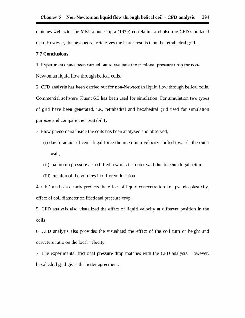
Chapter 7 Non-Newtonian liquid flow through helical coil – CFD analysis 294
matches well with the Mishra and Gupta (1979) correlation and also the CFD simulated
data. However, the hexahedral grid gives the better results than the tetrahedral grid.
7.7 Conclusions
1. Experiments have been carried out to evaluate the frictional pressure drop for non-
Newtonian liquid flow through helical coils.
2. CFD analysis has been carried out for non-Newtonian liquid flow through helical coils.
Commercial software Fluent 6.3 has been used for simulation. For simulation two types
of grid have been generated, i.e., tetrahedral and hexahedral grid used for simulation
purpose and compare their suitability.
3. Flow phenomena inside the coils has been analyzed and observed,
(i) due to action of centrifugal force the maximum velocity shifted towards the outer
wall,
(ii) maximum pressure also shifted towards the outer wall due to centrifugal action,
(iii) creation of the vortices in different location.
4. CFD analysis clearly predicts the effect of liquid concentration i.e., pseudo plasticity,
effect of coil diameter on frictional pressure drop.
5. CFD analysis also visualized the effect of liquid velocity at different position in the
coils.
6. CFD analysis also provides the visualized the effect of the coil turn or height and
curvature ratio on the local velocity.
7. The experimental frictional pressure drop matches with the CFD analysis. However,
hexahedral grid gives the better agreement.

Chapter 7 Non-Newtonian liquid flow through helical coil – CFD analysis 295
E: Solution Tank, HE: Heat Exchanger, LC: Level Controller, P: Pump, P1, P2: PressureTapping, RL1, RL2: Liquid Rotameter, S: Separator, ST: Stirrer, T1, T2: Thermometer,
V1-V11: Valves
Fig. 7.1 Schematic diagram of helical coil
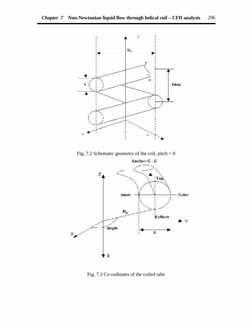
Chapter 7 Non-Newtonian liquid flow through helical coil – CFD analysis 296
Fig. 7.2 Schematic geometry of the coil, pitch = 0
Fig. 7.3 Co-ordinates of the coiled tube

Chapter 7 Non-Newtonian liquid flow through helical coil – CFD analysis 297
Grid Size Level 0, Cells 108263, Faces 237397, Nodes 30060, Partitions1, 1 cell zone, 4face zones
Sectional view
Fig. 7.4 Tetrahedral grid for coilCoil dimension Dt: 0.00933m, Dt/Dc: 0.0529, DC: 0.2662 m, Total length: 5.01m, Turn: 6

Chapter 7 Non-Newtonian liquid flow through helical coil – CFD analysis 298
Grid Size Level 0, Cells 36594, Faces 113106, Nodes 40250, Partitions1, 1 cell zone, 4face zones
Inlet MiddleSectional view
Fig.7.5 Hexahedral grid for coilCoil dimension Dt: 0.00933m, Dt/Dc: 0.0529, DC: 0.2662 m, Total length: 5.01m, Turn: 6

Chapter 7 Non-Newtonian liquid flow through helical coil – CFD analysis 299
(a) (b)
Fig.7.6 Contour plot of static pressure at (a) hexahedral (b) tetrahedral grid,Coil dimension, Dt: 0.00933 m, Dt/Dc: 0.0529, DC: 0.2662 m, Total length: 5.01 m, Turn:
6, Liquid velocity (m/s): 1.7086 and concentration of SCMC solution (kg/m3): 0.8
Fig. 7.7 Contours plot of total pressure at hexahedral grid,Coil dimension, Dt: 0.00933 m, Dt/Dc: 0.0529, DC: 0.2662 m, Total length: 5.01 m, Turn:
6, Liquid velocity (m/s): 1.7086 and concentration of SCMC solution (kg/m3): 0.8
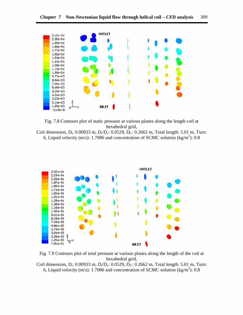
Chapter 7 Non-Newtonian liquid flow through helical coil – CFD analysis 300
Fig. 7.8 Contours plot of static pressure at various planes along the length coil athexahedral grid,
Coil dimension, Dt: 0.00933 m, Dt/Dc: 0.0529, DC: 0.2662 m, Total length: 5.01 m, Turn:6, Liquid velocity (m/s): 1.7086 and concentration of SCMC solution (kg/m3): 0.8
Fig. 7.9 Contours plot of total pressure at various planes along the length of the coil athexahedral grid,
Coil dimension, Dt: 0.00933 m, Dt/Dc: 0.0529, DC: 0.2662 m, Total length: 5.01 m, Turn:6, Liquid velocity (m/s): 1.7086 and concentration of SCMC solution (kg/m3): 0.8

Chapter 7 Non-Newtonian liquid flow through helical coil – CFD analysis 301
300 600 900 1200 1500 2100 2400 2700 3000 3300
Fig. 7.10 Contour plot of static pressure at the different angular plane and at differentturn of the coil
Coil dimension, Dt: 0.00933 m, Dt/Dc: 0.0529, DC: 0.2662 m, Total length: 5.01 m, Turn:6, Liquid velocity (m/s): 1.7086 and concentration of SCMC solution (kg/m3): 0.8

Chapter 7 Non-Newtonian liquid flow through helical coil – CFD analysis 302
300 600 900 1200 1500 2100 2400 2700 3000 3300
Fig. 7.11 Contour plot of total pressure at the different angular plane and at differentturn of a coil at hexahedral grid
Coil dimension, Dt: 0.00933 m, Dt/Dc: 0.0529, DC: 0.2662 m, Total length: 5.01 m, Turn:6, Liquid velocity (m/s): 1.7086 and concentration of SCMC solution (kg/m3): 0.8
Inlet 300 600 900
1200 1500 2400 2700
3000 3300 outletFig. 7.12 Contour plot of static pressure at the different angular plane and at the fixed
turn1 of the coilCoil dimension, Dt: 0.00933 m, Dt/Dc: 0.0529, DC: 0.2662 m, Total length: 5.01 m, Turn:
6, Liquid velocity (m/s): 1.7086 and concentration of SCMC solution (kg/m3): 0.8

Chapter 7 Non-Newtonian liquid flow through helical coil – CFD analysis 303
Inlet 300 600 900
1200 1500 2100 2400
2700 3000 3300 outlet
Fig. 7.13 Contour plot of total pressure at the different angular plane and at the fixedturn1 of the coil
Coil dimension, Dt: 0.00933 m, Dt/Dc: 0.0529, DC: 0.2662 m, Total length: 5.01 m, Turn:6, Liquid velocity (m/s): 1.7086 and concentration of SCMC solution (kg/m3): 0.8
Fig. 7.14 Contour plot of dynamic pressure at hexahedral grid,Coil dimension, Dt: 0.00933 m, Dt/Dc: 0.0529, DC: 0.2662 m, Total length: 5.01 m, Turn:
6, Liquid velocity (m/s): 1.7086 and concentration of SCMC solution (kg/m3): 0.8

Chapter 7 Non-Newtonian liquid flow through helical coil – CFD analysis 304
Fig. 7.15 Contour plot of dynamic pressure at various planes along the length of the coilfor hexahedral grid,
Coil dimension, Dt: 0.00933 m, Dt/Dc: 0.0529, DC: 0.2662 m, Total length: 5.01 m, Turn:6, Liquid velocity (m/s): 1.7086 and concentration of SCMC solution (kg/m3): 0.8
300 600 900 1200 1500 2100 2400 2700 3000 3300
Fig. 7.16 Contour plot of dynamic pressure at the different angular plane and at differentturn or height of the coil at hexahedral grid,
Coil dimension, Dt: 0.00933 m, Dt/Dc: 0.0529, DC: 0.2662 m, Total length: 5.01 m, Turn:6, Liquid velocity (m/s): 1.7086 and concentration of SCMC solution (kg/m3): 0.8

Chapter 7 Non-Newtonian liquid flow through helical coil – CFD analysis 305
300 600 900 1200 1500 2100 2400 2700 3000 3300
Fig. 7.17 Contour plot of dynamic pressure at the different angular plane and at differentturn or height of the coil at hexahedral grid,
Coil dimension, Dt: 0.00933 m, Dt/Dc: 0.0529, DC: 0.2662 m, Total length: 5.01 m, Turn:6, Liquid velocity (m/s): 1.7086 and concentration of SCMC solution (kg/m3): 0.8
Inlet 300 600 900 1200
1500 2100 2400 2700 3000
3300 outletFig. 7.18 Contour plot of dynamic pressure at the different angular plane and at the fixed
turn1 of the coil at hexahedral grid,Coil dimension, Dt: 0.00933 m, Dt/Dc: 0.0529, DC: 0.2662 m, Total length: 5.01m, Turn:
6, Liquid velocity (m/s): 1.7086 and concentration of SCMC solution (kg/m3): 0.8

Chapter 7 Non-Newtonian liquid flow through helical coil – CFD analysis 306
300 600 900 1200
1500 2100 2400 2700
3000 3300
Fig. 7.19 Contour plot of dynamic pressure at the different angular plane and at the fixedturn1 of the coil at hexahedral grid,
Coil dimension, Dt: 0.00933 m, Dt/Dc: 0.0529, DC: 0.2662 m, Total length: 5.01 m, Turn:6, Liquid velocity (m/s): 1.7086 and concentration of SCMC solution (kg/m3): 0.8
Fig. 7.20 Contours plot of velocity magnitude for helical coil at hexahedral grid,Coil dimension, Dt: 0.00933 m, Dt/Dc: 0.0529, DC: 0.2662 m, Total length: 5.01m, Turn:
6, Liquid velocity (m/s): 1.7086 and concentration of SCMC solution (kg/m3): 0.8
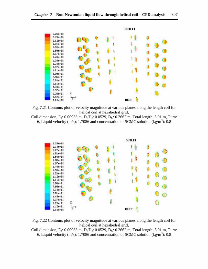
Chapter 7 Non-Newtonian liquid flow through helical coil – CFD analysis 307
Fig. 7.21 Contours plot of velocity magnitude at various planes along the length coil forhelical coil at hexahedral grid,
Coil dimension, Dt: 0.00933 m, Dt/Dc: 0.0529, DC: 0.2662 m, Total length: 5.01 m, Turn:6, Liquid velocity (m/s): 1.7086 and concentration of SCMC solution (kg/m3): 0.8
Fig. 7.22 Contours plot of velocity magnitude at various planes along the length coil forhelical coil at hexahedral grid,
Coil dimension, Dt: 0.00933 m, Dt/Dc: 0.0529, DC: 0.2662 m, Total length: 5.01 m, Turn:6, Liquid velocity (m/s): 1.7086 and concentration of SCMC solution (kg/m3): 0.8
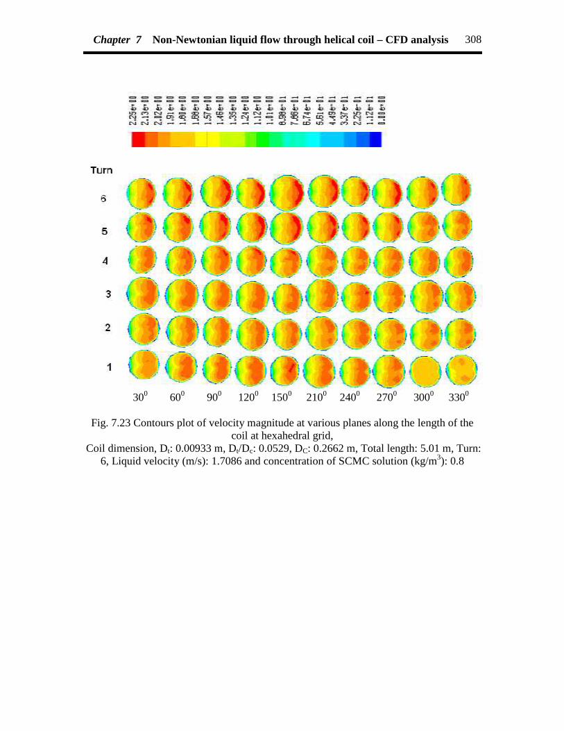
Chapter 7 Non-Newtonian liquid flow through helical coil – CFD analysis 308
300 600 900 1200 1500 2100 2400 2700 3000 3300
Fig. 7.23 Contours plot of velocity magnitude at various planes along the length of thecoil at hexahedral grid,
Coil dimension, Dt: 0.00933 m, Dt/Dc: 0.0529, DC: 0.2662 m, Total length: 5.01 m, Turn:6, Liquid velocity (m/s): 1.7086 and concentration of SCMC solution (kg/m3): 0.8
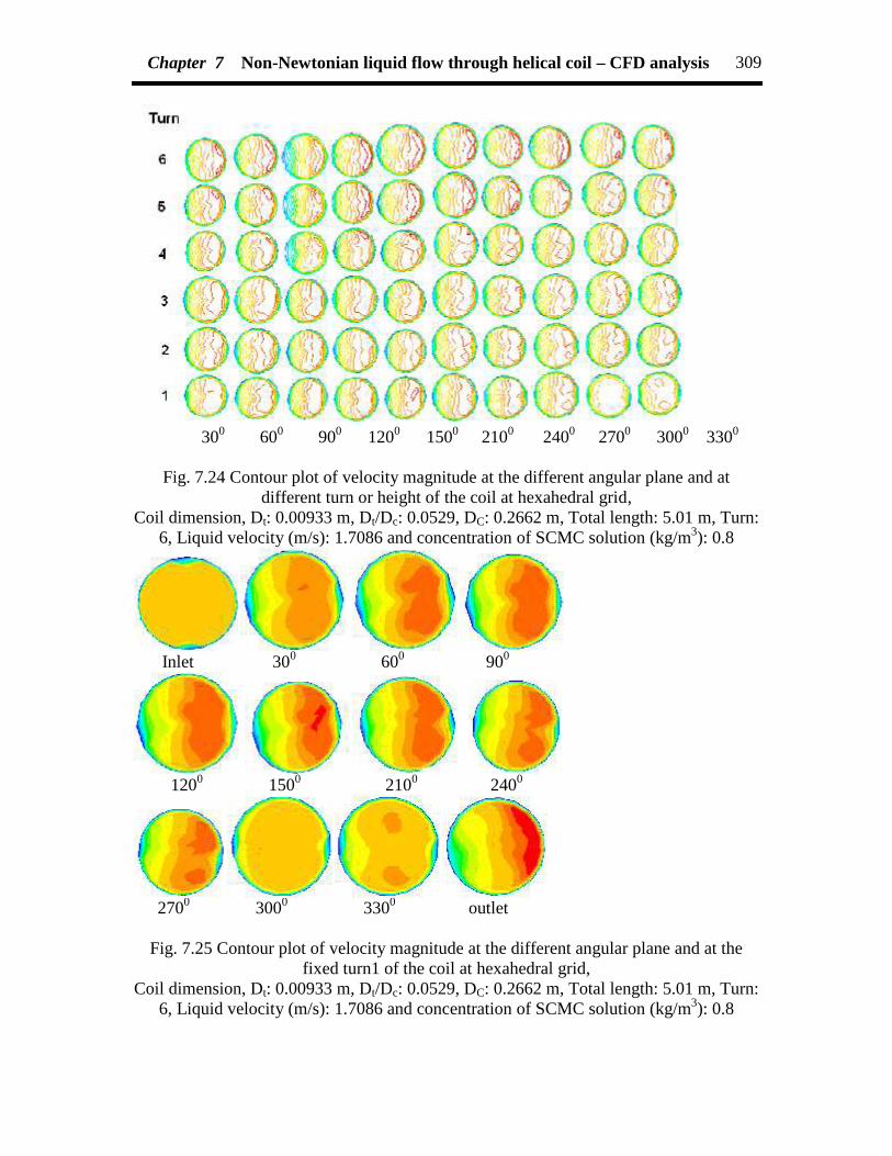
Chapter 7 Non-Newtonian liquid flow through helical coil – CFD analysis 309
300 600 900 1200 1500 2100 2400 2700 3000 3300
Fig. 7.24 Contour plot of velocity magnitude at the different angular plane and atdifferent turn or height of the coil at hexahedral grid,
Coil dimension, Dt: 0.00933 m, Dt/Dc: 0.0529, DC: 0.2662 m, Total length: 5.01 m, Turn:6, Liquid velocity (m/s): 1.7086 and concentration of SCMC solution (kg/m3): 0.8
Inlet 300 600 900
1200 1500 2100 2400
2700 3000 3300 outlet
Fig. 7.25 Contour plot of velocity magnitude at the different angular plane and at thefixed turn1 of the coil at hexahedral grid,
Coil dimension, Dt: 0.00933 m, Dt/Dc: 0.0529, DC: 0.2662 m, Total length: 5.01 m, Turn:6, Liquid velocity (m/s): 1.7086 and concentration of SCMC solution (kg/m3): 0.8

Chapter 7 Non-Newtonian liquid flow through helical coil – CFD analysis 310
300 600 900 1200
1500 2100 2400 2700
3000 3300
Fig. 7.26 Contour plot of velocity magnitude at the different angular plane and at thefixed turn1 of the coil at hexahedral grid,
Coil dimension, Dt: 0.00933 m, Dt/Dc: 0.0529, DC: 0.2662 m, Total length: 5.01 m, Turn:6, Liquid velocity (m/s): 1.7086 and concentration of SCMC solution (kg/m3): 0.8
Fig. 7.27 Contours plot of velocity for helical coil at hexahedral grid, Coil dimension, Dt:0.00933 m, Dt/Dc: 0.0529, DC: 0.2662 m, Total length: 5.01 m, Turn: 6, Liquid velocity
(m/s): 1.7086 and concentration of SCMC solution (kg/m3): 0.8

Chapter 7 Non-Newtonian liquid flow through helical coil – CFD analysis 311
Fig. 7.28 Contours plot of velocity at various planes along the length coil for helical coilat hexahedral grid,
Coil dimension, Dt: 0.00933 m, Dt/Dc: 0.0529, DC: 0.2662 m, Total length: 5.01 m, Turn:6, Liquid velocity (m/s): 1.7086 and concentration of SCMC solution (kg/m3): 0.8
300 600 900 1200 1500 2100 2400 2700 3000 3300
Fig. 7.29 Contour plot of velocity at the different angular plane and at different turn ofthe coil at hexahedral grid,
Coil dimension, Dt: 0.00933 m, Dt/Dc: 0.0529, DC: 0.2662 m, Total length: 5.01 m, Turn:6, Liquid velocity (m/s): 1.7086 and concentration of SCMC solution (kg/m3): 0.8

Chapter 7 Non-Newtonian liquid flow through helical coil – CFD analysis 312
300 600 900 1200 1500 2100 2400 2700 3000 3300
Fig. 7.30 Contour plot of velocity at the different angular plane and at different turn ofthe coil at hexahedral grid,
Coil dimension, Dt: 0.00933 m, Dt/Dc: 0.0529, DC: 0.2662 m, Total length: 5.01 m, Turn:6, Liquid velocity (m/s): 1.7086 and concentration of SCMC solution (kg/m3): 0.8

Chapter 7 Non-Newtonian liquid flow through helical coil – CFD analysis 313
300 600 900 1200
1500 2100 2400 2700
3000 3300
Fig. 7.31 Contour plot of velocity at the different angular plane and at the fixed turn1 ofthe coil at hexahedral grid,
Coil dimension, Dt: 0.00933 m, Dt/Dc: 0.0529, DC: 0.2662 m, Total length: 5.01 m, Turn:6, Liquid velocity (m/s): 1.7086 and concentration of SCMC solution (kg/m3): 0.8

Chapter 7 Non-Newtonian liquid flow through helical coil – CFD analysis 314
300 600 900 1200
1500 2100 2400 2700
3000 3300
Fig. 7.32 Contour plot of velocity at the different angular plane and at the fixed turn1 ofthe coil at hexahedral grid,
Coil dimension, Dt: 0.00933 m, Dt/Dc: 0.0529, DC: 0.2662 m, Total length: 5.01 m, Turn:6, Liquid velocity (m/s): 1.7086 and concentration of SCMC solution (kg/m3): 0.8
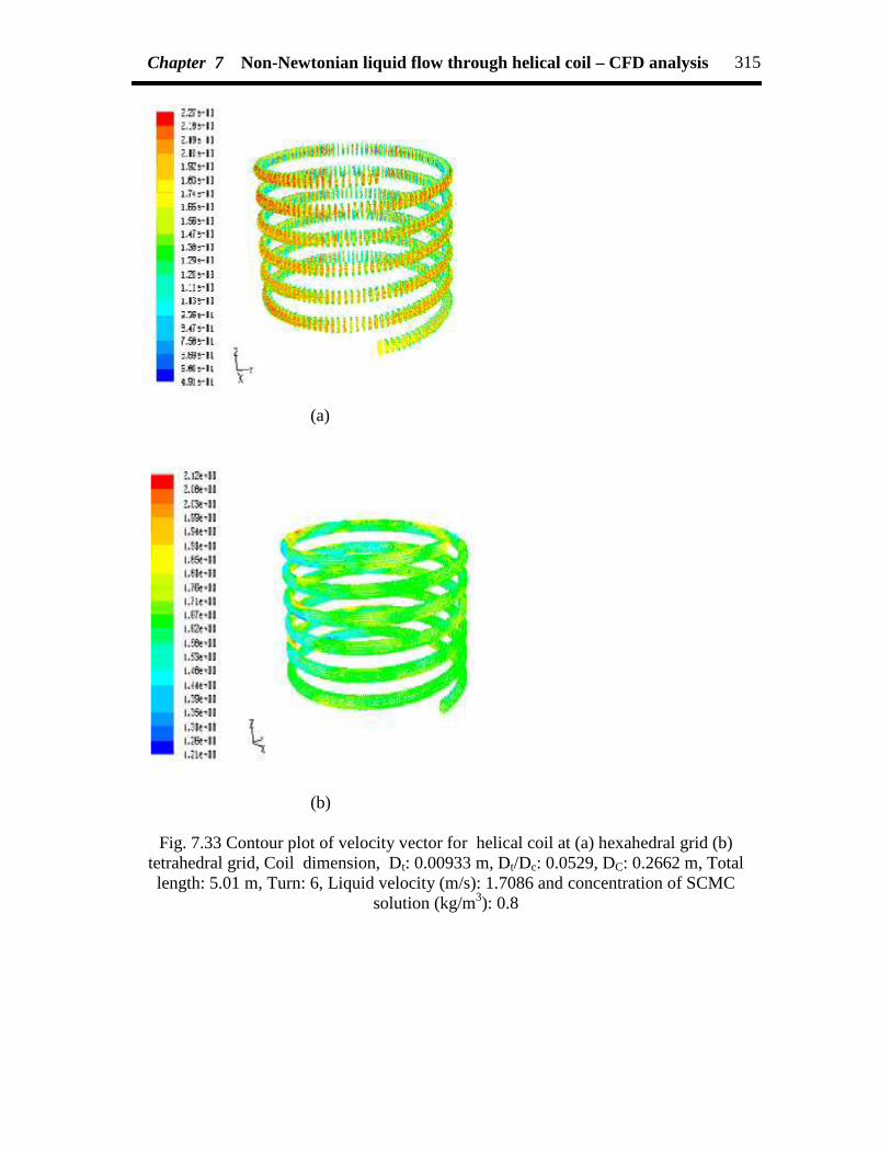
Chapter 7 Non-Newtonian liquid flow through helical coil – CFD analysis 315
(a)
(b)
Fig. 7.33 Contour plot of velocity vector for helical coil at (a) hexahedral grid (b)tetrahedral grid, Coil dimension, Dt: 0.00933 m, Dt/Dc: 0.0529, DC: 0.2662 m, Totallength: 5.01 m, Turn: 6, Liquid velocity (m/s): 1.7086 and concentration of SCMC
solution (kg/m3): 0.8

Chapter 7 Non-Newtonian liquid flow through helical coil – CFD analysis 316
Fig. 7.34 Contour plot of velocity vector at the different angular plane of the coil athexahedral grid,
Coil dimension, Dt: 0.00933 m, Dt/Dc: 0.0529, DC: 0.2662 m, Total length: 5.01 m, Turn:6, Liquid velocity (m/s): 1.7086 and concentration of SCMC solution (kg/m3): 0.8
300 600 900 1200 1500 2100 2400 2700 3000 3300
Fig. 7.35 Contour plot of velocity vector at the different angular plane and at differentturn or height of the coil at hexahedral grid, Coil dimension, Dt: 0.00933 m, Dt/Dc:
0.0529, DC: 0.2662 m, Total length: 5.01 m, Turn: 6, Liquid velocity (m/s): 1.7086 andconcentration of SCMC solution (kg/m3): 0.8

Chapter 7 Non-Newtonian liquid flow through helical coil – CFD analysis 317
Inlet 300 600 900 1200
1500 2100 2400 2700
3000 3300 outlet
Fig. 7.36 Contour plot of velocity vector at the different angular plane and at the fixedturn1 of the coil at hexahedral grid, Coil dimension, Dt: 0.00933 m, Dt/Dc: 0.0529, DC:
0.2662 m, Total length: 5.01 m, Turn: 6, Liquid velocity (m/s): 1.7086 and concentrationof SCMC solution (kg/m3): 0.8

Chapter 7 Non-Newtonian liquid flow through helical coil – CFD analysis 318
Fig. 7.37 Contour plot of helicity for helical coil at hexahedral grid,Coil dimension, Dt: 0.00933 m, Dt/Dc: 0.0529, DC: 0.2662 m, Total length: 5.01 m, Turn:
6, Liquid velocity (m/s): 1.7086 and concentration of SCMC solution (kg/m3): 0.8
Fig. 7.38 Contour plot of vorticity for helical coil at hexahedral grid,Coil dimension, Dt: 0.00933 m, Dt/Dc: 0.0529, DC: 0.2662 m, Total length: 5.01 m, Turn:
6, Liquid velocity (m/s): 1.7086 and concentration of SCMC solution (kg/m3): 0.8

Chapter 7 Non-Newtonian liquid flow through helical coil – CFD analysis 319
Fig. 7.39 Contour plot of cell Reynolds number for helical coil at hexahedral grid,Coil dimension, Dt: 0.00933 m, Dt/Dc: 0.0529, DC: 0.2662 m, Total length: 5.01 m, Turn:
6, Liquid velocity (m/s): 1.7086 and concentration of SCMC solution (kg/m3): 0.8
Fig. 7.40 Contour plot of strain rate at hexahedral grid,Coil dimension, Dt: 0.00933 m, Dt/Dc: 0.0529, DC: 0.2662 m, Total length: 5.01 m, Turn:
6, Liquid velocity (m/s): 1.7086 and concentration of SCMC solution (kg/m3): 0.8
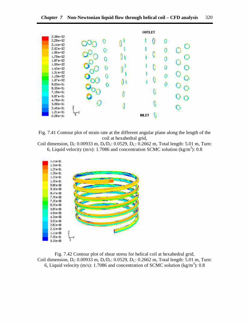
Chapter 7 Non-Newtonian liquid flow through helical coil – CFD analysis 320
Fig. 7.41 Contour plot of strain rate at the different angular plane along the length of thecoil at hexahedral grid,
Coil dimension, Dt: 0.00933 m, Dt/Dc: 0.0529, DC: 0.2662 m, Total length: 5.01 m, Turn:6, Liquid velocity (m/s): 1.7086 and concentration SCMC solution (kg/m3): 0.8
Fig. 7.42 Contour plot of shear stress for helical coil at hexahedral grid,Coil dimension, Dt: 0.00933 m, Dt/Dc: 0.0529, DC: 0.2662 m, Total length: 5.01 m, Turn:
6, Liquid velocity (m/s): 1.7086 and concentration of SCMC solution (kg/m3): 0.8
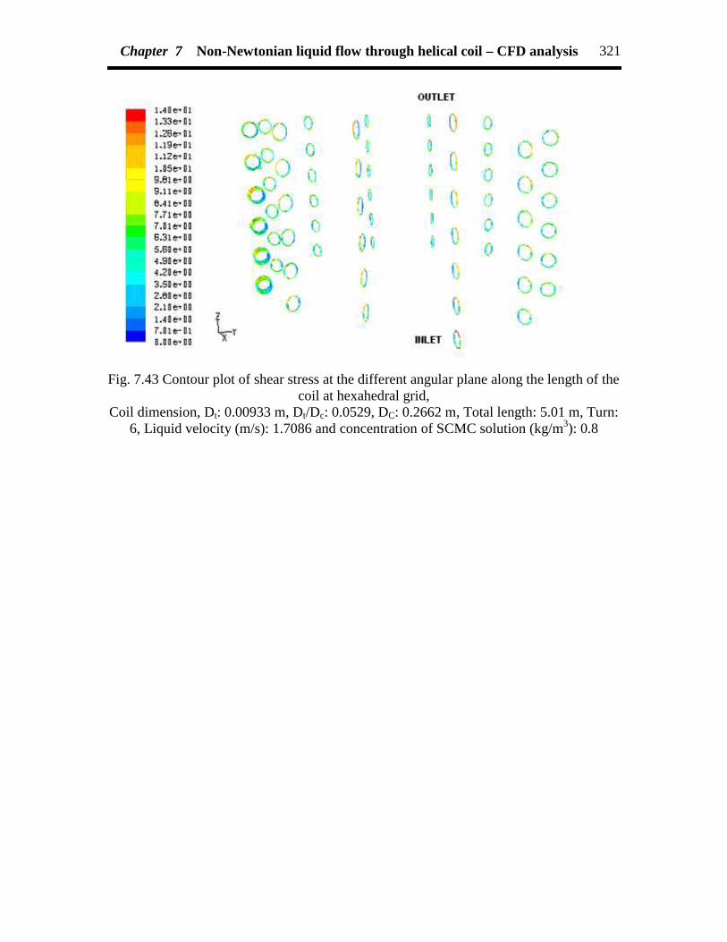
Chapter 7 Non-Newtonian liquid flow through helical coil – CFD analysis 321
Fig. 7.43 Contour plot of shear stress at the different angular plane along the length of thecoil at hexahedral grid,
Coil dimension, Dt: 0.00933 m, Dt/Dc: 0.0529, DC: 0.2662 m, Total length: 5.01 m, Turn:6, Liquid velocity (m/s): 1.7086 and concentration of SCMC solution (kg/m3): 0.8

Chapter 7 Non-Newtonian liquid flow through helical coil – CFD analysis 322
0.4 0.6 0.8 1.0 1.2 1.4 1.6 1.8 2.0
0.0
0.5
1.0
1.5
2.0
2.5
3.0
3.5
4.0
4.5
Sing
le-p
hase
fric
tiona
l pre
ssur
e dr
oppe
r uni
t len
gth
of th
e co
il, k
pa/m
Liquid flow rate, Qlx105, m3/s
Tube diameter(D):0.00933mCoil diameter(D
c): 0.2162m
Symbol Type SCMC Conc., (kg/m3)
Expt. 0.2 CFD,T-grid 0.2 CFD, Hex-bl 0.2 Expt. 0.4 CFD, T-grid 0.4 CFD, Hex-bl 0.4 Expt. 0.6 CFD, T-grid 0.6 CFD, Hex-bl 0.6 Expt. 0.8 CFD, T-grid 0.8 CFD, Hex-bl 0.8
Fig. 7.44 Comparison plot of helical coil at different SCMC concentration
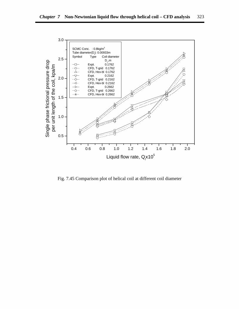
Chapter 7 Non-Newtonian liquid flow through helical coil – CFD analysis 323
0.4 0.6 0.8 1.0 1.2 1.4 1.6 1.8 2.0
0.5
1.0
1.5
2.0
2.5
3.0
Sing
le p
hase
fric
tiona
l pre
ssur
e dr
oppe
r uni
t len
gth
of th
e co
il, k
pa/m
Liquid flow rate, Qlx105
SCMC Conc. : 0.8kg/m3
Tube diameter(Dt): 0.00933mSymbol Type Coil diameter Dc,m
Expt. 0.1762 CFD, T-grid 0.1762 CFD, Hex-bl 0.1762 Expt. 0.2162 CFD, T-grid 0.2162 CFD, Hex-bl 0.2162 Expt. 0.2662 CFD, T-grid 0.2662 CFD, Hex-bl 0.2662
Fig. 7.45 Comparison plot of helical coil at different coil diameter

Chapter 7 Non-Newtonian liquid flow through helical coil – CFD analysis 324
-50 0 50 100 150 200 250 300 3500.8
1.0
1.2
1.4
1.6
1.8
2.0
2.2D
imen
sion
less
she
ar s
tress
Angle (deg)
BL, Hex Grid T-Grid
(a)

Chapter 7 Non-Newtonian liquid flow through helical coil – CFD analysis 325
0 1 2 3 4 50
1
2
3
4
5Pr
edic
ted
pres
sure
dro
p(kp
a)
Measured pressure drop(kpa)
T-grid Hex,bl
(b)
Fig. 7.46 Comparison of present prediction with the experimental data (a) dimensionlessshear stress (b) pressure drop
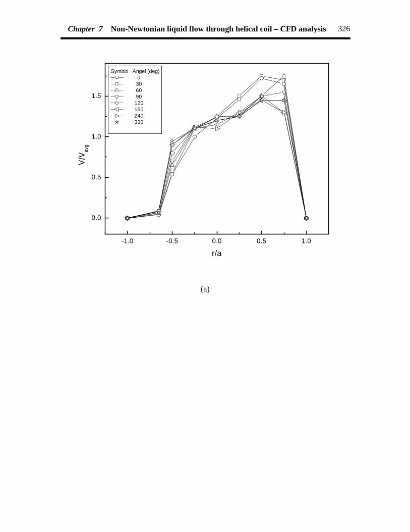
Chapter 7 Non-Newtonian liquid flow through helical coil – CFD analysis 326
-1.0 -0.5 0.0 0.5 1.0
0.0
0.5
1.0
1.5
V/V av
g
r/a
Symbol Angel (deg) 0 30 60 90 120 150 240 330
(a)

Chapter 7 Non-Newtonian liquid flow through helical coil – CFD analysis 327
-1.0 -0.5 0.0 0.5 1.0
0.0
0.5
1.0
1.5V/
V avg
r/a
Symbol Angel(deg) 0 30 60 90 120 150 240 330
(b)
Fig. 7.47 Development of axial velocity profile at different cross-sectional planes incurved tube at curvature ratio = 28, coil turn=2, VL=1.7086 m/s, Liquid (SCMC)concentration (kg/m3) =0.8 in (a) horizontal centerline and (b) vertical centerline

Chapter 7 Non-Newtonian liquid flow through helical coil – CFD analysis 328
-1.0 -0.5 0.0 0.5 1.0
0.0
0.5
1.0
1.5V/
V avg
r/a
VL=0.9765 m/s VL=1.2210 m/s VL=1.4641 m/s VL=1.7086 m/s VL=1.9531 m/s
Fig. 7.48 Effect of liquid velocity on development of axial velocity profile in curved tubeat curvature ratio=28, coil turn = 2

Chapter 7 Non-Newtonian liquid flow through helical coil – CFD analysis 329
-1.0 -0.5 0.0 0.5 1.0
0.0
0.5
1.0
1.5V/
V avg
r/a
H=0.67, Expt. H=0.67, T-grid H=0.67, Hex,bl H=2,Expt. H=2,T-grid H=2,Hex,bl
(a)

Chapter 7 Non-Newtonian liquid flow through helical coil – CFD analysis 330
-1.0 -0.5 0.0 0.5 1.0
0.0
0.5
1.0
V/V av
g
r/a
H=0.67,Expt. H=0.67,T-grid H=0.67,Hex,bl H=2,Expt. H=2,T-grid H=2,Hex,bl
(b)Fig. 7.49 Effect of coil turn or coil length, H on the development of axial velocity profile
in (a) horizontal centerline (b) vertical centerline

Chapter 7 Non-Newtonian liquid flow through helical coil – CFD analysis 331
-1.0 -0.5 0.0 0.5 1.0
0.0
0.5
1.0
1.5V/
V avg
r/a
Radius of curvature=18, Expt. Radius of curvature=18, T-grid Radius of curvature=18, Hex, bl Radius of curvature=28, Expt. Radius of curvature=28, T-grid Radius of curvature=28, Hex, bl
(a)

Chapter 7 Non-Newtonian liquid flow through helical coil – CFD analysis 332
-1.0 -0.5 0.0 0.5 1.0-0.2
0.0
0.2
0.4
0.6
0.8
1.0
1.2
1.4V/
V avg
r/a
Radius of curvature=28, Expt. Radius of curvature=28, T-grid Radius of curvature=28, Hex, bl Radius of curvature=18, Expt. Radius of curvature=18, T-grid Radius of curvature=18, Hex, bl
(b)
Fig. 7.50 Effect of curvature ratio on the development of axial velocity profile in (a)horizontal centerline (b) vertical centerline, VL = 1.7086 m/s, Liquid (SCMC)
concentration (kg/m3) = 0.8

Chapter 7 Non-Newtonian liquid flow through helical coil – CFD analysis 333
0.01 0.10.01
0.1
Cal
cula
ted
f c
Experimental fc
Symbol Type Conc. kg/m3
fc, Mishra & Gupta
0.2 f
c, CFD, Tetrahedral 0.2
fc, CFD, Hexahedral
0.2 f
c, Mishra & Gupta 0.4
fc, CFD, Tetrahedral
0.4 f
c, CFD, Hexahedral 0.4
fc, Mishra & Gupta
0.6 f
c, CFD, Tetrahedral 0.6
fc, CFD, Hexahedral
0.6 f
c, Mishra & Gupta 0.8
fc, CFD, Tetrahedral
0.8 f
c, CFD, Hexahedral 0.8
Fig. 7.51 Comparison plot of the experimental and calculated data for friction factoracross the coil for different liquid (SCMC) concentration
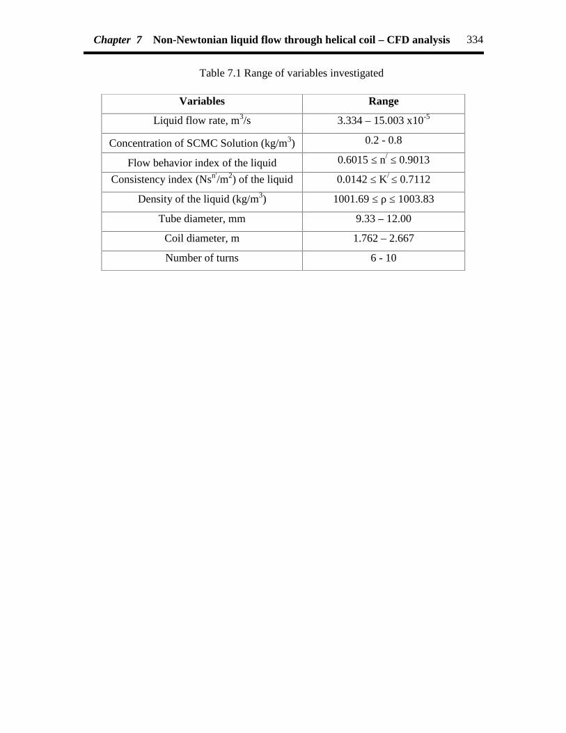
Chapter 7 Non-Newtonian liquid flow through helical coil – CFD analysis 334
Table 7.1 Range of variables investigated
Variables Range
Liquid flow rate, m3/s 3.334 – 15.003 x10⁻⁵
Concentration of SCMC Solution (kg/m3) 0.2 - 0.8
Flow behavior index of the liquid 0.6015 ≤ n/ ≤ 0.9013
Consistency index (Nsn'/m2) of the liquid 0.0142 ≤ K/ ≤ 0.7112
Density of the liquid (kg/m3) 1001.69 ≤ ρ ≤ 1003.83
Tube diameter, mm 9.33 – 12.00
Coil diameter, m 1.762 – 2.667
Number of turns 6 - 10
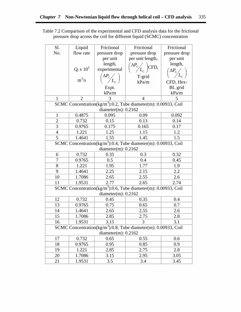
Chapter 7 Non-Newtonian liquid flow through helical coil – CFD analysis 335
Table 7.2 Comparison of the experimental and CFD analysis data for the frictionalpressure drop across the coil for different liquid (SCMC) concentration
Sl.No.
Liquidflow rate
Ql x 105
m3/s
Frictionalpressure drop
per unitlength,
experimental
C
CL
P
Expt.kPa/m
Frictionalpressure drop
per unit length,
C
CL
P CFD,
T-gridkPa/m
Frictionalpressure drop
per unitlength,
C
CL
P
CFD, Hex-BL gridkPa/m
1 2 3 4 5SCMC Concentration(kg/m3):0.2, Tube diameter(m): 0.00933, Coil
diameter(m): 0.21621 0.4875 0.095 0.09 0.0922 0.732 0.15 0.13 0.143 0.9765 0.175 0.165 0.174 1.221 1.25 1.15 1.25 1.4641 1.55 1.45 1.5SCMC Concentration(kg/m3):0.4, Tube diameter(m): 0.00933, Coil
diameter(m): 0.21626 0.732 0.35 0.3 0.327 0.9765 0.5 0.4 0.458 1.221 1.95 1.77 1.99 1.4641 2.25 2.15 2.2
10 1.7086 2.65 2.55 2.611 1.9531 2.77 2.65 2.74SCMC Concentration(kg/m3):0.6, Tube diameter(m): 0.00933, Coil
diameter(m): 0.216212 0.732 0.45 0.35 0.413 0.9765 0.75 0.65 0.714 1.4641 2.65 2.55 2.615 1.7086 2.85 2.75 2.816 1.9531 3.15 3 3.1SCMC Concentration(kg/m3):0.8, Tube diameter(m): 0.00933, Coil
diameter(m): 0.216217 0.732 0.65 0.55 0.618 0.9765 0.95 0.85 0.919 1.221 2.85 2.75 2.820 1.7086 3.15 2.95 3.0521 1.9531 3.5 3.4 3.45

Chapter 7 Non-Newtonian liquid flow through helical coil – CFD analysis 336
Table 7.3 Comparison of the experimental and CFD analysis data for frictional pressuredrop across the coil for liquid (SCMC) concentration of 0.8 kg/m3 and different coil
diameters
Sl.No.
Liquidflow rate
Ql x 105
m3/s
Frictional pressuredrop per unit length,
experimental
C
CL
P Expt.
kPa/m
Frictionalpressure drop
per unit length,
C
CL
P CFD
T-gridkPa/m
Frictionalpressure drop
per unitlength,
C
CL
P
CFDHex-BL grid
kPa/m1 2 3 4 5
Tube diameter(m): 0.00933, Coil diameter(m): 0.1762
1 0.732 0.529 0.45 0.52 0.9765 0.65 0.55 0.63 1.221 0.85 0.75 0.85 1.4641 1.12 1 1.16 1.7086 1.65 1.55 1.67 1.9531 2.25 2.1 2.2
Tube diameter(m): 0.00933, Coil diameter(m): 0.2162
8 0.732 0.8 0.75 0.789 0.9765 0.95 0.88 0.9
10 1.221 1.3 1.2 1.2511 1.7086 1.6 1.45 1.5512 1.9531 1.95 1.85 1.913 0.4875 0.65 0.55 0.6
Tube diameter(m): 0.00933, Coil diameter(m): 0.2662
14 0.732 0.95 0.85 0.915 0.9765 1.33 1.25 1.316 1.221 1.65 1.55 1.617 1.4641 1.95 1.85 1.918 1.7086 2.25 2.15 2.219 1.9531 2.65 2.55 2.6

Chapter 7 Non-Newtonian liquid flow through helical coil – CFD analysis 337
Table 7.4 Comparison of the experimental and calculated data for friction factor acrossthe coil for different liquid (SCMC) concentration
Sl.No.
Liquidflow rate
Ql x 105
m3/s
Reynolds’snumber ofliquid
Rel
Deannumberof liquid
Del
Frictionfactor
fc, Expt.
Frictionfactor
fc, Mishra
& Gupta
Frictionfactor
fc, CFD,
Tetrahedral
Frictionfactor
fc, CFD,
Hexahedral
SCMC Concentration(kg/m3):0.2, Tube diameter(m): 0.00933, Coil diameter(m): 0.26621. 6.67 1247.11 233.47 0.0126 0.0258 0.0256 0.0252. 8.34 1593.60 298.32 0.0222 0.0223 0.0222 0.0223. 10.00 1947.05 0.0082 364.48 0.0198 0.0197 0.019SCMC Concentration(kg/m3):0.4, Tube diameter(m): 0.00933, Coil diameter(m): 0.26621. 6.67 1247.11 233.45 0.0260 0.0260 0.025 0.0222. 8.34 1593.60 298.32 0.0220 0.0223 0.0222 0.0223. 10.00 1947.05 364.48 0.0196 0.0198 0.0197 0.019SCMC Concentration(kg/m3):0.6, Tube diameter(m): 0.00933, Coil diameter(m): 0.26621. 6.67 417.29 78.11 0.0412 0.0411 0.041 0.042. 8.34 552.25 103.38 0.0351 0.0354 0.0353 0.03523. 10.00 694.32 129.97 0.0381 0.0381 0.038 0.0374. 11.67 842.61 157.73 0.0334 0.0334 0.0332 0.0335. 13.34 996.43 186.53 0.0299 0.0300 0.028 0.027SCMC Concentration(kg/m3):0.8, Tube diameter(m): 0.00933, Coil diameter(m): 0.26621. 6.67 187.61 35.12 0.10069 0.10124 0.10123 0.101222. 8.34 256.32 47.08 0.0785 0.0788 0.0787 0.07863. 10.00 330.76 61.91 0.0647 0.0647 0.0646 0.06424. 11.67 410.33 76.81 0.0549 0.0551 0.055 0.0525. 13.34 494.58 92.59 0.0480 0.0482 0.0481 0.048

Chapter 8
Gas-non-Newtonian liquid flow through helical coils – CFDanalysis
Chapter 8 Gas-non-Newtonian liquid ------ helical coils - CFD analysis 339
This chapter deals with the Computational Fluid Dynamics (CFD) analysis to
evaluate the frictional pressure drop for gas-non-Newtonian liquid through helical coils.
The CFD analysis is verified with the experimental data obtained from our earlier
experiments carried out by Biswas (2006) and Biswas & Das (2008).
8.1 Introduction
Two–phase flow through helical coil is much more complex in nature than that of
straight pipes. Due to centrifugal action, when flow enters the curved position the
heavier density phase, i.e., liquid is subjected to a larger centrifugal force which causes
liquid to move away from the centre of curvature while the gas flows towards the centre
of curvature. Despite various applications, the literature on two–phase flow through
coiled tubes in rather scanty. The reasons for the lack of fundamental knowledge on two-
phase flows are three-fold (Mandal and Das, 2003),
i. Two-phase gas-liquid flow is a very complex physical phenomenon where many
types flow regimes can exist (annular flow, jet flow, slug flow, bubbly flow, etc.);
ii. The complex physical laws and mathematical treatment of phenomena occurring
in the presence of the two phases (interface dynamics, coalescence, break-up,
drag, etc.) are still largely undeveloped;
iii. The numeric for solving the governing equations and closure laws of two-phase
flows are extremely complex. Very often two-phase flows show inherent
oscillatory behavior, requiring costly transient solution algorithms.
Owhadi et al. (1968) studied steam-water flow through coils and reported the two-
phase frictional pressure drop agreed well the Lockhart-Martinelli (1949) correlation.
Akagawa et al. (1971) studied gas-liquid flow through helically coiled tubes and

Chapter 8 Gas-non-Newtonian liquid ------ helical coils - CFD analysis 340
observed that the Lockhart-Martinelli (1949) correlation predicted their frictional
pressure drop. Watanabe et al. (1986) studied air-water flow through helical coils and
they experimentally found out the thickness of different points around the circumference.
Unal et al. (1981) reported their experimental investigation on steam-water flow through
coils and observed that the curvature ratio (Dc/d) had the very little influence on the two-
phase pressure drop and proposed empirical correlation for the prediction of the two-
phase pressure drop. Chen and Zhou (1981) tested the steam-water two-phase flow
through vertical helical coils and proposed modified Lockhart-Martinelli (1949)
correlation for their two-phase frictional pressure drop. Hart et al. (1988) studied single
and gas-liquid flow through coils. Saxena et al. (1996) studied air-water flow through
helical coils and observed that close similarities between the flow patterns in coiled tubes
and those of the inclined tubes reported by Spedding et al. (1982). Czop et al. (1994)
carried out experiments on two-phase SF6-water flow through coil and observed that the
Lockhart-Martinelli (1949) correlation gave the better prediction for the two-phase
frictional pressure drop. Guo et al. (1994) studied steam-water flow through horizontal
helical coils at high pressure and proposed empirical correlation for frictional pressure
drop. Awaad et al. (1995) studied air-water flow through coils and observed superficial
velocities of air or water had affect the pressure drop multiplier significantly, where as
helix angle had insignificant effect on two-phase pressure drop. Saxena et al. (1996)
proposed a model that describes the liquid residence time distribution for upward and
downward co-current air-water two-phase flow in coiled tubes for turbulent and laminar
liquid flow. Xin et al. (1997) reported air-water two-phase flow through coils and
proposed a two-phase frictional pressure drop equation by modifying the Lockhart-
Chapter 8 Gas-non-Newtonian liquid ------ helical coils - CFD analysis 341
Martinelli (1949) parameter. They observed that the experimental holdup data matches
well with the Lockhart-Martinelli (1949) correlation. Guo et al. (2001) studied steam-
water two-phase flow through inclined helical coils and compared the two-phase pressure
drop with the horizontal helical coils, and modified Chen’s (1982) correlation to analyze
their data. Gao et al. (2003) numerically simulated stratified oil-water two-phase flow in
a horizontal tube. They proposed a new mechanistic approach to correlate the pressure
drop in coils. Mandal and Das (2003) studied gas-Newtonian liquid flow through helical
coils and proposed empirical correlations for two-phase friction factor and void fraction.
Santini et al. (2008) proposed frictional two-phase pressure drop correlation based on the
energy balance of the two-phase mixture for their experiments on the steam-water flow
through helically coiled steam generator. Biswas and Das (2008) studied gas-non-
Newtonian liquid flow through coils and developed empirical correlations for frictional
pressure drop.
In order to achieve optimum performance, an accurate design technique is
necessary for the prediction of two–phase pressure drop through helical coil tube. This
chapter deals with the computational fluid dynamics technique, FLUENT 6.3, to predict
the pressure drop in helical coil tubes.
8.2 Experimental
The detail experimental set up (Fig. 8.1), techniques and results (Table 8.1) are
taken from published Ph. D. thesis of A. B. Biswas (2006) and their subsequent
publication Biswas and Das (2008).

Chapter 8 Gas-non-Newtonian liquid ------ helical coils - CFD analysis 342
8.3 Mathematical Model
Governing equations and numerical methods are described in chapter 2. Laminar,
non-Newtonian Power Law Eulerian model is used as multiphase model for the CFD
analysis. These basic equations (as discussed in chapter 2) are solved subject to the
following boundary conditions,
(i) The helical coils walls are assumed rigid and a no-slip condition is imposed.
(ii) At the outlet, the velocities are free but the normal and tangential stresses are
constrained to be zero and the gauge pressure is set to zero.
(iii) At the inlet, a uniform velocity profile is used with a time varying forcing
function representive of flow in the left portion of the helical coils.
(iv) Negative gravitational acceleration, -9.8 m/s2 is added. Since flow is against
the gravity.
8.3.1 Computational Fluid Dynamics (CFD) Procedure
Geometries for the helical coils are created in Gambit 6.3 preprocessor. A typical
mesh has about 3x10⁴– 2x10⁵ order unstructured t-grid and unstructured boundary layer
hex-wedge cooper schemes are used. Inlet and outlet are located at each end of the helical
coil. The inlet is used to specify the inlet velocity and outlet is used to specify pressure
outlet. These geometries of the coils are imported into Fluent 6.3 in a Cartesian co-
ordinate system. Fluent 6.3 solved the governing equations in 3-D geometry. Laminar
non-Newtonian Power Law model have been used for simulation. The model solves for
Navier-stokes equation at prescribes velocities. The governing equations are non linear
and several iterations of loop must be performed before a convergent solution is obtained.
The first-order upwind scheme is used in the discretization of set of governing equations,

Chapter 8 Gas-non-Newtonian liquid ------ helical coils - CFD analysis 343
standard interpolation schemes is used for calculating cell-face pressures for using the
Segregated solver in Fluent 6.3. Pressure-velocity coupling refers to the numerical
algorithm which uses a combination of continuity and momentum equations to derive an
equation for pressure (or pressure correction) when using the segregated solver. Simple
algorithm is used.
A general procedure to simulate the two-phase gas-non-Newtonian fluid mixing
in helical coil tubes are based on Gambit 6.3 and Fluent 6.3 software is outlined below,
1. Perform meshing under Gambit 6.3.
Create a computational domain at the flow region,
The grids were generated using boundary layer hexahedral meshes and t-
grid (tetrahedral grid),
Controlling a smooth change in the mesh size by size functions,
Specify boundary and continuum types,
Examine the mesh to ensure that the high skewness is below 0.5 for
hexahedral and below 0.9 for tetrahedral mesh.
2. Import the mesh file to Fluent 6.3 and check the mesh.
3. Define a 3-D, unsteady, implicit, and pressure-based solver.
4. Activate the Eulerian laminar non-Newtonian power law multiphase model.
5. Define a Eulerian laminar model. Slip velocity is added.
6. Enable the SCMC properties with laminar flow conditions using the text
command: define/models/viscous/laminar
Chapter 8 Gas-non-Newtonian liquid ------ helical coils - CFD analysis 344
7. Define the phases by setting SCMC as the primary phase and gas as the secondary
phase, and keeping the default selection of Schiller-Naumann drag model in the
phase interaction panel.
8. Define the operating conditions by turning on gravity and specify the operating
density.
9. Solution control methodology – Under relaxation factors – 0.5 for pressure, 0.3
for momentum, 0.1-0.9 for volume fraction, and default values for the other
parameters. Standard schemes – STANDARD for momentum and volume
fraction, and 1st order upwind for other variables. Pressure-velocity SIMPLE
coupling used;
10. Initialize the solution – velocity;
Enable the plotting of residuals during the calculation, and kept the default
convergence criteria, 1 X 10⁻³ for continuity and 1 X 10⁻⁵ all residuals.
8.3.2 Assumptions for air-SCMC flow through helical coils
The following concepts and assumptions were made:
1. The solution temperature is constant at 300C, i.e., room temperature and each phase
is an isothermal and incompressible fluid;
2. A single pressure is shared by both phases;
3. Momentum and continuity equations are solved for each phase;
4. Our system behaves like a plug and slug flow regimes. But we assumed two-phase
flow as a bubbly flow due to simplicity of calculation in which SCMC is treated as
the primary phase while gas is treated as the secondary phase;

Chapter 8 Gas-non-Newtonian liquid ------ helical coils - CFD analysis 345
5. The secondary phase consists of uniform and unchanging bubbles dispersed in a
continuous phase;
6. The bubbles size is assumed to be small, 0.1mm spherical in size;
7. Two–phase Eulerian laminar non-Newtonian power law model is used;
8. Physical properties are uniform throughout;
9. Different phases move at different velocities (slip velocities);
10. The drag force from liquid phase acting on the gas bubbles is included into the
interphase momentum exchange;
11. There are no external body force and virtual mass force, and the effect of lift force
on the bubbles is negligible.
8.4 Results and discussion
8.4.1 Convergence and grid independency
The convergence criterions were set at 10-5 for all equations except for the
transport equation which residual was set at 10-3. A computational domain L≥200D was
used to ensure fully developed flow results could be obtained for all helical coil tubes. In
general the final results depend upon mesh geometries. Subsequent decrement and
increment in mesh resolution by 50% were applied to evaluate if the employed mesh
resolution was adequate to obtain accurate solutions. It was observed that when the mesh
resolution was decreased by 50% the axial velocity profile was 4-10% of the currently
employed mesh velocity profile for helical coils. As the present mesh resolution was
increased by 50% the axial velocity profile changes 1-5% for helical coils. These results
suggest that the current mesh resolution is sufficient to obtained grid independent
solutions for the proposed model.
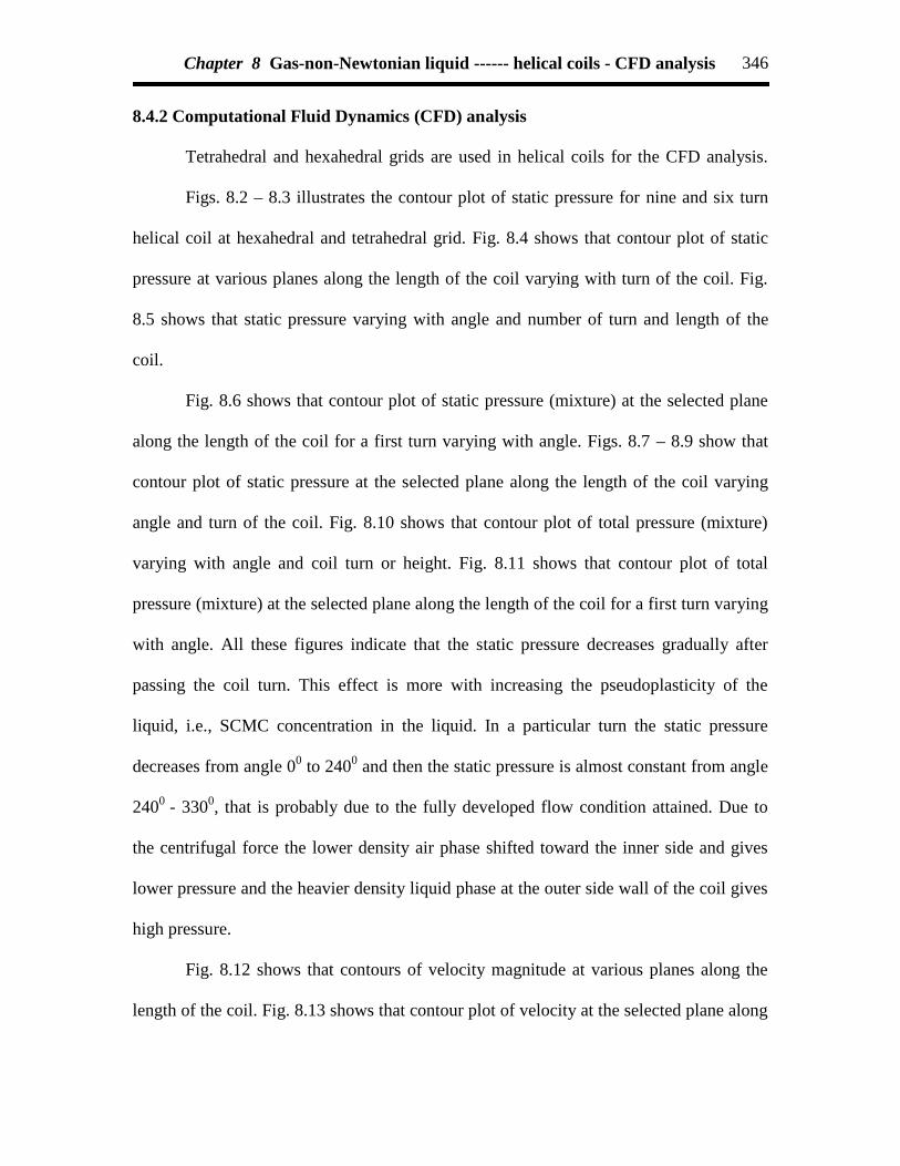
Chapter 8 Gas-non-Newtonian liquid ------ helical coils - CFD analysis 346
8.4.2 Computational Fluid Dynamics (CFD) analysis
Tetrahedral and hexahedral grids are used in helical coils for the CFD analysis.
Figs. 8.2 – 8.3 illustrates the contour plot of static pressure for nine and six turn
helical coil at hexahedral and tetrahedral grid. Fig. 8.4 shows that contour plot of static
pressure at various planes along the length of the coil varying with turn of the coil. Fig.
8.5 shows that static pressure varying with angle and number of turn and length of the
coil.
Fig. 8.6 shows that contour plot of static pressure (mixture) at the selected plane
along the length of the coil for a first turn varying with angle. Figs. 8.7 – 8.9 show that
contour plot of static pressure at the selected plane along the length of the coil varying
angle and turn of the coil. Fig. 8.10 shows that contour plot of total pressure (mixture)
varying with angle and coil turn or height. Fig. 8.11 shows that contour plot of total
pressure (mixture) at the selected plane along the length of the coil for a first turn varying
with angle. All these figures indicate that the static pressure decreases gradually after
passing the coil turn. This effect is more with increasing the pseudoplasticity of the
liquid, i.e., SCMC concentration in the liquid. In a particular turn the static pressure
decreases from angle 00 to 2400 and then the static pressure is almost constant from angle
2400 - 3300, that is probably due to the fully developed flow condition attained. Due to
the centrifugal force the lower density air phase shifted toward the inner side and gives
lower pressure and the heavier density liquid phase at the outer side wall of the coil gives
high pressure.
Fig. 8.12 shows that contours of velocity magnitude at various planes along the
length of the coil. Fig. 8.13 shows that contour plot of velocity at the selected plane along
Chapter 8 Gas-non-Newtonian liquid ------ helical coils - CFD analysis 347
the length of the coil varying with angle and turn of the coil, from 1 – 9. Fig. 8.14
Contour of velocity magnitude at the different angular plane and at any fixed turn of the
coil. Fig. 8.15 shows that contours plot of velocity magnitude for air-phase varying with
angle and coil height and Fig. 8.16 shows that contours of velocity magnitude for air-
phase at the first turn of the coil varying with angle at the selected plane along the length
of the coil. Fig. 8.17 shows that contours plot of velocity magnitude for liquid phase
varying with angle and coil height and Fig. 8.18 shows that contour of velocity
magnitude for liquid phase at the first turn of the coil varying with angle for at the
selected plane along the length of the coil. Fig. 8.19 illustrates the contour plot of velocity
vector coil at hexahedral and tetrahedral grid. Fig. 8.20 shows that plot of velocity vector
varying with angle and coil turn or height at hexahedral grid for helical coil and Fig. 8.21
shows that contours plot of velocity vector at the first turn of the coil varying with angle
for hexahedral grid at the selected plane of the helical coil. Fig. 8.22 shows that contour
plot of velocity vector for liquid phase. Fig. 8.23 shows that velocity vector plot for liquid
phase varying with angle and coil height at hexahedral grid for helical coil. Fig. 8.24
Velocity vector plot for liquid phase varying with angle and coil turn1 at hexahedral grid
at the selected plane of helical coil. Fig. 8.25 shows that contour plot of velocity vector
for air phase at hexahedral grid for helical coil. Fig. 8.26 shows that velocity vector plot
for air phase varying with angle and coil height at hexahedral grid for the helical coil.
Fig. 8.27 shows that contours plot of velocity vector for air phase at the first turn of the
coil varying with angle at hexahedral grid at the selected plane along the length of the
coil.

Chapter 8 Gas-non-Newtonian liquid ------ helical coils - CFD analysis 348
These figures clearly indicates that heavier density goes to outer wall side
of the coil and lower density air phase inner wall side of the coil due to centrifugal force
and their also exists slip between the phases. The velocity changes smoothly to the with
the increase of angle, 00 - 2400, for a particular coil turned and from the angle 2400 - 3300
it is remain unchanged probably due to fully developed flow condition established.
From these plots we observed that air phase shifts the location of the maximum
velocity towards the outer wall of the coiled tube. The velocity profiles flatten when the
velocity is increased until the developing stage is appeared. The developing stage starts
from angle 2400 and end at angle 3300. Since air is lighter, always stating at the inner
upper side of the coil tube.
As fluid flows inside the coil tube a secondary flow develops due to centrifugal
forces. These centrifugal and shear forces move the fluid near the centerline to outer and
the fluid near the walls towards inward direction, resulting a secondary flow known as
Dean vortices. Dean vortices represent centrifugal and shear instabilities that occur when
a viscous fluid flows in a coil tube (Yao and Berger, 1975; Vashisth and Nigam (2009). It
has been shown by Dean (1928b) that a non-dimensional parameter called Dean number
characterizes these flow and defined as,
5.0
Re
d
DDe
c
(8.1)
The Dean number represents the ratio of the square root of the product of the
inertial and centrifugal forces to the viscous force. Since the secondary flows are induced
by the centrifugal force, and their interactions are primarily with the viscous force, the
Dean number is the measure of the magnitude of the secondary flow. Fig. 8.14 clearly

Chapter 8 Gas-non-Newtonian liquid ------ helical coils - CFD analysis 349
characterized by longitudinal vortices and the axial velocity contours show the familiar
C-shape. It also shows the velocity field shifted outer wall of the coil tube.
Fig. 8.28 shows that contour of volume fraction for air-liquid phase varying with
angle and coil turn. Fig. 8.29 shows that volume fraction contours for liquid phase at
various planes along the length of the coil. Fig. 8.30 shows that contours of volume
fraction for liquid phase at the first turn of the coil varying with angle. Fig. 8.31 shows
that contours plot of volume fraction for liquid phase varying with angle and coil height.
Fig. 8.32 shows that contour of volume fraction for air phase at various planes along the
length of the coil. Fig. 8.33 shows that contour plot of volume fraction for air phase at the
first turn of the coil varying with angle. Fig. 8.34 contours plot of volume fraction for air
phase varying with angle and coil height.
All these figures indicate that the volume fraction of the lighter phase, i.e., air, is
gradually covers the top inner side of the coil as the number of turn increases and volume
fraction of the liquid phase is more at the bottom side as turn increase comparing with
the entering condition (Fig. 8.28). But heavier density liquid phase shifted towards the
outer wall and lighter air phase shifted towards the inner wall side with increasing angle
(Fig. 8.30 – 8.33).
Fig. 8.35 shows the liquid path lines in the mixture. It illustrates that heavier
density liquid phase goes to outer wall side of the coil and lighter density air phase goes
to inner side of the coil wall due to centrifugal force and slip existing between the
mixtures.
Fig. 8.36 indicates the two – phase frictional pressure drop per unit length of coil
increases with increasing liquid flow rate at constant SCMC concentration, tube and coil

Chapter 8 Gas-non-Newtonian liquid ------ helical coils - CFD analysis 350
diameter. The experimental results from Biswas and Das (2008) matches well with CFD
simulated result for hexahedral grid than the tetrahedral grid.
Fig. 8.37 indicates the two–phase frictional pressure drop per unit length of coil
increases with increasing the pseudoplasticity of the liquid. The experimental results
Biswas and Das (2008) matches well with CFD simulated results. Fig. 8.38 indicates the
two – phase frictional pressure drop per unit length of coil increases with increasing coil
diameter. The experimental results Biswas and Das (2008) matches well with CFD
simulated results. Fig. 8.39 indicates comparison of present prediction with the
experimental data of Biswas and Das (2008) for the frictional pressure drop and the void
fraction. The predicted data agree well with the experimental data with in an error of ±
15%.
Fig. 8.40 indicates effect of gas and liquid velocity on liquid volume fraction in
curved tube at curvature ratio = 18 and coil length = 2 m. It can be seen from Fig.8.40 at
VL = 0.72 m/s when gas velocity increases from 0.8243 to 1.8243 m/s, the volume
fraction of liquid reduces from 0.51 to 0.38. Fig. 8.41 shows that effect of gas and liquid
velocity on development of axial velocity profile in curved tube at curvature ratio = 18
and coil length = 2 m, VL = 1.9531 m/s, in horizontal centerline. It indicates that velocity
profiles flatten when the liquid velocity is increased.
Fig. 8.42 shows the effect of coil turn or height on the development of axial
velocity profile in (a) horizontal centerline and (b) vertical centerline. It indicates that at
height = 0, the velocity contours are symmetrical to the centerline of the tube. As the coil
turn or height is increased the velocity contours becomes asymmetrical. The axial
velocity profiles for coiled tube at different angular planes are shown in Fig. 8.42(a) for

Chapter 8 Gas-non-Newtonian liquid ------ helical coils - CFD analysis 351
horizontal centerline and Fig. 8.42(b) for vertical centerline. In the horizontal centerline,
the maximum velocity shifts towards the outer wall of the pipe due unbalanced
centrifugal forces on the main flow. It can be seen that the velocity profiles tends to
flatten as the value of coil turn or height decreases for the vertical and horizontal
centerline.
Fig. 8.43 shows that effect of angle on the development of axial velocity profile in
(a) horizontal centerline and (b) vertical centerline. It indicates that the maximum
velocity is shifted towards the outer wall of the coiled tube. It can also state that the flow
gets almost fully developed at angle 2400, since at 2400 and 3300 velocity profiles have
very minor changes. As angle is increased, the axial velocity becomes asymmetrical. Due
to the unbalanced centrifugal forces on the main flow, the maximum velocity shift
towards the outer wall of the coil, in the horizontal centerline.
Fig. 8.44 shows the effect of curvature ratio on the development of axial velocity
profile in (a) horizontal centerline and (b) vertical centerline, at VG = 0.8433 m/s, VL =
1.9531 m/s. It indicates that as the curvature ratio is increased, the coil approaches
towards a straight tube (curvature ratio→∞). This minimizes the curvature effect as
centrifugal forces become less predominant for higher curvature ratio coils. This is
evident from the figure as the velocity profiles flattens in the case of curvature ratio = 18,
due to action of strong centrifugal force.
8.5 Conclusions
1. Computational Fluid Dynamics (CFD) analysis is reported for different gas-non-
Newtonian liquid flow through different coils. The experiments data are taken from
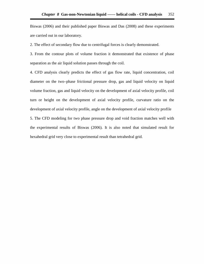
Chapter 8 Gas-non-Newtonian liquid ------ helical coils - CFD analysis 352
Biswas (2006) and their published paper Biswas and Das (2008) and these experiments
are carried out in our laboratory.
2. The effect of secondary flow due to centrifugal forces is clearly demonstrated.
3. From the contour plots of volume fraction it demonstrated that existence of phase
separation as the air liquid solution passes through the coil.
4. CFD analysis clearly predicts the effect of gas flow rate, liquid concentration, coil
diameter on the two–phase frictional pressure drop, gas and liquid velocity on liquid
volume fraction, gas and liquid velocity on the development of axial velocity profile, coil
turn or height on the development of axial velocity profile, curvature ratio on the
development of axial velocity profile, angle on the development of axial velocity profile
5. The CFD modeling for two phase pressure drop and void fraction matches well with
the experimental results of Biswas (2006). It is also noted that simulated result for
hexahedral grid very close to experimental result than tetrahedral grid.

Chapter 8 Gas-non-Newtonian liquid ------ helical coils - CFD analysis 353
A: Compressor, B: Oil Tray, C: Gas Cylinder, D: Gas Regulator, E: Solution Tank, HE:Heat Exchanger, LC: Level Controller, P: Pump, P1, P2: Pressure Tapping, RL1, RL2:
Liquid Rotameter, RG1, RG2: Gas Rotameter, S: Separator, ST: Stirrer, T: T-Mixer, T1,T2: Thermometer, V1-V11: Valves
Fig. 8.1 Schematic diagram of helical coil
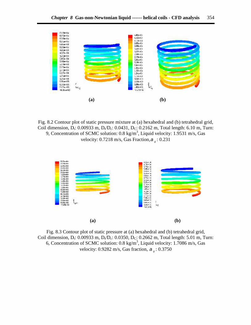
Chapter 8 Gas-non-Newtonian liquid ------ helical coils - CFD analysis 354
(a) (b)
Fig. 8.2 Contour plot of static pressure mixture at (a) hexahedral and (b) tetrahedral grid,Coil dimension, Dt: 0.00933 m, Dt/Dc: 0.0431, DC: 0.2162 m, Total length: 6.10 m, Turn:
9, Concentration of SCMC solution: 0.8 kg/m3, Liquid velocity: 1.9531 m/s, Gasvelocity: 0.7218 m/s, Gas Fraction, g : 0.231
(a) (b)
Fig. 8.3 Contour plot of static pressure at (a) hexahedral and (b) tetrahedral grid,Coil dimension, Dt: 0.00933 m, Dt/Dc: 0.0350, DC: 0.2662 m, Total length: 5.01 m, Turn:
6, Concentration of SCMC solution: 0.8 kg/m3, Liquid velocity: 1.7086 m/s, Gasvelocity: 0.9282 m/s, Gas fraction, g : 0.3750

Chapter 8 Gas-non-Newtonian liquid ------ helical coils - CFD analysis 355
Fig. 8.4 Contour plot of static pressure mixture at various planes along the length of thecoil at hexahedral grid,
Coil dimension, Dt: 0.00933 m, Dt/Dc: 0.0431, DC: 0.2162 m, Total length: 6.10 m, Turn:9, Concentration of SCMC solution: 0.8 kg/m3, Liquid velocity: 1.9531 m/s, Gas
velocity: 0.7218 m/s, Gas Fraction, g : 0.231
Angle (deg) 300 600 900 1200
Fig. 8.5 Contour plot of static pressure, mixture at hexahedral boundary layer gridvarying with coil turn, coil length and angle of the coil,
Coil dimension, Dt: 0.00933 m, Dt/Dc: 0.0431, DC: 0.2162 m, Total length: 6.10 m, Turn:9, Concentration of SCMC solution (kg/m3): 0.8, Liquid velocity, VL (m/s): 1.9531, Gas
velocity, Vg (m/s: 0.7218, Gas Fraction, g :0.2310

Chapter 8 Gas-non-Newtonian liquid ------ helical coils - CFD analysis 356
Fig. 8.6 Contour plot of static pressure (mixture) varying with angle at the first turn of thecoil,
Coil dimension, Dt: 0.00933 m, Dt/Dc: 0.0431, DC: 0.2162 m, Total length: 6.10 m, Turn:9, Concentration of SCMC solution (kg/m3): 0.8, Liquid velocity, VL (m/s): 1.9531, Gas
velocity, Vg (m/s):0.7218, Gas Fraction, g :0.2310

Chapter 8 Gas-non-Newtonian liquid ------ helical coils - CFD analysis 357
Inlet Angle: 00
Turn: 1 2 3 4 5 6 7 8 9Angle: 300
Turn: 1 2 3 4 5 6 7 8 9Angle: 600
Turn: 1 2 3 4 5 6 7 8 9Angle: 900
Turn: 1 2 3 4 5 6 7 8 9Angle: 1200
Turn: 1 2 3 4 5 6 7 8 9Angle: 1500
Turn: 1 2 3 4 5 6 7 8 9
Angle: 2400
Turn: 1 2 3 4 5 6 7 8 9
Angle: 3300
Turn: 1 2 3 4 5 6 7 8 9Fig. 8.7 Contour plot of static pressure at the selected plane along the length of the coil varying
angle and turn of the coil, from 1-9,Coil dimension, Dt: 0.00933 m, Dt/Dc: 0.0431, DC: 0.2162 m, Total length: 6.10 m, Turn: 9,
Concentration of SCMC solution (kg/m3): 0.8, Liquid velocity, VL (m/s): 1.9531, Gas velocity, Vg
(m/s):0.7218, Gas Fraction, g :0.2310

Chapter 8 Gas-non-Newtonian liquid ------ helical coils - CFD analysis 358
Fig. 8.8 Contour plot of static pressure varying with angle and number of turn of the coil,Coil dimension, Tube diameter (m): 0.00933, Dt/Dc: 0.0431, DC: 0.2162 m, Total length:
6.10 m, Turn: 9Concentration of SCMC solution (kg/m3): 0.8, Liquid velocity (m/s): 1.037, Gas velocity
(m/s): 1.9531, Gas fraction, g : 0.2310 Turn: 9

Chapter 8 Gas-non-Newtonian liquid ------ helical coils - CFD analysis 359
Turn: 1Angle: Inlet 00 300 600 900 1200 1500 2400 3300
Turn: 2, Angle: 00 300 600 900 1200 1500 2400 3300
Turn: 3, Angle: 00 300 600 900 1200 1500 2400 3300
Turn: 4, Angle: 00 300 600 900 1200 1500 2400 3300
Turn: 5, Angle: 00 300 600 900 1200 1500 2400 3300
Turn: 6, Angle: 00 300 600 900 1200 1500 2400 3300
Turn: 7, Angle: 00 300 600 900 1200 1500 2400 3300
Turn: 8, Angle: 00 300 600 900 1200 1500 2400 3300
Fig. 8.9 Contour plot of static pressure at different angle and fixed turn of the coil, from1-8 at the selected plane along the length of the coil,
Coil dimension, Tube diameter (m): 0.00933, Dt/Dc: 0.0431, DC: 0.2162 m, Total length:6.10 m, Turn: 9, Concentration of SCMC solution (kg/m3): 0.8, Liquid flow rate (m3/s):
13.34x10⁻⁵, Gas flowrate (m3/s): 4.93x10⁻⁵, Gas fraction, g : 0.2310
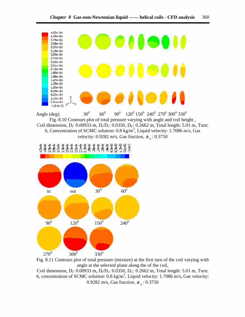
Chapter 8 Gas-non-Newtonian liquid ------ helical coils - CFD analysis 360
Angle (deg): 300 600 900 1200 1500 2400 2700 3000 3300
Fig. 8.10 Contours plot of total pressure varying with angle and coil height ,Coil dimension, Dt: 0.00933 m, Dt/Dc: 0.0350, DC: 0.2662 m, Total length: 5.01 m, Turn:
6, Concentration of SCMC solution: 0.8 kg/m3, Liquid velocity: 1.7086 m/s, Gasvelocity: 0.9282 m/s, Gas fraction, g : 0.3750
in out 300 600
900 1200 1500 2400
2700 3000 3300
Fig. 8.11 Contours plot of total pressure (mixture) at the first turn of the coil varying withangle at the selected plane along the of the coil,
Coil dimension, Dt: 0.00933 m, Dt/Dc: 0.0350, DC: 0.2662 m, Total length: 5.01 m, Turn:6, concentration of SCMC solution: 0.8 kg/m3, Liquid velocity: 1.7086 m/s, Gas velocity:
0.9282 m/s, Gas fraction, g : 0.3750

Chapter 8 Gas-non-Newtonian liquid ------ helical coils - CFD analysis 361
(a)
(b)Fig. 8.12 (a) Contours plot of velocity magnitude for mixture and (b) Contours plot of
velocity magnitudeat various planes along the length of the coil
at hexahedral grid,Coil dimension, Dt: 0.00933 m, Dt/Dc: 0.0431, DC: 0.2162 m, Total length: 6.10 m, Turn:
9, Concentration of SCMC solution: 0.8 kg/m3, Liquid velocity: 1.9531 m/s, Gasvelocity: 0.7218 m/s, Gas fraction, g : 0.231

Chapter 8 Gas-non-Newtonian liquid ------ helical coils - CFD analysis 362
Inlet velocity Outlet velocity
SCMC AIR SCMC AIR
Angle: 00,Turn: 1 2 3 4 5 6 7 8 9
Angle: 300,Turn: 1 2 3 4 5 6 7 8 9
Angle: 600,Turn: 1 2 3 4 5 6 7 8 9
Angle: 900,Turn: 1 2 3 4 5 6 7 8 9
Angle: 1200
Turn: 1 2 3 4 5 6 7 8 9
Angle: 1500
Turn: 1 2 3 4 5 6 7 8 9
Angle: 2400
Turn: 1 2 3 4 5 6 7 8 9Fig. 8.13 Contour plot of velocity at the selected plane along the length of the coil
varying with angle and turn of the coil from 1-9,Coil dimension: Dt: 0.00933 m, Dt/Dc: 0.0431, DC: 0.2162 m, Total length: 6.10 m, Turn:9, concentration of SCMC solution: 0.8kg/m3, Liquid velocity: 1.9531 m/s, Gas velocity:
0.7218 m/s, Gas fraction, g : 0.231
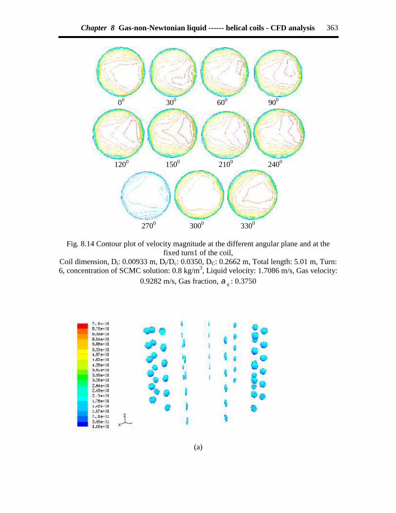
Chapter 8 Gas-non-Newtonian liquid ------ helical coils - CFD analysis 363
00 300 600 900
1200 1500 2100 2400
2700 3000 3300
Fig. 8.14 Contour plot of velocity magnitude at the different angular plane and at thefixed turn1 of the coil,
Coil dimension, Dt: 0.00933 m, Dt/Dc: 0.0350, DC: 0.2662 m, Total length: 5.01 m, Turn:6, concentration of SCMC solution: 0.8 kg/m3, Liquid velocity: 1.7086 m/s, Gas velocity:
0.9282 m/s, Gas fraction, g : 0.3750
(a)

Chapter 8 Gas-non-Newtonian liquid ------ helical coils - CFD analysis 364
Angle (deg): 300 600 1200 1500 2400 2700 3000 3300
(b)Fig. 8.15 (a) Contour plot of velocity magnitude for air phase at various planes along the
length of the coil (b) Contours plot of velocity magnitude for air phase varying with angleand coil height
Coil dimension, Dt: 0.00933 m, Dt/Dc: 0.0350, DC: 0.2662 m, Total length: 5.01 m, Turn:6, concentration of SCMC solution: 0.8 kg/m3, Liquid velocity: 1.7086 m/s, Gas velocity:
0.9282 m/s, Gas fraction, g : 0.3750
in out 300 600 900 1200
1500 2400 2700 3000 3300
Fig. 8.16 Contours plot of velocity magnitude for air phase at the first turn of the coilvarying with angle for hexahedral grid at the selected plane along the length of the coil,
Coil dimension, Dt: 0.00933 m, Dt/Dc: 0.0350, DC: 0.2662 m, Total length: 5.01 m, Turn:6, concentration of SCMC solution: 0.8 kg/m3, Liquid velocity: 1.7086 m/s, Gas velocity:
0.9282 m/s, Gas fraction, g : 0.3750

Chapter 8 Gas-non-Newtonian liquid ------ helical coils - CFD analysis 365
(a)
Angle (deg): 300 600 1200 1500 2400 2700 3000 3300
(b)
Fig. 8.17 (a) Contour plot of velocity magnitude for liquid phase at various planes alongthe length of the coil
(b) Contours plot of velocity magnitude for liquid phase varying with angle and coilheight
at hexahedral grid,Coil dimension, Dt: 0.00933 m, Dt/Dc: 0.0350, DC: 0.2662 m, Total length: 5.01 m, Turn:6, concentration of SCMC solution: 0.8 kg/m3, Liquid velocity: 1.7086 m/s, Gas velocity:
0.9282 m/s, Gas fraction, g : 0.3750

Chapter 8 Gas-non-Newtonian liquid ------ helical coils - CFD analysis 366
inlet outlet 300 600 900 1200
1500 2400 2700 3000 3300
Fig. 8.18 Contours plot of velocity magnitude for liquid phase at the first turn of the coilvarying with angle for hexahedral grid at the selected plane along the length of the coil,
Coil dimension, Dt: 0.00933 m, Dt/Dc: 0.0350, DC: 0.2662 m, Total length: 5.01 m, Turn:6, concentration of SCMC solution: 0.8 kg/m3, Liquid velocity: 1.7086 m/s, Gas velocity:
0.9282 m/s, Gas fraction, g : 0.3750
(a) (b)
Fig. 8.19 Contour plot of velocity vector at (a) hexahedral and (b) tetrahedral grid,Coil dimension, Dt: 0.00933 m, Dt/Dc: 0.0431, DC: 0.2162 m, Total length: 6.10 m, Turn:9, concentration of SCMC solution: 0.8 kg/m3, Liquid velocity: 1.9531 m/s, Gas velocity:
0.7218 m/s, Gas fraction, g : 0.231
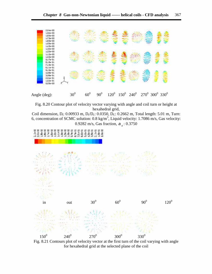
Chapter 8 Gas-non-Newtonian liquid ------ helical coils - CFD analysis 367
Angle (deg): 300 600 900 1200 1500 2400 2700 3000 3300
Fig. 8.20 Contour plot of velocity vector varying with angle and coil turn or height athexahedral grid,
Coil dimension, Dt: 0.00933 m, Dt/Dc: 0.0350, DC: 0.2662 m, Total length: 5.01 m, Turn:6, concentration of SCMC solution: 0.8 kg/m3, Liquid velocity: 1.7086 m/s, Gas velocity:
0.9282 m/s, Gas fraction, g : 0.3750
in out 300 600 900 1200
1500 2400 2700 3000 3300
Fig. 8.21 Contours plot of velocity vector at the first turn of the coil varying with anglefor hexahedral grid at the selected plane of the coil

Chapter 8 Gas-non-Newtonian liquid ------ helical coils - CFD analysis 368
Coil dimension, Dt: 0.00933 m, Dt/Dc: 0.0350, DC: 0.2662 m, Total length: 5.01 m, Turn:6, Concentration of SCMC solution : 0.8kg/m3, Liquid velocity: 1.7086 m/s, Gas
velocity: 0.9282 m/s, Gas fraction, g : 0.3750
(a) Velocity vector plot for liquid phase
(b) Velocity vector plot for liquid phase at various planes along the length of the coil
Fig. 8.22 Contour plot of velocity vector for liquid phase at hexahedral grid,Coil dimension, Dt: 0.00933 m, Dt/Dc: 0.0529, DC: 0.2662 m, Total length: 5.01 m, Turn:
6, Concentration of SCMC solution: 0.8 kg/m3, Liquid velocity: 1.7086 m/s, Gasvelocity: 0.9282 m/s, Gas fraction, g : 0.3750

Chapter 8 Gas-non-Newtonian liquid ------ helical coils - CFD analysis 369
Angle (deg): 300 600 900 1200 1500 2400 2700 3000 3300
Fig. 8.23 Contour plot of velocity vector for liquid phase varying with angle and coilheight at hexahedral grid,
Coil dimension, Dt: 0.00933 m, Dt/Dc: 0.0350, DC: 0.2662 m, Total length: 5.01 m, Turn:6, Concentration of SCMC solution: 0.8 kg/m3, Liquid velocity: 1.7086 m/s, Gas
velocity: 0.9282 m/s, Gas fraction, g : 0.3750
in out 300 600 900 1200
1500 2400 2700 3000 3300

Chapter 8 Gas-non-Newtonian liquid ------ helical coils - CFD analysis 370
Fig. 8.24 Contour plot of velocity vector plot for liquid phase varying with angle and coilturn1 at hexahedral grid at the selected plane of the coil,
Coil dimension, Dt: 0.00933 m, Dt/Dc: 0.0350, DC: 0.2662 m, Total length: 5.01 m, Turn:6, Concentration of SCMC solution: 0.8 kg/m3, Liquid velocity: 1.7086 m/s, Gas
velocity: 0.9282 m/s, Gas fraction, g : 0.3750
(a)
(b)
Fig. 8.25 (a) Contour plot of velocity vector for air phase and (b) velocity vector plot forair phase at various plane along the length of the coil at hexahedral grid,
Coil dimension, Dt: 0.00933 m, Dt/Dc: 0.0529, DC: 0.2662 m, Total length: 5.01 m, Turn:6, Concentration of SCMC solution: 0.8 kg/m3, Liquid velocity: 1.7086 m/s, Gas
velocity: 0.9282 m/s, Gas fraction, g : 0.3750

Chapter 8 Gas-non-Newtonian liquid ------ helical coils - CFD analysis 371
Angle (deg): 300 600 900 1200 1500 2400 2700 3000 3300
Fig. 8.26 Contour plot of velocity vector plot for air phase varying with angle and coilheight at hexahedral grid,
Coil dimension, Dt: 0.00933 m, Dt/Dc: 0.0350, DC: 0.2662 m, Total length: 5.01 m, Turn:6, Concentration of SCMC solution: 0.8 kg/m3, Liquid velocity: 1.7086 m/s, Gas
velocity: 0.9282 m/s, Gas fraction: 0.3750
in out 300 600 900 1200
1500 2400 2700 3000 3300
Fig. 8.27 Contours plot of velocity vector for air phase at the first turn of the coil varyingwith angle at hexahedral grid at the selected plane along the length of the coil, Coil

Chapter 8 Gas-non-Newtonian liquid ------ helical coils - CFD analysis 372
dimension, Dt: 0.00933 m, Dt/Dc: 0.0350, DC: 0.2662 m, Total length: 5.01 m, Turn: 6,Concentration of SCMC solution: 0.8 kg/m3, Liquid velocity: 1.7086 m/s, Gas velocity:
0.9282 m/s, Gas fraction, g : 0.3750
Angle (deg) 300 600 900 1200
Phase Air SCMC Air SCMC Air SCMC Air SCMC
Fig. 8.28 Contour plot of volume fraction at the selected plane for air-SCMC phasevarying with angle and coil turn at hexahedral boundary layer grid,
Coil dimension, Dt: 0.00933 m, Dt/Dc: 0.0431, DC: 0.2162 m, Total length: 6.10 m, Turn:9, Concentration of SCMC solution (kg/m3): 0.8, Liquid velocity, VL (m/s): 1.9531, Gas
velocity, Vg (m/s) :0.7218, Gas Fraction, g :0.2310
(a)

Chapter 8 Gas-non-Newtonian liquid ------ helical coils - CFD analysis 373
(b)Fig. 8.29 (a) Contours plot of volume fraction for liquid phase and (b) Contour of
volume fraction for liquid phase at various planes along the length of the coilat hexahedral grid at the selected plane along the length of the coil,
Coil dimension, Dt: 0.00933 m, Dt/Dc: 0.0350, DC: 0.2662 m, Total length: 5.01 m, Turn:6, Concentration of SCMC solution: 0.8 kg/m3, Liquid velocity: 1.7086 m/s, Gas
velocity: 0.9282 m/s, Gas fraction, g : 0.3750

Chapter 8 Gas-non-Newtonian liquid ------ helical coils - CFD analysis 374
in out 300 600 900 1200
1500 2400 2700 3000 3300
Fig. 8.30 Contours plot of volume fraction for liquid phase at the first turn of the coilvarying with angle at hexahedral grid at the selected plane along the length of the coil,
Coil dimension, Dt: 0.00933 m, Dt/Dc: 0.0350, DC: 0.2662 m, Total length: 5.01 m, Turn:6, Concentration of SCMC solution: 0.8 kg/m3, Liquid velocity: 1.7086 m/s, Gas
velocity: 0.9282 m/s, Gas fraction, g : 0.3750
Angle (deg): 300 600 900 1200 1500 2400 2700 3000 3300
Fig. 8.31 Contours plot of volume fraction for liquid phase varying with angle and coilheight
at hexahedral grid,Coil dimension, Dt: 0.00933 m, Dt/Dc: 0.0350, DC: 0.2662 m, Total length: 5.01 m, Turn:
6, Concentration of SCMC solution: 0.8 kg/m3, Liquid velocity: 1.7086 m/s, Gasvelocity: 0.9282 m/s, Gas fraction, g : 0.3750
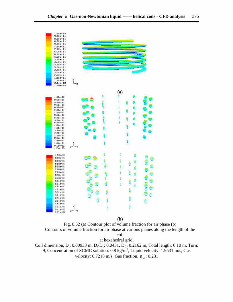
Chapter 8 Gas-non-Newtonian liquid ------ helical coils - CFD analysis 375
(a)
(b)Fig. 8.32 (a) Contour plot of volume fraction for air phase (b)
Contours of volume fraction for air phase at various planes along the length of thecoil
at hexahedral grid,Coil dimension, Dt: 0.00933 m, Dt/Dc: 0.0431, DC: 0.2162 m, Total length: 6.10 m, Turn:
9, Concentration of SCMC solution: 0.8 kg/m3, Liquid velocity: 1.9531 m/s, Gasvelocity: 0.7218 m/s, Gas fraction, g : 0.231

Chapter 8 Gas-non-Newtonian liquid ------ helical coils - CFD analysis 376
in out 300 600 900 1200
1500 2400 2700 3000 3300
Fig. 8.33 Contour plot of volume fraction for air phase at the first turn of the coil varyingwith angle at hexahedral grid at the selected plane along the length of the coil,
Coil dimension, Dt: 0.00933 m, Dt/Dc: 0.0529, DC: 0.2662 m, Total length: 5.01 m, Turn:6, Concentration of SCMC solution: 0.8 kg/m3, Liquid velocity: 1.7086 m/s, Gas
velocity: 0.9282 m/s, Gas fraction, g : 0.3520
Angle (deg): 300 600 900 1200 1500 2400 2700 3000 3300
Fig. 8.34 Contours plot of volume fraction for air phase varying with angle and coilheight ,
Coil dimension, Dt: 0.00933 m, Dt/Dc: 0.0350, DC: 0.2662 m, Total length: 5.01 m, Turn:6, Concentration of SCMC solution: 0.8 kg/m3, Liquid velocity: 1.7086 m/s, Gas
velocity: 0.9282 m/s, Gas fraction, g : 0.3750

Chapter 8 Gas-non-Newtonian liquid ------ helical coils - CFD analysis 377
Fig. 8.35 Path lines of liquid in the mixture
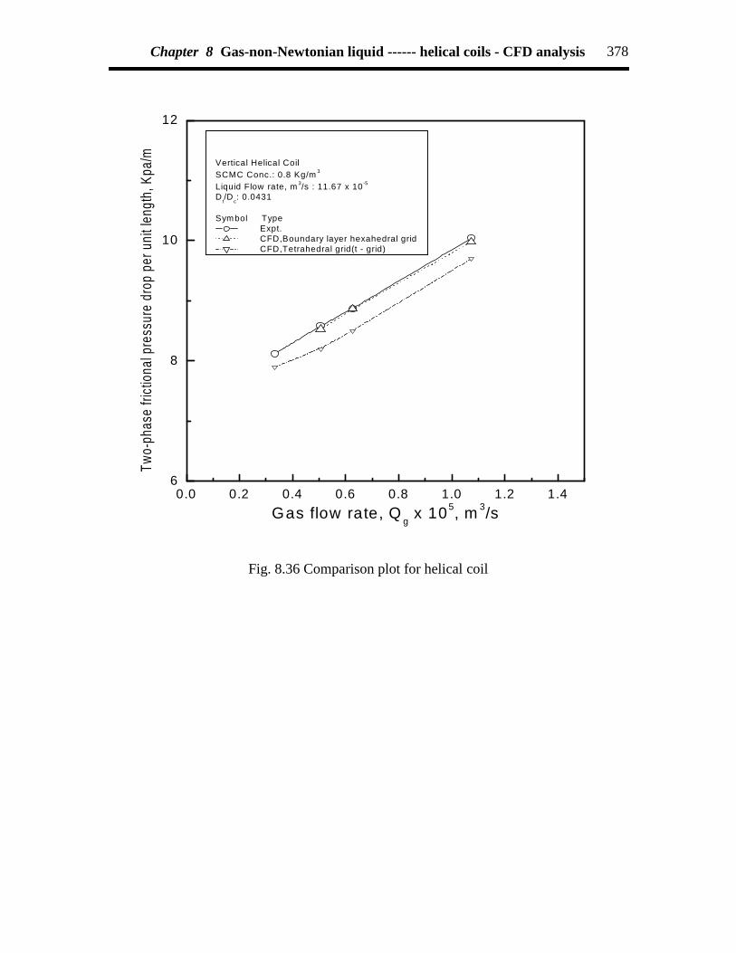
Chapter 8 Gas-non-Newtonian liquid ------ helical coils - CFD analysis 378
0.0 0.2 0.4 0.6 0.8 1.0 1.2 1.46
8
10
12
Two-
phas
e fri
ction
al pr
essu
re d
rop
per u
nit le
ngth
, Kpa
/m
Gas flow rate, Q g x 105, m 3/s
Vertical Helical CoilSCMC Conc.: 0.8 Kg/m 3
Liquid Flow rate, m 3/s : 11.67 x 10 -5
Dt/D
c: 0.0431
Symbol Type Expt. CFD,Boundary layer hexahedral grid CFD,Tetrahedral grid(t - grid)
Fig. 8.36 Comparison plot for helical coil

Chapter 8 Gas-non-Newtonian liquid ------ helical coils - CFD analysis 379
0 5 10 15 20 25 30 352
4
6
8
10
12
14
Two
- pha
se fr
ictio
nal p
ress
ure
drop
per u
nit l
engt
h of
the
coil,
kpa
/m
Gas flow rate, Qg x 105 m3/s
Liquid flow rate(Ql): 6.67 x 10⁻⁵ m3/s
Tube diameter(Dt): 0.00933m
Coil diameter(Dc): 0.2162m
Symbol Type SCMC Conc. kg/m3
Expt. 0.2 CFD,T - grid 0.2 CFD,Hex - bl 0.2 Expt. 0.4 CFD,T - grid 0.4 CFD,Hex - bl 0.4 Expt. 0.6 CFD,T - grid 0.6 CFD,Hex - bl 0.6 Expt. 0.8 CFD,T - grid 0.8 CFD,Hex - bl 0.8
Fig. 8.37 Comparison plot for helical coil at different SCMC concentration

Chapter 8 Gas-non-Newtonian liquid ------ helical coils - CFD analysis 380
0.15 0.30 0.45 0.60 0.75 0.90 1.05
9.0
9.5
10.0
10.5
11.0
11.5
12.0
Two-
phas
e fri
ctio
nal p
ress
ure
drop
per
uni
t len
gth
of th
e co
il, k
pa/m
Gas flow rate, Qg x 105, m3/s
SCMC Conc. : 0.8 kg/m3
Liquid flow rate : 13.34 x 10⁻⁵ m3/sTube diameter(D
t): 0.00933m
Symbol Type Coil diameter D
C,m
Expt. 0.1762 CFD, T-grid 0.1762 CFD, Hex-bl 0.1762 Expt. 0.2162 CFD, T-grid 0.2162 CFD, Hex-bl 0.2162 Expt. 0.2662 CFD, T-grid 0.2662 CFD, Hex-bl 0.2662
Fig. 8.38 Comparison plot of experimental data and CFD analysis for helical coil for two-phase frictional pressure drop per unit length of the coil with gas flow rate at constant
liquid flow rate and constant SCMC solution for different coil diameter

Chapter 8 Gas-non-Newtonian liquid ------ helical coils - CFD analysis 381
8.5 9.0 9.5 10.0 10.5 11.0
8.5
9.0
9.5
10.0
10.5Pr
edic
ted
pres
sure
dro
p (k
pa/m
)
Measured pressure drop (kpa/m)
Hexahedral grid T-grid
(a) Pressure drop
Fig. 8.39a Comparison of present prediction with the experimental data: pressure drop
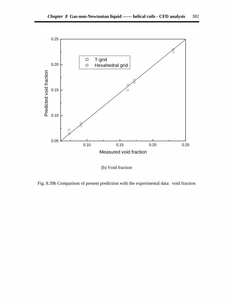
Chapter 8 Gas-non-Newtonian liquid ------ helical coils - CFD analysis 382
0.10 0.15 0.20 0.250.05
0.10
0.15
0.20
0.25
Pred
icte
d vo
id fr
actio
n
Measured void fraction
T-grid Hexahedral grid
(b) Void fraction
Fig. 8.39b Comparison of present prediction with the experimental data: void fraction
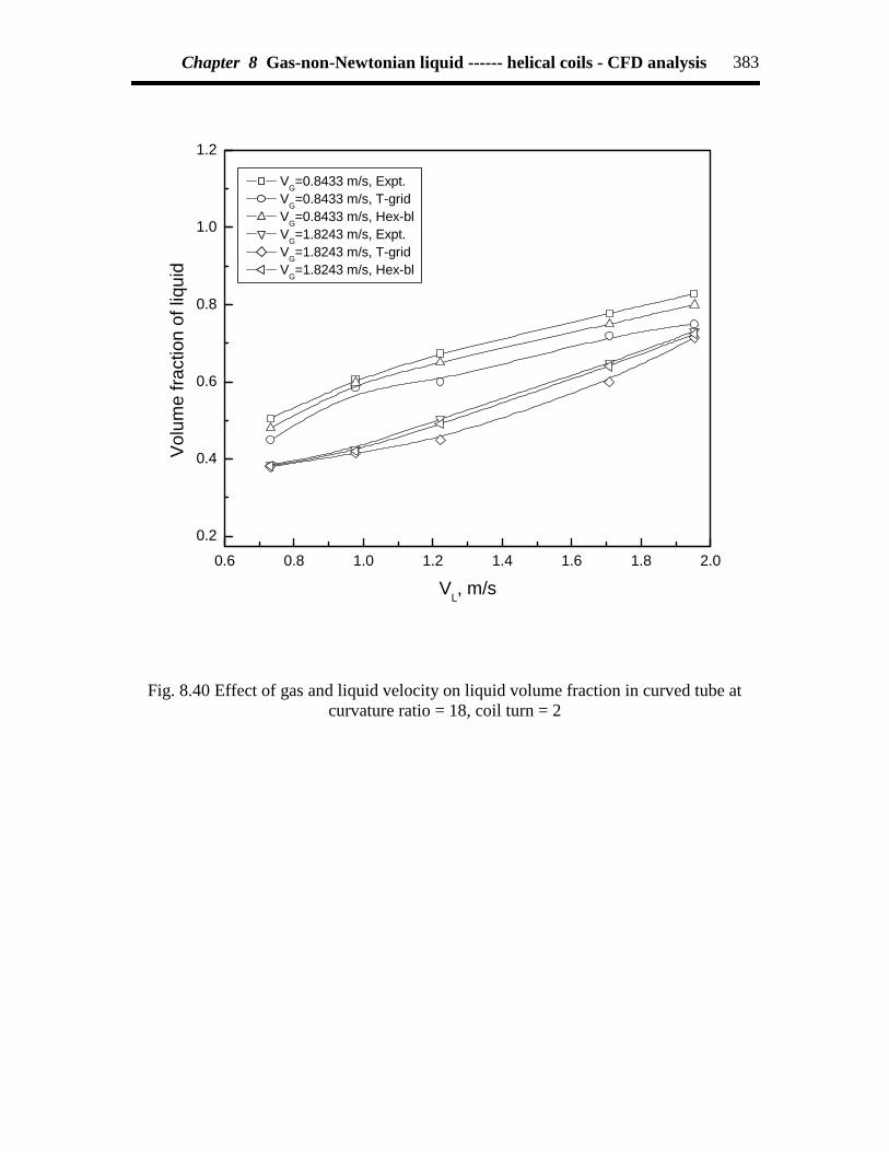
Chapter 8 Gas-non-Newtonian liquid ------ helical coils - CFD analysis 383
0.6 0.8 1.0 1.2 1.4 1.6 1.8 2.0
0.2
0.4
0.6
0.8
1.0
1.2
Volu
me
fract
ion
of li
quid
VL, m/s
VG=0.8433 m/s, Expt. VG=0.8433 m/s, T-grid VG=0.8433 m/s, Hex-bl VG=1.8243 m/s, Expt. VG=1.8243 m/s, T-grid VG=1.8243 m/s, Hex-bl
Fig. 8.40 Effect of gas and liquid velocity on liquid volume fraction in curved tube atcurvature ratio = 18, coil turn = 2

Chapter 8 Gas-non-Newtonian liquid ------ helical coils - CFD analysis 384
-1.0 -0.5 0.0 0.5 1.0
0.0
0.2
0.4
0.6
0.8
1.0
1.2
1.4
1.6V/
V avg
r/a
VG=1.8243 m/s, Expt. VG=1.8243 m/s, T-grid VG=1.8243 m/s, Hex,bl VG=0.8433 m/s, Expt. VG=0.8433 m/s, T-grid VG=0.8433 m/s, Hex-bl
Fig. 8.41 Effect of gas and liquid velocity on development of axial velocity profile incurved tube at curvature ratio 18, coil turn = 2, VL=1.9531 m/s, in horizontal centerline
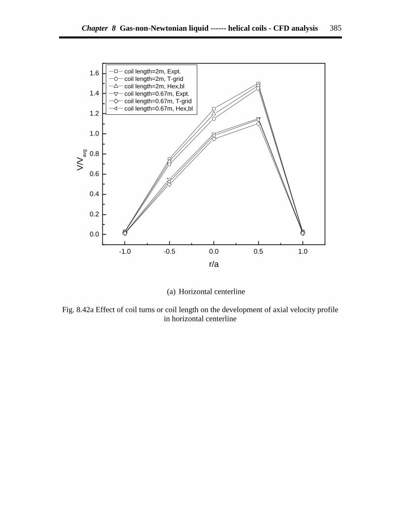
Chapter 8 Gas-non-Newtonian liquid ------ helical coils - CFD analysis 385
-1.0 -0.5 0.0 0.5 1.0
0.0
0.2
0.4
0.6
0.8
1.0
1.2
1.4
1.6V/
V avg
r/a
coil length=2m, Expt. coil length=2m, T-grid coil length=2m, Hex,bl coil length=0.67m, Expt. coil length=0.67m, T-grid coil length=0.67m, Hex,bl
(a) Horizontal centerline
Fig. 8.42a Effect of coil turns or coil length on the development of axial velocity profilein horizontal centerline

Chapter 8 Gas-non-Newtonian liquid ------ helical coils - CFD analysis 386
-1.0 -0.5 0.0 0.5 1.0
0.0
0.5
1.0
1.5
2.0
V/V av
g
r/a
coil length=2.0m, Expt. coil length=2.0m, T-grid coil length=2.0m, Hex,bl coil length=0.67m, Expt. coil length=0.67m, T-grid coil length=0.67m, Hex,bl
(b) Vertical centerline
Fig. 8.42b Effect of coil turns or coil length on the development of axial velocity profilein vertical centerline

Chapter 8 Gas-non-Newtonian liquid ------ helical coils - CFD analysis 387
-1.0 -0.5 0.0 0.5 1.0-0.2
0.0
0.2
0.4
0.6
0.8
1.0
1.2
1.4
1.6
1.8
2.0
V/V
avg
r/a
Symbol Angle (deg) 0 30 60 90 120 150 240 330
(a) Horizontal centerline
Fig. 8.43a Effect of angle on the development of axial velocity profile in horizontalcenterline

Chapter 8 Gas-non-Newtonian liquid ------ helical coils - CFD analysis 388
-1.0 -0.5 0.0 0.5 1.0-0.2
0.0
0.2
0.4
0.6
0.8
1.0
1.2
1.4
1.6
V/V av
g
r/a
Symbol Angle (deg) 0 30 60 90 120 150 240 330
(b) Vertical centerline
Fig. 8.43b Effect of angle on the development of axial velocity profile in verticalcenterline

Chapter 8 Gas-non-Newtonian liquid ------ helical coils - CFD analysis 389
-1.0 -0.5 0.0 0.5 1.0
0.0
0.5
1.0
1.5V/
V avg
r/a
curvature ratio=18, Expt. curvature ratio=18, T-grid curvature ratio=18, Hex, bl curvature ratio=28, Expt. curvature ratio=28, T-grid curvature ratio=28, Hex, bl
(a) Horizontal centerline
Fig. 8.44a Effect of curvature ratio on the development of axial velocity profile inhorizontal centerline at VG = 0.8433 m/s, VL = 1.9531 m/s

Chapter 8 Gas-non-Newtonian liquid ------ helical coils - CFD analysis 390
-1.0 -0.5 0.0 0.5 1.0
0.0
0.5
1.0
1.5
V/V av
g
r/a
curvature ratio=18, Expt. curvature ratio=18, T-grid curvature ratio=18, Hex,bl curvature ratio=28, Expt. curvature ratio=28, T-grid curvature ratio=28, Hex, bl
(b) Vertical centerline
Fig. 8.44b Effect of curvature ratio on the development of axial velocity profile invertical centerline, at VG = 0.8433 m/s, VL = 1.9531 m/s
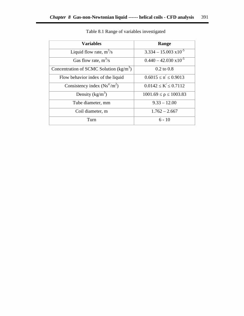
Chapter 8 Gas-non-Newtonian liquid ------ helical coils - CFD analysis 391
Table 8.1 Range of variables investigated
Variables Range
Liquid flow rate, m3/s 3.334 – 15.003 x10⁻⁵
Gas flow rate, m3/s 0.440 – 42.030 x10⁻⁵
Concentration of SCMC Solution (kg/m3) 0.2 to 0.8
Flow behavior index of the liquid 0.6015 ≤ n/ ≤ 0.9013
Consistency index (Nsn'/m2) 0.0142 ≤ K/ ≤ 0.7112
Density (kg/m3) 1001.69 ≤ ρ ≤ 1003.83
Tube diameter, mm 9.33 – 12.00
Coil diameter, m 1.762 – 2.667
Turn 6 - 10

Chapter 8 Gas-non-Newtonian liquid ------ helical coils - CFD analysis 392
Table 8.2 Comparison of the experimental and CFD analysis data for frictional pressuredrop across the coil for liquid (SCMC) concentration of 0.8 kg/m3
Sl.No. Air flowrate
Qgx105
m3/s
Two-phasefrictional
pressure drop(Pftpc/L)Expt.
kPa/m
Two-phasefrictional
pressure drop(Pftpc/L)CFD
Hex GridkPa/m
Two-phasefrictional
pressure drop(Pftpc/L)CFD, T-
GridkPa/m
Liquid flow rate, Ql :11.67x10⁻⁵ m3/s, Dt /Dc: 0.0431
1234
0.33230.50510.62511.0732
8.11888.58718.864
10.045
8.18.5258.8659.98
7.98.28.59.7
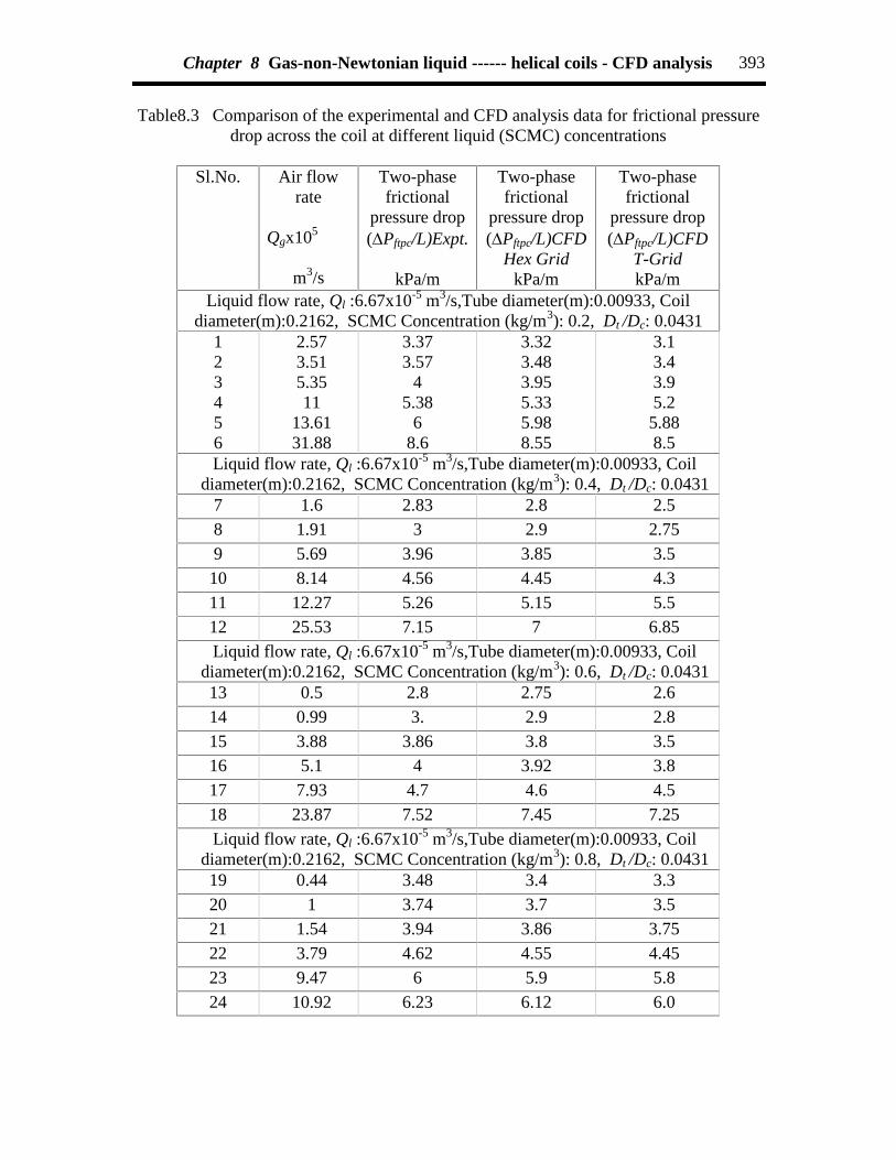
Chapter 8 Gas-non-Newtonian liquid ------ helical coils - CFD analysis 393
Table8.3 Comparison of the experimental and CFD analysis data for frictional pressuredrop across the coil at different liquid (SCMC) concentrations
Sl.No. Air flowrate
Qgx105
m3/s
Two-phasefrictional
pressure drop(Pftpc/L)Expt.
kPa/m
Two-phasefrictional
pressure drop(Pftpc/L)CFD
Hex GridkPa/m
Two-phasefrictional
pressure drop(Pftpc/L)CFD
T-GridkPa/m
Liquid flow rate, Ql :6.67x10⁻⁵ m3/s,Tube diameter(m):0.00933, Coildiameter(m):0.2162, SCMC Concentration (kg/m3): 0.2, Dt /Dc: 0.0431
123456
2.573.515.3511
13.6131.88
3.373.57
45.38
68.6
3.323.483.955.335.988.55
3.13.43.95.2
5.888.5
Liquid flow rate, Ql :6.67x10⁻⁵ m3/s,Tube diameter(m):0.00933, Coildiameter(m):0.2162, SCMC Concentration (kg/m3): 0.4, Dt /Dc: 0.0431
7 1.6 2.83 2.8 2.58 1.91 3 2.9 2.759 5.69 3.96 3.85 3.5
10 8.14 4.56 4.45 4.311 12.27 5.26 5.15 5.512 25.53 7.15 7 6.85Liquid flow rate, Ql :6.67x10⁻⁵ m3/s,Tube diameter(m):0.00933, Coil
diameter(m):0.2162, SCMC Concentration (kg/m3): 0.6, Dt /Dc: 0.043113 0.5 2.8 2.75 2.614 0.99 3. 2.9 2.815 3.88 3.86 3.8 3.516 5.1 4 3.92 3.817 7.93 4.7 4.6 4.518 23.87 7.52 7.45 7.25Liquid flow rate, Ql :6.67x10⁻⁵ m3/s,Tube diameter(m):0.00933, Coil
diameter(m):0.2162, SCMC Concentration (kg/m3): 0.8, Dt /Dc: 0.043119 0.44 3.48 3.4 3.320 1 3.74 3.7 3.521 1.54 3.94 3.86 3.7522 3.79 4.62 4.55 4.4523 9.47 6 5.9 5.824 10.92 6.23 6.12 6.0
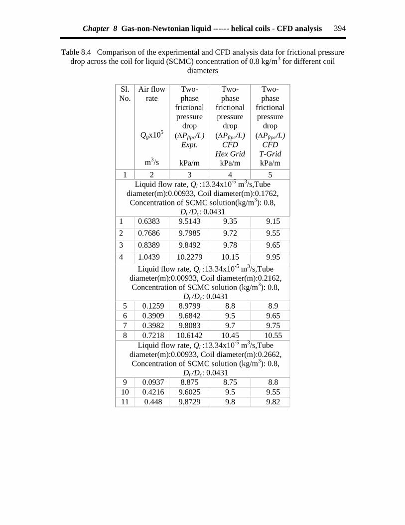
Chapter 8 Gas-non-Newtonian liquid ------ helical coils - CFD analysis 394
Table 8.4 Comparison of the experimental and CFD analysis data for frictional pressuredrop across the coil for liquid (SCMC) concentration of 0.8 kg/m3 for different coil
diameters
Sl.No.
Air flowrate
Qgx105
m3/s
Two-phase
frictionalpressure
drop(Pftpc/L)
Expt.
kPa/m
Two-phase
frictionalpressure
drop(Pftpc/L)
CFDHex Grid
kPa/m
Two-phase
frictionalpressure
drop(Pftpc/L)
CFDT-GridkPa/m
1 2 3 4 5Liquid flow rate, Ql :13.34x10⁻⁵ m3/s,Tube
diameter(m):0.00933, Coil diameter(m):0.1762,Concentration of SCMC solution(kg/m3): 0.8,
Dt /Dc: 0.04311 0.6383 9.5143 9.35 9.15
2 0.7686 9.7985 9.72 9.55
3 0.8389 9.8492 9.78 9.65
4 1.0439 10.2279 10.15 9.95
Liquid flow rate, Ql :13.34x10⁻⁵ m3/s,Tubediameter(m):0.00933, Coil diameter(m):0.2162,Concentration of SCMC solution (kg/m3): 0.8,
Dt /Dc: 0.04315 0.1259 8.9799 8.8 8.96 0.3909 9.6842 9.5 9.657 0.3982 9.8083 9.7 9.758 0.7218 10.6142 10.45 10.55
Liquid flow rate, Ql :13.34x10⁻⁵ m3/s,Tubediameter(m):0.00933, Coil diameter(m):0.2662,Concentration of SCMC solution (kg/m3): 0.8,
Dt /Dc: 0.04319 0.0937 8.875 8.75 8.8
10 0.4216 9.6025 9.5 9.5511 0.448 9.8729 9.8 9.82

References
References
Abbott, M. B. and Basco, D. R., Computational fluid dynamics: an introduction forengineers, Longman Group UK Limited (1989).
Akagawa, N., Sakaguchi, T. and Udea, M., Study on gas-liquid two-phase flow inhelically coiled tubes, Bull. JSME, 14, 564-571 (1971).
Al-Rafai, W., Tridimas, Y. D. and Woolley, N . H., A study of turbulent flows in pipebends, Proc. Ins. Mech. Engers., 204, 399-408 (1990).
Alizadehdahkel, A., Rahimi, M, Sanjari, J. and Alsairafi, A. A., CFD and artificial neuralnetwork modeling of two-phase flow pressure drop, Int. Commun. Heat MassTransfer, 36, 850– 856 (2009).
Anwer, M. and So, R. M. C., Rotation effects on a fully-developed turbulent pipe flow,Expt. Fluids, 8, 33-40 (1989).
Anwer, M., So, R. M. C. and Lai, Y.G, Perturbation by and recovery from bend curvatureof a fully developed turbulent pipe flow, Phys Fluids, A1, 1387-1397 (1989).
Anwer, M., So, R. M. C., Swirling turbulent flow through a curved pipe Part I; effect ofswirl and bend curvature, Expt. Fluids, 14, 85-96 (1993).
Awwad, A., Xin, R. C., Dong, Z. F., Ebadin, M. A. and Soliman, H. M., Measurment andcorrelation of the pressure drop in air-water two-phase in horizontal helicoidalpipes, Int. J. Multiphase Flow, 21, 607-619 (1995).
Azzi, A., Friedel, L, and Balaadi, S., Two-phase gas/liquid flow pressure loss in bends,Forsch. Im Ingenieurwesen, 65(10), 309-318 (2000).
Azzi, A., Friedel, L., Kibbona, R. and Shannak, B., Reproductive accuracy of two-phaseflow pressure loss correlations for vertical 90o bends, Forsch. im Ingenieurwesen,67(10), 109-166 (2002).
Azzola, J., Humphery, J. A. C, Iacovides, H. and Launder, B. E., Developing turbulentflow in a U- bend of circular cross-section : measurement and computation,Trans. J. Fluid Engg., ASME, 108, 214-221 (1986).
Bandala-Rocha, M. R., Macedo, R. C., Ramirez and J. F., Velez-Ruiz, Valuación decoeficientes de fricción en el transporte de fluidos no-Newtonianos, InfórmacionTechnológica, 16, 73-80 (2005).
Bandyopadhyay, T. K., Studies on non-Newtonian and gas-non-Newtonian liquid flowthrough horizontal tube and piping components, Ph. D., Thesis, C. U. (2002).
References 401
Bandyopadhyay, T. K. and Das, S. K., Non-Newtonian pseudo plastic liquid flowthrough small diameter piping components, J. Pet. Sci. Engg., 55, 156–166(2007).
Bandyopadyay, T. K., Banerjee, T. K. and Das, S. K., Gas-non-Newtonian liquid flowthrough elbows, Chem. Engg. Comms., 182:1, 21-33 (2000).
Banerjee, T. K., Das, M. and Das, S. K., Non-Newtonian liquid flow through globe andgate valves, Can. J. Chem. Engg., 72, 207-211 (1994).
Banerjee, S., Rhodes, E., and Scott, D. S., Film inversion of co-current two-phase flow inhelical coils, AIChE J., 13 189-191(1967).
Berger, S. A., Talbot, A. and Yao, L. S., Flow in curved pipes, Ann. Rev. Fluid Mech.,15, 461-512 (1983).
Bergstrom, D. J., Bender, T., Adamopoulos, G. and Postlethwaite, J., Numericalprediction of wall mass transfer rates in turbulent flow through a 90o two-dimensional bend, Can. J. Chem. Engg., 76, 728-737 (1998).
Berrouk, A. B. and Laurence, D., Stochastic modeling of aerosol deposition for LES of900 bend turbulent flow, Int. J. Heat and Fluid Flow, 29, 1010-1028 (2008).
Biswas, A. B., Studies on two-phase gas-non-Newtonian liquid flow through helicalcoils, Ph. D., Thesis, C. U. (2006).
Biswas, A. B. and Das, S. K., Two-phase frictional pressure drop of gas-non-Newtonianliquid flow through helical coils in vertical orientation, Chem. Engg. Proc., 47(5),816-826 (2008).
Breuer, M., Baytekin, H. T. and Matida, E. A., Prediction of aerosol deposition in 900
bends using LES and an efficient Lagrangian tracking method, J. Aerosol Sci., 37,1407-1428 (2006).
Brockmann, J. E., Sampling and transport of aerosol, in aerosol measurement: principles,techniques, and applications, in Baron P. A.and Willeke K., editors, New York,Van Nostrand Reinhold (1993).
Brown, Gary, Use of CFD to predict and reduce erosion in an Industrial slurry pipingsystem, 5th Int. Conf. on CFD in the process industries CSIRO, Melbourne,Australia, 13-15 December (2006).
Bruce, J. M., Two-phase flow in straight pipe and 900 bends, Ph. D. Thesis, Univ.Aberdeen (1971).
Castillo, J. R., Study of two-phase flow in pipe bends, M. Sc. Thesis, MIT (1957).
References 402
Chen, L., Steam-water two-phase flow frictional pressure drop in straight tubes, in X.Chen(Ed.), Selected Papers of Multiphase Flow and Heat Transfer, Paper 7, Xian Jiaotong University Press., 7.1-7.6 (1982).
Chen, Y. I., Wang, C. C. and Lin, S. Y., Measurement and correlations of frictionalsingle-phase and two-phase pressure drops of R-410A flow in small U-type returnbends, Int. J. Heat Mass Transfer, 47, 2241–2249 ( 2004).
Chen, X. J. and Zhou, F. D., An investigation of flow pattern and frictional pressure dropcharacteristics of air-water two-phase flow in helical coils, in Proc. of the fourthMiami Int. Conf. on alternate energy sources, 120-129 (1981).
Cheng, G. C. and Farokhi, S., On tutbulent flows dominated by curvature effects, J.Fluids Engg., 114, 52-57 (1992).
Chenoweth, J. M. and Martin, M. W., Turbulent two-phase flow, Pet. Ref., 34(10), 151-155 (1955).
Chisholm, D. Two-phase Flow in Bends, Int. J. Multiphase Flow , 6, 363–367 (1980).
Cohen, M. I., An investigation of pressure drop in a two-phase two-component, flow inbends, M. Sc. Thesis, MIT (1957).
Chung T. J., Computational fluid dynamics, Cambridge University Press, Cambridge,(2002).
Chung, K. Y., Brewster, M. E. and Belfort, B., Dean Vortices with wall flux in a curvedchannel membrane systems, 2 - The velocity field, AIChE J., 42(2), 347-358(1996).
Czop, V., Barbier, D. and Dong, S., Pressure drop, void fraction and shear strssmeasurements in an adiabatic two-phase flow in a coiled tube, Nucl. Eng. Des.,149, 323-333 (1994).
Das, S. K., Water flow through helical coils in turbulent condition, in Multiphase Reactorand Polymerization System Hydrodynamics, N. P. Cheremisinoff Editor, GulfPublication USA, Ch. 17, 379-403 (1996).
Das, S. K., Biswas, M. N. and Mitra, A. K., Pressure losses in Two-phase Gas-non-Newtonian liquid flow in horinzontal tube, J. Pipelines, 7, 307-325 (1989).
Das, S. K., Biswas, M. N. and Mitra, A. K., Friction factor for Gas-non-NewtonianLiquid Flow in Horizontal Bends, Can. J. Chem. Engg., 69, 179–187 (1991a).

References 403
Das, S. K., Biswas, M. N. and Mitra, A. K., Non-Newtonian liquid flow in bends, Chem.Eng. J., 45, 165-171 (1991b).
Davis, J. A. and Stewart, M., Geometry effects when using CFD analysis as a design toolto predict the control valve., Dev. Theo. Appl. Mechanics, 19, 38-45 (1998).
Dean, W. R., Note on the motion of fluid in a curved pipe, Philos. Mag., 20, 208-223(1927).
Dean, W.R., Fluid motion in a curved channel, Proc. R. Soc. London, Vol. 121, 402-420(1928a).
Dean, W. R., The Stream-line motion in curved pipes, Philos. Mag., 30, 673- 693,(1928b).
Deobold T. L., An experimental investigation of two-phase pressure losses in pipeelbows, M. Sc., Univ. Idaho, Chem., Eng. Rept., HW-SA, 2564 (1962).
Domanski, P. A. and Christian, J. L. H., An improved correlation for two-phase pressuredrop of R-22 and R-410A in 180o return bends, Appl. Thermal Eng., 28, 793–800(2008).
Edwards, M. F., Jadallah, M. S. and Smith, R., Head losses in pipe fittings at lowReynolds numbers, Chem. Eng. Res. Dev., 63, 43-50 (1985).
Edwards, J. K., McLaury, B. S. and Shirazi, S. A., Supplementing a CFD code witherosion prediction capabilities, In Proc. of ASME FEDSM'98: ASME FluidsEngineering Division Summer Meeting, Washington D.C., June, 245 1-7 (1998).
Enayet, M. M., Gibson, M. M., Taylor, A. M. K. P. and Yianneskis, M., Laser–dopplermeasurements of laminar and turbulent flow in a pipe bend, Int. J. Heat FluidFlow, 3, 213-219( 1982).
Engineering Science Data Unit Ltd., Pressure losses in curved duct, single bends, ESDU,Rept. No. 77008 (1977).
Etemad, S. and Sunden, S., Numerical analysis of turbulent convective heat transferprocesses in a square-sectioned U-bend duct, 15th Australasian Fluid MechanicsConf., Sydney, Australia, 13-17 Dec. (2004).
Eustice, J., Flow of water in curved pipes, Proc. R. Soc. London, 84, 107-118, (1910).
Famiyesin, O. O. R., Oliver, K. D. and Rodger, A. A., Semi-empirical equations forpipeline designby the finite element method, Comp. & Structures, 80, 1369-1382(2002).

References 404
Faruki, N. M., and Parker, J. D., A visual study of air-water mixtures flowing insideserpentine tubes, Proc. 5th Int. Heat Transfer Conf., JSME, Tokyo, B5.5, pp 205-209, (1974).
Ferziger, J. H. and Peric, M, Computational methods for fluid dynamics, Springer, Berlin,(1997).
Fitzsimmons, P. E., Two phase pressure drop in pipe components, General electric Res.Rept., HW-80970, Rev. 1 (1964).
Fluent Users Guide, Version 6.2, Fluent India, Pune (2006).
Fluent Users Guide, Version 6.3, Fluent India, Pune (2008).
Flow Meters – Their theory and application, Report of the ASME Research Committee onFluid Meter, ASME, New York, 5th Ed., (1959).
Gadiyar, N. and Das, S. K., Pressure losses in two-phase air water flow in orifices, Ind. J.Technol, 31, 811-814(1993).
Gao, H., Gu, Y. J. and Guo, L. J., Numerical study of stratified oil-water two-phaseturbulent flow in a horizontal tube, Int. J. Heat Mass Transfer, 46, 749-754(2003).
Geary, D. F., Return bend pressure drop in refrigeration systems, ASHRAE Trans. 81(1),250–264 (1975).
Gelfgat, A. Yu., Yarin, A. I. and Bar-Yoseph, P. Z., Dean vortices-induced enhancementof mass transfer through an interface separating two immiscible liquids, Phys.Fluids, 15(2), 330-347 (2003).
Guan, X. and Martonen, T. B. Flow transition in bends and applications to airways, J.Aero. Sci., 31, 831-847 (2000).
Guo, L. and Chen, X., An experimental investigation of the frictional pressure drop ofsteam-water two-phase flow in helical coils, Int. J. Heat Mass Transfer, 44(14),2601-2610 (2001).
Guo, L. J., Chen, X. J., Zhang, S. K. and Feng, Z. P., Correlation for predicting pressuredrop of single and two-phase flow through horizontally helically coiled tubes, inProc. 3rd Int. Sym. Multiphase Flow and Heat Transfer, 514-52, (1994).
Hart, J., Ellenberger, J., and Hamersma, P. J., Single and two-phase flow throughhelically coiled tubes, Chem. Engg. Sci., 43, 775-783 (1988).

References 405
Hidayat, M. and Rasmuson, A., Numerical investigation of gas-solid flow in a U-bend,Proc. 13th Int. Drying Sym., A, 424-433, Bejing, China, IDS’ (2002).
Hoang, K. and Davis, M.,R., Flow Structure and Pressure Loss for Two Phase Flow inReturn Bends, 7th Annual/Energy-Sources Technology Conf. and Exhibit, NewOrleans, U.S.A., Paper no. 84-FE-1, Feb. 11–17 (1984).
Hooper, W. B., Piping design, fittings, pressure drop, Encyclopedia of ChemicalProcessing and Design, (Ed. J. J. Mcketta), 39, 19-27 (1991).
IS: 10605 – 1983, Steel globe valves (flanged and butt welded ends) for petroleum,petrochemical and allied industries (first revision), Bureau of Indian Standard,(1983).
IS: 11335 – 1984, Cast Iron Gate valves, Bureau of Indian Standard, (1984).
Ito, H., Friction factors for turbulent flow in curved pipes, ASME J. of Basic Engg., 81,123-134 (1959).
Jayanti, S., Hewitt, G. F. and Kightley, J. R., Fluid flow in curved ducts, Int. J. Num.Methods in Fluids, 10, 567-589 (1990).
Jayakumar, J. S., Mahajani, S. M., Mandal, J. C., Iyer, K. N. and Vijayan, P. K., Thermalhydraulic characteristics of air-water two-phase flows in helical pipes, Chem.Engg. Res. Deg., 88, 501-512 (2010).
Joshi, J. B. and Ranade, V. V., Computational fluid dynamics for designing processequipment: expectation, current status, and path forward, Ind. Eng. Chem. Res.,42, 1115-1128 (2003).
Kim, J. and Simon, T. W., Measurements of the turbulent transport of heat andmomentum in convexly curved boundary layers : effects of curvature, recoveryand free-stream turbulence, J. Turbomachinery, 110, 81-87 (1988).
Kuan, B., Yang, W. and Solnordal, C., CFD simulation and experimental validation ofdilute particulate turbulent flows in a 900 duct bend, 3rd Int. Conf. on CFD in theMinerals and Process Industries CSIRO, Melbourne, Australia 10-12 December(2003).
Kumar, A., Kaushal, D. R. and Kumar, U., Bend Pressure drop experiments comparedwith Fluent, Eng. Computational Mech., 161, 35-42 (2008).
Lockhert, R. W. and Martinelli, R. C., Proposed correlation of data for isothermal two-phase two component flow in pipes, Chem. Engg. Prog., 45, 39 (1949).

References 406
Maddock, C., Lacey, P. M. C. and Patrick, M. A., The structure of two-phase flow in acurved pipe in: I. ChemE Symp. Ser., 38, Paper J2, pp. 1-22 (1974).
Mandal, S. N. and Das, S. K., Pressure Losses in Bends during Two-Phase Gas-Newtonian Liquid Flow, Ind. Eng. Chem. Res., 40, 2340–2351 (2001).
Mandal, S. N. and Das, S. K., Gas-Liquid flow through helical coils in verticalorientation, Ind. Eng. Chem. Res., 42, 3487–3494 (2003).
Manzar, M. A. and Shah, S. N., Particle distribution and erosion during the flow ofNewtonian and non-newtonian slurries in straight and coiled pipes, Engg.Applications Comp. Mech., 3, 296-320 (2009).
Marn, J. and Ternik, P., Laminar flow of a shear-thickening fluid in a 90o pipe bend,Fluid Dynamics Res., 38, 295-312 (2006).
Mishra, P. and Gupta, S. N., Momentum transfer in curved pipes. 2. Non-Newtonianfluids, Ind. Eng. Chem. Process Dev., 18(1), 137-142 (1979).
Moulin, Ph., Veyreth, D. and Charbit, D. F., Dean vortices: comparison of numericalsimulation of shear stress and improvement of mass transfer in membraneprocesses at low permeation fluxes, J. Membr. Sci., 183, 149-162 (2001).
Owhadi, A., Bell, K. J. and Crain, B., Forced convection boiling inside helically coiledtubes, Int. J. Heat Mass Transfer, 11, 1779-1793 (1968).
Patankar, S. V., Numerical heat transport and fluid flow, Taylor and Francis, New York,(1989).
Pierre, B., Flow resistance with boiling refrigerants – Part II: Flow resistance in returnbends, ASHRAE J., 73–77 (1964).
Polizelli, M. A., Menegalli, F. C., Telis, V. R. N. and Telis-Romero, J., Friction losses invalves and fittings for power-law fluids, Brazilian J. Chem. Engg., 20, 455-463(2003).
Pruvost, J., Legrand, J. and Legentilhomme, P., Numerical investigation of bend andtours flow, part I : effect of swirl motion on flow structure in U-bend, Chem.Engg. Sci, 59, 3345-3357 (2004).
Pui, D. Y. H., Romay-Novas, F. and Liu, B.Y. H., Experimental study of particledeposition in bends of circular crossection, Aerosol Sci. Technol., 7, 301-315(1987).
Ranade, V. V., Computational flow modelling for chemical reactor engineering,Academic Press: London (2002).
References 407
Rowe, M., Measurements and computations of flow in pipe bends, J. Fluid Mech., 43(4),771-783 (1970).
Roorda, O., Computer simulation helps reduce pressure loss, Water, Engg. Mag., 40, 22-24 (1998).
Samanta, A. K., Banerjee, T. K. and Das, S. K., Pressure losses in orifices for the flow ofgas-non-Newtonian liquid, Can. J. Chem. Engg., 77, 579-583 (1999).
Santini, L., Cioncolini, A., Lombardi, C. and Ricotti, M., Two-phase pressure drops in ahelically coiled steam generator, Int. J. Heat Mass transfer, 51, 4926-4939(2008).
Saxena, A. K., Nigam, K. D. P., Schumpe, A., Deckwer, W. D., Liquid phase residencetime distribution for two-phase flow in coiled tubes, Can. J. Chem. Eng., 74, 861-866 (1996).
Sekoda, K., Sato, Y. and Karyia, S., Horizontal two-phase air-water flow characteristicsin the disturbed region due to a 90 degree bend, J. Jpn. Soc. Mech. Eng., 35(289),2227-2333 (1969).
Schiller, L. and Naumann, Z., A drag coefficient correlation, Zait Ver Deutsch Ing, 77,318-325 (1935).
Shah, N. S. and Jain, S., Coiled tubing erosion during hydraulic fracturing slurry flow,Wear, 264, 279-290 (2008).
Shah, R. K. and Joshi, S. D., Convective heat transfer in curved ducts, in Handbook ofsingle-phase convective heat transfer, Kakac, S., Shah, R. K., & Aung, W. (eds).(Wiley interscience, New York), Chapter 3, p. 1238 (1987).
Sierra-Espinosa, F. Z., Bates, C. J. and O’Dherty T., urbulent flow in a 90o pipe junctionPart 1 : decay of fluctuations upstream the flow bifurcation, Comp. & Fluids, 29,197-213 (2000a).
Sierra-Espinosa, F. Z., Bates, C. J. and O’Dherty T., urbulent flow in a 90o pipe junctionPart 2 : reverse flow at the branch exit, Comp. & Fluids, 29, 215-233 (2000b).
So, R. M. C., Zhang, H. S. and Lai, Y. G., Secondary cells and separation in developinglaminar curved-pipe flows, Theor. Comput. Fluid Dyn., 3, 141-162 (1991).
Spedding, P. I., Chen, J. J. J. and Nguyen, V. T., Pressure drop in two phase gas-liquidflow in inclined pipes, Int. J. Multiphase flow, 8, 407-431 (1982).

References 408
Spedding, P. L., Benard, E. and McNally, G. M., Fluid flow through 90 degree bends,Dev. Chem. Eng. Min. Process, 12, 107-128 (2004).
Spedding, P. L. and Benard, E., Gas-liquid two-phase flow through a vertical 900 elbowbend, Exp. Thermal Fluid Sci., 31, 761-769 (2007).
Straub, L. G. and Silberman, E., Air-water mixture flow through orifices, bends and otherfittings in a horizontal pipe, St Anthony falls, Hydraulic Lab., Univ. MinnesotaRept., 63 (1960).
Struiver, W., Two phase fluid flow through bends and preliminary study of bends andpreliminary study of pressure drop along pipe, Dominion physical lab,Newzeland, ANL, R257, 6734-1694 (1955).
Sudo, K., Sumida, M. and Hibara, H., Experimental investigation on turbulent flow in acircular-sectioned 90-degrres bend, Expt. Fluids, 25, 42-49 (1998).
Sudo, K., Sumida, M. and Hibara, H., Experimental investigation on turbulent flowthrough a circular sectioned 1800 bend, Expt. Fluids, 28, 51-57 (2000).
Supa-Amornkul, S., Steward, F., R. and Derek, H. L., Modeling Two-Phase Flow in PipeBends, J. Press. Vessel Technol., 127, 204-209 (2005).
Telis-Romero, J., Gratao, A. C., Gacia-Cruz, C. H., Telis, V.R.N., Determinacao decoefficients de perda de carga atraves de valvulas e accessoris no escoamentolaminar de fluidos naONewtonianos, Ciencia & Engenharia, 9, 78-82 (2000).
Thomson, J., On the origin of windings of rivers in alluvial plains, with remarks on theflow of water round bends in pipes, Proc. R. Soc. London, 25, 5-8 (1876).
Tiwari, P., Antal, S. P., Burgoyne, A., Belfort, G. and Podowski, M. Z., Multifiedcomputational fluid dynamics model of particulate flow in curved circular tubes,Theor. Comput. Fluid Dyn., 18, 205-220 (2004).
Tunstall, M. J. and Harvey, J. K., On the effect of a sharp bend in a fully developedturbulent pipe-flow, J. Fluid. Mech., 34, 595-608 (1968).
Turian, R. M., Ma, T. W., F. L. G., Hsu, Sung, M. D. J. and Plackmann, G. W., Flow ofconcentrated non-Newtonian slurries : 2. friction losses in bends, fittings, valvesand venture meters, J. Multiphase Flow, 24, 243-269 (1998).
Unal, H. C., Gasself, V. M. I. G., Versalt, P. M. and Dryout, Von’t, Two-phase flowpressure drop in sodium heated helically coiled steam generators tubes at elevatedpressure, Int. J. Heat Mass Transer, 24, 285-298 (1981).
References 409
Usui, K., Akoi, S. and Inoue, A., Flow behavior and phase distribution in two-phase flowaround inverted U-bend, J. Nucl. Sci. Technol., 20(11) 33-46 (1983).
Van de Vosse, F. N., Van Steenhoven, A. A., Sregak, A. and Janssen, J. D., A finiteelement analysis of the steady laminar entrance flow in a 90o curved tube, Int. J.Num. Methods in Fluids, 9, 275-287 (1989).
Vashisth, S. and Nigam, K. D. P., Prediction of flow profiles and interfacial phenomenafor two-phase flow in coiled tubes, Chem. Engg. and Proc. Proc. Intensification,48, 452-463 (2009).
Wang, C. C, Chen, I. Y, Yung, Y. W and Chang, Y. J., Two-phase flow pattern in smalldiameter tubes with the presence of horizontal return bend, Int. J. Heat MassTransfer, 46, 2975–2981 (2003).
Wang, C. C, Chen, I. Y. and Huang, P. S., Two-phase slug flow across small diametertubes with the presence of vertical return bend, Int. J. Heat Mass Transfer, 48,2342–2346, (2005).
Wang, J. and Shirazi, S., A CFD based correlation for mass transfer coefficient in elbows,Int. J. Heat Mass Transfer, 44, 1817-1822 (2001).
Watanabe, O., Tajima, O. and Shimoya, O., Flow and heat transfer of gas and liquid two-phase flow in coils, Trans. JSME, 52 (476B), 1857-1864 (1986).
Wilson, R. E., Mcadams, W. H. and Seltzer, M. The flow of fluids through commercialpipelines, IEC, 14, 105-119 (1922).
Wu, B. and Chen, S., CFD simulation of non-Newtonian fluid flow in anaerobicdigesters, Biotecnol. Bioeng. 99, 700-711 (2008).
Xia, B. and Sun, D. W., Applications of computational fluid dynamics (CFD) in the foodindustry: a review, Comp.Eelec. Agriculture, 34, 5-24 (2002).
Xin, R. C., Dong, Z. F. and Ebadin, M. A., Three-Dimensional numerical modelling ofturbulent single-phase and two-phase flow in curved pipes, National HeatTransfer Conference, ASME, 4, 227-233 (1996).
Xin, R. C., Awward, A., Dong, Z. F. and Ebadin, M. A., An experimental study of single-phase and two-phase flow pressure drop in annular helicoidal pipes, Int. J. HeatFluid Flow, 18(5), 482-488 (1997).
Yamamoto, K., Yanase, S. and Yoshida, T., Torsion effect on the flow in a helical pipe,Fluid Dyn. Res., 14, 259-273 (1994).

References 410
Yao, L. S. and Berger, S. A., Entry flow in a coiled pipe, J. Fluid Mech., 67, 177-196(1975).
Zhang, P., Roberts, R. M., Benard, A. and Petty, C. A., Computational study of turbulentsingle phase and multiphase flows in 900 Bends, Proc. of the AICHE 2009 AnnualMeeting , Paper 171080, November (2009).
Zhang, P., Gros, Y., Roberts, R. M. and Benard, A., Modeling of turbulent flow withparticle deposition in curved pipes, Proc. 7th Int. Conf. on Multiphase flow ICMF2010, Tampa, FL USA, May 30-June 4 (2010).
Website
www.cfd-online.com available on 2nd Dec. 2010.
http://www.chemicalvision2020.org/pdfs/compfluid.pdf available on 4th Dec. 2010.