heat transfer in in-tube flow of non-newtonian fluids
TRANSCRIPT

Retrospective Theses and Dissertations Iowa State University Capstones, Theses andDissertations
1978
Heat transfer in in-tube flow of non-NewtonianfluidsSadanand Dattatray JoshiIowa State University
Follow this and additional works at: https://lib.dr.iastate.edu/rtd
Part of the Mechanical Engineering Commons
This Dissertation is brought to you for free and open access by the Iowa State University Capstones, Theses and Dissertations at Iowa State UniversityDigital Repository. It has been accepted for inclusion in Retrospective Theses and Dissertations by an authorized administrator of Iowa State UniversityDigital Repository. For more information, please contact [email protected].
Recommended CitationJoshi, Sadanand Dattatray, "Heat transfer in in-tube flow of non-Newtonian fluids " (1978). Retrospective Theses and Dissertations. 6392.https://lib.dr.iastate.edu/rtd/6392

INFORMATION TO USERS
This was produced from a copy of a document sent to us for microfilming. While the most advanced technological means to photograph and reproduce this document have been used, the quality is heavily dependent upon the quality of the material submitted.
The following explanation of techniques is provided to help you understand markings or notations which may appear on this reproduction.
1. The sign or "target" for pages apparently lacking from the document photographed is "Missing Page(s)". If it was possible to obtain the missing page(s) or section, they are spliced into the film along with adjacent pages. This may have necessitated cutting through an image and duplicating adjacent pages to assure you of complete continuity.
2. When an image on the film is obliterated with a round black mark it is an indication that the film inspector noticed either blurred copy because of movement during exposure, or duplicate copy. Unless we meant to delete copyrighted materials that should not have been filmed, you will find a good image of the page in the adjacent frame.
3. When a map, drawing or chart, etc., is part of the material being photographed the photographer has followed a definite method in "sectioning" the material. It is customary to begin filming at the upper left hand comer of a large sheet and to continue from left to right in equal sections with small overlaps. If necessary, sectioning is continued again—beginning below the first row and continuing on until complete.
4. For any illustrations that cannot be reproduced satisfactorily by xerography, photographic prints can be purchased at additional cost and tipped into your xerographic copy. Requests can be made to our Dissertations Customer Services Department.
5. Some pages in any document may have indistinct print. In all cases we have nimed the best available copy.
University Microfilms
International 300 N. ZEEB ROAD, ANN ARBOR, Ml 48106 18 BEDFORD ROW, LONDON WC1 R 4EJ, ENGLAND

7907255
J054 I , S&DA.MAMD DATTAFRAY HEAT TRANSFER H IM-TUBE FLOW OF N3N-NEWrONI&N FLUIDS.
IOWA STATE UNIVERSITY, PH.D. , 1979
Universi^ Micrcxilms
International 300 N. ZEEB ROAD, Atiirj ARBOR, Ml 48106
PLEASE NOTE: D isser ta t ion con ta ins compute r p r in t -ou ts w i th b roken and i nd is t inc t p r in t . F i Imed as rece i ved .
UNIVERSITY MICROFILMS

Heat transfer in in-tube flow of
non-Newtonian fluids
by
Sadanand Dattatray Joshi
A Dissertation Submitted to the
Graduate Faculty in Partial Fulfillment
The Requirements for the Degree of
DOCTOR OF PHILOSOPHY
Major: Mechanical Engineering
Approved:
In Charge of Majo Work
For the Maj or'Depatiment
Iowa State University Ames, Iowa
1978
Signature was redacted for privacy.
Signature was redacted for privacy.
Signature was redacted for privacy.

il
TABLE OF CONTENTS
Page
NOMENCLATURE xii
CHAPTER I. INTRODUCTION 1
CHAPTER II. REVIEW OF PREVIOUS ANALYTICAL SOLUTIONS 6
Constant Property, Newtonian Heat Transfer 6
Fully developed 6 Thermally developing 6 Thermally and hydrodynamically developing 13 Effects of axial conduction and viscous 13 dissipation
Conclusion 15
- Constant Property, Non-Newtonian Heat Transfer 15
Fully developed 15 Thermally developing 16 Thermally and hydrodynamically developing 19 Conclusion 19
Variable-Property Predictions 20
Variable y, Newtonian Heat Transfer 21
Fully developed 21 Thermally developing 22 Thermally and hydrodynamically developing 25 Conclusion 26
Variable K, Non-Newtonian Heat Transfer 26
Fully developed 26 Thermally developing (UWT) 27 Thermally developing (UHF) 29 Thermally and hydrodynamically developing 33 Conclusion 33
Scope for Further Work and Problem Definition 33
CHAPTER III. NUMERICAL ANALYSIS 36
Introduction 36

iii
Page
Problem Formulation 36
Statement of the problem 36 Governing equations 39 Non-dimensionalized governing equations 41
Finite-Difference Formulation 42
Dufort-Frankel method . , 42 Apparent viscosity formulation 44 Finite-difference equations 45
Consistency, Stability, and Convergence of the 45 Numerical Solution
Consistency 46 Stability 47
Method of Solution 50
Grid spacing in the radial direction 50 Numerical procedure 51 Calculations of viscosities and flow parameters 54 Calculation of heat transfer results 56 Computer code 57
CHAPTER IV. NUMERICAL RESULTS AND DISCUSSION 59
Constant Property Predictions 59
Heat transfer 59 Pressure drop 68 Conclusion 70
Variable Property Predictions 70
Introduction 70 A parameter to account for variable consistency 72 Numerical variables 73 Nusselt number results 74 Development of a variable consistency correction 83 Design procedure 90
Summary and Conclusions 92

iv
Page
CHAPTER V. REVIEW OF EXPERIMENTAL STUDIES 94
Introduction 94
Newtonian Heat Transfer 95
UWT boundary condition 95 UHF boundary condition 100 Conclusions 103
Non-Newtonian Heat Transfer 103
UWT boundary condition 104 UHF boundary condition 106 Conclusion 108
Scope for Further Work 108
CHAPTER VI. EXPERIMENTAL SETUP AND PROCEDURE 109
Introduction 109
Experimental Setup 109
Test loop 109 Test section 113 Measurements and controls 117
Experimental Procedure 119
Test fluids 119 Filling the test loop 122 Operating procedure 123
Data Reduction 125
CHAPTER VII. EXPERIMENTAL RESULTS AND DISCUSSION 128
Experimental Results 128
Statistical Analysis of the Data
Comparison with Previous Data 141
Conclusions 146
CHAPTER VIII. CONCLUSIONS AND RECOMMENDATIONS 148

V
Page
BIBLIOGRAPHY 153
ACKNOWLEDGMENTS 162
APPENDIX A; FINITE-DIFFERENCE EQUATIONS 163
Dufort-Frankel Formulation 163
Comments on Dufort-Frankel Momentum Equation 165
Standard Explicit Finite-Difference Equations 166
APPENDIX B: TRUNCATION ERROR IN THE DUFORT-FRANKEL 168 DIFFERENCE EQUATIONS
APPENDIX C: COMPUTATION OF PRESSURE P ^ 172
APPENDIX D: COMPUTER CODE FOR CHAPTER III 175
APPENDIX E: NUMERICAL PREDICTIONS - CONSTANT PROPERTY 203
APPENDIX F: ANALYSIS OF FULLY DEVELOPED NEWTONIAN 208 HEAT TRANSFER
Problem Formulation 208
Statement of the problem 208 Governing equations 209 Integral equations 210
Method of Solution 212
Results and Discussion 212
APPENDIX G: VARIABLE PROPERTY NUMERICAL PREDICTIONS 225
APPENDIX H: THE PREPARATION OF PSEUDOPLASTIC FLUIDS 231
Method of Preparation 231
APPENDIX I: FLUID FLOW CURVES 233
Experimental Procedure 234
Fluid Degradation 235
Philosophy of time averaging 238

vi
Page
APPENDIX J: WORKING FLUID PROPERTIES 247
Fluid Properties 247
Density 247 Isobaric thermal expansion coefficient 248 Isobaric specific heat 249 Thermal conductivity 249
Consistency Index and Flow Behavior Index 250
Solution I (0.9 percent HEMC, Runs 1 to 10) 250 Solution I (0.9 percent HEMC, Runs 10 to 19) 251 Solution II (1.0 percent HEMC, Runs 1 to 9) 252
APPENDIX K: SAMPLE CALCULATIONS 254
Experimental Parameters 254
Physical dimensions and properties of the tube 254 Measured quantities 254
Experimental Calculations 255
Heat flux calculations 255 Fluid bulk temperature 257 Nusselt number 257 Effective viscosity 258 Dimensionless numbers 258 Comparison with numerical solution 259 Friction factor 262
APPENDIX L: COMPUTER PROGRAM FOR EXPERIMENTAL DATA 265 REDUCTION
APPENDIX M: TABULATION OF EXPERIMENTAL DATA 273
Experimental Results for Solution I (0.9 percent HEMC) 274
Experimental Results for Solution II (1.0 percent HEMC) 281

vii
LIST OF TABLES
Page
Table 2.1. References pertaining to laminar flow in 7 circular tubes
Table 4.1. Comparison of non-Newtonian Nusselt numbers 60 for the fully developed region
Table 4.2. Comparison of pressure gradients 68
Table 4.3. Comparison of Fanning friction factors 69
Table 4.4. Predictions of m in the thermal entrance 83 length
Table 4.5. Fully developed heat transfer predictions 85
Table 5.1. Experimental studies of laminar flow heat 94 transfer in circular tubes
Table 5.2. Experimental studies in horizontal laminar 99 tube flow subjected to UWT boundary condition
Table 6.1. Test section details 113
Table E.l. Flow behavior index, n = 1.0 204
Table E.2. Flow behavior index, n = 0.75 205
Table E.3. Flow behavior index, n = 0.5 206
Table E.4. Flow behavior index, n = 0.25 207
Table F.l. The Newtonian fully developed predictions 215
Table G.I. Flow behavior index, n = 1 226
Table G.2. Flow behavior index, n = 0.75 227
Table G.3. Flow behavior index, n = 0.5 229

viii
Page
Table I.l. Correlations for Solution I (0.9 [ercent HEMC) 237
Table 1.2. Averages of K' and n for Solution I (0.9 240 percent HEMC)
Table 1.3. Correlations for Solution II (1.0 percent 242 HEMC)
Table 1.4. Averages of K' and n for Solution II (1.0 244 percent HEMC)
Table M.l. Experimental variables 274
Table M.2. Experimental results for Solution I 275 (0.9% HEMC)
Table M.3. Experimental variables 281
Table M.4. Experimental results for Solution II 282 (1.0% HEMC)

ix
LIST OF FIGURES
Page
Fig. 1.1 Flow curves of various time-independent 3 fluids (linear axes).
Fig. 2.1 Forced convection heat transfer in a circular 10 tube with uniform wall temperature.
Fig. 2.2 Forced convection heat transfer in a circular 12 tube with uniform wall heat flux.
Fig. 2.3 Forced convection heat transfer in a circular 14 tube with developing flows and a uniform wall temperature.
Fig. 2.4 Forced convection heat transfer in a circular 18 tube for the flow of non-Newtonian fluids.
Fig. 2.5 Local Nusselt number for pipe flow with 31 uniform heat flux and temperature-dependent consistency, (n = 0.50).
Fig. 3.1 Laminar velocity profiles for pseudoplastic 38 fluids.
Fig. 3.2 The finite-difference grid. 43
Fig. 3.3 A flow chart of the computer program. 53
Fig. 4.1 Comparison of present numerical solution 62 with available predictions (n = 1).
Fig. 4.2 Comparison of present numerical solution 63 with available predictions (n = 0.75).
Fig. 4.3 Comparison of present numerical solution 64 with available predictions (n = 0.5).
Fig. 4.4 Comparison of present numerical solution 65 with available predictions (n = 0.25).
Fig. 4.5 Results of the present numerical analysis 66 for laminar in-tube flow of power law fluids.
Fig. 4.6. Comparison of corrected Nusselt numbers for 67 non-Newtonian flow predictions with Newtonian flow predictions.

X
Page
Fig. 4.7 Dependence of Nusselt number on dimensionless 75 distance and viscosity parameter (n = 1).
Fig. 4.8 Dependence of Nusselt number on dimensionless 76 distance and consistency parameter (n = 0.75).
Fig. 4.9 Dependence of Nusselt number on dimensionless 77 distance and consistency parameter (n = 0.5).
Fig. 4.10 Dependence of Nusselt number ratio on viscosity 79 ratio (n = 1).
Fig. 4.11 Dependence of Nusselt number ratio on ratio of 80 consistency indices (n = 0.75).
Fig. 4.12 Dependence of Nusselt number ratio on ratio of 81 consistency indices (n = 0.5).
Fig. 4.13 Dependence of Nusselt ratio on yAT. 86
Fig. 4.14 Dependence of Nusselt ratio on consistency 88 correction factor Cj .
Fig. 4.15 Schematic diagram of the consistency 91 correction.
Fig. 5.1 Comparison of fully developed, heat transfer 101 data for a UHF boundary condition.
Fig. 6.1 Schematic diagram of test loop. 110
Fig. 6.2 Photograph of experimental apparatus. Ill
Fig. 6.3 Schematic diagram of Test Section I. 114
Fig. 6.4 Schematic diagram of Test Section II. 115
Fig. 6.5 Functional diagram of the Data Acquisition 120 System.
Fig. 6.6 Printer, calculator, and A/D converter/scanner 121
Fig. 6.7 Ice-point reference. 121
Fig. 7.1 Plot of experimental heat transfer data. 129

xi
Page
Fig. 7.2 Plot of experimental heàt transfer data with 131 non-Newtonian correction.
Fig. 7.3 Plot of experimental heat transfer data with 132 non-Newtonian correction and temperature-dependent consistency correction.
Fig. 7.4 Plot of experimental heat transfer data with 135 non-Newtonian correction and temperature-dependent consistency correction, with evaluated at wall temperature.
Fig. 7.5 Confidence limits on the data and correlation. 139
Fig. 7.6 Confidence limits on the data and correlation. 140
Fig. 7.7 Comparison of numerical predictions and 143 experimental results.
Fig. 7.8 Comparison of present experimental data and 144 numerical predictions with available experimental data.
Fig. F.l The finite-difference grid for fully developed 213 flow inside a circular tube.
Fig. F.2 A flow chart of the computer program. 214
Fig. I.l Flow curve for 0.9% HEMC solution. 236
Fig. 1.2 Average values for Solution I (0.9% HEMC). 239
Fig. 1.3 Flow curve for 1.0% HEMC solution. 241
Fig. 1.4 Average values for Solution II (1.0% HEMC). 243
Fig. 1.5 Plot of percentage change in effective 246 viscosity against temperature difference.

xii
NOMENCLATURE
a Defined in Eq. (2.40) (Ib sec"/ft )
A Tube surface area (ft )
b Defined in Eq. (2.40) (1/°F)
Cp Isobaric specific heat (Btu/hr°F)
C Defined in Eq. (4.20)
Cg Defined in Eq. (4.20)
Cg Consistency correction (dimensionless)
Cj Defined in Eq. (4.20)
D Inside tube diameter (ft)
D1 Outside tube diameter (ft)
g Gravitational acceleration (ft/sec )
gg Gravitational constant in Newton's law
h Heat transfer coefficient (Btu/hrft °F)
J Conversion constant, 777.66 (ft Ibf/Btu)
k Thermal conductivity (Btu/hrft°F)
kl Thermal conductivity of the tube (Btu/hrft°F)
K Consistency index (Ib sec /ft )
K' Modified consistency index (Ib sec /ft )
L Length of the test section (ft)
Lg Length of the measuring station (ft)
m Mass flow rate (Ib /hr)
" - 2 m Dimensionless mass flow, mp u /y o' a,o
n Flow behavior index (dimensionless)
p Pressure (Ibj/ft )
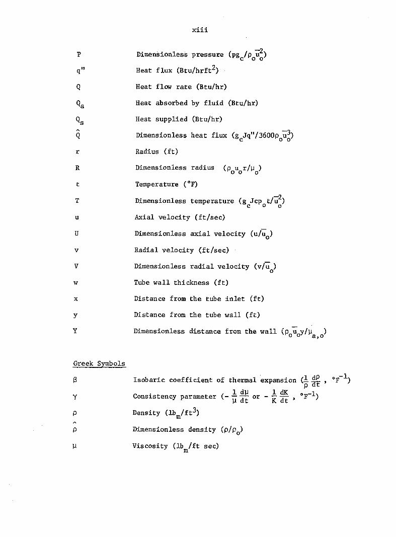
p
q"
Q
Qa
Qs
Q
r
R
t
T
u
U
V
V
w
X
y
Y
Greek Symbols
3
Y
P
P
y
xiii
Dimensionless pressure (pg /p u )
Heat flux (Btu/hrft )
Heat flow rate (Btu/hr)
Heat absorbed by fluid (Btu/hr)
Heat supplied (Btu/hr)
Dimensionless heat flux (g Jq"/3600p i?)
Radius (ft)
Dimensionless radius (pu r/u ) o o o
Temperature (°F)
—2 Dimensionless temperature (g Jcp t/u ) C O o
Axial velocity (ft/sec)
Dimensionless axial velocity (u/u )
Radial velocity (ft/sec)
Dimensionless radial velocity (v/u )
Tube wall thickness (ft)
Distance from the tube inlet (ft)
Distance from the tube wall (ft)
Dimensionless distance from the wall o
Isobaric coefficient of thermal expansion (i , °F ) p dt
Consistency parameter (- or - , °F~ )
Density (Ib /ft )
Dimensionless density (p/p )
Viscosity (lb /ft sec)

XXV
y Apparent viscosity, K( )" a dy
T
y Effective viscosity % (Ibf sec /ft ) eff /6u\
D
y Dimensionless viscosity
T Shear stress (Ib /ft )
A 32+1 (dimensionless) 4n
Ap Pressure drop (Ib /ft )
, I »
AT D (°F-1) 2k
Dimensionless Numbers
f Fanning friction factor (64/Re)
p gBAtD Gr Grashof number
me. Gz Local Graetz number (T~" )
kx
me Gz Average Graetz number (— L kL
Pr Effective Prandtl number (WgffCp/k)
Pr Apparent Prandtl number (y Cp/k)
Ra Rayleigh number (GrPr)
Re Effective Reynolds number (pDu/y ^ )
Apparent Reynolds number (pUû/y )

XV
X - Dimensionless distance RePr
Subscripts
am Arithmetic mean temperature
b Local bulk temperature
c Tube centerline
cp Constant property
e Tube exit condition
Im Logarithmic mean temperature
eff Effective
o Tube inlet condition
X At distance x from the inlet
w Wall temperature
0° Fully developed condition
_ Bar indicates average quantity
Whenever a subscript is not specified, the properties are evaluated at local fluid bulk temperature.
AX = Xi+1 - X,
AX_ = Xi - X _
AY - Y, - Y. , J J-1

1
CHAPTER I. INTRODUCTION
According to Newton's rate equation, shear stress is linearly
dependent on shear rate. This rate equation is
T = y ( ) (1.1)
where u, a constant of proportionality, is referred to as Newtonian
viscosity. For all gases and homogeneous non-polymeric liquids, the
above relation holds. There are, however, quite a few industrially
important fluids where shear stress and shear rate do not have a linear
relationship. These fluids are referred to as non-Newtonian fluids.
Industries where non-Newtonian behavior is encountered include those
dealing with rubber, plastics, synthetic fibers, petroleum, soaps,
detergents, pharmaceuticals, biological fluids, cement, food, paper pulp,
paint, chemicals, fermentation processes, oil field operations, ore
processing, and printing. Non-Newtonian fluids are commonly divided into
three broad categories [1]:
Viscoelastic Fluids; These fluids show a partial elastic recovery
upon the removal of deforming shear stress. Such materials possess
properties of both fluids and elastic solids. Bitumens, flour dough,
napalm, and polymer melts fall in this category.
Time-Dependent Fluids; In these fluids, shear rate is a function of
both the magnitude and the duration of shear stress, and possibly of time
lapsed between consecutive applications of shear stress. Grease,
margarine, shortening, printing inks, and paints fall in this category.
Time-Independent Fluids; In these fluids, shear rate at a given

2
point is solely dependent upon the instantaneous shear stress at that
point. Flow curves (shear stress versus shear rate) for various time-
independent fluids are shown in Fig. 1.1.
The discussion will now center on this third category of non-
Newtonian fluids. Some time-independent fluids exhibit a yield stress,
Ty. Certain plastic melts, chalk and rock slurries, oil well drilling
muds, chocolate mixtures, and tooth paste fall in this category.
Figure 1.1 shows that pseudoplastic and dilatant fluids do not
exhibit yield stress. The shear stress and shear rate relationship for
these fluids can be described as
T = K (1.2)
where K is the consistency index and n is the flow behavior index. In
these fluids, shear stress and shear rate exhibit a log-linear relation
ship. On a logarithmic plot the flow behavior index, n, is the slope and
the consistency index, K, is the intercept on shear stress axis at unit
shear rate. The apparent viscosity for these power-law fluids is
defined as
Wa = K (1.3)
from which
= Ma (1-4)
Fluids having a floiv behavior index greater than unity are known as
dilatant fluids. In these fluids, there is an increase in apparent

3
FLUIDS WITH A YIELD STRESS
AND A NONLINEAR FLOW CURVE
BINGHAM PLASTIC
PSEUDOPLASTIC H
NEWTONIAN CO CO LU ac H-CO
DILATANT
0 SHEAR RATE 0
Fig. 1.1 Flow curves of various time-independent fluids (linear axes).

4
viscosity with increasing shear rate. Aqueous suspensions of titanium
dioxide, com flour solutions, and sugar solutions fall in this category.
Fluids having n less than unity are known as pseudoplastic fluids.
In these fluids, the apparent viscosity decreases with increasing shear
stress. Polymer solutions or melts, greases, starch suspensions,
cellulose acetate, solutions used in rayon manufacturing, mayonnaise,
soap and detergent slurries, paper pulp, napalm paint, and dispersion
media in certain pharmaceutical industries fall in the category of
pseudoplastic fluids.
The majority of the fluids used in the chemical process industry
are pseudoplastic. The process industry's application of these fluids is
mainly in the laminar flow region because of the inherent highly viscous
nature of these fluids. Viscosities of the order of 100 centipoise
(about 100 times that of water) are quite common. The laminar in-tube
flow of pseudoplastic fluid has two limiting cases; 1) For a flow
behavior index of n = 0, a uniform velocity profile will be obtained.
2) For a flow behavior index of n = 1, the power-law constitutive equation
reduces to the Newtonian case, and a parabolic velocity profile is
obtained. For all the intermediate values of n, the velocity profile
will be somewhere between uniform and parabolic.
The peculiar nature of the velocity profile makes heat transfer to
power-law fluids very interesting. An additional complication is that
for most of these fluids, K and n are temperature dependent. Usually
K is a stronger function of temperature than n. The strong temperature
dependence of K causes the velocity profile to undergo substantial

5
changes and, consequently, alters the heat transfer. The temperature
difference from bulk to wall generates a density gradient which may
result in a significant superimposed free convection; this further
complicates the heat transfer.
In a modern technological world, food and chemical process indus
tries play a major role. Each year, a large number of heat exchangers
are designed and manufactured for non-Newtonian fluids, particularly
pseudoplastic fluids. Even today, there is a general lack of experimental
data and precise methods to predict heat transfer coefficients needed to
design these heat exchangers. This was the major motivation to under
take the present study of heat transfer to pseudoplastic fluids.
The majority of the process industry heat exchangers utilize circular
tubes. Hence, it was decided to study heat transfer to highly viscous
pseudoplastic fluids inside circular tubes. Newtonian fluids (n = 1)
represent the limiting case of pseudoplastic fluids, and, therefore, for
completeness, a study of heat transfer to highly viscous Newtonian fluids
is also included. A combined analytical and experimental study is
presented here.
In Chapters II, III, and IV, a review of analytical literature,
analytical problem formulations, and results are discussed, respectively.
In Chapters V, VI, and VII a review of experimental literature, experi
mental setup, and results are discussed, respectively. Conclusions and
recommendations from this study are included in Chapter VIII.

6
CHAPTER II. REVIEW OF PREVIOUS ANALYTICAL SOLUTIONS
The purpose of this chapter is to review the state-of-the art of
analytical solutions for laminar fluid flow heat transfer inside a
circular tube. For convenience, the many applicable references are
listed in Table 2.1. In this table, UWT refers to a uniform wall
temperature and UHF refers to a uniform wall heat flux boundary condition.
A Newtonian fluid is a special case of the family of non-Newtonian power
law fluids. Conversely, many non-Newtonian heat transfer problems are
looked upon as an extension of the corresponding Newtonian problem. This
necessitates a clear-cut understanding of analytical solutions for
Newtonian fluids.
Constant Property, Newtonian Heat Transfer
Fully developed
The problem of fully developed heat transfer with both UWT and UHF
boundary conditions is a simple textbook problem [2,3]. The Nusselt
numbers are 3.66 for a UWT and 4.36 for a UHF.
Thermally developing
The interest in laminar flow heat transfer in circular tubes dates
back to 1883 when Graetz [4] solved the problem of thermally developing
slug flow inside an isothermal tube. A series solution for the
temperature profile was obtained. Two years later, Graetz [5] published
a solution for a parabolic velocity profile. In honor of his pioneering

Table 2.1. References pertaining to laminar flow in circular tubes
Newtonian UWT UHF
Non-Newtonian ÎJWT UHF
Constant Properties Fully developed Thermally developing Thermally and hydro-dynamically developing
Textbook 4-9,20 8,12-15,78
Textbook 8-11,21 8,12-17
22 25-30 25,29
22-24 28,30,31 28
Variable y or K Fully developed Thermally developing
Thermally and hydro-dynamically developing
32 32,35,36
36
32-34 32,34
37
39-43
29,46,47
31 30,31,44, 45 48

8
work, the problem of developing heat transfer inside an isothermal tube is
called the "Graetz problem."
In 1910, Nusselt [6], apparently unaware of Graetz's solution, solved
the problem once more in considerable detail and formulated a series
solution for the non-dimensional heat transfer coefficient, which was
later designated the "Nusselt number." In 1928, Leveque [7] also
published a solution to the Graetz problem for high Pr fluids (viscous
oils). These fluids have a very thin boundary layer and, hence, Leveque
simply assumed linear velocity and temperature profiles. He correlated
his predictions for average Nusselt number as
Where Gz is average Graetz number defined as
mc Gz, = (2.2) L kL
Equation (2.1) is found to be a good approximation (when compared to other
solutions) for Gz > 200.
In 1954, Kays [8] utilized a finite-difference formulation of the
energy equation to solve the Graetz problem, obtaining both local and
average Nusselt numbers. ¥orsf5e-Schmidt [9] obtained local Nusselt numbers
by using Leveque's technique in the entrance region and an eigenvalue
solution further downstream.
At this point, it is appropriate to define various Nusselt numbers
used in the heat transfer literature. The local Nusselt number is
Nu = 1. 75 Gz?/ am L (2.1)
h D Nu =
k (2.3)

where h = q /(t -ty) and and are local wall and bulk temperatures,
respectively. For constant wall temperature heat exchangers, the
arithmetic mean or logarithmic mean Nusselt numbers are of greater
Interest than the local value, since they may be used to determine heat
transfer and the fluid outlet bulk temperature.
Consider the energy equation and the rate equations based on
various definitions of heat transfer coefficient:
Qw = mcp (tg - t ) (2.4)
C " r '"'am (2.5a)
= him te - to
In. *"w - 0
'S, - 'a'
(2.5b)
Kays [ 2 ] has also defined the average heat transfer coefficient h as
h dX+ (2.6a)
where "-sfe" <2.6b)
This h is identical to h . If h is known, Eq. (2.4) and either m Im
(2.5a) or (2.5b) are utilized to solve for t , which then is used to
compute Q .
A plot of various Nusselt numbers against Graetz numbers is shown
in Fig. 2.1. In the thermal entrance length (Gz > 100) the various
definitions of Nusselt number give nearly identical values, that is.

100
Nu 10
5.75
3.66
• - • - •••
_ NEWTONIAN FLOW
1 1 .
; CONSTANT FLUID PROPERTIES •
- REFERENCES 2-9
r himO/k
. 1
1—1 11 I.I—
1 1
....
_ 1 1 1 10 10' 10*
Gz OR Gz^ 104 2x10
Fig. 2.1 Forced convection heat transfer in a circular tube with uniform wall temperature.

i.i
Nil = Nu, = Nu (2: .,7) ant Im m
farr both, slug and parabolic velocity profiles .,
Sellars et al. [lOJ, Siegel et al. [11];, and others [8,9» 12-17]; have
developed a solation for the entire; thermal length with a UHF boundary
condition. In this case, local values are of interest to obtain the wall
temperature profile. Sellars et al. have extended the Graetz, problem to
this boundary condition. The drawback of this method is that one must
know a large number of terms in the series solution for DWT before good
accuracy can be obtained for UHF. Siegel et al. have presented a direct
series solution. Normally, Nusselt numbers for the UHF are plotted
against dimensionless axial distance, X" , which is defined in Eq. (2.6b).
A plot of heat transfer predictions for a UHF boundary condition is
shown in Fig. 2.2.
Figures 2.1 and 2.2 show that results for slug profile are sub
stantially higher than those for parabolic velocity profile. Mathematically,
two extreme cases are represented. For a frictionless fluid, a slug
profile solution is valid, while for a real Newtonian fluid a parabolic
velocity profile solution is more appropriate. However, developing flow
with Newtonian fluids involves a slug velocity profile at the entrance of
the tube. The fluid velocity and temperature profiles are developing
simultaneously; hence simultaneous solution of the energy and momentum
equations is required.

UNIFORM VELOCITY 8.0
Nu
4.36
NEWTONIAN FLOW
CONSTANT FLUID PROPERTIES REFERENCES 2, 8-11, 13-18
3.0
+
Fig. 2.2 Forced convection heat transfer in a circular tube with uniform wall heat flux.

13
Thermally and hydrodynamically developing
When velocity and temperature profiles are developing, the heat
transfer coefficients are dependent on Pr. For fluids having Pr > 5, the
fluid velocity profile develops much faster than the fluid thermal profile
and, hence, the parabolic velocity profile solution gives adequately
accurate predictions for all engineering calculations.
Tien and Pawelek [18] have studied high Pr fluids with UWT; except
for the early part of the entrance region (X < 10~ ), very little effect
of Pr was noticed. However, Kays [8] and others [12-15] have demonstrated
a significant effect of Pr on the local Nusselt number values for this
boundary condition. A plot of this effect is shown in Fig. 2.3. A
similar effect for a UHF is demonstrated by Kays [8] and others [12-18],
A plot of their predictions is shown in Fig. 2.2.
Effedts of axial conduction and viscous dissipation
In all of the solutions mentioned dn the preceding sections, axial
conduction has been neglected, i.e., it has been assumed that conduction
in the axial direction is negligible relative to the axial energy
transport by the bulk movement of the fluid. The significant non-
dimensional parameter in considering the influence of axial conduction is
the Peclet Number (Pe = RePr). Singh [19] has suggested, on the basis of
analytical studies, that for Pe > 100, axial conduction effects can be
neglected. A series solution for thermally developing low Peclet number
flow has been obtained by Munakata [20] for UWT and by Hsu [21] for UHF.
McMordie and Emery [17] have analytically studied the effect of axial

40
NEWTONIAN FLOW
CONSTANT FLUID PROPERTIES
REFERENCES 2, 13-16
10
2
1 10 100 1000
Fig. 2.3 Forced convection heat transfer in a circular tube with developing flows and a uniform wall temperature.

15
conduction on low Pr fluids (Pr < 0.01, liquid metals) and demonstrated
that the thermal entrance region for these fluids is very short (of the
order of = 2-3) and, hence, axial conduction can be neglected for
virtually all engineering calculations.
Many viscous liquids exhibit a significant amount of viscous
dissipation, which causes an increase in fluid temperature near the wall
thereby retarding the heat transfer rate at the wall. Normally, the
Brinkman number (Br) is used as the measure of viscous dissipation. For
most engineering fluids, Br is of the order of 0.01 and, hence, has an
insignificant effect on the heat transfer. However, Br of the order of
1 indicates significant viscous dissipation and Br of the order of 10
can even reverse heat transfer at the wall from heating and cooling.
Hornbeck [13] has studied this effect and has demonstrated the
significant decrease in heat transfer coefficients.
Conclusion
From the preceding discussion it can be concluded that the constant
property Newtonian heat transfer solutions are well-established, and
there seems to be no need for any further work.
Constant Property, Non-Newtonian Heat Transfer
Fully developed
Beak and Eggink [22] have obtained an exact analytical solution for
fully developed heat transfer in in-tube flow of non-Newtonian power-law
fluids. For a UWT boundary condition they correlated the asymptotic

16
Nusselt number as
16ïï ~T- (n/(n+l))!
(2 .8)
This expression reduces to 3.66 for n = 1 (Newtonian parabolic flow) and
5.72 for n = 0 (slug flow).
For a UHF boundary condition, Beek and Eggink [22], Grigull [23],
and Kutateladze et al. [24] have obtained exact analytical solutions.
Beek and Eggink have correlated their predictions as
Nuoo = 8 15 n + 23 n2 + 9 n + 1
31 n3 + 43 n2 + 12 n + 1 (2.9)
while Grigull*s predictions are correlated as
-2(N + 1) NUoo =
5 + N - 2 _ 4 + (N + 3)2 _ (N + 3) (2.10)
WfJ N+5
where N = 1/n. Equations (2.9) and (2.10) are identical and both of
them reduce to 4.36 for n = 1 and to 8.0 for n = 0.
Thermally developing
The problem of heat transfer to non-Newtonian power law fluid inside
an isothermal tube has been always looked upon as an extension of the
Graetz problem. Figford [25] extended Leveque's solution for thermally
developing Newtonial flow, Eq. (2.1) to non-Newtonian fluids and
has correlated his predictions as

17
Nu = 1.75 (A Gz)l/3 (2.11)
where represents a non-Newtonian correction. Physically, A
represents the ratio of the velocity gradients at the tube wall for non-
Newtonial and Newtonian flow, and, hence, is related to the ratio of
the respective heat transfer rates at the tube wall. Pigford further
demonstrated that for pseudoplastic fluids
A = + 1 (2.12) 4 n
Since Pigford's solution is an extension of Leveque's solution, its
validity is restricted to the entrance region.
Lyche and Bird [26], Whiteman and Drake [27], and others [28,29,30]
have also solved the problem of thermally developing flow inside a UWT
tube. Lyche and Bird have obtained a series solution, while Whiteman
and Drake have extended the solution of Sellars et al. [10] to a non-
Newtonian case. Most of the investigators have obtained predictions
for n = 0.0, 0.5 and 1.0 and their predictions are in fairly good
agreement.
The problem of thermally developing flow inside a tube subjected to
a UHF boundary condition was solved by McKillop [28], Mizushina et al.
[31] and Cochrane [30]. The predictions of these investigators, for
n = 0.0 and 0.5 are in good agreement, while predictions for n = 0.25
and 0.75 are obtained only by Cochrane and, hence, no comparison is
possible. McKillop's predictions for n = 0.0 and 1.0 are shown in
Fig. 2.4. It is distinctly seen that the pseudoplasticity increases
the heat transfer coefficients above the Newtonian values. This

50 1 I CONSTANT HEAT FLUX, n 0 CONSTANT WALL TEMPERATURE, h CONSTANT HEAT FLUX, h ^ 0.5 CONSTANT HEAT FLUX, h 1.0 CONSTANT WALL TEMPERATURE, n CONSTANT WALL TEMPERATURE, n
REFERENCE 28
= 0
t l
COHSTMT FLUID PROPERTIES
5x10'^ IQ'Z 10 rl 1,0 1.5
Fig. 2.4 Forced convection heat trartsfer xfi & clrciulâif ttibê for the flow of non-NewtôrîiâT£ fluids'.

19
occurs throughout the entire thermal length, with the largest increase
occurring at the lower values of n. Mizushina et al. [31] have used
1/3 Pigford's non-Newtonian correction, A ' , to correlate this increment.
However, no analytical basis was given for this correction, and the
correction was not verified for any value of n in the thermal entrance
region.
Thermally and hydrodynamically developing
The majority of pseudoplastic fluids are highly viscous so that
Pr » 5. Hence, the problem of thermally and hydrodynamically developing
flow is only of an academic interest. McKillop [28] demonstrated
this effect for n = 0.5 for both UHF and UWT boundary conditions at
Pr = 1, 10, and 100. The predicted Nusselt numbers for Pr = 10 and 100
are identical except for the early part of the entrance region
(X+ < 5x10⁻³).
Conclusion
Pr for pseudoplastic fluid is so high that only thermally developing
flow is of interest. The traditional non-Newtonian correction, A / ,
needs to be verified for various values of n, for both UHF and UWT boundary
conditions. In order to do this, heat transfer predictions for various
values of n need to be verified and correlated.

20
Variable-Property Predictions
In all the preceding solutions, it has been assumed that the fluid
properties remain constant throughout the flow field. When real heat
transfer problems are considered, this assumption is obviously an
idealization. The transport properties of most fluids vary with
temperature, and, thus, will vary over the flow cross-section of a tube.
The temperature-dependent property problem is further complicated by
the fact that the properties of different fluids behave differently
with temperature. For gases, the specific heat varies only slightly
with temperature, but p and k increase with about the 0.8 power of the
absolute temperature. The net result is that :Pr does not vary signif
icantly with temperature. Since p varies inversely with the first
power of the absolute temperature, strong free convection effects may
be present.
For most liquids, c and k are relatively independent of temperature.
But p, for Newtonian liquids, and K, for pseudoplastic liquids, vary
markedly with temperature. This temperature dependence is especially
pronounced for viscous oils and pseudoplastic liquids; however, even
with water, y is highly temperature dependent. Pr thus varies with
temperature in the same manner as y or K. The density of liquids varies
little with temperature; however, free convection effects arising due to
density variation are important for Ra > 10 . Such a high Ra is rarely
realized in the flow of highly viscous pseudoplastic and Newtonian
liquids; hence, free convection effects for these liquids can be
neglected.

21
Since the temperature dependence of y and K is of most practical
interest, further review of the literature is restricted to the effects
following discussion, all properties are evaluated at liquid bulk
temperature, unless stated otherwise.
Fully developed
Even in long tubes, fluid velocity and temperature profiles do
undergo some changes due to y variation. However, these changes are
very small, giving an asymptotic value of Nusselt number.
Yang [32] analytically obtained the solution for both UHF and UWT
boundary conditions. The y-t relation he used is
and his predictions for both boundary conditions were correlated as
Deissler [33] also solved this problem for a UHF boundary condition
for liquids having
of these properties on heat transfer. In the equations cited in the
Variable y, Newtonian Heat Transfer
(2.13)
Nu/Nu p = (y/y )°'ll (2.14)
y a t -1.6 (2.15)
The predictions are correlated as
(2.16)

22
A similar analysis for the UHF boundary condition has been done by Shannon
and Depew [34]. The U-t relation they used in their calculation is
For u/y < 5, their predictions are the same as that of Deissler
(Eq. (2.16)). However, for V/y > 10, Nu/Nu p is independent of
y/y and shows an asymptotic value of 1.5.
From the preceding discussion, it is evident that there is relatively
good agreement on the correction factor for temperature-dependent
viscosity. However, some more work is needed to resolve the ambiguities
above y/y >5. w
Thermally developing
The generalized two-dimensional governing equations with the
following assumptions:
1. steady, axisynunetric flow
2. body force absent
3. negligible axial conduction and viscous dissipation
4. y is temperature-dependent (note that p can also be temperature-
•y dependent)
reduce to:
y = y^exp (-y(t-tQ)) (2.17)
Momentum
pu + pv ~ = 3y dx r8r
= _ iE. - (tr) (2.18)
where T = y(9u/9y)

23
Energy
ai9,
Continuity
|X + V |u 0 (2.20) 9r r 3x
For thermally developing flow, the fluid velocity profile is fully
developed at the onset of heating. This profile does undergo some changes
due to y variation. Often it is assumed that this change in velocity
profile is very small and, hence, = 0 and v = 0. This reduces ox
Eqs. (2.18) to (2.20) to
Momentum
«.21)
Energy
Continuity
= 0 (2.23) 9x
Equation (2.21) is integrated to obtain the velocity profile which is
substituted in Eq. (2.22) to obtain the temperature profile, and,
finally, the heat transfer coefficients.
Yang [32] and Shannon and Depew [34] have solved this set of
equations (Eqs. (2.21) to (2.23)). Yang obtained the solution for both
UWT and UHF boundary conditions. The y-t relation used by Yang and his

24
final results are given in Eqs. (2.13) and (2.14), the correction
for variable properties is thus the same for developing and developed
regions. Shannon and Depew have done a similar analysis for a UHF
boundary condition, but their predictions differ from Yang's, particularly
in the entrance region. Shannon and Depew correlated their predictions
as
At the entrance of the tube, m is of the order of 0.3 and decreases
to 0.14 in the fully developed region. Thus, there is a substantial
discrepancy between these two analyses.
Test [35] has done an elaborate analysis for a UWT boundary condition.
He argued that the velocity profile does change, due to viscosity change
and, hence, 0 and v 0. Therefore, the inertia terms pu and dx ox
pv "1 in the momentum equation and pvc in the energy equation need to
be retained. Test included all these terms and solved Eqs. (2.18)
to (2.20) (with an additional viscous dissipation term in Eq. (2.20))
numerically using a logarithmic li-t relation to approximate the viscosity
of SAE60 oil.
Test demonstrated that inclusion of the terms 3u/3r and viscous
dissipation y(-|y) does not appreciably alter the results. However, the
convection term was found to have some effect. The final predictions for
local Nusselt number in the thermal entrance length were correlated as
where
Nu/Nucp = (y/Uj,)™
m = f(X+) (2.25)
(2.24)

25
Nu (u /y) W
0.05 = 1.4 (RePr g)
D\l/3 (2.26)
Rosenberg and Heliums [36] have also solved Eqs. (2.18) to (2.20) for
a UWT boundary condition. An inverse linear ji-t relation was used in
their calculation:
Most of the predictions obtained by these authors [36] are restricted to
No correlation was offered and, hence, these predictions of local Nusselt
number are only useful to understand the qualitative effects of
viscosity variation. Thus, for thermally developing flows, some more work
is needed for an entrance region solution for a UHF boundary condition.
Thermally and hydrodynamically developing
In this case, the governing equations are again Eqs. (2.18) to (2.20);
however, the fluid will have a slug profile at the entrance of the heated
tube. The solutions to these equations are published by Rosenberg and
Heliums [36] for a UWT and by Martin and Fargie [37] for a UHF boundary
condition.
As mentioned earlier, most fluids having strong temperature-
dependent viscosity have Pr » 5 and, hence, the predictions of thermally
developing flow give sufficient accuracy for engineering calculations.
No further work seems to be necessary.
(2.27)
a very small initial portion of the thermal entrance length (Gz > 10 ).

26
Conclusion
There seems to be some more work needed for the UHF boundary
condition in the thermal entrance region to clarify the discrepancy in
the solutions of Shannon and De pew, and Yang. Some work is also needed
in the fully developed region.
Variable K, Non-Newtonian Heat Transfer
In this section the discussion of non-Newtonian heat transfer is
restricted to pseudoplastic fluids.
Fully developed
Fully developed heat transfer inside an isothermal tube has not been
studied so far. However, Mizushina et al. [31] studied fully developed
heat transfer for a tube subjected to a UHF boundary condition. They
have demonstrated an asymptotic nature of the consistency correction, and
have correlated their prediction as
where m = 0.14/n "
Mizushina et al. used the following K-t relation in their analysis:
t - to -n K = (1 + B( °)) " (2.29)
Since this K-t relationship is more complex than that usually encountered.
27
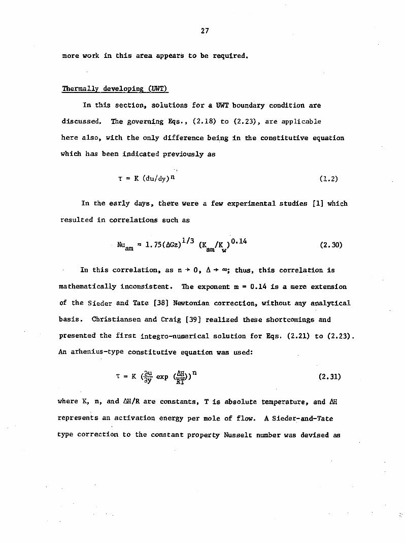
more work in this area appears to be required.
Thermally developing (UWI)
In this section, solutions for a UWT boundary condition are
discussed. The governing Eqs., (2.18) to (2.23), are applicable
here also, with the only difference being in the constitutive equation
which has been indicated previously as
T = K (du/dy)n (1.2)
In the early days, there were a few experimental studies [1] which
resulted in correlations such as
Nu „ = 1.75(AGz)l/3 (K /K )°* (2.30) am am w
In this correlation, as n -»• 0, A + thus, this correlation is
mathematically inconsistent. The exponent m = 0.14 is a mere extension
of the Sieder and Tate [38] Newtonian correction, without any analytical
basis. Christiansen and Craig [39] realized these shortcomings and
presented the first integro-numerical solution for Eqs. (2.21) to (2.23).
An arhenius-type constitutive equation was used:
T = K exp (A))" (2.31)
where K, n, and AH/R are constants, T is absolute temperature, and AH
represents an activation energy per mole of flow. A Sieder-and-Tate
type correction to the constant property Nusselt number was devised as

28
= exp (— - )) •R T
0.14 (2.32)
am
Christiansen and Craig have done elaborate calculations to show
that their correction gives better predictions than (K /K am w
Normally, near the tube inlet, constant property and variable consistency
Nusselt numbers are expected to be approximately equal. An increment in
the Nusselt number due to consistency variation is observed some
distance downstream from the tube inlet. In contrast, the Christiansen
and Craig solution results in exorbitantly high Nusselt numbers near
the tube inlet. Christiansen et al. [40] have extended the Christiansen
and Craig solution to the cooling of pseudoplastic fluids.
Forrest and Wilkinson [41] studied the effect of viscous dissipation
and internal heat generation. The K-t relation they used is
A substantial effect of consistency variation was demonstrated. To
account for viscous dissipation, the Brinkman number for pseudoplastic
fluid is defined as
It was shown that Br of the order of 10 can reverse the heat transfer
from heating to cooling. However, for laminar flow with small "u, Br will
rarely exceed a value of 0.001, and, hence, viscous dissipation can be
neglected for most fluids; but, if the fluid is highly viscous (high K ),
a substantial viscous dissipation can exist.
Kwant et al. [42] have utilized an approximate integral procedure
K - (1 + (2.33)
o (2.34)
o

29
as well as the Crank-Nicolson numerical scheme to solve Eqs. (2.18) to
(2.20). An exponential K-t relation was used in the calculation:
K = exp (-b(t-t )) (2.35)
Predictions for various n were correlated in terms of the ratio of velocity
gradients near the wall at the tube exit as
Nu, /Nu = 1 + 0.271 In * + 0.023(lné ) (2.36) Im cp e e
where (f) =((9u/9y) /(9u/8y) ) e w cp,w e
Popovska and Wilkinson [43] have also developed a numerical solution.
The K-t relation they used in their analysis is
K(t) = exp (A + Bt + Ct +••••) (2.37)
They have concluded that Eq. (2.30) gives good predictions in the entrance
region for all engineering calculations.
From the preceding discussion it is seen that there are numerous
publications in this area, and sound analytical bases exist to predict
heat transfer coefficients for the UWT boundary condition.
Thermally developing (UHF)
There are comparatively few studies in this area. Mizushina et al.
[31] have also studied thermally developing flows. The K-t relation they
used is given in Eq. (2.29). Their predictions for entrance region are
correlated as

30
Nu = 1.41 Al/3 Gz 1/3 (K/K jO.lO/nO* w
(2.38)
A fully developed correlation, Eq. (2.28) suggested by Mizushina et
al. has been already discussed. Thus, Mizushina et al. have suggested
two asymptotic equations to correlate predictions.
Cochrane [30] has utilized the Crank-Nicolson scheme to solve Eqs.
(2.18) to (2.20). The viscous dissipation was also included in the
energy equation, the effect of which was demonstrated to be insignificant.
The T-t relation he used is given in Eq. (2.31). For n = 1.0, 0.75,
and 0.5 predictions are obtained for AH/RT = 5 and 10. Thus, the predic
tions were not extensive enough to allow the development of a generalized
correlation. Cochrane's predictions for n = 0.5 are plotted in Fig. 2.5.
A peculiar maximum Nusselt number is seen in his solution. No
explanation is given for this phenomenon.
Equation (2.31) has its inherent weakness. For most fluids it is.
very difficult to know AH, the activation energy, unless the correct
chemical composition of the fluid is known. This equation can be
looked upon as
This is an exponential form of K(t), and if n is constant, this equation
is useful; however, for most pseudoplastic fluids, n is generally a
function of the temperature, and it is difficult to use Eq. (2.39).
These limitations of the constitutive equation notwithstanding, Cochrane
T = K(t) (3u/9y)* (2.39)
where K(t) = K exp (n AH/RT)
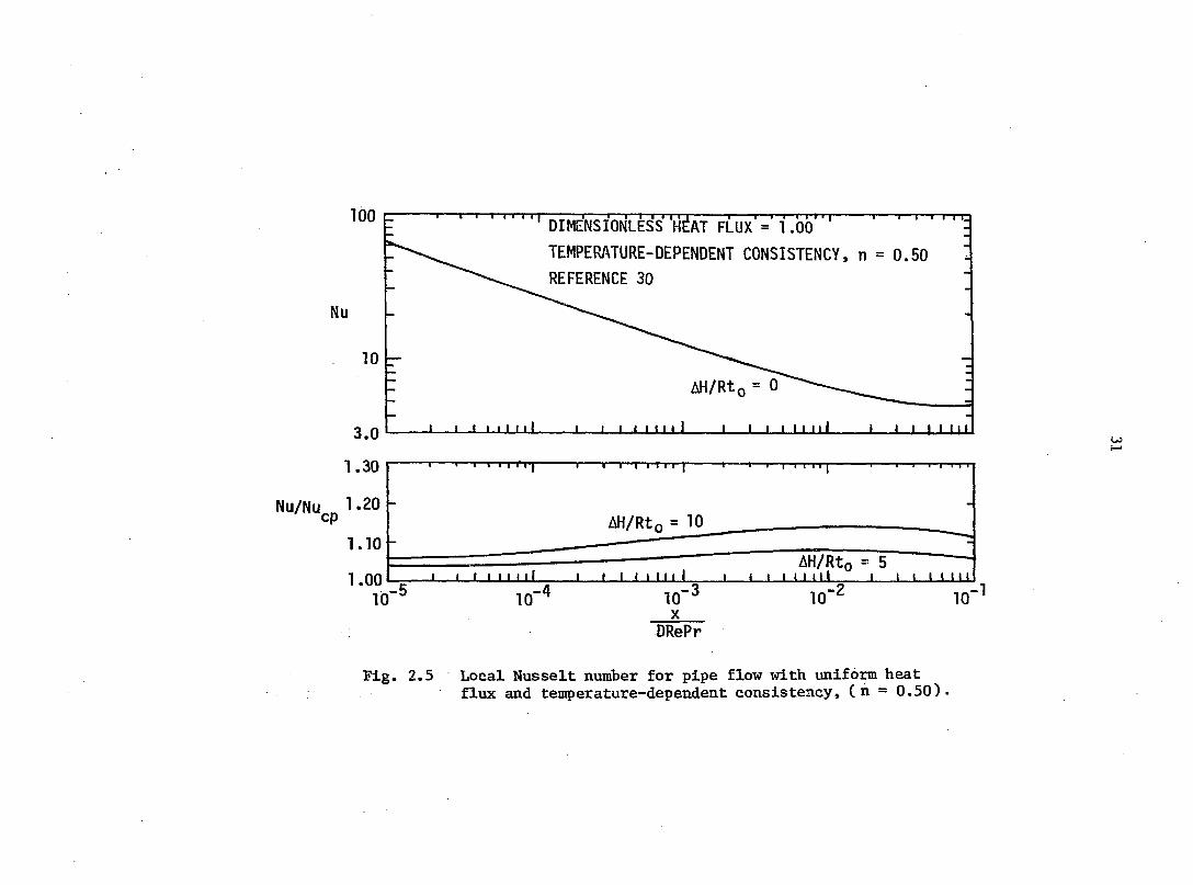
100 r
TEMPERATURE-DEPENDENT CONSISTENCY, n = 0.50 REFERENCE 30
Nu
3.0
1.30 T I I I 1 frj T r T I i I I I I I M I M I
Nu/Nu ^ 1.20 AH/Rto = TO
1.10 -
1.00
X DRePr
Fig. 2.5 Local Nusselt number for pipe flow with uniform heat flux and temperature-dependent consistency, (n = 0.50).

32
ha«; provided an escelleit foundation for future work.
Forrest and Wilkinson [44] have also developed an integro-numerical
solution to study, in particular, the effect of viscous dissipation and
internal heat generation. For a single value of wall heat flux» and
for n = 0.5, predictions were obtained for various values of viscous
dissipation and internal heat generation. A substantial effect of viscous
dissipation was found at Br = 10.0. The K-t relation they used is gi\«an
in Eq. (2.33). Mahalingam et al. [45] also published an integro-
numerical solution to the energy equation. The K-t relation they used
is given by
K = a exp (-bt) (2.AO)
The solution was used to compute tube wall temperatures, which were
compared with the authors' experimental results. A variation of the
order of 15 to 20 percent was noticed. The predictions are not given In
terms of n and, hence, are difficult to compare with other available
solutions.
From the preceding discussion, it is seen that with variable K,
only two predictions are available for n = 0.5 and 0.75. More
predictions with variable K to cover a wider range of heat fluxes are
needed for such intermediate values of n. There is also a need to
establish a generalized correlation to correlate the predictions.

33
Thermally and hydrodynamically developing
In this case, Eqs. (2,18) to (2.20) need to be solved simultaneously.
Korayem [29] and others [46,47] developed a solution for a UWT boundary
condition while Bader et al. [48] developed a solution for a UHF boundary
condition. Most of the pseudoplastic fluids are highly viscous and have
Pr » 5, thus, thermally developing solutions give adequately accurate
predictions. Thus, there seems to be no need for further work in this
area.
Conclusion
From the preceding discussion it is seen that a sound analytical
basis is available to predict heat transfer coefficients for a UWT.
However, for a UHF, for the entire thermal length, more predictions
are needed over a wider range of heat fluxes, i.e., a wider range of
K/K . To facilitate the work of a design engineer, a generalized
correlation needs to be established.
Scope for Further Work and Problem Definition
The preceding review of literature Indicates the need for further
work in the following areas:
1) For Newtonian fluids, more predictions are needed to clarify
the discrepancy between Yang's [32] and Shannon and DePew's [34] predictions
in the entrance region for a UHF boundary condition. For completeness,
predictions are also needed in the fully developed region.

34
2) For pseudoplastic fluids, a sound analytical basis exists to
predict heat transfer coefficients for the UÎ-JT boundary condition.
However, for a UHF boundary condition, more predictions are needed with
variable K for both developing and thermally developing regions. This
is particularly true for intermediate values of n, e.g., n = 0.75, 0.5.
The predictions are also needed over a wider range of heat flux (wider
range of K/K ). There is also a need for a generalized correlation over
a wide range of n and heat fluxes.
In addition to these areas, the following comments can be made
about some of the deficiencies in presently available analytical
solutions:
1) Various investigators use different forms of K-t or Ji-t, and
this makes it difficult to compare their predictions. The inadequacy
of Cochrane's [30] T-t relation, Eq. (2.31), has been already shown
(Eq. 2.39). The literature [45] shows that most of the viscous pseudo-
plastic fluids exhibit the K-t relation given in Eq. (2.40). This
exponential relationship is independent of n; hence, even if n is a
function of temperature over a certain range, Eq. (2.40) can be used.
Thus, a pseudoplastic analysis needs to be done for this K-t form.
2) All of the preceding solutions have used implicit numerical
schemes. Very recently Fletcher [49] has developed a direct, simple,
explicit numerical scheme using a stable Dufort-Frankel [50] method.
This non-iterative method is economical of computer time, and has
been used effectively to solve heat transfer problems by Fletcher and
Nelson [51,52] and by Hong and Bergles [53, 54, 55]. It is desirable

35
to develop such a scheme to predict heat transfer in pseudoplastic
fluids.
3) Most of the correlations for fully developed Newtonian or
pseudoplastic fluids are of the form as shown in Eq. (2.16) or Eq.
(2.28). For UHF this involves iteration for an unknown wall temperature
t and ]i . A direct, non-iterative equation would be welcomed by the
designer.
From this discussion, a specification of the analysis to be performed
is obtained as follows:
To devise an explicit numerical scheme to solve the problem of heat
transfer in steady laminar flow of a-pseudoplastic fluid inside a circular
tube and, for completeness, the Newtonian case is also to be considered.
The fluid consistency index, K, and density, p, are to be considered
temperature-dependent; however, the free convection effects can be
assumed to be negligible. All other fluid properties, such as k, c , and
n, are independent of temperature. The inertia and viscous dissipation
terms are to be retained in the momentum and energy equation, respectively.
The K-t relation applicable to most industrial fluids
K = a exp (-bt) (2.40)
where a and b are constants, is to be used. The predictions are to be
obtained for n = 1.0, 0.75, 0.50, and 0.25 for thermally developing flow
inside a tube subjected to a UHF boundary condition, and presented in
the form
Nu = f(Nu p, X+, n) (2.41)

36
CHAPTER III. NUMERICAL ANALYSIS
Introduction
After reviewing the literature, as summarized in the previous
chapter, it was decided to develop an explicit numerical scheme to solve
the problem of thermally developing heat transfer to the in-tube flow of
pseudoplastic fluids with temperature-dependent properties. In this
chapter, this scheme is described in detail. The coupled momentum and
energy equations are solved explicitly. The method and the computer
code developed can handle constant wall heat flux and constant wall
temperature boundary conditions.
Problem Formulation
Statement of the problem
The problem considered here is a steady laminar flow of a pseudo-
plastic fluid inside a circular tube. The tube is subjected to a
uniform wall heat flux boundary condition. At the inlet of the heated
tube (x = 0), the fluid velocity profile is fully developed and the
temperature profile is uniform. The fluid thermophysical properties
can either be dependent or independent of temperature; however,
buoyancy (free convection) effects are assumed to be negligible. The
problem involves determining the temperature profile development and the
variation in heat transfer coefficient along the axis.
In the present analysis, K and p are assumed to be temperature-
dependent, while k, Cp, and n are assumed to be constant. However, as
mentioned in the previous chapter, for viscous pseudoplastic

37
and Newtonian fluids, the K or y variation is of primary importance, and
the free convection effects arising due to p variation are insignificant.
Hence, the buoyant term in the momentum equation is neglected. As free
convection is neglected, the governing equations in the present
problem are two-dimensional and axisymmetric. The results are thus
independent of the geometric orientation of the tube.
The influence of pseudoplasticity on the fully developed velocity
profile is shown in Fig. 3.1. The Newtonian fluid (n = 1.0) has a
parabolic velocity profile. As n decreases, the fluid velocity profile
becomes flatter and flatter, generating sharp velocity gradients near
the wall and, fr'nally, for n = 0, a slug profile is observed. A similar
behavior is observed for the temperature profile. Considering the
physics of the problem, boundary layer approximations are used here which
state that the second derivatives in the stream-wise direction,
3 /3x , are negligible compared to those in the radial direction,
2 2 3 /8r , and the entire momentum equation for the radial direction can
be dropped.
In the present problem, the fluid velocity is fully developed at
the onset of heating; hence, at the inlet, v = 0. However, due to
property variations the fluid velocity profile will undergo changes.
Most of the previous analyses have assumed that these changes are
negligible (3u/3x =0, v = 0). For the fluids having strong temperature-
dependent K or y, 3u/3x may be significant and v # 0. It was thus
decided to retain all inertia terms in the momentum equation, and retain
the convective terms in the energy equation.

38
->•
->i
>1
»
??%?????????????????????? ? ?????? ???????? n = 0.0 n = 0.25 n = 1.0
Fig. 3.1 Laminar velocity profiles for pseudoplastic fluids.

39
For the viscous pseudoplastic fluids, the viscous dissipation
term may be significant [41,44]. However, Cochrane [30] and others
[31,45] have found that the term has little effect on the results.
Due to lack of clearcut guidelines, this term is retained in the
present analysis.
Governing equations
In formulating the equations, the following assumptions are
made:
1) Steady, axisymmetric flow
2) Axial conduction is neglected
3) Free convection effects are negligible
4) Usual boundary layer approximations are valid
5) Fluid properties K and p are temperature-dependent, while
k, Cp, and n are temperature-independent.
With these assumptions, the general governing equations in
cylindrical coordinates reduce to
momentum
(3.1)
energy
(3.2)

40
continuity
|_ (pur) + (pvr) = 0 (3.3)
In these equations T = K(3u/3y)" with (n 5 1)
and = K(9u/3y)""
The global continuity equation is also applicable:
J* pudA = constant (3.4) A
Far away from the tube inlet, fully developed velocity and
temperature profiles exist. In this region v = 0, 0, and
"ix ~ governing equations are then
momentum
- 3 + i 37 (ft) ' 0 ».5)
energy
continuity
§5 = 0 (3.7)
The boundary conditions for this problem are
For the velocity profile;
u(x,o) = 0, v(x,o) = 0, (9u/9y) = 0

41
For the temperature profile:
3y w I I
The initial conditions are
u(o,y) = u(y)
t(o,y) = t
P(O) = PG
Thus, there are four equations, (3.1) to (3.4), and four unknowns,
u, V, t, and p, and there are sufficient boundary and initial conditions.
Therefore, this problem is mathematically well posed.
Non-dimensionalized governing equations
The governing equations were non-dimensionalized. The list of
standard non-dimensional parameters is given in the list of symbols.
The resulting non-dimensional equations are
momentum
(3.8a)
where

42
energy
continuity
• »a (#)'
(W + 1^ (0VR) = 0 (3.10)
global continuity
ft m = y pUdA = constant (3.11)
A
The non-dimensional boundary and initial conditions are
U(X,0) = 0 , V(X,0) = 0
(||) = 0 , 0(0,Y) - U(Y) C
T(0,Y) = T(Y) , P(0) =
Finite-Difference Formulation
Dufort-Frankel method
Figure 3.2 shows the finite difference grid used in the present
analysis. An ordinary second-order explicit, central difference at
point (i,j) is

43
N N-1 N-2
I j-hl
j-1
I 1 2 1
CENTERLINE
+ Ay
Av" AX
Ù x' à +
X
12 3 4 -i-1 i i+1 WALL
Fig. 3.2 The finite-difference grid.

44
- 2 U + U - 2U (-5- ) = i»i»j 4. nfAY Z (3.12) 9Y AY
This formulation is found to be unstable. In the Dufort-Frankel method,
i+1 i i-1 i the term is replaced by averaging . This averaging
is a special feature of the Dufort-Frankel method [50], which considerably
enhances the stability of this explicit scheme. With this averaging
Eq. (3.12) is modified to
(|-4) = i,j+l i.j-1 i+l,j—1-1,j + o(Ay2, (3.13) i,j Ay2
This equation is rewritten as
"i+l.j - "1,1+1 + "l,j-l - "i-l.j - ».U)
It is seen that in this finite-difference formulation (Eq. (3.14)),
U . . c a n b e s o l v e d e x p l i c i t l y i n t e r m s o f k n o w n v a r i a b l e s a t t h e 1+1,J
previous two streamwise steps, namely i and i-1.
Apparent viscosity formulation
The apparent viscosity for pseudoplastic fluids is
K (|H)"-1 (1.3) ^ By
The finite-difference formulation for Eq. (3.8a) is
It is seen from Eqs. (1.3) and (3.15) that as (8U/9Y) j ->• o
y . . Thus, at the tube centerline and in the region very close â, 1, J
to it, p . . will be of an unrealistically high magnitude. To overcome ® ^ » J

45
this singularity, the viscosity is computed from the wall, along the
radius, up to the edge of the boundary layer, i.e., up to a point
where
U_ < 0.995 (3.16)
All the points laying in between the edge of the boundary layer and the
tube centerline, are assigned the same y . . value, as that on the a,i,j
edge of the boundary layer. Later, it will be seen from the results
of the numerical analysis that this approximation does not affect the
accuracy of the final predictions.
Finite-difference equations
The Dufort-Frankel finite-difference formulations and also the
standard ordinary explicit formulations of non-dimensional momentum,
energy and continuity equations are given in Appendix A.
Consistency, Stability, and Convergence of the Numerical Solution
Lax's equivalence theorem [56] states that for a well-posed initial
value problem and its finite-difference approximation, consistency and
stability are necessary and sufficient conditions for convergence. This
criterion is valid for linear partial difference equations. However,
even in the case of non-linear partial differential equations, this
criterion was found to hold fairly well, even though, Lax'a theorem has

46
never been proven for non-linear partial differential equations.
Consistency
Consistency deals with the degree to which the finite-difference
equations approximate the partial differential equation. The difference
between the two is called truncation error. A finite-difference
representation of a partial differential equation is said to be
consistent if the truncation error vanishes as the mesh is refined,
i.e., Lim. mesh 0,T.E. 0.
Consistency is generally studied by expanding the dependent
variables in a Taylor series and then estimating the truncation error.
Generally, the smaller the truncation error, the faster is the
convergence of the numerical scheme [56]. In the standard explicit
s cheme
where 0(AY) represents truncation error of the order AY. In the Dufort-
Frankel scheme.
(3.17)
= + 0(AY) AY
U - U (—) = '3+1 i.j-1
3Y 2AY (3.18)
= i>.1-n" 'j-l+0(AY)2
2AY
where 0(AY)2 represents truncation error of the order AY , which is

47
smaller than that noted for the standard ordinary explicit scheme.
The finite-difference approximation of the second derivative by Dufort-
Frankel scheme is
(—) i.i+1 " "i+lJ " Vl,.i "i.j-1 8y2 i,j " AY2
(3.19) 2 2
+ 0(AY2) + 0(UI) ( ) 3x2 Y2
The truncation error here is
2 0( ) + 0(AY2) Ay2
Thus, this formulation is mathematically consistent only if AX
goes to zero faster than AY. This requirement, will severely restrict
the step size in the streamwise direction. Fortunately, the entire
term consists of O u/SX )(AX/AY)2 and for boundary layer flows, 92u/3x2
is negligibly small as compared to other terms in the momentum equation.
Therefore, even for (AX/AY) - 1, Eq. (3.19) satisfies the consistency
requirement. The complete consistency analyses of momentum and energy
equations are given in Appendix B (Eqs. (A.l) and (A.2)).
Stability
Tlie essence of stability in obtaining the solution is that the
sequence of numerical procedures must be such that errors from any
source (round-off, truncation error, etc.) are not permitted to be
amplified and swamp the solution, i.e., errors from any source must be
damped as the calculations proceed from step to step. Mathematically,

48
this is expressed as: the error at the nth level should not grow when
the computation is completed for the solution at the n+1 level.
O'Brien et al. [57] have used Von Neumann's criterion to compute
stability of linear partial differential equations. This method has
been found to give fairly good results even for the non-linear partial
differential equations. In this method, local error is assumed to be
of the form
g = gOK eB? (3.20) i.J
If D represents the exact solution of the partial differential equation
and D+d' represents the solution of its finite-difference approximation,
then D+Ô' must also satisfy the partial differential equation. The
coefficients of the derivative terms are assumed locally constant or
error free. This is a simplification and gives rise to a "local"
stability criterion, but if the requirement is checked at each grid
point, then it is reasoned that an instability could not originate.
The condition for the error not to grow is
be reduced to
''i+i.j
Si.j < 1, which can
e < 1 (3.21)
For the ordinary explicit method, a maximum allowable step size (AY) is
found to be
(AX) max,j-l,N
i,j + j+1 ( a,i,j" a,i, j +1 ) +
U,,AY_
">1,3 "j "i.j
49
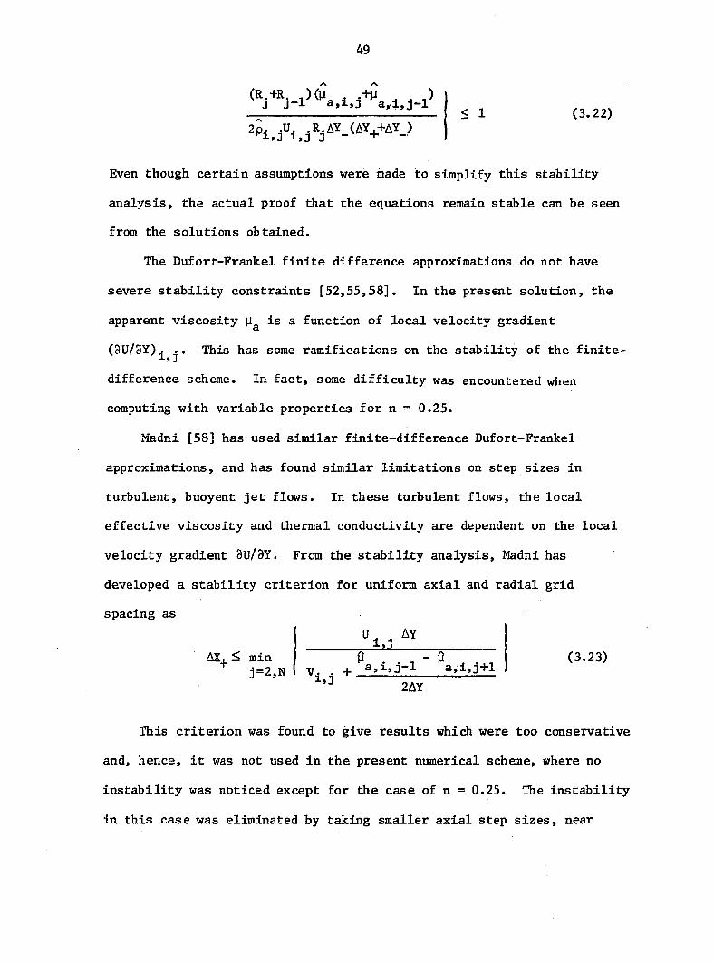
(3.22)
Even though certain assumptions were made to simplify this stability
analysis, the actual proof that the equations remain stable can be seen
from the solutions obtained.
The Dufort-Frankel finite difference approximations do not have
severe stability constraints [52,55,58]. In the present solution, the
apparent viscosity is a function of local velocity gradient
(3U/3Y) j •• This has some ramifications on the stability of the finite-J
difference scheme. In fact, some difficulty was encountered when
computing with variable properties for n = 0.25.
Madni [58] has used similar finite-difference Dufort-Frankel
approximations, and has found similar limitations on step sizes in
turbulent, buoyant jet flows. In these turbulent flows, the local
effective viscosity and thermal conductivity are dependent on the local
velocity gradient 3U/3Y. From the stability analysis, Madni has
developed a stability criterion for uniform axial and radial grid
spacing as
This criterion was found to give results which were too conservative
and, hence, it was not used in the present numerical scheme, where no
instability was noticed except for the case of n = 0.25. The instability
in this case was eliminated by taking smaller axial step sizes, near
AX <
U . . AY i»-l
(3.23)

50
the tube inlet of the order of (1/6) of the tube radius. This step
size was much larger than that obtained from the criterion suggested by
Madni.
In the present analysis, for n = 0.5, excellent results were
obtained by taking axial step sizes equal to almost half of the tube
radius at the tube entrance; further downstream the step sizes were
increased to be equal to the tube radius. Somewhat smaller axial steps,
of the order of one quarter of the tube radius at the tube entrance were
employed for the variable property computation.
Method of Solution
Grid spacing in the radial direction
One. of the major decisions to be made was the selection of the
number of grid points along the radial direction in the tube. A simple
procedure was followed to estimate an appropriate number of grid points.
A straight-line fit was used to estimate the velocity gradient at the
wall
A third-degree polynom: .;?. fit was also used to calculate the
velocity gradient at the wall. The four points near the wall were used
to do this as follows:
#). = TSA) + (PSB) + (PSC) ; (3.23)
+ (PSD)

51
where
2 PSB = 1 + D™ + DYM
AY_ DYM w
PSC = -1 + DYM + DYM
AY (1+DYM) DYM3
PSD = AY (l+DYM+DYM ) DYM
PSA = -(PSB 4- PSC + PSD)
and DYM = AY /AY _ (3.26)
It was found that for n = 1 to 0.5, the uniform grid spacing
(DYM = 1) in the radial direction gave excellent results. (This was
verified by using DYM = 1.05 and 1.10; no significant difference in the
final predictions was noticed). However, for n = 0.25, a nonuniform grid
spacing (DYM = 1.05) was found to give sufficient accuracy. In all the
numerical computations, the radial grid spacing was refined until the
velocity gradients at the wall, calculated by linear fit and polynomial
fit, agreed to within 0.5 percent.
Numerical procedure
In the Dufort-Frankel finite-difference equation, the unknown
variable at the i+l,j level is written in terms of known variables at
the previous two streamwise (axial) steps, namely i and i-1. In a
similar fashion, the equations of momentum, energy and continuity are

52
written explicitly and solved for the unknown values at streamwise step
i+1 in terms of the previous streamwise steps (see Appendix A). Once
all variables at streamwise step i+1 are known, they can be utilized
to evaluate unknowns at streamwise step i+2. Thus, a "marching
procedure" along the streamwise direction is followed. A flow chart
of the numerical marching scheme used here is given in Fig. 3.3.
It should be noted here that the Dufort-Frankel method is a three-
level method which utilizes information at the i and i-1 levels to calcu
late the variable at the i+1 level. At the inlet of the tube (x=0) infor
mation is known only at one station, i=l, and, hence, this three-level
method cannot be used. In order to overcome this difficulty, for the first
few initial steps (usually about the first 10 steps, near the tube inlet)
a standard ordinary explicit method which requires information only from
the previous step is used. The initial stability requirement for the
ordinary explicit method allows larger initial steps, AX, in the axial
direction; however, as the calculations progress along the axial
direction, the stability requirement for the ordinary explicit scheme
demands smaller and smaller axial steps. Therefore, an ordinary explicit
scheme is used only for the first few steps and then the Dufort-Frankel
method takes over. In general, it is desirable to use the largest
possible Ax, as this means fewer steps to cover the flow field and,
hence, less computer time.
Once the Dufort-Frankel finite-difference equations take over, the
step size for these equations is chosen as a constant multiple of the
boundary layer thickness. This axial step size is increased progressively

53
JiO_ YES
YES
START
CALCULATE AX
OUTPUT
READ IN DATA AND INITIALIZE
END? STOP
CALCULATE P^+^
CALCULATE V.
CALCULATE T.+^ j
CALCULATE U.+^ ^j
CALCULATE K-
CALCULATE j
CALCULATE, Nu, X , Gz, Re^
Re, Pr , Pr, etc.
1+1. j
Fig. 3.3 A flow chart of the computer program.

54
as the calculation marches forward in the axial direction. The axial step
size is increased until it is equal to the radius of the circular tube.
This point is reached noirmally near the fully developed region
(V = 0, = 0).
To start with, the pressure at location i+1, is computed
from the integral form of the global continuity equation. Details of
this calculation are shown in Appendix C. Now, the U . . at all j's are
computed from the momentum equation, (A.l) or (A.4), as all variables
at previous strearawise levels are known. After this, the finite
difference form of the energy equation, (A.2) or (A.5), is solved to
ob tain the temperature T _j_2 j all j's. The fluid density is then
computed at all j's, and substituted in the continuity equation, (A.3)
or (A.6), to compute V , at all j's. This completes one set of i+1, J
calculations.
After this, all i+1 variables are assigned the value of these
variables at the i location. The previous i location becomes the i-1
location. At this new i location, K. • and u . are calculated. All a,i,j
variables are again known at i and i-1 locations, and another forward
step is marched in an axial direction by repeating the same procedure.
It should be noted here that each variable is calculated explicitly
at each location. No iterations or simultaneous solutions are necessary;
this saves considerable computer time.
Calculations of viscosities arid flow parameters
The viscosity of pseudoplastic fluids is defined in two ways. First,
the apparent viscosity is

55
Pa = K (1.3)
This viscosity is used in the numerical computational procedure. The
other viscosity is called the effective viscosity. This is defined as
the viscosity that would have existed at the wall if the fluid would
have been Newtonian.
For Newtonian fluids T = [y (—)]„ (3.27) 9y Newt
and, hence, „ 9uxn T
= — (3.28)
This viscosity definition has been used by Skelland [1] and others
[59,60].
From the definitions of effective and apparent viscosities,
Reynolds numbers were computed as
Re = and Re = — (3.29) V'eff
Similarly Pr and Pr were computed. The effective Reynolds number Re
gives the following well-known relation for the fully developed friction
factor for laminar flow of Newtonian fluids
f - H ( 3 . 3 0 )
Based on these parameters, a non-dimensional length X is calculated as
X" = 2(x/D)/RePr (3.31)

56
and the Graetz number is
Gz = TT/2X''' (3.32)
Calculation of heat transfer results
The major aim of the analysis was to predict heat transfer
coefficients and Nusselt numbers along the tube length. However, before
computing these parameters the following procedure was followed to
ensure the accuracy of the numerical computation
1) At each axial location the heat balance of the heat supplied
along the tube wall, Q , and the heat absorbed by fluid, Q , were
assessed:
Qg = /" dQg = dx (3.33) o o
Qa = S " *:o) (3-34)
In no instance, did the difference between the two exceed 0.3 percent.
In most of the calculations, this difference never exceeded 0.1 percent.
2) At each axial location, the wall temperature gradient (3t/3r)
was computed by linear and polynomial fit as shown for (8u/3r) in
Eqs. (3.24) and (3.25), and then wall heat flux was computed as
w
For a UHF boundary condition, the wall heat flux q" was known, and,
therefore, in all numerical computations, it could be verified that the

57
difference between the q"__ and [q" ] . did not exceed 0.20 w w prediction
percent. In most of the calculations, this difference never exceeded
0.01 percent.
At station x, at which the output was desired, knowing velocity and
temperature profiles, the bulk temperature was computed as
w /
w tur dr
o
/ " ur dr
t, = o (3.36) D
The local heat transfer coefficient is defined as
(3.37)
and, therefore,
" (A)
The local Nusselt number based on tube diameter, D, is
Nu = - (3.39)
Substituting Eq. (3.38) into Eq. (3.39) yields
Computer code
A computer code which was developed to solve this problem is given
in Appendix D.. This code was developed from the computer code, developed
by Nelson [51] for the Newtonian heat transfer. A considerable

58
modification of this code was done to utilize it for non-Newtonian flow
and heat transfer. Some of the features of this code are as follows;
1) Two most commonly encountered boundary conditions in heat
transfer studies, namely, a constant wall heat flux and a constant wall
temperature can be used.
2) The fluid density, specific heat, thermal conductivity, coef
ficient of thermal expansion, flow behavior index, and the consistency
index, are incorporated as temperature-dependent function sub-programs.
This facilitates use of the main program for either constant fluid
property conditions or variable fluid property conditions, where any
specified fluid property-temperature relationship can be used. The free
convection effects are neglected in the governing equations as they are
estimated to be small.
3) The program can handle thermally developing or thermally and
hydrodynamically developing flows.
4) Provision is made in the program to handle either an isothermal
or a nonisothermal temperature profile at the entrance of the heated tube.
5) Provision is made in the program so that at the axial position,
at which the program stops, all the variables at that station are recorded
on a disc. Then, when it is desired to proceed further downstream, the
results of the last axial station from the previous calculation esn be
read from the disc, and computation from that axial station onwards can
be started.
6) With very little modification, the present numerical scheme can
be modified to compute heat transfer calculations for flow of pseudo-
plastic fluid over a flat plate.

59
CHAPTER IV. NUMERICAL RESULTS AND DISCUSSION
In this chapter, the predictions obtained from the numerical scheme
developed in Chapter III are discussed. These predictions are for the
flow of pseudoplastic fluid inside a circular tube subjected to a uniform
wall heat flux boundary condition. At the onset of heating, the fluid
velocity profile is fully developed and isothermal.
Constant Property Predictions
Heat transfer
The assumption of constant thermophysical properties is highly
restrictive, particularly with regard to K. For most pseudoplastic
fluids, with every 25-30°F change in temperature, K undergoes a change
of about 50 to 100 percent. However, constant property predictions
provide the basis for the comparison of the variable property
predictions. In the computer code developed, all the fluid properties
were incorporated as subroutines. For this analysis, constant values
were assigned to these subroutines.
In this analysis, the predictions for the local Nusselt numbers
were obtained for the entire thermal length, for n = 1.0, 0.75, 0.5 and
0.25. For the fully developed case, the temperature difference (t - t )
is constant and, hence, a constant asymptotic value of Nusselt number
is obtained.
Table 4.1 shows that the fully developed predictions of the
present analysis are in excellent agreement with the analytical

60
Table 4.1. Comparison of non-Newtonian Nusselt numbers for the fully developed region
n
Nu*
n Present Ref. 22-23 Eq. (4.1)
1.0 4.36 4.36 4.36
0.75 4.50 4.50 4.48
0.50 4.75 4.75 4.70
0.25 5.31 5.31 5.25
0.10 6.25 6.25 6.46
predictions of Seek and Eggink[22] and Grigull [23] which are correlated
by Eqs. (2.9) and (2.10) respectively. These two correlations give
identical results and account for the increase in Nusselt number due to
pseudoplasticity. However, these correlations are highly complex and,
therefore, Pigford [25] and Mzushina et al. [31] have suggested a
simple correlation
4.36 (4.1)
where A = (4.2)
4n
1/3 The non-Newtonian correction, A is simple and gives accurate results
within 1.1 percent, in the range of n = 1.0 to 0.25, and within 3.0
percent at n = 0.1 (see Table 4.1). It is important to note that as
n ->• 0, A-> 00and, hence, this correction is mathematically inconsistent.
However, since most engineering fluids have n > 0.25, Eqs. (4.1) and

61
(4.2) can be used for all engineering calculations. The excellent
agreement of the present predictions with these equations and previous
predictions demonstrates the success of the present explicit finite-
difference scheme.
Figures 4.1 to 4.4 are plots of local Nusselt numbers against
•f* dimensionless distance, X , for the entire thermal length, for n = 1.0,
0.75, 0.5 and 0.25 respectively. In these plots the present local
Nusselt number predictions are compared with available predictions
[8,9,11,16,30,31,44]. The excellent agreement with these predictions
further confirms the accuracy of the present explicit finite-difference
scheme.
For the case of n = 1.0 (Fig. 4.1), the present predictions and
those of other investigators [9,11,17] are lower than the predictions
of Kays [8]. This may be due to the large grid spacing used by Kays
in his computation.
Figure 4.5 is a composite plot of local Nusselt numbers against
for various values of n. It is distinctly seen that the effect of
pseudoplasticity is to increase heat transfer coefficients above the
Newtonian values. This increase is quite substantial at lower values
of n. To account for this effect, Mizushina et al. [31] have suggested
that the fully developed correction could be used. However, they
never established the validity of this correction in the thermal
entrance region.
The non-Newtonian correction, was applied to all of the
present data as indicated in Fig. 4.6. It is seen that throughout the

60.0
NEWTONIAN FLUID, n = 1
CONSTANT FLUID PROPERTIES
PRESENT RESULTS 10.0
O KAYS [8]
• WORS0E-SCHMIDT [9]
A BUTTERWORTH AND HAZEL [16]
• SIEGEL, SPARROW. AND HALLMAN [11]
2.0
Fig. 4.1 Comparison of present numerical solution with available predictions (n = 1) .

60.0
CONSTANT FLUID PROPERTIES
Nu
PRESENT RESULTS 10.0
O COCHRAN [30]
2 .0 2 3 1 1 4 2x10
Fig. 4.2 Comparison of present numerical solution with available prediction (n = 0.75).

60.0
CONSTANT FLUID PROPERTIES
^-PRESENT RESULTS\..^^^^
A MIZUSHINA et al. [31]^^ O FORREST AND WILKINSON [44] 10.0
2.0 2x10
Fig. 4.3 Comparison of present numerical solution with available predictions (n = 0.5).

60.0
CONSTANT FLUID PROPERTIES
10.0 O COCHRAN [30]
PRESENT RESULTS
2.01
10 2x10 10
Figure 4.4 Comparison of present numerical solution with available predictions (n = 0.25).

60.0
CONSTANT FLUID PROPERTIES
10.0
n =0.25 n = 0.50
2x10 ,+
Fig. 4.5 Results of the present numerical analysis for laminar in-tube flow of power law fluids.

60.0
CONSTANT FLUID PROPERTIES
1/3
10.0
an = 0.50 = 0.25
_ n = 1.0, NEWTONIAN
2.0 4 3 2
Fig. 4.6 Comparison of corrected Nusselt numbers for non-Newtonian flow predictions with Newtonian flow predictions.

68
entire thermal length this correction gives excellent results for
n = 0.75 and 0.50. However, for n = 0.25, this correction somewhat
over corrects (2-3 percent) in the early part of the entrance region
CX" < 2 X 10" ). In light of the fact that the non-Newtonian
correction employed is "approximate", the corrected Nusselt numbers
are in excellent agreement with the Newtonian predictions. This
confirms the validity of the non-Newtonian correction, to
account for an increment in heat transfer due to pseudoplasticity
throughout the entire thermal length. The tabulated predictions are
given in Appendix E.
Pressure drop
For the hydrodynamically developed, in-tube flow of pseudoplastic
fluids, it can be shown that [1]
(8%)* (4.3) dx D 4n D
For constant property flow, Eq. (4.3) will give a constant pressure
gradient dp/dx. A comparison of the predictions from Eq. (4.3) and
from the present numerical scheme is given in Table 4.2.
Table 4.2. Comparison of pressure gradients
n -» 1.0 0.75 0.5 0.25
dp/dx, numerical -0.046 -35.40 -11.92 -3.09
dp/dx, Eq. (4.3) -0.046 -35.38 -11.92 -3.07

69
There is a Ï 1 to 2 percent variation in the pressure gradient at
various axial grid cross-sections along the tube length. This slight
variation is simply due to finite-difference approximations, which
are inherent in the numerical calculations. The constant average
values of dp/dx are given in Table 4.2.
Most of the numerical studies calculate dp/dx while, most of the
experimental studies evaluate f, the friction factor. In Chapter III,
it was shown that for pseudoplastic fluids,
f = 16/Re (3.30)
Where Re is based on the defined in Eq. (3.28). A comparison
of the Fanning friction factor obtained from Eq. (3.30) and the
predictions from the numerical computation is given in Table 4.3.
Table 4.3, Comparison of Fanning friction factors
n ->• 1.0 0.75 0.50 0.25
Re ->• 284.2 8.3 24.6 13.6
f, numerical 0.056 1.931 0.650 1.185
f, Eq. (3.30) 0.056 1.928 0.650 1.182
It is seen that the f values are in excellent agreement with the
theoretical results, in accordance with the results given in Table 4.2.

70
ConclusIon
The present heat transfer predictions are in excellent agreement
with the available predictions. The pressure drop and friction factor
predictions are also in excellent agreement with the theoretical
predictions. This confirms the success of the present explicit
numerical scheme.
1/3 The non-Newtonian heat transfer correction, A ' , is also confirmed
for the entire thermal length.
Variable Property Predictions
Introduction
In this section, heat transfer predictions for pseudoplastic fluids
with variable properties are given. The constitutive equation for a
pseudoplastic fluid is
T = K( ) with (n < 1) (1.2)
For Newtonian fluids, n = 1, and K represents the viscosity, y.
Most of the power-law fluids are highly viscous in nature and exhibit a
strong temperature dependence for K, while n is normally a weak function
of temperature.
As mentioned earlier in Chapter III, in the present analysis the
following assumptions are made:
1) K and p are temperature-dependent, but the free convection
effects are negligible.
2) k, Cp, and n are temperature-independent. The assumption of

71
constant k, c , and n is not highly restrictive, since for many liquids
these properties are very weak functions of temperature.
3) The fluid has a fully developed, isothermal velocity profile
at the onset of heating.
The K-t relation used is
K = a exp (-bt) (2.40)
where a and b are constants. This log-linear relationship is found to
be valid for most pseudoplastic fluids [45]. Many Newtonian fluids
also exhibit this kind of temperature dependence of viscosity.
The p-t relation used here is
p = A1 + A2n + A3ri + A4ti (4.4)
where A1 to A4 are constants and n = (t-50.0)/50.
This relation holds for most aqueous solutions. It is important
to note that the free convection effects were neglected, as the density
variation is quite negligible as compared to the K variation. However,
density variation was accounted for in the convective and inertia terms
in the governing equations.
The objective of this analysis was to evaluate the effect of
variable K on the heat transfer coefficient for flow of a pseudoplastic
fluid inside a tube. For the uniform wall heat flux boundary condition,
predictions are to be obtained for various n values, for the entire
thermal length.

72
A parameter to account for variable consistency
Shannon and Depew [34] and Hong and Bergles [54,55] have done
analyses for fully developed heat transfer with Newtonian fluids. These
investigators have used "arhenius-relations" for y-t as
y = Wg exp (-Y(t-t )) (2.17)
where
Y = - — = constant (4.5) y dt
Hong and Bergles have defined a non-dimensional viscosity
parameter as yAT. This parameter is similar to gAT in the Grashof
number which accounts for density variation. For the constant wall
heat flux condition, AT is replaced by
q" D AT = (4.6)
and, hence, from Eqs. (4.5) and (4.6)
YIT = (-I (4.7)
It is important to note that until now this parameter was used
only for fully developed Newtonian heat transfer. In the present
analysis this concept is extended to pseudoplastic fluids, where in
Eqs. (4.5) and (4.7) y is replaced by K.
Since K = a exp (-bt)
Y = — ( ) = b = constant (4.8)

73
and
(4 9)
This parameter can be varied by either varying wall heat flux or by
selecting a fluid with different y.
Numerical variables
In the present analysis, variable property predictions were
obtained for n = 0.75 and n = 0,50 for the entire thermal length. For
a given pseudoplastic fluid, different values of yAT were obtained by
varying the wall heat flux, q" . The predictions were obtained for w
four different values of yAT which were sufficient for correlation.
The limiting case of a pseudoplastic fluid is a Newtonian fluid
(n = 1.0) and, therefore, for completeness, variable property
predictions were also obtained for the Newtonian case. For this case,
properties of highly viscous transformer oil are used. The transformer
oil has a strong temperature-dependent viscosity, which for the most
part can be described by an exponential function (Eq. 2.40). For this
Newtonian case, predictions were obtained for the entire thermal length
for two different values of yAT (two heat fluxes) .
The analytical procedure followed here was identical with the one
followed for constant property analysis, with the only difference being
that the appropriate K-t and p-t relations were incorporated in the
fluid property subroutines.
For the Newtonian case alone, with the variable |i assumption, an
additional analysis was made for the fully developed region. Simpson's

74
rule for numerical integration was used to solve the differential
equations occurring in this analysis. The predictions were obtained
for six different values of yAT, two of which were the same as used
in the Dufort-Frankel marching scheme. This duplication was done to
varify the fully developed Newtonian prediction for both schanes.
The details of this Newtonian fully developed analysis are given in
Appendix F.
Nusselt number results
The variable property local Nusselt number predictions, for
the entire thermal length and for various yAT values are
tabulated in Appendix G. Figures 4.7 and 4.9 are the plots
of local Nusselt numbers against dimensionless distances, X"*",
for n = 1.0, 0.75, and 0.5 respectively. In these plots,
continuous smooth curves were drawn through the predicted data
points; however, for clarity, the data points are not shown.
The Newtonian predictions, for the entire thermal length, for
yAT =2.35 and 3.77 and also the predictions from the special fully
developed analysis are shown in Fig. 4.7. The fully developed
predictions by both schemes for yAT = 2.35 and 3.77 are identical
(see Appendix F and G).
Figures 4.7 to 4.9 distinctly show that there is a substantial
increase in heat transfer coefficient when heating, due to temperature-
dependent properties. For the given wall heat flux (given yAT) the
increment in heat transfer is much more pronounced at n = 0.5 than
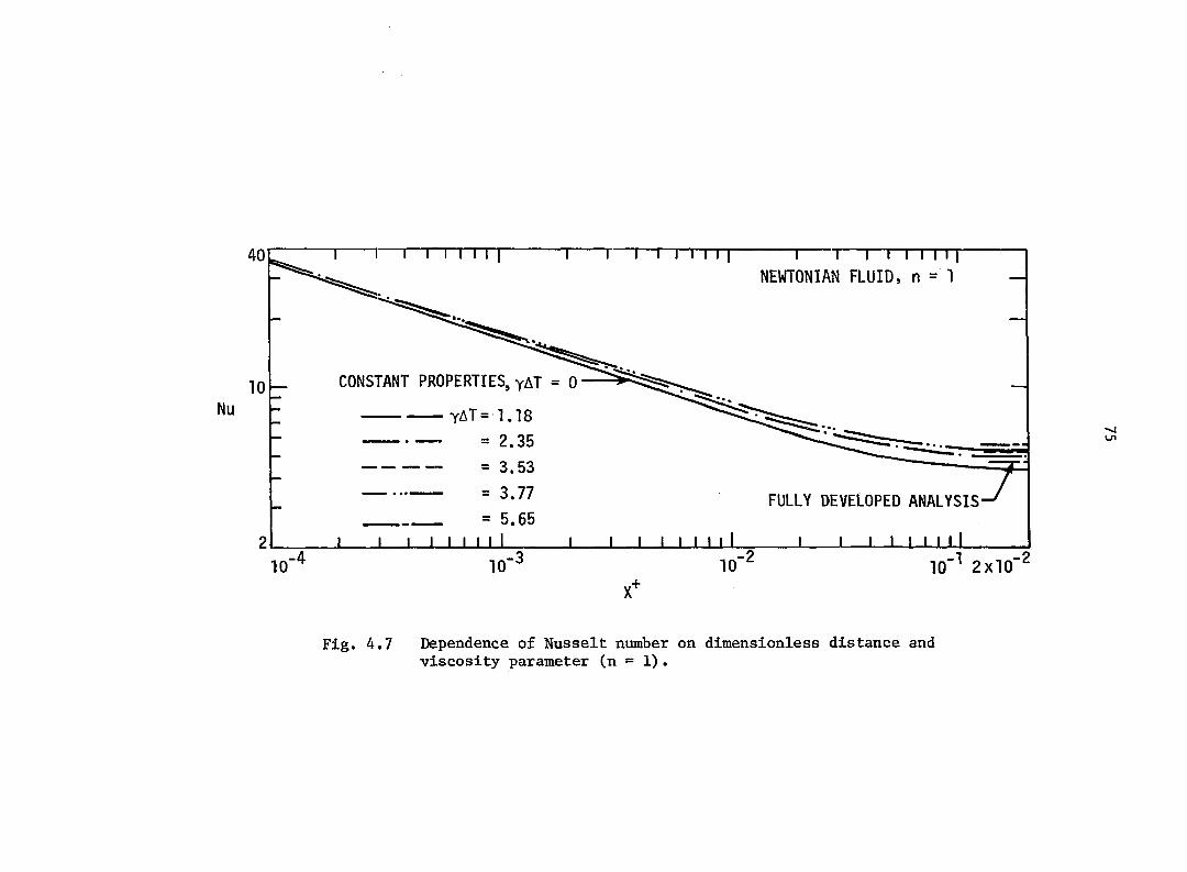
NEWTONIAN FLUID, n = 1
CONSTANT PROPERTIES, yAT
yAT =1.18 Nu
= 3.53
FULLY DEVELOPED ANALYSIS = 5.65
10"' 2x10 ,+
Fig. 4.7 Dependence of Nusselt number on dimensionless distance and viscosity parameter (n = 1).
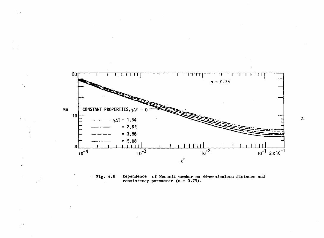
50
0.75
CONSTANT PROPERTIES,yAT = 0 10
yAT = 1.34 = 2 .62
= 3.86
= 5.08 3
2x10 ,+ X
Fig. 4.8 Dependence of Nusselt number on dimensionless distance and consistency parameter (n = 0.75).

60.0
0.5
CONSTANT FLUID PROPERTIES, yAT
YAT= 1.34
= 2.62
= 3.87
= 5.12
2.0 10 ' 2x10
,+
Fig. 4.9 Dependence of Nusselt number on dimensionless distance and consistency parameter (n = 0.5).

78
that at n = 1.0. As expected, the effect of variable properties is
greater in the fully developed region than in the thermal entrance
region.
This increase in heat transfer coefficient is mainly due to the
variation in temperature-dependent K for pseudoplastic fluids and
temperature-dependent JJ for Newtonian.fluids. In order to correlate
this effect, for each n at constant yAT and at several axial locations,
a ratio of variable property and corresponding constant property
Nusselt numbers, (Nu/Nu ) , was calculated and plotted against the cp %+
corresponding ratio (K/K ) . At the tube entrance, (K/K ) = 1.0.
As the fluid progresses downstream inside the tube, progressively higher
values of (K/K ) are observed. Thus, for a given wall heat flux, lower
values of (K/K ) exist in the thermal entrance region, and comparatively
higher values of (K/K ) exist in the fully developed region.
For n = 1, a logarithmic plot of (Nu/Nu p) against
is shown in Fig. 4.10; for clarity, the data points are not shown.
Similar plots of Nusselt number ratio for n = 0.75 and n = 0.5 (with
abscissa (K/K ) +) are shown in Figs. 4.11 and 4.12, respectively.
All of these plots have similar characteristics. These logarithmic
plots show that
1) For the Newtonian fluid in the entire thermal development
region (entrance as well as fully developed), a log-linear relationship
is observed. The slope of this straight line is 0.14 and therefore
(4-10)
where m = 0.14. These results are similar to those obtained by

FULLY DEVELOPED PREDICTIONS O yAT = 1.18
• = 2.35
B = 3.53
A = 4.00 A = 5.65
NEWTONIAN FLUID, n = 1
PREDICTIONS FOR THERMAL ENTRANCE LENGTH FOR yAT = 2.35 AND 3.77
J I L 8 9 10
Fig. 4.10 Dependence of Nusselt number ratio on viscosity ratio (n = 1) .

YAT= 1.34 = 2 .62
= 3.86
= 5.08
0.75
1 1 2 3 4 6 5
Fig. 4.11 Dependence of Nusselt number ratio on ratio of consistency indices (n = 0.75).

Nu
(""cp)
n = 0.5
YAT= 1.34
= 2.62
= 3.87
= 5.12
Fig. 4.12 Dependence of Nusselt number ratio on ratio of consistency indices (n = 0.5).

82
Yang [32] (see results and discussion in Appendix F for further details).
2) For n = 0.75 and 0.5, a log-linear relationship is observed
near the tube inlet (thermal entrance region). The slopes of these
straight lines are dependent on n. For n = 0.75 and 0.5, the m values
are 0.25 and 0.36, respectively.
3) For a given heat flux, at higher values of K/K , i.e., in the
fully developed region, an asymptotic value of the ordinate is observed
for n = 0.75 and 0.5. The value of this asymptotic ordinate is
4) For n = 0.75 and 0.5 and for a given yAT, the value of the
asymptote is a function of n.
5) For the given two values, the difference between
while for n = 1.0, there are no asymptotes.
Thus it is seen from Figs. 4.10 to 4.12 that in the entrance
region, the Nusselt number ratio is a function of n and K/I while in
the fully developed region the ratio is a function of n and yAT. This
can be mathematically summarized as
The functional relationship is quite complex, and it is difficult to
obtain a simple correlation. Therefore, an approximate correlation
is developed which is sufficiently accurate for design purposes.
The variable property predictions are tabulated in Appendix G.
asymptotic values of (Nu/Nu ) is larger at n = 0.5 than at n = 0.75,
= £Cn, YAI, (K/VJ cp ^
(4.11)

83
Development of a variable consistency correction
The consistency correction is devised in two steps: 1) thermal
entrance correction and 2) fully developed correction.
In the thermal entrance region, for a given n, a log-linear
relationship is observed between (Nu/Nu ) and (K/K ) _j_. The slope,
m, of these straight lines was found from Figs. 4.10 to 4.12. This is
tabulated in Table 4.4.
Table 4.4. Predictions of m in the thermal entrance length
n m
1.0
0.75
0.50
0.14
0.25
0.36
A linear regression analysis for these three points gives
m = 0.58 - 0.44n (4.12)
with a correlation coefficient of 0.999. Thus, for the thermal entrance
region, the local Nusselt number can be written in terms of the
corresponding constant property Nusselt number as
(Ku)jj+= (4.13)
As noted earlier, for the fully developed region, the predictions
were obtained for four different values of yAT at each of two values of

84
n, 0.75 and 0.5. For n = 1, the predictions were obtained for two
different values of yàT. However, for the Newtonian case alone an
independent fully developed analysis was done, in which predictions
were obtained for six different values of yAT. TVo of these
predictions have identical to those used in the Dufort-Frankel
numerical scheme. These fully developed predictions are tabulated in
Table 4.5
A plot of (Nu/Nu p) against yAT for n = 1.0, 0.75, and 0.5 is
shown in Fig. 4.13. Each of these three curves is correlated by
second-order polynomial.
For n = 1.0
(4.14)
(4.15)
(4.16)
(4.17)
The coefficients and are functions of n, A linear regression
analysis was used to correlate C, and C„ J- 2
(_Ny_) = 1.0 + 0.069yAT - 0.0033(yAT)2 N"cp ~
For n = 0.75
(- )oo = 1.0 + 0.0847yAT - 0.0051 (yAT) Nucp
For n = 0.50
(~ )„ = 1.0 + 0.0961yAT - 0.0067 (yAT) cp
The generalized form of Eqs. (4.14) to (4.16) is
( )oo = 1.0 + C (n)yAT - C2(n)(yAT)2

85
Table 4.5. Fully developed heat transfer predictions
n yAT (Nu/Nu p)„
1.0 0.0 ' 1 .00
1.18 1.08
2.35 1.14
3.53 1.20
3.77 1.21
4.00 1.23
5.65 1.28
0.75 0.0 1.00
1.34 1.11
2.62 1.18
3.86 1.25
5.08 1.30
0.50 0.0 1.00
1.34 1.12
2.62 1.21
3.87 1.27
5.12 1.32

.4
FULLY DEVELOPED NUMERICAL RESULTS
.3
. 2
CORRELATIONS, EQS. (4.14)-(4.16)
1.1
1 7 3 4 5 6 0 2 1
YAT ' i%r [^(^)]
Fig. 4.13 Dependence of Nusselt ratio on
87
C (n) = 0.12392 - 0.05420n (4.18)
and
CgCn) = 0.010133 - 0.0068n (4.19)
With this Eq. (4.17) is rewritten as
(4.20)
where
Ck= Ci(n)YAT - C2(n)(YAT)2
Equation (4.20) is a generalized correlation for the fully
developed region. For a given fluid, n and b are known, and for a
given heat flux, yAT is estimated; then, using Eq. (4.20, (Nu/Nu p)
can be estimated explicitly. All the available predictions for fully
developed flows of Newtonian and pseudoplastic fluids [31-34] are of
the form given in Eq. (4.10). For the constant wall heat flux boundary
condition, t and are unknown quantities, and iterations are
essential to evaluate Nu. The present proposed correlation (Eq. (4.20))
does not involve any iterations, and, therefore, it is highly useful
for design purposes. A plot of (Nu/Nu p) is shown in Fig. 4.14.
This plot demonstrates the validity of the proposed fully developed
correlation.
The value of yAT used in the present numerical scheme (yAT 5 8) is
sufficiently high to cover most of the pseudoplastic fluids and heat
duties encountered in practice. However, some sort of extension was
needed to cover extreme values of yAT. It is to be emphasized here

1,41 I I I I I I ~! I
o n = 1.0
, ,, Û n = 0.75 • n = 0.50 /EQ" (4.20)
'•2
0.0 0.02 0.06 0.10 0.14 0.16 0.20 0.24 0.28 0.30 0,32
Fig. 4.14 Dependence of Nusselt ratio on consistency correction factor Cj .

89
that the extension is needed only for the fully developed region, while
the results for the thermal entrance region are well established by the
present analysis, independent of yAT.
For the fully developed case, for a given n, the physics of the
present problem seems to indicate that with an increase in yAT there
should be an increase in (Nu/Nu ) . However, in the present correlation, cp
Eq. (4.20), the maximum value of (Nu/Nu ) occurs at
Thus, for yAT > (yAT) , Eq. (4.20) will give incorrect predictions. max
In order to overcome this difficulty, attempts were made to correlate
yAT and (Nu/Nu ) in such a fashion that all the coefficients in the
correlation should have positive values. Attempts were made to fit either
various polynomials or exponential forms, but all these attempts gave
much poorer correlations of the present numerical predictions. Some
attempts were made to extend the present correlation to higher values of
yAT, but these attempts are too speculative, and since no experimental
or numerical data are available for higher yAT values, it was not
possible to devise an extended correlation. The data of Bassett and
Welty [61] have yAT of the order of 20, but these data are restricted
to the entrance region and can be reduced by the present analysis.
More data are needed for such high yAT values in the fully developed
region to devise a meaningful correlation.
Cj (n) (4.21)
C2(n)
cp a>

90
Design procedure
The effect of two corrections, namely the thermal entrance
correction and the fully developed correction, is schematically shown
in Fig. 4.16. As seen from this figure, in the proposed correlation,
the thermal entrance region and the fully developed region are well
correlated, but the transition region from the thermal entrance to fully
developed section is slightly underprsdicted. There have been two
experimental studies [45,61] in this area. It will be shown later that
the present proposed correction gives excellent results when applied
to these experimental data sets, thus implying an Insignificant effect
of the overcorrection.
The problem still unresolved is how to estimate point "crit" in
Fig. 4.16, i.e., determination of a point up to which the thermal
entrance correction is applied and after which a fully developed
correction is applied. A simple procedure to determine ((K/K ) ,) w crit
is as follows :
For a given fluid, b and n are known and a wall heat flux q" is
also known. Using Eq. (4.20), (Nu/Nu ) is estimated; also using
Eq. (4.12), the thermal entrance correction exponent m is estimated.
Thus as shown in Fig. 4.15, the intersection of fully developed
correction and entrance region correction is a transition point "crit"
at which the (K/K ) +value is .
Thus,
( ) , = (C_)* (4.22) Nucp X+

EQ. (4.20)
[(K/r)x+]
( I J )
VARIABLE PROPERTY PREDICTIONS ABC (CONSTANT PROPERTY, n = 1.0)
CONSISTENCY CORRECTED PRDICTIONS
n, yaT
'YAT = 0
(K/Kv,)x+
Fig. 4.15 Schematic diagram of the consistency correction.

92
where
<=c"WVx+
and
C = ((K/' )x+>crit ' "•'/Vx+'crlt
In conclusion, pseudoplastic fluids having temperature-dependent
fluid properties exhibit substantially higher heat transfer coefficients
than Newtonian fluids. This increase is due to
1) Pseudoplasticity, which can be accounted for by applying
the non-Newtonian correction,
2) Variable consistency effects, which can be accounted for by
applying the (C )™ correction.
Summary and Conclusions
An explicit stable numerical scheme has been developed to solve
the problem of heat transfer in in-tube flow of pseudoplastic fluids.
The explicit scheme does not involve iterations and, hence, is normally
economical. The Newtonian results (Eq. 4.10)) have established m =0.14
which is independent of X" and ratio of y/y as indicated by Shannon
and Depew [34]. Thus the present results are similar to those obtained
by Yang [32].
From the constant property analysis, a non-Newtonian correction
1 /3 A is established to account for the increase in heat transfer
coefficients due to pseudoplasticity above the Newtonian values.

93
A substantial increase in heat transfer occurs due to temperature-
dependent K. This increase was found to be a function of n and To
account for this increase, a two-step correction one for the
entrance region and one for the fully developed region is devised.
An unique explicit correlation, which avoids iteration is devised
to calculate Nusselt numbers in the fully developed region (Eq. (4.20)).

94
CHAPTER V. REVIEW OF EXPERIMENTAL STUDIES
Introduction
The purpose of this chapter is to review the state-of-the-art of
experimental studies for laminar heat transfer inside a circular tube.
For convenience, the general scheme of the review of literature is
given in Table 5.1. In this table UWT refers to a uniform wall
temperature and UHF refers to a uniform wall heat flux boundary
condition.
Table 5.1. Experimental studies of laminar flow heat transfer in circular tubes
UWT UHF
Newtonian [62-71] [34,72-84]
Non-Newtonian [39,43,85-90] [31,45,48,61]
A Newtonian fluid is a special case of the family of non-Newtonian
power-law fluids. Conversely, many non-Newtonian heat transfer problems
are looked upon as an extension of the corresponding Newtonian problem.
This necessitates a clear cut understanding of heat transfer in
Newtonian fluids.
In any experimental study, all fluid properties are temperature-
dependent. Normally, density variations.(free convection) and K- or U-
variations play a dominant role in altering the heat transfer rates at
the wall. In a horizontal tube, forced convection and superimposed free

95
convection are perpendicular to each other, while in the vertical tube
free and forced convection act along the same vertical axis. Thus,
the physics of the problem in horizontal and vertical tubes is different
and, hence, the geometric orientation of the tube is considered in
the following discussion. However, for highly viscous fluids, the
effect of K- or y- variation is dominant, while the effect of p-variation
is insignificant; hence, the results of these studies are independent
of the tube orientation. Therefore, even though the literature review
concentrates on the horizontal tube, the vertical tube literature with
K- or y- variation alone is also considered.
Newtonian Heat Transfer
UWT boundary condition
Isothermal wall tubes with only fully developed heat transfer are
not of practical interest, since impractically long tubes are required
to reach this point. However, if some local (or, more realistically,
sectional local) data are available, the fully developed region might be
displayed. In heat exchanger design, heat transfer in the entrance
length is of interest and most UWT studies report average heat transfer
coefficients.
Since the earliest studies it was felt that the Graetz solution
for forced laminar flow of fluid through a tube did not adequately
account for the variable property effects encountered in actual flow
conditions. In 1929, Keevil and McAdams [62] acknowledged this fact.
In 1931, Kirkbride and McCabe [63] clearly demonstrated the effect of
free convection for in-tube flow of water and various light oils;

96
however, no quantitative estimation of this effect was given. In 1932,
Drew [64] reported experiments with glycerol as a working fluid and
demonstrated considerable increases in heat transfer coefficient with
increases in temperature difference.
The pioneering work to correlate the effects of viscosity and
density variation was reported by Colbum [65]. He conducted experiments
with water and various oils as working fluids and proposed the following
correlation:
Nu = 1.65(Gz „ (5.1) PTTI dill
where <P = : (1.0 + 0.0150 . / )3 Pft
ft = tarn + i ( w - "am)
There is an apparent difficulty with (j) having a multiplier of G z ,
since the effect of free convection does not diminish as Gz becomes
large, but remains a constant multiplier. Therefore, at high Gz
values, Eq. (5.1) overestimates Nu .
In 1936, Sieder and Tate [38] published their famous results for
the flow of viscous oils inside a tube. The authors obtained many data
for the flow of viscous oils through a vertical tube. Data for flow
of viscous oils through horizontal tube were also gathered from the
previous investigations [62-65]. It was argued that, for viscous
fluids, the density variation and, hence, free convection effects

97
are negligible. Thus, the observed increase in heat transfer (heating)
or decrease in heat transfer (cooling) is solely due to viscosity
variations. This increment was accounted for as
Nu /Nu = (]l /y )°* (5.2) am cp am w
This viscosity correction exponent 0.14 was subsequently widely
accepted in the heat transfer literature.
Kern and Othmer {66] applied the Sieder-and-Tate-type viscosity
corrections to Colbum's correlation and correlated their data and some
previous data as
logRe
where M =1.86 (RePr ) /
(5.3)
Their correlation, being an extension of Colbum's equation, has the
same weaknesses as that of Colbum's correlation.
After 1943, all the experimental studies in this area [3,67-70],
with one exception [71], have adopted the following general form of
correlation
= C(Gz +DRa®) / (5.4) am
where C, D, and e are constants. In this correlation, the Seider-and-
Tate viscosity correction is employed, Gz accounts for forced convection.

98
and Ka accounts for free convection. The additive form insures that at
high Gz, the Ra term will be of less importance while at low Gz, the Ra
term will become dominant. Thus, Nusselt number is altered by p- and p-
variation, and corrections for these variations are applied independently.
The detailed list of various experimental studies (Table 5.1) and their
correlations is given in Table 5.2. In this table
= ""am j"'" (5-5)
McAdams [3] examined the data of Eubank and Proctor [67] and modified
their correlation in such a fashion that the correlation reduces to normal
forced convection in the absence of free convection (Ra = 0) and to normal am
natural convection in the absence of forced convection (Gz = 0). âni
Nevertheless, with D/L in the expression, this can never be the case,
since the transfer of heat by natural convection to fluids in horizontal
pipes is independent of length, L. Oliver [68] realized this problem
with McAdam's correlation and, hence, suggested a correlation, Eq. (5.9),
which will go to normal natural convection in the absence of forced
convection. However, he conceded that for the tubes having length to
diameter ratio less than 70, L/D needs to be retained along with Ra to
fit experimental data. Depew and August [70] have used the correction
factor Fg to avoid the anomaly caused by the use of the arithmetic mean
temperature difference. Without the use of the correction factor, the
calculated values of Nu are greater than the asymptote Nu = 2Gz/7r am
for low Gz (Fig. 2.1).
Each of these correlations is devised from the experimental data

Table 5.2. Experimental studies in horizontal laminar tube flow subjected to UWT boundary condition
Working Investigator Ref fluid Correlation
Ra D « , Eubank and Proctor [67] various Y = 1.75 [Gz +12.6(— —) ' ] (5.6)
oils L
McAdams [3] various , Ra D oils and Y = 1.75 [Gz -H).04(— — u.(5 .7) viscous L fluids
Oliver [68] water, ethyl alcohol, n 7S 1/ mixture of Y = 1.75 [Gz +0.0083(Ra (5.8) glycerol-water (80-20)
am am
Brown and Thomas [69] water Y =1.75 [Gz -K).0012(Gz Gr am am am '
Depew and August [70] water, ethylene
glycol, 2/2 0.36 0.88 mixture of the Y = 1.75F, [Gz +0.12(Gz Gr Pr ) ] (5.10) glycol and ™ am am am ' water
Jackson et al. [71) air Nu . 2.67 tG, +fn.nnR7l2 ""am = 2-67 lG2a„+(0.0087) (Ra„) '=]"° (5.11)
100
for certain fluids and, hence, the choice of the correlation to be used
should be based on the working fluid. The correlation of Depew and
August, Eq. (5.10), fits all the data [67,68,69,70,71] with t 40 percent
and, hence, this correlation is probably the best for any general design
purpose.
UHF boundary condition
Quite a few experimental studies are reported for fully developed
heat transfer with the UHF boundary condition. In the fully developed
region, free convection may play a dominant role in determining the heat
transfer rates at the wall. This effect is clearly shown in the upper
portion of Fig. 5.1.
McComas and Eckert [72] and others [73-75] reported studies with
air, while studies with water are reported by Ede [76] and others [77-81].
Slegwarth et al. [82] and Shannon and Depew [34] conducted studies with
ethylene glycol as the working fluid. Bergles and Slmonds [81] studied
two boundary conditions, namely axially and clrcumferentially uniform
heat flux (zero wall conductivity, ZC) and axially uniform average heat
flux but clrcumferentially uniform temperature at each axial location
(infinite wall conductivity, IC).
In these experimental studies, a substantial disagreement among
various investigations for a given fluid as well as among results for
each of these three fluids is noticed (Fig. 5.1). To resolve this,
Morcos and Bergles [83,84] have obtained extensive experimental data
for two fluids (water, ethylene glycol) and for two tubes (metal tube -

101
100
Nu
10
4.36
10 10 10 10 10 10 10 Ra
Tmy TTTTJ
EQ. (5.12) Nu [77]
[74] [75]
[34]
nul i 11 ml m i l
0.25 Pw
: I I M l|ll| I I I 11 M I I I I 11 Ili| I MM >ll| I I I I I lll| I I I I III! : WATER f&t'ï
[771. ETHYLENE GLYCOL
AIR
123- 753 m
[80] 1[74] [73]
I I I i mil • I I III il I I I II ml I MM ml I I I Illlll till mi
Fig. 5.1 Comparison of fully developed, heat transfer data for a UHF boundary condition.

102
IC and glass tube - ZC) and have correlated their data as
(5.12)
where = hD / (kl w), kl is tube wall conductivity, and w is tube
wall thickness. The dimensionless tube wall parameter accounts for
circumferential conduction. It is important to note that Eq. (5.12)
is based on the film temperature which is an alternative way to account
for temperature-dependent properties. A comparison of this correlation
with data from other studies [33,73-77,80] is shown iu Fig. 5.1. It is
seen that Eq. (5.12) correlates data for various fluids and for various
tubes very well.
The discussion so far has been restricted to the fully developed
case. For the thermal entrance length, data are available for air [74],
for water [77-80], and for ethylene glycol [34]. The only correlation
available for the entrance length is given by Petukhov and Polyakov
[77] as
Nu = Nu [1 + (ga)4]0.045 (5.13) cp B
where B = lO /X"*" for X* < 3.4 x 10"
and B = 1.8 X 10 + 55(£!!)" * for X+ > 3.4 x 10" 2
This correlation correlates most of the data very well; however, it
is important to note that the free convection reduces the entrance length

103
C .
and if free convection is strong (Ra > 5 x 10 ), the entrance length is
very short and can be neglected for engineering calculations.
From the preceding discussion it is seen that there is enough data
and correlations are well established for this case; therefore, no further
work seems to be necessary.
Conclus ions
The preceding discussion of Newtonian heat transfer inside a
horizontal tube shows that there are abundant data and well established
correlations which are adequate for important fluids, such as air, water,
and ethylene glycol. No further work seems to be necessary with either
the UWT or UHF boundary condition.'. More viscous fluids, where free
convection is not important, have been extensively tested with UWT,
but more data appear to be required for UHF conditions.
Non-Newtonian Heat Transfer
Excellent reviews of the literature for heat transfer to various
non-Newtonian fluids have been published by Skelland [IJ, Metzner [60],
and others [85,86]. The following review of literature is restricted
to pseudoplastic fluids.
In most of the experiments the dimensionless numbers are based on
the Pgff» which is defined as
T K'Ô"

104
where k' = K 4n
During experiments, the average velocity, u can be calculated
from the fluid mass flow rate, while is obtained from the pressure
drop. A flow curve is then constructed, and K*, n, and, hence, K are
obtained. The details of this procedure are given in Appendix I.
UWT boundary condition
Metzner et al. [87] conducted experiments with various carbopol
and methocel {carboxymethylcellulose, CMC) solutions and correlated
their data for Gz > 100 as
K Nug = 1.75 (2.30)
w
This equation is a straightforward extension the Newtonian constant
property solution, with a non-Newtonian correction and a Seider-
and-Tate-type non-Newtonian consistency correction.
Charm [88] and Charm and Merrill [89] used applesauce, banana
puree, etc. as the working fluids, and the correlation th suggested
was
= (5.n,
Gluck [90] obtained extensive data with various carbopol solutions.
Metzner and Gluck [91] Incorporated the effect of free convection and
correlated the data of Gluck and others [88,89]. Th r have extended the

105
Eubank and Proctor [67] correlation, Eq. (5.6), for Newtonian fluids
to the non-Newtonian case as follows:
Nu = 1.75A /3 (- 0.14 j;gzt + 12.6 (PrGrf) * ] ^ am L w
(5.18)
Prandtl and Grashof numbers contain Ug££ evaluated at wall temperature
and wall shear rate. The authors argued that near the wall, y ff will be
lowest and the resistance to convective motion is least and, hence, it
is appropriate to use wall values.
Oliver and Jenson [92] obtained extensive data with various
methocel and polyox solutions. Their data were poorly correlated by
Eq. (5.18); hence, they modified the Newtonian Eq. (5.9) to correlate
their data as
K Nu = 1.75 0.0083(GrPr)°'75)l/3 (5.19)
It is important to note that Eq. (5.19) does not have the non-Newtonian
correction Christiansen et al. [40] also have reported some
experimental data which showed fairly good agreement for large Gz
values with their analytical solution, which was already discussed in
Chapter II. However for Gz < 250, large scatter was noticed, which was
attributed to natural convection effects which were neglected in their
analysis. Christiansen et al. [40] also have reported some data for
cooling of pseudoplastic fluids.
From the preceding discussion, it is seen that there are abundant

106
data with this boundary condition. There is an apparent discrepency
between the various correlations Eqs. (2.30) and (5.19). In Eqs. (5.18)
and (5.19) the effect of free convection is included while in Eqs. (2.30)
and (5.17), free convection effects are not included. However, for
viscous fluids, in Eq. (5.19) the term 0.0083 (GrPr) * will be very
small as compared to the Gz , and the final results of Eqs. (5.19) and
(2.30) will be different by a factor of
UHF boundary condition
Mizushina et al. [31] have conducted an experimental study with
•la O
methocel solutions. The data were obtained for X = 5x10"- to 0.15 and
compared with their analytical solution (see Chapter II), their two-step
correlation is
Nu = 4.36Al/3(K/K )0.1/n %+ o.05 (2.28)
and,
Nu = 1.41 (AGz) ^ (K/K )0'l/n for X"*" < 0.05 (2.38)
A large scatter (± 50-60 percent) was found between these
correlations and the data.
Bassett and Welty [61] have obtained data with methocel and polyox
solutions. The rheological model they used was
1 = E T + EgT + EgT (5.20)
where E , ££ and E are constants. It is important to note that in the
107
strict sense this is not a pseudoplastic model. The data, obtained
for Gz = 200 to 30,000, were correlated by
Nu = 1.85 " (0.03/A) (5.21)
Mahalingam et al. [45] have obtained data with various methocel
solutions with n varying from 0.34 to 0.75. The data reported (23
points) are in the range of = 3.9x10" to 2.2x10" . The authors
correlated their data by
Nu = 1.46 (L.)°* + 0.0083(GrPr)0'75]l/3
(5.22)
This correlation is similar to Eq. (5.19) suggested by Oliver and
Jensen [92] for a UWT boundary condition.
Bader et al. [48] have reported a study involving uniform velocity
at the onset of heating. Their data are in good agreement with their
analytical solution which varies little from the parabolic velocity
solution. No correlation was given. As mentioned earlier, it is
important to note that most pseudoplastic fluids have Pr » 5 and,
hence, the problem of simultaneous development of velocity and
temperature profile is of little interest.
From the preceding discussion it is seen that the correlations of
Mizushina et al. are not adequate. Mahalingam et al. have devised a
correlation, but their data are few (only 23 points for = 3.9x10"* to
2.2x10 ). Bassett and Welty have not used a pseudoplastic constitutive
equation: but their data for 5.4 percent methocel exhibit a pseudoplastic

108
behavior on a K against (9u/3y) plot. Mahalingam et al. have used a
free convection correction in their correlation while Mizushina et al.
and Bassett and Welty have not included free convection in their
correlation. This is an apparent discrepancy. The data of Bassett
and Welty as well as that of Mahalingam et al. are restricted to the
entrance region. The data for the fully developed region are almost
non-existent.
Conclus ion
There are sufficient data and well established correlations for a
UWT boundary condition. However, for a UHF boundary condition, more
data are needed for the entire thermal length.
Scope for Further Work
The preceding review of literature indicates the need for further
work for pseudoplastic fluids with a UHF boundary condition in the
following areas:
1) More experimental data are required in the thermal entrance
region as well as in the fully developed region.
2) There is a need to establish a generalized correlation for
various n values.
3) The data of various investigators [45,61] need to be compared.

109
CHAPTER VI. EXPERIMENTAL SETUP AND PROCEDURE
Introduction
The object of the present experimental investigation was to obtain
new experimental data for the flow of pseudoplastic fluids inside a
circular tube subjected to a constant wall heat flux boundary condition.
The fluid velocity is fully developed at the onset of heating.
The experimental data are to be obtained for the entire thermal
length. Two fluids and two tubes of different length are utilized to
cover a wide range of conditions. These data are to be compared with the
solution developed in Chapters III and IV as well as experimental
results of other investigators noted in Chapter V.
In this chapter, the details of the experimental facility and
test procedure are described.
Experimental Setup
Test loop
The test facility utilized here was constructed in the ISU Heat
Transfer Laboratory by Morcos and Bergles [83] and later used by Hong
[54], This facility was designed to allow flexibility in testing
different tubes ; hence, both test sections utilized in the present study
were installed in the apparatus simultaneously. By operating a few shut
off valves, one test section can be brought into operation at a time.
However, several modifications and improvisations were made in the
test facility for the flow of viscous pseudoplastic fluids.
A schematic diagram of the test loop is shewn in Fig. 6.1 and

MERCURY MANOMETER
SURGE TANK
D4—, PRESSURE GAGE
] HEATER DC POWER
{XH B TEST SECTION
PREHEATEll-f D2—p/ 1 ALTERNATE TEST SECTION
FLOW METERS
WEIGH TANK ACCUMULATOR GEAR
PUMP
HEAT EXCHANGER W G WATER
Fig. 6.1 Schematic diagram of test loop.

r_>j.iiî;AH FLO.'. HîAjTswîXîfi
Fig. 6.2 Photograph of experimental apparatus.

112
a photograph Is presented in Fig. 6.2. The loop is a closed loop, low
pressure system with all piping made of copper tube and brass fittings.
Several drains are provided in the test loop to facilitate introduction
of the test fluid.
The working fluid was stored in a five gallon stainless steel
tank, which was equipped with an electric heater. The fluid was
circulated with a gear pump (Oberdorfer #3000R, Gelber pump, 600 rpm,
pulley driven, with 1/2 hp, 1725 rpm, Dayton capacitor ac motor).
This positive displacement pump was found to be essential to pump
highly viscous non-Newtonian fluids. A one-gallon accumulator, charged
with nitrogen, was installed at the pump outlet to dampen pressure
fluctuations. After passing the accumulator, some flow was bypassed
for flow control, while the rest of the fluid entered the test section
line. In the test section line, fluid passed through a preheater, flow
meters, and through the test section; it then merged with the bypass-
line fluid, and then passed through the heat exchanger, where it was
cooled and then returned to the pump.
Two flowmeters were provided in the test section line. The first
flowmeter used was Brooks rotameter (Model 1307, Size 7) with Monel
float which could measure up to 0.39 GPM of water, while the other
flowmeter (Model 1110, Size 8) had a stainless steel float (8-Rv-114)
which could measure up to 1.45 GPM of water. For the pseudoplastic fluids,
apparent viscosity is a function of du/dy (Eq. (1.3)) and also, K is
highly sensitive to temperature. In addition, most pseudoplastic fluids
undergo degradation with time; hence, it was not possible to obtain a

113
consistent, stable flowmeter calibration. Therefore at the outlet of
the test section, a weigh tank was incorporated to measure the flow
rate, while the flowmeter was simply used as a flow indicator. At the
end of each run, the fluid from the weigh tank was pumped back to the
top stainless steel tank.
Test section
Two thin-walled, 304 stainless steel, circular tubes were used
as test sections. The wall thickness of the tube was a compromise
between minimum thickness required for maximum electrical resistance
and sufficient mechanical strength. The details of these test sections
are given in Table 6.1, Fig. 6.3. and Fig. 6.4. Each of these tubes
had an inlet calming section, AB, to allow the velocity profile to be
fully developed at the entrance of the heated test section, BC.
Table 6.1. Test section details
Test Section I Test Section II
Inner diameter (in.) 0.401 0.506
Outer diameter (in.) 0.441 0.562
Total length (ft) 11.00 12.25
Heated length (ft) 5.98 8.98
Calming length (ft) 3.5 2.5
Number of axial temperature measuring stations on the heated test section
4 8

0.088 ft
t::
(b d)
L = 5.98 ft
THERMOCOUPLE ATTACHMENT
\ -TAPE
© (b
THERMOCOUPLE
PRESSURE TAP
-3.02 ft
COPPER BUS BAR
3.5 ft
AB - ENTRANCE LENGTH
BC - HEATED LENGTH
BRASS BUSHING
MEASURING Ls x/D V"-
STATION NO. ft
1 0.92 27.60 0.154
2 1.94 57.67 0.324
3 3.68 110.04 0.616
4 5.03 150.41 0.842
Fig. 6.3 Schematic diagram of Test Section I.

1 I I 1
(s) 6 («) (5) ( l ) (3) ( l ) (b L = 8.98 ft
PRESSURE TAP
75 ft ».
3 •BRASS BUSHING
COPPER BUS BAR 2.5 ft
AB - ENTRANCE LENGTH
BC - HEATED LENGTH
THERMOCOUPLE ATTACHMENT
1 THERMOCOUPLE
TAPE
3
MEASURING l-s STATION NO. ft x/D Ls/L
1 0.41 9.63 0.045
2 0.99 23.57 0.111 3 2.47 58.49 0.275
4 3.97 94.03 0.441
5 5.48 129.81 0.610
6 6.98 165.35 0.776
7 7.81 185.09 0.869
8 8.64 204.77 0.961
Fig. 6.4 Schematic diagram of Test Section II.

116
Several copper-constantan thermocouples (Leeds Northrup duplex-30
gage wire, glass wrap - glass braid. Model #G-T-30) were InstJiI led
on the outside wall, along the length of the heated test section.
These thermocouples were electrically insulated from the test section
with vinyl plastic electrical tape (Scotch Brand No. 33+, 0.007 in.
thick).
At each axial location, three thermocouples were mounted as shown in
Figs. 6.3 and 6.4. This arrangement was considered adequate to distinguish
circumferential temperature gradients caused by free convection.
The test section was heated by a dc current passed directly
through the tube wall. The electric power supply was a 25 kw dc,
125 V, 200 amp compound-wound generator driven by an induction motor..
Power cables were connected through a copper bus bar to two brass bushings
soldered on each end of the heated section. A dummy load was used in
series with the test section in order to boost the resistance and
provide better control.
On each brass bushing, an arrangement was devised to measure the
fluid pressure. On the test section, three 1/32 in. holes, 120° apart
were drilled near the inlet. On the inside diameter of the
brass bushing, a circumferential slot was made, 0.25 in. wide
and 0.0825 in. deep. The three holes on the tube were matched exactly
with this slot. One single stem came out of this slot, so that an
average inlet fluid pressure could be measured. Such an arrangement
was also made at the inlet and the outlet of the heated length.

117
To minimize the heat loss, the complete test section was heavily
insulated with 1/4 in. thick Armaflex and 1 in. thick fiberglass
insulation. Large portions of the piping before and after the test
section were also heavily insulated. The ends of the test sections were
electrically (as well as thermally to some extent) insulated from the
rest of the loop by means of short pieces of Buna N pressure hose.
Measurements and controls
The fluid flow rate through the test section was adjusted by
controlling ball valves in the bypass lines. The flow rate was precisely
controlled by a needle valve placed upstream of the test section. The
flowmeters were used as the flow indicators, while the actual flow rate
was measured with a weigh tank at the end of each run.
The fluid inlet pressure was measured by a simple pressure gauge,
while the pressure drop across the heated length was measured by an
U-tube mercury manometer with a resolution of 0.025 in.
The desired power input was supplied to the test section by
adjusting a dummy load in series with the test section. However, precise
control was obtained by monitoring the shunt field rheostat of the
compound-wound dc generator. The power input to the test section was
determined by measuring the current and the total voltage drop across
the test section. The voltage drop was measured by a digital voltmeter
(DigiTec Model 294, dc) with an accuracy of il.O percent and 0.005 v
resolution. The current was measured by means of a calibrated Esterline
Angus Shunt (240 amp/100 mv) connected in series with the test section.

118
The voltage across the shunt resistance was monitored with a digital
millivoltmeter (Hewlett-Packard 3490A, multimeter) with à resolution
of 0.001 mv.
The tube wall temperatures were measured by the copper-constantan
thermocouples attached on the outside wall of the tube. The inlet
temperature of the fluid was measured by a thermocouple probe installed
directly in the fluid stream at the inlet of the entrance length. A
few thermocouples were also mounted on the outside wall of the entrance
section. All of these thermocouples normally used to read within
i0,05°F, and, thus, provided an accurate estimation of the fluid inlet
temperature. A few inches from the outlet of the heated test section,
a Kinecs Mixer, 6 in. long, was introduced inside a tube to ensure a
thorough mixing of the outlet fluid. Immediately after the mixer,
another thermocouple probe was directly installed in the fluid stream
to measure the fluid outlet temperature.
The thermocouple millivoltage signals were measured by Hewlett-
Packard data acquisition system [93] in the ISU Heat Transfer Laboratory.
This data acquisition system contains
1) Hewlett-Packard Model 9825A Calculator
2) Hewlett-Packard Model 98210A advanced ROM (Read Only Memory)
3) Hewlett-Packard 98213A general/extended input-output ROM
4) Hewlett-Packard Model 98034A interface
5) Hewlett-Packard Model 9871A printer
6) Hewlett-Packard Model 3050B System consisting of
Model 3455A digital voltmeter
Model 3495A scanner (40 channels)

119
7) Kaye Instruments Model K170-36C ice-point reference
A functional diagram of the Data Acquisition System is shown in Fig. 6.5
and photographs are shown in Figs. 6.6 and 6.7.
This system facilitates the data acquisition efficiently and
accurately. It takes only several seconds to read all thermocouples
and check the energy balance.
Experimental Procedure
Test fluids
Two pseudoplastic fluids, 1.0 percent and 0.9 percent by weight
aqueous solution of HEMC (XD - 7630.02 - cellulose ether powder, the
Dow Chemical Company) were used as the working fluids. These two
fluids have substantially different viscosities, and for a given temper
ature, these two fluids exhibit substantially different K and n values.
These water solutions were chosen because they definitely form pseudo-
plastic fluids which are fairly stable, no health or fire hazard
is associated with them, and they are relatively easy to obtain and
prepare in large quantities. These fluids are quite viscous (about
100 cp), but they could be handled by the gear pump in the test loop.
The details of the solution preparation are given in Appendix H.
These fluids have strong temperature-dependent consistency index K.
A temperature change of the order of 30°F, causes K to change almost
100 percent. On the other hand, the flow behavior index is a weak
function of temperature. In these solutions, n varied over the
approximate range of 0.55 to 0.80. The experimental determination of

THERMOCOUPLES (36 MAX)
CALCULATOR A/D
CONVERTER
SCANNER
PRINTER JUNCTION
REFERENCE
ICE-POINT
DATA
CONTROL
Fig. 6.5. Functional diagram of the Data Acquisition System.

121
Fig. 6.7 Ice-point reference.

122
K and n for these fluids is given in Appendix I.
Since these solutions are very weak solutions, all fluid properties,
other than K and n, were assumed to be the same as the water solvent [39,
94,95,96]. The details of these properties are given in Appendix J.
These fluids were found to exhibit aging, and, therefore, K and n
varied with time. To account for this aging, rheological tests were
done before and after heat transfer runs to evaluate K and n. The
averaging procedure developed to account for this variation is also
described in detail in Appendix I.
Filling the test loop
A critical part of the experiments was to fill the test loop with
the working fluid so that no air was entrained in the system. Since
the working fluids were highly viscous, entrained air bubbles were
frequently present in the fluid. On these entrained air bubbles, the vis
cous force was so high and the buoyant force was so small that normally
it took about 3-4 hours for an air bubble to rise two feet inside a
fluid column. Entrained air causes erroneous flow rate measurements,
augmented heat transfer, foaming and other undesirable behavior.
In order to avoid this problem and ensure an air bubble free
solution inside the test loop, four drains, D2, Dg and (Fig. 6.1)
were incorporated in the test loop. To begin with, all valves and
drains were closed. The top tank was filled with the working fluid and
liquid was allowed to stay there for a day or two. After this, only
drain D- was opened and the fluid was drained by gravity .into bottles.

123
During each draining, the top tank was almost emptied and the fluid
was collected in bottles which were emptied back in the top tank. This
draining was done about 3-4 times and took about a day. Later, in a
similar fashion, the fluid was drained through drains Dg, Dg and D .
Care was also taken to wait for at least 3-4 hours between the
consecutive draining operations so that the fluid in the top tank did
not have any entrained bubbles.
These draining operations were done about 20 times and took about
a week. In this way it was ensured that no air bubbles were present
in the system. This was checked by looking through the glass flow
meters and observing the fluid coining out of the drain as it passed
to a bottle for collection through a transparent tygon tubes. Finally,
drains and were closed, and the complete test loop was filled with
the working fluid. It is important to note that all the draining of
the fluid was done by gravity flow; the gear pump was not started to
avoid foaming of the solution.
Operating procedure
The test loop was first filled by the working fluid as described
in the previous section. An adequate liquid level was always maintained
in the top tank so that the complete loop remained flooded, thereby
ensuring that no air was introduced into the system.
In each heat transfer test sequence, the gear pump was started to
circulate the liquid through the loop. The desired flow rate was
established by adjusting several bypass line valves and the needle valve

124
upstream of the test section. The do generator unit was started, and
the desired power was established by adjusting dummy loads and the
shunt field rheostat of the generator. The cooling water was circulated
through the heat exchanger. The temperature at the inlet of the test
section was adjusted by controlling the heat exchanger cooling water
rate and the power input in the preheater. Intermittent adjustment of
the shunt field rheostat of the generator was required to compensate
for oscillation of the voltage.
Usually it took about one hour to reach steady-state flow and
thermal conditions. Once steady-state conditions were reached, fluid
flow rate, current, voltage drop and pressure drop were recorded. The
wall temperatures and fluid inlet and outlet temperatures were recorded
by the Data Acquisition System. The recorded data were further reduced
by this system.
At the end of each test run, the fluid running through the test
section was directly collected in the weigh tank, and the average fluid
flow rate was estimated. When this fluid was pumped back to the top
tank, there was often sufficient agitation inside the tank to entrain
air bubbles. Several hours were allowed to pass between two
consecutive runs so that the agitated tank fluid could settle and the
entrained air bubbles could escape.
The experimental variables in these experiments were as follows:
0.9 percent HEMC solution; Flow rate: 36-310 Ibj /hr
Heat flux: 1100-5450 Btu/hrft
Pr: 560-1344.

125
Re: 3.5-61
n values (70° 130°F): 0.55-0.76
1.0 percent HEMC solution: Flow rate: 41-287 Ib j /hr
Heat flux: 700-1800 Bru/hrft
Pr: 940-1980
Re: 2-26
n values (70°-130°F): 0.6-0.85
Data Reduction
In the heat transfer experiments, the total heat supplied through
the tube wall should be equal to the enthalpy rise of the fluid.
However, due to the uncertainties in the estimation of heat loss through
the insulation and measurement of outlet fluid temperature at the tube
exit, the exact heat balance is rarely achieved. A Kinecs Mixer was
installed at the outlet of the test section to cause thorough mixing of
the fluid and improve the accuracy of the outlet temperature
measurement. Generally, the error was less than 5 percent. However,
at very low flow rates, the error was as high as 15 percent. Since
the outlet temperature is subject to the greatest uncertainty, the
heat input was taken from the electrical power input, as corrected for
the heat loss through the insulation. The radial heat loss to the
surroundings through the insulation was estimated to be 1.5 percent of
the total power input. The details of this calculation are outlined
elsewhere [53,54,83].

126
The local bulk temperatures at the wall temperature measuring
sections were computed from the inlet temperature, flow irate, and
actual power input. A linear variation in bulk temperature from the
inlet to the exit of the heated length was assumed. The wall
temperatures were measured on the outside surface of the tube. A one-
dimensional, steady-state heat conduction equation with uniform internal
heat generation was solved to compute inside wall temperature. This
temperature drop from the outside to inside was always less than 1°F.
The circumferential average inside wall temperature was computed from
the three inner wall temperature readings by Simpson's rule. The
difference in these readings rarely exceeded 1.5°F, indicating
circumferentially uniform wall temperature and strongly suggesting
the absence of free convection.
The local heat transfer coefficient was calculated by employing
the measured heat flux based on the inside tube surface area, the average
inner wall temperature, and the calculated local bulk fluid temperature
at the measuring station
h ' - Cb)
The Nusselt number was then calculated as follows
Nu = hb/k (6.2)
The Reynolds number Re and Prandtl number Pr were computed based on
eff and properties evaluated at local fluid bulk temperature. Local
was computed as

127
= 2(X/D) (2.6b) RePr
The fluid velocity profile was fully developed at the onset of
heating, and, therefore, a linear variation in the pressure from the
inlet to the exit of the tube was assumed. However, due to heating,
fluid velocity does undergo changes and, hence, some variation in dp/dx
may occur. This variation was assumed to be negligible, and, therefore,
the friction factor was calculated as
f = 2g (6.3) pu
The pressure drop Ap was measured by a U-tube mercury manometer
with resolution of 0.05 in. The fluid bulk temperature at the midpoint
of the heated section was utilized to evaluate all physical properties
in Eq. (6.3).
A sample calculation for the data reduction is given in Appendix K,
and a computer program utilized for data reduction is given in
Appendix L.

128
CHAPTER VII. EXPERIMENTAL RESULTS AND DISCUSSION
In the heat transfer experiments, 72 data points were obtninod for
each 0.9 percent and 1.0 percent HEMC solution. The data reduction
was discussed in Chapter VI and the tabulation of the experimental data
is given in Appendix M. In the following discussion, all the fluid
properties were evaluated at the fluid bulk temperature, unless mentioned
otherwise.
Experimental Results
Figure 7.1 shows a plot of local Nusselt number against dimensionless
distance X" . Although there is data scatter, the trends are very
discernible. Generally, the local Nusselt numbers for 1.0 percent HEMC
solution are somewhat lower than those for the 0.9 percent HEMC solution.
Most of the data exhibit substantially higher Nusselt numbers than the
constant property Newtonian predictions. In the numerical solution to
this problem (Chapter IV), it was demonstrated that this increase is
due to
1) Non-Newtonian effects. This was accounted for by employing
the correction Generally, this correction is not large. For
example, for n = 0.5, = 1.08.
2) Consistency index variation effects. Most of the pseudo-
plastic fluids exhibit a strong temperature dependence of K. This was
also true for the 0.9 percent and 1.0 percent HEMC solutions. For
example, for the 0.9 percent HEMC solution.

40
NUMERICAL PREDICTIONS (n-1) Û 0.9% HEMC SOLUTION • 1.02 HEMC SOLUTION
10
3
10" 10 10
Fig. 7.1. Plot of experimental heat transfer data.

130
At 65°F, K = 2.08 ibf , n = 0.57 ft^
n At 130°F, K = 0.23 lb g , n = 0.76
ftZ
Thus, with a two-fold change in temperature the K value decreases by a
factor of 9, while n increases by a factor of 1.3. With heating,
is normally much smaller than resulting in a reduced flow resistance
near the wall. This increases the fluid velocity and, consequently,
the heat transfer coefficients at the wall. The consistency index
correction was designed to account for the K-variation from bulk
to wall conditions. In Chapter IV, it was shown that
(C )™ = f(n, K/K , X+, yAT) (4.11)
Figure 7.2 is a plot of Nu/(A ) ^ against It is noted that
in the analysis, n was assumed to be constant. Since the working fluids
in these experiments exhibited a temperature dependence of n, the n value
at wall was used to calculate the non-Newtonian correction. Even though
this correction is small, it was felt to be appropriate, as the wall
condition controls the heat transfer [89,90]. It is seen that the non-
Newtonian correction marginally reduces scatter in the data, however, the
ordinate still has substantially higher values than the constant property
Newtonian predictions. This further demonstrates the small magnitude of
the non-Newtonian correction.
Figure 7.3 is a plot of Nu/(A )against X**". It is seen
that by applying the consistency index correction, the scatter in the
data is much reduced, and data for both fluids show a continuous trend.

40
NUMERICAL PREDICTIONS (n=1) 0.9% HEMC SOLUTION 1.0% HEMC SOLUTION
1/3
10
31
4x10 2x10" ,+
Fig. 7.2 Plot of experimental heat transfer data with non-Newtonian correction.

40
—NUMERICAL PREDICTIONS (n=1 )" • 1.0% HEHC SOLUTION Û O.M HEMC SOLUTION
,in
10
.-2 1 3 2x10
Fig. 7.3 Plot of experimental heat transfer data with non-Newtonian correction and temperature-dependent consistency correction.

133
For X" > 10~ , the corrected non-Newtonian experimental data are in
excellent agreement with constant property Newtonian predictions.
However, for x"*" < 10" , the consistency correction overcorrects the
data so that they lie below the constant property Newtonian predictions.
The lower the value of X" , the larger the deviation is from the numerical
predictions. The maximum discrepancy, occurs at X"*" - 10" where the data
are about 15.0 percent lower than the numerical predictions. These
lower values may be due to
1) An excessive consistency correction
2) A systemmatic error in the experimental data
3) In the numerical analysis it was assumed that
K = a exp (-bt) (2.40)
and, hence y = b = constant
However, the present working fluids exhibit a more complex K-t
relationship (see Appendix I) as
K = a exp (-bt-ct ) (7.1)
and, hence y = b + 2ct
Thus, y is a function of temperature; the result is an overcorrection of
the experimental data. In order to overcome this difficulty, a first-
order exponential curve, Eq. (2.40), was fit for each 10°F interval (see
Appendix J). This approximation may have caused some error, particularly
in the entrance length, by overestimating values of yAT and (K/K ).
+ —2 The data for length X < 10 , correspond to measuring stations

134
very close (several inches) to the inlet of the heated test section.
The heating was accomplished by passing current directly through the
tube. The resistance heating of electrical end connections (which was
kept to a minimum by choosing brass bushings and copper bus bars) might
have caused axial conduction near the tube inlet, resulting in higher
wall temperatures and, hence, lower Nusselt numbers.
Normally, for the heat exchanger design, the length of interest
is X" > 10" , where numerical predictions and experimental data are in
excellent agreement. There is some discrepancy for the length X > lO" .
However, present predictions and data are in sufficiently good agreement
and, hence, the predictions are accurate enough for all design
purposes.
Figure 7.4 is plot of Nu/((A ) ^ (C )™) against X+. Here the
maximum deviation of the data from the numerical predictions is less
than 8.0 percent. The fluid conditions near the wall control the heat
transfer rates, and this is particularly significant for pseudoplastic
fluids which exhibit flat velocity and temperature profiles; thus, by
evaluation X"*" at wall conditions, a better agreement is obtained between
the experimental data and numerical predictions. However, the results
are obtained for a constant wall heat flux boundary condition, where
wall temperature is an unknown and, hence, it is more convenient for
design purposes to base as many parameters as possible on a known fluid
bulk temperature.
In these experiments, the average friction factors over the heated
length were also measured. The results of these measurements are

NUMERICAL PREDICTIONS (n-1) _ A 0.9% HEHC solution e 1.02 HEMC SOLUTION
2x10 5x10
Fig. 7.4 Plot of experimental heat transfer data with non-Newtonian correction and temperature-dependent consistency correction, with evaluated at wall temperature.

136
tabulated in Appendix M. In the following section, a statistical
analysis of the data is given.
Statistical Analysis of the Data
The conclusions drawn from any experimental data are not valid
unless the validity of the data is verified and their significance is
established [97]. The statistical analysis of the data was done here
to establish the "goodness" of the experimental data.
Employing the analysis of propogation of errors [98] , it can be
shown that the error in the estimation of XT'" is less than 0.5 percent,
while the error in the estimation of Nusselt number is of the order of
3.0 percent. Since the error in X" is much smaller than that in Nu,
for simplicity, it was assumed that all the error was present only in
the ordinate while the abscissa was error free.
Churchill and Usagi [99] have developed a scheme to correlate
in-tube heat transfer data. In Fig. 7/3, two distinct asymptotes are
seen; one near the tube inlet < 2x10" ) and the other far away from
the tube entrance in the fully developed region. The value of fully
developed Newtonian, constant property Nusselt number is 4.36 [1,3].
A linear regression analysis of all the entrance region data
(X < 2x10" , 86 data points) at 90 percent confidence level gives
= 1.79(X+)-0'294 (7.2)
(V (V
This asymptote and 4.36 were combined as

137
Y = = /(1.79(X+)-0'29Yn + 4.36xn\l/xn
( A ) ' (7.3)
which reduces to
Y = 4.36 [(0.411(X''")~°* ^ )*" + 1.0] /*" (7.4)
With this correlation format, at lower values of X"*", Eq. (7.2) is
dominant, while at higher values of X , the asymptotic term 4.36 is
dominant. Various values of xn were tested, and for each xn, the
standard deviation was computed as
.1 5
where Y is the value computed from the correlation, and ND represents the
number of data points (144).
The value of xn = 6.0 was found to be most suitable, giving
= 0.07, thus exhibiting excellent agreement with data. With xn =
6.0, Eq. (7.4) reduces to
Y = fy- 4.36 [(0.411(X+)"°'294)6 +
(7.6)
The major difficulty here was to establish confidence limits on this
non-linear correlation. In order to accomplish this, Eq. (7.6) was
rewritten as
loglO = loglO + f logic(X) (7'7)

138
where X = (0.411 (X+) "0.294) 6 + ]_
A log-linear plot of Y against X is shown in Fig. 7.5. A linear
regression analysis was done on this straight line at various confidence
levels to obtain upper and lower limits for the line as a whole and by the
point-by-point method [100]. With this analysis, even at a 99 percent
confidence level, extremely narrow band widths were obtained for the
correlation because of the large number of experimental data points.
Virtually coincident upper and lower limits of the correlation bands
and correlation coefficient of 0.99 indicates the goodness of the
experimental correlation.
Even though the goodness of correlation is demonstrated, the scatter
in the data need to be accounted for. A future point technique [100]
was adapted to obtain band widths for data points. At each point
"low ° V + (7-8)
where x represents the centroid of the data set and t represents the "t"
distribution value at 90 percent confidence level and 142 degrees of
freedom. Figure 7.5 shows that these bands encompass data very well,
indicating the success of the statistical analysis. These confidence
bands from Fig. 7.5 are transformed to coordinates of interest in
Fig. 7.6. Here also the data bands encompass data very well, indicating
the success of coordinated transformation and confirming the success of
the statistical analysis. Thus, it can be concluded that the experi
mental data are well correlated by Eq. (7.6).

O 1.0' HEHC SOLUTION
0.9': HEHC SOLUTION
90' CONFIDENCE BANDS ON DATA
EQ. (7.6) AND ITS VIRTUALLY COINCIDENT CONFIDENCE BANDS
,1/3
,3 ,1 ,2 3
1.0 + 0.411(X+)"°'294
Fig. 7.5 Confidence limits on the data and correlation.

EQ. (7.6) AND ITS VIRTUALLY COINCIDENT CONFIDENCE BANDS
NUMERICAL PREDICTIONS, n = 1.0
O 1.0% HEMC SOLUTION
A 0.9% HEMC SOLUTION
90% CONFIDENCE BANDS ON DATA
4 3 2 1 1 4 X 10 10
Fig. 7.6 Confidence limits on the data and correlation.
141
In Fig. 7.6, the constant property Newtonian predictions are also
shown. These predictions are correlated by Churchill and Ozoe [101] as
Nu = 4.36 ((0.376(X+)-0'33)6 + 1.0)(7.9)
The comparison of Eqs. (7.6) and (7.9) show some deviation for
< 10" . For design purposes, reasonable accuracy is obtained by
using either Eq. (7.6) or Eq. (7.9).
Comparison with Previous Data
As mentioned earlier, two experimental studies are reported in
this area: Mahalingam et al. [451 and Bassett and Welty [61]. The
data of Mahalingam et al. were obtained with a methocel solution
exhibiting the following K-t relation;
K = a exp (-bt) (2.40)
while n was demonstrated to be independent of temperature.
Bassett and Welty obtained data for various methocel solutions.
The constitutive equation they fit to their viscometeric data was
( ) = EjX + (5.20)
where E , Eg, and E are constants. This is not a pseudoplastic model.
However, their flow curve (T against plot) for 5.4 percent methocel
solution is almost log-linear. Thus, for purposes of comparing their

142
data with those of this study, it was possible to assume pseudoplasticity
and utilize the relation given in Eq. (7.1) and n was found to be
temperature-dependent. Unfortunately, as mentioned earlier, this K-t
relation was still inconsistent with the numerical model and, hence, for
each 10°F interval, a separate Eq. (2.40) was fitted. After this, the
data of Mahalingam et al. and Bassett and Welty were reduced as
outlined in Chapter VI, and are plotted in Fig. 7.7 and Fig. 7.8.
In Fig. 7.7, the ordinates are inuch higher than the constant
property Newtonian predictions, indicating inadequacy of the non-Newtonian
correction alone to correlate the data. To this ordinate, the
consistency correction (C )™ was applied and the results are shown in
Fig. 7.8. In this plot, for comparison, the upper and lower scatter
bands of the present data are also plotted. For the sake of clarity,
the actual data points from the present experiemnts are not shown.
This plot is used in all the subsequent discussion, unless mentioned
otherwise.
The data of Mahaligam et al. were for yAT < 10.0. Their data lie
above the present data and are in excellent agreement with the numerical
predictions. Mahalingam et al. have correlated their data as
/3 (- )°' = 1.46(G2 + 0.0083 (GrPr)°' 5) / (5.22) K M
In the present analysis only the K(t) correction is used, and it
corrects the experimental data very well, thus suggesting strongly that
free convection is not a factor.
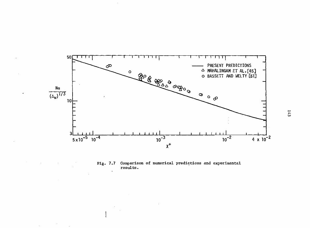
bO 1 1 1 1 1 1 1 1 1 1 1 1 1 1 1 1 1 1 1 1 1 1 1 1 1
Nu
10
PRESENT PREDICTIONS O ^ MAHALINGAM ET AL.[45]
^ o BASSETT AND WELTY [61]
—
3 1 i 1 1 1 1 1 1 1 1 1 1 1 1 1 1 1 1 1 1 1 1 1 1 1
-
5x10"^ 10"^ 10"^ 10"^ 4 X 10
Fig. 7.7 Comparison of numerical predictions and experimental results.

— NUMERICAL PREDICTIONS, n = 1
Û HAHALINGAH ET AL. [45]
o BASSETT AND HELTY [61]
— 9 0 S C O N F I D E N C E B A N D S O N D A T A
1/3
EQ. (7.6)
1 2 4 3 4 10 10 5 X 10 10
Fig, 7.8 Comparison of present experimental data and numerical predictions with available experimental data.
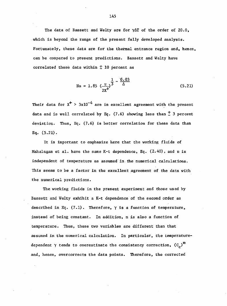
145
The data of Bassett and Welty are for of the order of 20.0,
which is beyond the range of the present fully developed analysis.
Fortunately, these data are for the thermal entrance region and, hence,
can be compared to present predictions. Bassett and Welty have
correlated these data within i 10 percent as
1 - 0.03
Nu = 1.85 (-0-) (5.21) 2X+
Their data for > 3x10" are in excellent agreement with the present
data and is well correlated by Eq. (7.6) showing less than t 3 percent
deviation. Thus, Eq. (7.6) is better correlation for these data than
Eq. (5.21).
It is important to emphasize here that the working fluids of
Mahalagam et al. have the same K-t dependence, Eq. (2.40), and n is
independent of temperature as assumed in the numerical calculations.
This seems to be a factor in the excellent agreement of the data with
the numerical predictions.
The working fluids in the present experiment and those used by
Bassett and Welty exhibit a K-t dependence of the second order as
described in Eq. (7.1). Therefore, y is a function of temperature,
instead of being constant. In addition, n is also a function of
temperature. Thus, these two variables are different than that
assumed in the numerical calculation. In particular, the temperature-
dependent Y tends to overestimate the consistency correction, (C )™
and, hence, overcorrects the data points. Therefore, the corrected

146
non-Newtonian data points lie below the constant property Newtonian
predictions. The effect of temperature-dependent Y is particularly
significant in the early part of the entrance region. In spite of
these discrepancies in the numerical assumptions and experimental
characteristics, the data are in excellent agreement for X" > 10" ,
while for X"*" < 10" the deviation is not very large. Therefore, over
the entire thermal length, the results of the numerical predictions
give sufficient accuracy for design purposes. Therefore, constant
property Newtonian predictions* with non-Newtonian correction and
consistency correction are recommended for design purposes.
Conclusions
Heat transfer in laminar in-tube flow of non-Newtonian pseudo-
plastic fluid was studied. An extensive experimental data were
obtained (144 points) for two HEMC solutions in two different tubes
for the entire thermal length. In this case, the heat transfer
coefficients are substantially higher than the constant property
Newtonian predictions. This increase above the Newtonian results is
accounted for by applying the following corrections:
1) Non-Newtonian correction, This correction is generally
small.
2) Variable consistency index correction (C )™. This correction
is quite significant.
With these two corrections, non-Newtonian experimental data are in
excellent agreement with the constant property Newtonian predictions

147
for > 10 For the data lie below the numerical predictions.
At = 10" , the discrepancy is of the order of 15.0 percent. A
Statistical analysis at 90 percent confidence was done to demonstrate the
goodness of the data and the data were correlated by Eq. (7.6).
The data of Mahalingam et al. [45] are in excellent agreement with
the numerical predictions, while data of Bassett and Welty [61] in
excellent agreement with the present data. This is because the analytical
assumption and working fluid characteristics for K-t and n-t dependence
are precisely the same for the data of Mahalingam et al. There is
some discrepancy in these characteristics of working fluids for the data
of Bassett and Welty. In spite of this, their data are in fairly good
agreement with the predictions. Thus, for the entire thermal length,
the present experimental data and other data [45,61] are in sufficiently
good agreement with the numerical predictions and, hence, constant
property Newtonian predictions with non-Newtonian and consistency
corrections are recommended for design purposes.

148
CHAPTER VIII. CONCLUSIONS AND RECOMMENDATIONS
This study deals with the heat transfer in laminar in-tube flow of
non-Newtonian (pseudoplastic) fluids. The tube wall was subjected to
the uniform wall heat flux boundary condition. This is a numerical
and experimental study; the theoretical and experimental results are com
pared. Previous analyses and test results are also compared with the re
sults of this study. The following conclusions can be drawn:
1) A stable, explicit, numerical scheme was developed, using the
Dufort-Frankel finite-difference technique to solve this problem. The
usual boundary layer assumptions were made. A constant property analysis
was done for n = 1.0, 0.75, 0.5, and 0.25. This analysis indicated that
there is an increase in the heat transfer coefficient due to pseudo-
plasticity, which can be accounted for by employing a non-Newtonian
1/3 correction, A . It is important to point out that this correction is
valid up to n = 0.1, but most engineering fluids have n > 0.25, thus,
this correction can be used for most engineering calculations.
2) For the variable property analysis, it was assumed that
K = a exp (-bt) (2.40)
and a dimensionless parameter yAT, Eq. (4.9), was defined for a UHF
condition. The predictions were obtained for various values of y T
and for n = 1.0, 0.75, and 0.5. It was demonstrated that
= f(n,X+, K, /K , yAT) (4.11) Nu D w cp
A two-step method was employed to correlate these predictions:

149
For the entrance region
m = 0.58 - 0.44n (4.12)
and for the fully developed region
'k (4.20)
A generalized consistency correction, (C )™, was developed, Eq. (4.22), to
account for the increment in the Nusselt number due to consistency index
to account for the increase in the non-Newtonian Nusselt number above
the constant property Newtonian prediction.
3) For the Newtonian case alone, with variable u, an additional
analysis was made for the fully developed region. The predictions of
this analysis are in excellent agreement with other predictions obtained
using the Dufort-Frankel marching scheme.
4) For the fully developed case, predictions for various n values
and for various yAT values are correlated to obtain z non-iterative
explicit solution as given in Eq. (4.20). This solution has significant
advantages over previous iterative solution (Eq. (4.10)), and is highly
useful for design purposes.
5) The heat transfer experiments were conducted for 0.9 percent
and 1.0 percent HEMC solutions. Nusselt numbers for these solutions, for
the entire thermal length, are substantially higher than those for the
constant property Newtonian Nusselt numbers. To these non-Newtonian
Nusselt numbers, the non-Newtonian correction, (A )and the temperature'
variation. Thus, two corrections, namely, and (C )™, were employed

150
dependent consistency index correction, (C )®, was applied and plottedi
in Fig. 7.6. It is seen that these corrected Nusselt numbers are in
excellent agreement with constant property Newtonian predictions for
X"*" > 10" , while for X" < 10 the experimental data lie somewhat lower
than the numerical predictions. In general, the experimental data are in
sufficiently good agreement with numerical predictions. Therefore,
constant property Newtonian predictions with non-Newtonian and
consistency index corrections are recommended for design purposes.
6) The data of Mahalingam et al. [45] are in excellent agreement
with the numerical predictions. The assumptions of the numerical analysis
correspond to the characteristics of the methocel solution used by •
Mahalingam et al., namely the K-t relation as given in Eq. (2.40) and n
independent of temperature. The present consistency index correction
alone corrects the numerical predictions quite well, strongly suggesting
the absence of free convection effects.
7) The data of Bassett and Welty [61] are in excelleng agreement
with the present data. Most of their data are for X"*" < 10" . The
maximum discrepancy between their data and the present numerical solution
seems to occur at X" = 10" and it is of the order of 15 percent.
8) The present data and data of Bassett and Welty lie below
numerical predictions for X+ < 10" . The present working fluids and the
5. 4 percent methocel solution used by Bassett and Welty exhibit a weak
temperature dependence of n and K-t relation as given in Eq. (7.1). This
proposed correction factors thus tend to overcorrect data in the early
part of the entrance region. However, this deviation is not
151
substantial and, therefore, numerical predictions are sufficiently
accurate for the design purposes.
9) Finally, it can be concluded that there is good agreement
between numerical predictions and various experimental data. A
generalized correlation method is developed from the numerical
predictions to correlate Nusselt numbers for various n values and a
wider range of heat fluxes.
Although this study has shown a good agreement between the experi
mental data and numerical solution which can be used for design
purposes, further work can be pursued in the following areas
1) A similar explicit numerical analysis is required for a UWT
boundary condition and needs to be compared with available predictions
and experimental data.
2) In this study, results are obtained for the in-tube heating
of pseudoplastic fluids. Many industrial applications involve the
cooling of pseudoplastic fluids. These heating results are also probably
applicable to the case of cooling. However, experimental data need
to be obtained for this cooling case and compared with the numerical
predictions.
3) A second-order K-t relation needs to be incorporated in the
numerical scheme such as
K = a exp (-bt - ct^) (7.1)
4) Bingham plastic represents a major class of non-Newtonian fluids.
A similar analytical and experimental study is required for these fluids.
152
5) Laminar flow is inherently associated with low magnitudes of
heat transfer coefficients. Recently, there have been many studies
dealing with augmentation of heat transfer in Newtonian in-tube flow
[102,103]. A substantial improvement in the heat transfer performance is
demonstrated by employing various static mixers. A similar augmentation
study for non-Newtonian fluids is required.

153
BIBLIOGRAPHY
1. Skelland, A. H. P. Non-Newtonian Flow and Heat Transfer. New York; John Wiley and Sons, Inc., 1967.
2. Kays, W. M. Convectlve Heat and Mass Transfer. New York: McGraw-Hill Book Company, 1966.
3. McAdams, W. H. Heat Transmission. 3rd edition. New York; McGraw-Hill Book Company, 1954.
4. Graetz, L. "Uber die Warmeleitungsfahigkeit Von Flussigkiten." Annalen der Physik 23 (1883); 79-94.
5. Graetz, L. "Uber die Warmeleitungsfahigkeit Von Flussigkiten." Annalen der Physik 25 (1885); 337-357.
6. Nusselt, W. "Die Abhangigkeit der Warmeiibergangszahl von der Rohrlange." Zietschrift des Vereines Deutscher Ingenieure 54 (1910): 1154..
7. Leveque, A. "Les Lois de la Transmission de Chaleur par Convection." Annales des Mines Paris-Mem. Ser. 12, 13 (1928); 283-290.
8. Kays, W. M. "Numerical Solutions for Laminar Flow Heat Transfer in Circular Tubes." Transactions of ASME 77 (1955); 1254-1274.
9. Wors^e-Schmidt, P. M. "Heat Transfer in the Thermal Entrance Region of Circular Tubes and Annular Passage with Fully Developed Laminar Flow." International Journal of Heat and Mass Transfer 1(1967): 541-551.
10. Sellars, J. R.; Tribus, M. and Kline, J. S. "Heat Transfer to Laminar Flow in Round Tube Flat Conduit - the Graetz Problem Extended." Transactions of ASME 78 (1956): 441-448.
11. Siegel, R., Sparrow, E. M. and Hallman, T. M. "Steady Laminar Heat Transfer in a Circular Tube with Prescribed Wall Heat Flux." Applied Scientific Research A7 (1958); 385-392.
12. Ulrichson, D. L. and Schmitz, R. A. "Laminar-Flow Heat Transfer in the Entrance Region of a Circular Tube." International Journal of Heat and Mass Transfer 8 (1968): 253-258.
13. Hombeck, R. W. "An All-Numerical Method for Heat Transfer in the Inlet of a Tube." ASME Paper No. 65-WA/HT-36 (1965).
14. Roy, D. N. "Development of Laminar Flow in Circular and Coaxial Tubes with and without Heat Transfer." Ph.D. Thesis, University of Calcutta, Bengal Engineering College, Weat Bengal, India, 1966.

154
15. Manohar, R. "Analysis of Laminar-Flow Heat Transfer in Entrance Region of Circular Tubes." International Journal of Heat and Mass Transfer 12 (1969): 15-22.
16. Butterworth, D. and Hazel, T. D. "Forced Convective Laminar Flow Heat Transfer in the Entrance Region of a Tube." AERE-R6057 Harwell 1969.
17. McMordie, R. K. and Emery, A. F. "A Numerical Solution for Laminar Flow Heat Transfer in Circular Tubes with Axial Conduction and Developing Thermal and Velocity Fields." Journal of Heat Transfer 89 (1967): 11-16.
18. Tien, C. and Pawelek, R. A. "Laminar Flow Heat Transfer in the Entrance Region of Circular Tubes." Applied Scientific Research A13 (1964); 317-331.
19. Singh, R. N. "Heat Transfer by Laminar Flow in a Cylindrical Tube." Applied Scientific Research A7 (1958): 325-340.
20. Munakata, T. "The Calculation of Laminar Heat Transfer in a Tube." International Chemical Engineering 15, No. 1 (1975): 193-196.
21. Hsu, C. J. "An Exact Analysis of Low Peclet Number Thermal Entry Region Heat Transfer in Transversely Non-Uniform Velocity Fields." AIChE Journal 17, No. 3 (1971): 732-740.
22. Beek, W. J. and Eggink, R. "Warmteoverdracht Naar een Laminaire Stroming Van een Neit-Newtonse Vloeistof in enn Ronde Buise." De Ingenuir, Chemische Techniek 7 (1962): 81-89.
23. Grigull, U. V. "Warmeiibergang an Nicht-Newtonsche Flusslgkeiten bei Laminar Rohrstromung." Chemie-Ingenieur-Technik 8/9 (1956)): 553-556.
24. Kutateladze, S. S.; Khabakhpasheva, Ye. M.; Popov, V. I.; Gruzdeva, I. M. and Perepelitsa, B. V. "Hydraulic Resistance and Heat Transfer in Stabilized Flow of Non-Newtonian Fluids." Heat Transfer, Soviet Research 2, No. 6 (1970): 114-123
25. Pigford, R. L. "Nonisothermal Flow and Heat Transfer Inside Vertical Tubes." Chemical Engineering Progress Symposium 51, No. 17 (1955): 79-92.
26. Lyche, B. C. and Bird, R. B. "The Graetz-Nusselt Problem for a Power Law Non-Newtonian Fluid." Chemical Engineering Science 6, (1956): 35-41.

155
27. Whiteman, I. R. and Drake, W. G. "Heat Transfer to Flow in a Round Tube with Arbitrary Velocity Distribution." Transactions of ASME 80. (1958); 728-732.
28. McKillop, A. A. "Heat Transfer Laminar Flow of Non-Newtonian Fluids in Entrance Region of a Tube." International Journal of Heat and Mass Transfer 7 (1964): 853-862.
29. Korayem, A. Y. "Non-Isothermal Laminar Flow of Non-Newtonian Fluids in the Entrance Region of Pipe." Ph.D. Thesis, University of California, Davis, 1965.
30. Cochrane, G. F. "A Numerical Solution for Heat Transfer to Non-Newtonian Fluids with Temperature Dependent Viscosity for Arbitrary Conditions of Heat Flux and Surface Temperature." Ph.D. Thesis, Oregon State University, 1969.
31. Mizushina, T.; Ito, R.; Kuriwake, Y. and Yahikazawa, K. "Boundary Layer Heat Transfer in a Circular Tube to Newtonian and Non-Newtonian Fluids." Kagaku Kogaku 31 (1967): 250-255.
32. Yang, K. T. "Laminar Forced Convection of Liquids in Tubes with Variable Viscosity." Journal of Heat Transfer 84 (1962): 353-362.
33. Deissler, R. G. "Analytical Investigation of Fully Developed Laminar Flow in Tubes with Heat Transfer with Fluid Properties Variable along the Radius." NACA TN 2410. 1951.
34. Shannon, R. L. and Depew, C. A. "Forced Laminar Flow Convection in a Horizontal Tube with Variable Viscosity and Free Convection Effects." Journal of Heat Transfer 91 (1969): 251-258.
35. Test, F. L. "Laminar Flow Heat Transfer and Fluid Flow for Liquids with Temperature Dependent Viscosity." Journal of Heat Transfer 90 (1968); 385-392.
36. Rosenberg, D. E. and Heliums, J. D. "Flow Development and Heat Transfer in Variable Viscosity Fluids." Industrial and Engineering Chemistry Fundamentals 4 (1965): 417-422.
37. Martin, B. W. and Fargie, D. "Effect of Temperature-Dependent Viscosity on Laminar Forced Convection in the Entrance Region of a Circular Pipe." The Proceedings of the Institution of Mechanical Engineers 186. No. 24 (1972): 307-316.
38. Sieder, E. N. and Tate, G. E. "Heat Transfer and Pressure Drops of Liquid in Tubes." Industrial and Engineering Chemistry 28 (1936): 1429-1435.

156
39. Christiansen, E. B. and Craig, S. E., Jr. "Heat Transfer to Pseudoplastic Fluids in Laminar Flow." AIChE Journal 8, 1402 (1962): 154-160.
40. Christiansen, E. B.; Jensen, G. E. and Tao, F. S. "Laminar Flow Heat Transfer." AIChE Journal 12, No. 6 (1966): 1196-1202.
41. Forrest, G. and Wilkinson, W. L. "Laminar Heat Transfer to Power Law Fluids in Tubes with Constant Wall Temperature." Transactions of the Institution of Chemical Engineers 51 (1973): 331-338.
42. Kwant, P. B.; Zwaneveld, A. and Dijkstra, F. C. "Non-Isothermal Laminar Pipe Flow-I Theoretical." Chemical Engineering Science 28 (1973): 1303-1316.
43. Popovska, F. and Wilkinson, W. L. "Laminar Heat Transfer to Newtonian and Non-Newtonian Fluids in Tubes." Chemical Engineering Science 32 (1977): 1155-1164.
44. Forrest, G. and Wilkinson, W. L. "Laminar Heat Transfer to Power Law Fluids in Tubes with Constant Wall Heat Flux." Transactions of the Institution of Chemical Engineers 52 (1974): 10-16.
45. Mahalingam, R.; Tilton, L. 0. and Coulson, J. M. "Heat Transfer in Laminar Flow of Non-Newtonian Fluids." Chemical Engineering Science 30 (1975): 921-929.
46. Bader, H. J. "Heat Transfer in Non-Newtonian Fluids with Temperature Dependent Viscosity." M.S. Thesis, University of California, Davis, 1965.
47. McKillop, A. A.; Harper, J. C.; Bader, H. J. and Korayem, A. Y. "Variable Viscosity Entrance-Region Flow of Non-Newtonian Liquids." International Journal of Heat and Mass Transfer 13 (1970): 901-909.
48. Bader, H. J.; McKillop, A. A. and Harper, J. C. "An Experimental and Analytical Study of Entrance Flow of Non-Newtonian Fluids." Heat Transfer Conference, Vol. IV, Paper No. Rh 1, Paris-Versailles, 19 70.
49. Fletcher, R. H. "On Finite-Difference Solution for the Constant-Property Turbulent Boundary Layer." AIAA Journal 7, No. 2 (1969): 305-311.
50. Dufort, E. C. and Frarikel, S. P. "Stability Conditions in the Numerical Treatment of Parabolic Differential Equations." Mathematical Tables Aids Computation 7 (1953): 135-153.

157
51. Nelson, R. M. "An Explicit Finite Difference Analysis for Developing Turbulent Internal Flows with Heat Transfer and Property Variation." M.S. Thesis, Iowa State University, Ames, May, 1972.
52. Fletcher, R. H. and Nelson, R. M. "Heat Transfer to Laminar and Turbulent Flow in Tubes with Variable Fluid Properties." Proceedings of the Fifth International Heat Transfer Conference, Tokyo, Japan II, Paper No. FC 4.5 (1974): 146-150.
53. Hong, S. W. "Laminar Flow Heat Transfer in Ordinary and Augmented Tubes." Ph.D. Thesis, Iowa State University, Ames, Iowa, 1974.
54. Hong, S. W. and Bergles, A. E. "Analysis of Combined Forced and Free Laminar Convection in Horizontal Tubes." Heat Transfer Laboratory Report, HTL-4, ISU-ERI-Ames-741555, Iowa State University, 1974.
55. Hong, S. W. and Bergles, A. E. "Analysis of Combined Forced and Free Convection in the Entrance Region of Horizontal Tubes," Recent Advances in Engineering Science. Proc. Annual Meeting of the Society of Engineering Science, Inc., Bethlehem, Pa. 14 (Nov. 1977): 453-469.
56. Richtmyer, R. D. and Morton, K. W. Difference Methods for Initial-Value Problems, 2nd edition. New York: Wiley, 1967.
57. O'Brien, G. G.; Hyman, M. A. and Kaplan, S. "A Study of the Numerical Solution of Partial Differential Equations." Journal of Mathematics and Physics 29 (1951): 223-241.
58. Madni, I. K. "A Finite-Difference Analysis of Turbulent, Axisym-metric. Buoyant Jets and Plumes." Ph.D. Thesis, Iowa State University, Ames, 1975.
59. Metzner, A. B. and Reed, J. C. "Flow of Non-Newtonian Fluids -Correlation of the Laminar, Transition, and Turbulent-Flow Regions." AIChE Journal 4 (1955): 434.
60. Metzner, A. B. "Heat Transfer in Non-Newtonian Fluids." Advances in Heat Transfer, pp. 357-397. Vol. 2. Edited by J. P. Hartnett and T. F. Irvine, Jr. New York': Academic Press, 1965.
61. Bassett, C. E. and Welty, J. R. "Non-Newtonian Heat Transfer in che Thermal Entrance Region of Uniformly Heated Horizontal Pipes." AIChE Journal 21, No. 4 (1975): 699-706.

158
62. Keevll, C. S. and McAdams, W. H. "How Heat Transmission Affects Fluid Friction in Pipes." Chemical and Metallurgical Engineering 36 (1929): 464.
63. Kirkbride, C. G. and McCabe, W. L. "Heat Transfer to Liquids in Viscous Flow." Industrial and Engineering Chemistry 23 (1931); 625-631.
64. Drew, T. B. "Heat Transfer in Stream Line Flow - II - Experiments with Glycerol." Industrial and Engineering Chemistry 24 (1932): 152-157.
65. Colbum, A. P. "Forced Convection Heat Transfer Data." Transactions of AIChE 29 (1933): 174-210.
66. Kern, D. Q. and Othmer, D. F. "Effect of Free Convection on Viscous Heat Transfer in Horizontal Tubes." Transactions of AIChE 39 (1943): 517-555.
67. Eubank, 0. C. and Proctor, W. S. "Effect of Natural Convection on Heat Transfer with Laminar Flows in Tubes." S. M. Thesis in Chemical Engineering, M.I.T., 1951.
68. Oliver, D. R. "The Effect of Natural Convection on Viscous Flow Heat Transfer in Horizontal Tubes." Chemical Engineering Science 17 (1962): 335-350.
69. Brown, A. R. and Thomas, M. A. "Combined Free and Forced Convection Heat Transfer for Laminar Flow in Horizontal Tubes." Journal of Mechanical Engineering Science 7, No. 4 (1965): 440-448.
70. Depew, C. A. and August, S. E. "Heat Transfer Due to Combined Free and Forced Convection in a Horizontal and Isothermal Tube." Journal of Heat Transfer 97 (1971): 380-384.
71. Jackson, T. W.; Spurlock, J. M. and Purdy, K. R. "Combined Free and Forced Convection in a Constant Temperature Horizontal Tube." Journal of the American Institute of Chemical Engineers 7 (1961): 38-45.
72. McComas, S. T. and Eckert, E. R. G. "Combined Free and Forced Convection in a Horizontal Circular Tube." Journal of Heat Transfer 88 (1966): 147-153.
73. Mori, Y.; Futagami, K.; Tokuda, S. and Nakamura, M. "Forced Convective Heat Transfer in Uniformly Heated Horizontal Tubes, 1st Report-Experimental Study on the Effect of Buoyancy." International Journal of Heat and Mass Transfer 12 (1969): 1535-1552.
158
62. Keevil, C. S. and McAdams, W. H. "How Heat Transmission Affects Fluid Friction in Pipes." Chemical and Metallurgical Engineering 36 (1929): 464.
63. Kirkbride, C. G. and McCabe, W. L. "Heat Transfer to Liquids in Viscous Flow." Industrial and Engineering Chemistry 23 (1931); 625-631.
64. Drew, T. B. "Heat Transfer in Stream Line Flow - II - Experiments with Glycerol." Industrial and Engineering Chemistry 24 (1932): 152-157.
65. Colburn, A. P. "Forced Convection Heat Transfer Data." Transactions of AIChE 29 (1933): 174-210.
66. Kern, D. Q. and Othmer, D. F. "Effect of Free Convection on Viscous Heat Transfer in Horizontal Tubes." Transactions of AIChE 39 (1943): 517-555.
67. Eubank, 0. C. and Proctor, W. S. "Effect of Natural Convection on Heat Transfer with Laminar Flows in Tubes." S. M. Thesis in Chemical Engineering, M.I.T., 1951.
68. Oliver, D. R. "The Effect of Natural Convection on Viscous Flow Heat Transfer in Horizontal Tubes." Chemical Engineering Science 17 (1962): 335-350.
69. Brown, A. R. and Thomas, M. A. "Combined Free and Forced Convection Heat Transfer for Laminar Flow in Horizontal Tubes." Journal of Mechanical Engineering Science 7, No. 4 (1965): 440-448.
70. Depew, C. A. and August, S. E. "Heat Transfer Due to Combined Free and Forced Convection in a Horizontal and Isothermal Tube." Journal of Heat Transfer 97 (1971): 380-384.
71. Jackson, T. W.; Spurlock, J. M. and Purdy, K. R. "Combined Free and Forced Convection in a Constant Temperature Horizontal Tube." Journal of the American Institute of Chemical Engineers 7 (1961): 38-45.
72. McComas, S. T. and Eckert, E. R. G. "Combined Free and Forced Convection in a Horizontal Circular Tube." Journal of Heat Transfer 88 (1966): 147-153.
73. Mori, Y.; Futagami, K.; Tokuda, S. and Nakamura, M. "Forced Convective Heat Transfer in Uniformly Heated Horizontal Tubes, 1st Report-Experimental Study on the Effect of Buoyancy." International Journal of Heat and Mass Transfer 12 (1969): 1535-1552.
159
74. Hussain, N. A. and McComas, S. T. "Experimental Investigation of Combined Convection in a Horizontal Circular Tube with Uniform Heat Flux." Heat Transfer Conference, Vol. IV, Paper No. NC 3.4, Paris-Versailles, 1970.
75. Lichtarowicz, A. "Combined Free and Forced Convection Effects in Fully Developed Laminar Flow in Horizontal Tubes." Heat and Mass Transfer by Combined Forced and Free Convection, Paper No. C114/71. London, Institution of Mechanical Engineers, 1972.
76. Ede, A. J. "The Heat Transfer Coefficient for Flow in a Pipe." International Journal of Heat and Mass Transfer 4 (1961); 105-110.
77. Petukhov, B. S. and Polyakov, A. F. "Experimental Investigation of Viscogravitational Fluid Flow in a Horizontal Tube." High Temperature 5 (1967); 75-81.
78. Petukhov, B.S. and Polyakov, A. F. "Effect of Free Convection on Heat Transfer during Forced Flow in Horizontal Pipe. " High Temperature 5 (1967): 348-351.
79. Petukhov, B. S.; Polyakov, A. F. and Strigin, B. K. "Heat Transfer in Tubes with Viscous-Gravity Flow." Heat Transfer-Soviet Res earch 1 (1969): 24-31.
80. Shannon, R. L. and Depew, C. A. "Combined Free and Forced Laminar Convection in a Horizontal Tube with Uniform Heat Flux." Journal of Heat Transfer 90 (1968); 353-357.
81. Bergles, A. E. and Simonds, R. R. "Combined Forced and Free Convection for Laminar Flow in Horizontal Tubes with Uniform Heat Flux." International Journal of Heat and Mass Transfer 14 (1971): 1989-2000.
82. Siegwarth, D. P.; Miskell, R. D.; Redal, T. C. and Hanratty, T. J. "Effect of Secondary Flow on the Temperature Field and Primary Flow in a Heated Horizontal Tube." International Journal of Heat and Mass Transfer 12 (1969): 1535-1552.
83. Morcos, S. M. and Bergles, A. E. "Combined Forced and Free Laminar Convection in Horizontal Tubes." Heat Transfer Laboratory Report, HTL-1, ISU-ERI-Ames-74008, Iowa State University, 1974.
84. Morcos, S. M. and Bergles, A. E. "Experimental Investigation of Combined Forced and Free Laminar Convection in Horizontal Tubes." Journal of Heat Transfer 97 (1975): 212-219.
85. Porter, J. E. "Heat Transfer at Low Reynolds Number (Highly Viscous Liquids in Laminar Flow) Industrial Research Fellow Report." Transactions of the Institution of Chemical Engineers 49 (1971): 1-29.

160
86. Froishteter, G. B. and Smorodlnskii, E. L. "Laminar Heat Transfer of Non-Newtonian Liquids in Tubes with Variable Physical Properties." Translated from Teoretlcheskir Osnovy Khimicheskoi Tekhnologii 9. No. 3 (1975): 392-405.
87. Metzner, A. B.; Vaughn, R. D. and Houghton, G. L. "Heat Transfer to Non-Newtonian Fluids." AIChE Journal 3, No. 1 (1957): 92-100.
88. Charm, S. E. "Calculation of Centre-Line Temperatures in Tubular Heat Exchangers for Pseudoplastic Fluids in Streamline Flow." Industrial and Engineering Chemistry Fundamentals 1, No. 2 (1962); 79-82.
89. Charm, S. E. and Merrill, E. W. "Heat Transfer Coefficients in Straight Tubes for Pseudoplastic Food Materials in Streamline Flow." Food Research 24 (1959): 319-331.
90. Gluck, D. F. "The Effect of Turbulence Promotion on Newtonian and Non-Newtonian Heat Transfer Rates." M. Ch. E. Thesis, University of Delaware, 1959.
91. Metzner, A. B. and Gluck, D. F. "Heat Transfer to Non-Newtonian Fluids under Laminar Flow Conditions." Chemical Engineering Science 2 (1960): 185-190.
92. Oliver, D. R. and Jens on, V. G. "Heat Transfer to Pseudoplastic Fluids in Laminar Flow in Horizontal Tubes." Chemical Engineering Science 9 (1964): 115-129.
93. Junkhan, G= H. and Bergles, A. E. "Heat Transfer Laboratory Data Acquisition System." Heat Transfer Laboratory Report, HTL-12, ISU-ERI-77178, Iowa State University, December, 1976.
94. Uhl, V. W. and Root, W. L. "Heat Transfer in Hollow Cut-Flight Jacketed Units to Viscous Fluids." Chemical Engineering Progress Symposium Series 102, vol. 66 (1970): 199-206.
95. Amato, W. S. and Tien, C. "Free Convection Heat Transfer from Isothermal Spheres in Polymer Solutions." International Journal of Heat and Mass Transfer 19 (1976): 1257-1266.
96. Oliver, D. R. and Asghar, S. M. "The Laminar Flow of Newtonian and Viscoelastic Liquids in Helical Coils." Transactions of the Institution of Chemical Engineers 53 (1975): 181-186.
97. Lipson, C. and Seth, N. J. Statistical Design and Analysis of Engineering Experiements. First edition. New York: McGraw-Hill Book Company, 1973.

161
98. Cook, N. H. and Rabinowicz, e. Physical Measurement and Analysis. London: Addison Wesley Publishing Company, Inc., 1963.
99. Churchill, S. W. and Usagi, R. "A General Expression for the Correlation of Rates of Transfer and Other Phenomena." AIChE Journal 18, No. 6 (1972); 1121-1128.
100. Mischke, C. and Hall, J. L. ISU Cadet Program ME 0226. Department of Mechanical Engineering, Iowa State University, Ames, Iowa, 1975.
101. Churchill, S. W. and Ozoe, H. "Correlations for Laminar Forced Convection in Flows over a Uniformly Heated Plate and in Developing and Fully Developed Flow in a Tube." ASME Paper No. 72-WA/HT-14, 1973.
102. Bergles, A. E. "Laminar Flow Heat Transfer in Horizontal Tubes under Normal and Augmented Conditions." Heat Transfer Laboratory Report, HTL-11, ISU—ERI-Ames—77179, Iowa State University, 1975.
103. Hong, S. W. and Bergles, A. E. "Augmentation of Laminar Flow Heat Transfer in Tubes by Means of Twisted-Tape Inserts." Journal of Heat Transfer 98 (1976): 251-256.
104. Handbook on Methocel. Midland, Mich.: Dow Chemicals, 1975.
105. Scheve, J. L. "A Simplified Process Viscometer for Non-Newtonian Fluids." M.S. Thesis, Iowa State University, 1971.
106. A.S.M.E. Steam Tables. New York: A.S.M.E., 1967.

162
ACKNOWLEDGMENTS
I take this opportunity to express my gratitude to Dr. A. E. Bergles,
Chairman of the Mechanical Engineering Department, for his invaluable
guidance and supervision at all stages of this work.
I am thankful to Dr. R. H. Fletcher and Dr. J. L. Hall with whom I
had many useful sessions of discussion. I am also thankful to Dr. G. H.
Junkham and Dr. D. F. Young for their help during the course of this
work.
I am also thankful to Mr. Hap Steed of the Mechanical Engineering
Department and Mr. Leon Girard and associates from the Engineering Research
Institute workshop for their earnest co-operation and pains they have
taken to rectify the troubles encountered during the fabrication of the
experimental setup. Thanks are also due to Miss Mary Smith for her neat
typing of this thesis.
The financial support given by the Engineering Research Institute,
the Power Affiliate Program, and the Department of Mechanical Engineering
during the course of this study is greatly appreciated.
Last, but not the least, I am greatly indebted to my parents,
brothers, and sisters, for their constant encouragement and affection.
I am especially grateful to my parents, Mr. and Mrs. D. M. Joshi, for
the inspiration, love, and motivation they provided for my higher
education, since the early days of my life.
This thesis is humbly dedicated to my parents, to whom I owe all
that I know.

163
APPENDIX A: FINITE-DIFFERENCE EQUATIONS
Dufort-Frankel Formulation
A Dufort-Frankel finite-difference formulation of the non-
dimensional momentum, energy, and continuity equations, Eqs. (3.8a) to
(3.10) is given here.
Momentum
2. .u , ,, . i.j i,j + Ax_) (AY+ + AY_)
(^i+1 - Pi-l)
(AX+ + AX_) (AY+ + AY_) (A.l)
^^j+1 (^a,i,j+l •*" Ua,i,j)(Oi^j+i - 0.5 + "i-l,j^^
AYj
. (*j + *j_l)(Va,i,j+Wa,i.j-l) (0.5 - Ujj.i)
4 AY

164
Energy
3. . u; . c, 1. V, .8 . i,J i,J P i »J (AX+ + AX_) P ' J (Ay++ AY_)
1 2 Rj (AY^ + AY_)
(A. 2)
Oy+1 + Rj)(Sl, j+l + ki, j)(Ti, j+l - 0-5 (Ti+l, j + Ti_l. j))
AY,
(R. + Rj_i)(k.,. + ki,j_l)(0.5 (T.+i,j + Vl,j> -
AY_
+ U a , i , ]
AY+ + AY_
Continuity
(Rj+1 + Rj)
4(AX+ + Ax_)
AY^ (A. 3)

165
Comments on Dufort-Frankel Momentum' Equation
In all of the above equations, non-dimensional apparent viscosity is
^"i,j+l ~ i,j-l)
''a.io" — (AY+ + .AY_)
n-1
(3.8b)
where (y^ is the apparent viscosity at the wall at the tube inlet.
The scheme given by Eq. (A.l) does not adhere to the Dufort-Frankel
differencing in the strict sense. Equation (3.8b) shows that while
evaluating y j and y . . a term U. • will be in a derivative '^a,i,j+l a,i,]-i i»J
form and it would appear that this U. . should be averaged as
((Ui^l j + j) /2) to be consistent with the Dufort-Frankel
differencing. This would require a much more complex solution for
^i+1 j Eq. (A.l) due to the non-linearity of the algebraic system.
Nelson [51] has shown for the turbulent flow that Eq. (A.l) may be used
and this equation will remain stable if the y . .'s used are the a,x,j
average of P^.i^-l' a.i.j ya,i,j+l-
In Eq. (3.8b), for n = 1, the exponent of 9u/9y term vanishes and,
hence, 9u/9y has no influence on the local viscosity. For n = 0.5, the
exponent of 9u/9y is -0.5, and, therefore, it will influence the local
viscosity to some extent; however, without using averages as suggested
by Nelson, Eq. (A.l) was found to be stable.
For n = 0.25, the exponent of 9u/9y is -0.75 and, therefore, the
term 9u/3y plays a dominant role in determining the value of local
viscosity. This y^ dependence on 3u/3y is analogous to one observed in
turbulent flows. At lower values of n (n < 0.5), Eq. (A.l) was used

16 Ô
without averaging for and a substantial instability was noticed.
This instability was eliminated by taking averages of viscosities, as
suggested by Nelson.
Standard Explicit Finite-Difference Equations
The standard explicit form of the momentum equation used in the
starting procedure (normally the first ten steps) is
'J Air 1 ) j AX+ AY_
R. (AY+ + AYJ (A. 4)
(Rj + Rj+i)(Wa,i,j+Ua,i,j+l)(Hi,j+i - Ui,j)
4 AY^
(R. +Rj_i)(Wa,i,j+1^a,i,j_l)(Ui,j - Ui,j_l)
ay_
The starred term is used when V- • is positive; otherwise, to maintain
stability it is replaced by

167
The standard explicit form of the energy equation is
R. (AY. + AY ) J + -
(A.5)
4 AY,
(Rj H- Rj-j) (k,_ . + - Tj.j-l)
4 /a_
Ay
y . . is calculated the same way as in the Dufort-Frankel J
formulation, although the averaging is not really necessary.
The continuity equation for the ordinary explicit method is
(Rj+1
Ax. <«>1+1,3+1 - 1.3+1 + ("«1+1.3 - ("">1.3
(A. 6)

168
APPENDIX B; TRUNCATION ERROR IN THE DUFORT-FRANKEL DIFFERENCE EQUATIONS
Consistency is studied by expanding the dependent variables in
Taylor series and estimating the truncation error. A finite-difference
scheme is said to be consistent if the truncation error vanishes as
the mesh size approaches zero. In the following analysis a uniform grid
spacing in the radial direction is assumed. The variable U at various
grid points is expanded in Taylor series about the point (i,j) to give
the following expressions;
(B.l)
AX_ + ( ) d Uv ^
9x2
a^ut ax!
(B.2)
o 2
(B.3)

169
2 2
"i. j- i • "i . j - ^
( A ) . , M +
(B.4)
ay 3 i,j 6
To simplify, two assumptions are made:
1) AY^ = AY_
(Rj + Rj+i)(Wa_i_j + 'a,i,j+l> _ , ;
' z ra.l.j
4
The second assumption is justified since by expanding (Rj + Rj+i)
(Ûa.i.j + ïia.l.j+l) ®J + Kj-l' ®
series around the grid point (i,j), no new term appears that will alter
the truncation error.
With these assumptions, Eqs. (B.l) to (B.4) are substituted in
Eq. (A.l) to give
Î... [ ' P , . , • é " ' ^ > ' <»..! gWr: ]
• "1.1 •..! ' î<0' "']• - Ï - <$>U

170
(AX^ + Axf) ^
6(AX+ + AX_) 12
_ (AX+ - AX,) _ £n (a4 + Ax!) _ A
9x2 2(AY)2 3x^ 3x (AY)2
(Axj - Ax3)
6(AY)2
(B.5)
TEjjj is the truncation error of the momentum equation which is
estimated as
TE^ = Eq. (B.5) - Eq. (3.8)
2
3 I av3. 0 (<*1^^ 0(AY2) + 0
^ AXJ. + AX / \ AY2 / (B.6)
\ Ay2 / \ AY2 I
Now if AX_p = AX_, then Eq. (B.6) becomes
o o AX^ TE = O(AX^) + O(AY^) + 0 (—) (B.7)
AY 2
2 o The significance of the term 0 (AX /AY ) in the truncation error has
171
been discussed in Chapter III. Comparing Eqs. (B.6) and (B.7), the
advantage in using the central-difference Dufort-Frankel finite-
difference formulation is obvious. This smaller truncation error,
Eq. (B.7), can be achieved, at least approximately, by not allowing
two successive step sizes to differ significantly.
Hong [53] and Richtmyer and Morton [56] have suggested methods to
eliminate the first two terms in Eq. (B.7). These calculations were
found to be unimportant for the present calculations.
A similar analysis was done for the energy equation and TEg. The
truncation error in the energy equation reduces to
TE = O(AX^) + O(AY^) + 0(AX2/AY2) + O(AY^) (B.8) e
Here again, the consistency criterion requires that for the term AX^/AY^,
AX should go to zero faster than AY. Fortunately AX^/AY^ is associated
3^T AX^ with —r— —— . For the UHF condition, in the fully developed region 3X^ AY
2 2 2 is zero, and, hence, the term (^^) vanishes. In the thermal
9X^ 3Y^ AY^
entrance region, the terra —î is very small (this can be shown by 3Y'^
order of magnitude analysis) and, therefore, it can be neglected.
Thus, the energy equation will be consistent for - 1.

172
APPENDIX C: COMPUTATION OF PRESSURE P^^^^
It is seen from the momentum equation, (A. 1) and (A. 4), that in
order to calculate U . at any j location, the pressure at an axial 1 "f"! 5 J
location, i+1, P^^^, must be known. The integral equation of global
continuity is used to obtain this pressure. The equation of global
continuity is
m ypi+l,j "i+l,j (3.11)
The finite-difference approximations require a fine grid for
convergence and, therefore, the difference between P^+2 j j is
small enough to be neglected. Hius
Pi,j " Pi+l,j (C.l)
Substituting this in Eq. (3.11) yields
A
It will be seen later that excellent results were obtained using this
method, which indicates the usefulness and success of this approximation.
In Eq. (C.2), U.,. . is substituted from the finite-difference i+J-, J
Dufort-Frankel momentum equation, Eq. (A. 1), and then integrated by using
Simpson's rule over the entire tube cross-section. With the finite-
difference form of Uj^^^ j, the global continuity equation, Eq. (C.2),

173
has a pressure term which is only a function of axial location (i.e.,
at a given cross-section the pressure is constant), and, hence, it can be
factored out of the integration, and the following result is obtained:
" = A,3 "1+1,3 = /i ^ <Vi - /fx /N /\ ^ A A A
(C.3)
where
PA = 4 . U R. . (AY. + AY_) AY. AY_ + (AX + AX_) AY_ 1>J ' ' "T » ""
«3+1 + ^3) <®a,l,3+l + Oa.1.3) + <"+ + («3 + *j_l)
(^a,i,3 *^3,1,3-1'
PB - 4 j Rj AY+ âï. (M+ + MJ V._j
+ 2 . (M+ + M.) iY.
("1,3+1 - "1-1.3) '"i+l + Kj) + 2 1.3 <'®+ +
^^+ *"3,1.3 * "a,l,i-l) '"1,3-1 ' "1-1,3'
(E. + E..j) + 4 gZ j D..1_ , j Ej (4T^ + AY.) AY+ AY.
PC = -4 Ô. . R. (AY, + AY ) AY. AY IjJ j + - -t- -
Equation (C.3) is solved for the pressure since all other
variables are known at the i and i-1 locations. A similar procedure was

174
followed to compute the pressure in the ordinary explicit finite-
difference scheme by using the corresponding momentum equation,
Eq. (A.4).

175
APPENDIX D: COMPUTER CODE FOR CHAPTER III
In this appendix, the computer code developed to solve the problem
of heat transfer in in-tube flow of pseudoplastic fluid is given. This
computer code has a main program and six subroutines, namely,
1) DELX 1: calculates the streamwise step for starting the
ordinary explicit scheme
2) PRES : calculates pressure
3) UVEL: calculates velocity
4) TEMP: calculates temperature
5) POLFIT: fits the curve
6) Fluid Property subroutines

1-76
c THE FLLLCWING IS TFE FCRMAT TU BE USED FOR THE INPUT CARDS. c ALL FCHMATS ARE 6G12.S EXCEPT THE TITLb CARD WHICH IS 72H AKO THE c INTEGER CARDS WHICH AfiE 8110.
< c
QUANTITIES TO HE INPUT WHEN USED
C "TITLE" ALWAYS C DENS. VI SC. (.START, PS TA FT .RAC.DELY I ALWAYS C VDK.VWtOYM .PRT.CXF,DXF|, ALWAYS C SICCA ALWAYS C RCGN.TSTAkT.rwALL.CFCC^.HTK«OW DENS.LE.O C IE NO,ICLT.NSTA.KNC.NY.LORT,NT «NS ALWAYS c INPR ALWAYS C OREX.CREI.CXCUT.CINC.CSTOP ALWAYS C CUTIK ) ,K=1 .NSTA NSTA.GT.O c UO.OD1,VV1 USTART.LE.O c XVO.XVTO.AC.SPLV VISC.LT.O c CPO.CF10,CO CPCON.LT.O c HTKO,HTK10 ,dO.SPLK HTK.LT.O c TW(J) tJ=l, |NT| TCI ALL.LT.O c 7X4J) .J=l. iNTl TWALL.LT.O c
. C THE FCLLQhJNO IS AN EXFLANATIUN OF THL INPUT C C QUANTITY EXPLANAIJCN C C DENS =OENSITY(LEM/FTJ) FOR CONSTANT PROPERTY FLOW C .LE.O INDICATES VARIAULE PRCPERTV FLCN C Vise =VISCOSIT Y(L8M/FT-SEC) FOR CONSTANT VISCOSITY C .LT.O INDICATES VARIABLE VISCOSITY (DENS MUST BE .LT.O) C LSTAHT =VELOCITY(FT/SEC) FOR UNIFORM INITIAL PROFILE C .LE.O INDICATES FULLY DEVELOPED PROFILE WILL BE USED C PSTART ^INITIAL STATIC PRESSURE (L8F/FT2I C .LT.O INDICATES THAT PRESSURE OR EDGE VELOCITY C OlSTRiacTICNS WILL Ut INPUT C KAD =RADIUS FCP PIPE (FT) C =0 INDICATES FLAT PLATE C .LT.O INDICATES CHANNEL JRAD|=HALF-WIOTH C DELYI =Y GRID SPACE NEAREST THE WALL C VUK = VAN DRIEST CONSTANT K (SUGGEST USING 0.40) C VW = NORMAL VELOCITY COMPONENT TO WALL C DYM = MINIMUM V GRID OEUMcTRIC FACTOR (USED IN TURBULENT FLOW) C A DYM CF 1.C4 (LARGER FOR FLAT PLATE) FOR INPUT IS GOOD. C THE ADJUSTED DYM (HECACSE THE SPACES MUST FILL THE WHOLE C PIPE OR CHANNEL) SHOULD NOT BE GREATER THAN 1.15 FOR MOST C CASES (l.Oe OR LESS FOR HIGH PRESSURF GRADIENT OR C HIGH HEAT TRANSFER) C DXF =OElX/(BCl,hDARY LAYER THICKNESS) kOR D-^ tUUAT lUNS C FUR LAMINA; CONSTANT PROPERTY FLCWS, C 0.0C08 TIMES THE TUBE REYNCLDS NUMBER MAY BE USED. C KAY NEED SMALLER DXF FOR HEAT TRANSFER, C .LT.O FOR CXF INCREASES SLOWLY FRCM JOXFJ C OXFM ^MAXIMUM DXF IF DXF.LT.O. OR STARTING METHOD IS USED C SAKE AS DXF C SIGMA = PARAMETER FOR CONTROLINu DELTA X IN PRESSURE GRADIENT C CASES (USUALLY = 0.003) C f-CCN =GAS CONSTANT R FOR OENSIT Y=P/RT C ,LE,0 FOR CENSXÎV--RCCN L FUR CLNSTANT DENSITY FLOW RCCN SHOULD BE NEGATIVE C TSTART =TEMPERATLFE(DEG R) FOR UNIFORM INITIAL PRCFILE

177
C TkALL =*ALL 1 EMPEfriATUkt. < Ofcti f- » HJK CCNST WALL TfcMP C =0 INDICATES CCNIjIANÎ HALL KEA1 FLUX C .LI.O FUK TEMP OH HLAT FLUX INPUT ALUNO WALL C CPCCN =SPeClFIC l-CAT (OTO/LBM-R) C .LT.O INDICATES VARIABLE. bPECIFIC HEAT C FiTK = TFERMAL CONOUCIIVITV t dT C/HH-FT-R ) C .LE.G INDICATES VARIABLE THERMAL CCNCUCTIVITV C CW =WALL HEAT FLUX (BTU /HR-FT2» FOR CONSTANT HEAT FLUX C ICND =LASI I STATION TU BE CCMPOTED C THIS IS A SAFETY FEATURE. SET lEND HIGH <1000 CR MCREI C IF A CASE MGHT NtED MORE STEPS. MOST CASES TAKE ABOUT C 400 STEPS C ICLT =NUM8ER CF I STEPS BETWEEN CUTPbT C .Lc.O NOT USED C NSTA =NUM8ER CF RFX.RET, OR X STATIONS TO BE READ IN FOR OUTPUT C .LE.O NCT USED C KKC .GT.O RE AC IN ANOTHER CASE AFTER THIS CNE C .LE.O THIS IS THE LAST CASE TO BE READ IN < NY =NUMBER (NLST BE EVEN! OF Y GRID SPACES IN PIPE CR CHANNEL C SUGGEST USING 50. MORE MAY BE NEEDED FOR SOME CASES. C NOT =NUMBER CF DATA POINTS INPUT FCR WALL TEMPERATURE C .LT.O -NCT=NUM8ER FUR HEAT FLUX C KS =1CCCNT HHEN D-F EQUATICKS START C SUGGEST CSING 20 C INPF. = 0 FOP PIPE, CHANNEL, OR FLAT PLATE CASES C = NUM3ER LF INPUT STATICNS FOR WALL RADIUS FCR BODIES C OF KEVCLLTICN C .LT.O FOR INPUT FORMULAS FOR RW AND DRW/DXA IN FUNCTION C OREX =VALUE OF BEX BETWEEN CUTPLT, OR FIRST VALUE IF CINC .GT.O C = 0 NOT USED C .LT.O INPCT REX STATICNS (NSTA.LT.OJ C ORE! SAME AS OHEX. BUT FOR RET C OXOLT SANE AS CKEX. BUT FOR X C CINC =GECMETRIC PROCNESSICN FACTOR FOR REX.RET, CiR X OUTPUTS C .LE.O NCT USED C CSTOP =LARGEST VALUE OF REX.RET, CR X TG EE OUTPUT C .LE.O NCT tSED C LUT(K) =V/>LUES OF REX.RET. CR X TC BE UUTPUT C UO =AVERACE VELOCITY FOR FULLY DEVELCPEO PROFILE C DDI -DENSITY AT INITIAL PRESSURE AND BULK TEMPERATURE C VVl ^VISCOSITY AT INITIAL BULK TEMPERATURE C TW(J» =*ALL TEMP OR HEAT FLUX VALUEb TO BE INPUT < T X ( J » = X V A L U E S F O R T W t J » C STORE REFERS TC CATA STORAGE CN THE DISC C LS.C.O REFERS TC STORING CN THE DISC C PRIVIU LEO.O MEANS THAT DATA IS TO BE READ FROM THE DISC C XNCNEr LEO.O REFERS TC NON-UNIFORM GRID SPACING C GTO.O REFERS TO UNIFORM GRIU SPACING
REAL MUcO.MUEM.MUEF,MUEW.KTM,KTF,KTW«NTF«NTM.NTW.KO.NO.KODASH.KTO . INTt REfL KI.M OINENS ICN VPC72) .OPtra) .DELYM( 721. UPLJS( 72 ) «(JUT ( 72 ) . 0M( 72).TTM(72)
I « ITX 72) .UUJ( 72).UCY(72}.Z( 72) . ZZ ( 72 ) . CP ( 72 ) .OIFUC 72) .URATIUf 72) l.FDLDY</2) REAL XV(72>.XK(72).Y<72).YPLUS< 72) ,POUT(72).KT(72)«NT(72) CCf<MCN/MVAfi/U(72) .LM( 72) .UP( 72 ) • V( 72 ), R< 72 ) .EV< 72) ,EK(72).0(72). )C(72I.0SLYP(72),DELYT(72),C0EFP(72).C0cFM(72).SMUP<72),SMUM(72). 2SKCF(72),SKCM(72).SPMAXi72),SMMAXI72).DELXP.OELXT.OELPT.DELPP.FP. 3PDRGP.PP.PSO.SLMPO.CHPF.ICCUNT,N .NPI,NMI.JOEL,KJOEL.NS.NPSTA.PSTAR

178
4T COMMON/MTeMP/T ( 72 i tTPt 72» .TM( 72 ) tH( 721 .HJ 472) . TSTART. TCONV . JTOEt
E KKC--1 0060 Ph-ST=- 1.0 6CCh=J«.174 XJCCN=777.6e
GPS=0.0 C1»=0.0 C2k=C.0
8U-1*0 0070 BT=1.C 0080 BXL=1.C 0090 cHFf==e.o 0100 CH=1.0 0110
FP-1.0 0120 OXCXA= 1.0 TCtNV= 1.0 NN0F=1 NN0&=1 NPSTA=C XA=0.0
T C—0•0 cc=c.o CPTC = l .0 XVT0=0.0 HTKTO=0.0 RCCN=1.0 LCCP=C HICX=0 .0 0XF1=1.0 Nn=i CXCIST=0.0 XA=a.0 T1=C.C
DELFF=C.O CRCAOING IN THE INPUT
10 REAC(S.lOOl) 0140 ICOX FCKKAT(72M 0150
1 ) 0160 bPITE(6,1900) 0170
1900 FCFMAT(M«) 0180 1901 FORMAT(•0*.///) 0190
WKITE(e.1001) 0200 20 REAC(5.1002) i)ENS . V ISC «USTAHT . PSTAFT .RAO . OELY t
1002 FCFKAT(6G12.5) WFITE <£. 1002) OENS.VISC.liSTART.PSTAKT.RAO.OELVl
22 RE«C(5.1002 )VOKtV«ALLtOYM.PRTtCXF.OXFM WRITE(6.10O2)VOK.VhALL.OfM.PRT.DXF.DXfM REfO (5,1002) SIC*f WKlTEie.1002) SIGKA IF (0EN3.GT .O.C) CC TO 40 0250
30 REAC(5.I002) RCCN.1STAHT.TMALL.CFCCN.HTK.0W WRITE(e. 1002) RCCN.rSTART.TWALL.CPCLN.HTK.Otb
40 REfD(S.lOOJ) 1 END.ICUT.NSTA.KNC.NY.LORT.NOT.NS 1003 FCFNAT <ei101
MR ITE<e.1003)I END.ICUT.NSTA.KNC.NV.LORT.NQT.NS IF<NCT.LE.0)NTT=-1 NCI=1AES(NCT) RE AC 1002)INPR hRlT£;<e.l003)INPK

179.
RL4C(5.1 002 )OMgX.UhEr ,OXOUT>QlNCt«JSTOP WKITtCe. l002>aRi£X.CH£T.0XauT .CINC. CSTOP IF(NS.Cr.l) DXFT=-1.0 IF(CXK.LT.3.0* C*F1=-1.0 DXF=ABSIDXF) IF(NSTA.LE.O) GO TC 50 REAU(S.1004)(ULT(K).K=I.NSTAI
1004 FCRMJIT <6G12.5) WRITE(6.10a4)(CUT(K).K=l,NSTA) REALi(£tV94) KO.hC.CRIT
Ç94 FCfifAT(3F10.8) FOLLOWING CAHOS GIVE INSTRUCTIONS ABOUT THE STORING CF THE OUTPUT Ch THE DISC
READ(£.1CC4) STORE .PREVIOtXNCNET WRITE (6.1004) STCFE.PREVIO.XNCNET NO REFERS TO POWER INDEX OF NCN NEWTONIAN FLUID KO REFERS TO CCNSISTENCV INDEX OF NGN-NEWTONIAN FLUID KO REFERS TO INLET VISCOSITY FCR NEWTONIAN FLUID UNITS CF KC ARE (LEF-(5EC*»N)/5G.FI) IF (FREVIO.GT.O.O) GO TO 50 REACfli; ICGUMtOELXP.OXFT.OXF.BT*BUt CO.UO*XVO«MUEO«KO«NO«CPO«
1XCCNV.LCCNV.PCCNV.CCCNV.XMCCNV.XVCCNV.TCCNV.CPCCNV.XKCONV.ODD. 3CPTO.hTKTO.^.NP1,^ M.NM2.JTDEL,JOEL«KTJOEL,KC,K,PP,P,OELPP,PGRAD, 4P0PCP.PAC.XRA0.XA« >MOOTtXMDUTl«VW.PSA.PSB.PSCtPSO.U.UP.UM.D.OP. SOM.C.TF.TM.T.HJ.HiVP.UELYM.DELYT*EK«EV.H.Y«DELVP*XOI ST.HCONV.V . 6PS0<XK.XV*CELV ,U»* ,1-TKO .PR .EXRF.REC .REOA . OBK. OPS.OPWRX.LCOP MRITE(6.SS1) ICCUKT WRITE(£.40 30)REO.REOA.PR
4030 FORMAT t'O'.«REC^*.112.5.5X,•WEDA=« .G12.5.5X.•PR = *.G12.5) REAC<£»1002) DXFT.CXF GC TC 200
0340 0350
0370
AT THE CNSET OF HEATING
51
CINIT1ALI2INC AND NONOIWENSIONALIZING C
bO IFItSTAMT.LC.O.O) CC TC 60 C THIS REFERS TO THE UNIFORM VELOCITY
UO=LST/WT J0EL=1 IF(OENS.LE.0.0) GO TU 65 00-CLNE OVf=00 CELYP-XAO/NV
XVO = KIJ*GCCN*(( ABSIlO/DELYRIf **(NO-I ) I GC TC eo
UO.CCI UO.OCl TO FARAFIUL IC VELCCILV AT THE CNSET OF HEATING
60 READ (£.1002j wPlTEIf.1002) BU=-1.KJFCKES 8L=-l.0 N=hY+l nELYK=KAL/NV U£=AtS(UC) I F(XNONcr.LE.0.0 ) CC TC 961
UNIFCHf GRID SPACING CALCULATIONS 0YP=1.3
DL 9Ç5 J=1,N Y< J)={j-1 )*CELYR R< d)=h/0-Y(J)
S</5 CChriNLE DELYi-OELYH GC TC 46 4
0380
0390
0400 0410 0420 0430
0450

180
c N O N - U N I C F . K Ù K I U S P A C I h G C A L C U L A T I C N S S 6 l O e L V = C E L V I
O E L V P t l l ^ O E L V y ( i ) = c . o O C < 5 6 2 J = 2 . N
D E L Y F * J 1 - O Y M » O E L V P ( J - 1 ) Y ( J ) = Y | J - l ) + D E L V P < j - l » R ( J ) = P A D - Y ( J *
9t2 C C M I K L E I F ( Y ( M . C E . K A l > ) G C T O 9 6 3 O Y # = D Y # * O . O O S G C T C % 6 1
5 6 3 Y C H = R A C / Y ( h ) D C s e s J = 2 . N Y ( J ) = Y C H » Y ( J » R ( J ) = F l / 0 - Y ( J >
9 t 5 C C h T I N t E R ( 1 * = Y < N i
W R I T E < 6 . ^ 9 6 * C Y M Ç Ç e F C ^ M / > T { « C • • • D V f = • « f î O . f c ) 9 6 4 O C Ç Ç 7 « = 2 . N 9 9 7 U ( J ) = L S * ( ( J * N a + l ) / ( N O * l ) * * ( l . - < ( R ( J ) / R A 0 * $ * ( < N 0 + 1 } / N 0 ) ) )
U ( l ) = C . O
G C 1 C S I e s ( F ( T S T f R T . L E . O . O ) C C T O 7 0 0 4 8 0
T O = I E T * K T 0 4 9 0 6 6 I F < R C C h . L E . O . O ) C C T C 7 2
O C = R H C < T C ) 6 7 O Y * S = C Y M * D Y N
D Y P C = D Y P * O V K S D Y N 4 = l . 0 + C Y M + D Y M 5 X P S e - 0 V M 4 / ( Y < 2 ) * O Y | v S ) X F S C = - O Y M 4 / { Y ( 2 ) * ( l . + O Y M l • O Y M C ) X P S C = 1 . 0 / ( Y < 2 ) * C Y * 4 * O Y M C )
C C A L C U L A T i C N O F P C L Y K C M I A L O U / O X X D L D Y P = X P S 8 * U ( 2 ) * X F S C * U ( 3 ) + X P S D » L < 4 )
C C A L C U L A T I C h C F L I N I f A C L / D X O L O X l = L ( 2 l / O E L Y K I F ( X N C N E T . L E . O . 0 ) C L U X L = U ( 2 ) / O E L V I
C I F < V I S C . L T . O . O ) G C T O 7 5
C C C A L C U L A T I C N ÙF I N L E T V I S C O S I T Y
X V O = K C # G C C h * ( X O U O Y F * * ( N U - l . ) )
W R I T E ( 6 . 9 S 8 ) X V O . h C . K O . X D U O V P . C R I T 6 8 1 F < C F C C N . L E . 0 . 0 ) C C T C 7 6 0 5 4 0
C P O = C P C C N 0 5 5 0 6 9 1 F ( I - T K . L E . 0 . 0 I G O T O 7 7 0 5 6 0
H T K O = H T K 0 S 7 0
G C T O £ 0 C S 8 0 7 0 C C h T I N U E 0 5 9 0
C 7 C R E A D T E M P P R O F I L E . N C N - O I M * a T = - l . G O T O 6 6 7 2 D C = - R C C N
D*»=00 G C T C 6 7
7 5 K T r = K J < T O ) K C = K T C
N T C = N 1 ( T O ) N C = h T C
X V O = K C * G C C N * ( X O L D Y F * * < h C - l . ) t

181
F10.4.SX,'KO=' i>F10.7.10X«*XDUOV
FACTORS
X V T C = 7 C W P I T E ( 6 . S 9 8 ) X V O « h C , K O . X D U O V P « C R l T G C 7 C 6 d
7 0 C P C = X C F ( T O ) C F T 0 = 1 0 GC TG ti
7 7 H T K C = C C ( M K T O ) h T K T O = 1 3
9 9 8 F C P M A T t " O ' . ' X V O c " t F 1 0 « 5 . 5 X . « N O = « , 1 P = * . F l C . 5 t E X , * C f i I T l C A L = ' t F 1 0 . 5 )
C C C W P O T I N O T t E N C ^ - O I » ' e ^ S I C ^ A l . l Z I N G C C N V C F S I C N ec uccNv=io
X C C h V = * V 0 / ( O O » L 0 ) P C C h V = < O 0 * L C * U 0 ) / C C C N O C C h V = C O X V C C N V=Xvo X M C C N V = ( X V O * X V O ) / ( C w * U C ) * R I T E ( 6 . 1 0 0 S ) U C C h V . X C C N V . P C C N V . D C C N V . X V C C N V . X M C C N V
1 0 0 5 F C k M A T ( ' 0 U C C N V = ' . G I 2 . S . 1 2 X t • X C t N V = • . G 1 2 . b . 1 2 X . • P C C N V = • . G 1 2 . S , 1 1 2 X . / . ' D C C N V = * . G 1 Z . 5 . 1 2 X . ' X V C C N V = ' , G 1 2 . 5 . 1 1 X , ' X M C C N V = ' . G 1 2 . 5 )
I F ( O E N S . C T . O . O I C C I T O 4 1 T C C N V = ( U O * U C ) / ( G C l h * X J C C N * C P O ) H C C N V = ( U O * t O ) / ( G C C h « X J C C N ) CFCC^V=CFO X K C C N V = 3 6 0 0 . 0 * > V 0 « C P 0 D D C = F C C N V / ( T C G N V ^ C C L N V ) X \ ( T 0 = X V T 0 / 1 C C N V C P T O = C F T C / T C C N V H T K Ï O - H T K T O / T C C N V W R I T E (e .1 0 0 6 1 T C C h V . M C U N V . C P C C N V . X K C C k V
1 0 0 6 F C K M A T < • O T C C N V = " . G 1 2 . S , 1 2 X . • H C C N V - • . G 1 2 . 5 . 1 2 X » • C P C C N V = * . 6 1 2 . 6 . l / « X K C C N V = » . G I Z . S >
C S E T T I N G G R I D S P A C I h G I h N C N - t > I M t N S I C N A L F U H M 4 1 N = h Y + l 3 9 O E L Y = P A U / ( X C C N V * h Y ) 4 4 N P l = N f 1
h W l = N - l hW2=N-Z X R A C = K A O / X C L N V
I F ( X N C N E T . L E . O . O ) G O T G 4 3
C U N I F O K P G R I D S P A C I N G 0YH=1. O C 4 2 J = 1 . N Y ( v ) = ( J - 1 ) * C E L Y O E L Y P t J ) - = D E L V O E L Y N I J » = O E L Y O E L Y T ( . * = 2 . 0 * 0 E L Y
R ( J ) = > H A D - y < J )
4 2 C C h T I N L E Y ( N * 1 I = Y ( N - 1 ) R ( N + 1 ) 3 R < N - 1 )
G C T G ^ 4 C N C N - V N I F O R M G R I C S F A C I h G
4 3 O E L Y = O E L V J / X C C K V O E L Y F < 1 ) = 0 E L V O E L Y M < 1 ) = 0 E L V O E L Y T ( 1 I = 2 . 0 * O E L V Y l 1 ) = 0 . 0
4 7 D C 4 5 J = 2 . N 0 E L Y F (JI) - C Y M * U E L Y F ( J - 1 )
0690 0700
0720 0730 0740 0750 0760
0780
0810 0820
0 8 3 0 0 6 4 0 0 8 5 0
0 8 7 0
1000
1010 ÎC30

182
OELVX* J> =UELVI>< J-l »
O F L V T t J ) = O e L V M ( J M C E L V P f J J V i o) - V ( J-l ) «-OeLYPi J-1 i
W(J)=*RAO-Y<J»
4 5 C C h T Z h L E K ( N + 1 J - = H ( N - 1 ) Y(N»1)=*<N-1)
i K V ( N ) . G C . X N A O I C C T O 4 6 OY*=OY»»0.005 G C T C 4 7
4 6 Y C e = X H A L ) / Y ( N > OC A8 W=2,N
4 8 V ( . l ) = Y C H * Y ( J ) Y ( N » l ) - y < N - 1 ) D C 4 9 J = 2 « N D E L Y P t J ) = Y ( J 4 - 1 ) - Y ( J » O t L Y y ( j » - y ( v ) - Y ( J - l ) D E L Y 7 ( J ) = Y ( J » 1 ) - V l J - l ) n ( J » = X F A C - V ( J >
4 « C C h T l h l E D E L Y T ( A ) = 2 . 0 * U E L Y M ( N I £ ? E i . y P < 1 ) = Y ( 2 )
O E L Y M « i » = O e L Y P ( l I D E L V T ( ] ) = 2 . C * ) E L Y P ( 1 )
R C n - Y ( N » W P I T E ( ( . 1 0 C S ) D Y M
I C 0 9 F C f i V A T ( « O D Y N - » , G l 2 . t i ) 3 4 b h i r E ! t « l 0 0 7 ) 1 4 4 0
ICO? FLfMAT CatiJI* i 1 4 5 0 D C 5 2 J = l f N 1 4 6 0
5 2 P C L T < J ) - Y ( J ) * X C C k V 1 4 7 0 M R i r E ( e « 1 0 0 £ > ( P C l l ( J ) . J = l . N } 1 4 6 0
1 0 0 8 F C R N A T ( 1 0 G 1 2 * 5 > 1 4 9 0
C C t I N I I I A L I Z I h C C
f 3 Y « S = D Y C » 0 Y N CYHC=CYMfOYNS D Y K 4 = 1 « J + J Y P + O Y M S P S B = D Y M 4 / ( Y < 2 ) * * C C h V * D Y M S ) P S C = - C Y M 4 / ( V ( ? . ) * * C C N V * ( 1 . 0 + U V M ) * D Y N C ) P S D = 1 . 0 / ( Y ( 2 ) « X C t N V » D Y M 4 » O Y M C > P S A = - P £ e - P £ C - f ' £ C
D U D X P = ( P S H * U ( 2 ) + P S C * U ( 3 ) + P S D * U ( 4 ) )
X V E = K C * U C C N * ( 0 L G % P * * ( N 0 - 1 1 ) P E K r l O C . * ( X V O - X V E ) / X V O
C G R I C b P A C l N C i W A S R E C I N E D U N T I L D U / D X B Y P C L Y h C M I A L A N D L I N E A R F I T C A v i C B E C r C H H I T h l N 0 . 5 %
W R I T E ( 6 , 7 S ) X V O . X t E . P E R . D U O X L . C U O X P r 9 F C C M A T ( ' 0 ' « ' X V O = ' , G 1 2 . S . S X . • X V S = • . G 1 2 . ! > . 5 X • • P E N C E N T A G £ = ' . C 1 2 . 5 . / •
2 5 X . ' O U C X L = ' . G 1 2 . 5 . E X , » O U O X P = ' , G 1 2 . 5 )
C
c C C M P A R I o C N CF L I N E / R A N D P C L Y N I M I A L F I T hOR V E L O C I T Y P W O F I L E
C V k = V k A L L / U C C N W
es IF(eu.LE.0.0) cc ic ao U < 1 ) = 0 . 0 U ^ ( 1 ) = C . 0 O C 8 7 - = 2 . N
1 5 5 0 1 5 6 0 1 5 7 0
183
87 ccntinle 86 jdel=n
K J D £ L = h oc c3 J = l t N P l
U(J) = 1 .0 uk<j*=:.0
isao 1 S 9 0 1600
c c c
O l M E N S I G N L E S S P A R A B O L I C V E L O C I T Y P R O F I L E
X N 1 - N C 4 1 u(jl-i(3#nc+i»/xn1**(!.-((l.-(v<ji/xrao)***(xni/no))) UM(J)-L(J)
63 ccminoc 61 if{dens.gt.0.0» gc to 99
9 0 I F ( T k A l L . L T . O . O ) G C T O 8 1 T { I ) = - ( P S 8 * T ( 2 ) + P S C * T ( 3 ) + P S D $ T ( 4 ) + O k / ( M T K O * T C C N V ) ) / P S A T f ( I ) - T < 1 )
gc T C £8 8 1 R E A O ( b , 1 0 0 2 ) ( T T k < J ) . J = l , N O T )
W R I T E ( e . l 0 0 2 ) ( T T h(J) . J = 1 . N C T I R E A D ( S . 1 0 C 2 ) ( T X < J ) . J = l . N C T > wpite(€.x002j(tx<j1.j=1.not> C A L L P C L F I T ( N 0 T , T X . T T * . G X 0 I S T . T 1 ) I F ( N T 1 . L E . C ) G C T C 8 2 T ( I > = T 1 / r C C h V tm(1 > = T 1 / T C C N V go tc £a
8 2 T ( 1 J = - < P S d * T ( 2 ) + P S C » T < 3 ) « - P S D # > T ( 4 ) + T l / C H T K O » T C O N W ) ) / P S A T M ( 1 ) = 1 ( U
C F P O F E R T Y C / L C U L A T I L N A T T H E T U B E I N L E T a e o c Ç I w=1#npi 1 7 3 0
v ( J ) = V k
T J - T « J ) * T C C h V 0 ( J ) = P » - C < T J ) / D C C N V V F ( J l = V W O y ( J * - C ( J ) 1 7 7 0 X K ( J > = l - T K 0 / X K C C N V c(j)=1.0 1 8 0 0
91 cchtinlk 1810 oc 5s u=1,np1 NT(JI=hO KTlJixKC T J = T < J ) * T C C N V I F i E T . L E . O . O ) K T ( J ) = K Z ( T J ) I F ( E T . L E . O . C J A T ( J j = N ( < T J j I F ( J . E O . l ) G O T C 5 4 U R A T I C t J ) = U ( J ) / U ( h )
I F ( U R A 1 I C ( J l . L T . C R I T ) G C T C S 3 F o t o y ( j)=fdldy(j-1> G C T C s a
I F i E T . L E . O . O ) go T C 8 8 dc es j-linpl T ( J ) = T £ T A R T / T C C N V
1 6 2 0 1 6 3 0 1 6 4 0 1 6 5 0 1 6 6 0 8 9 C C h T I k l E
C I M P O S I N G T H E W A L L S E A T I N G B O U N C A R V C C N D I T I C N I F ( T * A L L . L E . 0 . 0 ) G C T C 9 0 T ( 1 » = T I » A L L / T C O N V T M ( 1 ) = 1 < 1 )
G C T C € a
1 6 7 0 1 6 8 0 1 6 9 0 1 7 0 0

184
C V I S C . O S I T V C A L C l L A I l C h 5 3 O I F U J J ) = A U S ( U ( J * » ) - U { J - l l )
F U U J V ( v * = O I F U ( J t / O E L V T ( J } 1 F ( 0 1 F C ( J » . L E . l . O E - 0 6 ) F D U D Y ( J ) = F D L D Y ( J - : )
5 * [ F ( J . E C . l ) F O U C Y ( J ) = ( P S W * J ( 2 * * P S C * U ( 3 » * P S O * U ( 4 ; * * X C O N V 5 8 X V ( J ) = ( K T ( J ) 4 > C C C K / y V C a N V > « > ( ( F 0 U 0 Y ( J I * U C C N V / X C O N V ) * * ( N T ( )
5 « C C N T I N L E F O L O V i h P l t - f O U C Y t t h H F D l , D Y ( M = F D L D Y ( h M l ) XV(M=*V(K*lj X V I N P l ) ^ X V ( M 4 1 ) I F ( R C C N . L E . O . O ) G C T O 9 5 1 8 2 0
9 2 I F t h T K . L E . O . d i G C T C 9 6 1 6 3 0 9 4 I F ( C P C C N . L E . O . O ) G C T O 9 8 1 8 5 0
G C T O 1 0 1 1 8 6 0 9 5 0 0 3 6 J = 1 . N F 1
0 ( J ) - l . 0 3 6 0 P ( J ) = 1 . 0
G C T C S 2 Ç 6 D C 5 5 J = 1 . N P 1
T J = T { J } * T C C S V 5 5 X K < J I - ^ C C N F ( T J I / X K C C N V
G C T C Î 4 9 8 0 0 8 4 J = 1 , N F 1
T J = T ( J ) * T C C N V C P ( J Î = > C P ( T J ) C ( J > = C F ( J J / C F O
8 4 C C N T l N t E G C T C 1 0 1
9 9 O C 1 0 0 J = l . h P l 1 9 6 0 D P ( J ) - 1 . C 1 9 6 0 0 ( J ) - l . 0 1 9 7 0 U M < J ) = 1 . 0 1 9 8 6 X V ( J ) = 1 . 0 1 9 9 0
EK(J)-C.O c < j j = : .0 v < J > = V t l V P { J ) = V »
I O C C C ^ T I ^ L C 2 0 2 0 1 0 1 E % K F = C . 5
P = F E T * K T / P C C N V PM=P P E C = F U ( h * l ) = U ( N - l l
: A V f c R A G I N G T H E V I S C C S M V D C ice J = 2 . h M l e v t J t - f x v t j - i > ) / 3 ,
loe C C K T I N C E 2 2 6 0 E V ( 1 ) = * V « 1 )
EVCNi^EViN-l) E V < N P l l = E V ( h M l )
I F ( C E N S . C T . 0 . 0 ) GL T O 1 1 5 2 2 6 0 D C lOS J=t.N E K ( J ) - X K ( J ) 2 3 2 0
1 0 9 C C N T I M E 2 3 3 0 E K C N * - ! t = E K i N - 1 > 2 3 4 0
: C A L C U L A T I C K O F M A S S F L C « R A T E l i s I C C C N T = a 2 4 7 C
S L M F C = C . 0 2 5 1 0 D C 1 2 0 J ~ 1 , N M 2 , 2

r» r> A) ru > O o r fo n o o n M w O r n X & -n m m > •n r r o il p- o X V n O A X ? z *n m n o n Il o
• M f- m c-r O X r Z m o H tr *0 X •4 rv r m N. m X r < O •n X C3 m o X L. •n O Z o
% m (A * f-o O # O n o n tu M y O n
ro c r\> o o o 10
A n oc m c ? 2 Tï n M y c. Il
h) o w
r 7 n H m II r ? n M o • r *- z
A r> X X c
ft o o o
O v
•n n c n 3J 7 2 -4 M
H Z
O w o
Ul o 00 M 10
o
m
+ m * # # n > r-A n V
* «-
Oi m
z z z c-c m n c s *D r -4 >
n z r c o "0
* * »
O % h- c •0 "C w X • X o X M Z X z 7^ A Z O 7) h) Tî D 7} Z Tï z n •V c z n z 7) T m c O > L n > It o % n 73 o o n m r> r tn r -< II X O n > r D o A II Ci > A a m s m V < m M M % M 4 n H T H II 0) C o > T o z W > m II il # 7) 10 > T r
II o -4 fh 4 m II <v M rv II S n X -n c rr. o o L: M C Tî Cl Z r TO m O « * D A II o O o m O H o o C3 CD «- o X o » n (u a « t r r r o Oi ( / ) • < n r 7 L» (U O -4 11 rn CJ c o o C3 z X c» O o C z s C > Q *0 < O O U * D Z o OJ T M 3? X Q o o (A O O r * ï # Il 73 C m m 23 * Z m • V o o fo c m Z o o > C o -n 7) \ n ê n T) n w a A * n y (n ro n m m C H H X * Z s» Z A fo Z O W fn X < ## X « \ H L c o o z • < (f m n c N o C * o to o n <s m C o X X z O * z m fo z < z c c < L. X o < o Z c « s. Cl N m •H X « A N X < n to » O % >
l
z p o
n z <
» z > D
z o en M <
z D é
% • n
§ rr •n
C M w
« «
Z ?
Ifl 1 X X o -4 n a n c r
T» H -4 Il M II n n o V) X • H o o O C T ) M S V
m n z z < <
w X "0 a Z) m, w [A I V M O O • O
c. u H n o m m r r II Il f\)
(A (A (A E c C < < S C r C r O fO n > 2 * •* X U il II rs •O w to < < < II II li Cï 11 11 II > > » < o a II O o o m m m > fT\ m f * V r o c. c. L. r * < < « + • (0 o < "D T) (A fo « < m r r a « w U C z * ro s c C c. < t ro >
L. e # m • • £ c X
# 10 M * u (A (_ •r r-z S % 1 fo < -f (_ C 1 * • • V to fo to V * « ro (A < C > o Z c: u V • K (A >
00 V-n •D O
Ut X
s o II
ro a> ui o
N a> » o
rv> m o
fo w M s m o o
to M 10 IS) fO W S O C fo O (b o o o o o
roroMroMfoFo M o» o» o» o* o o* (A o (n •> iij fo »• N O O O O O O O o

186
G C I C £ 0 1 2 0 3 I F ( I C C t N T . E C » N S ) k F I T t ( 6 . 1 0 1 7 > I C O U K T
1 0 1 7 F C P M * T | / / / , ' 0 * * * C - F E Q U A T I O N S S T A R T E D A T I C C U N T E Q U A L T O * * 1 6 ) I F ( C X F . G E . Q . 0 5 ) G C T O 2 0 6 0 * F = 1 . 1 * C X F
G O T C 2 0 4 2 0 6 J 0 E L K = * A % 0 ( J O E L . J T C E L )
J O E L K = Z . O * J C E L * I F ( I C C L N I . G E . J D E L M . O R . y u . L E . 0 . 0 ) D X F = D X F * 0 . 0 2 * D X F M
I F ( C X F . G E . C X F M J C X F I ^ l . O 2 0 4 D E L X P = C X F » V ( J O E L ) 2 0 5 P G R A C = * 8 S ( C E L P P / D E L X M )
I F ( P G R A O . E O . O . O ) F C R A 0 = 1 . 0 E - 5 0 P G R A D = C l h ) * U ( N ) * L ( h ) * S I G M A / P G R A D D E L X P = A H 1 M ( D E L X P , F G R A D ) D E L X T = U E L X P + D E L X * X C I S T = > l > I S T « O E L X P 2 8 8 0 O X O I S T = X O I S T « > X € C N V X A = X A + C E L X P $ X C C h V / C X D X A
( C A L C U L A T I N G P R E S S U R E G R A D I E N T 2 2 0 X M 0 C T 1 = K M C 0 T 1 + D < 1 ) * V W * X R A U # O E L X P * 6 . 2 8 3 1 9 * X M C O N V
S U M P O = X M O C T l / ( e . 2 Ë 3 1 9 4 < X M C C N V ) 2 2 1 C A L L F K E S
C C A L C U L A T I C N L F L P ( J ) 3 4 6 0 2 4 0 C A L L U V E L 2 5 0 J 0 E L 1 0 = J C E L + 1 0 3 6 0 0
K C = * I h C ( S . J O E L 1 0 ) 3 6 1 0 I F ( J C E L . G E . M K J D E L = N
C C A L C U L A T I C h O F T F < J ) 4 0 1 0 3 0 0 I F ( 0 E N £ . G T . 0 . 0 ) G C T O 3 6 0
C A L L T E M P J T D E 1 0 = J T D E L * 1 0 4 8 3 0 K C T = M l h O ( N , J T D E 1 0 ) 4 6 4 0
I F ( T W A L L > 3 3 0 . 3 2 0 . 3 1 0 4 8 5 0 3 1 0 T P ( 1 > = T W A L L / T C C N V 4 8 6 0
H i I ) - C i l ) * T P ( 1 )
G C T C 3 4 0 4 9 0 0 3 2 0 C C N T I N L E 4 9 1 0
T P ( l ) = - ( P S 8 * T P ( 2 ) * P S C $ T P i 3 ) + P S 0 » T P i 4 ) + Q W / i X K ( I ) * X K C O N V * r c U N V ) ) / P S A H ( 1 ) = C i l j * T F i l )
G C T O 2 4 0 3 3 0 C A L L P C L F I T ( N O T . T > . T T t l . 0 X 0 1 S T • T 1 )
I F ( h T T . L E . O ) G C T C 3 3 1 T P ( 1 ) = 1 1 / T C C N V H ( 1 ) = C ( 1 ) * 1 P ( : )
G C T C 3 4 0 3 3 1 a * = T l
G L T C 2 2 0 C C A L C U L A T l L h C F U P i J ) 4 9 5 0
3 4 0 I F ( R C L N . G r . O . O ) G C T O 3 5 0 4 9 6 0 D C 3 4 1 J = 1 * N P 1
3 4 1 D P i J ) - 1 . 0 G C T C 3 6 C
3 5 0 D C 3 5 2 J = 1 , N P 1 T J = T ( J ) * T C C N V D P ( J ) = K H C ( T J I / C C C N V
3 6 2 C C h T I N L c 5 0 0 0 ( C A L C U L A T I O N L F V F ( J ) S 0 4 C
3 6 0 I F ( I C L C N T . G E . N S ) G C T O 4 0 0 D C 4 0 1 j = l « N

N O o u
t> a
u o m» n s c c r C n •« M -4 "n n n 13 n tn fn ,n •n Q c 7 r H 7 < < C; r r it ? f (/. 0- ir, »' ? ii T 7 fu C » Z
(/» r C c. 71 » r T -f rr. C c. fTl (T; o II li II n • > ru c. r n o # < CO 7 1 o c. r \ o M L. o « O o » r m * O n m •0 n n i/) * n # n rr n n » A H X X r\ g M O O c C O z X (/) Z o N < c «4 < V P * "0 o i/i m * n r c « < A z n
z u fu <
• * •0 X » (T n r O n U) * z
A n f > Ù r o A c
H r >
* «4 n o z <
T> Jt -1 13 I) X *0 X < Z < -. Ci w 5» w • fTi * C #
"0 t c Il T y +
fo ?i TJ • O
ru 7 -4 w 4- N rr. "0 o in (/i Hi r> r y Ui ro
« X n n z < « X n r z <
a ro A < n 7 L. -4 w (I 7 < r 7] m
C C % L_ w L. t« «• r li
A o Q n I A" 7 M Tl
u u I 2 Z T)
A Z A. 01 OI A ro Ti rr O
H n C O H O z < A m ? T H C -n m •n n 7 7 (_ (_ i_ Z 7 7 Ti -H L n H 7 u It U in m Z o II H ro z Z II 7 h Tj n T1 iTk H .T lî c. m TJ L_ U n r O w I H 7 •D 7 O L O
O n
e o
< < < c c c "0 < < z "0 M c L u il il •n 11 T + < II r II < r ? r 71 c •n li » L X o O •D c c.
•0 TJ + •f + L_ L, Tl # Tï C < « *0 C « T O c C m *0 f
«- 1 •n T) (_ < S C
* O O *0 z N c. •c "0 O • # -D % c L. u z TJ •D L. *
•0 * l C < < X < < « N o m o r •0 X c. M
•» « c A *0 c o 1
» z> c c c * T1 II C 1} Î) T» a Cil ^ V o
X • -0 L,
^ •
CD O O H V V C (_ (_ II Tl II O II O C T T3 t_ %,
O cn o < c c x n o Ti s "0 c
H C- t. 75 Tï Tl ti n II n r o I II c r p- <• * *D •*
L t ^ V li f
^ » o o o #.
T L. L t Tj I» II O O —
n c o n T % 7 A -4 U L. 7 II II r r n
L . L .
y z ro
00
< <
o X c « c z
(A en (H U) (n 01 ip oi u* 0» o 01 01 01 01 01 01 A ro o m » 01 ro o <Û o o o o m o o o r> ^ ^ fb w » U% n m o o
(f) (fi (ft » » * * W N o o n
en (A cn cn (II 01 w w w (u w iâ OD «*4 0" in O o o o o
(A (A <n cn in (A (n (fi tfl (A (H #*O"yOWfV#*OW0»(A^ o o o o o o o o o o o o
(fi (n in at in {n O O Q O A ) o m A 0 1 o Û o o Û d

188
DrDY*=(H(2)-H(1 ))*kCCNV/(UELYM(2) $ X C C N V ) Of.OYP= {PSA'HI 1 )*PSE*H(2)+PSC*M(3)*PS0*H(4))*HC0hV G2k=-XK(1>»DHDVP*>KCCNV/(C(1>»CPCCNV> CFS=GFS + (G2N*Cill )*3.14159*HA0*0ELXP*XCLNV C1W=CZ#
OTTA=T{1»»TC0NV-1C If(OIT A.EO.0.0) C I IA=(1.OE-50) HhA=-XK(i)«OTOVkVXKCLNV/OTTA HCX=HHA*DEL*P#XCChV HIDX=hICX+HDX HAVE=HIDX/(X013T*XCCNV> IF(CFCCN.GT.O.O) CC TO 47^ 5740 DC 471 J=l.hPl T«-T(J»*TCChV CP(J)=>CP(IJ» C(J)=CF(JI/CPO
471 CCNTIMt 472 DO 479 J=1*NM1
NT(J)=hC KT<J)=KC IJ=T(J)*TCChV IF ( V I SC.Le.0.0) M(J>=N{(TJI IF (VI SC.LE.0.0) IF (J.EQ.l ) GO TC 476 URAI IC (J )-b( IF*URA1iO(J).Lt.CPIT) GO TO 473 FCUCV<J)=FOLDY(J-1) GC ÎC 476
473 DIFU(J)=AHS(U(J + i)-U(J-l)) FOLOYt J) = 01FU<J)/C£LYT<J) IF(aiFU(J).LE.l.0E-06> FDUOY(J)=FOUOY(J-1 I
476 IF*J.EC.1) FDUOY(Jl=(PSB*U(2)*PSC*U(3)+PSD#U(4*l*XCCNV 478 XV<J)=(KT(J )$GCCh/XVCCNV* *({FOUOY(J**UCONV/XCONV)**(NT<J*-l.)) 479 CCkTINLE
FCUOVC N)=FOUOY(hMl ) FDUOY! hPl )=FOUCY(Mkl) XV(N)->V(NV1) XVINFl )=XV<hMlI
474 IFfHTK .CT.Q.0) GC 1C 441 DC 476 J=l.NPl TJ=T( J JUCCNV XK<J)=CCNF(TJ)yXKCCNV
47S CCATINLE GC TC 44 1
441 DC 44 3 JI = 2,hMl 443 EV(J)=(XV<J-:)*XVfJ)+XV{J+l**/3.
EV(1)=>V(1) EV<NPl)=EVtNMl>
£V(N )=EV(N- 1 J IF (OENS.GT.0.0) GC TC 442 DC 444 1 .MPI
444 EK(J)=*K(J* 442 CChTINLE
CFINOING CLTPLT STATIONS 6080 600 IF(ICCLNT.GE.IEhO) GO TO 600 6090
IF{ lOCT.LE.OI GO 1C 502 6100 IF((ICCUKT-IOUT).CE.IPRINT) GO TO 60S 6110
502 IF(CXOLr>S03«5IO.£G5 6120 503 IFC<XClST*XCONVi .GE.QUT(K)) GO TO 504 6130
GC TC ZOO 6140
189
5 0 E
5 0 6
5 1 0 5 1 1
eo£ 610
6 1 5
5 0 4 I F < N S 1 C C T C 6 0 0 K ^ K - » 1 G C T C ( O S I F i X O J S r . G E . T S T O P i G O T O 6 0 0 I F ( X D I S T « O E . ( X C C L T 4 T X O U T I ) G O T O 5 0 6 G C T C Z O O I F ( C I N C . L E . O . O ) G C r o 6 0 5 T X C U T = C 1 N C $ T X 0 1 T G C T C 6 0 S I F ( C H E X ) 6 1 5 , 5 1 1 , 6 1 5 I F ( C K E T ) 6 1 5 . 2 0 0 . 6 1 5
C O L T P L T 6 0 0 P R S T = 1 . 0
G C T C C I O P R S T = - 1 . 0 I P H I N T = I C O L N T X D C L T = > D I £ T Or=C(K) UN=U(K J S U M 1 = C . 0 S L i W 2 = 0 . 0 S L M 2 = 0 , 0 S U P 4 = 0 . 0 S i ; y 5 = 0 . 0
S U N 6 = 0 . 0 D C 6 2 0 J = 1 . N M 2 , 2 V A I = C E L V F < J )
Y e i = D E L Y P ( J * l * V A f c = v * i + v a i W 2 = \ A 8 / Y 0 1 * < Y A e / 3 . C - V A l / 2 . 0 )
* i ^ ^ ( A B * * 2 . 0 / ( 2 . 0 * * * 1 ) - W 2 * Y A W / Y A I W O = Y A B - k l - * Z U C l . M = U < J > / U N U C L N 2 = l ( J + l ) / U N U C L h 3 = L < J * 2 ) / U N U M R 1 = C ; C U M « R ( J ) U M R 2 = L C U h 2 * R ( J * l ) U M R 2 = U C U N 3 * R ( J 4 2 i 0 U C M = L C L N 1 * 0 ( J ) / C N D U C k 2 = U C U N 2 * 0 ( J 4 l ) / C N O U C h 3 = L C L k 3 * 0 < J + 2 ) / D N Y 1 = ( I - C U C N l 1 V 2 - = ( 1 - C 0 C N 2 ) Y 3 = < 1 - C 0 C N 3 ) Y Y 1 = C C C M * ( 1 - U C O M ) Y V 2 = D L C N 2 * < l - U C L k 2 j Y Y 3 = D L C N 3 * ( 1 - U C 0 N 2 ) V W l = 6 . z a 2 1 9 * 0 ( J ) * U ( J ) * R ( J ) « C < J ) Y k 2 = 6 . 2 8 3 1 9 * 0 ( J + 1 ) * U ( J + 1 ) * R ( J * 1 ) * C ( J * 1 ) V k 3 = e . f 8 3 1 9 * D ( J + Z ) * U ( J + 2 ) * N ( J + 2 ) * C ( J + 2 ) I F ( C E h S . O T . O . O ) G C T O 6 1 9 U T 1 = Z . C * A ( J ) * U ( J ) * T ( J ) * 0 ( J ) * C ( J * U T 2 = 2 . C * R ( J * l ) * L ( J + 1 ) * T ( J + 1 ) * 0 ( J H * * C < J + 1 ) U T 3 = 2 . 0 * R < J * 2 J * U ( J i 2 ) * T ( J * Z ) * D ( J * 2 J * C ( J * - 2 t S U * ' 6 = S l M 6 + k C * U T l * l * l * U T 2 » * 2 * U T 3
6 1 9 C C N T I N t e S U K l = E L M l + k O * Y l + k l * Y 2 + * 2 * Y 3 S U M 2 = S L M 2 * * C * Y Y I + # l * Y Y 2 * W 2 * Y y j 5 L M 3 = S L M 3 + h O * Y k l + W ] * V * 2 + W 2 * Y W 3 S U M 4 = S U P 4 * k O * U C L r 1 * H * U 0 U N 2 + W 2 * U 0 U N 3
6 1 5 0 6 1 6 C 6 1 7 0 6 1 6 0 6 1 9 0 6200 6210 6220 6 2 3 0 6 2 4 0 € 2 5 0
6260
6 2 7 0 6260 6 2 9 0 6 3 0 0 6 3 1 0
6 3 2 0
6 3 3 0 6 3 4 0 6 3 5 0
6 3 6 0 6 3 7 0 6 3 8 0
6 3 9 0 6 4 0 0 6 4 1 0 6 4 2 0 6 4 3 0 6 4 4 0 6 4 5 0 6 4 6 0 6 4 7 0 6 4 6 0 6 4 9 0 6 5 0 0 6 5 1 0
6 5 2 0 6 5 3 0 6 5 4 0
6 6 4 0
6 6 5 0
6660 6 6 7 0
o o o o o (0 0» o #4 « N
tQ <0 « « «
O O O U O O O O O O O O O O O O O O O U O O V O O O O O O O O «QOOaoa>Qi09a)<D^<^(^9l9»(^(>0)00»0000000000^
o O O O O O O O m « 0) O #4 N W N N Pk N N N h.
o 0
1 u» g
o on
O P) < % a Z X 3 * * o Oi < K 0 m a 0 > + X 0 X (M Z S 3 X X > 0 Z o N z > 3 3 u X « (M \n V \
«- X 0 <
+ 46 •£ U Ul * 0
% U fi Z Ui Z _) * u < _i •> » > ( U z • z z z s O 3 u z 3 0 A « V < * > • w n •i) K UI 0 X tn z » Z z z m 3 3 3 0 3 « 0 j V «. UI VI m » # 0 UJ U) z J II W II J W t u II U) < z (O 0 OJ II m It o < II II M < z lu o Ul « X U u 3 u V) X z z z UJ UJ UJ (A w o *- X 3 h- T Œ a o w <v (V OJ 4» 41
K (V o o u K tv
« '<0
u K o (\j o
yQ
O —
A rsi «
O o
n N V Ui u w V u w it V u w Hi M V 0 J V V * V 0 V X M) w % a Ul 0 \0 « 0 2 0 X • M w 0 Ul H 0 UI «? Ul IL 0 a 3 « «U >0 0 w 0 U < UJ 0 •0 • Ui • Ui * • u V9 lU 0 u m UJ Ui 0 u j) m
IV 0 0 OJ 0 'J 0 z <v 0 K X v>i < tv V V • II U) iU Ui X M X X z u V % % 3 u u m u w Ui u M 0 Oi UJ IL 0 w oc Z 4- »- ir <% u X >• z q: Ui U. U. IL U. u U. II u U, u. 0 u_ cr u u. 0 % 0 *-* 0 0 0 0 w N m « m 0 0 « 1O « « « 41 «
m «
• nj «0
O o
UJ o u o • w o m *- z, o u.
o K H
U J u 3 V Q
* K
CL lu 28 V).IL U w » • UJ UJ o rj • • hm *»
ui UJ it a
o o % % # L A O
9 U rw u
a V H # O O o #
u IL K u _ O W .# O W o
% o
u o H" o UJ
• # U u " -J z u> >0 I # ** w o N
) V W V t V I «s u u II u W M W h- #. *# Ui u . C K o
ai
X u Z £ U w V • z et :9 o
u • I Q O
UI vc u a o
z V o o X >•
• UJ tU (X LL l| f fi II w h> • n u a UJ UJ Q u. V) a (£ ir z «•» i£ u o a A (k a CL a M Q 1.4
UI
X ui M J
o 2ïï X z u — z u. u «M u
oc * > o z • w N V w X N * M a W X
V a « a u 3 > Q
Z O. s; a a * u a tr It o a a o o
X J Ui o u N Z Z U u V
* — 5- J a UJ _l o nil O «
i î # UI CL O O O
> Z y
> X Z « w < V M ïï H ii <
Z < UJ X o * z < w z * o Q > • Z H. U (4 U •* a o * X -«• o z \ 3 S ï It 6 * »#
Z 3 W » V
O U • • z « m X
< Ui z 3 # Z < Ui z m 3 >
i s W O * • m 0 # 4 O w O s z \
5 2 a N o 2 a M w II Il IL IL U
iS, IL W V 3
O O
N 01 m « N 0/ « N N N 04 01 <0 <0 V 4) 41 4) «
C\à cvj «

191
If - (Tl» .Cb.O.CI LS=SGRT(LS2* WFiI Ta(t . 1901) 7260 WRITEK. lOCl) 7270 WRITE(e. 1051 J PAC,KEO,CXMDCT 7260 WRlTEte.13E2) CXClîTtOXUOtOOELX 7290 WR1TE<C.10E3) CP.OPDROP.OPI«RX 7300 WRITECe.10E4> COEL«COST iRECA WR!TE((.1056* Ita .F.CF 7320 WRirE(e,1056) tStJCELtICCUNT 7330
1051 FCRMATC RA0ILS=' .Gi2.5 .14X,'RED=*.G12.S«aX,«MASS FLO»=**012.5) 7340 1052 FCRMATC X=«,G12.5 ,14X.*X/0=' .G12.5 .8X,« DELX=',G12.5) 7350 1053 F C f f A T f ' ,8X, 'P=' ,G12.5 ,13X.«PO-P=' .G12.5 ,8X, 'OELP/OELX=',G12.S) 7360 1054 FORMAT(' DEL=«.G12.5 .10X,'DELSTAR=',G12.S.12K#' REOA«*,
1G1Z.5I 1055 FCRMATC* TAU hALl=' .G12.5 , lbX.«F=' ,G12.5 ,15X,'CF=' ,G12.5) 7380 1056 FORMAT ( • UST«R=•.G12.5 .13X.•JOEL=*« I 7 *16X.•ICCUNT = >.17) 7390
ZZZ=CF#SCRT<RE*) 740C MPIT£(e .2000) REX.PET.ZZZ 7410
2000 FCRMATC REX=*«G15.5 ,11X,'RET=' .G12.5 .14X,'ZZZ=' .G12.S) 7420 X8=XV0*XOJ£T*XCCNV/(RAO«RAO*00*UMEAN) OPC 1 = OFOROP/iOCKCMEAN*OMEAN)*32.174 7740 0PC2=2.0*0FD1 7750 WRITE(e.10e0)UNEANtOPO2«X8 7760
1080 FCRMATC UNEAh=' .G12.5 .13X,'0P02=' ,G12.S, lSX, 'X8=' ,G12.S) 7770 *RfTE(( .200:) TkF.tWALL.XMOUTl
200 1 FCRMATC T WP= • .G12. 5 . 1 5X «• VW-* iG 12 . 5 . 12X. «MOatl-• • G12.S ) WRITE(( .200Z) CFM
2002FCRWAT(« CF#=«.G12.b) WRITE(C. 1060) 7450
1060 FCRMATC 0*«U< J ) •«• } 7460 DC 630 J=1,KC 7470
630 PCtT(J)- l j (J)«UCCNV 7480 MRITE(£.1061)(POUT (J) .J = l .KC) 7490
1061 FCRMATi* > .10013.5) l«RITE<C. 1C£2) 7510
1062 FCPMfT<'0**V(J)*«*l 7520 DC 631 J=1.N 7530
631 PCCT(J)=V(J )*UCCNV 7540 WRI TE(6. 1061)<PCLf<J) ,J=l .N) 7550
*RITE(6.1C63) 1063 FCRNAT('0*#OU/CV*«')
00 632 J=1tN 632 PCLT<J)-FOL.OY( J)*LCCNV/XCUriV
WRITEU. 1061) (FCL1(J) .J=1,N) 650 IF(DENS.GT.0.0) GC TO 700 7780
C CAODITICNAL CUTPCT FOR l-EAT TRANSFER CASES C
IF ( VXSC.LE.C.O) GC TO 3000 C C CALCULATICh OF THE CCN2TANT PROPERTY RESULTS C
MUE*=MLEO XVNM-=X VO XKf M-=H1K0 CPKM=CPO K7h=KC NTK=NC GC TC 3ÛC1
C
192
C CALCULAllCk CF THE VARIABLE PROPERTY RESULTS
C 2C00 XKK#=C(NF<I*M)
Tl-T( 1 )»TCCNV TFLM=< TMM+;i)/2. X K f - C L h F ( T F L M ) CPN#=XCP(T**) KT*=K1I T M H ) KTk-KI<TI I KTF=KI<TFLM) hT*=Nl (TWM » NTk-NKTl) NTF=N1CTFLM) FCLCY1=F0UCV( 1 ) *UCCNV/XCONV XVM*=KTM*GCCN*(FCLCY1**(\TM-1)) XVMW=KTtf»6CCN*(FCUCY1**(NTW-1) > XVMt=K7F*GCCN*<FCLCYl**(NTF-l)) MUE*=KTM*GCCN*(((J#NTM+l)/4/NTM)**NTM)*( MUE* = KTW#GCCN* (< (3#NTW*1 »/4/NTte ) «»NT Vl ) •( MLEf-KTF*GCCN*<((j*NTF+l)/4/NTFI**NTFI$(
C C THE CALCULATION OF HE AI TRANSFER PARAMETERS C 3001 PRPP=XVMM*CFMM*36CC.0/XKMM
PRA*K=FRMM*MUEP/X VMM REXFK=CMP*UMEAN$CXCIS1/XVMM RETPK=CPM4LMEAN*TtETA*XCCNV/XVMM RE0PK=2.0*CPM*L*EAh*RAO/XVMM RECAMP=HECMN**VPM/MUEM
UWALL=-XK(1)*OTOYF*XKCCNV RECF=PK**E%RF TAtl-TMM4-RECF«JMEAN«UMEAN/( 2*0*CPMM«<JCCN«XJC0N) 0TTN=1(lj*TCCNt-T»» TF (OTTIK.Ea.C.O J 01TM=( 1 .OE -SOJ DTIAfc^K 1 l*TCCNV-T^W IF (OTT/IW.EQ «0. 0) C1TAW=(1.0E-50) GZB=XMCLTI*CPMW*36CC./(XKMN*OXDIST) XPLLS= GXOI£T/(HAC«REOAMM*PHAMM) OXFLCS= CX0IST/(RAC4>REUMM4>PRMM) HHk=-XK(1)40T0VP•XKCCNV/OTTM STNTP=thH/(CMM*UME*N*CFMM*3600.0) XNUC=HKH*HAD*2.0/(XK(N)*XKCLNV) XNLC*K=HFH*2.0#HAC/XKMM XNUXPMaHHH*CXWIST/XKMM XNCTAh=XNLCMM*DTTN/DTTAk
XNUOA=hAVE*RAD42.0/XKMM XVN=XV(N)*XVCUhV XV1=XV(1>»XVCONV CP^-C^^>•CFCCNV CF1-C(l)*CFCCNV XKK^XK (M*XKCCjNV XK1=XK(1)*XKCChV G8K=CXMCOT*36CO.*(CPMM*TMM-CPO*TSfART)
FACTW=((3*NTM*l)/(4*NTMj|#*(1./3.0) XKhUM=XNUOMM/FACTM
WA ITE(£. 1071 1 I M f , lAWtOMM WC ITEte* 1072 1 XVK* .CPMC.XKMM WR ITE(€. 1C73 } XVN* CFN.XKN WR ITE<e, 1074 1 XVI. CPl.XKl MR ITE<t, 1075 1 FRNK .PRANH.OTTM
(4*UMEAN/RA0)**(NTM-1)) (4#UMEAN/RAO)»*<NTW-l*) (4*UMEAN/RAD)*$(NTF-1))

193
k K I T E < t , 1 0 7 6 l C T T / » I » . Ù I D V W . a r O V P t o R 1 T E < < « 1 0 7 7 ) C h C Y k . D H O Y ^ . U W A L L W P I T E < e . 1 0 7 0 % h L G . X N U D M M , X N U D A M R 1 T E ( « . 1 0 7 9 } J T O E L . H A V E . M U E H W K i r E < t . l O S C I R E C , C E D * M , R E O A M M M P I T E ( 6 . 1 0 G 1 ) G Z H . f P L L S . O X P L U S W R 1 T E ( Ê > 1 0 9 2 ) X N C T ^ M . X M N U M . F A C T M
W H l T E ( € t 1 0 S 3 I K T K . h T M . M U E O W R I W E ( 6 . 1 C S 4 ) Q P 5 , C E K
1 0 7 1 F O R M A T ( ' 0 T M E A N = ' . G I 2 . S . 1 4 X . • T A « 1 = • • G 1 2 . 5 . l O X . ' R H U M E A N = • . 0 1 2 . 5 ) 1 0 7 2 F C R M A T ( • X V M E A N = ' . G 1 2 . 5 . 1 1 X , ' C P M E A N = ' * 0 1 2 . 5 * 1 2 X , • K M E A N = • , G 1 2 . 5 ) 1 0 7 3 F O R M A T ( • X V E D G a - ' . G 1 2 . 5 , l l X . ' C P E D G E = ' . G 1 2 . S . 1 2 X . • K E O G E = * * G 1 2 . 5 ) 1 0 7 4 F C R M A T C X V * A L L = ' . G i 2 . 5 . 1 1 X * * C P * A L L = « . G 1 2 . S , 1 2 X . « K W A L L = • * G 1 2 . 5 > 1 0 7 5 F C R M A Î ( • P R M E A N = • . G 1 2 . 5 . 1 3 X . • P R « M M = • * G 1 2 . 5 * l 2 X . • D T T M = « t G 1 2 . 5 ) 1 0 7 6 F O R M A T ( ' 0 T T A k = ' , G 1 2 . S . 1 2 X , ' 0 T 0 Y W = " , G : 2 . 5 , l l X , » D T D Y P = ' , G 1 2 . S ) 1 0 7 7 F O R M A T ( ' O K i O Y M = • < G 1 2 * 5 . 1 2 X • • U H U y P = • . G 1 2 . 5 . 1 I X * • Q H A L L = « « G 1 2 . 5 )
1 0 7 8 F C R M A T ( * X N U C = ' . G 1 2 . 5 . 1 2 X . • X N U O M M = > « G 1 2 . â . 1 2 X . • X N U O A = • . G 1 2 . 5 ) 1 C 7 9 F C B N A T ( * J T C E L = ' , I 7 . 1 7 X . • H A V E - • . G 1 2 . 5 . 1 1 X * • M U E M = ' * 6 1 2 . 5 ) I C S O F O R M A T ( • R E C = ' , G 1 2 . S . 1 2 X , ' R E D M M = ' . G 1 2 . 5 , i 2 X . « R E D A 4 M = ' . G 1 2 . 5 ) 1 0 9 1 F O R M A T < • G Z Q = • . C 1 2 . S . 1 a x . • X P L U S = ' . G 1 2 . 5 . 1 2 X . • O X P L U S = • . G 1 2 . S ) t e 9 2 F O R M A T ( ' N U D M M T A k = « . G 1 2 . S , 1 3 X . ' X M N U M = " . G i 2 . S . 1 2 X . • F A C T M = • * G 1 2 . 5 ) 1 0 9 3 F O R M A T ( ' K T M - ' , G 1 2 . 5 , 1 4 X . ' h T M = ' , G 1 2 . 5 , 1 0 X . ' M U E O = ' , G 1 2 , S ) 1 0 9 4 F O R M A T * ' a S L M = ' . G 1 2 . 5 . 1 4 X . ' a 8 K = ' * G 1 2 . 5 )
U i R I T E t e . 1 0 6 7 ) 7 6 4 0 1 0 6 7 F O R M A T < • 0 « * T < J ) • • • ) 7 8 5 0
O C 6 5 2 J = 1 . N 6 5 2 P C U T ( J ) = T ( J ) * T C C N V 7 8 7 0
W R I T E { £ . 1 0 £ 1 ) ( F C L I T < J ) . J = 1 . N ) M R l T L ( 6 . 1 0 6 e ) 7 8 9 0
1 0 6 8 F L P M A T ( • G * » I ( J ) « • « ' ) K C 0 = M A > 0 ( K C . K C T > 7 9 1 0 Û O 6 : 4 J = 1 , K C U 7 9 2 0
6 5 4 P O L T ( J ) = H ( J ) « H C C N V 7 9 3 0 w R I T t ( 6 . 1 0 6 1 X F L L T ( J ) . J - 1 . K O O ) 7 9 4 0 O U 6 5 6 J = 1 . N
6 5 6 P C L T ( J ) = E V ^ J ) * > V C O ^ V
W R I T E U . 1 0 6 Ç i 7 9 7 0 1 0 6 9 F O R M A T ( ' O f * E V ( J ) * * ' )
t o R I T E ( < , 1 0 6 1 ) ( P O C T ( J ) . J = 1 . N )
I F t V I S C . G E . O . O ) C L T O 7 C 0 ? O O J C P F = X C F ( I F L M )
G Z F = % M C C T 1 # C P F / ( X K F * O X 0 1 S T ) O M F - R H O i T F L M ) R E O E F = : . * D M F * U M E A h * R A D / M U E F X N U O F = h H H $ R A O * 2 . / X K F R A T I C - K T M / K T » V I S C R = ( K 1 k / K T 4 ) * * 0 . 1 4 F A C T * = < ( 3 * h T * T l ) / ( 4 * N T w ) ) $ * ( 1 . / 3 . ) F A C T F - ( 4 3 * N T F + l ) / ( 4 * N T F ) ) * * ( l . / 3 . ) X M h U 0 F = X 6 U D F * V I S C R / F A C T W X M h L U E = X h L C M M $ t I S C R / F A C T W X M N K N s J i N t l O M M / F A C T h P K F = 3 6 0 0 * * M U E F * C P f / X K F C P k = X C F ( T l )
X K 1 » = C C N F ( T 1 ) P R k = 3 6 C 0 . 0 # M U E * * C P * / X K k X P F = G X C I S T / ( R A O * R E C E F * P R F )
R h C k = R H O ( T l ) 0 3 = < 2 * R A C ) # * 3
R H C F s P h O C T F L M »

194
8 E T * P = E E T A I T f L * ) 8etaw=be iaih> grf=gcch*wetaf*dttm*d3*rhof*rhcf/muef/muef grw=gccn«oetaw«ot ^^*03#rh0**rh0*/mue*/muek W R I T & ( ( . 3 C 0 S ) G Z F . P E D E F . X N U D F . V I S C R . F A C T M . F A C T F . X M N U O F . X M N U D B ,
I P R F . P F « • X P F . G R F , G R k . X M N N N 3 C C S F C R M A 1 ( • C * • l O X . « V A R I A B L E P R O P E R T Y R E S U L T ' , / . l O X . " * * * # * * * * * * * * # * * *
2'0gzf=g12.5.14x,'wedf=«.g12.s.10x,'nudf='.g12.s,/, 4*qviscr=*.g12.s.1ix.•factm=*,g12.5. 9x.'factf=',g12.5,/, 5*cmnu0f=*.g12.£.11x.*mnu0b=*,g12.s,10x, 'prf=',g12.5,/, 6*0frk='.g12.s. 9x,'x-plus -f-*.g12.5,/,*0grf='.g12.5, 7x.'grw='. 7g1£.5»£x«'ccr. xklcmm='.fi0.4,/j writece.2009)ktf.klh.ntf.ntw.ratio
2009 format(• ktf=" .f10 .6.11x.•ktw-<.fio.s*16x«'ntf=".f10.4.16x, nt*='. 1f1c.4.//.iox,«k-8uik/k-wall='.f10.4) write(6.301:)xvmn,*vmf,xvmw.muem.muef.mue*
3 0 1 1 F C C M A T C 0 ' , S X , ' X V * * = ' , G 1 2 . S . 1 0 X , ' X V M F = * . G 1 2 . 5 , 1 0 X , * X V M W = ' . G 1 2 . S . / / 1 . 4 X , ' M L P M « ' . G I 2 . b . l O X . # M U M F = ' . G 1 2 . 5 , 1 0 X , ' M U K W » ' « G 1 2 . 5 )
7 0 0 l F ( P R S T . i . E . 0 . 3 > C C T O 2 0 0 8 0 S 0 I F < S T O R E . G T . 0 * 0 ) G L T O 7 0 1 write*101 icount.ns.oelxp.oxft.oxf.ut.bu.co.uo.xvo.mueo.ko.no.cpo.
ixccnv.lccnv.pccnv.cccnv.xmccjnv.xvcchv.tccnv.cpccnvtxkconv.doo. 3cpt0.htkt0.n.npl.nk1.nh2.jtoel.jdel.ktjoel.kc.k.pp.p.oelpp.pgrao* 4p0rcp.kad.xrad.xa.*md0t.xm00t1.vh« psa.psb.psc.psd.u.up.um.d.op, 50m.c.tp.tk.t.hj.h.vp.oelym.oelyt.ek.ev.h•y«oelvptxoist.hcunv.v • 6psc.xk.xv.oely.dkm<htko.pr.exrf.reo.r£oa.c8k«ops.cpwrx.lcop lccp=lcgp+1 *rite(6.9s1* icclnt writece.SeCi lccf.cxft.dxf
7 0 1 I F ( K N C . G T .o) go T C S 6 0 6 0 S 8 0 F C H M A T C O ' . ' L O O F = ' . I B . 5 X . • D X F T - » . F 1 0 . 4 . S X . ' O X F = « . F I O . S ) 9 9 1 F C K M A K « 0 * . • I C C t M = * . 1 6 )
stcp e07c end 8080
S t i B B C l U T I N E O E L X l
C A L C U L A T E S O E L X F O R S T A ^ O A R O E X P L I C I T E Q U A T I O N S U S E D A S S T A R T I N G
P E T h C D
T H I S S L S t - O L T l N E C A L C U L A T E D T H E X S T E P S F O R T H E C W O I N A R Y E X P L I C I T P E T H O C b J A S E O C N T H E S T A B I L I T Y R E O U I R M E N T S
C ( * * C N / M V A K / U ( 7 2 ) . L M ( 7 2 ) . U P < 7 2 ) . V * 7 2 ) . H ( 7 2 > . E V f 7 2 ) . L K t 7 2 > . 0 ( 7 2 ) . 1 C ( 7 2 > , C E L Y F ( 7 2 ) . O E L Y T ( 7 2 ) . C O E F P ( 7 2 ) . C O E F M ( 7 2 ) . S M U P ( 7 2 ) , S M U M ( 7 2 ) « 2 S K C P < 7 2 > . S K C M ( 7 2 ) . S P M A X C 7 2 » . S M M A X I 7 2 ) . O E L X P . D E L X T . O E L P T . O E L P P . F P .
3 P U R C P . P P . P S 0 . S C M F C . C H P F . X C C U N T . N . N P l . N M l . J O E L . K J O E L . N S . N P S T A . P S T A R
AT S M U P ( l ) = E V ( l j + E V ( Z ) S K P = t K ( 1 » + £ K < 2 )
C C 2 = 0 . C D C S J = 2 . h M l S M L P < J ) = S W L P ( J - 1 I
S M L P ( J > - E V ( J i n S K I . - = S K F S K P = & K ( J ) + E K ( J * 1 ) S K C N ( J ) = S K M / C ( J ) S K C P ( J 1 = S K P / C ( J )

195
S P M A X ( J ) = A K A X I ( S M O F C J ) . S K C P t J i ) SWN4X(JJ=A»*X1(bNL#(J).yKCN(Ji) C C 1 = 2 . 0 * C ( J ) * U ( J ) * P ( J ) * D E L V T ( J ) C O e F P ( J ) = ( R ( J ) + R ( J + 1 ) ) / ( C C l * O E L Y P ( J » )
c c c r w < « ) - < « ( J » + F i ( J - 1 ) ) / < C C l * D E L Y P ( J - l ) I C C 2 = ( A t S ( V ( J ) ) ; / ( U ( J ) * D E L V P ( J - l ) ) + C G E F P ( J ) » 5 P M A X ( J ) + C Û E F M ( J ) *
1 S * » A X ( J * C C 2 = A * * X l ( C C 2 , C C j )
e C C M I N L E D E L X P = C . 5 / C C 3
PE7LKh E N C
C c
S U B R O L T I h E P R E S
C C THIS Staf i tCTINE CALCULATES THE A X I A L PHESSUKE GRADIENT C C
C C C M C N / M V A R / U C 7 2 > # L I M i 7 2 ) , U P | 7 2 > . V ( 7 ; ! ) . R ( 7 2 ) « E V < 7 2 i • E K ( 7 2 ) . O ( 7 2 ) t I C ( 7 2 J . O E l . Y P ( 7 2 » t C E L Y T < 7 2 ) , C O E F P ( 7 P ) . C C E I - M ( 7 2 ) . S M y P < 7 2 ) , S M U M < 7 2 ) . 2 S K C P < 7 2 ) . a K C M < 7 2 ) . £ P M A X 1 7 2 ) . S M M A X ( 7 2 ) , U H L X P » O E L X T , O E L P T , O E L P P . F P . 3 P D P C P , F P « P S 3 « S L M F C . C H P F . 1 C U U N T . N . N P 1 , N M 1 . J D E L . K J O C L . N S c N P S T A . P S T A R 4 T
O I M E N S I C N S O M l ( 6 0 ) . S U M 2 < 6 0 ) N M < = N - Z
I F ( I C C C N T . C E . N S ) C L T O 2 2 0 C S T A N D A W C E X P L I C I T E C U A T I C N S
U ( 1 ) = U 1 2 ) / 1 l e O + ( 1 . C - U < 2 ) / U ( 3 > ) * O E L Y P C l ) / D C L Y P < 2 ) ) 1 F ( U ( 1 i . t - C . O . O ) U ( ! ) - < l . O E -bOi A X X = 0 . 0 a x x = c . c c x x = c . o D X X = C . C
UC1~0.0 c v i - c . c D C 5 . 1 = 1 , N V 2 , 2 Y A l - D f c L Y P ( J ) Y e i = D E L V P ( J + l »
V A E ^ V A 1 + Y B l W 2 = Y A E / Y B 1 # < Y A e / 3 . ( - V A l / 2 . 0 ) W l = Y A e * * 2 . J / ( 2 . 0 * Y A l ) - * 2 * Y A d / Y A l W C - Y A E - * 1 - k Z A X 1 = K ( J ) / U ( J ) A X 2 = H < J + 1 ) / L ( J + 1 ) A X 3 = H < J + 2 ) / L ( J + 2 )
I f ( J . E C . 1 ) G U T C U O 1 - ( U ( J ) - U ( J - 1 ) ) / l l ) E L Y P < J - l ) * U ( J ) ) C M 1 = ( K < J - 1 ) + R ( J ) ) « ( H V < J - J » • n v t J ) ) * ( U ( J ) - t J ( J - l ) ) / < 2 . 0 * n E L Y P { J - l ) J
f a U C 2 = ( U ( J + 1 ) - U ( J I ) / ( J E L Y P I J ) * U < J + 1 ) ) U 0 J = ( L < J + 2 ) - U ( J + l ) ) / < O E L Y P < J + l ) * L ( J + 2 ) )
I F ( V ( J ) . U T . 0 . 0 ) U D 1 - < U ( J + 1 ) - U < J ) ) / ( O E L Y P C J ) * U ( J j ) I F ( V < J * 1 ) . L T . 3 . 0 ) L 0 2 - < U ( J + 2 / - i J i J + 1 ) i / { J E t Y P ( J + 1 ) * U ( J + i > > I F ( V ( J 4 2 i . L T . O . O ) L 0 3 = ( U ( J + 3 ) - U ( J + 2 ) ) / ( D E L V P < J + 2 i * U ( J + 2 ) ) B X 1 = 0 E L X P * V ( J ) « C ( J ! * R ( J ) * U 0 1 a X 2 = O E L X P * V ( J + 1 ) * C ( J + 1 ) * W ( J + 1 ) * U U 2 H X J = C E L X P * V ( J + 2 ) * C ( J + 2 ) * H ( J + 2 ) * U C 3 C P l = ( f < ( J ) + R ( J + 1 ) ) * ( h ! V < J ) + E V ( J + 1 ) ) * ( U ( J * l ) - U ( J ) ) / < 2 . 0 * D E L V P ( J » ) C P 2 = ( k ( J + l ) + R ( J + 2 ) ) * ( E V ( J * i ; + E V ( J + 2 ) ) * ( U ( J + 2 ) - U ( J + 1 ) ) / ( 2 . 0 *
1 1 3 E L Y F ( J + 1 » )

196
C P 3 = ( m ( J * 2 ) + R ( J + 3 ) » * ( E V ( J + 2 ) + E V < J * 3 ) ) * ( U ( J * J ) - U ( J + 2 l ) / ( 2 . 0 *
lOeLVF< j*2)J C X l - O E L X P * ( C P l - C M l » / ( O E L * T i J ) » U ( J ) ) C X 2 = D E L X F » ( C P 2 - C F 1 ) / ( U E L Y T ( J + l ) * U ( J + 1 ) > C X 3 = 0 E L X P * ( C F . 1 - C P 2 ) / ( D E L V T { J * 2 | * U < J + 2 > ) D X 1 - 0 < J ) * R ( J ) * L ( J ) D X 2 - D < J + i ; * P ( J + l l 4 L ( J + l l 0 X 3 = 0 < J * 2 * * k ( J + 2 ) * L ( J + 2 ) A X X = * 0 » A X i + k l * A X 2 + * 2 * A X J » A X X 8 X % = W 0 « B X l + * l * e X 2 + k 2 * U X j + U X X C X * = k C * C X l + W l * C X 2 + * 2 * C X 3 + C X X
5 D X * = W C * D X l + k l * O X 2 + k 2 * O X 3 * O X X D E l . P F = ( D X X - S U M P C - e X X + C X X ) / A X X U( 1) = 0«0 G C T C 1 0
C C O F C R T - F R A N K E L E C U A T I C N S £ 2 0 S U K P 1 = C . C
S U M P 2 = C . O O E L * l * = C E L X T - O E L X F D E h = ( R ( l ) + R ( 2 ) ) * < E K 1 ) + E V ( 2 ) ) + 2 . 0 * R ( 1 ) * E V ( 1 ) S U V K l ) - 2 . 0 « ( R ( 1 ) * A ( 2 ) ) * < E V < 1 ) * E V * 2 ) ) * L ( 2 ) » D ( l ) * R < D / O t N S C M 2 < 1 ) = 8 . 0 * R ( l ) * K ( i ; * D ( l l * ( O E L Y P ( 1 ) • » 2 . 0 ) / ( D E L X T « D E N J R J F = R ( Z ) R J = R { 1 ) U J P = U < 2 ) U J = U ( 1 ) E V J P = E \ ( 2 * E V J = e V < l » O E L V P J = O E C V P t 1 i D C 2 2 1 J = 2 , h R JK=RJ
R J = R J P R J P = R ( J + 1 )
V J H - U J U J = t J P U J P = U ( J + l f E V J W = E V J E V J = E V J P E V J P = E V ( J + 1 i O E L V M J - O E t y P J D E L Y P J = O E L V P ( J ) DCLVrj=OeLY*J+CELVfJ VJ-V(J)
U K J = U K ( J )
D J - C ( J I P A = - 4 . C * D J * R J * D E L Y t J * D E L Y M J * O E L X T * V J * ( U J P - U J M ) P C = 2 . * ( K J P + B J ) # 0 E L Y M J * ( E V J P * E V J ; * ( U J P * O E L X T - U M J * D E L X P ) P 0 = 2.*(kJM+ R J ) * O E L Y P J * ( E V J M + E V J ) * ( U J M * D E L X T - U M J * O E L X P ) P E = 4 . 0 * U M J * D J * L J * K J * D E L Y T J * D E L Y P J * O E L Y M J P F - 4 . O * D J * U J * f i J * C E L Y T J • D E L Y M J • D E L V P J P G = 2 . * < K J P 4 - F J ) * O E L V K J ^ < E V J P + E V J ) * D E L X M P H - 2 . ^ ( k J M + R J ) « D E L > P J ^ € £ V J M * E V J ) * D E L X M P F F = 4 . 0 * R J • C E L V T J » C E L Y « J » D E L Y P J S L M i ( J ) = ( ( P A + P C + P D + P E ) ^ D J ^ R J * / ( P F + P O + P H ) S L W 2 ( J J = < P F F + D J ^ R J i / < P F * P C + P H )
2 2 1 C C h T I N l E D C S O J = 1 . K M 2 , 2 Y A 1 = 0 £ L V P < J > Y e i = O E L Y P < J * l ) Y A B = Y A l + v e 1
2 9 1 0 2 9 2 0
2 9 3 0 2 5 4 0 2 9 5 0 2 9 6 0 2 9 7 0 2 9 8 0 2 9 9 0
3 0 1 C 3 0 2 0 3 0 3 C
3 0 4 0
3 0 5 0 2060 3 0 7 0 2080 3 0 9 0 3 1 0 0 3 1 1 0 3 1 2 0 2 1 3 0 3 1 4 0
2 : 5 0

197
* 2 = V A W / Y b l * ( Y A E / 3 . C - Y A l / 2 . 0 ) M l = V A e * * 2 . 0 / ( 2 . 0 * V f i ; - W 2 $ Y * 8 / Y A l w O = V * K - a l - * Z S L M F 1 = * 0 * S U M 1 ( J ) * k l * S U N l < j l » k i 2 * S U M l ( J « - 2 ) + S U M P 1
b O S U M P 2 = k O * S L » ' 2 ( J l + l i l * y U M 2 < J * 1 ) + k 2 * S U M 2 < J + 2 ) + S U M P 2 O E L P T = < S O M P l - S t . v P O J / S U M P 2 3 3 7 0 D E L P P - D E L X F + D E L P T / C E L X T 3 3 8 0
IC CCkTINLE P 0 P U P = ^ D K 0 P 4 0 E L P F 3 3 9 C P P = F S O 4 P 0 R C P 3 4 0 0 RETURN E N O
S U e P C L I l h E L V E L
T H I S S U B R C L T I N E A P P L I E S T H E F I M T E D I F F E R E N C E F O R M S O F T H E P O P E N T L M E C U A T I C N T C C A L C U L A T E T H E A X I A L V E L O C I T Y C O M P O N E N T S U ( I + I . J )
F C f i E A C H J A1 1 + 1
C C M M C K / M V A R / U ( 7 2 ) , L M ( 7 2 ) . U P ( 7 2 ) . V ( 7 2 ) • R ( 7 2 ) . E V ( 7 2 ) . E K ( 7 2 ) . O < 7 2 ) t I C I 7 2 ) , C E L V F < 7 2 ) , D E L Y T t 7 2 ) . C O E F P < 7 2 ) , C O E F M I t 7 2 » . S M U P < 7 2 ) . S M U M i 7 2 ) . 2 S K C P ( 7 2 ) , S K C * ( 7 2 ) . S P M A X < 7 2 ) . S M M A X ( 7 2 ) . O h L X P . D E L X T . O E L P T . D t L P P . F P • 3 P D F C P . F P • P S O . S t M F O e C H P F . l C C i U N T . N . N P t . N H l , J O E L . K J O E L . N S • N P S T A • P S T A R 4 T
I F d C C L N T . G E . N S ) G C T C 4 0 I F t N P S T A . L T . O . A N O . F S T A R T . L T . 0 . 0 ) C O T O 3 0
C S T A N O A R O E X P L I C I T E G U A T I C N S I F I F P . L E . O . O I G C T C 2 0 U F ( N > = L ( N ) 4 ( O E L X P / ( 0 < N ) * U ( N ) ) ) » { 4 . 0 0 * E V ( N ) * ( U ( N M 1 ) - U ( N ) ) / ( O E L V P f N >
l * O E L Y F ( h j ) - C E L P P / C E L X P ) G U T C 2 0
2 0 U P ( N ) = 1 . 0 3 0 U D E L = 0 . * S 9 S * U P ( N )
U P ( 1 ) = C . 0 U J = L ( 1 ) L J P = L ( 2 )
D C 3 5 J = 2 , N
t F ( J C E L . E a . N ) G U T C 3 3 I F t L P ( J - I ) . L E . O . S S # U P ( N ) ) K J D E L ^ J
I F ( l , P ( J - 1 ) . G E . C O E L I G C T O 3 2 JCEL=J I F ( J . E C . N > K J O E L = A
3 3 I F ( J . E C . h ) G O I C 3 5
U J M - U J U J = L J P U J P = U { J * 1 )
I F ( V ( J ) . L E . 0 . 0 I G C T U 3 1 U P ( J ) = L J - O E L X P » V < J ) » ( ( J J - U J > ' ) / ( D E L Y P ( J - 1 ) * U J ) - D E L P P / ( O f J ) * U J ) +
lOELXP* (CCEFPtJ}*SfLP{JJ*(UjP-UJt-CCe.fH(J>*SMU»(J)*iUJ-UJf) > GC T C . ? 5
3 1 U P ( J ) = U J - O E L X P * V ( J ) * ( U J P - U J ) / ( D E L Y P ( J ) * U J ) - D E L P P / ( D ( J ) * U J ) + I D E L X P * < C C E F P < J > « £ K L P ( J ) • { U J P - U J ) - C O E F M ( J ) « S H U M ( J ) » ( U J - U J M ) )
G C I C 2 b 3 2 U P ( J i = L F < N i
3 5 C C M I N C E G C T C 2 & 0
C O L F O R T - F R A N K E L E G U A T I C N S 4 0 I F I N P S T A . L T . O . A N O . F S T A R T . L T . O . O i C U T O 2 4 5

198
I f ( f - r . L F « O . C » C L T C 2 4 4 2 4 0 O h = C ( N )
ueLVMN.=OELYF<N ) U N = U ( M evN=ev<N> E V h » = E V ( h - l ) |JP(M = <« - ( 1 .0*UELV*h#DELYMN»(DrLPT »)+( I . 0*DtLXT • ( £ VNM+E VN) #U(N-1) I l-(0.S*LdLXT*(LVh*4CVN)*UM(N;» 2»(1.0*LkLVNh*UELYPh*UM<N)*UN*UN*)/((1.0*UELYMN*DELYNN*DN*UN) 2+(0.5*CEL*T#(EVkW*EVNj))) GC TC
244 JP(N}-t.00 245 UDEL=0.y%99*UP(k)
UP< 1 )-C.0 K J F = R < £ ) R.=P(1) UJP=L(«) uj=L(i : C V J F = E V < 2 ) evj=Ev<i > O E L Y P J - = O E L V F < I I U E L X K - C L L X T - D E L X P
2£l DC 2S£ J=2.N IFCJUEL.EC.hl CO TC 2E4 IF(LP<J-1).LE.C.9S*UP(N*) KJOEl=J II=<LlP| J-1 ) .CE.UOEL ) GC TO 253 JCEL=J IF(J.EC.N) HJDEl^r
<2e4 IF(J.EC.N) 00 TC 255 ajH-fij RU=RJP KJF=R*J+1) UJ»=LJ UJ=LJP UJF-U( J«- 1 ) E V J P = E V J
E V v = E V J P
E V J P = E V ( J + J ) DELVMJ=CELYFJ 0ELYPJ=L)EL*F( J ) DELYTJ= O e L V M J*OELVFJ VJ=V<J) U * J = U M ( J ) 0J-0(J )
252 UA=-4.0*OJ*RJ*DELYFJ*OCLYMJ*DELXT*WJ*(UJP-UJM) UB=-4.C*RJ*CELYTJ*CELYNJ*DELYPJ*0ELFT UC-2.*<RJP+RJ)*OELYMJ*(EVJP*EVJ)*(UJP*DELXT-UMJ*OELXP) UD=2.*(RJM+RJ)*OELVPJ*(EVJM+EVJ)$(UJM*D&LXT-UMJ*DELXP) UE=4.0*UNJ*OJ$LJ*RJ*DELYTJ*UELYPJ*OELYMJ UF=4.C*DJ#LJ*RJ*CEIYTJ*0ELYMJ*DEIYPJ UG-2.*<kJP+KJ)•OELVWJ»(EVJP*feVJ)»OELXM UH^2.*(RJM+RJ)*OELYPJ*<EVJM+EVJ)*UELXW UP <J)- (UA + ue*UC + UD+UE)/(UF+UG*UH) GC TC 25 5
2 5 j UP< J ) = C F ( N )
2SE CChTlNUE 250 CCtTfNlE
UP(N«-I )=UPCfi-i ) R E T U R N END
3570 3S8C 3S9C J62C 363C 364C 36S0 3660 3670 36ac 3690
3700
3710 272C
374C 27SC 276C 3770 378C 379C 3800 3810 3820 3630 3840 3850 3860 3870 3880
3970 3980 3990 4006
199
S L E F Ù L I I N E l E M P
THIS SliBRCtTINE APPLIES THE FINITE DIFFERENCE FORMS OF THE ENERGY
EGLATItN TC CALCULATE IHE TEMPERATURES I(1*1.J) FCR EACH J AT 1*1
CCMMLN/MVAR/U(72).LM(72),UP(72).V(72).K(72).EV(72J.EK(72)« 0(72>•
IC(72),CtLYP(72I.DELVr(72).COCFPi 72).CûEFM(72).SMUPf 72),SMUM(72)•
2SKCP(72)tsueft 72).SPMAX(72).SMMAX(72).DELXP.OELXT.OELPT»OELPP.FP« 3PDRCP.PP,PiO,5LMPC.CHPF•I COUNTtN,NP1,NMI•JOEL•KJOEL.NS.NPSTA«PSTAR
4T
CJMMCN/MTEMP/T t 72).TP(72).TM(72).H(72).HJ(72).TSTART.TCCNV*JTOEL
J0-=K1NC( JOEL.20)
IF( ICCCM.CE.NS) CC TC e)0
CSTANDARD EXPLICIT ECUATIGNS
IFCFP.LE.O.O.ANO.PSTART.CiE.O.O) 1>U TO 50
H(S)= HJ( N)+0ELXP»4,»EK(N)»(HJ(NMI )-HJ( N ) )/( DELYP ( N ) «-OELYP (N ) •
10(N )*0(N > > GC TC É0
50 TP(N)=TSTART/TCCNV
H(N)=TP(N)#C(N)+U(N>*U(N)/2.
e C T C E L = h J ( N ) JTO=O.S*JTOEL
JTD=fA>0{JTO.JDt
OC 70 «=2.NM
TTCST=AUS(HJ(J-1)-TOEL)
IF(TrE5T.LE.0.(0Cl*TDELj tiC TO 6 5
90 CCMlNte
JIC£L= J
TTV=OELXP*V(J)*(FJ(J)-HJ(J-i;J/(OELYP(J- 1)*U(J))
RJF=(P(J«-I )+R(J))/2.
RJM=(R(JJ )/2.
EKP-(eK{J41|+ÊK(J J)/2.
EK#=0.5*(EK(J)+EK(J-1))
CJP= 0.5*(C(J+1)*C(J))
C-W=0.b*(C(j;+C(J-l)l
E:VP=0.5*(EV(J + I )+EV(J)j
EVN=(EV(J )«EV(J - I ) 1/2.
UJP-=0 .5*(L(J+ 1) «L (J) )
UJ*=C.5*(L(J)+L(J-1))
TAA=RJP*EKP$(hJ(J4I)-HJ(J))/(CJP*OELYP(J) »
TAB=(EVP-EKP/CJP)*LJP#(U(J+1J-U(J)l/OELYP(Ji
TE A=RJP*EKM*(HJ <J >-HJ(J-I ))/(CJM$OELYP( J-1)l
TeB=(EVM-EKM/CJM»«UJ«»(U(J)-U(J-1))/OELYP(J-l)
H(J)= HJ(J )-TTt42.0*DELXH*(TAA + TAB-TbA-THB)/(R(J)*0(J)*U(J)*
1(0ELVP(J)*CELYP( J-UI )
GC TC £?
65 H(J }=H<N) 67 TP(J)= (H<J)-UP(JJ*UP(J)/2.)/C( J)
7C CCMINLE
TP(N)=(H(K)-UF(N)4UP(N)/2.)/C(N)
GC TC :-71
COOh CFT-FRANKtL ECUATILh!
80 CCNTIM-C
IF(FP.LL.O.O.AhC.FSTAHT.GE.O.O) GC TC 312
EKFP- (EK(N)+EK(h-l))/2.Q
DPF1=4.0*EKFP*DEL>T/(DELVP(N)*DELVP(N)*0(N)>
H(N)= {UPF1»HJ<N*« I )+TM(N)*(l .-.5*0PFI) >/( i. + .5*DPF 1 »

200
G C 1 C : i 3 4 3 4 0 2 1 2 T F ( N i = I S T A K I / T C C h V 4 3 5 0
H ( N ) = C ( N ) » T P ( M 4 L P ( N > * U P < N » / 2 .
3 1 3 T C e c - K N ) J T C = 0 . S * J T D E L J T O = N A > 0 ( J T 0 . J C ) K J P = K ( 2 ) 4 3 7 0 R J = R < 1 ) 4 3 8 0
T j P = H J ( 2 J T J ~ h J < 1 t
U J P = t ( £ ) 4 4 1 0 U J = C < 1 » 4 4 2 0 e K - P = E K < 2 > 4 4 3 0 E K J = E K ( 1 ) 4 4 4 0 O f t V P J = O C L V P < I J 4 4 5 0
3 0 1 D U 3 C 5 J = 2 , k TTEST=AWS(HJ(J-1)-roet»
I r 4 T T C S T . L E . O . C O C l * 1 D & L » G U T U 3 0 2
Ç 1 C C t T l h L E J I C k L = J 4 4 9 0 I F ( J . £ C . N ) C Q T C 3 C t i R J I » = f i J 4 S 0 C B J = B J P 4 5 1 0 R J F = R ( J + 1 ) 4 5 2 0 T J # = T J 4 5 3 0 T J = T J P 4 5 4 0
T J P - H J < J * l ) U J N = L J 4 5 6 0 U J = C J P 4 5 7 0
U J P - 0 { J * l > 4 5 8 C E K J f ^ f c K J 4 5 9 C E K J - E K J P 4 6 0 0 E K J P = t K ( J + 1 ) 4 6 1 0
O E L V M J = O E L t P J 4 6 2 0 D E L Y P J = D 6 L V F < J ) 4 6 3 0 O E L Y T J = O E L V P J * O E L V * J 4 6 4 0 T K J = T k ( J I 4 6 5 C O J = C ( J ) 4 6 6 0
C J F = C ( J + 1 ) C J - = C < J > 4 6 7 C
C J * = ( < J - 1 ) V J = V < J j 4 6 6 0
E V J P = E V ( J + 1 ) E V J = E V < J ) 4 6 9 0
E V J K = E V ( J - l ) T A = ^ . * T M J * O J * U J * R J * O E L Y T J * D E L V P j * n E L Y M J
T t = 2 . * V J * ( T J M - 1 J P ) * 0 J * W J * 0 E L X T * U E L Y M J * 0 & L Y P J T B = I C . 5 * < t V J P * E V J J - < E K J f » * E K J ) / ( L J P + C J ) l # ( K J P + R J ) * ( U J P + U J ) *
l ( U J F - L J ) « D E L X T * D E L t M J T C = ( 0 . 5 * ( E V J * E V J * ) - < E K J + f c K J M J / ( C J + C J M ) ) « ( K J + K J M ) « < U J + L i J M ) *
l ( U j - L J P ) * O E L X T * C E L Y P J T S = ( ( P J P + B J ) • ( E K J F + E K J ) / C C J P + C J ) ) * ( T J P ^ . 5 * T M J ) * D E L Y K J * D E L X T * 2 . T F ~ ( ( H J + R J M ) » ( E K J + C K J M ) / ( C J + C J M ) ) * ( . 5 * T M J - T J M ) * C E L Y P J * 0 E L X T * 2 . 1 0 = ? . * G J * U J * R J * D E L Y r j * U E L Y P J # O E L Y * J T f - - n E L Y K J * O E L X T * < H J P + R J ) » J f c K J P * e K J ) / < C J P + C J ) T l = i . L L Y P J * O E L X T * ( F J + R J M » K E K J + E K J M » / < C J + C J M ) H < J : = I T A t r C ^ I B - t C ^ T E - T F ) / ( T G + T H + T I >
G C T C 3 0 2 h ( J ) = M ( h ) 1 0 3 T P ( J ) = ( h ( J ) - V P ( J ) $ U P ( J ) / 2 . ) / C ( J )

201
2 0 S C C M l h C t i 4 8 2 0 T P ( N ) = ( H ( N ) - U F ( h ) 4 U P ( K ) / 2 . ) / C ( N )
3 7 1 C C M I N L f c T P ( N P l ) = T P ^ ^ M l i
H I N P I ) = h f h M l )
R E T L f i N E K O
S L B P U L T I h E P O L F I T ( N . X . Y t A X , A Y ) 6 7 6 0
t S E D T C C U K V E F I T d C U h C f A Y C O N D I T I O N S I N T E P l ' C L A T C F b L E R C L T I N E 6 7 7 0
A X = X - I M e K C e P T C F D E S I R E D P C I N T 6 7 8 0 A V = V - I h T E R C E P T C F D E S I R E D P C I N T 6 7 9 0
X = X - I N T E P C C P T S C F T H E D A T A P O I N T S 6 8 0 0 Y = V - I h T E R C C P T S C F T H E D A T A P O I N T S 6 8 1 0
k - N L M E E R O F D A T * P O I N T S 6 8 2 C C l K E h S I C N X ( N ) , Y C t ) 6 8 3 0
1 F I A X . L T . X < 1 ) > G C I C 1 0 6640 D U 1 4 1 = 2 . N 6 8 5 0
J J = 1 6 8 6 0 I F ( A X - > < I ) ) 1 2 , 1 3 > 1 4 6 8 7 0
1 4 C C N T I N U t 6 8 8 0 X C N E = X < N - 2 ) 6 8 9 0 X T I * C = X ( N - I J 6 9 0 0 X T M R E E - X ( N ) 6 9 1 0
= N 6 9 Z 0
W K I T E ( e , 1 5 i 6 9 3 0 1 5 F t f i W A T < / • * # * * h A R N I N G * * * * Y I S E X T R A P O L A T E D ' ) 6 9 4 0
G C T C 1 6 6 9 5 0 1 3 A Y = Y i J J J 6 9 6 0
H E T L W h 6 9 7 0 1 2 I F f J J . L C . Z ) 1 = 3 ( 9 8 0
X C N E = X ( I - 2 i 6 9 9 0 X T k C = X ( I - l ) 7 0 0 0 X T H f i E E = X < I ) 7 0 1 C M = I 7 0 2 0
G C T C 1 6 7 0 3 0 1 0 X C N E = X ( 1 ) 7 0 4 0
X T b O = X ( 2 ) 7 0 5 0 X T H R E E = X ( 3 ) 7 0 6 0 M = 3 7 0 7 0 W F I T E < ( . 1 5 ) 7 0 8 0
1 6 A L l = ( A X - X T k C j * ( A X - X T H R E E ) / ( < X C N E - X T * 0 ) * ( X O N E - X T k R E E ) ) 7 0 9 0 A L 2 = ( A X - X T h R E E ) * ( A X - X L N E ) / ( ( X T W O - X T H R E E ) • ( X T W O - X C N E ) > 7 1 0 0 A L 3 - = ( A X - X C N E ) * ( A X - X T W C ) / ( ( X T H R E E - X C N E ) • < X T H R E E - X T K n O > J 7 1 1 0 A Y = A L l # Y ( M - Z ) + A L 2 * Y ( M - l f * A L 3 * Y ( M ) 7 1 2 0
R E T U R N 7 1 3 0 E N D 7 1 4 0
F L U I D P R O P E R T Y S U B R O U T I N E S
F U N C T I C N H H C ( T ) D E N S I T Y O F T H « = C O N S T A N T P R O P E R T Y N t J N - N E W T O N I A N F L U I D
U M T S L B M / F T / F I /FT
202
D A T A > 1 . X 2 . X 3 . X 4 / 0 2 . 4 2 2 . - 0 . 2 1 ( 1 6 2 . - 0 . ^ 1 7 0 S . 0 . 0 1 0 7 / / E 1 A = ( T - S C . C ) / 5 C . O R H C = ( X l * X 2 * E T A * X 2 * E r A * E T A + X 4 * ( E T A * * J . C ) ) » 1 . 0 0 1 2 R E T t f i N E N C F L N C T I C N 8 E T A < 1 )
C T H I S R E F E R S T O C O E F F I C I E N T O F T H E R M A L E X P A N S I O N F O R T H E F L U I D C U N I T S 1 / F
D A T A X 1 . X 2 . X 3 . X 4 / - O . 2 1 8 6 2 . - 0 . 4 3 5 7 0 , 0 . 0 ^ 2 2 1 , 6 4 . 4 2 2 / D A T A X £ . X 6 / - 0 . 2 1 7 £ £ , 0 . 0 1 0 7 7 / E T A = < T - 5 0 . C ) / 5 0 . 0 V C L = X 1 + X 2 * E T A + X 2 * < E T A * * 2 . 0 ) D V C L = X 4 + X l * E r A + X 5 * E T A * E r A + X 6 * ( E T A * * 3 . 0 ) 8 E T A = - ( V C L / < 5 0 . 0 4 C V C I L } i
R E T L P A E N C F U k C T I C N C C N F < t *
C C C N D t C l I V I T V O F T h E K C N - N E t o T C N I A N F L U I D C U M T S 8 T L / ( H P . F T . F )
C C N F = 0 . 3 E 5 KEIURN E h C
F L h C T I C N X C F ( T ) C T H I S F U N C T I O N R E F E R S T O S P E C I F I C H E A T O F T H E N O N - N E W T C N I A N F L U I D C U N I T S f R E B T L / L E M / F
X C F = 1 . C R E T U R N E h C
R E A L F L N C T I t N M Î T » C T H I S F U N C T I C N R E F E R S T C F L Ù W a E H A V l O U R I N D E X C F T H E N C N - N E M T O N I A N F L U I D
N I = C . b
P E T U R N
E N C H E A L F U N C T I C N K M T 1
C K I I S C C N S I S T E N O I N D E X C U N I T S C f K I A R E L E F . < S E C » * N ) / S O . F T
E T f = T - 4 6 0 .
K 1 = 0 . 1 j 6 e 4 * E X P ( - C . ( 2 9 2 0 7 * E T A ) R E T U R N
E N D

203
APPENDIX E: NUMERICAL PREDICTIONS - CONSTANT PROPERTY
The data listed here represent numerical solutions for thermally
developing, laminar in-tube flow with constant wall heat flux. Fluid
properties are assumed to be independent of temperature.

204
Table E.l. Flow behavior index, n = 1.0
Gz x\io Nu m
14721.6 0.1067 35.26 35.26
7515.8 0.209 27.68 27.68
6208.7 0.253 25.89 25.89
3611.0 0.435 21.90 21.90
3129.1 0.502 21.08 21.08
2029.5 0.774 18.43 18.43
1546.1 1.02 16.76 16.76
773.4 2.03 13.00 13.00
581.6 2.70. 11.73 11.73
387.1 4.06 10.76 10.76
313.1 5.02 9.44 9.44
216.7 7.25 8.36 8.36
151.0 10.40 7.46 7.46
102.3 15.36 6.65 6.65
77.7 20.22 6.12 6.12
51.4 30.56 5.42 5.42
39.0 40.30 5.10 5.10
31.4 50.03 4.90 4.90
22.4 70.11 4.66 4.66
15.6 100.53 4.48 4.48
10.4 150.40 4.39 4.39
7.8 200.30 4.365 4.365
6.3 250.00 4.36 4.36
The numerically calculated pressure gradient for these results at each station is , «
-g = -0.041 Ibg/ft /ft

205
Table E.2. Flow behavior index, n = 0.75
+ 3 Nu Gz X xlO Nu
15584.0 0.100 38.18 37.18
10129.0 0.155 32.28 31.43
7731.1 0.204 29.10 28.33
4789.3 0.329 24.35 23.71
2921.9 0.538 20.38 19.84
2099.5 0.750 18.13 17.66
1810.1 0.869 17.22 16.77
1479.9 1.07 16.04 15.62
1030.8 1.53 14.18 13.81
759.4 2.07 12.79 12.46
515.6 3.05 11.24 10.94
308.2 5.10 9.45 9.20
223.6 7.04 8.54 8.31
193.7 8.13 8.17 7.95
156.5 10.00 7.66 7.45
78.4 20.00 6.29 6.13
52.3 30.00 5.68 5.53
39.2 40.00 5.33 5.19
31.4 50.10 5.10 4.97
22.4 70.00 4.84 4.71
19.6 80.00 4.76 4.63
15.7 100.00 4.65 4.53
10.47 150.00 4.54 4.42
7.85 200.00 4.51 4.40
The numerically calculated pressure gradient for these results at each station is , „
II =-35.34 Ibg/ft /ft

206
Table E.3. Flow behavior index, n = 0.5
Gz X^xlO^ Nu Nu /o
11868.0 0.133 36.09 33.50
7867.5 0.200 30.76 28.56
3582.8 0.439 22.99 21.34
2139.6 0.736 19.14 17.77
1503.4 1.05 16.92 15.71
995.5 1.58 14.69 13.63
774.3 2.03 13.49 12.52
505.8 3.11 11.69 10.85
314.4 5.00 9.96 9.25
223.4 7.05 8.94 8.30
156.4 10.00 8.01 7.44
104.8 15.02 7.14 6.62
78.3 20.09 6.59 6.12
52.2 30.21 5.96 5.53
39.3 40.00 5.60 5.19
31.44 50.00 5.36 4.98
26.20 60.00 5.20 4.82
17.5 90.00 4.94 4.58
15.7 100.60 4.89 4.54
13.1 120.11 4.83 4.49
11.3 139.00 4.80 4.45
10.5 150.07 4.79 4.44
9.3 169.52 4.77 4.43
The numerically calculated pressure gradient for these results at each station is , «
= -11.92 Ib./ft /ft ax r
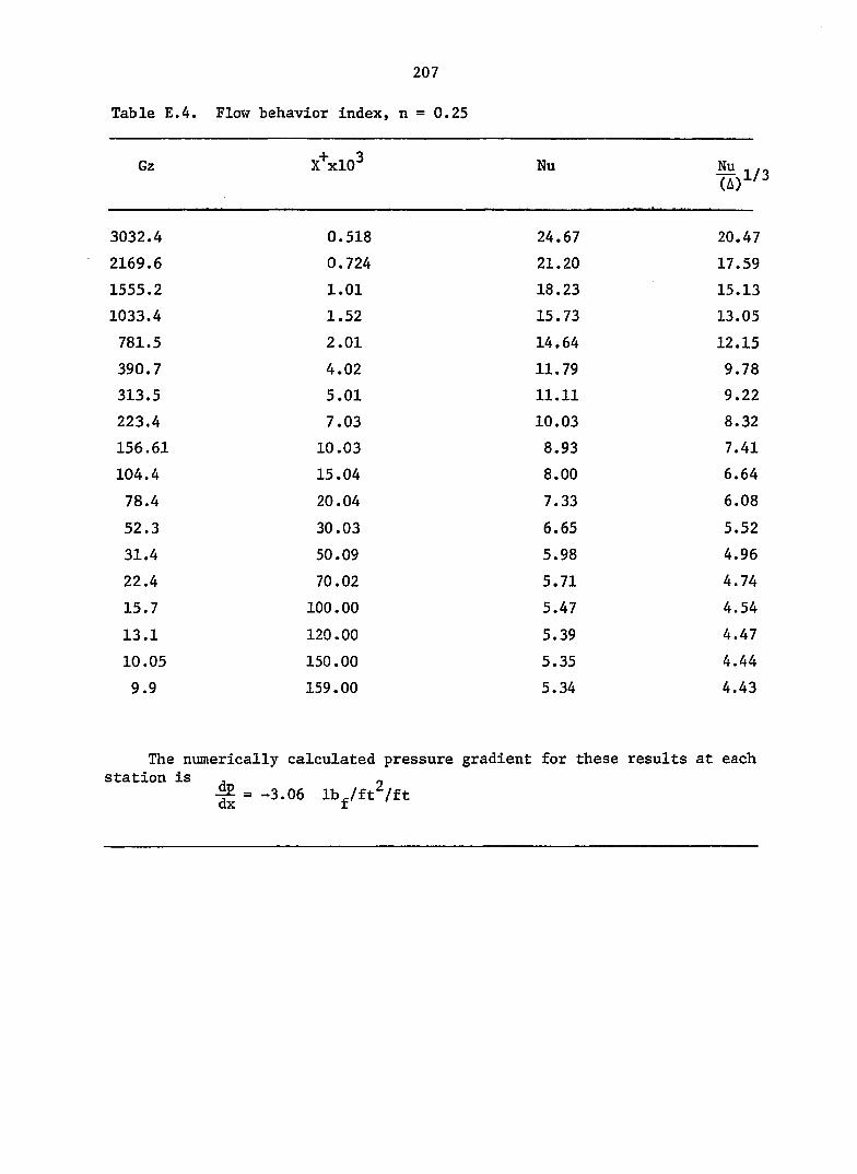
207
Table E.4. Flow behavior index, n = 0.25
Gz X^xlO^ Nu Nu ... (a)l/3
3032.4 0.518 24.67 20.47
2169.6 0.724 21.20 17.59
1555.2 1.01 18.23 15.13
1033.4 1.52 15.73 13.05
781.5 2.01 14.64 12.15
390.7 4.02 11.79 9.78
313.5 5.01 11.11 9.22
223.4 7.03 10.03 8.32
156.61 10.03 8.93 7.41
104.4 15.04 8.00 6.64
78.4 20.04 7.33 6.08
52.3 30.03 6.65 5.52
31.4 50.09 5.98 4.96
22.4 70.02 5.71 4.74
15.7 100.00 5.47 4.54
13.1 120.00 5.39 4.47
10.05 150.00 5.35 4.44
9.9 159.00 5.34 4.43
The numerically calculated pressure gradient for these results at each station is , _
^ = -3.06 Ibg/ft^/ft

208
appendix f: analysis of fully developed newtonian heat transfer
This appendix outlines a numerical scheme to predict Nusselt number
for a fully developed Newtonian flow with temperature-dependent
viscosity.
Numerous highly viscous Newtonian fluids such as lubricating oils,
transformer oils, etc. are commonly used in industry. In these fluids,
viscosity exhibits a strong temperature-dependence. This viscosity
variation has a strong influence on the heat transfer rates at the
wall. Free convection arising due to temperature-dependent density is
small for the highly viscous liquids.
In the fully developed case, the local velocity and temperature
profile does undergo changes due to temperature-dependent y; however,
these changes are small and can be neglected. The temperature
difference (t^ - t^) is constant and flow can be considered to be
"locally fully developed."
Problem Formulation
Statement of the problem
The purpose of this analysis is to investigate Nusselt number for a
laminar flow of Newtonian fluid inside a circular tube subjected to a
uniform wall heat flux boundary condition. The fluid velocity and
temperature profiles are fully developed. All the fluid properties
excluding y are assumed to be independent of temperature. Since the
majority of the fluids under consideration exhibit an exponential

209
viscosity-temperature dependence, the following relation is selected:
y = a exp (-bt) (F. l)
Governing equations
The equations are formulated subject to the following assumptions
1) fully developed velocity and temperature profiles,
2) negligible axial conduction and viscous dissipation, and
3) all fluid properties other than u are constant.
With these assumptions, the momentum and energy equations are
reduced to
c dx
dx~ r (F.3) ^ b _:k 3_ , at.
and boundary conditions are
• "c ' 'v " ° ° "
Equations (F.2) and (F.3) are rewritten in nondimensionalized
form as
and

210
where
a exp (-bt) y =
and boundary conditions are
i - " » = • " . ( # c = =
(ai'c ° 0
Other nondimensionalized parameters are defined in the list of
nomenclature.
These two equations can be integrated by an iterative procedure in
which the temperature distribution for constant properties is used as a
first approximation. Then using the prescribed ji-t variation, the
momentum equation is integrated numerically to yield a second approximation
for the velocity distribution. This velocity distribution is employed in
a numerical integration of the energy equation to yield a second
approximation for the temperature distribution. The procedure is
repeated until the velocity and temperature distributions do not change.
Then the mean velocity, bulk temperature, etc. are calculated.
Integral equations
Equation (F.4) was integrated twice, and the constants were
evaluated using the nondimensional boundary condition, which results in
the following integral form;

211
R.
1 dp/ r 2 dx( J # dR (F.6)
The integral form of Eq. (F.5) is
R
T. = + ? e.
R. R.
/'s (/'•>•' dR dR ( F . 7 )
Since there are two equations and three unknowns, velocity,
temperature, and pressure, one more equation is needed to solve this
problem. The third equation is obtained from global continuity:
m = ^^pudA (F.8)
A
which can be written in nondimensional form as
R w
/ yd' m = 2 7 T P J R . U j d R ( F . 9 )
0
Now, Uj is given by Eq. (F.6) so that Eq. (F.9) can be solved
explicitly for dP/dX:
/ rj
/ ) ^ = (m/pTT)/ I J R, I / (R^/yJdR I dR [ (F.IO)

212
Method of Solution
Equations (F.6), (F.7), and (F.IO) were solved iteratively. A
uniform grid spacing along the tube was utilized to accomplish the
numerical integration depicted in Fig, F.1. Simpson's rule was used
for numerical integration. The flow chart of the numerical procedure
is shown in Fig. F.2. Subscripts 1 and 2 are used to denote values of
1st and 2nd iteration steps. An iteration by a shooting method was
employed at various steps to correctly predict appropriate temperature
at the tube centerline so that (8T/3R)^ = 0 and, near the wall
k(dT/dR)^ = Q^. The bulk temperature was computed as
/"
/""ujr.de
0 *
From this, the Nusselt number, (y/y^), wall temperature, etc. were
computed.
Computer code for this analysis is given at the end of this
appendix.
Results and Discussion
In this analysis, results were obtained for various values of heat
fluxes. The predictions are obtained for several viscosity ratios up
to = C, and these predictions are tabulated in Table F.l.
In Fig. 4.7, predictions of Nu^ are plotted against X"*", for X"*" >1x10"^.

213
1 -
2
3
j-1
j
j+1
N-1
CENTERLINE
WALL
Fig. F.l The finite-difference grid for fully developed flow inside a circular tube.

214
INPUT-tg, q"^, u. D.Wg
CALCULATE, CONSTANT PROPERTY
"l,J ' 1 ,j (dp/dx)^
NON-DIMENSIONLIZE ALL PARAMETERS
I CALCULATE j FROM T^ .
+
CALCULATE L^.j andj^j^ '[f];
let tg = t ^ , calculate tg j
i CHECK (|I)c - 0 and ^
NO
ASSUME DIFFERENT T 1.1
YES
CALCULATE , MAX | U, . - U, . = DU I * »J I
MAX I T, . - T, . I = DT i ^ >j l*j i
CHECK IF DU AND DT ARE SMALLER THAN CONVERGENCE CRITERION.
NO
CALCULATE ^
CHANGE ( )2,j . ('
YES
calculate tj^. t^.
Nu etc.
3= STOP
Fig. F 2 A flow chart of the computer program.

215
Table F.l. The Newtonian fully developed predictions
Btu/hrftZ y AT W/W* Nu WUcp
250.0 1.18 1.65 4.69 1.08
500.0 2.35 2.58 4.97 1.14
750.0 3.53 3.87 5.22 1.20
800.0 3.77 3.98 5.29 1.21
850.0 4.00 4.5 1 5 . 31 1.23
1200.0 5.65 7.55 5.59 1.28
In Fig. 4.10, a log-linear relationship is seen between (Nu/Nu^p)^^ and
(li/y^) . The slope of this log-linear plot is 0.14. Hence,
(r). - cp/m»)"" (f.12) cp
and m = 0.14
Yang [32] and Deissler [33] have performed a similar analysis. Yang
has obtained m = 0.11 while Deissler has computed m = 0.14. Thus, the
present analysis is in excellent agreement with Deissler's prediction,
and does not differ significantly from Yang's predictions. Shannon and
Depew [34] have shown that for U/]\, < 5, Eq. (F.12) holds, and for
y/y^ > 5, (Nu/Nu^p)^ has an asymptotic value of 1.5. No such
asymptotic relation was found in the present analysis.
The predictions of all the analyses described so far are of the

216
form as given in Eq. (F.12). For a constant wall heat flux boundary
condition, t^ is unknown and, hence, an iterative procedure needs to be
followed to estimate y and Nu . To avoid this iteration, a new W 00
parameter yAT was introduced as
-^(b) 2k
For a known fluid and q^, yAT is calculated explicitly. A plot of
(Nu/Nugp)^ against yAT is shown in Fig. 4.13 and this curve is
correlated as
= 10 + 0.069 yAT - 0.0033 (yAT)? (4.14) nucp
With this correlation, (Nu/Nu^p)oo is computed explicitly. Thus,
iterations are avoided and the design procedure is greatly simplified.
Computer code
In this section a computer code utilized for the fully developed
Newtonian analysis is given.

217
c c c c c c c c c c c
T U S P B C G P A M I S O E V E L C P Ê O T O S O L V E T H E F U L L Y O E V E L O P E O N E I l T C N l A N F L C W I N S t O L A C I K t L L A k T U B E . S U E J E C T t O T O T H E C O N S T A N T W A L L H E A T F L U X 8 C L N C A H Y C O N D I T I C N , T H E D I S T A N C E L F R C P T H r I h L E T O F
N J S S E L T N U M B E R I S O E S I E N E O T H E t - d A T E O T U B E
A T ( H E
I N T H I S K k U G R A M V I S C O S I T Y P B C P E F T Y
I S T H E C N L V T E M P E R A T U R E O E P E N D E N T F L U I D
T H I S P P O U I C M I S S U L V F C B Y T H E
E N E R G Y E U U A T I l h
I T E R A T I O N O F I H E ^ O M E N T U M A N D
C C c c c c c c c c c c c c c c c-c c c c c
AC
A S L N Y qu XM
C f i C S S - S e C T I C N A L
S U R F A C E A R E A C F L u f t C T H F T N U M B E R < N L S T B E H A L L H E A T F L J X PASS FLC* HATE
A R E A O F T H E
T H E T U 8 E
TUBE
E V E N i O F Y G R I D 8 T U / H R / F T / F T
F T * F T F T $ F T
S P A C E S I N T H E T U B E
F O L L C k I N G Q U A N T I T I E S ARE E V A L U A T E D A T T H E I N L E T C F T H E T U B E
cpo 00
H T K O T O X V O
S P E C I F I C M E A T B T U / L B M / F D E N S I T Y L B N / F T / F T / F T T H E R M A L C C h O U C T I V I T Y B T U / H R / F T / F T c M P E R A T L R E F ( R A N K I N )
V I S C C S I T L H M / F T / S E C
1002 1 0 0 3
1 0 0 4 C
* * * * * * * * * M A I N P R C C . R A M * * * * * * * * *
O I M E N S I C N T ( 1 0 1 . 2 ) . S U M ( 1 0 1 ) , S U M U P ( 1 0 2 ) . D I F T I l O l ) , C < 1 0 1 ) ,
I S U N H d O l ) . C 1 F U ( 1 0 1 I C O f M C N / V E L / E V ( I 0 1 ) . U ( 1 0 1 , 2 I . R ( 1 0 1 ) . D E L Y . O P O X . N . X M A S S . P l C C M M C N / S H L T / X ( 2 0 ) . Y ( 2 0 ) , X R , I
C C k N C N / S H L B / X E ( 2 0 ) t V B ( 2 0 ) . X R B . I T B
R E A L L R E A D ( 5 , 1 0 0 2 ) 0 0 * X V O . U O . C P O , T O . R A O R E A D ( 5 . 1 0 0 3 . t N O = e O C ) Q k . L . H T K O . N V
W R I T E ( e , 1 0 0 2 ) O O . X V O . L O . C P O . T O . R A D W P I T E ( C . 1 0 0 3 ) C h . L . H T K O . N Y F C P V A T ( 6 G 1 2 . 6 ) F C P y A T ( 2 F I 0 . 2 . F l C . é , I 5 > G C C N = 3 2 . 2 P l - ^ . 1 4 ( 2
X J C C N V = 7 7 8 . 2 6 C K £ = 1 . 1 C T S = 0 . C 5 C L f C — 0 . Z A £ = c . 0 4 P I $ H A D * L A C = P 1 * R A C * K A D X M = C O * U O * A C
T M = ( G k * A S / X y / C P O / 3 e O O . ) + T O D T C X = 2 . 0 * P l * 0 W * R A D / X M / C P 0 / 3 6 0 0 .
W P t r E ( e . l 0 0 4 ) X M . T K . O T O X F C P M A T ( ' O ' . S X , ' X * V = ' , F 1 0 . 4 . b X ,*TeULK=' * F 1 0 . 3 . 6 X t * O T O X s • . F t 0 . 4 )

A n A A A A O r M r *D
I O O y m z r -
m m < m C > €\ *0 o > o z X T 7! X 2 m c n r n
n 7 1 n n z T . H 1 1 n i l < m < •n % r n r T m > w t f . O I I H I I r Tl fh T J r - r * 0 n > »• O •n (n •n m C A < z n o z O O X "0 r 23 « M M A m Z 1 # c > o m O o w * M 71 O Ui o c X z O m X c o X m r 70 I I o M > < O c m (A r m o -4 n o r r w I ir» r r Z * < N, • m o 71 m o T) o < H T o V ( A o v P 2 o n c M I I C Z # s. o Z m V c o < c o T r O c z c o O 2 U l z <
X H C r i s >
r • V
o w \ c o
N « m O r n X
z CD m ( A < X
* 0 o
e r c < n z < B r z H N *
> # r Tl
Tï O
-4 U
> Z O
V (A • 4 m % n m
# w H I t
• O T ) * 0 C A ( / ) ( A O A m
I l I I S ( i i
• V i n O s. m o r m
o u o
M i/i •n m. o X I O f) m Z z II T3
Tï a r e\ O T z M n 9 X M > m II \ t l
I I r o 1 •n A 1 m
o O o w « T o
Ul o S I * X u I * <
o w Tî o % > 1 (A
z X o O O 1 A c X o N » o •D T • 4 il o O H *
A X % m m O *
Tî X z & C C D M M O
H X X w > 2 c
Ct Z C A U) K o C X U z
XI o ui » H 5
o O O > " 4 •Q < O O r m > X <
X ; T H <
3 > O
(m O 2}
tl m Tl lA
o H c è S r w 71 •4
H C A
•n N m N •n X m • e #
s c s i
o o
o ro o
o o
r) o
A > 7) c 7 1 % M. Tï m c A - 4 A C o A X X X r A a r\ 71 71 n 71 A n I I A N A T » t) 7 1 z T c H C . W n H I I r 2 H X H *• " M X r o ? n • g Ci r m > m m m A • M o 1 A 9 > « 4 M Z 4 1 - V « n X « 4 ftv a A M Tl U L. A * n o m A r o 1 1 « T) O c A O O * t. r* O r X z o o o # 1 * «-
A ro o X * c Z X A » OD 5 o r s > ïi Û O O 7 1 O O o * « 4*. O O O X X X T ! w m r m T X 7) W «4 r 4 o • 4 A m • A M # A 1 o X 7 1 C A If) C. m c « O O fn Tt «* 7) V X X C * 0 m 1 I r u 71 %) m r L. H > m z c A X O C > c. A * o X o il H I i 4» X c Z w G M -4 X o o » < C •D Z T Z (.
1 O X ro o ro * s
( A z > l A #4 o «4 X c. X X) X
m s > S c 71 o c M > «4 o
O N O z X Z « >
« o X
n o z fa H > Z
*0 !n c tï m n
tj 71 o m r m (/)
A 3 o o O z Z z z A o m m m z r * I I Z r A I I * il i l z #4 < •< z fi z Z «f II o il 1 Z 1 1
Z 11 X o 1 I V i A C. o % A. m ïï m o
r X •c z
« z 4» < n ru m r i/
a n
u) m
z a
% m < i a T)
tf) *0 > o z Çi
n5 m 00

219
c A S I M I L A R F C L Y h C M I A L A N C L I N E A R F I T I S C B T A I N E D F O R T H E O T / O V
C O T C v e = F S A * T ( N . 1 ) « P S B * T ( N L « l * * P S C * T ( h K . l ) + P S O * T ( N 8 « 1 ) O T O \ L - ( T ( K L * 1 I - T ( k , l ) ) / D E L V I P E R = < U T D Y P - O T D Y L I * 1 0 0 . / O T D Y P H R I T E ( 6 . 1 3 â O ) O T C V F t O T O V L t P E R
1 0 5 0 F C K P f T { « 0 = • « O T C V P s » , F 1 0 . 3 . ' F / F T ' » 5 % . ' D T D V L = ' . F 1 0 . 3 . ' F / F T ' , S X , *
l P E P C E h T A G E = ' , F 1 0 . 2 )
C C C C N V E R S I C N F A C T O R S F O R N O N - D l M E N S I C N A L I Z I h G
C OCCNV-CO xvccnv=)(xo U C C h V = L O x c c N v = > v o / o o / u o pccnv=do•uc*uo/gcc^ X K C C N V - X V 0 4 X V O / C O / I . O T C C N V = t O » U O / G C C N / X J C C N V / C P O C F C C h V = C F O
X K C C N V = 3 6 0 0 . « X V O * C F O X R f C = R f O / X C C N V W R I T £ ( e > 1 0 6 0 ) C C C N V . X V C C N V . U C G N V . X C C h V . P C O N V « X M C O N V « T C O N V . C P C U N V *
1 X K C C A t . X R A C 1 0 6 0 F O R M A T ( " O " , S X . • O C C K V = * . 0 1 3 . S . 5 X , • X V C C N V = * , G 1 3 . S . 5 X . ' U C 0 N V = « . G 1 3 . S ,
1 S X . ' X C C N V = ' , G 1 3 . 5 , I S X , ' P C C N V = ' , G 1 3 . E , / . 5 X , « X M C C N V = ' . G 1 2 . S , S X e « T C 0 N V = ' « G 1 3 a 5 « 5 X * • C P C O N l V ' , G 1 2 . S . 5 X , ' X K C C h V = ' , G 1 3 . 5 , 5 X . « X H A D = ' « G 1 3 . S i
C C C A L C U L A T I C h C F THE T E M P E R A T U R E D E P E N D E N T V I S C O S I T Y
C OC 40 W-LSN T - = I < J . I J e v < j ) = v i s c ( T J ) / x v o T ( J , l ) = T ( J . i ) / T C C K t
( J ( J . 1 ) = L ( J . 1 ) / L C L r V R < J ) = P ( J > y X C C N V
4 0 C C A T I N L E X M A S 5 = X M / X V C C N V
D E L Y - D Ê L V / X C C N V
L C C F = C P B S T = C . 0 I T E G T = C L I = C
I T e - 0 P B E T - C . O
C C C A L C U L A T I O N C F V E L C C I T V P R O F I L E
C C A L L t V E L
C DC SE J - I«NT2
50 0 ( J ) -U (J . 2 ) «UCCNV WKITL (6 ,10 10) M f t l T E i £ • 1 I C C ) ( C ( J ) * J = 1 , N . 2 )
U r R I T E ( £ . 1 1 0 E ) 1 1 0 5 F C P M A T < • 0 * t 2 0 X . • • » 4 C O M P U T A n C N A L L C C P B E G I N S * * * « )
C C S l ^ P S C N S f - U - E C F I N T Ê C f i A T I O N F O R T b E C A L C U L A T I O N O F M A S S F L O W C
140 SUVCL)=0 .0

220
oc ISO J=J.N,2 SUM(JI=SLM(J-2)+(DELV*(U<J-2.2)*m(J-2)*4.»U(j- l ,2**R<J-l lu(j.z))/3.0>
SLW(J-ir=<SLM(j)*slk<j-2*)/2a0 ISO CCNTINCE
XP1=SLP<131)*XCChV*XCChV*UC0NV$00*2.*PI CMC^AbSi<**l-XM)$lCO.O/XMj IF (CMC.CE.S.0) GC TO 69»
C C TEMPERATURE CALCLLATICN c
ccaxkcc^v*otdx*xcc^v/tconv/htko C ASSUME CENTEKLIKE TEMPENATtHE T<1,2) C tASED CN This CCMPLTE T(J,2*
Tl l f£> = T( 1.1 ) SLMUP<1)=0.0 SUMIP( 2 )^^<DELt /3 .CI*( (4 .*SUM(2) /R(2»)* (SLN<3) /m(3) )** r i 2 , 2 i - 7(1,2)»5LMIP(3}*C0 T(c.Z)-(T(1.2)«T<3.2i) /2. OC 20C J-5,N,2 SUMUP(J) = SUMUP<J-2)+(((SUM(J-2)/R(J-2)) + (4.*SUM(J-l) /R(J-1 ))
#<CELY/3.)) T1J,2)=T(l .Z)*5LMLP(J)*C0 1< J-1. 2)=(T< J-2.2 MT( J,2) ) /2.0
£00 CCMINLE C CHECK T^AI ThE SLOPE CF THE TEMPERATURE PRCFILE IS ZERC AT THE C CEhrEPCINt CF Tl-E TUEE
OTOY2= TCLhV*(T(k,2)*PSA+T(NL,2)*PSB+T(NK,2)$PSC+T(NB#2)*PSO) TC=(DTCVP-DTOY2)/DTDyP TOR=AE<<10) SC=(T(1.2)-T(j .<))*100./T<l,2l SC1=AES(SC) DO 2bO J=l,h,2
250 0(J)=T<J.2)*TCChV NF>1TE(C. 1020) V«RlTE(é»S10a) (C(J)« J=1,N,2) TC=T<1 .2>«TCCNV 1F((SC1.LE.CTS>.AhC.(TON.LE.CWS)> PRST=1.0 IF (PPST.GE.1.0) CÇ TC 300
300 ITERT-ITERT+1 l - ITEFl V(I)=TC X( l )=TC *RITC(t,1110) lTEKT.SC,DTOY2,TO,TC,PRST,LCOP,XMl
1110 FORMAT <•0*.SX. ' ITERAriCN='. IS.IOX.•(DT/OY) C£NT=* ,G13.5.SX.*(0T/0Y 1) *ALL='.G13.3.SX,/.SX. ' MALL SLCPE DifF='.G13.3,5X,*NE* TC=',F10. 13.SX. 'PRST=',F10.3,SX. 'LOOP='•1S.2X. 'XM1=*,F10.5) IF(PRSl.GE.l) GO TC 350 tkF ITECe. 1010)
C c CCMPUTE ThE TEMPERATURE DIFFERENCE BEThEEN TWO CONSECUTIVE C TEMPERATURE PRCFILES C
OC 310 J=1 .N.4 OIFT<J) = (T< v,2)-T(J. l ))*TCCNV
310 CCNTINCE WRITE(£«1120)
1120 FCRWAT('0' ,SX.«**ClFT(j ;***) NRITE(e.1100) (01F1IJ)•Jxl•N.4)

221
C U P C A T E T h E V A R I A B L E S
C D C 3 3 0 J = 1 . h T ( J.n= T ( J . Z I
3 2 0 C C M I N C E 1 F < I T E R T . G E . 2 0 ) G C T O 6 9 9 I F ( L C C P . C E . 3 0 > G C T O 6 9 9 1 F < I . G E . 2 ) G O T O 3 c S T ( 1 « 1 ) = ( T ( X * 1 > * T C C K V - 1 C . 0 ) / T C C N V G C T C 1 4 0
3 3 5 X T = T C
C C t S E T h E S H C C T I N G M E T h C C T C C O R R E C T L Y G U E S S T H E C E N T E R L I N E T E M P E R A T U R E C T H I S I S C C K E C N L V A F 7 E F T H E S C C N D I T E R A T I O N
C C A L L S H C O T
C T ( l . U = X R / T C L N V X C = A E S ( ( X R - X T ) * 1 0 0 . / X R » I F ( X C . L E . 0 . 5 C ) P R S T = l .
I F ( P R S T . G E . l . ) G C T O 3 5 0 G C T C 1 4 0
3 5 0 D C 4 C C J = l « h , 2 0 I F T ( J ) = ( T ( J . 2 ) - T ( J . l ) } • T C C i N V
4 0 0 C C h T l h L E tiRITE(CtllEC)
C C V A R I F V T H A T T H E S L C F E C F T H E T E M P É R A T U R E P R O ? I L E A T T H E T U B E C E N T R E C I S Z E R C A N C T H E D I F F E R E N C E H E k T E E N T * 0 C C N S E C b T I V E T E M P E R A T U R E C P R O F I L E S I S V E R V S K A L L C T h i s C C N F I R M S T H A T T H E T E M P E R A T U R E P R O F I L E I S O . K . C
1 1 5 0 F C K P f T I " ' , 5 X , ' * $ T E M P & H A T U W E P R O F I L E O . K . * * ' « / ) W P I T E i e . l l Z O ) W R I T E ( C . l l O O ) < 0 I F T ( J ) . J = 1 . N . 2 I
C C S I M P S C K S f L U L E C F I N T E C F A T I C N T O C O M P U T E B U L K T E M P . T 8
C S C N H = 0 . 0 D C 4 £ 0 K = I . K L . Z J = < h - K ) + l
S C P H = S C M H » ( C E L Y * ( T ( J - 2 . 2 ) $ U ( J - 2 , 2 1 • R ( J - 2 ) • 4 . » U < J - 1 . 2 ) * T ( J - 1 * 2 ) * R < l J - l ) # U ( J . 2 ) * T ( J . Z ) « R ( J ) ) / j . O I
4 £ 0 C C M I K L E T B - 2 . 0 * S C M H * T C C N V / ) < R A D / X R A O
C C C A L C U L A T I O N CF T H E H E A T T R A N S F E R P A R A M E T E R S C
T I » 1 = T ( N • 2 ) « T C C N V 0 E L T A = T * 1 - T E H l = C k / D E L T A X N U C = F l * 2 . * P A 0 / h * K C
W R I T E ( e . 1 2 0 C ) T h I . T B . O E L T A . H l t X N t O 1 2 0 0 F C R M A T ( " C ' . S X , • T h l = * . F i 0 . 2 , 5 X , ' T B = * , F 1 0 . 2 , S % . * D E L T A = * , F 1 0 . 2 , S X .
l ' H l = ' . F 1 0 . 3 , ' 8 T L / H R / F T / F ' . 5 X . * h U O = • . F 1 0 . 3 > P R = 3 6 0 C . * V I S C ( T e ) * C P 0 / H T K 0 R E = C O * Z . O * R A D * U O / V I S C < T B » G / = 3 6 0 C . C * X M * C P O / H 1 K O / L
VRATI=VISC(tb)/vi ;C<mit

222
P C = O F C X « P C C N V / X C C N V W K I T E i C . 1 2 3 0 } R E . G 2 . P R . V R A T I . P 0
1 2 3 0 F C H M A T < ' 0 ' . 5 X , * R E C = « , F 1 0 . 3 . 5 X . ' G Z = ' . F 1 0 . 3 « S * . * P R = * . F 1 0 . 3 . I S X . ' V I £ C R A T I C = * . F 1 0 . 3 * 5 X . * O P O X - * . F 1 0 . 4 ) 0 0 4 7 C J - l . N T ( J . l ) = T ( J . 2 )
U < w • I ) - 0 < J . 2 i T J = T < J . 1 ) * T C O N V E V < J J = V I S C < T J ) / J > V C
4 7 0 C C N T I N L E C C C M E C K I k G T H : C A L C U L A T E C B U L K T E M P E H A T U R E W I T H C O M P U T E D B U L K T E M P E R A T U -C R E F O P A G I V E N K A L L M E A T F L U X C W . A N D L E N G T H L F f i C M T H E I N L E T
C OTC=At£(ÎE-TM) I F i c r e . L E . O . 5 ) G C T C 1 2 4 5 ITE'ITU+l I F ( I T e . G E . 5 ) G C T C 6 9 9
I F ( I 7 B . G E . 2 ) C C 1 0 4 7 5 X B ( 1 l - T ( 1 , 1 ) « T t C N V Ya< 1) = T E - T *
wkite(e. 1238) vedt.xbcn 123a F C B M A K'O* .2X ,• Tfc-TM=« , F10. ? . 2 X,»T CENTRE= • • F 10 . 2 >
T « l . l ) = ( X a ( I ) + 1 2 . I / T C C N V
C C 1 C 1 4 0 « 7 3 V E H T e > = T E - T M
X f ( i 7 8 ) - T ( 1 , l ) * T C C h V xie^xe(its) * H I T & < ( , 3 0 0 C j > E ( 1 I B ) « X T B » I T 6
30 0 0 F C H M A T ( • 0 ' . 2 X , • re - T M = « . F 1 0 . ; > i 2 X , • T C E N T « E = « , F 1 0 . 2 , 2 X , * I T E R A T I O N F O R 1 T h E e U L K T E M f = » s I 5 )
C C L S E O F S H G C T I N G M E T H O D T O O B T A I N C C R W C C I G U E S S F O R T H E C E N T R E L I N E C T E M F C k A T J K E S O T H A T C C B H E C T B U L K T E M P E R A T U R E I S C H T A I N E t )
C C 4 L L S h L i a X C E = A B S ( ( X T E - X K E ) * I 0 0 . / X R 8 )
I F ( X C 6 . L E . 0 . 5 . A N D . C T B . L E . 0 . 5 > P U S T - 1 W R I T £ ( e . 4 0 0 0 ) X R E . > C B , P 8 S T
4 C O O F O R M A I ( " 0 * , 2 X « * X K B = « , F 1 0 . 2 , 2 X , ' X C B = ' . F I 0 . 2 . 2 X , • P B S T = • . F 1 0 . 2 )
I F ( P E 6 T . C E . 1 ) G C T O 1 2 4 5 r ( 1 . 1 ) = X K d / T C C N V E f - P = X t £ - X R B * R I T E ( 6 , 1 2 e 9 ) l I B t t R R
1 2 3 9 F C f . M A T t ' 0 » , S X , • I T C k A T I U N = ' , I % . S X . « T B - T M = ' . F 1 0 . 2 )
C C T C 1 4 0 C C h I T h N E h T E M P E R A T U R E . C O M P U T E N E » V I S C O S I T Y A N O , H E N C E . N E W V E L O C I T Y
C 1 2 4 5 V K = V I S ( ( T B )
U F C X = - 6 . * V 8 # U 0 / G C C r / R A D / R A D D P D X = D P D * * X C C N V / P C C N V
C C A L L L V L L
C C B S = 0 . 0
c C C H E C K T F E D I F F E R E N C E B E K T E E N T W O C O N S E C U T I V E V E L O C I T Y P R O F I L E S C I F T H E D I F F E R E N C E I S S h A L L T A K E T H E P R I N T C U T
C
o
n c o T l.
1
7 #
C M m ii r
l. r o + c
q3 o
ru o
C o n l «
r u o
n (n w r # « z r • i» i\)
ro H M
n w + n c en 7 z r -4 "O % z C :
m i w
% »
vç ru ro
h ) o
N N
— u> r
t) m. m #. X o N IN) • « V
( A L C ^ 3L *0
0) o c n z * n r o
o
7 îr Là C « z z d • ^ t o
I ro
U) &n r r % t - n ( -
I l n c / > n n 7 ^ 7
c • il r w w ^ X lA « r* Il H a C II m o < z # " • tA • C • o -k z y
X X
(n c
c I
(V)
o m r
u
N t fV (A • C O z
c
I l\)
« 7}
I f» + »
* O) c X c
c . I
# X
o o o o
o (A (A L . o (A T! m •tî C O A r 71 r I l n 7 r m X n Tl n z z Z r t T » r\ t z c c 1 II r T - 4 Z H m z
z ; e n Z > m > m z n X \ T • o 1 H H (A z * m + ro f% X < t u II C <
X o r u O f u z m II L _ U 11 o o r <A o o o CA s w C Q r m c z z O O z < & c r C X c c Ul
X f u l U m o o e o * f f i z
* c (A (A o C C m O < z r m (A r < (_ o
» II < y n O * r f u fo X Z o
A u t u (A X
s 1 -4 C ru
m <
V tu
+
» c I
s m <
V
p r c* *0
o X
« * m <
z • -T» O
O • •- O -p
<
o V o X
X z > (T. (A
A n (A
Z *0 (A n z (A
A > tA r r n m c~ tj
n z z m (A n c ( A < m m o r
O •n A n w X M
< M
Z H m o X >
m o o O O
m ( A Ci Pm m o z m • n T X o O l _
• o • H - 4 O " D X m I I
X X r ( A f m m % H H L .
Ci A t u m m o
o * C A A
n Z % r < z - 4 u n I I r H V r + I I
H
r z H
r u W
o f m X
s -h A m o
n% L. # I l ^ #" û
z o tu
a o o
tu ut o
(n o o
S g Ci M r c m c M A M C o o s Tl n "n n X A Tl A " H A
m 2) Z r TJ -* •H •4 • n M z M A I I C ( t t m m n r I I m > m X O n O
o r H (A Z c O m» n » A A A r C y[ X n r m C 1 1 u
O X m A u t u et + r u m c c o ( n m O e n A o o o o c A c_ z
CE
* *
o X (A N t u
O o O A 1
• n O O C m Ci Tl r f- A r- #4 r u
c . O I I l. M c A
C « e- X « o «A
C o
I I C C C I I n
% 0 D Z z
z < l u
o o
n3 tsd W
n z
o

224
u(k.2)=0«0 * K I T E < ( . 2 0 C 4 *
2 0 0 4 F C R M A T ( * 0 « . S X . ' C t T O F V E L O C I T Y L O C P ' * reilpn E N D
C c
S L E R C L T I N E S H L T B C S H O C T l k G M E T M C O F O R T l - E B U L K T E M P E R A T U R E C
C C M M C N / S H U B / X E < 2 0 ) • Y U ( 2 0 ) . X H B . I T B I T = I T 6 - l SLE=( YB(lT)-YE(lTE)>/(XB(ITi-Xa(XTB)> XRE-XE (1TB>-CYE ( ETO/SLB) be7lsn end
C c C S H O C T I N G M E T H O D F O R T h E C E N T R E L I N E T E M E R A T U R E
S L E C C U T I N E S H C C T C
C C M N C N / S H U T / X ( 2 0 ) . Y < 2 0 ) . X H . I I L = I - l S L = ( Y < I L > - * ( I L ) ) S L = ( Y ( I L ) - V ( 1 > 1 / ( X ( I L > - X ( I ) > X R = X < l L > - < Y i I L ) / S L )
R E T L R N E N D
c c C F L U I D V I S C O S I T Y - T E P F E R A T U R E OBPENEthCB C c
F L N C T I C N V I S C ( I ) C U N I T S l . B M / F T / S E C
D A T A X I , X 2 / 0 . 2 4 5 2 4 6 - 0 2 . - 0 . 1 9 7 2 2 E - 0 1 / E T A = T - 4 6 0 . V I S I = 3 2 . 2 * X 1 * E X P ( X Z # E T A ) RETURN end

225
APPENDIX G; VARIABLE PROPERTY NUMERICAL PREDICTIONS
In this appendix, variable property numerical predictions are
tabulated. The predictions are obtained for
1) Constant wall heat flux boundary condition
2) Hydrodynamically developed and thermally developing flow
3) All fluid properties, other than K and p, were assumed
to be independent of temperature.
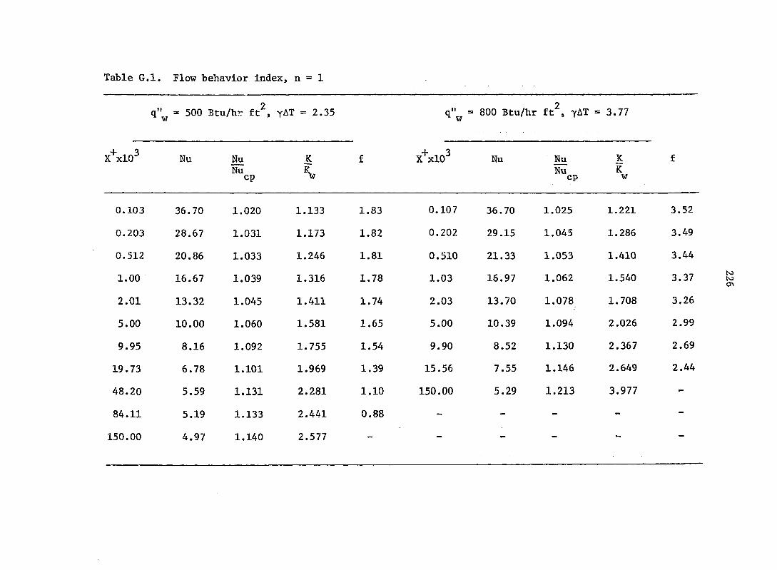
Table G.l. Flow behavior index, n = 1
4"w 2
= 500 Btu/hr ft , YAT = 2.35 Q"w = 800 Btu/hr ft^, "yAT = 3.77
f X'^'xlO^ Nu
PU
K
\
f X^xlO^ Nu Nu Nu cp
K K w
f
0.103 36.70 1.020 1.133 1.83 0.107 36.70 1.025 1.221 3.52
0.203 28.67 1.031 1.173 1.82 0.202 29.15 1.045 1.286 3.49
0.512 20.86 1.033 1.246 1.81 0.510 21.33 1.053 1.410 3.44
1.00 16.67 1.039 1.316 1.78 1.03 16.97 1.062 1.540 3.37
2.01 13.32 1.045 1.411 1.74 2.03 13.70 1.078 1.708 3.26
5.00 10.00 1.060 1.581 1.65 5.00 10.39 1.094 2.026 2.99
9.95 8.16 1.092 1.755 1.54 9.90 8.52 1.130 2.367 2.69
19.73 6.78 1.101 1.969 1.39 15.56 7.55 1.146 2.649 2.44
48.20 5.59 1.131 2.281 1.10 150.00 5.29 1.213 3.977 -
84.11 5.19 1.133 2.441 0.88 - - - - -
150.00 4.97 1.140 2.577 ». — — -

Table G.2. Flow behavior index, n = 0.75
q"^ = 1000 Btu/hr ft^, yAT = 1.34
+ 3 X xlO Nu Nu
Ku cp
K K w
f
0.104 37.85 1.007 1.0754 11.05
0.200 29.65 1.012 1.097 11.03
0.506 21.52 1.020 1.137 10.95
1.01 17.04 1.042 1.175 10.86
2.01 13.61 1.054 1.224 10.73
5.01 10.18 1.062 1.310 10.38
10.04 8.27 1.080 1.394 9.95
20.14 6.46 1.088 1.527 9.34
50.61 5.58 1.096 1.629 8.14
102.30 5.10 1.099 1.696 6.88
150.00 5.00 1.111 6.63
q"'^ = 2000 Btu/hr ft^, yAT = 2.62
+ 3 X xlO Nu Nu
Nu cp
K K w
f
0.1050 38.66 1.030 1.153 10.95
0.202 30.35 1.038 1.199 10.87
0.508 22.15 1.051 1.282 10.71
1.02 17.66 1.080 1.366 10.54
2.02 14.20 1.102 1.473 10.30
5.02 10.69 1.117 1,672 9.65
10.08 8.75 1.145 1.871 8.91
20.22 7.25 1.155 2.123 7.88
51.20 5.94 1.172 2.475 6.08
104.40 5.44 1.172 2.636 4.46
150.00 5.33 1.184 _ 3.91
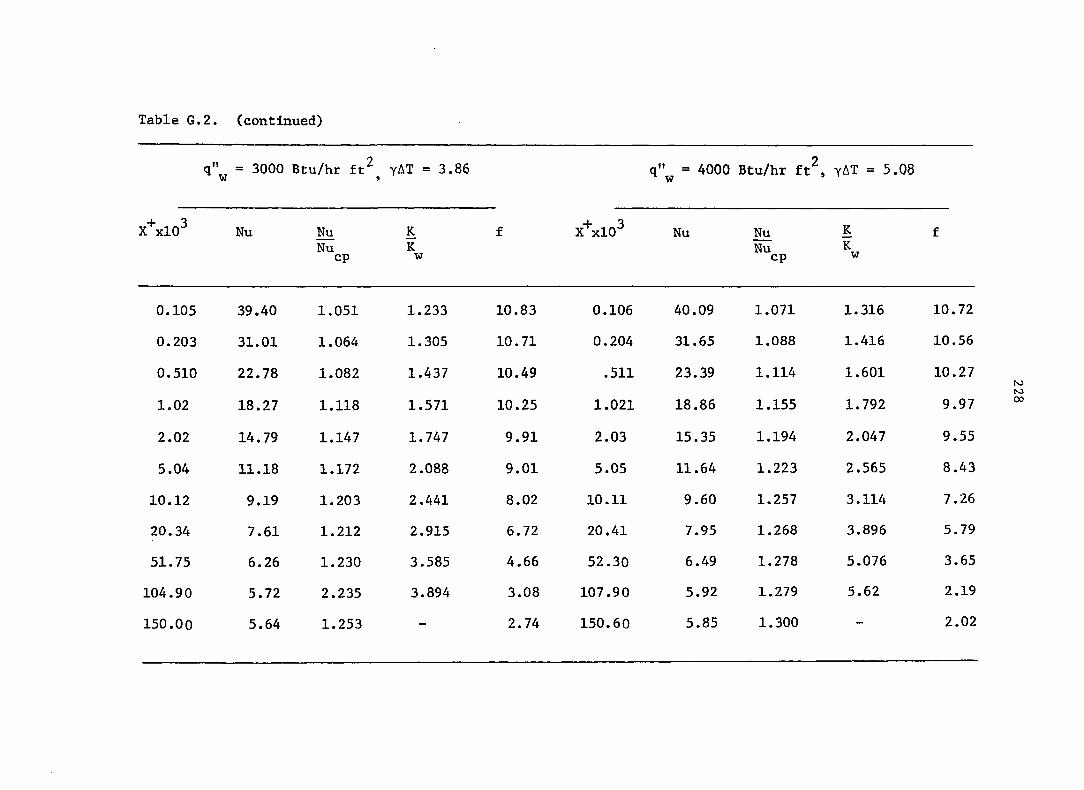
Table G.2. (continued)
q"^ = 3000 Btu/hr ft^^ yAT = 3.86 q"^ = 4000 Btu/hr ft^, yAT = 5.08
+ 3 X xlO Nu Nu
Nu cp
K K w
f + 3 X xlO Nu Nu
Nu cp
K K w
f
0.105 39.40 1.051 1.233 10.83 0.106 40.09 1.071 1.316 10.72
0.203 31.01 1.064 1.305 10.71 0.204 31.65 1.088 1.416 10.56
0.510 22.78 1.082 1.437 10.49 .511 23.39 1.114 1.601 10.27
1.02 18.27 1.118 1.571 10.25 1.021 18.86 1.155 1.792 9.97
2.02 14.79 1.147 1.747 9.91 2.03 15.35 1.194 2.047 9.55
5.04 11.18 1.172 2.088 9.01 5.05 11.64 1.223 2.565 8.43
10.12 9.19 1.203 2.441 8.02 10.11 9.60 1.257 3.114 7.26
20.34 7.61 1.212 2.915 6.72 20.41 7.95 1.268 3.896 5.79
51.75 6.26 1.230 3.585 4.66 52.30 6.49 1.278 5.076 3.65
104.90 5.72 2.235 3.894 3.08 107.90 5.92 1.279 5.62 2.19
150.00 5.64 1.253 — 2.74 150.60 5.85 1.300 - 2.02

Table G.3. Flow behavior index, n = 0.5
q" = 1000 Btu/hr ft^, yAT =1.34 w
+ 3 S xlO Nu Nu
Nu cp
K f
0.156 24.57 1.017 1.083 3.69
0.303 27.15 1.036 1.107 3.67
0.511 22.66 1.039 1.129 3.65
1.02 17.98 1.051 1.165 3.62
2.02 14.40 1.066 1.211 3.58
5.03 10.83 1.087 1.289 3.51
10.08 8.81 1.100 1.366 3.35
20,15 7.27 1.108 1.458 3.14
50.77 5.95 1.112 1.58 2.74
102.60 5.48 1.123 1.63 2.31
150,00 5.36 1.123 2.24
q"^ = 2000 Btu/hr ft^, yAT =2.62
H- 3 S xlO Nu Nu K f
Nu K cp w
0.156 35.56 1.029 1.168 3.61
0.307 27.98 1.068 1.218 3.58
0.518 23.48 1.092 1.264 3.55
1.03 18.79 1.105 1.340 3.50
2.03 15.28 1.140 1.433 3.45
5.05 11.51 1.160 1.612 3.24
10.09 9.44 1.180 1.787 3.00
20.28 7.82 1.194 2.009 2.65
50.90 6.42 1.202 2.312 2.05
104.39 5.87 1.209 2.458 1.50
150.00 5.77 1.210 — 1.33

Table G.3. (continued)
q"^ = 3000 Btu/hr ft^. YAT = 3.87 q"^ = 4000 Btu/hr ft^. YAT = 5.12
+ 3 X xlO Nu Nu
Nu cp
K Kw
f + 3 X xlO Nu Nu
Nu cp
K Kw
f
0.156 36.47 1.073 1.254 3.54 0.159 37.35 1.105 1.343 3.47
0.309 28.86 1.106 1.331 3.50 0.311 20.71 1.143 1.449 3.42
1.00 19.80 1.151 1.517 3.39 1.00 20.62 1.199 1.705 3.28
2.01 16.16 1.193 1.666 3.32 2.03 16.92 1.255 1.915 3.20
5.04 12.16 1.222 1.968 3.02 5,06 12.74 1.287 2.364 2.84
10.11 10.02 1.254 2.267 2.71 10.16 10.50 1.313 2.825 2.47
20.39 8.25 1.262 2.682 2.26 20.49 8.64 1.320 3.496 1.96
51.96 6.72 1.266 3.280 1.57 52.42 6.95 1.320 4.560 1.23
106.70 6.15 1.266 3.545 1.03 102.51 6.41 1.320 4.948 0.77
150.00 6.04 1.266 0.96 150.00 6.30 1.321 — —

231
APPENDIX H: THE PREPARATION OF PSEUDOPLASTIC FLUIDS
In this study, the working fluids were two aqueous solutions;
0.9 percent and 1.0 percent by weight of polymer XD - 7630.02
(hydroxyethylmethy 1 cellulose, HEMC, Dow Chemicals) were prepared in the
laboratory. These aqueous solutions were selected because
1. They are definitely pseudoplastic fluids.
2. They are fairly stable.
3. There is no health or fire hazard associated with their use.
4. They are relatively easy to obtain and prepare in large
quantities.
5. These fluids, with 0.9 percent and 1.0 percent concentration,
are quite viscous (100-200 cps), yet they could still be
handled by the gear pump installed in the test loop.
In the following section, a method is described to prepare the
0.9 percent HEMC solution [104].
Method of Preparation
In a large glass tank 80 lbs (about 10 U.S. gallons) of distilled
water was precisely measured. In this water at room temperature,
0.72 lbs of polymer powder was gradually added. During addition, the
water was mildly agitated with the help of an aluminum rod to disperse
the powder uniformly throughout the entire solution and to avoid any
globule formation. This surface treated powder readily dispersed in
the water and gave a milky white solution.

232
This solution had a pH value of about 5.0, which was estimated by
using pH paper. A one molar solution of NaOH was added (in drops) to
this polymer solution to raise its pH value. The polymer solution was
agitated while the alkaline solution was added as to bring about a uniform
dispersion. As the pH value of the solution started rising, the
solution became more and more viscous, .and at about 8.5 pH a crystal-
clear, highly viscous solution was obtained.
A similar procedure was followed to prepare the 1.0 percent
solution. It is important to emphasize here that these two solutions
are quite close in their concentration. However, these two solutions
have a distinctly different flow curve and they exhibit different
ranges of K and n.

233
APPENDIX I; FLUID FLOW CURVES
The fluid flow curve is a plot of shear stress, T, against shear
rate, du/dy. The constitutive equation of the pseudoplastic fluid is
T = K(du/dy)" (1.2)
This equation can be rewritten as
log T = log K + n log (du/dy) (I.l)
This is a log-linear equation with consistency index K as the intercept
on the T axis at unit value of du/dy, and n is the slope of this straight
line.
For the pseudoplastic fluids, the constitutive equation is also
written as [1]
T = K* (8Û/D)" (1.2)
8u/D is the slope of the velocity profile at the wall for Newtonian
fluids. Furthermore
K' = K (^^)" (1.3) 4n
The log-linear Eq. (1.2) was used to obtain the fluid flow curve. The
actual test section with those pressure taps was effectively utilized
to estimate this fluid flow curve. For in-tube hydrodynamically
developed flow

234
and (8u/D) was evaluated from the known fluid flow rate and tube geometry.
This simple straight tube viscometer was used by Oliver [68], and Scheve
[105] demonstrated the effectiveness of such a viscometer (rheometer)
for non-Newtonian fluids.
Experimental Procedure
The experimental setup here is essentially the same as that described
in Chapter VI and shown in Fig. 6.1. The test section I (Fig. 6.3) was
used as a tube "viscometer." This test section has a hydrodynamic entrance
length, AB (3.5 ft) and a measuring length BC (5.98 ft) across which the
pressure drop was measured by a mercury manometer.
The fluid was circulated through the test loop with a gear pump.
The fluid flow rate through the test section was precisely adjusted by a
needle valve placed upstream of the hydrodynamic entrance length, AB.
The inlet temperature of the fluid was adjusted by monitoring heat input
in the top surge tank and preheater and the cooling in the heat exchanger.
The test section was heavily insulated, and hence, within about 15 minutes,
all thermocouples on the test section and fluid inlet and outlet thermo
couples read within 0.5°F, and, thus, throughout the test section an
isothermal condition was established. Normally it took about half an hour
to establish steady thermal and hydrodynamic conditions. Once this
steady-state was reached,
1) Pressure drop was recorded from the mercury manometer and
was estimated from Eq. (1.4).
2. Fluid flow rate was measured by a weigh tank, and (8u/D) was
calculated.

235
These data were obtained for various flow rates at t = 65.0, 100,0, 115.0,
and 130.0°F. The data are presented in Figs. I.l and 1.3.
Fluid Degradation
The pseudoplastic fluids are basically polyaer solutions. Due to the
circulation through the test loop via the gear pump as well as various
heating and cooling processes in the test loop, the fluid polymer chains
tend to break down with time. This fluid degradation with time, which is
also known as aging, caused a noticeable change in values of K and n with
time. In general, K decreased while n increased with time. As mentioned
in Chapter VI, to account for this aging, the following procedure was
developed.
For solution I (0.9 percent HEMC), 19 heat transfer runs were made.
The K and n values for each temperature were estimated at
Time I: before the start of heat transfer experiments
Time II: after 10 heat transfer runs (about 48 hours)
Time III: after 19 heat transfer runs (about 75 hours).
As shown in Fig. I.l, a significant effect of degradation was
observed. To all these data linear regression correlations (95 percent
confidence) were fit as
= K' (Su/D)"^ (1.2)
These correlations are tabulated in Table I.l. The correlation coefficients
of these correlations are of the order of 0.99, exhibiting an excellent
pseudoplastic (log-linear) relationship.
The arithmetic averages of correlations for Times I and II were used
to reduce data for Runs 1 to 10 and similar averages of correlations for

SOLUTION I: 0.9% HEMC SOLUTION
O TIME I A TIME II • TIME III
% 100°F
130
TIME DEGRADATION
Oi.1 100 1000
(8Û/D)(sec~^)
Fig. I.l Flow curve for 0.9% HEMG solution.

Table I.l. Correlations for Solution I (0.9 percent HEMC)
Situation
runs)
65°F 100°F 115°F 130°F
K'xlO^ n K'xlO^ n K'xlO^ n K'xlO^ n
Time I (before the 2.7086 0.54 0.8602 0.65 — — — — start of heat transfer runs)
Time II (after 1.9350 0.59 0.8009 0.65 0.40369 0.70 0.2440 0.76 10 heat transfer runs)
Time III (after 1.8610 0.58 0.5582 0.69 0.344 0.73 0.1644 0.80 19 heat transfer
Correlation: = K' (8u/D)^; the correlation coefficients were of
the order of 0.99 in all of the above correlations.

238
Times II and III were taken to reduce data for runs 10 to 19. These arith
metic averages are plotted in Fig. 1.2. and tabulated in Table 1.2.
A similar procedure was followed for Solution II (1.0 percent HEMC
solution) . For this solution 9 heat transfer runs were made and, hence,
K and n data were obtained at
Time I: before start of heat transfer runs
Time II: after 9 heat transfer runs (about 48 hours).
Data for Times I and II are plotted in Fig. 1.3 and correlations from
these data are tabulated in Table 1.3. The average results for Times I
and II are plotted in Fig. 1.4 and are tabulated in Table 1.4.
The details of these data and calculations are documented in ISU
Heat Transfer Laboratory files.
Philosophy of time averaging
As noted in the preceding discussion, the K and n results at various
times were correlated, and averages of the correlations were taken to
account for the degradation with time. These K and n plots were used to
calculate various viscosities such as apparent viscosity and effective
viscosity,
^eff = V(8u/D) (3.28)
= K' (8u/D)"/(8u/D)
= K' (8u/D) n-1 (I.11)
and (1.3)

239
4x10 AVERAGE OF TIME I AND II
K (CALCULATED, EQ. (1.3))
AVERAGE OF TIME II AND III
—K (CALCULATED, EQ.(1.3))
1x10
AVERAGE TIME I AND II
AVERAGE TIME II AND III
1x10 150 180 100
Fig. 1.2 Average values for Solution I (0.9% HEMC).
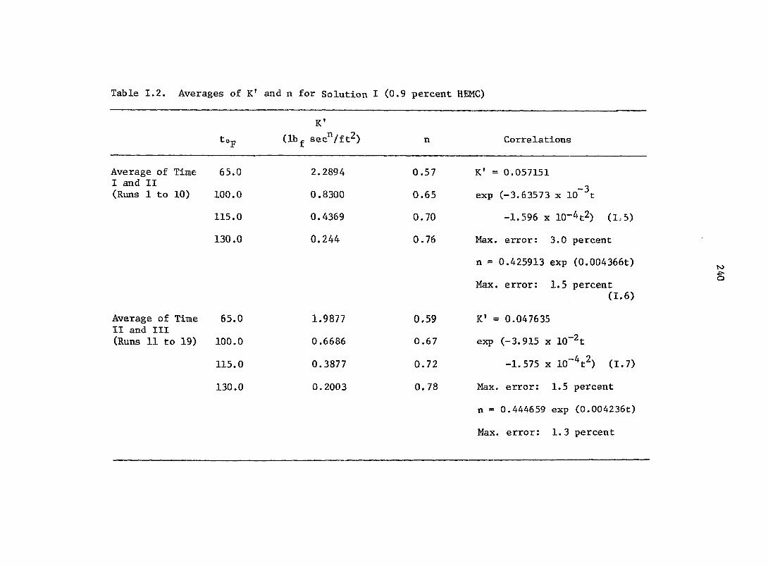
Table 1.2. Averages of K' and n for Solution I (0.9 percent HEMC)
K'
(lbjg sec"/ft^) n Correlations
Average of Time I and II (Runs 1 to 10)
Average of Time II and III (Runs 11 to 19)
65.0
100.0
115.0
130.0
65.0
100.0
115.0
130.0
2.2894
0.8300
0.4369
0.244
1.9877
0.6686
0.3877
0.2003
0.57
0.65
0.70
0.76
0.59
0.67
0.72
0.78
K' = 0.057151
-3 exp (-3.63573 x 10 t
-1.596 X 10⁻⁴t2) (1,5)
Max. error: 3.0 percent
n = 0.425913 exp (0.004366t)
Max. error; 1.5 percent (1.6)
K' = 0.047635
exp (-3.915 X 10~^t
-1.575 X lO'^fZ) (1.7)
Max. error: 1.5 percent
n = 0.444659 exp (0.004236t)
Max. error: 1.3 percent

T 1 1 1—r
h SOLUTION II: 1.0% HEMC SOLUTION A TIME I
O TIME II
r—r—r
65° F
130° F
J L 40
J 1—I—L
100 J I I I I L
(8Û/D) {sec~b
1000
Fig. 1.3 Flow curve for 1.0% HEMC solution.
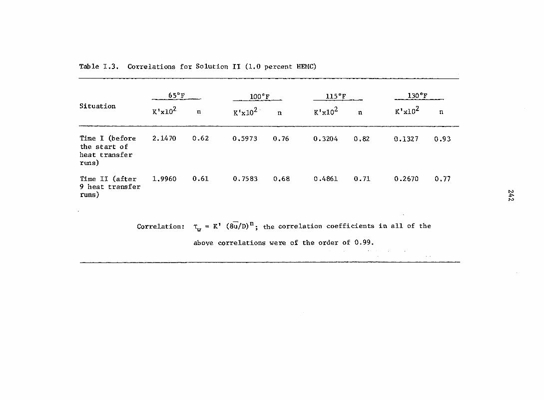
Table 1.3. Correlations for Solution II (1.0 percent HEMC)
65°F 100°F 115°F 130°F
Situation o „ o ? K'xlO^ n K'xlO n K'xlO^ n K'xlO n
Time I (before 2.1470 0.62 0.5973 0.76 0.3204 0.82 0.1327 0.93 the start of heat transfer runs)
Time II (after 1.9960 0.61 0.7583 0.68 0.4861 0.71 0.2670 0.77 9 heat transfer runs)
Correlation: = K' (8u/D)^; the correlation coefficients in all of the
above correlations were of the order of 0.99.

243
0.03 1 1 1 r
0.01 -
CM
O (U (/>
4-
o
<
] 1 1 r
AVERAGE OF TIME I AND II
O K'
A n
——K (CALCULATED, EQ.(1.3))
1.0
0.0011 1 1 1 1 1— L I I L_ 50 100
t (°F)
Fig. 1.4 Average values for Solution II (1.0% HEMC)
0.1 150

Talbe 1.4. Averages of K* and n for Solution II (1.0 percent HEMC)
t °F
k ' Ibf sec^/ft^
Average of time I and II
65.0
100.0
115.0
130.0
2.0701
0.6729
0.3559
0.1908
n Correlations
0 . 6 2
0.72
0.78
0.85
K' = 0.070103
exp (-0.966 X lO"^^.
-1.3951 X 10⁻⁴t2) (1.9)
Max. error: 2.0 percent
n = 0.450709
exp (0.004805t)
Max. error: 1.2 percent (I.10)

245
For the given fluid, is dependent on temperature, (8u/D), and
time (or, more strictly speaking, time and flow conditions) . In order to
evaluate the relative effect of time and temperature variation on
yg££, for a given and temperature, the change in with time was
evaluated. This is plotted in Fig. 1.5, for solution II at = 0.4 and
0.25 Ibf secP/ft2. Similarly, at these shear stress values, at a given
time level, the change in due to temperature was evaluated. This is
also plotted in Fig. 1.5. This figure distinctly demonstrates the
dominance of the temperature effect over the time effect. The change
in y^ff due to time effects was linear and, hence, the time averages
were taken to account for these effects.

100
I
4-
3
.•« 60 4-
II
<J
O CONSTANT TEMPERATURE, VARIABLE TIME (ABOUT 48 HOURS) ^ CONSTANT TIME, VARIABLE TEMPERATURE
\ = 0.25
\ = 0.40
= 0.25
= 0.40
lU 20 30 40 50 60 70
At = (t - 65)0 p
Fig" 1*5 Plot of percentage change in effective viscosity against temperature difference.
N5
ON
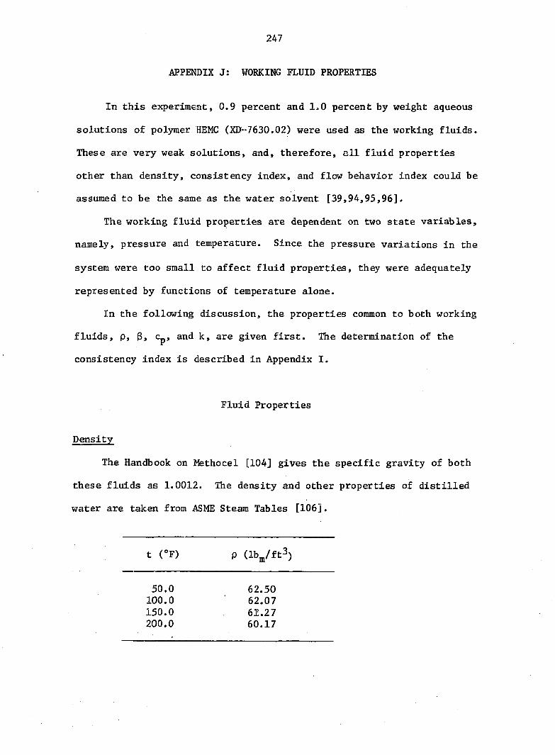
247
APPENDIX J: WORKING FLUID PROPERTIES
In this experiment, 0.9 percent and 1.0 percent by weight aqueous
solutions of polymer HEMC (XD-7630.02) were used as the working fluids.
These are very weak solutions, and, therefore, all fluid properties
other than density, consistency index, and flow behavior index could be
The working fluid properties are dependent on two state variables,
namely, pressure and temperature. Since the pressure variations in the
system were too small to affect fluid properties, they were adequately
represented by functions of temperature alone.
In the following discussion, the properties common to both working
fluids, p, 3J Cp, and k, are given first. The determination of the
consistency index is described in Appendix I.
The Handbook on Methocel [104] gives the specific gravity of both
these fluids as 1.0012. The density and other properties of distilled
water are taken from ASME Steam Tables [106].
assumed to be the same as the water solvent [39,94,95,96]
Fluid Properties
Density
50.0 100.0 150.0 200.0
62.50 62.07 61.27 60.17

248
The equation for these data are
p = 1.0012 (62.422 - 0.21862% - 0.21785n2
+ 0.001077 n^) lbm/ft3 (J.l)
where
n = t - 50°F 50°F
Temperature range; 50-200°F
Maximum error: 0.02 percent
Isobaric thermal expansion coefficient
The isobaric thermal expansion coefficient is defined by the
equation
3 = - (|^) (J.2)
using Eq. (J.l), g is written as
o ^ -0.21862 - 0.43570n + 0.03231 . 1_ ^ 50(62.422 - 0.21862n - 0.21785 + 0.01077 n-^ °F
(J. 3)
where
n = t - 50.0°F 50.0°F

249
Isobaric specific heat
The variation in Cp with temperature is very small andj therefore,
Cp was assumed to be constant:
Cp = 1.0 Btu/lb^/'F (J.4)
Temperature range; 50-180°F
Maximum error; 0.2 percent
Thermal conductivity
The data points are
t k °F (Btu/hr ft °F)
50 0.3392 100 0.3633 150 0.3806
They are described by the following equation
k = 0.3392 + 0.0275n - 0.0034 ^ (J.5) nr rt F
where
t - 50.0°F n = 50.0°F
Temperature range; 50-200°F
Maximum error; 0.13 percent

250
Consistency Index and Flow Behavior Index
The graphical data given in Appendix I are described by the
following equations:
Solution I (0.9 percent HEMC, Runs 1 to 10)
K' = 0.057151 exp (-3.63573 x 10~^t - 1.596 x 10-^;:2) (1.5)
Maximum error: 3.0 percent
n = 0.425913 exp (0.004366t) (1.6)
Maximum error: 1.5 percent
The correlation for calculated K, Eq. (1.3), is similar to that for K',
Eq. (1.5); however, a log-linear expression was fitted to small portions
of the K-t curve (Fig. 1.3).
for 55 to 65°F
K = 0.088962 exp (-0.022326t)
for 65 to 75°F
K = 0.109202 exp (-0.025479t)
for 75 to 85°F
K = 0.138329 exp (-0.028632t)
for 85 to 95°F
K = 0.180966 exp (-0.031793t)
for 95 to 105°F
K = 0.244018 exp (0.034939t)
for 105 to 120°F
K = 0.369801 exp (-0.038874t)
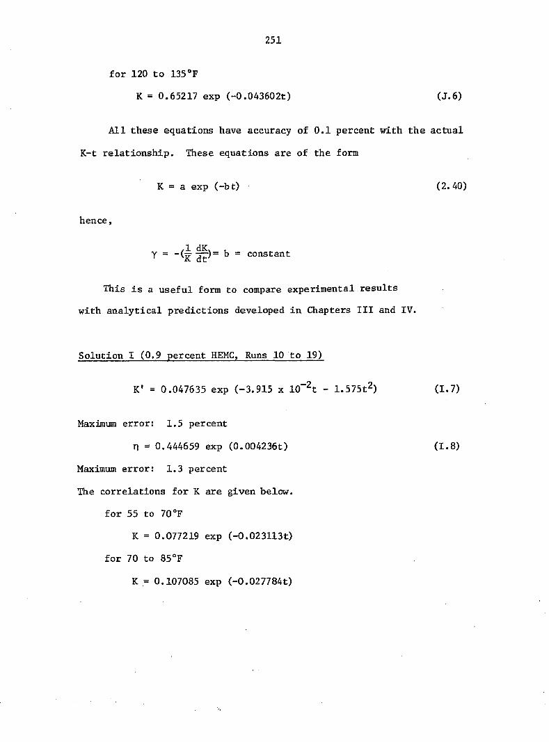
251
for 120 to 135°F
K = 0.65217 exp (-0.043602t) (J.6)
All these equations have accuracy of 0.1 percent with the actual
K-t relationship. These equations are of the form
K = a exp (-bt) (2.40)
hence,
Y = h = constant
This is a useful form to compare experimental results
with analytical predictions developed in Chapters III and IV.
Solution I (0.9 percent HEMC, Runs 10 to 19)
K' = 0.047635 exp (-3.915 x lOT^t - 1.575t2) (1.7)
Maximum error: 1.5 percent
n = 0.444659 exp (0.004236t) (1.8)
Maximum error: 1.3 percent
The correlations for K are given below.
for 55 to 70°F
K = 0.077219 exp (-0.023113t)
for 70 to 85°F
K = 0.107085 exp (-0.027784t)

252
for 85 to 95°F
K = 0.148708 exp (-0.031678t)
for 95 to 110°F
K = 0.215591 exp (-0.03556t)
for 110 to 120°F
K = 0.33017862 exp (-0.039459t)
for 120 to 135°F
K = 0.52674 exp(-0.043329t)
for 135 to 150°F
K = 0.989871 exp (-0.048001t) (J.7)
All these equations have accuracy of 0.1 percent with the actual K-t
relation.
Solution II (1.0 percent HEMC, Runs 1 to 9)
K' = 0.0701034 exp (-0.6604 x lO'^t - 1.395 x lO'^tZ)
(1.9)
n = 0.450709 exp (0.004805t)
The correlations for K are given below.
for 55 to 70 °F
K = 0.105895 exp (-0.0265t)
for 70 to 95°F
K = 0.188437 exp (-0.03403t)
for 95 to 110°F
K = 0.261398 exp (-0.03745t)

253
for 110 to 130°F
K - 0.444107 exp (-0.0422419t) (J.8)
All thèse equations have accuracy of 0.1 percent with the actual K-t
relationship.

254
APPENDIX K: SAMPLE CALCULATIONS
Run No. 13 for solution I (0.9 percent H EMC) is used here to
illustrate the data reduction procedure. In the following discussion,
all fluid properties were evaluated at bulk temperature unless mentioned
otherwise.
Physical dimensions and properties of the tube
Inside tube diameter, D = 0.401 in.
Outside tube diameter, D1 = 0.441 in.
Total heated length, L = 71.8 in.
Length up to measuring station No. 4, Lg = 60.4 in.
Thermal conductivity of the tube, kl = 9.4 Btu/hr ft °F
Length between the pressure taps = 73.9 in.
Measured quantities
The tube wall thermocouples readings at the measuring station were
numbered 1 to 3. These thermocouples were 120° apart. The two thermo
couples placed in the flow at the inlet and outlet section were
Numbers 13 and 14.
The measured data were as follows:
Experimental Parameters
t^ = 146.76°F
t^ = 147.01°F
t^ = 146.52°F
t^^ = 98.10°F
t^3 = 65.57°F

255
Fluid flow rate (measured by weigh tank) = 78.10 Ib^^/hr
Voltage across the test section, = 7.98 volts
Voltage across the shunt, Vg = 41.007 mv
Pressure drop = 1.25 in. of mercury
Room temperature = 79.0°F
Experimental Calculations
Heat flux calculations
The heat loss through the insulation was estimated to be 1.5 percent
[53,54,83], and, therefore, the net heat supplied to the fluid was
I = 2.4 Vg
= 2.4 X 51.007 = 98.42 amps
The heat loss through the insulation was estimated to be 1.5 percent,
and, therefore, the net heat supplied to the fluid was
Q = 0.985 V^I
= 0.985 X 7.98 x (98.42) x 3.4129
= 2640.14 Btu/hr
The average heat flux, q^, based on the inside tube surface area
was
q" = Q ^ w ïïDL
= 2640.14 X 144 TC X 0.401 X 71.8
= 4205.73 Btu
hr ft^

256
The rate of volumetric heat generation was calculated as
q'' =
4 ("ï - B ) I-
_ 4 X 2640.14 X 144 x 12
Tr[(0.441)2 - (0.401)2] 71. g
= 2.402 X 10^ Btu/hr ft^
The temperature drop across the tube wall was calculated [54,83] as
. I»
t =14 [(Dl)2 In (Dl/D) - I ((01)2 _ 0%)] w 8 kl ^
= [(0.441)2 in (0^^^^
- \ (0.441)2 - (0.401)2]
= 0.37°F
The above temperature drop was applied uniformly around the
circumference of the tube so as to obtain the following inside wall
temperatures :
tj_ = 146.39°F
tg = 146.64°F
t^ = 146.15°F
Simpson's rule was used to compute average wall temperature as
t, = 146.39°F w

257
Fluid bulk temperature
The fluid flow rate was measured by using a weigh tank;
m = 78.18 Ib^/hr
An energy balance over the tube length from the onset of heating up to
measuring station yields
Q — = mcp
0 L hence, t, =• (y—) + t
b mCp L o
= (IH) +
= 93.98°F
Nusselt number
The circumferentially averaged heat transfer coefficient was
calculated as
tw - tb
4205.14 " 146.39 - 93.98
= 80.25 Btu/hr ft^ °F
The above calculated h and the thermal conductivity k of the
solution at bulk temperature were used to calculate the Nusselt number:
Nu = k
^ 80.25 X 0.401 0.361 X 12
= 7.43

258
Effective viscosity
K' and n were evaluated from the respective property correlations.
K was calculated as
K = K' (4n/3n+l)*
At this station
K' = 8.20 X 10"^ and = 9.19 x lO'^ (Ibj sec")/ft2
n = 0.66 and n =0.83 w
K = 7.57 X 10⁻³ and = 8.79 x lO"^ (ib^ sec")/ft2
— = 8.62 Kw
Wgff = K' (8Û/D)*-1
= 32.2 X 8.20 X 10-3 (8 x 0.398 x 12)0-66-1 0.401
= 0.057 lb /ft sec m
similarly, = 0.013 lb /ft sec ^ m
Dimensionless numbers
Reynolds number,
.ûîTn , 62.28 X 0.398 x 0.401 = 12 X 0.057
= 14.6
similarly, (Re) = 61.8

259
Prandtl number.
^ eff^P ^ 0.057 X 1 X 3600 k 12 0.361
= 564.5
similarly, Pr^ = 127.0
Dimensionless distance,
X+ = 2CX/D) 2(60.4/0.401) RePr 14.6 X 564.5
= 3.65 X 10⁻²
similarly, = 3.84 x lO'^
Graetz number^
G: = - 78-18 * 1 k X 0.361 X (60.4 x 12)
= 43.1
Comparison with numerical solution
As mentioned in Appendix J, the present K-t curve was of the type
K = a exp (-bt - ct^)
but a curve of the type
K = a exp (-bt)
was fit to each 15-20°F interval, and from these equations y was evaluated
at fluid bulk temperature (see Appendix J).

260
= 4205.73 X 0.401 (0.0355) 2 X 12 X 0.361
= 6.17
Cg = C^yAT - CgfyAT)?
= (0.12392 - 0.05420n)YAT - (0.010133 - 0.0068n) (yAT)^
with n = 0.66, C = 0.33
(Jiy_) = 1.0 + C. = 1.0 + 0.33 Nu max K Nu^p max
= 1.33
The exponent of the viscosity correction was calculated as
m = 0.58 - 0.44ri
= 0.58 - 0.44 X 0.66
= 0.29
Then (|-) = (1.33)l/°'29 crit
= 2 . 6 8
Hence, (K/K^) >
The consistency correction was thus calculated as follows ;
The exponent of the consistency correction at wall
m = 0.58 - 0.44n w w
= 0.58 - 0.44 X 0.83
= 0 .22

261
The consistency correction is then
= (2.68)°-22
= 1.24
The non-Newtonian correction is
= 1.02
Now, Nusselt number, Nu. = 7.43
The corrected non-Newtonian Nusselt number is
7.43 (â„)l/3 1.02
= 7.31
Finally, the consistency corrected non-Newtonian Nusselt number is
7.31
(Aw)l/3(Cc)M 1-24
= 5.91
This value is at = 3.65 x 10"^; the corresponding numerically
calculated value at this is 6.12, thus, showing 0.35 percent error.

262
Friction factor
The reynolds number at the middle section of the tube is given by
Re = GSH = 11,7
m ueff
and fluid properties were evaluated at
t = am 2
The pressure taps on the metal tube were 73.9 in. apart, 1.05 in. outside
the 71.8 in. heated length at each end. It was therefore necessary to
calculate isothermal pressure drops, which need to be subtracted from
the total pressure drop.
At inlet, t =65.67 o
= 62.41 X 0.401 X 0.396 0.0918 X 12
= 9.0
fo = 64/Re
= 64/9
= 7.11
At exit, tg = 98.10
re^ = (pdu/y^^^)^
= 62.09 X 0.401 X 0.399 0.0519 X 12
= 16.0

263
fg = 64/reg
= 64/16
= 4.0
The isothermal pressure drops across the unheated inlet and outlet
segments were calculated as
fL pu
7.11 X 1.05 X 62.41 X (0.397) x 12 12 X 32.2 X 0.401 x 2
=2.84 Ibf/ft
fL pu ""a =
4 X 1.05 X 62.09 x (0.399)% x 12 12 X 2 X 32.2 X 0.40
= 1.61 ibf/ft^
The total measured pressure drop as calculated from the differential
mercury head, AH, is given by
Apt = AH (Pgg - PHEMC oom temp
= -ijp. (847.37 - 62.32)
= 81.78 lb /ft%
Finally, the pressure drop across the heated section is
apj^ = ap^ - ap^ - ap^

264
= 81.78 - 2.84 - 1.61
= 77.33 Ibg/ftZ
= 0.537 psi
• •
= 2 X 32.2 X 0.401 x 77.33
62.24 X (0.398)2 g
= 2.98
A listing of the FORTRAN IV computer program utilized to facilitate
the data reduction is given in Appendix L. The experimental results for
heat transfer and friction factor are tabulated in Appendix M.

265
APPENDIX L: COMPUTER PROGRAM FOR EXPERIMENTAL DATA REDUCTION

266
C COVPUTJCNAL PHLCECLRE FCJH THE CATA Rf .OUCr iGN FOH A NON-NEt iTUN l AN C FLUID FUCK IN A PLAIN TUBE.
REAL NL8 . NUF* NUC. N . MUEF. MUEB. PUEW, KA* . KAB•K .M«L0 tL I
REAL MLE l .MUEM.MUEC .NUL
C OINEKSICK TEMP ( e ) . ThKSI
C C 01 rs INTEKhAL C IAKETER OF THE TUBE
C C 02 l i ; CUTER DIAMETER CF THE TUBE C C TL IS TUTAL HEATED LENGTH C C TL l . T12. r L3 . am : TL4 DENUTE T^E DISTANCES Uh HEAT TRANSFtH C SECTION FRCf THE ChSET OF HEATING^ C C THLTB CENOTE THE THERMAL CONDUCTIV ITY OF THE TUBE
C c
DATA C I . 02 . TL l . TL2« TL3 . TL4 . ThCTb /0 .04221 .0 .046675 . 0 .4063 1 .0 .9»4e .2 .4688 .3 .S688«9 .64 /
DATA T15 ,TL6 .TL7 .TLU.TL /5 .4792 .6 .9792 .7 .8125 .8 .6432 .8 .9696 /
C C L I AND LO DENOTES LENGTH BETWEEN PRESSURE TAP AND HEATED SECTION AT
C INLET AND CUTLET RESPECTIVELY DATA L I . LC / 0 .10417 .0 .02063 /
C c
DATA P l .OC.PCF /3 .141593 .32 .174 .3 .4129 /
C D12=C1#D1 D13=C12*C1 022=D2*D2 AREA=Pf *012 /4 .0
C C CALCULATION CF TFE ELECTRICAL HEAT INPUT
C 1 REAO(5 .2 .ENO=500 ) NR.NS.FL I .M .VLT .VLS .H2 .ROUMT 2 FCRNAT(2 IS .6F10 .4 )
AMP = 2 .4 4 VLS
RT - VLT /APF WAT = 0 .965 * VLT» AMP C ITCT = WAT • PCF OFLLX = OTCT/ (F I * 01 * TL ) FLC* = M • 60 .C
C VOLUMETRIC FEAT GENERATION IS DENOTED BY UPUV QPUV = 4* QTOT / (P I * <D22-D12 ) * TL ) DTW = CPLW * (022»AL0G(O2 /D l l - (<C22 -012 ) /2 . )> / ( e . 0 *THCTBJ WR1TE(6 .501 ) NR.NS.FLOW.FL I .VLT .VLS .AMP.PT .WAT.QTOT.QFLUX
501 FORMAT ( • 1 • . J6X .«FEAT TRANSFER TO NCN-NEWTCN I AN FLUID IN PLA IN IC IRCULAR TUBE» . / . 220X. ' * * * *$**$*** * * * * * * * * * * * * * *#** * * * * * * * * * * * * * * *»*#***#*** * *#** * * *
410X . *RLN NUMBER: * .15 .50X . 'FLU ID : XD-7630 .02 . 1% SCLN. " . / . £10> .«SECTICN : • • ! £ . • / . tSX . "SYSTEM PARAMETERS: ' . / . 75X . ' * *« *# * *# * *4 * * *# * *» ' . / , 810%. "FLUID FLOW RATE = • .F10 . j . 2X . ' LBM/HR* .30X . •FLCW 1 INCEX= ' . FS .S . / / . 91 OX. 'VOLTAGE ACROSS THE TUBE = ' .F10 .3 .2X . •VOLTS• . • / .

267
910X . •VCLTACE ACHOSE THE SHUNT = • .F10 .3 ,2X . •M ILL1 -VCUTS» . / / . 9 I0X .«C tHNENI THROOtH TH t TUBE = • .FJO.4 .2X , •AMPS• . 910X .«RESISTANCE CF THE TUbE = ' .E1%.6 .2X . 'OHMS ' , / / , 910X . 'ELECTRICAL KE fT INPUT = ' .F10 .3 ,2X , 'WATTS ' . / / , « lOX . 'TCTAL MEAT INPUT = ' .F I0 . J .2X , *8TL /HR« . / / , 9 Î0X . 'TOTAL INPLT HEAT FLUX = ' «F 10 .3«2X , •BTU/<HR-SC.FT I ' )
C C CALCULATION OF WALL TEMPERATURE C
REAC ( 5 ,5 ) (TEMPI 1 ) , 1 = 1 ,51
5 FCKKAT (SF10 .41 DO 10 1=1 ,3
10 TM1( I )= TEMPI I ) - CTW
C C S IMPSCNS RULE IS USEC TO CALCULATE MEAN WALL TEMPERATURE
C Tk *= (T* I (1 )4 -4 . »T * I ( 2 ) + TW1(3 ) ) / 6 ,
C C CALCULATION OF THE FLUID TEMPERATURE
C TEMPIN = TEMPI 4 ) TEMPCU = TE#P ( 5 ) aOLT=FLùk* (TEMPCU-1EMP1N) QDIF r=100 .0 4( 0TUT-COUT) /QTOT TLTC=TL l IF (NS.EC.2 ) TLrC - IL2 IF(hS.E0 .3) TLTC=T13 IF (NS.Ea .4 ) TLTC=TL4 IF INS.EC.S) TLTC=TL5 IF (6S.EC.6 ) TLTC=TL6 IF (NS .EC . 7 ) TLTC=1L7 IF (NS .EC .a) TLTC=TL8 GI»=CTCT$TLTC /TL TF8=(QIN/FLOW)+TEMFIN TFL%=( IFE+TWMl /Z .O
C DELTAT=TkM-TF8 HTC=GFLUX/OELTAT
C NUE=HTC*D1 /THCNL( IFB)
C G Z e =FLC* i / (ThCNL(TFE)»TLTC)
G^h=CZB4THCNL(TFdJ /THCNL(TWM) PLL .sxB=p i / ( 2 .o «cze J PLLSXh=PI / (2 .0 *02* ) WHITE(e ,504 ) TMK I ).TW1 (2 ) , T WI ( 3 ) , TM M. TEMPI N» TEMPOU.TFB . TFLN.Q IN .
IQCt l .OCIFF £04 FCPMAT( ' 0 ' »5X , 'TOBE *ALL TEMPERATURES ' , / ,
15X , ' # * * *# * * * *#4 *$ * *# * * * *# * *# , , / / , 235X .F10 .2 , / / , 4SX .F i0 .2 . / / , 3SX , r i 0 .2 . / / , 31 OX, 'MEAN HALL TEMPERATURE = * ,F10 .2 ,2X , 'F ' . / / ,
410X , ' INLET FLUIC TEMPERATURE - • ,F10 .2 ,2X , 'F ' 510X , 'OLTLGT FLUID TEMPERATURE = ' ,F10 .2 .2X , 'F« , / / , 710X . 'FLU ID BUCK TEMPERATURE = ' ,F10 .2 ,2X , •F ' , / / . 81 OX, 'MEAN FLUIC TEMPERATURE = ' .F10 .2 ,2X , 'F ' 91 OX. 'HEAT INPUT LP IC LENGTH X = ' , F10 .3 ,2X , ' 8TU /MR ' , / / , 91 OX, 'HEAT OUTPUT = • .F10 .3 .2X , 'BTU/HR ' . / / , 91 OX, 'PERCENTAGE MEfT BALANCE = ' ,F10 .3 , / I
WRITE(£ ,510 ) HTC.MU,GZW.GZW,PLLSXB,PLUSXW 510 FCKMATC 0 ' . 5X . ' I rEAT TRANSFER RESULTS ' . / ,

ti) •0 o
A r .
m o n o > • ^ "n ^ ir. tî o h o ^ w x
« 7: \ 7: I X
V r - C m . . m > 0 X ir
z V) 0.' I m 0
I T m X < -4 > > z m T l -4 A c r m "n < r r a
* >
z t X 0 > < m r u i -4 X r L: Xr 9
A Z 0 0 Z c <r c r A z H >
< 0 a r D > 33 T. r rr. > r W %
r r X •H Z
II m a II II X
S z ro fo f m m
< m ( f
U) 0 a - A
> r o f\) t X X
*0 % >
r r g m ( t T> ' n 0 1 X (f tn > m fn m n n * * # «-z z s s <A -Tî C •4
< " % X o »- 25 X 7 c
a h m fi il Z m il 7 * ^ -H 4 r»
•< < > > X X
il m. o
tp X V «-» *
%: r — c « CD S «*> w X # z
r: z c n s <
(/) o u
z X r > A V i l w < m
a *
o x o X w
U) • \ gr r Cl g x >
« c • «
— t3
• s o ^ • w *
o n o*
< <
m isi
n
z \ 0) 7; * > * s o
o t ) r a > "k u (j u m (»l • o fU o
I « #
c o . m •
w > z r w «• • n ^ V H m» Z . - I
îi
s i » i * n
2 g: o -4 ^ f m z
< 7: >
m £ n I I
ï ? il i
I z
« * rv)
» ^ o
w
X > f * * fv>
( J * z
H g Z
A r. % "C
T
W r» z
V
m <
c c vi c >
cl f\3 O
a a a a a a
a ut (*i fO N Ul
f3 0 S 0 0 X X X X
«• •c X m m «> T» m r > < •n c « Z z m « 0 0 A 0 » -4 r -4 * r 0 < «
w < m » Z m r «-c 7 n «-z c m A «-m z r » m fn c
m < Z 0 « 3) *
C CD < m r C c * r w r #
A % « 0 * C/l
* -4 < «•
« > 9 a s r > > r r r X
r r
II II il II
rv: fo h: ro T! •n Tî m 0 0 0 U)
# w w U
s s K fo s s % X
r m 5 M z S \ en
m •n A H 1 (/) \ m N A
it
en <-* X • < # G
« n « < «F
z C m
Ci CD
; m c V) m en s
I S œ œ ft • 5 %) m m • z • c s . • *0
z m
I
h) •n f z 0 D V Z z z Z 0 A < < n
01 w ro m a 0 n 31 > Z Z 7] m m r c 11 > c > 0 0 0 0 X X X % « CD z T m m 0 r* II II r X X z H II II 11 II f £E r a n C -n A > m c\ w A (M II il il II c m r- C Ci M A IVJ T3 (y Ti Z A A r # n r A z z « Ti 5 0 f 0 r A r\ > T» y > Z) r m > > • ro H 0 c C • « -4 Z s -4 > (A > î < w * 01 •n .• S 7 ; 7v 0 X •4 m H « 7\ m Z * H M n u 0 \ m m « m 0 en r m n W ys -1 H z H a Z 0 Ni r H * T) H « T2 Z w A* T i T l 0
Ni M X # 0
0 > Z Z C 0 0 0 c s Z > # Z 0 c -! « « •n Tî a C z z # Z z -4 m 2 0 n * S 0 m z c m
z C r # F & < Z «• •4 0 m z 4 «
z z Z •ft * « T X Z S m m m « c CE T U » < < CD ne o> n T m T) z fn T) % t » * * f m • r\ m TI Ti CD 73 c 0 c N \ < < n •4 -h CD A « pi M 0 m Z Z H 0 U) c -4 r C C 0 « Z m 07 C C S S z T? c r c m « 1
z N N m m 0 0 H CD * r m • S 1 H H m a < 0 X T » > r H Z î « * «• es fE * r r -n n A « • > < C > A r Œ Z Z 71 m r r z
r r z Z m r X r c m V « > 0 cc z 0 H M '4 - 4 A m cc
-1 m T t TI W >
w z Œ Z 0 -4 r • Y
< r II II z M. II ji 11 II
z 0 0 0
m m m •n T î T) H cr. en
o c' %" s
c z
* « r o
o
z c m s « * r u
o
N) a\ 00
(T o o o • • • • w w w
u
oj M C
I 73
(A O
4i

fi n n r o o
r» n rv
z z z t - r r m m m a % ». Il I I I I C l o Cl
3 2 3 % % x
m m m : : z T) w «o O * M c •» 2 • 09 «
a < Z v o
0) z CD
< " "
S o
* z * * «* * «* "4 »« 2 m Z m z M
o • o o
n Z Z < < < Z) z X M H A > m O z T T X M •N > R IL II II 11 II n O C * M r A z z < < < * M II n R r CD m a H I I II I I C r H M » # » T » X H H r > m 31 X 71 T I I •N M > H tt Z I X I O C c CD z H
n T) O o n A *0 o M M * A Z Z H H •H re T» M M z Z
•N t l •n z m z m • O CD M M
2 V z O
TÎ \ N N z
T3 o M
"N
S S & 2 A M < % X Z M 3} m A n A V S in M * "N A R -T 0 Ô O (A M Q
Z H
"N > n
o
o u o
(f y o
n n a
O OT 4> RU W RU
O 1% X c M "TÏ % N A Z 33 O O O N O X R» 33 *N
*N T l X X V X X M Z M ? H «F
n > m m % •4 z Z z N % M i r m R A > «A, 4% R%
A A TN 3} ΠX O RU CH N I I Cil Z N O a i m m O Z m X 01 0
O < C R > O A
0) Cu m H Z C U1 •H 0) 0) N. O X "H z A z 0) < X #W 2 O N X \K Ci O M C\ n
o Z A R o m A % l«J (/> O F z TL T 2)
T l T î T î N CI X R « Œ < X >
? > M T. Z X ru O» X A U) A X O H \ A 3 ) (/) A Z
RO (N W A 3J z •I Z <
RU < > H l ! M A» II Z f X
X C X z IN X 1 Z c $ (A Z A I R O z •n A V
< < C •D T •fi > H O X TN X M
Z A W (A
*0 ir. z
C o
3
H H Z i l I I I I I I t l C Z CD c
•n -n •n n tl z X m z o o o o o X c • • r u Ul u u » A
> X K V M 0) r Z X X z > < m m 7
> *D o o r r ' • • < c w » CA (A X V V </) CD • •
? c 0) x s
X 2 • C X r *
X Z z <
X X n 7 x m» r A < r a im 11 m (A z M a r a X O X z * 7 r o i mp j X C
A * S Xi ^ X «"h w t %» \ w u
X • z w Z
if z
s
(/) A
s * « X
x x « z il m 0 w • n TN # OC UT 1 0) o I # o ^ # » * X « z x « 7 œ
A A RU #» y 7 I l i l > % fo «—
i m r n w X * * • xx m z z C, CE
* o N fo
w a > * ro fv) U 11 IL ( 0 o o % # > o o _ m »# ## #u
-4 o o A Iw *ti rt) m m a Ui o r\i w Li
CD > M #w il II O o
o •» w
A z z R C PN X A m o s % o o o O o O o O o Tï X X V X V X W X X
Z) X z < X < > > > T l
IÛ V R* 1 1 n TJ X r A o ( r > > (T "D X X o Z (A X X A # > m r
m O X X r (A (A (A A m > a
m M 3) z z m M Z Q -4 > H -H X Z Z > Z < >
r X I X < < D z > Z 31 O X » M r > > •n > (A A m m X •4 z A r FN TL z % z o N TL M Ci R Q C H m z > z r M z "K z a FI •H Z
> (A A % RR c Z X > X Z m C > Z a C > X Z r "0 (A c > Z «H M X r M CD ; 3} z m T M -I ;
C Vi R "4 X I R A > M C s T M X > z z -< X M > r (A H ff
> m •H %
> c >
X A r > H r r m A R r I r r (T X r m C r *
* I I I I I I I I O I I > H I I t r
r •n T î M •n f r II - n fV m M I I m o O O en o # o T Ul u u 0 . 75 o
w O a N s . O s fu N N N N W X N
S C # S N
V S r N o fi
N
m 4
c m A
V
n) on vo

270
KEM=KM(M#C1*VM/MLE* RE I=RHCI#01#V I /MLE I ReC= f iHCe«DI»VO/MLEC
c FRIN I= (4 .0 /KE I FR INC = C4 ,0 /PE0 FR INM=<4 .0 /REM
C •P I=FR1N1«L I *RH014V l«V I / (2aa .O*GC*01 } DFC=FRIN0*L0*HhOE#V0*VO/ (288 .0 *GC*D l ) RHC*T=KHC(mCOMT) rhcwt=fhcme(rccpt) 0PhL=H2#(RHCMT-HHCXT) /1 72 8 .0 0 OFk=CPhL-OF I -DPO FRN=28e .C*GC*D1*CFM/ (RHGM*TL*VM$VM) FRMF=FRM/4 .0 WRITE(e<S60 ) FRM.FPMF.REM
560 FORMAT*»0 " tSX . •FR ICT ION FACraH CALCUTION* . / . ISX.«*$#*#**«#*4###(**$****#*******#*'./. 2 I0X .«FRICr iCN FACICB. OARCYS = ' ,E15 .6 . / , J1OX.«FRICr iCN FACTOR. FANNINGS = ' .E15 .6 . / , 410X . 'VEAN REYNOLDS NUMBERS = ' ,F10 .3 j
C C CALCULATION UF RAVLEIGH NUM8EN
C FH IRT=HkM/FRIhN GAQ=GC#dETA(T8M) *RhCM#RH0M*013*D l *aFLUX/ (MLEM*MUEM*TMCNL(reM)) PHB*=3eOO.O»MUEM*CF(TBM) /THCNL<T8Mi raciw = gfq#prem WR ITE (e .580 ) TFBC. IBM.GUU.PRBM.RAQM.FRIKT
580 FOKMATI 'O" .SX . 'TEMPERATURE OUTLET .MEAN = • .F10 . 2 •«F • .F IO
I . e . 2X ,«F» . / .
25X . •GRASHCF NO. HE4T FLUX BASIS •= • .E1S .6 . / .
35X . "PRANOTL NO. EASED ON MEAN TEMP. = • .F10 .3 , / .
45X . •RAVLEIGH NLW8EP = ' .E15 .6 . / .
S5X , •FR ICT ICh FACTOR (NON- I SO/ ISOTH i = • .F10 .4 )
GC TO I £00 STCF
EhO FUNCTICN RHC(T )
C DENSITY AS A FUNCTIUN OF TEMPERATURE <F» FOR XC-0 .9XS0LN. C LN ITS LBM/CJ jFT
C JATA X1 .X2 .X3 .X4 /62 .422 . -0 .21862 . -0 .21785 .0 .01077 / ETA-<T -60 .0 ) /S0 .0 RHC=(X I+X2*ETA+X3*ETA*ETA+X4* (ETA* *3 .0 ) ) *1 .0012 hetur^ END FUNCTICN BETA (T i
C COEFF IC IENT OF THERMAL EXPANSION AS A FUNCTION OF C TEMPERATURE IF ) FOR 0 .9%S0LUTI0N OF X0^7630 : . 02 C LN ITS 1 /F c
DATA X I .X2 .XJ .X4 / -O .21862 . -0 .4 j 570 ,0e032a%,64=422 /
DATA X£ ,X6 / -0 .217€£ .0 .01077 / ETA-(r-50,0}y50.0 VCL=X1+X2*ETA+X3* (ETA* *2 .0 ) DVCL=X4+X1#ETA+XS*ETA*ETA+X6* (ETA* *3 .0 ) BETA=- (VCL / (SO.O*CVOL>) RETLKN

271
c c <-c
c c c
c c
c c c
c c
XD
UF TEMPERATURE (F )
i£NU FUNCTION ThCNLd i
THEhMAL CCNOUCTIV ITY AS A FONCTION OF TEMPERATURE CF) FCA X0 :0 .9% 76 30 :0 .02
OMIS 8TU/<HH.FT .F )
DATA %1 .X2 .X3 /0 .3JS2 .0 .0275 , -0 .0034 / ET*= (1 -5C .C l /SC .C THChL=* i *X2*ETA+X3*ETA*ETA
RETURN ENC
FOhCI ICN CP< I» SPECIF IC HEAT AS A FUNCTICN
xc-7e3o:0.0£ UMTS eTU/ l LBK .F )
CP=X.C
retlhn EhC REAL FUNCTICN N(1>
N t î h E FLUW BEHfV IOUM INDEX FGR FLU IU X0 :7630.02 N IS CIMENSICNLESS
CA3A XI ,X2 /45.û7Ce73E-02t4B.054E-04/ N=»1*E%P(X2*T» return
END REAL FUNCTICN K ÎT )
K -DASH A£ A FUNCTION UF TEMPERATURE FOR : 0 .9»—7c30 :0 .02
UNITS LdF .SEC**N / (FT*FT) GATA *1,X2 ,X3 /70 .10345E-03. - 96 .6042E-04.-13.95e-05/ K=X1#EXP(X2*T+X2#T*T )
RETLKh end
FOR
DENSITY AS A FUNCTICN OF TEMPERATUkE(F ) , FOR MERCURY FLNCTICN RHONE(T )
UNITS L8M/QU.FT THE TA-<T -68 .01 /E4 .C RHCPE=E47 .7 I - ( 4 .57 *THETA)
RETURN END
FUNCTION EKAd) TH IS FUNCTICN INCICATES CONSTANT IN THE V ISCOSITY POWER INDEX
eKA= .4224 19E-0 i EKA= .374S45E-01 EKA= .340334E-01 eKA= ,306167E-01 EKA= .02650
IF(T .L t .130.0 > I F (T .LE .110 .0 ) IF (T .LE .95 -00 ) IF CTcLL.eS.OO) I F (T .LE .70 .00 )
BKA = - f c KA RETURN ENC FUNCTICN XKA(T )
TH IS FUNCTION INDICATES CONSISTENCY DATA X1 ,X2 / . 1058S5 , -0 .2650E-01 / DATA XJ .X4 /C ,14 1262 . -0 .3061672 -01 /
DATA >5 .X6 /0 .168437* -0 .340334E-01 / DATA >7 .Xa /0 .2613«e . -0 .374545E-01 / DATA >9 .X10 /0 .444107 . -0 .422419E-01 /
INDEX FOR THE FLU ID
i r (T .CT .55 .0 ) XKA=X1*EXP(X2*T )

272
I F (T .GT . rO .O) XK*=XJ*EXP(X4#T1 I F (T .CT .aS .O) XKA=XS*EXP(X6*T ) I F ( r . G T . 9 5 . 0 0 ) X K A - X 7 * E X P ( X 8 « T I I F (T .CT . l 1C .0 )XKA=X9*EXP<XI0 *T )
petukh end

273
APPENDIX M: TABULATION OF EXPERIMENTAL DATA

274
Experimental Results for Solution I (0.9 porrunL HRMC)
Table M.l. Experimental variables
Run m q"w , No. lb /hr Btu/hrft Re Pr f m .
1 to 4 82.02 1104.8 8.5 1061.0 6.46
5 to 8 156.00 1709.2 20.6 837.6 2.72
9 to 12 234.00 2140.1 36.9 702.8 1.54
13 to 16 52.2 1753.0 4.3 1343.7 10.17
17 to 20 52.8 2425.4 4.5 1281.6 8.63
21 to 24 78.6 3246.9 8.0 1080.4 4.90
25 to 28 125.2 2479.7 14.8 934.4 3.36
29 to 32 130.6 4349.8 16.3 886.4 2.52
33 to 36 188.7 4241.7 28.0 743.0 1.65
37 to 40 308.8 4110.2 60.7 560.7 0.85
41 to 44 309.8 5440.9 59.5 878.4 0.83
45 to 48 78.2 4205.7 9.7 878.4 2.98
49 to 52 88.4 2233.1 11.9 806.5 3.40
53 to 56 59.4 1995.7 6.3 1025.2 5.68
57 to 60 51.6 1992.4 5.5 1029.1 5.87
61 to 64 279.4 4813.3 52.4 587.9 0.88
65 to 68 254.1 4844.8 45.4 618.2 0.97
69 to 72 35.5 1818.2 3.4 1125.5 8.05
Evaluated at Station 1, where x/D = 27.
Evaluated at t for Test Section I. am

Table M.2. Experimental results for Solution I (0.9% HEMC)
lun + 3 X xlO %
°F
t w
°F YAT m
n w a _b Nu c __d Ref
1 6.12 63.59 74.59 1.19 0.32 0.59 1.32 1.34 9.69 9.18 8.41 1-1
2 12.90 65.03 78.64 1.36 0.32 0.60 1.43 1.39 7.82 7.43 6.69 1-2
3 24.57 67.49 83.74 1.35 0.31 0.61 1.39 1.56 6.52 6.21 5.61 1-3
4 33.66 69.40 86.85 1.35 0.31 0.62 1.63 1.39 6.06 5.78 5.22 1-4
5 3.20 59.87 74.18 1.85 0.32 0.59 1.42 1.52 11.59 10.98 9.82 2-1
6 6.74 61.04 78.86 1.85 0.32 0.60 1.57 1.52 9.29 8.82 7.73 2-2
7 12.83 63.05 84.68 1.84 0.31 0.62 1.78 1.52 7.63 7.23 6.38 2-3
8 17.58 64.60 88.31 1.84 0.30 0.63 1.93 1.52 6.94 6.63 5.83 2-4
9 2.13 59.33 75.00 2.32 0.32 0.59 1.46 1.65 13.26 12.57 11.13 3-1
\ crit
Nu -ajm-
Nu (A^)l/3(C )in

Table M.2. (continued)
Run X xlO yAT m \
10 4.49 60.31 79.85 2.32 0.31 0.60
11 8.54 61.98 85.71 2.31 0.31 0.62
12 11.70 63.28 89.17 2.31 0.30 0.63
13 9.57 61.02 80.39 1.90 0.31 0.61
14 20.25 64.61 88.22 1.89 0.30 0.63
15 38.79 70.75 97.93 2.13 0.29 0.65
16 53.35 75.51 103.65 2.38 0.29 0.67
17 9.50 63.84 89.10 2.61 0.30 0.63
18 20.14 68.75 99.41 2.96 0.29 0.66
19 38.69 77.16 112.52 3.29 0.27 0.70
20 53.31 83.66 119.27 3.26 0.26 0.72
21 6.38 63.62 93.53 3.50 0,30 0,64
22 13.52 68.04 104.69 3.97 0.28 0.67
23 25.93 75.59 118.56 4.41 0.27 0.72
24 35.71 81.45 125.85 4.37 0.26 0.74
a b Nu c d Ref
1.65 1.65 10.62 10.09 8.63 3-2
1.88 1.65 8.72 8.32 7.13 3-3
2.04 1.65 7.98 7.62 6.54 3-4
1.65 1.54 8.77 8.34 7.28 4-1
1.92 1.54 7.15 6.83 5.99 4-2
2.26 1.62 6.16 5.91 6.13 4-3
2.44 1.70 5.91 5.68 4,89 4—4
2.01 1.74 9.26 8.84 7.48 5-1
2.50 1.84 7.57 7.27 6,09 5-2
3.26 1.95 6.49 6.27 5,23 5-3
3.52 1.96 6.39 6.19 5,18 5-4
2,32 1.95 10.47 10.02 8,21 7-1
2.07 2.07 8,49 8,17 6,64 7-2
4.31 2.20 7.17 6.94 5.63 7-3
4.98 2.22 6.88 6.69 5.46 7-4

Table M.2. (continued)
Run + 3 X xlO S
°F w
'F
yat m n w
25 3.98 58.96 79.77 2.69 0.31 0.60
26 8.40 61.08 86.96 2.68 0.31 0.62
27 16.04 64.70 95.82 2.67 0.30 0.65
28 22.00 67.51 100.98 3.03 0.29 0.66
29 3.83 61.72 95.34 4.70 0.30 0.65
30 8.10 65.28 107.05 5.33 0.28 0.68
31 15.51 71.37 121.37 5.29 0.26 0.72
32 21.34 76.08 129.18 5.90 0.25 0.75
33 2.66 62.88 92.28 4.57 0.30 0.64
34 5.61 65.29 102.01 5.20 0.29 0.67
35 10.71 69.40 113.65 5.17 0.27 0.70
36 14.70 72,58 120.30 5.15 0.26 0.72
37 1.62 62.09 87.10 4.59 0.30 0.64
38 3.42 63.51 94.98 4.58 0.29 0.67
39 6.51 65.94 104.32 4.57 0.28 0.69
a b Nu c d Ref
1.69 1.75 11.58
2.00 1.75 9.28
2.45 1.75 7.68
2.73 1.85 7.11
2.57 2.19 12.52
3.59 2.31 10.02
5.40 2.33 8.30
6.71 2.44 7.77
2.27 2.17 13.94
3.00 2.29 11.11
4.18 2.30 9.17
5.00 2.32 8.47
1.95 2.21 15.89
2.43 2.21 12.60
3.19 2.22 10.30
11.01 9.33 8-1
8.85 7.46 8-2
7.36 6.24 8-3
6.83 5.71 8-4
11.99 9.51 9-1
9.65 7.63 9-2
8.05 6.45 9-3
7.56 6.04 9-4
13.33 10.56 10-1
10.68 8.42 10-2
8.86 7.06 10-3
8.21 6.58 10-4
15.22 12.48 11-1
12.11 9.64 11-2
9.94 7.98 11-3

Table M.2. (continued)
Run x' 'xlO YAT m "w
40 8.92 67.83 109.78 4.55 0.27 0.71
41 1.61 59.24 90.86 6.11 0.29 0.65
42 3.39 61.12 100.70 6.09 0.28 0.68
43 6.45 64.33 112.63 6.06 0.26 0.72
44 8.88 66.82 119.57 6.04 0.26 0.74
45 6.48 70.77 109.42 5.58 0.27 0.71
46 13.75 76.52 124.20 5.53 0.25 0.75
47 26.44 86.37 138.55 6.23 0.23 0.80
48 36.47 93.98 146.39 6.17 0.22 0.83
49 5.75 73.02 94.72 2.95 0.29 0.66
50 12.14 75.72 102.52 2.94 0.28 0.69
51 23.19 80.34 112.01 2.92 0.27 0.72
52 31.84 83.92 116.71 2.91 0.26 0.73
53 8.50 68.06 90.82 2.21 0.29 0.65
54 17.98 71.65 99.44 2.64 0.28 0.68
a b Nu c d Ref
3.70
2.35
3.13
4.50
5.59
3.40
5.27
7.53
8.62
1.90
2.32
2.89
3.15
11.91
2.33
2.23
2.41
2.42
2.43
2.45
2.42
2.45
2.61
2.69
1.87
1.87
1.88
1.89
1.65
1.78
9.39
16.71
13.31
10.86
9.90
10.39
8.36
7.54
7.43
9.80
7.90
6.64
6.39
8.40
6.85
9.09
16.03
12.83
10.52
9.63
10.05
8.14
7.39
7.31
9.42
7.62
6.44
6.20
8.06
6.60
7.33
12.49
10.02
8.31
7.66
7.93
6.51
5.93
5.91
7.87
6.40
5.44
5.26
6.96
5.61
11-4
12-1
12-2
12-3
12-4
13-1
13-2
13-3
13-4
14-1
14-2
14-3
14-4
15-1
15-2

Table M.2. (continued)
Run + 3 X xlO S
°F
t w
°F YAT m
n w
55 34.42 77.79 110.18 2.62 0.27 0.71
56 47.32 82.55 115.23 2.61 0.26 0.72
57 9.83 71.23 94.84 2.64 0.29 0.66
58 20.80 75.36 104.03 2.63 0.28 0.69
59 39.86 82.42 115.37 2.60 0.26 0.73
60 54.85 87.89 120.11 2.95 0.25 0.74
61 1.79 61.61 92.20 5.38 0.29 0.66
62 3.78 63.45 101.66 5.37 0.28 0.68
63 7.20 66.60 112.89 5.34 0.26 0.72
64 9.88 69.04 119.44 5.32 0.26 0.74
65 1.97 60.66 92.95 5.43 0.29 0.66
66 4.15 62.69 103.02 5.41 0.28 0.69
67 7.92 66.18 114.98 5.38 0.26 0.72
68 10.86 68.88 121.96 5.36 0.25 0.75
69 14.34 74.42 98.56 2.40 0.28 0.68
a b Nu c d Ref
2.89
3.09
2.01
2.47
3.12
3.18
2.32
3.07
4.32
5.28
2.43
3.28
4.73
5.89
2.09
1.79
1.80
1.78
1.78
1.80
1.92
2.34
2.34
2.36
2.37
2.34
2.35
2.36
2.37
1.72
5.83
5.74
8.05
6.59
5.68
5.77
15.23
12.15
9.99
9.14
14.54
11.61
9.54
8.74
7.16
5.64
5.57
7.74
6.36
5.16
5.61
14.62
11.72
9.68
8.88
13.96
11.20
9.26
8.50
6.89
4.83
4.78
6.56
5.42
4.73
4.76
11.44
9.24
7.72
7.13
10.91
8.84
7.39
6.84
5.91
15-3
15-4
16-1
16-2
16-3
16-4
17-1
17-2
17-3
17-4
18-1
18-2
18-3
18-4
19-1

Table M.2. (continued)
Run xlO yAT m ' w a b Nu c d Ref °F °F
70 30.40 94.38 108.88 2.38 0.27 0.71 2.59 1.72 5.91 5.72 4.94 19-2
71 58.41 89.25 121.45 2.68 0.25 0.74 3.22 1.84 5.26 5.12 4.39 19-3
72 80.51 96.50 124.56 2.99 0.25 0.75 2.92 1.96 5.99 5.83 4.93 19-4

281
Experimental Results for Solution II (1.0 percent HEMC)
Table M.3. Experimental variables
Run No.
ra lb /hr m
Qw 2 Btu/hrft Re* Pr ft
1 to 8 107.5 930.9 7.3 1271.4 6.89
9 to 16 105.3 1584.9 6.9 1326.6 6.55
17 to 24 91.9 1324.0 5.8 1360.8 6.83
25 to 32 49.2 886.3 2.4 1814.2 14.80
33 to 40 48.8 1135.6 2.3 1802.8 13.41
41 to 48 41.8 701.2 1.8 1986.9 18.76
49 to 56 41.3 1093.0 1.8 1980.9 15.52
57 to 64 230.9 1882.5 21.6 918.0 2.20
65 to 72 286.8 1791.0 26.5 937.1 1.77
Evaluated at Station 1, where x/D = 9.6.
Evaluated at t for Test Section II.

Table M.4. Experimental results for Solution II (1.0% HEMC)
Run + 3 X xlO b w
°F yat m
n w
1 2.06 64.48 74.05 1.50 0.30 0.64 1.31
2 5.05 65.15 77.25 1.50 0.29 0.65 1.42
3 12.55 66.84 82.20 1.50 0.29 0.67 1.58
4 20.23 68.57 85.89 1.49 0.28 0.68 1.70
5 28.00 70.30 88.75 1.72 0.28 0.69 1.79
6 35.75 72.02 91.52 1.72 0.27 0.70 1.86
7 40.08 72.98 92.93 1.71 0.27 0.70 1.90
8 44.40 73.93 94.39 1.71 0.27 0.71 1.94
9 2.10 64.24 79.48 2.56 0.29 0,66 1.56
Nu (A )TTT
" Z (A )-L/3(c )m w c
b Nu c d Ref
1.45 11.83 11.30 10.46 2-1
1.45 9.35 8.97 8.10 2-2
1.45 7.35 7,07 6.35 2-3
1.46 6.50 6.27 5.64 2-4
1.53 6.09 5.88 5.23 2-5
1.53 5.75 5.55 4.95 2-6
1.53 5.61 5.43 4.84 2-7
1.53 5.46 5.29 4.72 2-8
1.77 12.66 12.16 10.70 3-1

Table M.4. (continued)
Run + 3 X xlO b
"F
t w
'f YAT m
n w
10 5.16 65.42 84.84 2.55 0.28 0.68
11 12.85 68.36 92.96 2.54 0.27 0.71
12 20.74 71.35 99.06 2.92 0.26 0.73
13 28.75 74.37 103.88 2.91 0.25 0.74
14 36.78 77.36 108.21 2.90 0.25 0.76
15 41.26 79.02 110.95 2.89 0.24 0.77
16 45.75 80.68 113.00 2.89 0.24 0.78
17 2.41 65.81 79.27 2.13 0.29 0.66
18 5.92 66.93 84.20 2.13 0.28 0.68
19 14.75 69.75 91.54 2.12 0.27 0.70
20 23.80 72.61 97.12 2.44 0.26 0.72
21 32.99 75.50 101.55 2.43 0.26 0.73
22 42.19 78.36 105.51 2.42 0.25 0.75
23 47.32 79.95 107.90 2.41 0.25 0.76
24 52.46 81.54 109.92 2.41 0.24 0.76
a b Nu c d Ref
1.78 1.77 9.92 9.55 8.14 3-2
2.17 1.77 7.79 7.54 6.46 3-3
2.49 1.90 6.89 6.69 5.66 3-4
2.71 1.90 6.44 6.27 5.32 3-5
2.91 1.91 6.14 5.98 5.10 3-6
3.07 1.92 5.92 5.78 4.94 3-7
3.18 1.93 5.84 5.70 4.88 3-8
1.48 1.65 11.94 11.47 10.23 4-1
1.68 1.65 9.30 8.95 7.77 4-2
2.00 1.65 7.34 7.09 6.19 4-3
2.22 1.76 6.50 6.30 5.43 4—4
2.40 1.76 6.09 5.92 5.11 4-5
2.55 1.77 5.82 5.66 4.91 4—6
2.66 1.77 5.64 5.50 4.77 4-7
2.73 1.78 5.54 5.41 4.70 4-8

Table M.4. (continued)
Run + 3 X xlO b
'f w
°F yat m
n w
25 4.51 65.52 79.96 1.43 0.29 0.65
26 11.06 66,93 81.28 1.42 0.29 0.67
27 27.58 88,07 70.45 1.64 0.28 0.69
28 44.56 74.03 93.30 1.63 0.27 0.71
29 61.82 77.64 97.60 1.62 0.26 0.72
30 79.11 81.22 101.33 1.61 0.26 0.73
31 88.79 83.21 103.85 1.61 0.25 0.74
32 98.48 85.20 105.69 1.78 0.25 0.75
33 4.55 65.59 79.82 1.83 0.29 0.66
34 11.16 67.41 85.32 1.82 0.28 0.68
35 27.87 71.96 93.91 2.09 0.27 0.71
36 45.10 76.59 100.43 '2.08 0.26 0.73
37 62,65 81.25 105.86 2.07 0.25 0.75
38 80.27 85.89 110.13 2.28 0.24 0.77
39 90.15 88.46 113.50 2.28 0.24 0.78
a b Nu
1.39 1.43
1.53 1.43
1.74 1.50
1.86 1.51
1.94 1.51
2.00 1.52
2.07 1.52
2.08 1.58
1.52 1.55
1.72 1.56
2.02 1.65
2.23 1.66
2.37 1.67
2.39 1.75
2.53 1.76
9.41 9.03
7.49 7.20
6.07 5.85
5.52 5.34
5.30 5.14
5.24 5.09
5.09 4.95
5.11 4.98
9.70 9.32
7.68 7.40
6.23 6,03
5.70 5.53
5.49 5.34
5.54 5.40
5.34 5.22
8.19 5-1
6.49 5-2
5,23 5-3
4.78 5-4
4.61 5-5
4.57 5-6
4.46 5-7
4.44 5-8
8.26 6-1
6.54 6-2
5.27 6-3
4,86 6-4
4.70 6-5
4.71 6-6
4.56 6-7

Table M.4. (continued)
Run x' xlO b yûT m \
40 100.05 91.02 115.43 2.27 0.23 0.79
41 5.31 65.48 75.72 1.13 0.30 0.65
42 13.02 66.79 78.98 1.13 0.29 0.66
43 32.47 70.08 84.68 1.30 0.28 0.68
44 52.45 73.42 89.54 1.29 0.28 0.69
45 72.74 76.78 93.38 1.28 0.27 0.71
46 93.07 80.12 96.81 1.28 0.26 0.72
47 104.44 81.97 99.02 1.28 0.26 0.73
48 115.82 83.82 100.80 1.27 0.26 0.73
49 5.37 65.86 80.39 1.76 0.29 0.66
50 13.20 67.92 86.12 1.75 0.28 0.68
51 32.99 73.10 94.59 2.01 0.27 0.71
52 53.42 78.37 101.99 2.00 0.26 0.74
53 74.26 83.67 107.69 1.98 0.25 0.76
54 95.22 88.94 111.89 2.19 0.24 0.77
c d Ref
2.51 1.76 5.46
1.33 1.34 8.66
1.43 1.34 6.98
1.56 1.40 5.80
1.67 1.40 5.22
1.72 1.40 5.05
1.75 1.41 5.00
1.79 1.41 4.89
1.81 1.41 4.89
1.53 1.53 9.13
1.74 1.54 7.28
2.00 1.63 6.11
2.24 1.63 5.52
2.35 1.64 5.39
2.32 1.73 5.61
5.34 4.68 6-8
8.30 4.64 7-1
6.70 6.15 7-2
5.58 5.08 7-3
5.05 4.60 7-4
4.89 4.46 7-5
4.85 4.43 7-6
4.74 4.34 7-7
4.75 4.35 7-8
8.78 7.76 8-1
7.01 6.22 8-2
5.92 5.20 8-3
5.37 4.73 8-4
5.26 4.65 8-5
5.47 4.80 8-6

Table M.4. (continued)
Run + 3 X xlO "b
°f w 'f
yAT m n w
55
56
57
58
59
60
61
62
63
64
65
66
67
68
69
106.97
118.76
0.96
2.36
5.86
9.44
13.06
16.67
18.69
20.70
0.78
1.90
4.72
7.59
10.50
91.86
94.78
65.96
66.60
68.19
69.81
71.44
73.07
73.97
91.56
66.49
66.97
68.19
69.44
70.69
115.60
117.51
79.68
84.7?
91.51
96.77
100.63
104.39
106.23
108.26
78.98
83.24
89.10
93.49
96.70
2.18
2.17
3.03
3.03
3.02
3.01
3.47
3.46
3.46
3.46
2.88
2.88
2,87
2.87
3.31
0.23
0.23
0.29
0.28
0.27
0.26
0.26
0.25
0.25
0.25
0.29
0.28
0 .28
0.27
0 . 2 6
0.79
0.79
0.66
0.68
0.70
0.72
0.73
0.74
0.75
0.76
0.66
0.67
0.69
0.71
0.72
a Nu Ref
2.46
2.41
1.50
1.72
2.08
2.39
2.63
2.88
3.00
3.15
1.45
1.63
1.91
2.15
2.32
1.74
1.75
1.91
1.91
1.91
1.92
2.05
2.05
2.06
2.06
1.87
1.87
1.87
1.87
2.00
5.40
5.62
16.65
12.59
9.77
8.43
7.77
7.22
7.00
6.76
17.40
13.35
10.37
9.00
8.31
5.28
5.50
16.00
12.13
9.45
8.17
7.55
7.03
6.82
6.59
16.71
12.85
10.01
8.70
8.05
4.64
4.84
14.24
10.41
7.92
6 .88
6.27
5.86
5.70
5.51
15.02
11.19
8.43
7.35
6.70
8-7
8—8
9-1
9-2
9-3
9-4
9-5
9-6
9-7
9-8
10-X
10-2
10-3
10-4
10-5

Table M. 4. (continued)
Run x' 'xlO b yAT m a b Nu c d Ref
70 13.40 71.93 99.88 3.30 0.26 0.73 2.52 2.00 7.71 7.49 6.25 10-6
71 15.02 72.62 101.34 3.30 0.26 0.73 2.60 2.01 7.50 7.29 6.09 10-7
72 16.63 73.31 103.08 3.30 0.25 0.74 2.72 2.01 7.23 7.03 5.88 10-8