final report on reliability and lifetime prediction · sandia report sand2012-7644 unlimited...
TRANSCRIPT
SANDIA REPORT SAND2012-7644 Unlimited Release Printed December 2012
Final Report on Reliability and Lifetime Prediction Ken Gillen, Jonathan Wise, Gary Jones, Al Causa, Ed Terrill, and Marc Borowczak Prepared by Sandia National Laboratories Albuquerque, New Mexico 87185 and Livermore, California 94550 Sandia National Laboratories is a multi-program laboratory managed and operated by Sandia Corporation, a wholly owned subsidiary of Lockheed Martin Corporation, for the U.S. Department of Energy's National Nuclear Security Administration under contract DE-AC04-94AL85000. Approved for public release; further dissemination unlimited. Note: This report was originally prepared in 1999 under a CRADA agreement with Goodyear. It was issued as SAND99-0465 and was restricted from open distribution under a 5 year CRADA protection clause. The report was approved for unlimited public release in December 2012.

Issued by Sandia National Laboratories, operated for the United States Department of Energy by Sandia Corporation. NOTICE: This report was prepared as an account of work sponsored by an agency of the United States Government. Neither the United States Government, nor any agency thereof, nor any of their employees, nor any of their contractors, subcontractors, or their employees, make any warranty, express or implied, or assume any legal liability or responsibility for the accuracy, completeness, or usefulness of any information, apparatus, product, or process disclosed, or represent that its use would not infringe privately owned rights. Reference herein to any specific commercial product, process, or service by trade name, trademark, manufacturer, or otherwise, does not necessarily constitute or imply its endorsement, recommendation, or favoring by the United States Government, any agency thereof, or any of their contractors or subcontractors. The views and opinions expressed herein do not necessarily state or reflect those of the United States Government, any agency thereof, or any of their contractors. Printed in the United States of America. This report has been reproduced directly from the best available copy. Available to DOE and DOE contractors from U.S. Department of Energy Office of Scientific and Technical Information P.O. Box 62 Oak Ridge, TN 37831 Telephone: (865) 576-8401 Facsimile: (865) 576-5728 E-Mail: [email protected] Online ordering: http://www.osti.gov/bridge Available to the public from U.S. Department of Commerce National Technical Information Service 5285 Port Royal Rd. Springfield, VA 22161 Telephone: (800) 553-6847 Facsimile: (703) 605-6900 E-Mail: [email protected] Online order: http://www.ntis.gov/help/ordermethods.asp?loc=7-4-0#online
SAND2012-7644 Unlimited Release
Printed December 2012
Final Report on Reliability and Lifetime Prediction
Ken Gillen Organic Materials Aging and Reliability Department
Jonathan Wise
Proliferation Sciences Department
Gary Jones Electronic and Optical Materials Department
Sandia National Laboratories
P.O. Box 5800 Albuquerque, New Mexico 87185-MS1407
Al Causa, Ed Terrill and Marc Borowczak
The Goodyear Tire and Rubber Co.
Goodyear Technical Center 1376 Tech Way Drive
Akron, OH 44316
Abstract
This document highlights the important results obtained from the subtask of the Goodyear CRADA devoted to better understanding reliability of tires and to developing better lifetime prediction methods. The overall objective was to establish the chemical and physical basis for the degradation of tires using standard as well as unique models and experimental techniques. Of particular interest was the potential application of our unique modulus profiling apparatus for assessing tire properties and for following tire degradation. During the course of this complex investigation, extensive relevant information was generated, including experimental results, data analyses and development of models and instruments. Detailed descriptions of the findings are included in this report.
1
CONTENTS
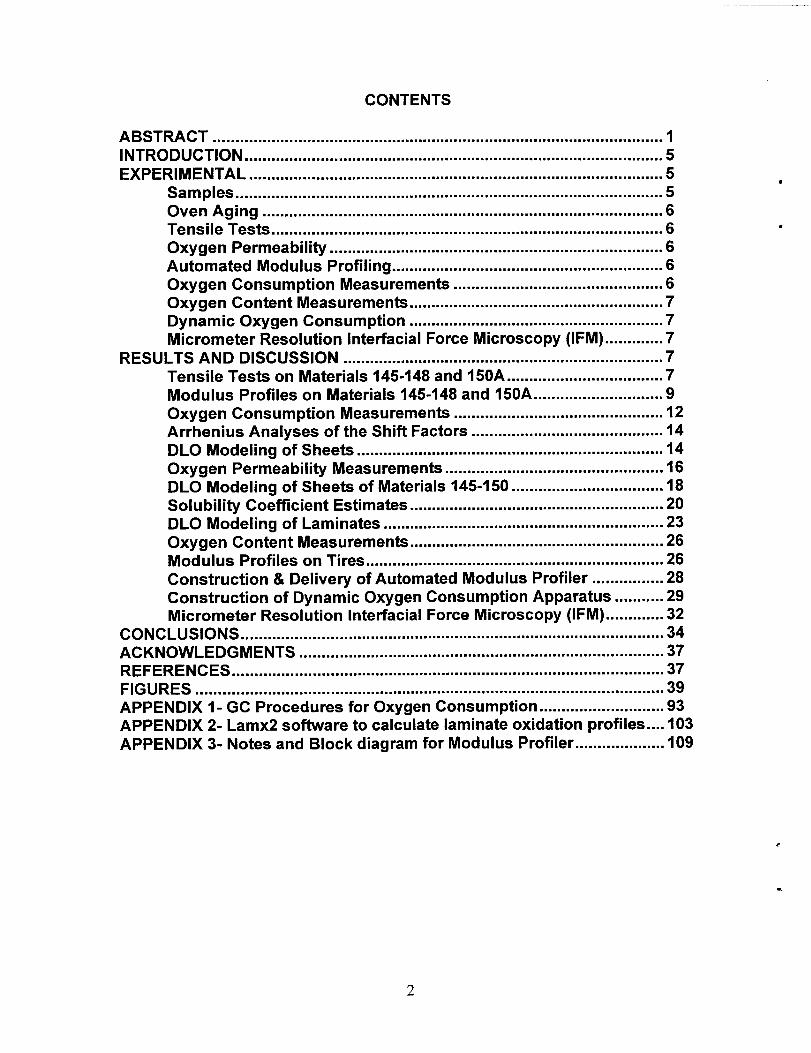
ABSTRACT ..................................................................................................... 1INTRODUCTION .............................................................................................. 5EXPERIMENTAL ............................................................................................. 5
Samples ................................................................................................ 5Oven Aging .......................................................................................... 6Tensile Tests ........................................................................................ 6Oxygen Permeability ........................................................................... 6Automated Modulus Profiling ............................................................. 6Oxygen Consumption Measurements ............................................... 6Oxygen Content Measurements ......................................................... 7
Dynamic Oxygen Consumption ......................................................... 7
Micrometer Resolution Interracial Force Microscopy (lFM) ............. 7RESULTS AND DISCUSSION ........................................................................ 7
Tensile Tests on Materials 145-148 and 150A ................................... 7Modulus Profiles on Materials 145-148 and 150A ............................. 9Oxygen Consumption Measurements ............................................... 12Arrhenius Analyses of the Shift Factors ........................................... 14DLO Modeling of Sheets ..................................................................... 14Oxygen Permeability Measurements ................................................. 16DLO Modeling of Sheets of Materials 145-150 .................................. 18Volubility Coefficient Estimates ......................................................... 20DLO Modeling of Laminates ............................................................... 23Oxygen Content Measurements ......................................................... 26Modulus Profiles on Tires ................................................................... 26Construction & Delivery of Automated Modulus Profiler ................28Construction of Dynamic Oxygen Consumption Apparatus ...........29Micrometer Resolution Interracial Force Microscopy (lFM) ............. 32
CONCLUSIONS ............................................................................................... 34ACKNOWLEDGMENTS .................................................................................. 37REFERENCES ................................................................................................. 37FIGURES ......................................................................................................... 39APPENDIX 1- GC Procedures for Oxygen Consumption ............................ 93APPENDIX 2- Lamx2 software to calculate laminate oxidation profiles .... 103APPENDIX 3- Notes and Block diagram for Modulus Profiler .................... 109
2

1 Nominal material compositions ................................................................... 52 Empirical shift factors for elongation data ................................................. 93 Unaged modulus results for Material 148 ................................................... 114 Unaged modulus results for Materials 145, 146 and 147 ........................... 115 Estimates of 02 consumption rates &02 permeability coefficients .........196 estimates of the parameter a assuming ß= 5............................................. 197 Time-dependent flux data for an EPDM material at 51 “C ........................... 218 Volubility coefficients for Materials 145-150 ............................................... 229 Parameters input into lamx2 program for 95°C aging of laminate ............ 2410 Parameters input into lamx2 program for 100°C aging of larger tire ...... 2511 Parameters input into lamx2 program for 70°C aging of smaller tire .....2512 Approximate width of apex region ............................................................. 2813 Dynamic versus static results for 40 mil samples of Material 154..........31

-This page intentionally left blank-
INTRODUCTION
This document highlights the important results obtained from the subtask of theGoodyear CRADA devoted to better understanding reliability of tires and to developingbetter lifetime prediction methods. The overall objective was toestablish the chemicaland physical basis for the degradation of tires using standard as well as unique modelsand experimental techniques. Of particular interest was the potential application of ourunique modulus profiling apparatus for assessing tire properties and for following tiredegradation. During the course of this complex investigation, extensive information wasgenerated, including experimental results, data analyses and development of models andinstruments. The purpose of this report is to summarize the most important aspects of thework. Some of the work was carried out using a combination of the Goodyear CRADAfunds and funds from the Enhanced Surveillance Program (ESP). Examples include thedevelopment of the ultrasensitive oxygen consumption technique, the improved oxygenpermeability capability and the construction of an interracial force microscope (IFM)capable of mapping mechanical properties with micrometer resolution. These and otherjoint developments therefore benefited and will continue to benefit the weapon programsas well as American industry in a synergistic manner.
EXPERIMENTAL
Samples
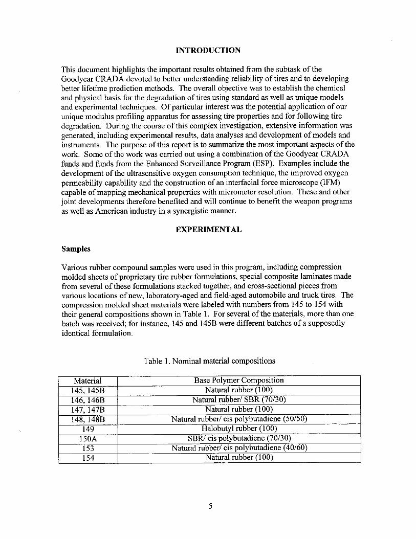
Various rubber compound samples were used in this program, including compressionmolded sheets of proprietary tire rubber formulations, special composite laminates madefrom several of these formulations stacked together, and cross-sectional pieces fromvarious locations of new, laboratory-aged and field-aged automobile and truck tires. Thecompression molded sheet materials were labeled with numbers from 145 to 154 withtheir general compositions shown in Table 1. For several of the materials, more than onebatch was received; for instance, 145 and 145B were different batches of a supposedlyidentical formulation.
Table 1. Nominal material compositions
Material Base Polymer Composition145, 145B Natural rubber (100)146, 146B Natural rubber/ SBR (70/30)147, 147B Natural rubber (100)148, 148B Natural rubber/ cis polybutadiene (50/50)
149 Halobutyl rubber (100)150A SBR/ cis polybutadiene (70/30)153 Natural rubber/ cis polybutadiene (40/60)154 Natural rubber (100)

Oven Aging
Oven aging of the tensile samples and the oxygen consumption containers was carried
out in air-circulating ovens (±1°C) equipped with thermocouples connected to continuousstrip chart recorders.
Tensile Tests
Tensile tests as functions of aging (time and temperature) were done on approximately0.2-cm thick samples of compounds 145, 146, 147, 148 and 150A and on approximately0.08 cm thick samples of compound 145. Before oven aging, strips approximately 6 mmwide by -150 mm long were cut from the compression molded sheets. Tensile testing(12.7 cm/min strain rate, 5.1 cm initial jaw separation) was performed using an Instronmodel 1000 testing machine equipped with pneumatic grips and having an extensometerclamped to the sample. This technique gave values of the ultimate tensile elongation, e,and the tensile strength at break, the latter reported as the value normalized to the unagedtensile strength at break.
Oxygen Permeability
Oxygen permeation measurements were performed on anOxtran-100 coulometricpermeation apparatus (Modern Controls, Inc., Minneapolis, MN, USA), which is basedon ASTM Standard D3985-81. Several modifications, the most important of which wasplacing the sample holder in an oven, have been made to this instrument to permit dataacquisition at higher temperatures (up to -95°C for the present studies) with minimal
temperature gradients (less than +0.5°C) across the sample during the experiment.Details on our new approach for obtaining oxygen permeability coefficients at hightemperatures in the presence of important oxygen consumption contributions will begiven in the Results and Discussion section below. This approach and the equipmentmodifications necessary for high temperature measurements were partially funded byboth this CRADA and the Enhanced Surveillance Program.
Automated Modulus Profiling
Modulus profiles with a resolution of -50 µm were obtained on sample cross-sectionsusing our modulus profiling apparatus, which has been described in detail previously [1-2]. This instrument measures inverse tensile compliance, which is closely related to thetensile modulus. A computer-controlled, automated version of this apparatus wasdeveloped for this CRADA. Details on this accomplishment will be given below in theResults and Discussion section.
Oxygen Consumption Measurements
This technique monitors the change in oxygen content caused by reaction with polymerin sealed containers using gas chromatographic detection. Since the development of the

approach was partially funded by this CRADA (jointly with the Enhanced SurveillanceProgram), details will be given later in the Results and Discussion section.
Oxygen Content Measurements
Oxygen content was determined as a function of radial position across the crown of thetire. Slices were prepared with Fortuna rubber slicing instrument. In rubber componentscontaining wires, slices were prepared with a scalpel. The slice depths (profile positions)were determined with calipers. Within each slice, five samples were taken. The oxygencontent data for each slice is an average of the five measurements. The typicalconfidence level is +/- 5°/0.
Oxygen content was measured with a LECO Oxygen Determinator (Model #RO-478).A sample of rubber about 2 milligram is charged into the furnace chamber and consumedat high temperature ( 1200°C) under nitrogen. The nitrogen sweeps the off-gases througha calibrated IR detector, which detects CO and CO2. The analysis determines the totalmolecular oxygen from the organic compounds in the rubber. Inorganic portions of therubber compound remain in the furnace as ash. An increase in oxygen content of an agedrubber compound would be a measure of oxidation.
Dynamic Oxygen Consumption
Since tires are deformed dynamically during the time when the bulk of the oxidativedegradation occurs, it would be useful to determine whether dynamic cycling duringaging increases the oxygen consumption rate relative to static aging conditions. Anapparatus capable of achieving this goal as well as having the capability of dynamicallyaging materials in rigorously anaerobic conditions, was developed for this program.Details on this apparatus and its capabilities will be given below in the Results andDiscussion section.
Micrometer Resolution Interracial Force Microscopy (IFM)
Since modulus profiling (50-µm resolution) proved extremely useful for studying theaging of tires and tire materials, it was concluded that having the capability of monitoringmechanical properties with even better resolution could lead to even more useful results.With this in mind, we began a program whose first goal was to produce an instrumentbased on building a modified IFM, capable of mapping mechanical properties ofmaterials with resolution of around 1-5 pm. The status of this work will be reviewed inthe Results and Discussion section below.
RESULTS AND DISCUSSION
Tensile Tests on Materials 145-148 and 150A
Materials 145-148 and 150A were aged in air-circulating ovens for various times at three
different temperatures (80°C, 95°C and 110°C). Typically, three samples were removed
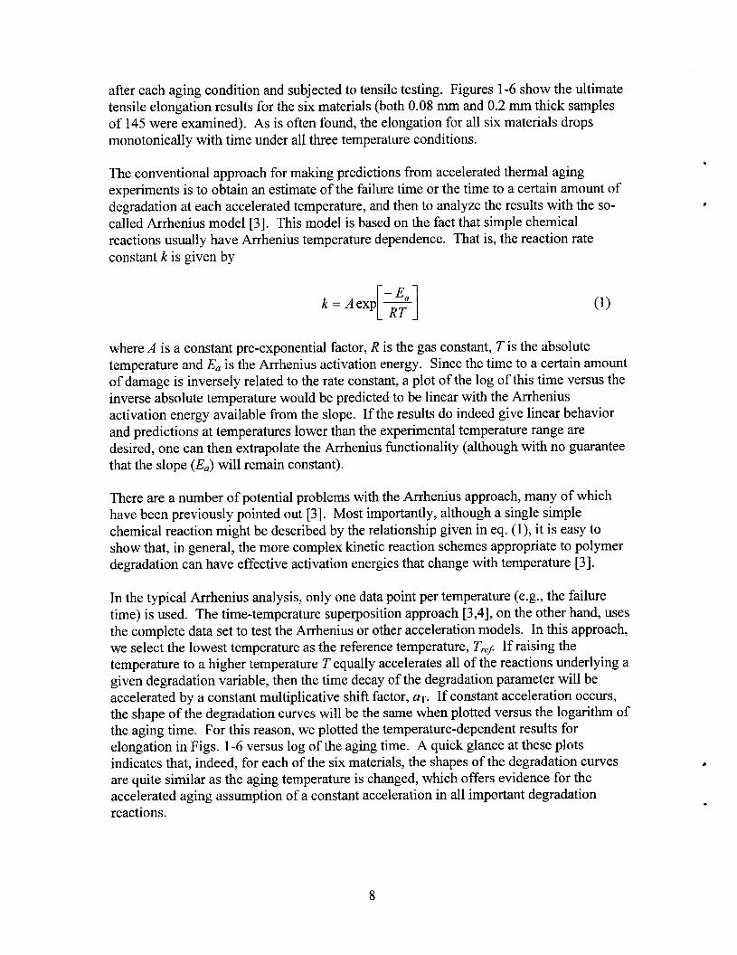
after each aging condition and subjected to tensile testing. Figures 1-6 show the ultimatetensile elongation results for the six materials (both 0.08 mm and 0.2 mm thick samplesof 145 were examined). As is often found, the elongation for all six materials dropsmonotonically with time under all three temperature conditions.
The conventional approach for making predictions from accelerated thermal agingexperiments is to obtain an estimate of the failure time or the time to a certain amount ofdegradation at each accelerated temperature, and then to analyze the results with the so-called Arrhenius model [3]. This model is based on the fact that simple chemicalreactions usually have Arrhenius temperature dependence. That is, the reaction rateconstant k is given by
[1k= Aexp ~ (1)
where A is a constant pre-exponential factor, R is the gas constant, T is the absolutetemperature and E. is the Arrhenius activation energy. Since the time to a certain amountof damage is inversely related to the rate constant, a plot of the log of this time versus theinverse absolute temperature would be predicted to be linear with the Arrheniusactivation energy available from the slope. If the results do indeed give linear behaviorand predictions at temperatures lower than the experimental temperature range aredesired, one can then extrapolate the Arrhenius functionality (although with no guaranteethat the slope (Q will remain constant).
There are a number of potential problems with the Arrhenius approach, many of whichhave been previously pointed out [3]. Most importantly, although a single simplechemical reaction might be described by the relationship given in eq. (1), it is easy toshow that, in general, the more complex kinetic reaction schemes appropriate to polymerdegradation can have effective activation energies that change with temperature [3].
In the typical Arrhenius analysis, only one data point per temperature (e.g., the failuretime) is used. The time-temperature superposition approach [3,4], on the other hand, usesthe complete data set to test the Arrhenius or other acceleration models. In this approach,we select the lowest temperature as the reference temperature, T,,y If raising thetemperature to a higher temperature T equally accelerates all of the reactions underlying agiven degradation variable, then the time decay of the degradation parameter will beaccelerated by a constant multiplicative shift factor, aT. If constant acceleration occurs,the shape of the degradation curves will be the same when plotted versus the logarithm ofthe aging time. For this reason, we plotted the temperature-dependent results forelongation in Figs. 1-6 versus log of the aging time. A quick glance at these plotsindicates that, indeed, for each of the six materials, the shapes of the degradation curvesare quite similar as the aging temperature is changed, which offers evidence for theaccelerated aging assumption of a constant acceleration in all important degradationreactions.
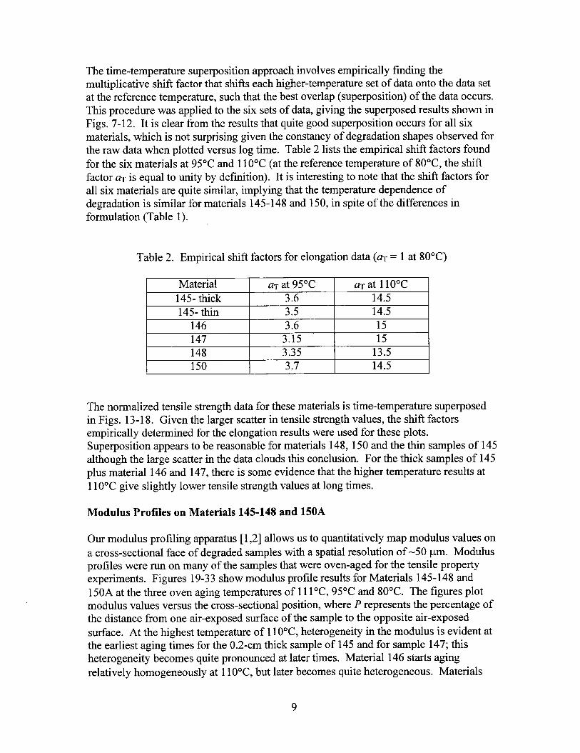
The time-temperature superposition approach involves empirically finding themultiplicative shift factor that shifts each higher-temperature set of data onto the data setat the reference temperature, such that the best overlap (superposition) of the data occurs.This procedure was applied to the six sets of data, giving the superposed results shown inFigs. 7-12. It is clear from the results that quite good superposition occurs for all sixmaterials, which is not surprising given the constancy of degradation shapes observed forthe raw data when plotted versus log time. Table 2 lists the empirical shift factors foundfor the six materials at 95°C and 110“C (at the reference temperature of 80”C, the shiftfactor aT is equal to unity by definition). It is interesting to note that the shift factors forall six materials are quite similar, implying that the temperature dependence ofdegradation is similar for materials 145-148 and 150, in spite of the differences informulation (Table 1).
Table 2. Empirical shift factors for elongation data (aT = 1 at 80”C)
Material aT at 95°C aT at 110”C145- thick 3.6 14.5145- thin 3.5 14.5
146 3.6 15147 3.15 15148 3.35 13.5150 3.7 14.5
The normalized tensile strength data for these materials is time-temperature superposedin Figs. 13-18. Given the larger scatter in tensile strength values, the shift factorsempirically determined for the elongation results were used for these plots.Superposition appears to be reasonable for materials 148, 150 and the thin samples of 145although the large scatter in the data clouds this conclusion. For the thick samples of 145plus material 146 and 147, there is some evidence that the higher temperature results at110“C give slightly lower tensile strength values at long times.
Modulus Profiles on Materials 145-148 and 150A
Our modulus profiling apparatus [1,2] allows us to quantitatively map modulus values ona cross-sectional face of degraded samples with a spatial resolution of -50 pm. Modulusprofiles were run on many of the samples that were oven-aged for the tensile propertyexperiments. Figures 19-33 show modulus profile results for Materials 145-148 and150A at the three oven aging temperatures of111°C, 95°C and 80°C. The figures plotmodulus values versus the cross-sectional position, where P represents the percentage ofthe distance from one air-exposed surface of the sample to the opposite air-exposed
surface. At the highest temperature of 110°C, heterogeneity in the modulus is evident atthe earliest aging times for the 0.2-cm thick sample of 145 and for sample 147; thisheterogeneity becomes quite pronounced at later times. Material 146 starts agingrelatively homogeneously at 110C, but later becomes quite heterogeneous. Materials
9
148 and 150A show relatively homogeneous aging behavior atll00C. The heterogeneitynoted for 145 and 147 (and later in time for 146) is caused by diffusion-limited oxidation(DLO). This occurs when the rate of consumption of the oxygen dissolved in a materialis faster than it can be replenished by diffusion from the surrounding air atmosphere. Asthe results indicate, a reduction in aging temperature leads to reduced DLO effects. Thisis because the oxygen consumption rate decreases more rapidly with decreasingtemperature than the oxygen permeation rate. Thus, all of the materials appear to age
relatively homogeneously when the aging temperature is reduced to 80”C.
Given the relative importance of DLO for several of the currently studied materials andthe complex way the importance of DLO changes with both time at higher temperaturesand with temperature, it is somewhat surprising that the ultimate tensile elongation resultsshow reasonable superposition for all of the materials. However, since oxidation at thesample surface will be the equilibrium oxidation expected under air-aging conditions(DLO effects are absent at the surface), the changes in modulus at the surface reflectoxidation in the absence of DLO. This observation coupled with the fact that the surfacemodulus increases with aging time faster than the modulus in interior regions indicatesthat the maximum rate of hardening occurs at the surface. When a sample is tensiletested, one might expect cracks to initiate first at the hardened surface. If such cracksimmediately propagate through the material, then the surface properties (equilibriumoxidation conditions) would determine the ultimate elongation. If this supposition is true,then a plot of surface modulus versus ultimate tensile elongation should be correlated forall aging temperatures. Such plots for the six materials, shown in Figs. 34-39, clearly
show that such a correlation exists (only 110°C profiles were obtained for the thin sampleof Material 145). Thus, the elongation is well behaved because the equilibrium oxidationat the sample surface determines the surface hardening which in turn determines theelongation. It is perhaps interesting to note that all of the materials reach fairly lowelongation values by the time the modulus has reached -100 MPa.
Tensile strength, which results from the same tensile test as elongation, might beexpected to behave quite differently since it comes from the force at break, a propertythat is integrated across the sample cross-section. As such, it should show evidence ofthe complex DLO effects as the temperature is changed unless the tensile strengthhappens to have little dependence on the level of oxidation. Even with the relativelylarge scatter in the tensile strength data, we saw earlier that the three materials withimportant DLO effects (thick 145, 146, and 147) gave indications of non-superposable
tensile strength data for long aging times at 110°C. Figure 40 shows a plot of elongationversus tensile strength for Material 147. The deviation of the data at 110“C reflects thefact that DLO reduces the tensile strength contributions for portions of the materialinfluenced by significant DLO effects.
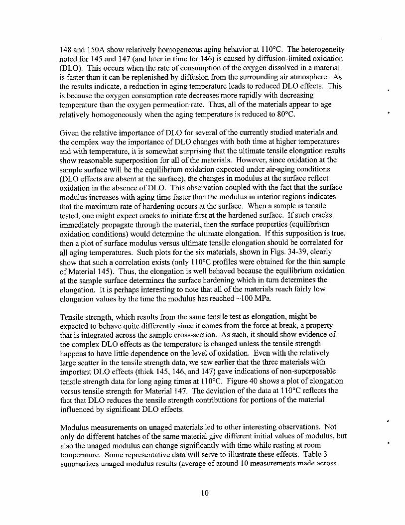
Modulus measurements on unaged materials led to other interesting observations. Notonly do different batches of the same material give different initial values of modulus, butalso the unaged modulus can change significantly with time while resting at roomtemperature. Some representative data will serve to illustrate these effects. Table 3summarizes unaged modulus results (average of around 10 measurements made across
10
sample using modulus profiling) for samples of Material 148 from several differentcompression molded sheets at different times and for samples of Material 148B (adifferent batch). The initial modulus measured for a sample from batch 148 was 3.4 MPain February, 1994. A repeat run on the exact same sample four and a half years later gavea modulus value of 4.5 MPa, an increase of approximate y 32%. Recent results on fourother sheets from this same batch gave values similar to the recently measured value.Recent results on thick and thin samples from batch 148B gave a slightly higher value(4.8 MPa).
Table 3. Unaged modulus results for Material 148.
Material Date Modulus, MPa
148 -sheet 1 2/8/94 3.4+().2
148 -sheet 1 (same sample) 8/27/98 4.5~0.2
148- sheet 2 8/27/98 4.34*0.15
148- sheet 3 8/27198 4.4+().4
148- sheet 4 8/27/98 4.13*0.15
148- sheet 5 8/27/98 4.4*0.3
148B- 0.08 cm 8/21/98 4.8~025
148B- 0.2 cm 8/21/98 4.8to.25
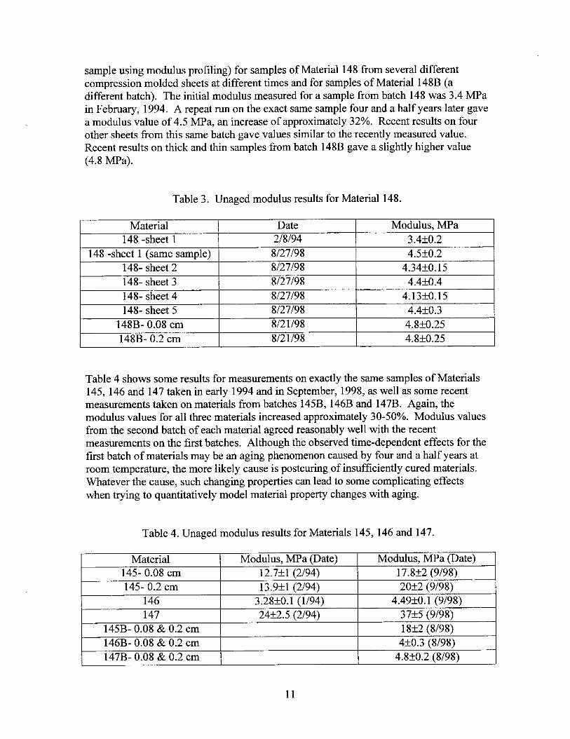
Table 4 shows some results for measurements on exactly the same samples of Materials145, 146 and 147 taken in early 1994 and in September, 1998, as well as some recentmeasurements taken on materials from batches 145B, 146B and 147B. Again, themodulus values for all three materials increased approximately 30-50%. Modulus valuesfrom the second batch of each material agreed reasonably well with the recentmeasurements on the first batches. Although the observed time-dependent effects for thefirst batch of materials maybe an aging phenomenon caused by four and a half years atroom temperature, the more likely cause is posturing of insufficiently cured materials.Whatever the cause, such changing properties can lead to some complicating effectswhen trying to quantitatively model material property changes with aging.
Table 4. Unaged modulus results for Materials 145, 146 and 147.
Material Modulus, MPa (Date) Modulus, MPa (Date)
145-0.08 cm 12.7+1 (2/94) 17.8*2 (9/98)
145- 0.2 cm 13.9+1 (2/94) 20+2 (9/98)
146 3.28+0.1 (1/94) 4.49*0.1 (9/98)
147 24*2.5 (2/94) 37*5 (9/98)
145B- 0.08 & 0.2 cm 18~ (8/98)
146B- 0.08 & 0.2 cm 4~0.3 (8/98)
147B- 0.08 & 0.2 cm 4.8+0.2 (8/98)
11

Oxygen Consumption Measurements
For several reasons, obtaining oxygen consumption results can bean invaluable aid tounderstanding both physical and chemical degradation phenomena. First of all, whenoxygen is available for reaction, oxidation reactions typically dominate the chemicaldegradation of elastomeric materials. We saw earlier that equilibrium oxidation at thesample surfaces of oven-aged materials leads to oxidative hardening which determinestensile elongation failure even in the presence of DLO effects. Another benefit of havingoxygen consumption results is that such results (in combination with oxygen permeabilityand volubility measurements) allow models to be developed and tested for determiningthe importance of DLO effects for both single materials and complex, compositestructures entailing several rubber layers of varying thicknesses. Eventually, suchapproaches should allow whole tires to be analyzed for the importance of oxidation andthe location of anaerobically aged regions during typical usage.
We perform our oxygen consumption measurements by sealing (using knife-edge flangesand a silver-plated copper gasket) known amounts of the material under investigationwith known amounts of oxygen in glass containers of known volume, typically 5-30 cc.Oxygen backfill pressures are chosen such that the starting pressure would be -16 cmHgat the temperature of the aging experiment (e.g., we allow for the pressure increase thatoccurs when the sample cell goes from ambient-temperature fill conditions to the agingtemperature). The containers are equilibrated for times greater than 2L2/D (L = samplethickness, D = oxygen diffusion coefficient within the sample) to assure that oxygendissolved in the sample is in equilibrium with the oxygen surrounding the sample.Additional oxygen is added as necessary to restore the gas pressure to the desired startingpressure. The containers are then thermally aged for time periods chosen to consume-40% of the oxygen (to make the average partial pressure during aging approximatelyequal to ambient conditions in Albuquerque (oxygen partial pressure -13.2 cmHg)).With appropriate choices of fill factors (fill factor= volume of sample/ gas volume incontainer) and time intervals, this technique can be used to measure oxygen consumptionrates down to -10-13 mol/g/s. This lower limit is achieved using fill factors of -50%, themaximum practical value, and time intervals of around 6 months.
After aging, the residual gas composition in the containers is measured directly using aHewlett-Packard model 5890 Series II Gas Chromatograph equipped with a thermalconductivity detector. External standards are used to setup a calibration scale for thegases being analyzed. At a single aging temperature, the container is run throughmultiple oxygen backfill/aging/analysis cycles, so that the oxygen consumption rates areobtained versus aging time.
Consumption rates of oxygen, ~, were calculated as
(2)
12
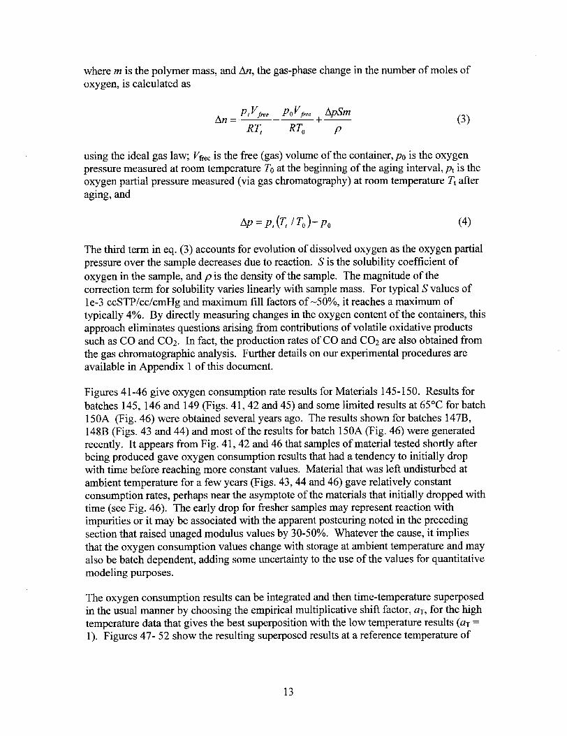
where m is the polymer mass, and An, the gas-phase change in the number of moles ofoxygen, is calculated as
P, Vf,.. POVf,,, + ApSmAn=
R~ – RTO p(3)
using the ideal gas law; Vf~~~is the free (gas) volume of the container, p. is the oxygenpressure measured at room temperature TOat the beginning of the aging interval, pt is theoxygen partial pressure measured (via gas chromatography) at room temperature Tt afteraging, and
(4)
The third term in eq. (3) accounts for evolution of dissolved oxygen as the oxygen partialpressure over the sample decreases due to reaction. S is the volubility coefficient of
oxygen in the sample, and P is the density of the sample. The magnitude of thecorrection term for volubility varies linearly with sample mass. For typical S values of1e-3 ccSTP/cc/cmHg and maximum fill factors of -50%, it reaches a maximum oftypically 4%. By directly measuring changes in the oxygen content of the containers, thisapproach eliminates questions arising from contributions of volatile oxidative productssuch as CO and C02. In fact, the production rates of CO and C02 are also obtained fromthe gas chromatographic analysis. Further details on our experimental procedures areavailable in Appendix 1 of this document.
Figures 41-46 give oxygen consumption rate results for Materials 145-150. Results for
batches 145, 146 and 149 (Figs. 41,42 and 45) and some limited results at 65°C for batch150A (Fig. 46) were obtained several years ago. The results shown for batches 147B,148B (Figs. 43 and 44) and most of the results for batch 150A (Fig. 46) were generatedrecently. It appears from Fig. 41, 42 and 46 that samples of material tested shortly afterbeing produced gave oxygen consumption results that had a tendency to initially dropwith time before reaching more constant values. Material that was left undisturbed atambient temperature for a few years (Figs. 43, 44 and 46) gave relatively constantconsumption rates, perhaps near the asymptote of the materials that initially dropped withtime (see Fig. 46). The early drop for fresher samples may represent reaction withimpurities or it may be associated with the apparent posturing noted in the precedingsection that raised unaged modulus values by 30-50%. Whatever the cause, it impliesthat the oxygen consumption values change with storage at ambient temperature and mayalso be batch dependent, adding some uncertainty to the use of the values for quantitativemodeling purposes.
The oxygen consumption results can be integrated and then time-temperature superposedin the usual manner by choosing the empirical multiplicative shift factor, aT, for the hightemperature data that gives the best superposition with the low temperature results (aT =1). Figures 47-52 show the resulting superposed results at a reference temperature of
13
65”C. The shift factors used to multiply the times at the higher temperatures are noted oneach of the figures.
Arrhenius Analyses of the Shift Factors
We can now take the empirically derived, multiplicative shift factors determined for theelongation results (Table 2) and for the oxygen consumption data (previous section) andplot the log of these results versus inverse absolute temperature. This plot will allow usto see whether Arrhenius behavior (linear results) is consistent with the oxidativedegradation of these materials. Since the elongation results were derived using 80°C asthe reference temperature, we adjust the oxygen consumption results from the previoussection so that 80”C corresponds to a shift factor of unity. For the oxygen consumption
results of Materials 147B, 148B and 150A, where 80”C was the upper temperature used,
this procedure simply requires dividing each shift factor by the 80”C shift factor. For the
other materials, where the upper temperature was 96.5”C, the numbers for 65°C and96.5°C were each divided by a constant such that the resulting straight line between themwas consistent with a shift factor of approximately unity at 80°C. Figures 53-57 showthe resulting Arrhenius plots for the five materials; within experimental uncertainty, all ofthe materials show Arrhenius behavior with very similar Arrhenius activation energies.Since we saw earlier that the surface modulus values are well correlated with theelongation results, we can now conclude that the same temperature dependence holds forthe underlying oxidation reactions, the material modulus and the elongation. In fact,essentially the same activation energy holds for all of these materials. It should be noted,however, that the activation energy for Material 149 (a halobutyl compound) is -20kcal/mol from the oxygen consumption results (tensile degradation studies were not doneon this material).
DLO Modeling of Sheets
Diffision-limited oxidation was the reason for the complex time and temperaturedependent modulus profiles shown earlier. For most polymeric materials, the presence ofdissolved oxygen during aging causes oxidation chemistry to dominate the degradation.If the rate at which dissolved oxygen is used by reactions is faster than the rate at which itcan be replenished by diffusion from the surrounding air-atmosphere, a reduction indissolved oxygen concentration will occur. This effect, which can lead to reductions inor elimination of oxidation in the interior regions of the material, is referred to asdiffusion-limited oxidation [5-7]. To model this effect, diffusion expressions must becoupled with oxidative reaction rate expressions. A particularly useful and generalkinetic rate expression is based on a variant of the basic autoxidation scheme (BAS),which has been utilized for more than 50 years [8-9] to describe the oxidation of organicmaterials. For stabilized materials, the simplified classical oxidation scheme can bewritten as follows [3]:
14

Classical oxidation scheme.
Initiation Polymer *R.
Propagation RO+OZ “ >ROz O
Propagation ROZO+RH~>ROzH+ R.
Termination R02 ●k4=k;(AH)
> Products
Termination R, “’k’(~) } Products
Branching R02H “ >2R0 +ROH + HOH
Analysis of this scheme under steady state conditions for the two radical species and theROOH concentration leads to the following expression for the oxygen consumption rate,
@
402]~=7=
C,[02]
1+ C2[02]
where
k,k2c,=—
k5
k,(k, –2kJC2= -
k,(k~ + k4)
(5)
(6)
(7)
By combining the expression for oxygen consumption, ~, given by eq. (5) with standarddiffusion expressions [1O], the theory for DLO of sheet material (thickness L) is easilyderived [5-7]. Assuming Fickian behavior plus time-independent values for@ and for theoxygen permeability coefficient, POX,a steady-state solution is obtained in terms of twoparameters, cxand (3,given by
C,L2~=—D
p= c2sp = C2[021,
(8)
(9)
15
where Cl and C2 are given respectively in eq. (6) and eq. (7), p is the oxygen partialpressure surrounding the sample, D and S are the oxygen diffusivity and volubilitycoefficients for the polymer (the permeability coefficient, P.. is the product of D and S)
and [02 ], represents the equilibrium oxygen concentration at the surface of the sample.
It is clear from eqs. (8)-(9) that F can be changed by changing the oxygen partial pressure
surrounding the sample, and that a is a geometry-sensitive parameter, which can bechanged by varying the sample thickness. Some representative theoretical oxidationprofiles in terms of these two parameters are shown in Fig. 58. Extensive experimentaltests on neoprene and nitrile rubber materials aged in thermoxidative environments [7]and a viton elastomer [11] and an EPDM elastomer [6] aged in radiation environmentshave quantitatively confirmed the above DLO models.
Oxygen Permeability Measurements
Further testing of the above model for diffusion-limited oxidation (DLO) on the currentsheet materials requires measurements of oxygen permeability coefficients in addition tooxygen consumption results. Since the permeability measurements are required at hightemperatures, we needed to significantly modify a commercial oxygen permeabilityapparatus (Mocon Oxtran 100). The manufacturer’s specifications for the instrument
stated an upper temperature limit of 60”C, but the design of the sample holder andtemperature control for the as-received commercial instrument was so limited that
temperature gradients across the sample were found to be greater than 20°C at 60”C.
Because of such severe temperature limitations, extensive modifications were made to thecommercial instrument. The first modification was to eliminate the commercial sampleholder and its totally inadequate temperature control approach in favor of a newlydesigned holder that was placed in an air-circulating oven. The inner workings of thenew sample holder are shown in Fig. 59. A disk shaped sample is sealed by compressingbetween the two plates shown in the Figure with nitrogen gas flowing on one side and gascontaining a selected percentage of oxygen flowing on the opposite side. Thecoulometric detector of the commercial instrument detects the amount of oxygen thatpermeates through the 3 inch working diameter of the sample. The sample holder alsoallows an inverted, cup-shaped container to be placed over the sealing area and sealedwith bolts (see outside holes in figure) and a copper gasket. By purging this containerwith flowing nitrogen, this arrangement can be used to limit the amount of oxygenpermeating from the edge region where the sample is compression-sealed. Since theentire sample cell is placed in the center of an oven, any desired temperature is available.In addition, the large thermal mass of the sample holder suggests fairly uniformtemperatures across the sample. This is confirmed by monitoring thermocouples that areplaced near the center of the sample region and in the area where purging is available(approximately one inch outside the sample diameter); these thermocouples typically readwithin 0.5°C of each other at temperatures up to 150”C.
By allowing measurements at higher temperatures, two new problems arose that had to bedealt with. The first had to do with the inherent limits of the coulometric detector. As
16
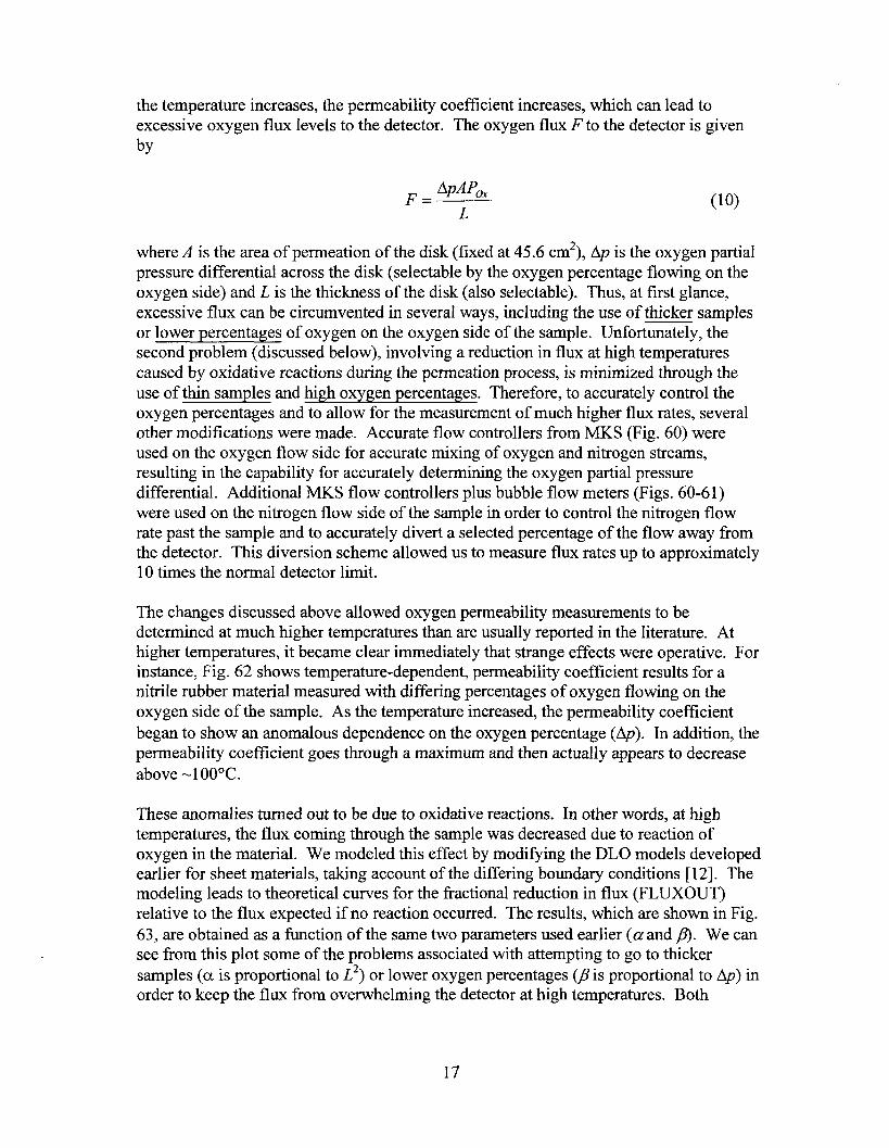
the temperature increases, the permeability coefficient increases, which can lead toexcessive oxygen flux levels to the detector. The oxygen flux F to the detector is givenby
ApAPoXF=
L(lo)
where A is the area of permeation of the disk (fixed at 45.6 cm2), Ap is the oxygen partialpressure differential across the disk (selectable by the oxygen percentage flowing on theoxygen side) and L is the thickness of the disk (also selectable). Thus, at first glance,excessive flux can be circumvented in several ways, including the use of thicker samplesor lower percentages of oxygen on the oxygen side of the sample. Unfortunately, thesecond problem (discussed below), involving a reduction in flux at high temperaturescaused by oxidative reactions during the permeation process, is minimized through theuse of thin samples and high oxygen percentages. Therefore, to accurately control theoxygen percentages and to allow for the measurement of much higher flux rates, severalother modifications were made. Accurate flow controllers from MKS (Fig. 60) wereused on the oxygen flow side for accurate mixing of oxygen and nitrogen streams,resulting in the capability for accurately determining the oxygen partial pressuredifferential. Additional MKS flow controllers plus bubble flow meters (Figs. 60-61)were used on the nitrogen flow side of the sample in order to control the nitrogen flowrate past the sample and to accurately divert a selected percentage of the flow away fromthe detector. This diversion scheme allowed us to measure flux rates up to approximately10 times the normal detector limit.
The changes discussed above allowed oxygen permeability measurements to bedetermined at much higher temperatures than are usually reported in the literature. Athigher temperatures, it became clear immediately that strange effects were operative. Forinstance, Fig. 62 shows temperature-dependent, permeability coefficient results for anitrile rubber material measured with differing percentages of oxygen flowing on theoxygen side of the sample. As the temperature increased, the permeability coefficient
began to show an anomalous dependence on the oxygen percentage (Ap). In addition, thepermeability coefficient goes through a maximum and then actually appears to decreaseabove -l OO°C.
These anomalies turned out to be due to oxidative reactions. In other words, at hightemperatures, the flux coming through the sample was decreased due to reaction ofoxygen in the material. We modeled this effect by modifying the DLO models developedearlier for sheet materials, taking account of the differing boundary conditions [12]. Themodeling leads to theoretical curves for the fractional reduction in flux (FLUXOUT)relative to the flux expected if no reaction occurred. The results, which are shown in Fig.63, are obtained as a function of the same two parameters used earlier (a and B. We cansee from this plot some of the problems associated with attempting to go to thickersamples (a is proportional to L2) or lower oxygen percentages @is proportional to Ap) inorder to keep the flux from overwhelming the detector at high temperatures. Both
17
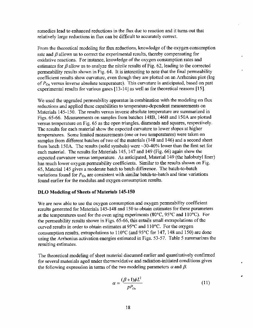
remedies lead to enhanced reductions in the flux due to reaction and it turns out thatrelatively large reductions in flux can be difficult to accurately correct.
From the theoretical modeling for flux reductions, knowledge of the oxygen consumptionrate and P allows us to correct the experimental results, thereby compensating foroxidative reactions. For instance, knowledge of the oxygen consumption rates and
estimates for ~ allow us to analyze the nitrile results of Fig. 62, leading to the correctedpermeability results shown in Fig. 64. It is interesting to note that the final permeabilitycoefficient results show curvature, even though they are plotted on an Arrhenius plot (logof POXversus inverse absolute temperature). This curvature is anticipated, based on pastexperimental results for various gases [13- 14] as well as for theoretical reasons [15].
We used the upgraded permeability apparatus in combination with the modeling on fluxreductions and applied these capabilities to temperature-dependent measurements onMaterials 145-150. The results versus inverse absolute temperature are summarized inFigs. 65-66. Measurements on samples from batches 148B, 146B and 150A are plottedversus temperature on Fig. 65 as the open triangles, diamonds and squares, respectively.The results for each material show the expected curvature to lower slopes at highertemperatures. Some limited measurements (one or two temperatures) were taken onsamples from different batches of two of the materials (148 and 146) and a second sheetfrom batch 150A. The results (solid symbols) were -30-40% lower than the first set foreach material. The results for Materials 145, 147 and 149 (Fig. 66) again show theexpected curvature versus temperature. As anticipated, Material 149 (the halobutyl liner)has much lower oxygen permeability coefficients. Similar to the results shown on Fig.65, Material 145 gives a moderate batch to batch difference. The batch-to-batchvariations found for POXare consistent with similar batch-to-batch and time variationsfound earlier for the modulus and oxygen consumption results.
DLO Modeling of Sheets of Materials 145-150
We are now able to use the oxygen consumption and oxygen permeability coefficientresults generated for Materials 145-148 and 150 to obtain estimates for these parametersat the temperatures used for the oven aging experiments (80°C, 95°C and 110“C). Forthe permeability results shown in Figs. 65-66, this entails small extrapolations of the
curved results in order to obtain estimates at 95°C and 110°C. For the oxygenconsumption results, extrapolations to 110°C (and 95°C for 147, 148 and 150) are doneusing the Arrhenius activation energies estimated in Figs. 53-57. Table 5 summarizes theresulting estimates.
The theoretical modeling of sheet material discussed earlier and quantitatively confirmedfor several materials aged under thermoxidative and radiation-initiated conditions givesthe following expression in terms of the two modeling parameters a and /?.
(P +l)@L2a.
Ppox
(11)
18
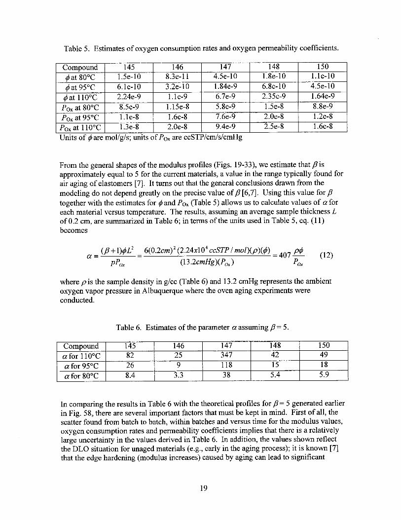
Table 5. Estimates of oxygen consumption rates and oxygen permeability coefficients.
Compound 145 146 147 148 150
~at 80°C 1.5e-10 8.3e-l 1 4.5e-10 1.8e-10 l.le-10
@at 95°C 6.le-10 3.2e-10 1.84e-9 6.8e-10 4.5e-10
@at 11O”C 2.24e-9 1.le-9 6.7e-9 2.35e-9 1.64e-9
POXat 80°C 8.5e-9 1.15e-8 5.8e-9 1.5e-8 8.8e-9
POXat 95°C 1.le-8 1.6e-8 7.6e-9 2.Oe-8 1.2e-8
POXat 110°C 1.3e-8 2.Oe-8 9.4e-9 2.5e-8 1.6e-8
Units of@ are mol/g/s; units of POXare ccSTP/cm/s/cmHg
From the general shapes of the modulus profiles (Figs. 19-33), we estimate that ~ isapproximately equal to 5 for the current materials, a value in the range typically found forair aging of elastomers [7]. It turns out that the general conclusions drawn from themodeling do not depend greatly on the precise value of ~ [6,7]. Using this value for #
together with the estimates for @and Pm (Table 5) allows us to calculate values of a foreach material versus temperature. The results, assuming an average sample thickness Lof 0.2 cm, are summarized in Table 6; in terms of the units used in Table 5, eq. (11)becomes
(B+ l)@L2 _ 6(0.2cnz)2 (2.24x10⁴ CCSTP/ ?YZOz)(~)(@)a. — .407@ (12)
Ppox (13.2crnHg)(Pox ) Pox
where p is the sample density in g/cc (Table 6) and 13.2 cmHg represents the ambientoxygen vapor pressure in Albuquerque where the oven aging experiments wereconducted.
Table 6. Estimates of the parameter a assuming ~= 5.
Compound 145 146 147 148 150
a for 110”C 82 25 347 42 49
a for 95°C 26 9 118 15 18
a for 800(7 8.4 3.3 38 5.4 5.9
In comparing the results in Table 6 with the theoretical profiles for P = 5 generated earlierin Fig. 58, there are several important factors that must be kept in mind. First of all, thescatter found from batch to batch, within batches and versus time for the modulus values,oxygen consumption rates and permeability coefficients implies that there is a relativelylarge uncertainty in the values derived in Table 6. In addition, the values shown reflectthe DLO situation for unaged materials (e.g., early in the aging process); it is known [7]that the edge hardening (modulus increases) caused by aging can lead to significant
19

reductions in POX,in turn leading to more and more important DLO effects. With thesepoints in mind, we can tentatively conclude from Table 6 that, from the very beginning ofaging, Material 147 at 110°C (a- 350) should show large DLO effects, and 147 at 95°C
(a- 120) and 145 at 110°C (a - 80) should show noticeable DLO effects. For all othercombinations of Materials and temperatures, degradation at early times should berelatively homogeneous. These conclusions are in reasonable accord with theexperimental modulus profiles shown in Figs. 19-33. For several combinations ofmaterial and aging temperature, the importance of DLO effects seems to grow at laterstages of the degradation; this is especially noticeable for 145 at 95°C and 146 at 110°C.Since we did not attempt to determine the effect of aging on the experimental values ofPOX,we cannot definitively conclude that decreases in l’ox are responsible for theseobservations.
Since Material 147 has the largest DLO effects, we will do a more complete comparisonof the experimental and theoretical profiles to show the general approach applied. Tocorrelate equilibrium oxidation to modulus, we use the surface modulus values versustime and temperature and superpose them in the usual manner, resulting in thesuperposed data shown in Figure 67. The shift factors used to superpose the data arevirtually identical to those used to superpose the elongation data (Fig. 10); this is notunexpected considering the correlation between surface modulus and elongation (Fig.37). The superposed data is plotted on a semi-log plot in order to see if the surfacemodulus grows approximately exponentially with time, a dependence observed forseveral other materials [7]. Although the superposed surface modulus data is not quiteexponential, we approximate the dependence by the exponential straight line shown onthe figure. Although this approximation is convenient for data analysis, morecomplicated functional forms can be easily handled in a similar fashion. Assuming that1) the oxidation follows this exponential behavior, 2) the oxygen consumption values andthe oxygen permeability coefficients do not change with aging and 3) the modelparameters estimated in Table 6 are accurate, theoretical modeling at the threetemperatures of interest leads to the results shown in Figs. 68-70. Comparing thesetheoretical results with the experimental results shown in Figs. 25-27 shows that ourunderstanding of DLO effects is quite reasonable. The comparisons imply that the valuesof a derived in Table 6 might be slightly high, but given the uncertainties in the valuescaused by batch to batch and time variations, any slight differences are easily explained.
Volubility Coefficient Estimates
Our next goal was to apply DLO modeling to a laminate containing numerous layers ofbonded rubbers, each of different thickness and with different oxygen consumption andpermeability coefficients. Developing such models is clearly required to eventuallyunderstand DLO effects for tire-like structures. For such composite, it turns out that anadditional parameter, the volubility coefficient (S), is needed for each layer in addition tothe oxygen consumption rates and the permeability coefficients.
Our first attempts to obtain estimates of volubility coefficients came from a method basedon measurement of pressure changes over time in a sealed container. For a commercial
20

EPDM elastomer (SR793B-80), the measured volubility obtained by this method was inclose agreement with literature values. However, for the natural rubber and SBR-basedelastomers under current study (Materials 145- 150), the solubilities derived greatlyexceeded literature values (by a factor of -5 for Materials 145-149 and a factor of-10 to15 for Material 150). Because we felt that this discrepancy with literature values calledinto question the derived values, we decided to use a second approach to estimate thevolubility coefficients. This approach uses the oxygen permeability apparatus to monitorthe time dependence of the oxygen flux. Before the experiment is started, nitrogen isflowed on both sides of the sample for sufficient time so as to assure that no oxygen isinitially in the sample. At time zero, the nitrogen flow on the oxygen side of the sampleis abruptly switched to oxygen flow. The oxygen flux detected on the coulometricdetector side of the sample is then monitored at selected times until equilibrium flux iseventually reached. The time dependent data allows both the volubility and diffusion (D)coefficients to be determined and therefore PO,, which is the product of S and D [16].The procedure involves plotting log[F’(tO’5)]versus L2/4t, where F is the flux, t is the timeand L is the sample thickness. The plot is predicted to give a straight line, with thediffusion coefficient available from the slope and the volubility coefficient available fromthe intercept. Representative data for a 0.201 cm thick disk of the EPDM elastomer (SR-793B-80) is given in Table 7 (AP = 6.6 cmHg).
Table 7. Time-dependent flux data foranEPDM material at51°C.
T, min F, ccSTP/m’/day Ft”’ L’14t
34 42.9 250 2.97e-454 70.4 517 1.87e-461 76.4 597 1.66e-4146 95.4 1153 6.92e-5256 97.6358 97.8
Figure 71 shows a plot of log[F’(i05)] versus L2/4t for this EPDM material. The datashow excellent linearity, which allows values for D and S (and therefore POX)to beobtained. The value of POXobtained (3 .45e-9 ccSTP/cm/s/cmHg) is virtually identicalwith the value obtained directly from the equilibrium flux at the end of the experiment(3.44e-9). In addition, the value of D can be obtained in another way as
L=D=—
6t 0.614
(13)
where tO.GIAis the time required for the flux to reach 61 .4°A of its equilibrium value [17].Using this approach, D is estimated to be 2.47e-6 cm2/s, again virtually identical to thevalue obtained from the analysis of Fig. 71 (2.48 e-6). Finally, the value of S derivedfrom Fig. 71 (1 .39e-3 ccSTP/cc/cmHg) is close to expected literature values for EPDM
21
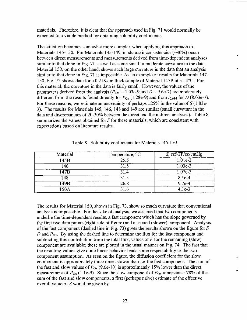
materials. Therefore, it is clear that the approach used in Fig. 71 would normally beexpected to a viable method for obtaining volubility coefficients.
The situation becomes somewhat more complex when applying this approach toMaterials 145-150. For Materials 145-149, moderate inconsistencies (-30%) occurbetween direct measurements and measurements derived from time-dependent analysessimilar to that done in Fig. 71, as well as some small to moderate curvature in the data.Material 150, on the other hand, shows such large curvature in the data that an analysissimilar to that done in Fig. 71 is impossible. As an example of results for Materials 147-150, Fig. 72 shows data for a 0.218-cm thick sample of Material 147B at 31.4”C. Forthis material, the curvature in the data is fairly small. However, the values of theparameters derived from the analysis (Pox - 1.03e-9 and D - 9.6e-7) are moderatelydifferent from the results found directly for POX(1 .28e-9) and from to,(jlafor D (8.03e-7).
For these reasons, we estimate an uncertainty of perhaps ±25% in the value of S (1.03e-3). The results for Materials 145, 146, 148 and 149 are similar (small curvature in thedata and discrepancies of 20-30% between the direct and the indirect analyses). Table 8summarizes the values obtained for S for these materials, which are consistent withexpectations based on literature results.
Table 8. Volubility coefficients for Materials 145-150
Material Temperature, “C S, ccSTP/cc/cmHg
145B 25.5 1.Ole-3
146 31.5 1.03e-3
147B 31.4 1.07e-3
148 31.5 8.le-4149B 26.8 9.7e-4150A 31.6 4.le-3
The results for Material 150, shown in Fig. 73, show so much curvature that conventionalanalysis is impossible. For the sake of analysis, we assumed that two componentsunderlie the time-dependent results, a fast component which has the slope governed bythe first two data points (right side of figure) and a second (slower) component. Analysisof the fast component (dashed line in Fig. 73) gives the results shown on the figure for S,D and POX. By using the dashed line to determine the flux for the fast component andsubtracting this contribution from the total flux, values off’ for the remaining (slow)component are available; these are plotted in the usual manner on Fig. 74. The fact thatthe resulting values give quite linear behavior lends some respectability to the two-component assumption. As seen on the figure, the diffusion coefficient for the slowcomponent is approximately three times slower than for the fast component. The sum ofthe fast and slow values of PoX (9.6e-10) is approximately 15% lower than the directmeasurement of POX(1.1e-9). Since the slow component of POXrepresents -78% of thesum of the fast and slow components, a first (perhaps naive) estimate of the effectiveoverall value of S would be given by
22

S = (0.78)(5.06e –3) + (0.22)(4 .8e–4) = 4.le –3
This value is approximately four times larger than both values of S for the other materialsand typical literature results. Given the large curvature observed in Fig. 73 coupled withthe speculative manner in which we derived an effective value for S, this result (shown inTable 8) should be viewed with caution. Clearly, the behavior of Material 150 is non-classical (non-Fickian). Although the other five materials show minor hints of unusualbehavior, to a first approximation, we can assume that they follow classical behavior.
DLO Modeling of Laminates
The DLO modeling of single sheet material was extended to laminated sheets of material.For each layer, kinetic expressions based on the earlier-introduced oxidation chemistrywere assumed to be valid. In addition the usual assumptions made in such modeling wereinvoked (e.g., Fickian diffusion, Henry’s Law, steady-state conditions). Since constantflux must be invoked at boundaries between sheets, an additional parameter (thevolubility coefficient S,) is needed for each layer. A program called lamx2, based on themodeling, was written and delivered to Goodyear. A copy of this program is included inAppendix 2. The program calculates profiles for the oxygen concentration and relativeoxidation rate in laminates up to 20 layers, each layer having different thickness, oxygenconsumption rate, oxygen permeability coefficient, oxygen volubility parameter andvalue for the parameter ~ defined in eq. (9). Calculations are solved numerically with therelative oxidation in each inner layer calculated as if that specific layer were at thesurface.
An attempt to test the laminate DLO model was done on a specially prepared laminatesupplied by Goodyear. This laminate was prepared by curing five sheets of differentthicknesses (each sheet had a uniform thickness) together. The position and thickness ofeach layer and the overall laminate thickness were meant to represent the crown area of atire. The first two columns of Table 9 give the materials used for each layer and theirthickness as a percentage of the overall sample. Figure 75 shows modulus profilingresults for the laminate as received. Also plotted (solid lines) are the expected modulusvalues based on the “equilibrium” values found for the individual materials (see Tables 3and 4). It is clear from the modulus profiles that the material properties of the layerschange substantially when cured as a laminate; similar effects would clearly beanticipated for actual tires. Since internal compounds (e.g., 145) use increased levels ofsulfur to improve adhesion to steel belts, transfer of excess sulfur across the variousinterfaces during cure may be one of the reasons for such effects. The apparentundercuring effect, mentioned earlier for individual sheet materials, could be animportant reason for the overall reductions in the laminate modulus values versus theexpected single sheet results.
23
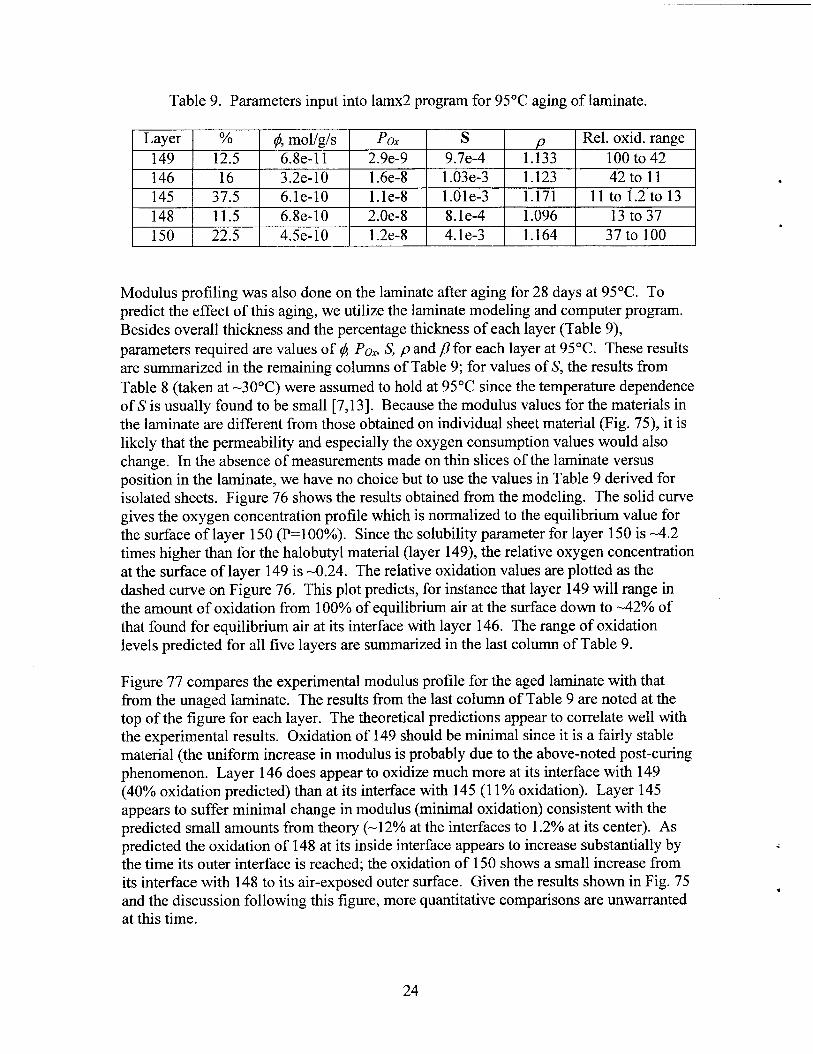
Table 9. Parameters input into lamx2 program for 95°C aging of laminate.
Layer ‘xO ~, mollgls Pox s P Rel. oxid. range
149 12.5 6.8e-l 1 2.9e-9 9.7e-4 1.133 100 to 42146 16 3.2e-10 1.6e-8 1.03e-3 1.123 42toll145 37.5 6.le-10 1.le-8 1.Ole-3 1.171 lltol.2to13148 11.5 6.8e-10 2.Oe-8 8.le-4 1.096 13t037150 22.5 4.5e-10 1.2e-8 4.le-3 1.164 37to 100
Modulus profiling was also done on the laminate after aging for 28 days at 95”C. Topredict the effect of this aging, we utilize the laminate modeling and computer program.Besides overall thickness and the percentage thickness of each layer (Table 9),
parameters required are values of 4 Po., S, p and ~ for each layer at 95”C. These resultsare summarized in the remaining columns of Table 9; for values of S, the results fromTable 8 (taken at -30°C) were assumed to hold at 95°C since the temperature dependenceof S is usually found to be small [7,13]. Because the modulus values for the materials inthe laminate are different from those obtained on individual sheet material (Fig. 75), it islikely that the permeability and especially the oxygen consumption values would alsochange. In the absence of measurements made on thin slices of the laminate versusposition in the laminate, we have no choice but to use the values in Table 9 derived forisolated sheets. Figure 76 shows the results obtained from the modeling. The solid curvegives the oxygen concentration profile which is normalized to the equilibrium value forthe surface of layer 150 (P=l00%). Since the volubility parameter for layer 150 is -4.2times higher than for the halobutyl material (layer 149), the relative oxygen concentrationat the surface of layer 149 is -0.24. The relative oxidation values are plotted as thedashed curve on Figure 76. This plot predicts, for instance that layer 149 will range inthe amount of oxidation from 10O% of equilibrium air at the surface down to -42% ofthat found for equilibrium air at its interface with layer 146. The range of oxidationlevels predicted for all five layers are summarized in the last column of Table 9.
Figure 77 compares the experimental modulus profile for the aged laminate with thatfrom the unaged laminate. The results from the last column of Table 9 are noted at thetop of the figure for each layer. The theoretical predictions appear to correlate well withthe experimental results. Oxidation of 149 should be minimal since it is a fairly stablematerial (the uniform increase in modulus is probably due to the above-noted post-curingphenomenon. Layer 146 does appear to oxidize much more at its interface with 149(40% oxidation predicted) than at its interface with 145(11% oxidation). Layer 145appears to suffer minimal change in modulus (minimal oxidation) consistent with thepredicted small amounts from theory (-12% at the interfaces to 1.2% at its center). Aspredicted the oxidation of 148 at its inside interface appears to increase substantially bythe time its outer interface is reached; the oxidation of 150 shows a small increase fromits interface with 148 to its air-exposed outer surface. Given the results shown in Fig. 75and the discussion following this figure, more quantitative comparisons are unwarrantedat this time.
24

Another example of the use of the laminate modeling program involves its application toreal tires. We can select a given type of tire and use the program to estimate theimportance of DLO effects at a given location by approximating the cross-section at thatlocation as a laminate made up of constant thickness layers representative of the rubberlayer thicknesses at that location. We can then input the required variables. For instance,
for atypically constructed larger size tire at an “operating” temperature of 100”C, theestimated parameters for a cross-section ending at the groove of the tread would be givenby the results shown in the first six columns of Table 10. Inputting these parameters into
lamx2, using ~ = 5, an oxygen cavity pressure of 125 cmHg and an external oxygenpressure of 15 cmHg, leads to the results shown in Fig. 78. A summary of the relativeoxidation ranges (relative to equilibrium oxidation under ambient air (15cmHg ofoxygen)) for each layer is given in the last column of Table 10. It is clear from theseresults and from Fig. 78 that a large percentage of layer 147 is predicted to age underanaerobic conditions.
Table 10. Parameters input into lamx2 program for 100”C aging of a larger size tire.
Layer 0/0 f$, mollgls Pox s P Rel. oxid. range
149 11 1.06e-10 3.4e-9 9.7e-4 1.133 222 to 98145 5 9.5e-10 1.2e-8 1.Ole-3 1.171 98 to 50147 73 2.86e-9 8.2e-9 1.07e-3 1.195 50 to Oto 29
I 1 I 1 1 1
150 11 7e-10 1.3e-8 4.le-3 1.164 29 to 100 I
For a typically constructed smaller size tire at an “operating” temperature of 70”C, theestimated parameters for a cross-section ending at the groove of the tread would be givenby the results shown in the first six columns of Table 11. Inputting these parameters into
lamx2, using P = 5, an oxygen cavity pressure of 51 cmHg and an external oxygenpressure of 15 cmHg, leads to the results shown in Fig. 79. In this instance, the lowertemperatures coupled with the thinner cross-sectional distance, leads to some drop in theoxidation levels for the internal layers but not anaerobic conditions.
Table 11. Parameters input into larnx2 program for 70”C aging of a smaller size tire,
Layer !YO ~, mollgls Pox s P Rel. oxid. Range*
149 11 6.2e-12 1.2e-9 9.7e-4 1.133 140 to 94146 12 3.2e-l 1 9e-9 1.03e-3 1.123 94 to 76148 15 6.9e-11 1.2e-8 8.le-4 1.096 76t061145 41 5.5e-11 7e-9 1.Ole-3 1.171 61 to 50to 69150 21 4e-11 6.6e-9 4.le-3 1.164 69 to 100
25

Constant temperatures were used for the above calculations on the two tires. In reality,temperature distributions occur across the cross-section, with higher temperatures ininternal regions and lower temperatures in other areas (clearly the surface of the treadwill be close to ambient outside temperature). Thus a more precise estimate of theimportance of DLO effects would have to consider the actual temperature distributions inthe tire. In principal, such complications can be handled by writing a more sophisticatedprogram that breaks each layer up into a multitude of sub-layers, each with the proper
temperature-dependent values of ~, Po. and S. However, since the purpose of thecalculations is to get approximate estimates of the importance of DLO effects and areaswhere anaerobic aging is likely, such an extension is not really called for. In addition, thechanges that would result from a more sophisticated attempt to account for thetemperature variations across the tire versus the use of a weighted-average temperaturewould probably not be large.
Modeling such as that done above for the larger tire (Fig. 78 and Table 10) representedthe second piece of evidence suggesting that important anaerobic aging effects werelikely for internal rubber materials in heavier tires. The first indications of theimportance of such anaerobic effects came from modulus profiling results (to bedescribed below). This insight, which was later confirmed by oxygen content analyses atGoodyear (next section), represented one of the most important accomplishments of thisCRADA. It has led to a radical reordering of research directions at Goodyear. Currentlyat Goodyear, there is a heavy emphasis on anaerobic aging effects, an area of researchthat was hardly being looked at prior to the discoveries made in this CRADA.
Oxygen Content Measurements on New and Worn Tires
To help understand the importance of anaerobic aging on the internal rubber componentsof heavier tires, oxygen content was determined on new and worn tires. The change ofoxygen content during tire testing would provide direct evidence of oxidation incomponents of interest. The oxygen content radial profiles of the crown area of a newtire and a lab-tested tire are shown in Figure 80. A new tire and a lab-tested tire with thesame construction were dissected. Small pieces (-2 mg) across the crown area wereanalyzed. The difference in oxygen content as a function of position is shown in Figure81. The internal components did not change in oxygen content, indicating anaerobicconditions. The external components (0-1 5 relative position) increased in oxygencontent, indicating oxidation. A road-tested (in-service) tire was analyzed in a similarfashion (Figure 82). The internal components (15-65 relative position) did not change inoxygen content, indicating anaerobic conditions (Figure 83). The external components(0-1 5 and 65-100 relative position) experienced oxidation.
Modulus Profiles on Tires
Our modulus profiling apparatus is capable of quickly (-1 minute per modulusmeasurement) and easily measuring modulus values with approximately 50 µmresolution and typically ±5% reproducibility. It became evident very early in thisCRADA that modulus profiling of tire cross-sections led to unique, interesting and
26

extremely valuable information. For this reason, Sandia ran numerous modulus profileson various locations of new, laboratory-aged, and field-aged tires supplied by Goodyear.A few representative examples will be described in this section.
Figure 84 compares modulus profile results for an unaged and an aged small tire at thetread-sidewall intersection area. The first thing to note is the richness of informationimmediately available from the modulus profiling technique. In the tread region of theunaged sample, the modulus is relatively constant. This is not the case, however, acrossseveral of the internal layers. As discussed earlier, this is probably due to such things assulfur transfer between layers during cure. With aging, the modulus values tend toincrease at all locations in the cross-section, consistent with the oxidation results notedearlier for the various sheet materials. This is consistent with modeling expectations forthese tires, where small to moderate DLO effects are expected for internal layers, butanaerobic aging is not anticipated. The increase in the tread area is fairly uniform,indicating relatively constant oxidation. Further into the tire cross-section, the increasesdrop indicating reductions in oxidation. At about 3 mm from the inside of the tire, littlechange in modulus occurs, suggestive perhaps of moderate to important DLO effects.
The same richness of information is immediately observed in Fig. 85, which gives resultsfor an unaged and an aged tire sidewall. Although aging in this instance leads to onlyminor increases in modulus, the technique does show that a substantial hardening occursat the surface of the sidewall exposed to outside ambient air.
The results for a larger tire, summarized in Fig. 86, are quite different from the tire resultsshown above. The first thing to notice is that the layers of the unaged tire have fairlyuniform modulus values, implying less washing out of the differences between layerscaused by such things as sulfur transfer during cure. More remarkable, however, is theobservation that aging tends to lead to reductions in modulus values for all of the internallayers. Since anaerobic aging conditions are expected in such regions, this suggests thatanaerobic aging may lead to sufficient reversion so as to reduce the modulus of thesematerials. In the layer adjacent to the tread (-1 0-14 mm), the drop is more severe awayfrom the tread interface. It is likely that some oxidation is occurring at the tread interfaceand that the amount of oxidation drops towards the other side of this layer. Similareffects may be operative in the region from -3 to 6 mm.
Experiments that focussed on the tread region of tires showed for the first time thatslightly enhanced oxidation was occurring at the tread surface of an aging tire. Figure 87gives atypical result. For these experiments, two pieces of the material were placed inour modulus profiling sample holder with their tread surfaces pressed together (facingeach other). The point of contact of the tread surfaces was defined as Omm. Asindicated in the figure, the modulus increases (typically by about 20-40°/0) at the treadsurface. This indicates a connection between the amount and depth of oxidativehardening of the surface material and the tread life, implying a potential method foroptimizing the tread formulation against wear. Experiments at Goodyear are in theprocess of evaluating the correlation between surface oxidation and abrasion properties oftire materials.
27

Because of the resolution capability of the modulus profiling apparatus, it can be used tomake measurements that are extremely difficult or impossible by other approaches. Forinstance, in the above tire profiles, this capability allowed measurements to be made inregions not previously accessible, such as between steel cords or in small regionsbetween belts. In another such application, studies were conducted in the apex regions ofexperimental tires manufactured by Goodyear. Figure 88 shows a crude sketch of thecross-section of the apex region of a tire designated as ER1001. The apex regioncomprises a relatively hard elastomer in the central triangular-like region whose basestarts near the bead. The region is -76 mm in length; its width variation is shownapproximately in Table 12.
Table 12. Approximate width of apex region
Distance from tip end, mm 1 5 12 17 42 76 (near bead)Width, mm 0.4 0.6 0.7 1.3 3 6.5
Modulus profiles were run on an unaged cross-section (sample 1001-31) and a samplefrom a tire run under severe handling maneuver conditions (ER1001 - 10). The profileswere taken along the approximate centerline of the apex region, starting at the bead (P=0%) and proceeding to the narrow tip (P = 100%). The results for both samples areshown in Fig. 89. Although aging has little effect on the properties, the modulus valuesfor the apex material vary dramatically dependent upon the position in the apex region.Values start at around 30 MPa near the bead, rising slightly to 40-45 MPa in the centerregion, then dropping substantially to around 10 MPa near the tip. This most likelyindicates under curing in the low modulus tip region. Figure 90 shows a modulus profileperpendicular to the apex direction at a distance of -6 mm from the apex tip. The widthof the apex region at this location is approximately 0.6 mm. The approximately constantvalues of modulus across the apex region indicates both a uniformly cured material at thislocation and shows that the low-modulus, adjacent material is not influencingmeasurements in the narrow apex region. These results also imply that transfer ofconstituents (e.g., sulfur) across boundary layers during cure does not account for thereduction in modulus for the apex material near its tip.
Construction and Delivery of Automated Modulus Profiler
It became clear from the results of the previous sections that data from our modulusprofiling apparatus represented unique and extremely useful information on tires and tirematerials. Because Goodyear was interested in running large numbers of samples on theinstrument, they eventually requested that we build and deliver a second apparatus fortheir in-house use. Our original instrument was designed for occasional use and involvedfull-time, tedious attention by an operator during data acquisition. Given the number ofsamples that Goodyear expected to run, it was necessary to modify the apparatus so that itwas completely automated and computer-controlled before delivery to Goodyear. This
28

upgrade would not only allow Goodyear to conveniently run numerous samples, but asimilar automation of our existing instrument would result in a significant improvementin capabilities for our work on Defense programs.
For each modulus measurement, the original instrument involved manual placement ofthe contact load, followed by manual addition of the major load 30 seconds later. Aftermanually recording the difference in penetration caused by the two loads, the loads werethen manually removed from the sample, the sample manually moved to the nextmeasurement location and the process repeated until all measurements were finished.Clearly, full-time attention by an operator was required. Using stepper motors, stepperdrivers and associated electronic controls together with a Pentium computer and LabTechSoftware, all of these manual operations were converted to automated control. Inaddition, the computer was utilized to 1) select the number and distance between datapoints, 2) acquire and analyze the data, and 3) control the temperature of the silicone oilbath used to stabilize the zero-weight float position. More details are given in Appendix3, which contains instructions for the use of the computer-controlled instrument, plustiming, block diagrams and associated information on the modifications.
Two modified instruments were successfully completed and then extensively tested onGoodyear and weapon-related samples. One of the modified instruments was kept atSandia. The other was delivered to Goodyear in late, 1996 after Goodyear personnelwere trained k its use at Sandia. Figure 91 shows a picture of Sandia’s completedapparatus, with a closer view of the sample area shown in Fig. 92. A typical computeroutput of the raw data (lower plot) and the analyzed modulus profile (upper plot) areshown in Fig. 93. Over the past year or so, Goodyear has used their apparatus soextensively that they are now running profiles 8 hours per day and claim to have a 2-yearbacklog of samples that they would like to examine. For this reason, they recentlyrequested that we build them a second apparatus using funds-in Goodyear money. Weare expecting to deliver the second instrument in early, 1999.
Construction of Dynamic Oxygen Consumption Apparatus
We saw earlier that important diffusion-limited oxidation (DLO) effects can occur in tirecross-sections, leading to reductions in oxidation and even aging under anaerobicconditions for internal tire layers. We also saw that it is possible to model these effectsusing knowledge of oxygen consumption, oxygen permeability and oxygen volubilityparameters for each layer. Since the oxidation and aging of tires occurs predominantlywhen the tire is moving, one important question for such modeling is the possible effectof dynamic strain on these parameters. Although it is unlikely that dynamic strain effectspermeability and volubility coefficients, it could have an effect on the oxygenconsumption rates. Since no one has ever attempted to address this issue, we decided tobuild an apparatus that would allow us to answer this question.
The construction of such an instrument offers an immediate challenge since the dynamicstraining must be accomplished in conjunction with the high vacuum requirement neededfor the GC approach to oxygen consumption measurements. We achieved a workable
29

approach utilizing a metal bellows welded to a can (Fig. 94) that could be vacuum-sealedusing copper gaskets on knife-edge metal seals. By connecting the metal bellows to amotor and cam arrangement (Fig. 95), it was possible to sinusoidally strain multipletensile specimens (at 3.5 Hz) attached internally to the bellows (Fig. 96). In addition tooxygen consumption capabilities, the vacuum-tight capabilities of the instrument allow usto dynamically age samples under rigorously controlled atmospheric conditions. Thismeans that samples can be dynamically exposed under true anaerobic conditions.
Preliminary tests on the original design uncovered several problems, which led to designchanges and improvements in the apparatus. For instance, the original design used onecentrally located motor to drive the bellows for both cells. The forces were balanced atthe start of the experiment by proper horizontal positioning of the motor. Unfortunately,if the aging of samples in one of the two cells was faster than the samples in the othercell, the balance was lost over time, leading to mechanical instability. Building twoseparately controlled systems eliminated this problem. Another important change in thedesign was to add a solid cylinder to fill void space internal to the strained samples (Fig.96). This reduced the free gaseous volume inside the can from -1000 cc to 420 cc,effectively increasing the sensitivity of the apparatus by -2.5 times and thereby allowingexperiments under selected conditions of sample mass plus temperature to be done -2.5times faster. Another problem involved fairly large temperature gradients across thesample containers. This was minimized by adding air-flow baffling to divert hot air-flowfrom the bottom of the cells and suspending the cells from the top of the oven to avoidthermal contact with the oven bottom (Fig. 94). Another modification was to change theholder arrangement from ten 6-mm wide samples to six 12-mrn wide samples (Fig. 96),so that 10-mm disks could be cut from the samples after aging for subsequent dynamicproperty evaluations at Goodyear.
Our first set of experiments using the more sensitive arrangement (free volume Vf= 420cc) were run on 80-mil thick samples of Material 153 at a temperature of -72”C.Duplicate runs in the two dynamic cells were compared to simultaneously run duplicateexperiments under static conditions. The static cells were attached to the side of thedynamic cells as illustrated in Fig. 94. Under these conditions, we measured oxygenconsumption rates of around 2e-10 mol/g/s for both types of samples. Unfortunately, thisresult implies that oxygen consumption measurements on 80 mil thick samples may beinfluenced by DLO effects, thereby necessitating thinner samples for the measurements.This can be seen by using an approximate relationship that gives the critical thickness L.for the beginning of important DLO effects [6].
[13PPOX0.5
Lc=—4
(14)
where the parameters p, PO, and @have the same meanings as earlier. With Albuquerquepartial pressure p of oxygen equal to 13.2 cmHg, Po. typically around 5e-9ccSTP/cm/s/cmHg and @equal to 2e- 10 mol/g/s, this equation leads to an L. of 76 roil.Therefore, at -70”C, we are forced to use 40 mil thick samples to assure ourselves that
30

DLO effects are not influencing the results. For other samples and temperature
conditions, similar calculations can be made using the measured value of $ together withmeasurements or estimates of POXin order to judge the potential importance of DLOeffects to the measurement.
Suppose we are trying to make measurements corresponding to Albuquerque ambientoxygen pressure conditions. We therefore want the average oxygen pressure in thecontainer to be -13.2 cmHg at the aging temperature. During the experiment, we needthe drop in oxygen pressure to be large enough to accurately measure (4 cmHg isreasonable), implying starting at -15.2 cmHg and ending up at -11.2 cmHg. If the aging
temperature was chosen to be 70”C (343 K), the approximate measured pressure drop atambient temperature (293 K) would then be given by
Ap = (4cmHg)(293K)
= 3.4cmHg(343K)
In terms of An, the number of moles of oxygen consumed
ApVJAn=
(760)(82)(293)
which leads to the following equation for the experimental time required
An 1.86~10-6 Vft=—.
W$ w~
(15)
(16)
where W is the weight of the samples. For a Vfof 420 cc appropriate to the final samplecell design and 40 mil thick samples (W-1 Og), these equations lead to estimatedexperimental times of-1 8 d, 9 d and 4.5 d, respectively for @values of5e-11, le-1 Oand2e-1 Omol/g/s.
Our second series of experiments was run on 40 mil thick samples of Material 154 at atemperature of -72°C (temperature gradient problems were discovered, characterized andworked on during this series). The results after the first time interval of 170 h aresummarized in Table 13.
Table 13. Dynamic versus static results for 40 mil thick samples of Material 154.
Sample cell Time/cycles ~, mollgfs Ave. est. T $at 72°C
B (18f6Yo) 170h/2.le6 2.Oe-10 75°C 1.5e-10
A (14+6%) 170h/2.le6 1.78e-10 73°C 1.62e-10
73 (static) 170h 1.47e-10 70°c 1.79e-10
58 (static) 170h 1.31e-10 72°C 1.31e-10
31
At first glance, the measured values of @shown in column 3 would indicate increasedconsumption under dynamic strain conditions and enhanced consumption rate as theaverage strain is increased. However, the observed temperature gradients cloud thisinitial conclusion. After roughly estimating what we consider to be the averagetemperature seen by the various sample cells (listed in column 4 of the Table), we can
normalize all of the measured values from column 3 to a common temperature of 72°C(using an activation energy of 23 kcal/mol). When we do this, we obtain the estimatedvalues shown in the final column of the Table, which indicate little effect of dynamicstrain. Figure 97 shows the integrated consumption results versus aging time for theaverage of the two dynamic cells compared to similar results for the average of the twostatic cells, again after attempting to compensate for estimated temperature differences.From this series of experiments, we can tentatively conclude that little difference existsbetween static and dynamic aging for Material 154 at average strains of-16%. Futuremore careful experiments on the final cell arrangement (reduced temperature gradients)using several different materials, strain amplitudes and temperatures will lead to moredefinitive conclusions on the importance of dynamic strain to oxygen consumption,
Micrometer Resolution Interracial Force Microscopy (IFM)
We are currently in the process of building a modified Interracial Force Microscopy(IFM) instrument (Fig. 98) as an improvement to our modulus profiler apparatus that hasbeen successfully applied to the evaluation of rubber hardness profiles. The aim is todevelop a suitable microscopy technique allowing us to measure modulus data with aresolution of approximately 1-micron. This would represent a significant improvementover the modulus profiler which is limited to a maximum resolution of approximately
50µm. If successful this would enable us to better investigate boundary layers betweenrubber matrix and steel/nylon belts or transitions between different rubber layers.
The IFM technique is based on similar principles as utilized in Atomic Force Microscopy(AFM) instrumentation [18,19]. A sharp minute probe tip is used to probe a samplesurface with nanometer resolution. The successful operation of AFM or Scanning ProbeMicroscopy (SPM) instruments requires excellent environmental vibration control,positioning devices such as piezo tubes and inchworm drives which can move samples orsensors with nanometer precision, and appropriate sensor units which can measureminute positional or force changes. SPM has been applied in various modes (such ascontact, tapping, modulated or non-contact) to evaluate the roughness, hardness,composition or friction properties of sample surfaces with nanometer resolution. Thetechnique normally delivers images of a few square-microns determined by the scanningpotential of the piezo tube. The AFM commonly uses probe tips deposited at the end of asilicon or silicon nitride cantilever. The minute deflection of the cantilever is opticallydetermined using a change in laser reflection intensity on a split photodiode. Thecorresponding force is related to the measured deflection via the known cantilever springconstant. The dynamic range of this micro-cantilever technique is limited by the
32

measurable deflection to a few nanometers and by the chosen cantilever spring constantpreventing an upgrade to micron resolution instruments.
The key element in the IFM technique is the use of a fundamentally different force sensorthat incorporates an automatic balancing scheme and offers a large dynamic range in theforce measurements [20,21]. The force is determined by the displacement of a commonplate in a differential capacitor. A force feedback scheme using a sensitive bridgecircuitry is used to keep the capacitor properties balanced by applying a compensatingvoltage related to the actual force exerted on the sensor. Positional information isobtained from the location and movement of the piezo tube. Using such a sensor unitmodified with a well defined micron-sized parabolic probe tip, and appropriate wide areascanning piezo tubes, large travel inchworms and associated electronic control equipmentwill enable us to build a novel micron resolution microscopy instrument without theproblems related to sensitive nanometer instrumentation.
We have obtained all electronic equipment required to operate the IFM such as IFM,piezo, and inchworm controllers, as well as all necessary fiction generators,oscilloscopes, voltmeters and voltage supply sources and the associated NationalInstrument GPIB interfacing equipment (Fig. 98). We have also purchased all inchwormsto allow for 3D sample positioning and a novel piezo tube enabling a large scan area (Fig.99), as well as the other main components such as an anti-vibration table and a suitablemicrobalance for force calibration experiments. We were also able to machine suitableadapters for the inch worm devices to be incorporated into the positioner, a kinematicmount for the main piezo tube, and to produce the corresponding ceramic adapters. Initialinterfacing of the computer with the inchworm controller and inchworm drives usingLabview based software drivers has been successful. The electronics of the piezocontroller were redesigned due to a low frequency noise problem. As a result, the powersupply unit has been separated from the main board and a previous signal contaminationis now under control. A kinematic base for a microbalance for force calibration purposeshas been designed and is currently being manufactured. Advanced interfacing and wiringbetween the piezo and IFM controller and the corresponding components are currentlyprepared. Various software units need to be adapted or modified and will be in the testingstages soon. This includes digital interfacing for fully computerized control of all devices.
We have successfully developed a location positioner with reverse referencing (Fig. 99)which enables us to precisely position the IFM probe tip with a target point on a sampleas determined by optical microscopy. This enables IFM analysis on selected areas oflarge samples. The positioning device is based on two independently adjustable 3Dstages, one for the sample holder and one for the microscope, which can be permanentlyfixed and cross-referenced to the sensor tip position via the imaging analysis of a specialpositioning grid.
An advanced lapping machine has been obtained which can be used to polish multiplesamples simultaneously, and with a better surface finish than previously possible. Thesamples rotate during the polishing which minimizes the formation of surface featuresdue to the polishing process. A water-based suspension of industrial diamonds is used as
33
a polishing medium. We have polished samples and analyzed by SEM, which show asurface roughness sufficient to allow for detailed micron-modulus profiling.
Various probe tips have been produced via electrochemical etching of 100µm tungstenwire and yielded probe tips in variable size of 1-25 microns. The shape of the tip is ofadequate parabolic nature as required for quantitative modulus measurements when usingthe Hertzian model of viscoelasticity. This model implies a linear behavior betweenapplied force and indentation for a parabolic curve shape. The probe tip propertiesdepend on various parameters of the etching process such as the applied cell potential,surface tension, concentration of the NaOH electrolyte, etching current and wire lengthand cut-off time. It is purely an empirical process but suitable tips for our IFM sensor areeasily obtained.
The sensor unit is the key component of the IFM instrument since it enables a forcemeasurement independent of the actual position or penetration depth of the probe tip. Thesensor production process was previously based on micro-supergluing individual partsusing light microscopy. This approach, however, yielded functional sensors only -10% ofthe time and often with huge and unpredictable variation in the sensor sensitivity. Thisyield is disappointingly low, and considering the tremendous time involved when makingthe sensors it was necessary to explore novel alternatives. An improved and reproducibleprocess for sensor production is currently under investigation and is based on a highvoltage welding process on doped silicon substrates and other modifications to optimizethe critical separation between the common and torsion bar capacitor plates. Initialexperiments are encouraging and should ultimately greatly enhance our ability to obtainsuitable high gain sensors.
In summary, we have obtained all necessary electronic components, inchworm and piezotubes to build an IFM instrument. Other additional parts required for the positioning ofsamples, calibration of sensor unit, and flexible piezo mounts have been machined andare operational. This further includes all ceramic adapters and cable connectors. Variousmicron-sized parabolic probe tips have been produced via electrochemical etchingtechniques. Some software drivers to control inchworm and piezo movement have beenimplemented. This means that we currently have an operational reverse referencingpositioning stage. Additional software drivers and modifications for all interfaceapplications need to be developed or modified for our special needs. A reproduciblemethod to produce improved high gain sensors is currently under development. Thecompletion of this instrument will continue using funds from a Goodyear-supportedCRADA.
CONCLUSIONS
During this CRADA, a great deal was learned about the mechanisms underlying tiredegradation. When oxygen is present during the aging of tire materials, oxidation effectsare important contributors to degradation. Oxidation will often result in modulusincreases (material hardening), which can be an important underlying factor in crackinitiation. Extensive mechanical property measurements were made versus time and
34

temperature for materials representative of the component elastomers typically used inpassenger and truck tires. Analyses of the ultimate tensile elongation data using time-temperature superposition principals showed good superposition for all materials andconsistency of the empirically derived shift factors with the often-used Arrhenius agingmodel. The activation energies derived from the Arrhenius plots were quite similar formost materials. Modulus profiling results on the same series of materials showed thepresence of important diffusion-limited oxidation (DLO) effects, seemingly inconsistentwith the Arrhenius behavior found for the tensile elongation results. However, theobservation of excellent correlation between the surface modulus results (equilibriumoxidation occurs at the surface) and the ultimate tensile elongation for all materialsshowed that Arrhenius behavior was due to the immediate propagation of cracks thatinitiated at the hardened sample surface. The DLO effects, on the other hand, influencedsuperposition of tensile strength data, since tensile strength at break results from the forceat break integrated across the entire sample cross-section.
The presence of DLO effects for 2-mm thick sheet materials at 95°C and 110“Csuggested that important DLO effects might be operative for the aging of real tires,especially truck tires, which run at higher temperatures and have thicker cross-sections.Since oxygen permeability measurements were needed to model DLO effects for sheetmaterials, these values were obtained versus temperature for representative compounds ofthe important tire component materials. By combining the oxygen consumption andpermeability results with a DLO model derived using simplified oxidation expressionsappropriate for stabilized organic materials, we were able to show that the experimentalmodulus profiles were reasonably consistent with the theory for DLO effects.
Our next achievement was to derive a model for DLO effects of a laminate material andwrite software allowing easy application of the model. For each layer of the laminate, inaddition to oxygen permeability and consumption results, the model required values ofthe oxygen volubility coefficient. Estimates of these values were obtained by measuringthe time-dependent flux on an extensively modified oxygen permeability apparatus. Wewere now able to use the values of oxygen consumption, permeability and volubility totheoretically examine the aging of specially prepared laminates and the aging of actualtires. The conclusion of this modeling was that important DLO effects occur across realtire cross-sections and that the interior layers of truck tires are likely to age underanaerobic conditions. This was a very new and controversial conclusion, since it wasbelieved prior to this CRADA that oxidation occurred throughout the tire cross-sectionfor all types of tires.
The oxygen consumption measurements used in the modeling were derived on staticallyaged samples. Since tires are dynamically strained during aging, it is possible that actualoxygen consumption values for tire materials are even higher than those measured understatic conditions. If so, the importance of DLO effects would be even greater thanpredicted using static values. Since measurements of oxygen consumption underdynamic loading conditions have never been reported, a special instrument wasconstructed to accomplish these measurements. Preliminary results on one material
35

indicate that little difference exists between oxygen consumption rates under dynamicand static aging conditions.
Our modulus profiling apparatus was applied to tire materials, specially constructedlaminates and cross-sections of unaged tires and tires aged under laboratory and actualuse conditions. The results were extremely interesting, useful and often allowedexamination of areas of tires that were previously inaccessible to other techniques.Results on truck tires, for instance, offered additional evidence (with the DLO modeling)for the importance of anaerobic aging in the interior layers. This conclusion, which wasstill controversial at Goodyear, prompted oxygen content measurements at Goodyear onslices from the cross-sections of unaged and aged truck tires. Since the oxygen contentmeasurements also implied anaerobic aging internally, this, at-first controversial,conclusion was finally accepted. This resulted in a paradigm shift for Goodyear’sresearch, since anaerobic aging had been previously ignored in optimizing compoundformulations and studying aging effects. There is currently a large effort at Goodyeardevoted to anaerobic aging effects.
Because of the unique information available from modulus profiling and the ease andrapidity of the measurements, Goodyear requested that we build an instrument fordelivery to their Akron laboratory. An automated, computer-controlled version of theinstrument was delivered to Goodyear in late 1996; we built an identical instrument foruse at Sandia. The instrument at Goodyear is delivering such useful information that it isnow being run 8 hours per day and there is currently a two-year backlog of samples. Forthis reason, Goodyear recently requested that we build them a second identical instrumentusing Goodyear finds. The second instrument should be delivered in early 1999.Because of the utility of modulus profiling measurements, we have nearly finishedbuilding the first generation of a modified IFM that will allow measurements to be madewith resolutions in the micrometer range. This should allow measurements to be madecloser to interfaces between material layers and fillers, potentially yielding newinformation on such things as adhesion effects.
Besides all of the useful information obtained on tire aging, this CRADA (with partialsupport from other sources such as the Enhance Surveillance Program) led to thedevelopment of numerous improved experimental techniques and aging models, whichwill be useful for Goodyear, DOE and industry. The automation of our modulus profilerhas resulted in enhanced throughput of samples and ease of measurement. The micro-IFM apparatus will allow us to probe samples with micrometer resolution. The improvedmethods for measuring oxygen permeability, which account for reaction during themeasurement) will allow measurements to be made at previously inaccessibletemperatures. The models for DLO effects in sheet and laminate materials can be appliedto many air-aging situations. The software delivered to Goodyear on DLO effects forlaminate structures is being used as a method for estimating the importance of anaerobicand DLO effects for various locations in tires.
Finally, from a DOE Defense Programs perspective, this CRADA has significantly aidedthe development of new and improved aging techniques and models. Since elastomers
36

are important in weapons, the experimental observation from modulus profilingmeasurements of important DLO effects for accelerated aging studies of weaponelastomers was an important observation. The derivation of the reason why tensileelongation measurements followed an Arrhenius relationship, even in the presence ofDLO effects, resolved an apparent contradiction. This insight allowed surface modulusresults to be used as a reflection of the true oxidation chemistry operative duringdegradation. The development of the ultrasensitive oxygen consumption approach,which represented the first and only method to quantitatively test the Arrheniusextrapolation assumption, was partially funded by this CRADA. The improvedcapability of the oxygen permeability apparatus allowed oxygen permeability coefficientmeasurements at higher temperatures than previously available. This led to theopportunity for better quantitative testing of the theoretical DLO models derived for theaging of weapon materials. The completion of the automated modulus profiler hasresulted in a much larger throughput of weapon-related samples. Finally, the completionof the micro-IFM will allow finer details to be observed in weapon materials and at ornear interfaces between materials.
ACKNOWLEDGMENTS
The authors are grateful to Mathew Celina, who has been assembling the IFM instrumentand to Mike Malone, who conducted many of the experimental measurements includingtensile tests, modulus profiles and oxygen consumption.
1.
2.
3.
4.
5.6.
7.
8.9,
REFERENCES
K. T. Gillen, R. L. Clough and C. A. Quintana, “Modulus Profiling of Polymers”,Polym. Degrad. & Stabil., ~, 31 (1987).K. T. Gillen and R. L. Clough. “Polymer Insights Available fkom Modulus ProfilingData.”, Polym. Eng. and Sci., ~, 29 (1989).K. T. Gillen, M. Celina, R. L. Clough and J. Wise, “Extrapolation of AcceleratedAging Data- Arrhenius or Erroneous’?”, Review paper in Trends in Polymer Science,Vol. 5, No. 8,250 (August, 1997).J. Wise, K. T. Gillen and R. L. Clough, “An Ultrasensitive Technique for Testing theArrhenius Extrapolation Assumption for Thermally-Aged Elastomers”, Polym.Degrad. & Stabil., Q, 403 (1995).A. V. Cunliffe and A. Davis, Polym. Deg. & Stabil., ~, 17 (1982).K. T. Gillen and R. L. Clough, “Rigorous Experimental Confirmation of a TheoreticalModel for Diffusion-Limited Oxidation”, Polymer, ~, 4358(1992).J. Wise, K. T. Gillen and R. L. Clough, “Quantitative Model for the TimeDevelopment of Diffusion-Limited Oxidation Profiles”, Polymer, ~, 1929 (1997).J. L. Bolland, Proc. Roy. Sot., A186, 218 (146).L. Bateman, Q. Rev. Chem. Sot., 8, 147 (1954).
10. J. Crank, “The Mathematics of Di~fision”, Clarendon Press, Oxford, 1975.11. J. Wise, K. T. Gillen and R. L. Clough, “Time-Development of Diflhsion-Limited
Oxidation Profiles in a Radiation Environment”, Radiat. Phys. and Chem., @ 565(1997).
37
12. K. T. Gillen, unpublished results.13. R. M. Barrer and G. Skirrow, J. Polym. Sci., 3,549 (1948).14. H. L. Frisch and S. A. Stern, Critical reviews~n Solid State, ~, 123 (1983).15. R. Kosiyanon and R. McGregor, J. Appl. Polym. Sci., ~, 629 (1981).16. W. A. Rogers, S. Buritz and D. Alpert, J. Appl. Phys., ~, 868 (1954).17. S. Pauly, Rad. Phys. Chem., ~, 269 (1992).18. V. V. Tsukruk, Rubber Chem. Technology, ~, 430 (1998).19. C. J. Chen, Introduction to Scanning Tunneling Microscopy, Oxford University Press
(1993).20. S. A. Joyce, J. E. Houston, Rev. Sci. Instrum. ~, 710 (1991).21. J. E. Houston and T. A. Michalske, Nature, 356,266 (1992).
*
.
38

400 I I I I I I Ill [ I I I I I II I I I I I I II
Figure 1.indicated
~(D-
30
l’$i\
El•1 11O”C
o 95°C
A 80°C
Aging time, days100 1000
Ultimate tensile elongation data for Material 145 (thick) versustemperatures.
L---H•1 Ilo”c
o 95°C
A BO”C
b–
1
—. I I I I ! I&w-w la
u[ I I I I I I 1111
10 100 1000
time at the
Aging time, days
Figure 2. Ultimate tensile elongation data for Material 145 (thin) versus time at theindicated temperatures.
39
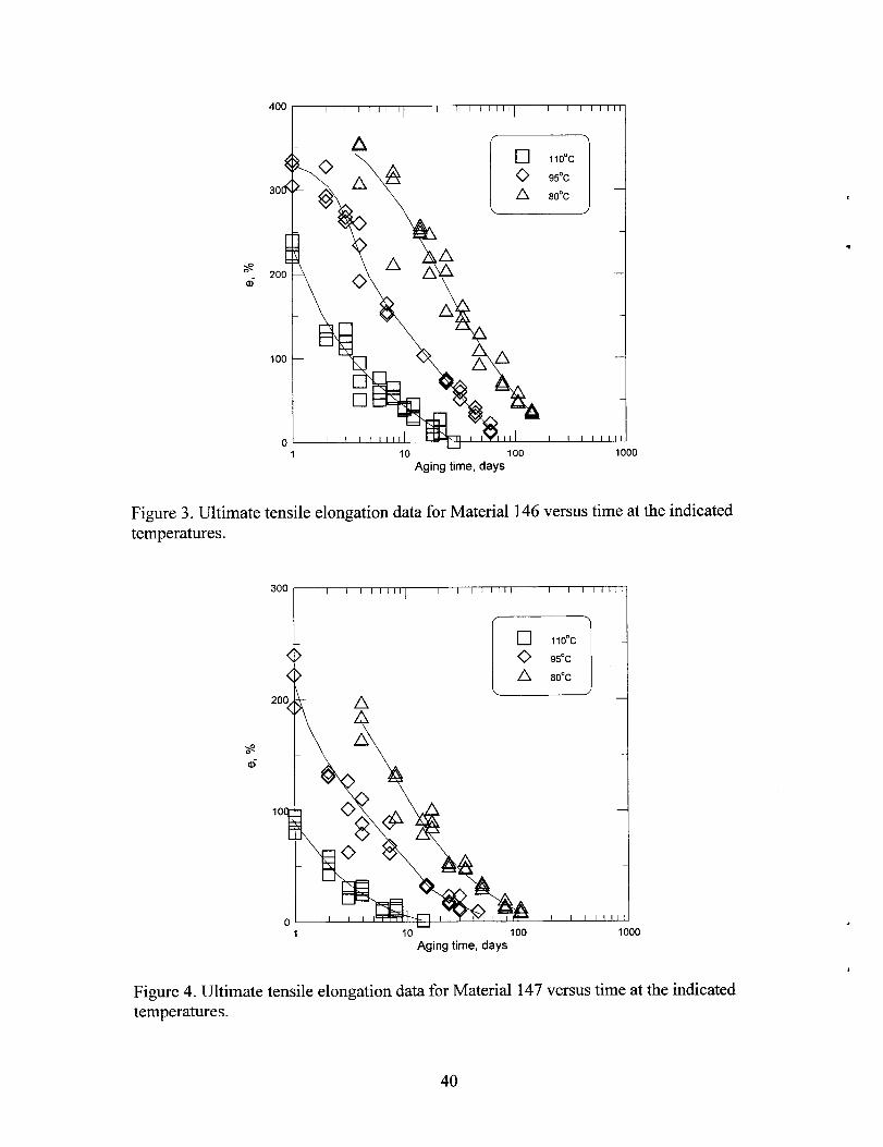
sa)-
400 I I I I I I 11] I I I I I I Ill I I I I I Ill
I
IkllA200 0 ‘A
A
El•1 11O”C
o 95°c
~ 80”C
“
1 10u 100 1000
Aging time, days
Figure 3. Ultimate tensile elongation data for Material 146 versus time at the indicatedtemperatures.
300 I I I I I I Ill I I I I I Ill I I I I I 111
I
El•1 Ilo”c -0 95°C
~ 80°C
—
Aging time, days
Figure 4. Ultimate tensile elongation data for Material 147 versus time at the indicatedtemperatures.
40
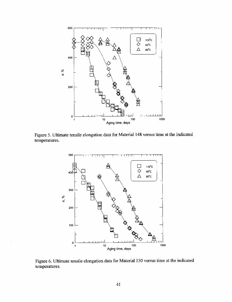
600
{(
(
400
~
11-
200
0
I [ I I I 111[ I I I I I I II I I I I I I
gw L-.--)•1 Ilo”c
80 0 95°C
-1%
~ 80”C
Ao
1 10 100 1000Aging time, days
Figure 5. Ultimate tensile elongation data for Material 148 versus time at the indicatedtemperatures.
500 I I I I I I II I I I I I Ill] I I I I I I II
, \
300
200
100
I
PI
ol I I I 1 1 I Ill 1 I I i I I Illv
I I h-’! I !11
1 10 100 1000Aging time, days
Figure 6. Ultimate tensile elongation data for Material 150 versus time at the indicatedtemperatures.
41
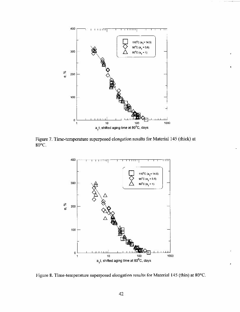
400 I I I I I 1111 I I I I I I Ill [ I 1 I I I II
300
200I
\
8
1IO”C (aT= 14.5)
95°C (aT=3.6)
~ 80°C(aT=l) I100 —
o I I 1 I I 1 II I I I I I I I I ! I 1 1[
1
Figure 7. Time-temperature
80°C.
10 100 - 1000
a~t, shiiled aging time at 80°C, days
superposed elongation results for Material 145 (thick) at
400 I I I I I I II I I I I I I Ill I I I [ I I I I
ga.-
200
t
100In!g110”C (a~=14.5)
95°C (aT=3.5)
~ 80°C(a,=1)
A
1b, I I I I ILo~
1 10 100 — 1,,
1000
a+, shifted aging time at 80°C, days
Figure 8. Time-temperature superposed elongation results for Material 145 (thin) at 80”C.
42

300 —
200 —
100 —
o—1
A
L_____l\
81Io”c (aT=15)
95°C (a~=3.6)
+@~ 80°C(aT=l)
AA
#
•1
I I I I I I Ill I I I I I I II 1 I 1 Ill
10 100 1000
a~t,shifted aging time at 80°C, days
Figure 9. Time-temperature superposed elongation results for Material 146 at 80°C.
300 I I I I I I 11] I I I I I I Ill 1 I I I I [11
100
0
A
o
I I I I I I II I I I I I I [ I I I I II
1 10
u100 1000
a~t, shifted aging time at 80°C, days
Figure 10. Time-temperature superposed elongation results for Material 147 at 80”C.
43
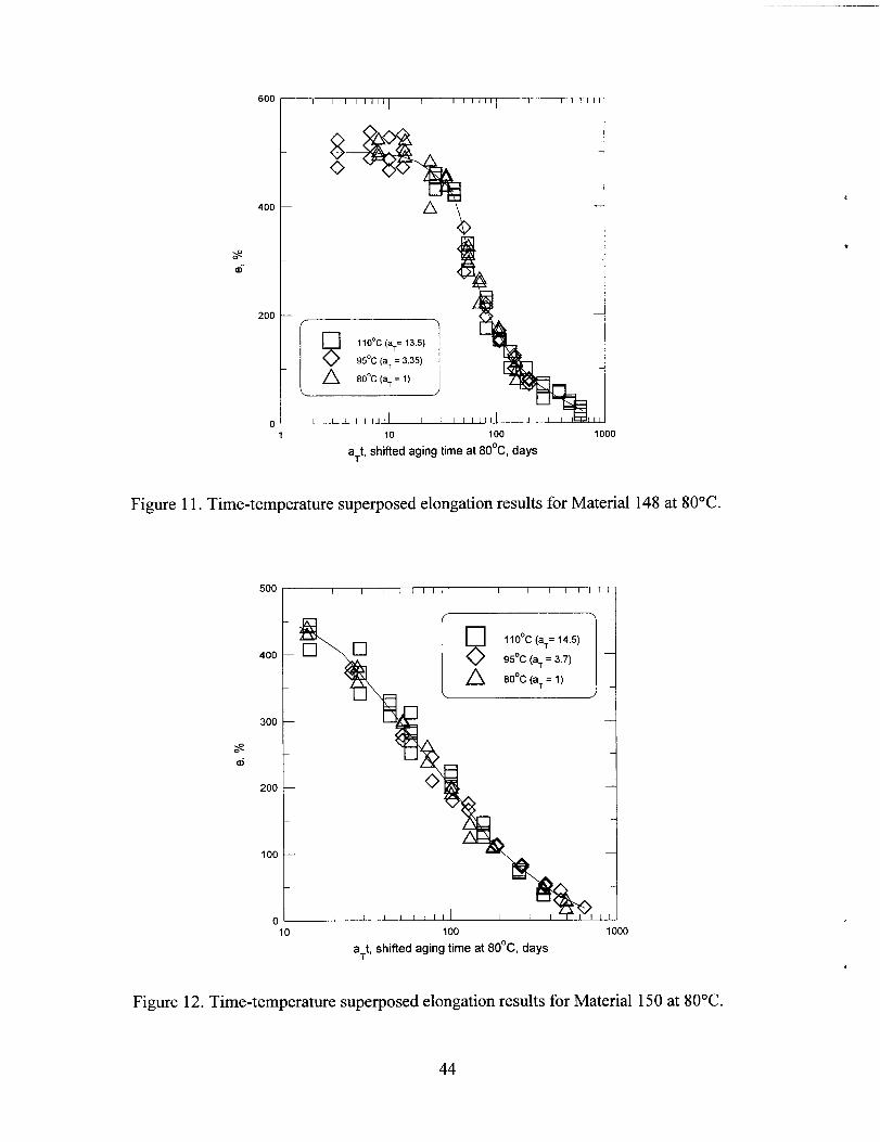
600
400
<.a)-
200
I I I I I I 11/ I I I I I I Ill I I I I I I
4[El811O°C(aT=13.5)
95°C(aT = 3.35)
~ 80°C(.T= 1)
01 1 I I I I 1111 I 1 I I I 1111 I I I t I1 10 100 1000
aTt, shifted aging time at 80°C, days
Figure 11. Time-temperature superposed elongation results for Material 148 at 80°C.
500
400
300
~
a)-
200
100
0
I I I I [ I I I I I I I I 1 I I
Ii
I
—
1 I I I I I I I I I I 1 I
-lo 100 1000
a~t, shifted aging time at 80°C, days
Figure 12. Time-temperature superposed elongation results for Material 150 at 80°C.
44

1.2 I 1 8 I 1 I II I ! 1 I 1 1 II 1 1 1 I I 1 II
1.0 —
0.8 —
0.6 —
0.4—
0.2— a-’•1
0.0 I I I I I [111 I [ 1 I I I [11 I I 1 I I I II
1 10 100 1000
a+, shifted aging time at 80°C, days
Figure 13. Superposition of tensile strength values for Material 145 (thick)values from the elongation superposition.
1.2
1.0r
1 Ill I I I I 1 I II 1 I 1 1 1 (
8
110”C (aT= 14.5)
95°C (aT= 3.5)
~ 80”C(a,= 1)
0.8
Ha o
- .-1 10 100 1000
a+, shifled aging time at 80°C, days
Figure 14. Superposition of tensile strength values for Material 145 (thin) using aT valuesfrom the elongation superposition.
45

I ,-- 1
8
110”C(aT=15)
95°C(aT=36)
~ 80”C(a,=1) {
1
o.o~1 10 100 1000
a+, shifted aging time at 80°C, days
Figure 15. Superposition of tensile strength values for Material 146 using aT values fromthe elongation superposition.
1.2 1 I I 1 I 1 II I I I I I I 1+ I ! I 1 I 1 II
t1.0 1-
0.2
I
,-----J8110”C (aT= 15)
o 95°C(aT= 3.15)
8
A So”c(a,= 1)
A
“R
❑
•1El
t i
1 10 100
a+, shifted aging time at 80°C, days
Figure 16. Superposition of tensile strength values for Materialthe elongation superposition.
1000
147 usingaT dues from
46

1.2, 1 I [ I 1 IA1 I A I 1 I I I 1 11[ 1 1 1 I I 1 Ill
1t—————— 1
0,0~
1 10 100 1000
a+, shiftad aging time at 80°C, days
Figure 17. Superposition of tensile strength values for Material 148 using aT values fromthe elongation superposition.
1.2 1 1 I 1 I 1 Ill 1 1 I 1 I 1 II [ I 1 1 I 1 II
1.0:1
0.8
0.6—
0.4—
0.2 —
o00
0,0~
10 100 1000
a+, shifted aging time at 80°C, days
Figure 18. Superposition of tensile strength values for Material 150 using aT values fromthe elongation superposition.
47
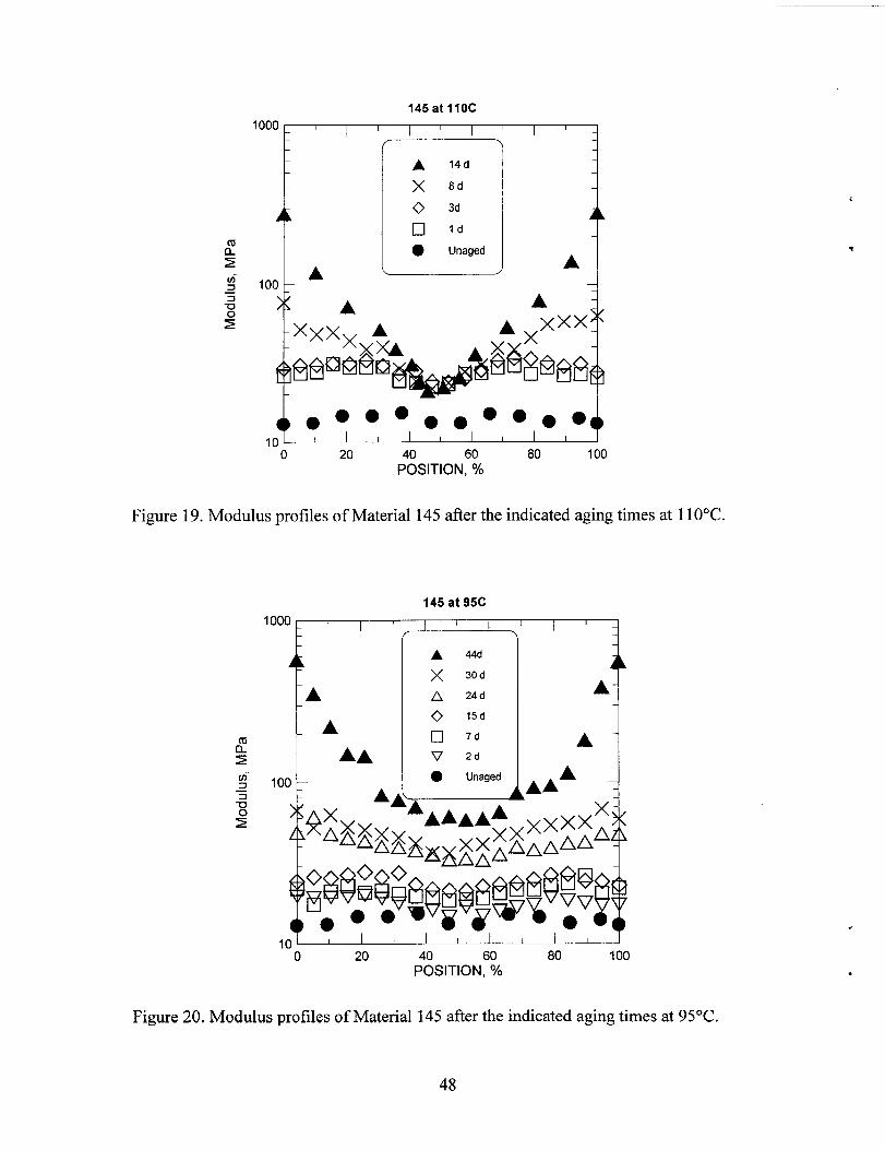
145at IIOC
1000 ~ 1 I 1I
1I
1I
!4
I
A 14 d
)( 8d
O 3d
❑ Id
● Unaged
-4
1A . .
.000oo@ogo10 ! I I I 1 I 1 1 I
o 20 40 60 80 100POSITION, %
Figure 19. Modulus profiles of Material 145 after the indicated aging times at 11O“C.
145at 95C
‘OOO~
t
A 44d
x 30d
A A 24 d A f
10I I I I I I I 1 I 1 I
o 20 40 60 80 100POSITION, %
Figure 20. Modulus profiles ofMaterial 145 afterthe indicated agingtimesat95°C.
48
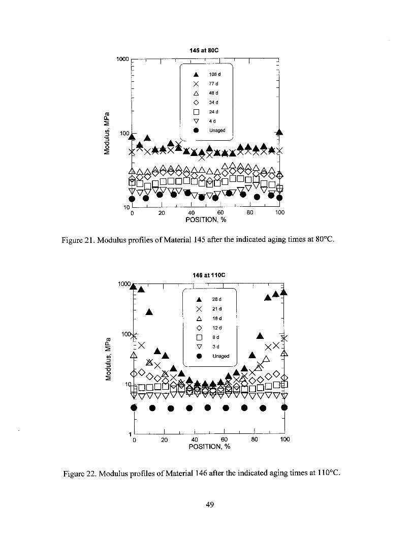
145 at 80C
#%#w&i&#$%3j?:Vg?wiillwv=vgww●v&
10 1 I 1 I I I I
o 20 40 60 80 100POSITION, %
Figure 21. Modulus profiles of Material 145 after the indicated aging times at 80°C.
146atl10C
1000A’
I I I I I I I
A 28 d#
i
Ax 21d
A 18d
Q 12d
10 ❑ 8d A i
?
● 000000 !,~
o 20 40 60 80 100POSITION, ~0
Figure 22. Modulus profiles of Material 146 after the indicated aging times at 11O“C.
49

146 at 95C
1000_ I I I 1 [ If
I I> I
A 60d
x 44d
A 32d
o 24d
100 T❑ 15 d
v 4d
i
HAA.AA‘AAAAAAAAAAAAX XX I‘ iiiiiiiii$$$$izi$fxi
● ae *e**?
t 1,~
o 20 40 60 80 100POSITION, %
Figure 23. Modulus profiles of Material 146 after the indicated aging times at 95”C.
146 at 95C
t 1,~
o 20 40 60 80 100POSITION, ~0
Figure 24. Modulus profiles of Material 146 after the indicated aging times at 80”C.
50
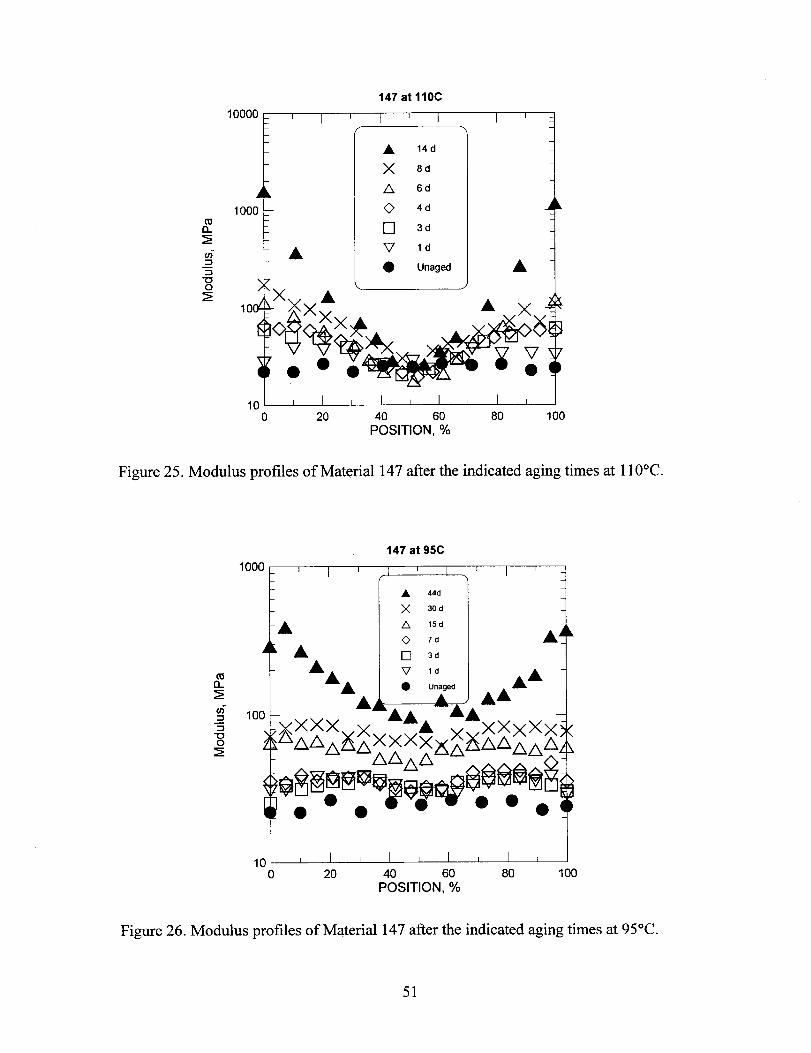
147at IIOC
10000 L I I I I I I I I I -1
1000L n1 I I
A 14 d
)( 8d
A 6d
o 4d
❑ 3d
v Id
● Unaged A-5 A————__Jz
$s’d; ~10 I I I I I I I !
o 20 40 60 80 100POSITION, %
Figure 25. Modulus profiles of Material 147 after the indicated aging times at 110”C.
147 at 95C
‘OOO ~
ii
A
l---’%,A 15d
0 ?d AA ❑ 3d
‘AA : :;,,,, AA
A AAAA A’00Xxxx x A x XxXxX
‘AAAZAX XXXXA~AAAAA
Gf3E:~Q$~@*$@$@@8● 0°
● 00
,0 ~
o 20 40 60 80 100POSITION, %
Figure 26. Modulus profiles of Material 147 after the indicated aging times at 95°C.
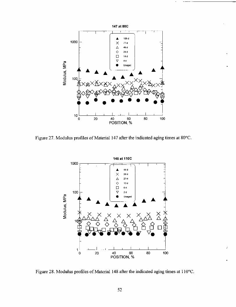
147at 80C
I I I II
[ I I
f’I
\I
,(-J ~
o 20 40 60 80 100POSITION, %
Figure 27. Modulus profiles of Material 147 after the indicated aging times at 80”C.
148 at IIOC1000 _ I I
/- I,-)
I I
A 44d
x 28d
A 20d
O 10d
❑ 6d
100 : v 2d
,~o 20 40 60 80 100
POSITION, ~0
.
.
;
a
Figure 28. Modulus profiles of Material 148 after the indicated aging times at 11O“C.
52
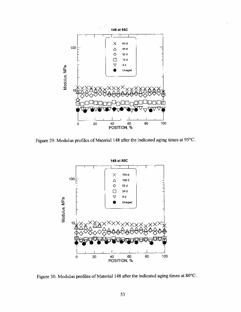
148 at 95C
I I 1 I I I If
I -1 I
x 60d
100 – A 44d
O 32d
❑ 15d
v 4d
● Unaged
L /
1 I I I 1 I I I I
o 20 40 60 80 100POSITION, ~0
Figure 29. Modulus profiles of Material 148 after the indicated aging times at 95”C.
148 at 80C
, 1 1 1 I I I II
)x 154d ~
A 106 d
O 55d
❑ 24d
v 8d
● Unaged
i
1
I I I I I 1 I I
o 20 40 60 80 100POSITION, %
Figure 30. Modulus profiles of Material 148 after the indicated aging times at 80°C.
53
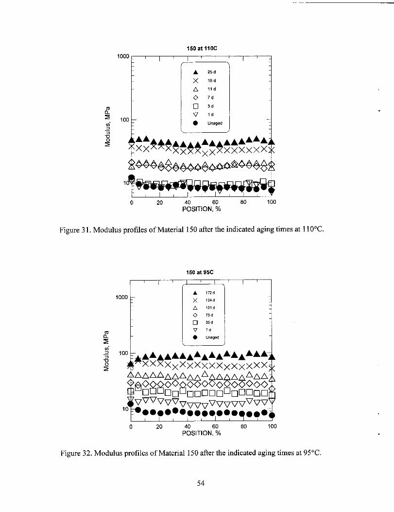
150atl10C
1000 _ I I I I 1 I I I [
jn;
A 25d
x 18d
A Ild
O 7d
❑ 3d
CTz
v Id100
ul- ● Unaged3
5m
2 AA AAAAAAR****$**XX*XXXXXX
[ I I 1 I I I I I 1 Y
o 20 40 60 80 100POSITION, %
Figure 31. Modulus profiles of Material 150 after the indicated aging times at 11O“C.
150 at 95C
I I I I I [ I/ I \ I
1000
1’z.1 l-----J
A 172d
x 124d
A 101d
o 73 d
❑ 35d
v 7d
● Unaged
w=7 A AAAAAAAAAAAAAA7J
*XAXXXXXXXXXXXXXXsAAAAAAAAAA A AAAAA
%8g&&#&%zzElT7m7m7~~~.@7vv@7vT7
10 ●0oooooo.OOOoq..oI i 1 1 I
o 20 40 60 80 100POSITION, %
,
d
Figure 32. Modulus profiles ofMaterial 150 afiertheindicated agingtimesat95°C.
54

150 at 80C
1000 1 I I I I I I(
I \ I
A 495 d
x 363 d
A 182d
o 132 d
❑ 73d
v 14 d
● Unaged
100 – \ J
A ~~AAAAUAAAA~A/@ J
04000000000000000< )‘nnOn[lnnrlananOUDDuE ]1 Vwgmvwvwuvvvuq
10 20 40 60 80 100
POSITION, %
Figure 33. Modulus profiles of Material 150 after the indicated aging times at 80”C.
400
c-0 300.-xUY~ala~ 200al>m
t
El❑ llo”c
o 95°C
A 80°C
•1
‘O:L10 100 1000
Surface Modulus, MPa
Figure 34. Elongation versus surface modulus for Material 145 (thick).
55
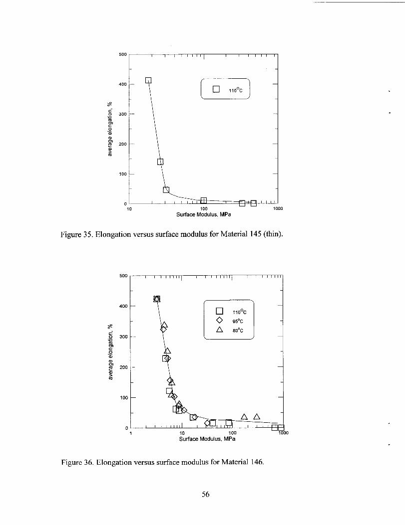
500
400
&oc-0 300.—zml
~ma)u)m 200G>m
100
0
I I I 1 I I I 1 I I I I I I I I
\
m
\\\
I I I I I I I tll 1 I I I
10 100u
i 000
Surface Modulus, MPa
Figure 35. Elongation versus surface modulus for Material 145 (thin).
500 I I I I I I II I I I I I I II I I I I I I II
I
o I I I I I I II I, ,,
El❑ Ilo”c
o 95°C
~ 80°C
1 10 100 -WooSurface Modulus, MPa
Figure 36. Elongation versus surface modulus for Material 146.
56
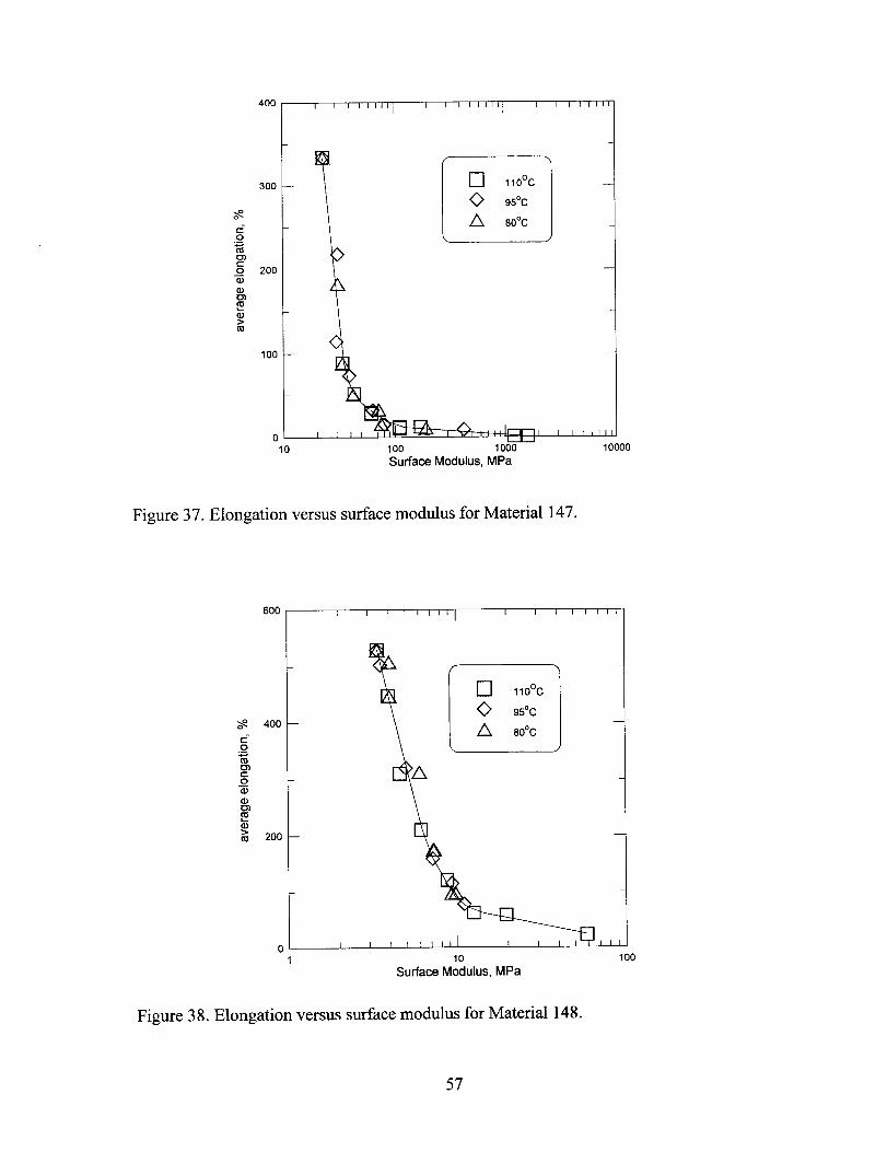
400 I I I I [ I II I I I I I I II I I I I I I II
300 —
\ r
•1 11O”C
o 95°c~
~ 80°Cc-0.—xi01~
3200 —
a)almmk>m
100 —
o~ I I I I I 1 IA Im , I I I I I II
10 100 1000 10000
Surface Modulus, MPa
Figure 37. Elongation versus surface modulus for Material 147.
600 I I I I I I I I I I I I I I I I
~ 400 —
c-0.-%0~a)a)mm%>m 200 —
0 I I I I I I 1 I I I I I
1 10 100
Figure 38.
Surface Modulus, MPa
Elongation versus surface modulus for Material 148.
57

almm&>l-u
500, 1 I 1 I I 1 1 1 I 1 I 1 1 1 1 I
400 —
300 —
200 —
100 —
o
•1 11O”C
o 95°c
A 80°C
a’
•1\❑ ✼
,Il,,l,,lhA
o
1 100
Surface M~dulus, MPa
Figure 39. Elongation versus surface modulus for Material 150.
ualN.—
%
E5z
I I I I
0 +!!l0
A
0.
..L•1 Ilo”c
o 95°C
A 80°C
I 1---
.
0 100 200 300 400
elongation, ‘h
Figure 40. Elongation versus normalized tensile strength for Material 147.
58

I I I
3:❑ 96.5°C
o 65°c
I
,.-11~o 400 800 1200 1600
Aging time, hours
Figure 41. Oxygen consumption rate results for Material 145.
10-”0
II
[I
I I-1
l-l
❑l-l ❑ 96.5°C
O 65°C
I I I I
400 800
Aging time, hours1200 1600
Figure 42. Oxygen consumption rate results for Material 146.

t
n❑ 80”C
O 65°C
,011L——L4—Jo 200 400 600 800 1000
Aging time, hours
Figure 43. Oxygen consumption rate results for Material 147.
10-”0
I I I 1 I
I I I I I I200 400 600 800 1000
Aging time, hours
Figure 44. Oxygen consumption rate results for Material 148.
60
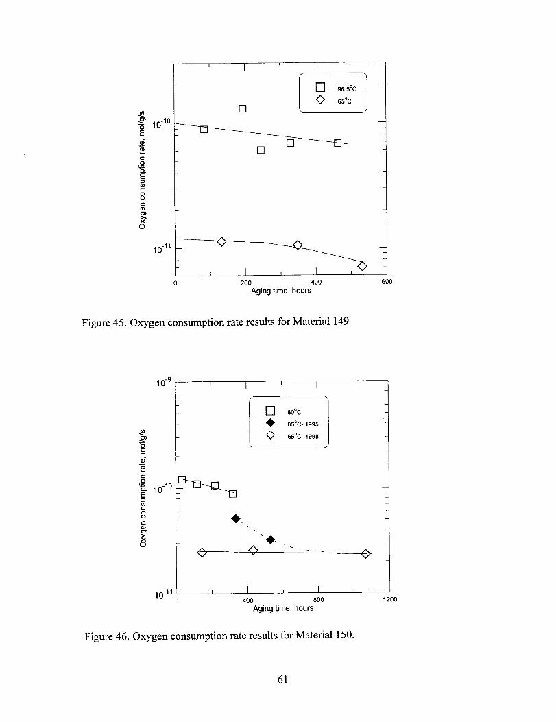
I I I i
El_❑ 96.5°C
O 65°C
(n ❑h~ 10-’0 ~EJIJ- ❑m ❑co.-3 t
o 200 400 600
Aging time, hours
Figure 45. Oxygen consumption rate results for Material 149.
10-9
a)-5c0
“~10-’0smcoc1
10-”
I I I
E❑ 80°C
+ 65°C-1995
0 65°C-1998
q
‘+- . ..-
V
I I I I
0 400 800 1200
Aging time, hours
Figure 46. Oxygen consumption rate results for Material 150.
61
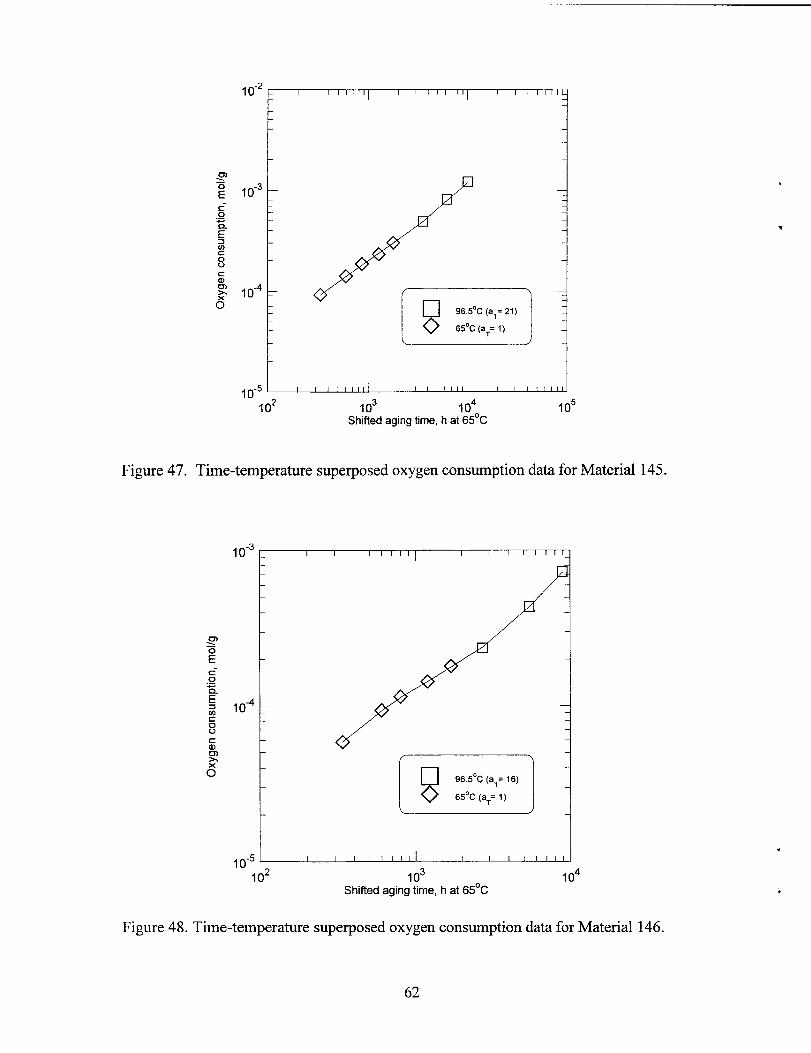
0)>
E
10“2- I I I 1 I [ Ill I I I 1 I 1 II [ I 1 1 I 1 IL
10-3
,0-4
I
t 1,.-5~
102 103 104 105Shifted aging time, hat 65°C
Figure 47. Time-temperaWre supe~osed oxygen consuption data for Material l45.
I
E,“
102 103 104Shifted aging time, hat 65°C
Figure 48. Time-temperature superposed oxygen consumption data for Material 146.
62
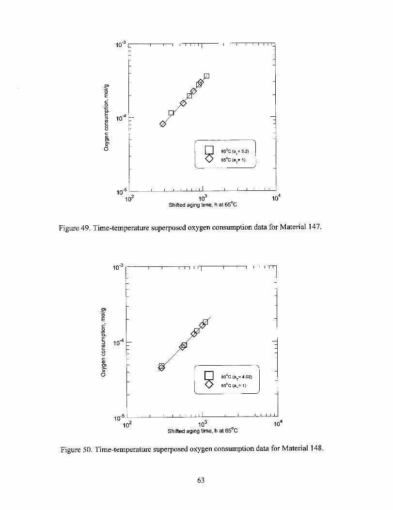
c-0.-IiE3Inc00
104-/
E!,..5 I I I 1 I I ! I I I I I I I I I
102 103 104Shifted aging time, hat 65°C
Figure 49. Time-temperature superposed oxygen consumption data for Material 147.
I I I I I I I I I I I I I I I 1
,.-5~
102 103 104Shifted aging time, hat 65°C
Figure 50. Time-temperature superposed oxygen consumption data for Material 148.
63
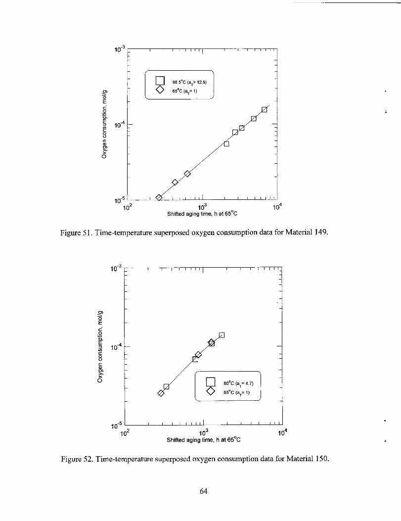
c-0.-ZE3UYc0cl
10-4:
, ‘-5 [ [ I
102 103 104Shifted aging time, hat 65°C
Figure 51. Time-temperature superposed oxygen consumption data for Material 149.
10-3_ I I I I I I I I [ I I I I I I I
>g
E
s-0.—zE~ 104co0ca)m
E
:/;E
10-5
102 103 104Shifted aging time, hat 65°C
Figure 52. Time-temperature superposed oxygen consumption data for Material 150.
64
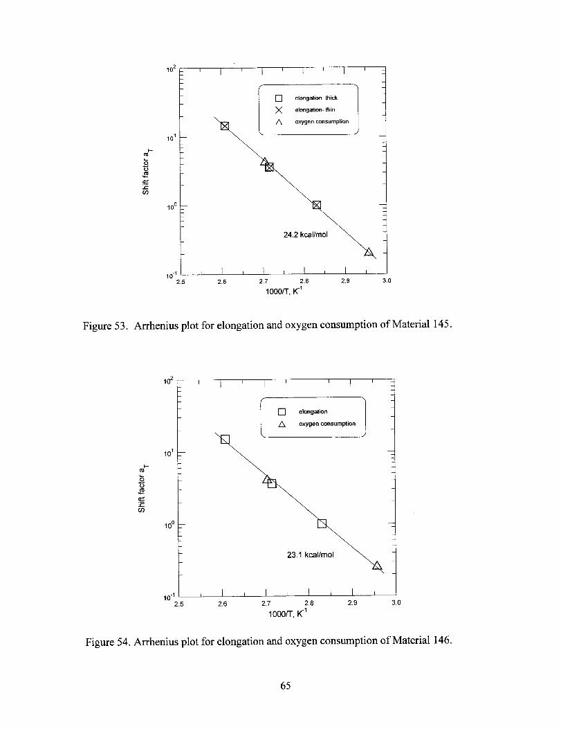
!5sCn
102 – I 1 I I I
10’
10° z
24.2kcalimol
,.-1 ~
2.5 2.6 2.7 2.8 2.9 3.0
1000i-r,K’
Figure 53. Anhenius plot forelongation adoxygen cons~ption of Material l45.
I ❑ elongation
A oxygen consumption
‘f%
\
I I,.-1 ~
2.5 2.6 2.7 2.8 2.9
1000rl-,K’
3.0
Figure 54. Arrhenius plot for elongation and oxygen consumption of Material 146.
65

P-m
102 – I I I I I
10’
10° :
24.2kcallmol
,.-1 ~
2.5 2.6 2.7 2.8 2.9 30
1000/T,K’
Figure 55. Arrhenius plot for elongation and oxygen consumption of Material 147.
1-(Q
10’
10° r
23.0kcal/mol
,.-7 ~
2.5 2.6 2.7 2,8 2.9 3.0
1000/T, K-’
Figure 56. Arrhenius plot for elongation and oxygen consumption of Material 148.
66
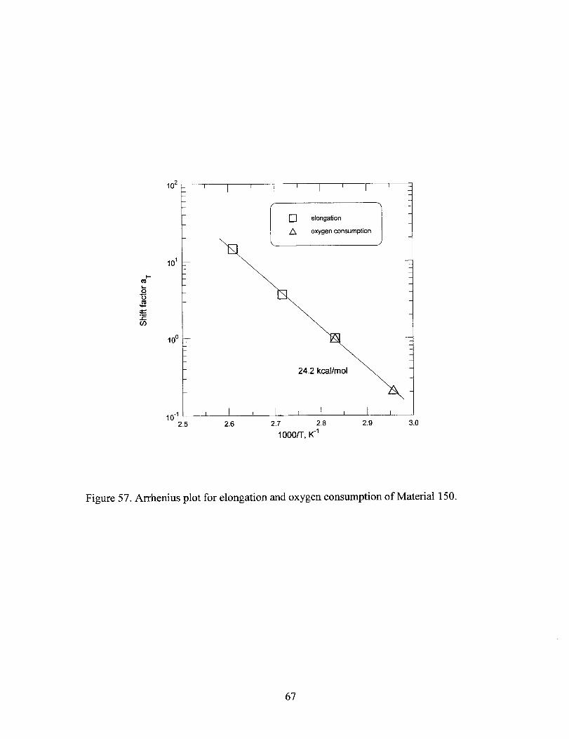
1-m
102 - I I I I 1
10’ z
10° z--
24.2 kcal/mol
,.-4 ~
2.5 2.6 2.7 2.8 2.9 3.0
1000/1.K-’
Figure 57. Arrhenius plot for elongation and oxygen consumption of Material 150.
67

P= O.1,ci as shown p =5, iI as shown1.0
0,8
co
“: 0.6.-
$a)>.—Z 0.4
2
0.2
0.0 ,0 20 40 60 80 100
1.(J
0.8–
0.6–
0.4–
0.2 –
0.0 Io 20 40 60 80 100
P, % P, 70
p = 100, u as shown p = 1000, cc as shown1.0
0.8–
co
co
~“ 0.6—.-3
.— -0.-$ 8~ al.— >~ 0.4–
.—~
1!? c?
0.2–
0.0 I I !0 20 40 60 80 100
P, %
1.0 ly-
0.8–
0.6–
0.4–
0.2–
0.0 I I \( I )0 20 40 60 80 100
P, ‘?40
40K
I !
Figure 58. Theoretical relative oxidation profiles for planar material surrounded byoxygen on both sides as a fimction of various combinations of the diffision-limitedoxidation parameters a and P.
68


Figure 61. Photograph of modified oxygen permeability apparatus.
I
❑
0xA
v●
■
f?
+
%
100%
60%
50%
40%
30%
21%
10.5”,6
5“/6
1%
,.-10 ~
2.40 2.80 3.20 3.60
1000/T,K-’
*
Figure 62. Temperature-dependent oxygen permeability results versus oxygen partialpressure without corrections for reaction.
70
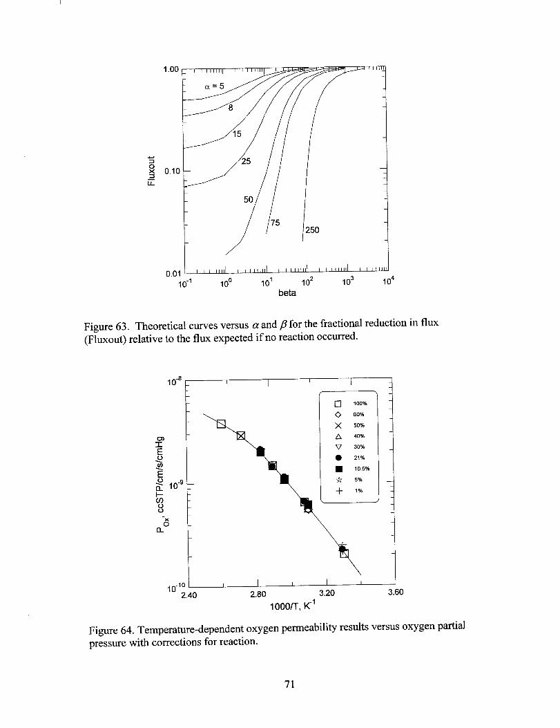
‘“”Wt /’//11 1
0.01 I I 111 [11 [ I I 1! 111 I I I 1 [1111 ! I I 111111 I ! I Ill
10-’ 10° 10’ 102 103 104
beta
Figure 63. Theoretical curves versus a and/? for the fractional reduction in flux(Fluxout) relative to the flux expected if no reaction occurred.
10-8_ I I I
qJ ‘:
❑ 100%
O 60%
x 50%
A 40%
~ v 30%
o ● 21%
2
z■ 105%
* 5%
; 10-9:1-
+ 1%
~
c-)
-xoCL
10-’0‘ I I I I I I
2.40 2.80 3.20 3.60
1000/1, K-’
Figure 64. Temperature-dependent oxygen permeability results versus oxygen partialpressure with corrections for reaction.
71
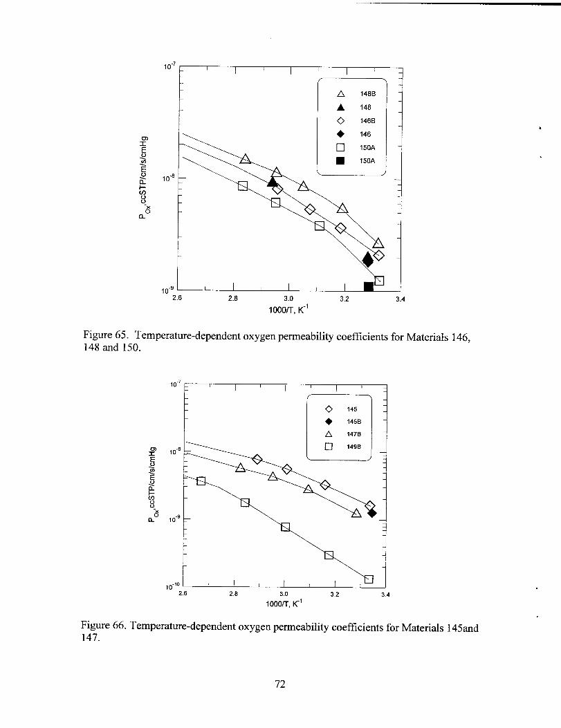
I I I I
n:
A 1480
A 148
0 1460
+ 146
\\ .❑ 150A
\
—
“’-’$
~hj6
■h<n-g I I I
‘“ 2.6 2.8 3.0
1000/T, K-’
Figure 65. Temperature-dependent oxygen permeability148 and 150.
3.2 3.4
coefficients for Materials 146,
10-’L 1 I 1 I I I I i
10-8
10“9
710 145
+ 145B
A 147B
,O.lOF,,, ,>~2.6 2.8 3.0 3.2 3.4
1000/1, K’
Figure 66. Temperature-dependent oxygen permeability coefficients for Materials 145and147.
72
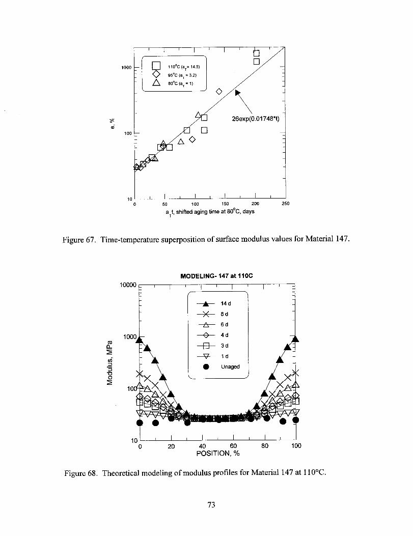
1I
I I II
I
Cl
8
•1
1000 11 O“c (aT=14.5)
95°C(aT= 3.2)
~ 80°C(aT=l)
o
26exp(0.01748*t)
100
<
,o~o 50 100 150 200 250
a~t, shifted aging time at 80°C, days
Figure 67. Time-temperature supe~osition ofsufiace modulus values for Matetiall47.
MODELING- 147 at IIOC10000~ I I 1 I I I I I 1
3
141000
+ 14d
+ 8d
-z2r- 6d
--+- 4d
+ 3d
+ Id
● Unaged
10
,o~o 20 40 60 80 100
POSITION, ~0
Figure 68. Theoretical modeling of modulus profiles for Material 147 at 11O°C.
73
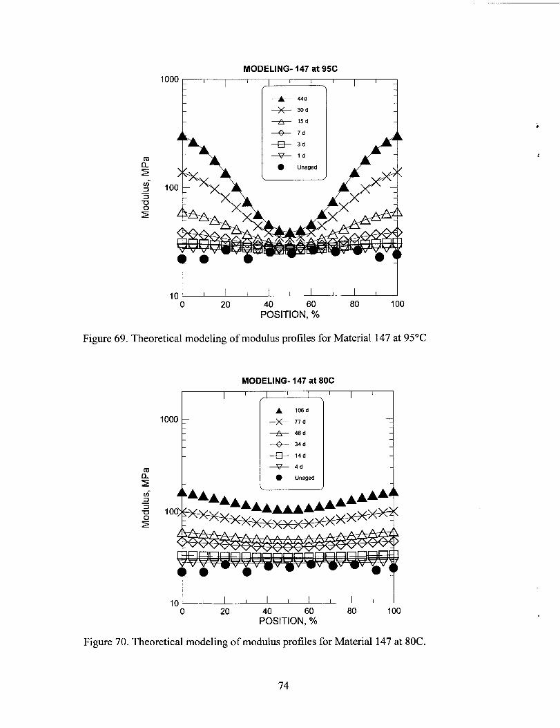
MODELING- 147 at 95C1
OOOr’E=r7ti
+- 7d.A
++ 3d
+ Id
● Unaged /- \
K T
,’~0 20 40 60 80 100
POSITION, ~0
Figure 69. Theoretical modeling of modulus profiles for Material 147 at 95°C
MODELING- 147 at 80C
I I I I(’
I I1
A 106d
+ 77d
+ 48d
+ 34d
+ 14d
-W- 4~
● Unaged
10
,’ ~
o 20 40 60 80 100POSITION, %
Figure 70. Theoretical modeling of modulus profiles for Material 147 at 80C.
74

10000 I I I I
. D = 2.48e% cm2/s. . . S = 1.39e-3 ccSTP/cc/cmHgP = 3.45e-9
m: 1000— ‘~’..,,,‘=-
•~’..,,,n
. . . . . . .
100 I I I I
o 10 20 30 40
L214t, 10-5
Figure 71. Plot of log[F(t05)] versus 12/(4t) for EPDM material.
10000
1000
IL+0-
100
10
I I I I I
..
‘El.n.
.
‘D.,, a
..
I I I I I
o 5 10 15 20 25
L2)4t, 10-5
Figure 72. Plot of log[F(t0”5)] versus 12/(4~)for Material 147.
75
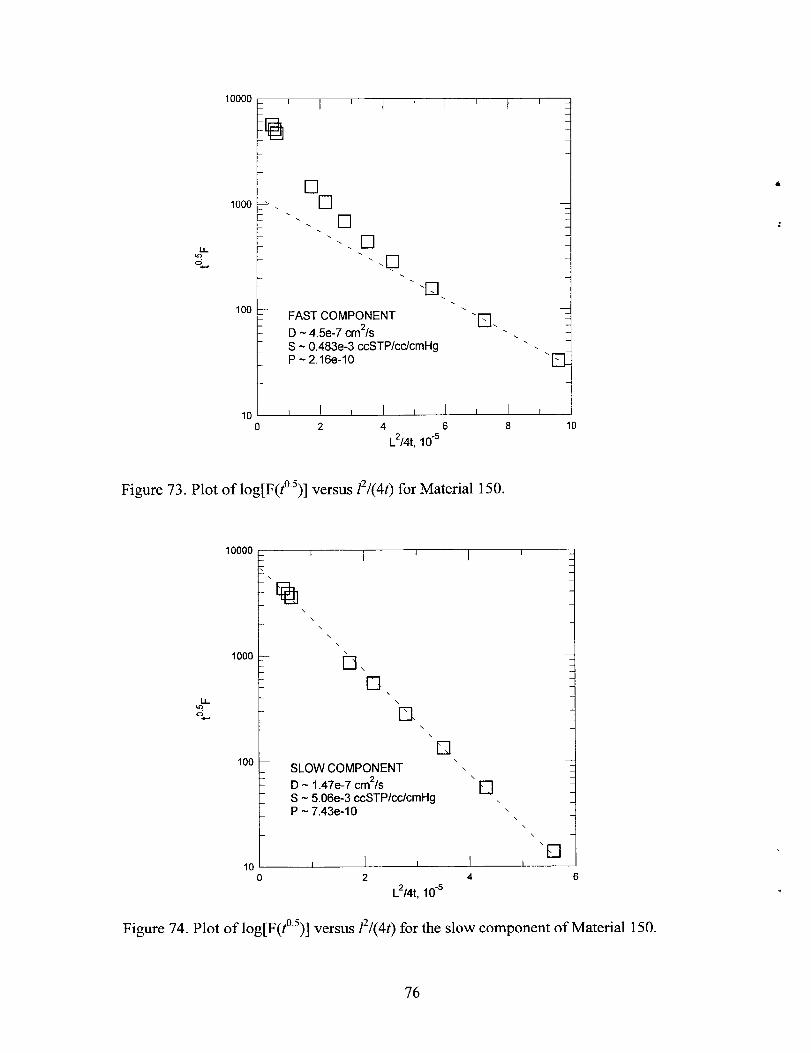
‘OOOO~
#%
piia1000 +
100 :
In 1-
❑❑
. . ,0.‘.CI.
‘.0.
“Q 1. .FAST COMPONENT
D - 4.5e-7 cm2/sS - 0.483e-3 ccSTP/cc/cmHgP-2.16e-10
I I I I I.“
o 2 4 6 8 10
L2/4t, 10-5
Figure 73. Plot of log[F(t05)] versus 12/(4t) for Material 150.
10000 I I I
\\ :
1000 =
100 :
\\
\\
\
b. 4El I
SLOW COMPONENT ‘ \D - 1.47e-7 cm21sS - 5.06e-3 ccSTP/cc/cmHg
‘a\
P - 7.43e-10 \\ 1
‘ElII-I I I I I.-
0 2 4 6
L214t, 10-5
Figure 74. Plot of log[F(t05)] versus 12/(4t) for the slow component of Material 150.

loo~ ,, , ,1 I I I -1
10 –
I
1 I ,
1
1● unaged , 1 1
I , — expected I, 1 1
1 , I
I , I
\ 1
1
1 t
I ,
I
I
1 p- o-a
1
1 *-‘0
●Oe. -
I
J :I
I
149 : 146 : 145 ~ 148 150
1 I , , I I I , I
o 20 40 60 80 100P, %
Figure 75. Modulus profiles for laminate material and expected resultsmaterial properties.
1.0
0.8
0.6
0.4
0.2
I ( I I I I I
,\ /
\’ /
\’( ,
/
\’1 I /
1’I I I /
1’1,
1’
!
~ /
,,
,’1,
1’1)
1’,/
,’If
1’,/
1’,/
,!
\,/
,\{
1$ !,
l\ j,
Ill {l
/
I\l
[ ~ “.:
/
‘/(
I/
0.00
/,I
20 40 60 80 100
based on isolated
P, %
Figure 76. Modeling results for laminate using parameters from Table 9. Solid curvegives oxygen concentration profile whereas dashed curve gives oxidation profile.
77

100-40 40-11 11-1.2-13 13-37 37-1ooloop ,, , ,, I I 1I I 4
t“I
~ H 28dat95°C
(
1
, 1
1‘* Unaged
F I
149 146 ‘ 145 ‘ 148 ‘ 150 I
11 I I I I I I
o 20 40 60 80 100P, Yo
Figure 77. Experimental modulus profiles for aged and unaged laminates.
LARGE TIRE SIMULATION- 10OC
2.5 ,, I I I I I I II(1,1 I
— Relativeoxygenconcentration
.—
5_’?#
,
0.=
g
0w
~
0.0 1,
0 20 40 60 80 100P, Yo
Figure 78. Large tire simulation at 100”C using the input parameters given in Table 10.
78

SMALL TIRE SIMULATION- 70C
1.61 ,, ,, , ,, I I I I
r\,\1.2 ‘, ‘,(!’\’{,.
0.8 :
0.4 :
,$ I
I
{ I (
, . ‘/I I
‘ /.\ /,, (/
,\\’ ,, ‘
,., /, /., ., .,/
.,./
-~110.0
0 20 40 60 80 100P, %
Figure 79. Small tire simulation at 70”C using the input parameters given in Table 11.
7
6
5
4
3
2
1
0
u.,, ‘—+— New;:
;ti,:
cl:. -.. . - Lab-Tested,,., I,, I,,,,.’ i
IJ
t
I
I
o 10 20 30 40 50 60 70 80 90 100
Relative Position
Figure 80. Oxygen content (wt. Yo)for lab-tested tire and new tire.

3.5
3
2.5
2
1.5
1
0.5
0
-0.5
0 10 20 30 40 50 60 70 80 90 100
Relative Position
Figure 81. Change in oxygen content in lab-tested tire.
Figure 82.
I
5 I o ——t—New,,I ,, I
-0--- In-service
I
3 ; ‘b [
2. ❑ .._- ----- -
1
0.I
o 10 20 30 4(3 50 60 70 ~. go 100
RelativePosition
Oxygen content (wt. ‘%0) for in-service tire and new tire.
.
80
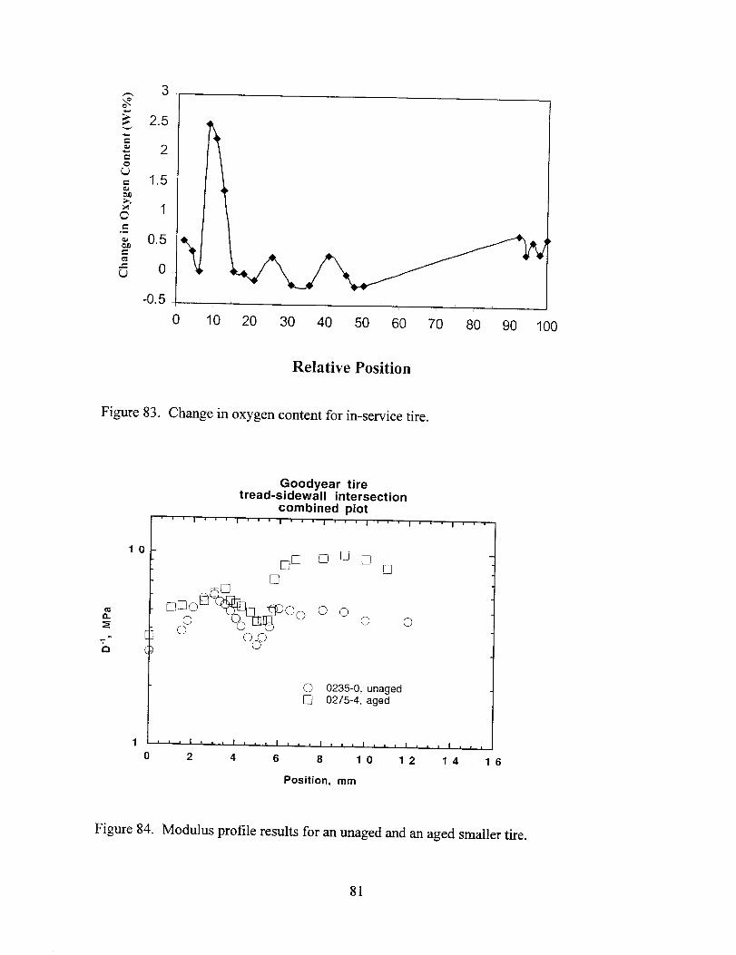
o 10 20 30 40 50 60 70 80 90 100
Relative Position
Figure 83. Change in oxygen content for in-service tire.
Goodyear tiretread-sidewall intersection
combined plotI I I I I I I
10 ❑nnnn
•1❑
❑uo %Qa
u@
❑ O.OOO
0° 00 00.O
(J
O 0235-0, unaged❑ 0275-4, aged
1 I I I I I I I
o 2 4 6 8 10 12 14 16
Position, mm
Figure 84. Modulus profile results for an unaged and an aged smaller tire.
81

Goodyear tirecross-section of sidewall
1 02 I II r
O unaged
❑ aged
[1
1@ @oC9U
(-’-l
•1 “cl
@00 1,!
❑o&g[1
(3
1 0° 1 I ,
0 50 100
P, %
inside interior outsidelayer components layer
insideedge
Figure 85. Modulus profile results formunaged mdmaged tire sidewall.
82

1 02
1 o’
1 0°
1’ I I I d
@-p+o0
Iedge of tread
aged tire22.95mm
o
0 unaged1
o
\edge of tread
unaged tire38.00mm
/L I 1 I 1
0 10 20
Position, mm
30
Figure 86. Unaged and aged modulus profile results for a larger size tire.
12
I10
t
L-----2 0 2
POSITION, mm
4
40
Figure 87. Modulus profile of two samples (134-2) with tread surfaces touching at Omm.

up eX——— ——. ._
-. —-. . - -_ _
.~ --
—. —-— --
Figure 88. Sketch of the cross-section of the apex region of tire ER-1 001.
t
I
“’[m
A -i
t——————’ -1
II I I I I I I
o 20 40 60 80 100Position, !40
●
✞
Figure 89. Modulus profiIes ofapexregion ofunaged mdagedsmples of ER-l OOl.
84
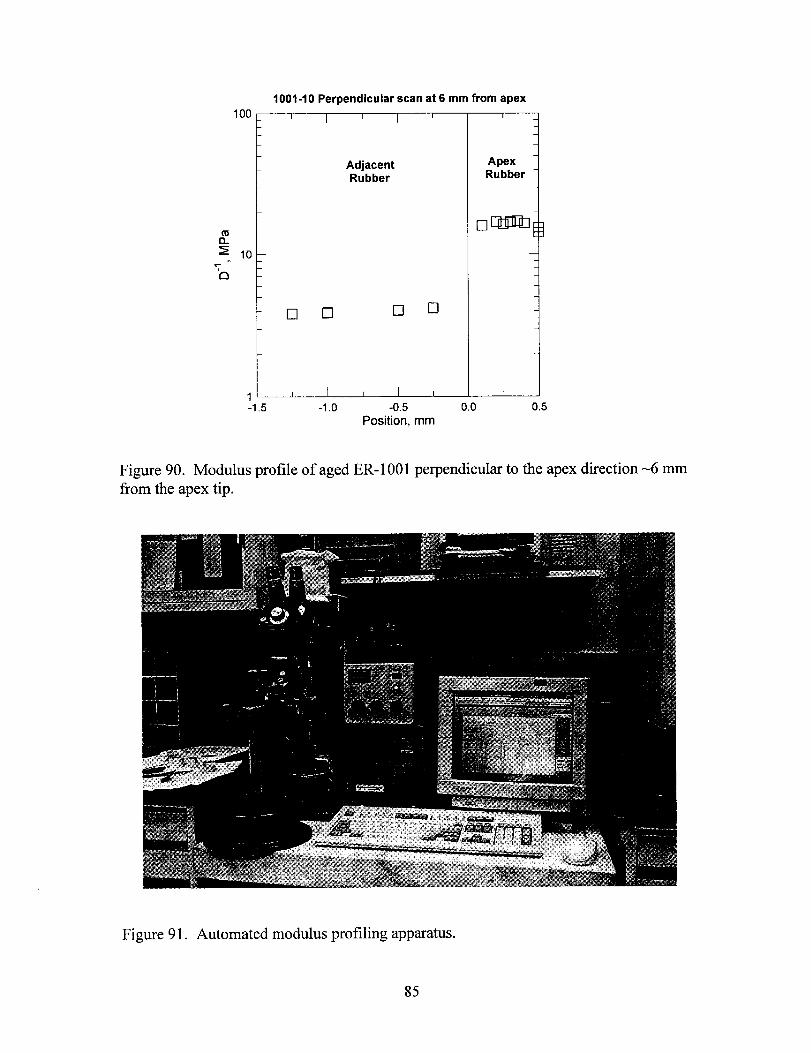
1001-10 Perpendicular scan at 6 mm from apex100 p 1 I I
I1 1
i
CT2 ,(J .
‘7n
l—-1.5
AdjacentRubber
ApexRubber
❑m
I
❑ 0 ❑ o
I I 1 I I 1
-1.0 -0.5 0.0 0.5Position, mm
Figure 90. Modulus profile of aged ER-1 001 perpendicular to the apex direction -6 mmfrom the apex tip.
Figure 91. Automated modulus profiling apparatus.
85

●
Fi
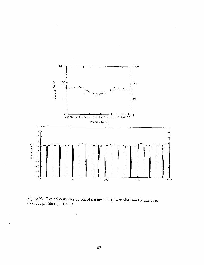
4
3
2 [
1000 I I I I 1 I I 1 I I I
i
1000
,~10.0 0.2 0.4 0,6 0.8 1.0 1.2 1.4 1.6 1.5 2.0 2.2
Position [mm]
z- 1~
0-6cm –1iii u—2 -
-3 -
–4
-50
l—
1500
5 I
n
11000 1500
r
—
J--
—
2000
Figure 93. Typical computer output of the raw data (lower plot) and the analyzedmodulus profile (upper plot).
87
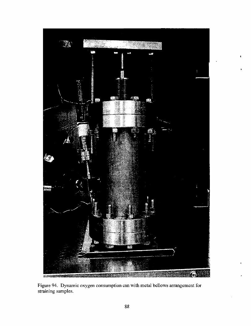
Figure 94. Dynamic oxygen consumption can with metal bellows arrangement forstraining samples.
88

Figure 95. Dynamic oxygen consumption setup.
89

Figure 96, Detail showing how samples are connected to the metal bellows.
90

u)~
E3 –yo
C-o.=
p –u)co0sa)El
6
00 200 400 600 800 1000
Aging time at 72°C
Figure 97. Inte~ated oxygen conswption results for Matefid l54uderstaticmddynamic aging conditions.
Figure 98. Interracial Force Microscope (IFM) currently under construction.
91
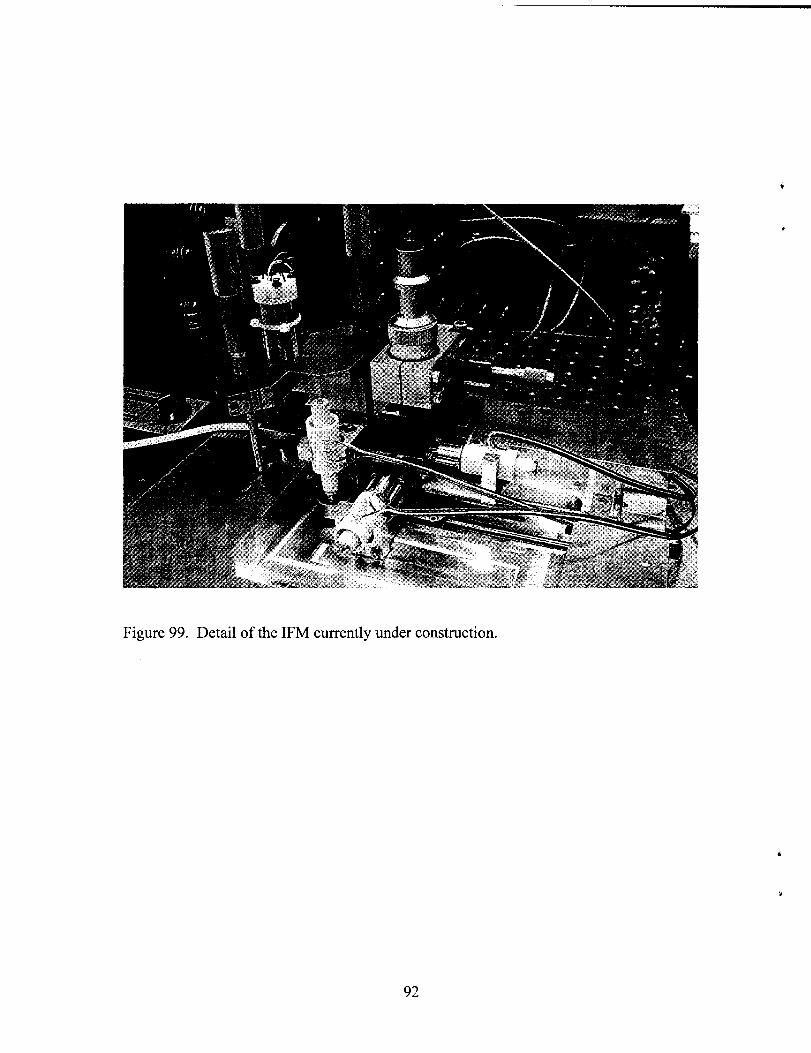
92

APPENDIX1
PROCEDURES FOR GC ANALYSIS OF GAS SAMPLES
FOR MEASUREMENT OF OXYGEN CONSUMPTION RATES
J. Wise
December7, 1995
1 Introduction
This document describes the procedures for our system of measuring oxygen consumption rates
using gas chromatography. There are two primary parts to this document. Section 2 describes how
to design and assemble a sample container; sections 3 to 6 give specific instructions for using the
gas chromatography to perform the analysis.
2 Sample Preparation
To prepare a sample for oxygen uptake measurements, it is necessary to consider what information is
desired from the measurement, so that appropriate trade-offs between sample mass and time interval
of the measurement can be made. For example, if the goal is to obtain a series of measurements
to determine how the consumption rate changes with time, it may be preferable to use smaller
sample masses and correspondingly longer time intervals. The advantage in this case is that fewer
measurements would be required, allowing the overall set of measurements can be completed in
less time (note that there can be significant amounts of idle time between oven aging segments).
Conversely, if the goal is to obtain only one or two measurements rather than a series, it may
be preferable to use more massive samples so that data can be obtained quickly. Obviously, it
is necessary to consider the available sample mass when designing a set of experiments. When
determining the time interval for which a sample is aged, I have adopted the standard of rounding
to the nearest 24 hr increment. Because of uncertainty in the time required for sample containers
to equilibrate at their aging temperature, I have set 72 hr as an arbitrary minimum aging time.
For series of consumption measurements, 7 day or 14 day intervals are often convenient.
1. To establish the specific lengths of time and sample masses for specific aging tests, we use
the relationw c1
Vf=(jt’(1)
93

which is derived from the ideal gas law; W is the sample mass [g], Vf is the free (gas) volume
of the container [cm3], Cl is a constant whose value is described below [mol/cm3], 4 is the
(anticipated) oxygen consumption rate [mol/g-s], and t is the aging time [s]. From the ideal
gas law, the constant C’I is given byAp
cl==, (2)
where Ap is the change in gas pressure (measured at the aging temperature) in the containerj
during aging, R is the gas constant, and T is the absolute temperature at which the aging
occurs. From eqn. 2 it is clear that Cl varies with temperature and also with the desired Ap.
Values of Cl such that the average pressure during aging will be N130 Torr (or N40 Torr, for
measurements of ~) for many common designs of aging tests are listed in Table 1.
Table 1: Design constants for backfilling containers.
Aging
T, ‘C
160
140
125
110
96
80
65
52
40
23
Ap = 60 Torr (160 + 100)
cl
2.23x10⁻⁶
2.33x10⁻⁶
2.42x10⁻⁶
2.51x10⁻⁶
2.61x10⁻⁶
2.73x10⁻⁶
2.85x10⁻⁶
2.95x10⁻⁶
3.07X10⁻⁶
3.26x10⁻⁶
Pbackfill~Torr
109.4
114.3
119.4
123.1
128.0
134.4
140.3
145.5
150.9
160.0
Ap= 40 Torr (150 + 110)
1.48x10⁻⁶
1.55X10⁻⁶
1.61x10⁻⁶
1.67x10⁻⁶
1.74X10⁻⁶
1.82x10⁻⁶
1.90X10⁻⁶
1.97X10⁻⁶
2.05x10⁻⁶
2.17x10⁻⁶
PbackfillITOrr
102.7
107.1
111.9
115.4
120.0
126.1
131.6
136.4
141.5
150.0
Ap = 20 Torr (50 + 30)
Pbackfill)Torrc1
7.43X10⁻⁷
7.79xlo-7
8.08X10⁻⁷
8.40x10⁻⁷
8.72x10⁻⁷
9.11X10⁻⁷
9.52x10⁻⁷
9.90X10⁻⁷
1.03X10⁻⁶
1.O9X1O–6
34.2
35.8
37.2
38.6
40.1
41.9
43.8
45.5
47.3
50.0
2. After the appropriate sample mass is determined, the sample must be cut so that it will fit
into the sample container. Additionally, the sample must be cut sufficiently thin to avoid
diffusion-limited oxidation (DLO) effects. We calculate L., the critical thickness to preclude
DLO effects as~ = 2pPox 0’5
c() 4’
(3)
where p is the average oxygen partial pressure surrounding the sample, POX is the oxygen●
‘ permeability coefficient, and ~ is the oxygen consumption rate.
Because setting up new containers or modifying the contents of existing containers is a time- 2
consuming process, it is prudent to initially cut the samples so that they will be suitable
94
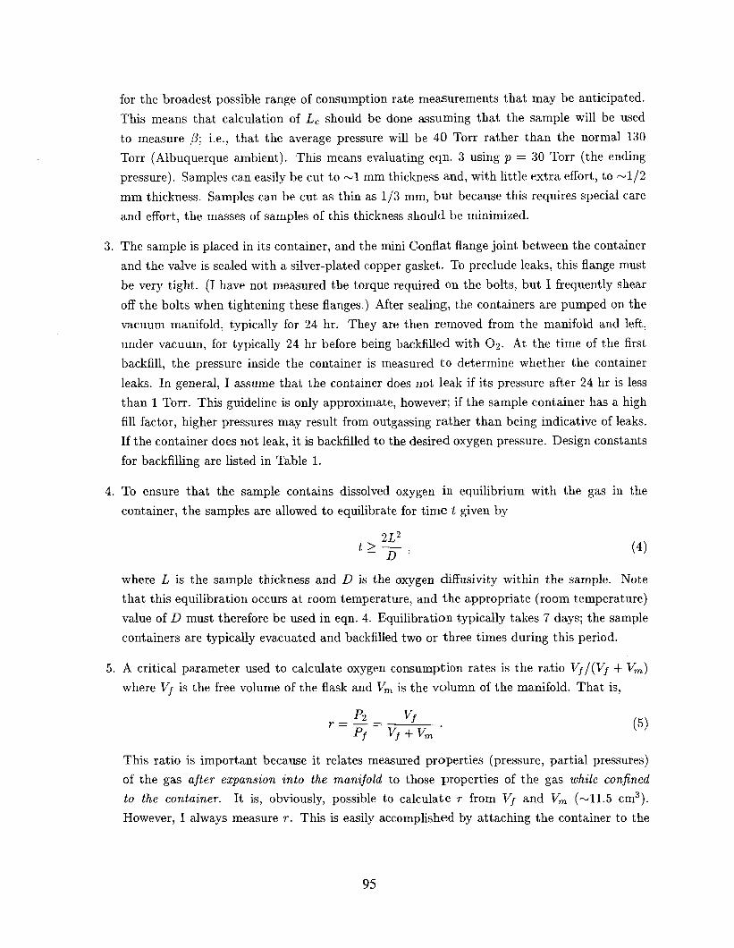
3.
4.
5.
for the broadest possible range of consumption rate measurements that may be anticipated.
This means that calculation of Lc should be done assuming that the sample will be used
to measure ~; i.e., that the average pressure will be 40 Torr rather than the normal 130
Torr (Albuquerque ambient). This means evaluating eqn. 3 using p = 30 Torr (the ending
pressure). Samples can easily be cut to N1 mm thickness and, with little extra effort, to N1/2
mm thickness. Samples can be cut as thin as 1/3 mm, but because this requires special care
and effort, the masses of samples of this thickness should be minimized.
The sample is placed in its container, and the mini Conflat flange joint between the container
and the valve is sealed with a silver-plated copper gasket. To preclude leaks, this flange must
be very tight. (I have not measured the torque required on the bolts, but I frequently shear
off the bolts when tightening these flanges. ) After sealing, the cent ainers are pumped on the
vacuum manifold, typically for 24 hr. They are then removed from the manifold and left,
under vacuum, for typically 24 hr before being backfilled with 02. At the time of the first
backfill, the pressure inside the container is measured to determine whether the container
leaks. In general, I assume that the container does not leak if its pressure after 24 hr is less
than 1 Torr. This guideline is only approximate, however; if the sample container has a high
fill factor, higher pressures may result from outgassing rather than being indicative of leaks.
If the container does not leak, it is backfilled to the desired oxygen pressure. Design constants
for backfilling are listed in Table 1.
To ensure that the sample contains dissolved oxygen in equilibrium with the gas in the
container, the samples are allowed to equilibrate for time t given by
2L2t>—
D’(4)
where L is the sample thickness and D is the oxygen diffusivity within the sample. Note
that this equilibration occurs at room temperature, and the appropriate (room temperature)
value of D must therefore be used in eqn. 4. Equilibration typically takes 7 days; the sample
containers are typically evacuated and backfilled two or three times during this period.
A critical parameter used to calculate oxygen consumption rates is the ratio Vf /(Vf +
where Vf is the free volume of the flask and V~ is the volumn of the manifold. That is,
P2 Vf
‘=q=vf+vm”
Vm)
(5)
This ratio is important because it relates measured properties (pressure, partial pressures)
of the gas after expansion into the manijoid to those properties of the gas while confined
to the container. It is, obviously, possible to calculate r from Vf and Vm (Nil.5 cm3).
However, I always measure r. This is easily accomplished by attaching the container to the
95
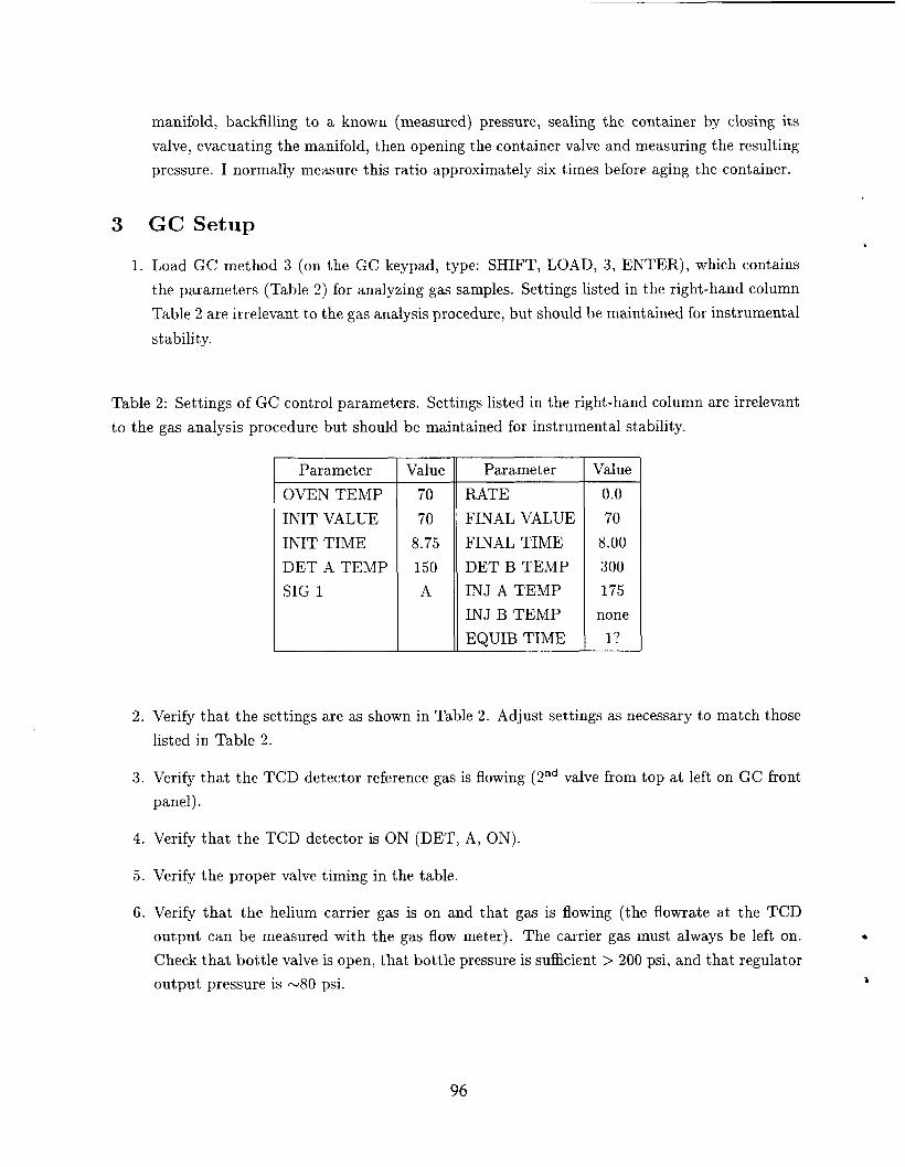
. . . . . . .. . . . . . . .
3
1
manifold, backfilling to a known (measured) pressure, sealing the cent airier by closing Its
valve, evacuating the manifold, then opening the container valve and measuring the resulting
pressure. I normally measure this ratio approximately six times before aging the container.
GC Setup&
Load GC method 3 (on the GC keypad, type: SHIFT, LOAD, 3, ENTER), which contains
the parameters (Table 2) for analyzing gas samples. Settings listed in the right-hand column
Table 2 are irrelevant to the gas analysis procedure, but should be maintained for instrumental
stability.
Table 2: Settings of GC control parameters. Settings listed in the right-hand column are irrelevant
to the gas analysis procedure but should be maintained for instrumental stability.
2.
3.
4.
5.
6.
Parameter
OVEN TEMP
INIT VALUE
INIT TIME
DET A TEMP
SIG 1
Value
70
70
8.75
150
A
Parameter Value
RATE 0.0
FINAL VALUE 70
FINAL TIME 8.00
DET B TEMP 300
INJ A TEMP 175
INJ B TEMP none
EQUIB TIME { 1?
Verify that the settings are as shown in Table 2. Adjust settings as necessary to match those
listed in Table 2.
Verify that the TCD detector reference gas is flowing (2nd valve from top at left on GC front
panel).
Verify that the TCD detector is ON (DET, A, ON).
Verify the proper valve timing in the table.
Verify that the helium carrier gas is on and that gas is flowing (the flowrate at the TCD
output can be measured with the gas flow meter). The carrier gas must always be left on. ●
Check that bottle valve is open, that bottle pressure is sufficient >200 psi, and that regulator
output pressure is w80 psi. a
96

7. Verify that the control gas to actuate the valves in on. (This gas is normally on. ) Check that
bottle valve is open and regulator output pressure is N65 psi.
8. (Optional: only necessary if planning to backfill containers with oxygen. ) Turn on oxygen
backfill gas. Open bottle valve and verify that regulator output pressure is N1O psi.)
9. (Optional: only necessary if planning to obtain GC calibration curve.) Turn on calibration
gas. Open bottle valve and verify that regulator output pressure is w14 psi.)
10. Delete any existing integrator time program (On the integrator keypad, type: DEL, TIME,
ENTER). Verify that the time program has been deleted by printing the current time program
(LIST, TIME, ENTER).
11. Desirable, although optional, settings for the integrator are: attenuation = 2° (ATT 2t, O,
ENTER), threshold = O (THRSH, O, ENTER), and chart speed = 1 (CHT SP, 1, ENTER).
The parameters attenuation and threshold affect only the appearance of the printed output;
they do not affect the integration calculations. Chart speed is set to its minimum value to
conserve paper. To print all current integrator parameters, type LIST, LIST on the integrator
keypad.
12. Turn on the vacuum pump. The switch is on the pump, which is on the floor under the bench.
13. Turn on the pressure gauge. The switch is on the digital pressure meter, which is on the
bench, in the monkey bars.
14. Open valves VB and Vc, to evacuate the manifold.
15. Open the calibration gas valve (VD)to purge the calibration gas supply line. Close the cali-
bration gas valve VD.
16. Open the oxygen valve (VE) to purge the oxygen supply line. Close the oxygen valve VE.
4 Calibration.
The GC must be calibrated using the external standard gas mixture. The composition of this
gas is is given in Table 3. As a practical matter, it is best to begin the calibration procedure
with one or two analyses of pure 02 at pressures of N1OO Torr; this seems to help stabilize the
detector. Typically 10–15 calibration points with the standard gas are required for the detector
to stabilize. I recommend beginning the calibration at w1200 Torr of calibration gas and taking
points at intervals of w200 Torr as the pressure is reduced and then at intervals of N200 Torr as the
pressure is increased. That is, taking points at 1200, 1000, 800...200, 100, 300...900, 1100. The
first four or five points will typically fall below the calibration that is established by the remaining
97
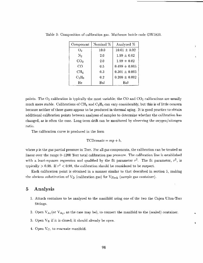
Table 3: Composition of calibration gas. Matheson bottle code GW5831.
Component
02
N2
C02
co
CH4
CZHG
He
Nominal $ZO
10.0
2.0
2.0
0.5
0.3
0.2
Bal
Analyzed %
10.01 + 0.02
1.99 + 0.02
1.99 * 0.02
0.499 + 0.005
0.301 + 0.003
0.200 ● 0.002
Bal
points. The 02 calibration is typically the most variable; the CO and C02 calibrations are usually
much more stable. Calibrations of CH4 and CZHG can vary considerably, but this is of little concern
because neither of these gases appear to be produced in thermal aging. It is good practice to obtain
additional calibration points between analyses of samples to determine whether the calibration has
changed, as is often the case. Long-term drift can be monitored by observing the
ratio.
The calibration curve is produced in the form
TCDcounts = mp + b,
oxygen/nit rogen
where p is the gas partial pressure in Torr. For all gas components, the calibration can be treated as
linear over the range 0-1200 Torr total calibration gas pressure. The calibration line is established
with a least-squares regression and qualified by the fit parameter r2. The fit parameter, r2, is
typically >0.98. If r2 <0.98, the calibration should be considered to be suspect.
Each calibration point is obtained in a manner similar to that described in section 5, making
the obvious substitution of VD (calibration gas) for VFl=k (sample gas container).
5
1.
2.
3.
4.
Analysis
Attach container to be analyzed to the manifold using one of the two the Cajon Ultra-Torr
fittings.
Open VA, (or V&, as the case may be), to connect the manifold to the (sealed) container.
Open VB if it is closed; it should already be open.
Open Vc, to evacuate manifold.
98
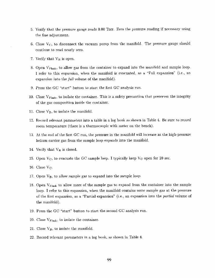
5. Verify that the pressure gauge reads 0.00 Torr. Zero the pressure reading if necessary using
the fine adjustment.
6. Close Vc, to disconnect the vacuum pump from the manifold. The pressure gauge should
continue to read nearly zero.
7. Verify that VB is open.
8. Open VFlask, to allow gas from the container to expand into the manifold and sample loop.
I refer to this expansion, when the manifold is evacuated, as a “Full expansion” (i.e., an
expansion into the ~ull volume of the manifold).
9. Press the GC “start” button to start the first GC analysis run
10. Close VFl=k, to isolate the container. This is a safety precaution that preserves the integrity
of the gas composition inside the container.
11. Close VB, to isolate the manifold.
12. Record relevant parameters into a table in a log book as shown in Table 4. Be sure to record
room temperature (there is a thermocouple with meter on the bench).
13. At the end of the first GC run, the pressure in the manifold will increase as the high-pressure
helium carrier gas from the sample loop expands into the manifold.
14. Verify that VB is closed.
15. Open Vc, to evacuate the GC sample loop. I typically keep VC open for 20 sec.
16. Close Vc.
17. Open VB, to allow sample gas to expand into the sample loop.
18. open VFIMk to allow more of the sample gas to expand from the container into the sample
loop. I refer to this expansion, when the manifold contains some sample gas at the pressure
of the first expansion, as a “Partial expansion” (i.e., an expansion into the pa~tial volume of
the manifold).
19. Press the GC “start” button to start the second GC analysis run.
20. (hse vFl=k, h isolate the container.
21. Close VB, to isolate the manifold.
22. Record relevant parameters in a log book, as shown in Table 4.
99
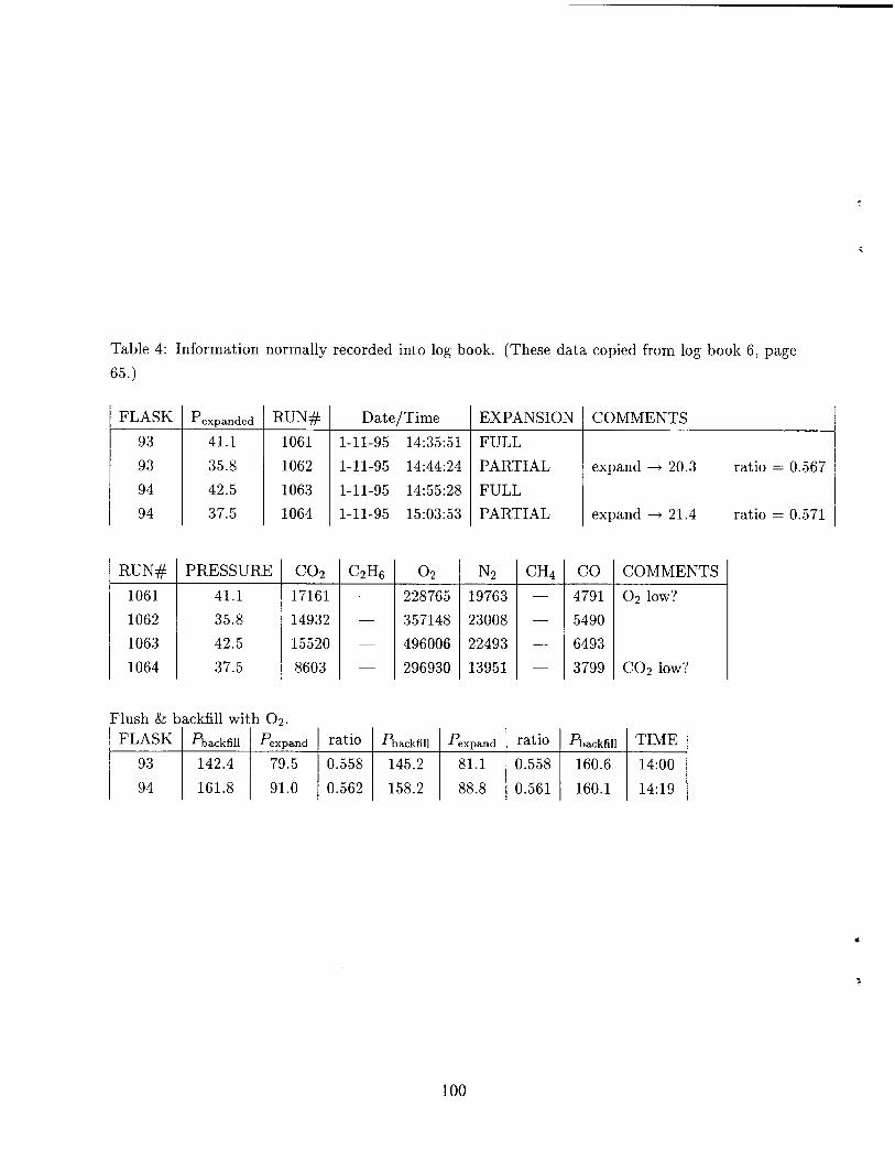
Table 4: Information normally recorded into log book. (These data copied from log book 6, page
65.)
FLASK Pexpan&~ RUN#
93 41.1 1061
93 35.8 1062
94 42.5 1063
94 37.5 1064
TRUN# PRESSURE
1061 41.1
1062 35.8
1063 42.5
1064 37.5
C02
Date/Time
1-11-95
1-11-95
1-11-95
1-11-95
I CZHG
17161 —
14932 —
15520 —
8603 —
Flush & backfill with 02.
ratio
0.558
0.562
14:35:51
14:44:24
14:55:28
15:03:53
02
228765
357148
496006
296930
Pbackfi]l
145.2
158.2
EXPANSION I COMMENTS
FULL
PARTIAL
FULL
PARTIAL
—N2
19763
23008
22493
13951
P expand
81.1
88.8
CH4—
—
—
rat io
0.558
0.561
expand + 20.3
expand + 21.4
co
4791
5490
6493
3799
COMMENTS
l’backfill
160.6
160.1
02 low?
C02 low?
TIME
14:00
14:19
ratio = 0.567
ratio = 0.571
100

23. After both analyses, the container is evacuated and backfilled with 02 as shown in Table 4.
24. The container is then left to equilibrate before being aged again.
I have chosen to do two analyses of each container, as described above. I believe this is prudent
because of the occasional bad separation. My standard analysis procedure is to use one full and one
partial expansion; this was derived from an attempt to conserve sample gas between runs when the
sample was particularly valuable (i.e., the container volume was small or the container had been
aged for an especially long time). When, as happens occasionally due to operator error, the sample
gas stored in the manifold is contaminated or lost, it is possible to perform the analysis as two full
expansions.
6 GC Shutdown
1. Load GC method 1 (SHIFT, LOAD, 1, ENTER), to put the GC into its standby mode.
2. Verify that valves VD (calibration gas) and VE (oxygen) are closed, to isolate the manifold
from the calibration gas and oxygen supplies.
3. Verify that valves VA, and VA, (at Cajons Ultratorr ports) are closed.
4. Verify that VB is open.
5. Remove all sample containers from the manifold.
6. Open Vc, to evacuate the manifold.
7. Close Vc.
8. Turn off the vacuum pump.
9. Open the bleeder valve, to bleed the line between the manifold and the vacuum pump.
10. Close the bleeder valve.
11. Turn off the pressure gauge.
12. Close the valve on the calibration gas bottle.
13. Close the valve on the oxygen bottle.
101

7 Miscellany
1. When reading pressures on the digital pressure meter, the observed reading must be multiplied
by 10 to give the pressure in Torr. This is true regardless of whether the pressure meter is
set to the high or low range.
2. When I refer to a valve as being “open,” the only critical valves are VAZ, VB, and VFlak. I
define the first two of these valves as open when the handle has been turned just to the point
when the internal spring no longer exerts pressure on the handle. I define VFla.k as open
when cracked open plus approximate ely 1/4 turn.
102
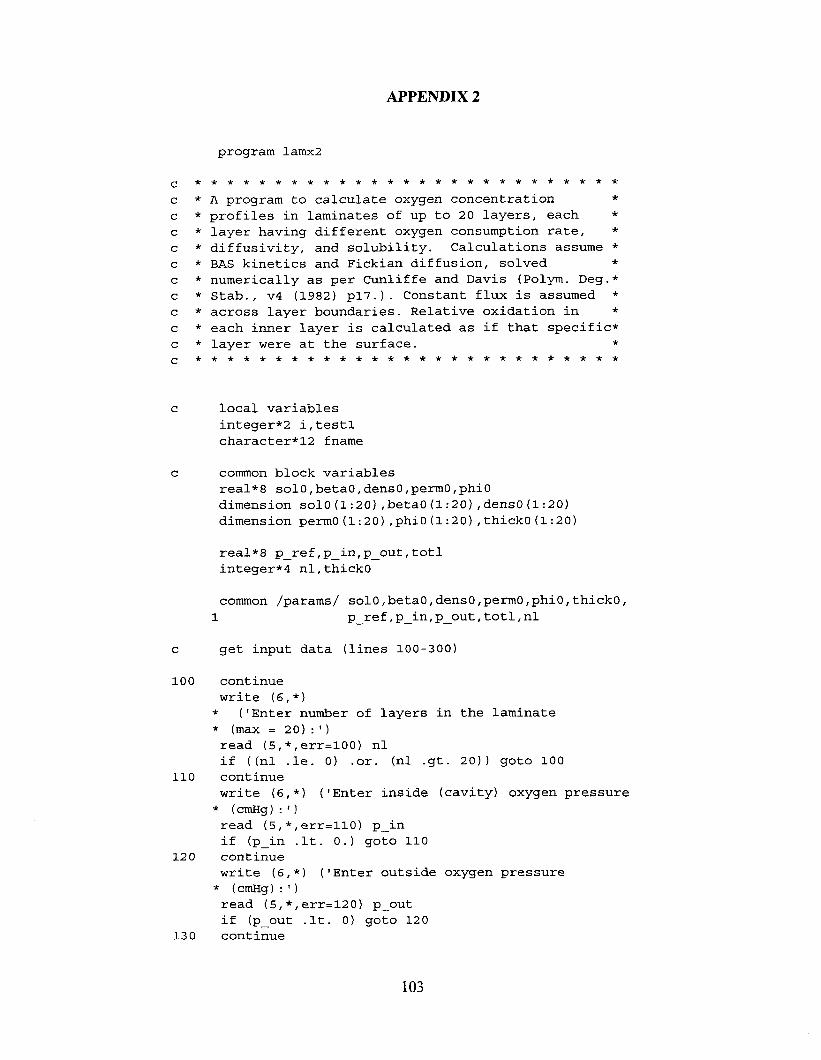
program lamx2
c ******** ******** ******** ***
c * A program to calculate oxygen concentration *
c * profiles in laminates of up to 20 layers, each *c * layer having different oxygen consumption rate, *
c * diffusivity, and volubility. Calculations assume *c * BAS kinetics and Fickian diffusion, solved *
c * numerically as per Cunliffe and Davis (Polym. Deg.*
c * Stab., V4 (1982) p17.) . Constant flux is assumed *
c * across layer boundaries. Relative oxidation in *
c * each inner layer is calculated as if that specific*
c * layer were at the surface. *
c ******** ******** ******** ***
c local variables
integer*2 i,testl
character*12 fname
c common block variables
real*8 solO,betaO,densO,permO,phiO
dimension so10(l:20),beta0 (l:20),dens0 (1:20)
dimension permO(l :20),phi0 (l:20),thick0 (1:20)
real*8 p_ref,p_in,p_out, totl
integer*4 nl,thickO
common /params/-11
c get input data
100 continuewrite (6,*)
solO,betaO, densO,permO ,phiO,thickO,
p_ref,??_in,p_out ,totl,nl
lines 100-300)
* (’Enter nutier of layers in the laminate* (max= 20):’)
read (5,*,err=100) nl
if ((nl le. O) or. (nl .gt. 20)) goto 100
110 continue
write (6,*) (‘Enter inside (cavity) oxygen pressure
* (Cmg):’)
read (5,*,err=l10) p_in
if (p_in .lt. O.) goto 110
120 continuewrite (6,*) (’Enter outside oxygen pressure
* (Cmg):’)
read (5,*,err=120) p out—if (p out .lt. O) goto 120—
130 continue

c
140
150
11
21
31
41
5161
211
221
231
241
251
261
300
c
400
for our data in Albuquerque, use p_ref . 13.2
write (6,*) (‘Enter reference oxygen pressure
* (cmHg) :’)
read (5,*) p ref
if (p ref .1;. o) goto 130.continue
write (6,*) (‘Enter total laminate thickness
* (cm):’)
read (5,*,err=140) totl
if (totl le. O) goto 140
continue
write (6,*)
* (’Enter filename in which to save calculated
* profile:’)
read (5,’ (a12) ‘,err=lsO) fnameformat (’Enter thickness [total = 1000] of layer
*I ,i2,’ :’)
format (’ Enter 02 consumption rate (mol/g-s) of
* layer ‘,i2, !:J)
format (’ Enter 02 permeability (ccSTP/cm-s-cmHg)
* of layer ‘,i2,’ :1)
format (’ Enter volubility (ccSTP/cm3-cmHg) of
* layer ‘,i2,’ :’)
format (’ Enter density (g/cm3) of layer ‘,i2, ‘:’)
format (’ Enter beta of layer ‘,i2, ‘:’)
testl = O
do 300, i = l,nl
write(6,11) i
read(5,*,err=211) thickO(i)
write(6,21) i
read(5,*,err=221) phiO(i)
write(6,31) i
read(5,*,err=231) permO (i)
write(6,41) i
read(5,*Jerr=241) solO(i)
write(6,51) i
read(5,*,err=251) densO(i)
write(6,61) i
read(5,*,err=261) betaO (i)
testl = testl + thickO(i)
continue
test that fractional thickness sum to unity
continue
IF (testl .ne. 1000.) THEN
testl = O
write (6,*)* (’Layer thicknesses did not sum to 1000’)
do 45o, i = l,nl
write(6Jll) i
read(5,*) thickO(i)
104

testl = testl + thickO(i)
450 continue
if (testl .ne. 1000.) goto 400
ENDIF
c
c
c
c
c
c
c
c
c
c
c
c
call subroutine to calculate oxidation profiles
call calcl(fname)
return
end
***-k*********** *************** *************** *
subroutine calcl (fname)
constant flux across layer boundaries; assume no
reaction in intervals i+l and i-1 adjacent to
boundary--this introduces only insignificant error.
Flux calculation with volubility change across
layers :
D(i+l) * ( theta(j-1) - S(i+l)/S(i)*theta(j) )
= D(i) * ( theta(j) - theta(j-1) )
integer*4 i,j, k,n,start,stop
real*8 iter2,p2, th0,c_in, c_out
real*8 theta,relcharacter*12 fname
dimension theta (0:1000), rel(O:lOOO)
real*8 solO,betaO, densO,permO,phiO
real*8 p ref,p_in,p_out, totl ,maxtheta—real*8 phi i,alpha i,beta_i
integer*4 ~l,thick~
dimension so10(l:20),beta0 (l:20),dens0 (1:20)
dimension permO(l :20),phiO(l:20), thickO(l:20)
common /params/ solO,betaO, densO,permO,phiO, thickO,* p_reffp_inrp_out ~totlznl
number of intervals
k = 1000.
c_in = p_in*so10 (l)
c_out = p_out*solO(nl)
boundary conditions
theta(k) = 1.
thO = c_in/c_out
prepare initial iteration: guess theta(k-1)
105

c
c
600
c
610
620
700
c
c
c
maxtheta = max(thO,theta(k))theta(k-1) = maxthetap2 = 1.
iter2 = maxtheta
calculate theta(k-2) ... theta(0)
i refers to a specific layer within the composite
write(6,*) ‘Working. ..‘
continue
start = k-1
stop = k-thickO(nl)+l
do 620, i = nl,l,-1
correct beta, phi for p_out .ne. p_ref
beta_i = betao(i)*p_out/p_ref
phi i = phiO(i)*(l+betaO(i))/( (p_ref/p_out) +—* betaO(i))
alpha_i =
* (22400*phi i*totl*totl*densO(i))/(p_out*permO (i))
alpha_i =–alpha i*(beta_i+l)—
do 610, j = start,stop,-1
theta(j-1) =* (alpha_i*theta (j)/(((beta_i*theta (j))+l)*k*k))* + (2*theta(j)) - theta(j+l)
if (j .eq. 1) goto 700IF (theta(j-l) .lt. O) THEN
theta(j) < 0 is physically meaningless.
To prevent math errors, terminate this
iteration and proceed to next iteration.
we set theta(0) = theta(j-1) < 0 to indicate
that the current trial value of theta(k-1) is
too small.
theta(0) = theta(j-1)
goto 710
ENDIF
continue
rel (stop-1) = rel(stop)
if (i .eq. 1) goto 620
j = stop - 1
theta(j-1) = (solO(i-1)/solO(i))*theta (j)* + (permO(i) *so10 (i-1))/(permO(i-l)*so10 (i))** (theta (j)-theta(j+l) )
theta(j) = theta(j)*solO(i-1)/so10 (i)
start = start - thickO(i)
stop = stop - thickO(i-1)
continue
continue
test whether iteration is within specified
agreement
if (dabs(theta(O) - thO) .lt. 0.005) goto 800
prepare for next iteration
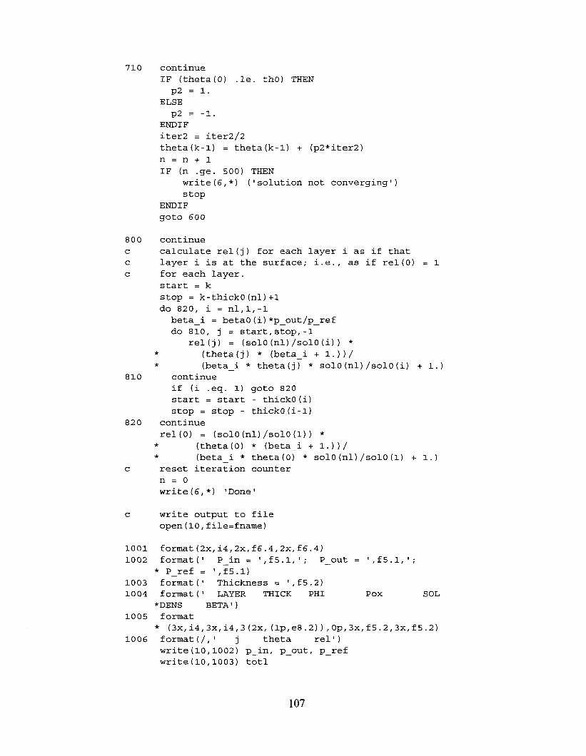
710 continue
IF (theta(0) le. thO) THEN
p2 = 1.
ELSE
p2 = -1.
ENDIF
iter2 . iter2/2
theta(k-1) = theta(k-1) + (p2*iter2)
n.n+l
IF (n .ge. 500) THEN
write(6,*) (’solution not converging’)
stop
ENDIF
goto 600
800 continue
c calculate rel(j) for each layer i as if that
c layer i is at the surface; i.e., as if rel(0) = I
c for each layer.
start . k
stop = k-thickO(nl)+l
do 820, i = nl,l,-1
beta_i = betaO(i)*p_out/p_ref
do 810, j = start,stop,-1rel(j) = (solO(nl)/solO(i)) *
* (theta(j) * (beta_i + 1.))/* (beta_i * theta(j) * solO(nl)/solO(i) + 1.)
810 continue
if (i .eq. 1) goto 820
start = start - thickO(i)
stop = stop - thickO(i-1)
820 continue
rel(0) = (solO(nl)/solO(l)) ** (theta(0) * (beta_i + 1.))/* (beta_i * theta(0) * solO(nl)/solO(l) + 1.)
c reset iteration countern=o
write(6, *) ‘Done’
c write output to file
open(lO, file=fname)
1001 format (2x,i4,2x,f6.4,2x, f6.4)
1002 format(’ Pin= ‘,f5.1,’; P out = ‘,f5.1,’;—* P ref = ‘,:5.1)
1003 fo;mat(’ Thickness = ‘,f5.2)
1004 format(’ LAYER THICK PHI Pox SOL
*DENS BETA ‘)
1005 format
* (3x,i4,3x, i4,3(2x, (lp,e8.2) ),0p,3x, f5.2,3x,f5.2)
1006 format(/, ‘ j theta rel r )write(10,1002) p in, p out, p_ref
write(10,1003) t~tl –
107

write (10,1004)
do 1100, i = l,nl
write (10,1005) i,thickO (i), phi O(i) , permO(i)J* sol O(i) , dens O(i), betaO (i)
1100 continue
write (10,1006)
do 1200, i = O,k,10
write(lO,1001) i/10, theta(i) , rel(i)
1200 continue
close(lO)
return
end
108

APPENDIX 3
MODULUS PROFILER- NOTES AND BLOCK DIAGRAMS
Tun on the computer and associated eWiPme~t. At the Dos P~OmP~type WIN and press Enter. Windows Program Manager appears. use tneleft mouse button to click on the “LABTECH NOTEBOOK PRO” icon; theLABTECH icons appear, Click on the LABTECH Build-Time icon; theBuild-Time screen opens. Click on File in the menu bar: click onOpen(be careful to not click on any other items in this screen) .
Double click on “C:\” folder in the I!irectories box. Press the
down arrow(keyboard) until NBP WIN appears and double click on it.In the File name box double ciick on “30.5ECNE1.LTC”. This is theLabtecn proqram th~t runs the Surface Modulus Profiler. Icons will
aPP@ar in the Build-Time window. The program is now ready to run.Ensure that the linear actuator screw that raises and lowers theprobe and weight is located at it’s maximum height. (This onlyneeds to be done for the initial installation) . Do this byunscrewing it from the aluminum block-that holds the weight hook.Continue unscrewing it(ccw) until it is as high as it will go.Raise the aluminum weiqht block threads to the screw. Continuetuzning the screw cc-~ while holding the weight block threads tothe threads on the erd of the screw until a click or deten~ isfelt. This happens wnea the leading edge of the threads are readyto engage. At this point turn the screw cw and screw it into thewei5nt block. This 2s the stzrting position for a test run.The probe can be re.ised and lowe:ed manually by selec~ing UP orDOWN with the UP-AUTO-DOWN switch and then p’usi?ingthe JOG switchmamentarilly. This is convenient when mounting a new sample oz toreposition the probe if the test is prematurely terminated. Toestablish the vertical location of the sa~le make sure there isno sample mounted. Se= the s-witch to DOWN cr UP as needed andwhile pushing down qe~tly on the probe weight tray push the JOGswitch momentarily ustil the DVM reads ES close to ie:o ESpossible. This is the “balanced” position thzt will proviae e30uG5p.rsbe travel while re.mainin~ in the lineaz zange of the L~T.Carefully(s~le sux~ace must be below the probe tip)mount zsample. Use tne microscope and DVM to adjcs: the Z-axis zr~czcmezezuztil the sample s“uxface just touches the FZOD@ tip. JOG the prG~~UP until it just c~ea:s the sample surface(app:ox. 10 mv on theDVM) . Sxitch back to AUTO.=nsu~e that the steppex(x axis)has enough travel to accomocate thethickness (span)of the sample. The sceppez c=n be rotated r,azually.Ki:h the zid cf the rriczoscope pcsitiori the s.erple just akove tksfirs: data point cz the riqht site of the s=pie. (The steppezmotcr moves the sample to the right; the last cata point will be
on the left side.) Use the X and Y micrometers on the XYZ sczge tsposition the sample. Record the X axis micrometer reading. Ratatethe stepper to the cppcsite side of the sample(the last datapoint)and record the r=ading. Subtract to get Che total S?SX ofthe sample. Return the steppe= to the beqinzing position.
Usinq the left mmse button click on the RUN icon ox L33TECE5,JILD-TI~ s=~=en. The data dis?12y will appear(LABTSCH VISION);L-sit until the display is complete -it will take a few seconcs.Click and c:ag the S?AN slider un~il the digital dis?lay i~dicatssthe sgan tk.at was m.essured then release the buz:on. Click azd dr~~cne POIh’TS slider tintil the display indicates the number cf points
zo be pzobed then release the button. Make ceztain that the
F!OTORS switch is cn then click and hold on the red OFF butronuntil it terns to czen ON button. The probe motor will run andthe probe will beFi~ to move down. A solenoid will be pulseti to?roviae vib:ation to assist the ciescent of the probe. A<race (representing iis-alaceme.nt of the probe in mils)will appearon the dz:z displzy. Tne probe motor will run for 5 seconcs thez
109
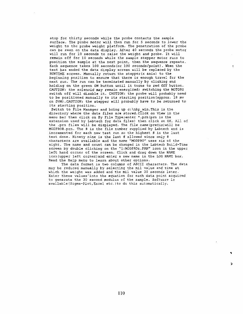
stop for thirty seconds while the probe contacts the samplesurface. The probe motor will then run for 5 seconds to lower theweight to the probe weight platform. The penetration of the probecan be seen on the data display. After 40 seconds the probe motorwill run for 10 seconds to raise the weight and probe. It willremain off for 10 seconds while the sample stepper motor runs toposition the sample at the next point, then the sequence repeats.Each sequence takes 100 seconds(or 100 seconds/point). When thetest has ended the data display screen will be replaced by theRUNTIME screen. Manually return the stepper(x axis) to thebeginning position to ensure that there is enough travel for thenext run. The run can be terminated manually by clicking and
holding on the green ON button until it turns to red OFF button.CAUTION: the solenoid may remain energized; switching the MOTORSswitch off will disable it. CAUTION: the probe will probably needto be positioned manually to its starting position(approx. 18 mvon DVM) .CAUTION: the stepper will probably have to be returned toits sta~ting position.Switch to File Manager and bring up c:\nbp win.This is the
directory where the data files are storeci.CTick on View in themenu bar then click on By File Type;enter *.prn(prn is theextension used by Labtech for data files) then click on OK, All ofthe .prn files will be displayed. The file name(prefix)will beMODPRO#.prn. The # is the file number supplied by Labtech and isincremented for each new test run so the highest # is the lasttest done. Ninety nine is the last # allowed since only 6characters are available and the name “MODPRO” uses six of theeight. The name and count can be changed in che Labtech Build-Timescreen by double clicking on the “l:MODPRO&.PRN” icon in the upperleft hand corner of the screen. Click and drag down the NAMEicon(upper left corner)and enter a new name in the LOG NAME box.Read the Help menu to learn about other options.
The data format is two columns of ASCII characters. The datamay be reduced manually by selecting the nril value and time atwhich the weight was added and the mil value 30 seconds later.Enter these values-into the equation for each data poi~t acquiredto generate the 30 second modulus of the sample. Software isavailable (Sigma-Plotr Excel etc.)to do this aurornatically.
110
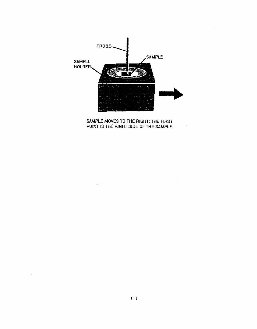
PROBE
41 SAMPLE
SAMPLEHOLDER
SAMPLE MOVES TO THE RIGHT; THE FIRSTPOINT IS THE RIGHT SIDE OF THE SAMPLE.
.
111
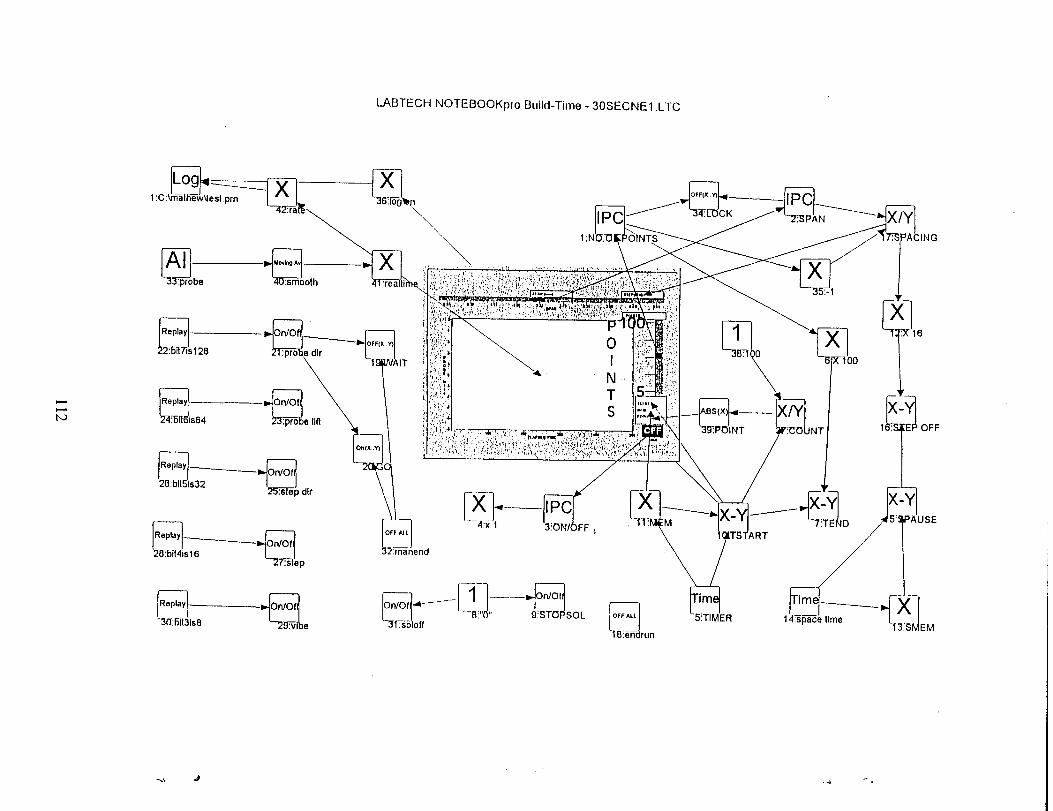
\\I
...
.:...4
1-
112
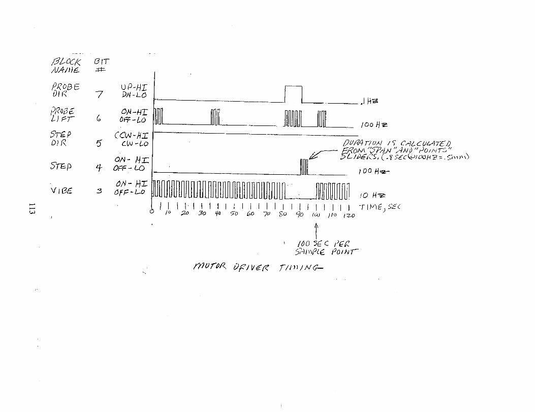
N
——
.
———&
-——
0U
3
——F
.,
E5 ——
0u
—–-R-11-
———s
-’R—
“
113
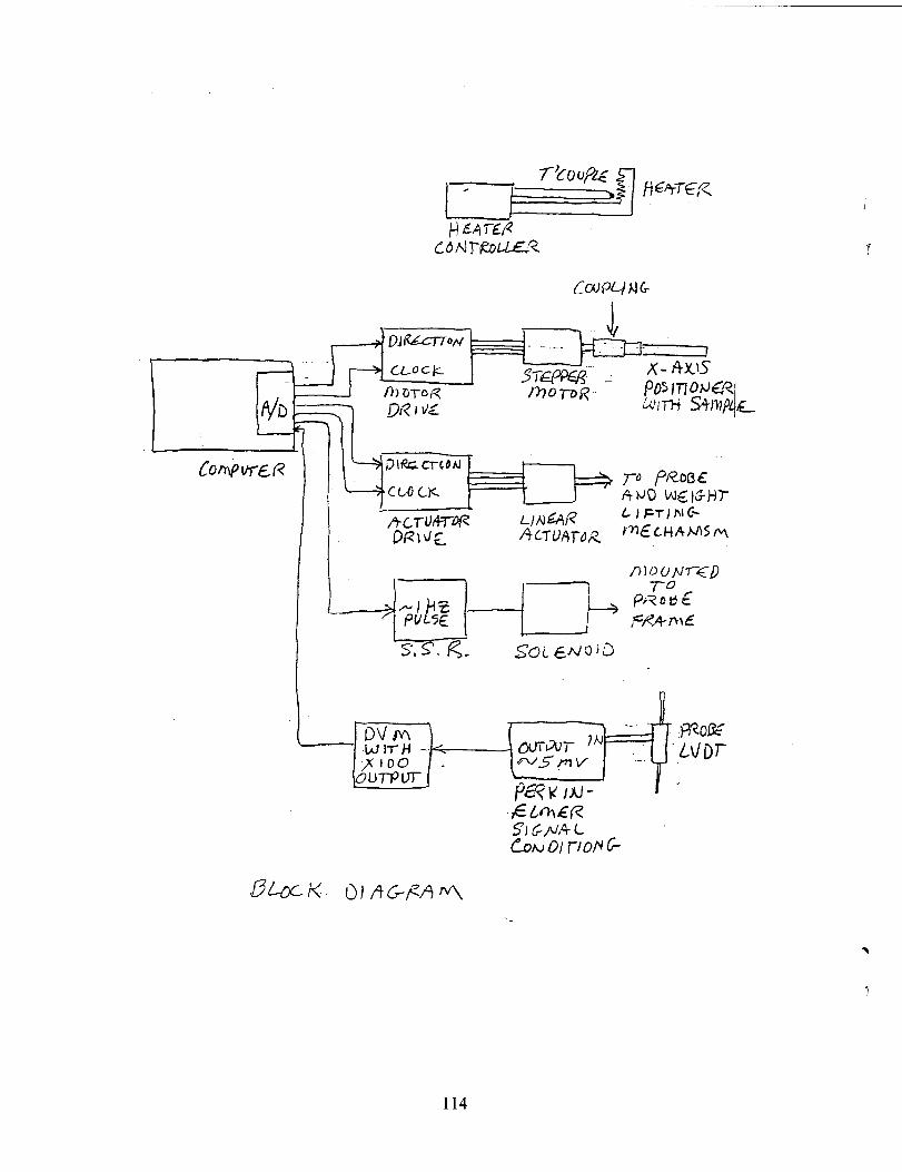
Cmfwa?
fw’r--~,<
-n “~-{Dv d-n...
w n- )-J -- @ilaJi- ‘N/xl f)cl - a/~)’rlv -IJ7-PVT j%qvJJU-
6UWRs) GN/4LCoNojIVOIN G
114
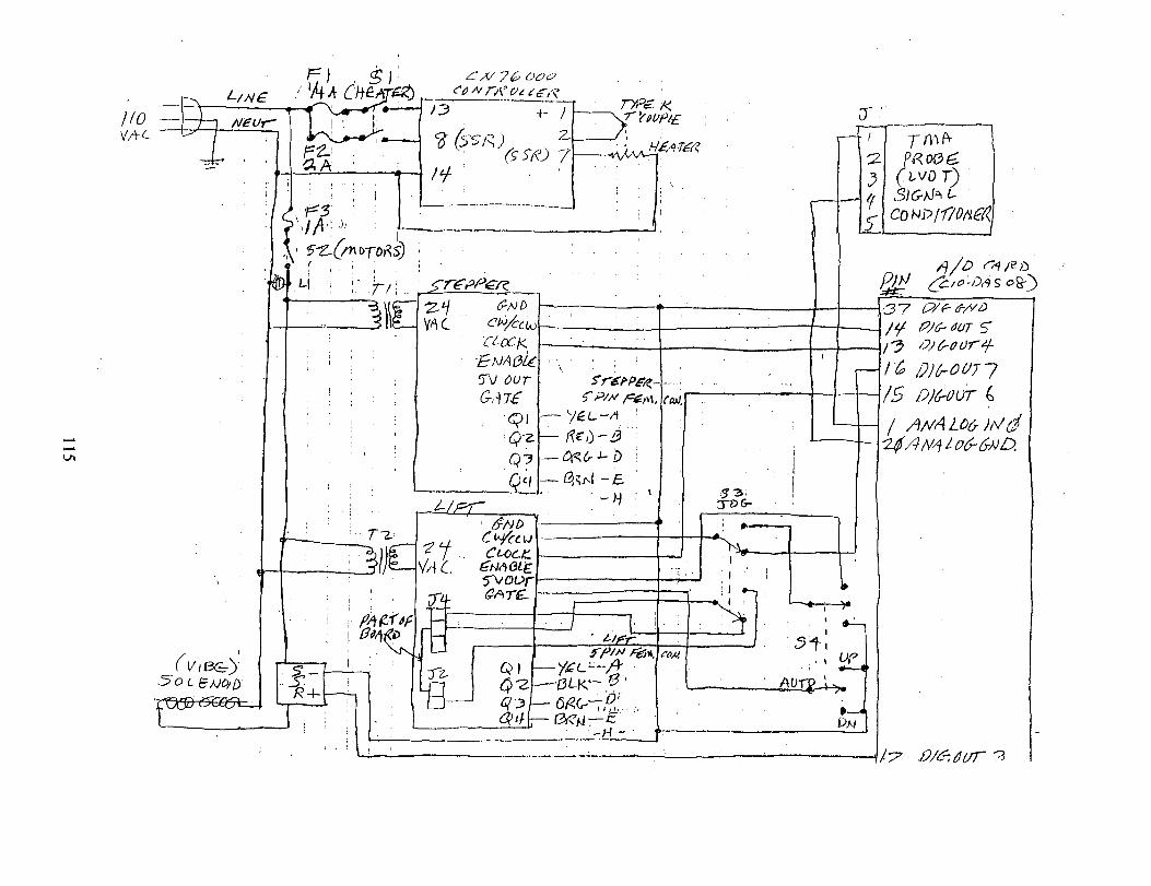
I
..W
$..”
x~....uj
.-—-
E-:1
L_ =l=J
TI--F
--A#?3?I
i&!.!
1Ill
1
--—-.,-6.
~,,,..2s7-—
‘-
..
ljsKG
&g\:
“-‘‘-”“-
‘“””““”
“-
““”“-
““---,“.
k-.
~\
“““--
;$
‘“\“
,.-
(1,
I+vw
if-)

Distribution
Former distribution in 1999 for SAND99-0465 under CRADA protection
1 MS1207 J. Wise , 5909 1 MS1407 P. Collins, 1811 1 MS1407 R.L. Clough, 1811 5 MS1407 K.T. Gillen, 1811 1 MS1435 A.K. Hays, 1800 3 MS9018 Central Technical Files, 8940-2 2 MS0899 Technical Library, 4916 2 MS0619 Review & Approval Desk, 15102 For DOE/OSTI 1 MS1380 Technology Transfer, 4212 Goodyear Distribution: 1 Al Causa 1 Dave Benko 1 Ed Terrill 1 John Lawrence 1 Dave Hargis 1 Library The Goodyear Tire and Rubber Company 142 Goodyear Boulevard Akron, OH 44305 Attention: Al Causa New distribution in 2012 for SAND2012-7644 1 MS1411 Celina Mathias C. 1819 1 MS1411 Gillen, Kenneth T. 1819 1 MS0899 Technical Library 9536 (electronic copy)
116